AFNI HOW-TO #3:
CREATING OPTIMAL STIMULUS TIMING FILES FOR
AN EVENT-RELATED FMRI EXPERIMENT
Table of Contents:
* Introduction: A hypothetical event-related FMRI study.
* Generate randomized stimulus timing files using AFNI 'RSFgen'.
* Create an ideal reference function for each stimulus timing file
using AFNI 'waver'.
* Evaluate the quality of the experimental design using AFNI
'3dDeconvolve'.
Before reading about the script provided in this HowTo, it may be helpful
to first visit the 'Background - the experiment' section and read up
on the various types of experimental designs used in FMRI research.
HowTo #3 differs from the previous HowTo's in that no sample data will be
introduced. Instead, the main focus will be to provide the reader with
information on how to generate the "best" randomized stimulus timing
sequence for an event-related FMRI study. With the aid of a script called
'@stim_analyze', we will generate many random timing sequences, and the
quality of each randomization order for the time series will be evaluated
quantitatively using AFNI '3dDeconvolve'. The results from 3dDeconvolve
will help us determine which stimulus timing sequence is most optimal for
our hypothetical FMRI study.
--------------------------------------------------------------------------------------------
--------------------------------------------------------------------------------------------
INTRODUCTION - A hypothetical event-related FMRI study
Suppose we are interested in examining how the presentation of 1) pictures,
2) words, and 3) geometric figures, differentially affect activation of
specific brain regions. One could create an event-related design that
presents these three stimulus conditions in random order, along with an
equal number of baseline/rest trials.
Stimulus Conditions for our Study:
0 = rest/baseline
1 = pictures
2 = words
3 = geometric figures
Our goal is to create an event-related design, where our three stimulus
conditions are presented in random order, along with random intervals of
baseline/rest. However, how do we determine the "best" randomization order
for our stimulus trials?
Is this the best stimulus timing sequence?
0 2 0 0 0 2 2 2 3 0 3 0 3 0 1 1 0 0 1 1 3 0 0 2 0 0 3 0 1 0 etc...
Is this the best stimulus timing sequence?
1 0 0 3 0 2 0 3 3 0 0 2 0 3 2 0 1 0 3 0 0 0 1 0 0 0 2 1 1 2 etc...
Or is this the best stimulus timing sequence?
3 0 1 0 2 2 3 0 1 1 0 0 0 0 0 2 0 0 2 0 0 3 0 2 3 1 0 3 1 0 etc...
FMRI researchers must contend with a unique dependent variable in FMRI: the
BOLD signal. It is unique because the presentation of a stimulus event
results in a BOLD signal that is not instantaneous. Rather, it takes about
16 seconds for the BOLD signal to completely rise and fall, resulting in
overlapping of hemodynamic response functions if the inter-stimulus
interval between stimulus events is set to less than 16 seconds. The
result can be a somewhat messy convolution or "tangling" of the overlapping
hemodynamic responses.
To resolve this convolution problem, a statistical procedure known as
"deconvolution analysis" must be implemented. This measure involves
mathematically deconvolving or disentangling the overlapping hemodynamic
response functions.
However, there are some mathematical limitations to deconvolution analysis
of FMRI time series data. Not all random generations of stimulus timing
sequences are equal in "quality". We must determine which randomized
sequence of stimulus events results in overlapping hemodynamic responses
that can be deconvolved with the least amount of unexplained variance. The
stimulus timing sequence that elicits the smallest amount of unexplained
variance will be considered the "best" and most optimal one to use for our
experiment. This evaluation needs to be done BEFORE a subject ever sets
foot (or head) into the scanner.
With that said, let's begin!
------------------------------------------------------------------------
------------------------------------------------------------------------
* COMMAND: RSFgen
RSFgen is an AFNI program that generates a random stimulus function. By
providing the program with the number of stimulus conditions, time points,
and a random seed number, 'RSFgen' will generate a random stimulus timing
sequence.
In our hypothetical study we have three stimulus conditions: 1) pictures,
2) words, and 3) geometric figures. Each stimulus condition has 50
repetitions, totaling 150 stimulus time points. In addition, an
equal number of rest periods (i.e., 150) will be added, setting the length
of the time series to 300.
Usage: RSFgen -nt <n>
-num_stimts <p>
-reps <i r>
-seed <s> <--(assigning your own seed is optional)
-prefix <pname>
(see also 'RSFgen -help')
-----------------------
* EXAMPLE of 'RSFgen':
* Length of time series:
nt = 300
* Number of experimental conditions:
num_stimts = 3
* Number of repetitions/time points for each stimulus condition:
nreps = 50
From the command line:
RSFgen -nt 300 \
-num_stimts 3 \
-nreps 1 50 \
-nreps 2 50 \
-nreps 3 50 \
-seed 1234567 \
-prefix RSF.stim.
'RSFgen' takes the information provided in the command above, and creates an
array of numbers. In this example, there are 50 representations of '1'
(pictures), 50 representations of '2' (words), 50 representations of '3'
(geometric figures), and 150 rest events labeled as '0', totaling 300 time
points:
Original array:
1 1 1 1 1 1 1 1 1 1 1 1 1 1 1 1 1 1 1 1
1 1 1 1 1 1 1 1 1 1 1 1 1 1 1 1 1 1 1 1
1 1 1 1 1 1 1 1 1 1 2 2 2 2 2 2 2 2 2 2
2 2 2 2 2 2 2 2 2 2 2 2 2 2 2 2 2 2 2 2
2 2 2 2 2 2 2 2 2 2 2 2 2 2 2 2 2 2 2 2
3 3 3 3 3 3 3 3 3 3 3 3 3 3 3 3 3 3 3 3
3 3 3 3 3 3 3 3 3 3 3 3 3 3 3 3 3 3 3 3
3 3 3 3 3 3 3 3 3 3 0 0 0 0 0 0 0 0 0 0
0 0 0 0 0 0 0 0 0 0 0 0 0 0 0 0 0 0 0 0
0 0 0 0 0 0 0 0 0 0 0 0 0 0 0 0 0 0 0 0
0 0 0 0 0 0 0 0 0 0 0 0 0 0 0 0 0 0 0 0
0 0 0 0 0 0 0 0 0 0 0 0 0 0 0 0 0 0 0 0
0 0 0 0 0 0 0 0 0 0 0 0 0 0 0 0 0 0 0 0
0 0 0 0 0 0 0 0 0 0 0 0 0 0 0 0 0 0 0 0
0 0 0 0 0 0 0 0 0 0 0 0 0 0 0 0 0 0 0 0
Once this 'original array' is created, 'RSFgen' takes the seed number that
has been assigned (e.g., 1234567) and shuffles the original time-series
array, resulting in a randomized stimulus function:
Shuffled array:
3 0 3 3 2 2 3 0 2 2 0 1 2 2 0 1 1 3 2 0
2 0 0 2 2 1 2 2 1 3 0 2 1 0 3 2 2 0 0 2
3 0 0 3 0 0 0 1 0 2 0 1 3 3 0 0 3 0 0 0
0 0 0 0 3 0 3 0 3 1 1 2 0 3 0 0 1 2 0 1
0 0 3 3 0 0 3 1 0 0 0 3 0 0 3 2 1 0 2 0
0 2 0 0 1 3 0 0 3 1 0 3 2 0 1 0 1 0 1 2
0 3 0 0 0 3 0 3 0 3 0 0 0 1 0 0 1 0 0 2
0 1 1 0 0 0 0 1 1 1 2 2 0 1 0 3 0 0 2 0
0 0 0 0 2 1 0 0 2 0 0 0 0 2 3 3 2 1 0 1
3 1 0 2 0 0 0 0 2 0 0 1 2 0 3 1 2 3 0 0
1 0 0 1 2 3 0 0 1 3 0 0 1 3 0 3 0 0 0 0
3 0 0 0 1 0 0 1 2 0 1 3 0 1 0 0 0 0 0 0
0 0 3 1 2 1 2 0 0 0 0 2 0 3 2 0 1 2 0 0
3 0 1 0 3 2 0 0 0 0 2 0 0 1 0 0 1 3 2 0
0 2 3 0 1 1 3 0 2 0 2 0 0 0 3 3 3 2 0 1
The prefix we provided on the command line was 'RSF.stim'. Hence, our
three output files will be:
RSF.stim.1.1D
RSF.stim.2.1D
RSF.stim.3.1D
What do the RSF stimulus timing files look like? They consist of a series
of 0's and 1's - the 1's indicate 'activity' or presentation of the
stimulus event, while the 0's represent 'rest':
Time Point RSF.stim files
(1)(2)(3)
1 0 0 1 Stimuli:
2 0 0 0 (1) = RSF.stim.1.1D = pictures
3 0 0 1 (2) = RSF.stim.2.1D = words
4 0 0 1 (3) = RSF.stim.3.1D = geometric figures
5 0 1 0
6 0 1 0
7 0 0 1
8 0 0 0
9 0 1 0
10 0 1 0
11 0 0 0
12 1 0 0
13 0 1 0
14 0 1 0
15 0 0 0
. . . .
. . . .
. . . .
298 0 1 0
299 0 0 0
300 1 0 0
The presentation order of 1's and 0's in these stimulus files should be
equivalent to the order of the shuffled array generated by 'RSFgen'. For
instance, at time point 1, stimulus 3 appears, followed by rest (0),
followed by stimulus events 3, 3, 2, 2, 3, 0, 2, 2, 0, 1, 2, 2, 0, etc...
For further clarity, one can view a graph of the individual stimulus files
by running the AFNI program '1dplot'. For example:
1dplot RSF.stim.1.1D
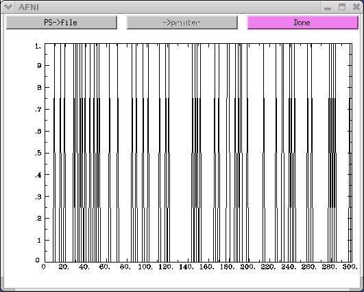 The x-axis on the above graph represents time. In this example, there are
300 time points along the x-axis. The y-axis represents the activity-rest
dichotomy. A time point with a "0" value indicates a rest period, while
a time point with a "1" value represents a stimulus presentation.
-----------------------
The random number 'seed' we have selected for this example (1234567) may
not necessarily produce the most optimal random order of our stimuli.
Therefore, it is wise to run 'RSFgen' several times, assigning a different
number seed each time. The "best" seed will be determined once we run
'3dDeconvolve' and statistically evaluate the quality of the stimulus timing
sequence that a particular seed generated (more on this topic in the
'3dDeconvolve' section that follows).
The easiest and least time-consuming way to run 'RSFgen' multiple times is
to introduce a 'foreach' loop to the command line. Recall from the
previous HowTo's that a 'foreach' loop is a UNIX command that implements a
loop where the loop variable takes on values from one or more lists.
For instance, the following 'foreach' loop can be added to our original
'RSFgen' command:
set seed = 1234567
foreach iter (`count -digits 3 1 100`)
RSFgen -nt 3 \
-num_stimts 3 \
-nreps 1 50 \
-nreps 2 50 \
-nreps 3 50 \
-seed ${seed} \
-prefix RSF.stim.${iter}.
@ seed = $seed + 1
end
-----------------------
* EXPLANATION of above commands:
set seed = 1234567 : 'seed' is a variable we have set, which represents the
number seed 1234567. There was no particular reason
why we chose this seed number except that it was easy
to type. In theory, the user can set the seed to any
number they desire.
foreach iter (`count -digits 3 1 100`)
: The 'count -digits 3 1 100' command produces the
numbers from 1 to 100, using 3 digits for each
number, i.e. 001 002 003 ... 099 100.
This particular foreach loop executes 100 times.
For each of those 100 iterations, the variable 'iter'
takes on the 3-digit value contained within the
parentheses, corresponding to the given iteration.
These 3-digit values of the 'iter' variable will be
used as part of the file name prefix passed to the
'RSFgen' program. 'RSFgen' will output files like:
RSF.stim.001.1.1D
RSF.stim.001.2.1D
RSF.stim.001.3.1D
RSF.stim.002.1.1D
RSF.stim.002.2.1D
RSF.stim.002.2.1D
.
.
.
RSF.stim.099.1.1D
RSF.stim.099.2.1D
RSF.stim.099.3.1D
RSF.stim.100.1.1D
RSF.stim.100.2.1D
RSF.stim.100.3.1D
The benefit of including this foreach loop in the
script is that one can choose to run hundreds, or even
thousands, of iterations of 'RSFgen' without having to
manually type in the command for each individual
iteration. The computer could simply be left to run
overnight without any human intervention.
@ seed = $seed + 1 : This command increases the random seed number by one
each time 'RSFgen' is executed. The first iteration
of RSFgen will begin with seed number 1234567 + 1 (or
1234568)
Iteration 1 - seed number = 1234567 + 1 = 1234568
Iteration 2 - seed number = 1234568 + 1 = 1234569
Iteration 3 - seed number = 1234569 + 1 = 1234570
. . . .
. . . .
. . . .
Iteration 98 - seed number = 1234664 + 1 = 1234665
Iteration 99 - seed number = 1234664 + 1 = 1234666
Iteration 100 - seed number = 1234665 + 1 = 1234667
end : This is the end of the foreach loop. Once the shell
reaches this statement, it goes back to the start of
the foreach loop and begins the next iteration. If
all iterations have been completed, the shell moves
on past this 'end' statement.
-----------------------
* 'RSFgen' as it appears in our '@stim_analyze' script:
To make this script more versatile, one can assign their own experiment
variables or parameters at the beginning of the script, using the UNIX
'set' command. These variables (e.g., length of the time series, number of
stimulus conditions, number of time points per condition, etc.) can be
customized to fit most experiment parameters. Our script '@stim_analyze'
contains the following default parameters:
set ts = 300
set stim = 3
set num_on = 50
set seed = 1234567
foreach iter (`count -digits 3 1 100`)
@ seed = $seed + 1
RSFgen -nt ${ts} \
-num_stimts ${stim} \
-nreps 1 $(num_on) \
-nreps 2 ${num_on} \
-nreps 3 ${num_on} \
-seed ${seed} \
-prefix RSF.stim.${iter}. >& /dev/null
* EXPLANATION of above commands:
set ts = 300 : The UNIX command 'set' allows the user to create a
variable that will be used throughout the script. The
first variable we have assigned for this script is
'ts', which refers to the length of the time series.
For this experiment,the overall time course will have
300 time points (i.e., 50 pictures + 50 words + 50
geometric figures + 150 'rest' periods).
set stim = 3 : 'stim' refers to the number of stimulus conditions in
the experiment. In this example, there are three:
(1) pictures, (2) words, and (3) geometric figures.
set num_on = 50 : 'num_on' refers to the number of time points per
stimulus condition. In this example, there are 50
time points (or 'on' events) for every stimulus
condition.
${<variable name>} : Whenever the set variable is used within the script,
it is encased in curly brackets and preceded by a '$'
symbol, e.g., ${ts}.
>& /dev/null : When a program is running, text often gets spit onto
the terminal window. Sometimes this output is not
interesting or relevant to most users. Therefore, one
can avoid viewing this text altogether by using the
'>' command to redirect it to a special 'trash' file
called /dev/null.
* NOTE: The script is set so that all stimulus timing files are stored
automatically in a newly created directory called 'stim_results'
(see 'Unix help - outdir' for more details).
----------------------------------------------------------------------------
----------------------------------------------------------------------------
* COMMAND: waver
Now that our random-order stimulus timing files have been generated, the
AFNI program 'waver' can be used to create an Ideal Reference Function
(IRF) for each stimulus timing file.
Usage: waver [-options] > output_filename
(see also 'waver -help')
-----------------------
EXAMPLE of 'waver' (from our script '@stim_analyze':)
waver -GAM -dt 1.0 -input RSF.stim.${iter}.1.1D > wav.hrf.${iter}.1.1D
waver -GAM -dt 1.0 -input RSF.stim.${iter}.2.1D > wav.hrf.${iter}.2.1D
waver -GAM -dt 1.0 -input RSF.stim.${iter}.3.1D > wav.hrf.${iter}.3.1D
-----------------------
Explanation of above waver options:
-GAM : This option specifies that waver will use the Gamma variate
waveform.
-dt 1.0 : This option tells waver to use 1.0 seconds for the delta time
(dt), which is the length of time between data points that are
output.
-input <infile> : This option allows waver to read the time series from the
specified 'RSF.stim.{$iter}.[1,2,3].1D' input files. These
input files will be convolved with the Gamma variate waveform
to produce the output files, 'wav.hrf.${iter}.[1,2,3].1D'.
-----------------------
The above command line will result in the creation of three ideal reference
functions for each 'RSFgen' iteration. Recall that we have specified 100
iterations of 'RSFgen' in our sample script. Therefore, there will be a
total of 300 IRF's (i.e., 100 for each of our 3 stimulus conditions):
wav.hrf.001.1.1D
wav.hrf.001.2.1D
wav.hrf.001.3.1D
wav.hrf.002.1.1D
wav.hrf.002.2.1D
wav.hrf.002.3.1D
.
.
.
wav.hrf.099.1.1D
wav.hrf.099.2.1D
wav.hrf.099.3.1D
wav.hrf.100.1.1D
wav.hrf.100.2.1D
wav.hrf.100.3.1D
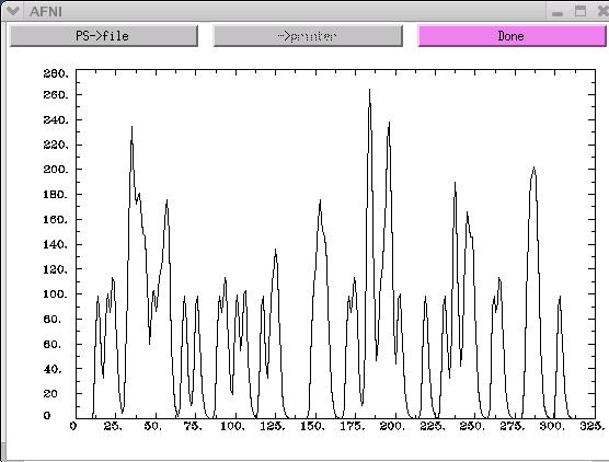
To view a graph of one of these files, simply run AFNI '1dplot'.
For example:
1dplot wav.hrf.001.1.1D
The x-axis on the above graph represents time. In this example, there are
300 time points along the x-axis. The y-axis represents the activity-rest
dichotomy. A time point with a "0" value indicates a rest period, while
a time point with a "1" value represents a stimulus presentation.
-----------------------
The random number 'seed' we have selected for this example (1234567) may
not necessarily produce the most optimal random order of our stimuli.
Therefore, it is wise to run 'RSFgen' several times, assigning a different
number seed each time. The "best" seed will be determined once we run
'3dDeconvolve' and statistically evaluate the quality of the stimulus timing
sequence that a particular seed generated (more on this topic in the
'3dDeconvolve' section that follows).
The easiest and least time-consuming way to run 'RSFgen' multiple times is
to introduce a 'foreach' loop to the command line. Recall from the
previous HowTo's that a 'foreach' loop is a UNIX command that implements a
loop where the loop variable takes on values from one or more lists.
For instance, the following 'foreach' loop can be added to our original
'RSFgen' command:
set seed = 1234567
foreach iter (`count -digits 3 1 100`)
RSFgen -nt 3 \
-num_stimts 3 \
-nreps 1 50 \
-nreps 2 50 \
-nreps 3 50 \
-seed ${seed} \
-prefix RSF.stim.${iter}.
@ seed = $seed + 1
end
-----------------------
* EXPLANATION of above commands:
set seed = 1234567 : 'seed' is a variable we have set, which represents the
number seed 1234567. There was no particular reason
why we chose this seed number except that it was easy
to type. In theory, the user can set the seed to any
number they desire.
foreach iter (`count -digits 3 1 100`)
: The 'count -digits 3 1 100' command produces the
numbers from 1 to 100, using 3 digits for each
number, i.e. 001 002 003 ... 099 100.
This particular foreach loop executes 100 times.
For each of those 100 iterations, the variable 'iter'
takes on the 3-digit value contained within the
parentheses, corresponding to the given iteration.
These 3-digit values of the 'iter' variable will be
used as part of the file name prefix passed to the
'RSFgen' program. 'RSFgen' will output files like:
RSF.stim.001.1.1D
RSF.stim.001.2.1D
RSF.stim.001.3.1D
RSF.stim.002.1.1D
RSF.stim.002.2.1D
RSF.stim.002.2.1D
.
.
.
RSF.stim.099.1.1D
RSF.stim.099.2.1D
RSF.stim.099.3.1D
RSF.stim.100.1.1D
RSF.stim.100.2.1D
RSF.stim.100.3.1D
The benefit of including this foreach loop in the
script is that one can choose to run hundreds, or even
thousands, of iterations of 'RSFgen' without having to
manually type in the command for each individual
iteration. The computer could simply be left to run
overnight without any human intervention.
@ seed = $seed + 1 : This command increases the random seed number by one
each time 'RSFgen' is executed. The first iteration
of RSFgen will begin with seed number 1234567 + 1 (or
1234568)
Iteration 1 - seed number = 1234567 + 1 = 1234568
Iteration 2 - seed number = 1234568 + 1 = 1234569
Iteration 3 - seed number = 1234569 + 1 = 1234570
. . . .
. . . .
. . . .
Iteration 98 - seed number = 1234664 + 1 = 1234665
Iteration 99 - seed number = 1234664 + 1 = 1234666
Iteration 100 - seed number = 1234665 + 1 = 1234667
end : This is the end of the foreach loop. Once the shell
reaches this statement, it goes back to the start of
the foreach loop and begins the next iteration. If
all iterations have been completed, the shell moves
on past this 'end' statement.
-----------------------
* 'RSFgen' as it appears in our '@stim_analyze' script:
To make this script more versatile, one can assign their own experiment
variables or parameters at the beginning of the script, using the UNIX
'set' command. These variables (e.g., length of the time series, number of
stimulus conditions, number of time points per condition, etc.) can be
customized to fit most experiment parameters. Our script '@stim_analyze'
contains the following default parameters:
set ts = 300
set stim = 3
set num_on = 50
set seed = 1234567
foreach iter (`count -digits 3 1 100`)
@ seed = $seed + 1
RSFgen -nt ${ts} \
-num_stimts ${stim} \
-nreps 1 $(num_on) \
-nreps 2 ${num_on} \
-nreps 3 ${num_on} \
-seed ${seed} \
-prefix RSF.stim.${iter}. >& /dev/null
* EXPLANATION of above commands:
set ts = 300 : The UNIX command 'set' allows the user to create a
variable that will be used throughout the script. The
first variable we have assigned for this script is
'ts', which refers to the length of the time series.
For this experiment,the overall time course will have
300 time points (i.e., 50 pictures + 50 words + 50
geometric figures + 150 'rest' periods).
set stim = 3 : 'stim' refers to the number of stimulus conditions in
the experiment. In this example, there are three:
(1) pictures, (2) words, and (3) geometric figures.
set num_on = 50 : 'num_on' refers to the number of time points per
stimulus condition. In this example, there are 50
time points (or 'on' events) for every stimulus
condition.
${<variable name>} : Whenever the set variable is used within the script,
it is encased in curly brackets and preceded by a '$'
symbol, e.g., ${ts}.
>& /dev/null : When a program is running, text often gets spit onto
the terminal window. Sometimes this output is not
interesting or relevant to most users. Therefore, one
can avoid viewing this text altogether by using the
'>' command to redirect it to a special 'trash' file
called /dev/null.
* NOTE: The script is set so that all stimulus timing files are stored
automatically in a newly created directory called 'stim_results'
(see 'Unix help - outdir' for more details).
----------------------------------------------------------------------------
----------------------------------------------------------------------------
* COMMAND: waver
Now that our random-order stimulus timing files have been generated, the
AFNI program 'waver' can be used to create an Ideal Reference Function
(IRF) for each stimulus timing file.
Usage: waver [-options] > output_filename
(see also 'waver -help')
-----------------------
EXAMPLE of 'waver' (from our script '@stim_analyze':)
waver -GAM -dt 1.0 -input RSF.stim.${iter}.1.1D > wav.hrf.${iter}.1.1D
waver -GAM -dt 1.0 -input RSF.stim.${iter}.2.1D > wav.hrf.${iter}.2.1D
waver -GAM -dt 1.0 -input RSF.stim.${iter}.3.1D > wav.hrf.${iter}.3.1D
-----------------------
Explanation of above waver options:
-GAM : This option specifies that waver will use the Gamma variate
waveform.
-dt 1.0 : This option tells waver to use 1.0 seconds for the delta time
(dt), which is the length of time between data points that are
output.
-input <infile> : This option allows waver to read the time series from the
specified 'RSF.stim.{$iter}.[1,2,3].1D' input files. These
input files will be convolved with the Gamma variate waveform
to produce the output files, 'wav.hrf.${iter}.[1,2,3].1D'.
-----------------------
The above command line will result in the creation of three ideal reference
functions for each 'RSFgen' iteration. Recall that we have specified 100
iterations of 'RSFgen' in our sample script. Therefore, there will be a
total of 300 IRF's (i.e., 100 for each of our 3 stimulus conditions):
wav.hrf.001.1.1D
wav.hrf.001.2.1D
wav.hrf.001.3.1D
wav.hrf.002.1.1D
wav.hrf.002.2.1D
wav.hrf.002.3.1D
.
.
.
wav.hrf.099.1.1D
wav.hrf.099.2.1D
wav.hrf.099.3.1D
wav.hrf.100.1.1D
wav.hrf.100.2.1D
wav.hrf.100.3.1D
To view a graph of one of these files, simply run AFNI '1dplot'.
For example:
1dplot wav.hrf.001.1.1D
 * NOTE: The script is set so that all IRF files are stored automatically in
a newly created directory called 'stim_results'.
----------------------------------------------------------------------------
----------------------------------------------------------------------------
* COMMAND: 3dDeconvolve (with the -nodata option)
With so many stimulus functions created by the 100 iterations of 'RSF_gen',
how do we determine which randomized order of stimulus events is most
optimal? That is, which randomized stimulus timing sequence results in the
most ideal reference functions that are easiest to deconvolve? Proper
deconvolution is especially important in rapid event-related designs
where the inter-stimulus interval between trials is only a few seconds,
resulting in large overlapping of the hemodynamic response functions.
In HowTo #2, '3dDeconvolve' was used to perform a multiple linear
regression using multiple input stimulus time series. A 3D+time dataset
was used as input for the deconvolution program, and the output was a
'bucket' dataset, consisting of various parameters of interest such as the
F-statistic for significance of the estimated impulse response.
In this HowTo, '3dDeconvolve' will be used to evaluate an experimental
design PRIOR to collecting data. This is done by using the '-nodata'
option in place of the '-input' command. The '-nodata' option is used to
specify that there is no input data, only input stimulus functions.
Usage:
(Note: Mandatory arguments are shown below without brackets;
optional arguments are encased within the square brackets.)
3dDeconvolve
-nodata
[-nfirst <fnumber>]
[-nlast <lnumber>]
[-polort <pnumber>]
-num_stimts <number>
-stim_file <k sname>
-stim_label <k slabel>
[-glt <s glt_name>]
(see also '3dDeconvolve -help')
* NOTE: Due to the large number of options in '3dDeconvolve', it is HIGHLY
recommended that the '3dDeconvolve' command be written into a script
using a text editor, which can then be executed in the UNIX window.
-----------------------
EXAMPLE of '3dDeconvolve' with the '-nodata' option
(as it appears in our script '@stim_analyze'):
3dDeconvolve \
-nodata \
-nfirst 4 \
-nlast 299 \
-polort 1 \
-num_stimts ${stim} \
-stim_file 1 "wav.hrf.${iter}.1.1D" \
-stim_label 1 "stim_A" \
-stim_file 2 "wav.hrf.${iter}.2.1D" \
-stim_label 2 "stim_B" \
-stim_file 3 "wav.hrf.${iter}.3.1D" \
-stim_label 3 "stim_C" \
-glt 1 contrasts/contrast_AB \
-glt 1 contrasts/contrast_AC \
-glt 1 contrasts/contrast_BC \
> 3dD.nodata.${iter}
* NOTE: Contrast files are needed to do general linear tests (GLTs).
In our example, we have three contrast files located in a
directory called 'contrasts'. Each contrast file consists of a
matrix of 0's, 1's, and -1's.
To run the GLT, the contrast file must specify the coefficient
of the linear combinations the user wants to test against zero.
For instance, contrast AB is examining significant differences
between voxel activation during picture presentations versus word
presentations. As such, the matrix for 'contrast_AB' would look
like this:
0 0 1 -1 0
The first two zero's signify the baseline parameters, both of
which are to be ignored in this GLT. The 1 and -1 tells
'3dDeconvolve' to run the GLT between pictures and words. The
final zero represents the third variable in our study - geometric
shapes - which is to be ignored in this particular contrast.
-----------------------
Explanation of above '3dDeconvolve' options.
-nodata : This option (which replaces the '-input' option) allows the
user to evaluate the experimental design without entering any
measurement data. The user must specify the input stimulus
functions.
-nfirst/-nlast : The length of the 3D+time dataset (i.e., the number of time
points in our experiment) must be specified using the
'-nfirst' and '-nlast' options. Recall that we have 300
times points in our hypothetical study.
'-nfirst = 4' and '-nlast = 299' indicate that the first
four time points (0, 1, 2, 3) are to be omitted from our
experiment evaluation. Since the time point counting starts
with 0, 299 is the last time point. Removal of the first
few time points in a time series is typically done because
it takes 4-8 seconds for the scanner to reach steady state.
The first few images are much brighter than the rest, so
their inclusion damages the statistical analysis.
-stim_file : This option is used to specify the name of each ideal
reference function file. Recall that in our hypothetical
study, for each of our 100 iterations we have 3 IRF files,
one for each condition. These 3 IRF files will be used in
'3dDeconvolve' and will be specified using 3 '-stim_file'
options.
-stim_label <k> : To keep track of our stimulus conditions, organization and
proper labeling are essential. This option is a handy tool
that provides a label for the output corresponding to the kth
input stimulus function:
Pictures : -stim_file 1 "stim_A"
Words : -stim_file 2 "stim_B"
Geometric figures : -stim_file 3 "stim_C"
> 3dD.nodata.${iter} :
This option informs '3dDeconvolve' to redirect the resulting
data from the general linear tests into output files that will
be labeled '3dD.nodata.${iter}. Since the ${iter} variable
represents the 100 iterations we have specified in our script,
there will be 100 of these '3dD.nodata...' output files:
3dD.nodata.001
3dD.nodata.002
3dD.nodata.003
.
.
.
3dD.nodata.098
3dD.nodata.099
3dD.nodata.100
* NOTE: The script is set so that all '3dD.nodata.{$iter}' files are stored
automatically in a newly created directory called 'stim_results'.
-----------------------
At this point, you may be asking:
"What information will these '3dD.nodata.{$iter}' output files contain
and how will they help me evaluate the quality of our 300 ideal
reference functions?"
One way to answer this question is to actually open one of these files and
view the information within. For instance, the output file '3dD.nodata.001'
contains the following data:
Program: 3dDeconvolve
Author: B. Douglas Ward
Initial Release: 02 September 1998
Latest Revision: 02 December 2002
(X'X) inverse matrix:
0.0341 -0.0001 -0.0001 -0.0001 -0.0001
-0.0001 0.0000 -0.0000 0.0000 0.0000
-0.0001 -0.0000 0.0000 0.0000 0.0000
-0.0001 0.0000 0.0000 0.0000 0.0000
-0.0001 0.0000 0.0000 0.0000 0.0000
Stimulus: stim_A
h[ 0] norm. std. dev. = 0.0010
Stimulus: stim_B
h[ 0] norm. std. dev. = 0.0009
Stimulus: stim_C
h[ 0] norm. std. dev. = 0.0011
General Linear Test: GLT #1
LC[0] norm. std. dev. = 0.0013
General Linear Test: GLT #2
LC[0] norm. std. dev. = 0.0012
General Linear Test: GLT #3
LC[0] norm. std. dev. = 0.0013
-----------------------
What do all of these statistics mean?
Specifically, what is a normalized standard deviation?
First, recall that the output from '3dD.nodata.001' stems from the stimulus
timing files we created way back with 'RSFgen'. Specifically,
(1) number seed 1234568 generated a specific randomized sequence of our
stimulus events.
(2) these stimulus timing files were then convolved with a waveform
(using AFNI 'waver') to create ideal reference functions.
* The Normalized Standard Deviation (a quick explanation):
In a nutshell, the normalized standard deviation is the square root of the
measurement error variance. Since this variance is unknown, we estimate it
with the Mean Square Error (MSE). A smaller normalized standard deviation
indicates a smaller MSE. A small MSE is desirable, because MSE relates to
the unexplained portion of the variance. Unexplained variance is NOT good.
Therefore, the smaller the MSE (or normalized standard deviation), the better.
Our goal is to find that particular '3dD.nodata.{$iter}' file that contains
the smallest normalized standard deviations. This file will lead us to the
number seed that generated the randomized stimulus timing files, that
resulted in overlapping hemodynamic responses that were deconvolved with
the least amount of unexplained variance. THIS IS A GOOD THING!
-----------------------
In the above example, the variances from our general linear tests are
0.0013, 0.0012, and 0.0013. If the variances for all three general linear
tests (GLTs) were combined, the sum would be 0.0038:
GLT#1 (contrast AB): norm. std. dev. = .0013
GLT#2 (contrast AC): norm. std. dev. = .0012
GLT#3 (contrast BC): norm. std. dev. = .0013
SUM = .0038
.0038 seems pretty low (i.e., not too much unexplained variance).
However, is there another seed number that generates a stimulus timing
sequence that elicits an even smaller sum of the variances? To determine
this, we much look through all 100 of our '3dD.nodata.{$iter}' files and
calculate the sum of the variances from our 3 GLTs.
However, going through all 100 '3dD.nodata.{$iter}' files is cumbersome and
time consuming. Fortunately, our script '@stim_analyze' is set up to
automatically add the three GLT norm. std. deviations from each
'3dD.nodata.{$iter}' file, and append that information into a single file
called 'LC_sums'. We can then peruse this file and locate the number seed
that resulted in the smallest sum of the variances.
The 'LC_sums' file will be stored in the 'stim_results' directory, along
with all the other files we have created up to this point.
Once the script is run and the file 'LC_sums' is created, it can be opened
to display the following information. Use the UNIX 'more' command to view
the file in the terminal window. Scroll down by pressing the space bar:
more stim_results/LC_sums
Result: 38 = 13 + 12 + 13 : iteration 001, seed 1234568
36 = 12 + 12 + 12 : iteration 002, seed 1234569
37 = 12 + 13 + 12 : iteration 003, seed 1234570
38 = 12 + 13 + 13 : iteration 004, seed 1234571
38 = 12 + 14 + 12 : iteration 005, seed 1234572
.
.
.
37 = 13 + 11 + 13 : iteration 096, seed 1234663
37 = 13 + 12 + 12 : iteration 097, seed 1234664
40 = 13 + 14 + 13 : iteration 098, seed 1234665
37 = 12 + 12 + 13 : iteration 099, seed 1234666
37 = 11 + 13 + 13 : iteration 100, seed 1234667
* NOTE: Since the UNIX shell can only do computations on integers, the
decimals have been removed. For example, .0013+.0012+.0013 has
been replaced with 13+12+13. Either way, we are looking for the
smallest sum of the variances.
-----------------------
The user can SORT the file 'LC_sums' by the first column of data, which
in this case, happens to be the sum of the variances. To sort, type the
following command in the shell:
sort stim_results/LC_sums
Result: 33 = 11 + 11 + 11 : iteration 039, seed 1234606
33 = 11 + 11 + 11 : iteration 078, seed 1234645
33 = 12 + 10 + 11 : iteration 025, seed 1234592
34 = 10 + 12 + 12 : iteration 037, seed 1234604
34 = 11 + 11 + 12 : iteration 031, seed 1234598
.
.
.
41 = 13 + 15 + 13 : iteration 008, seed 1234575
41 = 13 + 15 + 13 : iteration 061, seed 1234628
41 = 14 + 14 + 13 : iteration 015, seed 1234582
42 = 15 + 12 + 15 : iteration 058, seed 1234625
42 = 15 + 13 + 14 : iteration 040, seed 1234607
Instead of viewing the entire file, the user can choose to view only the
number seed that elicited the smallest sum of the variances. To do this,
the user must first sort the file (just like we did above), and then
pipe (|) the result to the UNIX 'head' utility, which will display only the
first line of the sorted file:
sort stim_results/LC_sums | head -1
Result: 33 = 11 + 11 + 11 : iteration 039, seed 1234606
FINALLY, we have found the number seed that resulted in the smallest
sum of the variances obtained from our general linear tests. Seed number
1234606 (iteration #039) generated the randomized stimulus timing files
that resulted in overlapping hemodynamic responses that were deconvolved
with the least amount of unexplained variance, thus increasing our
statistical power.
Since the stimulus timing files that correspond to this seed are from
iteration #039, the files are as follows, located in the stim_results
directory:
RSF.stim.039.1.1D
RSF.stim.039.2.1D
RSF.stim.039.3.1D
* NOTE: This number seed is the best one from the 100 number seeds included
in our script. It may not necessarily be the best number seed overall.
There may be a number seed out there we did not use, which results in an
even smaller amount of unexplained variance. Luckily, with a script, it
becomes quite easy to increase the seed number generation from 100
iterations to 1000, 100,000, or even 1,000,000 iterations. It is up to
the user to decide how many iterations of 'RSFgen' are necessary.
However, be aware that each iteration results in three stimulus timing
files, which are then convolved with a waveform in 'waver' to create
three IRF files. Therefore, one iteration results in six output files.
This can add up. 1000 iterations will result in 6000 output files and
100,000 iterations will result in 600,000 output files!
-----------------------
-----------------------
** FINAL NOTE:
Proper research design and experiment evaluation does require some serious
time and planning. However, it pales in comparison to the amount of time,
effort, and resources that are wasted on poorly designed experiments, which
result in low statistical power and cloudy results. Fortunately, the script
presented in this HowTo can serve to expedite the evaluation process and
get your study up and running in no time. So with that we conclude this
third HowTo.
GOOD LUCK and HAPPY SCANNING!
* NOTE: The script is set so that all IRF files are stored automatically in
a newly created directory called 'stim_results'.
----------------------------------------------------------------------------
----------------------------------------------------------------------------
* COMMAND: 3dDeconvolve (with the -nodata option)
With so many stimulus functions created by the 100 iterations of 'RSF_gen',
how do we determine which randomized order of stimulus events is most
optimal? That is, which randomized stimulus timing sequence results in the
most ideal reference functions that are easiest to deconvolve? Proper
deconvolution is especially important in rapid event-related designs
where the inter-stimulus interval between trials is only a few seconds,
resulting in large overlapping of the hemodynamic response functions.
In HowTo #2, '3dDeconvolve' was used to perform a multiple linear
regression using multiple input stimulus time series. A 3D+time dataset
was used as input for the deconvolution program, and the output was a
'bucket' dataset, consisting of various parameters of interest such as the
F-statistic for significance of the estimated impulse response.
In this HowTo, '3dDeconvolve' will be used to evaluate an experimental
design PRIOR to collecting data. This is done by using the '-nodata'
option in place of the '-input' command. The '-nodata' option is used to
specify that there is no input data, only input stimulus functions.
Usage:
(Note: Mandatory arguments are shown below without brackets;
optional arguments are encased within the square brackets.)
3dDeconvolve
-nodata
[-nfirst <fnumber>]
[-nlast <lnumber>]
[-polort <pnumber>]
-num_stimts <number>
-stim_file <k sname>
-stim_label <k slabel>
[-glt <s glt_name>]
(see also '3dDeconvolve -help')
* NOTE: Due to the large number of options in '3dDeconvolve', it is HIGHLY
recommended that the '3dDeconvolve' command be written into a script
using a text editor, which can then be executed in the UNIX window.
-----------------------
EXAMPLE of '3dDeconvolve' with the '-nodata' option
(as it appears in our script '@stim_analyze'):
3dDeconvolve \
-nodata \
-nfirst 4 \
-nlast 299 \
-polort 1 \
-num_stimts ${stim} \
-stim_file 1 "wav.hrf.${iter}.1.1D" \
-stim_label 1 "stim_A" \
-stim_file 2 "wav.hrf.${iter}.2.1D" \
-stim_label 2 "stim_B" \
-stim_file 3 "wav.hrf.${iter}.3.1D" \
-stim_label 3 "stim_C" \
-glt 1 contrasts/contrast_AB \
-glt 1 contrasts/contrast_AC \
-glt 1 contrasts/contrast_BC \
> 3dD.nodata.${iter}
* NOTE: Contrast files are needed to do general linear tests (GLTs).
In our example, we have three contrast files located in a
directory called 'contrasts'. Each contrast file consists of a
matrix of 0's, 1's, and -1's.
To run the GLT, the contrast file must specify the coefficient
of the linear combinations the user wants to test against zero.
For instance, contrast AB is examining significant differences
between voxel activation during picture presentations versus word
presentations. As such, the matrix for 'contrast_AB' would look
like this:
0 0 1 -1 0
The first two zero's signify the baseline parameters, both of
which are to be ignored in this GLT. The 1 and -1 tells
'3dDeconvolve' to run the GLT between pictures and words. The
final zero represents the third variable in our study - geometric
shapes - which is to be ignored in this particular contrast.
-----------------------
Explanation of above '3dDeconvolve' options.
-nodata : This option (which replaces the '-input' option) allows the
user to evaluate the experimental design without entering any
measurement data. The user must specify the input stimulus
functions.
-nfirst/-nlast : The length of the 3D+time dataset (i.e., the number of time
points in our experiment) must be specified using the
'-nfirst' and '-nlast' options. Recall that we have 300
times points in our hypothetical study.
'-nfirst = 4' and '-nlast = 299' indicate that the first
four time points (0, 1, 2, 3) are to be omitted from our
experiment evaluation. Since the time point counting starts
with 0, 299 is the last time point. Removal of the first
few time points in a time series is typically done because
it takes 4-8 seconds for the scanner to reach steady state.
The first few images are much brighter than the rest, so
their inclusion damages the statistical analysis.
-stim_file : This option is used to specify the name of each ideal
reference function file. Recall that in our hypothetical
study, for each of our 100 iterations we have 3 IRF files,
one for each condition. These 3 IRF files will be used in
'3dDeconvolve' and will be specified using 3 '-stim_file'
options.
-stim_label <k> : To keep track of our stimulus conditions, organization and
proper labeling are essential. This option is a handy tool
that provides a label for the output corresponding to the kth
input stimulus function:
Pictures : -stim_file 1 "stim_A"
Words : -stim_file 2 "stim_B"
Geometric figures : -stim_file 3 "stim_C"
> 3dD.nodata.${iter} :
This option informs '3dDeconvolve' to redirect the resulting
data from the general linear tests into output files that will
be labeled '3dD.nodata.${iter}. Since the ${iter} variable
represents the 100 iterations we have specified in our script,
there will be 100 of these '3dD.nodata...' output files:
3dD.nodata.001
3dD.nodata.002
3dD.nodata.003
.
.
.
3dD.nodata.098
3dD.nodata.099
3dD.nodata.100
* NOTE: The script is set so that all '3dD.nodata.{$iter}' files are stored
automatically in a newly created directory called 'stim_results'.
-----------------------
At this point, you may be asking:
"What information will these '3dD.nodata.{$iter}' output files contain
and how will they help me evaluate the quality of our 300 ideal
reference functions?"
One way to answer this question is to actually open one of these files and
view the information within. For instance, the output file '3dD.nodata.001'
contains the following data:
Program: 3dDeconvolve
Author: B. Douglas Ward
Initial Release: 02 September 1998
Latest Revision: 02 December 2002
(X'X) inverse matrix:
0.0341 -0.0001 -0.0001 -0.0001 -0.0001
-0.0001 0.0000 -0.0000 0.0000 0.0000
-0.0001 -0.0000 0.0000 0.0000 0.0000
-0.0001 0.0000 0.0000 0.0000 0.0000
-0.0001 0.0000 0.0000 0.0000 0.0000
Stimulus: stim_A
h[ 0] norm. std. dev. = 0.0010
Stimulus: stim_B
h[ 0] norm. std. dev. = 0.0009
Stimulus: stim_C
h[ 0] norm. std. dev. = 0.0011
General Linear Test: GLT #1
LC[0] norm. std. dev. = 0.0013
General Linear Test: GLT #2
LC[0] norm. std. dev. = 0.0012
General Linear Test: GLT #3
LC[0] norm. std. dev. = 0.0013
-----------------------
What do all of these statistics mean?
Specifically, what is a normalized standard deviation?
First, recall that the output from '3dD.nodata.001' stems from the stimulus
timing files we created way back with 'RSFgen'. Specifically,
(1) number seed 1234568 generated a specific randomized sequence of our
stimulus events.
(2) these stimulus timing files were then convolved with a waveform
(using AFNI 'waver') to create ideal reference functions.
* The Normalized Standard Deviation (a quick explanation):
In a nutshell, the normalized standard deviation is the square root of the
measurement error variance. Since this variance is unknown, we estimate it
with the Mean Square Error (MSE). A smaller normalized standard deviation
indicates a smaller MSE. A small MSE is desirable, because MSE relates to
the unexplained portion of the variance. Unexplained variance is NOT good.
Therefore, the smaller the MSE (or normalized standard deviation), the better.
Our goal is to find that particular '3dD.nodata.{$iter}' file that contains
the smallest normalized standard deviations. This file will lead us to the
number seed that generated the randomized stimulus timing files, that
resulted in overlapping hemodynamic responses that were deconvolved with
the least amount of unexplained variance. THIS IS A GOOD THING!
-----------------------
In the above example, the variances from our general linear tests are
0.0013, 0.0012, and 0.0013. If the variances for all three general linear
tests (GLTs) were combined, the sum would be 0.0038:
GLT#1 (contrast AB): norm. std. dev. = .0013
GLT#2 (contrast AC): norm. std. dev. = .0012
GLT#3 (contrast BC): norm. std. dev. = .0013
SUM = .0038
.0038 seems pretty low (i.e., not too much unexplained variance).
However, is there another seed number that generates a stimulus timing
sequence that elicits an even smaller sum of the variances? To determine
this, we much look through all 100 of our '3dD.nodata.{$iter}' files and
calculate the sum of the variances from our 3 GLTs.
However, going through all 100 '3dD.nodata.{$iter}' files is cumbersome and
time consuming. Fortunately, our script '@stim_analyze' is set up to
automatically add the three GLT norm. std. deviations from each
'3dD.nodata.{$iter}' file, and append that information into a single file
called 'LC_sums'. We can then peruse this file and locate the number seed
that resulted in the smallest sum of the variances.
The 'LC_sums' file will be stored in the 'stim_results' directory, along
with all the other files we have created up to this point.
Once the script is run and the file 'LC_sums' is created, it can be opened
to display the following information. Use the UNIX 'more' command to view
the file in the terminal window. Scroll down by pressing the space bar:
more stim_results/LC_sums
Result: 38 = 13 + 12 + 13 : iteration 001, seed 1234568
36 = 12 + 12 + 12 : iteration 002, seed 1234569
37 = 12 + 13 + 12 : iteration 003, seed 1234570
38 = 12 + 13 + 13 : iteration 004, seed 1234571
38 = 12 + 14 + 12 : iteration 005, seed 1234572
.
.
.
37 = 13 + 11 + 13 : iteration 096, seed 1234663
37 = 13 + 12 + 12 : iteration 097, seed 1234664
40 = 13 + 14 + 13 : iteration 098, seed 1234665
37 = 12 + 12 + 13 : iteration 099, seed 1234666
37 = 11 + 13 + 13 : iteration 100, seed 1234667
* NOTE: Since the UNIX shell can only do computations on integers, the
decimals have been removed. For example, .0013+.0012+.0013 has
been replaced with 13+12+13. Either way, we are looking for the
smallest sum of the variances.
-----------------------
The user can SORT the file 'LC_sums' by the first column of data, which
in this case, happens to be the sum of the variances. To sort, type the
following command in the shell:
sort stim_results/LC_sums
Result: 33 = 11 + 11 + 11 : iteration 039, seed 1234606
33 = 11 + 11 + 11 : iteration 078, seed 1234645
33 = 12 + 10 + 11 : iteration 025, seed 1234592
34 = 10 + 12 + 12 : iteration 037, seed 1234604
34 = 11 + 11 + 12 : iteration 031, seed 1234598
.
.
.
41 = 13 + 15 + 13 : iteration 008, seed 1234575
41 = 13 + 15 + 13 : iteration 061, seed 1234628
41 = 14 + 14 + 13 : iteration 015, seed 1234582
42 = 15 + 12 + 15 : iteration 058, seed 1234625
42 = 15 + 13 + 14 : iteration 040, seed 1234607
Instead of viewing the entire file, the user can choose to view only the
number seed that elicited the smallest sum of the variances. To do this,
the user must first sort the file (just like we did above), and then
pipe (|) the result to the UNIX 'head' utility, which will display only the
first line of the sorted file:
sort stim_results/LC_sums | head -1
Result: 33 = 11 + 11 + 11 : iteration 039, seed 1234606
FINALLY, we have found the number seed that resulted in the smallest
sum of the variances obtained from our general linear tests. Seed number
1234606 (iteration #039) generated the randomized stimulus timing files
that resulted in overlapping hemodynamic responses that were deconvolved
with the least amount of unexplained variance, thus increasing our
statistical power.
Since the stimulus timing files that correspond to this seed are from
iteration #039, the files are as follows, located in the stim_results
directory:
RSF.stim.039.1.1D
RSF.stim.039.2.1D
RSF.stim.039.3.1D
* NOTE: This number seed is the best one from the 100 number seeds included
in our script. It may not necessarily be the best number seed overall.
There may be a number seed out there we did not use, which results in an
even smaller amount of unexplained variance. Luckily, with a script, it
becomes quite easy to increase the seed number generation from 100
iterations to 1000, 100,000, or even 1,000,000 iterations. It is up to
the user to decide how many iterations of 'RSFgen' are necessary.
However, be aware that each iteration results in three stimulus timing
files, which are then convolved with a waveform in 'waver' to create
three IRF files. Therefore, one iteration results in six output files.
This can add up. 1000 iterations will result in 6000 output files and
100,000 iterations will result in 600,000 output files!
-----------------------
-----------------------
** FINAL NOTE:
Proper research design and experiment evaluation does require some serious
time and planning. However, it pales in comparison to the amount of time,
effort, and resources that are wasted on poorly designed experiments, which
result in low statistical power and cloudy results. Fortunately, the script
presented in this HowTo can serve to expedite the evaluation process and
get your study up and running in no time. So with that we conclude this
third HowTo.
GOOD LUCK and HAPPY SCANNING!