HOW-TO #5
Across-Subjects Comparisons of FMRI Data -
Running Analysis of Variance (ANOVA) with AFNI 3DANOVA Programs
PART I: Preparing Subject Data for ANOVA
Outline of AFNI How-To #5, PART I:
---------------------------------
I. Very Quick Introduction to our Sample Study
II. Process Individual Subjects' Data First
A. Create anatomical datasets with AFNI 'to3d'.
B. Transfer anatomical datasets to Talairach coordinates.
C. Process time series datasets with AFNI 'Imon' (or 'Ifile').
D. Volume Register and shift the voxel time series from each 3D+time
dataset (10 runs per subject) with AFNI '3dvolreg'
E. Smooth each 3D+time dataset with AFNI '3dmerge'.
F. Normalize each 3D+time Dataset:
1) Why Bother Normalizing the Data?
2) Clip the anatomical dataset so that background regions are set
to zero with AFNI '3dClipLevel'.
3) Calculate mean baseline for each run with AFNI '3dTstat'.
4) Compute percent change for each run with AFNI '3dcalc'.
G. Concatenate our 10 3D+time runs with AFNI '3dTcat'
H. Run deconvolution analysis for each subject with AFNI '3dDeconvolve'.
I. "Slim down" a bucket dataset with AFNI '3dbucket'.
J. Use AFNI '3dTstat' to remove time lags from our IRF datasets and
average the remaining lags
K. Use AFNI 'adwarp' to resample functional datasets to same grid as our
Talairached anatomical datasets.
------------------------------------------------------------------------------
------------------------------------------------------------------------------
I. VERY QUICK INTRODUCTION TO OUR SAMPLE STUDY
------------------------------------------------------------------------------
------------------------------------------------------------------------------
The following experiment will serve as our sample study:
Experiment:
FMRI and complex visual motion.
Design:
Event-related
Conditions:
1. Human Movie (HM)
2. Tool Movie (TM)
3. Human Point Light (HP)
4. Tool Point Light (TP)
Data Collected:
One anatomical, spoiled grass dataset for each participant, consisting
of 124 sagittal slices.
Ten functional, echo-planar datasets for each participant, consisting of
23 axial slices, 138 volumes in each slice. TR is set to 2 seconds.
For more information on this experiment, see the 'Background: The Experiment'
section of this how-to or refer to:
Beauchamp, M.S., Lee, K.E., Haxby, J. V., & Martin, A. (2003). FMRI
responses to video and point-light displays of moving humans and
manipulable objects. Journal of Cognitive Neuroscience, 15:7,
991-1001.
-----------------------------------------------------------------------------
-----------------------------------------------------------------------------
II. PROCESS INDIVIDUAL SUBJECTS' DATA FIRST
-----------------------------------------------------------------------------
-----------------------------------------------------------------------------
NOTE:
----
For your convenience, we have already processed steps II.A - II.C for you. That
is, we have created anatomical datasets for each subject (step II.A) and
transformed them to Talairach coordinates (step II.B). We have also processed
the time-series data (step II.C) so that there are ten 3D+time datasets per
subject. These datasets can be found in each subject's directory.
These preliminary steps were done for you because with 10 runs of data that
contain 23 volumes, 138 time points each, we would have 31,740 I-files! The tar
file we would have to create with all of this data would simply be too big and
cumbersome for you to download. Therefore, we have already created the datasets
for you with AFNI, and simply provide an explanation of what we did in Steps
II.A-II.C below. If you are intent on starting off with the raw image files,
these data can be downloaded from the fMRI Data Center archive at www.fmridc.org.
The accession number is 2-2003-113QA (donated by Michael Beauchamp).
The script that accompanies this how-to begins with step II.D:
"Volume Register and shift the voxel time series from each 3D+time
dataset with AFNI '3dvolreg'"
-----------------------------------------------------------------------------
A. Create Anatomical Datasets with AFNI 'to3d'
-------------------------------------------
COMMAND: to3d
This program is used to create 3D datasets from individual image files.
Usage: to3d -prefix [pname] File list
(see also 'to3d -help)
The program 'to3d' has been described in full detail in How-to's #1 and #2.
To simply reiterate, 'to3d' is used to convert individual image files into
three-dimensional volumes in AFNI.
For our sample experiment, the anatomical data consisted of 124 sagittal
slices for each subject (ASL orientation, 256x256 voxel matrix, 1.2 mm
slice thickness). The following command was used to create an anatomical
dataset for each subject:
foreach subj (ED EE EF)
to3d -prefix {$subj}spgr+orig I.*
end
We have already completed this step for you - the resulting datasets are
shown below and stored in each subject's directory. For example:
cd Points/ED/ cd Points/EE/ cd Points/EF/
ls ls ls
EDspgr+orig.HEAD EEspgr+orig.HEAD EFspgr+orig.HEAD
EDspgr+orig.BRIK EEspgr+orig.BRIK EFspgr+orig.BRIK
----------------------------------------------------------------------------
----------------------------------------------------------------------------
B. Transfer Anatomical Datasets to Talairach Coordinates
-----------------------------------------------------
Once the anatomical volumes for each subject are created, they must be
transformed into Talairach space. In AFNI, this step must be done
manually. There is no command line program or plugin yet (but coming
soon!) that will automatically do the transformation for you. Detailed
instructions regarding Talairach transformation can be found on the AFNI
website http://afni.nimh.nih.gov, under "AFNI - Documentation - Edu -
Class Notes - Lecture 8: Transforming Datasets to Talairach-Tourneaux
Coordinates."
For our sample study, we have already completed this step for you. The
transformed datasets have the same prefix (e.g., 'EDspgr' for subject ED)
as the original, un-Talairached datasets, but the "view" has been switched
from 'orig' to 'tlrc' (which is short for "Talairach"). AFNI automatically
changes the "view" whenever an ac-pc alignment or Talairach transformation
has been done. For example:
cd Points/ED/ cd Points/EE/ cd Points/EF/
EDspgr+tlrc.HEAD EEspgr+tlrc.HEAD EFspgr+tlrc.HEAD
EDspgr+tlrc.BRIK EEspgr+tlrc.BRIK EFspgr+tlrc.BRIK
With the anatomical datasets completed, we can proceed with creating
datasets for our echo planar images.
----------------------------------------------------------------------------
----------------------------------------------------------------------------
C. Process Time Series Datasets with AFNI 'Imon'
--------------------------------------------
COMMAND: Imon
Use AFNI 'Imon' to locate any missing or out-of-sequence image files.
Include the '-GERT_Reco2' option on the command line to create 3D+time
AFNI datasets from the time series data.
Usage: Imon [options] -start_dir DIR
(see also 'Imon -help')
In this sample study, 10 echo planar runs were obtained for each subject.
As described in gross detail in how-to #1, AFNI 'I-file' is a handy program
to use when dealing with multiple runs of data. First, 'I-file' will
determine where one EPI run ends and the next one begins. After this
initial step, 'Ifile' calls a script that creates the AFNI bricks for each
run.
Instead of 'Ifile', another option is to use an AFNI program called 'Imon'.
'Imon' is usually used to examine the integrity of I-files. For instance,
the program will notify the user of any missing slice or any slice that is
acquired out of order. However, 'Imon' can also be used to create AFNI
datasets if the '-GERT_Reco2' option is specified on the command line.
In our sample study, each subject has 10 runs of data. Each run consists
of 138 volumes, 23 axial slices each (i.e., 138 x 23 = 3174 I-files per
run). The axis orientation is RAS, each slice is a 64x64 voxel matrix, the
slice thickness is 5.0mm, and the TR = 2 seconds. Recall from previous
how-to's that EPI images collected using GE's Real Time (GERT) EPI sequence
are saved in a peculiar fashion. Only 999 image files can be saved in each
folder (or directory). In this example, the 3174 I-files in each run would
be dispersed over 3 entire directories, plus part of a fourth one. As such,
our 10 runs of data are dispersed over 32 directories! The directories are
labeled by numbers - starting with 003/ - and increase by increments of 20
(GE does this by default). For instance:
003/ 023/ 043/ 063/ 083/ 103/ 123/ ... 623/
For our sample experiment, the following command was run for each subject:
Imon -GERT_Reco2 -quit -start_dir 003/
This command tells 'Imon' to begin scanning for missing or misplaced
images, starting with the first directory (in this case 003/). If there
are any missing files or files that are out of sequence, a warning will
appear on the screen. If the files are fine, the '-quit' option tells the
program to end the scanning process (if this option is excluded, the
program can be terminated by pressing 'ctrl+c'). Once this step is
complete, a script called 'GERT_Reco2' appears in the directory 'Imon' was
run. To execute this script, simply type 'GERT_Reco2' on the command line.
The output files will appear in an afni/ directory, which is created by the
script. In our example, there will be 10 time series (i.e., 3D+time)
datasets for each subject. For example, subject ED will have the following
3D+time datasets in his afni/ directory:
cd Points/ED/afni/
ED_r1+orig.HEAD ED_r1+orig.BRIK
ED_r2+orig.HEAD ED_r2+orig.BRIK
ED_r3+orig.HEAD ED_r3+orig.BRIK
ED_r4+orig.HEAD ED_r4+orig.BRIK
ED_r5+orig.HEAD ED_r5+orig.BRIK
ED_r6+orig.HEAD ED_r6+orig.BRIK
ED_r7+orig.HEAD ED_r7+orig.BRIK
ED_r8+orig.HEAD ED_r8+orig.BRIK
ED_r9+orig.HEAD ED_r9+orig.BRIK
ED_r10+orig.HEAD ED_r10+orig.BRIK
We have already completed this step for you. These datasets can be found
in each subjects' directory (as shown above). If we take a look at one of
these datasets in AFNI, we see a dataset with 138 time points (in AFNI, the
time points start with "0" and end with "137"). Notice in Figure 1 how
time points 0 and 1 have much higher intensity values than the other time
points. Scanner noise might be the culprit. Later, we will remove these
two noisy time points from each run for each subject.
Figure 1. Subject ED's 3D+time dataset, Run 1
-----------------------------------
 ----------------------------------------------------------------------------
D. Volume Register and shift the voxel time series from each 3D+time dataset
with AFNI '3dvolreg'
--------------------------------------------------
COMMAND: 3dvolreg
This program registers (i.e., realigns) each 3D sub-brick in a dataset to
the base or "target" brick selected from that dataset. The -tshift option
in '3dvolreg' will shift the voxel time series of the input 3D+time
dataset.
Usage: 3dvolreg [options] dataset
(see also '3dvolreg -help)
Since we collected multiple runs of data for each subject, we need to
register the data to bring the images from each run into proper alignment.
Often, a subject lying in the scanner will move his/her head ever so
slightly. Even these slight movements must be corrected. '3dvolreg' can
do this by taking a base time point, and aligning the remaining time points
to that base point. How does one choose a base point? The base point
should be the one time point that was collected closest in time to the
anatomical image. In this example, that time point will be the first
volume in the time series. This registration will be done separately for
each of the 10 runs.
We also recommend you use the -tshift option in '3dvolreg' to shift the
voxel time series for each 3D+time dataset, so that the separate slices are
aligned to the same temporal origin. This time shift is recommended
because different slices are acquired at different times. As such, this
time difference introduces an artificial time delay between responses from
voxels in different slices. The delay does not affect the statistics
typically put out by deconvolution analysis (although it might affect
certain multiple linear regression analyses), but it would affect the data
if, for example, you were to average the IRF from voxels in different
slices, or worse yet, if you were to compare the temporal evolution of
responses from different regions of the brain. To avoid these
complications, shift the voxel time series of each run with the -tshift
option in '3dvolreg'. Another option is to run the program '3dTshift'
before running '3dvolreg'. '3dTshift' does the same exact thing as the
'-tshift option in '3dvolreg'; either method works fine.
------------------------------------
* EXAMPLE of 3dvolreg
In this example, we will volume register each of the ten 3D+time datasets
collected from each of our subjects. The base or target sub-brick we
have chosen is time point "#2". Why "2" instead of the very first time
point "0"? As mentioned earlier, the first two time points of each run are
somewhat noisy and should be removed (see Figure 1 for an illustration).
The elimination of the first two time points leaves us with timepoint #2 as
the first sub-brick in the timeseries, and therefore it becomes the
base/target. The remaining time points (i.e., 3-137) will be aligned with
this base. Our script includes the following '3dvolreg' command, which in
this example, is run on subject ED's data:
set subj = ED
cd $subj
foreach run ( `count -digits 1 1 10` )
3dvolreg -verbose \
-base {$subj}_r{$run}+orig'[2] \
-tshift 0 \
-prefix {$subj}_r{$run}_vr \
{$subj}_r{$run}+orig'[2..137]
end
------------------------------------
* EXPLANATION of some UNIX commands:
To make the script more generic, we have assigned variable strings ($) in
place of the subject ID (i.e., {$subj}) and run numbers (i.e., {$run}).
set subj = ED
cd $subj
Each subject has his or her own data directory, which is labeled
with a two-letter ID code (e.g., ED, EE, EF). In this example,
we've created a variable called $subj, which will take the place of
subjects "ED", "EE", and "EF". In the above example, $subj is set
to "ED". The script can be executed one level above the subjects'
directories and the $subj variable will tell the script to descend
into the "ED" directory and start executing the commands in the
script from there.
foreach run ( `count -digits 1 1 10' )
You may remember the 'count' command from how-to #3. In this
example, it tells the shell that variable {$run} will take the place
of run numbers "1" through "10". Another way to express this
command is to type: foreach run (1 2 3 4 5 6 7 8 9 10).
end
This is the end of the foreach loop. Once the shell reaches this
statement, it goes back to the start of the foreach loop and begins
the next iteration. If all iterations have been completed, the
shell moves on past the 'end' statement.
------------------------------------
* EXPLANATION of '3dvolreg' commands in our script:
-verbose
This option provides a progress report in the shell as '3dvolreg' is
being executed. Since the progress report slows down the program,
you may choose to remove this option from the script.
-base
This option tells the shell to select time point "2" from each
subject's individual runs (i.e., {$subj}r{$run}+orig) and to align
the remaining time points in those datasets to base point "2".
-prefix
The newly registered datasets will have the prefix name provided on
the command line (i.e., {$subj}rall_r{$run}_vr)
{$subj}_r{$run}+orig'[2..137]
This part of the command refers to the input dataset(s) that will be
volume registered. Note that in brackets [2..137], the first two
noisy time points (0-1) have been excluded. As such, the volume
registered datasets that result from running '3dvolreg' will only
contain timepoints 2-137, which will be relabled as 0-135.
-tshift 0
If the -tshift option is included on the command line, then the time
shift will be implemented PRIOR to doing spatial registration (it is
important to do these steps in the proper order: First, time shift
and second, volume register). The "0" refers to number of time
points at the beginning to ignore in the time shifting.
This "0" may be a bit confusing because after all, didn't we remove
the first two timepoints? Aren't we just left with time points
2-137? Therefore, shouldn't we be typing "-tshift 2" on the command
line? No, because once the first two timepoints are removed, the
remaining time points are relabeled so that 2-137 becomes 0-135. So
in this case, the "0" in the -tshift option is actually referring to
timepoint #2 of our input datasets.
The time-shifted, volume registered datasets will be saved in each
subject's directory. For example:
ls Points/ED/
ED_r1_vr+orig.HEAD ED_r1_vr+orig.BRIK
ED_r2_vr+orig.HEAD ED_r2_vr+orig.BRIK
ED_r3_vr+orig.HEAD ED_r3_vr+orig.BRIK
ED_r4_vr+orig.HEAD ED_r4_vr+orig.BRIK
ED_r5_vr+orig.HEAD ED_r5_vr+orig.BRIK
ED_r6_vr+orig.HEAD ED_r6_vr+orig.BRIK
ED_r7_vr+orig.HEAD ED_r7_vr+orig.BRIK
ED_r8_vr+orig.HEAD ED_r8_vr+orig.BRIK
ED_r9_vr+orig.HEAD ED_r9_vr+orig.BRIK
ED_r10_vr+orig.HEAD ED_r10_vr+orig.BRIK
----------------------------------------------------------------------------
----------------------------------------------------------------------------
E. Smooth 3D+time datasets with AFNI '3dmerge'
------------------------------------------
COMMAND: 3dmerge
This multifunctional program allows the user to edit and/or merge 3D
datasets. In this example, we will be using it to edit our datasets. More
specifically, we will be using a Gaussian filter to create better looking
datasets.
Usage: 3dmerge [options] datasets
(see also '3dmerge -help)
------------------------------------
* EXAMPLE of 3dmerge
The next step in our example is to take the ten 3D+time datasets from each
subject - which have already been time-shifted and volume-registered - and
blur/filter them a bit. Spatial blurring of the data makes the dataset
look better. Yes, we're basically making our data look "prettier." The
result of blurring is somewhat cleaner, more contiguous activation blobs.
Our script includes the following '3dmerge' command:
3dmerge -1blur_rms 4 \
-doall \
-prefix {$subj}_r{$run}_vr_bl \
{$subj}_r{$run}_vr+orig
------------------------------------
* EXPLANATION of '3dmerge' command in our script:
-1blur_rms <bmm>
The "-1blur_rms 4" option uses a Gaussian filter - with a root mean
square deviation - to apply the blur to each voxel. The "4" indicates
the width (in millimeters) of the Gaussian filter to be used. For our
example, 4 mm is a good width since it is close to our voxel size of
5mm. A wider filter results in more blurring, but also in less
spatial resolution.
-doall
The "-doall" option tells the program to apply the editing option (in
this case, Gaussian filter with a width of 4mm) to all sub-bricks
uniformly in our dataset. In other words, all 1360 sub-bricks in our
concatenated dataset will undergo the spatial blurring.
-prefix <pname>
The output files will be called "{$subj}_r{$run}_vr_bl", which refers
to time-shifted, volume registered, and blurred datasets.
The output files will be saved in each subject's directory. For
example:
ls Points/ED/
ED_r1_vr_bl+orig.HEAD ED_r1_vr_bl+orig.BRIK
ED_r2_vr_bl+orig.HEAD ED_r2_vr_bl+orig.BRIK
ED_r3_vr_bl+orig.HEAD ED_r3_vr_bl+orig.BRIK
ED_r4_vr_bl+orig.HEAD ED_r4_vr_bl+orig.BRIK
ED_r5_vr_bl+orig.HEAD ED_r5_vr_bl+orig.BRIK
ED_r6_vr_bl+orig.HEAD ED_r6_vr_bl+orig.BRIK
ED_r7_vr_bl+orig.HEAD ED_r7_vr_bl+orig.BRIK
ED_r8_vr_bl+orig.HEAD ED_r8_vr_bl+orig.BRIK
ED_r9_vr_bl+orig.HEAD ED_r9_vr_bl+orig.BRIK
ED_r10_vr_bl+orig.HEAD ED_r10_vr_bl+orig.BRIK
----------------------------------------------------------------------------
----------------------------------------------------------------------------
F. Normalizing the Data - Calculating Percent Change
--------------------------------------------------
NOTE:
----
There has been some debate on the AFNI message boards regarding percent
change and when it should be done. Some people prefer to compute
the percent signal change after running '3dDeconvolve'. This method of
normalizing the data involves dividing the IRF coefficients by the
baseline. Other people, including Doug Ward (one of our message board
statisticians), recommend doing it before '3dDeconvolve'. This method
involves normalizing individual runs first, and then concatenating those
runs. This normalized and concatenated file is then inputted into
'3dDeconvolve'. Since this latter approach is also more intuitive and
easier to do (for me), we will go with Doug's recommendation. For more
information on this topic, do a "Percent Signal Change" search on the AFNI
message board.
1) Why bother normalizing our data in the first place?
--------------------------------------------------
Normalization of the data becomes an important issue if you are
interested in comparing your data across subjects. The main reason
for normalizing FMRI data is because there is variability in the way
subjects respond to a stimulus presentation. First, baselines or rest
states may vary from subject to subject. Second, the level of
activation in response to a stimulus event will also differ across
subjects. In other words, the baseline ideal response function (IRF)
and the stimulus IRF will most likely vary from subject to subject.
The difference may be bigger for some subjects and smaller for others.
For example:
Subject 1:
Signal in hippocampus goes from 1000 (baseline) to 1050 (stimulus
condition), resulting in a difference of 50 IRF units.
Subject 2:
Signal in hippocampus goes from 500 (baseline) to 525 (stimulus
condition), resulting in a difference of 25 IRF units.
If we are simply comparing the absolute differences between the
baseline and stimulus IRF's across subjects, one might conclude that
Subject 1 showed twice as much activation in response to the stimulus
condition than did Subject 2. Therefore, Subject 1 was affected
significantly more by the stimulus event than Subject 2. However,
this conclusion may be erroneous because we have failed to acknowledge
that the baselines between our subjects differ. If an ANOVA were run
on these difference scores, the change in baseline from subject to
subject would artificially add variance to our analysis. More
variance can lead to errors in interpretation of the data, and this is
obviously a bad thing.
Therefore, we must control for these differences in baseline across
subjects by somehow "normalizing" or standardizing the baseline so
that a reliable comparison between subjects can be made. One way to
do this is by calculating the percent change. That is, instead of
using absolute difference scores (as the above example did), we can
examine the percentage the IRF changes between a baseline/rest state
and the presentation of an experiment stimulus. Does it increase (or
decrease) by 1%? 5%? 10%? The percent signal change is calculated
for each subject on a voxel-by-voxel basis, and these percentages
replace our difference scores as our new dependent variable. Percent
change values will be used for both our deconvolution analysis and our
ANOVA.
Normalization of the data can be done in a couple of ways. Below are
two easy equations that can be used interchangeably. You can decide
which one you prefer - the resulting numbers will be exactly the same.
If A = Stimulus IRF
B = Baseline IRF,
Then Percent Signal Change is:
Equation 1: ((A-B)/B * 100)
Equation 2: (A/B) * 100
Let's compute the percent signal change for our two subjects:
Subject 1:
---------
Equation 1: ((1050-1000)/1000 * 100) = 5% increase in IRF.
Equation 2: (1050/1000) * 100 = 105 or 5% increase in IRF from
baseline (which is set to 100)
Subject 2:
---------
Equation 1: ((525-500)/500 * 100) = 5%
Equation 2: (525/500) * 100 = 105 or 5% increase in IRF from
baseline (which is set to 100)
These results suggest that the percent change from the baseline/rest IRF to
the stimulus IRF is identical for both subjects. In both cases, the change
is 5%. While the difference scores created the impression that Subject 1
showed twice as much activation in response to the stimulus than Subject 2,
this impression is wrong. In reality, they both showed a 5% increase in
activation to the stimulus, relative to the baseline state.
Hopefully this example adequately expresses the importance and necessity of
normalizing FMRI data in preparation for statistical comparisons across
subjects.
----------------------------------------------------------------------------
2) Clip the anatomical dataset so that background regions are set to zero with
AFNI '3dCliplevel'
-------------------
COMMAND: 3dClipLevel
Use AFNI '3dClipLevel' to estimate the value at which to clip the
anatomical dataset so that background regions are set to zero.
NOTE: In our sample experiment, we have 10 runs of data, which will need
to be "clipped." In AFNI, time series data is considered "anatomical"
because no statistical analysis has been done at this point. The term
"functional" in AFNI is reserved for those datasets that have been
statistically analyzed. As such, our 10 runs of time series data are
still anatomical at this point, and '3dClipLevel' can be used to zero out
the background of these datasets.
Usage: 3dClipLevel [options] dataset
(see also '3dClipLevel -help')
'3dClipLevel' is used because intensity values greater than zero often
linger in the background of anatomical scans. These intensities are
usually due to noise and should therefore be eliminated by clipping
background intensities below a specified value. One way to do this is
to arbitrarily assign a cutoff value. For instance, one can decide to
clip values in the background that are less than 500. Alternatively,
AFNI '3dClipLevel' provides a more precise method of selecting a cutoff
point. This program finds the median of all positive values in the
dataset. For instance, let's assume the median value of a dataset is
1600. The median value is then multiplied by 0.5, and this halved value
becomes our clip level (e.g., 800). Intensities in the background that
are less than the clip level (e.g., < 800) are zeroed out.
------------------------------------
* EXAMPLE of '3dClipLevel':
A simple way of finding a clip value is to run '3dClipLevel' individually
for each run (and for each subject). For example, if we individually ran
'3dClipLevel' for the 10 runs of subject ED, the command line might look
like this:
cd Points/ED/afni
3dClipLevel ED_r1_vr_bl+orig
3dClipLevel ED_r2_vr_bl+orig'
.
.
.
3dClipLevel ED_r10_vr_bl+orig
Each time '3dClipLevel' is run, a value is outputted onto the screen.
This value is the clip level for the specified run. In this example, the
clip levels for ED's ten runs are:
Run1: 884 Run6: 875
Run2: 880 Run7: 874
Run3: 880 Run8: 872
Run4: 877 Run9: 869
Run5: 876 Run10: 867
Of the ten clip values, Run 10 is the smallest one (867). We could
assign an overall clip level of 867 for all 10 runs, which will be used
later when calculating the percent signal change.
In the interest of time (and sanity), our script has been written with a
'foreach' loop, so that '3dClipLevel' is automatically run for all 10
runs, one after the other. In addition, a command has been added that
takes the smallest clip level of all 10 runs, and makes that value the
overall clip level, which will be important later on when normalizing the
runs for each subject. Below are the commands shown from our script:
set clip = 99999
foreach run ( `count -digits 1 1 10` )
set cur = 3dClipLevel {$subj}_r{$run}_vr_bl+orig
if ( $cur < $clip ) then
set clip = $cur
endif
end
------------------------------------
* EXPLANATION of '3dClipLevel' commands in our script:
set clip = 99999
Here we are setting an arbitrary clip level of 99999, knowing that
the 'real' clip values will be much less. This command will make
more sense as you read on.
set cur = 3dClipLevel {$subj}_r{$run}_vr_bl+orig
This line runs '3dClipLevel' for each of the 10 runs of data (that
were time-shifted, volume registered, and blurred in earlier steps
of the script). The output clip level is assigned the variable name
{$cur} (short for 'current number', but you can call it whatever you
wish).
if ( $cur < $clip ) then
set clip = $cur
endif
The 'if/endif' statement is used to find the smallest clip level
(i.e., {$cur}) from the ten runs. Before running '3dClipLevel', we
assigned an arbitrary clip level of 99999 (as denoted by {$clip}).
Once the shell reaches this 'if/endif' statement, it looks for the
smallest of the clip values. If that smallest clip value happens to
be less than 99999 (which of course it will be), then the shell
replaces the arbitrary clip level of 99999 with whatever value the
smallest {$cur} is. In our example with ED's data, the {$cur} would
is 867, which came from Run #10.
end
This is the end of the foreach loop.
----------------------------------------------------------------------------
3) Do a voxel-by-voxel calculation of the mean intensity value with AFNI
'3dTstat'
-------------------
COMMAND: 3dTstat
Use AFNI '3dTstat' to compute one or more voxel-wise statistics for a
3D+time dataset, and store the results into a bucket dataset. In this
example, we will be using '3dTstat' to compute the mean intensity value
for each voxel, in each volume, in each run, for each subject.
Usage: 3dTstat [options] dataset
(see also '3dTstat -help')
------------------------------------
* EXAMPLE of '3dTstat':
In our sample experiment, we have 10 runs of data for each subject.
'3dTstat' will be used to compute the mean intensity value on a voxel-by-
voxel basis. This mean is needed because it will serve as our baseline.
This baseline will be used in our percent change equation (remember
A/B*100? The mean for each voxel will be placed in the "B" slot of this
equation).
Let's look at subject ED once more. To compute the mean for each voxel
in each 3D+time dataset, the command line might look like this:
3dTstat -prefix mean_r1 ED_r1_vr_bl+orig
3dTstat -prefix mean_r2 ED_r1_vr_bl+orig
. .
. .
. .
3dTstat -prefix mean_r10 ED_r1_vr_bl+orig
Instead of laboriously typing out all these commands, our script uses the
handy and succinct 'foreach' loop. Also, to make the script more
generic, we have assigned variable strings ($) in place of the subject
ID (i.e., {$subj}) and run numbers (i.e., {$run}):
foreach run ( `count -digits 1 1 10` )
3dTstat -prefix mean_r{$run} {$subj}_r{$run}+orig
end
Note: Unless otherwise specified, the default calculation in '3dTstat'
is to compute a mean for the input voxels. For this reason, the "-mean"
option does not need to be included in the command line.
What does this 'mean_r{$run}+orig' output dataset look like? Let's open
one up in AFNI and take a look. The following dataset in Figure 2 is for
subject ED, run 1:
Figure 2. Subject ED's 3D+time Dataset (Run 1) with the Mean
Intensity Value Calculated for each Voxel.
--------------------------------------------------
----------------------------------------------------------------------------
----------------------------------------------------------------------------
D. Volume Register and shift the voxel time series from each 3D+time dataset
with AFNI '3dvolreg'
--------------------------------------------------
COMMAND: 3dvolreg
This program registers (i.e., realigns) each 3D sub-brick in a dataset to
the base or "target" brick selected from that dataset. The -tshift option
in '3dvolreg' will shift the voxel time series of the input 3D+time
dataset.
Usage: 3dvolreg [options] dataset
(see also '3dvolreg -help)
Since we collected multiple runs of data for each subject, we need to
register the data to bring the images from each run into proper alignment.
Often, a subject lying in the scanner will move his/her head ever so
slightly. Even these slight movements must be corrected. '3dvolreg' can
do this by taking a base time point, and aligning the remaining time points
to that base point. How does one choose a base point? The base point
should be the one time point that was collected closest in time to the
anatomical image. In this example, that time point will be the first
volume in the time series. This registration will be done separately for
each of the 10 runs.
We also recommend you use the -tshift option in '3dvolreg' to shift the
voxel time series for each 3D+time dataset, so that the separate slices are
aligned to the same temporal origin. This time shift is recommended
because different slices are acquired at different times. As such, this
time difference introduces an artificial time delay between responses from
voxels in different slices. The delay does not affect the statistics
typically put out by deconvolution analysis (although it might affect
certain multiple linear regression analyses), but it would affect the data
if, for example, you were to average the IRF from voxels in different
slices, or worse yet, if you were to compare the temporal evolution of
responses from different regions of the brain. To avoid these
complications, shift the voxel time series of each run with the -tshift
option in '3dvolreg'. Another option is to run the program '3dTshift'
before running '3dvolreg'. '3dTshift' does the same exact thing as the
'-tshift option in '3dvolreg'; either method works fine.
------------------------------------
* EXAMPLE of 3dvolreg
In this example, we will volume register each of the ten 3D+time datasets
collected from each of our subjects. The base or target sub-brick we
have chosen is time point "#2". Why "2" instead of the very first time
point "0"? As mentioned earlier, the first two time points of each run are
somewhat noisy and should be removed (see Figure 1 for an illustration).
The elimination of the first two time points leaves us with timepoint #2 as
the first sub-brick in the timeseries, and therefore it becomes the
base/target. The remaining time points (i.e., 3-137) will be aligned with
this base. Our script includes the following '3dvolreg' command, which in
this example, is run on subject ED's data:
set subj = ED
cd $subj
foreach run ( `count -digits 1 1 10` )
3dvolreg -verbose \
-base {$subj}_r{$run}+orig'[2] \
-tshift 0 \
-prefix {$subj}_r{$run}_vr \
{$subj}_r{$run}+orig'[2..137]
end
------------------------------------
* EXPLANATION of some UNIX commands:
To make the script more generic, we have assigned variable strings ($) in
place of the subject ID (i.e., {$subj}) and run numbers (i.e., {$run}).
set subj = ED
cd $subj
Each subject has his or her own data directory, which is labeled
with a two-letter ID code (e.g., ED, EE, EF). In this example,
we've created a variable called $subj, which will take the place of
subjects "ED", "EE", and "EF". In the above example, $subj is set
to "ED". The script can be executed one level above the subjects'
directories and the $subj variable will tell the script to descend
into the "ED" directory and start executing the commands in the
script from there.
foreach run ( `count -digits 1 1 10' )
You may remember the 'count' command from how-to #3. In this
example, it tells the shell that variable {$run} will take the place
of run numbers "1" through "10". Another way to express this
command is to type: foreach run (1 2 3 4 5 6 7 8 9 10).
end
This is the end of the foreach loop. Once the shell reaches this
statement, it goes back to the start of the foreach loop and begins
the next iteration. If all iterations have been completed, the
shell moves on past the 'end' statement.
------------------------------------
* EXPLANATION of '3dvolreg' commands in our script:
-verbose
This option provides a progress report in the shell as '3dvolreg' is
being executed. Since the progress report slows down the program,
you may choose to remove this option from the script.
-base
This option tells the shell to select time point "2" from each
subject's individual runs (i.e., {$subj}r{$run}+orig) and to align
the remaining time points in those datasets to base point "2".
-prefix
The newly registered datasets will have the prefix name provided on
the command line (i.e., {$subj}rall_r{$run}_vr)
{$subj}_r{$run}+orig'[2..137]
This part of the command refers to the input dataset(s) that will be
volume registered. Note that in brackets [2..137], the first two
noisy time points (0-1) have been excluded. As such, the volume
registered datasets that result from running '3dvolreg' will only
contain timepoints 2-137, which will be relabled as 0-135.
-tshift 0
If the -tshift option is included on the command line, then the time
shift will be implemented PRIOR to doing spatial registration (it is
important to do these steps in the proper order: First, time shift
and second, volume register). The "0" refers to number of time
points at the beginning to ignore in the time shifting.
This "0" may be a bit confusing because after all, didn't we remove
the first two timepoints? Aren't we just left with time points
2-137? Therefore, shouldn't we be typing "-tshift 2" on the command
line? No, because once the first two timepoints are removed, the
remaining time points are relabeled so that 2-137 becomes 0-135. So
in this case, the "0" in the -tshift option is actually referring to
timepoint #2 of our input datasets.
The time-shifted, volume registered datasets will be saved in each
subject's directory. For example:
ls Points/ED/
ED_r1_vr+orig.HEAD ED_r1_vr+orig.BRIK
ED_r2_vr+orig.HEAD ED_r2_vr+orig.BRIK
ED_r3_vr+orig.HEAD ED_r3_vr+orig.BRIK
ED_r4_vr+orig.HEAD ED_r4_vr+orig.BRIK
ED_r5_vr+orig.HEAD ED_r5_vr+orig.BRIK
ED_r6_vr+orig.HEAD ED_r6_vr+orig.BRIK
ED_r7_vr+orig.HEAD ED_r7_vr+orig.BRIK
ED_r8_vr+orig.HEAD ED_r8_vr+orig.BRIK
ED_r9_vr+orig.HEAD ED_r9_vr+orig.BRIK
ED_r10_vr+orig.HEAD ED_r10_vr+orig.BRIK
----------------------------------------------------------------------------
----------------------------------------------------------------------------
E. Smooth 3D+time datasets with AFNI '3dmerge'
------------------------------------------
COMMAND: 3dmerge
This multifunctional program allows the user to edit and/or merge 3D
datasets. In this example, we will be using it to edit our datasets. More
specifically, we will be using a Gaussian filter to create better looking
datasets.
Usage: 3dmerge [options] datasets
(see also '3dmerge -help)
------------------------------------
* EXAMPLE of 3dmerge
The next step in our example is to take the ten 3D+time datasets from each
subject - which have already been time-shifted and volume-registered - and
blur/filter them a bit. Spatial blurring of the data makes the dataset
look better. Yes, we're basically making our data look "prettier." The
result of blurring is somewhat cleaner, more contiguous activation blobs.
Our script includes the following '3dmerge' command:
3dmerge -1blur_rms 4 \
-doall \
-prefix {$subj}_r{$run}_vr_bl \
{$subj}_r{$run}_vr+orig
------------------------------------
* EXPLANATION of '3dmerge' command in our script:
-1blur_rms <bmm>
The "-1blur_rms 4" option uses a Gaussian filter - with a root mean
square deviation - to apply the blur to each voxel. The "4" indicates
the width (in millimeters) of the Gaussian filter to be used. For our
example, 4 mm is a good width since it is close to our voxel size of
5mm. A wider filter results in more blurring, but also in less
spatial resolution.
-doall
The "-doall" option tells the program to apply the editing option (in
this case, Gaussian filter with a width of 4mm) to all sub-bricks
uniformly in our dataset. In other words, all 1360 sub-bricks in our
concatenated dataset will undergo the spatial blurring.
-prefix <pname>
The output files will be called "{$subj}_r{$run}_vr_bl", which refers
to time-shifted, volume registered, and blurred datasets.
The output files will be saved in each subject's directory. For
example:
ls Points/ED/
ED_r1_vr_bl+orig.HEAD ED_r1_vr_bl+orig.BRIK
ED_r2_vr_bl+orig.HEAD ED_r2_vr_bl+orig.BRIK
ED_r3_vr_bl+orig.HEAD ED_r3_vr_bl+orig.BRIK
ED_r4_vr_bl+orig.HEAD ED_r4_vr_bl+orig.BRIK
ED_r5_vr_bl+orig.HEAD ED_r5_vr_bl+orig.BRIK
ED_r6_vr_bl+orig.HEAD ED_r6_vr_bl+orig.BRIK
ED_r7_vr_bl+orig.HEAD ED_r7_vr_bl+orig.BRIK
ED_r8_vr_bl+orig.HEAD ED_r8_vr_bl+orig.BRIK
ED_r9_vr_bl+orig.HEAD ED_r9_vr_bl+orig.BRIK
ED_r10_vr_bl+orig.HEAD ED_r10_vr_bl+orig.BRIK
----------------------------------------------------------------------------
----------------------------------------------------------------------------
F. Normalizing the Data - Calculating Percent Change
--------------------------------------------------
NOTE:
----
There has been some debate on the AFNI message boards regarding percent
change and when it should be done. Some people prefer to compute
the percent signal change after running '3dDeconvolve'. This method of
normalizing the data involves dividing the IRF coefficients by the
baseline. Other people, including Doug Ward (one of our message board
statisticians), recommend doing it before '3dDeconvolve'. This method
involves normalizing individual runs first, and then concatenating those
runs. This normalized and concatenated file is then inputted into
'3dDeconvolve'. Since this latter approach is also more intuitive and
easier to do (for me), we will go with Doug's recommendation. For more
information on this topic, do a "Percent Signal Change" search on the AFNI
message board.
1) Why bother normalizing our data in the first place?
--------------------------------------------------
Normalization of the data becomes an important issue if you are
interested in comparing your data across subjects. The main reason
for normalizing FMRI data is because there is variability in the way
subjects respond to a stimulus presentation. First, baselines or rest
states may vary from subject to subject. Second, the level of
activation in response to a stimulus event will also differ across
subjects. In other words, the baseline ideal response function (IRF)
and the stimulus IRF will most likely vary from subject to subject.
The difference may be bigger for some subjects and smaller for others.
For example:
Subject 1:
Signal in hippocampus goes from 1000 (baseline) to 1050 (stimulus
condition), resulting in a difference of 50 IRF units.
Subject 2:
Signal in hippocampus goes from 500 (baseline) to 525 (stimulus
condition), resulting in a difference of 25 IRF units.
If we are simply comparing the absolute differences between the
baseline and stimulus IRF's across subjects, one might conclude that
Subject 1 showed twice as much activation in response to the stimulus
condition than did Subject 2. Therefore, Subject 1 was affected
significantly more by the stimulus event than Subject 2. However,
this conclusion may be erroneous because we have failed to acknowledge
that the baselines between our subjects differ. If an ANOVA were run
on these difference scores, the change in baseline from subject to
subject would artificially add variance to our analysis. More
variance can lead to errors in interpretation of the data, and this is
obviously a bad thing.
Therefore, we must control for these differences in baseline across
subjects by somehow "normalizing" or standardizing the baseline so
that a reliable comparison between subjects can be made. One way to
do this is by calculating the percent change. That is, instead of
using absolute difference scores (as the above example did), we can
examine the percentage the IRF changes between a baseline/rest state
and the presentation of an experiment stimulus. Does it increase (or
decrease) by 1%? 5%? 10%? The percent signal change is calculated
for each subject on a voxel-by-voxel basis, and these percentages
replace our difference scores as our new dependent variable. Percent
change values will be used for both our deconvolution analysis and our
ANOVA.
Normalization of the data can be done in a couple of ways. Below are
two easy equations that can be used interchangeably. You can decide
which one you prefer - the resulting numbers will be exactly the same.
If A = Stimulus IRF
B = Baseline IRF,
Then Percent Signal Change is:
Equation 1: ((A-B)/B * 100)
Equation 2: (A/B) * 100
Let's compute the percent signal change for our two subjects:
Subject 1:
---------
Equation 1: ((1050-1000)/1000 * 100) = 5% increase in IRF.
Equation 2: (1050/1000) * 100 = 105 or 5% increase in IRF from
baseline (which is set to 100)
Subject 2:
---------
Equation 1: ((525-500)/500 * 100) = 5%
Equation 2: (525/500) * 100 = 105 or 5% increase in IRF from
baseline (which is set to 100)
These results suggest that the percent change from the baseline/rest IRF to
the stimulus IRF is identical for both subjects. In both cases, the change
is 5%. While the difference scores created the impression that Subject 1
showed twice as much activation in response to the stimulus than Subject 2,
this impression is wrong. In reality, they both showed a 5% increase in
activation to the stimulus, relative to the baseline state.
Hopefully this example adequately expresses the importance and necessity of
normalizing FMRI data in preparation for statistical comparisons across
subjects.
----------------------------------------------------------------------------
2) Clip the anatomical dataset so that background regions are set to zero with
AFNI '3dCliplevel'
-------------------
COMMAND: 3dClipLevel
Use AFNI '3dClipLevel' to estimate the value at which to clip the
anatomical dataset so that background regions are set to zero.
NOTE: In our sample experiment, we have 10 runs of data, which will need
to be "clipped." In AFNI, time series data is considered "anatomical"
because no statistical analysis has been done at this point. The term
"functional" in AFNI is reserved for those datasets that have been
statistically analyzed. As such, our 10 runs of time series data are
still anatomical at this point, and '3dClipLevel' can be used to zero out
the background of these datasets.
Usage: 3dClipLevel [options] dataset
(see also '3dClipLevel -help')
'3dClipLevel' is used because intensity values greater than zero often
linger in the background of anatomical scans. These intensities are
usually due to noise and should therefore be eliminated by clipping
background intensities below a specified value. One way to do this is
to arbitrarily assign a cutoff value. For instance, one can decide to
clip values in the background that are less than 500. Alternatively,
AFNI '3dClipLevel' provides a more precise method of selecting a cutoff
point. This program finds the median of all positive values in the
dataset. For instance, let's assume the median value of a dataset is
1600. The median value is then multiplied by 0.5, and this halved value
becomes our clip level (e.g., 800). Intensities in the background that
are less than the clip level (e.g., < 800) are zeroed out.
------------------------------------
* EXAMPLE of '3dClipLevel':
A simple way of finding a clip value is to run '3dClipLevel' individually
for each run (and for each subject). For example, if we individually ran
'3dClipLevel' for the 10 runs of subject ED, the command line might look
like this:
cd Points/ED/afni
3dClipLevel ED_r1_vr_bl+orig
3dClipLevel ED_r2_vr_bl+orig'
.
.
.
3dClipLevel ED_r10_vr_bl+orig
Each time '3dClipLevel' is run, a value is outputted onto the screen.
This value is the clip level for the specified run. In this example, the
clip levels for ED's ten runs are:
Run1: 884 Run6: 875
Run2: 880 Run7: 874
Run3: 880 Run8: 872
Run4: 877 Run9: 869
Run5: 876 Run10: 867
Of the ten clip values, Run 10 is the smallest one (867). We could
assign an overall clip level of 867 for all 10 runs, which will be used
later when calculating the percent signal change.
In the interest of time (and sanity), our script has been written with a
'foreach' loop, so that '3dClipLevel' is automatically run for all 10
runs, one after the other. In addition, a command has been added that
takes the smallest clip level of all 10 runs, and makes that value the
overall clip level, which will be important later on when normalizing the
runs for each subject. Below are the commands shown from our script:
set clip = 99999
foreach run ( `count -digits 1 1 10` )
set cur = 3dClipLevel {$subj}_r{$run}_vr_bl+orig
if ( $cur < $clip ) then
set clip = $cur
endif
end
------------------------------------
* EXPLANATION of '3dClipLevel' commands in our script:
set clip = 99999
Here we are setting an arbitrary clip level of 99999, knowing that
the 'real' clip values will be much less. This command will make
more sense as you read on.
set cur = 3dClipLevel {$subj}_r{$run}_vr_bl+orig
This line runs '3dClipLevel' for each of the 10 runs of data (that
were time-shifted, volume registered, and blurred in earlier steps
of the script). The output clip level is assigned the variable name
{$cur} (short for 'current number', but you can call it whatever you
wish).
if ( $cur < $clip ) then
set clip = $cur
endif
The 'if/endif' statement is used to find the smallest clip level
(i.e., {$cur}) from the ten runs. Before running '3dClipLevel', we
assigned an arbitrary clip level of 99999 (as denoted by {$clip}).
Once the shell reaches this 'if/endif' statement, it looks for the
smallest of the clip values. If that smallest clip value happens to
be less than 99999 (which of course it will be), then the shell
replaces the arbitrary clip level of 99999 with whatever value the
smallest {$cur} is. In our example with ED's data, the {$cur} would
is 867, which came from Run #10.
end
This is the end of the foreach loop.
----------------------------------------------------------------------------
3) Do a voxel-by-voxel calculation of the mean intensity value with AFNI
'3dTstat'
-------------------
COMMAND: 3dTstat
Use AFNI '3dTstat' to compute one or more voxel-wise statistics for a
3D+time dataset, and store the results into a bucket dataset. In this
example, we will be using '3dTstat' to compute the mean intensity value
for each voxel, in each volume, in each run, for each subject.
Usage: 3dTstat [options] dataset
(see also '3dTstat -help')
------------------------------------
* EXAMPLE of '3dTstat':
In our sample experiment, we have 10 runs of data for each subject.
'3dTstat' will be used to compute the mean intensity value on a voxel-by-
voxel basis. This mean is needed because it will serve as our baseline.
This baseline will be used in our percent change equation (remember
A/B*100? The mean for each voxel will be placed in the "B" slot of this
equation).
Let's look at subject ED once more. To compute the mean for each voxel
in each 3D+time dataset, the command line might look like this:
3dTstat -prefix mean_r1 ED_r1_vr_bl+orig
3dTstat -prefix mean_r2 ED_r1_vr_bl+orig
. .
. .
. .
3dTstat -prefix mean_r10 ED_r1_vr_bl+orig
Instead of laboriously typing out all these commands, our script uses the
handy and succinct 'foreach' loop. Also, to make the script more
generic, we have assigned variable strings ($) in place of the subject
ID (i.e., {$subj}) and run numbers (i.e., {$run}):
foreach run ( `count -digits 1 1 10` )
3dTstat -prefix mean_r{$run} {$subj}_r{$run}+orig
end
Note: Unless otherwise specified, the default calculation in '3dTstat'
is to compute a mean for the input voxels. For this reason, the "-mean"
option does not need to be included in the command line.
What does this 'mean_r{$run}+orig' output dataset look like? Let's open
one up in AFNI and take a look. The following dataset in Figure 2 is for
subject ED, run 1:
Figure 2. Subject ED's 3D+time Dataset (Run 1) with the Mean
Intensity Value Calculated for each Voxel.
--------------------------------------------------
 Above is a slice of ED's 3D+time dataset (run 1), along with a graph that
depicts the 3x3 voxel matrix, which is highlighted in the image slice by
the green square. The single value in each voxel is the mean intensity
value for that voxel. For the middle voxel in our matrix (highlighted by
yellow), the mean intensity value is 1311.169. Basically, this number
was produced by summing the values for each of the 136 data points within
that voxel, and dividing by the total number of time points (i.e., 136).
The graph above is empty (i.e., no time points) because the individual
time points for each voxel have been averaged. Therefore, there should
be no time point data in these 'mean+orig' graphs. Only one number - the
mean - should appear in each voxel.
Now that we have calculated the mean (or baseline) for each voxel, we can
take those means and insert them into our percent change equation,
A/B*100.
----------------------------------------------------------------------------
4) Calculate the percent signal change with AFNI '3dcalc'
-----------------------------------------------------
COMMAND: 3dcalc
AFNI '3dcalc' is a versatile program that does voxel-by-voxel arithmetic
on AFNI 3D datasets. In this example, we will be using it to normalize
our data (this is where the equation "A/B*100" mentioned earlier comes
into play).
Usage: 3dcalc [options]
(see also '3dcalc -help')
------------------------------------
* EXAMPLE of '3dcalc':
In our sample experiment, we want to take the mean for each voxel, and
divide it by the values within that voxel to get the percent signal
change at each time point. For example, subject ED:
(A/B) * 100 =
(ED_r1_vr_bl+orig / mean_r1+orig) * 100
(ED_r2_vr_bl+orig / mean_r2+orig) * 100
.
.
.
(ED_r10_vr_bl+orig / mean_r10+orig) * 100
To do this equation properly in '3dcalc', we need to type the following
command, which comes straight from our script:
foreach run ( `count -digits 1 1 10` )
3dcalc -a {$subj}_r{$run}_vr_bl+orig \
-b mean_r{$run}+orig \
-expr "(a/b * 100) * step (b-$clip)" \
-prefix scaled_r{$run}
\rm mean_r*+orig*
end
------------------------------------
* EXPLANATION of '3dcalc' command in our script:
-a {$subj}_r{$run}_vr_bl+orig
The "-a" option in '3dcalc' simply represents the first dataset that
will be used in our calculation (or expression) for normalizing the
data. In this example, our "A" datasets will be the 3D+time
datasets we created (and clipped) earlier. The dataset
"ED_r1_vr_bl+orig" is one example.
-b mean_r{$run}+orig
The "-b" option in '3dcalc" represents the second dataset that will
be used in our calculation for normalizing the data. In this
example, our "B" datasets will be the mean/averaged datasets created
earlier with '3dTstat'. The dataset "mean_r1+orig" for subject ED
would be one example.
-expr "(a/b * 100) * step (b-$clip)"
By now, the expression (A/B * 100) should be very familiar to you.
It is the equation we are using to normalize the data. The "-expr"
option is used to apply the expression within quotes to the input
datasets, one voxel at a time, to produce the output dataset.
Recall that earlier we used '3dClipLevel' to find a clip value for
each run. That clip value will now be inserted into the expression
"step (b-$clip)". This part of the expression tells '3dcalc' to
calculate the percent change only for those intensity values that
fall above the designated clip level. For instance, subject ED's
clip value was 867. This number would be inserted into the $clip
slot of the equation.
-prefix scaled_r{$run}
A prefix name needs to be assigned for each output dataset, which in
this case, are the normalized datasets. For instance, subject ED's
output datasets would be:
cd Points/ED/
scaled_r1+orig.HEAD scaled_r1+orig.BRIK
scaled_r2+orig.HEAD scaled_r2+orig.BRIK . .
. .
. .
scaled_r10+orig.HEAD scaled_r10+orig.BRIK
What do the output files look like? Let's take a look at one in
AFNI (see Figure 3):
Figure 3. Normalized Dataset for Subject ED, Run 1
----------------------------------------
Above is a slice of ED's 3D+time dataset (run 1), along with a graph that
depicts the 3x3 voxel matrix, which is highlighted in the image slice by
the green square. The single value in each voxel is the mean intensity
value for that voxel. For the middle voxel in our matrix (highlighted by
yellow), the mean intensity value is 1311.169. Basically, this number
was produced by summing the values for each of the 136 data points within
that voxel, and dividing by the total number of time points (i.e., 136).
The graph above is empty (i.e., no time points) because the individual
time points for each voxel have been averaged. Therefore, there should
be no time point data in these 'mean+orig' graphs. Only one number - the
mean - should appear in each voxel.
Now that we have calculated the mean (or baseline) for each voxel, we can
take those means and insert them into our percent change equation,
A/B*100.
----------------------------------------------------------------------------
4) Calculate the percent signal change with AFNI '3dcalc'
-----------------------------------------------------
COMMAND: 3dcalc
AFNI '3dcalc' is a versatile program that does voxel-by-voxel arithmetic
on AFNI 3D datasets. In this example, we will be using it to normalize
our data (this is where the equation "A/B*100" mentioned earlier comes
into play).
Usage: 3dcalc [options]
(see also '3dcalc -help')
------------------------------------
* EXAMPLE of '3dcalc':
In our sample experiment, we want to take the mean for each voxel, and
divide it by the values within that voxel to get the percent signal
change at each time point. For example, subject ED:
(A/B) * 100 =
(ED_r1_vr_bl+orig / mean_r1+orig) * 100
(ED_r2_vr_bl+orig / mean_r2+orig) * 100
.
.
.
(ED_r10_vr_bl+orig / mean_r10+orig) * 100
To do this equation properly in '3dcalc', we need to type the following
command, which comes straight from our script:
foreach run ( `count -digits 1 1 10` )
3dcalc -a {$subj}_r{$run}_vr_bl+orig \
-b mean_r{$run}+orig \
-expr "(a/b * 100) * step (b-$clip)" \
-prefix scaled_r{$run}
\rm mean_r*+orig*
end
------------------------------------
* EXPLANATION of '3dcalc' command in our script:
-a {$subj}_r{$run}_vr_bl+orig
The "-a" option in '3dcalc' simply represents the first dataset that
will be used in our calculation (or expression) for normalizing the
data. In this example, our "A" datasets will be the 3D+time
datasets we created (and clipped) earlier. The dataset
"ED_r1_vr_bl+orig" is one example.
-b mean_r{$run}+orig
The "-b" option in '3dcalc" represents the second dataset that will
be used in our calculation for normalizing the data. In this
example, our "B" datasets will be the mean/averaged datasets created
earlier with '3dTstat'. The dataset "mean_r1+orig" for subject ED
would be one example.
-expr "(a/b * 100) * step (b-$clip)"
By now, the expression (A/B * 100) should be very familiar to you.
It is the equation we are using to normalize the data. The "-expr"
option is used to apply the expression within quotes to the input
datasets, one voxel at a time, to produce the output dataset.
Recall that earlier we used '3dClipLevel' to find a clip value for
each run. That clip value will now be inserted into the expression
"step (b-$clip)". This part of the expression tells '3dcalc' to
calculate the percent change only for those intensity values that
fall above the designated clip level. For instance, subject ED's
clip value was 867. This number would be inserted into the $clip
slot of the equation.
-prefix scaled_r{$run}
A prefix name needs to be assigned for each output dataset, which in
this case, are the normalized datasets. For instance, subject ED's
output datasets would be:
cd Points/ED/
scaled_r1+orig.HEAD scaled_r1+orig.BRIK
scaled_r2+orig.HEAD scaled_r2+orig.BRIK . .
. .
. .
scaled_r10+orig.HEAD scaled_r10+orig.BRIK
What do the output files look like? Let's take a look at one in
AFNI (see Figure 3):
Figure 3. Normalized Dataset for Subject ED, Run 1
----------------------------------------
 The 3x3 voxel matrix represents the normalized data for the
time points within the voxels of the matrix. The center voxel
(highlighted in yellow) is focused on time point #118 (as noted in
the index below the matrix). The percent change for the
highlighted voxel at time point #118 is 108.2256, or 8.2256%.
\rm mean_r*+orig*
This part of the command simply tells the shell to delete each
"mean_r($run)+orig" dataset once the normalized datasets (i.e.,
"scaled_r{$run}+orig") have been created. This is an optional
command. We added it to the script so that extraneous datasets that
we no longer needed wouldn't clutter the subject directories. If
you want to keep all of your datasets, go ahead and remove this
command from the script.
----------------------------------------------------------------------------
----------------------------------------------------------------------------
G. Concatenate runs with AFNI '3dTcat'
-----------------------------------
COMMAND: 3dTcat
This program concatenates sub-bricks from input datasets into one big
3D+time dataset.
Usage: 3dTcat [options]
(see also '3dTcat -help)
------------------------------------
* EXAMPLE of '3dTcat':
Now that we have normalized and time-shifted our 10 runs for each subject,
the runs for each subject can be combined into one big dataset using
'3dTcat'. Our script below demonstrates the usage of '3dTcat'. All 10
runs for each subject will be concatenated into one large dataset called
{$subj}rall_ts+orig.
3dTcat -prefix {$subj}_all_runs \
scaled_r1_ts+orig \
scaled_r2_ts+orig \
scaled_r3_ts+orig \
scaled_r4_ts+orig \
scaled_r5_ts+orig \
scaled_r6_ts+orig \
scaled_r7_ts+orig \
scaled_r8_ts+orig \
scaled_r9_ts+orig \
scaled_r10_ts+orig \
mkdir runs_orig runs_temp
mv {$subj}_r*_vr* scaled* runs_temp
mv {$subj}_r* runs_orig
If each individual run consists of 136 time points (also called "volumes"
or "sub-bricks"), then our concatenated dataset we just created for each
subject will contain 1360 time points (i.e., 10 runs x 136 time points).
To make sure this is the case, just type "3dinfo" at the terminal prompt,
followed by the name of the subject's concatenated dataset.
For example: 3dinfo ED_all_runs+orig
------------------------------------
* EXPLANATION of '3dTcat' command in our script:
-prefix
The "-prefix" option simply tells the program to give the output file
the designated prefix name, in this case "{$subj}_all_runs". If, for
example, we ran this script on our subjects' datasets, the output
files would look like this:
cd Points/ED/
ls
ED_all_runs+orig.HEAD
ED_all_runs+orig.BRIK
cd Points/EE/
ls
EE_all_runs+orig.HEAD
EE_all_runs+orig.BRIK
cd Points/EF/
ls
EF_all_runs+orig.HEAD
EF_all_runs+orig.BRIK
mkdir runs_orig runs_temp
mv {$subj}_r*_vr* scaled* runs_temp
mv {$subj}_r* runs_orig
------------------------------------
* SOME FANCY FOOTWORK WITH UNIX!
(These are optional commands we included in the script for organizaitonal
purposes. They are not mandatory and can be removed if you wish)
The 'mkdir' and 'mv' commands were added to organize our output data
files a little better. 'mkdir' is a UNIX command that stands for
"make directory". In this example, it creates two new directories:
one is called 'runs_orig/' and the other is called 'runs_temp/', which
are located one level below the subjects' main directory (e.g.,
ED/runs_orig/ and ED/runs_temp/).
Once the new directories are created, the 'mv' command "moves" the
datasets we indicate on the command line. To make quick use of the
'mv' command, we include the wildcard (*) symbol in order to move many
files that share similar names at the same time.
In the first 'mv' command, we move the datasets {$subj}_r*_vr* into
directory runs_temp/. Any dataset in our subject's directory that
starts with a subject ID code (indicated by $subj), followed by an
"r" (run number), followed by a "vr" (volume registered) will apply to
this command. In addition, datasets beginning with "scaled" will also
be moved into this directory. That is, the following files for
subject ED will be moved into the runs_temp/ directory:
ED_r1_vr+orig ... ED_r10_vr+orig
ED_r1_vr_bl+orig ... ED_r10_vr_bl+orig
scaled_r1+orig ... scaled_r10+orig
The second 'mv' command will move any remaining datasets in the
subject directory that begin with the subject's ID ($subj), followed
by the run number (r*):
ED_r1+orig ... ED_r10+orig
--------------------------------------------------------------------------
----------------------------------------------------------------------------
H. Run deconvolution analysis for each subject with AFNI '3dDeconvolve'
-------------------------------------------------------------------
COMMAND: 3dDeconvolve
The AFNI program '3dDeconvolve' can be used to provide deconvolution
analysis of FMRI time series data.
Usage: 3dDeconvolve
-input <file name>
-num_stimts <number>
-stim_file <k name>
-stim_label <k label>
[options]
(see also '3dDeconvolve -help)
In how-to #2, we used the program '3dDeconvolve' to conduct a linear
regression analysis on our data. In how-to #3, we used the "-nodata"
option in '3dDeconvolve' to evaluate the quality of an experimental design
without entering any measurement data. In how-to #4 (COMING SOON!!), we
used '3dDeconvolve' to conduct a deconvolution analysis. As such,
'3dDeconvolve' is actually a single program with numerous functions. The
type of analysis done by '3dDeconvolve will depend on the options included
in the command line. Since this how-to focuses on ANOVA, we will not
include a lengthy explanation of deconvolution analysis. How-to #4 will
focus on this topic instead.
What's the difference between regression analysis and deconvolution
analysis? With regression analysis, the hemodynamic response is already
assumed. That is, we have a fixed hemodynamic model. With deconvolution
analysis, the hemodynamic response is not assumed. Instead, it is computed
from the data. To compute the hemodynamic response function, we include
the "minlag" and "maxlag" options in '3dDeconvolve'.
------------------------------------
* EXAMPLE of 3dDeconvolve
Below is the '3dDeconvolve' command from our script. Note the "minlag" and
"maxlag" options, indicating deconvolution analysis is being done:
3dDeconvolve -input {$subj}_all_runs+orig -num_stimts 4 \
-stim_file 1 ../misc_files/all_stims.1D'[0]' -stim_label 1 ToolMovie \
-stim_minlag 1 0 -stim_maxlag 1 14 -stim_nptr 1 2 \
-stim_file 2 ../misc_files/all_stims.1D'[1]' -stim_label 2 HumanMovie\
-stim_minlag 2 0 -stim_maxlag 2 14 -stim_nptr 2 2 \
-stim_file 3 ../misc_files/all_stims.1D'[2]' -stim_label 3 ToolPoint \
-stim_minlag 3 0 -stim_maxlag 3 14 -stim_nptr 3 2 \
-stim_file 4 ../misc_files/all_stims.1D'[3]' -stim_label 4 HumanPoint\
-stim_minlag 4 0 -stim_maxlag 4 14 -stim_nptr 4 2 \
-glt 4 ../misc_files/contrast1.1D -glt_label 1 FullFnomot \
-glt 1 ../misc_files/contrast2.1D -glt_label 2 HvsT \
-glt 1 ../misc_files/contrast3.1D -glt_label 3 MvsP \
-glt 1 ../misc_files/contrast4.1D -glt_label 4 HMvsHP \
-glt 1 ../misc_files/contrast5.1D -glt_label 5 TMvsTP \
-glt 1 ../misc_files/contrast6.1D -glt_label 6 HPvsTP \
-glt 1 ../misc_files/contrast7.1D -glt_label 7 HMvsTM \
-iresp 1 TMirf -iresp 2 HMirf -iresp 3 TPirf -iresp 4 HPirf \
-full_first -fout -tout -nobout -polort 2 \
-concat ../misc_files/runs.1D \
-progress 1000 \
-bucket {$subj}_MRv1
------------------------------------
* EXPLANATION of '3dDeconvolve' command in our script:
-input <file name>
The input file to be used for the deconvolution program is our time-
shifted, volume registered, blurred, and concatenated dataset (for
each subject).
-stim_file k <stim name>
You may notice that in this example, we have one file called
"all_stims.1D", containing four columns of stimulus time series
information:
1) all_stims.1D'[0] = Column 1, Tool Movies condition
2) all_stims.1D'[1] = Column 2, Human Movies condition
3) all_stims.1D'[2] = Column 3, Tool Points condition
4) all_stims.1D'[3] = Column 4, Human Points condition
We can open this file with any text editor and see four columns,
containing a series of 0's and 1's. The 1's represent the stimulus
presentation and the 0's represent the rest period:
E.g., emacs all_stims.1D
0 1 0 0
0 0 0 0
0 0 0 0
0 0 0 1
0 0 0 0
0 0 0 0
0 0 0 0
0 0 0 0
0 0 0 0
0 0 0 1
0 0 0 0
0 0 0 0
0 1 0 0
0 0 0 0
0 0 0 0
0 0 0 0
0 0 0 0
0 0 0 0
0 0 1 0
0 0 0 1 etc...
-stim_minlag k m
The minimum time lag for stimulus "k" is denoted by "m". For example,
our "Tool Movie" condition is stimulus condition #1, with a minimum
lag of 0, "-stim_minlag 1 0". (see how-to #4 for more details)
-stim_maxlag k n
The maximum time lag for stimulus "k" is denoted by "n". For example,
our "Tool Movie" condition is stimulus condition #1, with a maximum
lag of 14, "-stim_maxlag 1 14". (see how-to #4 for more details).
(A min lag of "0" and a max lag of "14" means we have 15 time lags.)
-glt s <glt name>
This option performs general linear tests, as specified by the matrix
in the file . For example:
-glt 1 ../misc_files/contrast2.1D -glt_label 2 AvsT
This option tells the program to run 1 general linear test, as
specified by the matrix in our file "contrast2.1D". The "-glt_label"
option tells us that this contrast will be between "Humans versus
Tools". What does the "contrast2.1D" file look like? See below:
0 0 0 0 0 0 0 0 0 0 0 0 0 0 0 0 0 0 0 0 0 0 0 0 0 0 0 0 0 0 -0 -0
-0 -1 -1 -1 -1 -1 -1 -1 -0 -0 -0 -0 -0 0 0 0 1 1 1 1 1 1 1 0 0 0
0 0 -0 -0 -0 -1 -1 -1 -1 -1 -1 -1 -0 -0 -0 -0 -0 0 0 0 1 1 1 1 1
1 1 0 0 0 0 0
(this contrast file would be a single long line of numbers - no
further explanation of the contrast files will be provided in this
how-to. However, how-to #4 will provide all the details).
-iresp k <prefix>
"iresp" is short for "impulse response", so basically, this option
will create a 3D+time output file that shows the estimated impulse
response for condition "k". In our example, we have four conditions.
Hence, we have included four "iresp" options on our command line:
-iresp 1
-iresp 2
-iresp 3
-iresp 4
These output files are important because they will show the percent
signal change for the stimulus condition IRF versus the baseline IRF
at each time lag. Let's take a look at one of these files. Figure 4
shows the IRF dataset for subject ED, Human Movies (HM) condition (i.e.,
"HMirf+orig"):
Figure 4. IRF dataset for subject ED, Human Movies Condition
--------------------------------------------------
The 3x3 voxel matrix represents the normalized data for the
time points within the voxels of the matrix. The center voxel
(highlighted in yellow) is focused on time point #118 (as noted in
the index below the matrix). The percent change for the
highlighted voxel at time point #118 is 108.2256, or 8.2256%.
\rm mean_r*+orig*
This part of the command simply tells the shell to delete each
"mean_r($run)+orig" dataset once the normalized datasets (i.e.,
"scaled_r{$run}+orig") have been created. This is an optional
command. We added it to the script so that extraneous datasets that
we no longer needed wouldn't clutter the subject directories. If
you want to keep all of your datasets, go ahead and remove this
command from the script.
----------------------------------------------------------------------------
----------------------------------------------------------------------------
G. Concatenate runs with AFNI '3dTcat'
-----------------------------------
COMMAND: 3dTcat
This program concatenates sub-bricks from input datasets into one big
3D+time dataset.
Usage: 3dTcat [options]
(see also '3dTcat -help)
------------------------------------
* EXAMPLE of '3dTcat':
Now that we have normalized and time-shifted our 10 runs for each subject,
the runs for each subject can be combined into one big dataset using
'3dTcat'. Our script below demonstrates the usage of '3dTcat'. All 10
runs for each subject will be concatenated into one large dataset called
{$subj}rall_ts+orig.
3dTcat -prefix {$subj}_all_runs \
scaled_r1_ts+orig \
scaled_r2_ts+orig \
scaled_r3_ts+orig \
scaled_r4_ts+orig \
scaled_r5_ts+orig \
scaled_r6_ts+orig \
scaled_r7_ts+orig \
scaled_r8_ts+orig \
scaled_r9_ts+orig \
scaled_r10_ts+orig \
mkdir runs_orig runs_temp
mv {$subj}_r*_vr* scaled* runs_temp
mv {$subj}_r* runs_orig
If each individual run consists of 136 time points (also called "volumes"
or "sub-bricks"), then our concatenated dataset we just created for each
subject will contain 1360 time points (i.e., 10 runs x 136 time points).
To make sure this is the case, just type "3dinfo" at the terminal prompt,
followed by the name of the subject's concatenated dataset.
For example: 3dinfo ED_all_runs+orig
------------------------------------
* EXPLANATION of '3dTcat' command in our script:
-prefix
The "-prefix" option simply tells the program to give the output file
the designated prefix name, in this case "{$subj}_all_runs". If, for
example, we ran this script on our subjects' datasets, the output
files would look like this:
cd Points/ED/
ls
ED_all_runs+orig.HEAD
ED_all_runs+orig.BRIK
cd Points/EE/
ls
EE_all_runs+orig.HEAD
EE_all_runs+orig.BRIK
cd Points/EF/
ls
EF_all_runs+orig.HEAD
EF_all_runs+orig.BRIK
mkdir runs_orig runs_temp
mv {$subj}_r*_vr* scaled* runs_temp
mv {$subj}_r* runs_orig
------------------------------------
* SOME FANCY FOOTWORK WITH UNIX!
(These are optional commands we included in the script for organizaitonal
purposes. They are not mandatory and can be removed if you wish)
The 'mkdir' and 'mv' commands were added to organize our output data
files a little better. 'mkdir' is a UNIX command that stands for
"make directory". In this example, it creates two new directories:
one is called 'runs_orig/' and the other is called 'runs_temp/', which
are located one level below the subjects' main directory (e.g.,
ED/runs_orig/ and ED/runs_temp/).
Once the new directories are created, the 'mv' command "moves" the
datasets we indicate on the command line. To make quick use of the
'mv' command, we include the wildcard (*) symbol in order to move many
files that share similar names at the same time.
In the first 'mv' command, we move the datasets {$subj}_r*_vr* into
directory runs_temp/. Any dataset in our subject's directory that
starts with a subject ID code (indicated by $subj), followed by an
"r" (run number), followed by a "vr" (volume registered) will apply to
this command. In addition, datasets beginning with "scaled" will also
be moved into this directory. That is, the following files for
subject ED will be moved into the runs_temp/ directory:
ED_r1_vr+orig ... ED_r10_vr+orig
ED_r1_vr_bl+orig ... ED_r10_vr_bl+orig
scaled_r1+orig ... scaled_r10+orig
The second 'mv' command will move any remaining datasets in the
subject directory that begin with the subject's ID ($subj), followed
by the run number (r*):
ED_r1+orig ... ED_r10+orig
--------------------------------------------------------------------------
----------------------------------------------------------------------------
H. Run deconvolution analysis for each subject with AFNI '3dDeconvolve'
-------------------------------------------------------------------
COMMAND: 3dDeconvolve
The AFNI program '3dDeconvolve' can be used to provide deconvolution
analysis of FMRI time series data.
Usage: 3dDeconvolve
-input <file name>
-num_stimts <number>
-stim_file <k name>
-stim_label <k label>
[options]
(see also '3dDeconvolve -help)
In how-to #2, we used the program '3dDeconvolve' to conduct a linear
regression analysis on our data. In how-to #3, we used the "-nodata"
option in '3dDeconvolve' to evaluate the quality of an experimental design
without entering any measurement data. In how-to #4 (COMING SOON!!), we
used '3dDeconvolve' to conduct a deconvolution analysis. As such,
'3dDeconvolve' is actually a single program with numerous functions. The
type of analysis done by '3dDeconvolve will depend on the options included
in the command line. Since this how-to focuses on ANOVA, we will not
include a lengthy explanation of deconvolution analysis. How-to #4 will
focus on this topic instead.
What's the difference between regression analysis and deconvolution
analysis? With regression analysis, the hemodynamic response is already
assumed. That is, we have a fixed hemodynamic model. With deconvolution
analysis, the hemodynamic response is not assumed. Instead, it is computed
from the data. To compute the hemodynamic response function, we include
the "minlag" and "maxlag" options in '3dDeconvolve'.
------------------------------------
* EXAMPLE of 3dDeconvolve
Below is the '3dDeconvolve' command from our script. Note the "minlag" and
"maxlag" options, indicating deconvolution analysis is being done:
3dDeconvolve -input {$subj}_all_runs+orig -num_stimts 4 \
-stim_file 1 ../misc_files/all_stims.1D'[0]' -stim_label 1 ToolMovie \
-stim_minlag 1 0 -stim_maxlag 1 14 -stim_nptr 1 2 \
-stim_file 2 ../misc_files/all_stims.1D'[1]' -stim_label 2 HumanMovie\
-stim_minlag 2 0 -stim_maxlag 2 14 -stim_nptr 2 2 \
-stim_file 3 ../misc_files/all_stims.1D'[2]' -stim_label 3 ToolPoint \
-stim_minlag 3 0 -stim_maxlag 3 14 -stim_nptr 3 2 \
-stim_file 4 ../misc_files/all_stims.1D'[3]' -stim_label 4 HumanPoint\
-stim_minlag 4 0 -stim_maxlag 4 14 -stim_nptr 4 2 \
-glt 4 ../misc_files/contrast1.1D -glt_label 1 FullFnomot \
-glt 1 ../misc_files/contrast2.1D -glt_label 2 HvsT \
-glt 1 ../misc_files/contrast3.1D -glt_label 3 MvsP \
-glt 1 ../misc_files/contrast4.1D -glt_label 4 HMvsHP \
-glt 1 ../misc_files/contrast5.1D -glt_label 5 TMvsTP \
-glt 1 ../misc_files/contrast6.1D -glt_label 6 HPvsTP \
-glt 1 ../misc_files/contrast7.1D -glt_label 7 HMvsTM \
-iresp 1 TMirf -iresp 2 HMirf -iresp 3 TPirf -iresp 4 HPirf \
-full_first -fout -tout -nobout -polort 2 \
-concat ../misc_files/runs.1D \
-progress 1000 \
-bucket {$subj}_MRv1
------------------------------------
* EXPLANATION of '3dDeconvolve' command in our script:
-input <file name>
The input file to be used for the deconvolution program is our time-
shifted, volume registered, blurred, and concatenated dataset (for
each subject).
-stim_file k <stim name>
You may notice that in this example, we have one file called
"all_stims.1D", containing four columns of stimulus time series
information:
1) all_stims.1D'[0] = Column 1, Tool Movies condition
2) all_stims.1D'[1] = Column 2, Human Movies condition
3) all_stims.1D'[2] = Column 3, Tool Points condition
4) all_stims.1D'[3] = Column 4, Human Points condition
We can open this file with any text editor and see four columns,
containing a series of 0's and 1's. The 1's represent the stimulus
presentation and the 0's represent the rest period:
E.g., emacs all_stims.1D
0 1 0 0
0 0 0 0
0 0 0 0
0 0 0 1
0 0 0 0
0 0 0 0
0 0 0 0
0 0 0 0
0 0 0 0
0 0 0 1
0 0 0 0
0 0 0 0
0 1 0 0
0 0 0 0
0 0 0 0
0 0 0 0
0 0 0 0
0 0 0 0
0 0 1 0
0 0 0 1 etc...
-stim_minlag k m
The minimum time lag for stimulus "k" is denoted by "m". For example,
our "Tool Movie" condition is stimulus condition #1, with a minimum
lag of 0, "-stim_minlag 1 0". (see how-to #4 for more details)
-stim_maxlag k n
The maximum time lag for stimulus "k" is denoted by "n". For example,
our "Tool Movie" condition is stimulus condition #1, with a maximum
lag of 14, "-stim_maxlag 1 14". (see how-to #4 for more details).
(A min lag of "0" and a max lag of "14" means we have 15 time lags.)
-glt s <glt name>
This option performs general linear tests, as specified by the matrix
in the file . For example:
-glt 1 ../misc_files/contrast2.1D -glt_label 2 AvsT
This option tells the program to run 1 general linear test, as
specified by the matrix in our file "contrast2.1D". The "-glt_label"
option tells us that this contrast will be between "Humans versus
Tools". What does the "contrast2.1D" file look like? See below:
0 0 0 0 0 0 0 0 0 0 0 0 0 0 0 0 0 0 0 0 0 0 0 0 0 0 0 0 0 0 -0 -0
-0 -1 -1 -1 -1 -1 -1 -1 -0 -0 -0 -0 -0 0 0 0 1 1 1 1 1 1 1 0 0 0
0 0 -0 -0 -0 -1 -1 -1 -1 -1 -1 -1 -0 -0 -0 -0 -0 0 0 0 1 1 1 1 1
1 1 0 0 0 0 0
(this contrast file would be a single long line of numbers - no
further explanation of the contrast files will be provided in this
how-to. However, how-to #4 will provide all the details).
-iresp k <prefix>
"iresp" is short for "impulse response", so basically, this option
will create a 3D+time output file that shows the estimated impulse
response for condition "k". In our example, we have four conditions.
Hence, we have included four "iresp" options on our command line:
-iresp 1
-iresp 2
-iresp 3
-iresp 4
These output files are important because they will show the percent
signal change for the stimulus condition IRF versus the baseline IRF
at each time lag. Let's take a look at one of these files. Figure 4
shows the IRF dataset for subject ED, Human Movies (HM) condition (i.e.,
"HMirf+orig"):
Figure 4. IRF dataset for subject ED, Human Movies Condition
--------------------------------------------------
 The image in Figure 4 shows a highlighted 5x5 voxel matrix, where
there is a large percent signal change (relative to the baseline) when
the "Human Movies" condition is presented. Within each voxel, the
ideal reference function is made up of 15 time lags (as denoted by our
"minlag" and "maxlag" options in '3dDeconvolve'). Below, Figure 5
shows a close-up of the yellow highlighted voxel within the 5x5
matrix. Notice the 15 time lags that make up the IRF:
Figure 5. Voxel "x", showing 15 Distinct Time Lags that Make up the
Ideal Response Function
------------------------------------------------------
The image in Figure 4 shows a highlighted 5x5 voxel matrix, where
there is a large percent signal change (relative to the baseline) when
the "Human Movies" condition is presented. Within each voxel, the
ideal reference function is made up of 15 time lags (as denoted by our
"minlag" and "maxlag" options in '3dDeconvolve'). Below, Figure 5
shows a close-up of the yellow highlighted voxel within the 5x5
matrix. Notice the 15 time lags that make up the IRF:
Figure 5. Voxel "x", showing 15 Distinct Time Lags that Make up the
Ideal Response Function
------------------------------------------------------
 Take note of these IRF datasets because they will come up again when
we run our ANOVA.
-bucket {$subj}_MRv1
Our output dataset is called a "bucket", because it contains multiple
sub-bricks of data. In this example, we get 152 sub-bricks of data.
Why so many sub-bricks? With 4 stimulus conditions and 15 time lags,
we wind up with alot of data. Below is the breakdown of the
sub-bricks for each {$subj}_MRv1+orig dataset:
Sub-brick # Content
----------- -------
0 Full F-stat
1-30 corr. coeff., t-stat for Tool Movies condition
31 F-stat for Tool Movies condition
32-61 corr. coeff., t-stat for Human Movies condition
62 F-stat for Human Movies condition
63-92 corr. coeff., t-stat for Tool Points condition
93 F-stat for Tool Points condition
94-123 corr. coeff., t-stat for Human Points condition
124 F-stat for Human Points condition
125-126 Full glt - corr., t-stat, F-stat
133 Full glt - F-stat
134-135 Human vs. Tools glt - corr. coeff, t-stat
136 H vs. T glt - F-stat
137-138 Movies vs. Points glt - corr, t-stat
139 M vs. P glt - F-stat
140-141 Human Movies vs. Human Points glt - corr, t-stat
142 HM vs. HP glt - F-stat
143-144 Tool Movies vs. Tool Points glt - corr, t-stat
145 TM vs. TP glt - F-stat
146-147 Human Points vs. Tool Points glt - corr, t-stat
148 HP vs. TP glt - F-stat
149-150 Human Movies vs. Tool Movies glt - corr, t-stat
151 HM vs. TM glt - F-stat
Finally, our output bucket datasets can be found in each subject's
directory:
cd Points/ED/ cd Points/EE/ cd Points/EF/
ED_MRv1+orig.HEAD EE_MRv1+orig.HEAD EF_MRv1+orig.HEAD
ED_MRv1+orig.BRIK EE_MRv1+orig.BRIK EF_MRv1+orig.BRIK
----------------------------------------------------------------------------
----------------------------------------------------------------------------
I. "Slim down" a bucket dataset with AFNI '3dbucket'
------------------------------------------------
COMMAND: 3dbucket
This program allows the user to either concatenate sub-bricks from input
datasets into one big 'bucket' dataset, or slim down existing bucket
datasets by removing sub-bricks.
Usage: 3dbucket [options]
(see also '3dbucket -help)
------------------------------------
* EXAMPLE of 3dbucket
Since our output files from '3dDeconvolve' are quite large, we can condense
them a bit by removing some of the less relevant sub-bricks, and saving the
relevant ones into a new slimmed down bucket dataset. In our example, we
have 152 sub-bricks in our bucket datasets "{$subj}_MRv1+orig". We can use
'3dbucket' to create a new, slimmer bucket dataset, containing only
sub-bricks 125-151 (which are the general linear tests).
3dbucket -prefix {$subj}_MRv1slim -fbuc {$subj}_MRv1+orig'[125..151]'
The slimmed datasets and IRF datasets can be found in each subject's
directory. For example:
cd Points/ED/
ED_MRv1slim+orig.HEAD
ED_MRv1slim+orig.BRIK
TMirf+orig.HEAD
TMirf+orig.BRIK
HMirf+orig.BRIK
HMirf+orig.BRIK
TPirf+orig.HEAD
TPirf+orig.BRIK
HPirf+orig.BRIK
HPirf+orig.BRIK
----------------------------------------------------------------------------
----------------------------------------------------------------------------
J. Use AFNI '3dTstat' to remove time lags from our IRF datasets and average the
remaining lags
------------------------------------------------
COMMAND: 3dTstat
AFNI '3dTstat' was used earlier in this how-to to compute the mean/baseline
value for each voxel in each of our 10 runs. This time, we will be using
'3dTstat' to remove "uninteresting" time lags from our IRF datasets, and
compute the mean percent signal change for the remaining time lags.
What am I talking about? For clarity, let's go back to the IRF dataset we
viewed in Figures 4 and 5 (subject ED, IRF dataset for condition "Human
Movies"). Recall that the IRF in each voxel is made up of 15 time lags,
starting with "0" and ending with "14". Each lag contains a percent signal
change. The ideal response function is fairly flat from time lags 0-3,
but begins to spike up at time lag 4. It reaches it's maximum peak at time
lag 7, begins to decline slightly at time lag 9. It drops sharply at time
lag 10 and decreases steadily from there.
At this point, we have 15 pieces of data per voxel. To run our ANOVA, we
must only have one point of data per voxel. As such, we must take the 15
percent signal changes in each voxel and average them to get one mean
percent signal change. However, before we do that, we should probably
remove some of the less interesting time lags in the IRF and focus on the
ones that really matter. The term "less interesting" in this example
refers to time lags whose percent signal changes are close to zero. If we
included these time lags in our mean calculation, they would pull the mean
closer to zero, making it difficult to pick up any statistically
significant results in the ANOVA. For instance, Figure 6 shows the mean
percent signal change we would get for voxel "x" if we included all 15
time lags:
Figure 6. Mean Percent Signal Change for Time Lags 0-14 in Voxel "x"
----------------------------------------------------------
Take note of these IRF datasets because they will come up again when
we run our ANOVA.
-bucket {$subj}_MRv1
Our output dataset is called a "bucket", because it contains multiple
sub-bricks of data. In this example, we get 152 sub-bricks of data.
Why so many sub-bricks? With 4 stimulus conditions and 15 time lags,
we wind up with alot of data. Below is the breakdown of the
sub-bricks for each {$subj}_MRv1+orig dataset:
Sub-brick # Content
----------- -------
0 Full F-stat
1-30 corr. coeff., t-stat for Tool Movies condition
31 F-stat for Tool Movies condition
32-61 corr. coeff., t-stat for Human Movies condition
62 F-stat for Human Movies condition
63-92 corr. coeff., t-stat for Tool Points condition
93 F-stat for Tool Points condition
94-123 corr. coeff., t-stat for Human Points condition
124 F-stat for Human Points condition
125-126 Full glt - corr., t-stat, F-stat
133 Full glt - F-stat
134-135 Human vs. Tools glt - corr. coeff, t-stat
136 H vs. T glt - F-stat
137-138 Movies vs. Points glt - corr, t-stat
139 M vs. P glt - F-stat
140-141 Human Movies vs. Human Points glt - corr, t-stat
142 HM vs. HP glt - F-stat
143-144 Tool Movies vs. Tool Points glt - corr, t-stat
145 TM vs. TP glt - F-stat
146-147 Human Points vs. Tool Points glt - corr, t-stat
148 HP vs. TP glt - F-stat
149-150 Human Movies vs. Tool Movies glt - corr, t-stat
151 HM vs. TM glt - F-stat
Finally, our output bucket datasets can be found in each subject's
directory:
cd Points/ED/ cd Points/EE/ cd Points/EF/
ED_MRv1+orig.HEAD EE_MRv1+orig.HEAD EF_MRv1+orig.HEAD
ED_MRv1+orig.BRIK EE_MRv1+orig.BRIK EF_MRv1+orig.BRIK
----------------------------------------------------------------------------
----------------------------------------------------------------------------
I. "Slim down" a bucket dataset with AFNI '3dbucket'
------------------------------------------------
COMMAND: 3dbucket
This program allows the user to either concatenate sub-bricks from input
datasets into one big 'bucket' dataset, or slim down existing bucket
datasets by removing sub-bricks.
Usage: 3dbucket [options]
(see also '3dbucket -help)
------------------------------------
* EXAMPLE of 3dbucket
Since our output files from '3dDeconvolve' are quite large, we can condense
them a bit by removing some of the less relevant sub-bricks, and saving the
relevant ones into a new slimmed down bucket dataset. In our example, we
have 152 sub-bricks in our bucket datasets "{$subj}_MRv1+orig". We can use
'3dbucket' to create a new, slimmer bucket dataset, containing only
sub-bricks 125-151 (which are the general linear tests).
3dbucket -prefix {$subj}_MRv1slim -fbuc {$subj}_MRv1+orig'[125..151]'
The slimmed datasets and IRF datasets can be found in each subject's
directory. For example:
cd Points/ED/
ED_MRv1slim+orig.HEAD
ED_MRv1slim+orig.BRIK
TMirf+orig.HEAD
TMirf+orig.BRIK
HMirf+orig.BRIK
HMirf+orig.BRIK
TPirf+orig.HEAD
TPirf+orig.BRIK
HPirf+orig.BRIK
HPirf+orig.BRIK
----------------------------------------------------------------------------
----------------------------------------------------------------------------
J. Use AFNI '3dTstat' to remove time lags from our IRF datasets and average the
remaining lags
------------------------------------------------
COMMAND: 3dTstat
AFNI '3dTstat' was used earlier in this how-to to compute the mean/baseline
value for each voxel in each of our 10 runs. This time, we will be using
'3dTstat' to remove "uninteresting" time lags from our IRF datasets, and
compute the mean percent signal change for the remaining time lags.
What am I talking about? For clarity, let's go back to the IRF dataset we
viewed in Figures 4 and 5 (subject ED, IRF dataset for condition "Human
Movies"). Recall that the IRF in each voxel is made up of 15 time lags,
starting with "0" and ending with "14". Each lag contains a percent signal
change. The ideal response function is fairly flat from time lags 0-3,
but begins to spike up at time lag 4. It reaches it's maximum peak at time
lag 7, begins to decline slightly at time lag 9. It drops sharply at time
lag 10 and decreases steadily from there.
At this point, we have 15 pieces of data per voxel. To run our ANOVA, we
must only have one point of data per voxel. As such, we must take the 15
percent signal changes in each voxel and average them to get one mean
percent signal change. However, before we do that, we should probably
remove some of the less interesting time lags in the IRF and focus on the
ones that really matter. The term "less interesting" in this example
refers to time lags whose percent signal changes are close to zero. If we
included these time lags in our mean calculation, they would pull the mean
closer to zero, making it difficult to pick up any statistically
significant results in the ANOVA. For instance, Figure 6 shows the mean
percent signal change we would get for voxel "x" if we included all 15
time lags:
Figure 6. Mean Percent Signal Change for Time Lags 0-14 in Voxel "x"
----------------------------------------------------------
 When we exclude lags 0-3 and 10-14, the mean percent signal change for the
remaining lags (4-9) increases significantly: For instance, Figure 7 shows
the mean percent signal change for voxel "x" if we included only time lags
4-9. Note the difference in the mean percent signal change if we include
all 15 time lags versus time lags 4-9 only:
Figure 7. Mean Percent Signal Change for Time Lags 4-9 in Voxel "x"
---------------------------------------------------------
When we exclude lags 0-3 and 10-14, the mean percent signal change for the
remaining lags (4-9) increases significantly: For instance, Figure 7 shows
the mean percent signal change for voxel "x" if we included only time lags
4-9. Note the difference in the mean percent signal change if we include
all 15 time lags versus time lags 4-9 only:
Figure 7. Mean Percent Signal Change for Time Lags 4-9 in Voxel "x"
---------------------------------------------------------
 NOTE:
----
We don't recommend you follow this format verbatim. With this particular
dataset, it seemed logical to remove the first three lags because they were
near zero, and the last five because they dipped significantly after the IRF
peak. It is up to you to decide what to do with your data, and hopefully
this example will serve as a helpful guide.
------------------------------------
* EXAMPLE of 3dTstat
The following command in '3dTstat' will keep time lags 4-9 in each voxel,
and compute the mean for those lags. This will be done for each IRF
dataset:
foreach cond (TM HM TP HP)
3dTstat -prefix {$subj}_{$cond}_irf_mean {$cond}irf+orig'[4..9]'
end
The result from '3dTstat' will be four datasets (for our 4 stimulus
conditions), which contain the mean percent signal change in each voxel. If
we go back to voxel "x" (see Figure 8), we see a single number in that
voxel. That number represents the average percent signal change for time
lags 4-9. For voxel "x", that mean is 3.1943%. This number corresponds
with the mean we calculated for voxel "x" in Figure 7.
Figure 8. Output from 3dTstat: Mean Percent Signal Change for Voxel "x"
-------------------------------------------------------------
NOTE:
----
We don't recommend you follow this format verbatim. With this particular
dataset, it seemed logical to remove the first three lags because they were
near zero, and the last five because they dipped significantly after the IRF
peak. It is up to you to decide what to do with your data, and hopefully
this example will serve as a helpful guide.
------------------------------------
* EXAMPLE of 3dTstat
The following command in '3dTstat' will keep time lags 4-9 in each voxel,
and compute the mean for those lags. This will be done for each IRF
dataset:
foreach cond (TM HM TP HP)
3dTstat -prefix {$subj}_{$cond}_irf_mean {$cond}irf+orig'[4..9]'
end
The result from '3dTstat' will be four datasets (for our 4 stimulus
conditions), which contain the mean percent signal change in each voxel. If
we go back to voxel "x" (see Figure 8), we see a single number in that
voxel. That number represents the average percent signal change for time
lags 4-9. For voxel "x", that mean is 3.1943%. This number corresponds
with the mean we calculated for voxel "x" in Figure 7.
Figure 8. Output from 3dTstat: Mean Percent Signal Change for Voxel "x"
-------------------------------------------------------------
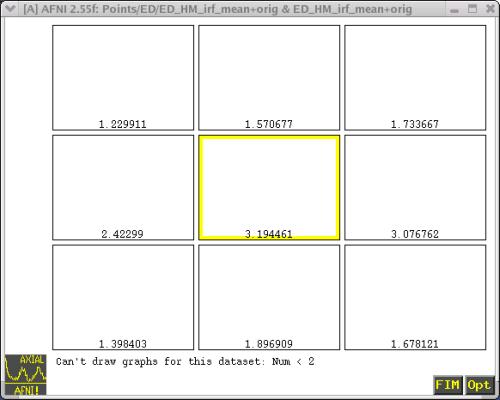 The mean IRF datasets for each condition (i.e., "Human Movies", "Tool
Movies", "Human Points", and "Tool Points") can be found in each subject's
directory. For example:
cd Points/ED/
ED_HM_irf_mean+orig.HEAD ED_HM_irf_mean+orig.BRIK
ED_HP_irf_mean+orig.HEAD ED_HP_irf_mean+orig.BRIK
ED_TM_irf_mean+orig.HEAD ED_TM_irf_mean+orig.BRIK
ED_TP_irf_mean+orig.HEAD ED_TP_irf_mean+orig.BRIK
----------------------------------------------------------------------------
----------------------------------------------------------------------------
K. Use AFNI 'adwarp' to resample functional datasets to same grid as our
Talairached anatomical datasets.
-------------------------------
COMMAND: adwarp
This program resamples a 'data parent' dataset to the grid defined by an
'anat parent' parent dataset. In other words, 'adwarp' can take a
functional dataset and resample it to the grid of the anatomical dataset.
Usage: 3dbucket [options]
(see also '3dbucket -help)
------------------------------------
* EXAMPLE of 3dbucket
In this example, we will be using 'adwarp' to resample the mean IRF
datasets for each subject to the same grid as their Talairached anatomical
dataset. The command from our script is shown below:
foreach cond (TM HM TP HP)
adwarp -apar {$subj}spgr+tlrc \
-dpar {$subj}_{$cond}_irf_mean+orig \
end
The result of 'adwarp' will be Talairach transformed IRF datasets. These
datasets can be found in each subject's directory. For instance:
cd Points/ED/
ED_HM_irf_mean+tlrc.HEAD ED_HM_irf_mean+tlrc.BRIK
ED_HP_irf_mean+tlrc.HEAD ED_HP_irf_mean+tlrc.BRIK
ED_TM_irf_mean+tlrc.HEAD ED_TM_irf_mean+tlrc.BRIK
ED_TP_irf_mean+tlrc.HEAD ED_TP_irf_mean+tlrc.BRIK
Note that the "view" for these datasets has changed from "orig" to "tlrc".
These datasets will be incorporated into our ANOVA.
YOU HAVE REACHED THE END OF SCRIPT 1.
THE NEXT STEP IS RUNNING THE ANOVA -- Go back to the main page of how-to 05 and
refer to "AFNI how-to:Part II" and the script "@ht05_script2".
The mean IRF datasets for each condition (i.e., "Human Movies", "Tool
Movies", "Human Points", and "Tool Points") can be found in each subject's
directory. For example:
cd Points/ED/
ED_HM_irf_mean+orig.HEAD ED_HM_irf_mean+orig.BRIK
ED_HP_irf_mean+orig.HEAD ED_HP_irf_mean+orig.BRIK
ED_TM_irf_mean+orig.HEAD ED_TM_irf_mean+orig.BRIK
ED_TP_irf_mean+orig.HEAD ED_TP_irf_mean+orig.BRIK
----------------------------------------------------------------------------
----------------------------------------------------------------------------
K. Use AFNI 'adwarp' to resample functional datasets to same grid as our
Talairached anatomical datasets.
-------------------------------
COMMAND: adwarp
This program resamples a 'data parent' dataset to the grid defined by an
'anat parent' parent dataset. In other words, 'adwarp' can take a
functional dataset and resample it to the grid of the anatomical dataset.
Usage: 3dbucket [options]
(see also '3dbucket -help)
------------------------------------
* EXAMPLE of 3dbucket
In this example, we will be using 'adwarp' to resample the mean IRF
datasets for each subject to the same grid as their Talairached anatomical
dataset. The command from our script is shown below:
foreach cond (TM HM TP HP)
adwarp -apar {$subj}spgr+tlrc \
-dpar {$subj}_{$cond}_irf_mean+orig \
end
The result of 'adwarp' will be Talairach transformed IRF datasets. These
datasets can be found in each subject's directory. For instance:
cd Points/ED/
ED_HM_irf_mean+tlrc.HEAD ED_HM_irf_mean+tlrc.BRIK
ED_HP_irf_mean+tlrc.HEAD ED_HP_irf_mean+tlrc.BRIK
ED_TM_irf_mean+tlrc.HEAD ED_TM_irf_mean+tlrc.BRIK
ED_TP_irf_mean+tlrc.HEAD ED_TP_irf_mean+tlrc.BRIK
Note that the "view" for these datasets has changed from "orig" to "tlrc".
These datasets will be incorporated into our ANOVA.
YOU HAVE REACHED THE END OF SCRIPT 1.
THE NEXT STEP IS RUNNING THE ANOVA -- Go back to the main page of how-to 05 and
refer to "AFNI how-to:Part II" and the script "@ht05_script2".