HOW-TO #5
A Cornucopia of Statistical Goodies:
Understanding t-tests, ANOVA, and Calculating Percent Change
Analysis of variance, or ANOVA, is a statistical procedure commonly used by
researchers from a wide array of disciplines, including psychology and
neuroscience. ANOVAs are often used in the FMRI community to make comparisons
of signal activation across subjects. For this reason, we provide a brief
introduction to ANOVA in this how-to. Be warned, however, that thick volumes
have been written on analysis of variance, and the information provided in this
how-to can in no way duplicate those efforts. This how-to will simply provide a
very general overview of ANOVA (no ugly equations, I promise!). In addition,
there will be a brief discussion regarding independent- versus paired-samples
t-tests. Finally, we will conclude with a discussion on calculating percent
change and why this normalization method is important when running ANOVA.
TABLE OF CONTENTS
-----------------
I. Independent Samples t-test
II. Paired Samples t-test
III. One-way Analysis of variance (ANOVA)
IV. Two-way ANOVA
V. Parameter Normalization - Calculating Percent Change
I. t-test for INDEPENDENT SAMPLES
------------------------------
Instead of going directly into an explanation of ANOVA, it is perhaps more
beneficial to begin with ANOVA's younger sibling, the t-test. Since ANOVA is
based on the principles of t-tests, a review of the t-test will hopefully make
ANOVA more comprehensible.
When exactly should a t-test be used? When making simple, straightforward
comparisons between two independent samples, the independent samples t-test is
usually the statistic of choice. For clarity, we begin with an example that
implements the independent samples t-test.
EXAMPLE of Independent Samples t-test:
-------------------------------------
Suppose a standardized vocabulary test is given to a group of students.
his sample consists of 120 high school seniors, with an equal number of
males and females. In other words, our study consists of two independent
samples: 60 males and 60 females who are high school seniors. We are
curious to know if there are any significant sex differences in performance
on the standardized vocabulary test. What statistical procedure can be used
to best address this question? The Independent samples t-test.
An independent samples t-test is used to compare the means of two different
samples. In this example, our two samples are MALES and FEMALES, which
make up our single independent variable, "sex."
An independent samples t-test is appropriate when there is one independent
variable (IV) with two levels. For instance, a comparison of young and
older adults' performance on a memory test could be examined using an
independent samples t-test. This type of t-test could also be used to
examine if there is significantly less sneezing in patients administered
Allergy Drug A versus other patients who are given a placebo. In general,
if a study consists of two samples that share a variable of interest, and
group membership does not overlap, then a comparison on some dependent
variable can be made between these two groups.
The first thing to do is clearly label our independent and dependent
variables (also known as "factors"). Recall that the independent variable
(IV) is the factor being manipulated by the experimenter, whereas the
dependent variable (DV) is the factor being measured (i.e., the result of
interest). In this case, the IV is 'sex' with two levels: male and female
(Note: 'sex' or 'gender' is sometimes called a quasi-independent variable
because the experimenter cannot assign a sex to each subject. The
subject already comes to the experiment as either male or female). The
dependent variable in this example is 'vocabulary test score'.
A data spreadsheet for this example may look like this:
SEX ID # VOCAB. SCORE (max=100)
--- ---- ----------------------
F 001 85
F 002 96
F 003 72
. . .
. . .
F 060 64
M 001 56
M 002 100
M 003 82
. . .
. . .
M 060 45
The question of interest is whether the mean test score for the females in
our sample will differ significantly from the mean test score of the males
in our sample. To answer this question, an independent samples t-test must
be performed.
The output from the t-test can be presented in a table and a figure,
as shown below:
Descriptive Statistics:
DV IV N Mean SD SE Mean
-- -- --- ---- -- -------
Vocab Males 60 75.6 10.6 1.37
Females 60 76.4 13.9 1.79
Independent Samples t-test:
t-value df p-value
------- -- -------
1.22 118 .224
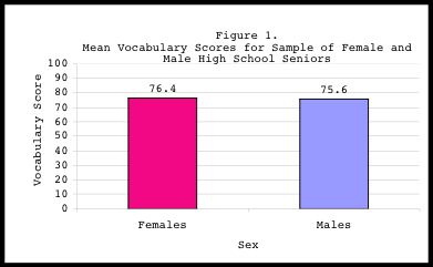 The results suggest that our DV "vocabulary test score" did not differ
significantly between the two levels of our IV "sex." That is, males and
females did not differ significantly in their performance on the vocabulary
test (t=1.22, p>.05). The results are often made clearer if a figure is
drawn. In fact, it is probably good practice to plot out the results to
gain a better understanding of the results, especially when examining main
effects and interactions in ANOVA. As my old stats teacher used to say,
"If in doubt, plot it out."
With a basic understanding of the Independent samples t-test, we can quickly
cover the next topic: Paired Samples t-tests.
II. t-test for PAIRED SAMPLES
------------------------------
The paired samples t-test is usually based on groups of individuals who
experience both conditions of the variable of interest. For instance, one
study might examine the effects of Drug A versus Drug B on a single sample of
100 diabetics. Subjects in this sample would receive Drug A one week, and
Drug B the next. Another study might look at a sample of older adults and their
mean reaction times to two types of stimulus conditions: incongruent color-word
pairs (e.g., the word "blue" printed in red ink) and congruent color-word pairs
(e.g., the word "blue" printed in blue ink). In each of these cases,
participants receive both drug/stimulus conditions.
EXAMPLE of Paired Samples t-test:
--------------------------------
Suppose our group of 120 high-school seniors was given two different
vocabulary quizzes. The question of interest in this case is whether test
performance varies significantly, depending on the quiz given. In other
words, do participants perform similarly or significantly different between
the two quizzes? In this example, our independent variables or factors of
interest are Quiz 1 and Quiz 2. Our dependent measure will be the score or
performance for each quiz. All 120 subjects will be administered these two
quizzes, and the paired samples t-test will be used to determine if
participants' test scores differ significantly between the two quizzes.
A data spreadsheet for this example may look like this:
SUBJECT ID # QUIZ 1 SCORE QUIZ 2 SCORE
------------ ------------ ------------
001 66 72
002 71 80
003 80 83
. . .
. . .
118 64 70
119 56 66
120 32 30
The question of interest is whether the mean score for Quiz 1 differs
significantly from the mean score for Quiz 2. To answer this question, a
paired samples t-test must be performed.
The output from the t-test may look something like this:
Descriptive Statistics:
Variables N Correlation p Mean SD SE
--------- --- ----------- --- ----- --- ---
Quiz 1 120 .673 .000 69.2 8.4 0.77
Quiz 2 79.0 6.2 0.57
Paired Samples t-test:
t-value df p-value
------- -- -------
-2.87 119 .005
The results suggest that our DV "vocabulary test score" did not differ
significantly between the two levels of our IV "sex." That is, males and
females did not differ significantly in their performance on the vocabulary
test (t=1.22, p>.05). The results are often made clearer if a figure is
drawn. In fact, it is probably good practice to plot out the results to
gain a better understanding of the results, especially when examining main
effects and interactions in ANOVA. As my old stats teacher used to say,
"If in doubt, plot it out."
With a basic understanding of the Independent samples t-test, we can quickly
cover the next topic: Paired Samples t-tests.
II. t-test for PAIRED SAMPLES
------------------------------
The paired samples t-test is usually based on groups of individuals who
experience both conditions of the variable of interest. For instance, one
study might examine the effects of Drug A versus Drug B on a single sample of
100 diabetics. Subjects in this sample would receive Drug A one week, and
Drug B the next. Another study might look at a sample of older adults and their
mean reaction times to two types of stimulus conditions: incongruent color-word
pairs (e.g., the word "blue" printed in red ink) and congruent color-word pairs
(e.g., the word "blue" printed in blue ink). In each of these cases,
participants receive both drug/stimulus conditions.
EXAMPLE of Paired Samples t-test:
--------------------------------
Suppose our group of 120 high-school seniors was given two different
vocabulary quizzes. The question of interest in this case is whether test
performance varies significantly, depending on the quiz given. In other
words, do participants perform similarly or significantly different between
the two quizzes? In this example, our independent variables or factors of
interest are Quiz 1 and Quiz 2. Our dependent measure will be the score or
performance for each quiz. All 120 subjects will be administered these two
quizzes, and the paired samples t-test will be used to determine if
participants' test scores differ significantly between the two quizzes.
A data spreadsheet for this example may look like this:
SUBJECT ID # QUIZ 1 SCORE QUIZ 2 SCORE
------------ ------------ ------------
001 66 72
002 71 80
003 80 83
. . .
. . .
118 64 70
119 56 66
120 32 30
The question of interest is whether the mean score for Quiz 1 differs
significantly from the mean score for Quiz 2. To answer this question, a
paired samples t-test must be performed.
The output from the t-test may look something like this:
Descriptive Statistics:
Variables N Correlation p Mean SD SE
--------- --- ----------- --- ----- --- ---
Quiz 1 120 .673 .000 69.2 8.4 0.77
Quiz 2 79.0 6.2 0.57
Paired Samples t-test:
t-value df p-value
------- -- -------
-2.87 119 .005
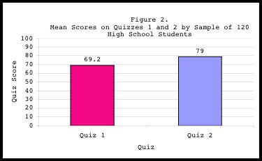 The paired-sample analysis indicates that for the 120 participants, the
mean score on the second quiz (M=79.0) was significantly higher (p=.005)
than the mean score on the first quiz (M=69.2). Figure 2 clearly shows
that on average, subjects performed higher on Quiz 2 than on Quiz 1. These
results also indicate that a significant positive correlation exists
between these two variables (r=.673, p<.001), suggesting that students who
score high on one of the quizzes tend to score high on the other.
Likewise, students who score low on one quiz also tend to also score low on
the other.
With the basics of t-tests covered, it is now time to proceed to the ever-
elusive Analysis of Variance (ANOVA).
III. ONE-WAY ANALYSIS OF VARIANCE (ANOVA)
------------------------------------
Analysis of variance (ANOVA) is a statistical procedure used for comparing
sample means. The results of the ANOVA can be used to infer that the means of
the corresponding population distributions also differ. Whereas t-tests compare
only two sample distributions, ANOVA is capable of comparing many.
As a study becomes increasingly complicated, more complex statistical measures
must also be used. In the examples above, a comparison of two means was made,
making the t-test a sufficient statistical tool. However, if a study involves
one independent variable with more than just two levels or means, then a one-way
ANOVA will be an appropriate alternative to the t-test.
EXAMPLE of One-Way ANOVA:
------------------------
Suppose we were conducting a study on high school students' opinions
regarding the cafeteria food, and asked a sample of 100 students to rate
the quality of the cafeteria food on a scale of 1 to 10 (1 = "I'd rather
eat dog food", 10 = "Pretty darn good"). Our main objective for this study
is to determine if there is a difference in the rating of cafeteria food,
depending on a student's grade level. As such, our independent variable or
factor would be GRADE LEVEL, consisting of 4 levels: 9th, 10th, 11th, and
12th grades. Our dependent variable would be CAFETERIA FOOD RATING.
One may ask, could multiple independent samples t-tests be done to examine
the differences in cafeteria food ratings between class grades? That is,
couldn't we just do several independent t-tests rather than a single one-
way ANOVA? For example:
Comparison of cafeteria food ratings for:
9th vs. 10th grade
9th vs. 11th grade
9th vs. 12th grade
10th vs. 11th grade
10th vs. 12th grade
11th vs. 12th grade
The answer is both 'yes' and 'no'. In theory, it IS possible to do
multiple t-tests instead of a single ANOVA, but in practice, it may not be
the smartest strategy. ANOVA offers numerous advantages that t-tests
cannot provide. Specifically, ANOVA is a very robust measure that allows
the user to avoid the dreaded "inflated alpha" that may arise from
conducting several t-tests.
Side Note - Watch out for Inflated Alpha!
-----------------------------------------
What exactly is inflated alpha? Suppose we run several t-tests and set our
p-value to less than .05. A p<.05 tells us that the probability of getting
statistically significant results simply by chance is less than 5%.
However - and this is a big "however" - conducting multiple t-tests may
lead to what is known as an "inflated alpha." This is when the null
hypothesis is erroneously rejected. In this example, the null hypothesis
is that no significant differences exist in food rating between class
grades. Erroneous rejection of the null hypothesis is also known as a
Type 1 error or a false positive.
As more independent t-tests are done, the probability of getting a Type 1
error increases. In our example, there are only six possible t-tests that
can be done, so alpha inflation is not a major problem. However, suppose
one was testing the effectiveness of ten different types of allergy drugs.
The number of t-test comparisons that can be done in this sample would be
45! See below:
Drug 1 vs. Drug 2 Drug 2 vs. Drug 9 Drug 5 vs. Drug 6
Drug 1 vs. Drug 3 Drug 2 vs. Drug 10 Drug 5 vs. Drug 7
Drug 1 vs. Drug 4 Drug 3 vs. Drug 4 Drug 5 vs. Drug 8
Drug 1 vs. Drug 5 Drug 3 vs. Drug 5 Drug 5 vs. Drug 9
Drug 1 vs. Drug 6 Drug 3 vs. Drug 6 Drug 5 vs. Drug 10
Drug 1 vs. Drug 7 Drug 3 vs. Drug 7 Drug 6 vs. Drug 7
Drug 1 vs. Drug 8 Drug 3 vs. Drug 8 Drug 6 vs. Drug 8
Drug 1 vs. Drug 9 Drug 3 vs. Drug 9 Drug 6 vs. Drug 9
Drug 1 vs. Drug 10 Drug 3 vs. Drug 10 Drug 6 vs. Drug 10
Drug 2 vs. Drug 3 Drug 4 vs. Drug 5 Drug 7 vs. Drug 8
Drug 2 vs. Drug 4 Drug 4 vs. Drug 6 Drug 7 vs. Drug 9
Drug 2 vs. Drug 5 Drug 4 vs. Drug 7 Drug 7 vs. Drug 10
Drug 2 vs. Drug 6 Drug 4 vs. Drug 8 Drug 8 vs. Drug 9
Drug 2 vs. Drug 7 Drug 4 vs. Drug 9 Drug 8 vs. Drug 10
Drug 2 vs. Drug 8 Drug 4 vs. Drug 10 Drug 9 vs. Drug 10
The above example illustrates a study that might be in danger of alpha
inflation if multiple t-tests were conducted rather than a single one-way
ANOVA. Of course, if one insists on running multiple t-tests, then the
best way to avoid alpha inflation is to adjust the p-value to a more
conservative level (e.g., A p-value of .05 divided by 45 comparisons
results in a p=.001). Even with this correction, running this many t-tests
is a bit cumbersome (and will inevitably send any editor reading the
Results section of your manuscript into a tizzy). It is probably better to
run the ANOVA, determine if any differences exist in the first place, and
then run specific t-tests to determine where those differences lie.
Enough about Inflated Alpha. Back to our example...
A spreadsheet for our study on high school students' rating of
cafeteria food might look like this:
GRADE ID # FOOD RATING (range 1-10)
----- ---- -----------
9 001 10
9 002 5
. . .
. . .
10 101 8
10 102 3
. . .
. . .
11 201 5
11 202 9
. . .
. . .
12 301 7
12 302 9
. . .
. . .
A one-way ANOVA can be conducted on this data, with "cafeteria food rating"
as our dependent measure, and "grade" (with four levels) as our independent
measure. The mean food ratings for each class grade are shown in the output
and figure below:
Descriptive Statistics:
IV levels N Mean Food Rating SD SE Min Max
--------- --- ---------------- -- -- --- ---
9th grade 20 8.35 1.53 0.34 6 10
10th grade 24 7.75 2.13 0.44 4 10
11th grade 45 8.04 2.26 0.34 2 10
12th grade 11 6.27 3.32 1.00 2 10
-----------------------------------------------------------------
TOTAL 100 7.84 2.29 0.23 2 10
One-way ANOVA:
DV: Food Rating
Sum Squares df Mean Square F p
----------- -- ----------- --- ---
Between Groups 34.297 3 11.432 2.272 .085
Within Groups 483.143 96 5.033
---------------------------------
TOTAL 517.440 99
The paired-sample analysis indicates that for the 120 participants, the
mean score on the second quiz (M=79.0) was significantly higher (p=.005)
than the mean score on the first quiz (M=69.2). Figure 2 clearly shows
that on average, subjects performed higher on Quiz 2 than on Quiz 1. These
results also indicate that a significant positive correlation exists
between these two variables (r=.673, p<.001), suggesting that students who
score high on one of the quizzes tend to score high on the other.
Likewise, students who score low on one quiz also tend to also score low on
the other.
With the basics of t-tests covered, it is now time to proceed to the ever-
elusive Analysis of Variance (ANOVA).
III. ONE-WAY ANALYSIS OF VARIANCE (ANOVA)
------------------------------------
Analysis of variance (ANOVA) is a statistical procedure used for comparing
sample means. The results of the ANOVA can be used to infer that the means of
the corresponding population distributions also differ. Whereas t-tests compare
only two sample distributions, ANOVA is capable of comparing many.
As a study becomes increasingly complicated, more complex statistical measures
must also be used. In the examples above, a comparison of two means was made,
making the t-test a sufficient statistical tool. However, if a study involves
one independent variable with more than just two levels or means, then a one-way
ANOVA will be an appropriate alternative to the t-test.
EXAMPLE of One-Way ANOVA:
------------------------
Suppose we were conducting a study on high school students' opinions
regarding the cafeteria food, and asked a sample of 100 students to rate
the quality of the cafeteria food on a scale of 1 to 10 (1 = "I'd rather
eat dog food", 10 = "Pretty darn good"). Our main objective for this study
is to determine if there is a difference in the rating of cafeteria food,
depending on a student's grade level. As such, our independent variable or
factor would be GRADE LEVEL, consisting of 4 levels: 9th, 10th, 11th, and
12th grades. Our dependent variable would be CAFETERIA FOOD RATING.
One may ask, could multiple independent samples t-tests be done to examine
the differences in cafeteria food ratings between class grades? That is,
couldn't we just do several independent t-tests rather than a single one-
way ANOVA? For example:
Comparison of cafeteria food ratings for:
9th vs. 10th grade
9th vs. 11th grade
9th vs. 12th grade
10th vs. 11th grade
10th vs. 12th grade
11th vs. 12th grade
The answer is both 'yes' and 'no'. In theory, it IS possible to do
multiple t-tests instead of a single ANOVA, but in practice, it may not be
the smartest strategy. ANOVA offers numerous advantages that t-tests
cannot provide. Specifically, ANOVA is a very robust measure that allows
the user to avoid the dreaded "inflated alpha" that may arise from
conducting several t-tests.
Side Note - Watch out for Inflated Alpha!
-----------------------------------------
What exactly is inflated alpha? Suppose we run several t-tests and set our
p-value to less than .05. A p<.05 tells us that the probability of getting
statistically significant results simply by chance is less than 5%.
However - and this is a big "however" - conducting multiple t-tests may
lead to what is known as an "inflated alpha." This is when the null
hypothesis is erroneously rejected. In this example, the null hypothesis
is that no significant differences exist in food rating between class
grades. Erroneous rejection of the null hypothesis is also known as a
Type 1 error or a false positive.
As more independent t-tests are done, the probability of getting a Type 1
error increases. In our example, there are only six possible t-tests that
can be done, so alpha inflation is not a major problem. However, suppose
one was testing the effectiveness of ten different types of allergy drugs.
The number of t-test comparisons that can be done in this sample would be
45! See below:
Drug 1 vs. Drug 2 Drug 2 vs. Drug 9 Drug 5 vs. Drug 6
Drug 1 vs. Drug 3 Drug 2 vs. Drug 10 Drug 5 vs. Drug 7
Drug 1 vs. Drug 4 Drug 3 vs. Drug 4 Drug 5 vs. Drug 8
Drug 1 vs. Drug 5 Drug 3 vs. Drug 5 Drug 5 vs. Drug 9
Drug 1 vs. Drug 6 Drug 3 vs. Drug 6 Drug 5 vs. Drug 10
Drug 1 vs. Drug 7 Drug 3 vs. Drug 7 Drug 6 vs. Drug 7
Drug 1 vs. Drug 8 Drug 3 vs. Drug 8 Drug 6 vs. Drug 8
Drug 1 vs. Drug 9 Drug 3 vs. Drug 9 Drug 6 vs. Drug 9
Drug 1 vs. Drug 10 Drug 3 vs. Drug 10 Drug 6 vs. Drug 10
Drug 2 vs. Drug 3 Drug 4 vs. Drug 5 Drug 7 vs. Drug 8
Drug 2 vs. Drug 4 Drug 4 vs. Drug 6 Drug 7 vs. Drug 9
Drug 2 vs. Drug 5 Drug 4 vs. Drug 7 Drug 7 vs. Drug 10
Drug 2 vs. Drug 6 Drug 4 vs. Drug 8 Drug 8 vs. Drug 9
Drug 2 vs. Drug 7 Drug 4 vs. Drug 9 Drug 8 vs. Drug 10
Drug 2 vs. Drug 8 Drug 4 vs. Drug 10 Drug 9 vs. Drug 10
The above example illustrates a study that might be in danger of alpha
inflation if multiple t-tests were conducted rather than a single one-way
ANOVA. Of course, if one insists on running multiple t-tests, then the
best way to avoid alpha inflation is to adjust the p-value to a more
conservative level (e.g., A p-value of .05 divided by 45 comparisons
results in a p=.001). Even with this correction, running this many t-tests
is a bit cumbersome (and will inevitably send any editor reading the
Results section of your manuscript into a tizzy). It is probably better to
run the ANOVA, determine if any differences exist in the first place, and
then run specific t-tests to determine where those differences lie.
Enough about Inflated Alpha. Back to our example...
A spreadsheet for our study on high school students' rating of
cafeteria food might look like this:
GRADE ID # FOOD RATING (range 1-10)
----- ---- -----------
9 001 10
9 002 5
. . .
. . .
10 101 8
10 102 3
. . .
. . .
11 201 5
11 202 9
. . .
. . .
12 301 7
12 302 9
. . .
. . .
A one-way ANOVA can be conducted on this data, with "cafeteria food rating"
as our dependent measure, and "grade" (with four levels) as our independent
measure. The mean food ratings for each class grade are shown in the output
and figure below:
Descriptive Statistics:
IV levels N Mean Food Rating SD SE Min Max
--------- --- ---------------- -- -- --- ---
9th grade 20 8.35 1.53 0.34 6 10
10th grade 24 7.75 2.13 0.44 4 10
11th grade 45 8.04 2.26 0.34 2 10
12th grade 11 6.27 3.32 1.00 2 10
-----------------------------------------------------------------
TOTAL 100 7.84 2.29 0.23 2 10
One-way ANOVA:
DV: Food Rating
Sum Squares df Mean Square F p
----------- -- ----------- --- ---
Between Groups 34.297 3 11.432 2.272 .085
Within Groups 483.143 96 5.033
---------------------------------
TOTAL 517.440 99
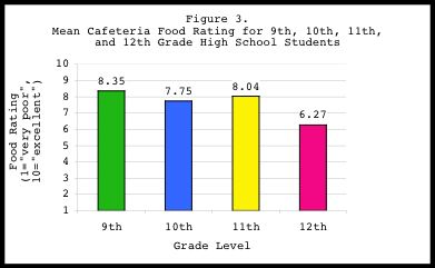 The F-score and p-value of a one-way ANOVA will indicate whether the main
effect of the independent variable "class grade" was significant. In other
words, a significant F-statistic would tell us that class grade had a
significant effect on cafeteria food rating. In this example, our p-value
of .085 suggests that a marginally significant difference exists within
comparisons of food ratings among our four grade levels.
Although the ANOVA results tell us that grade-related differences exist in
cafeteria food ratings, it does not tell us 'where' those differences lie.
Is it between 9th and 12th graders? 10th and 11th? Additional post-hoc
tests must be done to address this issue. The results of the post-hoc
tests are shown below:
Post Hoc Tests (note: these are independent t-tests):
Grade(I) Grade(J) Mean (I-J) SE p-value
------- ------- ---------- ---- -------
9th vs. 10th .60 .679 .379
9th vs. 11th .31 .603 .613
9th vs. 12th 2.08* .842 .015
10th vs. 11th -.29 .567 .605
10th vs. 12th 1.48 .817 .074
11th vs. 12th 1.77* .755 .021
The asterisks (*) indicate there are two pairs of groups whose means differ
significantly (p<.05) from each other. 12th graders seem to dislike the
cafeteria food significantly more than both 9th and 11th graders (p=.015
and .021 respectively). Seniors also dislike the cafeteria food marginally
more than 10th graders (p=.074)
Why did the overall ANOVA show only a marginally significant difference
(p=.085), while the pair-wise comparisons yielded two differences (i.e.,
9th vs. 12th and 11th vs. 12th) that were strongly significant? This is
because the overall ANOVA compares all values simultaneously, thus
weakening statistical power. The post-hoc tests are simply a series of
independent t-tests.
IV. TWO-WAY ANALYSIS OF VARIANCE
----------------------------
A two-way (or two-factor) ANOVA is a procedure that designates a single
dependent variable and utilizes exactly two independent variables to gain an
understanding of how the IV's influence the DV.
WARNING:
When conducting ANOVA, it is relatively easy to get certain software packages
(like SPSS, SAS, SPM, AFNI, etc.) to conduct a two-way, three-way, even four-
or five-way analysis of variance. The programs may do all the arithmetic, which
results in impressive-looking output, but it is up to the user to properly
interpret those results. The ease of calculating analysis of variance on the
computer often masks the fact that a successful study requires many hours of
careful planning. In addition, a one-way ANOVA is fairly straightforward and
easy to interpret, but a two-way ANOVA requires some training and frequently
involves a thorough examination of tables and figures before interpretation is
clear. Understanding a three-way ANOVA usually requires an experienced
researcher, and interpretation of a four-way ANOVA is often nightmarish in
nature, even for the most skilled researcher.
EXAMPLE of Two-Way ANOVA:
-------------------------
Suppose we were interested in determining if performance on a math test
would differ between males and females given chocolate, vanilla, or
strawberry ice cream before taking the test (yes, this is a silly example
but just go with it). In this example, we have two independent variables
and one dependent variable (side note: more than one DV would require a
MANOVA). As such, the design of our experiment is set up in the following
manner:
IV1: SEX (Females, Males)
IV2: FLAVOR (Chocolate, Vanilla, Strawberry)
DV: MATH TEST SCORE
In this example, we have a 2 x 3 between-subjects design. The design is
labeled "between-subjects" because participants fall under only one level
of each independent variable. For instance, subjects are either male or
female, and they are either given chocolate, vanilla, or strawberry ice
cream. There is no overlap of our subject groups. As such, our data
spreadsheet might look like this:
SEX FLAVOR ID# MATH TEST SCORE
--- ------ --- ---------------
F chocolate 001 104
F chocolate 002 89
. . . .
. . . .
F vanilla 101 98
F vanilla 102 100
. . . .
. . . .
F strawberry 201 80
F strawberry 202 77
. . . .
. . . .
M chocolate 301 98
M chocolate 302 106
. . . .
. . . .
M vanilla 401 78
M vanilla 402 70
. . . .
. . . .
M strawberry 501 88
M strawberry 502 102
. . . .
. . . .
By running a two-way ANOVA on the data, we hope to answer the following
questions: First, is there a main effect of SEX? That is, do males and
females differ significantly on their performance on the math test?
Second, is there a main effect of FLAVOR, where a significant difference
in math performance can be found between chocolate, vanilla, and strawberry
ice cream eaters? Finally, is there a significant SEX by FLAVOR
interaction? That is, how do sex and flavor interact in their effect on
math test performance? Can any sex differences in math performance be found
between the three different ice cream flavors?
The output of our two-way ANOVA is shown below:
Descriptive Statistics:
DV = Math Score
Flavor Sex Mean Score Std. Dev N
------ --- ---------- -------- --
Chocolate Female 103.95 18.14 20
Male 106.85 13.01 13
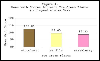
TOTAL 105.09 16.15 33
Vanilla Female 100.00 12.31 26
Male 98.46 11.82 13
TOTAL 99.49 12.01 33
Strawberry Female 102.83 10.68 18
Male 90.73 21.23 15
TOTAL 97.33 17.18 33
-----------------------------------------------------------
TOTAL Female 102.03 13.90 64
Male 98.29 17.20 41
TOTAL 100.57 15.30 105
Two-way ANOVA:
Source Sum Squares df Mean Square F p
------ ----------- --- ------------ --- ---
Corrected 2350.41 5 470.08 2.12 .070
Model
Intercept 996892.70 1 996892.70 4487.39 .000
FLAVOR 1262.73 2 631.36 2.84 .063
SEX 316.56 1 316.56 1.43 .235
FLAVOR * SEX 960.44 2 480.22 2.16 .121
Error 21993.31 99 222.16
Total 1086378.00 105
Corrected Err. 24343.71 104
Main Effect of FLAVOR:
---------------------
The above results indicate that our main effect of FLAVOR was
marginally significant (F(2,99)=2.84, p=.063), suggesting that math
scores differed somewhat between the three flavor groups. To clarify
this main effect further, it is always helpful to plot out the
results. Figure 4 shows that collapsed across SEX, chocolate tasters
scored marginally higher on the math test than strawberry and vanilla
tasters. Vanilla and strawberry tasters did not seem to differ on
their math test performance.
The F-score and p-value of a one-way ANOVA will indicate whether the main
effect of the independent variable "class grade" was significant. In other
words, a significant F-statistic would tell us that class grade had a
significant effect on cafeteria food rating. In this example, our p-value
of .085 suggests that a marginally significant difference exists within
comparisons of food ratings among our four grade levels.
Although the ANOVA results tell us that grade-related differences exist in
cafeteria food ratings, it does not tell us 'where' those differences lie.
Is it between 9th and 12th graders? 10th and 11th? Additional post-hoc
tests must be done to address this issue. The results of the post-hoc
tests are shown below:
Post Hoc Tests (note: these are independent t-tests):
Grade(I) Grade(J) Mean (I-J) SE p-value
------- ------- ---------- ---- -------
9th vs. 10th .60 .679 .379
9th vs. 11th .31 .603 .613
9th vs. 12th 2.08* .842 .015
10th vs. 11th -.29 .567 .605
10th vs. 12th 1.48 .817 .074
11th vs. 12th 1.77* .755 .021
The asterisks (*) indicate there are two pairs of groups whose means differ
significantly (p<.05) from each other. 12th graders seem to dislike the
cafeteria food significantly more than both 9th and 11th graders (p=.015
and .021 respectively). Seniors also dislike the cafeteria food marginally
more than 10th graders (p=.074)
Why did the overall ANOVA show only a marginally significant difference
(p=.085), while the pair-wise comparisons yielded two differences (i.e.,
9th vs. 12th and 11th vs. 12th) that were strongly significant? This is
because the overall ANOVA compares all values simultaneously, thus
weakening statistical power. The post-hoc tests are simply a series of
independent t-tests.
IV. TWO-WAY ANALYSIS OF VARIANCE
----------------------------
A two-way (or two-factor) ANOVA is a procedure that designates a single
dependent variable and utilizes exactly two independent variables to gain an
understanding of how the IV's influence the DV.
WARNING:
When conducting ANOVA, it is relatively easy to get certain software packages
(like SPSS, SAS, SPM, AFNI, etc.) to conduct a two-way, three-way, even four-
or five-way analysis of variance. The programs may do all the arithmetic, which
results in impressive-looking output, but it is up to the user to properly
interpret those results. The ease of calculating analysis of variance on the
computer often masks the fact that a successful study requires many hours of
careful planning. In addition, a one-way ANOVA is fairly straightforward and
easy to interpret, but a two-way ANOVA requires some training and frequently
involves a thorough examination of tables and figures before interpretation is
clear. Understanding a three-way ANOVA usually requires an experienced
researcher, and interpretation of a four-way ANOVA is often nightmarish in
nature, even for the most skilled researcher.
EXAMPLE of Two-Way ANOVA:
-------------------------
Suppose we were interested in determining if performance on a math test
would differ between males and females given chocolate, vanilla, or
strawberry ice cream before taking the test (yes, this is a silly example
but just go with it). In this example, we have two independent variables
and one dependent variable (side note: more than one DV would require a
MANOVA). As such, the design of our experiment is set up in the following
manner:
IV1: SEX (Females, Males)
IV2: FLAVOR (Chocolate, Vanilla, Strawberry)
DV: MATH TEST SCORE
In this example, we have a 2 x 3 between-subjects design. The design is
labeled "between-subjects" because participants fall under only one level
of each independent variable. For instance, subjects are either male or
female, and they are either given chocolate, vanilla, or strawberry ice
cream. There is no overlap of our subject groups. As such, our data
spreadsheet might look like this:
SEX FLAVOR ID# MATH TEST SCORE
--- ------ --- ---------------
F chocolate 001 104
F chocolate 002 89
. . . .
. . . .
F vanilla 101 98
F vanilla 102 100
. . . .
. . . .
F strawberry 201 80
F strawberry 202 77
. . . .
. . . .
M chocolate 301 98
M chocolate 302 106
. . . .
. . . .
M vanilla 401 78
M vanilla 402 70
. . . .
. . . .
M strawberry 501 88
M strawberry 502 102
. . . .
. . . .
By running a two-way ANOVA on the data, we hope to answer the following
questions: First, is there a main effect of SEX? That is, do males and
females differ significantly on their performance on the math test?
Second, is there a main effect of FLAVOR, where a significant difference
in math performance can be found between chocolate, vanilla, and strawberry
ice cream eaters? Finally, is there a significant SEX by FLAVOR
interaction? That is, how do sex and flavor interact in their effect on
math test performance? Can any sex differences in math performance be found
between the three different ice cream flavors?
The output of our two-way ANOVA is shown below:
Descriptive Statistics:
DV = Math Score
Flavor Sex Mean Score Std. Dev N
------ --- ---------- -------- --
Chocolate Female 103.95 18.14 20
Male 106.85 13.01 13
TOTAL 105.09 16.15 33
Vanilla Female 100.00 12.31 26
Male 98.46 11.82 13
TOTAL 99.49 12.01 33
Strawberry Female 102.83 10.68 18
Male 90.73 21.23 15
TOTAL 97.33 17.18 33
-----------------------------------------------------------
TOTAL Female 102.03 13.90 64
Male 98.29 17.20 41
TOTAL 100.57 15.30 105
Two-way ANOVA:
Source Sum Squares df Mean Square F p
------ ----------- --- ------------ --- ---
Corrected 2350.41 5 470.08 2.12 .070
Model
Intercept 996892.70 1 996892.70 4487.39 .000
FLAVOR 1262.73 2 631.36 2.84 .063
SEX 316.56 1 316.56 1.43 .235
FLAVOR * SEX 960.44 2 480.22 2.16 .121
Error 21993.31 99 222.16
Total 1086378.00 105
Corrected Err. 24343.71 104
Main Effect of FLAVOR:
---------------------
The above results indicate that our main effect of FLAVOR was
marginally significant (F(2,99)=2.84, p=.063), suggesting that math
scores differed somewhat between the three flavor groups. To clarify
this main effect further, it is always helpful to plot out the
results. Figure 4 shows that collapsed across SEX, chocolate tasters
scored marginally higher on the math test than strawberry and vanilla
tasters. Vanilla and strawberry tasters did not seem to differ on
their math test performance.
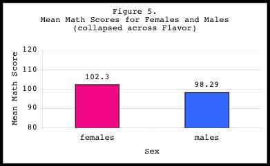
 Main Effect of SEX:
------------------
Our main effect of SEX was not statistically significant
(F(1,99)=1.43, p=.235), indicating no sex-related differences in math
test performance. Again,this result can be seen clearly by collapsing
across FLAVOR, and plotting the mean math scores for males and females
(see Figure 5):
Main Effect of SEX:
------------------
Our main effect of SEX was not statistically significant
(F(1,99)=1.43, p=.235), indicating no sex-related differences in math
test performance. Again,this result can be seen clearly by collapsing
across FLAVOR, and plotting the mean math scores for males and females
(see Figure 5):
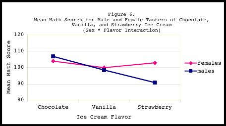
 SEX by FLAVOR Interaction:
-------------------------
Finally, there was no significant SEX by FLAVOR interaction
(F(2,99)=2.16, p=.121). By plotting out the results (see Figure 6),
we clearly see that male and female chocolate tasters performed
virtually identically on the math test. The same result can be seen
between male and female vanilla tasters. However, amongst the
strawberry tasters, we see a pattern (although not statistically
significant) of females performing slightly higher on the math test
than males.
SEX by FLAVOR Interaction:
-------------------------
Finally, there was no significant SEX by FLAVOR interaction
(F(2,99)=2.16, p=.121). By plotting out the results (see Figure 6),
we clearly see that male and female chocolate tasters performed
virtually identically on the math test. The same result can be seen
between male and female vanilla tasters. However, amongst the
strawberry tasters, we see a pattern (although not statistically
significant) of females performing slightly higher on the math test
than males.
 As this example illustrates, it is always a good idea to plot out the
results. A schematic view of the data makes it much easier to decipher
where the significant main effects and interactions may lie. Even if the
results are not statistically significant, a plot will show the pattern of
results, which can be just as informative as the statistical findings.
V. PARAMETER NORMALIZATION - Calculating Percent Change
----------------------------------------------------
Although this section may seem to deviate a bit from the previous sections on
t-tests and ANOVAs, the discussion of calculating percent change is actually
quite relevant to statistical testing. Primarily, the calculation of percent
signal change is a type of normalization of the data, which is necessary when
comparing groups whose baselines differ. When making comparisons across
subjects or groups of subjects, normalization of the data becomes an important
issue. If certain parameters of interest are not normalized before group
comparisons are made, then the results may be misleading, suggesting there are
differences between groups when in fact there are not. To fully understand this
issue, an example is in order:
EXAMPLE of Percent Change:
-------------------------
Suppose we tested a sample of young adults and a sample of older adults on
a reaction time task. The reaction time task has two conditions: the first
one involves color blocks presented on the computer screen. Each
participant must identify the color the block is painted in as quickly as
possible. The second condition consists of color words (e.g., "BLUE")
printed in an incongruent ink color (e.g., red). The goal is to ignore the
word and name the color ink. This second condition is often referred to as
the "Stroop" task. The Stroop task typically slows down reaction time
because participants must first suppress the urge to read the word, and
instead, name the ink color. As such, the Stroop condition should result
in significantly longer response times than the color blocks condition for
both age groups. Our 2 x 2 mixed factorial design is composed of the
following independent and dependent variables:
IV1-AGE: 1. Young
2. Older
IV2-CONDITION: 1. Color blocks
2. Stroop task
DV - RESPONSE TIME (measured in msec)
In this case, AGE is a between-subjects variable because subjects are
either young or older, but not both. Alternatively, CONDITION is a within
subjects variable because participants are exposed to both the color blocks
and the Stroop task. As such, our design is identified as "mixed" because
there are both between- and within-subject variables in our experiment.
The following hypotheses can be formulated for this experiment:
First, do we expect to find a main effect of AGE? If so, we might
predict that with age, reaction time declines, which results in
significantly slower response times for older adults than young
adults.
Second, do we expect to find a main effect of CONDITION? We predict
that the Stroop condition will result in significantly slower response
times for both age groups than the colored blocks condition. This is
because reading is more automatic than color naming. As such,
subjects must take the time to suppress the reading response in order
to correctly name the ink color.
Finally - and most importantly - do we expect to find a significant
AGE x CONDITION interaction? In other words, do older adults show
more slowing in the Stroop condition relative to the color blocks
condition than do young adults? If so, we might conclude that with
age, not only does response time increase, it also becomes more
difficult to suppress irrelevant information, making the Stroop task
more difficult for older than young adults. One reason for such a
finding may be that the ability to block out irrelevant information
becomes compromised with age.
The output for this study may look something like this:
Descriptive Statistics:
DV = Mean Response time (in milliseconds)
Young Adults Older Adults
------------ -------------
A) Color Blocks 500 ms 1000 ms
B) Stroop Task 550 ms 1100 ms
-------------------------------------------------------
Difference (B-A): 50 ms 100 ms
By examining the absolute differences between the Stroop task and the Color
Blocks, we find a difference of 50 ms for young adults and 100 ms for older
adults. From this finding, one might conclude, "Wow, older adults are
twice as slow as young adults when they are presented with the Stroop task.
It is twice as hard for older adults to deal with the Stroop task, which
involves the simultaneous presentation of two pieces of incongruent
information. This must mean that with age, older adults develop inhibitory
deficits that deter them from suppressing irrelevant information."
However, the interpretation of these results may be inaccurate, because it
is not accounting for the fact that the baselines for young and older
adults are different. If the color blocks condition is our
baseline/neutral condition, we see that on average, young adults respond at
around 500 milliseconds. On the other hand, older adults' baseline is much
slower, at 1000 milliseconds. This finding indicates that in general,
older adults have slower response times than young adults. As such, we
must account for these differences in baseline, by calculating the percent
change in response time between the baseline condition and the Stroop
condition. That is, how much slower is each group in the Stroop condition
relative to their baseline? Is it 5 percent for young and 10 percent for
older adults? Is it 10 percent for young and 12 percent for older?
Converting our absolute response times to percent change will allow us to
answer this question.
One way to calculate the percent change is by using the following
simple equation:
A = Baseline Condition (e.g., color blocks response time)
B = Stimulus Condition (e.g., Stroop task response time)
((B - A)/A) * 100 = percent change
We can apply this formula to each of our age groups:
Young Adults:
((550 - 500)/500) * 100 = 10%
Older Adults:
((1100 - 1000)/1000) * 100 = 10%
When the data are normalized, we realize that there really aren't any age-
related differences in Stroop interference between young and older adults.
For both age groups, the Stroop condition slowed participants by 10%
compared to the baseline condition. Although older adults are slower in
general than young adults, both age groups experience the same amount of
interference from the Stroop condition. Therefore, these results do not
suggest that inhibitory deficits increase with age. As such, the
AGE x CONDITION interaction should not be statistically significant. A
plot of the interaction (Figure 7) verifies this conclusion:
As this example illustrates, it is always a good idea to plot out the
results. A schematic view of the data makes it much easier to decipher
where the significant main effects and interactions may lie. Even if the
results are not statistically significant, a plot will show the pattern of
results, which can be just as informative as the statistical findings.
V. PARAMETER NORMALIZATION - Calculating Percent Change
----------------------------------------------------
Although this section may seem to deviate a bit from the previous sections on
t-tests and ANOVAs, the discussion of calculating percent change is actually
quite relevant to statistical testing. Primarily, the calculation of percent
signal change is a type of normalization of the data, which is necessary when
comparing groups whose baselines differ. When making comparisons across
subjects or groups of subjects, normalization of the data becomes an important
issue. If certain parameters of interest are not normalized before group
comparisons are made, then the results may be misleading, suggesting there are
differences between groups when in fact there are not. To fully understand this
issue, an example is in order:
EXAMPLE of Percent Change:
-------------------------
Suppose we tested a sample of young adults and a sample of older adults on
a reaction time task. The reaction time task has two conditions: the first
one involves color blocks presented on the computer screen. Each
participant must identify the color the block is painted in as quickly as
possible. The second condition consists of color words (e.g., "BLUE")
printed in an incongruent ink color (e.g., red). The goal is to ignore the
word and name the color ink. This second condition is often referred to as
the "Stroop" task. The Stroop task typically slows down reaction time
because participants must first suppress the urge to read the word, and
instead, name the ink color. As such, the Stroop condition should result
in significantly longer response times than the color blocks condition for
both age groups. Our 2 x 2 mixed factorial design is composed of the
following independent and dependent variables:
IV1-AGE: 1. Young
2. Older
IV2-CONDITION: 1. Color blocks
2. Stroop task
DV - RESPONSE TIME (measured in msec)
In this case, AGE is a between-subjects variable because subjects are
either young or older, but not both. Alternatively, CONDITION is a within
subjects variable because participants are exposed to both the color blocks
and the Stroop task. As such, our design is identified as "mixed" because
there are both between- and within-subject variables in our experiment.
The following hypotheses can be formulated for this experiment:
First, do we expect to find a main effect of AGE? If so, we might
predict that with age, reaction time declines, which results in
significantly slower response times for older adults than young
adults.
Second, do we expect to find a main effect of CONDITION? We predict
that the Stroop condition will result in significantly slower response
times for both age groups than the colored blocks condition. This is
because reading is more automatic than color naming. As such,
subjects must take the time to suppress the reading response in order
to correctly name the ink color.
Finally - and most importantly - do we expect to find a significant
AGE x CONDITION interaction? In other words, do older adults show
more slowing in the Stroop condition relative to the color blocks
condition than do young adults? If so, we might conclude that with
age, not only does response time increase, it also becomes more
difficult to suppress irrelevant information, making the Stroop task
more difficult for older than young adults. One reason for such a
finding may be that the ability to block out irrelevant information
becomes compromised with age.
The output for this study may look something like this:
Descriptive Statistics:
DV = Mean Response time (in milliseconds)
Young Adults Older Adults
------------ -------------
A) Color Blocks 500 ms 1000 ms
B) Stroop Task 550 ms 1100 ms
-------------------------------------------------------
Difference (B-A): 50 ms 100 ms
By examining the absolute differences between the Stroop task and the Color
Blocks, we find a difference of 50 ms for young adults and 100 ms for older
adults. From this finding, one might conclude, "Wow, older adults are
twice as slow as young adults when they are presented with the Stroop task.
It is twice as hard for older adults to deal with the Stroop task, which
involves the simultaneous presentation of two pieces of incongruent
information. This must mean that with age, older adults develop inhibitory
deficits that deter them from suppressing irrelevant information."
However, the interpretation of these results may be inaccurate, because it
is not accounting for the fact that the baselines for young and older
adults are different. If the color blocks condition is our
baseline/neutral condition, we see that on average, young adults respond at
around 500 milliseconds. On the other hand, older adults' baseline is much
slower, at 1000 milliseconds. This finding indicates that in general,
older adults have slower response times than young adults. As such, we
must account for these differences in baseline, by calculating the percent
change in response time between the baseline condition and the Stroop
condition. That is, how much slower is each group in the Stroop condition
relative to their baseline? Is it 5 percent for young and 10 percent for
older adults? Is it 10 percent for young and 12 percent for older?
Converting our absolute response times to percent change will allow us to
answer this question.
One way to calculate the percent change is by using the following
simple equation:
A = Baseline Condition (e.g., color blocks response time)
B = Stimulus Condition (e.g., Stroop task response time)
((B - A)/A) * 100 = percent change
We can apply this formula to each of our age groups:
Young Adults:
((550 - 500)/500) * 100 = 10%
Older Adults:
((1100 - 1000)/1000) * 100 = 10%
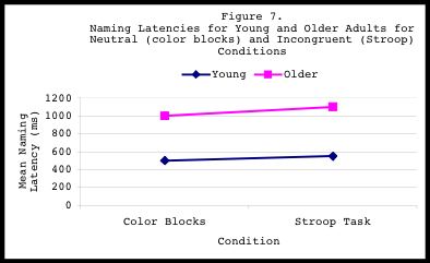
When the data are normalized, we realize that there really aren't any age-
related differences in Stroop interference between young and older adults.
For both age groups, the Stroop condition slowed participants by 10%
compared to the baseline condition. Although older adults are slower in
general than young adults, both age groups experience the same amount of
interference from the Stroop condition. Therefore, these results do not
suggest that inhibitory deficits increase with age. As such, the
AGE x CONDITION interaction should not be statistically significant. A
plot of the interaction (Figure 7) verifies this conclusion:
 FMRI and Calculating Percent Signal Change:
------------------------------------------
The above example showed the importance of normalization of data in a
psychological study. This normalization process is just as important in FMRI
research. When comparing parameters that quantify activation across subjects
(i.e., an ANOVA will be run to examine activation levels across subjects in
response to a stimulus), these parameters should be normalized by calculating
the percent signal change. This is because FMRI signal amplitude varies for
different subjects, runs, scanning sessions, regressors, image reconstruction
software, and modeling strategies. Amplitude measures (i.e., regression
coefficients) can be turned to percent signal change from the baseline. For an
FMRI example of how the percent signal change is calculated using AFNI, see the
AFNI_howto section of this tutorial.
CONCLUSION
----------
The goal of this review was to take some anguish and anxiety out of statistics.
Since we cannot take the statistics out of research, we must conquer and embrace
it. Hopefully, any questions you may have had regarding t-tests, ANOVAs, and
parameter normalization have been adequately answered. Although the examples
shown here come from behavioral research (I'm a psychologist, this is what I
know), the statistics can be applied to FMRI research as well, on a voxel-by-
voxel basis. Although the BOLD signal is a somewhat more complicated dependent
variable than say, a reaction time or a test score, the statistics are the same.
REFERENCES
----------
If this review has whetted your appetite for more statistics, the following
references selected by members of the Scientific and Statistical Computing Core
at the NIMH (http://afni.nimh.nih.gov/sscc) may be of interest to
you. Good luck and happy reading!
Picks by Dr. Cox:
----------------
Bickel, P. J. & Doksum, K. A. (1977). Mathematical Statistics. Holden-Day.
Casella, G. & Berger, R. L. (1990). Statistical Inference. Brooks/Cole.
Picks by Dr. Chen:
-----------------
Kutner, M.H., Nachtschiem, C.J., Wasserman, W., & Neter, J. (1996). Applied
Linear Statistical Models, 4th edition. McGraw-Hill/Irwin.
Neter, J., Wasserman, W., & Kutner, M.H. (1990). Applied Linear Statistical
Models: Regression, Analysis of Variance, and Experimental Designs,
3rd edition. Richard d Irwin Publishing.
Picks by Dr. Christidis:
-----------------------
Howell, D. C. (2003). Fundamental Statistics for the Behavioral Sciences,
5th edition. International Thomson Publishing.
Hays, W. L. (1994). Statistics, 5th edition. International Thomson Publishing.
Helpful website: www.statsoftinc.com/textbook/stanman.html
FMRI and Calculating Percent Signal Change:
------------------------------------------
The above example showed the importance of normalization of data in a
psychological study. This normalization process is just as important in FMRI
research. When comparing parameters that quantify activation across subjects
(i.e., an ANOVA will be run to examine activation levels across subjects in
response to a stimulus), these parameters should be normalized by calculating
the percent signal change. This is because FMRI signal amplitude varies for
different subjects, runs, scanning sessions, regressors, image reconstruction
software, and modeling strategies. Amplitude measures (i.e., regression
coefficients) can be turned to percent signal change from the baseline. For an
FMRI example of how the percent signal change is calculated using AFNI, see the
AFNI_howto section of this tutorial.
CONCLUSION
----------
The goal of this review was to take some anguish and anxiety out of statistics.
Since we cannot take the statistics out of research, we must conquer and embrace
it. Hopefully, any questions you may have had regarding t-tests, ANOVAs, and
parameter normalization have been adequately answered. Although the examples
shown here come from behavioral research (I'm a psychologist, this is what I
know), the statistics can be applied to FMRI research as well, on a voxel-by-
voxel basis. Although the BOLD signal is a somewhat more complicated dependent
variable than say, a reaction time or a test score, the statistics are the same.
REFERENCES
----------
If this review has whetted your appetite for more statistics, the following
references selected by members of the Scientific and Statistical Computing Core
at the NIMH (http://afni.nimh.nih.gov/sscc) may be of interest to
you. Good luck and happy reading!
Picks by Dr. Cox:
----------------
Bickel, P. J. & Doksum, K. A. (1977). Mathematical Statistics. Holden-Day.
Casella, G. & Berger, R. L. (1990). Statistical Inference. Brooks/Cole.
Picks by Dr. Chen:
-----------------
Kutner, M.H., Nachtschiem, C.J., Wasserman, W., & Neter, J. (1996). Applied
Linear Statistical Models, 4th edition. McGraw-Hill/Irwin.
Neter, J., Wasserman, W., & Kutner, M.H. (1990). Applied Linear Statistical
Models: Regression, Analysis of Variance, and Experimental Designs,
3rd edition. Richard d Irwin Publishing.
Picks by Dr. Christidis:
-----------------------
Howell, D. C. (2003). Fundamental Statistics for the Behavioral Sciences,
5th edition. International Thomson Publishing.
Hays, W. L. (1994). Statistics, 5th edition. International Thomson Publishing.
Helpful website: www.statsoftinc.com/textbook/stanman.html