7.2. 1dDW_Grad_o_Mat++: dealing with DW gradients¶

7.2.1. Overview ¶

In diffusion weighted imaging (DWI), magnetic field gradients are applied along various spatial directions to probe relative diffusivity along different orientations. In order to estimate the diffusion tensor (DT), we need to have a recording of what was the directionality of each gradient (g, a vector of unit length), and what was the strength of the extra magnetic field (b, a scalar) was used.

Many different programs and software, starting from the MRI machines themselves, use different notations and methods of reading and writing the gradient direction and strength information. Drat. Therefore, there is some need for manipulating them during the analysis process (sometimes even iteratively to make sure that everything matches).

Since each gradient and b-value have a one-to-one correspondence with an acquired DWI volume, we would also like to keep the processing of any one type of data in line with the others. For example, common DWI processing includes averaging the b=0 reference images together, and possibly averaging repetitions of sets of DWIs together (in both cases, to have higher SNR of individual datasets)– programs discussed here allow one to semi-automate these averaging processes (as well as check that averaging is really feasible) while appropriately updating gradient information.

Note

Below, when referring to DW factors, the assumed units of the b-values are always: ${\rm s~mm}^{-2}$ (unless otherwise stated.

Diffusion gradients ¶

The spatial orientations of the applied diffusion weighting gradients are typically recorded as unit normal vectors, which can be expressed as (equivalently, just with different notations):

$\mathbf{g} &= (g_x, g_y, g_z),~{\rm or}\\ &= (g_1, g_2, g_3),$

where $g_x^2 + g_y^2 + g_z^2\equiv1$ for DWIs, and $g_x = g_y = g_z = 0$ for the b=0 reference images. For example, a diffusion gradient applied entirely in the from ‘top’ to ‘bottom’ in the z-direction (of whatever set of axes the scanner is using) might be expressed as (0, 0, 1), and one purely in the xy-plane could be (0.707, -0.707, 0) or (-0.950, -0.436, 0), etc.

Note

Sometimes the ‘reference’ images aren’t exactly totally unweighed with b=0. Some data acquisition protocols use a magnetic field gradient with a small DW factor, such as b=5, as a reference volume. Such data can be processed here, one just needs to include the b value information explicitly and specify below what DW factor are reference values.

The gradient information is often saved in a text file as three rows of numbers (for example, the *.bvecs files created by dcm2niix) or as three columns. If the acquisition contained N reference (b=0) images and M DWIs, then these initial files typically have dimensionality $3\times(N+M)$ or $(N+M)\times3$ , respectively. Additionally, a separate file may contain the list of DW factors (i.e., the b-values), and there would be $N+M$ in a single row or column.

Diffusion matrices ¶

The directionality diffusion gradients may also be encoded as a $3\times3$ matrix:

$\mathbf{G}= \left[\begin{array}{ccc} G_{xx}&G_{xy}&G_{xz}\\ G_{yx}&G_{yy}&G_{yz}\\ G_{zx}&G_{zy}&G_{zz} \end{array}\right],~~~{\rm or}~~~ \left[\begin{array}{ccc} G_{11}&G_{12}&G_{13}\\ G_{21}&G_{22}&G_{23}\\ G_{31}&G_{32}&G_{33} \end{array}\right].$

The components of the matrix are related to the gradients above: $G_{xy}\equiv g_x g_y$ , $G_{12}\equiv g_1 g_2$ , etc. Formally, G is the outer (or dyadic) product of g. Here, the main thing that results from this relation is that G is symmetric ( $G_{xy}\equiv G_{yx}$ ), which means that there are only six independent components in the $3\times3$ matrix. Thus, six numbers are recorded in this format. Generally, these are stored as columns, so that the files would be (following the previous section’s notation) an $(N+M)\times6$ array of numbers.

However, there is the little wrinkle that different programs write out the components in different ways!

The standard style for inputting into AFNI functions is ‘diagonal first’ g-matrix:

$G_{xx}~~~ G_{yy}~~~ G_{zz}~~~ G_{xy}~~~ G_{xz}~~~ G_{yz}\,,$

while, for example, another output style is ‘row first’ g-matrix (and it may often explicitly include the factors of two from the symmetry of the off-diagonals):

$G_{xx}~~~2\,G_{xy}~~~2\,G_{xz}~~~G_{yy}~~~2\,G_{yz}~~~G_{zz}\,.$

Each of these formats record equivalent information, so it’s just a matter of using the appropriate one with the appropriate software. When using these dyadic g-matrices to record spatial information, the b-value information sits by itself again, similar as with the g vector gradients.

As a final case, one may include the magnitude of the magnetic fields with the spatial directionality in a single expression, the b-matrix:

$\mathbf{B}= b \mathbf{G},$

where every component of the above dyadic matrix, G, is simply multiplied by the DW factor, b. All the other notations, symmetries and relations for the b-matrices remain the same as for the g-matrices, including the distinctions in row- or diagonal-first notations.

Of note, TORTOISE functions typically use and output a row-first b-matrix (with the factors of 2, as above).

Note

In some versions of TORTOISE v2.*, there is an ‘AFNI_SAVE’ option that can be used when exporting the b-matrix; in this case, the output matrix is diagonal-first, such as would be called “AFNI-style” above. However, this issue is further complicated by the fact that some versions of TORTOISE had the factor of 2 included, which AFNI typically does not use… This is actually easily managed because the conversion from matrix-to-vector is not affected by that factor of two (in an interesting algebraic quirk, only the sign information comes from the off-diagonal elements for this operation); so one could convert the TORTOISE matrix to a vector and then to an AFNI style matrix in such cases.

TORTOISE v3.* does not appear to have these options as yet; we only deal with and convert the TORTOISE-style matrices.

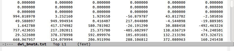
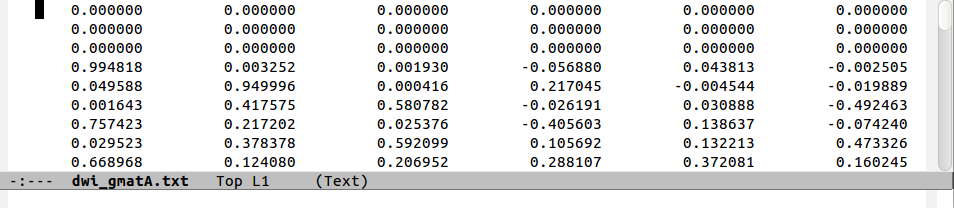
The following figure shows a comparison of the same few lines of b- and g- matrix and vector formats:

Grad/matrix selection	Style description
	(row, unit-magnitude) gradient file; note the arrows on the edge signifying that each line is actually wrapped over many rows of the text editor
	(row) b-value file; the single line is wrapped around to many rows in the text editor
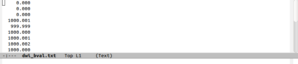
	(column) b-value file
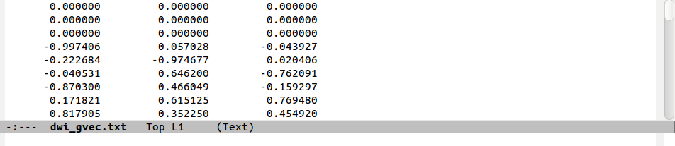
	(column, unit-magnitude) gradient file
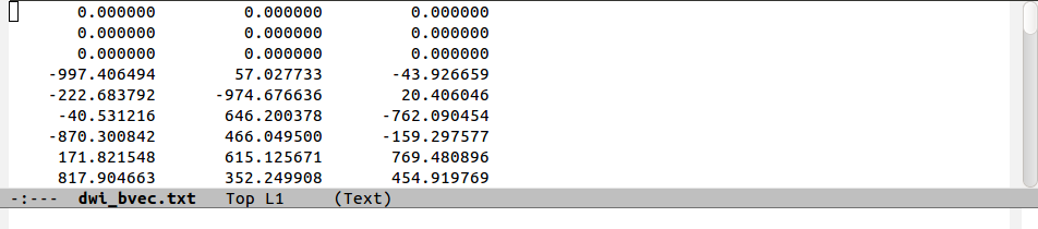
	(column, DW-scaled) gradient file
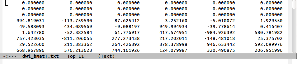
	row-first (TORTOISE-style) b-matrix; the three columns with no negative values contain the diagonal elements of the matrix; this has a different order and a factor of 2 scaling the off-diagonal elements, compared to the ‘AFNI-style’.
	diagonal-first (AFNI-style) b-matrix; the three columns with no negative values contain the diagonal elements of the matrix.
	row-first (AFNI-style) g-matrix

Note that in the ‘diagonal-first’ matrix case, the first three columns contain only non-negative ( $\geq0$ ) numbers. This will always be the case, since the b- or g-matrix is positive definite, and this property provides a solid hint as to the style of a given matrix output. (Columns of off-diagonal elements may or may not contain negatives). In the ‘row-first’ cases columns 0, 2 and 5 contain the matrix diagonals. The factors of two in the columns representing off-diagonal matrix elements is apparent when comparing the b-matrices. Finally, one can see how the b=1000 information translates into the b-matrix file by comparing the last two rows.

Note

This is discussed more below, but current recommendations for using AFNI DT-calculating functions (e.g., 3dDWItoDT and 3dDWUncert) is to make AFNI-style b-matrices.

We like the b-matrix format because we can use all of the rows when inputting into 3dDWItoDT or 3dDWUncert with the -bmatrix_FULL * option; gradient vector-based options would want one less row, just assuming that the 0th volume in the set is b=0, which might not be the case.
We like having DW scaling in the matrix info (the b-value), so that we preserve real physical units in the tensor estimates. When using 3dDWItoDT or 3dDWUncert, one should probably also use the -scale_out_1000 switch to have nice numbers, which are then interpreted as $10^{-3}~{\rm s~mm}^{-2}$ instead of the default ${\rm s~mm}^{-2}$ ; thus, the number part for average healthy adult parenchyma would be “0.7” (in units of $10^{-3}~{\rm s~mm}^{-2}$ ) rather than “0.0007” (in units of ${\rm s~mm}^{-2}$ ), which might be more annoying for bookkeeping/calculations.

7.2.2. Operations ¶

Note the name of the function, 1dDW_Grad_o_Mat++, which is now the recommended processor for gradient/matrix things in AFNI. It supercedes the older, clunkier 1dDW_Grad_o_Mat. The newer 1dDW_Grad_o_Mat++ has clearer syntax, better defaults and promotes world peace (in its own small way).

Gradient and matrix information ¶

The relevant formats described above can be converted among each other using 1dDW_Grad_o_Mat++. The formats of inputs and outputs are described by the option used, as follows:

input/option	style description	example program
-{in,out}_row_vec	row gradients	`dcm2niix` output, `TORTOISE` input
-{in,out}_col_vec	column gradients	basic input to `3dDWItoDT` (not preferred one, tho’)
-{in,out}_col_matA	row-first g- or b-matrices (user can choose scaling)	alt. input to `3dDWItoDT` (preferred!); (some, maybe) `TORTOISE` output
-{in,out}_col_matT	diagonal-first g- or b-matrices	(some/typical) `TORTOISE` output

Additionally, the file of b-values may be input after the -in_bvals * option. This might be requisite if converting gradients to b-matrices, for instance (but be sure not to scale up an already-scaled set of vectors/matrices!). One can input either a row- or column-oriented file here; 1dDW_Grad_o_Mat++ will know what to do with either one (because it will be 1-by-something or something-by-1). When outputting a separate file of b-values, one does have to specify either row or column, using: -out_row_bval_sep * or -out_col_bval_sep *, respectively.

The b-values can also be used to define which associated gradient/matrix entries refer to reference images and which to DWIs; if not input, the program will estimate this based on the magnitudes of the gradients– those with essentially zero magnitude are treated as reference markers, and the rest are treated as DWI markers. In general now, the distinction between reference and DW-scaled gradients is not very important: we no longer average reference volumes by default, and it probably shouldn’t be done.
In rare cases, one might want to include a column of b-values in the output gradient/matrix file. One example of this is with DSI-Studio for HARDI fitting. One can enact this behavior using the -out_col_bval switch. The first column of the text file will contain the b-values (assuming you either input b-matrices or used -in_bvals *). This option only applies to columnar output.
In contrast to the older 1dDW_Grad_o_Mat, the newer 1dDW_Grad_o_Mat++ does not try to average b=0 files or to remove the top row of reference volumes from the top of the gradient/matrix files. Nowadays, if one inputs a file with N reference and M DW images, the output would have the gradients/matrices of all $N+M$ . One major reason for preferring using the AFNI-style b-matrix as the format of choice is because the full set of $N+M$ values are used via the -bmatrix_FULL * option in 3dDWItoDT, 3dDWUncert, etc. (as opposed to $N+M-1$ ones if using grads or a difference b-matrix option, for historical reasons).

Simultaneous averaging of datasets ¶

This is not performed in ``1dDW_Grad_o_Mat++``. We no longer recommend doing this, based on the way tensor fitting is peformed.

How to check about gradient flipping?¶

The discussion of this specific topic has been moved to its own page, @GradFlipTest: checking on gradient flips. Please see there for the mathematical description of gradient flipping and tractographic images of its consequences, as well as the best way to investigate the phenomenon.

(The short answer is, “Use @GradFlipTest.”)

Example `1dDW_Grad_o_Mat++` commands ¶

Consider a case where dcm2niix has been used to convert data from a DWI acquisition, resulting in: a NIFTI file called ALL.nii.gz; a row gradient file called ALL.bvec (unweighted, unit magnitudes); and a (row) b-value file called ALL.bval. Let’s say that the acquisition aquired: 4 b=0 reference images; then 30 DW images with b=1000. Then:

The following produces a gradient file with 3 columns and 34 rows (unscaled, gradient vectors):

1dDW_Grad_o_Mat++                         \
   -in_row_vec   ALL.bvec                 \
   -out_col_vec  dwi_bvec.dat

The following flips the y-component of the input DW gradients and produces a row-first b-matrix (i.e., elements scaled by DW value) file with 6 columns and 34 rows:

1dDW_Grad_o_Mat++                         \
   -in_row_vec   ALL.bvec                 \
   -in_bvals     ALL.bval                 \
   -out_col_matA dwi_matA.dat
   -flip_y

An example of including @GradFlipTest's guess at an appropriate gradient flip in a pipeline with 1dDW_Grad_o_Mat++ is provided in “Combining with 1dDW_Grad_o_Mat++ (or fat_proc functions)”.

But be sure to also read “Caveats with @GradFlipTest” in order to appreciate the importance of still checking @GradFlipTest results by eye yourself (-> something that the function’s output assists with, anyways).
Sometimes, to deal with odd sequence protocol necessities, a single DW scaling is stored for each b-value and the gradients themselves are scaled to less than unity to reflect having a lower, applied weighting. Weird. But we can deal with this– the following example would combine the b-values and gradients, and then output gradient-magnitude (column) vector grads and the effective b-values separately:
```
1dDW_Grad_o_Mat++                         \
   -in_row_vec   ALL.bvec                 \
   -in_bvals     ALL.bval                 \
   -out_col_vec  dwi_gvec.dat             \
   -out_col_bval_sep dwi_bval.dat         \
   -unit_mag_out
```
The following first selects only some of the gradient and associated b-values (for example, if motion had occured). Of the original 34 volumes, this would select $4+1+22=27$ gradients, and similar subbrick selection would have to be applied to the set of DWI volumes:
```
1dDW_Grad_o_Mat++                         \
   -in_row_vec   ALL.bvec'[0..3,8,12..$]' \
   -in_bvals     ALL.bval'[0..3,8,12..$]' \
   -out_col_matA dwi_matA_sel.dat

3dcalc                                    \
   -a ALL.nii'[0..3,8,12..$]'             \
   -expr 'a'                              \
   -prefix ALL_sel.nii
```
Note

Subset selection works similarly as in other AFNI programs, both for datasets and the row/column files. For row text files, one uses square-brackets ‘[A..B]’ to select the gradients A to B. For column text files, one would do the same using curly brackets ‘{A..B}’.

7.2. 1dDW_Grad_o_Mat++: dealing with DW gradients¶

7.2.1. Overview ¶

Diffusion gradients ¶

Diffusion matrices ¶

7.2.2. Operations ¶

Gradient and matrix information ¶

Simultaneous averaging of datasets ¶

How to check about gradient flipping?¶

Example `1dDW_Grad_o_Mat++` commands ¶

Table of Contents

This Page

Quick search