HOW-TO #5
Across-Subjects Comparisons of FMRI Data -
Running Analysis of Variance (ANOVA) with AFNI 3DANOVA Programs
PART II: Running the ANOVA
The first script (Part I) of this how-to allowed us to process each subject's
dataset, in preparation for input into the ANOVA program. With these steps
completed, we are now ready to dive into the ANOVA. However, we must first
reorganize our data a bit, so that all relevant datasets for each subject are in
one directory, from which the ANOVA will be run. This second script
(@anova_ht05) will do all the reorganization that is necessary, and then run the
ANOVA. Once the ANOVA is completed, we will view the results in AFNI.
Outline of AFNI How-To #5, Script PART II:
-----------------------------------------
I. Organize the Datasets needed for the ANOVA
A. Create a new directory for the group analysis.
B. Use AFNI '3dcopy' to copy a Talairached, anatomical dataset from a
subject and move to the group analysis directory.
C. Copy the mean IRF datasets for each subject into the group analysis
directory.
II. Run a Two-Way Analysis of Variance with '3dANOVA2'
------------------------------------------------------------------------------
------------------------------------------------------------------------------
I. ORGANIZE THE DATASETS NEEDED FOR THE ANOVA
------------------------------------------------------------------------------
------------------------------------------------------------------------------
A. Create a new directory for the group analysis called "group_data"
----------------------------------------------------------------
Datasets necessary for the group analysis will be stored in this newly
created directory. In addition, the output dataset from the ANOVA will be
stored here. It is probably a good idea to create this new dataset at the
level of the parent directory, Points/. Just to reiterate, here is our
directory tree thus far and the datasets we'll need for the ANOVA:
cd Points
ls ED EE EF
ED/ EE/ EF/
ED_HM_irf_mean+tlrc.* EE_HM_irf_mean+tlrc.* EF_HM_irf_mean+tlrc.*
ED_TM_irf_mean+tlrc.* EE_TM_irf_mean+tlrc.* EF_TM_irf_mean+tlrc.*
ED_HP_irf_mean+tlrc.* EE_HP_irf_mean+tlrc.* EF_HP_irf_mean+tlrc.*
ED_TP_irf_mean+tlrc.* EE_TP_irf_mean+tlrc.* EF_TP_irf_mean+tlrc.*
EDspgr+trlc.*
To begin, run the script from the Points/ directory:
mkdir group_data
This "make directory" command will create a new directory called
'group_data', which can be found in our parent directory 'Points':
ls Points
ED/
EE/
EF/
group_data/
----------------------------------------------------------------------------
----------------------------------------------------------------------------
B. Use AFNI '3dcopy' to copy an anatomical dataset from one of the subjects
------------------------------------------------------------------------
COMMAND: 3dcopy
This program will copy AFNI datasets, using the old prefix and assigning a
new prefix.
Usage: 3dcopy [-verb] old_prefix new_prefix
(see also '3dcopy')
Why use '3dcopy' rather than the UNIX 'cp' command?
---------------------------------------------------
Each AFNI dataset has its own unique identifier code, located in the
header file. When '3dcopy' is used, the copied dataset recieves a brand
new ID code, even though the actual data is identical to it's parent
dataset. This is simply a nice way for AFNI to distinguish between
datasets. The 'cp' command does not create a new ID code for the copied
dataset. Therefore, AFNI will not be able to distinguish between the two
datasets (i.e., which is the original and which is the copy). It is good
practice to use '3dcopy' whenever possible. Of course, there are instances
when 'cp' is more practical (as we will see in step C below).
------------------------------------
* EXAMPLE of '3dcopy':
To view the results of the ANOVA, we will need to provide an anatomical
dataset that will serve as our "anatomical underlay" in AFNI. The
statistics from our ANOVA dataset will be the "functional overlay". In
this example, we will:
1. Descend into subject ED's directory.
2. Copy his Talairached anatomical dataset and give the copy a new
prefix name.
3. Move the copied dataset to our group_data/ directory.
4. Ascend into the group_data/ directory.
cd ED
3dcopy EDspgr+tlrc sample_anat+tlrc
mv sample_anat+tlrc.* ../group_data
cd ..
At this point, the only dataset in the group_data directory should be the
copied anatomical dataset:
ls group_data/
sample_anat+tlrc.HEAD
sample_anat+tlrc.BRIK
----------------------------------------------------------------------------
----------------------------------------------------------------------------
C. Copy each subject's Talairached, mean IRF datasets into the 'group_data'
directory
--------------------------
cp ??/??_??_irf_mean+tlrc.* group_data
In this case, it is much, much easier to simply 'cp' the IRF datasets into
the 'group_data' directory rather than run '3dcopy' for each one. Their
sole purpose is to be used for the ANOVA we will run in the 'group_data'
directory. Since the original IRF datasets are stored safely in each
subject's directory, we are simply using these copies for our analysis and
can delete them, if we wish, from the 'group_data' directory after the
ANOVA is completed.
------------------------------------------------------------------------------
------------------------------------------------------------------------------
II. RUN A 2-WAY ANOVA WITH AFNI '3dANOVA2'
------------------------------------------------------------------------------
------------------------------------------------------------------------------
COMMAND: 3dANOVA2
This AFNI program performs a two-factor analysis of variance (ANOVA) on 3D
datasets.
Usage: 3dANOVA2
-type k
-alevels a
-blevels b
-dset a b
[-options]
(see also '3dANOVA2 -help)
------------------------------------
* EXAMPLE of 3dANOVA2
In our sample experiment, we have two factors (or independent variables)
for our analysis of variance: "Stimulus Condition" and "Subjects". As
such, we are using the '3dANOVA2' program. The levels for each factor are
shown below:
a) Stimulus Condition --> 4 levels:
---------
Tool Movies
Human Movies
Tool Points
Human Points
b) Subjects --> n = 3:
------
Subject ED
Subject EE
Subject EF
Our script shows the following '3dANOVA2' command (don't panic, each
argument and option will be explained in detail):
3dANOVA2 -type 3 -alevels 4 -blevels 3 \
-dset 1 1 ED_TM_irf_mean+tlrc \
-dset 2 1 ED_HM_irf_mean+tlrc \
-dset 3 1 ED_TP_irf_mean+tlrc \
-dset 4 1 ED_HP_irf_mean+tlrc \
-dset 1 2 EE_TM_irf_mean+tlrc \
-dset 2 2 EE_HM_irf_mean+tlrc \
-dset 3 2 EE_TP_irf_mean+tlrc \
-dset 4 2 EE_HP_irf_mean+tlrc \
-dset 1 3 EF_TM_irf_mean+tlrc \
-dset 2 3 EF_HM_irf_mean+tlrc \
-dset 3 3 EF_TP_irf_mean+tlrc \
-dset 4 3 EF_HP_irf_mean+tlrc \
-amean 1 TM \
-amean 2 HM \
-amean 3 TP \
-amean 4 HP \
-acontr 1 1 1 1 AllAct \
-acontr -1 1 -1 1 HvsT \
-acontr 1 1 -1 -1 MvsP \
-acontr 0 1 0 -1 HMvsAP \
-acontr 1 0 -1 0 TMvsTP \
-acontr 0 0 -1 1 HPvsTP \
-acontr -1 1 0 0 HMvsTM \
-fa StimEffect \
-bucket AvgANOVAv1
------------------------------------
* EXPLANATION of '3dANOVA2' command in our script:
-type
This is a mandatory argument that must appear in the 3dANOVA2 command.
It tells the program the type of ANOVA model to be used. There are
three model types to choose from:
k=1 Fixed effects model (A and B fixed)
k=2 Random effects model (A and B random)
k=3 Mixed effects model (A fixed, B random)
What is the difference between a "fixed" and a "random" variable?
* FIXED:
We are only interested in gereralizing the results of our
study to experimental values used in the study. For instance,
a drug study might distribute 0 mg, 5 mg, or 10 mg of drug X.
The therapeutic effects of drug X in our study can only be
applied to drug X, with dosages of 0, 5, and 10 mg. We cannot
make inferences about the effects of drug X at 2 mg or 100 mg,
nor could we generalize the results to 0, 5, and 10 mg of
drug Y. We can only say that the results we obtained were
due to drug X, at 0 mg, 5 mg, and 10 mg because this is all
we tested for.
In our example, the "Stimulus Condition" variable with four
levels - "Tool Movies", "Human Movies", "Tool Points", and
"Human Points" - is a fixed variable. The brain activation
resulting from these stimuli can be applied only to those
conditions and not to other ones like "Human Drawings" or
"Tool Photographs".
* RANDOM:
The results or values obtained from a random variable are
assumed to be values that are drawn from a larger population
of values and thus, will represent them. "Subjects" are often
used as a random variable. In our example, subjects ED, EE,
and EF took part in our study, but they are subjects who come
from a larger population of people who share the same
demographics as these subjects. As such, the subejcts come
from a larger universe of potential subjects. Such a
generalization is more of an inferential leap, and
consequently, the random effects model is less powerful
statistically.
* MIXED:
A study consists of a mix of fixed and random variables. In
our study, "Stimulus Condition" is fixed, and "subjects" is
random. Therefore, we have a mixed effects model. In our
ANOVA command, we indicate this by selecting "3" as our "type"
(-type 3)
-alevels
This is a mandatory argument that asks for the number of levels for
our first factor. In this example, our factor 'a' is "Stimulus
Condition," with 4 levels (TM, HM, TP, HP). Therefore, -alevels = 4.
-blevels
This is a mandatrory argument that asks for the number of levels for
our second factor. In this example, our factor 'b' is "Subjects,"
with 3 levels (subjects ED, EE, EF). Therefore, -blevels = 3.
-dset a b filename
This mandatory argument gives the user an organized way to set up all
of the datasets that will be included in the ANOVA. In this example,
we have 4 stimulus conditions (TM, HM, TP, HP) and 3 subjects (ED, EE,
EF). Therefore, we have 12 IRF datasets we want to include in the
ANOVA. They will be labeled in the following manner:
SUBJECT (b)
ED EE EF
--- --- ---
TM 1,1 1,2 1,3
STIM.
COND. HM 2,1 2,2 2,3
(a)
TP 3,1 3,2 3,3
HP 4,1 4,2 4,3
----------------------------
1,1 = ED_TM_irf_mean+tlrc.*
2,1 = ED_HM_irf_mean+tlrc.*
.
.
.
3,3 = EF_TP_irf_mean+tlrc.*
4,3 = EF_HP_irf_mean+tlrc.*
-amean
This option estimates the mean for every level of factor 'a'. In our
example, factor 'a' (stimulus condition) has four levels. The '-amean'
option will compute a voxel-by-voxel mean for each stimulus condition,
collapsed across subjects. For instance, let's look at voxel "x" in
each level of factor 'a' for each subject:
Percent Signal Change at Voxel "x"
Factor 'b'
ED EE EF
Tool Movies 4.1% 3.8% 4.5% M = 4.13%
-------------------------------------
Factor Human Movies 3.2% 2.5% 2.8% M = 2.83%
'a' -------------------------------------
Tool Points 4.6% 4.1% 4.9% M = 4.53%
-------------------------------------
Human Points 1.7% 2.0% 1.1% M = 1.60%
-------------------------------------
For each voxel, the mean percent signal change for each stimulus
condition is collapsed across subjects and averaged. A t-statistic
also accompanies each mean. If a mean in a voxel is significantly
greater than zero, it appears as a color blob over the anatomical
image.
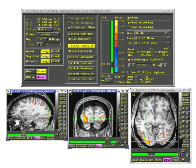
Figure 1 shows brain areas responding to the "Tools Movies" condition.
These areas show mean percent signal changes for the Tools Movies
condition, collapsed across subject, that are significantly greater
than zero. As predicted, the medial fusiform gyrus responded
significantly to the presentation of tool movies.
Figure 1. Brain Areas Responding to "Tool Movies"
--------------------------------------
 -acontr
This option is used to estimate a contrast in factor levels. In our
example, Factor "A" has four levels. Each of these levels can be paired
for a contrast to determine if their percent signal changes differ
significantly from each other throughout the brain. For example:
TM HM TP HP
-- -- -- --
0 1 0 -1 Compare Human Movies vs. Human Points
1 0 -1 0 Compare Tool Movies vs. Tool Points
0 0 1 -1 Compare Tool Points vs. Human Points
1 -1 0 0 Compare Tool Movies vs. Human Movies
Further contrasts can be made by collapsing across "object type" (i.e.,
humans vs. tools) and "animation type" (i.e., movies vs. points). For
instance, we can compare humans versus tools, irrespective of whether
they are presented as movies or points-of-light displays:
Tools Humans Movies Points
----- ------ ------ ------
1 -1 0 0 Compare Tools vs. Humans
0 0 1 -1 Compare Movies vs. Points
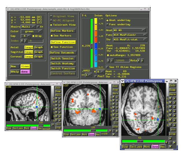
Figure 2 shows the results of a contrast between Movies versus Points.
As predicted, the ventral temporal cortex responded better to movie
displays (shown in reds) than point-light displays (shown in blues)
Figure 2. Contrast for Movies versus Point-Light Displays
----------------------------------------------
-acontr
This option is used to estimate a contrast in factor levels. In our
example, Factor "A" has four levels. Each of these levels can be paired
for a contrast to determine if their percent signal changes differ
significantly from each other throughout the brain. For example:
TM HM TP HP
-- -- -- --
0 1 0 -1 Compare Human Movies vs. Human Points
1 0 -1 0 Compare Tool Movies vs. Tool Points
0 0 1 -1 Compare Tool Points vs. Human Points
1 -1 0 0 Compare Tool Movies vs. Human Movies
Further contrasts can be made by collapsing across "object type" (i.e.,
humans vs. tools) and "animation type" (i.e., movies vs. points). For
instance, we can compare humans versus tools, irrespective of whether
they are presented as movies or points-of-light displays:
Tools Humans Movies Points
----- ------ ------ ------
1 -1 0 0 Compare Tools vs. Humans
0 0 1 -1 Compare Movies vs. Points
Figure 2 shows the results of a contrast between Movies versus Points.
As predicted, the ventral temporal cortex responded better to movie
displays (shown in reds) than point-light displays (shown in blues)
Figure 2. Contrast for Movies versus Point-Light Displays
----------------------------------------------
 -fa
This command produces a main effect for factor A. It determines if the
intensity in each voxel is significantly different from zero (F-stat)
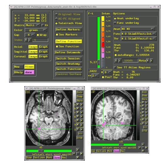
Figure 3 shows what the main effect for "Stimulus Condition" in our
sample study. The color blobs show brain activation in response to the
presence of a stimulus condition. These areas seem to respond to motion
stimuli in general.
Figure 3. Main Effect for "Stimulus Condition" Factor
-------------------------------------------
-fa
This command produces a main effect for factor A. It determines if the
intensity in each voxel is significantly different from zero (F-stat)
Figure 3 shows what the main effect for "Stimulus Condition" in our
sample study. The color blobs show brain activation in response to the
presence of a stimulus condition. These areas seem to respond to motion
stimuli in general.
Figure 3. Main Effect for "Stimulus Condition" Factor
-------------------------------------------
 -bucket
This option creates a "bucket" dataset, whose sub-bricks are obtained by
concatenating all of the output files created by the ANOVA. In this
example, the bucket dataset "AvgAnovav1" will contain the 26 sub-bricks,
consisting of the main effect of Factor "A", means for each of the four
levels of Factor "A", and results from our contrasts. This bucket
dataset can be found in the group_data directory:
cd Points/group_data
AvgAnova1+tlrc.HEAD
AvgAnova1+tlrc.BRIK
------------------------------------------------------------------------------
CONGRATULATIONS! YOU HAVE REACHED THE END OF HOW-TO #5.
For more information on AFNI ANOVA programs, refer to Doug Ward's paper on
Analysis of Variance for FMRI data, located on the AFNI website at
3dANOVA.ps.
-bucket
This option creates a "bucket" dataset, whose sub-bricks are obtained by
concatenating all of the output files created by the ANOVA. In this
example, the bucket dataset "AvgAnovav1" will contain the 26 sub-bricks,
consisting of the main effect of Factor "A", means for each of the four
levels of Factor "A", and results from our contrasts. This bucket
dataset can be found in the group_data directory:
cd Points/group_data
AvgAnova1+tlrc.HEAD
AvgAnova1+tlrc.BRIK
------------------------------------------------------------------------------
CONGRATULATIONS! YOU HAVE REACHED THE END OF HOW-TO #5.
For more information on AFNI ANOVA programs, refer to Doug Ward's paper on
Analysis of Variance for FMRI data, located on the AFNI website at
3dANOVA.ps.