1	Using the Volume Rendering Plugin Accessed via Define Datamode ---> Plugins ---> Render [new]
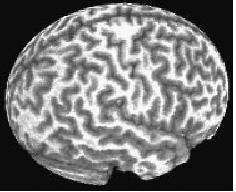
2	"Volume rendering concepts:" Volume rendering concepts: Goal is to create a 2D image consisting of pixels Each 2D pixel is obtained from data looking down line of sight into 3D volume:
3	"Opacity examples:" Opacity examples: start with (remaining) opacity of 1, and apply a fraction of it at each new voxel
4	"3D viewing angles:" 3D viewing angles: Roll = angle about I-S axis Pitch = angle about L-R axis (after roll rotation) Yaw = angle about A-P axis (after roll and pitch) Rendering is CPU and memory intensive --- a fast computer is very desirable Utility program 3dIntracranial can be used to strip the scalp off of a T1-weighted anatomical volume. In some cases, this may need to be done with the orig dataset, which may then be written out in Talairach coordinates. For example: 3dIntracranial -anat anat+tlrc -prefix astrip AFNI can now render datasets that are stored with an arbitrary orientation and voxel size Datasets are internally re-oriented (see 3dresample) to axial slice order, so that cut directions make sense. This may take a few seconds, depending on the computer. Note that axial slice order is the standard for ‘warped’ datasets written out to disk in +acpc or +tlrc coordinates. The Overlay dataset may also be resampled, so that its grid spacing matches that of the Underlay dataset.
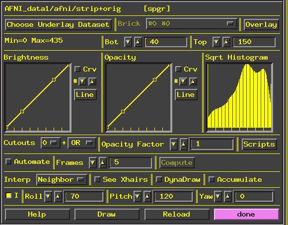
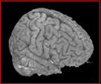
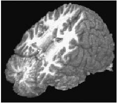
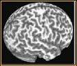
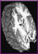
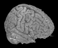
5	"In Talairach view," In Talairach view, open the rendering plugin, and choose astrip+tlrc as the underlay dataset Plugin will load the voxel values, build the histogram, and then be ready to render Press Draw to make your first image Press Accumulate, then DynaDraw, then Roll t a few times Will generate renderings from different angles (i.e., lines of sight) If DynaDraw is off, then you must press Draw to get a new rendering Accumulate on Þ rendered images are saved, and can be reviewed by using the image viewer slider This slider does not move you through slices, as it does in the 2D image viewing windows It just moves you backward and forward in the history of saved rendered images If you turn Accumulate off, then creating the next rendered image will erase the history By default, the plugin’s controls (‘widgets’) do not change as you move around in the rendering history Selecting ScriptàLoad widgets will make the widgets display the settings they had when the currently displayed image was rendered
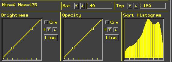
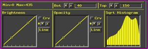
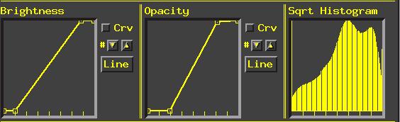
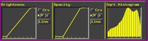
6	"Controlling the mappings from voxel..." Controlling the mappings from voxel value to brightness and opacity:
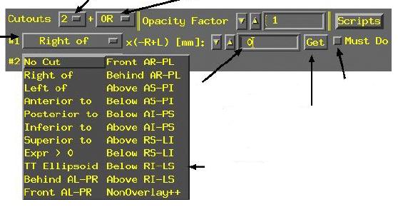
7	"Cutouts are for removing parts..." Cutouts are for removing parts of the volume so you can see the parts you want:
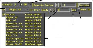
8	"Most cutout types are controlled..." Most cutout types are controlled by a single numerical parameter determining the position of the cutout Right of ’x’ means to cut out all voxels to the right of the given x-coordinates (-x is Right, +x is Left) Similarly, can cutout everything Anterior to, Posterior to, or Superior to, Inferior to, or Left of a given coordinate position Behind…, Below…, Front…, Above… cut out 45^o diagonally slanted half-spaces, with respect to the listed planes: For example, Above AS-PI is above a plane that slants from the Anterior-Superior front of the brain downwards to the Posterior- Inferior back of the brain -- that is, halfway between a coronal and axial slice TT Ellipsoid cuts out the region outside an ellipsoid with the same proportions as the Talairach-Tournoux Atlas brain This is fun, but not much use
9	"Cutout type Expr > 0..." Cutout type Expr > 0 defines the region to be removed by a general mathematical expression, rather than a single parameter The expression uses the same syntax as 3dcalc Variables that can be used are ‘x’, ‘y’, and ‘z’, corresponding to spatial coordinates in the dataset When using Automate (infra), variable ‘t’ can also be used The (x, y, z) locations where the expression evaluates to a positive number will be cut out 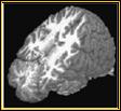Example: rendering a slab tilted at an arbitrary angle between coronal (xz-plane) and axial (xy-plane):
10	"The set of points within..." The set of points within the slab is described by the inequality ïy · cos(a) - z · sin(a) -sï < 1/2w for angle=a, slab center offset=s, and slab width=w. To render a slanted coronal slab 30 mm thick, tilted posteriorly from the vertical of 25^o, we would use this for the cutout expression: abs(ycosd(25)-zsind(25)-20)-15 where the sind() and cosd() functions take arguments in degrees, and where the offset has been set to 20 mm (you will have to alter this offset to get the exact position you want) By using Automate and setting the angle (25 above) and/or the offset (20 above) to depend on ‘t’, we can make a sequence of images where the slab rotates downwards and/or moves backwards
11	"Automate lets you create a..." Automate lets you create a large number of renderings at once Note that most (but not all) number entry boxes have slightly raised borders:
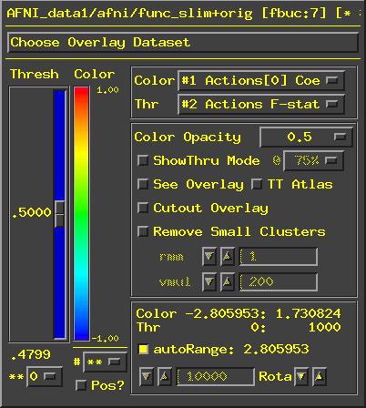
12	"Color overlays (e.g.,..." Color overlays (e.g., of functional activation maps) Press the [Overlay] button to open up the panel that controls how functional overlays are generated:
13	"Color Opacity lets you select..." Color Opacity lets you select the opacity of colored voxels (those that are above the threshold) Opacity of overlaid voxels is different from the opacity it would have from the underlay dataset at that location Usually want this to be high (0.5 or above) Tow special values on this menu: Underlay means that the colored voxel’s opacity will be determined by the opacity that it would have from the underlay image 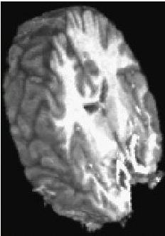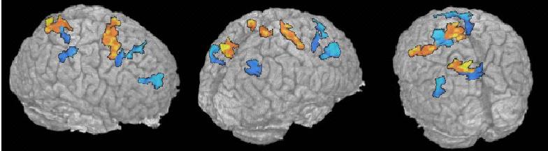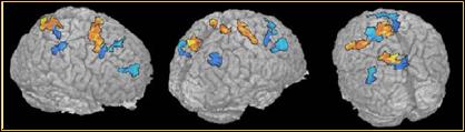ShowThru means that colored voxels show through underlay voxels (the ‘glass brain’ effect), no matter how opaque the underlay is Takes some practice to become accustomed to this type of image But can be a very useful way to see lots of activation at once: