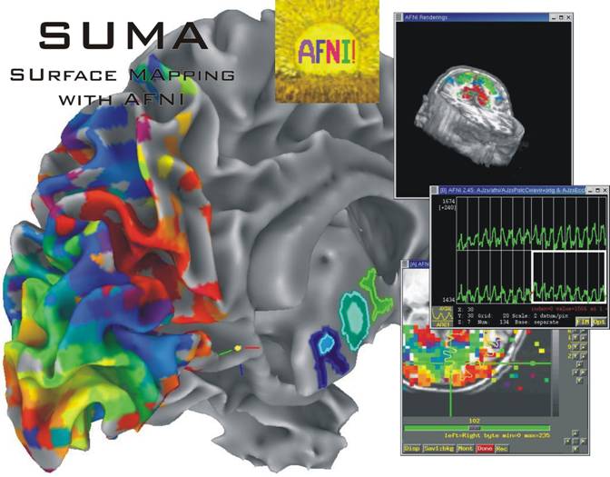
I. SUMA (SUrface MApping)
SUMA is a program that adds cortical surface based functional imaging analysis to the AFNI suite of programs http://afni.nimh.nih.gov . SUMA allows the viewing of 3D cortical surface renderings, the mapping of volumetric data onto them and, in future incarnations perform surface based computations and statistical inferences. With SUMA, AFNI can simultaneously and in real-time render Functional Imaging data in 4 modes: Slice, Graph (time series), Volume and Surface. SUMA supports surface models created by FreeSurfer http://surfer.nmr.mgh.harvard.edu/ and SureFit http://stp.wustl.edu/resources/surefitnew.html programs.
(Download this manual in PDF format.)
A. Highlights:
1. Surface rendering with direct AFNI link:
2. Multiple Linked Viewers:
You can have up to 6 linked surface viewers open simultaneously.

3. ROI Drawing:
Free hand ROI drawing in any viewer.

4. Simultaneous left / right hemisphere display:
5. Talairach surface and volume:
If your volumetric data are in Talairach space, you can display them on these surfaces.

6. Control of dataset color mapping (color plane) order and opacity:
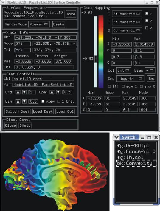
Each dataset is colored interactively using SUMA’s surface controller shown below. The color mapping of each dataset is stored in a separate color plane whose order and opacity can be controlled for each surface model. The image below shows surface models with 4 stacked color planes consisting of the surface convexity, drawn ROIs, functional data from AFNI and a node color data file that looks cool.
7. Recording in continuous and single frame modes:
Rendered images can be captured by an AFNI-esque image viewers and saved into all formats provided by AFNI, including animated gifs and mpegs.
8. A set of command line programs for batch processing:
a. Volume to surface & surface to volume mapping:
Command line programs for mapping surface-domain data into volume-domain and vice versa. Many options are provided for controlling the manner in which the mapping is done.
b. Filtering:
Command line program for smoothing surface geometry or smoothing data on the surface.
c. Miscellaneous:
Various programs for surface checking, editing and metrics and more.
B. Test-drive
Before delving into the details of using SUMA, try the following to get a feel for it. I assume that SUMA and SUMA_demo have been installed (see http://afni.nimh.nih.gov/ssc/ziad/SUMA/SUMA_Installation.htm ).
1. Nomenclature:
All button and mouse action must be initiated with the mouse cursor inside of the rendering window.
>
sign represents a command on the unix command line. Text in italics
represents comments.
>FS>
commands for FreeSurfer demos
>SF>
commands for SureFit demos
>SUMA>
commands or actions executed in SUMA's window
>SHELL>
commands or actions executed in SUMA's shell
>AFNI>
commands or actions executed in AFNI
Commands
following > may appear split in the documentation but they should be typed
on one line.
SUMA_demo refers to the demo directory obtained when archive SUMA_demo-FS.tgz or SUMA_demo-SF.tgz was installed.
2. Showcase:
- Launching SUMA:
> cd SUMA_demo/afni
> afni -niml &
>FS> suma -spec ../SurfData/SUMA/DemoSubj_lh.spec -sv DemoSubj_SurfVol_Alnd_Exp+orig
>SF> suma -spec ../SurfData/SURFACES/DemoSubj_lh.spec -sv DemoSubj_SurfVol_Alnd_Exp+orig
(NOTE: It used to be that you could not run SUMA in the background because you needed the terminal for input. That is no longer the case.)
You should see a surface model in SUMA's window by now. Minimize AFNI for the moment to keep it out of the way.
- Rotating the surface:
>SUMA> Mouse button-1: keep it down while moving the mouse left to right. This rotates the surface about the screen's Y-axis (dotted green). Let go of button-1. Repeat with up and down motion for rotation about X-axis and motion in various directions for rotations mimicking those of a trackball interface. Also try up/down/left/right arrow keys.
- Translating the surface:
>SUMA> Mouse button-2: keep it down while moving the mouse to translate surface along screen X and Y axes or any combinations of the two.
- Zooming in/out:
>SUMA> Both buttons 1&2 or Shift + button 2: while pressing buttons, move mouse down or up to zoom in and out, respectively. Also try keyboard buttons 'Z' and 'z' for zooming in and out, respectively.
- Cardinal views:
>SUMA> ctrl + Left/Right: Views along LR axis
>SUMA> ctrl + Up/Down: Views along SI axis
>SUMA> ctrl + shift + Up/down: Views along AP axis
>SUMA> Mouse button 3: press over a location on a surface to pick the closest node to the location of the cursor, the Facet that contains the picked location. Note the information written to the shell of the properties of the picked Node and Facet.
- Linking to AFNI:
If you have not yet launched AFNI, launch it from a separate shell in SUMA_demo/afni directory using the command:
> afni -niml &.
>SUMA> Press 't' with the cursor inside SUMA's window. If the communication is established, afni will acknowledge the receipt of the surface's Nodes and Facet Indices. Messages and errors are also output to the SUMA.
>AFNI> Switch Anatomy to DemoSubj_SurfVol_Alnd_Exp+orig and open an axial view. You will see a trace of the intersection of the surface with the anatomical slices displayed. You will also see boxes representing the nodes that are within +/- 1/2slice from the center of the slice in view (colors can be changed to suit your fancy. See Define Datamode --> Misc --> Edit Environment --> AFNI_SUMA* variables).
>SUMA> Right Click on the surface and watch the cross hairs pinpoint the same location in AFNI.
>AFNI> Left Click in the AFNI slice window and watch the cross hairs specify the location on the surface. If you don't see the cross hairs on the surface, they may be hidden on a fold or on the other side of the surface.
- Displaying Function:
>AFNI> Switch Function to DemoSubj_EccCntavir.DEL (Choose the functional data set)
>AFNI> Define Function --> Thr (middle right) to #2 Corr. Coef (Set up the color mapping)
>AFNI> Pos ON (below color bar)
(Only positive values mapped to color)
>AFNI> # (below color bar) to 20 (20 colors cyclical colormap. You need afni v. 2.49a or newer.)
>AFNI> See
Now you
should see function overlaid on the anatomical slice image and on the surface
model.
- Switch Viewing States:
>SUMA> '.' switches to the next viewing state (pial then inflated etc.)
>SUMA> ',' switches to the previous viewing state
>SUMA> Navigate on surfaces and watch AFNI track cross hair on surface
>AFNI> Change threshold in AFNI and watch map change on surface
When you're done playing, go to the inflated view and put some color on the surface.
- Back to Reference Surface
>SUMA> with inflated view shown, 'spacebar' to go from current view to mapping reference view and vice-versa. That's useful in orienting yourself when you're lost on a deformed surface. Note the correspondence of the cross hair's location. Stay in the inflated viewing state.
- Color manipulation:
>SUMA> 'a' toggle functional overlay attenuation by sulcal highlights (dark and bright colors highlight fundus and crown of gyrus, respectively).
>SUMA> 'b' toggle sulcal highlights
>SUMA> 'f' toggle functional overlay
- Momentum:
>SUMA> 'm' to toggle momentum to ON state. Press button-1 and while moving the mouse to rotate the surface, let go of button-1 (This takes a bit of practice, use faster mouse movement for faster turning). The surface should continue rotating in the mouse's direction when the button was released. Change functional data threshold or rotate color maps in afni and watch the updates occurring as the surface is tumbling in space. Pretty cool 'ey? Change viewing states. To stop momentum rotation, press 'm' again.
- Writing the scene to an image file:
>SUMA> 'r' to record the rendered image to an AFNIesque window which will allow you to save the image into different formats. The resolution of the saved image depends on the size of the SUMA window when the image is recorded: Bigger is better.
- Help:
>SUMA> 'h' to output help message to shell from which SUMA was launched.
C. Setting up surfaces and volumetric data:
This section shows how to prepare surfaces created by either FreeSurfer or SureFit for reading into SUMA and mapping FMRI data onto the cortical surface. All the examples are based on the data provided in SUMA_demo. If you want to run the commands shown here (highly recommended) you need to make a fresh copy of the demo directory. To do so run the following commands:
> cd SUMA_demo
> mkdir ../SUMA_MyDemo
> cp
-rp ./* ../SUMA_MyDemo
> cd
../SUMA_MyDemo
> rm
-f ./afni/DemoSubj_SurfVol*
>FS>
rm -rf ./SurfData/SUMA
>SF>
rm -rf ./SurfData/SURFACES/DemoSubj*spec
1. A- Surface Specification File:
This step is only needed when new surfaces are created.
----------------------------------------------------------------------------
a. In a nutshell:
Sample command summary for the impatient and/or the experienced:
These commands can be executed on the demo data.
> cd
SUMA_Mydemo/SurfData
>FS>
@SUMA_Make_Spec_FS -sid DemoSubj
or
>SF> @SUMA_Make_Spec_SF -sid DemoSubj
In the demo, choose 1 for both .L and .R because
they are the final corrected fiducial surfaces.
Choose 1 for LPI BRIK because that's the one used in creating the data set.
-----------------------------------------------------------------------------
b. The skinny:
Since SUMA supports surfaces created by various programs, one needs to define the relationship between different surfaces and provide information to link the surfaces to the volumetric data from which they were created. These relationships are defined in a Spec file that is automatically created for FreeSurfer and SureFit surfaces and can also be manually created/edited for advanced uses.
i. Creating the specs file for FreeSurfer:
Requirements:
- mris_convert (part of FreeSurfer distribution)
- to3d (part of AFNI distribution)
>FS> cd SubjDir
SubjDir is the directory where FreeSurfer's subdirectories (mri, surf, orig, etc.) are located.
>FS> @SUMA_Make_Spec_FS -sid SubjID
SubjID is an identifier for the subject.
The script will create ASCII versions of the left and right hemisphere surfaces. By default, the following surfaces are processed: smoothwm, pial, inflated, occip.patch3d, occip.patch.flat, sphere. If you are using other naming conventions or you want to add more surfaces, you will need to tailor the script to your needs. See section @SUMA_Make_Spec_FS for more details. All the .asc files and the Spec files DemoSubj_lh.spec and DemoSubj_rh.spec are placed in SubjDir/SUMA directory.
@SUMA_Make_Spec_FS will also create the Surface Anatomy Volume, in AFNI's data set format, out of the .COR images used for creating the surface. The output, DemoSubj_SurfVol+orig is placed in SubjDir/SUMA directory.
At this stage you should verify that the surfaces align with the Surface Anatomy Volume. Test it by running:
>FS> cd SubjDir/SUMA
>FS> afni -niml &
>FS> suma -spec SubjID_lh.spec -sv SubjID_SurfVol+orig
In the suma window, press 't' on the keyboard and watch afni acknowledging the receipt of the surface info. You will then see the contours of the left hemisphere overlapping with the gray/white matter boundary of the cortical surface. If the alignment is off, the most likely mistake is a wrong labeling of the left and right hemispheres.
If the labeling is correct, i.e. what you're calling left is the subject's left side of the brain. Then your coronal images may be in neurological convention (left is left) and you need to use the -neuro option with @SUMA_Make_Spec_FS. By default we assume that the .COR images are in RSP order.
ii. Creating the spec files for SureFit:
Requirements:
- to3d (part of AFNI distribution)
>SF> cd SubjDir (SubjDir is the directory where SureFit's afni volume and SURFACES directory are located.)
>SF> @SUMA_Make_Spec_SF -sid SubjID
SubjID is an identifier for the subject.
With Surefit, there are numerous versions of the
same surface with various degrees of corrections. You must choose the best one
from the list. It is usually the first one because the list is presented with
the most recent surface (based on the file's time stamp)first.
NOTE: Before creating our surface models using SureFit, we resampled and reoriented our anatomical volume to the desired 1mm3 resolution and LPI orientation. This simplified the process of creating the surfaces with SureFit and kept a record of volume manipulation in the volume's header file. We recommend you do the same using the new afni program 3dresample:
>SF> 3dresample -rmode Cu -orient LPI -dxyz 1.0 1.0 1.0 -prefix SubjID_SurfVol -inset AnatVol+orig
At this stage you should verify that the surfaces align with the Surface Anatomy Volume. Test it by running:
>SF> cd SubjDir
>SF> afni -niml &
>SF> cd SURFACES
>SF> suma -spec SubjID_lh.spec -sv SubjID_SurfVol+orig
In the suma window, press 't' on the keyboard and watch afni acknowledging the receipt of the surface info. You will then see the contours of the left hemisphere. If the alignment is off, the most likely mistake is the use of a wrong .params file or Surface anatomy volume.
2. B- Alignment of Surface to Experimental Data
This step is needed with each new experiment
----------------------------------------------------------------------------
a. In a nutshell:
Sample command summary for the impatient and/or the experienced:
These commands can be executed on the demo data.
> cd
SUMA_MyDemo/afni
>FS>
@SUMA_AlignToExperiment DemoSubj_spgrsa+orig
../SurfData/SUMA/DemoSubj_SurfVol+orig
>SF>
@SUMA_AlignToExperiment DemoSubj_spgrsa+orig
../SurfData/SURFACES/DemoSubj_SurfVol+orig
-----------------------------------------------------------------------------
b. The skinny:
To align a cortical surface model with data from a new experiment we align the anatomical volume used in creating the cortical surface (SurfVol) to the one in alignment with the experimental data (ExpVol). The process is illustrated in Figure 2 below. In most cases, the surface is created from data collected in different sessions from the experimental data and the alignment transform (Alignment Xform) is obtained by aligning SurfVol to ExpVol using 3dvolreg. It is worth noting that it is the Surface that is brought into alignment with the data and not vice-versa. Repositioning the surface comes at no cost while repositioning functional data requires spatial interpolation, which can alter the topology of the activation pattern on the surface. The output of 3dvolreg is a version of the Surface Anatomy Volume that is aligned with the Experiment anatomy volume and the alignment transform is stored in the aligned volume's header.
NOTE: Since SurfVol and ExpVol must be registered together, it is important that the two volumes exhibit comparable contrast. However they need not have the same resolution or SNR levels.
Figure 1: Aligning the surface to experimental data.
Figure 2: Mapping volumetric data onto surface
This figure is similar to Figure 1, along with volumetric data mapped onto the surface models to give you an idea of the complete process.
This procedure is implemented in the script @SUMA_AlignToExperiment (which requires 3dvolreg distributed with AFNI versions newer than 2.45l).
> cd SubjDir/afni
(this is the directory containing the functional imaging data to be mapped onto the surface)
>
@SUMA_AlignToExperiment ExpVol+orig SurfDir/SurfVol+orig
(SurfDir is the directory containing the volume
used in creating the surface.)
The output of @SUMA_AlignToExperiment is SurfVol_Alnd_Exp+orig. This data set is the Surface Volume data set aligned with the experiment's anatomical data set ExpVol+orig . See section @SUMA_AlignToExperiment for more info. It is very important to verify that the alignment of the two volumes is proper.
To do so:
> afni &
>AFNI> Switch Anatomy to DemoSubj_spgrsa+orig
>AFNI> Open an Axial Image
>AFNI> Open a new AFNI controller with New (locate lower left)
>AFNI> Switch Anatomy to DemoSubj_SurfVol_Alnd_Exp+orig
>AFNI> Open an Axial Image
(Make sure that both controllers are locked)
>AFNI> Define Datamode --> Lock --> Set All
>AFNI> Lock --> Enforce
( Make sure that Lock --> IJK Lock is NOT turned on)
>AFNI> Click in one of the axial windows and you should see the cross hairs move to a corresponding location in the other data set. Note the quality of alignment despite markedly different scan types, qualities and coverage.
3. C- Running SUMA
This step is needed each time you want to view the data on the cortical surfaces.
----------------------------------------------------------------------------
a. In a nutshell:
Sample command summary for the impatient and/or the experienced:
These commands can be executed on the demo data.
> cd
SUMA_MyDemo/afni
> afni
-niml &
>FS>
suma -spec ../SurfData/SUMA/DemoSubj_lh.spec -sv DemoSubj_SurfVol_Alnd_Exp+orig
or
>SF>
suma -spec ../SurfData/SURFACES/DemoSubj_lh.spec -sv
DemoSubj_SurfVol_Alnd_Exp+orig
-----------------------------------------------------------------------------
b. The skinny:
To run suma, execute the following:
> cd
SUMA_MyDemo/afni
> afni
-niml &
> suma
-spec SurfDir/SubjID_lh.spec -sv SubjID_SurfVol_Alnd_Exp+orig
SurfDir is the directory containing the Spec
files.
NOTE: Do not run the last command line in the background. SUMA needs the shell for interactivity with the user. If you need to run other programs, do so from another shell.
NOTE: SUMA assumes that the surfaces are in the same directory as the Spec File.
SUMA will load all the surfaces specified in the spec file and will show the Mapping Reference surface first as illustrated in Figure 3 below. Also shown are the screen (or eye) axes (dotted) and the surface axes (solid). Screen axes are attached to the screen and are mostly used to assist in illustrating surface rotations. Surface axes are bound to the surface and indicate the dicom orientations as used in AFNI's RAI (Right to left, Anterior to posterior and Inferior to superior orientations). By convention, XYZ axes are represented by the three colors Red, Green and Blue. Also shown in the cross hair that is formed of its 3 axes, a triangle highlighting the selected Facet, a blue sphere highlighting the selected Node and a yellow sphere highlighting the exact location of the cross hair's center on the intersected Facet.

Figure 3: Detail of cross-hair
D. Interacting with SUMA
The interaction with SUMA is currently through the mouse, keyboard and the shell (terminal) from which suma was launched.
1. SUMA viewer title:
The title of a viewer might look something like:
[B] SUMA:xR: lh.smoothwm.asc & rh.smoothwm.asc
which is broken down to the following parts:
[B]: indicates the viewer number (#2), you can open up to 6 viewers [A..F]
:xR: indicates which sides are shown in the display. The first character (after the ‘:’) is for the left side and the second is for the right side. ‘x’ means no surface present in this view. ‘h’ means a surface is present in this viewing state but hidden from view (see ‘[‘ / ‘]’ keys). ‘L’ means Left hemisphere displayed, ‘R’ means right hemisphere displayed. Example: :xR: means no left hemisphere surface in this view, right hemisphere version is visible. :Lh: means left hemisphere is visible, right hemisphere is hidden from view.
:Rec: indicates, if present, that viewer is in recording mode (see ‘R’ key).
lh.smoothwm.asc & rh.smoothwm.asc: list of surfaces in
the viewer in that viewing state.
2. Viewer Menus:
a. File Menu:
i. Save View:
Save viewer's display settings. Use this when you need to recall at a later time the manner in which the surface was displayed.
ii. Load View:
Load and apply display settings.
iii. Close:
Close this viewer.
Exit SUMA if this is the only viewer. Same as Escape key.
b. View Menu:
i. SUMA Controller:
Open SUMA controller interface.
ii. Surface Controller:
Open selected surface's controller interface.
iii. Viewer Controller:
Open viewer's controller interface.
iv. Cross Hair:
Toggle cross hair display (see also Figure 3).
v. Node in Focus:
Toggle highlight of selected node (see also Figure 3)
vi. Selected Faceset:
Toggle highlight of selected faceset (see also Figure 3).
c.
Tools Menu:
i. Draw ROI:
Open Draw ROI controller.
d.
Help Menu:
d.
i. Usage:
Opens window with usage help.
ii. Message Log:
Opens window containing errors and warnings typically output to screen.
iii. SUMA Global:
Output debugging information about some of SUMA's global
structure's variables.
iv. Viewer Struct:
Output debugging info on a viewer's structure.
v. Surface Struct:
Output debugging info on the selected surface's struct.
vi. InOut Notify:
Turn on/off function in/out tracing.
vii. MemTrace:
Turn on memory tracing. Once turned on, this can't be turned off.
3. Mouse Controls:
To confuse the user and satisfy the needy, you can swap the functions of mouse buttons 1 and 3 with an environment variable.
Also, mouse button functions can change when SUMA is in Draw ROI mode.
a. Button 1&Motion:
Rotation about the screen's axes (not the surface's axes). Rotation mimics the feel of a trackball (with the surface model inside of it). Rotations are about the screen's axes and not the surface's axes. Pure vertical motion is a rotation about the X-axis and is equivalent to using the up/down arrow keys. Pure horizontal motion is a rotation about the Y-axis is equivalent to using the left/right arrow keys.
b. Button 2&Motion:
Translation along screen axes.
c. Button 1+2&Motion or Shift+Button2 & Motion:
Zoom in/out. If you move the mouse down (towards you) you zoom in on the surface, if you move the mouse up (away from you) you zoom out.
d. Button 3-Press:
Crosshair positioning, Node and Facet picking.
e. Shift+Button3-Press:
Node and Facet picking when in Draw ROI Mode.
4. Keyboard Controls:
Keyboard controls are listed alphabetically and divided into two groups: Basic and Advanced. Basic commands may be of use to commoners and Advanced commands may be of use to developers.
a. a : attenuation by background, toggle.
Toggles color attenuation by the sulcal highlights.
b. 'b': background color, toggle.
Toggles sulcal highlights. The highlights represent convexity of the Mapping Reference Surface. Bright and dim highlights indicate crown and fundus of a gyrus, respectively.
c. ‘B’: Backface culling, toggle.
Toggles backface culling. Hidden patches are not rendered with backface culling on. Effect is most visible in wire mesh display mode.
d. 'c': node color file
Expects the name of an ASCII file with 4 tab-separated values per line:
NodeIndex R G B. Take care that no node index in this file is larger than N_Node -1. With N_Node being the total number of nodes of the surface in the viewer. R G B values must be between 0 and 1. This allows users to color the surface directly whichever way they please. The node colors in that file are placed in their own color plane which can be controlled via the surface controller.
e. ‘Ctrl+d’: draw ROI controller
Launches the Draw ROI
GUI.
f. 'F': Flip light position
Some surfaces are correctly lit with light from the +z direction (default) and others are best lit from the -z direction. This button toggles light position between the two positions. If you change the light position, this key will invert each of the three coordinates.
g. 'f': functional overlay, toggle.
Toggles functional overlay colors.
h. ‘H’: Highlights a set of nodes inside a box
Highlights nodes that fall inside a box of user specified
center and dimensions. Highlighting is done on SO in Focus only, other viewers
are not affected. Highlighting overwrites pre-existing colors and is wiped out
with a new color refresh.
i. ‘h’: No longer used, use ‘ctrl+h’ instead.
j. 'Ctrl+h': help message
Writes a help message to a searchable window.
k. ‘J’: Jump to faceset n on Surface Object (SO) in Focus.
The faceset of index n is highlighted as if it were selected by a mouse click. Other viewers and AFNI, if connected, are not affected. Crosshair’s location is not changed
l. ‘j’: jump to node n on SO in Focus
The node of index n is highlighted as if it were selected by a mouse click. Linked viewers and AFNI are also affected. Crosshair’s location is centered no node n.
m. ‘Ctlr+j’: jump to XYZ location
The cross hair is moved to coordinates XYZ. Other viewers, and AFNI are updated.
n. ‘Alt+j’: jump to node n on SO in Focus.
The node of index n is highlighted as if it were selected by a mouse click. Other viewers, AFNI and crosshair are not affected.
o. ‘L’: Light’s XYZ coordinates.
Set the light’s coordinates relative to the screen’s axes.
Default is 0,0,1 only direction matters.
p. 'l': look at point X,Y,Z
Reposition the surface such that the point about the center of the screen has coordinates XYZ.
q. ‘Ctrl+l’: lock mode switch
Switch locking mode of viewers between: No Lock, Index Lock and XYZ Lock. The switching order is relative to the lock on the first viewer. For finer lock control, use the SUMA Controller.
r. ‘Alt+l’: look at crosshair location
Reposition the surface such that the crosshair is about the
center of the screen. This version is very useful when combined with the ‘j’ key options.
You can use it to locate a certain node on the surface quickly.
s. 'm': momentum ON/OFF, toggle.
Toggles momentum to surface rotation. Momentum allows the surface to continue rotating after you let go of button-1 as you're still moving the mouse. Momentum is turned off initially and is activated when 'm' is pressed. Momentum may not be terribly useful but it is really cool.
t. ‘Alt+Ctrl+M’: Dumps memory trace to file .
Dumps memory trace to file called malldump.NNN where NNN is
the smallest number between 001 and 999 that has not been used.
u. ‘Ctrl+n’: new SUMA viewer .
Opens a new SUMA viewer window. You can have up to six
viewers open simultaneously.
v. ‘p’: viewer rendering mode.
Switches rendering mode between shaded, mesh and points. All
surfaces in viewer are affected, to control individual surface rendering modes,
use RenderMode
option in Surface Controller.
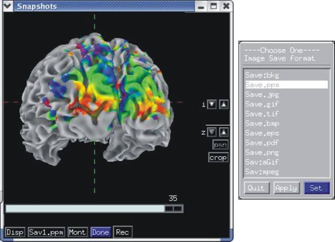
w. ‘r’: record the current image.
Records the current rendering to an image that gets stored in an AFNIesque viewer. You can save the images later in any of the AFNI supported formats. This function supersedes the troubled ‘w’ option. The AFNI recorder will reject duplicate consecutive images.
x. ‘R’: Record continuously, toggle.
Records all subsequent rendered images to an AFNIesque
viewer. You can save the resultant movie as an mpeg, animated GIF or any other
format supported by AFNI. The SUMA title bar shows :Rec: when in recording
mode. The AFNI recorder will reject duplicate consecutive images.
y. ‘Ctrl+s’: open controller for surface in Focus.
Opens a GUI controller for the selected surface.
z. ‘Alt+s’: switch function of mouse buttons 1 an 3.
Probably the least useful and most confusing option.
aa. 't': talk to AFNI toggle.
Start/Stop communication with AFNI. When SUMA is launched, it is not in contact with AFNI. If AFNI is launched and listening for connections the surface viewer becomes linked to AFNI, cross hairs will point to the same locations in all views and functional data is mapped to the surface according to the threshold and color map settings in AFNI.
You may modify the colors of these contours from AFNI’s Control Surface interface. The old method of modifying the SUMA_* environment variables is no longer fully supported.
bb. ‘Ctrl+t’: Force a resend of surfaces to AFNI
Forces surfaces to be sent to AFNI.
cc. ‘T’: Start listening for NIML connections
Makes SUMA start to listen for connections from other
programs. Currently, this is only used with SurfSmooth.
dd. ‘Ctrl+u’: open SuMA controller.
Opens a GUI controlling SUMA.
ee. 'w': write the rendered image.
This method for saving the rendered scene is no longer available. Use ‘r’ or ‘R’ options instead.
What it used to be: Writes the rendered image to disk in encapsulated postscript format (eps). The filename used for the file is suma_img????.eps where ???? is the next available zero padded number that does not replicate a pre-existing filename. For example, If your directory contains suma_img0003.eps then the next image to be saved is called suma_img0004.eps. The size of the image depends on the size of the viewer window. Use full size window for maximum resolution but beware of the resultant image size.
ff. ’W’: Write the SO in Focus to disk.
Writes ASCII files containing the NodeList, FaceSetList and node colors of the SO in Focus.
gg. 'Z' / 'z': Zoom in out
hh. '*': Smooth node colors by averaging with neighbors.
Smoothing by averaging colors of nodes connected by an edge. This averages the resultant color plane which is a composite of the foreground and background color planes. The blurring disappears with a new redraw operation.
ii. ‘8’: Set the number of smoothing iterations to the foreground.
Set the number of smoothing iterations to be applied to the
foreground color stack. This setting will not be reset with new redraw
operations.
jj. '.'/ ',' (period and comma): Switch to next/previous viewing state:
Pressing the '.' (think of it as the '>' character without the shift key) will switch to the next viewing state (define that term) defined in the spec file. Node colors, crosshair position and links with afni are carried to the upcoming viewpoint whenever that is possible. Pressing the ',' (or '<' without shift) will take you to the previous viewing state. If the upcoming viewing state has no visible SOs, it will be bypassed. This happens for example if the next state has a left hemisphere only and you have turned off the display of left hemispheres with the ‘[‘ key.
kk. ‘[‘/’]’ (left and right square brackets): show left / right hemispheres, toggle:
Pressing the ‘[‘ left square bracket toggle the display of the left hemispheres. The ‘]’ right square bracket is the toggle for the right hemispheres (see SUMA viewer title).
To load both hemispheres simultaneously, you will have to create a spec file that contains both surfaces. At the moment this is not done automatically but if you want to do it, you can do the following:
- Make a copy of one of the spec files: cp DemoSubj_lh.spec DemoSubj_both.spec
- Copy all the “New Surface” sections from the other spec file (DemoSubj_rh.spec) to the new copy you have created.
- Run suma with the new spec file.
- PROBLEM: The 2 hemispheres from anatomically incorrect surfaces (like inflated and spherical etc…) will end up riding on top of each other if they are displayed in the same state. To avoid this problem, you should assign them to different states, for example smoothwm_lh and smoothwm_rh (you’ll have to define any new state in StateDef.)
ll.
SPACE: toggle to/from Mapping Reference State
Pressing the space bar will flip between the current viewing state and the mapping reference state.
mm. L-R arrows: rotate about screen's Y axis
Rotation angle is controlled by the environment variable SUMA_ArrowRotAngle. Default is 15
degrees.
nn. U-D arrows: rotate about screen's X axis
Rotation angle is controlled by the environment variable SUMA_ArrowRotAngle. Default is 15
degrees.
oo. Shift+L-R arrows: translate about screen's Y axis
pp. Shift+U-D arrows: translate about screen's X axis
qq. Ctrl+L-R arrows: LR cardinal views
rr. Ctrl+U-D arrows: IS cardinal views
ss. Ctrl+Shift+U-D arrows: AP cardinal views
tt. F1: object axis, toggle
uu. F2: screen axis, toggle
vv. F3: cross hair, toggle
ww. F4: Node selection highlight, toggle
xx. F5: Facet selection highlight, toggle
yy. F6: set background color to 1 – color
zz. F7: Switch between color mixing modes.
ORIG:
MOD1:
aaa.
F12: Time duration for 20 scene renderings
bbb. ‘Escape’: Close the surface viewer window
ccc.
‘Shft+Escape’: Close all surface viewer windows
ddd.
HOME: reset view to startup setting
5. SUMA Controller:
This GUI
allows setting parameters that are common to all viewers in SUMA. The
controller is launched with ‘Ctrl+u’
or View --> SUMA Controller.
Figure 4: SUMA controller GUI
a.
Lock:
controls for locking cross-hair and viewpoint across viewers
Cross-hair
locking can be done by node index (i) or coordinates (c), it can be turned off
with (-). The controller allows you to lock different viewers in different ways
however that can become confusing quickly. You can use the ALL column to
enforce the same locking mechanism on all viewers.
b.
Viewer:
opens a new viewer (just like ‘Ctrl+n’).
c.
BHelp: Provides help for certain buttons.
Click
BHelp once, the pointer changes to an accusing finger and then click on the
area of confusion.
d.
Close:
Closes the SUMA controller
e.
done: Kills
SUMA, no questions asked.
This
button will close all SUMA viewers and exit without prompting you. You will need
to double click this button a la AFNI.
6. Surface Controller:
GUI for controlling properties pertinent to the surface
selected (in Focus). Controller is launched with ‘Ctrl+s’ or View --> Surface Controller
Figure 5: Surface controller GUI
a. Surface Properties Block:
i.
more:
Opens a dialog with detailed information about the surface object.
ii.
RenderMode:
Choose the rendering mode for this surface.
Viewer: Surface's rendering mode is set by
the viewer's setting which can be changed with the 'p' option.
Fill:
Shaded rendering mode.
Line:
Mesh rendering mode.
Points: Points rendering mode.
iii.
Dsets:
Show/Hide Dataset (previously Color Plane) controllers
b.
Xhair Info Block:
i.
Xhr:
Crosshair coordinates on this controller's surface. Entering new coordinates makes the crosshair jump to that location (like 'ctrl+j').
Use 'alt+l' to center the cross hair in your viewer.
ii.
Node:
Node index of node in focus on this controller's surface.
Nodes in focus are highlighted by the blue sphere in the crosshair. Entering a
new node's index will put that node in focus and send the crosshair to its location
(like 'j').
Use 'alt+l' to center the cross hair in your viewer.
iii.
Tri:
1- Triangle (faceset) index of triangle in focus on this
controller's surface.
Triangle in focus is highlighted in gray. Entering a new
triangle's index will set a new triangle in focus (like 'J').
2- Nodes forming triangle.
iv. Node Values Table:
Data Values at node in focus
Col. Intens:
Intensity (I) value
Threshold (T) value
Col. Bright:
Brightness modulation (B) value
Row. Val:
Data Values at node in focus
v. Node Label Table:
Row. Lbl:
Color from the selected Dset at the
node in focus. For the moment, only color is displayed. The plan is to display
labels of various sorts here.
c. Dset Controls Block:
i. Dset Info Table:
Row. Lbl:
Label of Dset.
Row. Par:
Parent surface of Dset.
ii. Ord:
Order of Dset's colorplane. Dset with highest number is on
top of the stack. Separate stacks exits for foreground (fg:) and background
planes (bg:).
iii. Opa:
Opacity of Dset's colorplane. Opaque planes have an opacity of
1, transparent planes have an opacity of 0. Opacities are used when mixing planes
within the same stack foreground (fg:) or background(bg:).
Opacity values are not applied to the first plane in a
group. Consequently, if you have just one plane to work with, opacity value is
meaningless.
Color mixing can be done in two ways, use F7 to toggle
between mixing modes.
iv.
Dim:
Dimming factor to
apply to colormap before mapping the intensity (I) data. The colormap, if
displayed on the right, is not visibly affected by Dim but the colors mapped
onto the surface are.
For RGB Dsets (.col files), Dim is applied to the RGB colors directly.
v.
view:
View (ON)/Hide Dset node colors.
vi. 1 Only:
If ON, view only the selected Dset’s colors. No mixing of colors in the foreground stack is done.
If OFF, mix the color planes in the foreground stack.
This option makes it easy to view one Dset’s colors at a time without having to worry about color mixing, opacity, and stacking order.
Needless to say, options such as ‘Ord:’ and ‘Opa:’
in this panel are of little use when this button is ON.
vii.
Switch Dset (used to be Switch Col. Plane):
Switch between datasets.
This panel allows the control of the Dset’s color plane’s stacking order and opacity. See Color Planes for more details. Each color plane’s name is preceded with fg: or bk: indicating that the plane belongs to the foreground or background stacks, respectively.
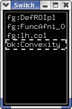
Figure 6: Sample Switch Dset window.
These color planes were used for creating Figure 7 H.
viii. Load Dset:
Load a new dataset (Dset). Datasets can be of 2 formats:
1- NIML (.niml.dset)
This format is
internal to AFNI/SUMA.
2- 1D (.1D.dset)
Simple ASCII
tabular format supporting numerical values only. Each row i contains Nj data values per node. Since this format has no
header associated with it, it makes some assumption about the data in the
columns. You can choose from 3 options:
(see below for
nomenclature)
- Each column has
Ni values where Ni = N_Node
In this case, it
is assumed that row i has values for node i on
the surface.
- If Ni is not equal to N_Node then SUMA will check to see if column 0 (Col_0) is all integers with values v satisfying: 0 <= v < N_Node . If that is the case then column 0 contains the node indices. The values in row j of Dset are for the node indexed Col_0[j].
In the Sample 1D Dset
shown below, assuming N_Node > 58, SUMA will consider the 1st column to
contain node indices. In that case the values -12.1 and 0.9 are for node 58 on
the surface.
- Lastly, if Col_0 fails the node index test, then SUMA
considers the data in row i to be associated with node i.
If you're confused,
try creating some toy datasets like the one below and load them into SUMA.
Sample 1D Dset
(Call it pickle.1D.dset):
25 22.7
1.2
58 -12.1
0.9
Nomenclature and
conventions:
- N_Node is the
number of nodes forming the surface.
- Indexing always
starts at 0. In the example, value v at row 0, column 1 is v = 22.7 .
- A Dset has Ni
rows and Nj columns. In other terms, Ni is the number of values per node and Nj
is the number of nodes for which data are specified in Dset. Ni = 2, Nj = 3 in
the example.
ix.
Load Col
Load a new color plane (Same as c option).
Color plane files (*.col) are a special version of Dset
files, where each node has its red, green and blue values for data.
d. Dset Mapping Block:
i. The Scale bar:
If you need help for this, please get help somewhere.
ii. The Colormap:
The colormap is actually a surface in disguise and shares
some of the functions of SUMA’s viewers:
Keyboard Controls:
r: record image of colormap.
Ctrl+h: this help
message
Z: Zoom in.
Maximum zoom
in shows 2 colors in the map
z: Zoom out.
Minimum zoom
in shows all colors in the map
Up/Down arrows:
move colormap up/down.
Home: Reset zoom
and translation parameters
Mouse Controls:
None yet, some maybe coming.
iii.
I:
Select Intensity (I)
column. Use this menu to select which column in the dataset (Dset) should be
used for an Intensity (I) measure.
I values are the
ones that get colored by the colormap.
No coloring is done if the 'v' button on the right is turned
off.
I(n) value for the
selected node n is shown in the 'Val'
table of the 'Xhair Info' section on the left.
iv.
v:
View (ON)/Hide Dset node colors.
v.
T:
Select Threshold (T)
column. Use this menu to select which column in the dataset (Dset) should be
used for a Threshold (T)
measure.
T values are the
ones used to determine if a node gets colored based on its I value.
A node n is not
colored if:
T(n)
< Tscale
Or, if '|T|' option below is turned ON.
| T(n) | < Tscale .
Thresholding is not applied when the 'v' button on the right
is turned off.
T(n) for the selected node n is shown in the 'Val' table of the 'Xhair Info' section on the left.
vi.
v:
Apply (ON)/Ignore thresholding
vii.
B:
Select Brightness (B)
column. Use this menu to select which column in the dataset (Dset) should be
used for color Brightness (B) modulation.
B values are the
ones used to control the brightness of a node's color.
Brightness modulation is controlled by ranges in the 'B' cells of the table below.
Brightness modulation is not applied when the 'v' button on
the right is turned off.
B(n) for the selected node n is shown in the 'Val' table of the 'Xhair Info' section on the left.
viii.
v:
View (ON)/Ignore brightness modulation
ix.
Mapping Parameters Table:
Used for setting the clipping ranges. Clipping is only done
for color mapping. Actual data values do not change.
Col. Min:
Minimum clip value. Clips values (v) in the Dset less than Minimum (min):
if v < min then v = min
Col. Max:
Maximum clip value. Clips values
(v) in the Dset larger than Maximum (max):
if v > max then v = max
Row I
Intensity clipping range. Values in the intensity data that are less than Min are colored by the first (bottom) color of the colormap. Values larger than Max are mapped to the top color.
Left click locks ranges from
automatic resetting.
Right click resets values to full
range in data.
Row B1
Brightness modulation clipping
range. Values in the brightness data are clipped to the Min to Max range before
calculating their modulation factor
(see next table row).
Left click locks ranges from
automatic resetting.
Right click resets values to full range in data.
Row B2
Brightness modulation factor range.
Brightness modulation values, after clipping per the values in the row above, are
scaled to fit the range specified here.
Row C
Coordinate bias range. Coordinates
of nodes that are mapped to the colormap can have a bias added to their
coordinates.
Nodes mapped to the first color of
the map receive the minimum bias and nodes mapped to the last color receive the
maximum bias. Nodes not colored, because of thresholding for example, will have
no bias applied.
x.
Col
Switch between color mapping modes.
Int: Interpolate
linearly between colors in colormap
NN : Use the
nearest color in the colormap.
Dir: Use intensity values as indices into the colormap. In
Dir mode, the intensity clipping range is of no use.
xi.
Bias:
Coordinate bias direction.
-: No bias thank you
x: X coord bias
y:
Y coord bias
z:
Z coord bias
n: bias along node's normal
This option will produce 'Extremely Cool'[1] images.
[1] Chuck E. Weiss (Slow River/Rykodisc) 1999.
xii.
Cmp:
Switch between available color maps. If the number of colormaps is too large for the menu button, right click over the 'Cmp' label and a chooser with a slider bar will appear.
Alternately, as with many of SUMA’s menus, detach the menu
by selecting the dashed line at the top of the menu list. Once detached, the
menu window can be resized so you can access all elements in very long lists.
More help is available via ctrl+h while mouse is over the colormap.
xiii.
New
Load new colormap. Loaded map will replace a pre-existing
one with the same name.
See ScaleToMap -help for details on the format of colormap
file. The formats are described in the section for the option -cmapfile.
A sample colormap would be:
0 0 1
1 1 1
1 0 0
saved into a cmap file called cmap_test.1D.cmap
xiv.
|T|:
Toggle Absolute thresholding.
OFF: Mask node color for nodes that
have:
T(n) < Tscale
ON:
Mask node color for nodes that have:
| T(n) | <
Tscale
where:
Tscale is the value set by the
threshold scale.
T(n) is the node value in the selected
threshold column (T).
T(n) value is seen in the second cell of
the 'Value' table on the left side.
xv.
sym I:
Toggle Intensity range symmetry about 0.
ON : Intensity clipping range is forced to go from -val to val . This allows you to mimic AFNI's ranging mode.
OFF: Intensity clipping range can
be set to your liking.
xvi.
shw 0:
Toggle color masking of nodes with intensity = 0
ON : 0 intensities are mapped to
the colormap as any other values.
OFF: 0 intensities are masked, a la
AFNI
e.
Data Range
Full range of values in Dset.
Minimum value in Dset column.
Node index at minimum. Right click
in cell to have crosshair jump to node's index. Same as 'ctrl+j' or an entry in
the 'Node' cell under Xhair Info block.
Maximum value in Dset column.
Node index at maximum. Right click in cell to have crosshair jump to node's index. Same as 'ctrl+j' or an entry in the 'Node' cell under Xhair Info block.
Row I
Range of values in intensity (I) column.
Row T
Range of values in threshold (T) column.
Row B
Range of values in brightness (B) column.
E. Viewer Controller
Nothing to write home about yet.
F. Color Planes:
SUMA can display multiple colorized data sets through the use of color planes. For example, the node colors representing brain function that are sent by AFNI form one such plane. You can also envision adding another color plane that delineates different anatomical regions or various drawn ROIS etc. For displaying the results on the surface, all color planes are mixed together based on their stacking order and opacity. It helps to think of each color plane as a colored transparency sheet and the mixing process as a stacking of the various sheets per their stacking order.
There remains one additional complication to this concept. Color planes are divided into two groups: foreground and background. Background and foreground colors are mixed separately then the resultant foreground plane is laid atop its background counterpart. Finally, foreground colors are attenuated by the average intensity of the background color. This attenuation can be turned off with the ‘a’ option.
The following figure illustrates the color plane concepts:
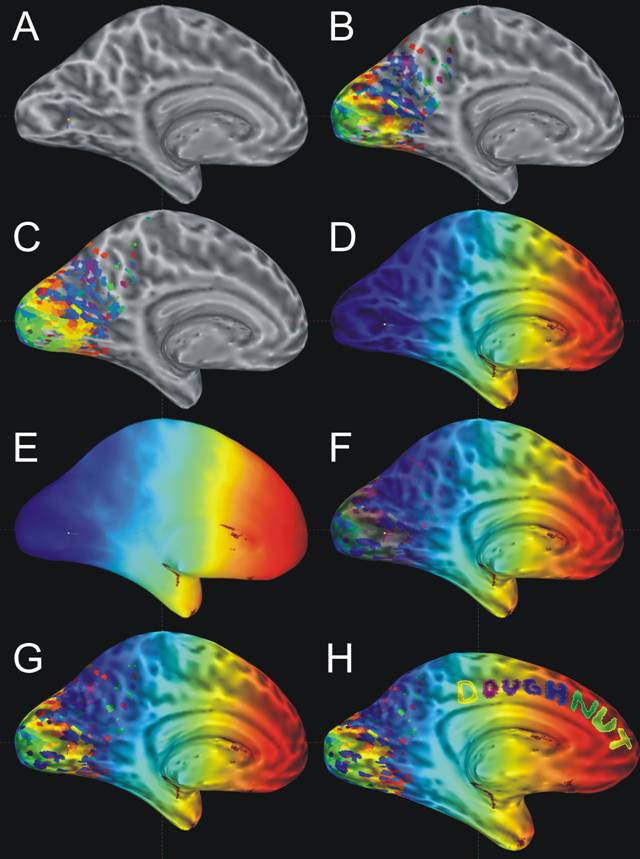
Figure 7: Illustration of color planes
A: Background colors only. The background stack has only one color plane, convexity, in it.
B: Background + 1 Foreground. The foreground stack also has one color plane, FuncAfni_0, in it. This color plane was sent by AFNI and represents the mapping of FMRI data onto the surface. Note how the sulcal patterns (illustrated by the convexity color plane) still show through the foreground colors.
C: Background + 1 Foreground without background attenuation. The foreground colors now completely mask the background colors wherever there is overlap.
D: Background + multiple Foreground. The foreground stack now has two planes in it. The FuncAfni_0 and a new one, lh.col, read in with the ‘c’ option. By default the new color plane is placed on the top of the stack with an opacity of 1 (fully opaque). Therefore the FuncAfni_0 plane is completely obscured. The background attenuation still allows you to find the sulcal highlights.
E: Just like D with no background attenuation
F & G: Just like D with translucent top plane. To allow the FuncAfni_0 color plane to show through, we reduced the opacity of lh.col to 0.5 (F) and 0.0 (G), respectively.
H: Just like D with translucent lh.col and a bunch of drawn ROIs. ROIs are grouped in a separate color plane called DefROIpl (Default ROI Plane).
G. Drawing ROIs:
You can draw Regions Of Interest (ROIs) directly on the surface models. To do so, you must first open the Draw ROI GUI with ‘Ctrl+d’ or Tools --> Draw ROI. An ROI can be a single node, a curve (formed by connected nodes), a loop (or a closed curve or contour) and a filled loop. We begin with a small demo followed by a description of the GUI.
1. Demo:
- In the Surface Viewer window, open the DrawROI GUI with ‘Ctrl+d’.
- When you first open the DrawROI controller SUMA will be in Draw Mode. This is indicated by the cursor’s shape changing from arrow to concentric circles. In drawing mode, you draw with the node picking (typically mouse button 3, or the right mouse button) button. For node picking, you will need to use Shift+Right Click (SRC). To return to normal cursor and mouse functions, toggle Draw Mode off.
- You can also draw in Pen mode by using the Pen toggle button. In Pen mode, the cursor changes into pen and the node picking button becomes the first (left) mouse button no matter what you chose for default node picking button. This makes the drawing interface consistent with AFNI’s ROI drawing. Pen button is only available when SUMA is in Draw Mode.
- Set the Label of this ROI in the GUI to say Test1
- You can draw a segment from the starting node to a new location by moving the mouse and clicking at a new location. Note that the segment will not look like a straight line on the surface. The path drawn on the surface is formed by the intersection of a plane passing through the two nodes.
- You can also draw by holding the shift key and the right mouse button down while moving the mouse. On all but the MAC platforms (will fix that someday, I promise) a green trace follows the pointer. The path along the surface is determined when you release the mouse button.
- NOTE: Sometimes, it is not possible to determine the path along the surface. You will be notified of that and asked to continue from where the algorithm left off. This happens when your paths require a lot of traveling over deep hidden (not visible from the drawing angle) surface regions.
- Draw a few more segments, if that moves you and then close the path with the Join button. You’ll notice the color of the small spheres, used to highlight the nodes in the paths change color.
- Now we’ll fill this closed path by a clicking inside the contour. Filling is done from the starting point (where you clicked) to the contours of the ROI you are drawing at the moment. You may have to do repeated fills if you are of the kind that draws figure eight patterns in a demo.
- The fill (and drawing color in general) is controlled by the value of the ROI and the chosen ROI colormap. Change this value using the Value field and watch the colors change.
- You can try the Undo and Redo buttons at this point which can move you up and down the action stack. Note that Join and Finish are considered as actions and are in the action stack.
- When done and satisfied with the ROI, declare it finished with the Finish button. The spheres highlighting the ROI’s contour disappear. You cannot change the value or the label of a finished ROI.
- If you start drawing again, a new ROI will be automatically created. Create one or two more, just for the fun of it. Remember ROIs can be formed of one node or one trace; they do not have to form a closed loop. Just hit the Finish button when you’re done.
- Once you’ve created a bunch of ROIs, you can switch back and forth between them using Switch ROI. You can delete the current ROI using the delete ROI button and you can load ROIs from disk using the Load button (wait till you save some first).
- You can also save ROIs to disk. To do so, set options after the Save button to NIML and ALL. This will save all the ROIs on the surface to a NIML formatted data set (More info here). These ROIs can be transformed to a surface domain data set using the program ROI2dataset and then transformed into a Volume ROI using the program 3dSurf2Vol.

Figure 8: Draw ROI GUI
2. Usage:
a. Parent: Label of the surface on which the ROI is drawn.
b. Draw Mode: Toggles drawing mode.
If turned on, then drawing is enabled and the cursor changes to a target. To draw, use the right mouse button. If you want to pick a node without causing a drawing action, use shift+right button.
c. Pen: Toggles pen drawing mode
If turned on, the cursor changes shape to a pen. In the pen
mode, drawing is done with button 1. This is for coherence with AFNI’s pen drawing
mode, which is meant to work pleasantly with a stylus directly on the screen.
In pen mode, you draw with the left mouse button and move the surface with the
right button. To pick a node, use shift+left button. Pen mode only works when
Draw Mode is enabled.
d. Afni Link: If turned on, then ROIs drawn on the surface are sent to AFNI.
Surface ROIs that are sent to AFNI are turned into volume ROIs (VOIs) on the fly and displayed in a functional volume with the same colormap used in SUMA. The mapping from the surface domain (ROI) to the volume domain (VOI) is done by intersection of the first with the latter. The volume used for the VOI has the same resolution (grid) as the Surface Volume (-sv option) used when launching SUMA. The color map used for ROIs is set by the environment variable SUMA_ROIColorMap.
e. Label: Label of ROI being drawn.
It is very advisable that you use different labels for different ROIs. If you don’t you won’t be able to differentiate between them afterwards.
f. Value: Integer value associated with ROI.
This value controls the color of the ROI per the ROI colormap.
g. Undo: Multiple level undo of drawing actions
h. Redo: Multiple level redo the last drawing action
i. Join: Connect the first node of the ROI to the last node.
This creates an ROI closed contour (curve); it is a necessary step before the filling operation. Joining is done by cutting the surface with a plane formed by the two nodes and the projection of the center of your window.
You could double click at the last node, if you don’t want to use the ‘Join’ button.
j. Finish: Mark ROI as finished.
This allows you to start drawing a new one. Once marked as finished,
an ROI’s label and value can no longer be changed. To do so, you need to ‘Undo’
the finish action.
k. Switch ROI: Allows you to switch between Drawn ROIs.
You’ll suffer if ROIs on topologically isomorphic surfaces share identical labels.
l. Load: Load ROIs from disk files
m. Delete ROI: Delete a drawn ROI.
This operation is not reversible, so you’ll have to click twice.
n. Save: Save ROIs to disk
You’ll need to choose the format and what to save.
Format options are 1D and NIML. The 1D format is the same one used in AFNI. It is an ASCII file with 2 values per line. The first value is a node index, the second is the node’s value. Needless, to say, this format does not support the storage of ROI auxiliary information such as Label and Parent Surface, etc… For that you’ll have to use NIML, which stands for NeuroImaging Mark Up language, developed by R.W. Cox and heavily used in SUMA ß à AFNI communications. NIML is a whole different story which will be documented (if necessary) in the future. Suffice it to say that in NIML format you can store all the auxiliary information about each ROI, unlike with the .1D format.
The second option is for deciding on which ROIs to save. This: saves the current ROI. All: saves all ROIs on surfaces related to the Parent surface of the current ROI.
o. Close: Close Draw ROI window
Current settings are preserved for the next time you reopen this
window.
Mapping Between Surface and Volume Domains:
Mapping between the surface and volume domains is done using the two programs 3dVol2Surf and 3dSurf2Vol. As their names indicate, the first one maps data from the volumetric domain (like FMRI data) to the surface domain and the second maps data from the surface to the volume domain. Before we present the detailed usage of these programs, we will discuss general aspects of the mapping.
3. Mapping from volume to surface domains:
Mapping from the volume to the surface domain involves mapping voxel values to nodes forming the surface. The simplest mapping is done by the intersection of the surface with the voxel grid. Figure 9 illustrates a small portion of the surface (triangular mesh) and volume (voxel grid). The values at voxel Va shown in blue are assigned to all the nodes in the surface domain that are contained in Va (blue circles in blue voxel). One of the problems with this intersection method is that activated voxels that do not directly intersect the surface do not get mapped to it, even though these voxels contain grey matter or are very close to it (keep in mind that EPI data is often somewhat distorted relative to the high-res anatomy). This problem becomes more severe as voxel size becomes smaller.
Here is another way to consider the same problem, say voxel Va is not significantly activated, but neighboring voxels VA,1 and VA,2(in red), that do not directly intersect the surface do show significant activation. In the simple intersection method, none of these voxels would get mapped to the surface.

Figure 9: Surface and volume domains.
The volume domain is illustrated with the volumetric grid of a 4x4x4 mm EPI data set and the surface domain is illustrated with a small section of the mesh forming an anatomically correct model of the cortical surface.
One method for reducing the aforementioned problem consists of using two homotopic and anatomically correct surfaces that represent the inner and outer boundaries of the gray matter. These two boundaries are represented by Sin and Sout in Figure 10, respectively. Each node ni on the surface receives data from all voxels intersecting the segment formed by ni on Sin and its homolog ni on Sout. A few of those segments are illustrated by the dotted lines in Figure 10 below. Essentially, this method performs an intersection between the volumetric domain and all of the gray matter. In practice, you will have to choose the number of subdivisions between nodes on Sin and Sout. Each subdivision is akin to adding a new homotopic surface between Sin and Sout . For the example depicted in Figure 10 no subdivisions appear necessary because voxel size is large compared to the thickness of the gray-matter.
Since each node might receive values from more than one
voxel, you will also have to choose the option for merging these multiple values
into one value. Averaging is the first option that comes to mind.
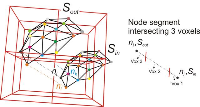
Figure 10: Mapping volumetric data to surface homotopic surfaces.
Nodes with the same ID (index) have matching hues.
3dVol2Surf offers multiple methods for addressing mapping problems; see the program’s help for details.
4. Mapping from surface to volume domain:
Mapping data from the surface domain is less critical than in the other direction because it is usually volumetric data that we want to map to the surface and not vice versa. However, surface to volume mapping has quite a few cool uses such as turning surface-based ROIs to volume based ROIs (or VOIs). ROIs can be manually drawn or automatically generated to delineate functionally (or anatomically) distinct cortical areas. The current implementation 3dSurf2Vol for the surface to volume mapping is essentially the reverse of what was presented above; see the program’s help for details.
H. Surface Models in Talairach Space:
1. Mapping Talairach-Space Volumetric Data:
Talairach-space volumetric data can be mapped onto Talairach-space surface models. This would allow you to map volumetric data onto cortical surface models without having to create surface models for each subject. HOWEVER this is MOSTLY FOR DISPLAY purposes so don’t go analyzing fine topological differences in the patterns of activation for Talairach-space data. The anatomical dataset used as the Talairach template is an average of 27 scans obtained from
MNI http://www.bic.mni.mcgill.ca and UCLA http://www.loni.ucla.edu (Holmes, C.J., Hoge, R., Collins, L., Woods, R., Toga, A.W. and Evans, A.C. 1998 Enhancement of Magnetic Resonance Images Using Registration for Signal Averaging. J. Comp. Asst. Tomograph, 22(2):324-333). Using AFNI, we have created a Talairach version of the N27 brain dataset. Surface models of the N27 data set were created using FreeSurfer (courtesy of Brenna Argall and Patricia Christidis) and transformed into Talairach-space using ConvertSurface. You can download the surface models and the N27 brain from this link: http://afni.nimh.nih.gov/ssc/ziad/SUMA/Talairach_Surface_Models/suma_tlrc.tgz .
To unpack the archive use: tar xvzf suma_tlrc.tgz. The directory ./suma_tlrc should contain find N27_SurfVol+tlrc dataset and a set of left and right hemisphere surfaces.
To view your own Talairach data on the surfaces do the following:
(we'll call TLRC_SURF, the full path to the suma_tlrc directory where the Talairach surface models you have downloaded reside.)
- From TLRC_SURF directory, make a copy of N27_SurfVol+tlrc data set and place it in the directory where you functional data resides (we'll call that directory FUNC_DATA). Example:
3dcopy N27_SurfVol+tlrc FUNC_DATA/Copy_N27_SurfVol
- From FUNC_DATA directory, launch afni with the -niml option
- From FUNC_DATA directory, launch SUMA with the tlrc.spec files and use the copy of N27_SurfVol+tlrc for the surface volume. For example, run from FUNC_DATA directory:
suma -spec TLRC_SURF/ lh.tlrc.spec -sv Copy_N27_SurfVol +tlrc. –dev
NOTE: Functional dataset in Talairach space must be written to disk. Warp-on-demand does not work with SUMA.
- Connect SUMA to AFNI and proceed as usual.
2. Creating Talairach Space Surface Models:
You can transform your surface models to Talairach space as follows:
Ingredients:
SurfIn: A geometrically correct surface model. In any format accepted by SUMA.
SurfVol+orig: The Surface Volume in Original space.
SurfVol+tlrc: SurfVol+orig in Talairach space.
Command Line Sample for FreeSurfer Surfaces:
ConvertSurface –i_fs SurfIn –o_ply SurfIn.tlrc.ply –sv SurfVol+orig –tlrc
For SureFit surfaces, use the –i_sf option instead of –i_fs (see ConvertSurface –help for more info).
Output:
SurfIn.tlrc.ply : Ply format version of SurfIn in Talairach space. The reason the output is in Ply format as opposed to the native format is that SUMA always applies coordinate transformations for surface models in FreeSurfer or SureFit native formats. If you wrote the Talairach-space surfaces back in the FreeSurfer of SureFIt formats (-o_fs or –o_sf, respectively), the surfaces will no longer be aligned with SurfVol+tlrc in SUMA.
To load the Talairach surfaces into SUMA you will need to create a new spec file. The simplest would be to copy a pre-existing one. For example, copy lh.spec to lh-tlrc.spec. You will only need to change the fields of surfaces to which you applied the Talairach transform. In the sample shown below, both smoothwm and pial surfaces were transformed (there is no point in transforming surfaces that are not anatomically correct).
#This is the smoothwm surface in Talairach coordinates.
#This block differs from the one in lh.spec in the following:
# 1- The surface is defined following the field SurfaceName
# instead of FreeSurferSurface. That’s because the surface
# is no longer in the FreeSurfer format.
# 2- The SurfaceType is now Ply
NewSurface
SurfaceFormat
= ASCII
SurfaceType
= Ply
SurfaceName
= lh.smoothwm.tlrc.ply
LocalDomainParent
= SAME
SurfaceState
= smoothwm
EmbedDimension
= 3
#This is the pial surface in Talairach coordinates
#In addition to the changes to SurfaceType and SurfaceName,
#we modified MappingRef to point to lh.smoothwm.tlrc.ply
NewSurface
SurfaceFormat
= ASCII
SurfaceType
= Ply
SurfaceName
= lh.pial.tlrc.ply
LocalDomainParent
= lh.smoothwm.tlrc.ply
SurfaceState
= pial
EmbedDimension
= 3
#For the remaining surfaces, only MappingRef is modified
#to lh.smoothwm.tlrc.ply
NewSurface
SurfaceFormat
= ASCII
SurfaceType
= FreeSurfer
FreeSurferSurface
= lh.sphere.asc
LocalDomainParent
= lh.smoothwm.tlrc.ply
SurfaceState
= sphere
EmbedDimension
= 3
I. Aligning SurfVol to ExpVol:
Aligning the surface volume to the experimental data can be done in different ways. In all cases, the aligned version SurfVol_Alnd_Exp, contains in its header a record of the transformation required to perform the alignment. This same transformation is then used by SUMA to align the surface models with the experimental data. There could be many transformations stored in the header files. For the moment, SUMA only checks for transformations recorded by 3dvolreg and 3dTagalign. In the even that both of these transformations are present, 3dvolreg’s transformation takes precedence.
1. Aligning SurfVol to ExpVol using 3dVolreg:
One convenient way for aligning SurfVol to ExpVol is using the script @SUMA_AlignToExperiment (see Figure 2) which uses 3dvolreg to compute the rotation and translation transform required for alignment. The two data sets require some massaging before using them as input to 3dvolreg which the script does automatically for you.
Alignment via @SUMA_AlignToExperiment is recommended unless it fails to align the two volumes for you. This can happen for a variety of reasons, a few of them are listed below:
- ExpVol and SurfVol are quite different from each other in contrast and/or
voxel size and/or scan coverage. None of the aforementioned parameters
need to be identical between the two scans but sometimes the difference is
too large for 3dvolreg to converge to the correct alignment. The only sure
way to find out is by trying. You can use the sample data used in the
- The EPI data is not in good alignment with ExpVol for a variety of reason. Therefore, it is better to align SurfVol to the EPI data rather than ExpVol. To do so, you’ll need some high-resolution EPI data that still shows anatomical landmarks.
NOTE: If your ExpVol
was acquired with surface coils, you need to correct image intensity
non-uniformity before running @SUMA_AlignToExperiment this can be done with
AFNI’s 3dUniformize.
2. Aligning SurfVol to ExpVol using 3dTagalign:
If alignment of SurfVol to ExpVol via @SUMA_AlignToExperiment script fails, you can use 3dTagalign instead. With 3dTagalign the alignment is performed by matching manually set tags at corresponding locations in the two data sets.
This method has been used for aligning SurfVol to an ExpVol which was a high-res EPI rather than high-res T1 weighted images (by Michael Beauchamp and Brenna Argall).
NOTE: If ExpVol is not in AFNI format (.HEAD and .BRIK) you must create an AFNI format version of it (and often of the functional datasets too). You should also make sure that your functional data is also in good register with the new ExpVol. Info for creating a AFNI-format copy of FSL(http://www.fmrib.ox.ac.uk/fsl/index.html) data is available here. From this point on, we assume that ExpVol is in AFNI format and is in good alignment with your functional data. You can (and should) always check for these alignments with AFNI using the functional overlay and/or opening multiple locked controllers.
Ingredients:
- Vanilla kind SurfVol+orig, the data set created by the @SUMA_Make_Spec_* scripts.
- ExpVol+orig is now a slab of high-resolution EPI data. It shows some anatomy but bares little resemblance to SurfVol in contrast and coverage.
Recipe:
- Use AFNI’s Edit Tagset plugin (DefineDatamode --> Plugins --> Edit Tagset ) and mark the same landmarks in both SurfVol+orig and ExpVol+orig (Brenna used 6 different Tags, the more the better…). PS: I find the “Beep” button to be very useful in determining which tags to use.
We (mortals) can only open one copy of the same plugin per afni session. This means you can’t add tags to the two datasets simultaneously, even though you can view them at the same time (using 2 controllers). I found it useful to run two separate AFNI sessions (run afni twice on command line) which allowed me to open two Edit Tagset plugins simultaneously.
- Run 3dTagalign to align, based on the selected tags, the SurfVol dataset to ExpVol:
3dTagalign -master ExpVol+orig –affine -prefix SurfVol_Alnd_Exp SurfVol+orig
- Now use SurfVol_Alnd_Exp+orig as your anatomical underlay in AFNI and the dataset for SUMA’s –sv option.
J. Creating AFNI datasets from other formats:
1. FSL-ANALYZE to AFNI:
AFNI is able to directly read and display FSL-generated anatomical data and functional data overlaid on top of it. Since FSL data is in ANALYZE format, it seems logical that using the programs 3dANALYZEtoAFNI to transform anatomy and function data to AFNI format should also work for examining the results in AFNI and other related programs. This is not the case however because of the transformation matrices (.mat files) used by FSL to transform datasets into the various coordinate systems: EPI, Highres, and standard. Unlike AFNI, 3dANALYZEtoAFNI does not use these transformations so you’ll have to use 3dWarp instead.
Here is how you can transform Highres and EPI data from FSL
format to AFNI format (requires AFNI version 2.55c
- 3dcopy highres.hdr ExpVol
This creates a high-resolution anatomical volume in AFNI format
- 3dWarp –matvec_in2out example_func2highres.mat –fsl_matvec –gridset ExpVol+orig –prefix Func2 stats/zstat2.hdr
This creates a functional dataset aligned with ExpVol+orig.
· -matvec_in2out option specifies the .mat file containing the FSL transformation matrix needed to align the functional data to the highres data.
· -fsl_matvec option indicates that the transformation matrix is in FSL’s coordinate system (‘LPI’)
· -gridset option specifies which dataset’s grid to use for the output dataset.
· I chose for this example the zstat2.hdr dataset which resides in the FSL directory ./stats
· If you do not want to interpolate your functional data, use the –NN option for nearest neighbor interpolation.
- Make sure that ExpVol+orig and Func2+orig are in good alignment with each other.
DO CHECK TO MAKE SURE ANATOMICAL AND FUNCTIONAL DATA ARE PROPERLY ALIGNED IN AFNI.
K. Surface-Based Cross-Subject Analysis:
In volume-based as well as surface-based cross-subject analysis typically requires two processing steps prior to performing group statistics:
1- Reduce anatomical variability (Talairach transform in the volumetric space)
2- Define the data on a common grid (Standard volume size and a common voxel resolution in volumetric space)
a. This allows for a voxel to voxel correspondence across volumes from different subjects
On surface models, the equivalent of the first step which is currently adopted by Caret and FreeSurfer, consists of warping of the spherical representation of the cortical surface to a template. For the second step, we developed a method for recreating the original surface models using a standard mesh. This allows for node to node correspondence across surfaces from different subjects. As a result, you can use almost all of AFNI’s 3dsomething programs to perform surface-based group analysis.
1. Creating Standard Meshes
Figure 11 illustrates the process of creating a standard-mesh version of an individual subject’s anatomically correct surface model (Anat). The first step, illustrated in Figure 11-A, consists of warping Anat to fit a spherical surface template (Template). Anat is first inflated to a sphere (Sph) and then warped (Warp) so that its sulcal patterns match those of the spherical surface template (Template). For reference, the central sulcus is colored in all surfaces. The warping in this study was carried out using the spherical warping methods from FreeSurfer package; however, the concept is applicable to any surface based warping to a template surface.
The warped spherical surface (Warp) has the same nodes and triangulation (same topology) as Anat and Sph but with different node coordinates (different geometry). Despite the similar appearances of warped surfaces from different subjects, direct comparison of functional activation maps remains cumbersome. Since functional maps are defined on surface nodes, interpolation is again needed to port maps from one subject to another. To eliminate this problem, we instead use the warped surface to create standard-mesh surfaces (SphStd and AnatStd) identical in geometry to Sph and Anat but having a standard topology that would be common across surfaces. On such standard meshes, functional data mapped to node n on one subject can be directly compared to data mapped to node n on another subject’s surface.
To create the standard-mesh surfaces, we start with a triangulated icosahedron (IcoStd, Figure 11 -B, left) with Nstd nodes and whose co-centered sphere has a radius equal to that of Warp. Each node n of IcoStd, projected radially onto Warp, falls inside a triangle T of Warp’s mesh (Figure 11-B, right). Let f(.) be a function defined at each node of the Warp surface. The value of f(.) at node n in the IcoStd surface is computed by interpolation as in Equation 1:
f(n) = a1 f (n1) + a2 f(n2) + a3 f(n3) [1]
where aj is the area (or barycentric) coordinate of node j of T and n1, n2, n3 are the nodes forming T. The left part of Figure 11-C is a graphical representation of the area coordinates of node n inside T. For example, a1 is the ratio of the area formed by triangle n, n2, n3 (cross hatching) to the area of T. The use of area coordinates as weights satisfies the continuity condition across the boundaries of T. For example, as node n approaches edge [n2 n3], the contribution of n1 is reduced to 0. Also, if n approaches n2, the weight for n1 and n3 are reduced to 0.
Rather than interpolate functional MRI data or statistics, we repeatedly replace f(.) in Eq. 1 by the x(.), y(.) and z(.) coordinates of the Anat surface. In other words, the coordinates of node n in AnatStd are obtained by interpolating the coordinates of nodes n1, n2, and n3 in Anat as shown in Figure 11-C. Standard-mesh versions of all other surface models are similarly created. All mapping of functional activity can now be performed on the standard-mesh, anatomically correct surface models instead of the original ones, as described in section Mapping Between Surface and Volume Domains and in Figure 2.
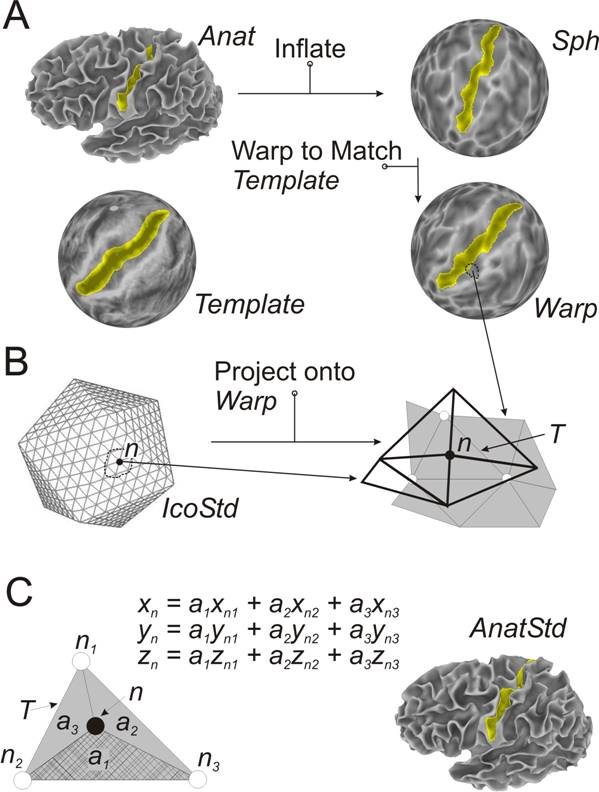
Figure 11: Flowchart for creating standard-mesh surface models.
Sample data were created using FreeSurfer.
The program MapIcosahedron,
written by Brenna Argall, creates the standard-mesh versions of the original
surfaces. The whole process takes about 6 minutes on a 1.2Ghz computer.
The standard-mesh and the original surfaces are almost identical in geometry.
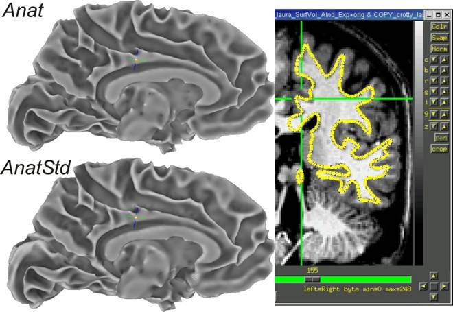
Figure 12: Comparison of original and standard-mesh models.
Original (top left) and standard-mesh surface models
(bottom left) and their intersection with the anatomical volume (right).
Contours of the intersection of the volume with the surface are in blue and
yellow although only the yellow color is visible because of the nearly complete
geometric overlap of the two surfaces.
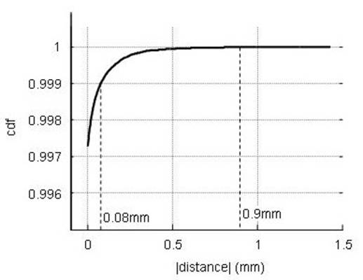
Figure 13: Difference between original and standard-mesh surfaces.
Cumulative distribution
function of the distances between original and standard-mesh surfaces. Mean
distance was 2x10⁻⁵mm; 99.5% of the nodes on the standard meshes
were within 7x10⁻⁴ mm of the original surface. The dotted lines on
the cdf show the maximum distance for the 99.9 and 99.999 percentile levels of
the distances, which were below 0.08 and 0.9 mm, respectively. Graph shows results combined across 6
surfaces.
At time, some nodes (a couple) are considerably off (~15mm) from the original surface. In our experience, this was caused by errors in the topology of the warped sphere. Such errors can be detected using the option –sph_check and –sphreg_check of MapIcosahedron. You will have to correct the original spherical models before proceeding.
With standard meshes, node indices can be directly related to cortical anatomical regions, much as the way mm coordinates are in the Talairach space. In other terms, the same node index from one subject refers to the same anatomical location (within the accuracy of the warping process) as the node with the same index in another subject. This allows for direct anatomical localization and functional data comparison on anatomically correct surfaces without having to further resort to the warping information onto the template spherical brain surface or interpolation along the surface. Figure 14 illustrates this functionality. Standard-mesh versions of the original surface models are shown for six subjects. The colors represent a node’s index in the standard mesh. Regions of similar colors represent similar anatomical locations, despite variability in subject anatomy. For example, note the correspondence of posterior and anterior banks of the central sulcus (orange and green, respectively) and the similar patterns of blue shading in the temporal cortex.
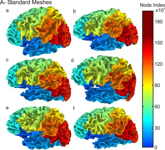
Figure 14: 6 standard-mesh surface models from different subjects.
Set of 6 standard-mesh surface models from different
subjects. Node colors encode for node index n
on the standard mesh. Note how nodes with similar indices correspond to
comparable sulcal landmarks despite the marked anatomical variability across
subjects.
The data shown in Figure 14 can be downloaded and viewed in SUMA from this link. Instructions for viewing the data are in the Readme file accompanying the data. To allow index-based linking across the six surfaces, we made all surfaces have the same Mapping Reference surface. This results in incorrect sulcal shading which is common across all surfaces sharing the same Mapping Reference. This trick and its concomitant artifact will no longer be necessary in the near future. Stay tuned.
2. Statistical Analysis On The Surfaces
The statistical analysis in this example is a caricature intended to illustrate the process of data handling.
•
Use 3dVol2Surf to map individual subject data onto each standard-mesh
surface
–
Example: Mapping functional data onto surface, with
thresholding
3dVol2Surf \
-spec lh.spec \
-surf_A lh.smoothwm.asc \
-surf_B lh.pial.asc \
-sv SurfVol_AlndExp+orig \
-grid_parent
DataVol+orig \
-cmask '-a DataVol+orig[3] -expr step(a-72)' \
-map_func
ave \
-oom_value -999.9 \
-out_1D DataSurf.1D.dat
Written by Rick Reynolds
•
-spec: SUMA spec file containing surface(s) to
be used in mapping.
•
-surf_
: Specify the surface(s) to be used by the mapping
3dVol2Surf uses one or two surfaces for the mapping.
•
-sv: Surface Volume used to align surface to data
•
-grid_parent: AFNI volume containing data to be mapped.
DataVol contains 4 sub-bricks with the last one being the threshold.
•
-cmask: Option for masking data in DataVol. Threshold
value was 72
•
-map_func: Method for handling multiple voxel to one
node mapping
•
-oom_value -999.9 : Assign -999.9 to nodes that fall in
inactivated voxels
•
-out_1D: Output file
– Use –help option for detailed help (>500 lines)
–
See 1D files as data sets
for more help on output
•
Sample Output, the 1D format
#
--------------------------------------------------
#
surface 'lh_mappedSmWm.asc', 'ave' :
#
# node
1dindex i j
k vals v0
# ------
------- --- ---
--- ---- --------
3
31978 42 51
7 2 -18.80515
64
30633 41 30
7 1 13.49998
7255
43375 47 37
10 2 11.25401
7256
43375 47 37
10 1 11.70573
7257
43375 47 37
10 2 11.25401
7317
39144 40 35
9 2 14.67585
7318
39145 41 35
9 2 17.08102
7358
47406 46 36
11 1 15.62297
7359
47406 46 36
11 1
15.62297
7435
30633 41 30
7 1 13.49998
(I omitted from the table above all
nodes that had no values mapped to them. Such nodes will have v0 = -999.9 )
•
Node: Surface node index
•
1dindex: AFNI 1D Index of voxel mapped to node. In
cases where multiple voxels contribute to 1 node, the first voxel is listed
•
i, j, k: AFNI indices of voxel mapped to node (3D
version of 1dindex)
• vals: Number of voxels mapped to node v0: Value mapped to node. Here we mapped values from one sub-brick. If you map N sub-bricks you'll have v0 .. VN-1 columns.
•
ScaleToMap is used to colorized the mapped data for
later display in SUMA
ScaleToMap -input
DataSurf.1D.dat 0 6 \
-cmap RGYBR20 \
-msk -998 -1000 \
> DataSurf.1D.col
•
-input DataFile icol vcol: Node data file followed by
column indices for node index and data
•
-cmap MapType: Type of colormap
•
-msk msk0 msk1: Range of values to exclude from color
map
•
> DataSurf.1D.col : redirection of output to file
(screen is the default). Output contains 4 columns: node index, R, G, B
•
DataSurf.1D.col can be loaded into SUMA using 'c'
option
# index R G B
3 0.000 0.862127
0.137873
64 1.000000 0.800135
0.000000
7255 1.000000
0.943492 0.000000
7256 1.000000
0.914660 0.000000
• Finally, calculate some group-statistic: the mean value at each node from 3 subjects:
1deval
-a 'DataSurf_s1.1D.dat[6]' \
-b
'DataSurf_s2.1D.dat[6]' \
-c
'DataSurf_s3.1D.dat[6]' \
-expr '(a + b + c) / 3' \
-index 'DataSurf_s1.1D.dat[0]' \
> DataSurf_mean.1D.dat
1deval works much like 3dcalc but
with 1D files
-index option allows the addition
of an index column (node indices) to the output.
DataSurf_mean.1D.dat will contain 2 columns: node index and mean value
•
Appreciate why we forced an output for all node indices
•
Things to be careful about:
–
1D files do not explicitly encode domain information
•
It is up to you to make sure that the i th entry
in all 1D files corresponds to the same node.
•
You must have the same number of values in all files
•
Things to think about:
•
When mapping data from volume to surface domains
–
If mapping assigns multiple voxels to one node
•
How do you deal with functional data sets?
–
Do you average statistics?
–
Do you apply a threshold before or after averaging?
»
What if some of the voxels are active and some are not?
•
These problems are best avoided by:
–
Mapping the time series data onto the surface
–
Performing statistical analysis directly in the surface
domain using 3dSomething AFNI
programs
•
When combining surface data across subjects
–
Same concerns as with volumetric group analysis
•
You can also create volumetric data from surface-based
data
–
use 3dSurf2Vol, the reciprocal of 3dVol2Surf
L. Auxillary Programs:
Much as in AFNI, a lot of work can/will be done from the command line using auxiliary programs.
Type ‘suma –progs’ for the latest
list of programs distributed with SUMA
1. 3dSurf2Vol:
This program maps data in the surface domain to the volume domain. You can use this program to do things like:
Change a surface ROI to a VOI
Create a volume mask from the entire surface
Create a volume mask of the region between two surfaces
Map data defined on the surface to the volume
Etc.
For help, consult the output of: 3dSurf2Vol –help . Also see the complimentary program 3dVol2Surf and the section on mapping between
domains.
2. 3dVol2Surf:
This program maps data in the volume domain to the surface domain. It is the opposite of 3dSurf2Vol and shares many of that program’s options. More help from: 3dVol2Surf –help . See also the complimentary program 3dSurf2Vol and the section on mapping between domains.
3. CompareSurfaces:
This program compares the distance at each node in surface 1 (S1) to surface 2 (S2). For each node n1 on S1, the distance to S2 is computed along the local surface at n1. S1 and S2 are the first and second surfaces encountered while loading the spec file specified at the command line. See CompareSurfaces –help for detailed usage information.
4. ConvertSurface:
A program for converting surface files from one format to
another. In addition, the program can be used to apply certain transformations
on the surface coordinates. In particular, you can rewrite a surface model with
its coordinates transformed by the alignment transform in SurfVol_AlndExp.
If you do so, take care not to reload the surface into SUMA with –sv
SurfVol_AlndExp because the transform will then be applied twice. I do not
recommend that you transform the coordinates unless you really know what you
are doing. Also, you can use this program to write out surface models transformed into
Talairach Space.
5. CreateIcosahedron:
A program to create
an Icosahedron (by B. Argall).
6. FS_read_annot:
A program to read FreeSurfer’s surface annotation files into SUMA.
7. inspect:
A program to show the (interpreted) contents of a spec file.
8. MakeColorMap:
A program to
generate colormaps to your liking.
9. MapIcosahedron:
This program creates standard-mesh versions of cortical surface models using the method outlined in Figure 11.
•
Required Data:
–
Original Surface models
–
Warped Spherical surface
–
Spec file of the surfaces above (i.e. lh.spec)
•
Creating the standard-mesh versions of the original
surfaces
MapIcosahedron -spec
lh.spec \
-ld 141 \
-prefix ld141
-spec SpecFile:
option specifying spec file with original surfaces
-ld n : number of subdivisions for each
edge of the icosahedron.
Nv = 2 + 10n2 (198812 vertices)
Nt = 20n2 (397620
triangles)
Ne = 30n2 (596430
edges)
-prefix: prefix
assigned to standard mesh surfaces
•
You can compare original and standard surfaces using:
–
SUMA
•
create a spec file containing both original and
standard-mesh surfaces.
•
open two views, one showing original surface and one
showing standard-mesh surfaces
•
link viewers by coordinates (not by node index) from
the SUMA controller (ctrl+u)
–
CompareSurfaces Written by Shruti Japee
•
a program that
calculates the distance from each node on surface 1 along its normal to surface
2
–
SurfaceMetrics
•
a program that calculates metrics of the mesh like edge
lengths, triangle areas, curvature, etc.
At times, there are localized
distortions between the standard-mesh surface and the original surface. So far,
these have all been caused by topological errors in the original spherical
surfaces. The program SurfQual was
written to highlight these topological errors which, if causing distortions,
must be fixed with the program used to generate them. These topological errors can
be ignored if they do not cause any visible distortions in the standard-mesh
surfaces.
10. quickspec:
A program to quickly generate a spec file for a set of
surfaces.
11. ROI2dataset:
This program is used to turn Drawn ROIs into surface domain data sets. These datasets can be mapped to the volumetric domain using the program 3dSurf2Vol.
If a certain node is a member of more than one ROI, only the first membership is preserved. The program will warn you of such occurrences.
Detailed help is available through the command line: ROI2dataset –help .
12. ScaleToMap:
This program is used to map values to colors based on a specified color map. For example, you can use this program to colorize the results of 3dVol2Surf.
13. SUMA_glxdino:
A simple program to test installation of OpenGL on your computer.
14. SurfMeasures:
A program to output various measures about a surface such as surface area, volume between two isotopic surfaces, and a whole lot more.
15. SurfaceMetrics:
A program to output sets of parameters about the surface’s geometry and topology.
16. SurfSmooth:
A program to filter surface geometry (no shrinkage) and surface-defined data.
17. SurfPatch:
A program to create a surface patch out of a set of node indices
18. SurfQual:
A program to point to locations on a spherical surface where either the geometry or the topology is flawed. These errors on the spherical surfaces might cause localized distortions in the standard meshes created with MapIcosahedron. If that’s the case then you have to correct the errors in the original spherical surfaces using the program that created them.
The errors are very hard to spot without the use of SurfQual. They often occur as twists and folds in the spherical mesh without much geometrical distortion. The figure below is an extreme close up on one of these errors found on the original spherical surface.

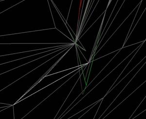
Figure 15: Topological errors in spherical surfaces that might result in local distortions of standard-mesh surfaces.
The figure on the left shows the spherical mesh with the
topological error in the mesh at the center. The figure on the right is a close
up of the error zone from the left.
M. Communication between AFNI and SUMA:
1. Starting NIML connection:
In order for SUMA to communicate with AFNI you need to make sure AFNI is listening for connections. This is done by either using the option -niml when afni is launched or by starting niml from:
>AFNI> Define Datamode --> Misc --> Start niml.
By default, it is assumed that both AFNI and SUMA are running on the same machine, therefore the communication is to and from localhost. But the two programs can be running on separate machines, you just have to tell SUMA where AFNI is running and make sure AFNI accepts connections from SUMA's machine. For example, say we're running SUMA on ell and AFNI on yak.
When running SUMA specify AFNI's hostname using the -ah option:
> suma other options here -ah yak.zoology.net
or
> suma other options here -ah 123.324.223.112
On yak, where you'll be running AFNI you need to add eel as a trusted host by adding the following environment variable (following examples apply to csh users):
> setenv NIML_TRUSTHOST_01 eel.zoology.net
or
> setenv NIML_TRUSTHOST_01 123.324.223.16
or
> setenv NIML_TRUSTHOST_01 123.324 (to accept connections from all addresses
beginning with 123.324)
You can add more trusted hosts by using NIML_TRUSTHOST_02, NIML_TRUSTHOST_03 etc.
For more information on how SUMA and AFNI communicate and on how to have your program communicate with AFNI in a similar manner, check for upcoming documentation on AFNI's webpage.
Bugture: When communicating between linux (SUMA) and SGI (AFNI), the SGI thinks the connection is from 255.255.255.255 which is an illegal address. If that happens to you then use this fix until we sort out the problem:
> setenv NIML_TRUSTHOST_01 255.255.255.255
2. AFNI to SUMA Communication:
- Functional Overlay
AFNI will send the colorized mapping of a functional volumetric dataset to the surfaces intersecting that volume. For this to happen, you’ll need to have the .BRIK part of the functional data set on disk. .HEAD only datasets, which are viewed as “Warp Func on Demand” in AFNI will not get mapped to the surface. “Warp on Demand” is used when you interpolate your functional data to a different resolution or when you only have a .HEAD file defining the dataset. The .BRIK part of such a dataset is created by AFNI on the fly (on demand) by transforming a parent dataset specified in the .HEAD file. This is how Talairach datasets are treated by default in AFNI. To map such datasets to the surface, you will need to write their .BRIK components to disk using the program adwarp or the “Write: Func” button from AFNI’s “Define Datamode” panel.
If you have both .HEAD and .BRIK parts of the dataset on disk and “Warp on Demand” settings in AFNI do not affect the mapping of volumetric functional data to the surface: No .BRIK = No function on surface.
- Crosshair Location
Each new crosshair location is sent to SUMA which may or may not be able to attach it to a particular surface, depending on the crosshair’s coordinates.
3. SUMA to AFNI Communication:
- Crosshair Location
SUMA will set AFNI’s crosshair location based on the coordinates of the selected node in the mapping reference surface.
II. Appendix A:
A. Surface Reconstruction Software:
SUMA currently works with surface models created by
FreeSurfer (http://surfer.nmr.mgh.harvard.edu/)and
SureFit(http://stp.wustl.edu/SureFit/).
We can add other models if provided with sufficient information about file
formats and coordinate spaces.
B. File Formats:
1. 1D files:
1D files are ASCII files for storing a matrix of numbers. You can place comments at the beginning of the file by placing the # character at the beginning of each comment line. The following is an example of a 1D formatted surface domain data set:
# Sample surface domain data set
# 1st column contains the node index
# 2nd – 4th column contain 4 values associated with each node
# these 4 values represent the node’s r g b colors (range 0 – 1)
1324 0.1 0.74 0.2
1528 0.34 0.22 0.54
2314 0.89 0.01 0.21
…
1D files cannot contain auxiliary information describing the data. For example, ROIs saved in 1D format are reduced to a bunch of node indices and node values. No information is kept about their labels, their parent surface, etc. You should use this format sparingly.
2. 1D files as surface data sets:
• Most 3dSomething command line programs can read 1D instead of volumetric data
–
The "spatial" direction is down the columns
(vertical).
–
The default is that across the rows (horizontal) is a
"bucket" dimension.
–
The new environment variable AFNI_1D_TIME, if set to
YES, will cause the horizontal direction to be the time axis (with TR=1).
•
This makes it possible to input .1D files to programs
that process 3D+time datasets
–
files will probably need to be transposed first -- so
that the time axis is horizontal rather than vertical.
1dtranspose fred.1D fred_q.1D
3dFourier -prefix fred_filt_q -highpass
0.1 -retrend fred_q.1D
1dtranspose fred_filt_q.1D fred_filt.1D
rm -f fred_q.1D fred_file_q.1D
• It is possible for 3dVol2Surf to try to output a 1D file that is > 2GB. Such files are too large to be handled by most current operating systems. If you encounter such a problem, the only solution is to do the mapping for a subset of the nodes at a time. Do so by using the options –first_node and –last_node in 3dVol2Surf. The other solution is to output the data in NIML format which can be a lot smaller. However at the moment, only few programs other than can read NIML formatted datasets. Stay tuned for more.
3. NIML files:
NeuroImaging Markup Language (NIML) files can be either in ASCII or binary form. They contain one or more NIML elements. The NIML format was developed by Dr R. W. Cox and is used for data storage and communication between AFNI and SUMA. For detailed information about the NIML format and its API see http://afni.nimh.nih.gov/afni/niml/NIML_base.html.
Briefly, a NIML element contains a set of attributes followed by data. The following is an example of a Drawn ROI element in NIML format written to an ASCII file:
# <Node_ROI
# ni_type = "SUMA_NIML_ROI_DATUM"
# ni_dimen = "6"
# ni_datasize = "128"
# idcode_str =
"XYZ_JpDDDD1yuVsz5hOTlVP53A"
# Parent_idcode_str =
"XYZ_cE3DT7k7uVKaGV2Vy2IS6g"
# Label = "j4"
# iLabel = "4"
# Type = "2"
# ColPlaneName = "DefROIpl"
# FillColor = "1.000000 0.000000 0.000000"
# EdgeColor = "0.000000 0.000000 1.000000"
# EdgeThickness = "0"
# >
1 4 1 324
1 4 2 324 288
1 4 3 388 325 314
1 4 3 314 319 321
1 4 3 321 318 271
3 4 3 271 317 324
4 1 1 315
# </Node_ROI>
NIML ASCII files do not have to have the # character before each attribute but they are more readable in this format. The sample element shown here is far from being the simplest type of element. This element keeps track of the different actions used to create the ROI and thus allows for Undo/Redo actions once an ROI is reloaded into SUMA. In most cases, the data part of the element consists of a matrix of numbers such as in the output of the program ROI2dataset.
4. Spec files:
The Spec file contains information about the surfaces that will be viewed. Information is specified in the format: field = value. The = sign must be preceded and followed by a space character. # delimit comment lines, empty lines and tabs are ignored. In addition to fields, there is also the NewSurface tag, which is used to announce a new surface. Unrecognized text will cause the program parsing Spec file to complain and exit.
The fields are:
a. Group:
Usually the Subject's ID. In the current SUMA version, you can only have one group per spec file. All surfaces read by SUMA must belong to a group.
The following
fields are used to specify the files defining a surface’s geometry and
topology:
b. FreeSurferSurface:
Name of the FreeSurfer surface file containing both geometry and topology. Patch files are also acceptable.
c. SurfaceName:
Name of the file containing surface topology and geometry. Use this field with all but surfaces of the type FreeSurfer, SureFit and 1D.
d. SurfaceVolume:
Name of the surface volume for this surface. This field allows you to assign a different surface volume to different surfaces in the same spec file. Normally, the surface volume specified on command line with the –sv option is used by all surfaces in the spec file.
If you specify a SurfaceVolume for a particular surface in
the spec file, it will override the –sv on command line for that one surface.
e. SureFitTopo:
Name of SureFit’s .topo file containing the topology (mesh)
of the surface.
f. SureFitCoord:
Name of SureFit’s .coord file containing the coordinates of
each node forming the surface.
g. SureFitVolParam:
Name of SureFit’s .params file containing coordinate offset
information (and more).
h. TopoFile:
Name of 1D format file
containing surface topology. Three node indices per line.
i. CoordFile:
Name of 1D format file containing node coordinates. X Y Z coordinates per line.
j. SurfaceFormat:
ASCII or BI. Only ASCII is supported at the moment.
k. SurfaceType:
FreeSurfer (http://surfer.nmr.mgh.harvard.edu/), SureFit (http://stp.wustl.edu/SureFit/) , Ply (http://graphics.stanford.edu/data/3Dscanrep/) or 1D
l. SurfaceState:
Surfaces can be in different states such as inflated, flattened, etc. The label of a state is arbitrary and can be defined by the user. The set of available states must be defined with StateDef at the beginning of the Spec file. Surfaces having the same state are displayed in the same viewer, that is how both left and right hemispheres can be shown simultaneously.
m. StateDef:
Used to define the various states. This must be placed before any of the surfaces are specified. Surface States that are not defined will cause the program parsing the Spec file to complain and quit.
n. LocalDomainParent (LDP):
This field specifies the name of surface that has the
original mesh. Correspondence between surfaces having the same Local Domain Parent
(LDP) is maintained by node indices. Use SAME when the surface itself is the LDP.
The LDP used to be the same as the MappingRef field
which is now obsolete.
Currently, surfaces that have LocalDomainParent = SAME are
sent to AFNI. However, in the very near future, all surfaces that are
anatomically correct will be sent to AFNI.
The default LDP for FreeSurfer surfaces is the smoothed gray
matter/ white matter boundary. For SureFit it is the fiducial surface.
o. MappingRef (Obsolete, see LocalDomainParent):
Name of a surface to be used for mapping functional activity in the volume onto the cortical surface. That's necessary because it makes no sense to map volumetric data directly onto surfaces in certain states. The default for FreeSurfer surfaces is the smoothed gray matter/ white matter boundary. For SureFit it is the fiducial surface. Use SAME when the Mapping Reference for a surface is the surface itself.
p. EmbedDimension:
Embedding Dimension of the surface, 2 for surfaces in the flattened state, 3 for other.
C. Environment variables:
Environment variables can be saved in a .sumarc file (in the user’s home directory) or in the .afnirc. Here’s a link to a sample .sumarc: http://afni.nimh.nih.gov/ssc/ziad/SUMA/Sample-.sumarc-
1. SUMA_ArrowRotAngle:
Angle in degrees for each arrow key rotation.
2. SUMA_ColorPattern:
Some default options for SUMA’s GUI interface. Choose from AFNI, EURO and DEFAULT. Default is actually EURO, DEFAULT is quite hideous.
3. SUMA_SwapButtons_1_3:
Set to YES to swap mouse buttons 1 and 3. Default is NO.
4. SUMA_BackgroundColor:
r,g,b triplet specifying the color of the background. Default is 0,0,0. Use no spacing between the numbers. r,g,b values can range from 0.0 to 1.0.
5. SUMA_ROIColorMap:
Name of colormap to use for ROI drawing. See Colormaps for a complete list.
6. SUMA_NumConvSmooth:
Number of smoothing operations to run on convexity data, default is 5.
7. SUMA_ConvColorMap:
Name of colormap to use for convexity data. Common choices include gray02 or ngray20.
8. SUMA_ConvBrightFactor:
Brightness factor for convexity colors. Default is 0.5.
9. SUMA_NumForeSmoothing:
Number of smoothing operations to run on mixed foreground color pane before mixing with background. Confused? Try smoothing, using keyboard option ‘8’. Note that these operations can significantly slow down the display.
10. SUMA_ColorMixingMode:
Setup the color mixing mode (ORIG (default), MOD1). This affects the way colors add up from different layers.
In ORIG mode:
In MOD1 mode:
11. SUMA_AFNI_TCP_PORT:
Port for communicating with AFNI. Listening ports are derived from SUMA_AFNI_TCP_PORT . (default 53211)
12. SUMA_WarnBeforeClose:
Ask stupid questions when user hits Escape to close a viewer. (NO/YES(default))
13. SUMA_MaskZero:
Mask node values = 0 ? (YES (default)/NO)
14. SUMA_AbsThreshold:
Threshold if Val < thr (NO) or | Val | < Thr (YES(default))
D. Colormaps:
SUMA has a set of pre-defined colormaps (cmaps).
Cmaps starting with the name ‘afni_’ are AFNI’s default colormaps. For example, afni_n5 would be AFNI’s 5 color negative range colormap. Cmap afni_p20 would be AFNI’s 20 color map with the positive range. Available AFNI cmaps are:
afni_n2 … afni_n20 and afni_p2 … afni_p20.
The following cmaps are also available:
roi128, roi64, bgyr64, byr19, bgyr19, bw20, gray20, grayi02, gray02, ngray20, rgybr20.
You can look at these maps using SUMA’s surface controller. You can also create your own colormaps as specified in the help for option –cmapfile in program ScaleToMap.
III. Glossary
A. .afnirc:
The .afnirc file is used to setup certain environment variables. Here's a link to mine http://afni.nimh.nih.gov/ssc/ziad/SUMA/Sample-.afnirc- to use it you should place it in your home directory and save it as .afnirc . I use it to specify environment variables, layout of windows when afni is launched (to modify the layout use Define Datamode --> Misc --> Save Layout) and to specify a colormap.
B. @SUMA_AlignToExperiment:
A csh script used to align the Surface Volume SurfVol to the Experiment's Volume ExpVol . The script requires programs present in AFNI's distribution. For more information, run:
> @SUMA_AlignToExperiment -help
C. @SUMA_Make_Spec_FS
A csh
script used to create the Spec file of surface models created by FreeSurfer.
The script requires FreeSurfer's mris_convert and afni's to3d programs. For
more help, run:
>
@SUMA_Make_Spec_FS -help
D. @SUMA_Make_Spec_SF
A csh
script used to create the Spec file of surface models created by SureFit. The
script requires no special programs but will check for afni and suma and will
warn you if they do not exist. For more help, run:
>
@SUMA_Make_Spec_SF -help
E. Anatomically Correct Surfaces:
Surface models whose geometry models an aspect of the cortex
are called anatomically correct. Such surfaces include representations of the
gray/white matter or gray/CSF or mid-gray matter boundaries. Anatomically
incorrect surfaces include inflated, flattened and spherical representations of
the surfaces.
F. Axis Order:
A three character string indicating the orientation of the
set of images used to create a 3d volume. For example, LSP means that the
orientation is from Left to Right along the X axis,
G. Colormap generation:
The program MakeColorMap (installed with suma) can generate a colormap to your liking. For more information:
> MakeColorMap
H. Dsets (Surface Data Sets):
Data defined over the surface nodes are referred to as Dsets in SUMA. Dsets can be stored in 1D
format (most common at the moment) and later in NIML format. See here for more info.
I. Experiment anatomy Volume (ExpVol):
With every new experiment, you need to collect a high resolution anatomical data set covering the entire brain. This data set is commonly used as an underlay for functional data collected during the same experimental session. The ExpVol used in SUMA_demo was obtained at 3T with FSPGR pulse sequence and a resolution of 0.975x0.975x1.2 mm. This scan took 3 minutes to acquire. Since SurfVol will be aligned to ExpVol, the coverage and contrast of the two should be comparable. ExpVol's Image quality does not have to be as good as SurfVol's (see example in Demo Data), just good enough for the alignment to succeed. You can use the aligned version of SurfVol for all your displays.
J. Facet:
A triangular element that is part of the mesh defining the surface (called FaceSet in SUMA's code). A Facet is defined by three nodes and their connections.
K. Homotopic or Topologically Isomorphic Surfaces:
Surfaces that share the same topology (mesh). For example
the pial and inflated surfaces are homotopic. While the term homotopic is
correct, short and convenient to use, we will often use “Topologically
Isomorphic” instead to appear more sophisticated and impress the largest number
of people.
L. IDcode:
The ID code is a unique identifier string that is assigned
to various objects in AFNI and SUMA. In particular, data sets have IDs attached
to them (just like AFNI’s data sets). No two objects should ever, ever, have
the same ID.
M. Mapping Reference Surface (MapRef):
Deformed surfaces (such as inflated or flattened) cannot be directly used to map functional data onto them. The mapping is done onto the Mapping Reference Surface then transferred onto the deformed surface. The link to AFNI is done via the MapRef surface.
N. Node Datasets (Dsets):
Same as Surface
Domain Datasets.
O. Node Index or Node ID:
Nodes are identified by their indices and the surfaces they belong to. Node indices are between 0 and N_Node-1 where N_Node represents the largest number of nodes making up a surface. Nodes in different surfaces of the same group share the same node indices although nodes may have different coordinates.
P. Nodes:
Surfaces are defined by nodes (vertices) that form a triangular mesh. The mapping of function is performed onto the nodes.
Q. Shell:
“A utility program that enables the user to interact with
the UNIX operating system. Commands entered by the user are passed by the shell
to the operating system which carries them out. The results are then passed
back by the shell and displayed on the user's display.” (Definition from http://www.mcsr.olemiss.edu/unixhelp/glossary/gs.html
)
It's that usually black window that some love to hate where one types unix commands. (Definition from Hell)
R. SRC:
Shorthand for: Shift key + Right Click mouse
S. Surface anatomy Volume (SurfVol):
The surface model is created from a high-resolution anatomical scan referred to as Surface Antomical Volume (SurfVol). For FreeSurfer surfaces, this volume is created by the script @SUMA_Make_Spec_FS. For SureFit surfaces, this volume is a 1x1x1mm AFNI brick in LPI orientation. See 3dresample example for more info. The data used to create SurfVol was obtained by averaging 4 scans obtained at 3T using MPRAGE pulse sequence (more scanning params). The scanning took 4x9 minutes but is only needed once per subject. Data set was resampled to 1x1x1 for FreeSurfer's and SureFit's use.
T. SurfVol, Aligned to Experiment (SurfVol_AlndExp):
This is the version of SurfVol that has been aligned to ExpVol (the new experiment’s high resolution anatomy, see Figure 2 and this script). The header of SurfVol_AlndExp contains an affine transform which is a record of the transformation needed to align SurfVol with ExpVol. That matrix is stored in the field VOLREG_MATVEC if you used @SUMA_AlignToExperiment script or in TAGALIGN_MATVEC if you used 3dTagalign to align SurfVol to ExpVol. If any of VOLREG_MATVEC or TAGALIGN_MATVEC transforms are encountered, they are applied to the coordinates of the surface models read into SUMA which should bring the surface models in alignment with the functional data.
NOTE: Actually, there are additional coordinate transformations done for SureFit and FreeSurfer surfaces before the transform find in SurfVol_AlndExp.
U. Surface Domain:
The surface domain is the mesh (grid) formed by
interconnected nodes which define the surface. Both the geometry (spatial
location of the nodes) and the topology (connectivity between the nodes) define
a domain. Data defined in the surface domain are attached to (or defined at)
the nodes forming the surface. See also
Volume Domain.
V. Surface Domain Datasets (Dsets):
These are data sets defined over the domain of the surface. These data sets form matrices with one column representing the node index (ni, a.k.a node id) followed by p values (i_val. 1 … i_val. p) associated with each node. Those p values can potentially be any assortment of parameters, though some dataset formats will be limited. In some instances, the node index column may be missing and the node’s index is assumed to be equal to the row index.
… …
ni i_val.
1 i_val. 2 … … i_val. p
nj j_val. 1 j_val.
2 … … j_val. p
… …
Note that unlike its volumetric counterpart, the domain is not implicitly defined in the dataset. Consequently, such a dataset alone cannot be visualized without specifying its surface domain (location and connectivity of the nodes). Surface domain datasets are also called node datasets.
A colorized dataset is called a color plane.
a. Sample dataset output by ROI2dataset:
The first column of numbers represents the node indices the second contains an index identifying the ROI. Lines starting with # denote comments. The file is in the AFNI 1D format although this example can also double as a NIML dataset.
# <Node_ROI
# ni_type = "2*int"
# ni_dimen = "105"
# ni_datasize = "420"
# idcode =
"XYZ_MpBElNAbBjPM00K3RCordQ"
# DomParent_idcode =
"XYZ_cE3DT7k7uVKaGV2Vy2IS6g"
# GeomParent_idcode
# TypeCol_0 = "Node_Index"
# AttrCol_0
# TypeCol_1 = "Node_Index_Label"
# AttrCol_1
# History = "ROI2dataset : ROI2dataset
-prefix test -of 1D -input r5.niml.roi j1.niml.roi j2.niml.roi j3.niml.roi
j4.niml.roi vrf.niml.roi vr.1D.roi vr.niml.roi test.niml.roi"
# >
2 3
258 1
268 1
269 0
270 0
271 1
272 2
273 2
274 1
275 1
276 1
277 0
278 1
279 1
...
451 0
452 1
# </Node_ROI>
W. Surface State :
Surface models exist in various states of deformation such as white/gray matter boundary, pial surface, inflated, flat, etc. The State of a viewer is the same as that of the surfaces displayed.
X. Volume Domain:
The volume
domain is the 3 dimensional voxel grid set by the volume’s location in space
and resolution. Data defined in the volume domain is attached to voxels forming
the volume. See also Surface Domain.
IV. Troubleshooting:
This is
supposed to contain notes on bugs extraneous to AFNI/SUMA that we cannot fix.
For everyday help, use the AFNI message board: http://afni.nimh.nih.gov/afni/community/board/list.php?f=1
You can
also contact the authors if necessary but the response, unless of a private
nature, will end up posted on the message board anyway.
Ziad S.
Saad: ziad@nih.gov
Rick C.
Reynolds: rickr@nih.gov
A. X server crash with 'w' option:
FORGET
ABOUT ‘w’, use ‘r’
or ‘R’ instead.
This
option has caused the X server to crash on a computer running linux redhat 7.2
with an ASUS V7700 GeForce2 graphics card. The crash is caused when one
attempts to render to a pixmap. We reinstalled mesa and updated nVIDIA's
kernels but the problem was not fixed. Changing the graphics card fixed the
problem.
V. Figure List:
Figure 1: Aligning the surface to experimental
data.
Figure 2: Mapping volumetric data onto surface
Figure 3: Detail of cross-hair
Figure 5: Surface controller GUI
Figure 6: Sample Switch Color Plane window.
Figure 7: Illustration of color planes
Figure 9: Surface and volume domains.
Figure 10: Mapping volumetric data to surface
homotopic surfaces.
Figure 11: Flowchart for creating
standard-mesh surface models.
Figure 12: Comparison of original and
standard-mesh models.
Figure 13: Difference between original and
standard-mesh surfaces.
Figure 14: 6 standard-mesh surface models from
different subjects.
VI. Table of Contents
1. Surface rendering with direct AFNI link:
4. Simultaneous left / right hemisphere
display:
5. Talairach surface and volume:
6. Control of dataset color mapping (color
plane) order and opacity:
7. Recording in continuous and single frame
modes:
8. A set of command line programs for batch
processing:
C. Setting up surfaces and volumetric data:
1. A- Surface Specification File:
2. B- Alignment of Surface to Experimental
Data
H. Mapping Between Surface and Volume Domains:
1. Mapping from volume to surface domains:
2. Mapping from surface to volume domain:
I. Surface Models in Talairach Space:
1. Mapping Talairach-Space Volumetric Data:
2. Creating Talairach Space Surface Models:
J. Aligning SurfVol to ExpVol:
1. Aligning SurfVol to ExpVol using
3dVolreg:
2. Aligning SurfVol to ExpVol using
3dTagalign:
K. Creating AFNI datasets from other formats:
L. Surface-Based Cross-Subject Analysis:
2. Statistical Analysis On The Surfaces
2. AFNI to SUMA Communication:
3. SUMA to AFNI Communication:
A. Surface Reconstruction Software:
2. 1D files as surface data sets:
E. Anatomically Correct Surfaces:
I. Experiment anatomy Volume (ExpVol):
K. Homotopic or Topologically Isomorphic
Surfaces:
M. Mapping Reference Surface (MapRef):
S. Surface anatomy Volume (SurfVol):
T. SurfVol, Aligned to Experiment
(SurfVol_AlndExp):
V. Surface Domain Datasets (Dsets):
A.
X server crash with 'w' option: