Hi Paul,
lets start with 3dPeriodogram (and leave 3dLombScargle aside for the moment, just to make things easier). Some facts first:
- I don't bandpass the data (via bandpassing in AFNI proc). I avoid a direct bandpassing to keep DOF high.
- However, once I transformed the preprocessed time-series into its frequency-domain via 3dPeriodogram, I cut the frequency domain via 3dTcat to 0.01-0.25 Hz.
The lower frequency limit is to avoid scanner noise; the higher frequency limit is due to the nyquist frequency. A side question here: the result of this is not the same as directly bandpassing the data via AFNI proc, correct?
- This results in artifically low PLE values for a couple of subjects. However, using precisely this method I achieved reasonable results in another dataset as well as in the same dataset before, albeit with the unorthodox preprocessing script for the new/current dataset I am dealing with now.
Here is my 3dPeriodogram script. The length of the time-series is 240 time points with a TR of 2s. Therefore, an -nfft value of 512 should be fine.
3dPeriodogram \
-nfft 512 \
-prefix $directory_results_1/restingstate/$subject/PD_$subject \
errts.${subject}_Rest.anaticor+tlrc
Next, I apply a little smoothing, cut the frequency range to 0.01-0.25 Hz, and log the axes. A note here: how do I know that I have to cut the frequency-domain with 3dTcat in the range of [10..255]? I used an nfft value of 512. The steps in the frequency-domain (the output of 3dPeriodogram) are defined by 1/(nfft*TR). In my case, this means that 1/(512*2) = 0.0009765625.
The first value in the frequency-domain would consequently be 0.0009765625. We have 256 steps in the frequency domain (half the nfft value). 0.0009765625 * 256 = 0.25. Therefore, the last step/value in the frequency-domain ("on the very right") is 0.25 Hz, our nyquist frequency for a TR of 2s. Now, if I am interested in the frequency range of 0.01 - 0.25 Hz, I cut out the first 10 time points (0-9) in AFNI in order to keep time point 10 to 256 (since AFNI starts counting with 0, the last time point for 3dTcat would be 255).
0.0009765625*10 = 0.009765625 Hz. My frequency range would consequently start with 0.0097 Hz (the next time step 11 would be 0.0107421875, so I chose the lower one).
3dTcat \
-prefix BP_PD_${subject} \
PD_${subject}+tlrc'[10..255]'

3dTsmooth \
-hamming 7 \
-prefix Smooth_BP_PD_${subject} \
BP_PD_${subject}+tlrc

3dcalc \
-prefix Log_Smooth_BP_PD_${subject} \
-a Smooth_BP_PD_${subject}+tlrc \
-expr 'log(a)'
Finally, before applying my ROIs, I use 3dfim+ for the linear regression to yield the voxel-based PLE values. The "Log_BP_Ideal_frequency_Rest.1D" file is my manually created one-column ideal frequency file. This file starts with the value 0.0009765625 and goes up to 0.25 Hz. Just like with 3dTcat, 1dcat cutted the first 9 values out. Second, 1deval applied the logarithm on the data. The frequency range/values in this .1D file consequently exactly match the frequency steps in the output by 3dPeriodogram after it was cut with 3dTcat.
3dfim+ \
-input Log_Smooth_BP_PD_${subject}+tlrc \
-ideal_file $directory_ideal/Log_BP_Ideal_frequency_Rest.1D \
-out 'Fit Coef' \
-bucket PLE_${subject}
Now I extract all voxel-based PLE values inside a ROI with 3dcalc and compute the mean PLE in this ROI with 3dmaskave.
# 3dcalc
3dcalc \
-a $directory_PD/RestingState/$subject/PLE_${subject}+tlrc \
-b $directory_ROIs/Core.nii \
-expr 'a*b' \
-prefix $directory_results/RestingState/$subject/PLE_SCP_Core_${subject}

# 3dmaskave
3dmaskave \
-mask $directory_ROIs/Core.nii \
-quiet \
PLE_SCP_Core_$subject+tlrc > PLE_SCP_Core_$subject.1D
The resulting average PLE value for this ROI is -0.010082, which is way too low.
Let us now look at the frequency-domain (and its log-log transformation).
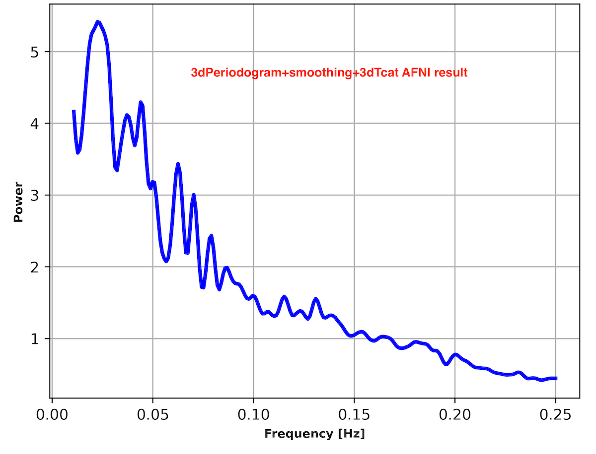
1. I extracted the frequency-domain results from AFNI (the results that were 3dTcat and 3dTsmoothed). These were plotted with Python, shown below. All computations stem from AFNI, Python only plots those.
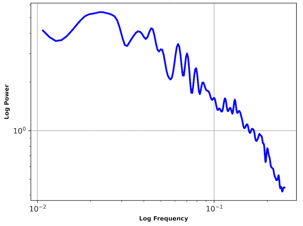
2. I extracted the log-log transformation results from AFNI for the same subject and ROI. These were again plotted with Python.
We can see that a PLE result of -0.01 does really not match the visual results of the log-log transformation; the slope of the curve is far higher (as can already be seen in the frequency-domain without log-log as well). I wonder what is happening here? Does the problem stem from 3dfim+?
Thanks,
Philipp


