9.7. Notes on 3dREMLfit¶

Notes by RW Cox.

9.7.1. Background: time series censoring approaches ¶

A question came up:

Is the way AFNI’s time series regression programs, 3dREMLfit and 3dDeconvolve, deal with time point censoring equivalent to the way that other programs (e.g., SPM, FSL) deal with such censoring?

To understand the alternatives, consider the regression model for a single time series data vector $\mathbf{z}$ with N time points and M regressor (model) component:

$\mathbf{z} = \mathbf{X} \beta + \epsilon$

where $\mathbf{X}$ is an $N\times M$ matrix, $\beta$ is an M-vector, and $\beta$ is the N-vector of residuals (to be made as “small” as possible when solving for $\beta$ ). Suppose that element $\mathbf{z}_i$ is to be censored out of the analysis for whatever silly reason (e.g., too much head motion).

Row removal (AFNI approach): Remove the ith element from $\mathbf{z}$ and correspondingly remove the ith row from the matrix $\mathbf{X}$ (since it is that row which contains the model for $\mathbf{z}_i$ ).
Column augmentation (SPM and FSL approach): Add a column to $\mathbf{X}$ that is all zero except for a single 1 in the ith element. The idea is that this extra regression component will exactly fit the data point in $\mathbf{z}_i$ and so the $\beta$ value for this extra component will be $\mathbf{z}_i$ , and all the other components of beta will be devoted to fitting the “real” data in the rest of vector $\mathbf{z}$ . One column is added for each index i which is to be censored.

The advantages of the row removal method are (a) that it shrinks the $\mathbf{X}$ matrix, reducing the computational load, and (b) that it exactly accounts for the non-use of $\mathbf{z}_i$ since the offending value is omitted entirely from the analysis. The disadvantage of the row removal method is that it breaks the regular time spacing of the data. The column augmentation method has the inverse characteristics.

9.7.2. Are the censoring approaches the same for 3dREMLfit?¶

If some non-AFNI pipeline wants to use 3dREMLfit, the developers are likely to want to censor using the column augmentation method, since that is what most neuroscience people are familiar with. The question arose in my mind about whether the two approaches give the same results in 3dREMLfit.

Regular time spacing is not important if ordinary least squares (OLSQ) is used to fit $\beta$ . However, if a temporal correlation matrix $\mathbf{R}$ needs to be estimated from the data, and then applied to “pre-whiten” the problem, then the temporal spacing needs to be properly allowed for when model-fitting $\mathbf{R}$ and $\beta$ together. Some algorithms for fitting models for R are much simpler with regular (unbroken $\Delta t=TR$ ) time spacing; for example, the Yule-Walker equations for AR(p) models, or even more obviously, DFT-based approaches. AFNI’s 3dREMLfit was built to avoid the requirement for a regular TR, by using a voxelwise ARMA(1,1) model - see 3dREMLfit_mathnotes (RWC’s math notes on 3dREMLfit) for the details. Non-contiguous segments of data (“runs”) can be catenated and analyzed together, as well as allowing for censoring time points where bad things happened. The voxelwise computation of the ARMA(1,1) autocorrelation prewhitening model is meant to allow for different types of temporal correlation structure in different image regions and tissue types. (Is this useful? Opinions vary.)

Aside – Solution methods:

The OLSQ solution is $\beta = [\mathbf{X}^T\mathbf{X}]^{-1} \mathbf{X}^T \mathbf{z}$ . The generalized least squares (GLSQ, or “pre-whitening” solution) is derived by pre-multiplying the matrix-vector equation by a symmetric matrix $\mathbf{W}$ such that $\mathbf{W}^2=\mathbf{R}^{-1}$ , where $\mathbf{R}$ is the temporal autocorrelation matrix. Then the equation becomes $\mathbf{Wz}=\mathbf{WX}\beta +\mathbf{W}\epsilon$ , and under the assumption that $E[\epsilon \epsilon^T] = \sigma^2 \mathbf{R}$ , $E[\mathbf{W}\epsilon \epsilon^T\mathbf{W}] = \sigma^2\mathbf{I}$ , and so this equation is validly/optimally (BLUE) solved by OLSQ, giving instead $\beta = [\mathbf{X}^T\mathbf{R}^{-1}\mathbf{X}]^{-1}\, \mathbf{X}^T\mathbf{R}^{-1} \mathbf{z}$ . The actual calculations in 3dREMLfit are a little more intricate for the sake of efficiency and require estimating $\mathbf{R}$ (using $\epsilon$ ) and $\beta$ together to be self consistent – that’s the point of REML. See the aforementioned math notes for more such “fun”.

Trying it out:

The simplest way to deal with the initial question was to run the program both ways. To aid in doing this, I modified 3dDeconvolve to allow the user (me) to generate the matrix file for 3dREMLfit with censoring handled by column augmentation, in addition to the matrix created with row removal. (3dDeconvolve creates the matrix file for 3dREMLfit, from the user’s time series model components.) 3dREMLfit could then be run twice, once with each censoring method. I used a study which had already been run with afni_proc.py, and started from that results directory.

Script 1: create the two *.xmat.1D files ( $\mathbf{X}$ matrices) in 3dDeconvolve This command was edited from the script generated by afni_proc.py:

3dDeconvolve                                                            \
  -input pb01.sub-10697.r01.tshift+orig.HEAD                            \
  -censor censor_sub-10697_combined_2.1D                                \
  -polort 4 -num_stimts 8                                               \
  -stim_times 1 stimuli/pamenc.times.CONTROL.txt 'BLOCK(2)'             \
    -stim_label 1 CONTROL                                               \
  -stim_times 2 stimuli/pamenc.times.TASK.txt 'BLOCK(4)'                \
    -stim_label 2 TASK                                                  \
  -stim_file 3 'motion_demean.1D[0]' -stim_base 3 -stim_label 3 roll    \
  -stim_file 4 'motion_demean.1D[1]' -stim_base 4 -stim_label 4 pitch   \
  -stim_file 5 'motion_demean.1D[2]' -stim_base 5 -stim_label 5 yaw     \
  -stim_file 6 'motion_demean.1D[3]' -stim_base 6 -stim_label 6 dS      \
  -stim_file 7 'motion_demean.1D[4]' -stim_base 7 -stim_label 7 dL      \
  -stim_file 8 'motion_demean.1D[5]' -stim_base 8 -stim_label 8 dP      \
  -x1D XQ.xmat.1D                                                       \
  -x1D_regcensored XQ.regcensor.xmat.1D                                 \
  -x1D_stop

The -x1D .. and -x1D_regcensored .. options lead to outputting the two *.xmat.1D files for input to 3dREMLfit (row-censored and column-augmented).

Script 2: run 3dREMLfit twice, using the two matrix files, on the time-shifted input data:

3dREMLfit                                                              \
  -matrix XQ.xmat.1D                                                   \
  -input pb01.sub-10697.r01.tshift+orig.HEAD                           \
  -fout -tout -verb -Grid 5                                            \
  -Rbuck QQstats.sub-10697_REML                                        \
  -Rvar QQstats.sub-10697_REMLvar

3dREMLfit                                                              \
  -matrix XQ.regcensor.xmat.1D                                         \
  -input pb01.sub-10697.r01.tshift+orig.HEAD                           \
  -fout -tout -verb -Grid 5                                            \
  -Rbuck QQRstats.sub-10697_REML                                       \
  -Rvar QQRstats.sub-10697_REMLvar

... and then the stats datasets from the two runs can be compared (visually and by subtraction).

It turned out that the results were exactly the same, except in a few voxels – about 10 out of more than 300,000. This outcome was peculiar, but a few moments of inspection showed that the differences occurred precisely in those (non-brain) voxels which were identically 0 except at one or more of the censored time points. When I realized this, the explanation was obvious.

With row removal, the censored data points are fully removed from the analysis. In these exceptional voxels, that removal resulted in the data time series $\mathbf{z}$ being identically zero. When this happens, 3dREMLfit skips all analysis in that voxel, and fills in the corresponding voxel results as being all zeros. In column augmentation, normal linear solving will take place, as the data is not exactly zero. In exact arithmetic solution, the augmented columns would zero out the nonzero elements of $\mathbf{z}$ ; however, with inexact computer arithmetic, the linear regression leaves a nonzero residual vector $\epsilon$ , which in turn is analyzed for the ARMA(1,1) parameters, and then $\beta$ and all the voxel-level statistics are calculated. Question answered: 3dREMLfit works the same for either censoring method.

But ... there’s always a “but”:

In looking at the results from Script 2, I saw something peculiar:

Structure in the $\lambda$ parameter (sagittal image)

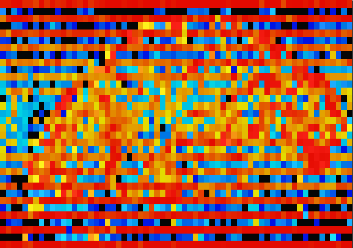
Output from `3dREMLfit`

This is an image of the $\lambda$ parameter = correlation at lag=1 from the ARMA(1,1) model. A little thought shows that this is due to the time-shifting operation. By default, the necessary temporal interpolation is done with 5th order (quintic) Lagrange polynomials, which uses $\pm2$ points in time for interpolation (via AFNI program 3dTshift). I re-ran the time shifting with the various options for interpolation method, and found that the Fourier (FFT) interpolation completely eliminated the stripes. To further investigate, I added $\pm5$ and $\pm9$ point weighted sinc interpolation methods to 3dTshift. The striping artifact is reduced with the “wsinc5” method, and almost completely gone with the “wsinc9” method.

How important is this artifact? If one is using 3dREMLfit, then the voxelwise ARMA(1,1) model should deal with it. The alternative cure, using a broader-based temporal interpolation, gets rid of the artifact, but has the downside that more distant time points will leak into the interpolated output values. In turn, this could bias the $\beta$ estimation – probably not much, but that is another line for investigation.

Conclusion: The Rabbit Hole Has No Bottom.

9.7.3. Attributes in the 3dREMLFIT *.xmat.1D format ¶

Attributes are stored in an XML-ish header before the actual matrix numbers. Attributes are of the form name = "quoted string" - the quotes can be single or double.

Below is a sample header, followed by the first row of the matrix (there are 444 rows in the actual matrix, each with 20 numbers):

# <matrix
#  ni_type = "20*double"
#  ni_dimen = "444"
#  ColumnLabels = "Run#1Pol#0 ; Run#1Pol#1 ; Run#1Pol#2 ; Run#1Pol#3 ; Run#2Pol#0 ; Run#2Pol#1 ; Run#2Pol#2 ; Run#2Pol#3 ; Run#3Pol#0 ; Run#3Pol#1 ; Run#3Pol#2 ; Run#3Pol#3 ; vis#0 ; aud#0 ; roll#0 ; pitch#0 ; yaw#0 ; dS#0 ; dL#0 ; dP#0"
#  ColumnGroups = "12@-1,1,2,6@0"
#  RowTR = "2"
#  GoodList = "0..40,45..264,267..449"
#  NRowFull = "450"
#  RunStart = "0,150,300"
#  Nstim = "2"
#  StimBots = "12,13"
#  StimTops = "12,13"
#  StimLabels = "vis ; aud"
#  Nglt = "1"
#  GltLabels = "V-A"
#  GltMatrix_000000 = "1,20,12@0,1,-1,6@0"
#  BasisNstim = "8"
#  BasisOption_000001 = "-stim_times"
#  BasisName_000001 = "vis"
#  BasisFormula_000001 = "BLOCK(20,1)"
#  BasisColumns_000001 = "12:12"
#  BasisOption_000002 = "-stim_times"
#  BasisName_000002 = "aud"
#  BasisFormula_000002 = "BLOCK(20,1)"
#  BasisColumns_000002 = "13:13"
#  CommandLine = "3dDeconvolve -input pb05.FT.surf.rh.r01.scale.niml.dset pb05.FT.surf.rh.r02.scale.niml.dset pb05.FT.surf.rh.r03.scale.niml.dset -censor motion_FT.surf_censor.1D -polort 3 -num_stimts 8 -stim_times 1 stimuli/AV1_vis.txt &apos;BLOCK(20,1)&apos; -stim_label 1 vis -stim_times 2 stimuli/AV2_aud.txt &apos;BLOCK(20,1)&apos; -stim_label 2 aud -stim_file 3 &apos;motion_demean.1D[0]&apos; -stim_base 3 -stim_label 3 roll -stim_file 4 &apos;motion_demean.1D[1]&apos; -stim_base 4 -stim_label 4 pitch -stim_file 5 &apos;motion_demean.1D[2]&apos; -stim_base 5 -stim_label 5 yaw -stim_file 6 &apos;motion_demean.1D[3]&apos; -stim_base 6 -stim_label 6 dS -stim_file 7 &apos;motion_demean.1D[4]&apos; -stim_base 7 -stim_label 7 dL -stim_file 8 &apos;motion_demean.1D[5]&apos; -stim_base 8 -stim_label 8 dP -jobs 2 -gltsym &apos;SYM: vis -aud&apos; -glt_label 1 V-A -fout -tout -x1D X.xmat.1D -xjpeg X.jpg -x1D_uncensored X.nocensor.xmat.1D -fitts fitts.FT.surf.rh.niml.dset -errts errts.FT.surf.rh.niml.dset -bucket stats.FT.surf.rh.niml.dset"
# >
1 -0.99999999284744 0.9932885915041 -1.0000000007947 0 0 0 0 0 0 0 0 0 0 -0.056317329311536 0.1472171255615 -0.030924689328919 -0.14155002441671 -0.0522833100934 -0.081843944456843

For computational details, idly peruse this scan of my handwritten notes about 3dREMLfit’s algorithms and models:

RWC’s math notes on 3dREMLfit

Some attributes are necessary for 3dREMLfit to operate, and some are optional. The leading '#' character on each line is not necessary, and is there for peculiar historical/hysterical reasons and also for compatibility with some other AFNI software (e.g., 1dplot).

Attributes can be in any order inside the <matrix ... > header.

Note that index counting (e.g., for rows and columns, mentioned below) starts at 0, not 1, as decreed by the Almighty.

ni_type = "20*double"
- [REQUIRED]
- This indicates there are 20 numerical values per row in the data section (past the header), and they are to be interpreted as doubles (64 bit floating point values) when read in.
- In this example, the matrix has 20 columns (regressors) – numbered from 0..19, as mentioned above.
- In the code, this numeric value (20) is called nreg = number of regressors; that is how I will refer to it below, as needed.
- The "*double" is needed, since the parser for this format allows data columns of various types, but in this case all the data columns are numeric.
ni_dimen = "444"
- [REQUIRED]
- This value indicates there are 444 rows in the data section.
- In this example, the matrix corresponds to 444 time points (TRs).
- Also see NRowFull below.
ColumnLabels = "Run#1Pol#0 ; Run#1Pol#1 ; Run#1Pol#2 ; Run#1Pol#3 ; Run#2Pol#0 ; Run#2Pol#1 ; Run#2Pol#2 ; Run#2Pol#3 ; Run#3Pol#0 ; Run#3Pol#1 ; Run#3Pol#2 ; Run#3Pol#3 ; vis#0 ; aud#0 ; roll#0 ; pitch#0 ; yaw#0 ; dS#0 ; dL#0 ; dP#0"
- [OPTIONAL but highly recommended]
- Defines the string label for each column in the matrix.
- If this attribute is present, there must be as many labels as columns (nreg).
- Labels cannot contain whitespace characters unless ‘in quotes’.
  - In this example, single quotes would have to be used, to distinguish from the double quotes used to delineate the attribute itself.
- Labels must be separated as shown above, with a semicolon (labels can contain commas, if you insist).
- In this example, columns 0..11 and 14..19 are regressors of no interest, and columns 12 and 13 (vis#0 and aud#0) are the regressors of interest (response models for stimuli).
  - Which regressors correspond to stimuli and which do not will be marked out in the 'Stim' attributes described later.
- Labels are attached to output volumes in the results datasets, to make it easy for the AFNI user to see which volume corresponds to the statistical estimates for which stimulus.
ColumnGroups = "12@-1,1,2,6@0"
- [NOT USED]
- This attribute is not actually used by 3dREMLfit for anything at this time [Aug 2019].
- Its intended function is to mark matrix columns as being in different groups. In this example, the first 12 columns are “baseline and drift model” (group -1), the next 2 columns belong to distinct stimuli, and the last 6 columns belong to the motion regressors (and other dataset-based) regressors of no interest.
RowTR = "2"
- [OPTIONAL]
- This attribute is not actually used by 3dREMLfit now [Aug 2019].
- It defines the inter-scan time interval (TR) in seconds. The TR is needed for construction of the matrix from the stimulus response model, but that has already been done, so this attribute is really just for documentation and completeness.
GoodList = "0..40,45..264,267..449"
- [HIGHLY REQUIRED]
- The matrix provided to 3dREMLfit is the censored matrix; that is, the time points (TRs) to be censored have had the corresponding rows removed from the full matrix.
  - The data volumes to be censored will be removed from the input dataset during processing by 3dREMLfit.
- The GoodList attribute lists the TR indexes from the original (uncensored) time series dataset that are present in the matrix file; that is, it is the opposite of the “censor list”.
- There must be the same number of integers specified here as the number of time points specified by the ni_dimen attribute (here, 444).
- The brute force approach would be just to list all the integers, comma separated, in one long string.
- For the sake of compactness, contiguous sequences of integers can be given, as in the example, where "0..40" means the same as listing all the integers 0, 1, 2, ..., 40.
- In this example, there were 450 time points in the original EPI dataset, and clearly 6 of them have been censored, since the matrix has only 444 rows.
  - This attribute is required so that the temporal autocorrelation ARMA(1,1) voxelwise model doesn’t falsely assume that the data to be processed occurs with constant TR.
  - The RunStart attribute (below) subserves this purpose also, marking the temporal discontinuities between multiple EPI imaging runs.
  - If there were no censoring, then GoodList = "0..449" would work fine (but still would be required by 3dREMLfit).
NRowFull = "450"
- [REQUIRED]
- This attribute gives the number of TRs in the full (uncensored matrix).
- It is needed for creating the “fitts” and “errts” output datasets, and also for consistency checking to make sure that the user is inputting data that matches the matrix.
RunStart = "0,150,300"
- [OPTIONAL]
- If there is more than one imaging run – that is, there is a long temporal discontinuity between some time points in the dataset to be processed – then this attribute gives the list of the starting TR indexes for each run.
- In this example, there were 3 runs of 150 TRs each: 0..149, 150..299, and 300..499.
  - The ARMA(1,1) model for the noise temporal correlation is built to have zero correlations for time point pairs from different runs; see the math notes for details on how this is implemented.
- As with GoodList, this attribute is needed for correct temporal autocorrelation model fitting.
- If RunStart is not present, then the input EPI dataset is presumed to contain only one imaging run.
The "Stim" group of attributes mark off some columns as being “of interest” for statistics – presumably from task stimuli. These are [OPTIONAL] as a group, but if Nstim is present, then the others must be present as well.
- Statistics (betas and t-statistics) will be computed only for columns marked as belonging to stimuli, since no one is ever interested in the statistics for the drift and motion parameters (e.g.). If the "Stim" attributes are not present, statistics will not be calculated unless GLTs are used.
- Nstim = "2"
  - This attribute indicates how many distinct stimuli present.
  - Each stimulus will correspond to 1 or more contiguous columns in the matrix.
- StimBots = "12,13"
  - This attribute should have Nstim integer entries.
  - It indicates the column indexes (remember, counting starts at 0) that correspond to the start of each stimulus’s column group.
- StimTops = "12,13"
  - This attribute should have Nstim integer entries.
  - It indicates the column indexes that correspond to the end of each stimulus’s column group.
  - In this example, the model for each stimulus has just one column, so the StimBots and StimTops attributes are identical.
  - In deconvolution type models (e.g., AFNI TENTS, FIR models) or in parametric regression, a single stimulus will have multiple regression columns in its response model.
- StimLabels = "vis ; aud"
  - This attribute should have Nstim string entries, separated by semicolons.
  - These are used (among other things) to process symbolic general linear tests (GLTs) among beta coefficients, given on the 3dREMLfit command line via the "-gltsym" option.
The “GLT” group is used to specify one or more general linear tests among the beta coefficients, directly in the matrix file. These are completely [OPTIONAL].
- As mentioned above, GLTs can also be specified outside the matrix file, on the 3dREMLfit command line.
  - GLTs in the matrix file are specified as sets of coefficients to be applied to the beta estimates.
  - GLTs on the 3dREMLfit command line can use symbolic names for the stimuli to specify the coefficients to be attached to the betas.
- Nglt = "1"
  - If present, this attribute specifies the number of GLTs in the matrix file. It should be an integer from 1 to 1000000.
  - GltLabels = "V-A"
    - This attribute contains Nglt string labels, one for each GLT specified.
    - The labels are attached to the output data volumes to make it easy for the user to see which volume corresponds to what statistical test.
  - GltMatrix_000000 = "1,20,12@0,1,-1,6@0"
    - There should be Nglt of these attributes, with a six digit suffix starting at _000000, then _000001, and so forth. (If you want more than 1 million GLTs, you are legally insane and should be confined for your own safety.)
    - Each GltMatrix_xxxxxx attribute has r＊nreg+2 numeric values, which are used to define an $r \times nreg`$ matrix for some $r \geq 1`$ .
      - The first value in the attribute is the number of rows r in the GLT matrix.
      - r = 1 corresponds to a t-test of the weighted sum of betas against the null hypothesis that the sum is 0.
      - r > 1 corresponds to an F-test of the r weighted beta sums defined by the individual rows against the null hypothesis that these sums are all zero.
    - The second value in the attribute is the number of columns in the GLT matrix.
      - This value must be the same as nreg, or 3dREMLfit will not like the matrix file (i.e., it will exit with an error message). It is present here to make the matrix definition self-contained, and as a check that the creator of the matrix file is not deranged.
    - The remaining values are the rows of the GLT matrix, nreg numbers per row, r rows, row after row.
      - In the example, there are only 2 nonzero numbers in the single row, corresponding (naturally) to the test vis-aud≟0.
      - There is no requirement that a GLT be a “contrast”; that is, the sum of the weights in the rows do not need to be 0.
The “Basis” group of attributes is [NOT USED] by 3dREMLfit at this time.
- I won't describe them now, since this exercise is really getting dull.
  - Their function is to describe the response model used to construct the stimulus columns, and the example above is from AFNI program 3dDeconvolve.
- I don’t even recall why I put this stuff in here (for Rick Reynolds, maybe?).
CommandLine = "3dDeconvolve -input ......"
- [OPTIONAL]
  
  This option is used to write the command that generated the matrix file into the output dataset(s) history note, for the potential elucidation of any user of the data. Otherwise, it is not needed or used.

9.7. Notes on 3dREMLfit¶

9.7.1. Background: time series censoring approaches ¶

9.7.2. Are the censoring approaches the same for 3dREMLfit?¶

9.7.3. Attributes in the 3dREMLFIT *.xmat.1D format ¶

Table of Contents

This Page

Quick search

9.7. Notes on 3dREMLfit¶

9.7.1. Background: time series censoring approaches¶

9.7.2. Are the censoring approaches the same for 3dREMLfit?¶

9.7.3. Attributes in the 3dREMLFIT *.xmat.1D format¶

9.7.1. Background: time series censoring approaches ¶

9.7.3. Attributes in the 3dREMLFIT *.xmat.1D format ¶