SUMA Controller To control aspects common to all
the SUMA viewers.
Viewer Controller: To control aspects particular to one viewer. This
baby is practically nonexistent at this stage.
Object Controllers: To control how certain objects and the data
defined over them are displayed. In modern SUMA versions, it is best
that all controllers are collected in the same controller
notebook. Example controllers include the
Surface Controller, the Tract
Controller, the Volume Controller etc.
The suma controller is for controlling parameters common to across viewers and objects.You can launch the Suma Controller with: ctrl+u or View‣Suma Controller
Close SUMA controller window.
Current settings are preserved
when controller is reopened.
done: Click twice in 5 seconds to close everything and quit SUMA.
Click twice in 5 seconds to quit application. All viewer windows will be closed, nothing is saved, SUMA will terminate, and there maybe no one left at this computer.
Many of the displayable objects, particularly those that can
carry data, have an object controller. Historically there was
only surface-controllers (hence the Ctrl+s for the shortcut)
but now volumes, tracts, and graphs also have their own
controllers.
The easiest way to open a controller is to select an object and
open its controller with ctrl+s, or View
‣ Object Controller. Once a controller is open, selecting
other objects automatically creates their own controller.
All object controllers are grouped in one notebook window as
shown in Object Controller. If you don’t have all your object
controllers opening in the same notebook and your SUMA version
is current, make sure environment variable
SUMA_SameSurfCont is set to YES in
your .sumarc file.
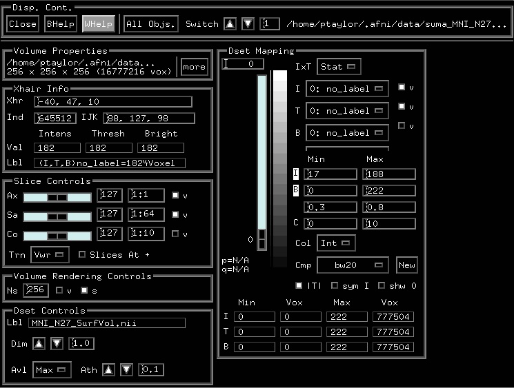
Object Controller Notebook: Holder of all controllers. Grayed
out area will be different for different object
types. (link)
Once you select an object, its controller is popped to the
top. You can also use the Switch to get at
the controller for an object that you don’t want to select or
that is simply out of reach (invisible).
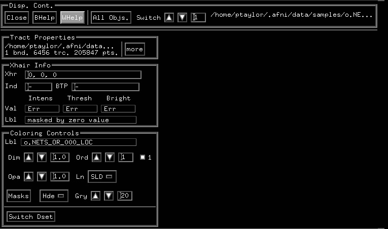
Disp. Cont.
A few controls for the object controller notebook.
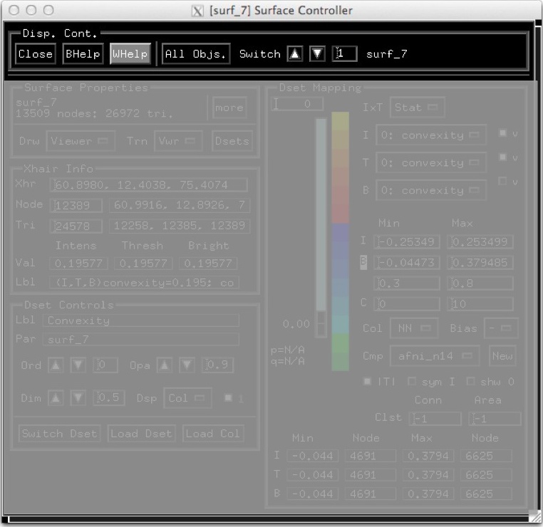
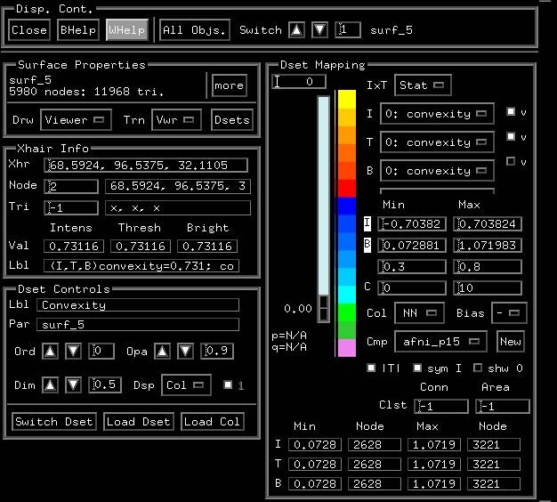
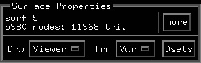
The surface controller is for controlling the way surfaces and datasets defined over them are displayed. The same controller is shared by a family of surfaces and all the datasets displayed on them. Left and Right surfaces have separate controllers though in most cases actions on one hemisphere’s controller are automatically mirrored on the contralateral side. The surface controller is initialized by the currently selected surface - the one said to be in focus.
You can launch the Surface Controller with: ctrl+s or View‣Object Controller
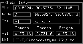
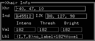
Set/Get crosshair location in mm RAI on
this controller’s selected object.
Entering new coordinates
makes the crosshair jump
to that location (like ‘ctrl+j’).
Use ‘alt+l’ to center the
cross hair in your viewer.
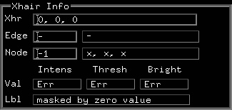
Index of node in focus (1) and RAI coordinates of that node (2).
1- The index is of the node in focus on this controller’s surface. Nodes in focus are highlighted by the blue sphere in the crosshair.
This cell is editable; manually entering a new node’s index will put that node in focus and send the crosshair to its location (like ‘j’). Use ‘alt+l’ to center the cross hair in your viewer.
2- The RAI coordinates are those of the surface node after all spatial transformations have been applied to the surface. Those transformations do not include visualization transformations applied in the viewer
1- Triangle (faceset) index of triangle in focus on this on this controller’s surface.
Triangle in focus is highlighted in gray, and entering a new triangle’s index will set a new triangle in focus (like ‘J’).
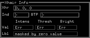
Data values at node in focus. Intensity, Threshold, and Brightness show the triplets of values at the selected node that correspond to the dataset column choices in I, T, and B selectors.
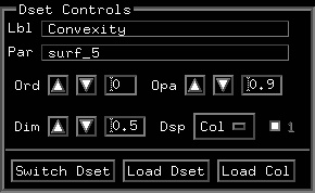
Label of dataset currently selected. Note that for some objects, like surfaces, what you’re viewing at any moment maybe a blend of multiple datasets. See color mixing for details.
Order of Dset’s colorplane in the stack of all colorplanes of the parent surface.
The datset with highest order number is
on top of the stack. Separate
stacks exist for foreground (fg:)
and background planes (bg:).
See Color Mixing for details on how colors are merged.
Opacity of Dset’s colorplane.
Opaque planes have an opacity
of 1, transparent planes have
an opacity of 0.
Opacities are used when mixing
planes within the same group
foreground (fg:) or background(bg:).
Opacity values are not applied
to the first plane in a group.
Consequently, if you have just
one plane to work with, opacity
value is meaningless.
Color mixing can be done in two
ways, use F7 to toggle between
mixing modes.
Dim: Dimming factor to apply to colormap or color datasets.
Dimming factor to apply to colormap
before mapping the intensity (I) data.
The colormap, if displayed on the right,
is not visibly affected by Dim but the
colors mapped onto the surface, voxel grid, tracts, etc. are.
For RGB Dsets (e.g. .col files, or tract colors), Dim is
applied to the RGB colors directly.
Decreasing Dim is useful when the colors are too saturated
for lighting to reflect the object terrain.
When in doubt, just press the button and see what happens.
There is one contour created for each color in the colormap. You’d want to use colormaps with few colors to get a contour of use. Contours are not created if colormap has panes of unequal sizes.
Each row i contains Nj data values per node.Since this format has no headerassociated with it, it makessome assumption about the datain the columns.
You can choose from 3 options: (see below for nomenclature)
Each column has Ni values where Ni = N_Node. In this case, it is assumed that row i has values for node i on the surface.
If Ni is not equal to N_Node then SUMA will check to see if column 0 (Col_0) is all integers with values v satisfying: 0 <= v < N_Node .
If that is the case then column 0 contains the node indices. The values in row j of Dset are for the node indexed Col_0[j].
In the sample 1D Dset shown below assuming N_Node > 58, SUMA will consider the 1st column to contain node indices. In that case the values -12.1 and 0.9 are for node 58 on the surface.
Lastly, if Col_0 fails the node index test, then SUMA considers the data in row i to be associated with node i.
If you’re confused, try creating some toy datasets like the one below and load them into SUMA.
Sample 1D Dset (Call it pickle.1D.dset):
25 22.7 1.2
58 -12.1 0.9
Nomenclature and conventions:
N_Node is the number of nodes forming the surface.
Indexing always starts at 0. In the example, value v at row 0, column 1 is v = 22.7 .
A Dset has Ni rows and Nj columns. In other terms, Ni is the number of values per node and Nj is the number of nodes for which data are specified in Dset. Ni = 2, Nj = 3 in the example.
Load a new color plane.
A color plane is a 1D text file with
each row formatted as such
n r g b
where n is the node index,
r, g, and b are the red, green and blue
color values, respectively.
Color values must be between 0 and 1.0.
A sample file would be: test.1D.col with content:
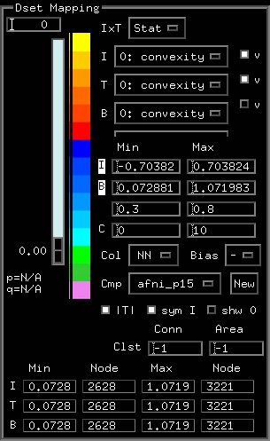
Use this menu to select which column (sub-brick) in the dataset (Dset) should be used for an Intensity (I)measure.
Values in (I) are the ones that get colored by the colormap,however, no coloring is done if the ‘v’ button on the right isturned off.
The (I) value for the selected datum (n) is shown in the ‘Val’ tableof the ‘Xhair Info’ section on the left.
The value is also shown in the SUMA viewer
You can use a different type of selector to set (I). A right-click on ‘I’ opens a list widget, which is better when you have many columns from which to choose.
The style of this selector can also change depending on the numberof sub-bricks (columns) you have in your dataset. If the numberexceeds a threshold specified by the environment variable SUMA_ArrowFieldSelectorTrigger
Thresholding is not applied when the ‘v’ button on the right is turned off.
The (T) value for the selected datum (n) is shown in the ‘Val’ tableof the ‘Xhair Info’ section on the left.
The value is also shown in the SUMA viewer
You can use a different type of selector to set (T). A right-click on ‘T’ opens a list widget, which is better when you have many columns from which to choose.
The style of this selector can also change depending on the number of sub-bricks (columns) you have in your dataset. If the number exceeds a threshold specified by the environment variable SUMA_ArrowFieldSelectorTrigger
Use this menu to select which column (sub-brick) in the dataset (Dset) should be used for color Brightness (B) modulation.
The (B) values are the ones used to control the brightness of a datum’s color.
Brightness modulation is controlled by ranges in the ‘B’ cells of the table below.
Brightness modulation is not applied when the ‘v’ button on
the right is turned off.
The (B) value for the selected datum (n) is shown in the ‘Val’ tableof the ‘Xhair Info’ section on the left.
The value is also shown in the SUMA viewer
You can use a different type of selector to set (B). A right-click on ‘B’ opens a list widget, which is better when you have many columns from which to choose.
The style of this selector can also change depending on the numberof sub-bricks (columns) you have in your dataset. If the numberexceeds a threshold specified by the environment variable SUMA_ArrowFieldSelectorTrigger
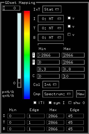
Colorbar used for colorizing values in ‘I’ sub-brick.
Colorization depends on the settings under the I, Range Setting, among other things. Threshold settings determine whether or not a certain value will get displayed at all.
Set threshold value to determine which nodes/voxels/edges will get coloredVoxels for which the value in the ‘T’ sub-brick is below that of the threshold will not get colored.
Used for setting the clipping ranges. Clipping is only done for
color mapping. Actual data
values do not change.
SetRangeTable.r01: Intensity clipping range (append ‘%’ for percentiles, see BHelp)
Intensity clipping range rules:
Values in the intensity data that are less than Min are colored by the first (bottom) color of the colormap.
Values larger than Max are mapped to the top color.
Intermediate values are mapped according to the ‘Col’ menu below.
You can set the range as a percentile of the dataset’s values by appending ‘%’ to the percentile for Min and/or Max such as 5% or 90%. Note that the percentile always gets replaced by the actual value in the dataset.
A left-click on ‘I’ locks ranges from automatic resetting, and the locked range applies to the current Dset only. A locked range is indicated with the reverse video mode.
A right-click resets values to the default range (usually 2% to 98%) in the dataset.
Values in the brightness (B) column are clipped to the Min to Max range in this row before calculating their modulation factor per the values in the next table row.
You can set the range as a percentile of the dataset’s values by appending ‘%’ to the percentile for Min and/or Max such as 8% or 75%. Note that the percentile always gets replaced by the actual value in the dataset.
A left-click locks ranges in this row from automatic resetting, and a locked range is applied to the current Dset only. A locked range is indicated with the reverse video mode.
A right-click resets values to the default range (usually 2% to 98%) for the dataset.
Brightness modulation factor range.
Brightness modulation values, after
clipping per the values in the row above,
are scaled to fit the range specified
here.
Switch between modes for mapping values to the color map.
The bottom color of the map C0 maps to the minimum value in the I range row, and the top color to the maximum value. Colors for values in between the minimum and maximum of I range, the following methods apply
Int: Interpolate linearly between colors in colormap to find color at
icol=((V-Vmin)/Vrange * Ncol)
NN : Use the nearest color in the colormap. The index into the colormap of Ncol colors is given by
icol=floor((V-Vmin)/Vrange * Ncol)
with icol clipped to the range 0 to Ncol-1
Dir: Use intensity values as indices into the colormap. In Dir mode, the intensity clipping range is of no use.
icol=floor(V) with clipping to the range 0 to Ncol-1
Switch between available color maps.
If the number of colormaps is too large
for the menu button, right click over
the ‘Cmp’ label and a chooser with a
slider bar will appear.
More help is available via
ctrl+h while mouse is over the
colormap.
Minimum distance between nodes.
Nodes closer than the minimum distance are in
same cluster. If you want to distance to be in
number of edges (N) separating nodes, set the minimum
distance to -N. This parameter is the same as -rmm in
the program SurfClust
Node index at minimum.
Right click in cell to
have crosshair jump to
node’s index.
Same as ‘ctrl+j’ or
an entry in the ‘Node’ cell
under Xhair Info block.
Node index at maximum.
Right click in cell to
have crosshair jump to
node’s index.
Same as ‘ctrl+j’ or
an entry in the ‘Node’ cell
under Xhair Info block.
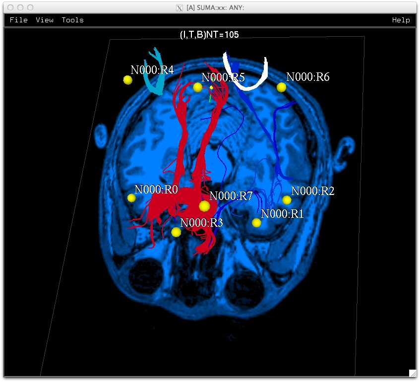
The tract controller is for controlling the way tracts and values defined over them are displayed. Each network of tracts gets its own controller. You can launch the Tract Controller with: ctrl+s or View‣Object Controller
Set/Get crosshair location in mm RAI on
this controller’s selected object.
Entering new coordinates
makes the crosshair jump
to that location (like ‘ctrl+j’).
Use ‘alt+l’ to center the
cross hair in your viewer.
Data values at point in focus. At the moment, Intensity, Threshold, and Brightness show the RGB values for the point selected. Eventually, they would represent the triplets of values at the point that correspond to the dataset column choices in I, T, B.
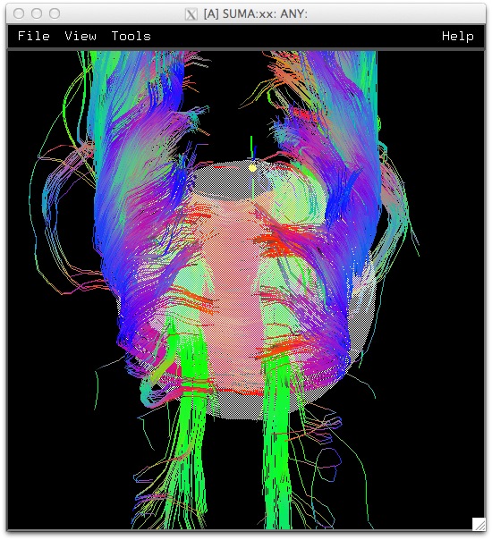
Controls the final coloration of the tracts based on the tract datasets available. What’s a tract dataset you say? It is a dataset defined over the collection of points that define the tracts of a network. And where do we get these sets? Nowhere at the moment. For now they are generated internally and they are only of the RGB variety. This will change in the future, when you would be able to drive a flying car and have arbitrary sets much like on surfaces or volumes.
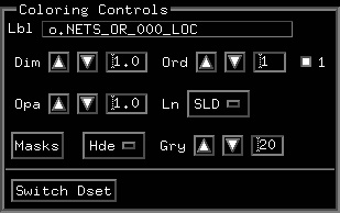
Label of dataset currently selected. Note that for some objects, like surfaces, what you’re viewing at any moment maybe a blend of multiple datasets. See color mixing for details.
Dim: Dimming factor to apply to colormap or color datasets.
Dimming factor to apply to colormap
before mapping the intensity (I) data.
The colormap, if displayed on the right,
is not visibly affected by Dim but the
colors mapped onto the surface, voxel grid, tracts, etc. are.
For RGB Dsets (e.g. .col files, or tract colors), Dim is
applied to the RGB colors directly.
Decreasing Dim is useful when the colors are too saturated
for lighting to reflect the object terrain.
When in doubt, just press the button and see what happens.
Order of this tract’s dataset colorplane in the stack of all colorplanes available.
The datset with highest order number is
on top of the stack.
See color plane grouping for details on how colors are merged.
Opacity of Dset’s colorplane.
Opaque planes have an opacity
of 1, transparent planes have
an opacity of 0.
Opacity values are not applied
to the first plane in a group.
Consequently, if you have just
one plane to work with, or you have 1 ON,
the opacity value is meaningless.
Color mixing can be done in two
ways, use F7 to toggle between
mixing modes.
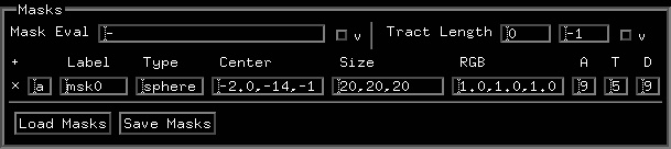
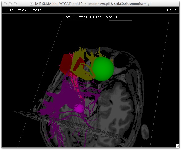
Opens controller for masks.
At the first click, this button creates a new interactive tract mask and activates menu items such as Gry. A ball of a mask is added to the interface, and only tracts that go through it are displayed.
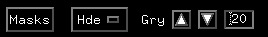
That’s not the name of the button, but its default value. This menu controls how tracts that fall outside of the masks are displayed:
Hde: Hide ‘em masked tracts
Gry: Gray ‘em masked tracts (gray color set by Gry arrow field)
One: A coding mistake that ended up looking cool. Each tract not in the mask is colored by one color extracted from the set of colors for the whole network.
Ign: Ignore ‘em good for nothing masks, show tracts in all their unabashed glory
Gry: Gray level (0–100) of tracts outside of mask (only for Msk –> Gry)
Set the gray level for masked tracts. 0 for black, 100 for white
This arrow field only has an effect when ‘Msk’ menu is set to ‘Gry’
Select the dataset to which the Coloring Controls are being applied. For now you have three free RGB datasets per network that are created by SUMA. In the first one each node of a tract is colored based on the local orientation, with red, green, and blue values reflecting the X,Y, and Z components of the unit direction vector. In the second dataset all nodes of a tract are assigned the color of the middle node of that tract. In the third dataset, all nodes of a tract are colored based on the bundle in which that tract resides.The number of colors in such a dataset depend on the total number of bundles in the entire network.
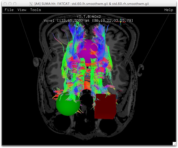
To move the mask interactively, right-double click on it to place SUMA in Mask Manipulation Mode which is indicated by displaying the moveable mask in mesh mode (see help in SUMA, (ctrl+h), section Button 3-DoubleClick for details.). Selecting a location on the tracts, the slices, or surfaces, will make the mask jump to that location. The mask should also be visibile in AFNI (if SUMA is launched with -dev option), and clicking in AFNI will make the mask move in SUMA also.
To turn off ‘Mask Manipulation Mode’ right-double click in open air, or on the manipulated mask itself.
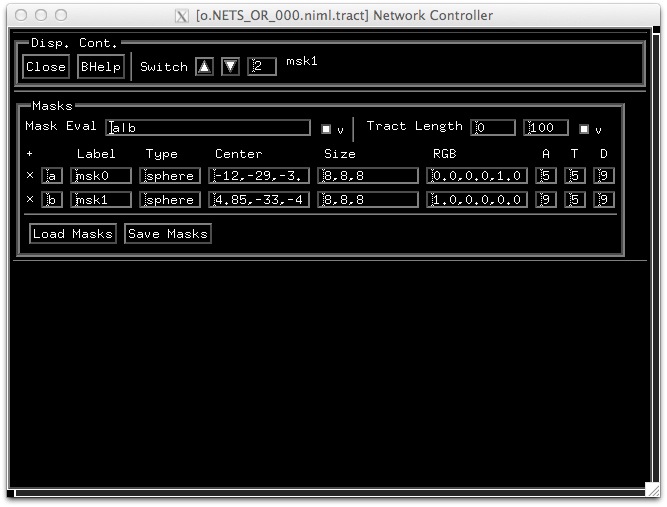
The mask controller is used for manipulating masks for network tractsYou can launch the Mask Controller from the tract controller by clicking on Masks twice.
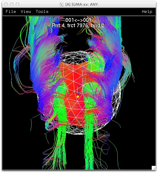
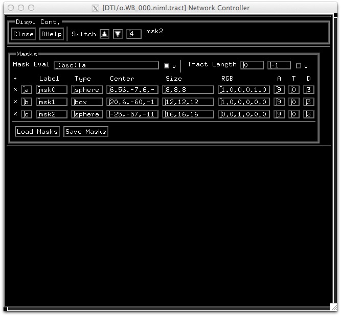
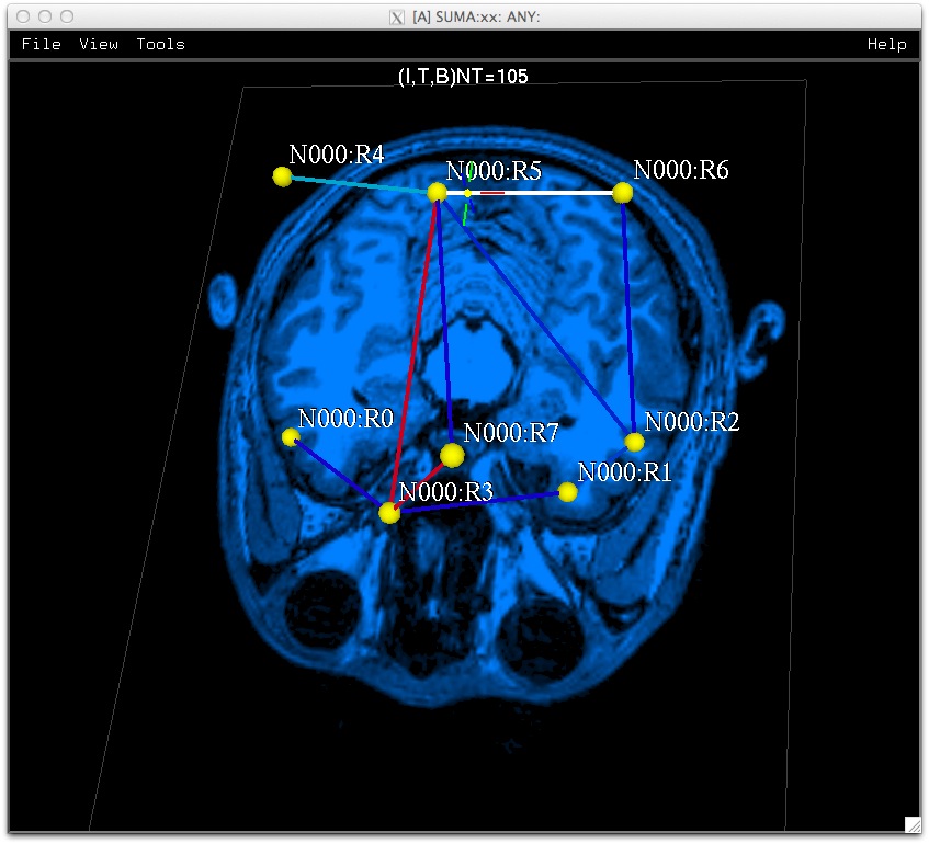
A boolean expression evaluated per tract to determine whether or not a tract should be displayed. Each mask is assigned a letter from ‘a’ to ‘z’ and has an entry in the table below. Symbols for the OR operator are ‘|’ or ‘+’ while those for AND are ‘&’ or ‘*’. The ‘|’ is for the NOT operation. By default, the expression is blank, as indicated by ‘-’, and the operation is an OR of all the masks.
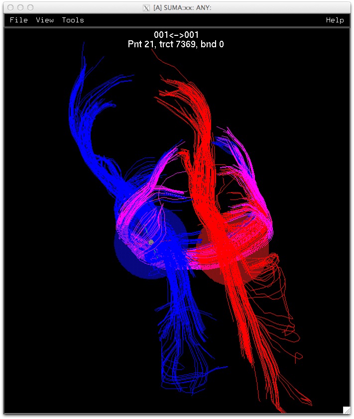
Tracts that go through any of the masks are displayed and they keep their own color, as shown in the figure below to the left.
Say we now want to show tracts that go through both masks b and c or through mask a. The expression to evaluate at each tract would be: ‘( b & c ) | a’. Note that for the expression to take effect, you need to have the v button selected.
When using the the Mask Eval expression, the color of tracts that go though a set of regions is equal to the alpha weighted average of the colors of those regions. This can be seen in the figure on the right side above.
The colors of a tract is given by:
Ct= sum(AiCi)/sum(Ai)
for all ROIs i the tract intersects.
For example, say a tract goes through a blue region of color [0 0 1] with alpha of 0.5 (A ~ 5 in column A), and a red region of color [1 0 0] (alpha is 1.0, or in the table = 9). The tracts that go through both ROIs will be colored (1.0*([1 0 0]+0.5*([0 0 1])/1.5, which is purple. Similar averaging goes on if tracts go through more than 2 regions. Tracts that go though one region will get that region’s color.
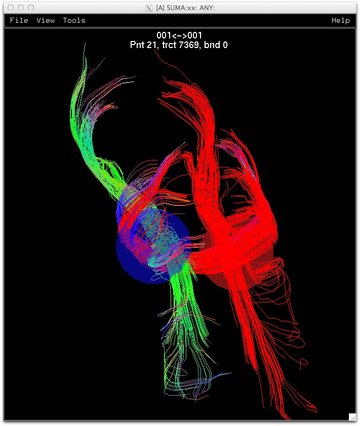
Now, if you set alpha to 0 for a certain ROI, then that ROI does add to the tint of tracts that go thourough it at all. And for a tract that goes through that region only, it retains its original colors. See image on the right side.
Tracts going through any of 2 masks ‘a|b’, with ‘Mask Eval’ ON. (link)
Tracts going through ‘a|b’ but with alpha of ROI ‘a’ - the blue one - set to 0. Tracts going through the blue ROI are not tinted by it at all. (link)
Mask Controller settings for image to the left. (link)
Set Min Max length for tract masking. Use can scroll (mouse wheel) in Min and Max cells to change the value. The ‘v’ button must be selected for masking to take effect.
Alpha of mask color. The Alpha value controls the contribution of an ROI’scolor to the tracts that pass through it. This tinting process is only used when ‘Mask Eval’ is in use, and when A is > 0. See the help for ‘Mask Eval’ for information on how tinting works.
You can also change values by scrolling with mouse pointer over the cell.
Dimming factor for color. Saturated colors may not look nice when rendered, so consider using the D parameter to dim a color’s brightness without having to so directly in the color column. Setting D to 6 for example will scale a color by a factor of 6/9, so a saturated red of [1 0 0] becomes [0.67 0 0 ]. This makes masks render better when not in transparent mode T = 0.
You can also change values by scrolling with mouse pointer over the cell.
The volume controller is for controlling the way volumes are rendered. Each volume gets its own controller. You can use the switch button above to switch between them. The volume controller is initialized by the volume of the last selected voxel.
After you have selected a voxel, you can launch the Volume Controller with: ctrl+s or View‣Object Controller
Set/Get crosshair location in mm RAI on
this controller’s selected object.
Entering new coordinates
makes the crosshair jump
to that location (like ‘ctrl+j’).
Use ‘alt+l’ to center the
cross hair in your viewer.
Data values at voxel in focus. Intensity, Threshold, and Brightness show the triplets of values at the selected voxel that correspond to the volume column choices in I, T, and B selectors.
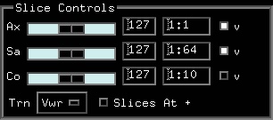
Ax: Select axial slice(s) to render (use BHelp for details)
Select axial slice(s) to render.
If the dataset is oblique, that would be the slice that is closest
to the axial plane.
Move slider bar or enter slice number directly in adjoining field.
To show a stack of axial slices set the second text field to N:S
where N is the number of slices in the stack and S is the spacing
in number of slices between consecutive slices. The stack is centered
on the chosen slice number. So when N > 1 and even, the ‘selected’ slice
is not rendered. In that case, set N to the next odd number to see it.
To hide/show all displayed axial slices, use right-side toggle button.
Sa: Select sagittal slice(s) to render (use BHelp for details)
Select sagittal slice(s) to render.
If the dataset is oblique, that would be the slice that is closest
to the sagittal plane.
Move slider bar or enter slice number directly in adjoining field.
To show a stack of sagittal slices set the second text field to N:S
where N is the number of slices in the stack and S is the spacing
in number of slices between consecutive slices. The stack is centered
on the chosen slice number. So when N > 1 and even, the ‘selected’ slice
is not rendered. In that case, set N to the next odd number to see it.
To hide/show all displayed sagittal slices, use right-side toggle button.
Co: Select coronal slice(s) to render (use BHelp for details)
Select coronal slice(s) to render.
If the dataset is oblique, that would be the slice that is closest
to the coronal plane.
Move slider bar or enter slice number directly in adjoining field.
To show a stack of coronal slices set the second text field to N:S
where N is the number of slices in the stack and S is the spacing
in number of slices between consecutive slices. The stack is centered
on the chosen slice number. So when N > 1 and even, the ‘selected’ slice
is not rendered. In that case, set N to the next odd number to see it.
To hide/show all displayed coronal slices, use right-side toggle button.
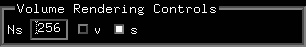
Ns: Volume Rendering Settings (use BHelp for details)
Set the number of slices used to render the volume. Volume rendering is done by slicing the volume from the far end along your vieweing direction to the front, blending successive images along the way. The more slices you use the better the result, something comparable to the maximum number of voxels in any of the directions would be a good start. Of course, the more slices, the slower the rendering.
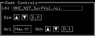
Label of dataset currently selected. Note that for some objects, like surfaces, what you’re viewing at any moment maybe a blend of multiple datasets. See color mixing for details.
Dim: Dimming factor to apply to colormap or color datasets.
Dimming factor to apply to colormap
before mapping the intensity (I) data.
The colormap, if displayed on the right,
is not visibly affected by Dim but the
colors mapped onto the surface, voxel grid, tracts, etc. are.
For RGB Dsets (e.g. .col files, or tract colors), Dim is
applied to the RGB colors directly.
Decreasing Dim is useful when the colors are too saturated
for lighting to reflect the object terrain.
When in doubt, just press the button and see what happens.
Avl: Choose method for computing color alpha value for voxels.
Choose the method for assigning an alpha value (A) to a voxel’s color.
Avg : A = average of R, G, B values
Max : A = maximum of R, G, B values
Min : A = minimum of R, G, B values
I : A is based on I selection. I range parameters apply
T : A is based on T selection. Full range is used.
B : A is based on B selection. B range parameters apply
Alpha threshold of Dset’s rendered slices.
When datasets’ voxels get colored, they get an Alpha (A) value
in addition to the R, G, B values. A is computed based on
the setting of the ‘Avl’ menu.
Voxels (or more precisely, their openGL realization)
with Alpha lower than this value will not get rendered.
This is another way to ‘threshold’ a rendered volume, and
is comparable to thresholding with the slider bar if using a
monochromatic increasingly monotonic colormap with ‘Avl’ set to
one of Max, Min, or Avg.
Note that thresholding with the slider bar sets A for thresholded
voxels to 0.0 regardless of the setting for ‘Avl’.
Thresholding with Ath is faster than using the slider bar because
it does not require recreating the whole texture.
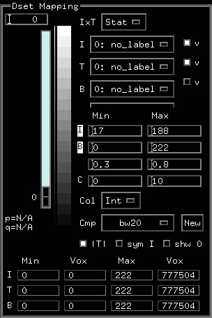
Use this menu to select which column (sub-brick) in the dataset (Dset) should be used for an Intensity (I)measure.
Values in (I) are the ones that get colored by the colormap,however, no coloring is done if the ‘v’ button on the right isturned off.
The (I) value for the selected datum (n) is shown in the ‘Val’ tableof the ‘Xhair Info’ section on the left.
The value is also shown in the SUMA viewer
You can use a different type of selector to set (I). A right-click on ‘I’ opens a list widget, which is better when you have many columns from which to choose.
The style of this selector can also change depending on the numberof sub-bricks (columns) you have in your dataset. If the numberexceeds a threshold specified by the environment variable SUMA_ArrowFieldSelectorTrigger
Thresholding is not applied when the ‘v’ button on the right is turned off.
The (T) value for the selected datum (n) is shown in the ‘Val’ tableof the ‘Xhair Info’ section on the left.
The value is also shown in the SUMA viewer
You can use a different type of selector to set (T). A right-click on ‘T’ opens a list widget, which is better when you have many columns from which to choose.
The style of this selector can also change depending on the number of sub-bricks (columns) you have in your dataset. If the number exceeds a threshold specified by the environment variable SUMA_ArrowFieldSelectorTrigger
Use this menu to select which column (sub-brick) in the dataset (Dset) should be used for color Brightness (B) modulation.
The (B) values are the ones used to control the brightness of a datum’s color.
Brightness modulation is controlled by ranges in the ‘B’ cells of the table below.
Brightness modulation is not applied when the ‘v’ button on
the right is turned off.
The (B) value for the selected datum (n) is shown in the ‘Val’ tableof the ‘Xhair Info’ section on the left.
The value is also shown in the SUMA viewer
You can use a different type of selector to set (B). A right-click on ‘B’ opens a list widget, which is better when you have many columns from which to choose.
The style of this selector can also change depending on the numberof sub-bricks (columns) you have in your dataset. If the numberexceeds a threshold specified by the environment variable SUMA_ArrowFieldSelectorTrigger
Colorbar used for colorizing values in ‘I’ sub-brick.
Colorization depends on the settings under the I, Range Setting, among other things. Threshold settings determine whether or not a certain value will get displayed at all.
Set threshold value to determine which nodes/voxels/edges will get coloredVoxels for which the value in the ‘T’ sub-brick is below that of the threshold will not get colored.
Used for setting the clipping ranges. Clipping is only done for
color mapping. Actual data
values do not change.
SetRangeTable.r01: Intensity clipping range (append ‘%’ for percentiles, see BHelp)
Intensity clipping range rules:
Values in the intensity data that are less than Min are colored by the first (bottom) color of the colormap.
Values larger than Max are mapped to the top color.
Intermediate values are mapped according to the ‘Col’ menu below.
You can set the range as a percentile of the dataset’s values by appending ‘%’ to the percentile for Min and/or Max such as 5% or 90%. Note that the percentile always gets replaced by the actual value in the dataset.
A left-click on ‘I’ locks ranges from automatic resetting, and the locked range applies to the current Dset only. A locked range is indicated with the reverse video mode.
A right-click resets values to the default range (usually 2% to 98%) in the dataset.
Values in the brightness (B) column are clipped to the Min to Max range in this row before calculating their modulation factor per the values in the next table row.
You can set the range as a percentile of the dataset’s values by appending ‘%’ to the percentile for Min and/or Max such as 8% or 75%. Note that the percentile always gets replaced by the actual value in the dataset.
A left-click locks ranges in this row from automatic resetting, and a locked range is applied to the current Dset only. A locked range is indicated with the reverse video mode.
A right-click resets values to the default range (usually 2% to 98%) for the dataset.
Brightness modulation factor range.
Brightness modulation values, after
clipping per the values in the row above,
are scaled to fit the range specified
here.
Switch between modes for mapping values to the color map.
The bottom color of the map C0 maps to the minimum value in the I range row, and the top color to the maximum value. Colors for values in between the minimum and maximum of I range, the following methods apply
Int: Interpolate linearly between colors in colormap to find color at
icol=((V-Vmin)/Vrange * Ncol)
NN : Use the nearest color in the colormap. The index into the colormap of Ncol colors is given by
icol=floor((V-Vmin)/Vrange * Ncol)
with icol clipped to the range 0 to Ncol-1
Dir: Use intensity values as indices into the colormap. In Dir mode, the intensity clipping range is of no use.
icol=floor(V) with clipping to the range 0 to Ncol-1
Switch between available color maps.
If the number of colormaps is too large
for the menu button, right click over
the ‘Cmp’ label and a chooser with a
slider bar will appear.
More help is available via
ctrl+h while mouse is over the
colormap.
Node index at minimum.
Right click in cell to
have crosshair jump to
node’s index.
Same as ‘ctrl+j’ or
an entry in the ‘Node’ cell
under Xhair Info block.
Node index at maximum.
Right click in cell to
have crosshair jump to
node’s index.
Same as ‘ctrl+j’ or
an entry in the ‘Node’ cell
under Xhair Info block.
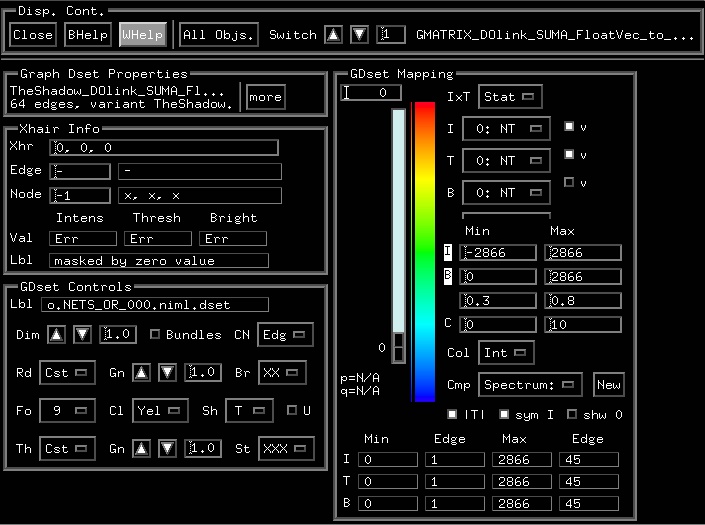
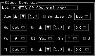
The graph controller is for controlling the way graphs (matrices) are rendered. Each graph gets its own controller. You can use the switch button above to switch between them. The graph controller is initialized by the graph of the last selected edge/cell.
After you have selected an edge, you can launch the Graph Controller with: ctrl+s or View‣Object Controller
Set/Get crosshair location in mm RAI on
this controller’s selected object.
Entering new coordinates
makes the crosshair jump
to that location (like ‘ctrl+j’).
Use ‘alt+l’ to center the
cross hair in your viewer.
1- Edge/Cell Index: Get/Set index of edge/cell in focus on this controller’s graph. This number is the 1D index of the edge/cell in the graph/matrix. Consider it the equivalent of a voxel 1D index in a volume, or a node in a surface dataset.
Entering a new edge’s index will put that edge in focus and send the crosshair to its center (like j). Use alt+l to center the cross hair in your viewer.
Note that an edge can be formed by a pair of identical nodes - think matrix diagonal.
2- Nodes Forming Directed Edge/Cell: For a cell, this would its pair of row and column indices into the matrix. For a graph, this would be the indices of the nodes forming the directed edge.
Data values at edge in focus. Intensity, Threshold, and Brightness show the triplets of values at the selected edge that correspond to the graph/matrix choices.in I, T, and B selectors.
Dim: Dimming factor to apply to colormap or color datasets.
Dimming factor to apply to colormap
before mapping the intensity (I) data.
The colormap, if displayed on the right,
is not visibly affected by Dim but the
colors mapped onto the surface, voxel grid, tracts, etc. are.
For RGB Dsets (e.g. .col files, or tract colors), Dim is
applied to the RGB colors directly.
Decreasing Dim is useful when the colors are too saturated
for lighting to reflect the object terrain.
When in doubt, just press the button and see what happens.
Bundles: Show bundles instead of edges if possible.
Show bundles instead of edges between nodes if
the graph dataset contains such information. For
the moment, only 3dProbTrackID creates such data.
Bundle colors reflect the value of the edge connecting the two nodes
Selection is identical to when edges are represented by straight lines.
CN: How to display connection to selected graph node.
When a node, rather than an edge is selected, choose how connections to it are displayed.
Edg: Show connections to selected node with edges, either straight lines or with bundles.
Col: Show connections to selected node by changing the colors of the connecting nodes, based on edge value. Edges are not displayed. the idea here is to reduce the clutter of the display, while still allowing you to visualize connection strength to one node at a time.
Rad: Show connections to selected node by changing the radius of the connecting nodes, based on edge value. Edges are not displayed in this mode also.
CaR: Both Col and Rad
XXX: Do nothing special, keep showing whole graph, even when selecting a graph node.
Use this menu to select which column (sub-brick) in the dataset (Dset) should be used for an Intensity (I)measure.
Values in (I) are the ones that get colored by the colormap,however, no coloring is done if the ‘v’ button on the right isturned off.
The (I) value for the selected datum (n) is shown in the ‘Val’ tableof the ‘Xhair Info’ section on the left.
The value is also shown in the SUMA viewer
You can use a different type of selector to set (I). A right-click on ‘I’ opens a list widget, which is better when you have many columns from which to choose.
The style of this selector can also change depending on the numberof sub-bricks (columns) you have in your dataset. If the numberexceeds a threshold specified by the environment variable SUMA_ArrowFieldSelectorTrigger
Thresholding is not applied when the ‘v’ button on the right is turned off.
The (T) value for the selected datum (n) is shown in the ‘Val’ tableof the ‘Xhair Info’ section on the left.
The value is also shown in the SUMA viewer
You can use a different type of selector to set (T). A right-click on ‘T’ opens a list widget, which is better when you have many columns from which to choose.
The style of this selector can also change depending on the number of sub-bricks (columns) you have in your dataset. If the number exceeds a threshold specified by the environment variable SUMA_ArrowFieldSelectorTrigger
Use this menu to select which column (sub-brick) in the dataset (Dset) should be used for color Brightness (B) modulation.
The (B) values are the ones used to control the brightness of a datum’s color.
Brightness modulation is controlled by ranges in the ‘B’ cells of the table below.
Brightness modulation is not applied when the ‘v’ button on
the right is turned off.
The (B) value for the selected datum (n) is shown in the ‘Val’ tableof the ‘Xhair Info’ section on the left.
The value is also shown in the SUMA viewer
You can use a different type of selector to set (B). A right-click on ‘B’ opens a list widget, which is better when you have many columns from which to choose.
The style of this selector can also change depending on the numberof sub-bricks (columns) you have in your dataset. If the numberexceeds a threshold specified by the environment variable SUMA_ArrowFieldSelectorTrigger
Colorbar used for colorizing values in ‘I’ sub-brick.
Colorization depends on the settings under the I, Range Setting, among other things. Threshold settings determine whether or not a certain value will get displayed at all.
Set threshold value to determine which nodes/voxels/edges will get coloredVoxels for which the value in the ‘T’ sub-brick is below that of the threshold will not get colored.
Used for setting the clipping ranges. Clipping is only done for
color mapping. Actual data
values do not change.
SetRangeTable.r01: Intensity clipping range (append ‘%’ for percentiles, see BHelp)
Intensity clipping range rules:
Values in the intensity data that are less than Min are colored by the first (bottom) color of the colormap.
Values larger than Max are mapped to the top color.
Intermediate values are mapped according to the ‘Col’ menu below.
You can set the range as a percentile of the dataset’s values by appending ‘%’ to the percentile for Min and/or Max such as 5% or 90%. Note that the percentile always gets replaced by the actual value in the dataset.
A left-click on ‘I’ locks ranges from automatic resetting, and the locked range applies to the current Dset only. A locked range is indicated with the reverse video mode.
A right-click resets values to the default range (usually 2% to 98%) in the dataset.
Values in the brightness (B) column are clipped to the Min to Max range in this row before calculating their modulation factor per the values in the next table row.
You can set the range as a percentile of the dataset’s values by appending ‘%’ to the percentile for Min and/or Max such as 8% or 75%. Note that the percentile always gets replaced by the actual value in the dataset.
A left-click locks ranges in this row from automatic resetting, and a locked range is applied to the current Dset only. A locked range is indicated with the reverse video mode.
A right-click resets values to the default range (usually 2% to 98%) for the dataset.
Brightness modulation factor range.
Brightness modulation values, after
clipping per the values in the row above,
are scaled to fit the range specified
here.
Switch between modes for mapping values to the color map.
The bottom color of the map C0 maps to the minimum value in the I range row, and the top color to the maximum value. Colors for values in between the minimum and maximum of I range, the following methods apply
Int: Interpolate linearly between colors in colormap to find color at
icol=((V-Vmin)/Vrange * Ncol)
NN : Use the nearest color in the colormap. The index into the colormap of Ncol colors is given by
icol=floor((V-Vmin)/Vrange * Ncol)
with icol clipped to the range 0 to Ncol-1
Dir: Use intensity values as indices into the colormap. In Dir mode, the intensity clipping range is of no use.
icol=floor(V) with clipping to the range 0 to Ncol-1
Switch between available color maps.
If the number of colormaps is too large
for the menu button, right click over
the ‘Cmp’ label and a chooser with a
slider bar will appear.
More help is available via
ctrl+h while mouse is over the
colormap.
Edge index at minimum.
Right click in cell to
have crosshair jump to
edge’s index.
Same as ‘ctrl+j’ or
an entry in the ‘Edge’ cell
under Xhair Info block.
Edge index at maximum.
Right click in cell to
have crosshair jump to
edge’s index.
Same as ‘ctrl+j’ or
an entry in the ‘Edge’ cell
under Xhair Info block.
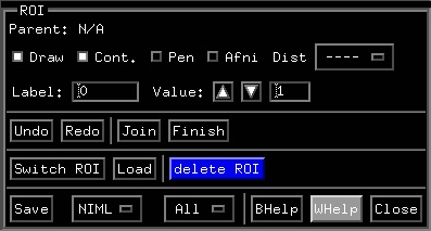
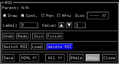
Toggles ROI drawing mode.
If turned on, then drawing is enabled
and the cursor changes to a target.
To draw, use the right mouse button.
If you want to pick a node without causing
a drawing action, use shift+right button.
After the draw ROI window is open, you can toggle
this button via ctrl+d also.
Toggles Pen drawing mode
If turned on, the cursor changes shape to a pen.
In the pen mode, drawing is done with button 1.
This is for coherence with AFNI’s pen drawing mode,
which is meant to work pleasantly with a stylus directly
on the screen. In pen mode, you draw with the left mouse
button and move the surface with the right button.
To pick a node, use shift+left button.
Pen mode only works when Draw Mode is enabled.
Toggles Afni Link for ROI drawing.
If turned on, then ROIs drawn on the surface are
sent to AFNI.
Surface ROIs that are sent to AFNI are turned
into volume ROIs (VOIs) on the fly and displayed
in a functional volume with the same colormap used in SUMA.
The mapping from the surface domain (ROI) to the volume
domain (VOI) is done by intersection of the first with
the latter. The volume used for the VOI has the same
resolution (grid) as the Surface Volume (-sv option)
used when launching SUMA. The color map used for ROIs
is set by the environment variable SUMA_ROIColorMap.
trace: Calculate distance along last traced segment.
all: In addition to output from ‘trace’, calculate the shortest distance between the first and last node of the trace.
The results are output to the Message Log window (Help –> Message Log) with the following information:
n0, n1: Indices of first and last node forming the traced path.
N_n: Number of nodes forming the trace.
lt: Trace length calculated as the sum of the distances from node to node. This length is a slight overestimation of the geodesic length. Units for all distances is the same as the units for surface coordinates. Usually and hopefully in mm.
lt_c: Trace length corrected by a scaling factor from [1] to better approximate geodesic distances. Factor is 2/(1+sqrt(2)). Do not use this factor when N_n is small. Think of the extreme case when N_n is 2.
sd: Shortest distance on the mesh (graph) between n0 and n1 using Dijkstra’s algorithm.
sd_c: Corrected shortest distance as for lt_c.
Note 1: sd and sd_c take some time to compute. That is why they are only calculated when you select ‘all’.
Note 2: The output is formatted to be cut and pasted into a .1D file for ease of processing. You can include all the comment lines that start with ‘#’. But you cannot combine entries from the output obtained using ‘all’ option with those from ‘trace’ since they produce different numbers of values.
Label of ROI being drawn.
It is very advisable that you use
different labels for different ROIs.
If you don’t, you won’t be able to
differentiate between them afterwards.
Join the first node of the ROI to the last,
thereby creating a close contour ROI.
This is a necessary step before the filling
operation. Joining is done by cutting the surface
with a plane formed by the two nodes
and the projection of the center of your window.
You could double click at the last node, if you don’t
want to use the ‘Join’ button.
Mark ROI as finished.
Allows you to start drawing a new one.
Once marked as finished, an ROI’s label
and value can no longer be changed.
To do so, you will need to ‘Undo’ the
finish action.
Save the Drawn ROI to disk.
Choose the file format and what is to be
saved from the two menus ahead.
File format for saving ROI:
Format options are 1D and NIML.
The 1D format is the same one used in AFNI.
It is an ASCII file with 2 values per line. The first
value is a node index, the second is the node’s value.
Needless, to say, this format does not support the storage
of ROI auxiliary information such as Label and
Parent Surface, etc., nor does it preserve the order in which
nodes are traversed during a tracing. For that you’ll have to use :term:NIML.
NIML is a whole different story which will be documented
(if necessary) in the future. Suffice it to say that in NIML
format you can store all the auxiliary information about
each ROI, unlike with the .1D format.
But more importantly, the NIML format allows you to preserve the order in which you traced the ROI. You can actually use
Undo/ref:Undo<ROICont->ROI->Redo> on ROIs save in NIML format.This information can be later used for the purpose of sampling
cortical activity along a particular path. This would be accomplished
with the aid of ROI2dataset’s -nodelist* options, along with
ConvertDset’s -node_select_1D option.
Which ROIs to save?
This: saves the current ROI.
All: saves all ROIs on surfaces related to the Parent surface of the current ROI.