7.3. @GradFlipTest: checking on gradient flips

Warning

This is an annoying feature of DWI/DTI processing. Probably my least favorite aspect. But it’s also quite important to understand and deal with (hopefully just once at the beginning of a study).

7.3.1. Overview

	Mathematical points about tensors and their scalar and vector properties.
Point I:	Mathematically, there are a lot of symmetries in the diffusion tensor model (and also in HARDI ones, for that matter). A consequence of this is that using a gradient, , or its negative, , makes absolutely no difference in the model fitting– the resulting tensor will look the same. (NB: this equanimity is not referring to twice refocused spin-echo EPI or any sequence features– purely to post-acquisition analysis.)
Point II:	The above symmetry does not quite apply in the case that not all components are simultaneously flipped. If just one or two are, then the scalar parameter values of the tensor will be the same (i.e., things that describe magnitudes, such as FA, MD, RD, L1, L2 and L3), but some of the vector parameters (i.e., the eigenvectors V1, V2 and V3 that describe the orientation orientation) can/will differ. So, if one fits using a gradient and then with another related one , then the two fits would have the same scalar parameters (, etc.) but different vectors (, etc.).
Point III:	Any two flips leads to equivalent fitting by just flipping the third gradient (due to the symmetries described above in Points I and II). Thus, using the gradient or would lead to the same tensor fit.
Point IV:	The scanner has its own set of coordinate axes, and this determines each dataset’s origin and orientation (all of which can by reading the file’s header information, e.g., 3dinfo -o3 -orient FILE). The scanner axes also determine the values of the DW gradient/matrix components, both their magnitude and sign.

The problem at hand: for some unbeknownst reason, the way gradients are stored in dicoms (and subsequent file formats such as NIFTI, etc.) there may be a systematic sign change in the recorded gradient components, relative to how a software interprets them. The problem takes the following form: a single component of each gradient appears to have had its sign flipped in the output file (always the same gradient per file): for example, .

This is quite an annoying thing to have happen. Furthermore, it appears to be dependent as well on the programs used (they often have separate conventions; for all AFNI functions it should be the same, but it might be different for TORTOISE or other programs (but we don’t care about other-other programs, anyways, at least)).

Some of the good news:

• it is pretty straightforward to determine when gradients and data are ‘unmatched’ (see the next section and the purdy pictures therein);

• there’s something that can be done to fix the problem, relatively simply; and

• usually, once you determine the fix for one subject’s data set, the rest of the data from the same scanner+protocol follows suit. Usually.

7.3.2. Picturing the effect of flipping

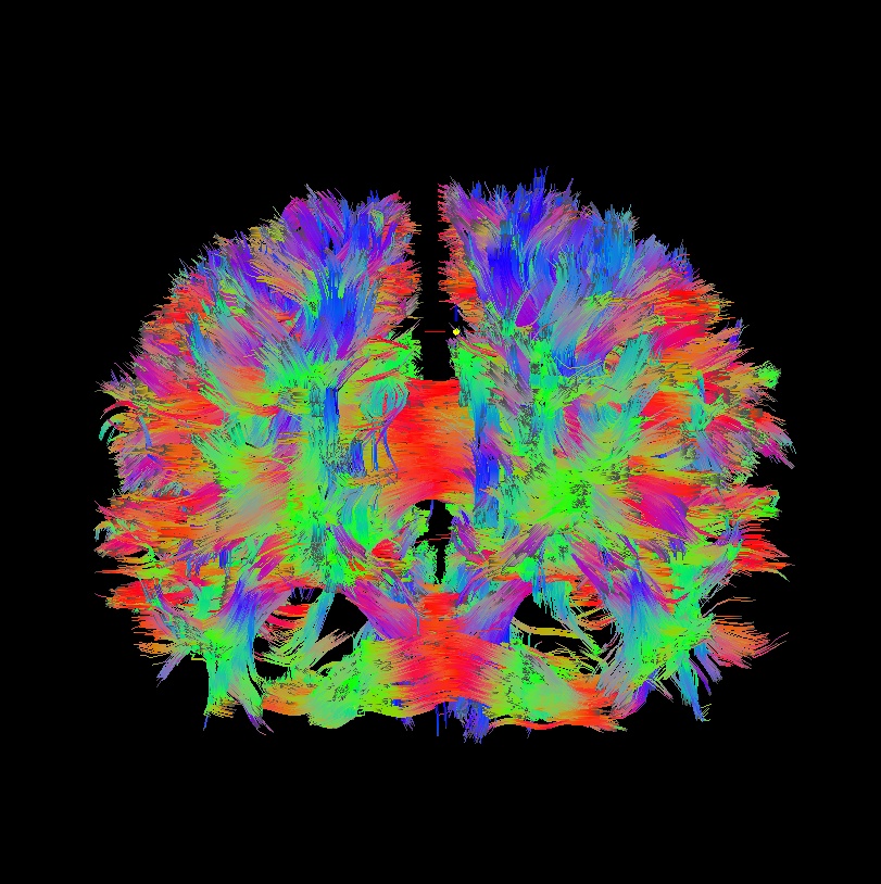
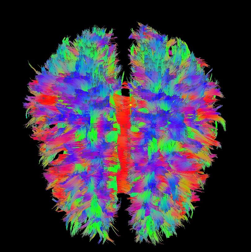
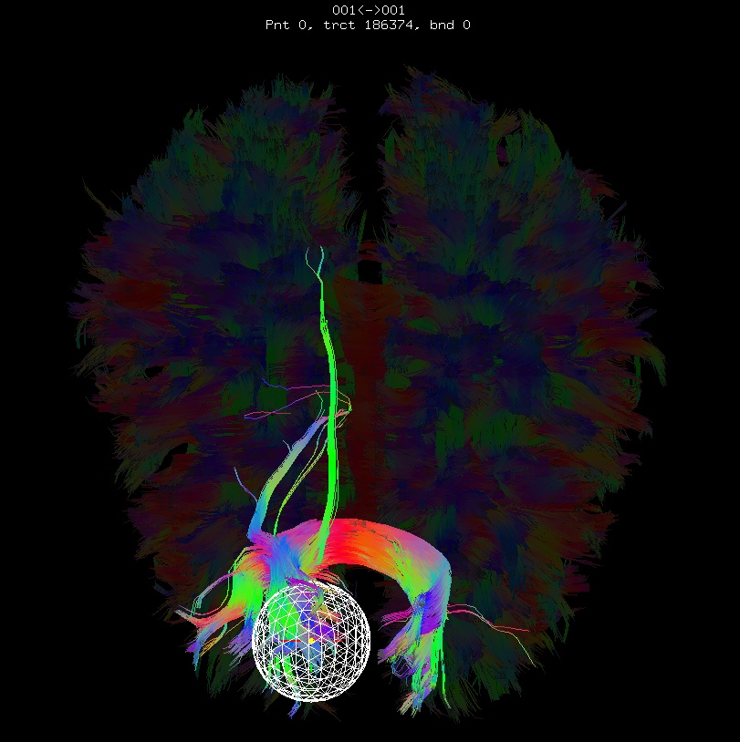
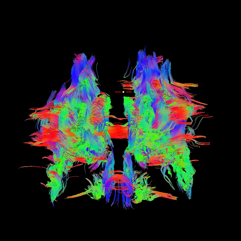
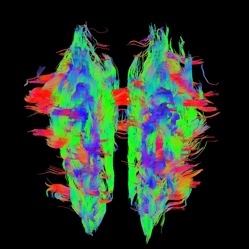
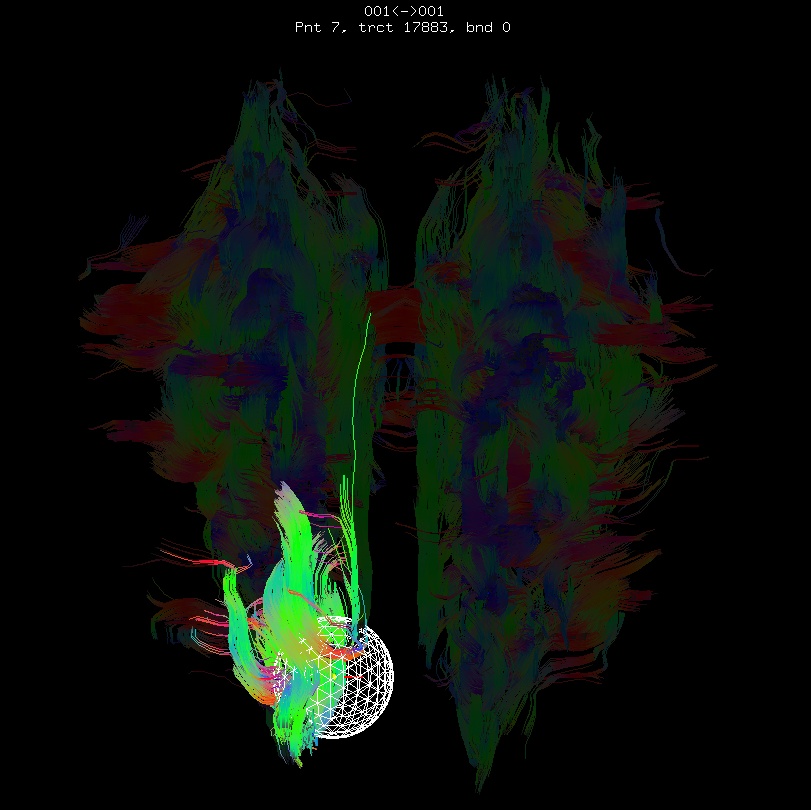
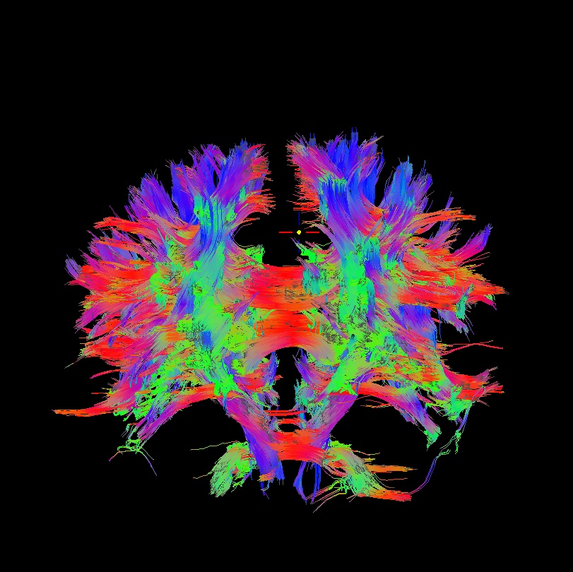
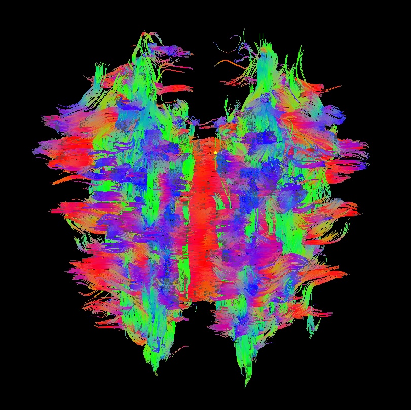
For me it is difficult to view eigenvector maps and know what’s going on, so I use a quick, whole brain (WB) tractography as a way to see that things have gone wrong. The premise is that, since the directionality of most DTs will be wrong, the most basic WM features of the brain, such as the corpus callosum, will not look correct (NB: if you are working with subjects whose transcallosal fibers may be highly nonstandard, I suggest using a control subject for checking about gradient flips).

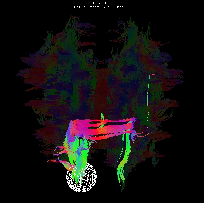
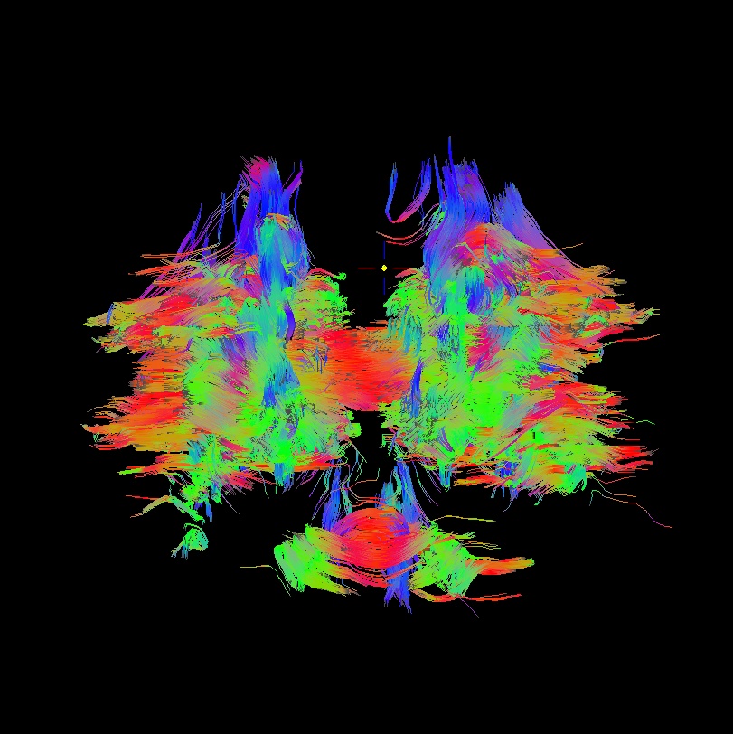
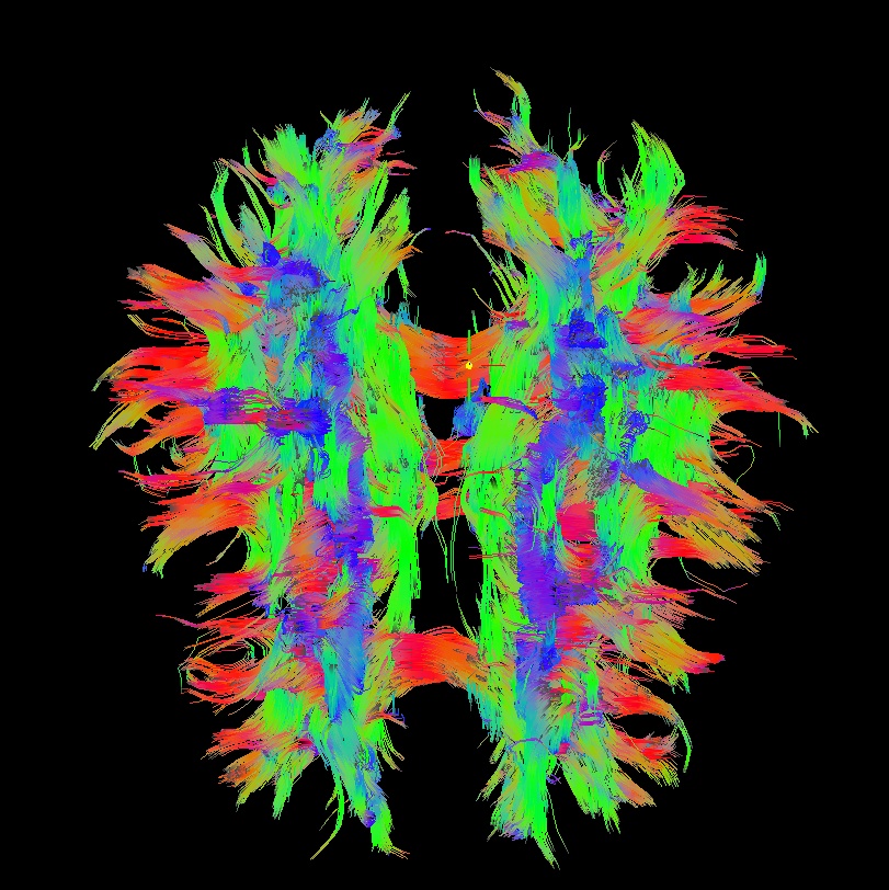
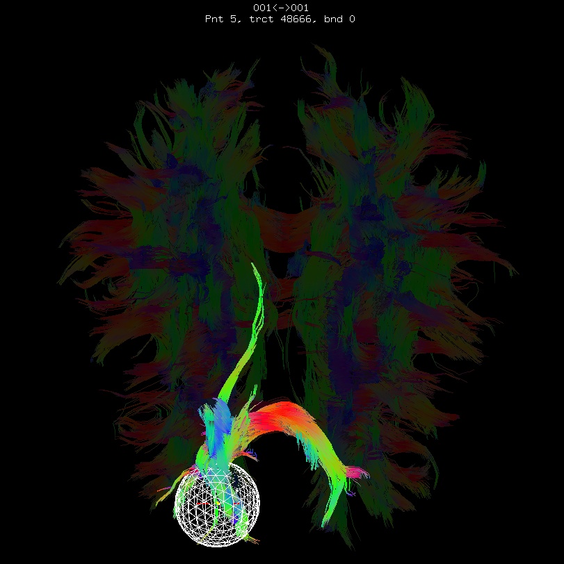
Below are sets of images from (bad) data in need of each potential kind of flip, as well as a (good) data which has been properly flipped. From left to right, columns show the following tractographic views of the same data set: fronto-coronal WB; supero-axial WB; supero-axial ROI (spherical mask located in the genu and anterior cingulum bundle):

good: no relative flip

bad: flipped x

bad: flipped y

bad: flipped z

As seen above, several of the badly flipped sets have (among other detrimental features) variously missing corpus callosum/genu/splenium/cingulate tracts, poor WB coverage, and oddly spiking (blue) tracts in the superior region (known as the bad hair day effect). In practice, the y-flip might be the least obvious to detect at first glance, but several features are different– for instance, the genu and splenium are missing. The badly flipped images are in contrast with the nice, full quasi-cauliflower that is the well flipped set in the top row.

7.3.3. Using @GradFlipTest

The Question: How do you know what is the correct flip for your data?

The Answer: Check how the whole-brain tracking looks for each of the four possibilities: x-flip, y-flip, z-flip and none. Whichever one is clearly the best is correct. (And yes, there should be a clear winner– if not, one might have to look at other things, like DICOM conversion, etc.)

The Function: In order to provide “The Answer” (or at least “an” answer), @GradFlipTest exists to automatically perform all of the whole brain tracking tests and count up the results; it even helps users look at results for additional verification. One provides @GradFlipTest with the DWIs + gradient information, and then:

• tensors are fit

• tracking is performed with each possible flip (x, y, z and none)

• numbers of long tracts is calculated

• and based on the relative numbers of tracts, there should be a clear winner from the possible options

• users are prompted to look at the results with suma commands that are displayed in the terminal

• the best guess is dumped into a file, for scriptability.

Once the correct flip is known, one can put this information into 1dDW_Grad_o_Mat++ (or even some of the newer fat_proc* functions described in the tutorial pages, “FATCAT: DWI {Pre-pre-, Pre-, Post-pre}processing”), which contains switches to flip each component (even if one is using matrix formats instead of gradients, these apply): -flip_x, -flip_y, and -flip_z (default is just “no flip”, but there actually is an explicit option for this, -no_flip, which might seem useless but actually makes scripting easier).

Note

Anecdotally, it seems that data from Siemens scanners often requires a -flip_y when brought into AFNI. However, it is always worth checking for yourself at the start of a study.

Note

At present, DWIs processed using TORTOISE v3.0 seem to often require a -flip_z when brought into AFNI. However, always check for yourself!.

Example commands:

• This is an example of taking a DWI dset (“buddi.nii”) and a TORTOISE-style b*-matrix (“buddi.bmtxt”) after running their DR_BUDDI program, and testing for flips:

  @GradFlipTest                           \
      -in_dwi       buddi.nii               \
      -in_col_matT  buddi.bmtxt             \
      -prefix       GradFlipTest_rec.txt
  

-> This puts results into the same directory with the “buddi.*” files (because that there is no separate path as part of the -prefix *), and the outputs are:

Directory substructure for example data set
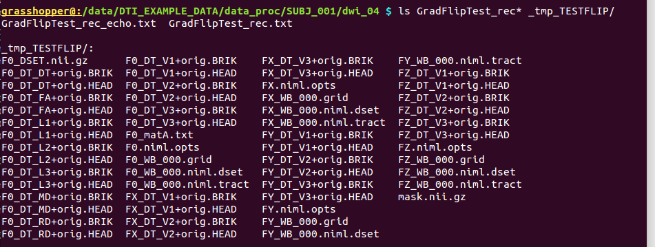
Output text files (“Grad*”) and temporary subdirectory made by @GradFlipTest.

Outputs of	@GradFlipTest
GradFlipTest_rec.txt	textfile, simply the “recommended” option based on tracking results– can be echoed into command calls to 1dDW_Grad_o_Mat++ (but user should be sure that the chosen winner is really so!).
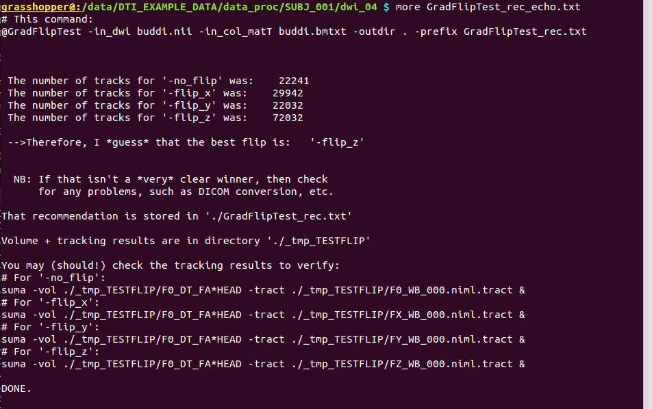
GradFlipTest_rec_echo.txt	textfile, with copy of the command that was run, and more verbose output, such as the tract counts, as well as example commands for viewing all results in SUMA.
_tmp_TESTFLIP/	a working directory of tensor fits and intermediate files, as well as the tracking results for all flips, which can (should be!) viewed to doublecheck results.

The text file outputs, GradFlipTest_rec*txt (here, echoed to terminal)

7.3.4. Combining with 1dDW_Grad_o_Mat++ (or fat_proc functions)

Since the recommended output flip is stored by itself in a text file, that text file can be echoed into a variable and then entered into other commands, such as 1dDW_Grad_o_Mat++ or some of the fat_proc functions like fat_proc_dwi_to_dt (and others). That means that @GradFlipTest can be inserted into pipelines fairly straightforwardly.

For example, one could combine the above command with 1dDW_Grad_o_Mat++:

# guesstimate flip
@GradFlipTest                           \
    -in_dwi       buddi.nii               \
    -in_col_matT  buddi.bmtxt             \
    -prefix       GradFlipTest_rec.txt

# echo the flip value into a file
set my_flip = `cat GradFlipTest_rec.txt`

# apply that flip when converting matrices
1dDW_Grad_o_Mat++                        \
    -in_col_matT  buddi.bmtxt            \
    -out_col_matA dwi_matA.txt           \
    $my_flip

-> note that this even works if the recommendation were not to flip at all, because the text file who hold the flag -no_flip, which is a permissible argument to 1dDW_Grad_o_Mat++.

But see the caution on over-exuberance in scripting (and not checking the @GradFlipTest results by eye) below.

7.3.5. Caveats with @GradFlipTest

It is important to note that @GradFlipTest takes a best guess at the recommendable flip– it isn’t always right. The first sign of badness is typically when there is not a very clear winner in the tract counting– the winning value should probably be 2-3 times each of the others, at least.

Things that can go wrong include:

• poor automasking of the data set, perhaps due to severe brightness inhomogeneities (-> you can make a separate mask and enter it as an option);

• gradient tables not matching data, for example due to problems with how the gradients were stored in the DICOM headers or with how they were converted (-> you can try to get the grad information directly from your scanner);

• having inappropriate tracking parameters set, such as FA threshold or minimum tract length (-> defaults are set for mainly-healthy adult humans– if your set is otherwise, change these appropriately);

• noisy, bad or corrupted data (-> ummm, back to the drawing board on this one perhaps– can’t work a miracle; but perhaps something can be done?).

The biggest problem I have seen is gradient tables not matching data– beware odd ways data have been stored or written or miscopied, etc.