12.18.1. Basic meta analysis with BML

Introduction

Here we provide the data and code for the basic meta analysis example with Bayesian multilevel modeling (BML) presented in Sec. 3.1 of *link to bioRxiv paper* (see Fig. 5 there).

BML meta analysis

The data

The data for this example is stored in a simple text file, formatted like this:

 Study     ef     se
     1   0.62   0.23
     2   0.76   0.54
     3   0.23   0.46
     4   0.49   0.38
     5   0.92   0.28
     6   0.62   0.45
     7   0.51   0.48
     8   0.79   0.21
     9   0.82   0.45
    10  -0.14   0.59
    11   0.27   0.36

Download data: data_meta1.txt

The three columns contain, respectively: a study index, effect estimate (ef) and standard error (se).

The script

The R language code for performing the meta analysis and making a simple plot of the results is as follows:

# Read input and load libraries                  
dat <- read.table('data_meta1.txt', header=T)  
library(brms,BH)                                 
                                                 
# Set and run 4 chains                           
options(mc.cores = parallel::detectCores())      
fm <- brm(ef | se(se, sigma=FALSE) ~ 1+(1|Study),
          data=dat, chains = 4, iter=1000)       
                                                 
# Simple output display                          
plot(density(fixef(fm, summary = FALSE)),        
     xlim=c(-0.2,1.2))                           
abline(v=0, col="green3")                        

Download data: run_meta1.R

The program loads the input data file and libraries, and then runs the BML model with 4 parallel chains, and finally plots the resulting effect estimate distribution.

The output

This displays the estimated posterior distribution for the effect estimate:

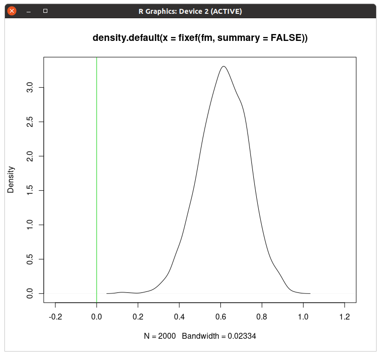
The vertical green line shows the zero effect. In this case, the vast majority of the distribution is to the right of this zero effect line, which is interpreted as strong evidence for having a positive effect.

(See the paper for more details.)

Welcome to Bayesian analysis! It’s not so bad, is it?