You can download the set of scripts and supplementary files for
running this demo here:
The scripts for this demo are also shown one-by-one below, so one can
read along with them.
The scripts are meant to be run in the AFNI_demos/FATCAT_DEMO
directory. Alternatively, you could copy out the following files
(which are all that are used from there) and make a new directory:
- mprage+orig
a standard anatomical volume (T1w, with skull)
- errts.anaticor.FATCAT+orig
an EPI time series data set, approximately aligned to the
mprage+orig dset
Additional files provided here include:
- 00_input_keys_values.txt
a text file with two columns: 1) integer values, and 2) string
labels. There is one integer value plus string label pair for
each ROI (5 total).
- 00_list_of_all_roi_centers.txt
a list of (x, y, z) coordinates (in RAI orientation)
The do_00_setup_example.tcsh script will actually create the ROIs
for this tutorial, so that we all have the same starter ROI masks
(using the locations specified in the “00_list*.txt” file).
Additionally, this setup script makes a skull-stripped version of the
anatomical volume, mainly for defining a focused region within which
to select slices to view with @chauffeur_afni.
This first step is just to create some additional files that we will
need (the set of ROIs) and want (a skull-stripped
anatomical) for the demo.
- show code y/n -
#!/bin/tcsh

# =================================================================
# do_00_setup_example.tcsh
#
# Precursor script simply to generate *some* set of ROI files, which
# will then be combined into a single map using the other scripts
# here.  Usually, the user would have their own already defined in
# some meaningful manner.
#
# The only condition on the ROIs here is that they *don't* overlap
# spatially.  While the other program can be designed with a minor
# change to deal with that situation, here we assume that overlap
# would be an unwanted thing and a sign of a mistake in processing, so
# it is in fact guarded against in the other scripts.
#
# This script also makes a skull-stripped version of the anatomical,
# for use in defining a brain-specific volume to snapshot over.
#
# ver  : 1.0
# date : Nov. 19, 2018
# auth : PA Taylor (NIMH, NIH)
# =================================================================

# input files-- needed in directory
set ilist    = 00_list_of_all_roi_centers.txt
set vepi     = errts.anaticor.FATCAT+orig
set vanat    = mprage+orig
set vanatss  = mprage_ss.nii.gz

# outputs/temp files
set opref    = roi_mask
set tlist    = _tmp_roi_list.txt

# -----------------------------------------------------------

# Get number of cols in ROI list- Ncol is Nrois
set dims = `1d_tool.py              \
                -show_rows_cols     \
                -verb 0             \
                -infile "${ilist}"`

# Need to know

foreach ii ( `seq 1 1 ${dims[1]}` )
    set iii = `printf "%03d" ${ii}`

    # make temp list of 1 ROI center
    sed -n ${ii}p ${ilist} > ${tlist}

    # make a volumetric mask of a sphere at that center; the sphere
    # locations were chosen using InstaCorr in AFNI GUI, and so were
    # specified as RAI values
    3dUndump                              \
        -overwrite                        \
        -xyz                              \
        -orient RAI                       \
        -prefix ${opref}_${iii}.nii.gz    \
        -master ${vepi}                   \
        -datum byte                       \
        -srad 9.5                         \
        ${tlist}

end

echo "++ Skull-stripping the anat vol."
3dSkullStrip                             \
    -orig_vol                            \
    -input ${vanat}                      \
    -prefix ${vanatss}

# clean up
\rm ${tlist}

# and done
echo "++ DONE!"
exit 0
Notable outputs of |
do_00*.tcsh
|
|---|
roi_mask_*.nii.gz |
set of dsets, each a mask of an ROI (here, just a spherical ball) |
mprage_ss.nii.gz |
a skull-stripped version of the anatomical (to be used during
the @chauffeur_afni stages, to make a “focus box” within
which slice range we will make auto-images) |
Combine a bunch of ROI masks (volumetric ones in separate, 3D vols)
into a single map of ROIs, where each one is comprised of voxels of
a constant integer value: first ROI file in list gets 1s, next ROI
file gets 2s, etc.
Each ROI will also get a string label – we assume the user has a text
file of string ‘values’ to match the ROI integer ‘keys’. That is, a
list of text names that follow the same order of ROI files.
- show code y/n -
#!/bin/tcsh

# =================================================================
# do_01_make_single_roi_map.tcsh
#
# Combine a bunch of ROI masks (volumetric ones in separate, 3D vols)
# into a single *map* of ROIs, where each one is comprised of voxels
# of a constant integer value: first ROI file in list gets 1s, next
# ROI file gets 2s, etc.
#
# Each ROI will also get a string label -- we assume the user has a
# text file of string 'values' to match the ROI integer 'keys'.  That
# is, a list of text names that follow the same order of ROI files.
#
# ver  : 1.0
# date : Nov. 19, 2018
# auth : PA Taylor (NIMH, NIH)
# =================================================================

# ------------- input files: needed in directory ---------------

set vepi     = errts.anaticor.FATCAT+orig
set vanat    = mprage+orig
set vanatss  = mprage_ss.nii.gz

# List of initial N ROI files to be combined. Each dset here should be
# a binary mask, with voxel values only 0 or 1
set irois    = `\ls roi_mask*gz`

# File of label+key values. Here, for N ROIs, the "keys" are integers,
# 1..N.  The order of labels should match the order of listing ${irois}
set ilabtxt  = 00_input_keys_values.txt

# ---------- output and supplementary files: made here ----------

# output ROI map volume
set opref     = final_roi_map
set omap      = ${opref}.nii.gz
set olt       = ${opref}.niml.lt

# temp files: made, then cleaned
set tpref    = _tmp
set tsum     = ${tpref}_0_roi_sum.nii.gz
set tcat     = ${tpref}_1_roi_cat.nii.gz

# -----------------------------------------------------------

# Add up all ROI masks.  This has two purposes:
# 1) We will check this for overlaps of ROIs (which would likely be bad).
# 2) We will use this as a mask in combining the ROIs
3dMean                           \
    -sum                         \
    -prefix "${tsum}"            \
    ${irois}

# ------------- Check if there is ROI overlap --------------------

# is max($tsum) > 1?
set sum_max = `3dinfo -dmax "${tsum}"`

if ( ${sum_max} > 1 ) then
    echo "** ERROR! overlapping ROI masks."
    exit 1
else
    echo "++ OK: ROI masks don't appear to overlap"
endif

# ------------- Glue to 4D dset --------------------

# concatenate in order of 'ls'
3dTcat                       \
    -prefix ${tcat}          \
    ${irois}

# ------------- Make 3D ROI map --------------------

# Give each ROI a different integer: the ROI voxels in [0]th brick
# each get a value of 1, and, generally, those in the [i]th brick get
# get a value of i+1.
3dTstat                      \
    -argmax1                 \
    -mask   ${tsum}          \
    -prefix ${omap}          \
    ${tcat}

# ------------- Attach labeltable --------------------

# Provide a list of key values (i.e., the integer of each ROI) and
# each (string) label to attach.  We specify which column is which in
# the file, and ... that's about it:
@MakeLabelTable                  \
    -lab_file   ${ilabtxt} 1 0   \
    -labeltable ${olt}           \
    -dset       ${omap}

# ------------- Make QC images --------------------

@chauffeur_afni                             \
    -ulay  ${vanat}                         \
    -olay  ${omap}                          \
    -box_focus_slices ${vanatss}            \
    -cbar ROI_i32                           \
    -func_range 32                          \
    -pbar_posonly                           \
    -opacity 9                              \
    -blowup 1                               \
    -save_ftype JPEG                        \
    -prefix   "${opref}"                    \
    -montx 6 -monty 3                       \
    -set_xhairs OFF                         \
    -label_mode 1 -label_size 3             \
    -do_clean

# ------------------ clean up --------------------------

\rm ${tpref}*


echo "++ DONE!"
exit 0
Notable outputs of |
do_01*.tcsh
|
|---|
final_roi_map.nii.gz |
single 3D volume containing all ROIs, and each ROI having its
own integer value as well as a string label attached |
final_roi_map.niml.lt |
the labeltable that is attached to “final_roi_map.nii.gz”;
shows what integer values are associated with what string
labels |
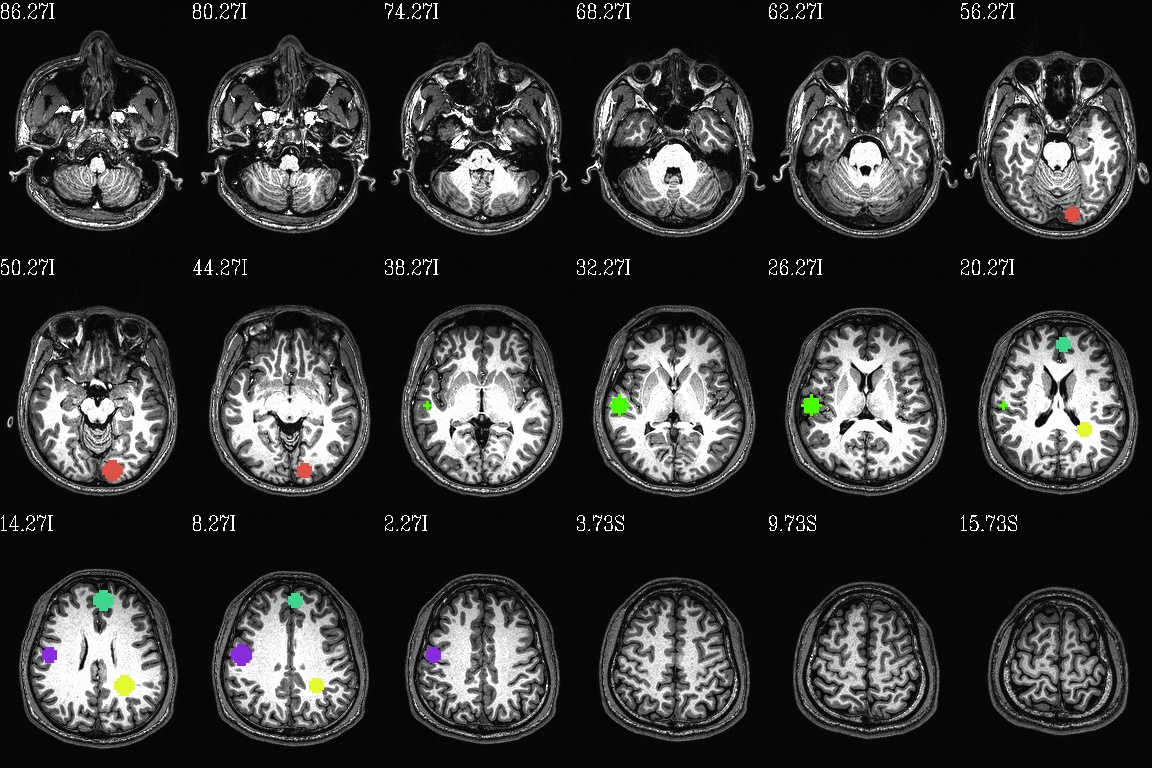
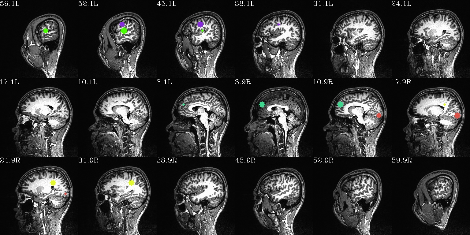
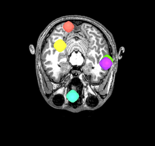
final_roi_map.*.jpg |
helpful QC images made to show a lot of slices across each
viewplane (axi, cor, sag) of the brain |
Some autoimages of do_01*.tcsh |
|---|
final_roi_map.axi.jpg: axial slices evenly spaced
throughout the brain region; there are 5 ROIs in total (note
the slightly hard to see yellow one in the WM) |
|
final_roi_map.sag.jpg: same as above, but sagittal views |
|
Basic example of turning volumetric ROIs into surfaces to view in
SUMA.
No images are made automatically here, but SUMA is opened for an
interactive view of the ROIs in the brain.
- show code y/n -
#!/bin/tcsh
#
# =================================================================
# do_02_surfaceize_rois.tcsh

# Basic example of turning volumetric ROIs into surfaces to view in
# SUMA.
#
# ver  : 1.0
# date : Nov. 19, 2018
# auth : PA Taylor (NIMH, NIH)
# =================================================================

# ------------- input files: needed in directory ---------------

set vepi     = errts.anaticor.FATCAT+orig
set vanat    = mprage+orig
set vanatss  = mprage_ss.nii.gz

# output ROI map volume
set opref    = final_roi_map
set omap     = ${opref}.nii.gz
set olt      = ${opref}.niml.lt
set ogii     = ${opref}.SURF

# Isosurface parameters
set tsmoo_kpb  = 0.01              # polishing level
set tsmoo_nit  = 6                 # number of iterations
set iso_choice = "isorois+dsets"   # mode: what to do
set merge_lab  = ""                # set depending on mode

# ------------- process: make some surfaces ---------------

if ( "${iso_choice}" == "mergerois" ) then
    set merge_lab = "${opref}"
endif

IsoSurface                              \
    -${iso_choice}   ${merge_lab}       \
    -input ${omap}                      \
    -o_gii ${ogii}                      \
    -Tsmooth ${tsmoo_kpb} ${tsmoo_nit}


# view with SUMA
suma                       \
    -onestate              \
    -i ${ogii}*.gii        \
    -vol ${vanat}

echo "++ DONE!"
exit 0
Notable outputs of |
do_02*.tcsh
|
|---|
final_roi_map.SURF.*.gii |
SUMA-able surface for each ROI |
final_roi_map.SURF.*.niml.dset |
set of label files, one for each *.gii surface |
New data files are not created here, but an example of “driving” SUMA
from the command line is presented. In this manner, we can move the
brain around in useful ways (i.e., to show standard viewplanes) and
automatically save images of those views. The images are saved in a
subfolder, with a user-specifiable prefix and time stamps combined in
each image file’s name.
On a local system, this should run fairly straightforwardly– though
note that the sleep commands, which do slow the process down by a
couple seconds, are necessary to allow the operations to stay orderly.
If this were run on a bigger, more detailed data set, longer sleep
commands might be necessary, but that would be very dependent on the
computer, memory specs, data set, etc.
Finally, note that the suma GUI must be able to open up on
screen for this to happen (so running this particular on a remote
system might be difficult, and/or you might have to log in with
ssh -X ... or something to be able to allow that to happen).
- show code y/n -
#!/bin/tcsh

# =================================================================
# do_03_drivesuma_views.tcsh
#
# Basic example of driving SUMA to view surfacized results and to save
# snapshots of planar views automatically.
#
# Resulting images get saved to a subdirectory.
#
# ver  : 1.0
# date : Nov. 19, 2018
# auth : PA Taylor (NIMH, NIH)
# =================================================================

# ------------- input files: needed in directory ---------------

set vepi     = errts.anaticor.FATCAT+orig
set vanat    = mprage+orig
set vanatss  = mprage_ss.nii.gz

# output ROI map volume
set opref     = final_roi_map
set omap      = ${opref}.nii.gz
set olt       = ${opref}.niml.lt
set ogii      = ${opref}.SURF
set here      = ${PWD}

# -------------------- image file parameters -----------------------

# Saved image naming props: directory and file prefix (latter, taken
# from olay filename here)
set image_dir = "$here/MY_ROI_SURF_IMAGES"
set image_pre = ${opref}

# size of the image window (bigger -> higher res), given as:
#       leftcorner_X  leftcorner_Y  windowwidth_X  windowwith_Y
setenv SUMA_Position_Original "50 50 500 500" #"50 50 3500 3500"

# --------------------- preliminary settings -----------------------

# boring stuff.
setenv SUMA_DriveSumaMaxCloseWait  20
setenv SUMA_DriveSumaMaxWait       10
setenv SUMA_AutoRecordPrefix       "${image_dir}/${image_pre}"
#setenv SUMA_SnapshotOverSampling $OVERSAMP

# port number for AFNI-SUMA talking, here just used so we can close
# SUMA automatically when finished with making images
set portnum = `afni -available_npb_quiet`

# ========================= run SUMA ============================

# --------------------- SUMA setup------------------------------

# view with SUMA
suma                       \
    -echo_edu              \
    -npb ${portnum}        \
    -onestate              \
    -i ${ogii}*.gii        \
    -vol ${vanat} &

echo "++ sleepy time..."
sleep 3

# for Macness
DriveSuma                                            \
    -echo_edu                                        \
    -npb ${portnum}                                  \
    -com surf_cont -view_surf_cont y

echo "++ more sleepy time..."
sleep 2

# In order, turn *OFF* visibility of the:
#    crosshair, selector node, selector faceset, and label
DriveSuma                                              \
    -echo_edu                                          \
    -npb ${portnum}                                    \
    -com viewer_cont -key 'F3' -key 'F4' -key 'F5' -key 'F9'

# Sagittal profile,  SNAP
DriveSuma                                              \
    -npb ${portnum}                                    \
    -com viewer_cont -key 'Ctrl+left'                  \
    -com viewer_cont -key 'Ctrl+r'

sleep 1

# same hemi, SNAP
DriveSuma                                              \
    -npb ${portnum}                                    \
    -com viewer_cont -key 'Ctrl+right'                 \
    -com viewer_cont -key 'Ctrl+r'

sleep 1

# front cor profile, SNAP
DriveSuma                                              \
    -npb ${portnum}                                    \
    -com viewer_cont -key 'Ctrl+up'                    \
    -com viewer_cont -key 'Ctrl+r'

sleep 1

# back cor profile, SNAP
DriveSuma                                              \
    -npb ${portnum}                                    \
    -com viewer_cont -key 'Ctrl+down'                  \
    -com viewer_cont -key 'Ctrl+r'

# Close SUMA running on the specified port number; could be commented
# out, if one wants SUMA to remain open
@Quiet_Talkers -npb_val ${portnum}

echo "++ DONE!"
exit 0
Notable outputs of |
do_03*.tcsh
|
|---|
MY_ROI_SURF_IMAGES/ |
sub-directory that will hold all images |
final_roi_map.A.*jpg |
image files in the “MY_ROI_SURF_IMAGES/” directory |
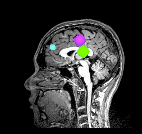
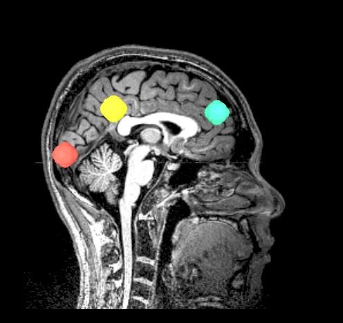
Some autoimages of do_03*.tcsh |
|
|---|
final_roi_map.A.181127_135159.989.jpg |
final_roi_map.A.181127_135201.103.jpg |
|
|
final_roi_map.A.181127_135202.220.jpg |
final_roi_map.A.181127_135203.346.jpg |
|
|
Example of using 3dNetCorr generate a correlation matrix for a set
of ROIs from time series averages; we also calculate WB seed-based
correlation maps of each ROI (for free!). It will be a good reminder
of how noisy each individual subject’s data set is…
Additionally, the correlation matrix from 3dNetCorr is also
JPG-ized.
- show code y/n -
#!/bin/tcsh
# =================================================================
# do_04_netcorr.tcsh
#
# Example of using 3dNetCorr generate a correlation matrix for a set
# of ROIs from time series averages; we also calculate WB seed-based
# correlation maps of each ROI (for free!).
#
# ver : 1.0
# date : Nov. 19, 2018
# auth : PA Taylor (NIMH, NIH)
# =================================================================
# ------------- input files: needed in directory ---------------
set vepi = errts.anaticor.FATCAT+orig
set vanat = mprage+orig
set vanatss = mprage_ss.nii.gz
# output ROI map volume
set opref = final_roi_map
set omap = ${opref}.nii.gz
set olt = ${opref}.niml.lt
set ogii = ${opref}.SURF
set ocorr = NETCORR
# ------------- network correlation ---------------
# Calculate Pearson correlation of average times series within each
# ROI, and the final three option lines lead to:
# 1) also calculating the Fisher-Z transforms of those Pearson 'r's,
# 2) generating a WB (Fisher-Z transformed) correlation map of each
# ROI average time series,
# 3) and outputting the average time series themselves in a simple
# text file (called *.netts).
3dNetCorr \
-echo_edu \
-inset ${vepi}'[3..$]' \
-in_rois ${omap} \
-prefix ${ocorr} \
-fish_z \
-ts_wb_Z -nifti \
-ts_out
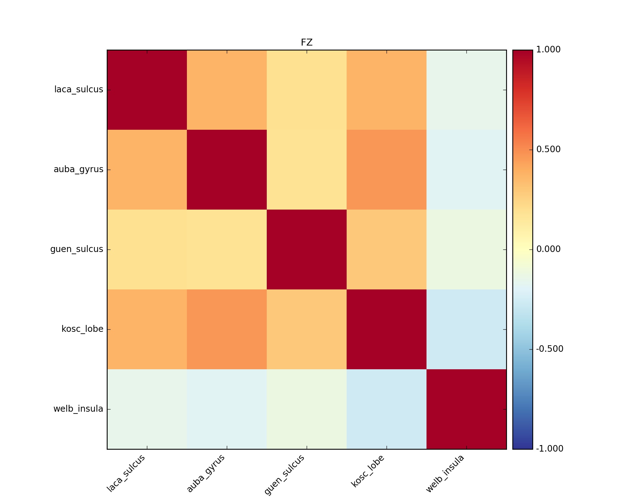
# make image of correlation matrix (Fisher-Z transform) of average ROI
# time series
fat_mat_sel.py \
-m ${ocorr}_000.netcc \
-P 'FZ' --A_plotmin=-1 --B_plotmax=1 \
--Tight_layout_on -x 10 --dpi=200 \
-M RdYlBu_r
cd ${ocorr}*INDIV
foreach ff ( `ls WB*nii.gz` )
set pp = `3dinfo -prefix_noext ${ff}`
@chauffeur_afni \
-ulay ../${vanat} \
-box_focus_slices ../${vanatss} \
-olay ${ff} \
-thr_olay 0.3 \
-cbar Reds_and_Blues_Inv \
-func_range 1 \
-opacity 6 \
-blowup 1 \
-save_ftype JPEG \
-prefix "${pp}" \
-pbar_saveim "${pp}_pbar.jpg" \
-montx 3 -monty 2 \
-set_xhairs OFF \
-label_mode 1 -label_size 3 \
-do_clean
end
cd ../
echo "++ DONE!"
exit 0
Notable outputs of |
do_03*.tcsh
|
|---|
NETCORR_000_INDIV/ |
sub-directory that holds the whole brain correlation maps of
each ROI’s average time series; there are also images of those
volumes stored there. |
NETCORR_000.netcc |
matrices of properties of the network of ROIs: Pearson
correlation coefficient (CC) and its Fisher-Z transform (FZ). |
NETCORR_000.netcc_FZ.jpg |
an image of the Fisher-Z transform (FZ) matrix |
NETCORR_000.netts |
text file containing the mean time series of each ROI |
NETCORR_000.roidat |
text file containing info of “how full” each ROI is–
basically, a way to check if masking or other processing steps
might have left null time series in any ROI mask. |
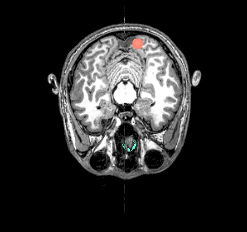
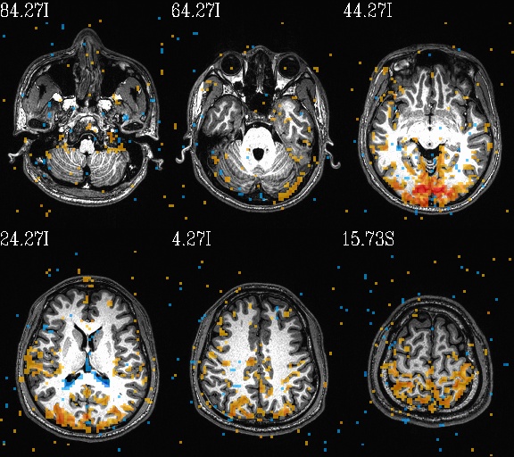
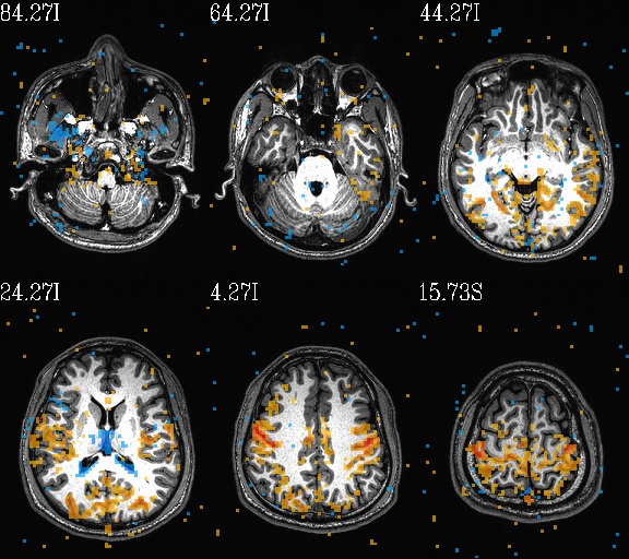
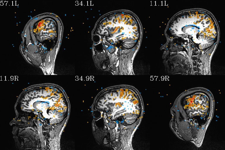
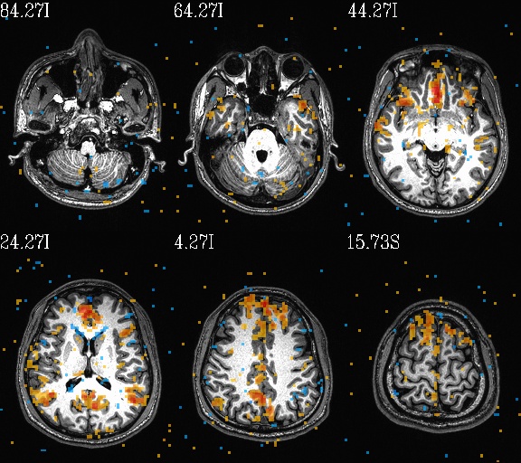
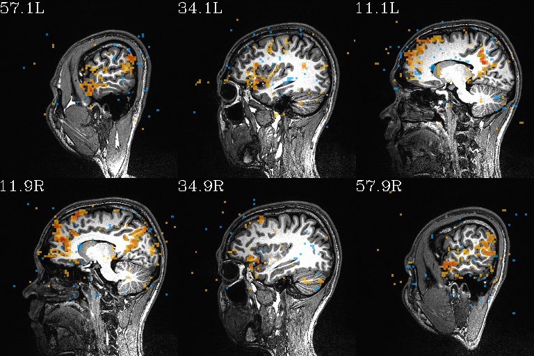
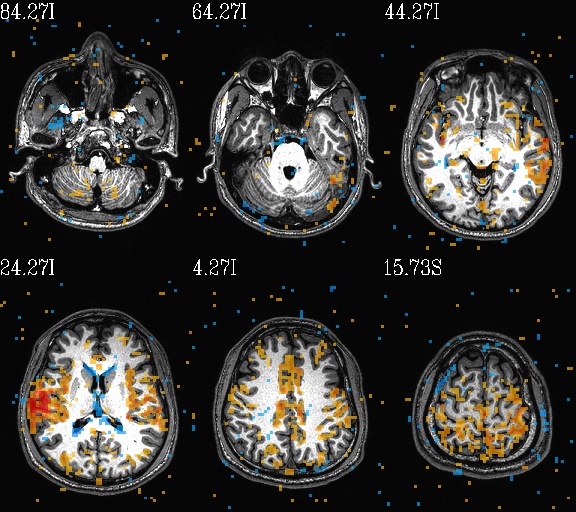
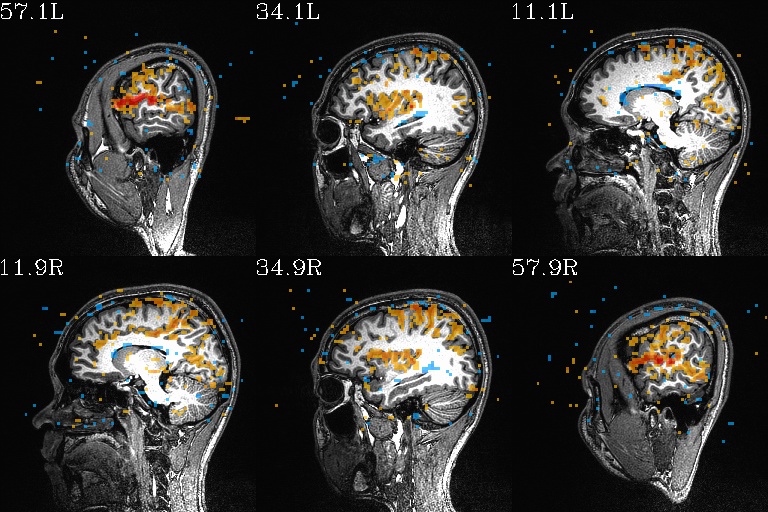
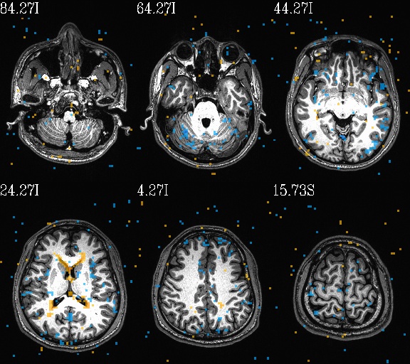
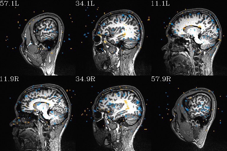
WB_Z_ROI*.jpg |
sets of images of the WB correlation maps of each ROI. Each
ROI has 3 images (axi, cor and sag viewplanes), and there is
also a “*_pbar.jpg” file of the colorbar used, and
“*_pbar.txt” file that records the colorbar min, max and
(optional) threshold value used. |
Some autoimages of do_03*.tcsh |
|
|---|
WB_Z_ROI_001.axi.jpg |
WB_Z_ROI_001.sag.jpg |
|
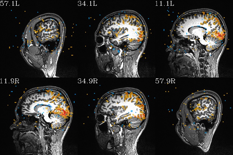
|
WB_Z_ROI_002.axi.jpg |
WB_Z_ROI_002.sag.jpg |
|
|
WB_Z_ROI_003.axi.jpg |
WB_Z_ROI_003.sag.jpg |
|
|
WB_Z_ROI_004.axi.jpg |
WB_Z_ROI_004.sag.jpg |
|
|
WB_Z_ROI_005.axi.jpg |
WB_Z_ROI_005.sag.jpg |
|
|
WB_Z_ROI_005_pbar.jpg |
WB_Z_ROI_005_pbar.txt |

|
-1 1 0.3
|
NETCORR_000_netcc_FZ.jpg |
|
|
|
