12.5.2. General fat_proc script properties
Specifying output location and prefix
Fortunately, the naming of outputs isn’t so complicated as that, but
one can essentially output with two names: a new subdirectory and a
prefix for filenames. For each fat_proc function, one can use
-prefix * to either put files of a given prefix into a preexisting
directory, or to both create a new subdirectory and put files of a
given prefix there. Thus, consider an example using -prefix
/somewhere/group/AAA/bbb:
if there is an existing directory “/somewhere/group/AAA/”, then this option would put files starting with “bbb” into it;
if there were just an empty, preexisting directory called “/somewhere/group/”, then this option would first create a new subdirectory “/somewhere/group/AAA/” and then populate it with files starting with “bbb”;
if there were just an empty directory called “/somewhere/”, then this option would lead to failure– it can only create a new output directory one layer deep.
Automatic QC imaging
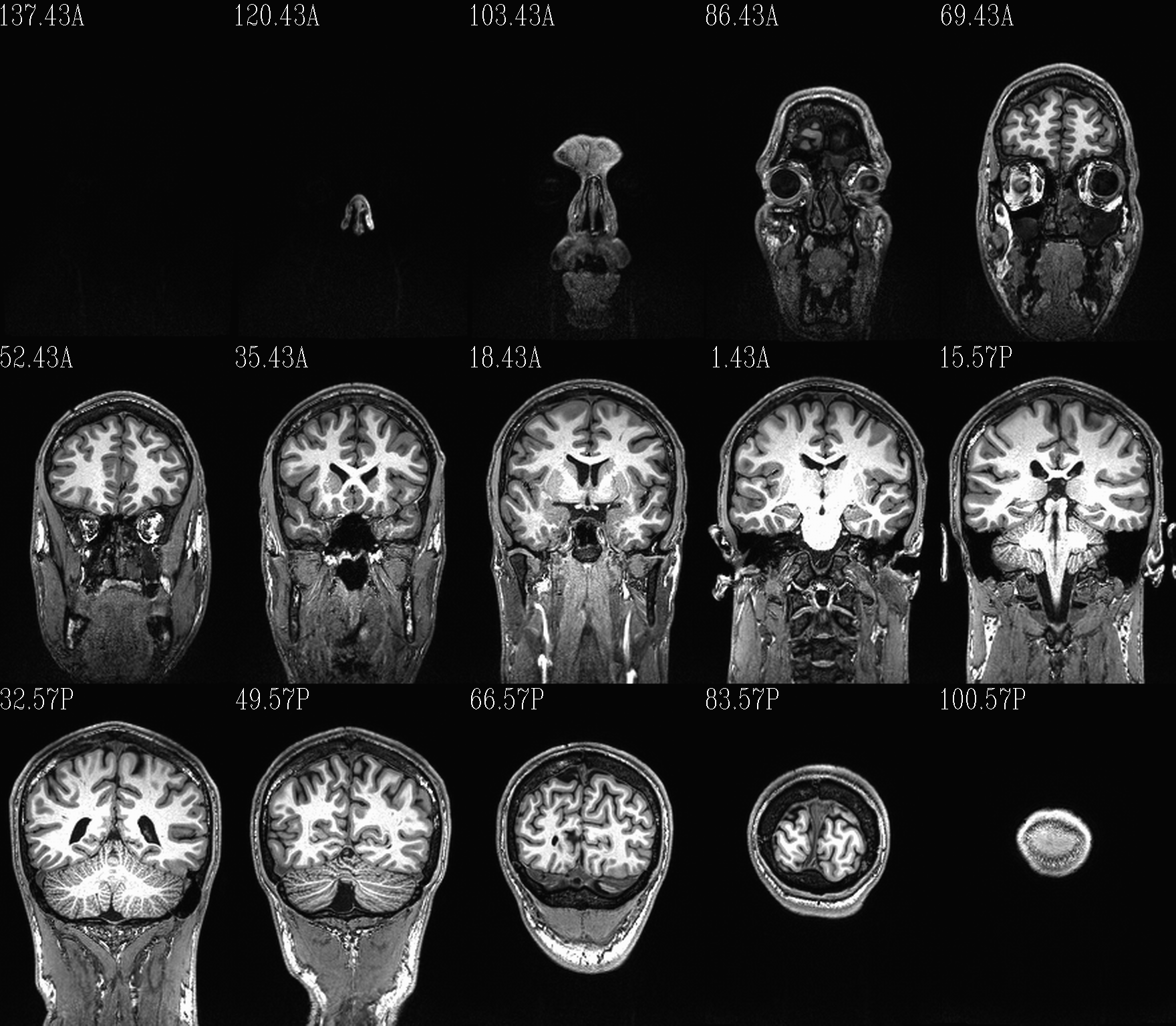
Most fat_proc functions automatically generate sets of montaged
images (PNG files by default). In each case the choice of image(s) is
mainly just due to what I thought might be useful or have found myself
creating often in order to evaluate a given step or the state of a
particular data set. These are done automatically by driving AFNI,
internally selecting overlays, thresholds, etc. that the user would
otherwise have to do by hand for each image, and saving everything in
an image file. By default, a set of axial, sagittal and coronal views
are made.
For 3D volumes, the montage size is typically 15 slices as evenly spaced as possible across each FOV dimension. These may show just an underlay, or underlays with either a translucent/masked overlay or an “edge-ified” image (esp. for judging alignment).
Definitions: * ulay: underlay data set; always grayscale here
olay: overlay data set; can be made using one of many colorscales, may also be translucent or outline edges
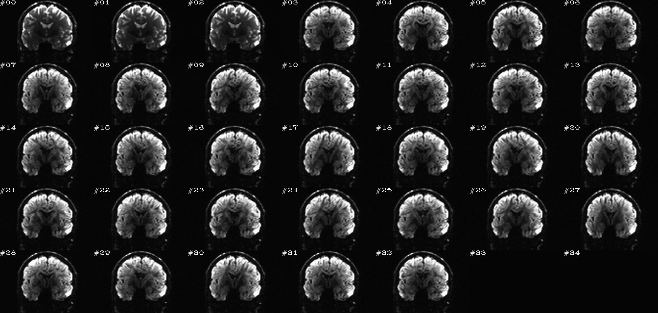
For 4D data, the montage typically shows a single slice across all time points (which, for DWI, might just represent different DW volumes). The N images are arranged in something close to a golden ratio array, padded at the end as necessary to have a solid grid of images. Additionally, a GIF or MPG movie may be created. Images may have a single scaling (grayscale: black=2% and white=98% brightness) across the whole volume (“onescl”) or separate scalings (again, 2-98%) for each volume (“sepscl”), each highlighting useful features for comparisons.
These images represent a benefit of batch processing: one can systematize the visual checks of processed data. That is, we can create very similar, comparable views across the group of data being processed, and then one can look through all these images quickly in succession to check for similarity or subtle patterns of difference. I find these sets of images very helpful for the process of understanding my data, checking the homogeneity of processing across a group, and seeing quickly any subjects that need to be reprocessed. These are also very useful sitting down with someone else (supervisor, student, colleague, etc.) and showing a lot of processed data quickly.
I typically process data on a Linux machine, and I use the eog
(Eye of Gnome) function to view lots of images in quick succession.
For example, say that I have data organized as a “group/” directory,
with subdirectories for each subject (“group/subj_001/”,
“group/subj_002/”, etc.) and some PNG files output in each
(img_QC_00.sag.png, img_QC_00.cor.png, img_QC_00.axi.png,
img_QC_01.sag.png, img_QC_01.cor.png, img_QC_01.axi.png, etc.). Then
I might be interested in looking at all the sagittal images from my
“*00*” QC test. I could load up the specified images from the
command line by typing with wildcards (”*”), for example:
eog group/subj_*/img*00*sag*png
I would then just need to hit the “right” and “left” arrow keys to go forward and backward through the list of images. NB: with eog, to see the full path for a file name, one can right click on any image and select “Properties” and see the path (and the field updates as one traverses images); additionally, one can set “View -> Side Pane” to see file information. I usually have “View -> Best Fit” toggled ON.
Note
It is possible to install eog on Mac OS. One might also
have another viewing program of choice– use whatever you
find easiest for viewing your data!
Temporary working directories
Most fat_proc functions perform several sub-steps, and therefore
they make use of temporary working directories. By default, these are
deleted or “cleaned up.” If you want to keep them, for example if
some step is failing and you want more information about why, you can
instruct them to not be deleted using the -no_clean switch.
Shell and scripting choices in these docs
The command line blocs in these tutorial docs will use tcsh
scripting notation from time to time, for example defining something
as a variable and then using that variable in a fat_proc function,
such as:
set dirname = "/data/DTI_EXAMPLE_DATA/data_proc/SUBJ_001/dwi_00"

fat_proc_something                  \
    -prefix $dirname/subj_314159    \
    ...
This is often done to simplify script reading, shortening lines by wrapping up long file paths into a single variable, or purely on whim.
Some people feel strongly about tcsh vs bash or other shells–
I am not smart enough to care deeply, fortunately or unfortunately.
Please feel free to translate any of these statements into whatever
shell or scripting language, such as Python, that you would wish.


