12.5.3. Pre-preproc, I: convert and niceify¶

Description ¶

Many of the following pre-preprocessing steps are convenience features for organizing, viewing, and assessing data, while at the same timing preparing to run major “pre”processing with several software functions. The present description page may look long, but much of that is to including snapshots of terminals and autoimages along the way.

The purposes of this set of scripts are:

to convert DICOMs to NIFTIs, putting (0, 0, 0) at the volume’s center of mass (useful for alignment, viewing, rotating) and giving all the same orientation (in particular, one with “x,y,z”-ordered coordinates, making the application of transformations simpler)
to allow the DWIs to be viewed, quality-checked and filtered according to the user’s judgment (e.g., remove dropout volumes or those with heavy motion distortion)
to filter volume, gradient and b-value files of a given data set simultaneously
to process dual phase encoded DWI data sets (i.e., when AP-PA data are present) in parallel, in order to maintain matched volumes/gradients
to axialize a reference anatomical (i.e., put it into “nice” alignment within a volume’s axes/orientation) for slice viewing, structure coloration, and group alignment
(if driven by necessity) to make an imitation T2w-like contrast reference volume if only a T1w is available; NB: ‘tis far better to have the real thing, probably, but one is not always available

You can skip any steps that aren’t applicable. I will assume that each acquired volume is currently a set of unpacked DICOMs sitting in its own directory. If a directory structure is set up well, it should be possible to loop through all subjects with the same few commands. (The filtering step, though, would likely require its own command per subject, as motion/distortion will occur in different volumes for different subjects.)

Note that each function listed below has its own helpfile, describing more details, defaults and available options. Here, default names and locations of things (such as output directories, prefixes, etc.) are often used in order to simplerify life.

Note

Having matched DWI data sets with opposite phase encoding (e.g., AP and PA) is useful for correcting EPI distortions. However, if you only have one, whether it is AP or PA doesn’t really matter for this pre-processing– I will refer to single phase encode data sets as ‘AP’ just for simplicity of description, but either encoding would get treated the same.

Example Setup ¶

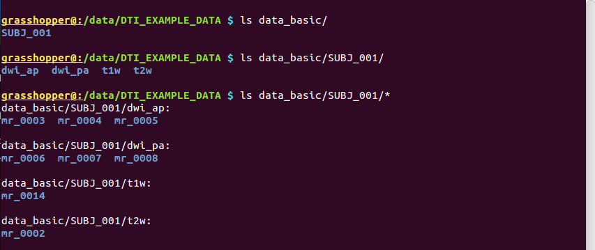
Consider starting with the following data set of a healthy, human adult in a diffusion-based study that is acquiring dual phase encoded DWIs. We make a group directory for a study (e.g., “DTI_GROUP_STUDY/”), with a tree for “raw,” unprocessed DICOMs (“data_basic/”) and one for processed volumes and files (“data_proc/”), with a subdirectory for each subject. Consider one subject’s directory (“SUBJ_001/”), which contains four sets of DICOM directories:

“dwi_ap/”: DWI set acquired with the phase encode direction anterior->posterior. There is one directory of DICOMs acquired with gradients for just DTI reconstruction (“mr_0003/”, with 3 volumes with b=0 volumes and 30 with b=1100 ${\rm s~mm^{-2}}$ ), and two others with higher b-valued shells for including with a more complicated reconstruction (“mr_0004/”, with 3 volumes with b=0 and 30 with b=2500 ${\rm s~mm^{-2}}$ ; “mr_0005/”, with 3 volumes b=0 and 30 with b=5000 ${\rm s~mm^{-2}}$ ). The spatial resolution is $2.5\times2.5\times2.5~{\rm mm}^3$ ; perhaps more standard/desirable would be 2~mm isotropic.
“dwi_pa/”: DWI set acquired with the same gradients as the AP one (with same respective shells stored in “mr_0006/” “mr_0007/” “mr_0008/”), though with the phase encode direction reversed, posterior->anterior.
“t2w/”: a T2w anatomical (with fat suppression– highly recommended if at all possible) with $1.25\times1.25\times1.70~{\rm mm}^3$ spatial resolution. This is still much higher resolution than the DWI data, which is great; perhaps isotropic resolution would be preferable.
“t1w/”: a T1w anatomical (standard MPRAGE) with $1\times1\times1 {\rm mm}^3$ spatial resolution.

Directory structure for example data set

Initial, basic subject directory layout: a branch of unprocessed data (“data_basic/”), containing one directory per subject (“SUBJ_001/”), containing one directory per type of dset (“dwi_ap/”, etc.), containing one or more directory of dicoms (“mr_00*/”).

Comments and notes ¶

In this primary example, we will reconstruct the set as follows. We will use both the AP and PA diffusion data in order to perform EPI distortion correction with DR_BUDDI, but we will employ just the set of DTI-like acquisitions (3 volumes with b=0 volumes and 30 with b=1100 ${\rm s~mm^{-2}}$ ). We will use the T2w volume as an anatomical reference within TORTOISE functions, and we will use the T1w volume for parcellation+segmentation in FreeSurfer.

Note

There will be a separate+parallel example description for the conversion and usage of all DWI sets. When I get time…

There will also be a separate description of processing as if there were no T2w volume, when I get even more time.

The help file of each function contains more options that are not listed in this “vanilla” processing description. It would behoove the reader to check those out.

Before processing, I have made a “data_proc/” directory that is parallel to the “data_basic/” one. The idea is that if I need to redo processing, I can move the entire tree and redo it. Additionally, as I loop through each subject directory in “data_basic/” (e.g., here, “SUBJ_001/”), I make a directory of the same name under “data_proc/” to hold all the processed data.

fat_proc_convert_dcm_dwis: Convert DWIs ¶

For each DWI set, go from DICOMs to having a NIFTI volume plus supplementary text files: a ‘*.bvec’ file has the unit normal gradients, and a ‘*.bval’ file has the diffusion weighting b-values.

The (x, y, z) = (0, 0, 0) coordinate of the data set is placed at the center of mass of the volume (and, when AP-PA sets are loaded, the sets could be given the same origin); having large distance among data sets create problems for rotating visualizations and for alignment processes. Volumes should all have the same orientation (“RPI” by default) and be anonymized (depends on things like filenames chosen; users should doublecheck anonymizing).

Proc: A paired set of N DWIs with opposite phase encode directions (in “data_basic/SUBJ_001/dwi_ap/” and “data_basic/SUBJ_001/dwi_pa/”):

# for I/O, "basic" (= DICOM) and "proc" (= NIFTI) directories
set path_B_ss = data_basic/SUBJ_001
set path_P_ss = data_proc/SUBJ_001

fat_proc_convert_dcm_dwis              \
    -indir  $path_B_ss/dwi_ap/mr_0003  \
    -prefix $path_P_ss/dwi_00/ap

fat_proc_convert_dcm_dwis              \
    -indir  $path_B_ss/dwi_pa/mr_0006  \
    -prefix $path_P_ss/dwi_00/pa

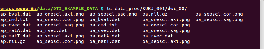
-> produces one new directory in ‘data_proc/SUBJ_001/’, called “dwi_00/”:

Directory structure for example data set

Output files made by fat_proc_convert_dcm_dwis commands for both the AP and PA data.

It contains the following outputs for the AP data (and analogous outputs for the PA sets):

Outputs of	`fat_proc_convert_dcm_dwis`
ap_cmd.txt	textfile, copy of the command that was run, and location
ap.nii.gz	volumetric NIFTI file, 4D (N=33 volumes)
ap_bval.dat	textfile, row file of N b-values
ap_rvec.dat	textfile, row file of (DW scaled) b-vectors ( $3\times N$ )
ap_cvec.dat	textfile, column file of (DW scaled) b-vectors ( $N\times 3$ )
ap_matA.dat	textfile, column file of (DW scaled) AFNI-style b-matrix ( $N\times 6$ )
ap_matT.dat	textfile, column file of (DW scaled) TORTOISE-style b-matrix ( $N\times 6$ )
*ap_onescl..png**	autoimages, one slice per DWI volume, with single scaling across all volumes
*ap_sepscl..png**	autoimages, one slice per DWI volume, with separate scalings for each volume

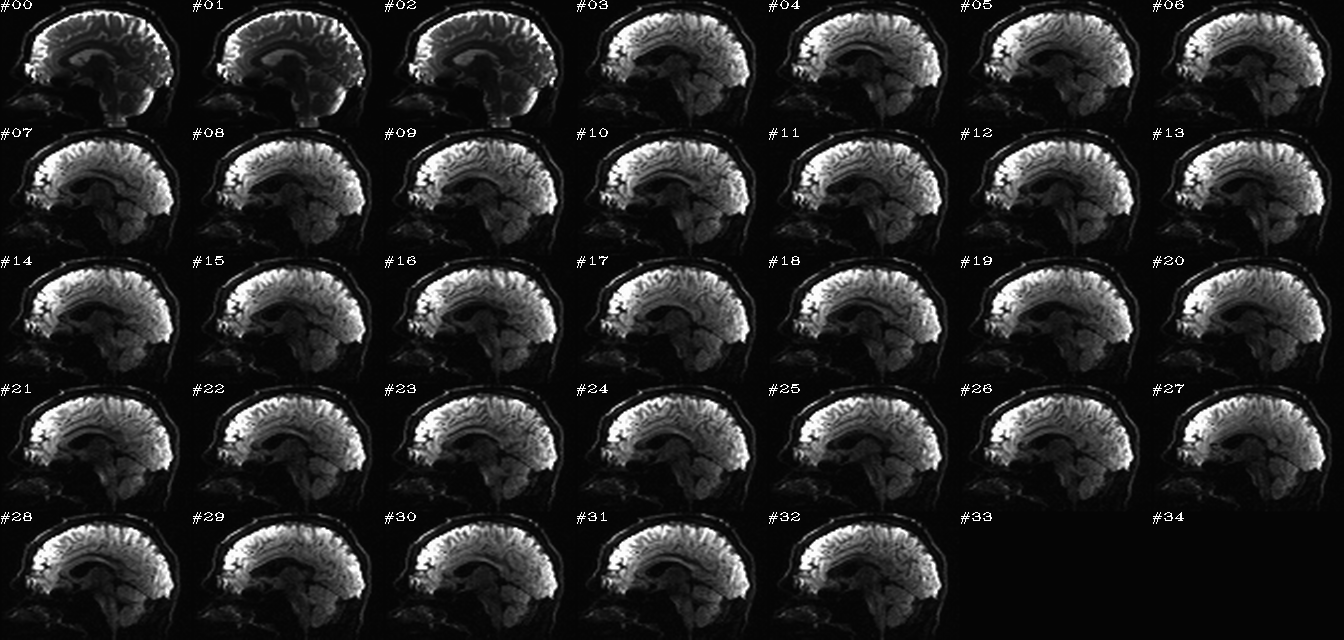
Autoimages of `fat_proc_convert_dcm_dwis`

PA volumes, separate scaling per volume, sagittal view. The integer numbers in the upper left hand corner (“#N”) of each panel are the volume number in the image. There are 33 volumes in this dset, with the final two blank panels (#33 and #34) merely appended for to display a full matrix.

AP volumes, separate scaling per volume, sagittal view. The image formatting is the same as above.

Note

Toggling between those sets of images highlights just why the AP-PA (or blip up-blip down) distortion correction for EPI inhomogeneity must be done. For example, you could open this on adjacent browser tabs and switch back and forth.

No gradient flipping has been performed (but it could be, if you wanted).

The AP and PA dsets match volume-for-volume. Interestingly, one can notice the difference in overall brain shape between the AP and PA dsets; for example, one can open each set in their own browser tabs and toggle back and forth.

fat_proc_convert_dcm_anat: Convert anatomical volume(s)¶

For each anatomical volume set (here, we have both a T1w and T2w volume), go from DICOMs to having a NIFTI volume.

As for DWIs above, the (x, y, z) = (0, 0, 0) coordinate of the data set is placed at the center of mass of the volume. Volumes should all have the same orientation (“RPI” by default) and be anonymized (depends on things like filenames chosen; users should doublecheck anonymizing).

Proc: Two separate anatomical volumes, a T1w and a T2w dset (in “data_basic/SUBJ_001/t1w/” and “data_basic/SUBJ_001/t2w/”):

# for I/O, same path variables as above in the DWI case
set path_B_ss = data_basic/SUBJ_001
set path_P_ss = data_proc/SUBJ_001

fat_proc_convert_dcm_anat              \
    -indir  $path_B_ss/t1w/mr_0014     \
    -prefix $path_P_ss/anat_00/t1w

fat_proc_convert_dcm_anat              \
    -indir  $path_B_ss/t2w/mr_0002     \
    -prefix $path_P_ss/anat_00/t2w

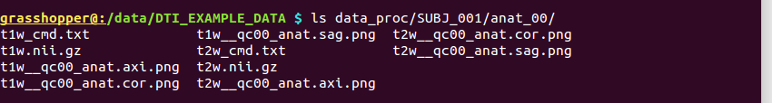
-> produces one new directory in ‘data_proc/SUBJ_001/’, called “anat_00/”:

Directory structure for example data set

Output files made by fat_proc_convert_dcm_anat commands for both the T1w and T2w data.

It contains the following outputs for the T1w data (and analogous outputs for the T2w sets):

Outputs of	`fat_proc_convert_dcm_anat`
t1w_cmd.txt	textfile, copy of the command that was run, and location
t1w.nii.gz	volumetric NIFTI file, 3D (single brick volume)
*t1w__qc00_anat..png**	autoimages, multiple slices per DWI volume, with single scaling across the volume

Autoimages of `fat_proc_convert_dcm_anat`

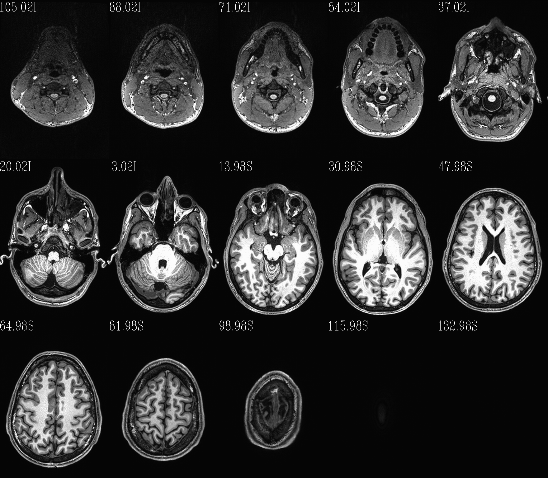
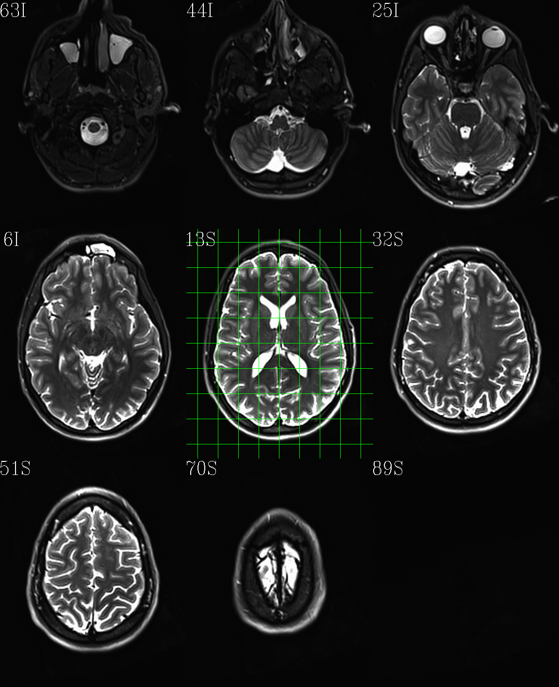
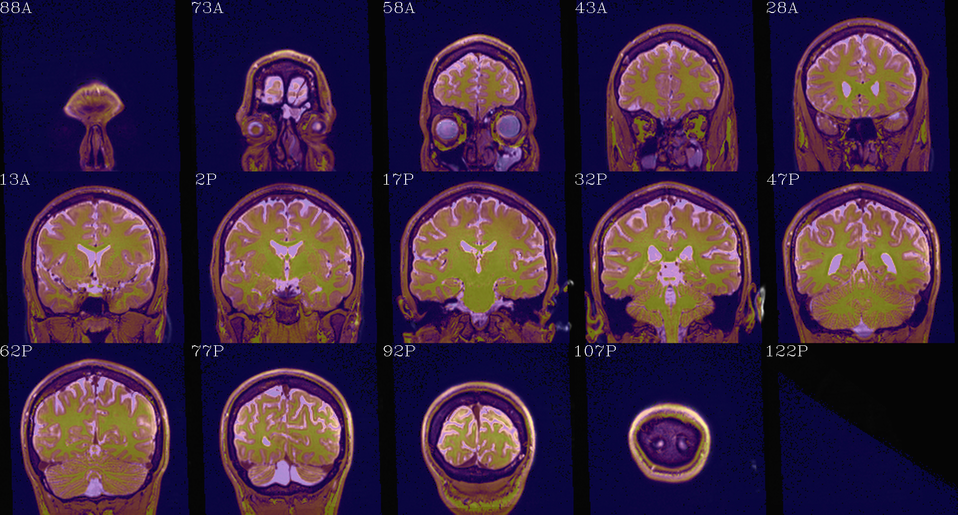
Slices of the T1w volume, single scaling for the volume, axial view. The float numbers in the upper left hand corner (“#XI” and “#XS”) of each panel are the physical space coordinate for that slice (in RAI-DICOM notation, which is default in the AFNI GUI viewer).

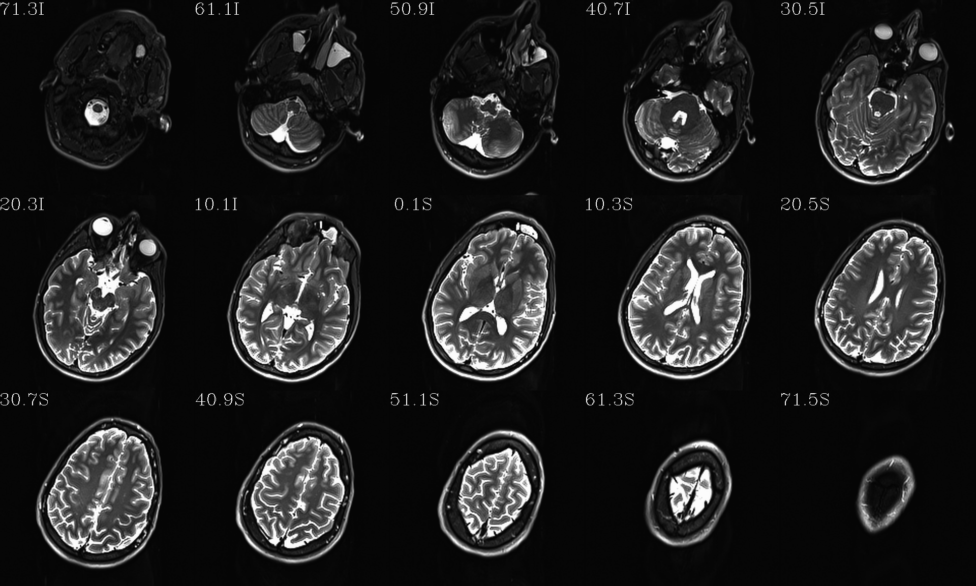
T2w volumes, single scaling per volume, axial view. The image formatting is the same as above.

Note

Notice that here the T2w volume is really quite oblique to the acquired field of view (FOV). When using this as a reference volume in TORTOISE, the DWI volumes would also end up with major axes unaligned to those of the dset FOV; this would be highly non-ideal for things like RGB coloration and systematic viewing/comparisons. This is dealt with in the next step (“axialization”).

fat_proc_axialize_anat: Axialize the anatomical ¶

There are many reasons why it would be useful to have subject volumes well-aligned (i.e., major brain axes aligned with the volume’s FOV, so that slices planes are in “standard” viewing orientation):

for group alignment, all volumes start “nearer” to each other
views across the group are more similar and therefore easier to compare and/or spot differences and similarities
since the T2w volume will be useful for DWI reference alignment in TORTOISE, then alignment leads to RGB coloration of structures in DWI being both uniform across group and standardly interpretable (e.g., transcallosal regions are red; cingular fibers are green; cortico-spinal tracts are mainly blue).

If a subject’s head is strongly tilted in the volumetric FOV, then the display of slices might be awkward, anatomical definition might be tricky, tract/structure coloration could be non-standard, and later alignments might be made more difficult.

The present “axialization” process is akin to an automated form of “AC-PC alignment” that is sometimes performed (for example, using MIPAV)– but, importantly, it is not the same thing. This program “rights the ship” by calculating an affine alignment to a reference volume of the user’s choice (e.g., a standard space Talairach volume), but only applying the rotation/translation part, so that the subject’s brain doesn’t warp/change shape (and brightness values are not altered, except by minor smoothing due to rotation).

Axialization can be applied to either a T2w or T1w volume. The “mode” of running must be specified, basically as whether the volume in question has either contrast similar to a human adult’s T2w volume (-mode_t2w) or T1w volume (-mode_t1w). The mode selection mainly specifies some processing options internally. Note that for newborn infant dsets, one might invert the mode flag (i.e., use -mode_t1w for an infant T2w volume), because the contrasts at young ages are inverted. Sigh, I know, that’s not ideal, but that’s life at present.

Proc: This takes the NIFTI T2w dset (in “data_proc/SUBJ_001/anat_00/”) and axializes it with respect to the reference dset (here, from the MNI 2009 templates, which was manually AC-PC aligned and regridded to have an even number of slices in all FOV planes as described here and downloadable from here on the AFNI website), with some extra weighting for the subcortical regions (via -extra_al_wtmask *); and the output volume will match the grid of the input volume (-out_match_ref):

# I/O path, same as above; just need the "proc" dirs now
set path_P_ss = data_proc/SUBJ_001

# reference anatomical volumes to which we axialize
set here       = $PWD
set ref_t2w    = $here/mni_icbm152_t2_relx_tal_nlin_sym_09a_ACPCE.nii.gz
set ref_t2w_wt = $here/mni_icbm152_t2_relx_tal_nlin_sym_09a_ACPCE_wtell.nii.gz

fat_proc_axialize_anat                       \
    -inset  $path_P_ss/anat_00/t2w.nii.gz    \
    -prefix $path_P_ss/anat_01/t2w           \
    -mode_t2w                                \
    -refset          $ref_t2w                \
    -extra_al_wtmask $ref_t2w_wt             \
    -out_match_ref

-> produces one new directory in ‘data_proc/SUBJ_001/’, called “anat_01/”:

Directory structure for example data set

Output files made by fat_proc_axialize_anat commands for the T2w data set.

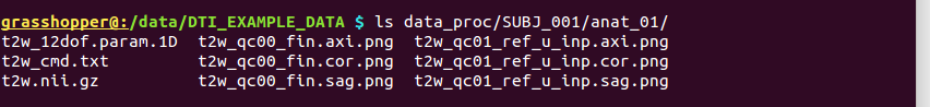
It contains the following outputs for the T2w data:

Outputs of	`fat_proc_axialize_anat`
t2w_cmd.txt	textfile, copy of the command that was run, and location
t2w_12dof.param.1D	textfile, the 12 DOF linear affine transformation matrix produced by `3dAllineate` during the processing; this is the applied transformation, so only the solid body (translation+rotation) elements of the matrix can be nonzero.
t2w.nii.gz	volumetric NIFTI file, 3D (single brick volume), now axialized (hopefully)
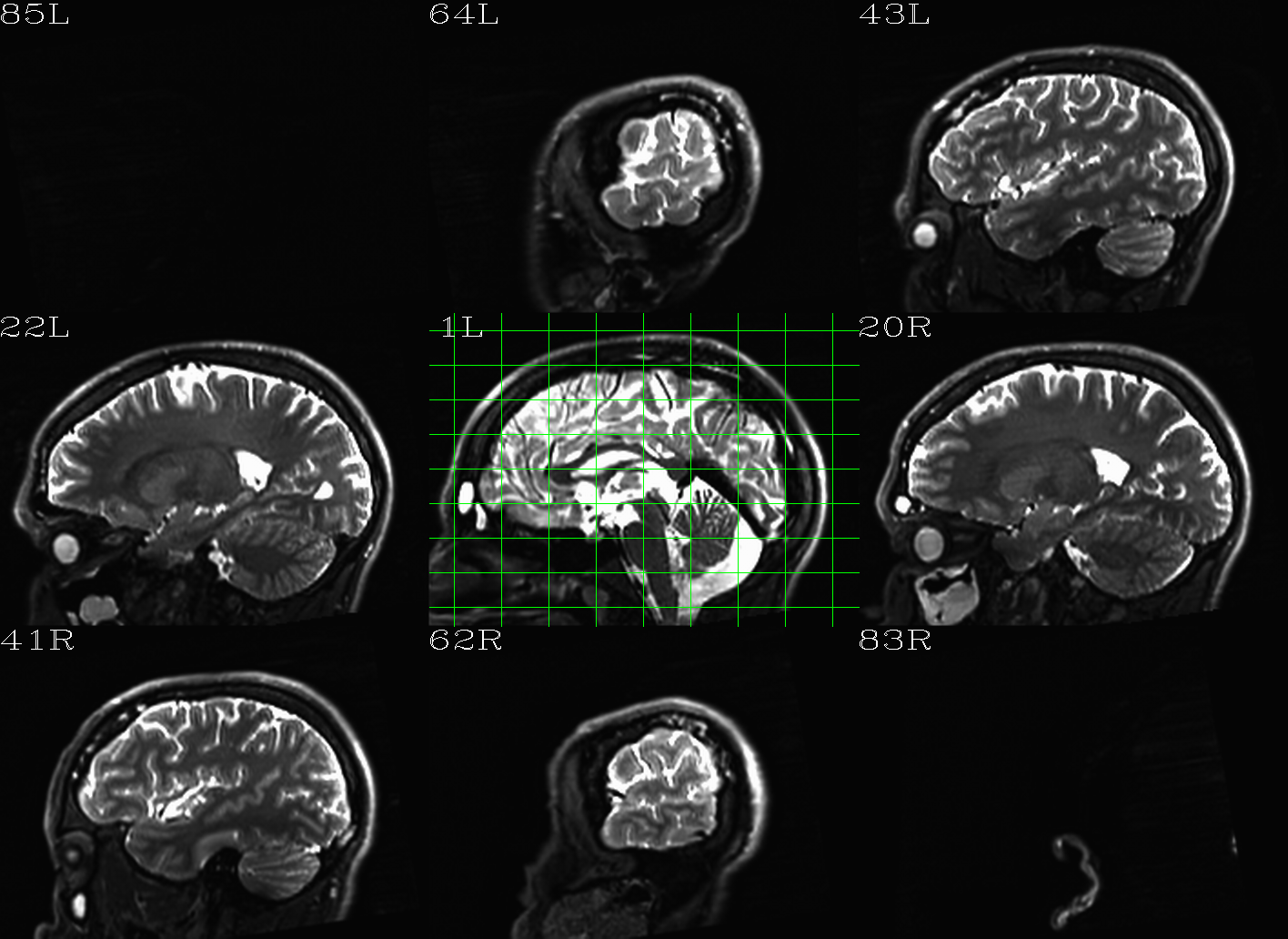
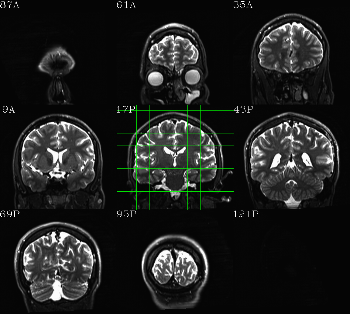
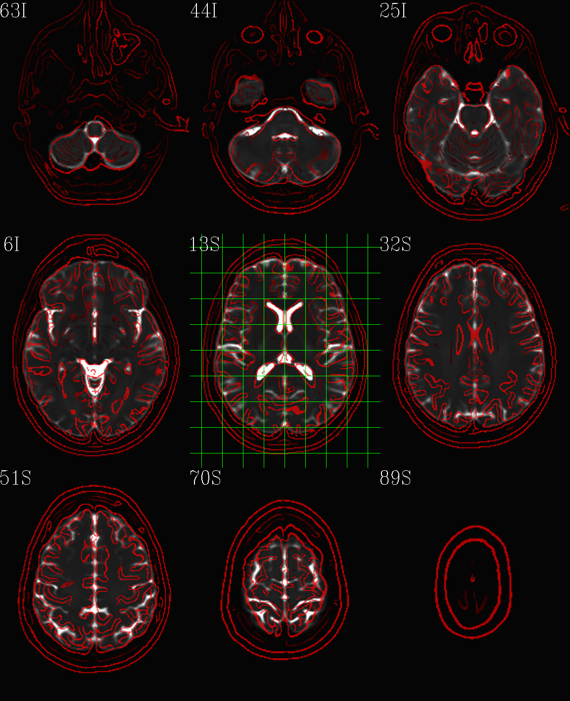
*t2w_qc00_fin..png**	autoimages, multiple slices per 3D volume, with single scaling across the volume, showing the final axialized volume; grid slice lines are also shown in the central volume, for visual reference of major plane lines.
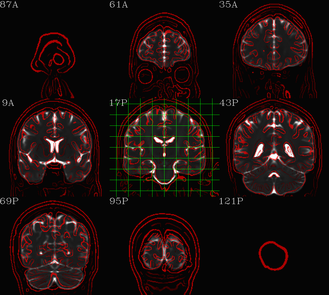
*t2w_qc01_ref_u_inp..png**	autoimages, multiple slices per 3D volume; the image is in the space of the `-refset ` with single scaling across the ulay volume (the reference dset); the olay dset is an edge-ified version of how the `-inset ` volume was aligned to it, for QC and possible trouble-shooting purposes.

Autoimages of `fat_proc_axialize_anat`
t2w_qc00_fin.*.png	t2w_qc01_ref_u_inp.*.png



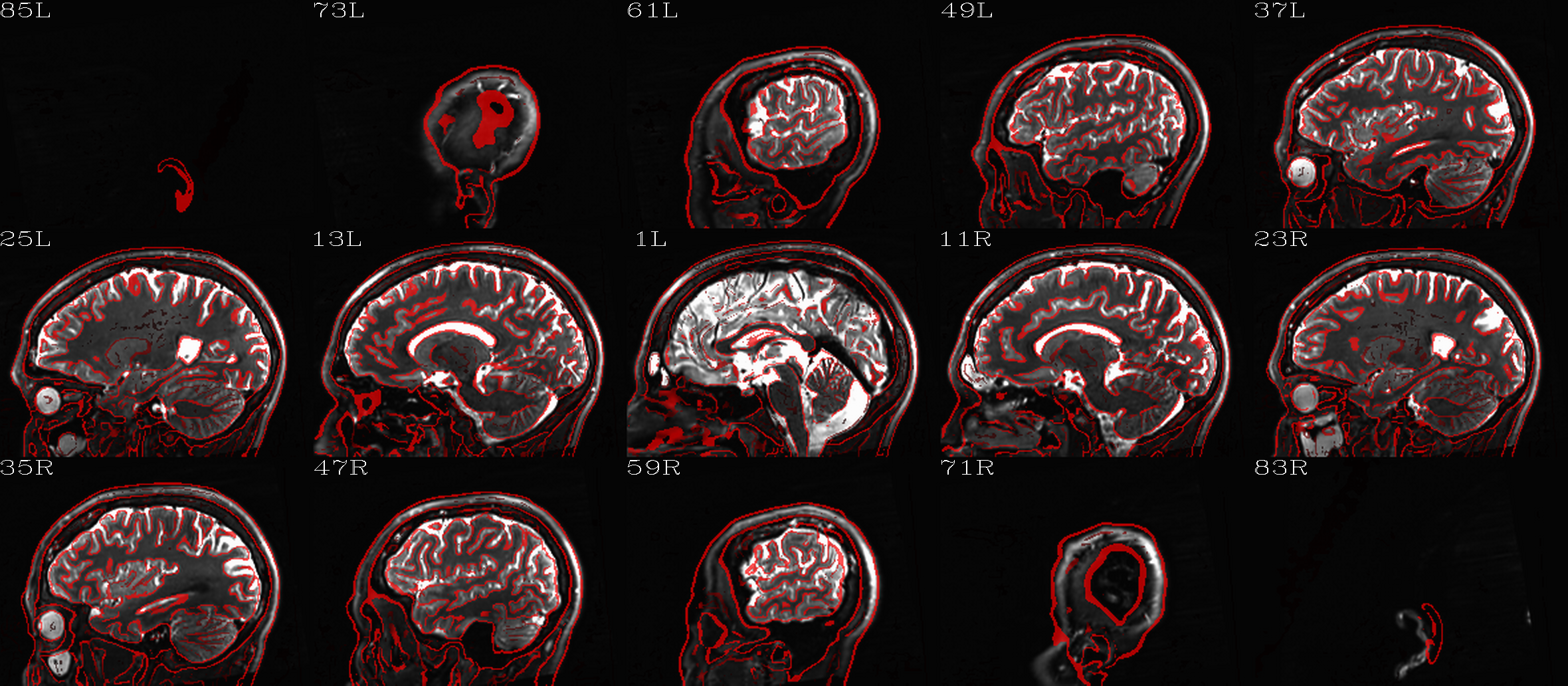
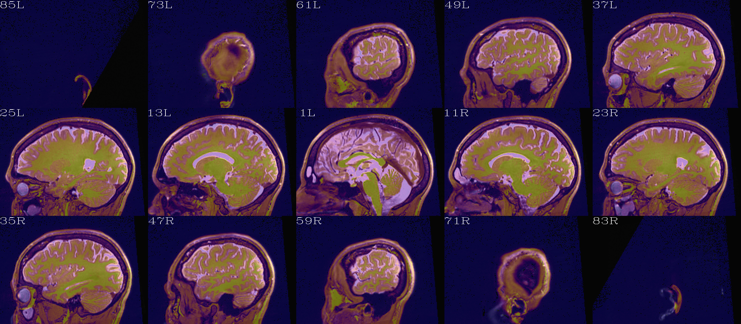
Images of the final volume, for checking the alignment of brain structures with major FOV axes.	Intermediate volume images, for checking the relative goodness of alignment fit of the anatomical (edge-ified olay) with the refset volume (ulay).

TIPS:

For any anatomical, it might useful to resample the volume to isotropic, fairly high resolution both for viewing and later registration purposes. This could be done by outputting on the refset’s grid, or also by specifying an isotropic resolution, such as to isotropic $1 {\rm mm}^{3}$ using:
```
-extra_al_opts "-newgrid 1.0"
```
Something similar (perhaps using a different resolution) might be useful in most cases with this function.
When things go wrong with alignment, and the dsets don’t appear to overlap much at all, it could be that they started too far apart in the first place; using -pre_center_mass might help provide an initial alignment, esp. if a either the inset or refset is not well-centered– i.e., center of mass near (0,0,0)– in the first place.
Sometimes, anatomical volumes will have lots of non-brain material in the FOV, such as neck and sub-brain volumes. When that is the case, the center of mass of the FOV might be moved “down” with respect to a reference volume. In such a case, it might be useful to pre-remove some number N of axial slices from the inferior part of the FOV, using -remove_inf_sli N; in conjunction with -pre_center_mass, this might provide a better starting point for alignment (NB: this “removal” is only for alignment purposes; the final dset will not have any slices removed from this).

fat_proc_align_anat_pair: Align T1w -> T2w ¶

At this point, it might be useful to align the T1w anatomical to the newly axialized T2w volume. Then, the T1w itself should be axialized. NB: by default, this alignment is just a “solid body” (rotation + translation) transformation, so there is no change in shape of the T1w volume (besides the minimal amounts of smoothing involved with regridding); if desired, one can provide an option to fat_proc_align_anat_pair to allow for any set of the full linear affine parameters available in 3dAllineate.

Additionally, if one is aiming to run FreeSurfer’s recon-all on the T1w, this step can be useful for preparing the volume for that. In particular, at present (FreeSurfer versions up to 6.0) the function seems to tacitly require having:

isotropic voxels:
- 1 mm edges, by default.
- for higher resolution (sub-millimeter) data, the FreeSurfer website states:
  
  “The method works well for voxel sizes 0.75 mm3. It should work with voxel between 1mm3 and 0.75mm3. Inputs with 0.5 mm3 voxels or below will have a brainmask failure…”
  
  ... and one should use the -hires flag in recon-all for such data.
even numbers of slices in all directions of the dset FOV; not having this will affect results negatively.

These properties can be conveyed to the T1w dset at this stage.

Note

This step is quite optional. However, if one doesn’t align the volumes now, one should still take care that the T1w volume does have the above properties before FreeSurfering with recon-all.

Proc: Align the T1w (in “data_proc/SUBJ_001/anat_00/”) and align it to the axialized T2w volume (in “data_proc/SUBJ_001/anat_01/”); the T2w volume here has both isotropic voxels with 1 mm edges and even numbers of slices in all directions, so we make the T1w volume output be on the same grid, so it has these properties, as well (there are other options for controlling these things, as well):

# for I/O, same path variable as above
set path_P_ss = data_proc/SUBJ_001

fat_proc_align_anat_pair                     \
    -in_t1w    $path_P_ss/anat_00/t1w.nii.gz \
    -in_t2w    $path_P_ss/anat_01/t2w.nii.gz \
    -prefix    $path_P_ss/anat_01/t1w        \
    -out_t2w_grid

-> produces new data in the existing directory in ‘data_proc/SUBJ_001/anat_01’, because the new T1w volume is essentially in the same space as the reference T2w volume now.

Directory structure for example data set

Output files made by fat_proc_align_anat_pair commands for the T1w data set (t1w), as well as the earlier-made T2w reference volume (t2w).

It contains the following outputs for the T2w data:

Outputs of	`fat_proc_axialize_anat`
t1w_cmd.txt	textfile, copy of the command that was run, and location
t1w_map_anat.aff12.1D	textfile, the 12 DOF linear affine transformation matrix produced by `3dAllineate` during the processing.
t1w.nii.gz	volumetric NIFTI file, 3D (single brick volume), now aligned to the T2w volume.
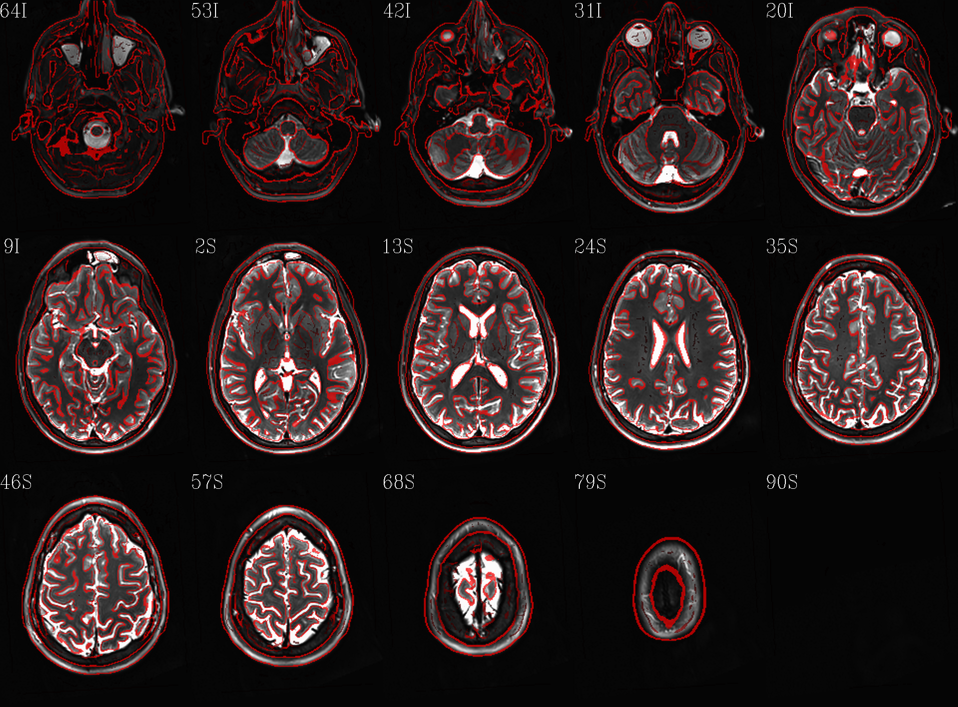
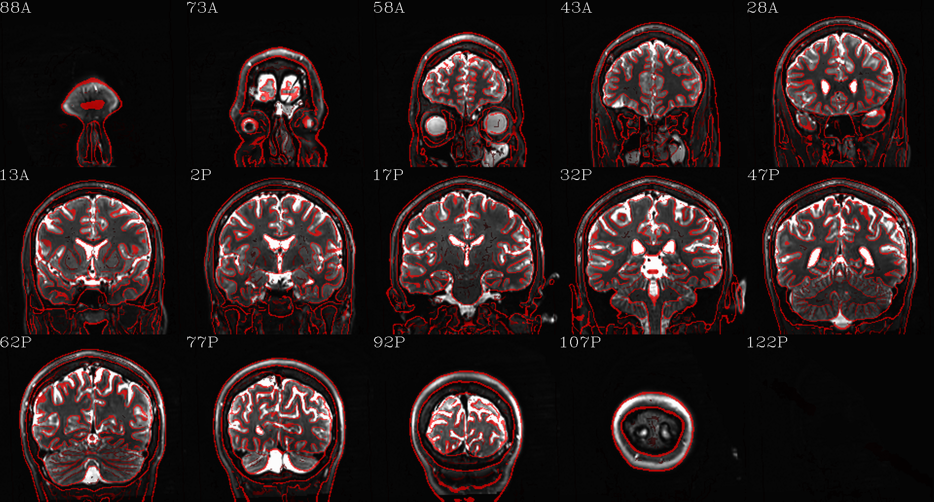
*t1w__qc00_t2w_u_et1w..png**	autoimages, multiple slices per 3D volume, with single scaling across the volume, showing the T2w reference as the ulay, and an edge-ified version of the T1w volume as the olay, to just the quality of fitting by sulcal features, tissue boundaries, etc.
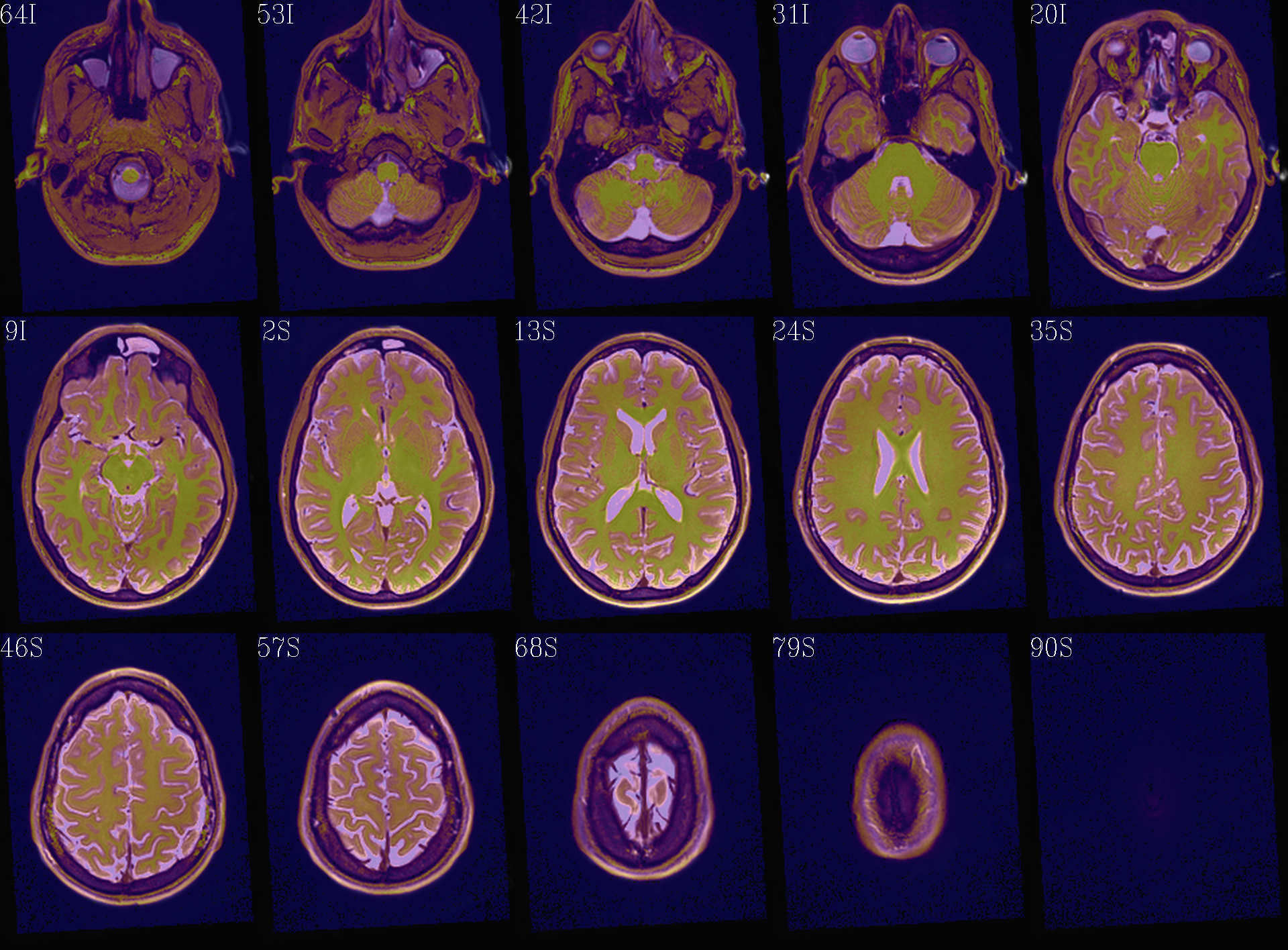
*t1w__qc01_t2w_u_t1w..png**	autoimages, multiple slices per 3D volume; the T2w reference as the ulay, with a translucent version of the T1w volume as the olay.

Autoimages of `fat_proc_align_anat_pair`
t1w__qc00_t2w_u_et1w.*.png	t1w__qc01_t2w_u_t1w.*.png



T2w reference as ulay, with edge-ified final T1w volume as olay, for checking the alignment of brain structures.	T2w reference as ulay, with translucent final T1w volume as olay, for checking the alignment of brain structures.

12.5.3. Pre-preproc, I: convert and niceify¶

Description ¶

Example Setup ¶

Comments and notes ¶

fat_proc_convert_dcm_dwis: Convert DWIs ¶

fat_proc_convert_dcm_anat: Convert anatomical volume(s)¶

fat_proc_axialize_anat: Axialize the anatomical ¶

fat_proc_align_anat_pair: Align T1w -> T2w ¶

Table of Contents

This Page

Quick search