12.5.1. Background and additional software
Overview
This page provides a preliminary description of using AFNI+FATCAT tools to develop a flexible pipeline for the processing and analysis of diffusion-based images. We describe the available tools and give example commands for real sets of data that have been acquired in various ways.
Importantly, these functions combine and are designed to integrate
smoothly with existing processing tools. This includes TORTOISE for processing diffusion weighted
(DW) MRI data. It also uses dcm2niix from mricron (though,
conveniently, this is now distributed within AFNI itself, as
dcm2niix_afni– thanks, C Rorden!) for converting DICOM files to
NIFTI format. Additionally, we describe incorporating FreeSurfer into the processing, as one
way of making meaningful GM targets from the subject’s own data.
Note
TORTOISE has changed quite a lot lately (early-mid 2017), and we now just describe using tools in TORTOISE v3.* (or potentially later, as time rolls on inexorably). This is version is command line processable, and has several new features relative to v2.* and earlier.
For now, we do still provide the earlier PDF for how we run straightforward processing in TORTOISE v2.5.2, for those in the midst of processing older data still. However, we strongly recommend using the more recent versions described.
While there is no single way to break up levels of a processing pipeline, the major stages can be described as follows:
Pre-preprocessing. First, we discuss converting DW and anatomical data sets from DICOM format, organizing them, preparing the anatomical as a reference volume (and also for segmentation), visually checking the DWIs and removing bad volumes/gradients.
Preprocessing. We then provide a brief set of steps for using the TORTOISE GUI to process your DWI data. Note, we don’t maintain the TORTOISE tools, we just use them a lot; please consult with the real TORTOISE gurus for processing, and take everything here with a grain of salt. We describe some default usages, but special cases (infant, pediatric, non-typical brain structure, non-human brains, etc.) should really involve the TORTOISE gurus. We also describe running FreeSurfer and converting volumes to AFNI/SUMA format.
Post-preprocessing. We then show simple steps for tensor fitting and parameter estimation, as well as basic whole brain tracking for quality control. We even discuss some further processing, for example integrating with FreeSurfer (and maybe eventually FMRI data, or other things…), but the branching points for analysis become pretty numerous pretty quickly.
It is pretty difficult to come up with one unwavering pipeline for this preprocessing, particularly as people have very different data. For example, were the DWIs acquired using a single phase encode direction, or a pair of oppositely phase encoded (AP-PA, blip-up/blip-down data)? Scans of squirmy kids, or meditating adults? Is there a T2w anatomical, or only a T1w volume? Therefore, we describe a possible sequence of tools, but mention that not all would be necessary (or even appropriate, in some cases) in every single pipeline. The user will be required to do some decision making.
A schematic pipeline for some of the main |
|---|
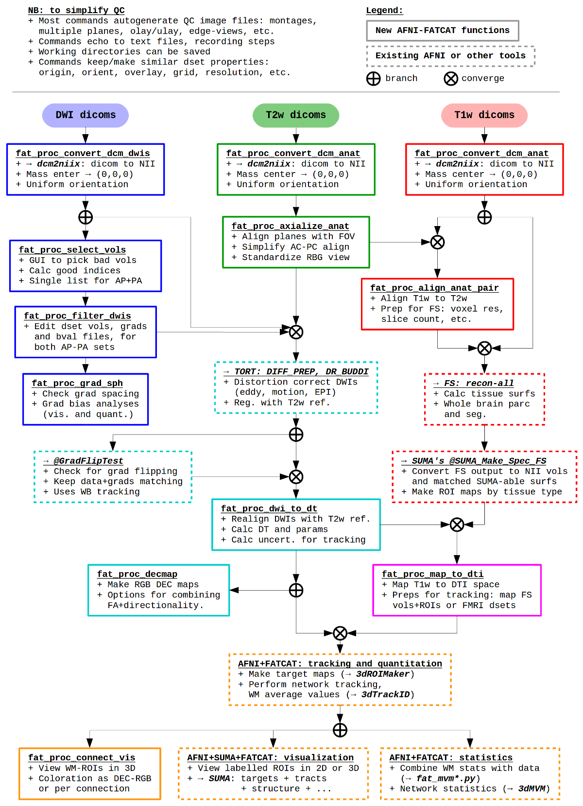
|
These scripts are examples, not dogma– they are a way to go about
DWI processing with AFNI, FATCAT and TORTOISE (as well as FreeSurfer
and dcm2niix). They are bound to change (improve?) over
time. Additional options can happily be added if they simplify your
life and don’t overly complicate mine. And please let me know if you
have any problems, via posting on the Message Board or emailing.
Much of this work was started at the University of Cape Town, SA– thanks Jia Fan, Marcin Jankiewicz and Ernesta Meintjes for facilitating and providing useful feedback with many of these scripts. Additionally, thanks Bharath Holla at NIMHANS in Bangalore, India, who also ran beta versions and gave very helpful suggestions.
TORTOISE and DWIs
Diffusion weighted MRI data can be greatly affected by a large number of artifacts. The most (in)famous are probably subject motion, eddy current distortion and EPI distortion (B0 inhomogeneity). Trickiness in dealing with their effects is compounded by the fact that their distortions themselves are compounded and can’t really be separated. Trying to manage them is serious business, and a combination of thoughtful study design and careful data acquisition is as important (if not more so) than any computational processing afterwards.
TORTOISE (Pierpaoli et al., 2010) is a very effective retrospective processing tool for acquired DWIs, and it is publicly available from the NIH. As noted on their webpage, there are two main tools in TORTOISE for corrective preprocessing of diffusion data:
DIFFPREP- software for image resampling, motion, eddy current distortion, and some EPI distortion correction using a structural image as target, and for re-orientation of data to a common space.
DR_BUDDI- software for EPI distortion correction using pairs of diffusion data sets acquired with opposite phase encoding (blip-up blip-down acquisitions), also using a structural image as a target.
By default, these functions use an anatomical reference for distortion
correction/unwarping, and it is strongly recommended to have one when
using TORTOISE. The anatomical data set should match the contrast of a
subject’s b=0 DWI volume, which generally means having a
T2-weighted (T2w) volume; the application of a T1w volume as a
reference if a T2w one is not available is discussed below. Finally,
we note that TORTOISE includes the DIFF_CALC module for tensor
fitting, visualization and other features, but here it is only used
for exporting DIFFPREP or DR_BUDDI results.
As also noted on their webpage, it is not a speedy program– though it
has gotten much faster in v3.* (having migrated from IDL to
C++). Speed of processing depends a lot on the data, with higher
spatial resolution, larger numbers of volumes/gradients and greater
upsampling adding to time. It might take around an hour to
DIFFPREP a standard research data set (~30 grads, 2 mm isotropic
data), and probably a couple hours then for DR_BUDDI
Many thanks to Okan Irfanoglu, Amritha Nayak, Carlo Pierpaoli and the rest of the TORTOISE crew for constructive comments, suggestions and contributions to these notes and scripts.
DICOMs and dcm2niix(_afni)
DICOM conversion requires reading the data header, parsing it for desired information (i.e., how many volumes, what order, voxel dimensions, etc.), and putting it all into a usable format such as NIFTI plus supplementary text files. Many things in the DICOM world aren’t standardized, vendors do things independently (and change their own inner workings from time to time), and tailored sequences might contain additional wrinkles. Basically, it’s a hard task.
There’s a fair number of DICOM converters out there and even some “in
here” in AFNI (e.g., to3d, Dimon). I use dcm2niix_afni
for conversion because: it is free (and now even distributed as part
of AFNI!); I have used it for a long time; it requires minimal user
input; and I’ve generally found it to be reliable– that is, most
converted volumes (appear to) have correctly translated data and
header information. However, there are no guarantees in life, and the
user will be expected to look over her/his own data for sanity
checking everything.
Previously, the TORTOISE folks have typically recommended reading in DICOM files to TORTOISE directly. This is because they have managed their own set of DICOM-readers and felt that they stay up-to-date with vendor changes and it is therefore the most stable way to go. As of TOROISE v3.1, however, I believe they also now implement dcm2niix for most cases, so this difference is also much reduced. The choice of whether to convert or not before TORTOISEing is still yours, though, dear user. Note that for special kinds of acquisitions (e.g., those made with: oblique acquisitions, home-cooked sequences, some scanner vendors, image gradients wrapped in with the diffusion gradients, etc.), extra care must be taken and talking with the TORTOISE folks directly is recommended. I do like to convert DICOMS to NIFTI so that I can view the data and kick out bad volumes pre-TORTOISEing, and I haven’t had the misfortune to have major formatting trouble whilst doing so (he writes asking The Universe for trouble…).
Note
When converting DICOMs, it seems like one has to be extra vigilant when converting data acquired on Philips scanners. This is not to pick on anybody, but there have been many times when reading header information properly has been challenging. Looking at data, and testing it to make sure it has the properties you expect, is always a Good Thing.
We try to maintain fairly recent copies of dcm2niix in AFNI. Any
deep questions on converting DICOMs with this tool should be directed
to C. Rorden et al., though we are happy to learn of
updates/fixes/etc.
Supplementary/reference data sets
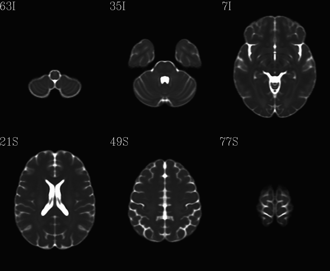
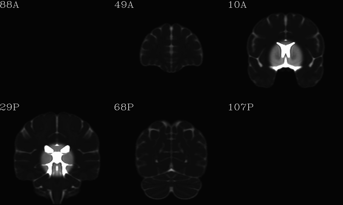
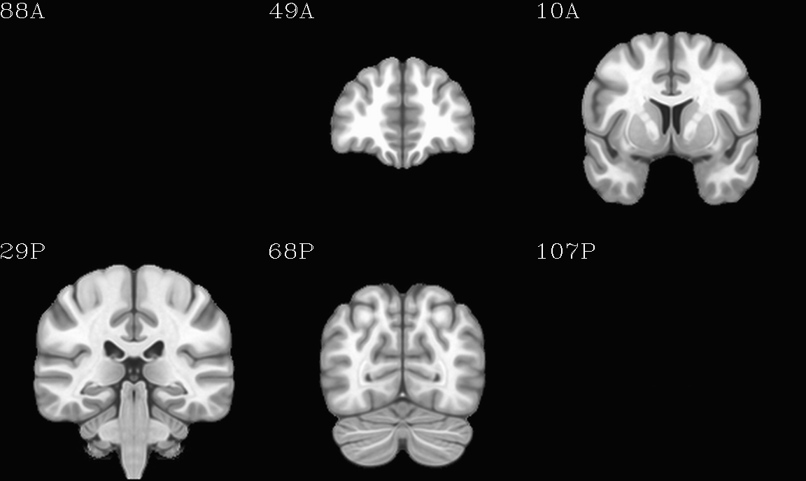
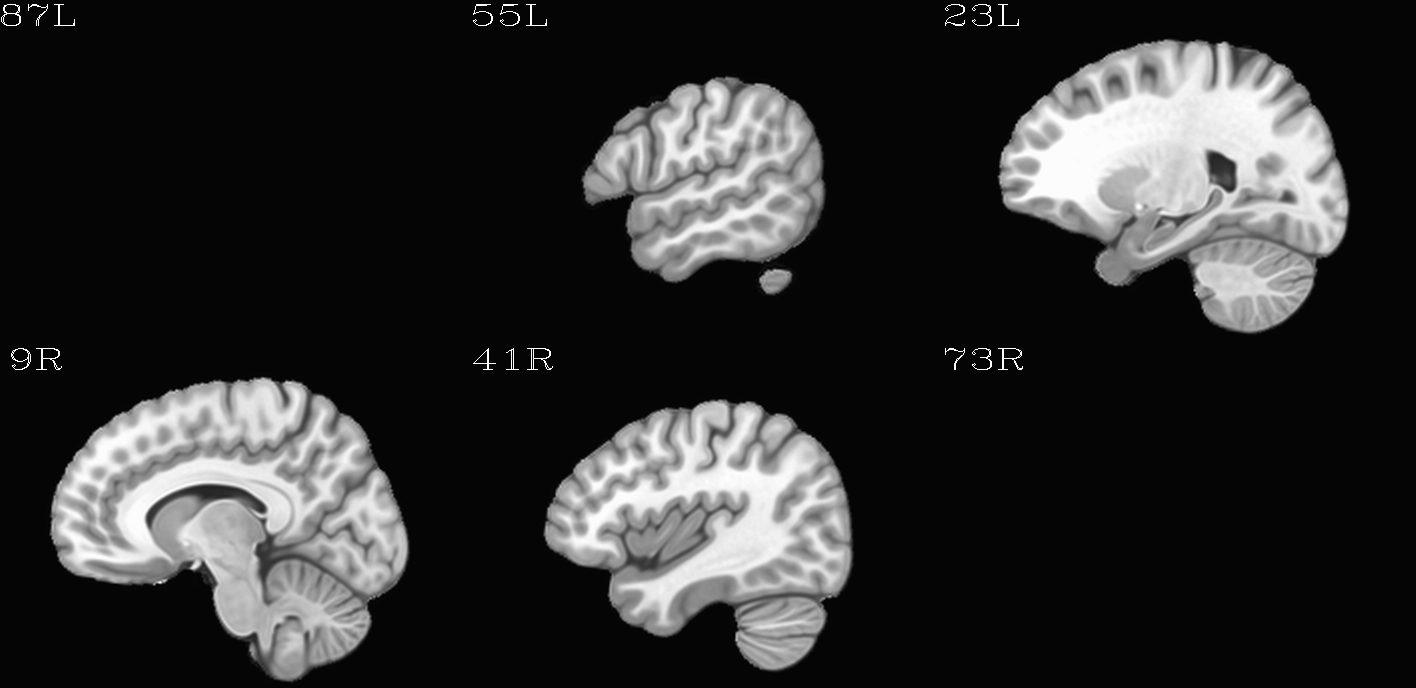
For the purposes of axialization, it is necessary to have a reference volume that has desired orientation within a FOV. In this example we are looking at an adult human dset, which includes a T2w volume for reference within TORTOISE processing. Therefore, we want to have a reference volume with T2w contrast.
We started by downloading the “ICBM 2009a Nonlinear Symmetric”
atlases
freely available for download from the BIC folks at MNI. One
volume was manually AC-PC aligned by an expert using MIPAV, and the
other volumes were registered to it. (During this process, the FOV of
the data was altered– the resulting volume has an even number of
slices in all directions.) The volumes were masked to remove the
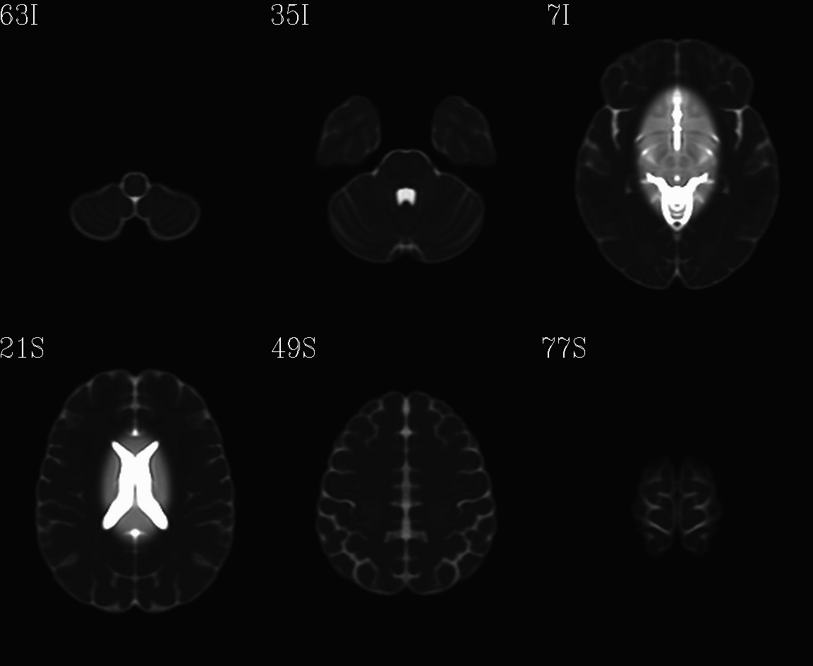
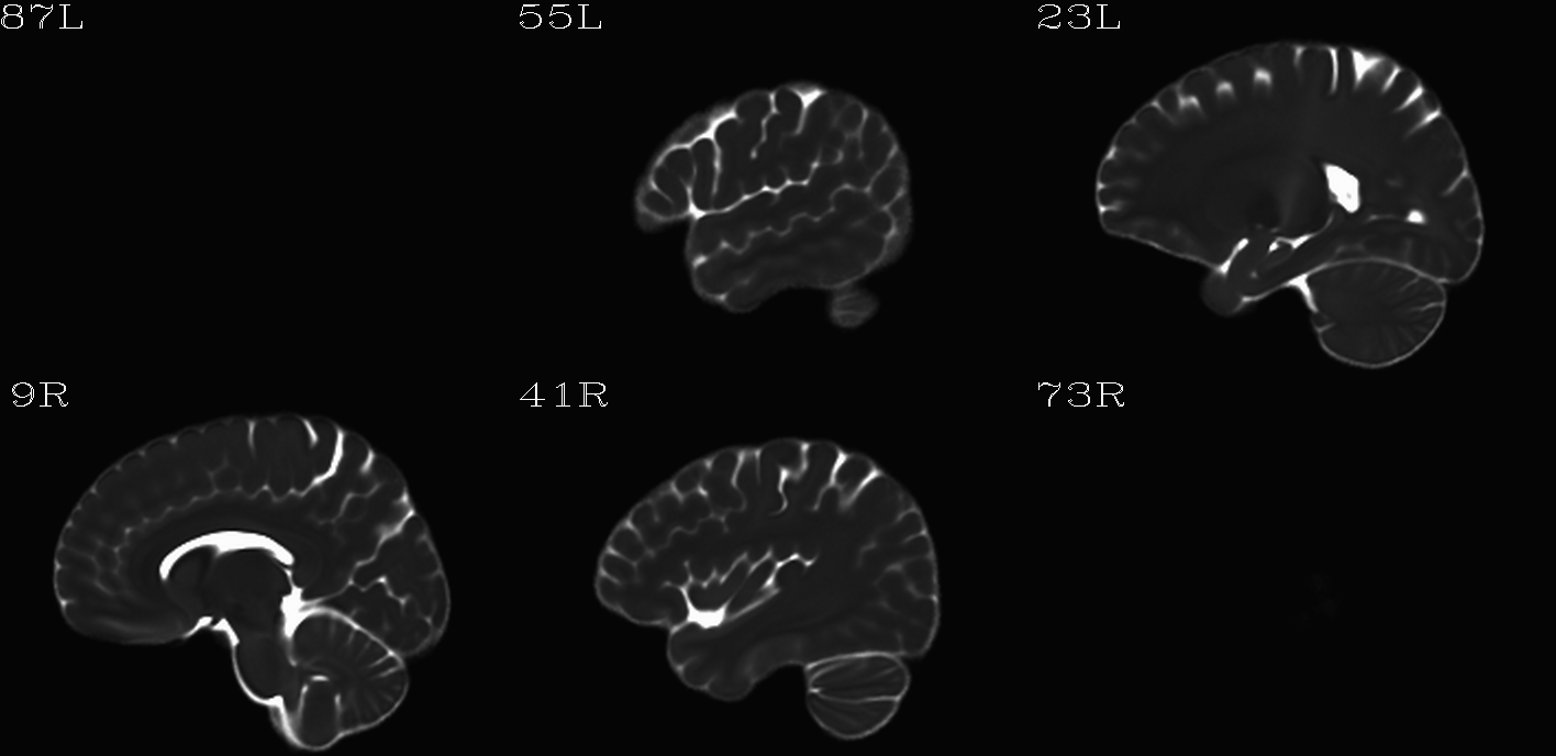
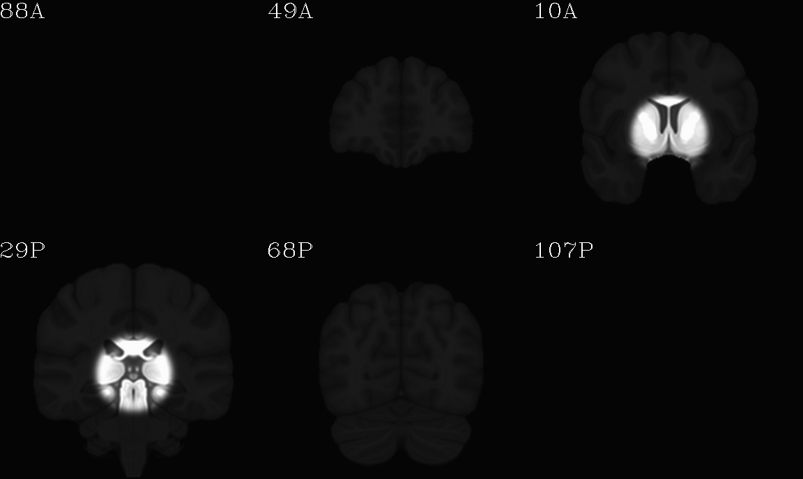
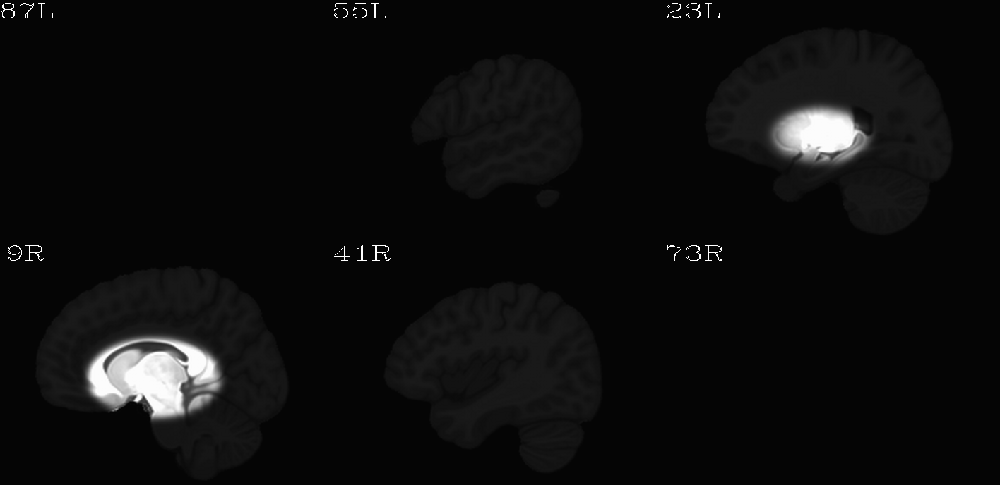
skull. Finally, a subcortical weight mask version of each volume was
also made by weighting (values  ) a blurred ellipsoid
covering much of the subcortical brain; using this mask would weight
the global brain alignment by this part of the brain, with the idea
that the final result of axialization might be closer to what AC-PC
alignment would provide. This was done for the T2w and T1w volumes in
the MNI set, which are shown below and can be downloaded from here on
the AFNI website.
) a blurred ellipsoid
covering much of the subcortical brain; using this mask would weight
the global brain alignment by this part of the brain, with the idea
that the final result of axialization might be closer to what AC-PC
alignment would provide. This was done for the T2w and T1w volumes in
the MNI set, which are shown below and can be downloaded from here on
the AFNI website.
T2w reference volume |
T2w (subcortical) weight mask |
|---|---|
mni_icbm152_t2_relx_tal_nlin_sym_09a_ACPCE.* |
mni_icbm152_t2_relx_tal_nlin_sym_09a_ACPCE_wtell.* |
|
|
|
|
|

|
T2w volume (originally from MNI ICBM 2009a Nonlinear Symmetric atlas) used as a reference for axialization. |
The subcortical weight mask of the T2w reference volume, emphasizing the subcortical region. |
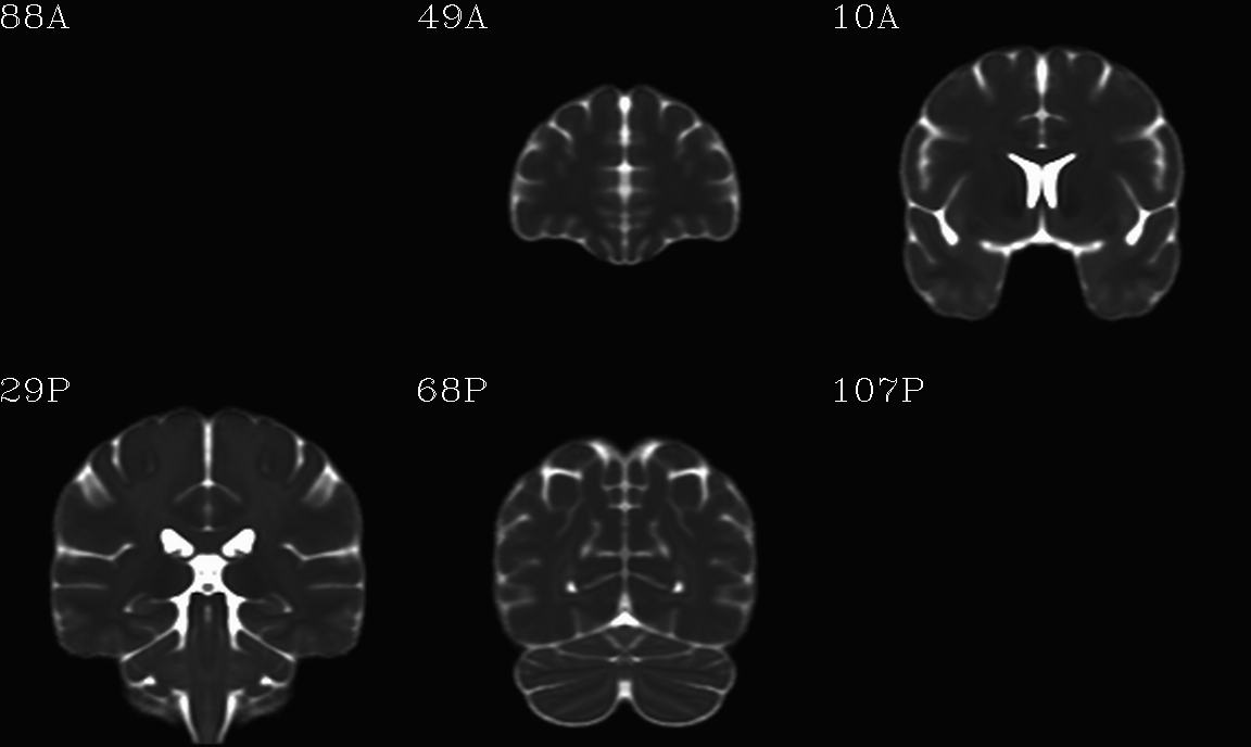
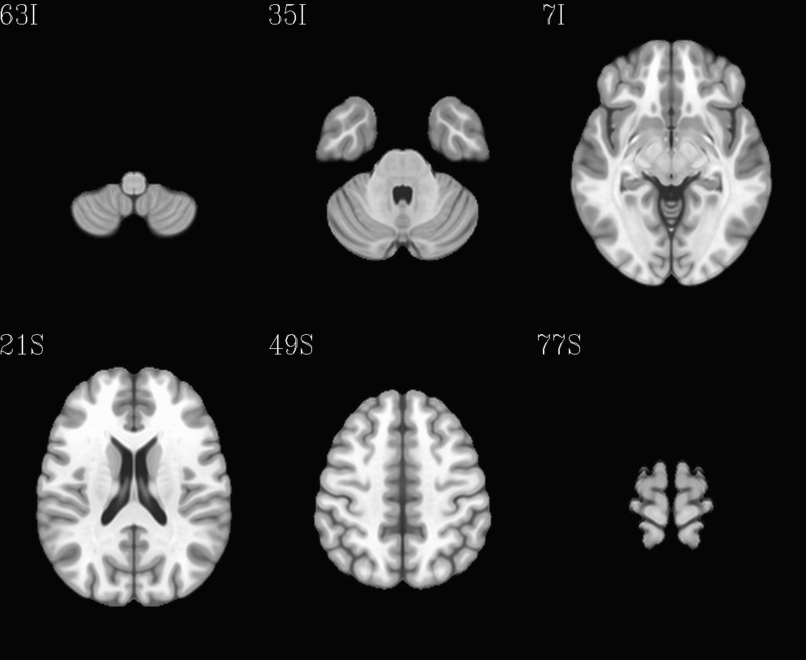
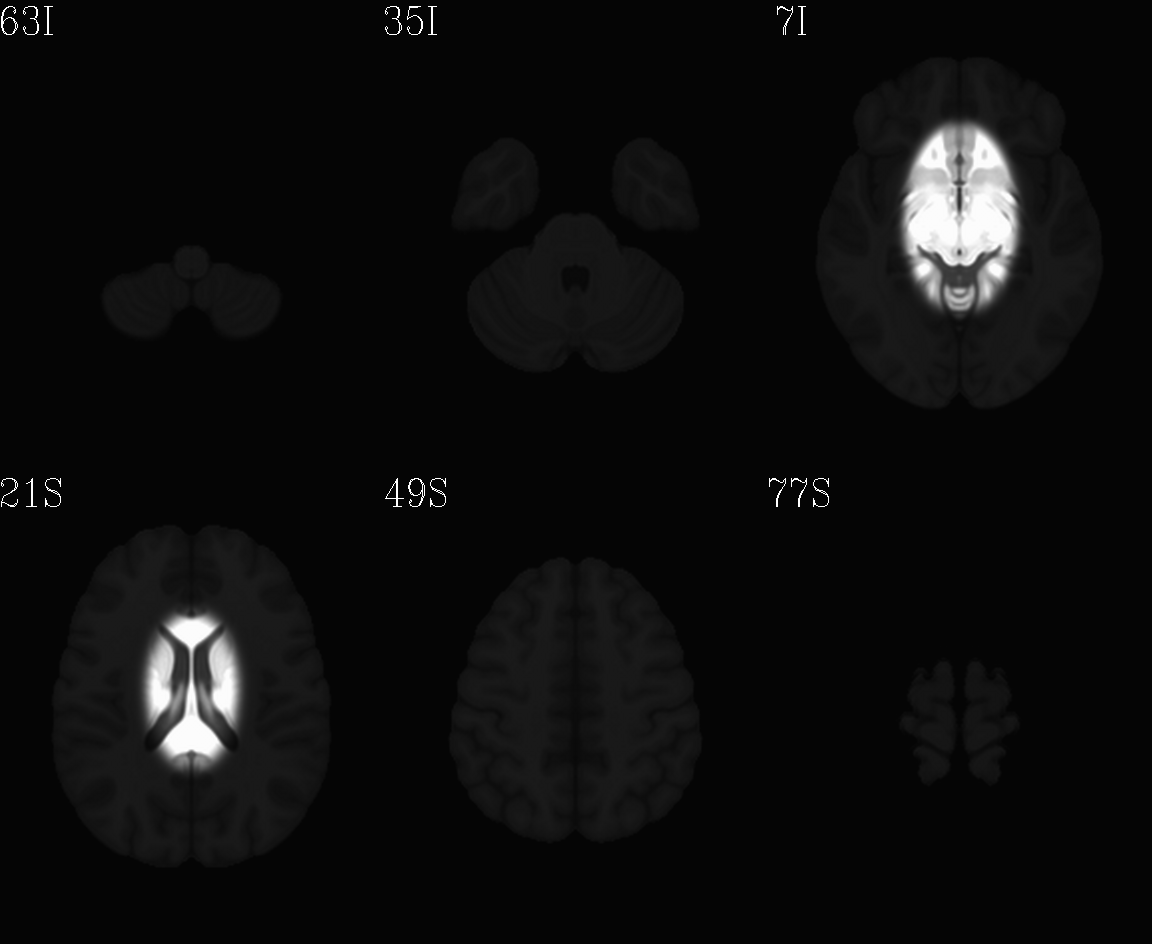
T1w reference volume |
T1w (subcortical) weight mask |
|---|---|
mni_icbm152_t1_relx_tal_nlin_sym_09a_ACPCE.* |
mni_icbm152_t1_relx_tal_nlin_sym_09a_ACPCE_wtell.* |
|
|
|
|
|
|
T1w volume (originally from MNI ICBM 2009a Nonlinear Symmetric atlas) used as a reference for axialization. |
The subcortical weight mask of the T1w reference volume, emphasizing the subcortical region. |
Note
Both axialization and AC-PC alignment have similar goals of “regularizing” the orientation of a brain within a field of view. However, please note that they are not the same thing. The AC-PC alignment criterion is based on identifying 5 specific local, anatomical locations in the brain and using these to lever the brain orientation. Axialization is based on a global, whole brain alignment of brain structures (with the possible addition of a weight mask to emphasize certain parts of the structure).
In many cases, such as for typical/control brains, the results of either regularization may be very similar. However, there would be many scenarios where results would differ, and the user must choose what is most appropriate and/or feasible for their own study.
Distorted views of the DWI world
What do distortions in DWI data look like? Ugly stuff.
EPI distortion
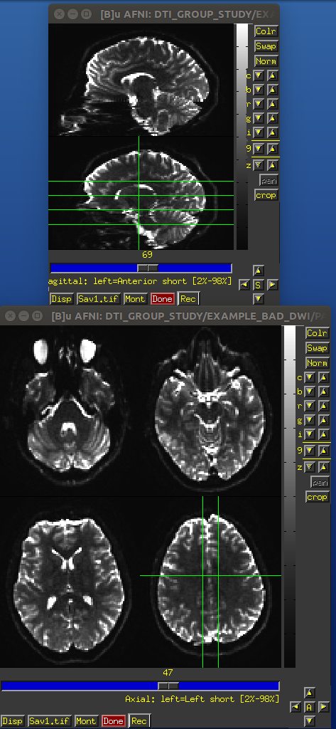
EPI distortions occur predominantly along the phase encode direction (often along the anterior-posterior orientation), and these cause both geometric distortions (brain warping: stretching and compressing) and signal intensity distortions (wrong signal value stored: signal pileup and attenuation). These can effect both the reference b =0 and gradient weighted volumes.
One can see the relative the locations of greatest distortion when comparing the oppositely phase encoded data. TORTOISE uses registration between the oppositely encoded sets, as well as the anatomical reference, to reduce the warping distortions (see Irfanoglu et al., 2012).
Identical slices, single subject DWI.
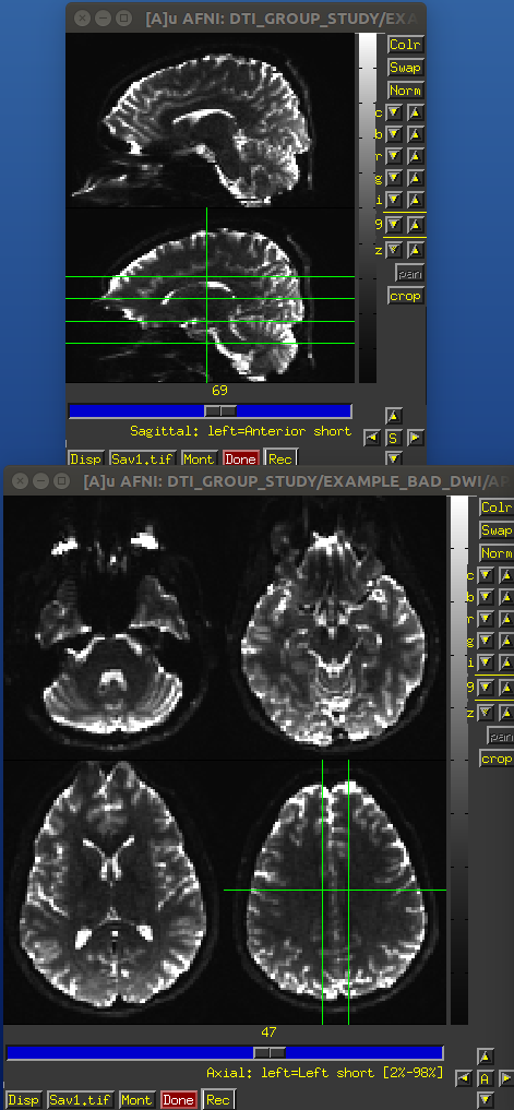
PA encoded b=0 volume.
AP encoded b=0 volume.
Eddy current distortion
Rapid switching of the diffusion gradients causes distortions. These occur in the b>0 volumes of a DWI data set. They cause nonlinear distortions, and generally need nonlinear registration to reduce their effects. The
DIFFPREPpart of TORTOISE tries to undo some of these.Subject motion
When we talk about subjection motion, we can talk about two main types: motion occuring between volumes, and motion that occurs with a TR. (And in practice, there is often a combination of the two.) If motion happened only between TRs, then we are in a better position to “correct” some of its effects, essentially by using a good volume registration procedure. The assumption is that the signal value at a location is what it should be– we just have to reorient the head to put that voxel back where it was pre-motion. (NB: this is a simplification– motion has other knock-on effects on data acquisition, but we hope these are fairly small.)
The within-TR motion is quite problematic, though. Consider a standard DWI acquisition sequence that collects axial slices in an interleaved pattern. That is, it collects slices #0, 2, 4, 6, 8, etc. and then slices #1, 3, 5, 7, etc. What happens if a person moves during this? Pre-motion slices might be fine, but those afterward are not properly measured, and a distinctive brightness pattern can be seen in a sagittal view. This is often known as the “Venetian blind” effect, and it is very easy to spot when looking at data– this would be a good candidate to filter out.
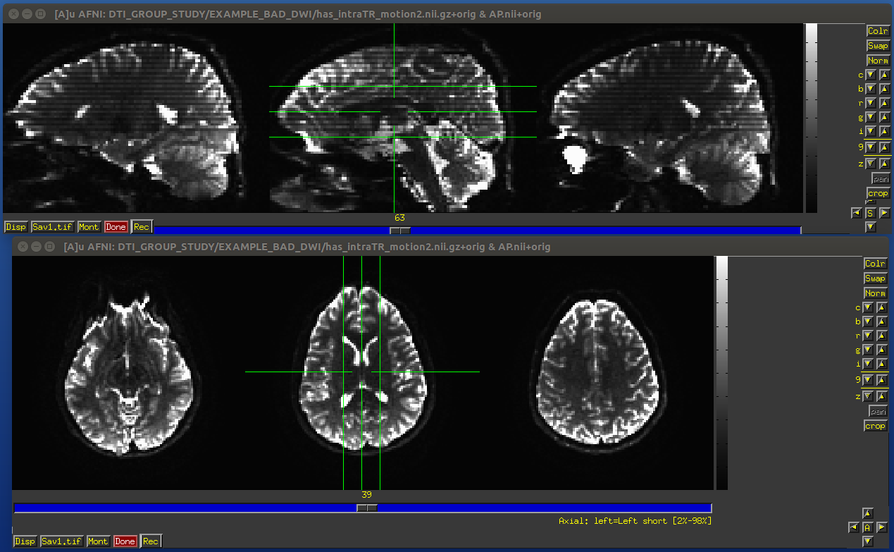
Example of subject motion artifact in a DWI volume that was acquired with an interleaved sequence (which is common).
Signal dropout
Signal dropout can occur due to susceptibility and excitation problems, sometimes limiting problems to just one slice. However, that slice is effectively useless, and one might consider filtering out this volume. (NB: in some cases, the volume could be left in if using an outlier rejection algorithm on a voxelwise basis for tensor fitting.)
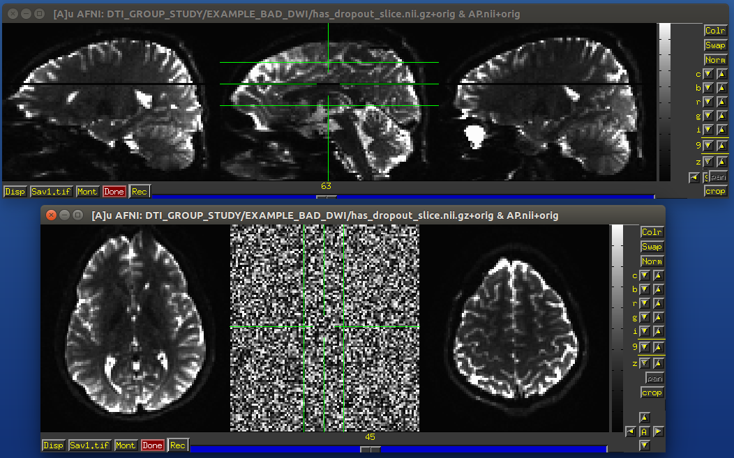
Example of a dropout slice in a DWI volume.


