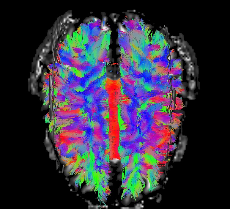
12.5.7. Post-preproc, I: tensor estimation and checking
Overview
Now we want to estimate the diffusion tensors (DTs) and DT parameters. There are additional considerations:
After TORTOISE processing, the DWIs overlay on the reference anatomical, but this volume itself generally has a different grid, (resolution, origin and orientation) from the originally input volume (where other things like a T1w volume, etc. might already have been aligned). Therefore, too keep our volumes overlaying as much as possible, we move both the reference structural.nii and DWI volume to overlay the originally input T2w reference volume.
There is a fun phenomenon in DWI acquisition + processing, that scanner vendors and various softwares somehow often have different meanings to gradient orientations along a volume’s FOV: for example, for the x-coordinate, is a positive value in the right or left direction? (and so forth for each component). This is known as the “gradient flipping” problem, and I have whined about it voluminously in “How to check about gradient flipping?”. Here, we briefly discuss using
@GradFlipTestto check things as part of a pipeline and demonstrate how it can be incorporated into scripts (with cautionary notes for doing so!).We might find it interesting to estimate the uncertainty of some DTI parameters in preparation for either full probabilistic or mini-probabilistic tracking. (If the implications of either of terms are unfamiliar, then perhaps check out more information about FATCAT tracking options in “3dTrackID: making tracts”.
On a mundane note, the physical scale of many scalar DTI parameters is pretty small, for example having
. Having such tiny numbers can lead to annoyances during analysis, for example with their even smaller differences and floating point precision. Therefore, instead of having “small number” in units of
, we find it more convenient to have “number of order unity” in units of “
”, which is totally legit, too.
Re. @GradFlipTest
The primary documentation for @GradFlipTest is provided on this
page, “@GradFlipTest: checking on gradient flips”.
In brief, if you do not know whether and/or how the gradients in your
data set should be “flipped” in order to be consistent with processing
in AFNI (every software and scanner/vendor might be using different
systems, oddly enough), then you can use @GradFlipTest to guess
what is right. The tool uses whole brain tracking under all possible
gradient flip configurations to hypothesize a relevant flip (including
no-flip) for the data set at hand. It also produces commands to view
your results in SUMA to double check. Note the caveats with blindly
including this in scripts without checking (-> though, in truth,
every step should be checked without blindly trusting!).
In the usage example of fat_proc_dwi_to_dt, below, we show how
@GradFlipTest can be incorporated into a pipeline directly.
fat_proc_dwi_to_dt (+ @GradFlipTest)
At the end of the DWI preprocessing step, there may be several data
sets that are in various “spaces” (i.e., with different grids), and,
particularly if non-AFNI software is being used, things like the FOV,
origin and orientation of data may have been changed. In short, there
may be several data sets that 1) don’t overlap with each other and 2)
don’t overlap with the data originally entered, even though they
probably should. This happens, for example, when using TORTOISE (see
the description of outputs in this section,
“DR_BUDDI”; it similarly happens when only
DIFFPREP is used, as well). Esp. since TORTOISE aligns DWIs to
the reference anatomical volume, there is no reason that the data
shouldn’t overlay with the anatomical originally entered (and to which
other data, such as a T1w volume and FreeSurfer output, may also be
aligned). For convenience, fat_proc_dwi_to_dt can help the
processed data sets align with the original anatomical (to the degree
that the data itself allows) by simply adjusting the origins and
orientations.
During the tensor fitting stage, several useful options are switched
on for 3dDWItoDT:
using nonlinear alignment via
-nonlinear, essentially default for primary tensor fittingperforming an extra round of tensor fitting with
-reweighting, and the cumulative weight values are output with-cumulative_wtsscaling physical measures conveniently via
-scale_out_1000, so numerical values aren’t tiny (for adult humans)– units are in “”
calculating chi-square results via
-debug_briks, for goodness-of-(tensor)-fit measuresmasking via the anatomical, which hopefully has more “clarity” and less brightness inhomogeneity than the DWI volumes themselves
Additionally, uncertainty values of DTI parameters are calculated with
3dDWUncert, for use with tracking in 3dTrackID.
QC images are also output. The DWI volume is shown
overlayed and edge-ified on the reference anatomical are made, as well
as thresholded FA maps (FA>0.2, for the standard proxy of DTI-defined
WM maps in healthy adult humans; alterable for other cases).
Proc: Processing in this case involves two steps: A) use the DWIs b-matrix gradient info to estimate what flip is necessary to make those data pieces consistent for AFNI; and B) make the DWI output overlay on the original input T2w volume well, and then add in the b-matrix (with any necessary flip) to estimate the DT and associated parameters. Step “B” involves using both the pre- and post-TORTOISE anatomical reference file; NB: one doesn’t have to include these anatomical files, but if you are using TORTOISE (as we are here) then you really should. Also, masking of DWIs to find the brain can be problematic due to brightness inhomogeneities, etc., so using the structural image for this aspect is also beneficial (though not guaranteed to be perfect). Therefore, one can run:
# I/O path, same as above, following earlier steps
set path_P_ss = data_proc/SUBJ_001

# shortcut names for what will be our input (-> from TORT proc)
# and output (-> another dwi_* directory)
set itort = $path_P_ss/dwi_04
set odir  = $path_P_ss/dwi_05

# A) do autoflip check: not ideal to need this, but such is life
@GradFlipTest \
    -in_dwi       $itort/buddi.nii                \
    -in_col_matT  $itort/buddi.bmtxt              \
    -prefix       $itort/GradFlipTest_rec.txt

# get the 'recommended' flip; still should verify visually!!
set my_flip = `cat $itort/GradFlipTest_rec.txt`

# B) DT+parameter estimates, with flip chosen from @GradFlipTest
fat_proc_dwi_to_dt \
    -in_dwi       $itort/buddi.nii                    \
    -in_col_matT  $itort/buddi.bmtxt                  \
    -in_struc_res $itort/structural.nii               \
    -in_ref_orig  $path_P_ss/anat_01/t2w.nii          \
    -prefix       $odir/dwi                           \
    -mask_from_struc                                  \
    $my_flip
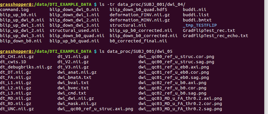
-> putting the flip-test files and directory into the existing+populated ‘data_proc/SUBJ_001/dwi_04/’, and the DT and parameters into ‘data_proc/SUBJ_001/dwi_05/’:
Directory substructure for example data set |
|---|
|
Output from @GradFlipTest and fat_proc_dwi_to_dt. |
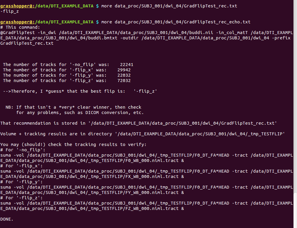
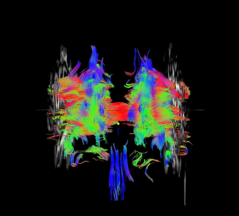
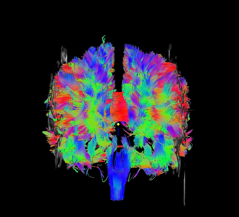
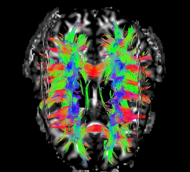
Part A: @GradFlipTest output. Note that only the last three files in ‘*/dwi_04/’ (Grad* and _tmp*/) were made by @GradFlipTest.
Outputs of |
|
|---|---|
GradFlipTest_rec_echo.txt |
textfile, with a record exact command that was run at the top;
importantly, it also contains the number of tract counts that
lead to the program’s flip guess as well as |
GradFlipTest_rec.txt |
textfile, simply the “best guess” of flip (one of: |
_tmp_TESTFLIP/ |
“working” directory for the script, but also contains the tracked outputs for each tested flip; the user can use command calls from the “Grad*echo.txt” file to view the relative whole brain trackings and thereby judge whether the function’s guess should be used or not. |
Note
Something that can happen at this step to be aware of: in
@GradFlipTest, the default method for making the whole
brain mask within which to perform tracking is simple
automasking of the DWI’s [0]th volume. This may not be
great, both missing out parts of the brain (esp. if there
are large brightness inhomogeneities across the volume) or
including skull, non-brain tissue etc. depending on the
image. A separate mask could be made by the user an input,
if necessary.
If you look closely, you can see that this has even happened in the above case: in the cor view, a gap in tracts is visible inferior to the corpus callosum. This occured because the volume for automasking has large dark regions. However, the remaining mask provided enough coverage for guessing what flip would be appropriate. Such are the judgments users need to make– and another reason to look at your data!!
... and with the flip guessed, we can then continue on to the actual tensor fitting et al.
Part B: fat_proc_dwi_to_dt. All of the output from
fat_proc_dwi_to_dt in ‘*/dwi_05/’ should overlay the original T2w
reference that was input into TORTOISE.
Outputs of |
|
|---|---|
dwi_cmd.txt |
textfile, copy of the command that was run, and location |
dwi_dwi.nii.gz |
volumetric NIFTI file, 4D (M=31 volumes) |
dwi_bvec.txt |
textfile, column file of (DW scaled) b-vectors ( |
dwi_bval.dat |
textfile, column file of M b-values |
dwi_matA.dat |
textfile, column file of (DW scaled) AFNI-style b-matrix
( |
dwi_anat.nii.gz |
volumetric NIFTI file, 3D; structural output by TORTOISE that was aligned with DWIs and had same spatial resolution; it was used to align to the initial T2w reference, and should be aligned with that and the dwi_dwi.nii.gz file. |
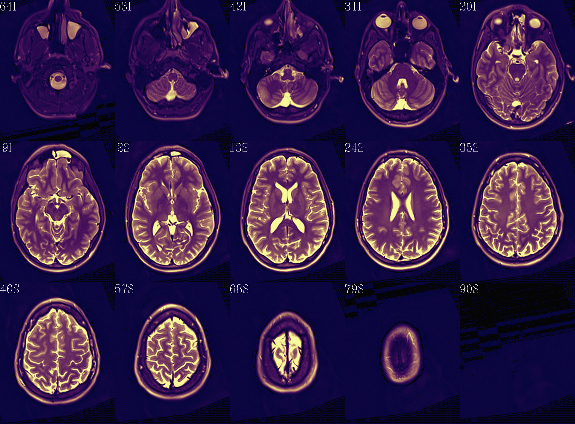
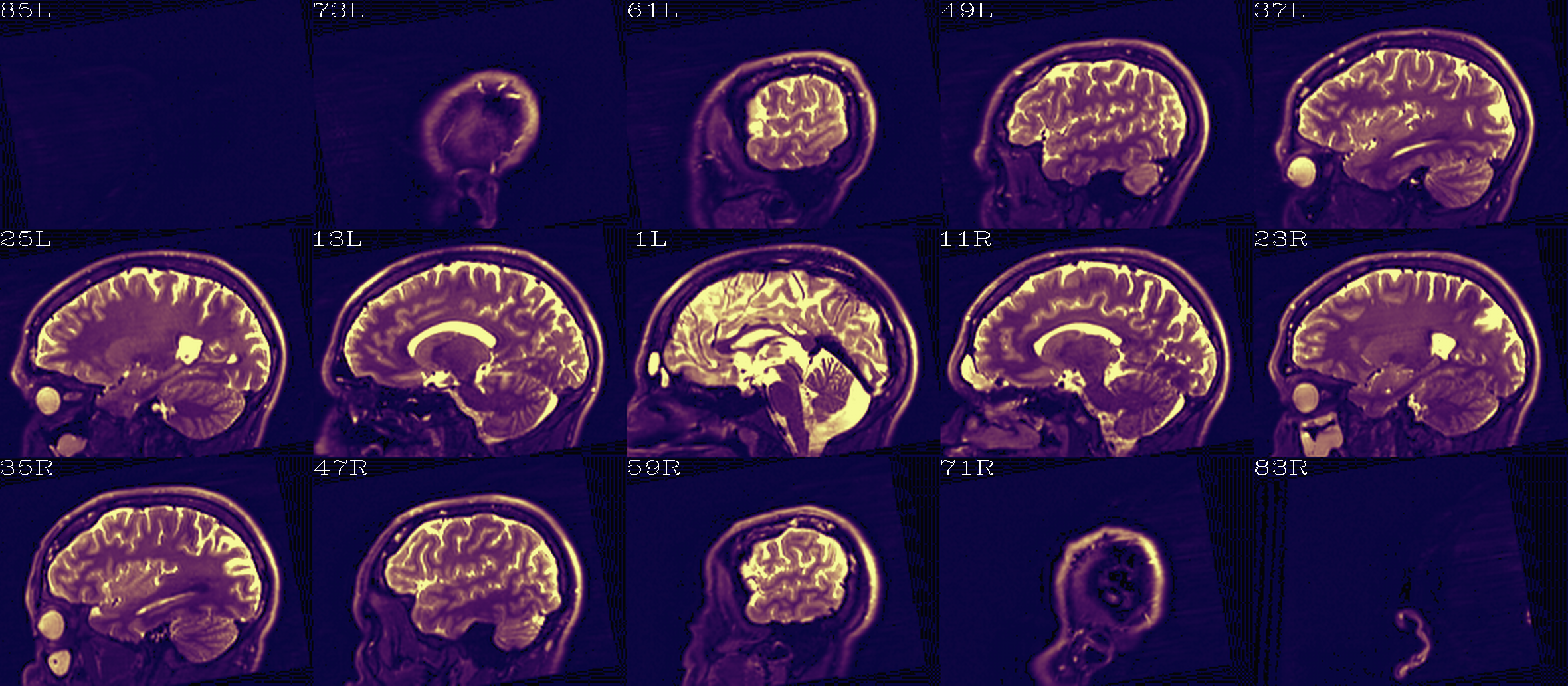
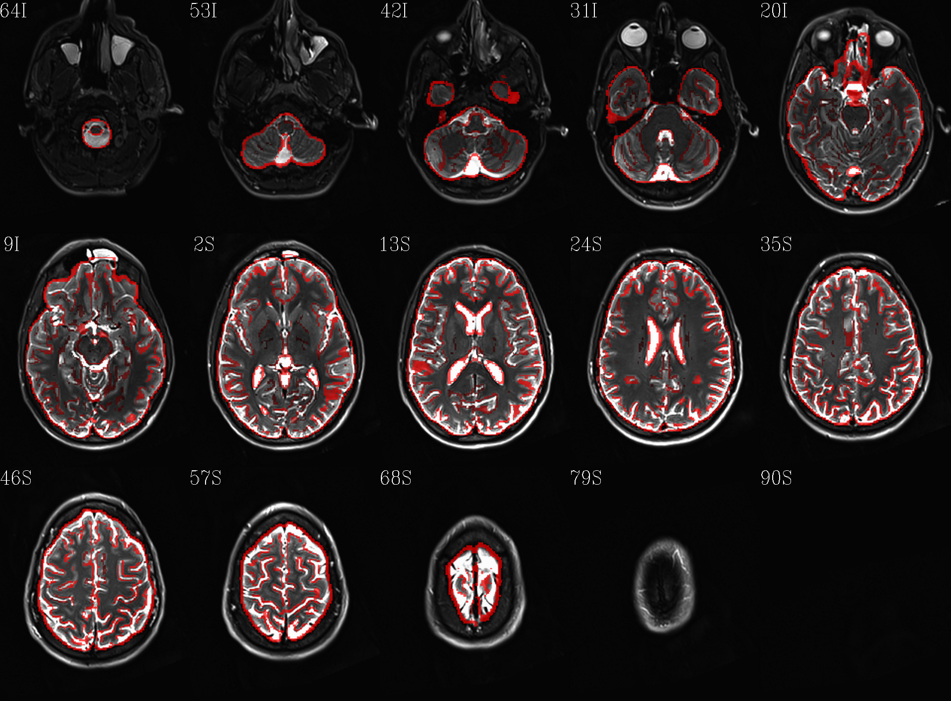
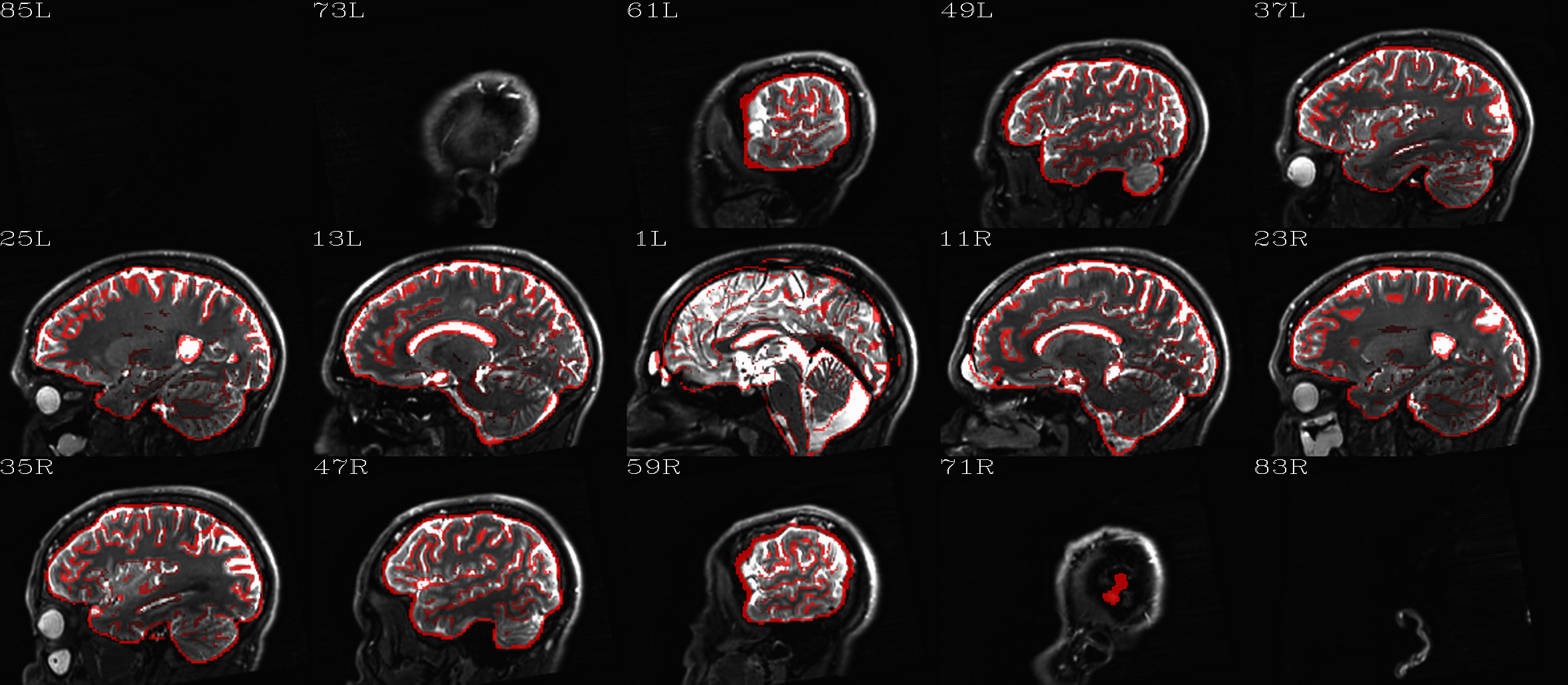
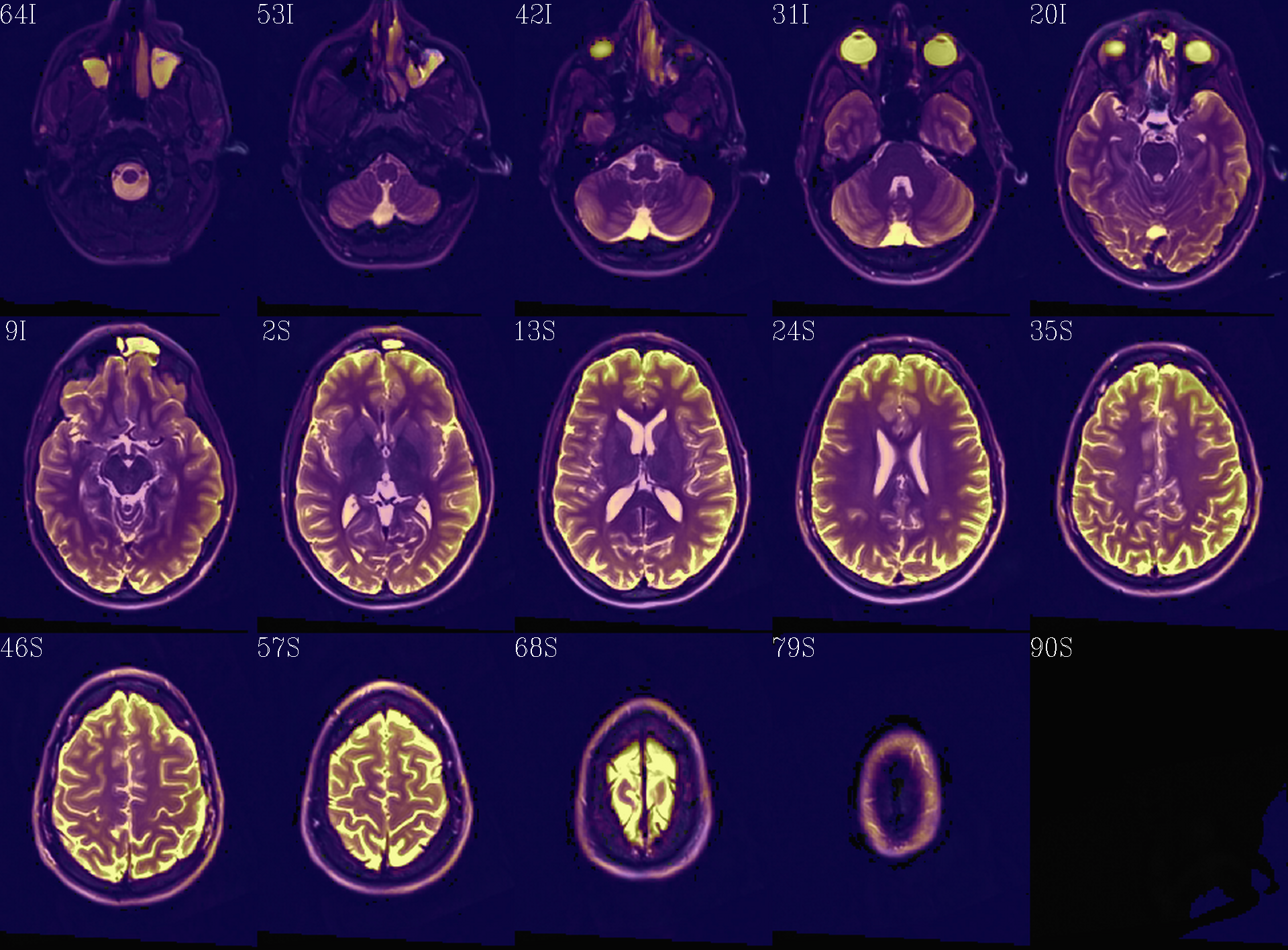
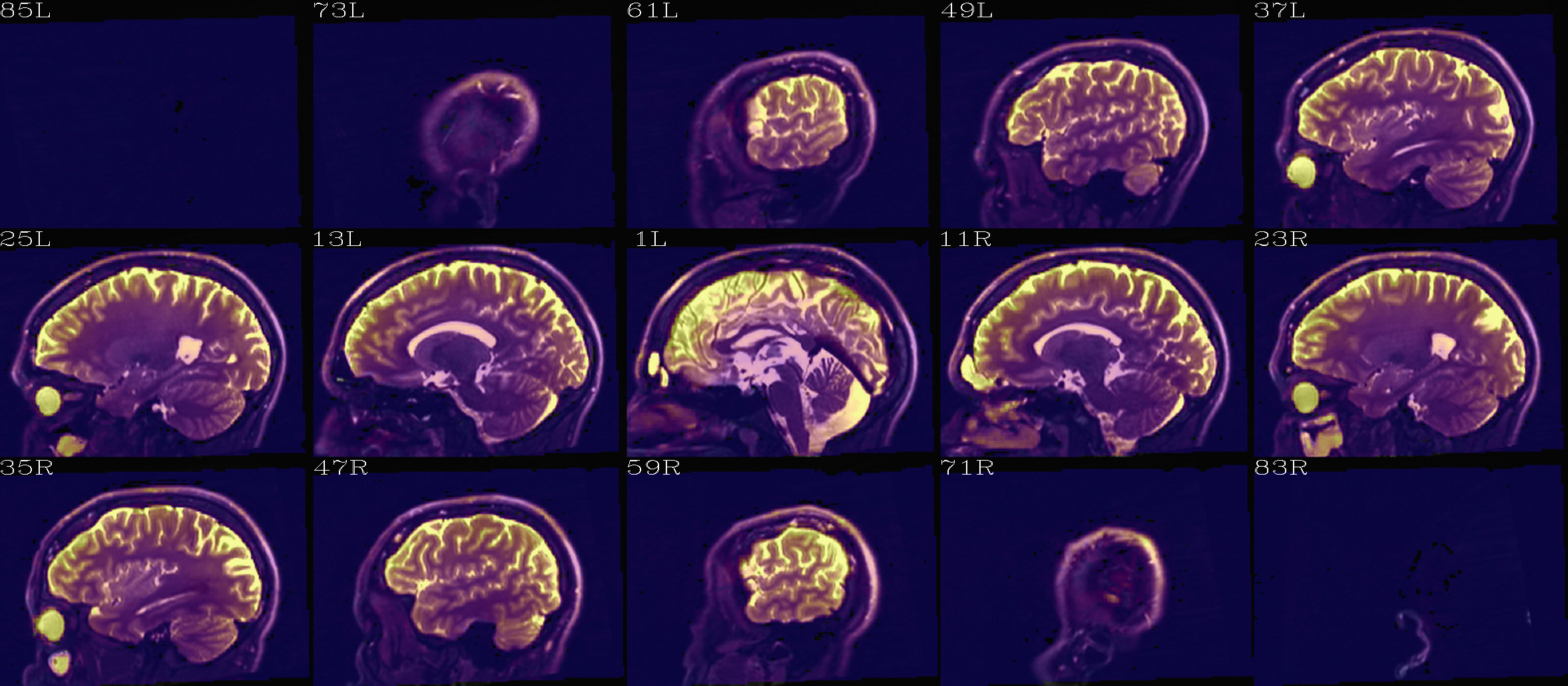
dwi__qc00_ref_u_struc.*.png |
autoimages, multiple slices within single volume; ulay = reference T2w anatomical that was input into TORTOISE (b/w); olay = dwi_anat.nii.gz, which was structural.nii file output by TORTOISE (translucent with ‘plasma’ colorbar). Should match very well. |
dwi__qc01_ref_u_eb0.*.png |
autoimages, multiple slices within single volume; ulay = reference T2w anatomical that was input into TORTOISE (b/w); olay = edge-ified dwi_dwi.nii.gz[0]. Use this image to check TORTOISE alignment of DWIs with reference anatomical. Very useful! |
dwi__qc02_ref_u_b0.*.png |
same as *qc01*png, but the olay is the full dwi_dwi.nii.gz[0] with translucent-‘plasma’ coloration. Probably the edge-ified one is more useful. |
dwi_mask.nii.gz |
volumetric NIFTI file, 3D; mask made by (here) automasking
|
dt_*.nii.gz |
volumetric NIFTI files from |
dt_cwts.1D |
text file, column of M numbers, the cumulative weights for each gradient volume. |
dwi__qc03_MD_u_FA_thr0.2.*.png |
autoimages, multiple slices within single volume; ulay = mean diffusivity from tensor fit (b/w); olay = FA volume thresholded at >0.2 (‘plasma’ colorbar). |
Autoimages of |
(just axi and sag views) |
|---|---|
|
|
Aligment of post-TORTOISE reference anatomical (translucent olay) with pre-TORTOISE one (b/w ulay); should be very good fit. |
|
|
Aligment of DWI [0] volume (edge-ified olay) with pre-TORTOISE one (b/w ulay); useful judge of processing alignment, distortion correction, etc. |
|
|
Aligment of DWI [0] volume (translucent olay) with pre-TORTOISE one (b/w ulay); useful judge of processing alignment, distortion correction, etc. |
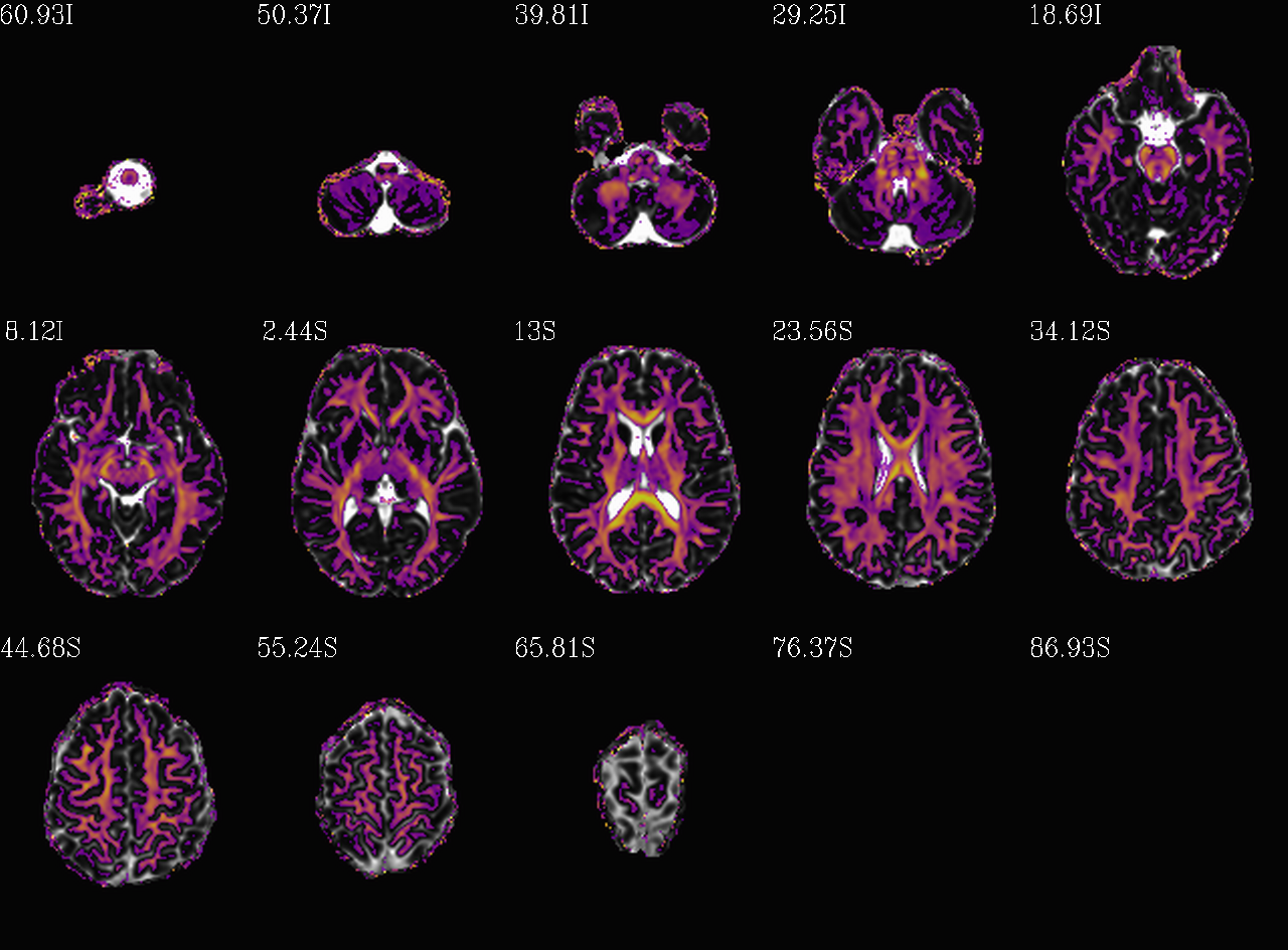
|
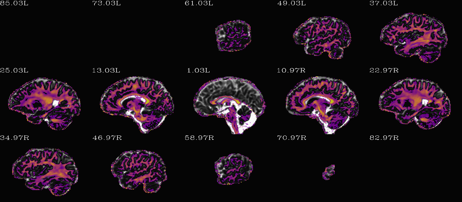
|
Thresholded FA>0.2 map (olay) on MD (b/w ulay); check for full coverage, lack of abormalities, etc. |
fat_proc_decmap
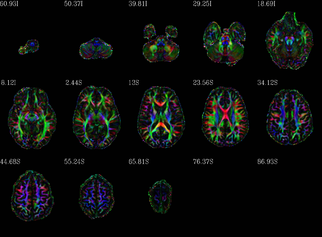
Another useful kind of image for investigating DT data is the DEC
(directionally-encoded color) map. In DTI the first eigenvector (“V1”)
provides the main orientation of interest in a voxel; in a DEC map,
the components of that 3D vector are converted into
an RGB (red-green-blue) coloration for that voxel. FA values can be
used to scale the brightness. The coloration shows the relative
degree that a vector is oriented along a major axis:
red : left <-> right,
blue : inferior <-> superior,
green : anterior <-> posterior.
Here, the unweighted DEC map dset is calculated and the viewed in different forms:
- Standard DEC. RGB from V1 and brightness scaled by FA:
.
- Unweighted DEC. RGB from V1 and no brightness scaling:
.
- Scaled (weighted) DEC. RGB from V1 and scaled by FA, which itself is weighted by some value SS:
.
This might be useful in cases where the volume looks “too dark” for standard FA brightness scaling. In the present example, we usesince that is an “upper percentile” value (and it probably would be in much of DTI).
Note
As you might notice by the definition of V1-to-RGB calculations, the coloration of a structure will depend on how it is “aligned” with respect to the dset’s FOV. This is one major reason why we want to have an “axialized” (or “AC-PC” aligned) dset for analysis– so we can expect fairly consistent coloration across subjects.
Proc: The inputs are pretty basic. All that is needed are the first eigenvector (“V1”) and fractional anisotropy (“FA”) volumes, with an optional mask:
# I/O path, same as above, following earlier steps
set path_P_ss = data_proc/SUBJ_001

fat_proc_decmap                                     \
    -in_fa       $path_P_ss/dwi_05/dt_FA.nii.gz     \
    -in_v1       $path_P_ss/dwi_05/dt_V1.nii.gz     \
    -mask        $path_P_ss/dwi_05/dwi_mask.nii.gz  \
    -prefix      $path_P_ss/dwi_05/DEC
-> putting the DEC map volume and images into ‘data_proc/SUBJ_001/dwi_05/’:
Directory substructure for example data set |
|---|
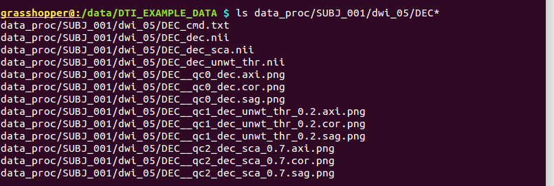
|
Output from fat_proc_decmap. |
While having the NIFTI volumes might be useful, the main point of the
fat_proc_decmap function is really to make these quickly visible
PNG images.
Outputs of |
|
|---|---|
DEC_cmd.txt |
textfile, copy of the command that was run, and location |
DEC_dec.nii |
volumetric NIFTI file, 3D volume of the ‘rgb’ datum type; unscaled DEC map. |
DEC_dec_sca.nii |
volumetric NIFTI file, 3D volume of the ‘rgb’ datum type; DEC map scaled by FA value. |
DEC_dec_unwt_thr.nii |
volumetric NIFTI file, 3D volume of the ‘rgb’ datum type; DEC map unweighted/scaled, but thresholded where FA>0.2. |
DEC__qc0_dec.*.png |
autoimages, multiple slices within single volume; the “standard” DEC map: V1-to-RGB with FA scaling.* |
DEC__qc1_dec_unwt_thr_0.2.*.png |
autoimages, multiple slices within single volume; the “unscaled” DEC map: V1-to-RGB with no scaling, but also thresholded where FA>0.2.* |
DEC__qc2_dec_sca_0.7.*.png |
autoimages, multiple slices within single volume; the “scaled+weighted” DEC map: V1-to-RGB with FA scaling, but the FA value itself is scaled (here, with a scale of 0.7).* |
Autoimages of |
(just axi and sag views) |
|---|---|
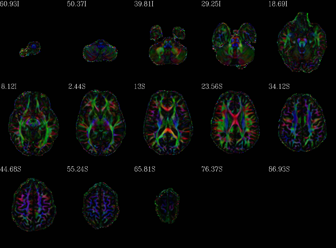
|
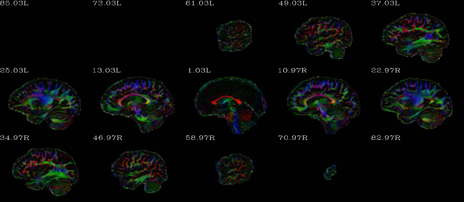
|
“Standard” DEC map, scaled by FA. |
|
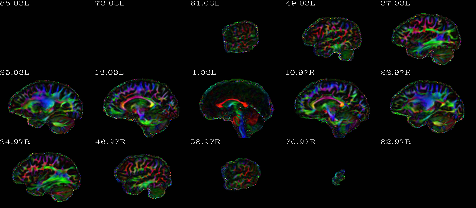
|
DEC map scaled by FA, but that FA itself is weighted/scaled by FA=0.7 (so it is a bit brighter than the “standard” one). |
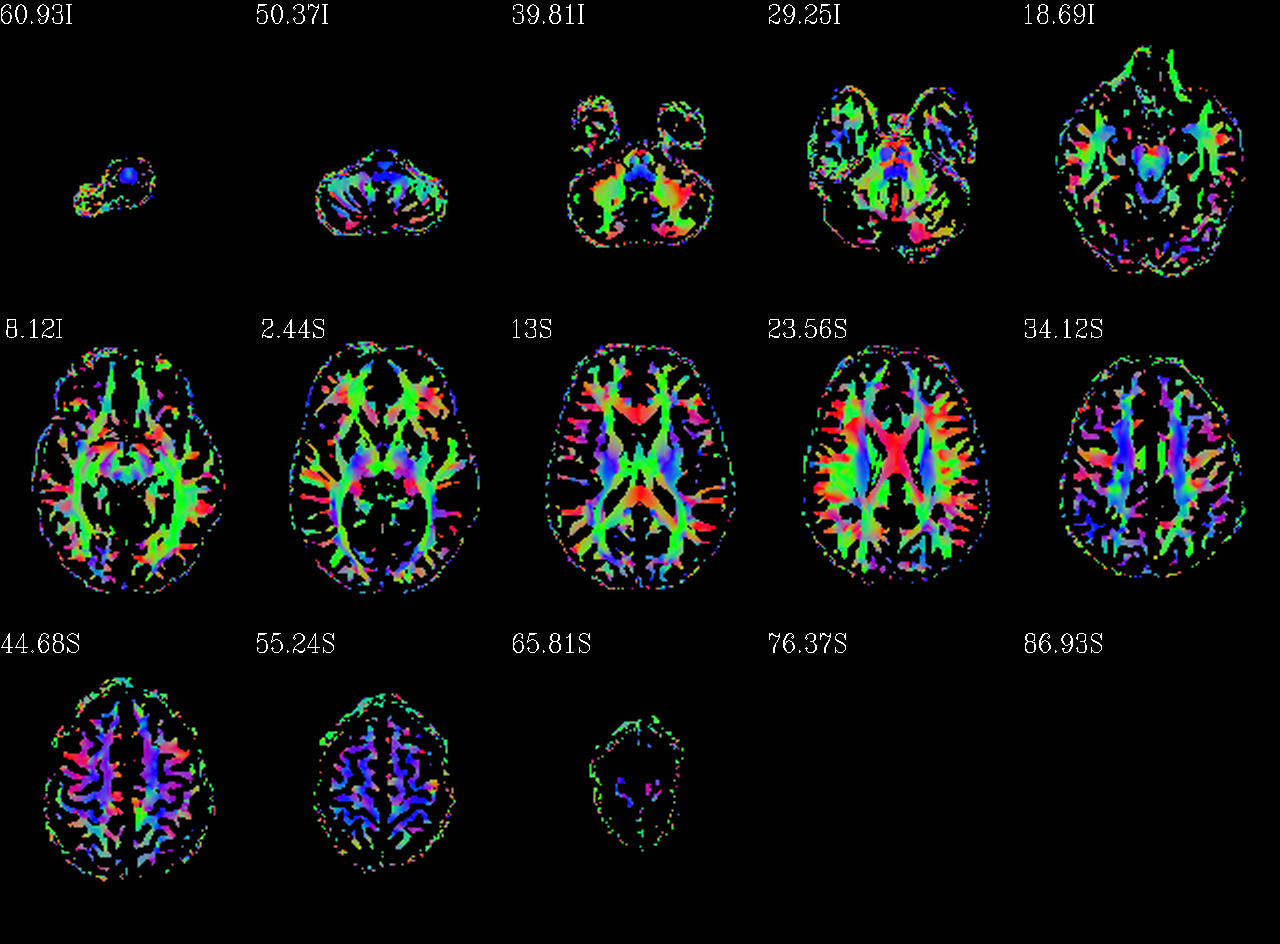
|
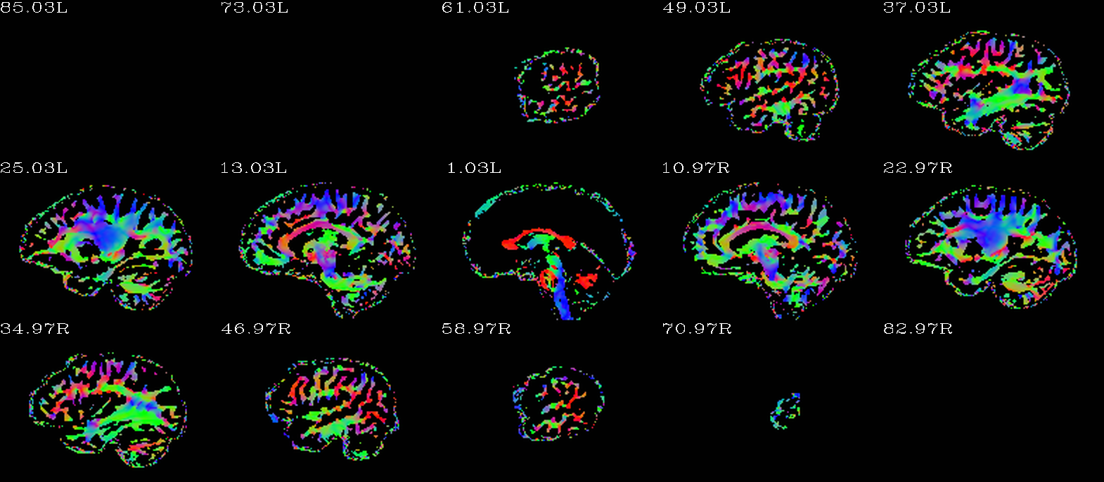
|
Unscaled DEC map, thresholded where FA>0.2. |
