All AFNI program -help files
This page auto-generated on Mon Jul 6 11:24:44 PM EDT 2026
AFNI program: 1dApar2mat
Usage: 1dApar2mat dx dy dz a1 a2 a3 sx sy sz hx hy hz
* This program computes the affine transformation matrix
from the set of 3dAllineate parameters.
* The result is printed to stdout, and can be captured
by Unix shell redirection (e.g., '|', '>', '>>', etc.).
See the EXAMPLE, far below.
* One use for 1dApar2mat is to take a set of parameters
from '3dAllineate -1Dparam_save', alter them in some way,
and re-compute the corresponding matrix. For example,
compute the full affine transform with 12 parameters,
but then omit the final 6 parameters to see what the
'pure' shift+rotation matrix looks like.
* The 12 parameters are, in the order used on the 1dApar2mat command line
(the same order as output by 3dAllineate):
x-shift in mm
y-shift in mm
z-shift in mm
z-angle (roll) in degrees (not radians!)
x-angle (pitch) in degrees
y-angle (yaw) in degrees
x-scale unitless factor, in [0.10,10.0]
y-scale unitless factor, in [0.10,10.0]
z-scale unitless factor, in [0.10,10.0]
y/x-shear unitless factor, in [-0.3333,0.3333]
z/x-shear unitless factor, in [-0.3333,0.3333]
z/y-shear unitless factor, in [-0.3333,0.3333]
* Parameters omitted from the end of the command line get their
default values (0 except for scales, which default to 1).
* At least 1 parameter must be given, or you get this help message :)
The minimum command line is
1dApar2mat 0
which will output the identity matrix.
* Legal scale and shear factors have limited ranges, as
described above. An input value outside the given range
will be reset to the default value for that factor (1 or 0).
* UNUSUAL SPECIAL CASES:
If you used 3dAllineate with any of the options described
under 'CHANGING THE ORDER OF MATRIX APPLICATION' or you
used the '-EPI' option, then the order of parameters inside
3dAllineate will no longer be the same as the parameter order
in 1dApar2mat. In such a situation, the matrix output by
this program will NOT agree with that output by 3dAllineate
for the same set of parameter numbers :(
* EXAMPLE:
1dApar2mat 0 1 2 3 4 5
to get a rotation matrix with some shifts; the output is:
# mat44 1dApar2mat 0 1 2 3 4 5 :
0.994511 0.058208 -0.086943 0.000000
-0.052208 0.996197 0.069756 1.000000
0.090673 -0.064834 0.993768 2.000000
If you wish to capture this matrix all on one line, you can
combine various Unix shell and command tricks/tools, as in
echo `1dApar2mat 0 1 2 3 4 5 | tail -3` > Fred.aff12.1D
This 12-numbers-in-one-line is the format output by '-1Dmatrix_save'
in 3dAllineate and 3dvolreg.
* FANCY EXAMPLE:
Tricksy command line stuff to compute the inverse of a matrix
set fred = `1dApar2mat 0 0 0 3 4 5 1 1 1 0.2 0.1 0.2 | tail -3`
cat_matvec `echo $fred | sed -e 's/ /,/g' -e 's/^/MATRIX('/`')' -I
* ALSO SEE: Programs cat_matvec and 1dmatcalc for doing
simple matrix arithmetic on such files.
* OPTIONS: This program has no options. Love it or leave it :)
* AUTHOR: Zhark the Most Affine and Sublime - April 2019
AFNI program: 1dAstrip
Usage: 1dAstrip < input > output
This very simple program strips non-numeric characters
from a file, so that it can be processed by other AFNI
1d programs. For example, if your input is
x=3.6 y=21.6 z=14.2
then your output would be
3.6 21.6 14.2
* Non-numeric characters are replaced with blanks.
* The letter 'e' is preserved if it is preceded
or followed by a numeric character. This is
to allow for numbers like '1.2e-3'.
* Numeric characters, for the purpose of this
program, are defined as the digits '0'..'9',
and '.', '+', '-'.
* The program is simple and can easily end up leaving
undesired junk characters in the output. Sorry.
* This help string is longer than the rest of the
source code to this program!
AFNI program: 1dBandpass
Usage: 1dBandpass [options] fbot ftop infile ~1~
* infile is an AFNI *.1D file; each column is processed
* fbot = lowest frequency in the passband, in Hz
[can be 0 if you want to do a lowpass filter only,]
but the mean and Nyquist freq are always removed ]
* ftop = highest frequency in the passband (must be > fbot)
[if ftop > Nyquist freq, then we have a highpass filter only]
* You cannot construct a 'notch' filter with this program!
* Output vectors appear on stdout; redirect as desired
* Program will fail if fbot and ftop are too close for comfort
* The actual FFT length used will be printed, and may be larger
than the input time series length for the sake of efficiency.
Options: ~1~
-dt dd = set time step to 'dd' sec [default = 1.0]
-ort f.1D = Also orthogonalize input to columns in f.1D
[only one '-ort' option is allowed]
-nodetrend = Skip the quadratic detrending of the input
-norm = Make output time series have L2 norm = 1
Example: ~1~
1deval -num 1000 -expr 'gran(0,1)' > r1000.1D
1dBandpass 0.025 0.20 r1000.1D > f1000.1D
1dfft f1000.1D - | 1dplot -del 0.000977 -stdin -plabel 'Filtered |FFT|'
Goal: ~1~
* Mostly to test the functions in thd_bandpass.c -- RWCox -- May 2009
++ Compile date = Jul 6 2026 {AFNI_26.2.01:linux_ubuntu_24_64}
AFNI program: 1dBport
Usage: 1dBport [options]
Creates a set of columns of sines and cosines for the purpose of
bandpassing via regression (e.g., in 3dDeconvolve). Various option
are given to specify the duration and structure of the time series
to be created. Results are written to stdout, and usually should be
redirected appropriately (cf. EXAMPLES, infra). The file produced
could be used with the '-ortvec' option to 3dDeconvolve, for example.
OPTIONS
-------
-band fbot ftop = Specify lowest and highest frequencies in the passband.
fbot can be 0 if you want to do a highpass filter only;
on the other hand, if ftop > Nyquist frequency, then
it's a lowpass filter only.
** This 'option' is actually mandatory! (At least once.)
* For the un-enlightened, the Nyquist frequency is the
highest frequency supported on the given grid, and
is equal to 0.5/TR (units are Hz if TR is in s).
* The lowest nonzero frequency supported on the grid
is equal to 1/(N*TR), where N=number of time points.
** Multiple -band options can be used, if needed.
If the bands overlap, regressors will NOT be duplicated.
* That is, '-band 0.01 0.05 -band 0.03 0.08' is the same
as using '-band 0.01 0.08'.
** Note that if fbot==0 and ftop>=Nyquist frequency, you
get a 'complete' set of trig functions, meaning that
using these in regression is effectively a 'no-pass'
filter -- probably not what you want!
** It is legitimate to set fbot = ftop.
** The 0 frequency (fbot = 0) component is all 1, of course.
But unless you use the '-quad' option, nothing generated
herein will deal well with linear-ish or quadratic-ish
trends, which fall below the lowest nonzero frequency
representable in a full cycle on the grid:
f_low = 1 / ( NT * TR )
where NT = number of time points.
** See the fourth EXAMPLE to learn how to use 3dDeconvolve
to generate a file of polynomials for regression fun.
-invert = After computing which frequency indexes correspond to the
input band(s), invert the selection -- that is, output
all those frequencies NOT selected by the -band option(s).
See the fifth EXAMPLE.
-nozero } Do NOT generate the 0 frequency (constant) component
*OR } when fbot = 0; this has the effect of setting fbot to
-noconst } 1/(N*TR), and is essentially a convenient way to say
'eliminate all oscillations below the ftop frequency'.
-quad = Add regressors for linear and quadratic trends.
(These will be the last columns in the output.)
-input dataset } One of these options is used to specify the number of
*OR* } time points to be created, as in 3dDeconvolve.
-input1D 1Dfile } ** '-input' allow catenated datasets, as in 3dDeconvolve.
*OR* } ** '-input1D' assumes TR=1 unless you use the '-TR' option.
-nodata NT [TR] } ** One of these options is mandatory, to specify the length
of the time series file to generate.
-TR del = Set the time step to 'del' rather than use the one
given in the input dataset (if any).
** If TR is not specified by the -input dataset or by
-nodata or by -TR, the program will assume it is 1.0 s.
-concat rname = As in 3dDeconvolve, used to specify the list of start
indexes for concatenated runs.
** Also as in 3dDeconvolve, if the -input dataset is auto-
catenated (by providing a list of more than one dataset),
the run start list is automatically generated. Otherwise,
this option is needed if more than one run is involved.
EXAMPLES
--------
The first example provides basis functions to filter out all frequency
components from 0 to 0.25 Hz:
1dBport -nodata 100 1 -band 0 0.25 > highpass.1D
The second example provides basis functions to filter out all frequency
components from 0.25 Hz up to the Nyquist frequency:
1dBport -nodata 100 1 -band 0.25 666 > lowpass.1D
The third example shows how to examine the results visually, for fun:
1dBport -nodata 100 1 -band 0.41 0.43 | 1dplot -stdin -thick
The fourth example shows how to use 3dDeconvolve to generate a file of
polynomial 'orts', in case you find yourself needing this ability someday
(e.g., when stranded on a desert isle, with Gilligan, the Skipper, et al.):
3dDeconvolve -nodata 100 1 -polort 2 -x1D_stop -x1D stdout: | 1dcat stdin: > pol3.1D
The fifth example shows how to use 1dBport to generate a set of regressors to
eliminate all frequencies EXCEPT those in the selected range:
1dBport -nodata 100 1 -band 0.03 0.13 -nozero -invert | 1dplot -stdin
In this example, the '-nozero' flag is used because the next step will be to
3dDeconvolve with '-polort 2' and '-ortvec' to get rid of the undesirable stuff.
ETYMOLOGICAL NOTES
------------------
* The word 'ort' was coined by Andrzej Jesmanowicz, as a shorthand name for
a timeseries to which you want to 'orthogonalize' your data.
* 'Ort' actually IS an English word, and means 'a scrap of food left from a meal'.
As far as I know, its only usage in modern English is in crossword puzzles,
and in Scrabble.
* For other meanings of 'ort', see http://en.wikipedia.org/wiki/Ort
* Do not confuse 'ort' with 'Oort': http://en.wikipedia.org/wiki/Oort_cloud
AUTHOR -- RWCox -- Jan 2012
++ Compile date = Jul 6 2026 {AFNI_26.2.01:linux_ubuntu_24_64}
AFNI program: 1dcat
Usage: 1dcat [options] a.1D b.1D ...
where each file a.1D, b.1D, etc. is a 1D file.
In the simplest form, a 1D file is an ASCII file of numbers
arranged in rows and columns.
1dcat takes as input one or more 1D files, and writes out a 1D file
containing the side-by-side concatenation of all or a subset of the
columns from the input files.
* Output goes to stdout (the screen); redirect (e.g., '>') to save elsewhere.
* All files MUST have the same number of rows!
* Any header lines (i.e., lines that start with '#') will be lost.
* For generic 1D file usage help and information, see '1dplot -help'
-----------
TSV files: [Sep 2018]
-----------
* 1dcat can now also read .tsv files, which are columns of values separated
by tab characters (tsv = tab separated values). The first row of a .tsv
file is a set of column labels. After the header row, each column is either
all numbers, or is a column of strings. For example
Col 1 Col 2 Col 3
3.2 7.2 Elvis
8.2 -1.2 Sinatra
6.66 33.3 20892
In this example, the column labels contain spaces, which are NOT separators;
the only column separator used in a .tsv file is the tab character.
The first and second columns are converted to number columns, since every
value (after the label/header row) is a numeric string. The third column
is stored as strings, since some of the entries are not valid numbers.
* 1dcat can deal with a mix of .1D and .tsv files. The .tsv file header
rows are NOT output by default, since .1D files don't have such headers.
* The usual output from 1dcat is NOT a .tsv file - blanks are used for
separators. You can use the '-tsvout' option to get TSV formatted output.
* If you mix .1D and .tsv files, the number of data rows in each file
must be the same. Since the header row in a .tsv file is NOT used here,
the total number of lines in a .tsv file must be 1 more than the number
of lines in a .1D file for the two files to match in this program.
* The purpose of supporting .tsv files is for eventual compatibility with
the BIDS format http://bids.neuroimaging.io - which uses .tsv files
extensively to provide auxiliary information for (F)MRI datasets.
* Column selectors (like '[0,3]') can be used on .tsv files, but row selectors
(like '{0,3..5}') cannot be used on .tsv files - at this time :(
* You can also select a column in a .tsv file by using the label at the top of
of the column. A BIDS-related example:
1dcat sub-666_task-XXX_events.tsv'[onset,duration,trial_type,reaction_time]'
A similar example, which outputs a list of the trial types in an imaging run:
1dcat sub-666_task-XXX_events.tsv'[trial_type]' | sort | uniq
* Since .1D files don't have headers, the label method of column selection
doesn't work with such inputs; you must use integer column selectors
on .1D files.
* NOTE WELL: The string 'N/A' or 'n/a' in a column that is otherwise numeric
will be considered to be a number, and will be replaced on input
with the mean of the "true" numbers in the column -- there is
no concept of missing data in an AFNI .1D file.
++ If you don't like this, well ... too bad for you.
* NOTE WELL: 1dcat now also allows comma separated value (.csv) files. These
are treated the same as .tsv files, with a header line, et cetera.
--------
OPTIONS:
--------
-tsvout = Output in a TSV (.tsv) format, where the values in each row
are separated by tabs, not blanks. Also, a header line will
be provided, as TSV files require.
-csvout = Output in a CSV (.csv) format, where the values in each row
are separated by commas, not blanks. Also, a header line will
be provided, as CSV files require.
-nonconst = Columns that are identically constant should be omitted
from the output.
-nonfixed = Keep only columns that are marked as 'free' in the
3dAllineate header from '-1Dparam_save'.
If there is no such header, all columns are kept.
* NOTE: -nconst and -nonfixed don't have any effect on
.tsv/.csv files, and the use of these options
has NOT been tested at all when the inputs
are mixture of .tsv/.csv and .1D files.
-form FORM = Format of the numbers to be output.
You can also substitute -form FORM with shortcuts such
as -i, -f, or -c.
For help on -form's usage, and its shortcut versions
see ccalc's help for the option of the same name.
-stack = Stack the columns of the resultant matrix in the output.
You can't use '-stack' with .tsv/.csv files :(
-sel SEL = Apply the same column/row selection string to all filenames
on the command line.
For example:
1dcat -sel '[0,2]' f1.1D f2.1D
is the same as: 1dcat f1.1D'[1,2]' f2.1D'[1,2]'
The advantage of the option is that it allows wildcard use
in file specification so that you can run something like:
1dcat -sel '[0,2]' f?.1D
-OKempty: Exit quietly when encountering an empty file on disk.
Note that if the file is poorly formatted, it might be
considered empty.
EXAMPLE:
--------
Input file 1:
1
2
3
4
Input file 2:
5
6
7
8
1dcat data1.1D data2.1D > catout.1D
Output file:
1 5
2 6
3 7
4 8
++ Compile date = Jul 6 2026 {AFNI_26.2.01:linux_ubuntu_24_64}
AFNI program: 1dCorrelate
Usage: 1dCorrelate [options] 1Dfile 1Dfile ...
------
* Each input 1D column is a collection of data points.
* The correlation coefficient between each column pair is computed, along
with its confidence interval (via a bias-corrected bootstrap procedure).
* The minimum sensible column length is 7.
* At least 2 columns are needed [in 1 or more .1D files].
* If there are N input columns, there will be N*(N-1)/2 output rows.
* Output appears on stdout; redirect ('>' or '>>') as needed.
* Only one correlation method can be used in one run of this program.
* This program is basically the basterd offspring of program 1ddot.
* Also see http://en.wikipedia.org/wiki/Confidence_interval
-------
Methods [actually, only the first letter is needed to choose a method]
------- [and the case doesn't matter: '-P' and '-p' both = '-Pearson']
-Pearson = Pearson correlation [the default method]
-Spearman = Spearman (rank) correlation [more robust vs. outliers]
-Quadrant = Quadrant (binarized) correlation [most robust, but weaker]
-Ktaub = Kendall's tau_b 'correlation' [popular somewhere, maybe]
-------------
Other Options [these options cannot be abbreviated!]
-------------
-nboot B = Set the number of bootstrap replicates to 'B'.
* The default value of B is 4000.
* A larger number will give somewhat more accurate
confidence intervals, at the cost of more CPU time.
-alpha A = Set the 2-sided confidence interval width to '100-A' percent.
* The default value of A is 5, giving the 2.5..97.5% interval.
* The smallest allowed A is 1 (0.5%..99.5%) and the largest
allowed value of A is 20 (10%..90%).
* If you are interested assessing if the 'p-value' of a
correlation is smaller than 5% (say), then you should use
'-alpha 10' and see if the confidence interval includes 0.
-block = Attempt to allow for serial correlation in the data by doing
*OR* variable-length block resampling, rather than completely
-blk random resampling as in the usual bootstrap.
* You should NOT do this unless you believe that serial
correlation (along each column) is present and significant.
* Block resampling requires at least 20 data points in each
input column. Fewer than 20 will turn off this option.
-----
Notes
-----
* For each pair of columns, the output include the correlation value
as directly calculated, plus the bias-corrected bootstrap value, and
the desired (100-A)% confidence interval [also via bootstrap].
* The primary purpose of this program is to provide an easy way to get
the bootstrap confidence intervals, since people almost always seem to use
the asymptotic normal theory to decide if a correlation is 'significant',
and this often seems misleading to me [especially for short columns].
* Bootstrapping confidence intervals for the inverse correlations matrix
(i.e., partial correlations) would be interesting -- anyone out there
need this ability?
-------------
Sample output [command was '1dCorrelate -alpha 10 A2.1D B2.1D']
-------------
# Pearson correlation [n=12 #col=2]
# Name Name Value BiasCorr 5.00% 95.00% N: 5.00% N:95.00%
# -------- -------- -------- -------- -------- -------- -------- --------
A2.1D[0] B2.1D[0] +0.57254 +0.57225 -0.03826 +0.86306 +0.10265 +0.83353
* Bias correction of the correlation had little effect; this is very common.
++ To be clear, the bootstrap bias correction is to allow for potential bias
in the statistical estimate of correlation when the sample size is small.
++ It cannot correct for biases that result from faulty data (or faulty
assumptions about the data).
* The correlation is NOT significant at this level, since the CI (confidence
interval) includes 0 in its range.
* For the Pearson method ONLY, the last two columns ('N:', as above) also
show the widely used asymptotic normal theory confidence interval. As in
the example, the bootstrap interval is often (but not always) wider than
the theoretical interval.
* In the example, the normal theory might indicate that the correlation is
significant (less than a 5% chance that the CI includes 0), but the
bootstrap CI shows that is not a reasonable statistical conclusion.
++ The principal reason that I wrote this program was to make it easy
to check if the normal (Gaussian) theory for correlation significance
testing is reasonable in any given case -- for small samples, it often
is NOT reasonable!
* Using the same data with the '-S' option gives the table below, again
indicating that there is no significant correlation between the columns
(note also the lack of the 'N:' results for Spearman correlation):
# Spearman correlation [n=12 #col=2]
# Name Name Value BiasCorr 5.00% 95.00%
# -------- -------- -------- -------- -------- --------
A2.1D[0] B2.1D[0] +0.46154 +0.42756 -0.23063 +0.86078
-------------
SAMPLE SCRIPT
-------------
This script generates random data and correlates it until it is
statistically significant at some level (default=2%). Then it
plots the data that looks correlated. The point is to show what
purely random stuff that appears correlated can look like.
(Like most AFNI scripts, this is written in tcsh, not bash.)
#!/bin/tcsh
set npt = 20
set alp = 2
foreach fred ( `count_afni -dig 1 1 1000` )
1dcat jrandom1D:${npt},2 > qqq.1D
set aabb = ( `1dCorrelate -spearman -alpha $alp qqq.1D | grep qqq.1D | colrm 1 42` )
set ab = `ccalc -form rint "1000 * $aabb[1] * $aabb[2]"`
echo $fred $ab
if( $ab > 1 )then
1dplot -one -noline -x qqq.1D'[0]' -xaxis -1:1:20:5 -yaxis -1:1:20:5 \
-DAFNI_1DPLOT_BOXSIZE=0.012 \
-plabel "N=$npt trial#=$fred \alpha=${alp}% => r\in[$aabb[1],$aabb[2]]" \
qqq.1D'[1]'
break
endif
end
\rm qqq.1D
----------------------------------------------------------------------
*** Written by RWCox (AKA Zhark the Mad Correlator) -- 19 May 2011 ***
++ Compile date = Jul 6 2026 {AFNI_26.2.01:linux_ubuntu_24_64}
AFNI program: @1dDiffMag
Usage: @1dDiffMag file.1D
* Computes a magnitude estimate of the first differences of a 1D file.
* Differences are computed down each column.
* The result -- a single number -- is on stdout.
* But (I hear you say), what IS the result?
* For each column, the standard deviation of the first differences is computed.
* The final result is the square-root of the sum of the squares of these stdev values.
AFNI program: 1ddot
Usage: 1ddot [options] 1Dfile 1Dfile ...
* Prints out correlation matrix of the 1D files and
their inverse correlation matrix.
* Output appears on stdout.
* Program 1dCorrelate does something similar-ish.
Options:
-one = Make 1st vector be all 1's.
-dem = Remove mean from all vectors (conflicts with '-one')
-cov = Compute with covariance matrix instead of correlation
-inn = Computed with inner product matrix instead
-rank = Compute Spearman rank correlation instead
(also implies '-terse')
-terse= Output only the correlation or covariance matrix
and without any of the garnish.
-okzero= Do not quit if a vector is all zeros.
The correlation matrix will have 0 where NaNs ought to go.
Expect rubbish in the inverse matrices if all zero
vectors exist.
++ Compile date = Jul 6 2026 {AFNI_26.2.01:linux_ubuntu_24_64}
AFNI program: 1dDW_Grad_o_Mat++
++ Program version: 2.2
Simple function to manipulate DW gradient vector files, b-value
files, and b- or g-matrices. Let: g_i be one of Ng spatial gradients
in three dimensions; |g_i| = 1, and the g-matrix is G_{ij} = g_i * g_j
(i.e., dyad of gradients, without b-value included); and the DW-scaled
b-matrix is B_{ij} = b * g_i * g_j.
**This new version of the function** will replace the original/older
version (1dDW_Grad_o_Mat). The new has similar functionality, but
improved defaults:
+ it does not average b=0 volumes together by default;
+ it does not remove top b=0 line from top by default;
+ output has same scaling as input by default (i.e., by bval or not);
and a switch is used to turn *off* scaling, for unit magn output
(which is cleverly concealed under the name '-unit_mag_out').
Wherefore, you ask? Well, times change, and people change.
The above functionality is still available, but each just requires
selection with command line switches.
* * * * * * * * * * * * * * * * * * * * * * * * * * * * * * * * * * * * * *
As of right now, one can input:
+ 3 rows of gradients (as output from dcm2nii, for example);
+ 3 columns of gradients;
+ 6 columns of g- or b-matrices, in `diagonal-first' (-> matA) order:
Bxx, Byy, Bzz, Bxy, Bxz, Byz,
which is used in 3dDWItoDT, for example;
+ 6 columns of g- or b-matrices, in `row-first' (-> matT) order:
Bxx, 2*Bxy, 2*Bxz, Byy, 2*Byz, Bzz,
which is output by TORTOISE, for example;
+ when specifying input file, one can use the brackets '{ }'
in order to specify a subset of rows to keep (NB: probably
can't use this grad-filter when reading in row-data right
now).
During processing, one can:
+ flip the sign of any of the x-, y- or z-components, which
may be necessary to do to make the scanned data and tracking
work happily together;
+ filter out all `zero' rows of recorded reference images,
THOUGH this is not really recommended.
One can then output:
+ 3 columns of gradients;
+ 6 columns of g- or b-matrices, in 'diagonal-first' order;
+ 6 columns of g- or b-matrices, in 'row-first' order;
+ as well as including a column of b-values (such as used in, e.g.,
DSI-Studio);
+ as well as explicitly include a row of zeros at the top;
* * * * * * * * * * * * * * * * * * * * * * * * * * * * * * * * * * * * * *
+ RUNNING:
1dDW_Grad_o_Mat++ \
{ -in_row_vec | -in_col_vec | \
-in_col_matA | -in_col_matT } INFILE \
{ -flip_x | -flip_y | -flip_z | -no_flip } \
{ -out_row_vec | -out_col_vec | \
-out_col_matA | -out_col_matT } OUTFILE \
{ -in_bvals BVAL_FILE } \
{ -out_col_bval } \
{ -out_row_bval_sep BB | -out_col_bval_sep BB } \
{ -unit_mag_out } \
{ -bref_mean_top } \
{ -bmax_ref THRESH } \
{ -put_zeros_top } \
where:
(one of the following formats of input must be given):
-in_row_vec INFILE :input file of 3 rows of gradients (e.g.,
dcm2nii-format output).
-in_col_vec INFILE :input file of 3 columns of gradients.
-in_col_matA INFILE :input file of 6 columns of b- or g-matrix in
'A(FNI)' `diagonal first'-format. (See above.)
-in_col_matT INFILE :input file of 6 columns of b- or g-matrix in
'T(ORTOISE)' `row first'-format. (See above.)
(one of the following formats of output must be given):
-out_row_vec OUTFILE :output file of 3 rows of gradients.
-out_col_vec OUTFILE :output file of 3 columns of gradients.
-out_col_matA OUTFILE :output file of 6 columns of b- or g-matrix in
'A(FNI)' `diagonal first'-format. (See above.)
-out_col_matT OUTFILE :output file of 6 cols of b- or g-matrix in
'T(ORTOISE)' `row first'-format. (See above.)
(and any of the following options may be used):
-in_bvals BVAL_FILE :BVAL_FILE is a file of b-values, either a single
row (such as the 'bval' file generated by
dcm2nii) or a single column of numbers. Must
have the same number of entries as the number
of grad vectors or matrices.
-out_col_bval :switch to put a column of the bvalues as the
first column in the output data.
-out_row_bval_sep BB :output a file BB of bvalues in a single row.
-out_col_bval_sep BB :output a file BB of bvalues in a single column.
-unit_mag_out :switch so that each vector/matrix from the INFILE
is scaled to either unit or zero magnitude.
(Supplementary input bvalues would be ignored
in the output matrix/vector, but not in the
output bvalues themselves.) The default
behavior of the function is to leave the output
scaled however it is input (while also applying
any input BVAL_FILE).
-flip_x :change sign of first column of gradients (or of
the x-component parts of the matrix)
-flip_y :change sign of second column of gradients (or of
the y-component parts of the matrix)
-flip_z :change sign of third column of gradients (or of
the z-component parts of the matrix)
-no_flip :don't change any gradient/matrix signs. This
is an extraneous switch, as the default is to
not flip any signs (this is mainly used for
some scripting convenience
-check_abs_min VVV :By default, this program checks input matrix
formats for consistency (having positive semi-
definite diagonal matrix elements). It will fail
if those don't occur. However, sometimes there is
just a tiny values <0, like a rounding error;
you can specify to push throughfor negative
diagonal elements with magnitude <VVV, with those
values getting replaced by zero. Be judicious
with this power! (E.g., maybe VVV ~ 0.0001 might
be OK... but if you get looots of negatives, then
you really, really need to check your data for
badness.
(and the follow options are probably mainly extraneous, nowadays)
-bref_mean_top :when averaging the reference X 'b0' values (the
default behavior), have the mean of the X
values be represented in the top row; default
behavior is to have nothing representing the b0
information in the top row (for historical
functionality reasons). NB: if your reference
'b0' actually has b>0, you might not want to
average the b0 refs together, because their
images could have differing contrast if the
same reference vector wasn't used for each.
-put_zeros_top :whatever the output format is, add a row at the
top with all zeros.
-bmax_ref THRESH :THRESH is a scalar number below which b-values
(in BVAL_IN) are considered `zero' or reference.
Sometimes, for the reference images, the scanner
has a value like b=5 s/mm^2, instead of strictly
b=0 strictly. One can still flag such values as
being associated with a reference image and
trim it out, using, for the example case here,
'-bmax_ref 5.1'.
* * * * * * * * * * * * * * * * * * * * * * * * * * * * * * * * * * * * * *
EXAMPLES
# An example of type-conversion from a TORTOISE-style matrix to column
# gradients (if the matT file has bweights, so will the grad values):
1dDW_Grad_o_Mat++ \
-in_col_matT BMTXT_TORT.txt \
-out_col_vec GRAD.dat
# An example of filtering (note the different styles of parentheses
# for the column- and row-type files) and type-conversion (to an
# AFNI-style matrix that should have the bvalue weights afterwards):
1dDW_Grad_o_Mat++ \
-in_col_vec GRADS_col.dat'{0..10,12..30}' \
-in_bvals BVALS_row.dat'[0..10,12..30]' \
-out_col_matA FILT_matA.dat
# An example of filtering *without* type-conversion. Here, note
# the '-unit_mag_out' flag is used so that the output row-vec does
# not carry the bvalue weight with it; it does not affect the output
# bval file. As Levon might say, the '-unit_mag_out' option acts to
# 'Take a load off bvecs, take a load for free;
# Take a load off bvecs, and you put the load right on bvals only.'
# This example might be useful for working with dcm2nii* output:
1dDW_Grad_o_Mat++ \
-in_row_vec ap.bvec'[0..10,12..30]' \
-in_bvals ap.bval'[0..10,12..30]' \
-out_row_vec FILT_ap.bvec \
-out_row_bval_sep FILT_ap.bval \
-unit_mag_out
* * * * * * * * * * * * * * * * * * * * * * * * * * * * * * * * * * * * * *
If you use this program, please reference the introductory/description
paper for the FATCAT toolbox:
Taylor PA, Saad ZS (2013). FATCAT: (An Efficient) Functional
And Tractographic Connectivity Analysis Toolbox. Brain
Connectivity 3(5):523-535.
___________________________________________________________________________
AFNI program: 1deval
Usage: 1deval [options] -expr 'expression'
Evaluates an expression that may include columns of data
from one or more text files and writes the result to stdout.
** Only a single column can be used for each input 1D file. **
* Simple multiple column operations (e.g., addition, scaling)
can be done with program 1dmatcalc.
* Any single letter from a-z can be used as the independent
variable in the expression.
* Unless specified using the '[]' notation (cf. 1dplot -help),
only the first column of an input 1D file is used, and other
columns are ignored.
* Only one column of output will be produced -- if you want to
calculate a multi-column output file, you'll have to run 1deval
separately for each column, and then glue the results together
using program 1dcat. [However, see the 1dcat example combined
with the '-1D:' option, infra.]
Options:
--------
-del d = Use 'd' as the step for a single undetermined variable
in the expression [default = 1.0]
SYNONYMS: '-dx' and '-dt'
-expr EXPR = Specify 3dcalc-style expression EXPR to compute.
This expression has the same format as with
3dcalc, taking -a, -b, etc. as 1D time
series inputs.
* See '3dcalc -help' for details.
-start s = Start at value 's' for a single undetermined variable
in the expression [default = 0.0]
That is, for the indeterminate variable in the expression
(if any), the i-th value will be s+i*d for i=0, 1, ....
SYNONYMS: '-xzero' and '-tzero'
-num n = Evaluate the expression 'n' times.
If -num is not used, then the length of an
input time series is used. If there are no
time series input, then -num is required.
-a q.1D = Read time series file q.1D and assign it
to the symbol 'a' (as in 3dcalc).
* Letters 'a' to 'z' may be used as symbols.
* You can use the filename 'stdin:' to indicate that
the data for 1 symbol comes from standard input:
1dTsort q.1D stdout: | 1deval -a stdin: -expr 'sqrt(a)' | 1dplot stdin:
-a=NUMBER = set the symbol 'a' to a fixed numerical value
rather than a variable value from a 1D file.
* Letters 'a' to 'z' may be used as symbols.
* You can't assign the same symbol twice!
-index i.1D = Read index column from file i.1D and
write it out as 1st column of output.
This option is useful when working with
surface data.
-1D: = Write output in the form of a single '1D:'
string suitable for input on the command
line of another program.
[-1D: is incompatible with the -index option!]
[This won't work if the output string is very long,]
[since the maximum command line length is limited. ]
Examples:
---------
* 't' is the indeterminate variable in the expression below:
1deval -expr 'sin(2*PI*t)' -del 0.01 -num 101 > sin.1D
* Multiply two columns of data (no indeterminate variable):
1deval -expr 'a*b' -a fred.1D -b ethel.1D > ab.1D
* Compute and plot the F-statistic corresponding to p=0.001 for
varying degrees of freedom given by the indeterminate variable 'n':
1deval -start 10 -num 90 -expr 'fift_p2t(0.001,n,2*n)' | 1dplot -xzero 10 -stdin
* Compute the square root of some numbers given in '1D:' form
directly on the command line:
1deval -x '1D: 1 4 9 16' -expr 'sqrt(x)'
Examples using '-1D:' as the output format:
-------------------------------------------
The examples use the shell backquote `xxx` operation, where the
command inside the backquotes is executed, its stdout is captured
into a string, and placed back on the command line. When you have
mastered this idea, you have taken another step towards becoming
a Jedi AFNI Master!
1dplot `1deval -1D: -num 71 -expr 'cos(t/2)*exp(-t/19)'`
1dcat `1deval -1D: -num 100 -expr 'cos(t/5)'` \
`1deval -1D: -num 100 -expr 'sin(t/5)'` > sincos.1D
3dTfitter -quiet -prefix - \
-RHS `1deval -1D: -num 30 -expr 'cos(t)*exp(-t/7)'` \
-LHS `1deval -1D: -num 30 -expr 'cos(t)'` \
`1deval -1D: -num 30 -expr 'sin(t)'`
Notes:
------
* Program 3dcalc operates on 3D and 3D+time datasets in a similar way.
* Program ccalc can be used to evaluate a single numeric expression.
* If I had any sense, THIS program would have been called 1dcalc!
* For generic 1D file usage help, see '1dplot -help'
* For help with expression format, see '3dcalc -help', or type
'help' when using ccalc in interactive mode.
* 1deval only produces a single column of output. 3dcalc can be
tricked into doing multi-column 1D format output by treating
a 1D file as a 3D dataset and auto-transposing it with \'
For example:
3dcalc -a '1D: 3 4 5 | 1 2 3'\' -expr 'cbrt(a)' -prefix -
The input has 2 'columns' and so does the output.
Note that the 1D 'file' is transposed on input to 3dcalc!
This is essential, or 3dcalc will not treat the 1D file as
a dataset, and the results will be very different. Recall that
when a 1D file is read as an 3D AFNI dataset, the row direction
corresponds to the sub-brick (e.g., time) direction, and the
column direction corresponds to the voxel direction.
A Dastardly Trick:
------------------
If you use some other letter than 'z' as the indeterminate variable
in the calculation, and if 'z' is not assigned to any input 1D file,
then 'z' in the expression will be the previous value computed.
This trick can be used to create 1 point recursions, as in the
following command for creating a AR(1) noise time series:
1deval -num 500 -expr 'gran(0,1)+(i-i)+0.7*z' > g07.1D
Note the use of '(i-i)' to intoduce the variable 'i' so that 'z'
would be used as the previous output value, rather than as the
indeterminate variable generated by '-del' and '-start'.
The initial value of 'z' is 0 (for the first evaluation).
* [02 Apr 2010] You can set the initial value of 'z' to a nonzero
value by using the environment variable AFNI_1DEVAL_ZZERO, as in
1deval -DAFNI_1DEVAL_ZZERO=1 -num 10 -expr 'i+z'
-- RW Cox --
++ Compile date = Jul 6 2026 {AFNI_26.2.01:linux_ubuntu_24_64}
AFNI program: 1dfft
Usage: 1dfft [options] infile outfile
where infile is an AFNI *.1D file (ASCII list of numbers arranged
in columns); outfile will be a similar file, with the absolute
value of the FFT of the input columns. The length of the file
will be 1+(FFT length)/2.
Options:
-ignore sss = Skip the first 'sss' lines in the input file.
[default = no skipping]
-use uuu = Use only 'uuu' lines of the input file.
[default = use them all, Frank]
-nfft nnn = Set FFT length to 'nnn'.
[default = length of data (# of lines used)]
-tocx = Save Re and Im parts of transform in 2 columns.
-fromcx = Convert 2 column complex input into 1 column
real output.
[-fromcx will not work if the original]
[data FFT length was an odd number! :(]
-hilbert = When -fromcx is used, the inverse FFT will
do the Hilbert transform instead.
-nodetrend = Skip the detrending of the input.
Nota Bene:
* Each input time series has any quadratic trend of the
form 'a+b*t+c*t*t' removed before the FFT, where 't'
is the line number.
* The FFT length can be any positive even integer, but
the Fast Fourier Transform algorithm will be slower if
any prime factors of the FFT length are large (say > 997)
Unless you are applying this program to VERY long files,
this slowdown will probably not be appreciable.
* If the FFT length is longer than the file length, the
data is zero-padded to make up the difference.
* Do NOT call the output of this program the Power Spectrum!
That is something else entirely.
* If 'outfile' is '-' (or missing), the output appears on stdout.
++ Compile date = Jul 6 2026 {AFNI_26.2.01:linux_ubuntu_24_64}
AFNI program: 1dFlagMotion
Usage: 1dFlagMotion [options] MotionParamsFile
Produces an list of time points that have more than a
user specified amount of motion relative to the previous
time point.
Options:
-MaxTrans maximum translation allowed in any direction
[defaults to 1.5mm]
-MaxRot maximum rotation allowed in any direction
[defaults to 1.25 degrees]
** The input file must have EXACTLY 6 columns of input, in the order:
roll pitch yaw delta-SI delta-LR delta-AP
(angles in degrees first, then translations in mm)
** The program does NOT accept column '[...]' selectors on the input
file name, or comments in the file itself. As a palliative, if the
input file name is '-', then the input numbers are read from stdin,
so you could do something like the following:
1dcat mfile.1D'[1..6]' | 1dFlagMotion -
e.g., to work with the output from 3dvolreg's '-dfile' option
(where the first column is just the time index).
** The output is in a 1D format, with comments on '#' comment lines,
and the list of points exceeding the motion bounds listed being
intercalated on normal (non-comment) lines.
++ Compile date = Jul 6 2026 {AFNI_26.2.01:linux_ubuntu_24_64}
AFNI program: 1dgenARMA11
Program to generate an ARMA(1,1) time series, for simulation studies.
Results are written to stdout.
Usage: 1dgenARMA11 [options]
Options:
========
-num N } These equivalent options specify the length of the time
-len N } series vector to generate.
-nvec M = The number of time series vectors to generate;
if this option is not given, defaults to 1.
-a a = Specify ARMA(1,1) parameters 'a'.
-b b = Specify ARMA(1,1) parameter 'b' directly.
-lam lam = Specify ARMA(1,1) parameter 'b' indirectly.
-sig ss = Set standard deviation of results [default=1].
-norm = Normalize time series so sum of squares is 1.
-seed dd = Set random number seed.
* The correlation coefficient r(k) of noise samples k units apart in time,
for k >= 1, is given by r(k) = lam * a^(k-1)
where lam = (b+a)(1+a*b)/(1+2*a*b+b*b)
(N.B.: lam=a when b=0 -- AR(1) noise has r(k)=a^k for k >= 0)
(N.B.: lam=b when a=0 -- MA(1) noise has r(k)=b for k=1, r(k)=0 for k>1)
* lam can be bigger or smaller than a, depending on the sign of b:
b > 0 means lam > a; b < 0 means lam < a.
* What I call (a,b) here is sometimes called (p,q) in the ARMA literature.
* For a noise model which is the sum of AR(1) and white noise, 0 < lam < a
(i.e., a > 0 and -a < b < 0 ).
-CORcut cc = The exact ARMA(1,1) correlation matrix (for a != 0)
has no non-zero entries. The calculations in this
program set correlations below a cutoff to zero.
The default cutoff is 0.00010, but can be altered with
this option. The usual reason to use this option is
to test the sensitivity of the results to the cutoff.
-----------------------------
A restricted ARMA(3,1) model:
-----------------------------
Skip the '-a', '-b', and '-lam' options, and use a model with 3 roots
-arma31 a r theta vrat
where the roots are z = a, z = r*exp(I*theta), z = r*exp(-I*theta)
and vrat = s^2/(s^2+w^2) [so 0 < vrat < 1], where s = variance
of the pure AR(3) component and w = variance of extra white noise
added to the AR(3) process -- this is the 'restricted' ARMA(3,1).
If the data has given TR, and you want a frequency of f Hz, in
the noise model, then theta = 2 * PI * TR * f. If theta > PI,
then you are modeling noise beyond the Nyquist frequency and
the gods (and this program) won't be happy.
# csh syntax for 'set' variable assignment commands
set nt = 500
set tr = 1
set df = `ccalc "1/($nt*$tr)"`
set f1 = 0.10
set t1 = `ccalc "2*PI*$tr*$f1"`
1dgenARMA11 -nvec 500 -len $nt -arma31 0.8 0.9 $t1 0.9 -CORcut 0.0001 \
| 1dfft -nodetrend stdin: > qqq.1D
3dTstat -mean -prefix stdout: qqq.1D \
| 1dplot -stdin -num 201 -dt $df -xlabel 'frequency' -ylabel '|FFT|'
---------------------------------------------------------------------------
A similar option is now available for a restricted ARMA(5,1) model:
-arma51 a r1 theta1 r2 theta2 vrat
where now the roots are
z = a z = r1*exp(I*theta1) z = r1*exp(-I*theta1)
z = r2*exp(I*theta2) z = r2*exp(-I*theta2)
This model allows the simulation of two separate frequencies in the 'noise'.
---------------------------------------------------------------------------
Author: RWCox [for his own demented and deranged purposes]
Examples:
1dgenARMA11 -num 200 -a .8 -lam 0.7 | 1dplot -stdin
1dgenARMA11 -num 2000 -a .8 -lam 0.7 | 1dfft -nodetrend stdin: stdout: | 1dplot -stdin
AFNI program: 1dgrayplot
Usage: 1dgrayplot [options] tsfile
Graphs the columns of a *.1D type time series file to the screen,
sort of like 1dplot, but in grayscale.
Options:
-install = Install a new X11 colormap (for X11 PseudoColor)
-ignore nn = Skip first 'nn' rows in the input file
[default = 0]
-flip = Plot x and y axes interchanged.
[default: data columns plotted DOWN the screen]
-sep = Separate scales for each column.
-use mm = Plot 'mm' points
[default: all of them]
-ps = Don't draw plot in a window; instead, write it
to stdout in PostScript format.
N.B.: If you view this result in 'gv', you should
turn 'anti-alias' off, and switch to
landscape mode.
++ Compile date = Jul 6 2026 {AFNI_26.2.01:linux_ubuntu_24_64}
AFNI program: 1dMarry
Usage: 1dMarry [options] file1 file2 ...
Joins together 2 (or more) ragged-right .1D files, for use with
3dDeconvolve -stim_times_AM2.
**_OR_**
Breaks up 1 married file into 2 (or more) single-valued files.
OPTIONS:
=======
-sep abc == Use the first character (e.g., 'a') as the separator
between values 1 and 2, the second character (e.g., 'b')
as the separator between values 2 and 3, etc.
* These characters CANNOT be a blank, a tab, a digit,
or a non-printable control character!
* Default separator string is '*,' which will result
in output similar to '3*4,5,6'
-divorce == Instead of marrying the files, assume that file1
is already a married file: split time*value*value... tuples
into separate files, and name them in the pattern
'file2_A.1D' 'file2_B.1D' et cetera.
If not divorcing, the 'married' file is written to stdout, and
probably should be captured using a redirection such as '>'.
NOTES:
=====
* You cannot use column [...] or row {...} selectors on
ragged-right .1D files, so don't even think about trying!
* The maximum number of values that can be married is 26.
(No polygamy or polyandry jokes here, please.)
* For debugging purposes, with '-divorce', if 'file2' is '-',
then all the divorcees are written directly to stdout.
-- RWCox -- written hastily in March 2007 -- hope I don't repent
-- modified to deal with multiple marriages -- December 2008
++ Compile date = Jul 6 2026 {AFNI_26.2.01:linux_ubuntu_24_64}
AFNI program: 1dmatcalc
Usage: 1dmatcalc [-verb] expression
Evaluate a space delimited RPN matrix-valued expression:
* The operations are on a stack, each element of which is a
real-valued matrix.
* N.B.: This is a computer-science stack of separate matrices.
If you want to join two matrices in separate files
into one 'stacked' matrix, then you must use program
1dcat to join them as columns, or the system program
cat to join them as rows.
* You can also save matrices by name in an internal buffer
using the '=NAME' operation and then retrieve them later
using just the same NAME.
* You can read and write matrices from files stored in ASCII
columns (.1D format) using the &read and &write operations.
* The following 5 operations, input as a single string,
'&read(V.1D) &read(U.1D) &transp * &write(VUT.1D)'
- reads matrices V and U from disk (separately),
- transposes U (on top of the stack) into U',
- multiplies V and U' (the two matrices on top of the stack),
- and writes matrix VU' out (the matrix left on the stack by '*').
* Calculations are carried out in single precision ('float').
* Operations mostly contain characters such as '&' and '*' that
are special to Unix shells, so you'll probably need to put
the arguments to this program in 'single quotes'.
* You can use '%' or '@' in place of the '&' character, if you wish.
STACK OPERATIONS
-----------------
number == push scalar value (1x1 matrix) on stack;
a number starts with a digit or a minus sign
=NAME == save a copy matrix on top of stack as 'NAME'
NAME == push a copy of NAME-ed matrix onto top of stack;
names start with an alphabetic character
&clear == erase all named matrices (to save memory);
does not affect the stack at all
&purge == erase the stack;
does not affect named matrices
&read(FF) == read ASCII (.1D) file onto top of stack from file 'FF'
&read4x4Xform(FF)
== Similar to &read(FF), except that it expects data
for a 12-parameter spatial affine transform.
FF can contain 12x1, 1x12, 16x1, 1x16, 3x4, or
4x4 values.
The read operation loads the data into a 4x4 matrix
r11 r12 r13 r14
r21 r22 r23 r24
r31 r32 r33 r34
0.0 0.0 0.0 1.0
This option was added to simplify the combination of
linear spatial transformations. However, you are better
off using cat_matvec for that purpose.
&write(FF) == write top matrix to ASCII file to file 'FF';
if 'FF' == '-', writes to stdout
&transp == replace top matrix with its transpose
&ident(N) == push square identity matrix of order N onto stack
N is an fixed integer, OR
&R to indicate the row dimension of the
current top matrix, OR
&C to indicate the column dimension of the
current top matrix, OR
=X to indicate the (1,1) element of the
matrix named X
&Psinv == replace top matrix with its pseudo-inverse
[computed via SVD, not via inv(A'*A)*A']
&Sqrt == replace top matrix with its square root
[computed via Denman & Beavers iteration]
N.B.: not all real matrices have real square
roots, and &Sqrt will fail if you push it
N.B.: the matrix must be square!
&Pproj == replace top matrix with the projection onto
its column space; Input=A; Output = A*Psinv(A)
N.B.: result P is symmetric and P*P=P
&Qproj == replace top matrix with the projection onto
the orthogonal complement of its column space
Input=A; Output=I-Pproj(A)
* == replace top 2 matrices with their product;
OR stack = [ ... C A B ] (where B = top) goes to
&mult stack = [ ... C AB ]
if either of the top matrices is a 1x1 scalar,
then the result is the scalar multiplication of
the other matrix; otherwise, matrices must conform
+ OR &add == replace top 2 matrices with sum A+B
- OR &sub == replace top 2 matrices with difference A-B
&dup == push duplicate of top matrix onto stack
&pop == discard top matrix
&swap == swap top two matrices (A <-> B)
&Hglue == glue top two matrices together horizontally:
stack = [ ... C A B ] goes to
stack = [ ... C A|B ]
this is like what program 1dcat does.
&Vglue == glue top two matrices together vertically:
stack = [ ... C A B ] goes to
A
stack = [ ... C - ]
B
this is like what program cat does.
SIMPLE EXAMPLES
---------------
* Multiply each element of an input 1D file
by a constant factor and write to disk.
1dmatcalc "&read(in.1D) 3.1416 * &write(out.1D)"
* Subtract two 1D files
1dmatcalc "&read(a.1D) &read(b.1D) - &write(stdout:)"
AFNI program: 1dNLfit
Program to fit a model to a vector of data. The model is given by a
symbolic expression, with parameters to be estimated.
Usage: 1dNLfit OPTIONS
Options: [all but '-meth' are actually mandatory]
--------
-expr eee = The expression for the fit. It must contain one symbol from
'a' to 'z' which is marked as the independent variable by
option '-indvar', and at least one more symbol which is
a parameter to be estimated.
++ Expressions use the same syntax as 3dcalc, ccalc, and 1deval.
++ Note: expressions and symbols are not case sensitive.
-indvar c d = Indicates which variable in '-expr' is the independent
variable. All other symbols are parameters, which are
either fixed (constants) or variables to be estimated.
++ Then, read the values of the independent variable from
1D file 'd' (only the first column will be used).
++ If the independent variable has a constant step size,
you can input it via with 'd' replaced by a string like
'1D: 100%0:2.1'
which creates an array with 100 value, starting at 0,
then adding 2.1 for each step:
0 2.1 4.2 6.3 8.4 ...
-param ppp = Set fixed value or estimating range for a particular
symbol.
++ For a fixed value, 'ppp' takes the form 'a=3.14', where the
first letter is the symbol name, which must be followed by
an '=', then followed by a constant expression. This
expression can be symbolic, as in 'a=cbrt(3)'.
++ For a parameter to be estimated, 'ppp' takes the form of
two constant expressions separated by a ':', as in
'q=-sqrt(2):sqrt(2)'.
++ All symbols in '-expr' must have a corresponding '-param'
option, EXCEPT for the '-indvar' symbol (which will be set
by its data file).
-depdata v = Read the values of the dependent variable (to be fitted to
'-expr') from 1D file 'v'.
++ File 'v' must have the same number of rows as file 'd'
from the '-indvar' option!
++ File 'v' can have more than one column; each will be fitted
separately to the expression.
-meth m = Set the method for fitting: '1' for L1, '2' for L2.
(The default method is L2, which is usually better.)
Example:
--------
Create a sin wave corrupted by logistic noise, to file ss.1D.
Create a cos wave similarly, to file cc.1D.
Put these files together into a 2 column file sc.1D.
Fit both columns to a 3 parameter model and write the fits to file ff.1D.
Plot the data and the fit together, for fun and profit(?).
1deval -expr 'sin(2*x)+lran(0.3)' -del 0.1 -num 100 > ss.1D
1deval -expr 'cos(2*x)+lran(0.3)' -del 0.1 -num 100 > cc.1D
1dcat ss.1D cc.1D > sc.1D ; \rm ss.1D cc.1D
1dNLfit -depdata sc.1D -indvar x '1D: 100%0:0.1' -expr 'a*sin(b*x)+c*cos(b*x)' \
-param a=-2:2 -param b=1:3 -param c=-2:2 > ff.1D
1dplot -one -del 0.1 -ynames sin:data cos:data sin:fit cos:fit - sc.1D ff.1D
Notes:
------
* PLOT YOUR RESULTS! There is no guarantee that you'll get a good fit.
* This program is not particularly efficient, so using it on a large
scale (e.g., for lots of columns, or in a shell loop) will be slow.
* The results (fitted time series models) are written to stdout,
and should be saved by '>' redirection (as in the example).
The first few lines of the output from the example are:
# 1dNLfit output (meth=L2)
# expr = a*sin(b*x)+c*cos(b*x)
# Fitted parameters:
# A = 1.0828 0.12786
# B = 1.9681 2.0208
# C = 0.16905 1.0102
# ----------- -----------
0.16905 1.0102
0.37753 1.0153
0.57142 0.97907
* Coded by Zhark the Well-Fitted - during Snowzilla 2016.
AFNI program: 1dnorm
Usage: 1dnorm [options] infile outfile
where infile is an AFNI *.1D file (ASCII list of numbers arranged
in columns); outfile will be a similar file, with each column being
L_2 normalized (sum of squares = 1).
* If 'infile' is '-', it will be read from stdin.
* If 'outfile' is '-', it will be written to stdout.
Options:
--------
-norm1 = Normalize so sum of absolute values is 1 (L_1 norm)
-normx = So that max absolute value is 1 (L_infinity norm)
-demean = Subtract each column's mean before normalizing
-demed = Subtract each column's median before normalizing
[-demean and -demed are mutually exclusive!]
++ Compile date = Jul 6 2026 {AFNI_26.2.01:linux_ubuntu_24_64}
AFNI program: 1dplot
++ 1dplot: AFNI version=AFNI_26.2.01 (Jul 6 2026) [64-bit]
++ Authored by: RWC et al.
Usage: 1dplot [options] tsfile ...
Graphs the columns of a *.1D time series file to the X11 screen,
or to an image file (.jpg or .png).
** This is the original C-language plotting program in AFNI, first created **
** in 1999 (by RW Cox), built on routines he first wrote in the 1980s. **
** Also see the much newer and similar Python-language program 1dplot.py **
** (created by PA Taylor in 2018), which can produce nicer looking graphs. **
-------
OPTIONS
-------
-install = Install a new X11 colormap.
-sep = Plot each column in a separate sub-graph.
-one = Plot all columns together in one big graph.
[default = -sep]
-sepscl = Plot each column in a separate sub-graph
and allow each sub-graph to have a different
y-scale. -sepscl is meaningless with -one!
-noline = Don't plot the connecting lines (also implies '-box').
-NOLINE = Same as '-noline', but will not try to plot values outside
the rectangular box that contains the graph axes.
-box = Plot a small 'box' at each data point, in addition
to the lines connecting the points.
* The box size can be set via the environment variable
AFNI_1DPLOT_BOXSIZE; the value is a fraction of the
overall plot size. The standard box size is 0.006.
Example with a bigger box:
1dplot -DAFNI_1DPLOT_BOXSIZE=0.01 -box A.1D
* The box shapes are different for different time
series columns. At present, there is no way to
control which shape is used for what column
(unless you modify the source code, that is).
* If you want some data columns plotted with boxes
and some with lines, don't use '-box'. Instead, use
option '-dashed'.
* You can set environment variable AFNI_1DPLOT_RANBOX
to YES to get the '-noline' boxes plotted in a
pseudo-random order, so that one particular color
doesn't dominate just because it is last in the
plotting order; for example:
1dplot -DAFNI_1DPLOT_RANBOX=YES -one -x X.1D -noline Y1.1D Y2.1D Y3.1D
-hist = Plot graphs in histogram style (i.e., vertical boxes).
* Histograms can be generated from 3D or 1D files using
program 3dhistog; for example
3dhistog -nbin 50 -notitle -min 0 -max .04 err.1D > eh.1D
1dplot -hist -x eh.1D'[0]' -xlabel err -ylabel hist eh.1D'[1]'
or, for something a little more fun looking:
1dplot -one -hist -dashed 1:2 -x eh.1D'[0]' \
-xlabel err -ylabel hist eh.1D'[1]' eh.1D'[1]'
** The '-norm' options below can be useful for plotting data
with different value ranges on top of each other via '-one':
-norm2 = Independently scale each time series plotted to
have L_2 norm = 1 (sum of squares).
-normx = Independently scale each time series plotted to
have max absolute value = 1 (L_infinity norm).
-norm1 = Independently scale each time series plotted to
have max sum of absolute values = 1 (L_1 norm).
-demean = This option will remove the mean from each time series
(before normalizing). The combination '-demean -normx -one'
can be useful when plotting disparate data together.
* If you use '-demean' twice, you will get linear detrending.
* Et cetera (e.g,, 4 times gives you cubic detrending.)
-x X.1D = Use for X axis the data in X.1D.
Note that X.1D should have one column
of the same length as the columns in tsfile.
** Coupled with '-box -noline', you can use '-x' to make
a scatter plot, as in graphing file A1.1D along the
x-axis and file A2.1D along the y-axis:
1dplot -box -noline -x A1.1D -xlabel A1 -ylabel A2 A2.1D
** '-x' will override -dx and -xzero; -xaxis still works
-xl10 X.1D = Use log10(X.1D) as the X axis.
-xmulti X1.1D X2.1D ...
This new [Oct 2013] option allows you to plot different
columns from the data with different values along the
x-axis. You can supply one or more 1D files after the
'-xmulti' option. The columns from these files are
catenated, and then the first xmulti column is used as
as x-axis values for the first data column plotted, the
second xmulti column gives the x-axis values for the
second data column plotted, and so on.
** The command line arguments after '-xmulti' are taken
as 1D filenames to read, until an argument starts with
a '-' character -- this would either be another option,
or just a single '-' to separate the xmulti 1D files
from the data files to be plotted.
** If you don't provide enough xmulti columns for all the
data files, the last xmulti column will be reused.
** Useless but fun example:
1deval -num 100 -expr '(i-i)+z+gran(0,6)' > X1.1D
1deval -num 100 -expr '(i-i)+z+gran(0,6)' > X2.1D
1dplot -one -box -xmulti X1.1D X2.1D - X2.1D X1.1D
-dx xx = Spacing between points on the x-axis is 'xx'
[default = 1] SYNONYMS: '-dt' and '-del'
-xzero zz = Initial x coordinate is 'zz' [default = 0]
SYNONYMS: '-tzero' and '-start'
-nopush = Don't 'push' axes ranges outwards.
-ignore nn = Skip first 'nn' rows in the input file
[default = 0]
-use mm = Plot 'mm' points [default = all of them]
-xlabel aa = Put string 'aa' below the x-axis
[default = no axis label]
-ylabel aa = Put string 'aa' to the left of the y-axis
[default = no axis label]
-plabel pp = Put string 'pp' atop the plot.
Some characters, such as '_' have
special formatting effects. You
can escape that with ''. For example:
echo 2 4.5 -1 | 1dplot -plabel 'test_underscore' -stdin
versus
echo 2 4.5 -1 | 1dplot -plabel 'test\_underscore' -stdin
-title pp = Same as -plabel, but only works with -ps/-png/-jpg/-pnm options.
-wintitle pp = Set string 'pp' as the title of the frame
containing the plot. Default is based on input.
-naked = Do NOT plot axes or labels, just the graph(s).
You might want to use '-nopush' with '-naked'.
-aspect A = Set the width-to-height ratio of the plot region to 'A'.
Default value is 1.3. Larger 'A' means a wider graph.
-stdin = Don't read from tsfile; instead, read from
stdin and plot it. You cannot combine input
from stdin and tsfile(s). If you want to do so,
use program 1dcat first.
-ps = Don't draw plot in a window; instead, write it
to stdout in PostScript format.
* If you view the result in 'gv', you should turn
'anti-alias' off, and switch to landscape mode.
* You can use the 'gs' program to convert PostScript
to other formats; for example, a .bmp file:
1dplot -ps ~/data/verbal/cosall.1D |
gs -r100 -sOutputFile=fred.bmp -sDEVICE=bmp256 -q -dBATCH -
* 1dplot is built on some line drawing software written
a long time ago in a galaxy far away, which is why PostScript
output was a natural thing to do -- I doubt that anyone uses
this feature in these decadent modern times.
-jpg fname } = Render plot to an image and save to a file named
-jpeg fname } = 'fname', in JPEG mode or in PNG mode or in PNM mode.
-png fname } = The default image width is 1024 pixels; to change
-pnm fname } = this value to 2048 pixels (say), do
setenv AFNI_1DPLOT_IMSIZE 2048
before running 1dplot, or add
-DAFNI_1DPLOT_IMSIZE=2048
to the 1dplot command line. Widths over 4096 might
start to look odd in some cases. The largest allowed
size is 8192 pixels.
* PNG files created by 1dplot will be smaller than JPEG,
and are compressed without loss.
* PNG output requires that the netpbm program
pnmtopng be installed somewhere in your PATH.
This program is NOT supplied with AFNI, but must
be installed separately:
https://afni.nimh.nih.gov/pub/dist/doc/htmldoc/index.html
* PNM output files are not compressed, and are manipulable
by the netpbm package: http://netpbm.sourceforge.net/
Otherwise, this format isn't very useful anymore.
* There will be small drawing differences between the
X11 (interactive) plotting window and the images saved
by these options -- or by the interactive button.
These differences arise from the use of different line
drawing functions for X11 windows and for off-screen
bitmap images.
-pngs size fname } = convenience options equivalent to
-jpgs size fname } = -DAFNI_1DPLOT_IMSIZE=size followed by
-jpegs size fname} = -png fname (or -jpg or -jpeg or -pnm)
-pnms size fname } = The largest allowed size is 8192 pixels.
-ytran 'expr' = Transform the data along the y-axis by
applying the expression to each input value.
For example:
-ytran 'log10(z)'
will take log10 of each input time series value
before plotting it.
* The expression should have one variable (any letter
from a-z will do), which stands for the time series
data to be transformed.
* An expression such as 'sqrt(x*x+i)' will use 'x'
for the time series value and use 'i' for the time
index (starting at 0) -- in this way, you can use
time-dependent transformations, if needed.
* This transformation applies to all input time series
(at present, there is no way to transform different
time series in distinct ways inside 1dplot).
* '-ytran' is applied BEFORE the various '-norm' options.
-xtran 'expr' = Similar, but for the x-axis.
** Applies to '-xmulti' , '-x' , or the default x-axis.
-xaxis b:t:n:m = Set the x-axis to run from value 'b' to
value 't', with 'n' major divisions and
'm' minor tic marks per major division.
For example:
-xaxis 0:100:5:20
Setting 'n' to 0 means no tic marks or labels.
* You can set 'b' to be greater than 't', to
have the x-coordinate decrease from left-to-right.
* This is the only way to have this effect in 1dplot.
* In particular, '-dx' with a negative value will not work!
-yaxis b:t:n:m = Similar to above, for the y-axis. These
options override the normal autoscaling
of their respective axes.
-ynames a b ... = Use the strings 'a', 'b', etc., as
labels to the right of the graphs,
corresponding to each input column.
These strings CANNOT start with the
'-' character.
N.B.: Each separate string after '-ynames'
is taken to be a new label, until the
end of the command line or until some
string starts with a '-'. In particular,
This means you CANNOT do something like
1dplot -ynames a b c file.1D
since the input filename 'file.1D' will
be used as a label string, not a filename.
Instead, you must put another option between
the end of the '-ynames' label list, OR you
can put a single '-' at the end of the label
list to signal its end:
1dplot -ynames a b c - file.1D
TSV files: When plotting a TSV file, where the first row
is the set of column labels, you can use this
Unix trick to put the column labels here:
-ynames `head -1 file.tsv`
The 'head' command copies just the first line
of the file to stdout, and the backquotes `...`
capture stdout and put it onto the command line.
* You might need to put a single '-' after this
option to prevent the problem alluded to above.
In any case, it can't hurt to use '-' as an option
after '-ynames'.
* If any of the TSV labels start with the '-' character,
peculiar and unpleasant things might transpire.
-volreg = Makes the 'ynames' be the same as the
6 labels used in plug_volreg for
Roll, Pitch, Yaw, I-S, R-L, and A-P
movements, in that order.
-thick = Each time you give this, it makes the line
thickness used for plotting a little larger.
[An alternative to using '-DAFNI_1DPLOT_THIK=...']
-THICK = Twice the power of '-thick' at no extra cost!!
-dashed codes = Plot dashed lines between data points. The 'codes'
are a colon-separated list of dash values, which
can be 1 (solid), 2 (longer dashes), or 3 (shorter dashes).
0 can be used to indicate that a time series is to be
plotted without lines but with boxes instead.
** Example: '-dashed 1:2:3' means to plot the first time
series with solid lines, the second with long dashes,
and the third with short dashes.
-Dname=val = Set environment variable 'name' to 'val'
for this run of the program only:
1dplot -DAFNI_1DPLOT_THIK=0.01 -DAFNI_1DPLOT_COLOR_01=blue '1D:3 4 5 3 1 0'
You may also select a subset of columns to display using
a tsfile specification like 'fred.1D[0,3,5]', indicating
that columns #0, #3, and #5 will be the only ones plotted.
For more details on this selection scheme, see the output
of '3dcalc -help'.
Example: graphing a 'dfile' output by 3dvolreg, when TR=5:
1dplot -volreg -dx 5 -xlabel Time 'dfile[1..6]'
You can also input more than one tsfile, in which case the files
will all be plotted. However, if the files have different column
lengths, the shortest one will rule.
The colors for the line graphs cycle between black, red, green, and
blue. You can alter these colors by setting Unix environment
variables of the form AFNI_1DPLOT_COLOR_xx -- cf. README.environment.
You can alter the thickness of the lines by setting the variable
AFNI_1DPLOT_THIK to a value between 0.00 and 0.05 -- the units are
fractions of the page size; of course, you can also use the options
'-thick' or '-THICK' if you prefer.
----------------
RENDERING METHOD
----------------
On 30 Apr 2012, a new method of rendering the 1dplot graph into an X11
window was introduced -- this method uses 'anti-aliasing' to produce
smoother-looking lines and characters. If you want the old coarser-looking
rendering method, set environment variable AFNI_1DPLOT_RENDEROLD to YES.
The program always uses the new rendering method when drawing to a JPEG
or PNG or PNM file (which is not and never has been just a screen capture).
There is no way to disable the new rendering method for image-file saves.
------
LABELS
------
Besides normal alphabetic text, the various labels can include some
special characters, using TeX-like escapes starting with '\'.
Also, the '^' and '_' characters denote super- and sub-scripts,
respectively. The following command shows many of the escapes:
1deval -num 100 -expr 'J0(t/4)' | 1dplot -stdin -thick \
-xlabel '\alpha\beta\gamma\delta\epsilon\zeta\eta^{\oplus\dagger}\times c' \
-ylabel 'Bessel Function \green J_0(t/4)' \
-plabel '\Upsilon\Phi\Chi\Psi\Omega\red\leftrightarrow\blue\partial^{2}f/\partial x^2'
TIMESERIES (1D) INPUT
---------------------
A timeseries file is in the form of a 1D or 2D table of ASCII numbers;
for example: 3 5 7
2 4 6
0 3 3
7 2 9
This example has 4 rows and 3 columns. Each column is considered as
a timeseries in AFNI. The convention is to store this type of data
in a filename ending in '.1D'.
** COLUMN SELECTION WITH [] **
When specifying a timeseries file to an command-line AFNI program, you
can select a subset of columns using the '[...]' notation:
'fred.1D[5]' ==> use only column #5
'fred.1D[5,9,17]' ==> use columns #5, #9, and #17
'fred.1D[5..8]' ==> use columns #5, #6, #7, and #8
'fred.1D[5..13(2)]' ==> use columns #5, #7, #9, #11, and #13
Column indices start at 0. You can use the character '$'
to indicate the last column in a 1D file; for example, you
can select every third column in a 1D file by using the selection list
'fred.1D[0..$(3)]' ==> use columns #0, #3, #6, #9, ....
** ROW SELECTION WITH {} **
Similarly, you select a subset of the rows using the '{...}' notation:
'fred.1D{0..$(2)}' ==> use rows #0, #2, #4, ....
You can also use both notations together, as in
'fred.1D[1,3]{1..$(2)}' ==> columns #1 and #3; rows #1, #3, #5, ....
** DIRECT INPUT OF DATA ON THE COMMAND LINE WITH 1D: **
You can also input a 1D time series 'dataset' directly on the command
line, without an external file. The 'filename' for such input has the
general format
'1D:n_1@val_1,n_2@val_2,n_3@val_3,...'
where each 'n_i' is an integer and each 'val_i' is a float. For
example
-a '1D:5@0,10@1,5@0,10@1,5@0'
specifies that variable 'a' be assigned to a 1D time series of 35,
alternating in blocks between values 0 and value 1.
* Spaces or commas can be used to separate values.
* A '|' character can be used to start a new input "line":
Try 1dplot '1D: 3 4 3 5 | 3 5 4 3'
** TRANSPOSITION WITH \' **
Finally, you can force most AFNI programs to transpose a 1D file on
input by appending a single ' character at the end of the filename.
N.B.: Since the ' character is also special to the shell, you'll
probably have to put a \ character before it. Examples:
1dplot '1D: 3 2 3 4 | 2 3 4 3' and
1dplot '1D: 3 2 3 4 | 2 3 4 3'\'
When you have reached this level of understanding, you are ready to
take the AFNI Jedi Master test. I won't insult you by telling you
where to find this examination.
TAB SEPARATED VALUE (.tsv) FILES [Sep 2018]
-------------------------------------------
These files are used in BIDS http://bids.neuroimaging.io and AFNI
programs can read these in a few places.
The format of a .tsv file is a set of columns, where the values in
each row are separated by tab characters -- spaces are NOT separators.
Each element is string, some of which are numeric (e.g. 3.1416).
The first row of a .tsv file is a set of strings which are column
descriptors (separated by tabs, of course). For the most part, the
following data in each column are exclusively numeric or exclusively
strings. Strings can contain blanks/spaces since only tabs are used
to separate values.
A .tsv file can be read in most places where a .1D file is read.
However, columns (after the header row) that are not purely numeric
will be ignored, since the internal usage of .1D data in AFNI is numeric.
Thus, you can do something like
1dplot -nopush -sepscl sub-10506_task-pamenc_events.tsv
and you will get a plot of all the numeric columns in this BIDS file.
Column selection '[]' can be done, using numbers to specify columns
or using the column labels in the .tsv file.
N.B.: The string 'N/A' or 'n/a' in a column that is otherwise numeric
will be considered to be a number, and will be replaced on input
with the mean of the "true" numbers in the column -- there is
no concept of missing data in an AFNI .1D file.
++ If you don't like this, well ... too bad for you.
Program 1dcat has special knowledge of .tsv files, and will cat
(sideways - along rows) .tsv and .1D files together. It also has an
option to write the output in .tsv format.
For example, to get the 'onset', 'duration', and 'trial_type' columns
out of a BIDS task .tsv file, a command like this could be used:
1dcat sub-10506_task-pamenc_events.tsv'[onset,duration,trial_type]'
Note that the column headers are lost in this output, but could be kept
if the 1dcat '-tsvout' option were used. In reverse, a numeric .1D file
can be converted to .tsv format by a command like:
1dcat -tsvout Fred.1D
In this case, since a the data for .1D file doesn't have headers for its
columns, 1dcat will invent some column names.
At this time, other programs don't 'know' much about .tsv files, and will
ignore the header row and non-numeric columns when reading a .tsv file.
in place of a .1D file.
--------------
MARKING BLOCKS (e.g., censored time points)
--------------
The following options let you mark blocks along the x-axis, by drawing
colored vertical boxes over the standard white background.
* The intended use is to mark blocks of time points that are censored
out of an analysis, which is why the options are the same as those
in 3dDeconvolve -- but you can mark blocks for any reason, of course.
* These options don't do anything when the '-x' option is used to
alter the x-axis spacings.
* To see what the various color markings look like, try this silly example:
1deval -num 100 -expr 'lran(2)' > zz.1D
1dplot -thick -censor_RGB red -CENSORTR 3-8 \
-censor_RGB green -CENSORTR 11-16 \
-censor_RGB blue -CENSORTR 22-27 \
-censor_RGB yellow -CENSORTR 34-39 \
-censor_RGB violet -CENSORTR 45-50 \
-censor_RGB pink -CENSORTR 55-60 \
-censor_RGB gray -CENSORTR 65-70 \
-censor_RGB #2cf -CENSORTR 75-80 \
-plabel 'red green blue yellow violet pink gray #2cf' zz.1D &
-censor_RGB clr = set the color used for the marking to 'clr', which
can be one of the strings below:
red green blue yellow violet pink gray (OR grey)
* OR 'clr' can be in the form '#xyz' or '#xxyyzz', where
'x', 'y', and 'z' are hexadecimal digits -- for example,
'#2cf' is sort of a cyan color.
* OR 'clr' can be in the form 'rgbi:rf/gf/bf' where
each color intensity (rf, gf, bf) is a number between
0.0 and 1.0 -- e.g., white is 'rgbi:1.0/1.0/1.0'.
Since the background is white, dark colors don't look
good here, and will obscure the graphs; for example,
pink is defined here as 'rgbi:1.0/0.5/0.5'.
* The default color is (a rather pale) yellow.
* You can use '-censor_RGB' more than once. The color
most recently specified previous on the command line
is what will be used with the '-censor' and '-CENSORTR'
options. This allows you to mark different blocks
with different colors (e.g., if they were censored
for different reasons).
* The feature of allowing multiple '-censor_RGB' options
means that you must put this option BEFORE the
relevant '-censor' and/or '-CENSORTR' options.
Otherwise, you'll get the default yellow color!
-censor cname = cname is the filename of censor .1D time series
* This is a file of 1s and 0s, indicating which
time points are to be un-marked (1) and which are
to be marked (0).
* Please note that only one '-censor' option can be
used, for compatibility with 3dDeconvolve.
* The option below may be simpler to use!
(And can be used multiple times.)
-CENSORTR clist = clist is a list of strings that specify time indexes
to be marked in the graph(s). Each string is of
one of the following forms:
37 => mark global time index #37
2:37 => mark time index #37 in run #2
37..47 => mark global time indexes #37-47
37-47 => same as above
*:0-2 => mark time indexes #0-2 in all runs
2:37..47 => mark time indexes #37-47 in run #2
* Time indexes within each run start at 0.
* Run indexes start at 1 (just be to confusing).
* Multiple -CENSORTR options may be used, or
multiple -CENSORTR strings can be given at
once, separated by spaces or commas.
* Each argument on the command line after
'-CENSORTR' is treated as a censoring string,
until an argument starts with a '-' or an
alphabetic character, or it contains the substring
'1D'. This means that if you want to plot a file
named '9zork.xyz', you may have to do this:
1dplot -CENSORTR 3-7 18-22 - 9zork.xyz
The stand-alone '-' will stop the processing
of censor strings; otherwise, the '9zork.xyz'
string, since it doesn't start with a letter,
would be treated as a censoring string, which
you would find confusing.
** N.B.: 2:37,47 means index #37 in run #2 and
global time index 47; it does NOT mean
index #37 in run #2 AND index #47 in run #2.
-concat rname = rname is the filename for list of concatenated runs
* 'rname' can be in the format
'1D: 0 100 200 300'
which indicates 4 runs, the first of which
starts at time index=0, second at index=100,
and so on.
* The ONLY function of '-concat' is for use with
'-CENSORTR', to be compatible with 3dDeconvolve
[e.g., for plotting motion parameters from]
[3dvolreg -1Dfile, where you've cat-enated]
[the 1D files from separate runs into one ]
[long file for plotting with this program.]
-rbox x1 y1 x2 y2 color1 color2
= Draw a rectangular box with corners (x1,y1) to
(x2,y2), in color1, with an outline in color2.
Colors are names, such as 'green'.
[This option lets you make bar]
[charts, *if* you care enough.]
-Rbox x1 y1 x2 y2 y3 color1 color2
= As above, with an extra horizontal line at y3.
-line x1 y1 x2 y2 color dashcode
= Draw one line segment.
Another fun fun example:
1dplot -censor_RGB #ffa -CENSORTR '0-99' \
`1deval -1D: -num 61 -dx 0.3 -expr 'J0(x)'`
which illustrates the use of 'censoring' to mark the entire graph
background in pale yellow '#ffa', and also illustrates the use
of the '-1D:' option in 1deval to produce output that can be
used directly on the command line, via the backquote `...` operator.
++ Compile date = Jul 6 2026 {AFNI_26.2.01:linux_ubuntu_24_64}
AFNI program: 1dplot.py
OVERVIEW ~1~
This program is for making images to visualize columns of numbers from
"1D" text files. It is based heavily on RWCox's 1dplot program, just
using Python (particularly matplotlib). To use this program, Python
version >=2.7 is required, as well as matplotlib modules (someday numpy
might be needed, as well).
This program takes very few required options-- mainly, file names and
an output prefix-- but it allows the user to control/add many
features, such as axis labels, titles, colors, adding in censor
information, plotting summary boxplots and more.
++ constructed by PA Taylor (NIMH, NIH, USA).
# =========================================================================
COMMAND OPTIONS ~1~
-help, -h :see helpfile
-infiles II :(req) one or more file names of text files. Each column
in this file will be treated as a separate time series
for plotting (i.e., as 'y-values'). One can use
AFNI-style column '{ }' and row '[ ]' selectors. One
or more files may be entered, but they must all be of
equal length.
-yfiles YY :exactly the same behavior as "-infiles ..", just another
option name for it that might be more consistent with
other options.
-prefix PP :output filename or prefix; if no file extension for an
image is included in 'PP', one will be added from a
list. At present, OK file types to output should include:
.jpg, .png, .tif, .pdf, .svg
... but note that the kinds of image files you may output
may be limited by packages (or lack thereof) installed on
your own computer. Default output image type is .jpg
-boxplot_on :a fun feature to show an small, additional boxplot
adjacent to each time series. The plot is a standard
Python boxplot of that times series's values. The box
shows the 25-75%ile range (interquartile range, IQR);
the median value highlighted by a white line; whiskers
stretch to 1.5*IQR; circles show outliers.
When using this option and censoring, by default both a
boxplot of data "before censoring" (BC) and "after
censoring (AC) will be added after. See '-bplot_view ...'
about current opts to change that, if desired.
-bplot_view BC_ONLY | AC_ONLY
:when using '-boxplot_on' and censoring, by default the
plotter will put one boxplot of data "before censoring"
(BC) and after censoring (AC). To show *only* the
uncensored one, use this option and keyword.
-margin_off :use this option to have the plot frame fill the figure
window completely; thus, no labels, frame, titles or
other parts of the 'normal' image outside the plot
window will be visible. Tick lines will still be
present, living their best lives.
This is probably only useful/recommended/tested for
plots with a single panel.
-scale SCA1 SCA2 SCA3 ...
:provide a list of scales to apply to the y-values.
These will be applied multiplicatively to the y-values;
there should either be 1 (applied to all time series)
or the same number as the time series (in the same
order as those were entered). The scale values are
also applied to the censor_hline values, but *not* to
the "-yaxis ..." range(s).
Note that there are a couple keywords that can be used
instead of SCA* values:
SCALE_TO_HLINE: each input time series is
vertically scaled so that its censor_hline -> 1.
That is, each time point is divided by the
censor_hline value. When using this, a visually
pleasing yaxis range might be 0:3.
SCALE_TO_MAX: each input time series is
vertically scaled so that its max value -> 1.
That is, each time point is divided by the
max value. When using this, a visually
pleasing yaxis range might be 0:1.1.
-yfiles_pm YP :one or more file names of text files. Each column in
this file will be treated as a separate time series for
plotting a plus/minus colorized range for an associated
yfile/infile line. The number of files input with YP
must exactly match that of either '-infiles ..' or
'-yfiles ..'. The color will match the line color, but at
greatly reduced opacity.
-ylim_use_pm :by default, if not '-yaxis ..' opt is used, the ylim
range each subplot comes from (slightly expanded)
bounds of the min and max yvalue in each. But if
'-yfiles_pm ..' is used, you can use this option to expand
those limits by the min and max of the extra error-bounded
space.
-xfile XX :one way to input x-values explicitly: as a "1D" file XX, a
containing a single file of numbers. If no xfile is
entered, then a list of integers is created, 0..N-1, based
on the length of the "-infiles ..".
-xvals START STOP STEP
:an alternative means for entering abscissa values: one
can provide exactly 3 numbers, the start (inclusive)
the stop (exclusive) and the steps to take, following
Python conventions-- that is, numbers are generated
[START,STOP) in stepsizes of STEP.
-yaxis YMIN1:YMAX1 YMIN2:YMAX2 YMIN3:YMAX3 ...
:optional range for each "infile" y-axis; note the use
of a colon to designate the min/max of the range. One
can also specify just the min (e.g., "YMIN:") or just
the max (e.g., ":YMAX"). The final number of y-axis
values or pairs *must* match the total number of columns
of data from infiles; a placeholder could just be
":". Without specifying a range, one is calculated
automatically from the min and max of the dsets
themselves. The order of ylabels should match the order
of infiles.
-ylabels YL1 YL2 YL3 ...
:optional text labels for each "infile" column; the
final number of ylabels *must* match the total number
of columns of data from infiles. The order of ylabels
should match the order of infiles. These labels are
plotted vertically along the y-axis of the plot.
* For 1D files output by 3dvolreg, one can
automatically provide the 6 associated ylabels by
providing the keyword 'VOLREG' (and this counts as 6
labels).
* For 1D files output by '3dAllineate -1Dparam_save ..',
if you are using just the 6 rigid body parameters, you
can automatically provide the 6 associated ylabels by
providing the keyword 'ALLINPAR6' (and this counts as
6 labels). If using the 6 rigid body parameters and 3
scaling, you can use the keyword 'ALLINPAR9' (which counts
as 9 labels). If using all 12 affine parameters, you can use
the keyword 'ALLINPAR12' (which counts as 9 labels).
-ylabels_maxlen MM
:y-axis labels can get long; this opt allows you to have
them wrap into multiple rows, each of length <=MM. At the
moment, this wrapping is done with some "logic" that tries
to be helpful (e.g., split at underscores where possible),
as long as that helpfulness doesn't increase line numbers
a lot. The value entered here will apply to all y-axis
labels in the plot.
-legend_on :turn on the plotting of a legend in the plot(s). Legend
will not be shown in the boxplot panels, if using.
-legend_labels LL1 LL2 LL3 ...
:optional legend labels, if using '-legend_on' to show a
legend. If no arguments are provided for this option,
then the labels will be the arguments to '-infiles ..'
(or '-yfiles ..'). If arguments ARE input, then they must
match the number of '-infiles ..' (or '-yfiles ..').
-legend_locs LOC1 LOC2 LOC3 ...
:optional legend locations, if using '-legend_on' to
show a legend. If no arguments are provided for this
option, then the locations will be the ones picked by
Python (reasonable starting point) If arguments ARE
input, then they must match the number of '-infiles ..'
(or '-yfiles ..'). Valid entries are strings
recognizable by matplotlib's plt.legend()'s "loc" opt;
this includes: 'best', 'right', 'upper right', 'lower
right', 'center right', etc. Note that if you use a
two-word argument here, you MUST put it in quotes (or,
as a special treat, you can combine it with an
underscore, and it will be parsed correctly. So, valid
values of LOC* could be:
left
'lower left'
upper_center
-xlabel XL :optional text labels for the abscissa/x-axis. Only one may
be entered, and it will *only* be displayed on the bottom
panel of the output plot. Using labels is good practice!!
-title TT :optional title for the set of plots, placed above the top-
most subplot
-reverse_order :optional switch; by default, the entered time series
are plotted top to bottom according to the order they
were entered (i.e., first- listed plot at the top).
This option reverses that order (to first-listed plot
at the bottom), in order to match with 1dplot's
behavior.
-sepscl :make each graph have its own y-range, determined by
slightly padding its min and max values. By default,
the separate plots all have the same y-range, which
is determined by taking the min-of-mins and max-of-
maxes, and padding slightly outward.
-one_graph :plot multiple infiles in a single subplot (default is to put
each one in a new subplot).
-dpi DDD :choose the output image's DPI. The default value is
150.
-figsize FX FY :choose the output image's dimensions (units are inches).
The default width is 10; the default height
is 0.5 + N*0.75, where 'N' is the number of
infile columns.
-fontsize FS :change image fontsize; default is 10.
-fontfamily FF :change font-family used; default is the luvly
monospace.
-fontstyles FSS :add in a fontname; should match with chosen
font-family; default is whatever Python has on your
system for the given family. Whether your prescribed
font gets used depends on what is installed on your
comp.
-colors C1 C2 C3 ...
:you can decide what color(s) to cycle through in plots
(enter one or more); if there are more infile columns
than entered colors, the program just keeps cycling
through the list. By default, if only 1 infile column is
given, the plotline will be black; when more than one
infile column is given, a default palette of 10
colors, chosen for their mutual-distinguishable-ness,
will be cycled through.
One of the colors can also be a decimal in range [0.0, 1.0],
which will correspond to grayscale in range [black, white],
respectively.
-patches RL1 RL2 RL3 ...
:when viewing data from multiple runs that have been
processing+concatenated, knowing where they start/stop
can be useful. This option helps with that, by
alternating patches of the background slightly between
white and light gray. The user enters any appropriate
number of run lengths, and the background patch for
the duration of the first is white, then light gray,
etc. (to *start* with light gray, one can have '0' be
the first RL value).
-censor_trs CS1 CS2 CS3 ...
:specify time points where censoring has occurred (e.g.,
due to a motion or outlier criterion). With this
option, the values are entered using AFNI index
notation, such as '0..3,8,25,99..$'. Note that if you
use special characters like the '$', then the given
string must be enclosed on quotes.
One or more string can be entered, and results are
simply combined (as well as if censor files are
entered-- see the '-censor_files ..' opt).
In order to highlight censored points, a translucent
background color will be added to all plots of width 1.
-censor_files CF1 CF2 CF3 ...
:specify time points where censoring has occurred (e.g.,
due to a motion or outlier criterion). With this
option, the values are entered as 1D files, columns
where 0 indicates censoring at that [i]th time point,
and 1 indicates *no* censoring there.
One or more file can be entered, and results are
simply combined (as well as if censor strings are
entered-- see the '-censor_str ..' opt).
In order to highlight censored points, a translucent
background color will be added to all plots of width 1.
-censor_hline CH1 CH2 CH3 ...
:one can add a dotted horizontal line to the plot, with
the intention that it represents the relevant threshold
(for example, motion limit or outlier fraction limit).
One can specify more than one hline: if one line
is entered, it will be applied to each plot; if more
than one hline is entered, there must be the same number
of values as infile columns.
Ummm, it is also assumed that all censor hline values
are >=0; if negative, it will be a problem-- ask if this
is a problem!
A value of 'NONE' can also be input, to be a placeholder
in a list, when some subplots have censor_hline values
and others don't.
-censor_RGB COL :choose the color of the censoring background; from the
command line, users enter a string, which could be:
+ 3 space-separated floats in range [0, 1], of RGB values
+ 4 space-separated floats in range [0, 1], of RGBA values
+ 1 string of a valid matplotlib color
+ 1 string of a valid matplotlib color and 1 floats in
range [0, 1], which is an alpha opacity value.
(default is: '1 0.7 0.7').
-bkgd_color BC :change the background color outside of the plot
windows. Default is the Python color: 0.9.
EXAMPLES ~1~
1) Plot Euclidean norm (enorm) profile, with the censor limit and
related file of censoring:
1dplot.py \
-sepscl \
-boxplot_on \
-infiles motion_sub-10506_enorm.1D \
-censor_files motion_sub-10506_censor.1D \
-censor_hline 0.2 \
-title "Motion censoring" \
-ylabels enorm \
-xlabel "vols" \
-title "Motion censoring" \
-prefix mot_cen_plot.jpg
2) Plot the 6 solid body parameters from 3dvolreg, along with
the useful composite 'enorm' and outlier time series:
1dplot.py \
-sepscl \
-boxplot_on \
-reverse_order \
-infiles dfile_rall.1D \
motion_sub-10506_enorm.1D \
outcount_rall.1D \
-ylabels VOLREG enorm outliers \
-xlabel "vols" \
-title "Motion and outlier plots" \
-prefix mot_outlier_plot.png
3) Use labels and locations to plot 3dhistog output (there will
be some minor whining about failing to process comment label
*.1D files, but won't cause any problems for plot); here,
legend labels will be the args after '-yfiles ..' (with the
part in square brackets, but without the quotes):
1dplot.py \
-xfile HOUT_A.1D'[0]' \
-yfiles HOUT_A.1D'[1]' HOUT_B.1D'[1]' \
-prefix img_histog.png \
-colors blue 0.6 \
-boxplot_on \
-legend_on
4) Same as #3, but using some additional opts to control legends.
Here, am using 2 different formats of providing the legend
locations in each separate subplot, just for fun:
1dplot.py \
-xfile HOUT_A.1D'[0]' \
-yfiles HOUT_A.1D'[1]' HOUT_B.1D'[1]' \
-prefix img_histog.png \
-colors blue 0.6 \
-boxplot_on \
-legend_on \
-legend_locs upper_right "lower left" \
-legend_labels A B
AFNI program: 1dRplot
Usage:
------
1dRplot is a program for plotting a 1D file
Options in alphabetical order:
------------------------------
-addavg: Add line at average of column
-col.color COL1 [COL2 ...]: Colors for each column in -input.
COL? are integers for now.
-col.grp 1Dfile or Rexp: integer labels defining column grouping
-col.line.type LT1 [LT2 ...]: Line type for each column in -input.
LT? are integers for now.
-col.name NAME1 [NAME2 ...]: Name of each column in -input.
Special flags:
VOLREG: --> 'Roll Pitch Yaw I-S R-L A-P'
-col.name.show : Show names of column in -input.
-col.nozeros: Do not plot all zeros columns
-col.plot.char CHAR1 [CHAR2 ...] : Symbols for each column in -input.
CHAR? are integers (usually 0-127), or
characters + - I etc.
See the following link for what CHAR? values you can use:
http://stat.ethz.ch/R-manual/R-patched/library/graphics/html/points.html
-col.plot.type PLOT_TYPE: Column plot type.
'l' for line, 'p' for points, 'b' for both
-col.text.lym LYM_TEXT: Text to be placed at left Y margin.
You need one string per column.
Special Flags: You can also use COL.NAME to use column
names for the margin text, or you can use
COL.IND to use the colum's index in the file
-col.text.rym RYM_TEXT: Text to be placed at right Y margin.
You need one string per column.
See also Special Flags section under -col.text.lym
-col.ystack: Scale each column and offset it based on its
column index. This is useful for stacking
a large number of columns on one plot.
It is only carried out when graphing more
than one series with the -one option.
-grid.show : Show grid.
-grp.label GROUP1 [GROUP2 ...]: Labels assigned to each group.
Default is no labeling
-help: this help message
-i 1D_INPUT: file to plot. This field can have multiple
formats. See Data Strings section below.
1dRplot will automatically detect certain
1D files ouput by some programs such as 3dhistog
or 3ddot and adjust parameters accordingly.
-input 1D_INPUT: Same as -i
-input_delta 1D_INPUT: file containing value for error bars
-input_type 1D_TYPE: Type of data in 1D file.
Choose from 'VOLREG', or 'XMAT'
-leg.fontsize : fontsize for legend text.
-leg.line.color : Color to use for items in legend.
Default is taken from column line color.
-leg.line.type : Line type to use for items in legend.
Default is taken from column line types.
If you want no line, set -leg.line.type = 0
-leg.names : Names to use for items in legend.
Default is taken from column names.
-leg.ncol : Number of columns in legend.
-leg.plot.char : plot characters to use for items in legend.
Default is taken from column plot character (-col.plot.char).
-leg.position : Legend position. Choose from:
bottomright, bottom, bottomleft
left, topleft, top, topright, right,
and center
-leg.show : Show legend.
-load.Rdat RDAT: load data list from save.Rdat for reproducing plot.
Note that you cannot override the settings in RDAT,
unless you run in the interactive R mode. For example,
say you have dice.Rdat saved from a previous command
and you want to change P$nodisp to TRUE:
load('dice.Rdat'); P$nodisp <- TRUE; plot.1D.eng(P)
-mat: Display as matrix
-matplot: Display as matrix
-msg.trace: Output trace information along with errors and notices
-multi: Put columns in separate graphs
-multiplot: Put columns in separate graphs
-nozeros: Do not plot all zeros time series
-one: Put all columns on one graph
-oneplot: Put all columns on one graph
-prefix PREFIX: Output prefix. See also -save.
-row.name NAME1 [NAME2 ...]: Name of each row in -input.
For the moment, this is only used with -matplot
-rowcol.name NAME1 [NAME2 ...]: Names of rows, same as name of columns.
For the moment, this is only used with -matplot.
-run_examples: Run all examples, one after the other.
-save PREFIX: Save plot and quit
No need for -prefix with this option
-save.Rdat : Save data list for reproducing plot in R.
You need to specify -prefix or -save
along with this option to set the prefix.
See also -load.Rdat
-save.size width height: Save figure size in pixels
Default is 2000 2000
-show_allowed_options: list of allowed options
-title TITLE: Graph title. File name is used by default.
Use NONE to be sure no title is used.
-TR TR: Sampling period, in seconds.
-verb VERB: VERB is an integer specifying verbosity level.
0 for quiet (Default). 1 or more: talkative.
-x 1D_INPUT: x axis. You can also use the string 'ENUM'
to indicate that the x axis should go from
1 to N, the number of samples in -input
-xax.label XLABEL: Label of X axis
-xax.lim MIN MAX [STEP]: Range of X axis, STEP is optional
-xax.tic.text XTTEXT: X tics text
-yax.label YLABEL: Label of Y axis
-yax.lim MIN MAX [STEP]: Range of X axis, STEP is optional
-yax.tic.text YTTEXT: Y tics text
-zeros: Do plot all zeros time series
Data Strings:
-------------
You can specify input matrices and vectors in a variety of
ways. The simplest is by specifying a .1D file with all
the trimmings of column and row selectors. You can also
specify a string that gets evaluated on the fly.
For example: '1D: 1 4 8' evaluates to a vector of values 1 4 and 8.
Also, you can use R expressions such as: 'R: seq(0,10,3)'
To download demo data from AFNI's website run this command:
-----------------------------------------------------------
curl -o demo.X.xmat.1D afni.nimh.nih.gov/pub/dist/edu/data/samples/X.xmat.1D
curl -o demo.motion.1D afni.nimh.nih.gov/pub/dist/edu/data/samples/motion.1D
Example 1 --- :
--------------------------------
1dRplot -input demo.X.xmat.1D'[5..10]'
Example 2 --- :
--------------------------------
1dRplot -input demo.X.xmat.1D'[5..10]' \
-input_type XMAT
Example 3 --- :
--------------------------------
1dRplot -input demo.motion.1D \
-input_type VOLREG
Example 4 --- :
--------------------------------
1dRplot -input 'R:plot.1D.testmat(100, 10)'
Example 5 --- :
--------------------------------
1dRplot -input 'R:plot.1D.testmat(100, 5)' \
-one
Example 6 --- :
--------------------------------
1dRplot -input 'R:plot.1D.testmat(100, 10)' \
-one \
-col.ystack
Example 7 --- :
--------------------------------
1dRplot -input 'R:plot.1D.testmat(100, 10)' \
-one \
-col.ystack \
-col.grp '1D:1 1 1 2 2 2 3 3 3 3' \
-grp.label slow medium fast \
-prefix ta.jpg \
-yax.lim 0 18 \
-leg.show \
-leg.position top
Example 8 --- :
--------------------------------
1dRplot -input 'R:plot.1D.testmat(100, 10)' \
-one \
-col.ystack \
-col.grp '1D:1 1 1 2 2 2 3 3 3 3' \
-grp.label slow medium fast \
-prefix tb.jpg \
-yax.lim 0 18 \
-leg.show \
-leg.position top \
-nozeros \
-addavg
Example 9 --- :
--------------------------------
1dRplot -input 'R:plot.1D.testmat(100, 10)' \
-one \
-col.ystack \
-col.grp '1D:1 1 1 2 2 2 3 3 3 3' \
-grp.label slow medium fast \
-prefix tb.jpg \
-yax.lim 0 18 \
-leg.show \
-leg.position top \
-nozeros \
-addavg \
-col.text.lym Tutti mi chiedono tutti mi vogliono \
Donne ragazzi vecchi fanciulle \
-col.text.rym "R:paste('Col',seq(1,10), sep='')"
Example 10 --- :
--------------------------------
1dRplot -input 'R:plot.1D.testmat(100, 2)' \
-one \
-col.plot.char 2 \
-col.plot.type p
Example 11 --- :
--------------------------------
1dRplot -input 'R:plot.1D.testmat(100, 2)' \
-one \
-col.line.type 3 \
-col.plot.type l
Example 12 --- :
--------------------------------
1dRplot -input 'R:plot.1D.testmat(100, 2)' \
-one \
-col.plot.char 2 \
-col.line.type 3 \
-col.plot.type b
Example 13 --- :
--------------------------------
1dRplot -input 'R:plot.1D.testmat(100, 2)' \
-one \
-col.plot.char 2 5\
-col.line.type 3 4\
-col.plot.type b \
-TR 2
Example 14 --- :
--------------------------------
1dRplot -input 'R:plot.1D.testmat(100, 2)' \
-one -col.plot.char 2 -col.line.type 3 \
-col.plot.type b -TR 2 \
-yax.tic.text 'numa numa numa numaei' \
-xax.tic.text 'Alo' 'Salut' 'sunt eu' 'un haiduc'
AFNI program: 1dSEM
Usage: 1dSEM [options] -theta 1dfile -C 1dfile -psi 1dfile -DF nn.n
Computes path coefficients for connection matrix in Structural Equation
Modeling (SEM)
The program takes as input :
1. A 1D file with an initial representation of the connection matrix
with a 1 for each interaction component to be modeled and a 0 if
if it is not to be modeled. This matrix should be PxP rows and column
2. A 1D file of the C, correlation matrix, also with dimensions PxP
3. A 1D file of the residual variance vector, psi
4. The degrees of freedom, DF
Output is printed to the terminal and may be redirected to a 1D file
The path coefficient matrix is printed for each matrix computed
Options:
-theta file.1D = connection matrix 1D file with initial representation
-C file.1D = correlation matrix 1D file
-psi file.1D = residual variance vector 1D file
-DF nn.n = degrees of freedom
-max_iter n = maximum number of iterations for convergence (Default=10000).
Values can range from 1 to any positive integer less than 10000.
-nrand n = number of random trials before optimization (Default = 100)
-limits m.mmm n.nnn = lower and upper limits for connection coefficients
(Default = -1.0 to 1.0)
-calccost = no modeling at all, just calculate the cost function for the
coefficients as given in the theta file. This may be useful for verifying
published results
-verbose nnnnn = print info every nnnnn steps
Model search options:
Look for best model. The initial connection matrix file must follow these
specifications. Each entry must be 0 for entries excluded from the model,
1 for each required entry in the minimum model, 2 for each possible path
to try.
-tree_growth or
-model_search = search for best model by growing a model for one additional
coefficient from the previous model for n-1 coefficients. If the initial
theta matrix has no required coefficients, the initial model will grow from
the best model for a single coefficient
-max_paths n = maximum number of paths to include (Default = 1000)
-stop_cost n.nnn = stop searching for paths when cost function is below
this value (Default = 0.1)
-forest_growth or
-grow_all = search over all possible models by comparing models at
incrementally increasing number of path coefficients. This
algorithm searches all possible combinations; for the number of coeffs
this method can be exceptionally slow, especially as the number of
coefficients gets larger, for example at n>=9.
-leafpicker = relevant only for forest growth searches. Expands the search
optimization to look at multiple paths to avoid local minimum. This method
is the default technique for tree growth and standard coefficient searches
This program uses a Powell optimization algorithm to find the connection
coefficients for any particular model.
References:
Powell, MJD, "The NEWUOA software for unconstrained optimization without
derivatives", Technical report DAMTP 2004/NA08, Cambridge University
Numerical Analysis Group:
See: http://www.ii.uib.no/~lennart/drgrad/Powell2004.pdf
Bullmore, ET, Horwitz, B, Honey, GD, Brammer, MJ, Williams, SCR, Sharma, T,
How Good is Good Enough in Path Analysis of fMRI Data?
NeuroImage 11, 289-301 (2000)
Stein, JL, et al., A validated network of effective amygdala connectivity,
NeuroImage (2007), doi:10.1016/j.neuroimage.2007.03.022
The initial representation in the theta file is non-zero for each element
to be modeled. The 1D file can have leading columns for labels that will
be used in the output. Label rows must be commented with the # symbol
If using any of the model search options, the theta file should have a '1' for
each required coefficient, '0' for each excluded coefficient, '2' for an
optional coefficient. Excluded coefficients are not modeled. Required
coefficients are included in every computed model.
N.B. - Connection directionality in the path connection matrices is from
column to row of the output connection coefficient matrices.
Be very careful when interpreting those path coefficients.
First of all, they are not correlation coefficients. Suppose we have a
network with a path connecting from region A to region B. The meaning
of the coefficient theta (e.g., 0.81) is this: if region A increases by
one standard deviation from its mean, region B would be expected to increase
by 0.81 its own standard deviations from its own mean while holding all other
relevant regional connections constant. With a path coefficient of -0.16,
when region A increases by one standard deviation from its mean, region B
would be expected to decrease by 0.16 its own standard deviations from its
own mean while holding all other relevant regional connections constant.
So theoretically speaking the range of the path coefficients can be anything,
but most of the time they range from -1 to 1. To save running time, the
default values for -limits are set with -1 and 1, but if the result hits
the boundary, increase them and re-run the analysis.
Examples:
To confirm a specific model:
1dSEM -theta inittheta.1D -C SEMCorr.1D -psi SEMvar.1D -DF 30
To search models by growing from the best single coefficient model
up to 12 coefficients
1dSEM -theta testthetas_ms.1D -C testcorr.1D -psi testpsi.1D \
-limits -2 2 -nrand 100 -DF 30 -model_search -max_paths 12
To search all possible models up to 8 coefficients:
1dSEM -theta testthetas_ms.1D -C testcorr.1D -psi testpsi.1D \
-nrand 10 -DF 30 -stop_cost 0.1 -grow_all -max_paths 8 | & tee testgrow.txt
For more information, see https://afni.nimh.nih.gov/sscc/gangc/PathAna.html
and our HBM 2007 poster at
https://sscc.nimh.nih.gov/sscc/posters/file.2007-06-07.0771819246
If you find this program useful, please cite:
G Chen, DR Glen, JL Stein, AS Meyer-Lindenberg, ZS Saad, RW Cox,
Model Validation and Automated Search in FMRI Path Analysis:
A Fast Open-Source Tool for Structural Equation Modeling,
Human Brain Mapping Conference, 2007
AFNI program: 1dsound
Usage: 1dsound [options] tsfile
Program to create a sound file from a 1D file (column of numbers).
Is this program useful? Probably not, but it can be fun.
-------
OPTIONS
-------
===== output filename =====
-prefix ppp = Output filename will be ppp.au
[Sun audio format https://en.wikipedia.org/wiki/Au_file_format]
+ If you don't use '-prefix', the output is file 'sound.au'.
+ If 'ppp' ends in '.au', this program won't add another '.au.
===== encoding details =====
-16PCM = Output in 16-bit linear PCM encoding (uncompressed)
+ Less quantization noise (audible hiss) :)
+ Takes twice as much disk space for output as 8-bit output :(
+++ This is the default method now!
+ https://en.wikipedia.org/wiki/Pulse-code_modulation
-8PCM = Output in 8-bit linear PCM encoding
+ There is no good reason to use this option.
-8ulaw = Output in 8-bit mu-law encoding.
+ Provides a little better quality than -8PCM,
but still has audible quantization noise hiss.
+ https://en.wikipedia.org/wiki/M-law_algorithm
-tper X = X seconds of sound per time point in 'tsfile'.
-TR X Allowed range for 'X' is 0.01 to 1.0 (inclusive).
-dt X [default time step is 0.2 s]
You can use '-tper', '-dt', or '-TR', as you like.
===== how the sound timeseries is produced from the data timeseries =====
-FM = Output sound is frequency modulated between 110 and 1760 Hz
from min to max in the input 1D file.
+ Usually 'sounds terrible'.
+ The only reason this is here is that it was the first method
I implemented, and I kept it for the sake of nostalgia.
-notes = Output sound is a sequence of notes, low to high pitch
based on min to max in the input 1D file.
+++ This is the default method of operation.
+ A pentatonic scale is used, which usually 'sounds nice':
https://en.wikipedia.org/wiki/Pentatonic_scale
-notewave W = Selects the shape of the notes used. 'W' is one of these:
-waveform W sine = pure sine wave (sounds simplistic)
sqsine = square root of sine wave (a little harsh and loud)
square = square wave (a lot harsh and loud)
triangle = triangle wave [the default waveform]
-despike = apply a simple despiking algorithm, to avoid the artifact
of one very large or small value making all the other notes
end up being the same.
===== Notes about notes =====
** At this time, the default production method is '-notes', **
** using the triangle waveform (I like this best). **
** With '-notes', up to 6 columns of the input file will be used **
** to produce a polyphonic sound (in a single channel). **
** (Any columns past the 6th in the input 'tsfile' are ignored.) **
===== hear the sound right away! =====
-play = Plays the sound file after it is written.
On this computer: uses program /usr/bin/aplay
===>> Playing sound on a remote computer is
annoying, pointless, and likely to get you punched.
--------
EXAMPLES
--------
The first 2 examples are purely synthetic, using 'data' files created
on the command line. The third example uses a data file that was written
out of an AFNI graph viewer using the 'w' keystroke.
1dsound -prefix A1 '1D: 0 1 2 1 0 1 2 0 1 2'
1deval -num 100 -expr 'sin(x+0.01*x*x)' | 1dsound -tper 0.1 -prefix A2 1D:stdin
1dsound -prefix -tper 0.1 A3 028_044_003.1D
-----
NOTES
-----
* File can be played with the 'sox' audio package command
play A1.au gain -5
+ Here 'gain -5' turns the volume down :)
+ sox is not provided with AFNI :(
+ To see if sox is on your system, type the command 'which sox'
+ If you have sox, you can add 'reverb 99' at the end of the
'play' command line, and have some extra fun.
+ Many other effects are available with sox 'play',
and they can also be used to produce edited sound files:
http://sox.sourceforge.net/sox.html#EFFECTS
+ You can convert the .au file produced from here to other
formats using sox; for example:
sox Bob.au Cox.au BobCox.aiff
combines the 2 .au input files to a 2-channel (stereo)
Apple .aiff output file. See this for more information:
http://sox.sourceforge.net/soxformat.html
* Creation of the file does not depend on sox, so if you have
another way to play .au files, you can use that.
* Mac OS X: Quicktime (GUI) or afplay (command line) programs.
+ sox can be installed by first installing 'brew'
-- see https://brew.sh/ -- and then using command
'brew install sox'.
* Linux: Getting sox is probably the simplest thing to do.
+ Or install the mplayer package (which also does videos).
+ Another possibility is the aplay program.
* The audio output file is sampled at 16K bytes per second.
For example, a 30 second file will be 960K bytes in size,
at 16 bits per sample.
* The auditory effect varies significantly with the '-tper'
parameter X; '-tper 0.02' is very different than '-tper 0.4'.
--- Quick hack for experimentation and fun - RWCox - Aug 2018 ---
AFNI program: 1dsum
Usage: 1dsum [options] a.1D b.1D ...
where each file a.1D, b.1D, etc. is an ASCII file of numbers arranged
in rows and columns. The sum of each column is written to stdout.
Options:
-ignore nn = skip the first nn rows of each file
-use mm = use only mm rows from each file
-mean = compute the average instead of the sum
-nocomment = the # comments from the header of the first
input file will be reproduced to the output;
if you do NOT want this to happen, use the
'-nocomment' option.
-OKempty = If you encounter an empty 1D file, print 0
and exit quietly instead of exiting with an
error message
++ Compile date = Jul 6 2026 {AFNI_26.2.01:linux_ubuntu_24_64}
AFNI program: 1dsvd
Usage: 1dsvd [options] 1Dfile 1Dfile ...
- Computes SVD of the matrix formed by the 1D file(s).
- Output appears on stdout; to save it, use '>' redirection.
OPTIONS:
-one = Make 1st vector be all 1's.
-vmean = Remove mean from each vector (can't be used with -one).
-vnorm = Make L2-norm of each vector = 1 before SVD.
* The above 2 options mirror those in 3dpc.
-cond = Only print condition number (ratio of extremes)
-sing = Only print singular values
* To compare the singular values from 1dsvd with those from
3dDeconvolve you must use the -vnorm option with 1dsvd.
For example, try
3dDeconvolve -nodata 200 1 -polort 5 -num_stimts 1 \
-stim_times 1 '1D: 30 130' 'BLOCK(50,1)' -singvals
1dsvd -sing -vnorm nodata.xmat.1D
-sort = Sort singular values (descending) [the default]
-nosort = Don't bother to sort the singular values
-asort = Sort singular values (ascending)
-1Dleft = Only output left eigenvectors, in a .1D format
This might be useful for reducing the number of
columns in a design matrix. The singular values
are printed at the top of each vector column,
as a '#...' comment line.
-nev n = If -1Dleft is used, '-nev' specifies to output only
the first 'n' eigenvectors, rather than all of them.
* If you are a tricky person, such as Souheil, you can
put a '%' after the value, and then you are saying
keep eigenvectors until at least n% of the sum of
singular values is accounted for. In this usage,
'n' must be a number less than 100; for example, to
reduce a matrix down to a smaller set of columns that
capture most of its column space, try something like
1dsvd -1Dleft -nev 99% Xorig.1D > X99.1D
EXAMPLE:
1dsvd -vmean -vnorm -1Dleft fred.1D'[1..6]' | 1dplot -stdin
NOTES:
* Call the input n X m matrix [A] (n rows, m columns). The SVD
is the factorization [A] = [U] [S] [V]' ('=transpose), where
- [U] is an n x m matrix (whose columns are the 'Left vectors')
- [S] is a diagonal m x m matrix (the 'singular values')
- [V] is an m x m matrix (whose columns are the 'Right vectors')
* The default output of the program is
- An echo of the input [A]
- The [U] matrix, each column headed by its singular value
- The [V] matrix, each column headed by its singular value
(please note that [V] is output, not [V]')
- The pseudo-inverse of [A]
* This program was written simply for some testing purposes,
but is distributed with AFNI because it might be useful-ish.
* Recall that you can transpose a .1D file on input by putting
an escaped ' character after the filename. For example,
1dsvd fred.1D\'
You can use this feature to get around the fact that there
is no '-1Dright' option. If you understand.
* For more information on the SVD, you can start at
http://en.wikipedia.org/wiki/Singular_value_decomposition
* Author: Zhark the Algebraical (Linear).
++ Compile date = Jul 6 2026 {AFNI_26.2.01:linux_ubuntu_24_64}
AFNI program: 1d_tool.py
=============================================================================
1d_tool.py - for manipulating and evaluating 1D files
---------------------------------------------------------------------------
purpose: ~1~
This program is meant to read/manipulate/write/diagnose 1D datasets.
Input can be specified using AFNI sub-brick[]/time{} selectors.
---------------------------------------------------------------------------
examples (very basic for now): ~1~
Example 1. Select by rows and columns, akin to 1dcat. ~2~
Note: columns can be X-matrix labels.
1d_tool.py -infile 'data/X.xmat.1D[0..3]{0..5}' -write t1.1D
or using column labels:
1d_tool.py -infile 'data/X.xmat.1D[Run#1Pol#0..Run#1Pol#3]' \
-write run0_polorts.1D
Example 2. Compare with selection by separate options. ~2~
1d_tool.py -infile data/X.xmat.1D \
-select_cols '0..3' -select_rows '0..5' \
-write t2.1D
diff t1.1D t2.1D
Example 2b. Select or remove columns by label prefixes. ~2~
Keep only bandpass columns:
1d_tool.py -infile X.xmat.1D -write X.bandpass.1D \
-label_prefix_keep bandpass
Remove only bandpass columns (maybe for 3dRFSC):
1d_tool.py -infile X.xmat.1D -write X.no.bandpass.1D \
-label_prefix_drop bandpass
Keep polort columns (start with 'Run') motion shifts ('d') and labels
starting with 'a' and 'b'. But drop 'bandpass' columns:
1d_tool.py -infile X.xmat.1D -write X.weird.1D \
-label_prefix_keep Run d a b \
-label_prefix_drop bandpass
Example 2c. Select columns by group values, 3 examples. ~2~
First be sure of what the group labels represent.
1d_tool.py -infile X.xmat.1D -show_group_labels
i) Select polort (group -1) and other baseline (group 0) terms.
1d_tool.py -infile X.xmat.1D -select_groups -1 0 -write baseline.1D
ii) Select everything but baseline groups (anything positive).
1d_tool.py -infile X.xmat.1D -select_groups POS -write regs.of.int.1D
iii) Reorder to have rests of interest, then motion, then polort.
1d_tool.py -infile X.xmat.1D -select_groups POS 0, -1 -write order.1D
iv) Create stim-only X-matrix file: select non-baseline columns of
X-matrix and write with header comment.
1d_tool.py -infile X.xmat.1D -select_groups POS \
-write_with_header yes -write X.stim.xmat.1D
Or, using a convenience option:
1d_tool.py -infile X.xmat.1D -write_xstim X.stim.xmat.1D
Example 2d. Select specific runs from the input. ~2~
Note that X.xmat.1D may have runs defined automatically, but for an
arbitrary input, they may need to be specified via -set_run_lengths.
i) .... apparently I forgot to do this...
Example 2e. Select tedana mixing columns by accept or reject. ~2~
ME-ICA tedana outputs component metrics in desc-tedana_metrics.tsv
and the actual components in desc-ICA_mixing.tsv. Write the rejected
components to tedana.rejected.1D.
1d_tool.py -infile desc-ICA_mixing.tsv \
-select_cols_via_TSV_table desc-tedana_metrics.tsv \
Component classification=rejected \
-write tedana.rejected.1D -verb 2
Example 2f. Select fMRIPrep confounds. ~2~
fMRIPrep outputs many time series to optionally use for regression.
Assuming this is in a file fmriprep_confounds.tsv:
select AROMA motion time series:
1d_tool.py -infile fmriprep_confounds.tsv'[aroma_mot*]' \
-write aroma_motion.1D
select standard motion parameters (3 rotations, 3 shifts):
1d_tool.py -infile fmriprep_confounds.tsv'[rot_?,trans_?]' \
-write fmriprep_motion.1D
verify the labels chosen by selector:
1d_tool.py -infile fmriprep_confounds.tsv'[rot_?,trans_?]' \
-show_group_labels
Example 3. Transpose a dataset, akin to 1dtranspose. ~2~
1d_tool.py -infile t3.1D -transpose -write ttr.1D
Example 4a. Zero-pad a single-run 1D file across many runs. ~2~
Given a file of regressors (for example) across a single run (run 2),
created a new file that is padded with zeros, so that it now spans
many (7) runs. Runs are 1-based here.
1d_tool.py -infile ricor_r02.1D -pad_into_many_runs 2 7 \
-write ricor_r02_all.1D
Example 4b. Similar to 4a, but specify varying TRs per run. ~2~
The number of runs must match the number of run_lengths parameters.
1d_tool.py -infile ricor_r02.1D -pad_into_many_runs 2 7 \
-set_run_lengths 64 61 67 61 67 61 67 \
-write ricor_r02_all.1D
Example 5. Display small details about a 1D dataset: ~2~
a. Display number of rows and columns for a 1D dataset.
Note: to display them "quietly" (only the numbers), add -verb 0.
This is useful for setting a script variable.
1d_tool.py -infile X.xmat.1D -show_rows_cols
1d_tool.py -infile X.xmat.1D -show_rows_cols -verb 0
b. Display indices of regressors of interest from an X-matrix.
1d_tool.py -infile X.xmat.1D -show_indices_interest
c. Display X-matrix labels by group.
1d_tool.py -infile X.xmat.1D -show_group_labels
d. Display "degree of freedom" information:
1d_tool.py -infile X.xmat.1D -show_df_info
e. Display X-matrix stimulus class information (for one class or ALL).
1d_tool.py -infile X.xmat.1D -show_xmat_stim_info aud
1d_tool.py -infile X.xmat.1D -show_xmat_stim_info ALL
f. Display X-matrix column index list for those of the given classes.
Display regressor labels or in encoded column index format.
1d_tool.py -infile X.xmat.1D -show_xmat_stype_cols AM IM
1d_tool.py -infile X.xmat.1D -show_xmat_stype_cols ALL \
-show_regs_style encoded
g. Display X-matrix column index list for all-zero regressors.
Display regressor labels or in encoded column index format.
1d_tool.py -infile X.xmat.1D -show_xmat_stype_cols AM IM
Example 6a. Show correlation matrix warnings for this matrix. ~2~
This option does not include warnings from baseline regressors,
which are common (from polort 0, from similar motion, etc).
1d_tool.py -infile X.xmat.1D -show_cormat_warnings
Example 6b. Show entire correlation matrix. ~2~
1d_tool.py -infile X.xmat.1D -show_cormat
Example 6c. Like 6a, but include warnings for baseline regressors. ~2~
1d_tool.py -infile X.xmat.1D -show_cormat_warnings_full
Example 6d. Show warnings for zero or small-valued regressors. ~2~
1d_tool.py -infile X.xmat.1D -show_xmat_warnings
Example 7a. Output temporal derivative of motion regressors. ~2~
There are 9 runs in dfile_rall.1D, and derivatives are applied per run.
1d_tool.py -infile dfile_rall.1D -set_nruns 9 \
-derivative -write motion.deriv.1D
Example 7b. Similar to 7a, but let the run lengths vary. ~2~
The sum of run lengths should equal the number of time points.
1d_tool.py -infile dfile_rall.1D \
-set_run_lengths 64 64 64 64 64 64 64 64 64 \
-derivative -write motion.deriv.rlens.1D
Example 7c. Use forward differences. ~2~
instead of the default backward differences...
1d_tool.py -infile dfile_rall.1D \
-set_run_lengths 64 64 64 64 64 64 64 64 64 \
-forward_diff -write motion.deriv.rlens.1D
Example 8. Verify whether labels show slice-major ordering.
This is where all slice0 regressors come first, then all slice1
regressors, etc. Either show the labels and verify visually, or
print whether it is true.
1d_tool.py -infile scan_2.slibase.1D'[0..12]' -show_labels
1d_tool.py -infile scan_2.slibase.1D -show_labels
1d_tool.py -infile scan_2.slibase.1D -show_label_ordering
Example 9a. Given motion.1D, create an Enorm time series. ~2~
Take the derivative (ignoring run breaks) and the Euclidean Norm,
and write as e.norm.1D. This might be plotted to show show sudden
motion as a single time series.
1d_tool.py -infile motion.1D -set_nruns 9 \
-derivative -collapse_cols euclidean_norm \
-write e.norm.1D
Example 9b. Like 9a, but supposing the run lengths vary (still 576 TRs). ~2~
1d_tool.py -infile motion.1D \
-set_run_lengths 64 61 67 61 67 61 67 61 67 \
-derivative -collapse_cols euclidean_norm \
-write e.norm.rlens.1D
Example 9c. Like 9b, but weight the rotations as 0.9 mm. ~2~
1d_tool.py -infile motion.1D \
-set_run_lengths 64 61 67 61 67 61 67 61 67 \
-derivative -collapse_cols weighted_enorm \
-weight_vec .9 .9 .9 1 1 1 \
-write e.norm.weighted.1D
Example 10. Given motion.1D, create censor files to use in 3dDeconvolve. ~2~
Here a TR is censored if the derivative values have a Euclidean Norm
above 1.2. It is common to also censor each previous TR, as motion may
span both (previous because "derivative" is actually a backward
difference).
The file created by -write_censor can be used with 3dD's -censor option.
The file created by -write_CENSORTR can be used with -CENSORTR. They
should have the same effect in 3dDeconvolve. The CENSORTR file is more
readable, but the censor file is better for plotting against the data.
a. general example ~3~
1d_tool.py -infile motion.1D -set_nruns 9 \
-derivative -censor_prev_TR \
-collapse_cols euclidean_norm \
-moderate_mask -1.2 1.2 \
-show_censor_count \
-write_censor subjA_censor.1D \
-write_CENSORTR subjA_CENSORTR.txt
b. using -censor_motion ~3~
The -censor_motion option is available, which implies '-derivative',
'-collapse_cols euclidean_norm', 'moderate_mask -LIMIT LIMIT', and the
prefix for '-write_censor' and '-write_CENSORTR' output files. This
option will also result in subjA_enorm.1D being written, which is the
euclidean norm of the derivative, before the extreme mask is applied.
1d_tool.py -infile motion.1D -set_nruns 9 \
-show_censor_count \
-censor_motion 1.2 subjA \
-censor_prev_TR
c. allow the run lengths to vary ~3~
1d_tool.py -infile motion.1D \
-set_run_lengths 64 61 67 61 67 61 67 61 67 \
-show_censor_count \
-censor_motion 1.2 subjA_rlens \
-censor_prev_TR
Consider also '-censor_prev_TR' and '-censor_first_trs'.
Example 11. Demean the data. Use motion parameters as an example. ~2~
The demean operation is done per run (default is 1 when 1d_tool.py
does not otherwise know).
a. across all runs (if runs are not known from input file)
1d_tool.py -infile dfile_rall.1D -demean -write motion.demean.a.1D
b. per run, over 9 runs of equal length
1d_tool.py -infile dfile_rall.1D -set_nruns 9 \
-demean -write motion.demean.b.1D
c. per run, over 9 runs of varying length
1d_tool.py -infile dfile_rall.1D \
-set_run_lengths 64 61 67 61 67 61 67 61 67 \
-demean -write motion.demean.c.1D
Example 12. "Uncensor" the data, zero-padding previously censored TRs. ~2~
Note that an X-matrix output by 3dDeconvolve contains censor
information in GoodList, which is the list of uncensored TRs.
a. if the input dataset has censor information
1d_tool.py -infile X.xmat.1D -censor_fill -write X.uncensored.1D
b. if censor information needs to come from a parent
1d_tool.py -infile sum.ideal.1D -censor_fill_parent X.xmat.1D \
-write sum.ideal.uncensored.1D
c. if censor information needs to come from a simple 1D time series
1d_tool.py -censor_fill_parent motion_FT_censor.1D \
-infile cdata.1D -write cdata.zeropad.1D
Example 13. Show whether the input file is valid as a numeric data file. ~2~
a. as any generic 1D file
1d_tool.py -infile data.txt -looks_like_1D
b. as a 1D stim_file, of 3 runs of 64 TRs (TR is irrelevant)
1d_tool.py -infile data.txt -looks_like_1D \
-set_run_lengths 64 64 64
c. as a stim_times file with local times
1d_tool.py -infile data.txt -looks_like_local_times \
-set_run_lengths 64 64 64 -set_tr 2
d. as a 1D or stim_times file with global times
1d_tool.py -infile data.txt -looks_like_global_times \
-set_run_lengths 64 64 64 -set_tr 2
e. report modulation type (amplitude and/or duration)
1d_tool.py -infile data.txt -looks_like_AM
f. perform all tests, reporting all errors
1d_tool.py -infile data.txt -looks_like_test_all \
-set_run_lengths 64 64 64 -set_tr 2
Example 14. Split motion parameters across runs. ~2~
Split, but keep them at the original length so they apply to the same
multi-run regression. Each file will be the same as the original for
the run it applies to, but zero across all other runs.
Note that -split_into_pad_runs takes the output prefix as a parameter.
1d_tool.py -infile motion.1D \
-set_run_lengths 64 64 64 \
-split_into_pad_runs mot.padded
The output files are:
mot.padded.r01.1D mot.padded.r02.1D mot.padded.r03.1D
If the run lengths are the same -set_nruns is shorter...
1d_tool.py -infile motion.1D \
-set_nruns 3 \
-split_into_pad_runs mot.padded
Example 15a. Show the maximum pairwise displacement. ~2~
Show the max pairwise displacement in the motion parameter file.
So over all TRs pairs, find the biggest displacement.
In one direction it is easy (AP say). If the minimum AP shift is -0.8
and the maximum is 1.5, then the maximum displacement is 2.3 mm. It
is less clear in 6-D space, and instead of trying to find an enveloping
set of "coordinates", distances between all N choose 2 pairs are
evaluated (brute force).
1d_tool.py -infile dfile_rall.1D -show_max_displace
Example 15b. Like 15a, but do not include displacement from censored TRs. ~2~
1d_tool.py -infile dfile_rall.1D -show_max_displace \
-censor_infile motion_censor.1D
Example 15c. Show the entire distance/displacement matrix. ~2~
Show all pairwise displacements (vector distances) in a (motion param?)
row vector file. Note that the maximum element of this matrix should
be the one output by -show_max_displace.
1d_tool.py -infile coords.1D -show_distmat
Example 16. Randomize a list of numbers, say, those from 1..40. ~2~
The numbers can come from 1deval, with the result piped to
'1d_tool.py -infile stdin -randomize_trs ...'.
1deval -num 40 -expr t+1 | \
1d_tool.py -infile stdin -randomize_trs -write stdout
See also -seed.
Example 17. Display min, mean, max, stdev of 1D file. ~2~
1d_tool.py -show_mmms -infile data.1D
To be more detailed, get stats for each of x, y, and z directional
blur estimates for all subjects. Cat(enate) all of the subject files
and pipe that to 1d_tool.py with infile - (meaning stdin).
cat subject_results/group.*/sub*/*.results/blur.errts.1D \
| 1d_tool.py -show_mmms -infile -
Example 18. Just output censor count for default method. ~2~
This will output nothing but the number of TRs that would be censored,
akin to using -censor_motion and -censor_prev_TR.
1d_tool.py -infile dfile_rall.1D -set_nruns 3 -quick_censor_count 0.3
1d_tool.py -infile dfile_rall.1D -set_run_lengths 100 80 120 \
-quick_censor_count 0.3
Example 19. Compute GCOR from some 1D file. ~2~
* Note, time should be in the vertical direction of the file
(else use -transpose).
1d_tool.py -infile data.1D -show_gcor
Or get some GCOR documentation and many values.
1d_tool.py -infile data.1D -show_gcor_doc
1d_tool.py -infile data.1D -show_gcor_all
Example 20. Display censored or uncensored TRs lists (for use in 3dTcat). ~2~
TRs which were censored:
1d_tool.py -infile X.xmat.1D -show_trs_censored encoded
TRs which were applied in analysis (those NOT censored):
1d_tool.py -infile X.xmat.1D -show_trs_uncensored encoded
Only those applied in run #2 (1-based).
1d_tool.py -infile X.xmat.1D -show_trs_uncensored encoded \
-show_trs_run 2
Example 21. Convert to rank order. ~2~
a. show rank order of slice times from a 1D file
1d_tool.py -infile slice_times.1D -rank -write -
b. show rank order of slice times piped directly from 3dinfo
Note: input should be space separated, not '|' separated.
3dinfo -slice_timing -sb_delim ' ' epi+orig \
| 1d_tool.py -infile - -rank -write -
c. show rank order using 'competition' rank, instead of default 'dense'
3dinfo -slice_timing -sb_delim ' ' epi+orig \
| 1d_tool.py -infile - -rank_style competition -write -
Example 22. Guess volreg base index from motion parameters. ~2~
1d_tool.py -infile dfile_rall.1D -collapse_cols enorm -show_argmin
Example 23. Convert volreg parameters to those suitable for 3dAllineate. ~2~
1d_tool.py -infile dfile_rall.1D -volreg2allineate \
-write allin_rall_aff12.1D
Example 24. Show TR counts per run. ~2~
a. list the number of TRs in each run
1d_tool.py -infile X.xmat.1D -show_tr_run_counts trs
b. list the number of TRs censored in each run
1d_tool.py -infile X.xmat.1D -show_tr_run_counts trs_cen
c. list the number of TRs prior to censoring in each run
1d_tool.py -infile X.xmat.1D -show_tr_run_counts trs_no_cen
d. list the fraction of TRs censored per run
1d_tool.py -infile X.xmat.1D -show_tr_run_counts frac_cen
e. list the fraction of TRs censored in run 3
1d_tool.py -infile X.xmat.1D -show_tr_run_counts frac_cen \
-show_trs_run 3
Example 25. Show number of runs. ~2~
1d_tool.py -infile X.xmat.1D -show_num_runs
Example 26. Convert global index to run and TR index. ~2~
Note that run indices are 1-based, while TR indices are 0-based,
as usual. Confusion is key.
a. explicitly, given run lengths
1d_tool.py -set_run_lengths 100 80 120 -index_to_run_tr 217
b. implicitly, given an X-matrix (** be careful about censoring **)
1d_tool.py -infile X.nocensor.xmat.1D -index_to_run_tr 217
Example 27. Display length of response curve. ~2~
1d_tool.py -show_trs_to_zero -infile data.1D
Print out the length of the input (in TRs, say) until the data
values become a constant zero. Zeros that are followed by non-zero
values are irrelevant.
Example 28. Convert slice order to slice times. ~2~
A slice order might be the sequence in which slices were acquired.
For example, with 33 slices, perhaps the order is:
set slice_order = ( 0 6 12 18 24 30 1 7 13 19 25 31 2 8 14 20 \
26 32 3 9 15 21 27 4 10 16 22 28 5 11 17 23 29 )
Put this in a file:
echo $slice_order > slice_order.1D
1d_tool.py -set_tr 2 -slice_order_to_times \
-infile slice_order.1D -write slice_times.1D
Or as a filter:
echo $slice_order | 1d_tool.py -set_tr 2 -slice_order_to_times \
-infile - -write -
Example 29. Display minimum cluster size from 3dClustSim output. ~2~
Given a text file output by 3dClustSim, e.g. ClustSim.ACF.NN1_1sided.1D,
and given both an uncorrected (pthr) and a corrected (alpha) p-value,
look up the entry that specifies the minimum cluster size needed for
corrected p-value significance.
If requested in afni_proc.py, they are under files_ClustSim.
a. with modestly verbose output (default is -verb 1)
1d_tool.py -infile ClustSim.ACF.NN1_1sided.1D -csim_show_clustsize
b. quiet, to see just the output value
1d_tool.py -infile ClustSim.ACF.NN1_1sided.1D -csim_show_clustsize \
-verb 0
c. quiet, and capture the output value (tcsh syntax)
set clustsize = `1d_tool.py -infile ClustSim.ACF.NN1_1sided.1D \
-csim_show_clustsize -verb 0`
Example 30. Display columns that are all-zero (e.g. censored out) ~2~
Given a regression matrix, list columns that are entirely zero, such
as those for which there were no events, or those for which event
responses were censored out.
a. basic output
Show the number of such columns and a list of labels
1d_tool.py -show_regs allzero -infile zerocols.X.xmat.1D
b. quiet output (do not include the number of such columns)
1d_tool.py -show_regs allzero -infile zerocols.X.xmat.1D -verb 0
c. quiet encoded index list
1d_tool.py -show_regs allzero -infile zerocols.X.xmat.1D \
-show_regs_style encoded -verb 0
d. list all labels of regressors of interest (with no initial count)
1d_tool.py -show_regs set -infile zerocols.X.xmat.1D \
-select_groups POS -verb 0
Example 31. Determine slice timing pattern (for EPI data) ~2~
Determine the slice timing pattern from a list of slice times.
The output is :
- multiband level (usually 1)
- tpattern, one such pattern from those in 'to3d -help'
a. where slice times are in a file
1d_tool.py -show_slice_timing_pattern -infile slice_times.1D
b. or as a filter
3dinfo -slice_timing -sb_delim ' ' FT_epi_r1+orig \
| 1d_tool.py -show_slice_timing_pattern -infile -
c. or if it fails, be gentle and verbose
1d_tool.py -infile slice_times.1D \
-show_slice_timing_gentle -verb 3
---
d. Related, show slice timing resolution, the accuracy of the slice
times, assuming they should be multiples of a constant
(the slice duration).
1d_tool.py -infile slice_times.1D -show_slice_timing_resolution
e. or as a filter
3dinfo -slice_timing -sb_delim ' ' FT_epi_r1+orig \
| 1d_tool.py -show_slice_timing_resolution -infile -
Example 32. Display slice timing ~2~
Display slice timing given a to3d timing pattern, the number of
slices, the multiband level, and optionally the TR.
a. pattern alt+z, 40 slices, multiband 1, TR 2s
(40 slices in 2s means slices are acquired every 0.05 s)
1d_tool.py -slice_pattern_to_times alt+z 40 1 -set_tr 2
b. same, but multiband 2
(so slices are acquired every 0.1 s, and there are 2 such sets)
1d_tool.py -slice_pattern_to_times alt+z 40 2 -set_tr 2
c. test this by feeding the output to -show_slice_timing_pattern
1d_tool.py -slice_pattern_to_times alt+z 40 2 -set_tr 2 \
| 1d_tool.py -show_slice_timing_pattern -infile -
Example 33. Convert a 3dDeconvolve censor file to spike regressors ~2~
For 3dDeconvolve, a -censor time series is all ones, except is zero at
time points to be censored out.
Convert this to a multi-column spike censor file for which:
- there are N columns matching N time point censored out
- each column is all 0, except is 1 at the censored time point
1d_tool.py -infile censor_sub-000.affine_combined_2.1D \
-censor_to_spike_regs spikes.1D
---------------------------------------------------------------------------
command-line options: ~1~
---------------------------------------------------------------------------
basic informational options: ~2~
-help : show this help
-hist : show the module history
-show_valid_opts : show all valid options
-ver : show the version number
----------------------------------------
required input: ~2~
-infile DATASET.1D : specify input 1D file
----------------------------------------
general options: ~2~
-add_cols NEW_DSET.1D : extend dset to include these columns
-backward_diff : take derivative as first backward difference
Take the backward differences at each time point. For each index > 0,
value[index] = value[index] - value[index-1], and value[0] = 0.
This option is identical to -derivative.
See also -forward_diff, -derivative, -set_nruns, -set_run_lens.
-collapse_cols METHOD : collapse multiple columns into one, where
METHOD is one of: min, max, minabs, maxabs, euclidean_norm,
weighted_enorm.
Consideration of the euclidean_norm method:
For censoring, the euclidean_norm method is used (sqrt(sum squares)).
This combines rotations (in degrees) with shifts (in mm) as if they
had the same weight.
Note that assuming rotations are about the center of mass (which
should produce a minimum average distance), then the average arc
length (averaged over the brain mask) of a voxel rotated by 1 degree
(about the CM) is the following (for the given datasets):
TT_N27+tlrc: 0.967 mm (average radius = 55.43 mm)
MNIa_caez_N27+tlrc: 1.042 mm (average radius = 59.69 mm)
MNI_avg152T1+tlrc: 1.088 mm (average radius = 62.32 mm)
The point of these numbers is to suggest that equating degrees and
mm should be fine. The average distance caused by a 1 degree
rotation is very close to 1 mm (in an adult human).
* 'enorm' is short for 'euclidean_norm'.
* Use of weighted_enorm requires the -weight_vec option.
e.g. -collapse_cols weighted_enorm -weight_vec .9 .9 .9 1 1 1
-censor_motion LIMIT PREFIX : create censor files
This option implies '-derivative', '-collapse_cols euclidean_norm',
'moderate_mask -LIMIT LIMIT' and applies PREFIX for '-write_censor'
and '-write_CENSORTR' output files. It also outputs the derivative
of the euclidean norm, before the limit it applied.
The temporal derivative is taken with run breaks applied (derivative
of the first run of a TR is 0), then the columns are collapsed into
one via each TR's vector length (Euclidean Norm: sqrt(sum of squares)).
After that, a mask time series is made from TRs with values outside
(-LIMIT,LIMIT), i.e. if >= LIMIT or <= LIMIT, result is 1.
This binary time series is then written out in -CENSORTR format, with
the moderate TRs written in -censor format (either can be applied in
3dDeconvolve). The output files will be named PREFIX_censor.1D,
PREFIX_CENSORTR.txt and PREFIX_enorm.1D (e.g. subj123_censor.1D,
subj123_CENSORTR.txt and subj123_enorm.1D).
Besides an input motion file (-infile), the number of runs is needed
(-set_nruns or -set_run_lengths).
Consider also '-censor_prev_TR' and '-censor_first_trs'.
See example 10.
-censor_fill : expand data, filling censored TRs with zeros
-censor_fill_parent PARENT : similar, but get censor info from a parent
The output of these operation is a longer dataset. Each TR that had
previously been censored is re-inserted as a zero.
The purpose of this is to make 1D time series data properly align
with the all_runs dataset, for example. Otherwise, the ideal 1D data
might have missing TRs, and so will align worse with responses over
the duration of all runs (it might start aligned, but drift earlier
and earlier as more TRs are censored).
See example 12.
-censor_infile CENSOR_FILE : apply censoring to -infile dataset
This removes TRs from the -infile dataset where the CENSOR_FILE is 0.
The censor file is akin to what is used with "3dDeconvolve -censor",
where TRs with 1 are kept and those with 0 are excluded from analysis.
See example 15b.
-censor_first_trs N : when censoring motion, also censor the first
N TRs of each run
-censor_next_TR : for each censored TR, also censor next one
(probably for use with -forward_diff)
-censor_prev_TR : for each censored TR, also censor previous
-censor_to_spike_regs S_FILE : convert 3dDecon censor file to spike regs
e.g. -censor_to_spike_regs spikes.1D
For 3dDeconvolve, a -censor time series is all ones, except is zero at
time points to be censored out. Assuming one has input a 3dDeconvolve
censor file, use this option to convert it to a spike regression censor
file.
Suppose the 3dDeconvolve censor file has NT time points (possibly across
multiple runs), and that there are NC time points censored out (zeros in
the input file), c_0, c_1, ..., c_(NC-1).
Output a multi-column spike censor file for which:
- there are NC columns, matching NC censored time points
- each column is all 0, except is 1 at the censored time point
(e.g. column i will have a 1 at index c_i)
Using such a file as an -ortvec in 3dDeconvolve should be equivalent to
using typical censoring. For example, replace:
replace: -censor censor_${subj}_combined_2.1D
with: -ortvec spikes.1D spikes
See Example 33.
-cormat_cutoff CUTOFF : set cutoff for cormat warnings (in [0,1])
-csim_show_clustsize : for 3dClustSim input, show min clust size
Given a 3dClustSim table output (e.g. ClustSim.ACF.NN1_1sided.1D),
along with uncorrected (pthr) and corrected (alpha) p-values, show the
minimum cluster size to achieve significance.
The pthr and alpha values can be controlled via the options -csim_pthr
and -csim_alpha (with defaults of 0.001 and 0.05, respectively).
The -verb option can be used to provide additional or no details
about the clustering method.
See Example 29, along with options -csim_pthr, -csim_alpha and -verb.
-csim_pthr THRESH : specify uncorrected threshold for csim output
e.g. -csim_pthr 0.0001
This option implies -csim_show_clustsize, and is used to specify the
uncorrected p-value of the 3dClustSim output.
See also -csim_show_clustsize.
-csim_alpha THRESH : specify corrected threshold for csim output
e.g. -csim_alpha 0.01
This option implies -csim_show_clustsize, and is used to specify the
corrected, cluster-wise p-value of the 3dClustSim output.
See also -csim_show_clustsize.
-demean : demean each run (new mean of each run = 0.0)
-derivative : take the temporal derivative of each vector
(done as first backward difference)
Take the backward differences at each time point. For each index > 0,
value[index] = value[index] - value[index-1], and value[0] = 0.
This option is identical to -backward_diff.
See also -backward_diff, -forward_diff, -set_nruns, -set_run_lens.
-extreme_mask MIN MAX : make mask of extreme values
Convert to a 0/1 mask, where 1 means the given value is extreme
(outside the (MIN, MAX) range), and 0 means otherwise. This is the
opposite of -moderate_mask (not exactly, both are inclusive).
Note: values = MIN or MAX will be in both extreme and moderate masks.
Note: this was originally described incorrectly in the help.
-forward_diff : take first forward difference of each vector
Take the first forward differences at each time point. For index<last,
value[index] = value[index+1] - value[index], and value[last] = 0.
The difference between -forward_diff and -backward_diff is a time shift
by one index.
See also -backward_diff, -derivative, -set_nruns, -set_run_lens.
-index_to_run_tr INDEX : convert global INDEX to run and TR indices
Given a list of run lengths, convert INDEX to a run and TR index pair.
This option requires -set_run_lens or maybe an Xmat.
See also -set_run_lens example 26.
-moderate_mask MIN MAX : make mask of moderate values
Convert to a 0/1 mask, where 1 means the given value is moderate
(within [MIN, MAX]), and 0 means otherwise. This is useful for
censoring motion (in the -censor case, not -CENSORTR), where the
-censor file should be a time series of TRs to apply.
See also -extreme_mask.
-label_prefix_drop prefix1 prefix2 ... : remove labels matching prefix list
e.g. to remove motion shift (starting with 'd') and bandpass labels:
-label_prefix_drop d bandpass
This is a type of column selection.
Use this option to remove columns from a matrix that have labels
starting with any from the given prefix list.
This option can be applied along with -label_prefix_keep.
See also -label_prefix_keep and example 2b.
-label_prefix_keep prefix1 prefix2 ... : keep labels matching prefix list
e.g. to keep only motion shift (starting with 'd') and bandpass labels:
-label_prefix_keep d bandpass
This is a type of column selection.
Use this option to keep columns from a matrix that have labels starting
with any from the given prefix list.
This option can be applied along with -label_prefix_drop.
See also -label_prefix_drop and example 2b.
"Looks like" options:
These are terminal options that check whether the input file seems to
be of type 1D, local stim_times or global stim_times formats. The only
associated options are currently -infile, -set_run_lens, -set_tr and
-verb.
They are terminal in that no other 1D-style actions are performed.
See 'timing_tool.py -help' for details on stim_times operations.
-looks_like_1D : is the file in 1D format
Does the input data file seem to be in 1D format?
- must be rectangular (same number of columns per row)
- duration must match number of rows (if run lengths are given)
-looks_like_AM : does the file have modulators?
Does the file seem to be in local or global times format, and
do the times have modulators?
- amplitude modulators should use '*' format (e.g. 127.3*5.1)
- duration modulators should use trailing ':' format (12*5.1:3.4)
- number of amplitude modulators should be constant
-looks_like_local_times : is the file in local stim_times format
Does the input data file seem to be in the -stim_times format used by
3dDeconvolve (and timing_tool.py)? More specifically, is it the local
format, with one scanning run per row.
- number of rows must match number of runs
- times cannot be negative
- times must be unique per run (per row)
- times cannot exceed the current run time
-looks_like_global_times : is the file in global stim_times format
Does the input data file seem to be in the -stim_times format used by
3dDeconvolve (and timing_tool.py)? More specifically, is it the global
format, either as one long row or one long line?
- must be one dimensional (either a single row or column)
- times cannot be negative
- times must be unique
- times cannot exceed total duration of all runs
-looks_like_test_all : run all -looks_like tests
Applies all "looks like" test options: -looks_like_1D, -looks_like_AM,
-looks_like_local_times and -looks_like_global_times.
-overwrite : allow overwriting of any output dataset
-pad_into_many_runs RUN NRUNS : pad as current run of num_runs
e.g. -pad_into_many_runs 2 7
This option is used to create a longer time series dataset where the
input is consider one particular run out of many. The output is
padded with zero for all run TRs before and after this run.
Given the example, there would be 1 run of zeros, then the input would
be treated as run 2, and there would be 5 more runs of zeros.
-quick_censor_count LIMIT : output # TRs that would be censored
e.g. -quick_censor_count 0.3
This is akin to -censor_motion, but it only outputs the number of TRs
that would be censored. It does not actually create a censor file.
This option essentially replaces these:
-derivative -demean -collapse_cols euclidean_norm
-censor_prev_TR -verb 0 -show_censor_count
-moderate_mask 0 LIMIT
-rank : convert data to rank order
0-based index order of small to large values
The default rank STYLE is 'dense'.
See also -rank_style.
-rank_style STYLE : convert to rank using the given style
The STYLE refers to what to do in the case of repeated values.
Assuming inputs 4 5 5 9...
dense - repeats get same rank, no gaps in rank
- same a "3dmerge -1rank"
- result: 0 1 1 2
competition - repeats get same rank, leading to gaps in rank
- same a "3dmerge -1rank"
- result: 0 1 1 3
(case '2' is counted, though no such rank occurs)
Option '-rank' uses style 'dense'.
See also -rank.
-reverse_rank : convert data to reverse rank order
(large values come first)
-reverse : reverse data over time
-randomize_trs : randomize the data over time
-seed SEED : set random number seed (integer)
-select_groups g0 g1 ... : select columns by group numbers
e.g. -select groups 0
e.g. -select groups POS 0
An X-matrix dataset (e.g. X.xmat.1D) often has columns partitioned by
groups, such as:
-1 : polort regressors
0 : motion regressors and other (non-polort) baseline terms
N>0: regressors of interest
This option can be used to select columns by integer groups, with
special cases of POS (regs of interest), NEG (probably polort).
Note that NONNEG is unneeded as it is the pair POS 0.
See also -show_group_labels.
-select_cols SELECTOR : apply AFNI column selectors, [] is optional
e.g. '[5,0,7..21(2)]'
e.g. '[aroma_mot*]' # aroma_motion
e.g. '[rot_?,trans_?]' " 6 motion params
-select_cols_via_TSV_table TABLE FIELD WHERE
: use tsv TABLE to select FIELD elements where
WHERE is true; resulting values are then
taken as column headers to select from any
-input tsv data file
-select_rows SELECTOR : apply AFNI row selectors, {} is optional
e.g. '{5,0,7..21(2)}'
-select_runs r1 r2 ... : extract the given runs from the dataset
(these are 1-based run indices)
e.g. 2
e.g. 2 3 1 1 1 1 1 4
-set_nruns NRUNS : treat the input data as if it has nruns
(e.g. applies to -derivative and -demean)
See examples 7a, 10a and b, and 14.
-set_run_lengths N1 N2 ... : treat as if data has run lengths N1, N2, etc.
(applies to -derivative, for example)
Notes: o option -set_nruns is not allowed with -set_run_lengths
o the sum of run lengths must equal NT
See examples 7b, 10c and 14.
-set_tr TR : set the TR (in seconds) for the data
-show_argmin : display the index of min arg (of first column)
-show_censor_count : display the total number of censored TRs
Note : if input is a valid xmat.1D dataset, then the
count will come from the header. Otherwise
the input is assumed to be a binary censor
file, and zeros are simply counted.
-show_cormat : display correlation matrix
-show_cormat_warnings : display correlation matrix warnings
(this does not include baseline terms)
see also: -show_xmat_warnings
-show_cormat_warnings_full : display correlation matrix warnings
(this DOES include baseline terms)
-show_distmat : display distance matrix
Expect input as one coordinate vector per row.
Output NROWxNROW matrix of vector distances.
See Example 15c.
-show_df_info : display info about degrees of freedom
(found in in xmat.1D formatted files)
-show_df_protect yes/no : protection flag (def=yes)
-show_gcor : display GCOR: the average correlation
-show_gcor_all : display many ways of computing (a) GCOR
-show_gcor_doc : display descriptions of those ways
-show_group_labels : display group and label, per column
-show_indices_baseline : display column indices for baseline
-show_indices_interest : display column indices for regs of interest
-show_indices_motion : display column indices for motion regressors
-show_indices_zero : display column indices for all-zero columns
-show_label_ordering : display the labels
-show_labels : display the labels
-show_max_displace : display max displacement (from motion params)
- the maximum pairwise distance (enorm)
-show_mmms : display min, mean, max, stdev of columns
-show_num_runs : display number of runs found
-show_regs PROPERTY : display regressors with the given property
Show column indices or labels for those columns where PROPERTY holds:
allzero : the entire column is exactly 0
set : (NOT allzero) the column has some set (non-zero) value
How the columns are displayed is controlled by -show_regs_style
(label, encoded, comma, space) and -verb (0, 1 or 2).
With -verb > 0, the number of matching columns is also output.
See also -show_regs_style, -verb.
See example 30.
-show_regs_style STYLE : use STYLE for how to -show_regs
This only applies when using -show_regs, and specifies the style for
how to show matching columns.
space : show indices as a space-separated list
comma : show indices as a comma-separated list
encoded : succinct selector list (like sub-brick selectors)
label : if xmat.1D has them, show space separated labels
set : (NOT allzero) the column has some set (non-zero) value
How the columns are displayed is controlled by -show_regs_style
(label, encoded, comma, space) and -verb (0, 1 or 2).
-show_rows_cols : display the number of rows and columns
-show_slice_timing_pattern : display the to3d tpattern for the data
e.g. -show_slice_timing_pattern -infile slice_times.txt
The output will be 2 values, the multiband level (the number of
sets of unique slice times) and the tpattern for those slice times.
The tpattern will be one of those from 'to3d -help', such as alt+z.
This operation is the reverse of -slice_pattern_to_times.
See also -slice_pattern_to_times.
See example 31 and example 32
-show_slice_timing_resolution : display the to3d tpattern for the data
e.g. -show_slice_timing_resolution -infile slice_times.txt
Display the apparent resolution of values expected to be on a grid,
where zero is good.
The slice times are supposed to be multiples of some constant C, such
that the sorted list of unique values should be:
{0*C, 1*C, 2*C, ..., (N-1)*C}.
In such a case, the first diffs would all be C, and the second diffs
would be zero. The displayed resolution would be zero.
If the first diffs are not all exactly some constant C, the largest
difference between those diffs should implicate the numerical
resolution, like a truncation error. So display the largest first diff
minus the smallest first diff.
For Siemens data, this might be 0.025 (2.5 ms), as reported by D Glen.
See also -show_slice_timing_pattern.
See example 31.
-show_tr_run_counts STYLE : display TR counts per run, according to STYLE
STYLE can be one of:
trs : TR counts
trs_cen : censored TR counts
trs_no_cen : TR counts, as if no censoring
frac_cen : fractions of TRs censored
See example 24.
-show_trs_censored STYLE : display a list of TRs which were censored
-show_trs_uncensored STYLE : display a list of TRs which were not censored
STYLE can be one of:
comma : comma delimited
space : space delimited
encoded : succinct selector list
verbose : chatty
See example 20.
-show_trs_run RUN : restrict -show_trs_[un]censored to the given
1-based run
-show_trs_to_zero : display number of TRs before final zero value
(e.g. length of response curve)
-show_xmat_stype_cols T1 ... : display columns of the given class types
Display the columns (labels, indices or encoded) of the given stimulus
types. These types refer specifically to those with basis functions,
and correspond with 3dDeconvolve -stim_* options as follows:
times : -stim_times
AM : -stim_times_AM1 or -stim_times_AM2
AM1 : -stim_times_AM1
AM2 : -stim_times_AM2
IM : -stim_times_IM
Multiple types can be provided.
See example 5f.
See also -show_regs_style.
-show_xmat_stim_info CLASS : display information for the given stim class
(CLASS can be a specific one, or 'ALL')
Display information for a specific (3dDeconvolve -stim_*) stim class.
This includes the class Name, the 3dDeconvolve Option, the basis
Function, and the relevant Columns of the X-matrix.
See example 5e.
See also -show_regs_style.
-show_xmat_warnings : display matrix warnings for all zero or
small-valued regressors
see also: -show_cormat_warnings
-show_group_labels : display group and label, per column
-slice_order_to_times : convert a list of slice indices to times
Programs like to3d, 3drefit, 3dTcat and 3dTshift expect slice timing
to be a list of slice times over the sequential slices. But in some
cases, people have an ordered list of slices. So the sorting needs
to change.
input: a file with TIME-SORTED slice indices
output: a SLICE-SORTED list of slice times
* Note, this is a list of slice indices over time (one TR interval).
Across one TR, this lists each slice index as acquired.
It IS a per-slice-time index of acquired slices.
It IS **NOT** a per-slice index of its acquisition position.
(this latter case could be output by -slice_pattern_to_times)
If TR=2 and the slice order is alt+z: 0 2 4 6 8 1 3 5 7 9
Then the slices/times ordered by time (as input) are:
times: 0.0 0.2 0.4 0.6 0.8 1.0 1.2 1.4 1.6 1.8
input-> slices: 0 2 4 6 8 1 3 5 7 9
(slices across time)
And the slices/times ordered instead by slice index are:
slices: 0 1 2 3 4 5 6 7 8 9
output-> times: 0.0 1.0 0.2 1.2 0.4 1.4 0.6 1.6 0.8 1.8
(timing across slices)
It is this final list of times that is output.
For kicks, note that one can convert from per-time slice indices to
per-slice acquisition indices by setting TR=nslices.
See example 28.
-slice_pattern_to_times PAT NS MB : output slice timing, given:
slice pattern, nslices, MBlevel
(TR is optionally set via -set_tr)
e.g. -slice_pattern_to_times alt+z 30 1
-set_tr 2.0
Input description:
PAT : a valid to3d-style slice timing pattern, one of:
zero simult
seq+z seqplus seq-z seqminus
alt+z altplus alt+z2
alt-z altminus alt-z2
NS : the total number of slices (MB * nunique_times)
MB : the multiband level
For a volume with NS slices and multiband MB and a
slice timing pattern PAT with NST unique slice times,
we must have: NS = MB * NST
TR : (optional) the volume repetition time
TR is specified via -set_tr.
Output the appropriate slice times for the timing pattern, also given
the number of slices, multiband level and TR. If TR is not specified,
the output will be as if TR=NST (number of unique slice times), which
means the output is order index of each slice.
This operation is the reverse of -show_slice_timing_pattern.
See also -show_slice_timing_pattern, -show_slice_timing_resolution.
See example 32.
-sort : sort data over time (smallest to largest)
- sorts EVERY vector
- consider the -reverse option
-split_into_pad_runs PREFIX : split input into one padded file per run
e.g. -split_into_pad_runs motion.pad
This option is used for breaking a set of regressors up by run. The
output would be one file per run, where each file is the same as the
input for the run it corresponds to, and is padded with 0 across all
other runs.
Assuming the 300 row input dataset spans 3 100-TR runs, then there
would be 3 output datasets created, each still be 300 rows:
motion.pad.r01.1D : 100 rows as input, 200 rows of 0
motion.pad.r02.1D : 100 rows of 0, 100 rows as input, 100 of 0
motion.pad.r03.1D : 200 rows of 0, 100 rows as input
This option requires either -set_nruns or -set_run_lengths.
See example 14.
-transpose : transpose the input matrix (rows for columns)
-transpose_write : transpose the output matrix before writing
-volreg2allineate : convert 3dvolreg parameters to 3dAllineate
This option should be used when the -infile file is a 6 column file
of motion parameters (roll, pitch, yaw, dS, dL, dP). The output would
be converted to a 12 parameter file, suitable for input to 3dAllineate
via the -1Dparam_apply option.
volreg: roll, pitch, yaw, dS, dL, dP
3dAllinate: -dL, -dP, -dS, roll, pitch, yaw, 0,0,0, 0,0,0
These parameters would be to correct the motion, akin to what 3dvolreg
did (i.e. they are the negative estimates of how the subject moved).
See example 23.
-weight_vec v1 v2 ... : supply weighting vector
e.g. -weight_vec 0.9 0.9 0.9 1 1 1
This vector currently works only with the weighted_enorm method for
the -collapse_cols option. If supplied (as with the example), it will
weight the angles at 0.9 times the weights of the shifts in the motion
parameters output by 3dvolreg.
See also -collapse_cols.
-write FILE : write the current 1D data to FILE
-write_censor FILE : write as boolean censor.1D
e.g. -write_censor subjA_censor.1D
This file can be given to 3dDeconvolve to censor TRs with excessive
motion, applied with the -censor option.
e.g. 3dDeconvolve -censor subjA_censor.1D
This file works well for plotting against the data, where the 0 entries
are removed from the regression of 3dDeconvolve. Alternatively, the
file created with -write_CENSORTR is probably more human readable.
-write_CENSORTR FILE : write censor times as CENSORTR string
e.g. -write_CENSORTR subjA_CENSORTR.txt
This file can be given to 3dDeconvolve to censor TRs with excessive
motion, applied with the -CENSORTR option.
e.g. 3dDeconvolve -CENSORTR `cat subjA_CENSORTR.txt`
Which might expand to:
3dDeconvolve -CENSORTR '1:16..19,44 3:28 4:19,37..39'
Note that the -CENSORTR option requires the text on the command line.
This file is in the easily readable format applied with -CENSORTR.
It has the same effect on 3dDeconvolve as the sister file from
-write_censor, above.
-write_sep SEP : use SEP for column separators
-write_style STYLE : write using one of the given styles
basic: the default, don't work too hard
ljust: left-justified columns of the same width
rjust: right-justified columns of the same width
tsv: tab-separated (use <tab> as in -write_sep '\t')
-write_with_header yes/no : include comment header in 1D output
e.g. -write_with_header yes
def -write_with_header no
Use this option (with 'yes') to include a commented header with the
text output.
-verb LEVEL : set the verbosity level
-----------------------------------------------------------------------------
R Reynolds March 2009
=============================================================================
AFNI program: 1dtranspose
Usage: 1dtranspose infile outfile
where infile is an AFNI *.1D file (ASCII list of numbers arranged
in columns); outfile will be a similar file, but transposed.
You can use a column subvector selector list on infile, as in
1dtranspose 'fred.1D[0,3,7]' ethel.1D
* This program may produce files with lines longer than a
text editor can handle.
* If 'outfile' is '-' (or missing entirely), output goes to stdout.
++ Compile date = Jul 6 2026 {AFNI_26.2.01:linux_ubuntu_24_64}
AFNI program: 1dTsort
Usage: 1dTsort [options] file.1D
Sorts each column of the input 1D file and writes result to stdout.
Options
-------
-inc = sort into increasing order [default]
-dec = sort into decreasing order
-flip = transpose the file before OUTPUT
* the INPUT can be transposed using file.1D\'
* thus, to sort each ROW, do something like
1dTsort -flip file.1D\' > sfile.1D
-col j = sort only on column #j (counting starts at 0),
and carry the rest of the columns with it.
-imode = typecast all values to integers, return the mode in
the input then exit. No sorting results are returned.
N.B.: Data will be read from standard input if the filename IS stdin,
and will also be row/column transposed if the filename is stdin\'
For example:
1deval -num 100 -expr 'uran(1)' | 1dTsort stdin | 1dplot stdin
++ Compile date = Jul 6 2026 {AFNI_26.2.01:linux_ubuntu_24_64}
AFNI program: 1dUpsample
Program 1dUpsample:
Upsamples a 1D time series (along the column direction)
to a finer time grid.
Usage: 1dUpsample [options] n fred.1D > ethel.1D
Where 'n' is the upsample factor (integer from 2..32)
NOTES:
------
* Interpolation is done with 7th order polynomials.
(Why 7? It's a nice number, and the code already existed.)
* The only option is '-1' or '-one', to use 1st order
polynomials instead (i.e., linear interpolation).
* Output is written to stdout.
* If you want to interpolate along the row direction,
transpose before input, then transpose the output.
* Example:
1dUpsample 5 '1D: 4 5 4 3 4' | 1dplot -stdin -dx 0.2
* If the input has M time points, the output will
have n*M time points. The last n-1 of them
will be past the end of the original time series.
* This program is a quick hack for Gang Chen.
Where are my Twizzlers?
AFNI program: 24swap
Usage: 24swap [options] file ...
Swaps bytes pairs and/or quadruples on the files listed.
Options:
-q Operate quietly
-pattern pat 'pat' determines the pattern of 2 and 4
byte swaps. Each element is of the form
2xN or 4xN, where N is the number of
bytes to swap as pairs (for 2x) or
as quadruples (for 4x). For 2x, N must
be divisible by 2; for 4x, N must be
divisible by 4. The whole pattern is
made up of elements separated by colons,
as in '-pattern 4x39984:2x0'. If bytes
are left over after the pattern is used
up, the pattern starts over. However,
if a byte count N is zero, as in the
example below, then it means to continue
until the end of file.
N.B.: You can also use 1xN as a pattern, indicating to
skip N bytes without any swapping.
N.B.: A default pattern can be stored in the Unix
environment variable AFNI_24SWAP_PATTERN.
If no -pattern option is given, the default
will be used. If there is no default, then
nothing will be done.
N.B.: If there are bytes 'left over' at the end of the file,
they are written out unswapped. This will happen
if the file is an odd number of bytes long.
N.B.: If you just want to swap pairs, see program 2swap.
For quadruples only, see program 4swap.
N.B.: This program will overwrite the input file!
You might want to test it first.
Example: 24swap -pat 4x8:2x0 fred
If fred contains 'abcdabcdabcdabcdabcd' on input,
then fred has 'dcbadcbabadcbadcbadc' on output.
AFNI program: 2dcat
Usage: 2dcat [options] fname1 fname2 etc.
Puts a set images into an image matrix (IM)
montage of NX by NY images.
The minimum set of input is N images (N >= 1).
If need be, the default is to reuse images until the desired
NX by NY size is achieved.
See options -zero_wrap and -image_wrap for more detail.
OPTIONS:
++ Options for editing, coloring input images:
-scale_image SCALE_IMG: Multiply each image IM(i,j) in output
image matrix IM by the color or intensity
of the pixel (i,j) in SCALE_IMG.
-scale_pixels SCALE_PIX: Multiply each pixel (i,j) in output image
by the color or intensity
of the pixel (i,j) in SCALE_IMG.
SCALE_IMG is automatically resized to the
resolution of the output image.
-scale_intensity: Instead of multiplying by the color of
pixel (i,j), use its intensity
(average color)
-gscale FAC: Apply FAC in addition to scaling of -scale_* options
-rgb_out: Force output to be in rgb, even if input is bytes.
This option is turned on automatically in certain cases.
-res_in RX RY: Set resolution of all input images to RX by RY pixels.
Default is to make all input have the same
resolution as the first image.
-respad_in RPX RPY: Like -res_in, but resample to the max while respecting
the aspect ratio, and then pad to achieve desired
pixel count.
-pad_val VAL: Set the padding value, should it be needed by -respad_in
to VAL. VAL is typecast to byte, default is 0, max is 255.
-crop L R T B: Crop images by L (Left), R (Right), T (Top), B (Bottom)
pixels. Cutting is performed after any resolution change,
if any, is to be done.
-autocrop_ctol CTOL: A line is eliminated if none of its R G B values
differ by more than CTOL% from those of the corner
pixel.
-autocrop_atol ATOL: A line is eliminated if none of its R G B values
differ by more than ATOL% from those of line
average.
-autocrop: This option is the same as using both of -autocrop_atol 20
and -autocrop_ctol 20
NOTE: Do not mix -autocrop* options with -crop
Cropping is determined from the 1st input image and applied to
to all remaining ones.
++ Options for output:
-zero_wrap: If number of images is not enough to fill matrix
solid black images are used.
-white_wrap: If number of images is not enough to fill matrix
solid white images are used.
-gray_wrap GRAY: If number of images is not enough to fill matrix
solid gray images are used. GRAY must be between 0 and 1.0
-image_wrap: If number of images is not enough to fill matrix
images on command line are reused (default)
-rand_wrap: When reusing images to fill matrix, randomize the order
in refill section only.
-prefix ppp = Prefix the output files with string 'ppp'
Note: If the prefix ends with .1D, then a 1D file containing
the average of RGB values. You can view the output with
1dgrayplot.
-matrix NX NY: Specify number of images in each row and column
of IM at the same time.
-nx NX: Number of images in each row (3 for example below)
-ny NY: Number of images in each column (4 for example below)
Example: If 12 images appearing on the command line
are to be assembled into a 3x4 IM matrix they
would appear in this order:
0 1 2
3 4 5
6 7 8
9 10 11
NOTE: The program will try to guess if neither NX nor NY
are specified.
-matrix_from_scale: Set NX and NY to be the same as the
SCALE_IMG's dimensions. (needs -scale_image)
-gap G: Put a line G pixels wide between images.
-gap_col R G B: Set color of line to R G B values.
Values range between 0 and 255.
Example 0 (assuming afni is in ~/abin directory):
Resizing an image:
2dcat -prefix big -res_in 1024 1024 \
~/abin/funstuff/face_zzzsunbrain.jpg
2dcat -prefix small -res_in 64 64 \
~/abin/funstuff/face_zzzsunbrain.jpg
aiv small.ppm big.ppm
Example 1:
Stitching together images:
(Can be used to make very high resolution SUMA images.
Read about 'Ctrl+r' in SUMA's GUI help.)
2dcat -prefix cat -matrix 14 12 \
~/abin/funstuff/face_*.jpg
aiv cat.ppm
Example 2:
Stitching together 3 images getting rid of annoying white boundary:
2dcat -prefix surfview_pry3b.jpg -ny 1 -autocrop surfview.000[789].jpg
Example 20 (assuming afni is in ~/abin directory):
2dcat -prefix bigcat.jpg -scale_image ~/abin/afnigui_logo.jpg \
-matrix_from_scale -rand_wrap -rgb_out -respad_in 128 128 \
-pad_val 128 ~/abin/funstuff/face_*.jpg
aiv bigcat.jpg bigcat.jpg
Crop/Zoom in to see what was done. In practice, you want to use
a faster image viewer to examine the result. Zooming on such
a large image is not fast in aiv.
Be careful with this toy. Images get real big, real quick.
You can look at the output image file with
afni -im ppp.ppm [then open the Sagittal image window]
Deprecation warning: The imcat program will be replaced by 2dcat in the future.
AFNI program: 2dImReg
++ 2dImReg: AFNI version=AFNI_26.2.01 (Jul 6 2026) [64-bit]
This program performs 2d image registration. Image alignment is
performed on a slice-by-slice basis for the input 3d+time dataset,
relative to a user specified base image.
** Note that the script @2dwarper.Allin can do similar things, **
** with nonlinear (polynomial) warping on a slice-wise basis. **
Usage:
2dImReg
-input fname Filename of input 3d+time dataset to process
-basefile fname Filename of 3d+time dataset for base image
(default = current input dataset)
-base num Time index for base image (0 <= num)
(default: num = 3)
-nofine Deactivate fine fit phase of image registration
(default: fine fit is active)
-fine blur dxy dphi Set fine fit parameters
where:
blur = FWHM of blurring prior to registration (in pixels)
(default: blur = 1.0)
dxy = Convergence tolerance for translations (in pixels)
(default: dxy = 0.07)
dphi = Convergence tolerance for rotations (in degrees)
(default: dphi = 0.21)
-prefix pname Prefix name for output 3d+time dataset
-dprefix dname Write files 'dname'.dx, 'dname'.dy, 'dname'.psi
containing the registration parameters for each
slice in chronological order.
File formats:
'dname'.dx: time(sec) dx(pixels)
'dname'.dy: time(sec) dy(pixels)
'dname'.psi: time(sec) psi(degrees)
-dmm Change dx and dy output format from pixels to mm
-rprefix rname Write files 'rname'.oldrms and 'rname'.newrms
containing the volume RMS error for the original
and the registered datasets, respectively.
File formats:
'rname'.oldrms: volume(number) rms_error
'rname'.newrms: volume(number) rms_error
-debug Lots of additional output to screen
AFNI program: @2dwarper.Allin
script to do 2D registration on each slice of a 3D+time
dataset, and glue the results back together at the end
This script is structured to operate only on an AFNI
+orig.HEAD dataset. The one input on the command line
is the prefix for the dataset.
Modified 07 Dec 2010 by RWC to use 3dAllineate instead
of 3dWarpDrive, with nonlinear slice-wise warping.
Set prefix of input 3D+time dataset here.
In this example with 'wilma' as the command line
argument, the output dataset will be 'wilma_reg+orig'.
The output registration parameters files will
be 'wilma_param_ssss.1D', where 'ssss' is the slice number.
usage: @2dwarper.Allin [options] INPUT_PREFIX
example: @2dwarper.Allin epi_run1
example: @2dwarper.Allin -mask my_mask epi_run1
options:
-mask MSET : provide the prefix of an existing mask dataset
-prefix PREFIX : provide the prefix for output datasets
AFNI program: 2perm
Usage: 2perm [-prefix PPP] [-comma] bot top [n1 n2]
This program creates 2 random non-overlapping subsets of the set of
integers from 'bot' to 'top' (inclusive). The first subset is of
length 'n1' and the second of length 'n2'. If those values are not
given, then equal size subsets of length (top-bot+1)/2 are used.
This program is intended for use in various simulation and/or
randomization scripts, or for amusement/hilarity.
OPTIONS:
========
-prefix PPP == Two output files are created, with names PPP_A and PPP_B,
where 'PPP' is the given prefix. If no '-prefix' option
is given, then the string 'AFNIroolz' will be used.
++ Each file is a single column of numbers.
++ Note that the filenames do NOT end in '.1D'.
-comma == Write each file as a single row of comma-separated numbers.
EXAMPLE:
========
This illustration shows the purpose of 2perm -- for use in permutation
and/or randomization tests of statistical significance and power.
Given a dataset with 100 sub-bricks (indexed 0..99), split it into two
random halves and do a 2-sample t-test between them.
2perm -prefix Q50 0 99
3dttest++ -setA dataset+orig"[1dcat Q50_A]" \
-setB dataset+orig"[1dcat Q50_B]" \
-no1sam -prefix Q50
\rm -f Q50_?
Alternatively:
2perm -prefix Q50 -comma 0 99
3dttest++ -setA dataset+orig"[`cat Q50_A`]" \
-setB dataset+orig"[`cat Q50_B`]" \
-no1sam -prefix Q50
\rm -f Q50_?
Note the combined use of the double quote " and backward quote `
shell operators in this second approach.
AUTHOR: (no one want to admit they wrote this trivial code).
++ Compile date = Jul 6 2026 {AFNI_26.2.01:linux_ubuntu_24_64}
AFNI program: 2swap
Usage: 2swap [-q] file ...
-- Swaps byte pairs on the files listed.
The -q option means to work quietly.
AFNI program: 3dABoverlap
Usage: 3dABoverlap [options] A B
Output (to screen) is a count of various things about how
the automasks of datasets A and B overlap or don't overlap.
* Dataset B will be resampled to match dataset A, if necessary,
which will be slow if A is high resolution. In such a case,
you should only use one sub-brick from dataset B.
++ The resampling of B is done before the automask is generated.
* The values output are labeled thusly:
#A = number of voxels in the A mask
#B = number of voxels in the B mask
#(A uni B) = number of voxels in the either or both masks (set union)
#(A int B) = number of voxels present in BOTH masks (set intersection)
#(A \ B) = number of voxels in A mask that aren't in B mask
#(B \ A) = number of voxels in B mask that aren't in A mask
%(A \ B) = percentage of voxels from A mask that aren't in B mask
%(B \ A) = percentage of voxels from B mask that aren't in A mask
Rx(B/A) = radius of gyration of B mask / A mask, in x direction
Ry(B/A) = radius of gyration of B mask / A mask, in y direction
Rz(B/A) = radius of gyration of B mask / A mask, in z direction
* If B is an EPI dataset sub-brick, and A is a skull stripped anatomical
dataset, then %(B \ A) might be useful for assessing if the EPI
brick B is grossly misaligned with respect to the anatomical brick A.
* The radius of gyration ratios might be useful for determining if one
dataset is grossly larger or smaller than the other.
OPTIONS
-------
-no_automask = consider input datasets as masks
(automask does not work on mask datasets)
-quiet = be as quiet as possible (without being entirely mute)
-verb = print out some progress reports (to stderr)
NOTES
-----
* If an input dataset is comprised of bytes and contains only one
sub-brick, then this program assumes it is already an automask-
generated dataset and the automask operation will be skipped.
++ Compile date = Jul 6 2026 {AFNI_26.2.01:linux_ubuntu_24_64}
AFNI program: 3dAFNIto3D
�[7m*+ WARNING:�[0m This program (3dAFNIto3D) is old, not maintained, and probably useless!
Usage: 3dAFNIto3D [options] dataset
Reads in an AFNI dataset, and writes it out as a 3D file.
OPTIONS:
-prefix ppp = Write result into file ppp.3D;
default prefix is same as AFNI dataset's.
-bin = Write data in binary format, not text.
-txt = Write data in text format, not binary.
NOTES:
* At present, all bricks are written out in float format.
++ Compile date = Jul 6 2026 {AFNI_26.2.01:linux_ubuntu_24_64}
AFNI program: 3dAFNItoANALYZE
�[7m*+ WARNING:�[0m This program (3dAFNItoANALYZE) is old, not maintained, and probably useless!
Usage: 3dAFNItoANALYZE [-4D] [-orient code] aname dset
Writes AFNI dataset 'dset' to 1 or more ANALYZE 7.5 format
.hdr/.img file pairs (one pair for each sub-brick in the
AFNI dataset). The ANALYZE files will be named
aname_0000.hdr aname_0000.img for sub-brick #0
aname_0001.hdr aname_0001.img for sub-brick #1
and so forth. Each file pair will contain a single 3D array.
* If the AFNI dataset does not include sub-brick scale
factors, then the ANALYZE files will be written in the
datum type of the AFNI dataset.
* If the AFNI dataset does have sub-brick scale factors,
then each sub-brick will be scaled to floating format
and the ANALYZE files will be written as floats.
* The .hdr and .img files are written in the native byte
order of the computer on which this program is executed.
Options
-------
-4D [30 Sep 2002]:
If you use this option, then all the data will be written to
one big ANALYZE file pair named aname.hdr/aname.img, rather
than a series of 3D files. Even if you only have 1 sub-brick,
you may prefer this option, since the filenames won't have
the '_0000' appended to 'aname'.
-orient code [19 Mar 2003]:
This option lets you flip the dataset to a different orientation
when it is written to the ANALYZE files. The orientation code is
formed as follows:
The code must be 3 letters, one each from the
pairs {R,L} {A,P} {I,S}. The first letter gives
the orientation of the x-axis, the second the
orientation of the y-axis, the third the z-axis:
R = Right-to-Left L = Left-to-Right
A = Anterior-to-Posterior P = Posterior-to-Anterior
I = Inferior-to-Superior S = Superior-to-Inferior
For example, 'LPI' means
-x = Left +x = Right
-y = Posterior +y = Anterior
-z = Inferior +z = Superior
* For display in SPM, 'LPI' or 'RPI' seem to work OK.
Be careful with this: you don't want to confuse L and R
in the SPM display!
* If you DON'T use this option, the dataset will be written
out in the orientation in which it is stored in AFNI
(e.g., the output of '3dinfo dset' will tell you this.)
* The dataset orientation is NOT stored in the .hdr file.
* AFNI and ANALYZE data are stored in files with the x-axis
varying most rapidly and the z-axis most slowly.
* Note that if you read an ANALYZE dataset into AFNI for
display, AFNI assumes the LPI orientation, unless you
set environment variable AFNI_ANALYZE_ORIENT.
++ Compile date = Jul 6 2026 {AFNI_26.2.01:linux_ubuntu_24_64}
AFNI program: 3dAFNItoNIFTI
Usage: 3dAFNItoNIFTI [options] dataset
Reads an AFNI dataset, writes it out as a NIfTI-1.1 file.
NOTES:
* The nifti_tool program can be used to manipulate
the contents of a NIfTI-1.1 file.
* The input dataset can actually be in any input format
that AFNI can read directly (e.g., MINC-1).
* There is no 3dNIFTItoAFNI program, since AFNI programs
can directly read .nii files. If you wish to make such
a conversion anyway, one way to do so is like so:
3dcalc -a ppp.nii -prefix ppp -expr 'a'
OPTIONS:
-prefix ppp = Write the NIfTI-1.1 file as 'ppp.nii'.
Default: the dataset's prefix is used.
* You can use 'ppp.hdr' to output a 2-file
NIfTI-1.1 file pair 'ppp.hdr' & 'ppp.img'.
* If you want a compressed file, try
using a prefix like 'ppp.nii.gz'.
* Setting the Unix environment variable
AFNI_AUTOGZIP to YES will result in
all output .nii files being gzip-ed.
-verb = Be verbose = print progress messages.
Repeating this increases the verbosity
(maximum setting is 3 '-verb' options).
-float = Force the output dataset to be 32-bit
floats. This option should be used when
the input AFNI dataset has different
float scale factors for different sub-bricks,
an option that NIfTI-1.1 does not support.
The following options affect the contents of the AFNI extension
field that is written by default into the NIfTI-1.1 header:
-pure = Do NOT write an AFNI extension field into
the output file. Only use this option if
needed. You can also use the 'nifti_tool'
program to strip extensions from a file.
-denote = When writing the AFNI extension field, remove
text notes that might contain subject
identifying information.
-oldid = Give the new dataset the input dataset's
AFNI ID code.
-newid = Give the new dataset a new AFNI ID code, to
distinguish it from the input dataset.
**** N.B.: -newid is now the default action.
++ Compile date = Jul 6 2026 {AFNI_26.2.01:linux_ubuntu_24_64}
AFNI program: 3dAFNItoNIML
Usage: 3dAFNItoNIML [options] dset
Dumps AFNI dataset header information to stdout in NIML format.
Mostly for debugging and testing purposes!
OPTIONS:
-data == Also put the data into the output (will be huge).
-ascii == Format in ASCII, not binary (even huger).
-tcp:host:port == Instead of stdout, send the dataset to a socket.
(implies '-data' as well)
-- RWCox - Mar 2005
++ Compile date = Jul 6 2026 {AFNI_26.2.01:linux_ubuntu_24_64}
AFNI program: 3dAFNItoRaw
�[7m*+ WARNING:�[0m This program (3dAFNItoRaw) is old, not maintained, and probably useless!
Usage: 3dAFNItoRaw [options] dataset
Convert an AFNI brik file with multiple sub-briks to a raw file with
each sub-brik voxel concatenated voxel-wise.
For example, a dataset with 3 sub-briks X,Y,Z with elements x1,x2,x3,...,xn,
y1,y2,y3,...,yn and z1,z2,z3,...,zn will be converted to a raw dataset with
elements x1,y1,z1, x2,y2,z2, x3,y3,z3, ..., xn,yn,zn
The dataset is kept in the original data format (float/short/int)
Options:
-output / -prefix = name of the output file (not an AFNI dataset prefix)
the default output name will be rawxyz.dat
-datum float = force floating point output. Floating point forced if any
sub-brik scale factors not equal to 1.
INPUT DATASET NAMES
-------------------
This program accepts datasets that are modified on input according to the
following schemes:
'r1+orig[3..5]' {sub-brick selector}
'r1+orig<100..200>' {sub-range selector}
'r1+orig[3..5]<100..200>' {both selectors}
'3dcalc( -a r1+orig -b r2+orig -expr 0.5*(a+b) )' {calculation}
For the gruesome details, see the output of 'afni -help'.
++ Compile date = Jul 6 2026 {AFNI_26.2.01:linux_ubuntu_24_64}
AFNI program: 3dAllineate
Usage: 3dAllineate [options] sourcedataset
--------------------------------------------------------------------------
Program to align one dataset (the 'source') to a 'base'
dataset, using an affine (matrix) transformation of space.
--------------------------------------------------------------------------
--------------------------------------------------------------------------
***** Please check your results visually, or at some point *****
***** in time you will have bad results and not know it :-( *****
***** *****
***** No method for 3D image alignment, however tested it *****
***** was, can be relied upon 100% of the time, and anyone *****
***** who tells you otherwise is a madman or is a liar!!!! *****
***** *****
***** In particular, if you are aligning two datasets with *****
***** significantly different spatial coverage (e.g., *****
***** -source = whole head T1w and -base = MNI template), *****
***** the be careful to check the results. In such a case, *****
***** using '-twobest MAX' should increase the chance of *****
***** getting a good alignment (at the cost of CPU time). *****
***** *****
***** Furthermore, don't EVER think that "I have so much *****
***** data that a few errors will not matter"!!!! *****
--------------------------------------------------------------------------
* Options (lots of them!) are available to control:
++ How the matching between the source and the base is computed
(i.e., the 'cost functional' measuring image mismatch).
++ How the resliced source is interpolated to the base space.
++ The complexity of the spatial transformation ('warp') used.
++ And many many technical options to control the process in detail,
if you know what you are doing (or just like to fool around).
* This program is a generalization of and improvement on the older
software 3dWarpDrive.
* For nonlinear transformations, see program 3dQwarp.
* 3dAllineate can also be used to apply a pre-computed matrix to a dataset
to produce the transformed output. In this mode of operation, it just
skips the alignment process, whose function is to compute the matrix,
and instead it reads the matrix in, computes the output dataset,
writes it out, and stops.
* If you are curious about the stepwise process used, see the section below
titled: SUMMARY of the Default Allineation Process.
=====----------------------------------------------------------------------
NOTES: For most 3D image registration purposes, we now recommend that you
===== use Daniel Glen's script align_epi_anat.py (which, despite its name,
can do many more registration problems than EPI-to-T1-weighted).
-->> In particular, using 3dAllineate with the 'lpc' cost functional
(to align EPI and T1-weighted volumes) requires using a '-weight'
volume to get good results, and the align_epi_anat.py script will
automagically generate such a weight dataset that works well for
EPI-to-structural alignment.
-->> This script can also be used for other alignment purposes, such
as T1-weighted alignment between field strengths using the
'-lpa' cost functional. Investigate align_epi_anat.py to
see if it will do what you need -- you might make your life
a little easier and nicer and happier and more tranquil.
-->> Also, if/when you ask for registration help on the AFNI
message board, we'll probably start by recommending that you
try align_epi_anat.py if you haven't already done so.
-->> For aligning EPI and T1-weighted volumes, we have found that
using a flip angle of 50-60 degrees for the EPI works better than
a flip angle of 90 degrees. The reason is that there is more
internal contrast in the EPI data when the flip angle is smaller,
so the registration has some image structure to work with. With
the 90 degree flip angle, there is so little internal contrast in
the EPI dataset that the alignment process ends up being just
trying to match brain outlines -- which doesn't always give accurate
results: see http://dx.doi.org/10.1016/j.neuroimage.2008.09.037
-->> Although the total MRI signal is reduced at a smaller flip angle,
there is little or no loss in FMRI/BOLD information, since the bulk
of the time series 'noise' is from physiological fluctuation signals,
which are also reduced by the lower flip angle -- for more details,
see http://dx.doi.org/10.1016/j.neuroimage.2010.11.020
---------------------------------------------------------------------------
**** New (Summer 2013) program 3dQwarp is available to do nonlinear ****
*** alignment between a base and source dataset, including the use ***
** of 3dAllineate for the preliminary affine alignment. If you are **
* interested, see the output of '3dQwarp -help' for the details. *
---------------------------------------------------------------------------
COMMAND LINE OPTIONS:
====================
-base bbb = Set the base dataset to be the #0 sub-brick of 'bbb'.
If no -base option is given, then the base volume is
taken to be the #0 sub-brick of the source dataset.
(Base must be stored as floats, shorts, or bytes.)
** -base is not needed if you are just applying a given
transformation to the -source dataset to produce
the output, using -1Dmatrix_apply or -1Dparam_apply
** Unless you use the -master option, the aligned
output dataset will be stored on the same 3D grid
as the -base dataset.
-source ttt = Read the source dataset from 'ttt'. If no -source
*OR* (or -input) option is given, then the source dataset
-input ttt is the last argument on the command line.
(Source must be stored as floats, shorts, or bytes.)
** This is the dataset to be transformed, to match the
-base dataset, or directly with one of the options
-1Dmatrix_apply or -1Dparam_apply
** 3dAllineate can register 2D datasets (single slice),
but both the base and source must be 2D -- you cannot
use this program to register a 2D slice into a 3D volume!
-- However, the 'lpc' and 'lpa' cost functionals do not
work properly with 2D images, as they are designed
around local 3D neighborhoods and that code has not
been patched to work with 2D neighborhoods :(
-- You can input .jpg files as 2D 'datasets', register
them with 3dAllineate, and write the result back out
using a prefix that ends in '.jpg'; HOWEVER, the color
information will not be used in the registration, as
this program was written to deal with monochrome medical
datasets. At the end, if the source was RGB (color), then
the output will be also be RGB, and then a color .jpg
can be output.
-- The above remarks also apply to aligning 3D RGB datasets:
it will be done using only the 3D volumes converted to
grayscale, but the final output will be the source
RGB dataset transformed to the (hopefully) aligned grid.
* However, I've never tested aligning 3D color datasets;
you can be the first one ever!
** See the script @2dwarper.Allin for an example of using
3dAllineate to do slice-by-slice nonlinear warping to
align 3D volumes distorted by time-dependent magnetic
field inhomogeneities.
** NOTA BENE: The base and source dataset do NOT have to be defined **
** [that's] on the same 3D grids; the alignment process uses the **
** [Latin ] coordinate systems defined in the dataset headers to **
** [ for ] make the match between spatial locations, rather than **
** [ NOTE ] matching the 2 datasets on a voxel-by-voxel basis **
** [ WELL ] (as 3dvolreg and 3dWarpDrive do). **
** -->> However, this coordinate-based matching requires that **
** image volumes be defined on roughly the same patch of **
** of (x,y,z) space, in order to find a decent starting **
** point for the transformation. You might need to use **
** the script @Align_Centers to do this, if the 3D **
** spaces occupied by the images do not overlap much. **
** -->> Or the '-cmass' option to this program might be **
** sufficient to solve this problem, maybe, with luck. **
** (Another reason why you should use align_epi_anat.py) **
** -->> If the coordinate system in the dataset headers is **
** WRONG, then 3dAllineate will probably not work well! **
** And I say this because we have seen this in several **
** datasets downloaded from online archives. **
-prefix ppp = Output the resulting dataset to file 'ppp'. If this
*OR* option is NOT given, no dataset will be output! The
-out ppp transformation matrix to align the source to the base will
be estimated, but not applied. You can save the matrix
for later use using the '-1Dmatrix_save' option.
*N.B.: By default, the new dataset is computed on the grid of the
base dataset; see the '-master' and/or the '-mast_dxyz'
options to change this grid.
*N.B.: If 'ppp' is 'NULL', then no output dataset will be produced.
This option is for compatibility with 3dvolreg.
-floatize = Write result dataset as floats. Internal calculations
-float are all done on float copies of the input datasets.
[Default=convert output dataset to data format of ]
[ source dataset; if the source dataset was ]
[ shorts with a scale factor, then the new ]
[ dataset will get a scale factor as well; ]
[ if the source dataset was shorts with no ]
[ scale factor, the result will be unscaled.]
-1Dparam_save ff = Save the warp parameters in ASCII (.1D) format into
file 'ff' (1 row per sub-brick in source).
* A historical synonym for this option is '-1Dfile'.
* At the top of the saved 1D file is a #comment line
listing the names of the parameters; those parameters
that are fixed (e.g., via '-parfix') will be marked
by having their symbolic names end in the '$' character.
You can use '1dcat -nonfixed' to remove these columns
from the 1D file if you just want to further process the
varying parameters somehow (e.g., 1dsvd).
* However, the '-1Dparam_apply' option requires the
full list of parameters, including those that were
fixed, in order to work properly!
-1Dparam_apply aa = Read warp parameters from file 'aa', apply them to
the source dataset, and produce a new dataset.
(Must also use the '-prefix' option for this to work! )
(In this mode of operation, there is no optimization of)
(the cost functional by changing the warp parameters; )
(previously computed parameters are applied directly. )
*N.B.: If you use -1Dparam_apply, you may also want to use
-master to control the grid on which the new
dataset is written -- the base dataset from the
original 3dAllineate run would be a good possibility.
Otherwise, the new dataset will be written out on the
3D grid coverage of the source dataset, and this
might result in clipping off part of the image.
*N.B.: Each row in the 'aa' file contains the parameters for
transforming one sub-brick in the source dataset.
If there are more sub-bricks in the source dataset
than there are rows in the 'aa' file, then the last
row is used repeatedly.
*N.B.: A trick to use 3dAllineate to resample a dataset to
a finer grid spacing:
3dAllineate -input dataset+orig \
-master template+orig \
-prefix newdataset \
-final wsinc5 \
-1Dparam_apply '1D: 12@0'\'
Here, the identity transformation is specified
by giving all 12 affine parameters as 0 (note
the extra \' at the end of the '1D: 12@0' input!).
** You can also use the word 'IDENTITY' in place of
'1D: 12@0'\' (to indicate the identity transformation).
**N.B.: Some expert options for modifying how the wsinc5
method works are described far below, if you use
'-HELP' instead of '-help'.
****N.B.: The interpolation method used to produce a dataset
is always given via the '-final' option, NOT via
'-interp'. If you forget this and use '-interp'
along with one of the 'apply' options, this program
will chastise you (gently) and change '-final'
to match what the '-interp' input.
-1Dmatrix_save ff = Save the transformation matrix for each sub-brick into
file 'ff' (1 row per sub-brick in the source dataset).
If 'ff' does NOT end in '.1D', then the program will
append '.aff12.1D' to 'ff' to make the output filename.
*N.B.: This matrix is the coordinate transformation from base
to source DICOM coordinates. In other terms:
Xin = Xsource = M Xout = M Xbase
or
Xout = Xbase = inv(M) Xin = inv(M) Xsource
where Xin or Xsource is the 4x1 coordinates of a
location in the input volume. Xout is the
coordinate of that same location in the output volume.
Xbase is the coordinate of the corresponding location
in the base dataset. M is ff augmented by a 4th row of
[0 0 0 1], X. is an augmented column vector [x,y,z,1]'
To get the inverse matrix inv(M)
(source to base), use the cat_matvec program, as in
cat_matvec fred.aff12.1D -I
-1Dmatrix_apply aa = Use the matrices in file 'aa' to define the spatial
transformations to be applied. Also see program
cat_matvec for ways to manipulate these matrix files.
*N.B.: You probably want to use either -base or -master
with either *_apply option, so that the coordinate
system that the matrix refers to is correctly loaded.
** You can also use the word 'IDENTITY' in place of a
filename to indicate the identity transformation --
presumably for the purpose of resampling the source
dataset to a new grid.
* The -1Dmatrix_* options can be used to save and reuse the transformation *
* matrices. In combination with the program cat_matvec, which can multiply *
* saved transformation matrices, you can also adjust these matrices to *
* other alignments. These matrices can also be combined with nonlinear *
* warps (from 3dQwarp) using programs 3dNwarpApply or 3dNwarpCat. *
* The script 'align_epi_anat.py' uses 3dAllineate and 3dvolreg to align EPI *
* datasets to T1-weighted anatomical datasets, using saved matrices between *
* the two programs. This script is our currently recommended method for *
* doing such intra-subject alignments. *
-cost ccc = Defines the 'cost' function that defines the matching
between the source and the base; 'ccc' is one of
ls *OR* leastsq = Least Squares [Pearson Correlation]
mi *OR* mutualinfo = Mutual Information [H(b)+H(s)-H(b,s)]
crM *OR* corratio_mul = Correlation Ratio (Symmetrized*)
nmi *OR* norm_mutualinfo = Normalized MI [H(b,s)/(H(b)+H(s))]
hel *OR* hellinger = Hellinger metric
crA *OR* corratio_add = Correlation Ratio (Symmetrized+)
crU *OR* corratio_uns = Correlation Ratio (Unsym)
lpc *OR* localPcorSigned = Local Pearson Correlation Signed
lpa *OR* localPcorAbs = Local Pearson Correlation Abs
lpc+ *OR* localPcor+Others= Local Pearson Signed + Others
lpa+ *OR* localPcorAbs+Others= Local Pearson Abs + Others
You can also specify the cost functional using an option
of the form '-mi' rather than '-cost mi', if you like
to keep things terse and cryptic (as I do).
[Default == '-hel' (for no good reason, but it sounds nice).]
**NB** See more below about lpa and lpc, which are typically
what we would recommend as first-choice cost functions
now:
lpa if you have similar contrast vols to align;
lpc if you have *non*similar contrast vols to align!
-interp iii = Defines interpolation method to use during matching
process, where 'iii' is one of
NN *OR* nearestneighbour *OR nearestneighbor
linear *OR* trilinear
cubic *OR* tricubic
quintic *OR* triquintic
Using '-NN' instead of '-interp NN' is allowed (e.g.).
Note that using cubic or quintic interpolation during
the matching process will slow the program down a lot.
Use '-final' to affect the interpolation method used
to produce the output dataset, once the final registration
parameters are determined. [Default method == 'linear'.]
** N.B.: Linear interpolation is used during the coarse
alignment pass; the selection here only affects
the interpolation method used during the second
(fine) alignment pass.
** N.B.: '-interp' does NOT define the final method used
to produce the output dataset as warped from the
input dataset. If you want to do that, use '-final'.
-final iii = Defines the interpolation mode used to create the
output dataset. [Default == 'cubic']
** N.B.: If you are applying a transformation to an
integer-valued dataset (such as an atlas),
then you should use '-final NN' to avoid
interpolation of the integer labels.
** N.B.: For '-final' ONLY, you can use 'wsinc5' to specify
that the final interpolation be done using a
weighted sinc interpolation method. This method
is so SLOW that you aren't allowed to use it for
the registration itself.
++ wsinc5 interpolation is highly accurate and should
reduce the smoothing artifacts from lower
order interpolation methods (which are most
visible if you interpolate an EPI time series
to high resolution and then make an image of
the voxel-wise variance).
++ On my Intel-based Mac, it takes about 2.5 s to do
wsinc5 interpolation, per 1 million voxels output.
For comparison, quintic interpolation takes about
0.3 s per 1 million voxels: 8 times faster than wsinc5.
++ The '5' refers to the width of the sinc interpolation
weights: plus/minus 5 grid points in each direction;
this is a tensor product interpolation, for speed.
TECHNICAL OPTIONS (used for fine control of the program):
=================
-nmatch nnn = Use at most 'nnn' scattered points to match the
datasets. The smaller nnn is, the faster the matching
algorithm will run; however, accuracy may be bad if
nnn is too small. If you end the 'nnn' value with the
'%' character, then that percentage of the base's
voxels will be used.
[Default == 47% of voxels in the weight mask]
-nopad = Do not use zero-padding on the base image.
(I cannot think of a good reason to use this option.)
[Default == zero-pad, if needed; -verb shows how much]
-zclip = Replace negative values in the input datasets (source & base)
-noneg with zero. The intent is to clip off a small set of negative
values that may arise when using 3dresample (say) with
cubic interpolation.
-conv mmm = Convergence test is set to 'mmm' millimeters.
This doesn't mean that the results will be accurate
to 'mmm' millimeters! It just means that the program
stops trying to improve the alignment when the optimizer
(NEWUOA) reports it has narrowed the search radius
down to this level.
* To set this value to the smallest allowable, use '-conv 0'.
* A coarser value for 'quick-and-dirty' alignment is 0.05.
-verb = Print out verbose progress reports.
[Using '-VERB' will give even more prolix reports :]
-quiet = Don't print out verbose stuff. (But WHY?)
-usetemp = Write intermediate stuff to disk, to economize on RAM.
Using this will slow the program down, but may make it
possible to register datasets that need lots of space.
**N.B.: Temporary files are written to the directory given
in environment variable TMPDIR, or in /tmp, or in ./
(preference in that order). If the program crashes,
these files are named TIM_somethingrandom, and you
may have to delete them manually. (TIM=Temporary IMage)
**N.B.: If the program fails with a 'malloc failure' type of
message, then try '-usetemp' (malloc=memory allocator).
* If the program just stops with a message 'killed', that
means the operating system (Unix/Linux) stopped the
program, which almost always is due to the system running
low on memory -- so it starts killing programs to save itself.
-nousetemp = Don't use temporary workspace on disk [the default].
-check hhh = After cost functional optimization is done, start at the
final parameters and RE-optimize using the new cost
function 'hhh'. If the results are too different, a
warning message will be printed. However, the final
parameters from the original optimization will be
used to create the output dataset. Using '-check'
increases the CPU time, but can help you feel sure
that the alignment process did not go wild and crazy.
[Default == no check == don't worry, be happy!]
**N.B.: You can put more than one function after '-check', as in
-nmi -check mi hel crU crM
to register with Normalized Mutual Information, and
then check the results against 4 other cost functionals.
**N.B.: On the other hand, some cost functionals give better
results than others for specific problems, and so
a warning that 'mi' was significantly different than
'hel' might not actually mean anything useful (e.g.).
** PARAMETERS THAT AFFECT THE COST OPTIMIZATION STRATEGY **
-onepass = Use only the refining pass -- do not try a coarse
resolution pass first. Useful if you know that only
SMALL amounts of image alignment are needed.
[The default is to use both passes.]
-twopass = Use a two pass alignment strategy, first searching for
a large rotation+shift and then refining the alignment.
[Two passes are used by default for the first sub-brick]
[in the source dataset, and then one pass for the others.]
['-twopass' will do two passes for ALL source sub-bricks.]
*** The first (coarse) pass is relatively slow, as it tries
to search a large volume of parameter (rotations+shifts)
space for initial guesses at the alignment transformation.
* A lot of these initial guesses are kept and checked to
see which ones lead to good starting points for the
further refinement.
* The winners of this competition are then passed to the
'-twobest' (infra) successive optimization passes.
* The ultimate winner of THAT stage is what starts
the second (fine) pass alignment. Usually, this starting
point is so good that the fine pass optimization does
not provide a lot of improvement; that is, most of the
run time ends up in coarse pass with its multiple stages.
* All of these stages are intended to help the program avoid
stopping at a 'false' minimum in the cost functional.
They were added to the software as we gathered experience
with difficult 3D alignment problems. The combination of
multiple stages of partial optimization of multiple
parameter candidates makes the coarse pass slow, but also
makes it (usually) work well.
-twoblur rr = Set the blurring radius for the first pass to 'rr'
millimeters. [Default == 11 mm]
**N.B.: You may want to change this from the default if
your voxels are unusually small or unusually large
(e.g., outside the range 1-4 mm along each axis).
-twofirst = Use -twopass on the first image to be registered, and
then on all subsequent images from the source dataset,
use results from the first image's coarse pass to start
the fine pass.
(Useful when there may be large motions between the )
(source and the base, but only small motions within )
(the source dataset itself; since the coarse pass can )
(be slow, doing it only once makes sense in this case.)
**N.B.: [-twofirst is on by default; '-twopass' turns it off.]
-twobest bb = In the coarse pass, use the best 'bb' set of initial
points to search for the starting point for the fine
pass. If bb==0, then no search is made for the best
starting point, and the identity transformation is
used as the starting point. [Default=5; min=0 max=29]
**N.B.: Setting bb=0 will make things run faster, but less reliably.
Setting bb = 'MAX' will make it be the max allowed value.
-fineblur x = Set the blurring radius to use in the fine resolution
pass to 'x' mm. A small amount (1-2 mm?) of blurring at
the fine step may help with convergence, if there is
some problem, especially if the base volume is very noisy.
[Default == 0 mm = no blurring at the final alignment pass]
**NOTES ON
**STRATEGY: * If you expect only small-ish (< 2 voxels?) image movement,
then using '-onepass' or '-twobest 0' makes sense.
* If you expect large-ish image movements, then do not
use '-onepass' or '-twobest 0'; the purpose of the
'-twobest' parameter is to search for large initial
rotations/shifts with which to start the coarse
optimization round.
* If you have multiple sub-bricks in the source dataset,
then the default '-twofirst' makes sense if you don't expect
large movements WITHIN the source, but expect large motions
between the source and base.
* '-twopass' re-starts the alignment process for each sub-brick
in the source dataset -- this option can be time consuming,
and is really intended to be used when you might expect large
movements between sub-bricks; for example, when the different
volumes are gathered on different days. For most purposes,
'-twofirst' (the default process) will be adequate and faster,
when operating on multi-volume source datasets.
-cmass = Use the center-of-mass calculation to determine an initial shift
[This option is OFF by default]
can be given as cmass+a, cmass+xy, cmass+yz, cmass+xz
where +a means to try determine automatically in which
direction the data is partial by looking for a too large shift
If given in the form '-cmass+xy' (for example), means to
do the CoM calculation in the x- and y-directions, but
not the z-direction.
* MY OPINION: This option is REALLY useful in most cases.
However, if you only have partial coverage in
the -source dataset, you will need to use
one of the '+' additions to restrict the
use of the CoM limits.
-nocmass = Don't use the center-of-mass calculation. [The default]
(You would not want to use the C-o-M calculation if the )
(source sub-bricks have very different spatial locations,)
(since the source C-o-M is calculated from all sub-bricks)
**EXAMPLE: You have a limited coverage set of axial EPI slices you want to
register into a larger head volume (after 3dSkullStrip, of course).
In this case, '-cmass+xy' makes sense, allowing CoM adjustment
along the x = R-L and y = A-P directions, but not along the
z = I-S direction, since the EPI doesn't cover the whole brain
along that axis.
-autoweight = Compute a weight function using the 3dAutomask
algorithm plus some blurring of the base image.
**N.B.: '-autoweight+100' means to zero out all voxels
with values below 100 before computing the weight.
'-autoweight**1.5' means to compute the autoweight
and then raise it to the 1.5-th power (e.g., to
increase the weight of high-intensity regions).
These two processing steps can be combined, as in
'-autoweight+100**1.5'
** Note that '**' must be enclosed in quotes;
otherwise, the shell will treat it as a wildcard
and you will get an error message before 3dAllineate
even starts!!
** UPDATE: one can now use '^' for power notation, to
avoid needing to enclose the string in quotes.
**N.B.: Some cost functionals do not allow -autoweight, and
will use -automask instead. A warning message
will be printed if you run into this situation.
If a clip level '+xxx' is appended to '-autoweight',
then the conversion into '-automask' will NOT happen.
Thus, using a small positive '+xxx' can be used trick
-autoweight into working on any cost functional.
-automask = Compute a mask function, which is like -autoweight,
but the weight for a voxel is set to either 0 or 1.
**N.B.: '-automask+3' means to compute the mask function, and
then dilate it outwards by 3 voxels (e.g.).
** Note that '+' means something very different
for '-automask' and '-autoweight'!!
-autobox = Expand the -automask function to enclose a rectangular
box that holds the irregular mask.
**N.B.: This is the default mode of operation!
For intra-modality registration, '-autoweight' may be better!
* If the cost functional is 'ls', then '-autoweight' will be
the default, instead of '-autobox'.
-nomask = Don't compute the autoweight/mask; if -weight is not
also used, then every voxel will be counted equally.
-weight www = Set the weighting for each voxel in the base dataset;
larger weights mean that voxel counts more in the cost
function.
**N.B.: The weight dataset must be defined on the same grid as
the base dataset.
**N.B.: Even if a method does not allow -autoweight, you CAN
use a weight dataset that is not 0/1 valued. The
risk is yours, of course (!*! as always in AFNI !*!).
-wtprefix p = Write the weight volume to disk as a dataset with
prefix name 'p'. Used with '-autoweight/mask', this option
lets you see what voxels were important in the algorithm.
-emask ee = This option lets you specify a mask of voxels to EXCLUDE from
the analysis. The voxels where the dataset 'ee' is nonzero
will not be included (i.e., their weights will be set to zero).
* Like all the weight options, it applies in the base image
coordinate system.
** Like all the weight options, it means nothing if you are using
one of the 'apply' options.
Method Allows -autoweight
------ ------------------
ls YES
mi NO
crM YES
nmi NO
hel NO
crA YES
crU YES
lpc YES
lpa YES
lpc+ YES
lpa+ YES
-source_mask sss = Mask the source (input) dataset, using 'sss'.
-source_automask = Automatically mask the source dataset.
[By default, all voxels in the source]
[dataset are used in the matching. ]
**N.B.: You can also use '-source_automask+3' to dilate
the default source automask outward by 3 voxels.
-warp xxx = Set the warp type to 'xxx', which is one of
shift_only *OR* sho = 3 parameters
shift_rotate *OR* shr = 6 parameters
shift_rotate_scale *OR* srs = 9 parameters
affine_general *OR* aff = 12 parameters
[Default = affine_general, which includes image]
[ shifts, rotations, scaling, and shearing]
* MY OPINION: Shearing is usually unimportant, so
you can omit it if you want: '-warp srs'.
But it doesn't hurt to keep shearing,
except for a little extra CPU time.
On the other hand, scaling is often
important, so should not be omitted.
-warpfreeze = Freeze the non-rigid body parameters (those past #6)
after doing the first sub-brick. Subsequent volumes
will have the same spatial distortions as sub-brick #0,
plus rigid body motions only.
* MY OPINION: This option is almost useless.
-replacebase = If the source has more than one sub-brick, and this
option is turned on, then after the #0 sub-brick is
aligned to the base, the aligned #0 sub-brick is used
as the base image for subsequent source sub-bricks.
* MY OPINION: This option is almost useless.
-replacemeth m = After sub-brick #0 is aligned, switch to method 'm'
for later sub-bricks. For use with '-replacebase'.
* MY OPINION: This option is almost useless.
-EPI = Treat the source dataset as being composed of warped
EPI slices, and the base as comprising anatomically
'true' images. Only phase-encoding direction image
shearing and scaling will be allowed with this option.
**N.B.: For most people, the base dataset will be a 3dSkullStrip-ed
T1-weighted anatomy (MPRAGE or SPGR). If you don't remove
the skull first, the EPI images (which have little skull
visible due to fat-suppression) might expand to fit EPI
brain over T1-weighted skull.
**N.B.: Usually, EPI datasets don't have as complete slice coverage
of the brain as do T1-weighted datasets. If you don't use
some option (like '-EPI') to suppress scaling in the slice-
direction, the EPI dataset is likely to stretch the slice
thickness to better 'match' the T1-weighted brain coverage.
**N.B.: '-EPI' turns on '-warpfreeze -replacebase'.
You can use '-nowarpfreeze' and/or '-noreplacebase' AFTER the
'-EPI' on the command line if you do not want these options used.
** OPTIONS to change search ranges for alignment parameters **
-smallrange = Set all the parameter ranges to be smaller (about half) than
the default ranges, which are rather large for many purposes.
* Default angle range is plus/minus 30 degrees
* Default shift range is plus/minus 32% of grid size
* Default scaling range is plus/minus 20% of grid size
* Default shearing range is plus/minus 0.1111
-parfix n v = Fix parameter #n to be exactly at value 'v'.
-parang n b t = Allow parameter #n to range only between 'b' and 't'.
If not given, default ranges are used.
-parini n v = Initialize parameter #n to value 'v', but then
allow the algorithm to adjust it.
**N.B.: Multiple '-par...' options can be used, to constrain
multiple parameters.
**N.B.: -parini has no effect if -twopass is used, since
the -twopass algorithm carries out its own search
for initial parameters.
-maxrot dd = Allow maximum rotation of 'dd' degrees. Equivalent
to '-parang 4 -dd dd -parang 5 -dd dd -parang 6 -dd dd'
[Default=30 degrees]
-maxshf dd = Allow maximum shift of 'dd' millimeters. Equivalent
to '-parang 1 -dd dd -parang 2 -dd dd -parang 3 -dd dd'
[Default=32% of the size of the base image]
**N.B.: This max shift setting is relative to the center-of-mass
shift, if the '-cmass' option is used.
-maxscl dd = Allow maximum scaling factor to be 'dd'. Equivalent
to '-parang 7 1/dd dd -parang 8 1/dd dd -paran2 9 1/dd dd'
[Default=1.4=image can go up or down 40% in size]
-maxshr dd = Allow maximum shearing factor to be 'dd'. Equivalent
to '-parang 10 -dd dd -parang 11 -dd dd -parang 12 -dd dd'
[Default=0.1111 for no good reason]
NOTE: If the datasets being registered have only 1 slice, 3dAllineate
will automatically fix the 6 out-of-plane motion parameters to
their 'do nothing' values, so you don't have to specify '-parfix'.
-master mmm = Write the output dataset on the same grid as dataset
'mmm'. If this option is NOT given, the base dataset
is the master.
**N.B.: 3dAllineate transforms the source dataset to be 'similar'
to the base image. Therefore, the coordinate system
of the master dataset is interpreted as being in the
reference system of the base image. It is thus vital
that these finite 3D volumes overlap, or you will lose data!
**N.B.: If 'mmm' is the string 'SOURCE', then the source dataset
is used as the master for the output dataset grid.
You can also use 'BASE', which is of course the default.
-mast_dxyz del = Write the output dataset using grid spacings of
*OR* 'del' mm. If this option is NOT given, then the
-newgrid del grid spacings in the master dataset will be used.
This option is useful when registering low resolution
data (e.g., EPI time series) to high resolution
datasets (e.g., MPRAGE) where you don't want to
consume vast amounts of disk space interpolating
the low resolution data to some artificially fine
(and meaningless) spatial grid.
----------------------------------------------
DEFINITION OF AFFINE TRANSFORMATION PARAMETERS
----------------------------------------------
The 3x3 spatial transformation matrix is calculated as [S][D][U],
where [S] is the shear matrix,
[D] is the scaling matrix, and
[U] is the rotation (proper orthogonal) matrix.
Thes matrices are specified in DICOM-ordered (x=-R+L,y=-A+P,z=-I+S)
coordinates as:
[U] = [Rotate_y(param#6)] [Rotate_x(param#5)] [Rotate_z(param #4)]
(angles are in degrees)
[D] = diag( param#7 , param#8 , param#9 )
[ 1 0 0 ] [ 1 param#10 param#11 ]
[S] = [ param#10 1 0 ] OR [ 0 1 param#12 ]
[ param#11 param#12 1 ] [ 0 0 1 ]
The shift vector comprises parameters #1, #2, and #3.
The goal of the program is to find the warp parameters such that
I([x]_warped) 'is similar to' J([x]_in)
as closely as possible in some sense of 'similar', where J(x) is the
base image, and I(x) is the source image.
Using '-parfix', you can specify that some of these parameters
are fixed. For example, '-shift_rotate_scale' is equivalent
'-affine_general -parfix 10 0 -parfix 11 0 -parfix 12 0'.
Don't even think of using the '-parfix' option unless you grok
this example!
----------- Special Note for the '-EPI' Option's Coordinates -----------
In this case, the parameters above are with reference to coordinates
x = frequency encoding direction (by default, first axis of dataset)
y = phase encoding direction (by default, second axis of dataset)
z = slice encoding direction (by default, third axis of dataset)
This option lets you freeze some of the warping parameters in ways that
make physical sense, considering how echo-planar images are acquired.
The x- and z-scaling parameters are disabled, and shears will only affect
the y-axis. Thus, there will be only 9 free parameters when '-EPI' is
used. If desired, you can use a '-parang' option to allow the scaling
fixed parameters to vary (put these after the '-EPI' option):
-parang 7 0.833 1.20 to allow x-scaling
-parang 9 0.833 1.20 to allow z-scaling
You could also fix some of the other parameters, if that makes sense
in your situation; for example, to disable out-of-slice rotations:
-parfix 5 0 -parfix 6 0
and to disable out of slice translation:
-parfix 3 0
NOTE WELL: If you use '-EPI', then the output warp parameters (e.g., in
'-1Dparam_save') apply to the (freq,phase,slice) xyz coordinates,
NOT to the DICOM xyz coordinates, so equivalent transformations
will be expressed with different sets of parameters entirely
than if you don't use '-EPI'! This comment does NOT apply
to the output of '-1Dmatrix_save', since that matrix is
defined relative to the RAI (DICOM) spatial coordinates.
*********** CHANGING THE ORDER OF MATRIX APPLICATION ***********
{{{ There is no good reason to ever use these options! }}}
-SDU or -SUD }= Set the order of the matrix multiplication
-DSU or -DUS }= for the affine transformations:
-USD or -UDS }= S = triangular shear (params #10-12)
D = diagonal scaling matrix (params #7-9)
U = rotation matrix (params #4-6)
Default order is '-SDU', which means that
the U matrix is applied first, then the
D matrix, then the S matrix.
-Supper }= Set the S matrix to be upper or lower
-Slower }= triangular [Default=lower triangular]
NOTE: There is no '-Lunch' option.
There is no '-Faster' option.
-ashift OR }= Apply the shift parameters (#1-3) after OR
-bshift }= before the matrix transformation. [Default=after]
==================================================
===== RWCox - September 2006 - Live Long and Prosper =====
==================================================
********************************************************
*** From Webster's Dictionary: Allineate == 'to align' ***
********************************************************
===========================================================================
FORMERLY SECRET HIDDEN OPTIONS
---------------------------------------------------------------------------
** N.B.: Most of these are experimental! [permanent beta] **
===========================================================================
-num_rtb n = At the beginning of the fine pass, the best set of results
from the coarse pass are 'refined' a little by further
optimization, before the single best one is chosen for
for the final fine optimization.
* This option sets the maximum number of cost functional
evaluations to be used (for each set of parameters)
in this step.
* The default is 99; a larger value will take more CPU
time but may give more robust results.
* If you want to skip this step entirely, use '-num_rtb 0'.
then, the best of the coarse pass results is taken
straight to the final optimization passes.
**N.B.: If you use '-VERB', you will see that one extra case
is involved in this initial fine refinement step; that
case is starting with the identity transformation, which
helps insure against the chance that the coarse pass
optimizations ran totally amok.
* MY OPINION: This option is mostly useless - but not always!
* Every step in the multi-step alignment process
was added at some point to solve a difficult
alignment problem.
* Since you usually don't know if YOUR problem
is difficult, you should not reduce the default
process without good reason.
-nocast = By default, parameter vectors that are too close to the
best one are cast out at the end of the coarse pass
refinement process. Use this option if you want to keep
them all for the fine resolution pass.
* MY OPINION: This option is nearly useless.
-norefinal = Do NOT re-start the fine iteration step after it
has converged. The default is to re-start it, which
usually results in a small improvement to the result
(at the cost of CPU time). This re-start step is an
an attempt to avoid a local minimum trap. It is usually
not necessary, but sometimes helps.
-realaxes = Use the 'real' axes stored in the dataset headers, if they
conflict with the default axes. [For Jedi AFNI Masters only!]
-savehist sss = Save start and final 2D histograms as PGM
files, with prefix 'sss' (cost: cr mi nmi hel).
* if filename contains 'FF', floats is written
* these are the weighted histograms!
* -savehist will also save histogram files when
the -allcost evaluations takes place
* this option is mostly useless unless '-histbin' is
also used
* MY OPINION: This option is mostly for debugging.
-median = Smooth with median filter instead of Gaussian blur.
(Somewhat slower, and not obviously useful.)
* MY OPINION: This option is nearly useless.
-powell m a = Set the Powell NEWUOA dimensional parameters to
'm' and 'a' (cf. source code in powell_int.c).
The number of points used for approximating the
cost functional is m*N+a, where N is the number
of parameters being optimized. The default values
are m=2 and a=3. Larger values will probably slow
the program down for no good reason. The smallest
allowed values are 1.
* MY OPINION: This option is nearly useless.
-target ttt = Same as '-source ttt'. In the earliest versions,
what I now call the 'source' dataset was called the
'target' dataset:
Try to remember the kind of September (2006)
When life was slow and oh so mellow
Try to remember the kind of September
When grass was green and source was target.
-Xwarp =} Change the warp/matrix setup so that only the x-, y-, or z-
-Ywarp =} axis is stretched & sheared. Useful for EPI, where 'X',
-Zwarp =} 'Y', or 'Z' corresponds to the phase encoding direction.
-FPS fps = Generalizes -EPI to arbitrary permutation of directions.
-histpow pp = By default, the number of bins in the histogram used
for calculating the Hellinger, Mutual Information, and
Correlation Ratio statistics is n^(1/3), where n is
the number of data points. You can change that exponent
to 'pp' with this option.
-histbin nn = Or you can just set the number of bins directly to 'nn'.
-eqbin nn = Use equalized marginal histograms with 'nn' bins.
-clbin nn = Use 'nn' equal-spaced bins except for the bot and top,
which will be clipped (thus the 'cl'). If nn is 0, the
program will pick the number of bins for you.
**N.B.: '-clbin 0' is now the default [25 Jul 2007];
if you want the old all-equal-spaced bins, use
'-histbin 0'.
**N.B.: '-clbin' only works when the datasets are
non-negative; any negative voxels in either
the input or source volumes will force a switch
to all equal-spaced bins.
* MY OPINION: The above histogram-altering options are useless.
-wtmrad mm = Set autoweight/mask median filter radius to 'mm' voxels.
-wtgrad gg = Set autoweight/mask Gaussian filter radius to 'gg' voxels.
-nmsetup nn = Use 'nn' points for the setup matching [default=98756]
-ignout = Ignore voxels outside the warped source dataset.
-blok bbb = Blok definition for the 'lp?' (Local Pearson) cost
functions: 'bbb' is one of
'BALL(r)' or 'CUBE(r)' or 'RHDD(r)' or 'TOHD(r)'
corresponding to
spheres or cubes or rhombic dodecahedra or
truncated octahedra
where 'r' is the size parameter in mm.
[Default is 'TOHD(r)' = truncated octahedron]
[with 'radius' r chosen to include about 500]
[voxels in the base dataset 3D grid. ]
* Changing the 'blok' definition/radius should only be
needed in unusual situations, as when you are trying
to have fun fun fun.
* You can change the blok shape but leave the program
to set the radius, using (say) 'RHDD(0)'.
* The old default blok shape/size was 'RHDD(6.54321)',
so if you want to maintain backward compatibility,
you should use option '-blok "RHDD(6.54321)"'
* Only voxels in the weight mask will be used
inside a blok.
* HISTORICAL NOTES:
* CUBE, RHDD, and TOHD are space filling polyhedra.
That is, they are shapes that fit together without
overlaps or gaps to fill up 3D space.
* To even approximately fill space, BALLs must overlap,
unlike the other blok shapes. Which means that BALL
bloks will use some voxels more than once.
* Kepler discovered/invented the RHDD (honeybees also did).
* The TOHD is the 'most compact' or 'most ball-like'
of the known convex space filling polyhedra.
[Which is why TOHD is the default blok shape.]
-PearSave sss = Save the final local Pearson correlations into a dataset
*OR* with prefix 'sss'. These are the correlations from
-SavePear sss which the lpc and lpa cost functionals are calculated.
* The values will be between -1 and 1 in each blok.
See the 'Too Much Detail' section below for how
these correlations are used to compute lpc and lpa.
* Locations not used in the matching will get 0.
** Unless you use '-nmatch 100%', there will be holes
of 0s in the bloks, as not all voxels are used in
the matching algorithm (speedup attempt).
* All the matching points in a given blok will get
the same value, which makes the resulting dataset
look jauntily blocky, especially in color.
* This saved dataset will be on the grid of the base
dataset, and may be zero padded if the program
chose to do so in it wisdom. This padding means
that the voxels in this output dataset may not
match one-to-one with the voxels in the base
dataset; however, AFNI displays things using
coordinates, so overlaying this dataset on the
base dataset (say) should work OK.
* If you really want this saved dataset to be on the
grid as the base dataset, you'll have use
3dZeropad -master {Base Dataset} ....
* Option '-PearSave' works even if you don't use the
'lpc' or 'lpa' cost functionals.
* If you use this option combined with '-allcostX', then
the local correlations will be saved from the INITIAL
alignment parameters, rather than from the FINAL
optimized parameters.
(Of course, with '-allcostX', there IS no final result.)
* This option does NOT work with '-allcost' or '-allcostX1D'.
-allcost = Compute ALL available cost functionals and print them
at various points in the optimization progress.
-allcostX = Compute and print ALL available cost functionals for the
un-warped inputs, and then quit.
* This option is for testing purposes (AKA 'fun').
-allcostX1D p q = Compute ALL available cost functionals for the set of
parameters given in the 1D file 'p' (12 values per row),
write them to the 1D file 'q', then exit. (For you, Zman)
* N.B.: If -fineblur is used, that amount of smoothing
will be applied prior to the -allcostX evaluations.
The parameters are the rotation, shift, scale,
and shear values, not the affine transformation
matrix. An identity matrix could be provided as
"0 0 0 0 0 0 1 1 1 0 0 0" for instance or by
using the word "IDENTITY"
* This option is for testing purposes (even more 'fun').
===========================================================================
Too Much Detail -- How Local Pearson Correlations Are Computed and Used
-----------------------------------------------------------------------
* The automask region of the base dataset is divided into a discrete
set of 'bloks'. Usually there are several thousand bloks.
* In each blok, the voxel values from the base and the source (after
the alignment transformation is applied) are extracted and the
correlation coefficient is computed -- either weighted or unweighted,
depending on the options used in 3dAllineate (usually weighted).
* Let p[i] = correlation coefficient in blok #i,
w[i] = sum of weights used in blok #i, or = 1 if unweighted.
** The values of p[i] are what get output via the '-PearSave' option.
* Define pc[i] = arctanh(p[i]) = 0.5 * log( (1+p[i]) / (1-p[i]) )
This expression is designed to 'stretch' out larger correlations,
giving them more emphasis in psum below. The same reasoning
is why pc[i]*abs(pc[i]) is used below, to make bigger correlations
have a bigger impact in the final result.
* psum = SUM_OVER_i { w[i]*pc[i]*abs(pc[i]) }
wsum = SUM_OVER_i { w[i] }
lpc = psum / wsum ==> negative correlations are good (smaller lpc)
lpa = 1 - abs(lpc) ==> positive correlations are good (smaller lpa)
===========================================================================
Modifying '-final wsinc5' -- for the truly crazy people out there
-----------------------------------------------------------------
* The windowed (tapered) sinc function interpolation can be modified
by several environment variables. This is expert-level stuff, and
you should understand what you are doing if you use these options.
The simplest way to use these would be on the command line, as in
-DAFNI_WSINC5_RADIUS=9 -DAFNI_WSINC5_TAPERFUN=Hamming
* AFNI_WSINC5_TAPERFUN lets you choose the taper function.
The default taper function is the minimum sidelobe 3-term cosine:
0.4243801 + 0.4973406*cos(PI*x) + 0.0782793*cos(2*PI*x)
If you set this environment variable to 'Hamming', then the
minimum sidelobe 2-term cosine will be used instead:
0.53836 + 0.46164*cos(PI*x)
Here, 'x' is between 0 and 1, where x=0 is the center of the
interpolation mask and x=1 is the outer edge.
++ Unfortunately, the 3-term cosine doesn't have a catchy name; you can
find it (and many other) taper functions described in the paper
AH Nuttall, Some Windows with Very Good Sidelobe Behavior.
IEEE Trans. ASSP, 29:84-91 (1981).
In particular, see Fig.14 and Eq.36 in this paper.
* AFNI_WSINC5_TAPERCUT lets you choose the start 'x' point for tapering:
This value should be between 0 and 0.8; for example, 0 means to taper
all the way from x=0 to x=1 (maximum tapering). The default value
is 0. Setting TAPERCUT to 0.5 (say) means only to taper from x=0.5
to x=1; thus, a larger value means that fewer points are tapered
inside the interpolation mask.
* AFNI_WSINC5_RADIUS lets you choose the radius of the tapering window
(i.e., the interpolation mask region). This value is an integer
between 3 and 21. The default value is 5 (which used to be the
ONLY value, thus 'wsinc5'). RADIUS is measured in voxels, not mm.
* AFNI_WSINC5_SPHERICAL lets you choose the shape of the mask region.
If you set this value to 'Yes', then the interpolation mask will be
spherical; otherwise, it defaults to cubical.
* The Hamming taper function is a little faster than the 3-term function,
but will have a little more Gibbs phenomenon.
* A larger TAPERCUT will give a little more Gibbs phenomenon; compute
speed won't change much with this parameter.
* Compute time goes up with (at least) the 3rd power of the RADIUS; setting
RADIUS to 21 will be VERY slow.
* Visually, RADIUS=3 is similar to quintic interpolation. Increasing
RADIUS makes the interpolated images look sharper and more well-
defined. However, values of RADIUS greater than or equal to 7 appear
(to Zhark's eagle eye) to be almost identical. If you really care,
you'll have to experiment with this parameter yourself.
* A spherical mask is also VERY slow, since the cubical mask allows
evaluation as a tensor product. There is really no good reason
to use a spherical mask; I only put it in for fun/experimental purposes.
** For most users, there is NO reason to ever use these environment variables
to modify wsinc5. You should only do this kind of thing if you have a
good and articulable reason! (Or if you really like to screw around.)
** The wsinc5 interpolation function is parallelized using OpenMP, which
makes its usage moderately tolerable.
===========================================================================
Hidden experimental cost functionals:
-------------------------------------
sp *OR* spearman = Spearman [rank] Correlation
je *OR* jointentropy = Joint Entropy [H(b,s)]
lss *OR* signedPcor = Signed Pearson Correlation
Notes for the new [Feb 2010] lpc+ cost functional:
--------------------------------------------------
* The cost functional named 'lpc+' is a combination of several others:
lpc + hel*0.4 + crA*0.4 + nmi*0.2 + mi*0.2 + ov*0.4
++ 'hel', 'crA', 'nmi', and 'mi' are the histogram-based cost
functionals also available as standalone options.
++ 'ov' is a measure of the overlap of the automasks of the base and
source volumes; ov is not available as a standalone option.
* The purpose of lpc+ is to avoid situations where the pure lpc cost
goes wild; this especially happens if '-source_automask' isn't used.
++ Even with lpc+, you should use '-source_automask+2' (say) to be safe.
* You can alter the weighting of the extra functionals by giving the
option in the form (for example)
'-lpc+hel*0.5+nmi*0+mi*0+crA*1.0+ov*0.5'
* The quotes are needed to prevent the shell from wild-card expanding
the '*' character.
--> You can now use ':' in place of '*' to avoid this wildcard problem:
-lpc+hel:0.5+nmi:0+mi:0+crA:1+ov:0.5+ZZ
* Notice the weight factors FOLLOW the name of the extra functionals.
++ If you want a weight to be 0 or 1, you have to provide for that
explicitly -- if you leave a weight off, then it will get its
default value!
++ The order of the weight factor names is unimportant here:
'-lpc+hel*0.5+nmi*0.8' == '-lpc+nmi*0.8+hel*0.5'
* Only the 5 functionals listed (hel,crA,nmi,mi,ov) can be used in '-lpc+'.
* In addition, if you want the initial alignments to be with '-lpc+' and
then finish the Final alignment with pure '-lpc', you can indicate this
by putting 'ZZ' somewhere in the option string, as in '-lpc+ZZ'.
***** '-cost lpc+ZZ' is very useful for aligning EPI to T1w volumes *****
* [28 Nov 2018]
All of the above now applies to the 'lpa+' cost functional,
which can be used as a robust method for like-to-like alignment.
For example, aligning 3T and 7T T1-weighted datasets from the same person.
* [28 Sep 2021]
However, the default multiplier constants for cost 'lpa+' are now
different from the 'lpc+' multipliers -- to make 'lpa+' more
robust. The new default for 'lpa+' is
lpa + hel*0.4 + crA*0.4 + nmi*0.2 + mi*0.0 + ov*0.4
***** '-cost lpa+ZZ' is very useful for T1w to T1w volumes (or any *****
***** similar-contrast datasets). *****
*** Note that in trial runs, we have found that lpc+ZZ and lpa+ZZ are ***
*** more robust than lpc+ and lpa+ -- which is why the '+ZZ' amendment ***
*** was created. ***
Cost functional descriptions (for use with -allcost output):
------------------------------------------------------------
ls :: 1 - abs(Pearson correlation coefficient)
sp :: 1 - abs(Spearman correlation coefficient)
mi :: - Mutual Information = H(base,source)-H(base)-H(source)
crM :: 1 - abs[ CR(base,source) * CR(source,base) ]
nmi :: 1/Normalized MI = H(base,source)/[H(base)+H(source)]
je :: H(base,source) = joint entropy of image pair
hel :: - Hellinger distance(base,source)
crA :: 1 - abs[ CR(base,source) + CR(source,base) ]
crU :: CR(source,base) = Var(source|base) / Var(source)
lss :: Pearson correlation coefficient between image pair
lpc :: nonlinear average of Pearson cc over local neighborhoods
lpa :: 1 - abs(lpc)
lpc+:: lpc + hel + mi + nmi + crA + overlap
lpa+:: lpa + hel + nmi + crA + overlap
* N.B.: Some cost functional values (as printed out above)
are negated from their theoretical descriptions (e.g., 'hel')
so that the best image alignment will be found when the cost
is minimized. See the descriptions above and the references
below for more details for each functional.
* MY OPINIONS:
* Some of these cost functionals were implemented only for
the purposes of fun and/or comparison and/or experimentation
and/or special circumstances. These are
sp je lss crM crA crM hel mi nmi
* For many purposes, lpc+ZZ and lpa+ZZ are the most robust
cost functionals, but usually the slowest to evaluate.
* HOWEVER, just because some method is best MOST of the
time does not mean it is best ALL of the time.
Please check your results visually, or at some point
in time you will have bad results and not know it!
* For speed and for 'like-to-like' alignment, '-cost ls'
can work well.
* For more information about the 'lpc' functional, see
ZS Saad, DR Glen, G Chen, MS Beauchamp, R Desai, RW Cox.
A new method for improving functional-to-structural
MRI alignment using local Pearson correlation.
NeuroImage 44: 839-848, 2009.
http://dx.doi.org/10.1016/j.neuroimage.2008.09.037
https://pubmed.ncbi.nlm.nih.gov/18976717
The '-blok' option can be used to control the regions
(size and shape) used to compute the local correlations.
*** Using the 'lpc' functional wisely requires the use of
a proper weight volume. We HIGHLY recommend you use
the align_epi_anat.py script if you want to use this
cost functional! Otherwise, you are likely to get
less than optimal results (and then swear at us unjustly).
* For more information about the 'cr' functionals, see
http://en.wikipedia.org/wiki/Correlation_ratio
Note that CR(x,y) is not the same as CR(y,x), which
is why there are symmetrized versions of it available.
* For more information about the 'mi', 'nmi', and 'je'
cost functionals, see
http://en.wikipedia.org/wiki/Mutual_information
http://en.wikipedia.org/wiki/Joint_entropy
http://www.cs.jhu.edu/~cis/cista/746/papers/mutual_info_survey.pdf
* For more information about the 'hel' functional, see
http://en.wikipedia.org/wiki/Hellinger_distance
* Some cost functionals (e.g., 'mi', 'cr', 'hel') are
computed by creating a 2D joint histogram of the
base and source image pair. Various options above
(e.g., '-histbin', etc.) can be used to control the
number of bins used in the histogram on each axis.
(If you care to control the program in such detail!)
* Minimization of the chosen cost functional is done via
the NEWUOA software, described in detail in
MJD Powell. 'The NEWUOA software for unconstrained
optimization without derivatives.' In: GD Pillo,
M Roma (Eds), Large-Scale Nonlinear Optimization.
Springer, 2006.
http://www.damtp.cam.ac.uk/user/na/NA_papers/NA2004_08.pdf
===========================================================================
SUMMARY of the Default Allineation Process
------------------------------------------
As mentioned earlier, each of these steps was added to deal with a problem
that came up over the years. The resulting process is reasonably robust :),
but then tends to be slow :(. If you use the '-verb' or '-VERB' option, you
will get a lot of fun fun fun progress messages that show the results from
this sequence of steps.
Below, I refer to different scales of effort in the optimizations at each
step. Easier/faster optimization is done using: matching with fewer points
from the datasets; more smoothing of the base and source datasets; and by
putting a smaller upper limit on the number of trials the optimizer is
allowed to take. The Coarse phase starts with the easiest optimization,
and increases the difficulty a little at each refinement. The Fine phase
starts with the most difficult optimization setup: the most points for
matching, little or no smoothing, and a large limit on the number of
optimizer trials.
0. Preliminary Setup [Goal: create the basis for the following steps]
a. Create the automask and/or autoweight from the '-base' dataset.
The cost functional will only be computed from voxels inside the
automask, and only a fraction of those voxels will actually be used
for evaluating the cost functional (unless '-nmatch 100%' is used).
b. If the automask is 'too close' to the outside of the base 3D volume,
zeropad the base dataset to avoid edge effects.
c. Determine the 3D (x,y,z) shifts for the '-cmass' center-of-mass
crude alignment, if ordered by the user.
d. Set ranges of transformation parameters and which parameters are to
be frozen at fixed values.
1. Coarse Phase [Goal: explore the vastness of 6-12D parameter space]
a. The first step uses only the first 6 parameters (shifts + rotations),
and evaluates thousands of potential starting points -- selected from
a 6D grid in parameter space and also from random points in 6D
parameter space. This step is fairly slow. The best 45 parameter
sets (in the sense of the cost functional) are kept for the next step.
b. Still using only the first 6 parameters, the best 45 sets of parameters
undergo a little optimization. The best 6 parameter sets after this
refinement are kept for the next step. (The number of sets chosen
to go on to the next step can be set by the '-twobest' option.)
The optimizations in this step use the blurring radius that is
given by option '-twoblur', which defaults to 7.77 mm, and use
relatively few points in each dataset for computing the cost functional.
c. These 6 best parameter sets undergo further, more costly, optimization,
now using all 12 parameters. This optimization runs in 3 passes, each
more costly (less smoothing, more matching points) than the previous.
(If 2 sets get too close in parameter space, 1 of them will be cast out
-- this does not happen often.) Output parameter sets from the 3rd pass
of successive refinement are inputs to the fine refinement phase.
2. Fine Phase [Goal: use more expensive optimization on good starting points]
a. The 6 outputs from step 1c have the null parameter set (all 0, except
for the '-cmass' shifts) appended. Then a small amount of optimization
is applied to each of these 7 parameter sets ('-num_rtb'). The null
parameter set is added here to insure against the possibility that the
coarse optimizations 'ran away' to some unpleasant locations in the 12D
parameter space. These optimizations use the full set of points specified
by '-nmatch', and the smoothing specified by '-fineblur' (default = 0),
but the number of functional evaluations is small, to make this step fast.
b. The best (smallest cost) set from step 2a is chosen for the final
optimization, which is run until the '-conv' limit is reached.
These are the 'Finalish' parameters (shown using '-verb').
c. The set of parameters from step 2b is used as the starting point
for a new optimization, in an attempt to avoid a false minimum.
The results of this optimization are the final parameter set.
3. The final set of parameters is used to produce the output volume,
using the '-final' interpolation method.
In practice, the output from the Coarse phase successive refinements is
usually so good that the Fine phase runs quickly and makes only small
adjustments. The quality resulting from the Coarse phase steps is mostly
due, in my opinion, to the large number of initial trials (1ab), followed by
by the successive refinements of several parameter sets (1c) to help usher
'good' candidates to the starting line for the Fine phase.
For some 'easy' registration problems -- such as T1w-to-T1w alignment, high
quality images, a lot of overlap to start with -- the process can be sped
up by reducing the number of steps. For example, '-num_rtb 0 -twobest 0'
would eliminate step 2a and speed up step 1c. Even more extreme, '-onepass'
could be used to skip all of the Coarse phase. But be careful out there!
For 'hard' registration problems, cleverness is usually needed. Choice
of cost functional matters. Preprocessing the datasets may be necessary.
Using '-twobest 29' could help by providing more candidates for the
Fine phase -- at the cost of CPU time. If you run into trouble -- which
happens sooner or later -- try the AFNI Message Board -- and please
give details, including the exact command line(s) you used.
=========================================================================
* This binary version of 3dAllineate is compiled using OpenMP, a semi-
automatic parallelizer software toolkit, which splits the work across
multiple CPUs/cores on the same shared memory computer.
* OpenMP is NOT like MPI -- it does not work with CPUs connected only
by a network (e.g., OpenMP doesn't work across cluster nodes).
* For some implementation and compilation details, please see
https://afni.nimh.nih.gov/pub/dist/doc/misc/OpenMP.html
* The number of CPU threads used will default to the maximum number on
your system. You can control this value by setting environment variable
OMP_NUM_THREADS to some smaller value (including 1).
* Un-setting OMP_NUM_THREADS resets OpenMP back to its default state of
using all CPUs available.
++ However, on some systems, it seems to be necessary to set variable
OMP_NUM_THREADS explicitly, or you only get one CPU.
++ On other systems with many CPUS, you probably want to limit the CPU
count, since using more than (say) 16 threads is probably useless.
* You must set OMP_NUM_THREADS in the shell BEFORE running the program,
since OpenMP queries this variable BEFORE the program actually starts.
++ You can't usefully set this variable in your ~/.afnirc file or on the
command line with the '-D' option.
* How many threads are useful? That varies with the program, and how well
it was coded. You'll have to experiment on your own systems!
* The number of CPUs on this particular computer system is ...... 1.
* The maximum number of CPUs that will be used is now set to .... 1.
* OpenMP may or may not speed up the program significantly. Limited
tests show that it provides some benefit, particularly when using
the more complicated interpolation methods (e.g., '-cubic' and/or
'-final wsinc5'), for up to 3-4 CPU threads.
* But the speedup is definitely not linear in the number of threads, alas.
Probably because my parallelization efforts were pretty limited.
=========================================================================
++ Compile date = Jul 6 2026 {AFNI_26.2.01:linux_ubuntu_24_64}
AFNI program: 3dAmpToRSFC
This program is for converting spectral amplitudes into standard RSFC
parameters. This function is made to work directly with the outputs of
3dLombScargle, but you could use other inputs that have similar
formatting. (3dLombScargle's main algorithm is special because it
calculates spectra from time series with nonconstant sampling, such as if
some time points have been censored during processing-- check it out!.)
At present, 6 RSFC parameters get returned in separate volumes:
ALFF, mALFF, fALFF, RSFA, mRSFA and fRSFA.
For more information about each RSFC parameter, see, e.g.:
ALFF/mALFF -- Zang et al. (2007),
fALFF -- Zou et al. (2008),
RSFA -- Kannurpatti & Biswal (2008).
You can also see the help of 3dRSFC, as well as the Appendix of
Taylor, Gohel, Di, Walter and Biswal (2012) for a mathematical
description and set of relations.
NB: *if* you want to input an unbandpassed time series and do some
filtering/other processing at the same time as estimating RSFC parameters,
then you would want to use 3dRSFC, instead.
* * * * * * * * * * * * * * * * * * * * * * * * * * * * * * * * * * * * * *
+ COMMAND:
3dAmpToRSFC { -in_amp AMPS | -in_pow POWS } -prefix PREFIX \
-band FBOT FTOP { -mask MASK } { -nifti }
* * * * * * * * * * * * * * * * * * * * * * * * * * * * * * * * * * * * * *
+ RUNNING:
-in_amp AMPS :input file of one-sided spectral amplitudes, such as
output by 3dLombScargle. It is also assumed that the
the frequencies are uniformly spaced with a single DF
('delta f'), and that the zeroth brick is at 1*DF (i.e.
that the zeroth/baseline frequency is not present in the
or spectrum.
-in_pow POWS :input file of a one-sided power spectrum, such as
output by 3dLombScargle. Similar freq assumptions
as in '-in_amp ...'.
-band FBOT FTOP :lower and upper boundaries, respectively, of the low
frequency fluctuations (LFFs), which will be in the
inclusive interval [FBOT, FTOP], within the provided
input file's frequency range.
-prefix PREFIX :output file prefix; file names will be: PREFIX_ALFF*,
PREFIX_FALFF*, etc.
-mask MASK :volume mask of voxels to include for calculations; if
no mask is included, values are calculated for voxels
whose values are not identically zero across time.
-nifti :output files as *.nii.gz (default is BRIK/HEAD).
* * * * * * * * * * * * * * * * * * * * * * * * * * * * * * * * * * * * * *
+ OUTPUT:
Currently, 6 volumes of common RSFC parameters, briefly:
PREFIX_ALFF+orig :amplitude of low freq fluctuations
(L1 sum).
PREFIX_MALFF+orig :ALFF divided by the mean value within
the input/estimated whole brain mask
(a.k.a. 'mean-scaled ALFF').
PREFIX_FALFF+orig :ALFF divided by sum of full amplitude
spectrum (-> 'fractional ALFF').
PREFIX_RSFA+orig :square-root of summed square of low freq
fluctuations (L2 sum).
PREFIX_MRSFA+orig :RSFA divided by the mean value within
the input/estimated whole brain mask
(a.k.a. 'mean-scaled RSFA').
PREFIX_FRSFA+orig :ALFF divided by sum of full amplitude
spectrum (a.k.a. 'fractional RSFA').
* * * * * * * * * * * * * * * * * * * * * * * * * * * * * * * * * * * * * *
+ EXAMPLE:
3dAmpToRSFC \
-in_amp SUBJ_01_amp.nii.gz \
-prefix SUBJ_01 \
-mask mask_WB.nii.gz \
-band 0.01 0.1 \
-nifti
___________________________________________________________________________
AFNI program: 3dAnhist
Usage: 3dAnhist [options] dataset
Input dataset is a T1-weighted high-res of the brain (shorts only).
Output is a list of peaks in the histogram, to stdout, in the form
( datasetname #peaks peak1 peak2 ... )
In the C-shell, for example, you could do
set anhist = `3dAnhist -q -w1 dset+orig`
Then the number of peaks found is in the shell variable $anhist[2].
Options:
-q = be quiet (don't print progress reports)
-h = dump histogram data to Anhist.1D and plot to Anhist.ps
-F = DON'T fit histogram with stupid curves.
-w = apply a Winsorizing filter prior to histogram scan
(or -w7 to Winsorize 7 times, etc.)
-2 = Analyze top 2 peaks only, for overlap etc.
-label xxx = Use 'xxx' for a label on the Anhist.ps plot file
instead of the input dataset filename.
-fname fff = Use 'fff' for the filename instead of 'Anhist'.
If the '-2' option is used, AND if 2 peaks are detected, AND if
the -h option is also given, then stdout will be of the form
( datasetname 2 peak1 peak2 thresh CER CJV count1 count2 count1/count2)
where 2 = number of peaks
thresh = threshold between peak1 and peak2 for decision-making
CER = classification error rate of thresh
CJV = coefficient of joint variation
count1 = area under fitted PDF for peak1
count2 = area under fitted PDF for peak2
count1/count2 = ratio of the above quantities
NOTA BENE
---------
* If the input is a T1-weighted MRI dataset (the usual case), then
peak 1 should be the gray matter (GM) peak and peak 2 the white
matter (WM) peak.
* For the definitions of CER and CJV, see the paper
Method for Bias Field Correction of Brain T1-Weighted Magnetic
Resonance Images Minimizing Segmentation Error
JD Gispert, S Reig, J Pascau, JJ Vaquero, P Garcia-Barreno,
and M Desco, Human Brain Mapping 22:133-144 (2004).
* Roughly speaking, CER is the ratio of the overlapping area of the
2 peak fitted PDFs to the total area of the fitted PDFS. CJV is
(sigma_GM+sigma_WM)/(mean_WM-mean_GM), and is a different, ad hoc,
measurement of how much the two PDF overlap.
* The fitted PDFs are NOT Gaussians. They are of the form
f(x) = b((x-p)/w,a), where p=location of peak, w=width, 'a' is
a skewness parameter between -1 and 1; the basic distribution
is defined by b(x)=(1-x^2)^2*(1+a*x*abs(x)) for -1 < x < 1.
-- RWCox - November 2004
++ Compile date = Jul 6 2026 {AFNI_26.2.01:linux_ubuntu_24_64}
AFNI program: 3danisosmooth
Usage: 3danisosmooth [options] dataset
Smooths a dataset using an anisotropic smoothing technique.
The output dataset is preferentially smoothed to preserve edges.
Options :
-prefix pname = Use 'pname' for output dataset prefix name.
-iters nnn = compute nnn iterations (default=10)
-2D = smooth a slice at a time (default)
-3D = smooth through slices. Can not be combined with 2D option
-mask dset = use dset as mask to include/exclude voxels
-automask = automatically compute mask for dataset
Can not be combined with -mask
-viewer = show central axial slice image every iteration.
Starts aiv program internally.
-nosmooth = do not do intermediate smoothing of gradients
-sigma1 n.nnn = assign Gaussian smoothing sigma before
gradient computation for calculation of structure tensor.
Default = 0.5
-sigma2 n.nnn = assign Gaussian smoothing sigma after
gradient matrix computation for calculation of structure tensor.
Default = 1.0
-deltat n.nnn = assign pseudotime step. Default = 0.25
-savetempdata = save temporary datasets each iteration.
Dataset prefixes are Gradient, Eigens, phi, Dtensor.
Ematrix, Flux and Gmatrix are also stored for the first sub-brick.
Where appropriate, the filename is suffixed by .ITER where
ITER is the iteration number. Existing datasets will get overwritten.
-save_temp_with_diff_measures: Like -savetempdata, but with
a dataset named Diff_measures.ITER containing FA, MD, Cl, Cp,
and Cs values.
-phiding = use Ding method for computing phi (default)
-phiexp = use exponential method for computing phi
-noneg = set negative voxels to 0
-setneg NEGVAL = set negative voxels to NEGVAL
-edgefraction n.nnn = adjust the fraction of the anisotropic
component to be added to the original image. Can vary between
0 and 1. Default =0.5
-datum type = Coerce the output data to be stored as the given type
which may be byte, short or float. [default=float]
-matchorig - match datum type and clip min and max to match input data
-help = print this help screen
References:
Z Ding, JC Gore, AW Anderson, Reduction of Noise in Diffusion
Tensor Images Using Anisotropic Smoothing, Mag. Res. Med.,
53:485-490, 2005
J Weickert, H Scharr, A Scheme for Coherence-Enhancing
Diffusion Filtering with Optimized Rotation Invariance,
CVGPR Group Technical Report at the Department of Mathematics
and Computer Science,University of Mannheim,Germany,TR 4/2000.
J.Weickert,H.Scharr. A scheme for coherence-enhancing diffusion
filtering with optimized rotation invariance. J Visual
Communication and Image Representation, Special Issue On
Partial Differential Equations In Image Processing,Comp Vision
Computer Graphics, pages 103-118, 2002.
Gerig, G., Kubler, O., Kikinis, R., Jolesz, F., Nonlinear
anisotropic filtering of MRI data, IEEE Trans. Med. Imaging 11
(2), 221-232, 1992.
INPUT DATASET NAMES
-------------------
This program accepts datasets that are modified on input according to the
following schemes:
'r1+orig[3..5]' {sub-brick selector}
'r1+orig<100..200>' {sub-range selector}
'r1+orig[3..5]<100..200>' {both selectors}
'3dcalc( -a r1+orig -b r2+orig -expr 0.5*(a+b) )' {calculation}
For the gruesome details, see the output of 'afni -help'.
++ Compile date = Jul 6 2026 {AFNI_26.2.01:linux_ubuntu_24_64}
AFNI program: 3dANOVA
++ 3dANOVA: AFNI version=AFNI_26.2.01 (Jul 6 2026) [64-bit]
++ Authored by: B. Douglas Ward
This program performs single factor Analysis of Variance (ANOVA)
on 3D datasets
---------------------------------------------------------------
Usage:
-----
3dANOVA
-levels r : r = number of factor levels
-dset 1 filename : data set for factor level 1
. . .. . .
-dset 1 filename data set for factor level 1
. . .. . .
-dset r filename data set for factor level r
. . .. . .
-dset r filename data set for factor level r
[-voxel num] : screen output for voxel # num
[-diskspace] : print out disk space required for
program execution
[-mask mset] : use sub-brick #0 of dataset 'mset'
to define which voxels to process
[-debug level] : request extra output
The following commands generate individual AFNI 2-sub-brick datasets:
(In each case, output is written to the file with the specified
prefix file name.)
[-ftr prefix] : F-statistic for treatment effect
[-mean i prefix] : estimate of factor level i mean
[-diff i j prefix] : difference between factor levels
[-contr c1...cr prefix] : contrast in factor levels
Modified ANOVA computation options: (December, 2005)
** For details, see https://afni.nimh.nih.gov/sscc/gangc/ANOVA_Mod.html
[-old_method] request to perform ANOVA using the previous
functionality (requires -OK, also)
[-OK] confirm you understand that contrasts that
do not sum to zero have inflated t-stats, and
contrasts that do sum to zero assume sphericity
(to be used with -old_method)
[-assume_sph] assume sphericity (zero-sum contrasts, only)
This allows use of the old_method for
computing contrasts which sum to zero (this
includes diffs, for instance). Any contrast
that does not sum to zero is invalid, and
cannot be used with this option (such as
ameans).
The following command generates one AFNI 'bucket' type dataset:
[-bucket prefix] : create one AFNI 'bucket' dataset whose
sub-bricks are obtained by
concatenating the above output files;
the output 'bucket' is written to file
with prefix file name
N.B.: For this program, the user must specify 1 and only 1 sub-brick
with each -dset command. That is, if an input dataset contains
more than 1 sub-brick, a sub-brick selector must be used,
e.g., -dset 2 'fred+orig[3]'
Example of 3dANOVA:
------------------
Example is based on a study with one factor (independent variable)
called 'Pictures', with 3 levels:
(1) Faces, (2) Houses, and (3) Donuts
The ANOVA is being conducted on the data of subjects Fred and Ethel:
3dANOVA -levels 3 \
-dset 1 fred_Faces+tlrc \
-dset 1 ethel_Faces+tlrc \
\
-dset 2 fred_Houses+tlrc \
-dset 2 ethel_Houses+tlrc \
\
-dset 3 fred_Donuts+tlrc \
-dset 3 ethel_Donuts+tlrc \
\
-ftr Pictures \
-mean 1 Faces \
-mean 2 Houses \
-mean 3 Donuts \
-diff 1 2 FvsH \
-diff 2 3 HvsD \
-diff 1 3 FvsD \
-contr 1 1 -1 FHvsD \
-contr -1 1 1 FvsHD \
-contr 1 -1 1 FDvsH \
-bucket fred_n_ethel_ANOVA
INPUT DATASET NAMES
-------------------
This program accepts datasets that are modified on input according to the
following schemes:
'r1+orig[3..5]' {sub-brick selector}
'r1+orig<100..200>' {sub-range selector}
'r1+orig[3..5]<100..200>' {both selectors}
'3dcalc( -a r1+orig -b r2+orig -expr 0.5*(a+b) )' {calculation}
For the gruesome details, see the output of 'afni -help'.
---------------------------------------------------
Also see HowTo#5 - Group Analysis on the AFNI website:
https://afni.nimh.nih.gov/pub/dist/HOWTO/howto/ht05_group/html/index.shtml
-------------------------------------------------------------------------
STORAGE FORMAT:
---------------
The default output format is to store the results as scaled short
(16-bit) integers. This truncantion might cause significant errors.
If you receive warnings that look like this:
*+ WARNING: TvsF[0] scale to shorts misfit = 8.09% -- *** Beware
then you can force the results to be saved in float format by
defining the environment variable AFNI_FLOATIZE to be YES
before running the program. For convenience, you can do this
on the command line, as in
3dANOVA -DAFNI_FLOATIZE=YES ... other options ...
Also see the following links:
https://afni.nimh.nih.gov/pub/dist/doc/program_help/common_options.html
https://afni.nimh.nih.gov/pub/dist/doc/program_help/README.environment.html
++ Compile date = Jul 6 2026 {AFNI_26.2.01:linux_ubuntu_24_64}
AFNI program: 3dANOVA2
++ 3dANOVA: AFNI version=AFNI_26.2.01 (Jul 6 2026) [64-bit]
++ Authored by: B. Douglas Ward
This program performs a two-factor Analysis of Variance (ANOVA)
on 3D datasets.
Please also see (and consider using) AFNI's gen_group_command.py program
to construct your 3dANOVA2 command. That program helps simplify the
process of specifying your command.
-----------------------------------------------------------
Usage ~1~
3dANOVA2
-type k : type of ANOVA model to be used:
k=1 fixed effects model (A and B fixed)
k=2 random effects model (A and B random)
k=3 mixed effects model (A fixed, B random)
-alevels a : a = number of levels of factor A
-blevels b : b = number of levels of factor B
-dset 1 1 filename : data set for level 1 of factor A
and level 1 of factor B
. . . . . .
-dset i j filename : data set for level i of factor A
and level j of factor B
. . . . . .
-dset a b filename : data set for level a of factor A
and level b of factor B
[-voxel num] : screen output for voxel # num
[-diskspace] : print out disk space required for
program execution
[-mask mset] : use sub-brick #0 of dataset 'mset'
to define which voxels to process
The following commands generate individual AFNI 2-sub-brick datasets:
(In each case, output is written to the file with the specified
prefix file name.)
[-ftr prefix] : F-statistic for treatment effect
[-fa prefix] : F-statistic for factor A effect
[-fb prefix] : F-statistic for factor B effect
[-fab prefix] : F-statistic for interaction
[-amean i prefix] : estimate mean of factor A level i
[-bmean j prefix] : estimate mean of factor B level j
[-xmean i j prefix] : estimate mean of cell at level i of factor A,
level j of factor B
[-adiff i j prefix] : difference between levels i and j of factor A
[-bdiff i j prefix] : difference between levels i and j of factor B
[-xdiff i j k l prefix] : difference between cell mean at A=i,B=j
and cell mean at A=k,B=l
[-acontr c1 ... ca prefix] : contrast in factor A levels
[-bcontr c1 ... cb prefix] : contrast in factor B levels
[-xcontr c11 ... c1b c21 ... c2b ... ca1 ... cab prefix]
: contrast in cell means
The following command generates one AFNI 'bucket' type dataset:
[-bucket prefix] : create one AFNI 'bucket' dataset whose
sub-bricks are obtained by concatenating
the above output files; the output 'bucket'
is written to file with prefix file name
Modified ANOVA computation options: (December, 2005) ~1~
** These options apply to model type 3, only.
For details, see https://afni.nimh.nih.gov/sscc/gangc/ANOVA_Mod.html
[-old_method] : request to perform ANOVA using the previous
functionality (requires -OK, also)
[-OK] : confirm you understand that contrasts that
do not sum to zero have inflated t-stats, and
contrasts that do sum to zero assume sphericity
(to be used with -old_method)
[-assume_sph] : assume sphericity (zero-sum contrasts, only)
This allows use of the old_method for
computing contrasts which sum to zero (this
includes diffs, for instance). Any contrast
that does not sum to zero is invalid, and
cannot be used with this option (such as
ameans).
----------------------------------------------------------
Examples of 3dANOVA2 ~1~
(And see also AFNI's gen_group_command.py for what might is likely a
simpler method for constructing these commands.)
1) This example is based on a study with a 3 x 4 mixed factorial:
design:
Factor 1 - DONUTS has 3 levels:
(1) chocolate, (2) glazed, (3) sugar
Factor 2 - SUBJECTS, of which there are 4 in this analysis:
(1) fred, (2) ethel, (3) lucy, (4) ricky
3dANOVA2 \
-type 3 -alevels 3 -blevels 4 \
-dset 1 1 fred_choc+tlrc \
-dset 2 1 fred_glaz+tlrc \
-dset 3 1 fred_sugr+tlrc \
-dset 1 2 ethel_choc+tlrc \
-dset 2 2 ethel_glaz+tlrc \
-dset 3 2 ethel_sugr+tlrc \
-dset 1 3 lucy_choc+tlrc \
-dset 2 3 lucy_glaz+tlrc \
-dset 3 3 lucy_sugr+tlrc \
-dset 1 3 ricky_choc+tlrc \
-dset 2 3 ricky_glaz+tlrc \
-dset 3 3 ricky_sugr+tlrc \
-amean 1 Chocolate \
-amean 2 Glazed \
-amean 3 Sugar \
-adiff 1 2 CvsG \
-adiff 2 3 GvsS \
-adiff 1 3 CvsS \
-acontr 1 1 -2 CGvsS \
-acontr -2 1 1 CvsGS \
-acontr 1 -2 1 CSvsG \
-fa Donuts \
-bucket ANOVA_results
The -bucket option will place all of the 3dANOVA2 results (i.e., main
effect of DONUTS, means for each of the 3 levels of DONUTS, and
contrasts between the 3 levels of DONUTS) into one big dataset with
multiple sub-bricks called ANOVA_results+tlrc.
-----------------------------------------------------------
Notes ~1~
For this program, the user must specify 1 and only 1 sub-brick
with each -dset command. That is, if an input dataset contains
more than 1 sub-brick, a sub-brick selector must be used, e.g.:
-dset 2 4 'fred+orig[3]'
INPUT DATASET NAMES
-------------------
This program accepts datasets that are modified on input according to the
following schemes:
'r1+orig[3..5]' {sub-brick selector}
'r1+orig<100..200>' {sub-range selector}
'r1+orig[3..5]<100..200>' {both selectors}
'3dcalc( -a r1+orig -b r2+orig -expr 0.5*(a+b) )' {calculation}
For the gruesome details, see the output of 'afni -help'.
Also see HowTo #5: Group Analysis on the AFNI website:
https://afni.nimh.nih.gov/pub/dist/HOWTO/howto/ht05_group/html/index.shtml
-------------------------------------------------------------------------
STORAGE FORMAT:
---------------
The default output format is to store the results as scaled short
(16-bit) integers. This truncantion might cause significant errors.
If you receive warnings that look like this:
*+ WARNING: TvsF[0] scale to shorts misfit = 8.09% -- *** Beware
then you can force the results to be saved in float format by
defining the environment variable AFNI_FLOATIZE to be YES
before running the program. For convenience, you can do this
on the command line, as in
3dANOVA -DAFNI_FLOATIZE=YES ... other options ...
Also see the following links:
https://afni.nimh.nih.gov/pub/dist/doc/program_help/common_options.html
https://afni.nimh.nih.gov/pub/dist/doc/program_help/README.environment.html
++ Compile date = Jul 6 2026 {AFNI_26.2.01:linux_ubuntu_24_64}
AFNI program: 3dANOVA3
This program performs three-factor ANOVA on 3D data sets.
Please also see (and consider using) AFNI's gen_group_command.py program
to construct your 3dANOVA2 command. That program helps simplify the
process of specifying your command.
-----------------------------------------------------------
Usage ~1~
3dANOVA3
-type k type of ANOVA model to be used:
k = 1 A,B,C fixed; AxBxC
k = 2 A,B,C random; AxBxC
k = 3 A fixed; B,C random; AxBxC
k = 4 A,B fixed; C random; AxBxC
k = 5 A,B fixed; C random; AxB,BxC,C(A)
-alevels a a = number of levels of factor A
-blevels b b = number of levels of factor B
-clevels c c = number of levels of factor C
-dset 1 1 1 filename data set for level 1 of factor A
and level 1 of factor B
and level 1 of factor C
. . . . . .
-dset i j k filename data set for level i of factor A
and level j of factor B
and level k of factor C
. . . . . .
-dset a b c filename data set for level a of factor A
and level b of factor B
and level c of factor C
[-voxel num] screen output for voxel # num
[-diskspace] print out disk space required for
program execution
[-mask mset] use sub-brick #0 of dataset 'mset'
to define which voxels to process
The following commands generate individual AFNI 2 sub-brick datasets:
(In each case, output is written to the file with the specified
prefix file name.)
[-fa prefix] F-statistic for factor A effect
[-fb prefix] F-statistic for factor B effect
[-fc prefix] F-statistic for factor C effect
[-fab prefix] F-statistic for A*B interaction
[-fac prefix] F-statistic for A*C interaction
[-fbc prefix] F-statistic for B*C interaction
[-fabc prefix] F-statistic for A*B*C interaction
[-amean i prefix] estimate of factor A level i mean
[-bmean i prefix] estimate of factor B level i mean
[-cmean i prefix] estimate of factor C level i mean
[-xmean i j k prefix] estimate mean of cell at factor A level i,
factor B level j, factor C level k
[-adiff i j prefix] difference between factor A levels i and j
(with factors B and C collapsed)
[-bdiff i j prefix] difference between factor B levels i and j
(with factors A and C collapsed)
[-cdiff i j prefix] difference between factor C levels i and j
(with factors A and B collapsed)
[-xdiff i j k l m n prefix] difference between cell mean at A=i,B=j,
C=k, and cell mean at A=l,B=m,C=n
[-acontr c1...ca prefix] contrast in factor A levels
(with factors B and C collapsed)
[-bcontr c1...cb prefix] contrast in factor B levels
(with factors A and C collapsed)
[-ccontr c1...cc prefix] contrast in factor C levels
(with factors A and B collapsed)
[-aBcontr c1 ... ca : j prefix] 2nd order contrast in A, at fixed
B level j (collapsed across C)
[-Abcontr i : c1 ... cb prefix] 2nd order contrast in B, at fixed
A level i (collapsed across C)
[-aBdiff i_1 i_2 : j prefix] difference between levels i_1 and i_2 of
factor A, with factor B fixed at level j
[-Abdiff i : j_1 j_2 prefix] difference between levels j_1 and j_2 of
factor B, with factor A fixed at level i
[-abmean i j prefix] mean effect at factor A level i and
factor B level j
The following command generates one AFNI 'bucket' type dataset:
[-bucket prefix] create one AFNI 'bucket' dataset whose
sub-bricks are obtained by concatenating
the above output files; the output 'bucket'
is written to file with prefix file name
Modified ANOVA computation options: (December, 2005) ~1~
** These options apply to model types 4 and 5, only.
For details, see: https://afni.nimh.nih.gov/sscc/gangc/ANOVA_Mod.html
https://afni.nimh.nih.gov/afni/doc/manual/ANOVAm.pdf
[-old_method] request to perform ANOVA using the previous
functionality (requires -OK, also)
[-OK] confirm you understand that contrasts that
do not sum to zero have inflated t-stats, and
contrasts that do sum to zero assume sphericity
(to be used with -old_method)
[-assume_sph] assume sphericity (zero-sum contrasts, only)
This allows use of the old_method for
computing contrasts which sum to zero (this
includes diffs, for instance). Any contrast
that does not sum to zero is invalid, and
cannot be used with this option (such as
ameans).
-----------------------------------------------------------------
Examples ~1~
(And see also AFNI's gen_group_command.py for what might is likely a
simpler method for constructing these commands.)
1) The "classic" houses/faces/donuts for 4 subjects (2 genders)
(level sets are gender (M/W), image (H/F/D), and subject)
Note: factor C is really subject within gender (since it is
nested). There are 4 subjects in this example, and 2
subjects per gender. So clevels is 2.
3dANOVA3 -type 5 \
-alevels 2 \
-blevels 3 \
-clevels 2 \
-dset 1 1 1 man1_houses+tlrc \
-dset 1 2 1 man1_faces+tlrc \
-dset 1 3 1 man1_donuts+tlrc \
-dset 1 1 2 man2_houses+tlrc \
-dset 1 2 2 man2_faces+tlrc \
-dset 1 3 2 man2_donuts+tlrc \
-dset 2 1 1 woman1_houses+tlrc \
-dset 2 2 1 woman1_faces+tlrc \
-dset 2 3 1 woman1_donuts+tlrc \
-dset 2 1 2 woman2_houses+tlrc \
-dset 2 2 2 woman2_faces+tlrc \
-dset 2 3 2 woman2_donuts+tlrc \
-adiff 1 2 MvsW \
-bdiff 2 3 FvsD \
-bcontr -0.5 1 -0.5 FvsHD \
-aBcontr 1 -1 : 1 MHvsWH \
-aBdiff 1 2 : 1 same_as_MHvsWH \
-Abcontr 2 : 0 1 -1 WFvsWD \
-Abdiff 2 : 2 3 same_as_WFvsWD \
-Abcontr 2 : 1 7 -4.2 goofy_example \
-bucket donut_anova
Notes ~1~
For this program, the user must specify 1 and only 1 sub-brick
with each -dset command. That is, if an input dataset contains
more than 1 sub-brick, a sub-brick selector must be used, e.g.:
-dset 2 4 5 'fred+orig[3]'
INPUT DATASET NAMES
-------------------
This program accepts datasets that are modified on input according to the
following schemes:
'r1+orig[3..5]' {sub-brick selector}
'r1+orig<100..200>' {sub-range selector}
'r1+orig[3..5]<100..200>' {both selectors}
'3dcalc( -a r1+orig -b r2+orig -expr 0.5*(a+b) )' {calculation}
For the gruesome details, see the output of 'afni -help'.
-------------------------------------------------------------------------
STORAGE FORMAT:
---------------
The default output format is to store the results as scaled short
(16-bit) integers. This truncantion might cause significant errors.
If you receive warnings that look like this:
*+ WARNING: TvsF[0] scale to shorts misfit = 8.09% -- *** Beware
then you can force the results to be saved in float format by
defining the environment variable AFNI_FLOATIZE to be YES
before running the program. For convenience, you can do this
on the command line, as in
3dANOVA -DAFNI_FLOATIZE=YES ... other options ...
Also see the following links:
https://afni.nimh.nih.gov/pub/dist/doc/program_help/common_options.html
https://afni.nimh.nih.gov/pub/dist/doc/program_help/README.environment.html
++ Compile date = Jul 6 2026 {AFNI_26.2.01:linux_ubuntu_24_64}
AFNI program: 3dAttribute
Usage ~1~
3dAttribute [options] aname dset
Prints (to stdout) the value of the attribute 'aname' from
the header of dataset 'dset'. If the attribute doesn't exist,
prints nothing and sets the exit status to 1.
See the full list of attributes in README.attributes here:
https://afni.nimh.nih.gov/pub/dist/doc/program_help/README.attributes.html
Options ~1~
-name = Include attribute name in printout
-all = Print all attributes [don't put aname on command line]
Also implies '-name'. Attributes print in whatever order
they are in the .HEAD file, one per line. You may want
to do '3dAttribute -all elvis+orig | sort' to get them
in alphabetical order.
-center = Center of volume in RAI coordinates.
Note that center is not itself an attribute in the
.HEAD file. It is calculated from other attributes.
Special options for string attributes:
-ssep SSEP Use string SSEP as a separator between strings for
multiple sub-bricks. The default is '~', which is what
is used internally in AFNI's .HEAD file. For tcsh,
I recommend ' ' which makes parsing easy, assuming each
individual string contains no spaces to begin with.
Try -ssep 'NUM'
-sprep SPREP Use string SPREP to replace blank space in string
attributes.
-quote Use single quote around each string.
Examples ~1~
3dAttribute -quote -ssep ' ' BRICK_LABS SomeStatDset+tlrc.HEAD
3dAttribute -quote -ssep 'NUM' -sprep '+' BRICK_LABS SomeStatDset+tlrc.HEAD
3dAttribute BRICK_STATAUX SomeStatDset+tlrc.HEAD'[0]'
# ... which outputs information for just the [0]th brick of a dset.
# If that dset were an F-stat, then the output might look like:
# 0 4 2 2 430
# ... which, in order, translate to:
# 0 --> the index of the brick in question
# 4 --> the brick's statistical code, findable in README.attributes:
# '#define FUNC_FT_TYPE 4 /* fift: F-statistic */'
# to be an F-statistic
# 2 --> the number of parameters for that stat (shown subsequently)
# 2 --> here, the 1st parameter for the F-stat: 'Numerator DOF'
# 430 --> here, the 2nd parameter for the F-stat: 'Denominator DOF'
++ Compile date = Jul 6 2026 {AFNI_26.2.01:linux_ubuntu_24_64}
AFNI program: 3dAutobox
++ 3dAutobox: AFNI version=AFNI_26.2.01 (Jul 6 2026) [64-bit]
Usage: 3dAutobox [options] DATASET
Computes size of a box that fits around the volume.
Also can be used to crop the volume to that box.
The default 'info message'-based terminal text is a set of IJK coords.
See below for options to display coordinates in other ways, as well as
to save them in a text file. Please note in particular the difference
between *ijk* and *ijkord* outputs, for scripting.
OPTIONS: ~1~
-prefix PREFIX :Crop the input dataset to the size of the box, and
write an output dataset with PREFIX for the name.
*If -prefix is not used, no new volume is written out,
just the (x,y,z) extents of the voxels to be kept.
-input DATASET :An alternate way to specify the input dataset.
The default method is to pass DATASET as
the last parameter on the command line.
-noclust :Don't do any clustering to find box. Any non-zero
voxel will be preserved in the cropped volume.
The default method uses some clustering to find the
cropping box, and will clip off small isolated blobs.
-extent :Write to standard out the spatial extent of the box
-extent_xyz_quiet :The same numbers as '-extent', but only numbers and
no string content. Ordering is RLAPIS.
-extent_ijk :Write out the 6 auto bbox ijk slice numbers to
screen:
imin imax jmin jmax kmin kmax
Note that resampling would affect the ijk vals (but
not necessarily the xyz ones).
-extent_ijk_to_file FF
:Write out the 6 auto bbox ijk slice numbers to
a simple-formatted text file FF (single row file):
imin imax jmin jmax kmin kmax
(same notes as above apply).
-extent_ijk_midslice :Write out the 3 ijk midslices of the autobox to
the screen:
imid jmid kmid
These are obtained via: (imin + imax)/2, etc.
-extent_ijkord :Write out the 6 auto bbox ijk slice numbers to screen
but in a particular order and format (see 'NOTE on
*ijkord* format', below).
NB: This ordering is useful if you want to use
the output indices in 3dcalc expressions.
-extent_ijkord_to_file FFORRD
:Write out the 6 auto bbox ijk slice numbers to a file
but in a particular order and format (see 'NOTE on
*ijkord* format', below).
NB: This option is quite useful if you want to use
the output indices in 3dcalc expressions.
-extent_xyz_to_file GG
:Write out the 6 auto bbox xyz coords to
a simple-formatted text file GG (single row file):
xmin xmax ymin ymax zmin zmax
(same values as '-extent').
-extent_xyz_midslice :Write out the 3 xyz midslices of the autobox to
the screen:
xmid ymid zmid
These are obtained via: (xmin + xmax)/2, etc.
These follow the same meaning as '-extent'.
-npad NNN :Number of extra voxels to pad on each side of box,
since some troublesome people (that's you, LRF) want
this feature for no apparent reason.
** With this option, it is possible to get a dataset
thatis actually bigger than the input.
** You can input a negative value for NNN, which will
crop the dataset even more than the automatic method.
-npad_safety_on :Constrain npad-ded extents to be within dset. So,
each index is bounded to be in range [0, L-1], where L
is matrix length along that dimension.
NOTE on *ijkord* format ~1~
Using any of the '-*ijkord*' options above will output pairs of ijk
indices just like the regular ijk options, **but** they will be ordered
in a way that you can associate each of the i, j, and k indices with
a standard x, y and z coordinate direction. Without this ordering,
resampling a dataset could change what index is associated with which
coordinate axis. That situation can be confusing for scripting (and
by confusing, we mean 'bad').
The output format for any '-*ijkord*' options is a 3x3 table, where
the first column is the index value (i, j or k), and the next two
columns are the min and max interval boundaries for the autobox.
Importantly, the rows are placed in order so that the top corresponds
to the x-axis, the middle to the y-axis and the bottom to the z-axis.
So, if you had the following table output for a dset:
k 10 170
i 35 254
j 21 199
... you would look at the third row for the min/max slice values
along the z-axis, and you would use the index 'j' to refer to it in,
say, a 3dcalc expression.
Note that the above example table output came from a dataset with ASL
orientation. We can see how that fits, recalling that the first,
second and third rows tell us about x, y and z info, respectively; and
that i, j and k refer to the first, second and third characters in the
orientation string. So, the third (z-like) row contains a j, which
points us at the middle character in the orientation, which is S, which
is along the z-axis---all consistent! Similarly, the top (x-like) row
contains a k, which points us at the last char in the orientation,
which is L and that is along the x-axis---phew!
The main point of this would be to extra this information and use it
in a script. If you knew that you wanted the z-slice range to use
in a 3dcalc 'within()' expression, then you could extract the 3rd row
to get the correct index and slice ranges, e.g., in tcsh:
set vvv = `sed -n 3p FILE_ijkord.txt`
... where now ${vvv} will have 3 values, the first of which is the
relevant index letter, then the min and max slice range values.
So an example 3dcalc expression to keep values only within
that slice range:
3dcalc \
-a DSET \
-expr "a*within(${vvv[1]},${vvv[2]},${vvv[3]})" \
-prefix DSET_SUBSET
++ Compile date = Jul 6 2026 {AFNI_26.2.01:linux_ubuntu_24_64}
AFNI program: 3dAutomask
Usage: 3dAutomask [options] dataset
Input dataset is EPI 3D+time, or a skull-stripped anatomical.
Output dataset is a brain-only mask dataset.
This program by itself does NOT do 'skull-stripping'. Use
program 3dSkullStrip for that purpose!
Method:
+ Uses 3dClipLevel algorithm to find clipping level.
+ Keeps only the largest connected component of the
supra-threshold voxels, after an erosion/dilation step.
+ Writes result as a 'fim' type of functional dataset,
which will be 1 inside the mask and 0 outside the mask.
Options:
--------
-prefix ppp = Write mask into dataset with prefix 'ppp'.
[Default == 'automask']
-apply_prefix ppp = Apply mask to input dataset and save
masked dataset. If an apply_prefix is given
and not the usual prefix, the only output
will be the applied dataset
-clfrac cc = Set the 'clip level fraction' to 'cc', which
must be a number between 0.1 and 0.9.
A small 'cc' means to make the initial threshold
for clipping (a la 3dClipLevel) smaller, which
will tend to make the mask larger. [default=0.5]
-nograd = The program uses a 'gradual' clip level by default.
To use a fixed clip level, use '-nograd'.
[Change to gradual clip level made 24 Oct 2006.]
-peels pp = Peel (erode) the mask 'pp' times,
then unpeel (dilate). Using NN2 neighborhoods,
clips off protuberances less than 2*pp voxels
thick. Turn off by setting to 0. [Default == 1]
-NN1 -NN2 -NN3 = Erode and dilate using different neighbor definitions
NN1=faces, NN2=edges, NN3= corners [Default=NN2]
Applies to erode and dilate options, if present.
Note the default peeling processes still use NN2
unless the peels are set to 0
-nbhrs nn = Define the number of neighbors needed for a voxel
NOT to be eroded. The 18 nearest neighbors in
the 3D lattice are used, so 'nn' should be between
6 and 26. [Default == 17]
-q = Don't write progress messages (i.e., be quiet).
-eclip = After creating the mask, remove exterior
voxels below the clip threshold.
-dilate nd = Dilate the mask outwards 'nd' times.
-erode ne = Erode the mask inwards 'ne' times.
-SI hh = After creating the mask, find the most superior
voxel, then zero out everything more than 'hh'
millimeters inferior to that. hh=130 seems to
be decent (i.e., for Homo Sapiens brains).
-depth DEP = Produce a dataset (DEP) that shows how many peel
operations it takes to get to a voxel in the mask.
The higher the number, the deeper a voxel is located
in the mask. Note this uses the NN1,2,3 neighborhoods
above with a default of 2 for edge-sharing neighbors
None of -peels, -dilate, or -erode affect this option.
--------------------------------------------------------------------
How to make an edge-of-brain mask from an anatomical volume:
* 3dSkullStrip to create a brain-only dataset; say, Astrip+orig
* 3dAutomask -prefix Amask Astrip+orig
* Create a mask of edge-only voxels via
3dcalc -a Amask+orig -b a+i -c a-i -d a+j -e a-j -f a+k -g a-k \
-expr 'ispositive(a)*amongst(0,b,c,d,e,f,g)' -prefix Aedge
which will be 1 at all voxels in the brain mask that have a
nearest neighbor that is NOT in the brain mask.
* cf. '3dcalc -help' DIFFERENTIAL SUBSCRIPTS for information
on the 'a+i' et cetera inputs used above.
* In regions where the brain mask is 'stair-stepping', then the
voxels buried inside the corner of the steps probably won't
show up in this edge mask:
...00000000...
...aaa00000...
...bbbaa000...
...bbbbbaa0...
Only the 'a' voxels are in this edge mask, and the 'b' voxels
down in the corners won't show up, because they only touch a
0 voxel on a corner, not face-on. Depending on your use for
the edge mask, this effect may or may not be a problem.
--------------------------------------------------------------------
++ Compile date = Jul 6 2026 {AFNI_26.2.01:linux_ubuntu_24_64}
AFNI program: 3dAutoTcorrelate
Usage: 3dAutoTcorrelate [options] dset
Computes the correlation coefficient between the time series of each
pair of voxels in the input dataset, and stores the output into a
new anatomical bucket dataset [scaled to shorts to save memory space].
*** Also see program 3dTcorrMap ***
Options:
-pearson = Correlation is the normal Pearson (product moment)
correlation coefficient [default].
-eta2 = Output is eta^2 measure from Cohen et al., NeuroImage, 2008:
http://www.ncbi.nlm.nih.gov/pmc/articles/PMC2705206/
http://dx.doi.org/10.1016/j.neuroimage.2008.01.066
** '-eta2' is intended to be used to measure the similarity
between 2 correlation maps; therefore, this option is
to be used in a second stage analysis, where the input
dataset is the output of running 3dAutoTcorrelate with
the '-pearson' option -- the voxel 'time series' from
that first stage run is the correlation map of that
voxel with all other voxels.
** '-polort -1' is recommended with this option!
** Odds are you do not want use this option if the dataset
on which eta^2 is to be computed was generated with
options -mask_only_targets or -mask_source.
In this program, the eta^2 is computed between pseudo-
timeseries (the 4th dimension of the dataset).
If you want to compute eta^2 between sub-bricks then use
3ddot -eta2 instead.
-spearman AND -quadrant are disabled at this time :-(
-polort m = Remove polynomial trend of order 'm', for m=-1..3.
[default is m=1; removal is by least squares].
Using m=-1 means no detrending; this is only useful
for data/information that has been pre-processed.
-autoclip = Clip off low-intensity regions in the dataset,
-automask = so that the correlation is only computed between
high-intensity (presumably brain) voxels. The
mask is determined the same way that 3dAutomask works.
-mask mmm = Mask of both 'source' and 'target' voxels.
** Restricts computations to those in the mask. Output
volumes are restricted to masked voxels. Also, only
masked voxels will have non-zero output.
** A dataset with 1000 voxels would lead to output of
1000 sub-bricks. With a '-mask' of 50 voxels, the
output dataset have 50 sub-bricks, where the 950
unmasked voxels would be all zero in all 50 sub-bricks
(unless option '-mask_only_targets' is also used).
** The mask is encoded in the output dataset header in the
attribute named 'AFNI_AUTOTCORR_MASK' (cf. 3dMaskToASCII).
-mask_only_targets = Provide output for all voxels.
** Used with '-mask': every voxel is correlated with each
of the mask voxels. In the example above, there would
be 50 output sub-bricks; the n-th output sub-brick
would contain the correlations of the n-th voxel in
the mask with ALL 1000 voxels in the dataset (rather
than with just the 50 voxels in the mask).
-mask_source sss = Provide output for voxels only in mask sss
** For each seed in mask mm, compute correlations only with
non-zero voxels in sss. If you have 250 non-zero voxels
in sss, then the output will still have 50 sub-bricks, but
each n-th sub-brick will have non-zero values at the 250
non-zero voxels in sss
Do not use this option along with -mask_only_targets
-prefix p = Save output into dataset with prefix 'p'
[default prefix is 'ATcorr'].
-out1D FILE.1D = Save output in a text file formatted thusly:
Row 1 contains the 1D indices of non zero voxels in the
mask from option -mask.
Column 1 contains the 1D indices of non zero voxels in the
mask from option -mask_source
The rest of the matrix contains the correlation/eta2
values. Each column k corresponds to sub-brick k in
the output volume p.
To see 1D indices in AFNI, right click on the top left
corner of the AFNI controller - where coordinates are
shown - and chose voxel indices.
A 1D index (ijk) is computed from the 3D (i,j,k) indices:
ijk = i + j*Ni + k*Ni*Nj , with Ni and Nj being the
number of voxels in the slice orientation and given by:
3dinfo -ni -nj YOUR_VOLUME_HERE
This option can only be used in conjunction with
options -mask and -mask_source. Otherwise it makes little
sense to write a potentially enormous text file.
-time = Mark output as a 3D+time dataset instead of an anat bucket.
-mmap = Write .BRIK results to disk directly using Unix mmap().
This trick can speed the program up when the amount
of memory required to hold the output is very large.
** In many case, the amount of time needed to write
the results to disk is longer than the CPU time.
This option can shorten the disk write time.
** If the program crashes, you'll have to manually
remove the .BRIK file, which will have been created
before the loop over voxels and written into during
that loop, rather than being written all at once
at the end of the analysis, as is usually the case.
** If the amount of memory needed is bigger than the
RAM on your system, this program will be very slow
with or without '-mmap'.
** This option won't work with NIfTI-1 (.nii) output!
Example: correlate every voxel in mask_in+tlrc with only those voxels in
mask_out+tlrc (the rest of each volume is zero, for speed).
Assume detrending was already done along with other pre-processing.
The output will have one volume per masked voxel in mask_in+tlrc.
Volumes will be labeled by the ijk index triples of mask_in+tlrc.
3dAutoTcorrelate -mask_source mask_out+tlrc -mask mask_in+tlrc \
-polort -1 -prefix test_corr clean_epi+tlrc
Notes:
* The output dataset is anatomical bucket type of shorts
(unless '-time' is used).
* Values are scaled so that a correlation (or eta-squared)
of 1 corresponds to a value of 10000.
* The output file might be gigantic and you might run out
of memory running this program. Use at your own risk!
++ If you get an error message like
*** malloc error for dataset sub-brick
this means that the program ran out of memory when making
the output dataset.
++ If this happens, you can try to use the '-mmap' option,
and if you are lucky, the program may actually run.
* The program prints out an estimate of its memory usage
when it starts. It also prints out a progress 'meter'
to keep you pacified.
* This is a quick hack for Peter Bandettini. Now pay up.
* OpenMP-ized for Hang Joon Jo. Where's my baem-sul?
-- RWCox - 31 Jan 2002 and 16 Jul 2010
=========================================================================
* This binary version of 3dAutoTcorrelate is compiled using OpenMP, a semi-
automatic parallelizer software toolkit, which splits the work across
multiple CPUs/cores on the same shared memory computer.
* OpenMP is NOT like MPI -- it does not work with CPUs connected only
by a network (e.g., OpenMP doesn't work across cluster nodes).
* For some implementation and compilation details, please see
https://afni.nimh.nih.gov/pub/dist/doc/misc/OpenMP.html
* The number of CPU threads used will default to the maximum number on
your system. You can control this value by setting environment variable
OMP_NUM_THREADS to some smaller value (including 1).
* Un-setting OMP_NUM_THREADS resets OpenMP back to its default state of
using all CPUs available.
++ However, on some systems, it seems to be necessary to set variable
OMP_NUM_THREADS explicitly, or you only get one CPU.
++ On other systems with many CPUS, you probably want to limit the CPU
count, since using more than (say) 16 threads is probably useless.
* You must set OMP_NUM_THREADS in the shell BEFORE running the program,
since OpenMP queries this variable BEFORE the program actually starts.
++ You can't usefully set this variable in your ~/.afnirc file or on the
command line with the '-D' option.
* How many threads are useful? That varies with the program, and how well
it was coded. You'll have to experiment on your own systems!
* The number of CPUs on this particular computer system is ...... 1.
* The maximum number of CPUs that will be used is now set to .... 1.
=========================================================================
++ Compile date = Jul 6 2026 {AFNI_26.2.01:linux_ubuntu_24_64}
AFNI program: 3daxialize
�[7m*+ WARNING:�[0m This program (3daxialize) is old, not maintained, and probably useless!
Usage: 3daxialize [options] dataset
Purpose: Read in a dataset and write it out as a new dataset
with the data brick oriented as axial slices.
The input dataset must have a .BRIK file.
One application is to create a dataset that can
be used with the AFNI volume rendering plugin.
Options:
-prefix ppp = Use 'ppp' as the prefix for the new dataset.
[default = 'axialize']
-verb = Print out a progress report.
The following options determine the order/orientation
in which the slices will be written to the dataset:
-sagittal = Do sagittal slice order [-orient ASL]
-coronal = Do coronal slice order [-orient RSA]
-axial = Do axial slice order [-orient RAI]
This is the default AFNI axial order, and
is the one currently required by the
volume rendering plugin; this is also
the default orientation output by this
program (hence the program's name).
-orient code = Orientation code for output.
The code must be 3 letters, one each from the
pairs {R,L} {A,P} {I,S}. The first letter gives
the orientation of the x-axis, the second the
orientation of the y-axis, the third the z-axis:
R = Right-to-left L = Left-to-right
A = Anterior-to-posterior P = Posterior-to-anterior
I = Inferior-to-superior S = Superior-to-inferior
If you give an illegal code (e.g., 'LPR'), then
the program will print a message and stop.
N.B.: 'Neurological order' is -orient LPI
-frugal = Write out data as it is rotated, a sub-brick at
a time. This saves a little memory and was the
previous behavior.
Note the frugal option is not available with NIFTI
datasets
INPUT DATASET NAMES
-------------------
This program accepts datasets that are modified on input according to the
following schemes:
'r1+orig[3..5]' {sub-brick selector}
'r1+orig<100..200>' {sub-range selector}
'r1+orig[3..5]<100..200>' {both selectors}
'3dcalc( -a r1+orig -b r2+orig -expr 0.5*(a+b) )' {calculation}
For the gruesome details, see the output of 'afni -help'.
++ Compile date = Jul 6 2026 {AFNI_26.2.01:linux_ubuntu_24_64}
AFNI program: 3dBallMatch
--------------------------------------
Usage #1: 3dBallMatch dataset [radius]
--------------------------------------
-----------------------------------------------------------------------
Usage #2: 3dBallMatch [options]
where the pitifully few options are:
-input dataset = read this dataset
-ball radius = set the radius of the 3D ball to match (mm)
-spheroid a b = match with a spheroid of revolution, with principal
axis radius of 'a' and secondary axes radii 'b'
++ this option is considerably slower
-----------------------------------------------------------------------
-------------------
WHAT IT IS GOOD FOR
-------------------
* This program tries to find a good match between a ball (filled sphere)
of the given radius (in mm) and a dataset. The goal is to find a crude
approximate center of the brain quickly.
* The output can be used to re-center a dataset so that its coordinate
origin is inside the brain and/or as a starting point for more refined
3D alignment. Sample scripts are given below.
* The reason for this program is that not all brain images are even
crudely centered by using the center-of-mass ('3dAllineate -cmass')
as a starting point -- if the volume covered by the image includes
a lot of neck or even shoulders, then the center-of-mass may be
far from the brain.
* If you don't give a radius, the default is 72 mm, which is about the
radius of an adult human brain/cranium. A larger value would be needed
for elephant brain images. A smaller value for marmosets.
* For advanced use, you could try a prolate spheroid, using something like
3dBallMatch -input Fred.nii -spheroid 90 70
for a human head image (that was not skull stripped). This option is
several times slower than the 'ball' option, as multiple spheroids have
to be correlated with the input dataset.
* This program does NOT work well with datasets containing large amounts
of negative values or background junk -- such as I've seen with animal
MRI scans and CT scans. Such datasets will likely require some repair
first, such as cropping (cf. 3dZeropad), to make this program useful.
* Frankly, this program may not be that useful for any purpose :(
* The output is text to stdout containing 3 triples of numbers, all on
one line:
i j k xs ys zs xd yd zd
where
i j k = index triple of the central voxel
xs ys zs = values to use in '3drefit -dxxorigin' (etc.)
to make (i,j,k) be at coordinates (x,y,z)=(0,0,0)
xd yd zd = DICOM-order (x,y,z) coordinates of (i,j,k) in the
input dataset
* The intention is that this output line be captured and then the
appropriate pieces be used for some higher purpose.
--------------------------------------------------------------
SAMPLE SCRIPT - VISUALIZING THE MATCHED LOCATION (csh syntax)
--------------------------------------------------------------
Below is a script to process all the entries in a directory.
#!/bin/tcsh
# optional: start a virtual X11 server
set xdisplay = `count_afni -dig 1 3 999 R1`
echo " -- trying to start Xvfb :${xdisplay}"
Xvfb :${xdisplay} -screen 0 1024x768x24 >& /dev/null &
sleep 1
set display_old = $DISPLAY
setenv DISPLAY :${xdisplay}
# loop over all subjects
foreach sss ( sub-?????_T1w.nii.gz )
# extract subject ID code
set sub = `echo $sss | sed -e 's/sub-//' -e 's/_T1w.nii.gz//'`
# skip if already finished
if ( -f $sub.match ) continue
if ( -f $sub.sag.jpg ) continue
if ( -f $sub.cor.jpg ) continue
# run the program, save output to a file
3dBallMatch $sss > $sub.match
# capture the output for use below
set ijk = ( `cat $sub.match` )
echo $sub $ijk
# run afni to make some QC images
afni -DAFNI_NOSPLASH=YES \
-DAFNI_NOPLUGINS=YES \
-com "OPEN_WINDOW A.sagittalimage" \
-com "OPEN_WINDOW A.coronalimage" \
-com "SET_IJK $ijk[1-3]" \
-com "SAVE_JPEG A.sagittalimage $sub.sag.jpg" \
-com "SAVE_JPEG A.coronalimage $sub.cor.jpg" \
-com "QUITT" \
$sss
# end of loop over subject
end
# kill the virtual X11 server (if it was started above)
sleep 1
killall Xvfb
# make a movie of the sagittal slices
im_to_mov -resize -prefix Bsag -npure 4 -nfade 0 *.sag.jpg
# make a movie of the coronal slices
im_to_mov -resize -prefix Bcor -npure 4 -nfade 0 *.cor.jpg
exit 0
------------------------------------------------------------
SAMPLE SCRIPT - IMPROVING THE MATCHED LOCATION (csh syntax)
------------------------------------------------------------
This script is an extension of the one above, where it uses
3dAllineate to align the human brain image to the MNI template,
guided by the initial point computed by 3dBallMatch. The output
of 3dAllineate is the coordinate of the center of the original
volume, in the first 3 values stored in '*Aparam.1D' file.
* Note that the 3dAllineate step presumes that the input
dataset is a T1-weighted volume. A different set of options would
have to be used for an EPI (T2*-weighted) or T2-weighted volume.
* This script worked pretty well for putting the crosshairs at
the 'origin' of the brain -- near the anterior commissure.
Of course, you will need to evaluate its performance yourself.
#!/bin/tcsh
# optional: start Xvfb to avoid the AFNI GUI starting visibly
set xdisplay = `count_afni -dig 1 3 999 R1`
echo " -- trying to start Xvfb :${xdisplay}"
Xvfb :${xdisplay} -screen 0 1024x768x24 >& /dev/null &
sleep 1
set display_old = $DISPLAY
setenv DISPLAY :${xdisplay}
# loop over datasets in the current directory
foreach sss ( anat_sub?????.nii.gz )
# extract the subject identifier code (the '?????')
set sub = `echo $sss | sed -e 's/anat_sub//' -e 's/.nii.gz//'`
# if 3dAllineate was already run on this, skip to next dataset
if ( -f $sub.Aparam.1D ) continue
# find the 'center' voxel location with 3dBallMatch
if ( ! -f $sub.match ) then
echo "Running 3dBallMatch $sss"
3dBallMatch $sss | tee $sub.match
endif
# extract results from 3dBallMatch output
# in this case, we want the final triplet of coordinates
set ijk = ( `cat $sub.match` )
# set shift range to be 55 mm about 3dBallMatch coordinates
set xd = $ijk[7] ; set xbot = `ccalc "${xd}-55"` ; set xtop = `ccalc "${xd}+55"`
set yd = $ijk[8] ; set ybot = `ccalc "${yd}-55"` ; set ytop = `ccalc "${yd}+55"`
set zd = $ijk[9] ; set zbot = `ccalc "${zd}-55"` ; set ztop = `ccalc "${zd}+55"`
# Align the brain image volume with 3dAllineate:
# match to 'skull on' part of MNI template = sub-brick [1]
# only save the parameters, not the final aligned dataset
3dAllineate \
-base ~/abin/MNI152_2009_template_SSW.nii.gz'[1]' \
-source $sss \
-parang 1 $xbot $xtop \
-parang 2 $ybot $ytop \
-parang 3 $zbot $ztop \
-prefix NULL -lpa \
-1Dparam_save $sub.Aparam.1D \
-conv 3.666 -fineblur 3 -num_rtb 0 -norefinal -verb
# 1dcat (instead of cat) to strip off the comments at the top of the file
# the first 3 values in 'param' are the (x,y,z) shifts
# Those values could be used in 3drefit to re-center the dataset
set param = ( `1dcat $sub.Aparam.1D` )
# run AFNI to produce the snapshots with crosshairs at
# the 3dBallMatch center and the 3dAllineate center
# - B.*.jpg = 3dBallMatch result in crosshairs
# - A.*.jpg = 3dAllineate result in crosshairs
afni -DAFNI_NOSPLASH=YES \
-DAFNI_NOPLUGINS=YES \
-com "OPEN_WINDOW A.sagittalimage" \
-com "SET_IJK $ijk[1-3]" \
-com "SAVE_JPEG A.sagittalimage B.$sub.sag.jpg" \
-com "SET_DICOM_XYZ $param[1-3]" \
-com "SAVE_JPEG A.sagittalimage A.$sub.sag.jpg" \
-com "QUITT" \
$sss
# End of loop over datasets
end
# stop Xvfb (only needed if it was started above)
sleep 1
killall Xvfb
# make movies from the resulting images
im_to_mov -resize -prefix Bsag -npure 4 -nfade 0 B.[1-9]*.sag.jpg
im_to_mov -resize -prefix Asag -npure 4 -nfade 0 A.[1-9]*.sag.jpg
exit 0
----------------------------
HOW IT WORKS (approximately)
----------------------------
1] Create the automask of the input dataset (as in 3dAutomask).
+ This is a 0/1 binary marking of outside/inside voxels.
+ Then convert it to a -1/+1 mask instead.
2] Create a -1/+1 mask for the ball [-1=outside, +1=inside],
inside a rectangular box.
3] Convolve these 2 masks (using FFTs for speed).
+ Basically, this is moving the ball around, then adding up
the voxel counts where the masks match sign (both positive
means ball and dataset are both 'inside'; both negative
means ball and dataset are both 'outside'), and subtracting
off the voxel counts where the mask differ in sign
(one is 'inside' and one is 'outside' == not matched).
+ That is, the convolution value is the sum of matched voxels
minus the sum of mismatched voxels, at every location of
offset (i,j,k) of the corner of the ball mask.
+ The ball mask is in a cube of side 2*radius, which has volume
8*radius^3. The volume of the ball is 4*pi/3*radius^3, so the
inside of the ball is about 4*pi/(3*8) = 52% of the volume of the cube
-- that is, inside and outside voxels are (roughly) matched, so they
have (approximately) equal weight.
+ Most of the CPU time is in the 3D FFTs required.
4] Find the centroid of the locations where the convolution
is positive (matches win over non-matches) and at least 5%
of the maximum convolution. This centroid gives (i,j,k).
Why the centroid? I found that the peak convolution location
is not very stable, as a lot of locations have results barely less
than the peak value -- it was more stable to average them together.
------------------------
WHY 'ball' NOT 'sphere'?
------------------------
* Because a 'sphere' is a 2D object, the surface of the 3D object 'ball'.
* Because my training was in mathematics, where precise terminology has
been developed and honed for centuries.
* Because I'm yanking your chain. Any other questions? No? Good.
-------
CREDITS
-------
By RWCox, September 2020 (the year it all fell apart).
Delenda est. Never forget.
AFNI program: 3dBandpass
--------------------------------------------------------------------------
** NOTA BENE: For the purpose of preparing resting-state FMRI datasets **
** for analysis (e.g., with 3dGroupInCorr), this program is now mostly **
** superseded by the afni_proc.py script. See the 'afni_proc.py -help' **
** section 'Resting state analysis (modern)' to get our current rs-FMRI **
** pre-processing recommended sequence of steps. -- RW Cox, et alii. **
--------------------------------------------------------------------------
** If you insist on doing your own bandpassing, I now recommend using **
** program 3dTproject instead of this program. 3dTproject also can do **
** censoring and other nuisance regression at the same time -- RW Cox. **
--------------------------------------------------------------------------
Usage: 3dBandpass [options] fbot ftop dataset
* One function of this program is to prepare datasets for input
to 3dSetupGroupInCorr. Other uses are left to your imagination.
* 'dataset' is a 3D+time sequence of volumes
++ This must be a single imaging run -- that is, no discontinuities
in time from 3dTcat-ing multiple datasets together.
* fbot = lowest frequency in the passband, in Hz
++ fbot can be 0 if you want to do a lowpass filter only;
HOWEVER, the mean and Nyquist freq are always removed.
* ftop = highest frequency in the passband (must be > fbot)
++ if ftop > Nyquist freq, then it's a highpass filter only.
* Set fbot=0 and ftop=99999 to do an 'allpass' filter.
++ Except for removal of the 0 and Nyquist frequencies, that is.
* You cannot construct a 'notch' filter with this program!
++ You could use 3dBandpass followed by 3dcalc to get the same effect.
++ If you are understand what you are doing, that is.
++ Of course, that is the AFNI way -- if you don't want to
understand what you are doing, use Some other PrograM, and
you can still get Fine StatisticaL maps.
* 3dBandpass will fail if fbot and ftop are too close for comfort.
++ Which means closer than one frequency grid step df,
where df = 1 / (nfft * dt) [of course]
* The actual FFT length used will be printed, and may be larger
than the input time series length for the sake of efficiency.
++ The program will use a power-of-2, possibly multiplied by
a power of 3 and/or 5 (up to and including the 3rd power of
each of these: 3, 9, 27, and 5, 25, 125).
* Note that the results of combining 3dDetrend and 3dBandpass will
depend on the order in which you run these programs. That's why
3dBandpass has the '-ort' and '-dsort' options, so that the
time series filtering can be done properly, in one place.
* The output dataset is stored in float format.
* The order of processing steps is the following (most are optional):
(0) Check time series for initial transients [does not alter data]
(1) Despiking of each time series
(2) Removal of a constant+linear+quadratic trend in each time series
(3) Bandpass of data time series
(4) Bandpass of -ort time series, then detrending of data
with respect to the -ort time series
(5) Bandpass and de-orting of the -dsort dataset,
then detrending of the data with respect to -dsort
(6) Blurring inside the mask [might be slow]
(7) Local PV calculation [WILL be slow!]
(8) L2 normalization [will be fast.]
--------
OPTIONS:
--------
-despike = Despike each time series before other processing.
++ Hopefully, you don't actually need to do this,
which is why it is optional.
-ort f.1D = Also orthogonalize input to columns in f.1D
++ Multiple '-ort' options are allowed.
-dsort fset = Orthogonalize each voxel to the corresponding
voxel time series in dataset 'fset', which must
have the same spatial and temporal grid structure
as the main input dataset.
++ At present, only one '-dsort' option is allowed.
-nodetrend = Skip the quadratic detrending of the input that
occurs before the FFT-based bandpassing.
++ You would only want to do this if the dataset
had been detrended already in some other program.
-dt dd = set time step to 'dd' sec [default=from dataset header]
-nfft N = set the FFT length to 'N' [must be a legal value]
-norm = Make all output time series have L2 norm = 1
++ i.e., sum of squares = 1
-mask mset = Mask dataset
-automask = Create a mask from the input dataset
-blur fff = Blur (inside the mask only) with a filter
width (FWHM) of 'fff' millimeters.
-localPV rrr = Replace each vector by the local Principal Vector
(AKA first singular vector) from a neighborhood
of radius 'rrr' millimeters.
++ Note that the PV time series is L2 normalized.
++ This option is mostly for Bob Cox to have fun with.
-input dataset = Alternative way to specify input dataset.
-band fbot ftop = Alternative way to specify passband frequencies.
-prefix ppp = Set prefix name of output dataset.
-quiet = Turn off the fun and informative messages. (Why?)
-notrans = Don't check for initial positive transients in the data:
*OR* ++ The test is a little slow, so skipping it is OK,
-nosat if you KNOW the data time series are transient-free.
++ Or set AFNI_SKIP_SATCHECK to YES.
++ Initial transients won't be handled well by the
bandpassing algorithm, and in addition may seriously
contaminate any further processing, such as inter-voxel
correlations via InstaCorr.
++ No other tests are made [yet] for non-stationary behavior
in the time series data.
=========================================================================
* This binary version of 3dBandpass is compiled using OpenMP, a semi-
automatic parallelizer software toolkit, which splits the work across
multiple CPUs/cores on the same shared memory computer.
* OpenMP is NOT like MPI -- it does not work with CPUs connected only
by a network (e.g., OpenMP doesn't work across cluster nodes).
* For some implementation and compilation details, please see
https://afni.nimh.nih.gov/pub/dist/doc/misc/OpenMP.html
* The number of CPU threads used will default to the maximum number on
your system. You can control this value by setting environment variable
OMP_NUM_THREADS to some smaller value (including 1).
* Un-setting OMP_NUM_THREADS resets OpenMP back to its default state of
using all CPUs available.
++ However, on some systems, it seems to be necessary to set variable
OMP_NUM_THREADS explicitly, or you only get one CPU.
++ On other systems with many CPUS, you probably want to limit the CPU
count, since using more than (say) 16 threads is probably useless.
* You must set OMP_NUM_THREADS in the shell BEFORE running the program,
since OpenMP queries this variable BEFORE the program actually starts.
++ You can't usefully set this variable in your ~/.afnirc file or on the
command line with the '-D' option.
* How many threads are useful? That varies with the program, and how well
it was coded. You'll have to experiment on your own systems!
* The number of CPUs on this particular computer system is ...... 1.
* The maximum number of CPUs that will be used is now set to .... 1.
* At present, the only part of 3dBandpass that is parallelized is the
'-blur' option, which processes each sub-brick independently.
=========================================================================
++ Compile date = Jul 6 2026 {AFNI_26.2.01:linux_ubuntu_24_64}
AFNI program: 3dBlurInMask
Usage: ~1~
3dBlurInMask [options]
Blurs a dataset spatially inside a mask. That's all. Experimental.
OPTIONS ~1~
-------
-input ddd = This required 'option' specifies the dataset
that will be smoothed and output.
-FWHM f = Add 'f' amount of smoothness to the dataset (in mm).
**N.B.: This is also a required 'option'.
-FWHMdset d = Read in dataset 'd' and add the amount of smoothness
given at each voxel -- spatially variable blurring.
** EXPERIMENTAL EXPERIMENTAL EXPERIMENTAL **
-mask mmm = Mask dataset, if desired. Blurring will
occur only within the mask. Voxels NOT in
the mask will be set to zero in the output.
-Mmask mmm = Multi-mask dataset -- each distinct nonzero
value in dataset 'mmm' will be treated as
a separate mask for blurring purposes.
**N.B.: 'mmm' must be byte- or short-valued!
-automask = Create an automask from the input dataset.
**N.B.: only 1 masking option can be used!
-preserve = Normally, voxels not in the mask will be
set to zero in the output. If you want the
original values in the dataset to be preserved
in the output, use this option.
-prefix ppp = Prefix for output dataset will be 'ppp'.
**N.B.: Output dataset is always in float format.
-quiet = Don't be verbose with the progress reports.
-float = Save dataset as floats, no matter what the
input data type is.
**N.B.: If the input dataset is unscaled shorts, then
the default is to save the output in short
format as well. In EVERY other case, the
program saves the output as floats. Thus,
the ONLY purpose of the '-float' option is to
force an all-shorts input dataset to be saved
as all-floats after blurring.
** NEW IN 2021 **
-FWHMxyz fx fy fz = Add different amounts of smoothness in the 3
spatial directions.
** If one of the 'f' values is 0, no smoothing is done
in that direction.
** Here, the axes names ('x', 'y', 'z') refer to the
order of storage in the dataset, as can be seen
in the output of 3dinfo; for example, from a dataset
that I happen to have lying around:
Data Axes Orientation:
first (x) = Anterior-to-Posterior
second (y) = Superior-to-Inferior
third (z) = Left-to-Right
In this example, 'fx' is the FWHM blurring along the
A-P direction, et cetera.
** In other words, x-y-z does not necessarily refer
to the DICOM order of coordinates (R-L, A-P, I-S)!
NOTES ~1~
-----
* If you don't provide a mask, then all voxels will be included
in the blurring. (But then why are you using this program?)
* Note that voxels inside the mask that are not contiguous with
any other voxels inside the mask will not be modified at all!
* Works iteratively, similarly to 3dBlurToFWHM, but without
the extensive overhead of monitoring the smoothness.
* But this program will be faster than 3dBlurToFWHM, and probably
slower than 3dmerge.
* Since the blurring is done iteratively, rather than all-at-once as
in 3dmerge, the results will be slightly different than 3dmerge's,
even if no mask is used here (3dmerge, of course, doesn't take a mask).
* If the original FWHM of the dataset was 'S' and you input a value
'F' with the '-FWHM' option, then the output dataset's smoothness
will be about sqrt(S*S+F*F). The number of iterations will be
about (F*F/d*d) where d=grid spacing; this means that a large value
of F might take a lot of CPU time!
* The spatial smoothness of a 3D+time dataset can be estimated with a
command similar to the following:
3dFWHMx -detrend -mask mmm+orig -input ddd+orig
* The minimum number of voxels in the mask is 9
* Isolated voxels will be removed from the mask!
=========================================================================
* This binary version of 3dBlurInMask is compiled using OpenMP, a semi-
automatic parallelizer software toolkit, which splits the work across
multiple CPUs/cores on the same shared memory computer.
* OpenMP is NOT like MPI -- it does not work with CPUs connected only
by a network (e.g., OpenMP doesn't work across cluster nodes).
* For some implementation and compilation details, please see
https://afni.nimh.nih.gov/pub/dist/doc/misc/OpenMP.html
* The number of CPU threads used will default to the maximum number on
your system. You can control this value by setting environment variable
OMP_NUM_THREADS to some smaller value (including 1).
* Un-setting OMP_NUM_THREADS resets OpenMP back to its default state of
using all CPUs available.
++ However, on some systems, it seems to be necessary to set variable
OMP_NUM_THREADS explicitly, or you only get one CPU.
++ On other systems with many CPUS, you probably want to limit the CPU
count, since using more than (say) 16 threads is probably useless.
* You must set OMP_NUM_THREADS in the shell BEFORE running the program,
since OpenMP queries this variable BEFORE the program actually starts.
++ You can't usefully set this variable in your ~/.afnirc file or on the
command line with the '-D' option.
* How many threads are useful? That varies with the program, and how well
it was coded. You'll have to experiment on your own systems!
* The number of CPUs on this particular computer system is ...... 1.
* The maximum number of CPUs that will be used is now set to .... 1.
=========================================================================
++ Compile date = Jul 6 2026 {AFNI_26.2.01:linux_ubuntu_24_64}
AFNI program: 3dBlurToFWHM
Usage: 3dBlurToFWHM [options]
Blurs a 'master' dataset until it reaches a specified FWHM
smoothness (approximately). The same blurring schedule is
applied to the input dataset to produce the output. The goal
is to make the output dataset have the given smoothness, no
matter what smoothness it had on input (however, the program
cannot 'unsmooth' a dataset!). See below for the METHOD used.
OPTIONS
-------
-input ddd = This required 'option' specifies the dataset
that will be smoothed and output.
-blurmaster bbb = This option specifies the dataset whose
whose smoothness controls the process.
**N.B.: If not given, the input dataset is used.
**N.B.: This should be one continuous run.
Do not input catenated runs!
-prefix ppp = Prefix for output dataset will be 'ppp'.
**N.B.: Output dataset is always in float format.
-mask mmm = Mask dataset, if desired. Blurring will
occur only within the mask. Voxels NOT in
the mask will be set to zero in the output.
-automask = Create an automask from the input dataset.
**N.B.: Not useful if the input dataset has been
detrended or otherwise regressed before input!
-FWHM f = Blur until the 3D FWHM is 'f'.
-FWHMxy f = Blur until the 2D (x,y)-plane FWHM is 'f'.
No blurring is done along the z-axis.
**N.B.: Note that you can't REDUCE the smoothness
of a dataset.
**N.B.: Here, 'x', 'y', and 'z' refer to the
grid/slice order as stored in the dataset,
not DICOM ordered coordinates!
**N.B.: With -FWHMxy, smoothing is done only in the
dataset xy-plane. With -FWHM, smoothing
is done in 3D.
**N.B.: The actual goal is reached when
-FWHM : cbrt(FWHMx*FWHMy*FWHMz) >= f
-FWHMxy: sqrt(FWHMx*FWHMy) >= f
That is, when the area or volume of a
'resolution element' goes past a threshold.
-quiet Shut up the verbose progress reports.
**N.B.: This should be the first option, to stifle
any verbosity from the option processing code.
FILE RECOMMENDATIONS for -blurmaster:
For FMRI statistical purposes, you DO NOT want the FWHM to reflect
the spatial structure of the underlying anatomy. Rather, you want
the FWHM to reflect the spatial structure of the noise. This means
that the -blurmaster dataset should not have anatomical structure. One
good form of input is the output of '3dDeconvolve -errts', which is
the residuals left over after the GLM fitted signal model is subtracted
out from each voxel's time series. You can also use the output of
'3dREMLfit -Rerrts' or '3dREMLfit -Rwherr' for this purpose.
You CAN give a multi-brick EPI dataset as the -blurmaster dataset; the
dataset will be detrended in time (like the -detrend option in 3dFWHMx)
which will tend to remove the spatial structure. This makes it
practicable to make the input and blurmaster datasets be the same,
without having to create a detrended or residual dataset beforehand.
Considering the accuracy of blurring estimates, this is probably good
enough for government work [that is an insider's joke :-].
N.B.: Do not use catenated runs as blurmasters. There should
be no discontinuities in the time axis of blurmaster, which would
make the simple regression detrending do peculiar things.
ALSO SEE:
* 3dFWHMx, which estimates smoothness globally
* 3dLocalstat -stat FWHM, which estimates smoothness locally
* This paper, which discusses the need for a fixed level of smoothness
when combining FMRI datasets from different scanner platforms:
Friedman L, Glover GH, Krenz D, Magnotta V; The FIRST BIRN.
Reducing inter-scanner variability of activation in a multicenter
fMRI study: role of smoothness equalization.
Neuroimage. 2006 Oct 1;32(4):1656-68.
METHOD:
The blurring is done by a conservative finite difference approximation
to the diffusion equation:
du/dt = d/dx[ D_x(x,y,z) du/dx ] + d/dy[ D_y(x,y,z) du/dy ]
+ d/dz[ D_z(x,y,z) du/dz ]
= div[ D(x,y,z) grad[u(x,y,z)] ]
where diffusion tensor D() is diagonal, Euler time-stepping is used, and
with Neumann (reflecting) boundary conditions at the edges of the mask
(which ensures that voxel data inside and outside the mask don't mix).
* At each pseudo-time step, the FWHM is estimated globally (like '3dFWHMx')
and locally (like '3dLocalstat -stat FWHM'). Voxels where the local FWHM
goes past the goal will not be smoothed any more (D gets set to zero).
* When the global smoothness estimate gets close to the goal, the blurring
rate (pseudo-time step) will be reduced, to avoid over-smoothing.
* When an individual direction's smoothness (e.g., FWHMz) goes past the goal,
all smoothing in that direction stops, but the other directions continue
to be smoothed until the overall resolution element goal is achieved.
* When the global FWHM estimate reaches the goal, the program is done.
It will also stop if progress stalls for some reason, or if the maximum
iteration count is reached (infinite loops being unpopular).
* The output dataset will NOT have exactly the smoothness you ask for, but
it will be close (fondly we do hope). In our Imperial experiments, the
results (measured via 3dFWHMx) are within 10% of the goal (usually better).
* 2D blurring via -FWHMxy may increase the smoothness in the z-direction
reported by 3dFWHMx, even though there is no inter-slice processing.
At this moment, I'm not sure why. It may be an estimation artifact due
to increased correlation in the xy-plane that biases the variance estimates
used to calculate FWHMz.
ADVANCED OPTIONS:
-maxite ccc = Set maximum number of iterations to 'ccc' [Default=variable].
-rate rrr = The value of 'rrr' should be a number between
0.05 and 3.5, inclusive. It is a factor to change
the overall blurring rate (slower for rrr < 1) and thus
require more or less blurring steps. This option should only
be needed to slow down the program if the it over-smooths
significantly (e.g., it overshoots the desired FWHM in
Iteration #1 or #2). You can increase the speed by using
rrr > 1, but be careful and examine the output.
-nbhd nnn = As in 3dLocalstat, specifies the neighborhood
used to compute local smoothness.
[Default = 'SPHERE(-4)' in 3D, 'SPHERE(-6)' in 2D]
** N.B.: For the 2D -FWHMxy, a 'SPHERE()' nbhd
is really a circle in the xy-plane.
** N.B.: If you do NOT want to estimate local
smoothness, use '-nbhd NULL'.
-ACF or -acf = Use the 'ACF' method (from 3dFWHMx) to estimate
the global smoothness, rather than the 'classic'
Forman 1995 method. This option will be somewhat
slower. It will also set '-nbhd NULL', since there
is no local ACF estimation method implemented.
-bsave bbb = Save the local smoothness estimates at each iteration
with dataset prefix 'bbb' [for debugging purposes].
-bmall = Use all blurmaster sub-bricks.
[Default: a subset will be chosen, for speed]
-unif = Uniformize the voxel-wise MAD in the blurmaster AND
input datasets prior to blurring. Will be restored
in the output dataset.
-detrend = Detrend blurmaster dataset to order NT/30 before starting.
-nodetrend = Turn off detrending of blurmaster.
** N.B.: '-detrend' is the new default [05 Jun 2007]!
-detin = Also detrend input before blurring it, then retrend
it afterwards. [Off by default]
-temper = Try harder to make the smoothness spatially uniform.
-- Author: The Dreaded Emperor Zhark - Nov 2006
++ Compile date = Jul 6 2026 {AFNI_26.2.01:linux_ubuntu_24_64}
AFNI program: 3dBrainSync
Usage: 3dBrainSync [options]
This program 'synchronizes' the -inset2 dataset to match the -inset1
dataset, as much as possible (average voxel-wise correlation), using the
same transformation on each input time series from -inset2:
++ With the -Qprefix option, the transformation is an orthogonal matrix,
computed as described in Joshi's original OHBM 2017 presentations,
and in the corresponding NeuroImage 2018 paper.
-->> Anand Joshi's presentation at OHBM was the genesis of this program.
++ With the -Pprefix option, the transformation is simply a
permutation of the time order of -inset2 (a very special case
of an orthogonal matrix).
++ The algorithms and a little discussion of the different features of
these two techniques are discussed in the METHODS section, infra.
++ At least one of '-Qprefix' or '-Pprefix' must be given, or
this program does not do anything! You can use both methods,
if you want to compare them.
++ 'Harmonize' might be a better name for what this program does,
but calling it 3dBrainHarm would probably not be good marketing
(except for Traumatic Brain Injury researchers?).
One possible application of this program is to correlate resting state
FMRI datasets between subjects, voxel-by-voxel, as is sometimes done
with naturalistic stimuli (e.g., movie viewing).
It would be amusing to see if within-subject resting state FMRI
runs can be BrainSync-ed better than between-subject runs.
--------
OPTIONS:
--------
-inset1 dataset1 = Reference dataset
-inset2 dataset2 = Dataset to be matched to the reference dataset,
as much as possible.
++ These 2 datasets must be on the same spatial grid,
and must have the same number of time points!
++ There must be at least twice as many voxels being
processed as there are time points (see '-mask', below).
++ These are both MANDATORY 'options'.
++ As usual in AFNI, since the computations herein are
voxel-wise, it is possible to input plain text .1D
files as datasets. When doing so, remember that
a ROW in the .1D file is interpreted as a time series
(single voxel's data). If your .1D files are oriented
so that time runs in down the COLUMNS, you will have to
transpose the inputs, which can be done on the command
line with the \' operator, or externally using the
1dtranspose program.
-->>++ These input datasets should be pre-processed first
to remove undesirable components (motions, baseline,
spikes, breathing, etc). Otherwise, you will be trying
to match artifacts between the datasets, which is not
likely to be interesting or useful. 3dTproject would be
one way to do this. Even better: afni_proc.py!
++ In particular, the mean of each time series should have
been removed! Otherwise, the calculations are fairly
meaningless.
-Qprefix qqq = Specifies the output dataset to be used for
the orthogonal matrix transformation.
++ This will be the -inset2 dataset transformed
to be as correlated as possible (in time)
with the -inset1 dataset, given the constraint
that the transformation applied to each time
series is an orthogonal matrix.
-Pprefix ppp = Specifies the output dataset to be used for
the permutation transformation.
++ The output dataset is the -inset2 dataset
re-ordered in time, again to make the result
as correlated as possible with the -inset1
dataset.
-normalize = Normalize the output dataset(s) so that each
time series has sum-of-squares = 1.
++ This option is not usually needed in AFNI
(e.g., 3dTcorrelate does not care).
-mask mset = Only operate on nonzero voxels in the mset dataset.
++ Voxels outside the mask will not be used in computing
the transformation, but WILL be transformed for
your application and/or edification later.
++ For FMRI purposes, a gray matter mask would make
sense here, or at least a brain mask.
++ If no masking option is given, then all voxels
will be processed in computing the transformation.
This set will include all non-brain voxels (if any).
++ Any voxel which is all constant in time
(in either input) will be removed from the mask.
++ This mask dataset must be on the same spatial grid
as the other input datasets!
-verb = Print some progress reports and auxiliary information.
++ Use this option twice to get LOTS of progress
reports; mostly useful for debugging, or for fun.
------
NOTES:
------
* Is this program useful? Not even The Shadow knows!
(But do NOT call it BS.)
* The output dataset is in floating point format.
* Although the goal of 3dBrainSync is to make the transformed
-inset2 as correlated (voxel-by-voxel) as possible with -inset1,
it does not actually compute or output that correlation dataset.
You can do that computation with program 3dTcorrelate, as in
3dBrainSync -inset1 dataset1 -inset2 dataset2 \
-Qprefix transformed-dataset2
3dTcorrelate -polort -1 -prefix AB.pcor.nii \
dataset1 transformed-dataset2
* Besides the transformed dataset(s), if the '-verb' option is used,
some other (text formatted) files are written out:
{Qprefix}.sval.1D = singular values from the BC' decomposition
{Qprefix}.qmat.1D = Q matrix
{Pprefix}.perm.1D = permutation indexes p(i)
You probably do not have any use for these files; they are mostly
present to diagnose any problems.
--------
METHODS:
--------
* Notation used in the explanations below:
M = Number of time points
N = Number of voxels > M (N = size of mask)
B = MxN matrix of time series from -inset1
C = MxN matrix of time series from -inset2
Both matrices will have each column normalized to
have sum-of-squares = 1 (L2 normalized) --
The program does this operation internally; you do not have
to ensure that the input datasets are so normalized.
Q = Desired orthgonal MxM matrix to transform C such that B-QC
is as small as possible (sum-of-squares = Frobenius norm).
That is, Q transforms dataset C to be as close as possible
to dataset B, given that Q is an orthogonal matrix.
normF(A) = sum_{ij} A_{ij}^2 = trace(AA') = trace(A'A).
NOTE: This norm is different from the matrix L2 norm.
NOTE: A' denotes the transpose of A.
NOTE: trace(A) = sum of diagonal element of square matrix A.
https://en.wikipedia.org/wiki/Matrix_norm
* The expansion below shows why the matrix BC' is crucial to the analysis:
normF(B-QC) = trace( [B-QC][B'-C'Q'] )
= trace(BB') + trace(QCC'Q') - trace(BC'Q') - trace(QCB')
= trace(BB') + trace(C'C) - 2 trace(BC'Q')
The second term collapses because trace(AA') = trace(A'A), so
trace([QC][QC]') = trace([QC]'[QC]) = trace(C'Q'QC) = trace(C'C)
because Q is orthogonal. So the first 2 terms in the expansion of
normF(B-QC) do not depend on Q at all. Thus, to minimize normF(B-QC),
we have to maximize trace(BC'Q') = trace([B][QC]') = trace([QC][B]').
Since the columns of B and C are the (normalized) time series,
each row represents the image at a particular time. So the (i,j)
element of BC' is the (spatial) dot product of the i-th TR image from
-inset1 with the j-th TR image from -inset2. Furthermore,
trace(BC') = trace(C'B) = sum of dot products (correlations)
of all time series. So maximizing trace(BC'Q') will maximize the
summed correlations of B (time series from -inset1) and QC
(transformed time series from -inset2).
Note again that the sum of correlations (dot products) of all the time
series is equal to the sum of dot products of all the spatial images.
So the algorithm to find the transformation Q is to maximize the sum of
dot products of spatial images from B with Q-transformed spatial images
from C -- since there are fewer time points than voxels, this is more
efficient and elegant than trying to maximize the sum over voxels of dot
products of time series.
If you use the '-verb' option, these summed correlations ('scores')
are printed to stderr during the analysis, for your fun and profit(?).
*******************************************************************************
* Joshi method [-Qprefix]:
(a) compute MxM matrix B C'
(b) compute SVD of B C' = U S V' (U, S, V are MxM matrices)
(c) Q = U V'
[note: if B=C, then U=V, so Q=I, as it should]
(d) transform each time series from -inset2 using Q
This matrix Q is the solution to the restricted least squares
problem (i.e., restricted to have Q be an orthogonal matrix).
NOTE: The sum of the singular values in S is equal to the sum
of the time series dot products (correlations) in B and QC,
when Q is calculated as above.
An article describing this method is available as:
AA Joshi, M Chong, RM Leahy.
Are you thinking what I'm thinking? Synchronization of resting fMRI
time-series across subjects.
NeuroImage v172:740-752 (2018).
https://doi.org/10.1016/j.neuroimage.2018.01.058
https://pubmed.ncbi.nlm.nih.gov/29428580/
https://www.google.com/search?q=joshi+brainsync
*******************************************************************************
* Permutation method [-Pprefix]:
(a) Compute B C' (same as above)
(b) Find a permutation p(i) of the integers {0..M-1} such
that sum_i { (BC')[i,p(i)] } is as large as possible
(i.e., p() is used as a permutation of the COLUMNS of BC').
This permutation is equivalent to post-multiplying BC'
by an orthogonal matrix P representing the permutation;
such a P is full of 0s except for a single 1 in each row
and each column.
(c) Permute the ROWS (time direction) of the time series matrix
from -inset2 using p().
Only an approximate (greedy) algorithm is used to find this
permutation; that is, the BEST permutation is not guaranteed to be found
(just a 'good' permutation -- it is the best thing I could code quickly :).
Algorithm currently implemented (let D=BC' for notational simplicity):
1) Find the largest element D(i,j) in the matrix.
Then the permutation at row i is p(i)=j.
Strike row i and column j out of the matrix D.
2) Repeat, finding the largest element left, say at D(f,g).
Then p(f) = g. Strike row f and column g from the matrix.
Repeat until done.
(Choosing the largest possible element at each step is what makes this
method 'greedy'.) This permutation is not optimal but is pretty good,
and another step is used to improve it:
3) For all pairs (i,j), p(i) and p(j) are swapped and that permutation
is tested to see if the trace gets bigger.
4) This pair-wise swapping is repeated until it does not improve things
any more (typically, it improves the trace about 1-2% -- not much).
The purpose of the pair swapping is to deal with situations where D looks
something like this: [ 1 70 ]
[ 70 99 ]
Step 1 would pick out 99, and Step 2 would pick out 1; that is,
p(2)=2 and then p(1)=1, for a total trace/score of 100. But swapping
1 and 2 would give a total trace/score of 140. In practice, extreme versions
of this situation do not seem common with real FMRI data, probably because
the subject's brain isn't actively conspiring against this algorithm :)
[Something called the 'Hungarian algorithm' can solve for the optimal]
[permutation exactly, but I've not had the inclination to program it.]
This whole permutation optimization procedure is very fast: about 1 second.
In the RS-FMRI data I've tried this on, the average time series correlation
resulting from this optimization is 30-60% of that which comes from
optimizing over ALL orthogonal matrices (Joshi method). If you use '-verb',
the stderr output line that looks like this
+ corr scores: original=-722.5 Q matrix=22366.0 permutation=12918.7 57.8%
shows trace(BC') before any transforms, with the Q matrix transform,
and with the permutation transform. As explained above, trace(BC') is
the summed correlations of the time series (since the columns of B and C
are normalized prior to the optimizations); in this example, the ratio of
the average time series correlation between the permutation method and the
Joshi method is about 58% (in a gray matter mask with 72221 voxels).
* Results from the permutation method MUST be less correlated (on average)
with -inset1 than the Joshi method's results: the permutation can be
thought of as an orthogonal matrix containing only 1s and 0s, and the BEST
possible orthogonal matrix, from Joshi's method, has more general entries.
++ However, the permutation method has an obvious interpretation
(re-ordering time points), while the general method linearly combines
different time points (perhaps far apart); the interpretation of this
combination in terms of synchronizing brain activity is harder to intuit
(at least for me).
++ Another feature of a permutation-only transformation is that it cannot
change the sign of data, unlike a general orthgonal matrix; e.g.,
[ 0 -1 0 ]
[-1 0 0 ]
[ 0 0 1 ], which swaps the first 2 time points AND negates them,
and leave the 3rd time point unchanged, is a valid orthogonal
matrix. For rs-FMRI datasets, this consideration might not be important,
since rs-FMRI correlations are generally positive, so don't often need
sign-flipping to make them so.
*******************************************************************************
* This program is NOT multi-threaded. Typically, I/O is the biggest part of
the run time (at least, for the cases I've tested). The '-verb' option
will give progress reports with elapsed-time stamps, making it easy to
see which parts of the program take the most time.
* Author: RWCox, servant of the ChronoSynclastic Infundibulum - July 2017
* Thanks go to Anand Joshi for his clear exposition of BrainSync at OHBM 2017,
and his encouragement about the development of this program.
++ Compile date = Jul 6 2026 {AFNI_26.2.01:linux_ubuntu_24_64}
AFNI program: 3dBRAIN_VOYAGERtoAFNI
Usage: 3dBRAIN_VOYAGERtoAFNI <-input BV_VOLUME.vmr>
[-bs] [-qx] [-tlrc|-acpc|-orig] [<-prefix PREFIX>]
Converts a BrainVoyager vmr dataset to AFNI's BRIK format
The conversion is based on information from BrainVoyager's
website: www.brainvoyager.com.
Sample data and information provided by
Adam Greenberg and Nikolaus Kriegeskorte.
If you get error messages about the number of
voxels and file size, try the options below.
I hope to automate these options once I have
a better description of the BrainVoyager QX format.
Optional Parameters:
-bs: Force byte swapping.
-qx: .vmr file is from BrainVoyager QX
-tlrc: dset in tlrc space
-acpc: dset in acpc-aligned space
-orig: dset in orig space
If unspecified, the program attempts to guess the view from
the name of the input.
[-novolreg]: Ignore any Rotate, Volreg, Tagalign,
or WarpDrive transformations present in
the Surface Volume.
[-noxform]: Same as -novolreg
[-setenv "'ENVname=ENVvalue'"]: Set environment variable ENVname
to be ENVvalue. Quotes are necessary.
Example: suma -setenv "'SUMA_BackgroundColor = 1 0 1'"
See also options -update_env, -environment, etc
in the output of 'suma -help'
Common Debugging Options:
[-trace]: Turns on In/Out debug and Memory tracing.
For speeding up the tracing log, I recommend
you redirect stdout to a file when using this option.
For example, if you were running suma you would use:
suma -spec lh.spec -sv ... > TraceFile
This option replaces the old -iodbg and -memdbg.
[-TRACE]: Turns on extreme tracing.
[-nomall]: Turn off memory tracing.
[-yesmall]: Turn on memory tracing (default).
NOTE: For programs that output results to stdout
(that is to your shell/screen), the debugging info
might get mixed up with your results.
Global Options (available to all AFNI/SUMA programs)
-h: Mini help, at time, same as -help in many cases.
-help: The entire help output
-HELP: Extreme help, same as -help in majority of cases.
-h_view: Open help in text editor. AFNI will try to find a GUI editor
-hview : on your machine. You can control which it should use by
setting environment variable AFNI_GUI_EDITOR.
-h_web: Open help in web browser. AFNI will try to find a browser.
-hweb : on your machine. You can control which it should use by
setting environment variable AFNI_GUI_EDITOR.
-h_find WORD: Look for lines in this programs's -help output that match
(approximately) WORD.
-h_raw: Help string unedited
-h_spx: Help string in sphinx loveliness, but do not try to autoformat
-h_aspx: Help string in sphinx with autoformatting of options, etc.
-all_opts: Try to identify all options for the program from the
output of its -help option. Some options might be missed
and others misidentified. Use this output for hints only.
Compile Date:
Jul 6 2026
Ziad S. Saad SSCC/NIMH/NIH saadz@mail.nih.gov
AFNI program: 3dBrickStat
Usage: 3dBrickStat [options] dataset
Compute maximum and/or minimum voxel values of an input dataset
The output is a number to the console. The input dataset
may use a sub-brick selection list, as in program 3dcalc.
Note that this program computes ONE number as the output; e.g.,
the mean over all voxels and time points. If you want (say) the
mean over all voxels but for each time point individually, see
program 3dmaskave.
Note: If you don't specify one sub-brick, the parameter you get
----- back is computed from all the sub-bricks in dataset.
Options :
-quick = get the information from the header only (default)
-slow = read the whole dataset to find the min and max values
all other options except min and max imply slow
-min = print the minimum value in dataset
-max = print the maximum value in dataset (default)
-mean = print the mean value in dataset
-sum = print the sum of values in the dataset
-var = print the variance in the dataset
-stdev = print the standard deviation in the dataset
-stdev and -var are mutually exclusive
-count = print the number of voxels included
-volume = print the volume of voxels included in microliters
-positive = include only positive voxel values
-negative = include only negative voxel values
-zero = include only zero voxel values
-non-positive = include only voxel values 0 or negative
-non-negative = include only voxel values 0 or greater
-non-zero = include only voxel values not equal to 0
-absolute = use absolute value of voxel values for all calculations
can be combined with restrictive non-positive, non-negative,
etc. even if not practical. Ignored for percentile and
median computations.
-nan = include only voxel values that are not numbers (e.g., NaN or inf).
This is basically meant for counting bad numbers in a dataset.
-nan forces -slow mode.
-nonan = exclude voxel values that are not numbers
(exclude any NaN or inf values from computations).
-mask dset = use dset as mask to include/exclude voxels
-mrange MIN MAX = Only accept values between MIN and MAX (inclusive)
from the mask. Default it to accept all non-zero
voxels.
-mvalue VAL = Only accept values equal to VAL from the mask.
-automask = automatically compute mask for dataset
Can not be combined with -mask
-percentile p0 ps p1 write the percentile values starting
at p0% and ending at p1% at a step of ps%
Output is of the form p% value p% value ...
Percentile values are output first.
Only one sub-brick is accepted as input with this option.
Write the author if you REALLY need this option
to work with multiple sub-bricks.
-perclist NUM_PERC PERC1 PERC2 ...
Like -percentile, but output the given percentiles, rather
than a list on an evenly spaced grid using 'ps'.
-median a shortcut for -percentile 50 1 50 (or -perclist 1 50)
-perc_quiet = only print percentile results, not input percentile cutoffs
-ver = print author and version info
-help = print this help screen
INPUT DATASET NAMES
-------------------
This program accepts datasets that are modified on input according to the
following schemes:
'r1+orig[3..5]' {sub-brick selector}
'r1+orig<100..200>' {sub-range selector}
'r1+orig[3..5]<100..200>' {both selectors}
'3dcalc( -a r1+orig -b r2+orig -expr 0.5*(a+b) )' {calculation}
For the gruesome details, see the output of 'afni -help'.
++ Compile date = Jul 6 2026 {AFNI_26.2.01:linux_ubuntu_24_64}
AFNI program: 3dbucket
++ 3dbucket: AFNI version=AFNI_26.2.01 (Jul 6 2026) [64-bit]
Concatenate sub-bricks from input datasets into one big 'bucket' dataset. ~1~
Usage: 3dbucket options
where the options are: ~1~
-prefix pname = Use 'pname' for the output dataset prefix name.
OR -output pname [default='buck']
-session dir = Use 'dir' for the output dataset session directory.
[default='./'=current working directory]
-glueto fname = Append bricks to the end of the 'fname' dataset.
This command is an alternative to the -prefix
and -session commands.
* Note that fname should include the view, as in
3dbucket -glueto newset+orig oldset+orig'[7]'
-aglueto fname= If fname dset does not exist, create it (like -prefix).
Otherwise append to fname (like -glueto).
This option is useful when appending in a loop.
* As with -glueto, fname should include the view, e.g.
3dbucket -aglueto newset+orig oldset+orig'[7]'
-dry = Execute a 'dry run'; that is, only print out
what would be done. This is useful when
combining sub-bricks from multiple inputs.
-verb = Print out some verbose output as the program
proceeds (-dry implies -verb).
-fbuc = Create a functional bucket.
-abuc = Create an anatomical bucket. If neither of
these options is given, the output type is
determined from the first input type.
Command line arguments after the above are taken as input datasets.
A dataset is specified using one of these forms:
'prefix+view', 'prefix+view.HEAD', or 'prefix+view.BRIK'.
You can also add a sub-brick selection list after the end of the
dataset name. This allows only a subset of the sub-bricks to be
included into the output (by default, all of the input dataset
is copied into the output). A sub-brick selection list looks like
one of the following forms:
fred+orig[5] ==> use only sub-brick #5
fred+orig[5,9,17] ==> use #5, #9, and #17
fred+orig[5..8] or [5-8] ==> use #5, #6, #7, and #8
fred+orig[5..13(2)] or [5-13(2)] ==> use #5, #7, #9, #11, and #13
Sub-brick indexes start at 0. You can use the character '$'
to indicate the last sub-brick in a dataset; for example, you
can select every third sub-brick by using the selection list
fred+orig[0..$(3)]
Notes: ~1~
N.B.: The sub-bricks are output in the order specified, which may
not be the order in the original datasets. For example, using
fred+orig[0..$(2),1..$(2)]
will cause the sub-bricks in fred+orig to be output into the
new dataset in an interleaved fashion. Using
fred+orig[$..0]
will reverse the order of the sub-bricks in the output.
N.B.: Bucket datasets have multiple sub-bricks, but do NOT have
a time dimension. You can input sub-bricks from a 3D+time dataset
into a bucket dataset. You can use the '3dinfo' program to see
how many sub-bricks a 3D+time or a bucket dataset contains.
N.B.: The '$', '(', ')', '[', and ']' characters are special to
the shell, so you will have to escape them. This is most easily
done by putting the entire dataset plus selection list inside
single quotes, as in 'fred+orig[5..7,9]'.
N.B.: In non-bucket functional datasets (like the 'fico' datasets
output by FIM, or the 'fitt' datasets output by 3dttest), sub-brick
[0] is the 'intensity' and sub-brick [1] is the statistical parameter
used as a threshold. Thus, to create a bucket dataset using the
intensity from dataset A and the threshold from dataset B, and
calling the output dataset C, you would type
3dbucket -prefix C -fbuc 'A+orig[0]' -fbuc 'B+orig[1]'
WARNING: ~1~
Using this program, it is possible to create a dataset that
has different basic datum types for different sub-bricks
(e.g., shorts for brick 0, floats for brick 1).
Do NOT do this! Very few AFNI programs will work correctly
with such datasets!
++ Compile date = Jul 6 2026 {AFNI_26.2.01:linux_ubuntu_24_64}
AFNI program: 3dcalc
++ 3dcalc: AFNI version=AFNI_26.2.01 (Jul 6 2026) [64-bit]
++ Authored by: A cast of thousands
Program: 3dcalc
Author: RW Cox et al
3dcalc - AFNI's calculator program ~1~
This program does voxel-by-voxel arithmetic on 3D datasets
(only limited inter-voxel computations are possible).
The program assumes that the voxel-by-voxel computations are being
performed on datasets that occupy the same space and have the same
orientations.
3dcalc has a lot of input options, as its capabilities have grown
over the years. So this 'help' output has gotten kind of long.
For simple voxel-wise averaging of datasets: cf. 3dMean
For averaging along the time axis: cf. 3dTstat
For smoothing in time: cf. 3dTsmooth
For statistics from a region around each voxel: cf. 3dLocalstat
------------------------------------------------------------------------
Usage: ~1~
-----
3dcalc -a dsetA [-b dsetB...] \
-expr EXPRESSION \
[options]
Examples: ~1~
--------
1. Average datasets together, on a voxel-by-voxel basis:
3dcalc -a fred+tlrc -b ethel+tlrc -c lucy+tlrc \
-expr '(a+b+c)/3' -prefix subjects_mean
Averaging datasets can also be done by programs 3dMean and 3dmerge.
Use 3dTstat to averaging across sub-bricks in a single dataset.
2. Perform arithmetic calculations between the sub-bricks of a single
dataset by noting the sub-brick number on the command line:
3dcalc -a 'func+orig[2]' -b 'func+orig[4]' -expr 'sqrt(a*b)'
3. Create a simple mask that consists only of values in sub-brick #0
that are greater than 3.14159:
3dcalc -a 'func+orig[0]' -expr 'ispositive(a-3.14159)' \
-prefix mask
4. Normalize subjects' time series datasets to percent change values in
preparation for group analysis:
Voxel-by-voxel, the example below divides each intensity value in
the time series (epi_r1+orig) with the voxel's mean value (mean+orig)
to get a percent change value. The 'ispositive' command will ignore
voxels with mean values less than 167 (i.e., they are labeled as
'zero' in the output file 'percent_change+orig') and are most likely
background/noncortical voxels.
3dcalc -a epi_run1+orig -b mean+orig \
-expr '100 * a/b * ispositive(b-167)' -prefix percent_chng
5. Create a compound mask from a statistical dataset, where 3 stimuli
show activation.
NOTE: 'step' and 'ispositive' are identical expressions that can
be used interchangeably:
3dcalc -a 'func+orig[12]' -b 'func+orig[15]' -c 'func+orig[18]' \
-expr 'step(a-4.2)*step(b-2.9)*step(c-3.1)' \
-prefix compound_mask
In this example, all 3 statistical criteria must be met at once for
a voxel to be selected (value of 1) in this mask.
6. Same as example #5, but this time create a mask of 8 different values
showing all combinations of activations (i.e., not only where
everything is active, but also each stimulus individually, and all
combinations). The output mask dataset labels voxel values as such:
0 = none active 1 = A only active 2 = B only active
3 = A and B only 4 = C only active 5 = A and C only
6 = B and C only 7 = all A, B, and C active
3dcalc -a 'func+orig[12]' -b 'func+orig[15]' -c 'func+orig[18]' \
-expr 'step(a-4.2)+2*step(b-2.9)+4*step(c-3.1)' \
-prefix mask_8
In displaying such a binary-encoded mask in AFNI, you would probably
set the color display to have 8 discrete levels (the '#' menu).
7. Create a region-of-interest mask comprised of a 3-dimensional sphere.
Values within the ROI sphere will be labeled as '1' while values
outside the mask will be labeled as '0'. Statistical analyses can
then be done on the voxels within the ROI sphere.
The example below puts a solid ball (sphere) of radius 3=sqrt(9)
about the point with coordinates (x,y,z)=(20,30,70):
3dcalc -a anat+tlrc \
-expr 'step(9-(x-20)*(x-20)-(y-30)*(y-30)-(z-70)*(z-70))' \
-prefix ball
The spatial meaning of (x,y,z) is discussed in the 'COORDINATES'
section of this help listing (far below).
8. Some datasets are 'short' (16 bit) integers with a scalar attached,
which allow them to be smaller than float datasets and to contain
fractional values.
Dataset 'a' is always used as a template for the output dataset. For
the examples below, assume that datasets d1+orig and d2+orig consist
of small integers.
a) When dividing 'a' by 'b', the result should be scaled, so that a
value of 2.4 is not truncated to '2'. To avoid this truncation,
force scaling with the -fscale option:
3dcalc -a d1+orig -b d2+orig -expr 'a/b' -prefix quot -fscale
b) If it is preferable that the result is of type 'float', then set
the output data type (datum) to float:
3dcalc -a d1+orig -b d2+orig -expr 'a/b' -prefix quot \
-datum float
c) Perhaps an integral division is desired, so that 9/4=2, not 2.24.
Force the results not to be scaled (opposite of example 8a) using
the -nscale option:
3dcalc -a d1+orig -b d2+orig -expr 'a/b' -prefix quot -nscale
9. Compare the left and right amygdala between the Talairach atlas,
and the CA_N27_ML atlas. The result will be 1 if TT only, 2 if CA
only, and 3 where they overlap.
3dcalc -a 'TT_Daemon::amygdala' -b 'CA_N27_ML::amygdala' \
-expr 'step(a)+2*step(b)' -prefix compare.maps
(see 'whereami_afni -help' for more information on atlases)
10. Convert a dataset from AFNI short format storage to NIfTI-1 floating
point (perhaps for input to an non-AFNI program that requires this):
3dcalc -a zork+orig -prefix zfloat.nii -datum float -expr 'a'
This operation could also be performed with program 3dAFNItoNIFTI.
11. Compute the edge voxels of a mask dataset. An edge voxel is one
that shares some face with a non-masked voxel. This computation
assumes 'a' is a binary mask (particularly for 'amongst').
3dcalc -a mask+orig -prefix edge \
-b a+i -c a-i -d a+j -e a-j -f a+k -g a-k \
-expr 'a*amongst(0,b,c,d,e,f,g)'
consider similar erode or dilate operations:
erosion: -expr 'a*(1-amongst(0,b,c,d,e,f,g))'
dilation: -expr 'amongst(1,a,b,c,d,e,f,g)'
------------------------------------------------------------------------
ARGUMENTS for 3dcalc (must be included on command line): ~1~
---------
-a dname = Read dataset 'dname' and call the voxel values 'a' in the
expression (-expr) that is input below. Up to 26 dnames
(-a, -b, -c, ... -z) can be included in a single 3dcalc
calculation/expression.
** If some letter name is used in the expression, but
not present in one of the dataset options here, then
that variable is set to 0.
** You can use the subscript '[]' method
to select sub-bricks of datasets, as in
-b dname+orig'[3]'
** If you just want to test some 3dcalc expression,
you can supply a dataset 'name' of the form
jRandomDataset:64,64,16,40
to have the program create and use a dataset
with a 3D 64x64x16 grid, with 40 time points,
filled with random numbers (uniform on [-1,1]).
-expr = Apply the expression - within quotes - to the input
datasets (dnames), one voxel at time, to produce the
output dataset.
** You must use 1 and only 1 '-expr' option!
NOTE: If you want to average or sum up a lot of datasets, programs
3dTstat and/or 3dMean and/or 3dmerge are better suited for these
purposes. A common request is to increase the number of input
datasets beyond 26, but in almost all cases such users simply
want to do simple addition!
NOTE: If you want to include shell variables in the expression (or in
the dataset sub-brick selection), then you should use double
"quotes" and the '$' notation for the shell variables; this
example uses csh notation to set the shell variable 'z':
set z = 3.5
3dcalc -a moose.nii -prefix goose.nii -expr "a*$z"
The shell will not expand variables inside single 'quotes',
and 3dcalc's parser will not understand the '$' character.
NOTE: You can use the ccalc program to play with the expression
evaluator, in order to get a feel for how it works and
what it accepts.
------------------------------------------------------------------------
OPTIONS for 3dcalc: ~1~
-------
-help = Show this help.
-verbose = Makes the program print out various information as it
progresses.
-datum type= Coerce the output data to be stored as the given type,
which may be byte, short, or float.
[default = datum of first input dataset]
-float }
-short } = Alternative options to specify output data format.
-byte }
-fscale = Force scaling of the output to the maximum integer
range. This only has effect if the output datum is byte
or short (either forced or defaulted). This option is
often necessary to eliminate unpleasant truncation
artifacts.
[The default is to scale only if the computed values
seem to need it -- are all <= 1.0 or there is at
least one value beyond the integer upper limit.]
** In earlier versions of 3dcalc, scaling (if used) was
applied to all sub-bricks equally -- a common scale
factor was used. This would cause trouble if the
values in different sub-bricks were in vastly
different scales. In this version, each sub-brick
gets its own scale factor. To override this behavior,
use the '-gscale' option.
-gscale = Same as '-fscale', but also forces each output sub-brick
to get the same scaling factor. This may be desirable
for 3D+time datasets, for example.
** N.B.: -usetemp and -gscale are incompatible!!
-nscale = Don't do any scaling on output to byte or short datasets.
This may be especially useful when operating on mask
datasets whose output values are only 0's and 1's.
** Only use this option if you are sure you
want the output dataset to be integer-valued!
-prefix pname = Use 'pname' for the output dataset prefix name.
[default='calc']
-session dir = Use 'dir' for the output dataset session directory.
[default='./'=current working directory]
You can also include the output directory in the
'pname' parameter to the -prefix option.
-usetemp = With this option, a temporary file will be created to
hold intermediate results. This will make the program
run slower, but can be useful when creating huge
datasets that won't all fit in memory at once.
* The program prints out the name of the temporary
file; if 3dcalc crashes, you might have to delete
this file manually.
** N.B.: -usetemp and -gscale are incompatible!!
-dt tstep = Use 'tstep' as the TR for "manufactured" 3D+time
*OR* datasets.
-TR tstep = If not given, defaults to 1 second.
-taxis N = If only 3D datasets are input (no 3D+time or .1D files),
*OR* then normally only a 3D dataset is calculated. With
-taxis N:tstep: this option, you can force the creation of a time axis
of length 'N', optionally using time step 'tstep'. In
such a case, you will probably want to use the pre-
defined time variables 't' and/or 'k' in your
expression, or each resulting sub-brick will be
identical. For example:
'-taxis 121:0.1' will produce 121 points in time,
spaced with TR 0.1.
N.B.: You can also specify the TR using the -dt option.
N.B.: You can specify 1D input datasets using the
'1D:n@val,n@val' notation to get a similar effect.
For example:
-dt 0.1 -w '1D:121@0'
will have pretty much the same effect as
-taxis 121:0.1
N.B.: For both '-dt' and '-taxis', the 'tstep' value is in
seconds.
-rgbfac A B C = For RGB input datasets, the 3 channels (r,g,b) are
collapsed to one for the purposes of 3dcalc, using the
formula value = A*r + B*g + C*b
The default values are A=0.299 B=0.587 C=0.114, which
gives the grayscale intensity. To pick out the Green
channel only, use '-rgbfac 0 1 0', for example. Note
that each channel in an RGB dataset is a byte in the
range 0..255. Thus, '-rgbfac 0.001173 0.002302 0.000447'
will compute the intensity rescaled to the range 0..1.0
(i.e., 0.001173=0.299/255, etc.)
-cx2r METHOD = For complex input datasets, the 2 channels must be
converted to 1 real number for calculation. The
methods available are: REAL IMAG ABS PHASE
* The default method is ABS = sqrt(REAL^2+IMAG^2)
* PHASE = atan2(IMAG,REAL)
* Multiple '-cx2r' options can be given:
when a complex dataset is given on the command line,
the most recent previous method will govern.
This also means that for -cx2r to affect a variable
it must precede it. For example, to compute the
phase of data in 'a' you should use
3dcalc -cx2r PHASE -a dft.lh.TS.niml.dset -expr 'a'
However, the -cx2r option will have no effect in
3dcalc -a dft.lh.TS.niml.dset -cx2r PHASE -expr 'a'
which will produce the default ABS of 'a'
The -cx2r option in the latter example only applies
to variables that will be defined after it.
When in doubt, check your output.
* If a complex dataset is used in a differential
subscript, then the most recent previous -cx2r
method applies to the extraction; for example
-cx2r REAL -a cx+orig -cx2r IMAG -b 'a[0,0,0,0]'
means that variable 'a' refers to the real part
of the input dataset and variable 'b' to the
imaginary part of the input dataset.
* 3dcalc cannot be used to CREATE a complex dataset!
[See program 3dTwotoComplex for that purpose.]
-sort = Sort each output brick separately, before output:
-SORT 'sort' ==> increasing order, 'SORT' ==> decreasing.
[This is useful only under unusual circumstances!]
[Sorting is done in spatial indexes, not in time.]
[Program 3dTsort will sort voxels along time axis]
-isola = After computation, remove isolated non-zero voxels.
This option can be repeated to iterate the process;
each copy of '-isola' will cause the isola removal
process to be repeated one more time.
------------------------------------------------------------------------
DATASET TYPES: ~1~
-------------
The most common AFNI dataset types are 'byte', 'short', and 'float'.
A byte value is an 8-bit signed integer (0..255), a short value ia a
16-bit signed integer (-32768..32767), and a float value is a 32-bit
real number. A byte value has almost 3 decimals of accuracy, a short
has almost 5, and a float has approximately 7 (from a 23+1 bit
mantissa).
Datasets can also have a scalar attached to each sub-brick. The main
use of this is allowing a short type dataset to take on non-integral
values, while being half the size of a float dataset.
As an example, consider a short dataset with a scalar of 0.0001. This
could represent values between -32.768 and +32.767, at a resolution of
0.001. One could represent the difference between 4.916 and 4.917, for
instance, but not 4.9165. Each number has 15 bits of accuracy, plus a
sign bit, which gives 4-5 decimal places of accuracy. If this is not
enough, then it makes sense to use the larger type, float.
------------------------------------------------------------------------
3D+TIME DATASETS: ~1~
----------------
This version of 3dcalc can operate on 3D+time datasets. Each input
dataset will be in one of these conditions:
(A) Is a regular 3D (no time) dataset; or
(B) Is a 3D+time dataset with a sub-brick index specified ('[3]'); or
(C) Is a 3D+time dataset with no sub-brick index specified ('-b').
If there is at least one case (C) dataset, then the output dataset will
also be 3D+time; otherwise it will be a 3D dataset with one sub-brick.
When producing a 3D+time dataset, datasets in case (A) or (B) will be
treated as if the particular brick being used has the same value at each
point in time.
Multi-brick 'bucket' datasets may also be used. Note that if multi-brick
(bucket or 3D+time) datasets are used, the lowest letter dataset will
serve as the template for the output; that is, '-b fred+tlrc' takes
precedence over '-c wilma+tlrc'. (The program 3drefit can be used to
alter the .HEAD parameters of the output dataset, if desired.)
------------------------------------------------------------------------
INPUT DATASET NAMES
-------------------
An input dataset is specified using one of these forms:
'prefix+view', 'prefix+view.HEAD', or 'prefix+view.BRIK'.
You can also add a sub-brick selection list after the end of the
dataset name. This allows only a subset of the sub-bricks to be
read in (by default, all of a dataset's sub-bricks are input).
A sub-brick selection list looks like one of the following forms:
fred+orig[5] ==> use only sub-brick #5
fred+orig[5,9,17] ==> use #5, #9, and #17
fred+orig[5..8] or [5-8] ==> use #5, #6, #7, and #8
fred+orig[5..13(2)] or [5-13(2)] ==> use #5, #7, #9, #11, and #13
Sub-brick indexes start at 0. You can use the character '$'
to indicate the last sub-brick in a dataset; for example, you
can select every third sub-brick by using the selection list
fred+orig[0..$(3)]
N.B.: The sub-bricks are read in the order specified, which may
not be the order in the original dataset. For example, using
fred+orig[0..$(2),1..$(2)]
will cause the sub-bricks in fred+orig to be input into memory
in an interleaved fashion. Using
fred+orig[$..0]
will reverse the order of the sub-bricks.
N.B.: You may also use the syntax <a..b> after the name of an input
dataset to restrict the range of values read in to the numerical
values in a..b, inclusive. For example,
fred+orig[5..7]<100..200>
creates a 3 sub-brick dataset with values less than 100 or
greater than 200 from the original set to zero.
If you use the <> sub-range selection without the [] sub-brick
selection, it is the same as if you had put [0..$] in front of
the sub-range selection.
N.B.: Datasets using sub-brick/sub-range selectors are treated as:
- 3D+time if the dataset is 3D+time and more than 1 brick is chosen
- otherwise, as bucket datasets (-abuc or -fbuc)
(in particular, fico, fitt, etc datasets are converted to fbuc!)
N.B.: The characters '$ ( ) [ ] < >' are special to the shell,
so you will have to escape them. This is most easily done by
putting the entire dataset plus selection list inside forward
single quotes, as in 'fred+orig[5..7,9]', or double quotes "x".
CATENATED AND WILDCARD DATASET NAMES
------------------------------------
Datasets may also be catenated or combined in memory, as if one first
ran 3dTcat or 3dbucket.
An input with space-separated elements will be read as a concatenated
dataset, as with 'dset1+tlrc dset2+tlrc dset3+tlrc', or with paths,
'dir/dset1+tlrc dir/dset2+tlrc dir/dset3+tlrc'.
The datasets will be combined (as if by 3dTcat) and then treated as a
single input dataset. Note that the quotes are required to specify
them as a single argument.
Sub-brick selection using '[]' works with space separated dataset
names. If the selector is at the end, it is considered global and
applies to all inputs. Otherwise, it applies to the adjacent input.
For example:
local: 'dset1+tlrc[2,3] dset2+tlrc[7,0,1] dset3+tlrc[5,0,$]'
global: 'dset1+tlrc dset2+tlrc dset3+tlrc[5,6]'
N.B. If AFNI_PATH_SPACES_OK is set to Yes, will be considered as part
of the dataset name, and not as a separator between them.
Similar treatment applies when specifying datasets using a wildcard
pattern, using '*' or '?', as in: 'dset*+tlrc.HEAD'. Any sub-brick
selectors would apply to all matching datasets, as with:
'dset*+tlrc.HEAD[2,5,3]'
N.B.: complete filenames are required when using wildcard matching,
or no files will exist to match, e.g. 'dset*+tlrc' would not work.
N.B.: '[]' are processed as sub-brick or time point selectors. They
are therefore not allowed as wildcard characters in this context.
Space and wildcard catenation can be put together. In such a case,
spaces divide the input into wildcard pieces, which are processed
individually.
Examples (each is processed as a single, combined dataset):
'dset1+tlrc dset2+tlrc dset3+tlrc'
'dset1+tlrc dset2+tlrc dset3+tlrc[2,5,3]'
'dset1+tlrc[3] dset2+tlrc[0,1] dset3+tlrc[3,0,1]'
'dset*+tlrc.HEAD'
'dset*+tlrc.HEAD[2,5,3]'
'dset1*+tlrc.HEAD[0,1] dset2*+tlrc.HEAD[7,8]'
'group.*/subj.*/stats*+tlrc.HEAD[7]'
------------------------------------------------------------------------
1D TIME SERIES: ~1~
--------------
You can also input a '*.1D' time series file in place of a dataset.
In this case, the value at each spatial voxel at time index n will be
the same, and will be the n-th value from the time series file.
At least one true dataset must be input. If all the input datasets
are 3D (single sub-brick) or are single sub-bricks from multi-brick
datasets, then the output will be a 'manufactured' 3D+time dataset.
For example, suppose that 'a3D+orig' is a 3D dataset:
3dcalc -a a3D+orig -b b.1D -expr "a*b"
The output dataset will 3D+time with the value at (x,y,z,t) being
computed by a3D(x,y,z)*b(t). The TR for this dataset will be set
to 'tstep' seconds -- this could be altered later with program 3drefit.
Another method to set up the correct timing would be to input an
unused 3D+time dataset -- 3dcalc will then copy that dataset's time
information, but simply do not use that dataset's letter in -expr.
If the *.1D file has multiple columns, only the first read will be
used in this program. You can select a column to be the first by
using a sub-vector selection of the form 'b.1D[3]', which will
choose the 4th column (since counting starts at 0).
'{...}' row selectors can also be used - see the output of '1dcat -help'
for more details on these. Note that if multiple timeseries or 3D+time
or 3D bucket datasets are input, they must all have the same number of
points along the 'time' dimension.
N.B.: To perform calculations ONLY on .1D files, use program 1deval.
3dcalc takes .1D files for use in combination with 3D datasets!
N.B.: If you auto-transpose a .1D file on the command line, (by ending
the filename with \'), then 3dcalc will NOT treat it as the
special case described above, but instead will treat it as
a normal dataset, where each row in the transposed input is a
'voxel' time series. This would allow you to do differential
subscripts on 1D time series, which program 1deval does not
implement. For example:
3dcalc -a '1D: 3 4 5 6'\' -b a+l -expr 'sqrt(a+b)' -prefix -
This technique allows expression evaluation on multi-column
.1D files, which 1deval also does not implement. For example:
3dcalc -a '1D: 3 4 5 | 1 2 3'\' -expr 'cbrt(a)' -prefix -
------------------------------------------------------------------------
'1D:' INPUT: ~1~
-----------
You can input a 1D time series 'dataset' directly on the command line,
without an external file. The 'filename for such input takes the
general format
'1D:n_1@val_1,n_2@val_2,n_3@val_3,...'
where each 'n_i' is an integer and each 'val_i' is a float. For
example
-a '1D:5@0,10@1,5@0,10@1,5@0'
specifies that variable 'a' be assigned to a 1D time series of 35,
alternating in blocks between values 0 and value 1.
You can combine 3dUndump with 3dcalc to create an all zero 3D+time
dataset from 'thin air', as in the commands
3dUndump -dimen 128 128 32 -prefix AllZero_A -datum float
3dcalc -a AllZero_A+orig -b '1D: 100@' -expr 0 -prefix AllZero_B
If you replace the '0' expression with 'gran(0,1)', you'd get a
random 3D+time dataset, which might be useful for testing purposes.
------------------------------------------------------------------------
'I:*.1D' and 'J:*.1D' and 'K:*.1D' INPUT: ~1~
----------------------------------------
You can input a 1D time series 'dataset' to be defined as spatially
dependent instead of time dependent using a syntax like:
-c I:fred.1D
This indicates that the n-th value from file fred.1D is to be associated
with the spatial voxel index i=n (respectively j=n and k=n for 'J: and
K: input dataset names). This technique can be useful if you want to
scale each slice by a fixed constant; for example:
-a dset+orig -b K:slicefactor.1D -expr 'a*b'
In this example, the '-b' value only varies in the k-index spatial
direction.
------------------------------------------------------------------------
COORDINATES and PREDEFINED VALUES: ~1~
---------------------------------
If you don't use '-x', '-y', or '-z' for a dataset, then the voxel
spatial coordinates will be loaded into those variables. For example,
the expression 'a*step(x*x+y*y+z*z-100)' will zero out all the voxels
inside a 10 mm radius of the origin x=y=z=0.
Similarly, the '-t' value, if not otherwise used by a dataset or *.1D
input, will be loaded with the voxel time coordinate, as determined
from the header file created for the OUTPUT. Please note that the units
of this are variable; they might be in milliseconds, seconds, or Hertz.
In addition, slices of the dataset might be offset in time from one
another, and this is allowed for in the computation of 't'. Use program
3dinfo to find out the structure of your datasets, if you are not sure.
If no input datasets are 3D+time, then the effective value of TR is
tstep in the output dataset, with t=0 at the first sub-brick.
Similarly, the '-i', '-j', and '-k' values, if not otherwise used,
will be loaded with the voxel spatial index coordinates. The '-l'
(letter 'ell') value will be loaded with the temporal index coordinate.
The '-n' value, if not otherwise used, will be loaded with the overall
voxel 1D index. For a 3D dataset, n = i + j*NX + k*NX*NY, where
NX, NY, NZ are the array dimensions of the 3D grid. [29 Jul 2010]
Otherwise undefined letters will be set to zero. In the future, new
default values for other letters may be added.
NOTE WELL: By default, the coordinate order of (x,y,z) is the order in
********* which the data array is stored on disk; this order is output
by 3dinfo. The options below control can change this order:
-dicom }= Sets the coordinates to appear in DICOM standard (RAI) order,
-RAI }= (the AFNI standard), so that -x=Right, -y=Anterior , -z=Inferior,
+x=Left , +y=Posterior, +z=Superior.
-SPM }= Sets the coordinates to appear in SPM (LPI) order,
-LPI }= so that -x=Left , -y=Posterior, -z=Inferior,
+x=Right, +y=Anterior , +z=Superior.
The -LPI/-RAI behavior can also be achieved via the AFNI_ORIENT
environment variable (27 Aug, 2014).
------------------------------------------------------------------------
DIFFERENTIAL SUBSCRIPTS [22 Nov 1999]: ~1~
-----------------------
Normal calculations with 3dcalc are strictly on a per-voxel basis:
there is no 'cross-talk' between spatial or temporal locations.
The differential subscript feature allows you to specify variables
that refer to different locations, relative to the base voxel.
For example,
-a fred+orig -b 'a[1,0,0,0]' -c 'a[0,-1,0,0]' -d 'a[0,0,2,0]'
means: symbol 'a' refers to a voxel in dataset fred+orig,
symbol 'b' refers to the following voxel in the x-direction,
symbol 'c' refers to the previous voxel in the y-direction
symbol 'd' refers to the 2nd following voxel in the z-direction
To use this feature, you must define the base dataset (e.g., 'a')
first. Then the differentially subscripted symbols are defined
using the base dataset symbol followed by 4 integer subscripts,
which are the shifts in the x-, y-, z-, and t- (or sub-brick index)
directions. For example,
-a fred+orig -b 'a[0,0,0,1]' -c 'a[0,0,0,-1]' -expr 'median(a,b,c)'
will produce a temporal median smoothing of a 3D+time dataset (this
can be done more efficiently with program 3dTsmooth).
Note that the physical directions of the x-, y-, and z-axes depend
on how the dataset was acquired or constructed. See the output of
program 3dinfo to determine what direction corresponds to what axis.
For convenience, the following abbreviations may be used in place of
some common subscript combinations:
[1,0,0,0] == +i [-1, 0, 0, 0] == -i
[0,1,0,0] == +j [ 0,-1, 0, 0] == -j
[0,0,1,0] == +k [ 0, 0,-1, 0] == -k
[0,0,0,1] == +l [ 0, 0, 0,-1] == -l
The median smoothing example can thus be abbreviated as
-a fred+orig -b a+l -c a-l -expr 'median(a,b,c)'
When a shift calls for a voxel that is outside of the dataset range,
one of three things can happen:
STOP => shifting stops at the edge of the dataset
WRAP => shifting wraps back to the opposite edge of the dataset
ZERO => the voxel value is returned as zero
Which one applies depends on the setting of the shifting mode at the
time the symbol using differential subscripting is defined. The mode
is set by one of the switches '-dsSTOP', '-dsWRAP', or '-dsZERO'. The
default mode is STOP. Suppose that a dataset has range 0..99 in the
x-direction. Then when voxel 101 is called for, the value returned is
STOP => value from voxel 99 [didn't shift past edge of dataset]
WRAP => value from voxel 1 [wrapped back through opposite edge]
ZERO => the number 0.0
You can set the shifting mode more than once - the most recent setting
on the command line applies when a differential subscript symbol is
encountered.
N.B.: You can also use program 3dLocalstat to process data from a
spatial neighborhood of each voxel; for example, to compute
the maximum over a sphere of radius 9 mm placed around
each voxel:
3dLocalstat -nbhd 'SPHERE(9)' -stat max -prefix Amax9 A+orig
------------------------------------------------------------------------
ISSUES: ~1~
------
* Complex-valued datasets cannot be processed, except via '-cx2r'.
* This program is not very efficient (but is faster than it once was).
* Differential subscripts slow the program down even more.
------------------------------------------------------------------------
------------------------------------------------------------------------
EXPRESSIONS: ~1~
-----------
As noted above, datasets are referred to by single letter variable names.
Arithmetic expressions are allowed, using + - * / ** ^ and parentheses.
C relational, boolean, and conditional expressions are NOT implemented!
* Note that the expression evaluator is designed not to fail; illegal *
* operations like 'sqrt(-1)' are changed to legal ones to avoid crashes.*
Built in functions include:
sin , cos , tan , asin , acos , atan , atan2,
sinh , cosh , tanh , asinh , acosh , atanh , exp ,
log , log10, abs , int , sqrt , max , min ,
J0 , J1 , Y0 , Y1 , erf , erfc , qginv, qg ,
rect , step , astep, bool , and , or , mofn ,
sind , cosd , tand , median, lmode , hmode , mad ,
gran , uran , iran , eran , lran , orstat, mod ,
mean , stdev, sem , Pleg , cbrt , rhddc2, hrfbk4,hrfbk5
minabove, maxbelow, extreme, absextreme , acfwxm
gamp , gampq
where some of the less obvious functions are:
* qg(x) = reversed cdf of a standard normal distribution
* qginv(x) = inverse function to qg
* min, max, atan2 each take 2 arguments ONLY
* J0, J1, Y0, Y1 are Bessel functions (see the holy book: Watson)
* Pleg(m,x) is the m'th Legendre polynomial evaluated at x
* erf, erfc are the error and complementary error functions
* sind, cosd, tand take arguments in degrees (vs. radians)
* median(a,b,c,...) computes the median of its arguments
* mad(a,b,c,...) computes the MAD of its arguments
* mean(a,b,c,...) computes the mean of its arguments
* stdev(a,b,c,...) computes the standard deviation of its arguments
* sem(a,b,c,...) computes standard error of the mean of its arguments,
where sem(n arguments) = stdev(same)/sqrt(n)
* orstat(n,a,b,c,...) computes the n-th order statistic of
{a,b,c,...} - that is, the n-th value in size, starting
at the bottom (e.g., orstat(1,a,b,c) is the minimum)
* minabove(X,a,b,c,...) computes the smallest value amongst {a,b,c,...}
that is LARGER than the first argument X; if all values are smaller
than X, then X will be returned
* maxbelow(X,a,b,c,...) similarly returns the largest value amongst
{a,b,c,...} that is SMALLER than the first argument X.
* extreme(a,b,c,...) finds the largest absolute value amongst
{a,b,c,...} returning one of the original a,b,c,... values.
* absextreme(a,b,c,...) finds the largest absolute value amongst
{a,b,c,...} returning the maximum absolute value of a,b,c,... values.
* lmode(a,b,c,...) and hmode(a,b,c,...) compute the mode
of their arguments - lmode breaks ties by choosing the
smallest value with the maximal count, hmode breaks ties by
choosing the largest value with the maximal count
["a,b,c,..." indicates a variable number of arguments]
* gran(m,s) returns a Gaussian deviate with mean=m, stdev=s
* uran(r) returns a uniform deviate in the range [0,r]
* iran(t) returns a random integer in the range [0..t]
* eran(s) returns an exponentially distributed deviate
with parameter s; mean=s
* lran(t) returns a logistically distributed deviate
with parameter t; mean=0, stdev=t*1.814
* mod(a,b) returns (a modulo b) = a - b*int(a/b)
* hrfbk4(t,L) and hrfbk5(t,L) are the BLOCK4 and BLOCK5 hemodynamic
response functions from 3dDeconvolve (L=stimulus duration in sec,
and t is the time in sec since start of stimulus); for example:
1deval -del 0.1 -num 400 -expr 'hrfbk5(t-2,20)' | 1dplot -stdin -del 0.1
These HRF functions are scaled to return values in the range [0..1]
* ACFWXM(a,b,c,x) returns the Full Width at X Maximum for the mixed
model ACF function
f(r) = a*expr(-r*r/(2*b*b))+(1-a)*exp(-r/c)
for X between 0 and 1 (not inclusive). This is the model function
estimated in program 3dFWHMx.
* gamp(peak,fwhm) returns the parameter p in the formula
g(t) = (t/(p*q))^p * exp(p-t/q)
that gives the peak value of g(t) occurring at t=peak when the
FWHM of g(t) is given by fwhm; gamq(peak,fwhm) gives the q parameter.
These functions are largely used for creating FMRI hemodynamic shapes.
You may use the symbol 'PI' to refer to the constant of that name.
This is the only 2 letter symbol defined; all variables are
referred to by 1 letter symbols. The case of the expression is
ignored (in fact, it is converted to uppercase as the first step
in the parsing algorithm).
The following functions are designed to help implement logical
functions, such as masking of 3D volumes against some criterion:
step(x) = {1 if x>0 , 0 if x<=0},
posval(x) = {x if x>0 , 0 if x<=0},
astep(x,y) = {1 if abs(x) > y , 0 otherwise} = step(abs(x)-y)
within(x,MI,MX) = {1 if MI <= x <= MX , 0 otherwise},
rect(x) = {1 if abs(x)<=0.5, 0 if abs(x)>0.5},
bool(x) = {1 if x != 0.0 , 0 if x == 0.0},
notzero(x) = bool(x),
iszero(x) = 1-bool(x) = { 0 if x != 0.0, 1 if x == 0.0 },
not(x) = same as iszero(x)
equals(x,y) = 1-bool(x-y) = { 1 if x == y , 0 if x != y },
ispositive(x) = { 1 if x > 0; 0 if x <= 0 },
isnegative(x) = { 1 if x < 0; 0 if x >= 0 },
ifelse(x,t,f) = { t if x != 0; f if x == 0 },
not(x) = same as iszero(x) = Boolean negation
and(a,b,...,c) = {1 if all arguments are nonzero, 0 if any are zero}
or(a,b,...,c) = {1 if any arguments are nonzero, 0 if all are zero}
mofn(m,a,...,c) = {1 if at least 'm' arguments are nonzero, else 0 }
argmax(a,b,...) = index of largest argument; = 0 if all args are 0
argnum(a,b,...) = number of nonzero arguments
pairmax(a,b,...)= finds the 'paired' argument that corresponds to the
maximum of the first half of the input arguments;
for example, pairmax(a,b,c,p,q,r) determines which
of {a,b,c} is the max, then returns corresponding
value from {p,q,r}; requires even number of args.
pairmin(a,b,...)= Similar to pairmax, but for minimum; for example,
pairmin(a,b,c,p,q,r} finds the minimum of {a,b,c}
and returns the corresponding value from {p,q,r};
pairmin(3,2,7,5,-1,-2,-3,-4) = -2
(The 'pair' functions are Lukas Pezawas specials!)
amongst(a,b,...)= Return value is 1 if any of the b,c,... values
equals the a value; otherwise, return value is 0.
choose(n,a,b,...)= chooses the n-th value from the a,b,... values.
(e.g., choose(2,a,b,c) is b)
isprime(n) = 1 if n is a positive integer and a prime number
0 if n is a positive integer and not a prime number
-1 if n is not a positive integer
or if n is bigger than 2^31-1
[These last 9 functions take a variable number of arguments.]
The following 27 functions are used for statistical conversions,
as in the program 'cdf':
fico_t2p(t,a,b,c), fico_p2t(p,a,b,c), fico_t2z(t,a,b,c),
fitt_t2p(t,a) , fitt_p2t(p,a) , fitt_t2z(t,a) ,
fift_t2p(t,a,b) , fift_p2t(p,a,b) , fift_t2z(t,a,b) ,
fizt_t2p(t) , fizt_p2t(p) , fizt_t2z(t) ,
fict_t2p(t,a) , fict_p2t(p,a) , fict_t2z(t,a) ,
fibt_t2p(t,a,b) , fibt_p2t(p,a,b) , fibt_t2z(t,a,b) ,
fibn_t2p(t,a,b) , fibn_p2t(p,a,b) , fibn_t2z(t,a,b) ,
figt_t2p(t,a,b) , figt_p2t(p,a,b) , figt_t2z(t,a,b) ,
fipt_t2p(t,a) , fipt_p2t(p,a) , fipt_t2z(t,a) .
See the output of 'cdf -help' for documentation on the meanings of
and arguments to these functions. The two functions below use the
NIfTI-1 statistical codes to map between statistical values and
cumulative distribution values:
cdf2stat(val,code,p1,p2,p3) -- val is between 0 and 1
stat2cdf(val,code,p1,p2,p3) -- val is legal for the given distribution
where code is
2 = correlation statistic p1 = DOF
3 = t statistic (central) p1 = DOF
4 = F statistic (central) p1 = num DOF, p2 = den DOF
5 = N(0,1) statistic no parameters (p1=p2=p3=0)
6 = Chi-squared (central) p1 = DOF
7 = Beta variable (central) p1 = a , p2 = b
8 = Binomial variable p1 = #trials, p2 = prob per trial
9 = Gamma distribution p1 = shape, p2 = scale
10 = Poisson distribution p1 = mean
11 = N(mu,variance) normal p1 = mean, p2 = scale
12 = noncentral F statistic p1 = num DOF, p2 = den DOF, p3 = noncen
13 = noncentral chi-squared p1 = DOF, p2 = noncentrality parameter
14 = Logistic distribution p1 = mean, p2 = scale
15 = Laplace distribution p1 = mean, p2 = scale
16 = Uniform distribution p1 = min, p2 = max
17 = noncentral t statistic p1 = DOF, p2 = noncentrality parameter
18 = Weibull distribution p1 = location, p2 = scale, p3 = power
19 = Chi statistic (central) p1 = DOF
20 = inverse Gaussian variable p1 = mu, p2 = lambda
21 = Extreme value type I p1 = location, p2 = scale
22 = 'p-value' no parameters
23 = -ln(p) no parameters
24 = -log10(p) no parameters
When fewer than 3 parameters are needed, the values for later parameters
are still required, but will be ignored. An extreme case is code=5,
where the correct call is (e.g.) cdf2stat(p,5,0,0,0)
Finally, note that the expression evaluator is designed not to crash, or
to return NaN or Infinity. Illegal operations, such as division by 0,
logarithm of negative value, etc., are intercepted and something else
(usually 0) will be returned. To find out what that 'something else'
is in any specific case, you should play with the ccalc program.
** If you modify a statistical sub-brick, you may want to use program
'3drefit' to modify the dataset statistical auxiliary parameters.
** Computations are carried out in double precision before being
truncated to the final output 'datum'.
** Note that the quotes around the expression are needed so the shell
doesn't try to expand * characters, or interpret parentheses.
** Try the 'ccalc' program to see how the expression evaluator works.
The arithmetic parser and evaluator is written in Fortran-77 and
is derived from a program written long ago by RW Cox to facilitate
compiling on an array processor hooked up to a VAX. (It's a mess, but
it works - somewhat slowly - but hey, computers are fast these days.)
++ Compile date = Jul 6 2026 {AFNI_26.2.01:linux_ubuntu_24_64}
AFNI program: 3dClipLevel
Usage: 3dClipLevel [options] dataset
Estimates the value at which to clip the anatomical dataset so
that background regions are set to zero.
The program's output is a single number sent to stdout. This
value can be 'captured' to a shell variable using the backward
single quote operator; a trivial csh/tcsh example is
set ccc = `3dClipLevel -mfrac 0.333 Elvis+orig`
3dcalc -a Elvis+orig -expr "step(a-$ccc)" -prefix Presley
Algorithm:
(a) Set some initial clip value using wizardry (AKA 'variance').
(b) Find the median of all positive values >= clip value.
(c) Set the clip value to 0.50 of this median.
(d) Loop back to (b) until the clip value doesn't change.
This method was made up out of nothing, based on histogram gazing.
Options:
--------
-mfrac ff = Use the number ff instead of 0.50 in the algorithm.
-doall = Apply the algorithm to each sub-brick separately.
[Cannot be combined with '-grad'!]
-grad ppp = In addition to using the 'one size fits all routine',
also compute a 'gradual' clip level as a function
of voxel position, and output that to a dataset with
prefix 'ppp'.
[This is the same 'gradual' clip level that is now the
default in 3dAutomask - as of 24 Oct 2006.
You can use this option to see how 3dAutomask clips
the dataset as its first step. The algorithm above is
is used in each octant of the dataset, and then these
8 values are interpolated to cover the whole volume.]
Notes:
------
* Use at your own risk! You might want to use the AFNI Histogram
plugin to see if the results are reasonable. This program is
likely to produce bad results on images gathered with local
RF coils, or with pulse sequences with unusual contrasts.
* For brain images, most brain voxels seem to be in the range from
the clip level (mfrac=0.5) to about 3-3.5 times the clip level.
- In T1-weighted images, voxels above that level are usually
blood vessels (e.g., inflow artifact brightens them).
* If the input dataset has more than 1 sub-brick, the data is
analyzed on the median volume -- at each voxel, the median
of all sub-bricks at that voxel is computed, and then this
median volume is used in the histogram algorithm.
* If the input dataset is short- or byte-valued, the output will
be an integer; otherwise, the output is a float value.
* Example -- Scaling a sequence of sub-bricks from a collection of
anatomicals from different sites to have about the
same numerical range (from 0 to 255):
3dTcat -prefix input anat_*+tlrc.HEAD
3dClipLevel -doall input+tlrc > clip.1D
3dcalc -datum byte -nscale -a input+tlrc -b clip.1D \
-expr '255*max(0,min(1,a/(3.2*b)))' -verb -prefix scaled
----------------------------------------------------------------------
* Author: Emperor Zhark -- Sadistic Galactic Domination since 1994!
++ Compile date = Jul 6 2026 {AFNI_26.2.01:linux_ubuntu_24_64}
AFNI program: 3dclust
Program: 3dclust
Author: RW Cox et alii
Date: 12 Jul 2017
3dclust - performs simple-minded cluster detection in 3D datasets
*** PLEASE NOTE THAT THE NEWER PROGRAM 3dClusterize ***
*** IS BETTER AND YOU SHOULD USE THAT FROM NOW ON!! ***
This program can be used to find clusters of 'active' voxels and
print out a report about them.
* 'Active' refers to nonzero voxels that survive the threshold
that you (the user) have specified
* Clusters are defined by a connectivity radius parameter 'rmm'
*OR*
Clusters are defined by how close neighboring voxels must
be in the 3D grid:
first nearest neighbors (-NN1)
second nearest neighbors (-NN2)
third nearest neighbors (-NN3)
Note: by default, this program clusters on the absolute values
of the voxels
-----------------------------------------------------------------------
Usage:
3dclust [editing options] [other options] rmm vmul dset ...
*OR*
3dclust [editing options] -NNx dset ...
where '-NNx' is one of '-NN1' or '-NN2' or '-NN3':
-NN1 == 1st nearest-neighbor (faces touching) clustering
-NN2 == 2nd nearest-neighbor (edges touching) clustering
-NN2 == 3rd nearest-neighbor (corners touching) clustering
Optionally, you can put an integer after the '-NNx' option, to
indicate the minimum number of voxels to allow in a cluster;
for example: -NN2 60
-----------------------------------------------------------------------
Examples:
---------
3dclust -1clip 0.3 5 2000 func+orig'[1]'
3dclust -1noneg -1thresh 0.3 5 2000 func+orig'[1]'
3dclust -1noneg -1thresh 0.3 5 2000 func+orig'[1]' func+orig'[3]
3dclust -noabs -1clip 0.5 -dxyz=1 1 10 func+orig'[1]'
3dclust -noabs -1clip 0.5 5 700 func+orig'[1]'
3dclust -noabs -2clip 0 999 -dxyz=1 1 10 func+orig'[1]'
3dclust -1clip 0.3 5 3000 func+orig'[1]'
3dclust -quiet -1clip 0.3 5 3000 func+orig'[1]'
3dclust -summarize -quiet -1clip 0.3 5 3000 func+orig'[1]'
3dclust -1Dformat -1clip 0.3 5 3000 func+orig'[1]' > out.1D
-----------------------------------------------------------------------
Arguments (must be included on command line):
---------
THE OLD WAY TO SPECIFY THE TYPE OF CLUSTERING
rmm : cluster connection radius (in millimeters).
All nonzero voxels closer than rmm millimeters
(center-to-center distance) to the given voxel are
included in the cluster.
* If rmm = 0, then clusters are defined by nearest-
neighbor connectivity
vmul : minimum cluster volume (micro-liters)
i.e., determines the size of the volume cluster.
* If vmul = 0, then all clusters are kept.
* If vmul < 0, then the absolute vmul is the minimum
number of voxels allowed in a cluster.
If you do not use one of the '-NNx' options, you must give the
numbers for rmm and vmul just before the input dataset name(s)
THE NEW WAY TO SPECIFY TYPE OF CLUSTERING [13 Jul 2017]
-NN1 or -NN2 or -NN3
If you use one of these '-NNx' options, you do NOT give the rmm
and vmul values. Instead, after all the options that start with '-',
you just give the input dataset name(s).
If you want to set a minimum cluster size using '-NNx', put the minimum
voxel count immediately after, as in '-NN3 100'.
FOLLOWED BY ONE (or more) DATASETS
dset : input dataset (more than one allowed, but only the
first sub-brick of the dataset)
The results are sent to standard output (i.e., the screen):
if you want to save them in a file, then use redirection, as in
3dclust -1thresh 0.4 -NN2 Elvis.nii'[1]' > Elvis.clust.txt
-----------------------------------------------------------------------
Options:
-------
Editing options are as in 3dmerge (see 3dmerge -help)
(including -1thresh, -1dindex, -1tindex, -dxyz=1 options)
-NN1 => described earlier;
-NN2 => replaces the use of 'rmm' to specify the
-NN3 => clustering method (vmul is set to 2 voxels)
-noabs => Use the signed voxel intensities (not the absolute
value) for calculation of the mean and Standard
Error of the Mean (SEM)
-summarize => Write out only the total nonzero voxel
count and volume for each dataset
-nosum => Suppress printout of the totals
-verb => Print out a progress report (to stderr)
as the computations proceed
-1Dformat => Write output in 1D format (now default). You can
redirect the output to a .1D file and use the file
as input to whereami_afni for obtaining Atlas-based
information on cluster locations.
See whereami_afni -help for more info.
-no_1Dformat => Do not write output in 1D format.
-quiet => Suppress all non-essential output
-mni => If the input dataset has the +tlrc view, this option
will transform the output xyz-coordinates from TLRC to
MNI space.
N.B.0: Only use this option if the dataset is in Talairach
space, NOT when it is already in MNI space.
N.B.1: The MNI template brain is about 5 mm higher (in S),
10 mm lower (in I), 5 mm longer (in PA), and tilted
about 3 degrees backwards, relative to the Talairach-
Tournoux Atlas brain. For more details, see, e.g.:
https://imaging.mrc-cbu.cam.ac.uk/imaging/MniTalairach
N.B.2: If the input dataset does not have the +tlrc view,
then the only effect is to flip the output coordinates
to the 'LPI' (neuroscience) orientation, as if you
gave the '-orient LPI' option.)
-isovalue => Clusters will be formed only from contiguous (in the
rmm sense) voxels that also have the same value.
N.B.: The normal method is to cluster all contiguous
nonzero voxels together.
-isomerge => Clusters will be formed from each distinct value
in the dataset; spatial contiguity will not be
used (but you still have to supply rmm and vmul
on the command line).
N.B.: 'Clusters' formed this way may well have components
that are widely separated!
-inmask => If 3dClustSim put an internal attribute into the
input dataset that describes a mask, 3dclust will
use this mask to eliminate voxels before clustering,
if you give this option. '-inmask' is how the AFNI
AFNI Clusterize GUI works by default.
[If there is no internal mask in the dataset]
[header, then '-inmask' doesn't do anything.]
N.B.: The usual way for 3dClustSim to have put this internal
mask into a functional dataset is via afni_proc.py.
-prefix ppp => Write a new dataset that is a copy of the
input, but with all voxels not in a cluster
set to zero; the new dataset's prefix is 'ppp'
N.B.: Use of the -prefix option only affects the
first input dataset.
-savemask q => Write a new dataset that is an ordered mask, such
that the largest cluster is labeled '1', the next
largest '2' and so forth. Should be the same as
'3dmerge -1clust_order' or Clusterize 'SaveMsk'.
-binary => This turns the output of '-savemask' into a binary
(0 or 1) mask, rather than a cluster-index mask.
**-->> If no clusters are found, the mask is not written!
-----------------------------------------------------------------------
N.B.: 'N.B.' is short for 'Nota Bene', Latin for 'Note Well';
also see http://en.wikipedia.org/wiki/Nota_bene
-----------------------------------------------------------------------
E.g., 3dclust -1clip 0.3 5 3000 func+orig'[1]'
The above command tells 3dclust to find potential cluster volumes for
dataset func+orig, sub-brick #1, where the threshold has been set
to 0.3 (i.e., ignore voxels with activation threshold >0.3 or <-0.3).
Voxels must be no more than 5 mm apart, and the cluster volume
must be at least 3000 micro-liters in size.
Explanation of 3dclust Output:
-----------------------------
Volume : Volume that makes up the cluster, in microliters (mm^3)
(or the number of voxels, if -dxyz=1 is given)
CM RL : Center of mass (CM) for the cluster in the Right-Left
direction (i.e., the coordinates for the CM)
CM AP : Center of mass for the cluster in the
Anterior-Posterior direction
CM IS : Center of mass for the cluster in the
Inferior-Superior direction
minRL, maxRL : Bounding box for the cluster, min and max
coordinates in the Right-Left direction
minAP, maxAP : Min and max coordinates in the Anterior-Posterior
direction of the volume cluster
minIS, max IS: Min and max coordinates in the Inferior-Superior
direction of the volume cluster
Mean : Mean value for the volume cluster
SEM : Standard Error of the Mean for the volume cluster
Max Int : Maximum Intensity value for the volume cluster
MI RL : Coordinate of the Maximum Intensity value in the
Right-Left direction of the volume cluster
MI AP : Coordinate of the Maximum Intensity value in the
Anterior-Posterior direction of the volume cluster
MI IS : Coordinate of the Maximum Intensity value in the
Inferior-Superior direction of the volume cluster
-----------------------------------------------------------------------
Nota Bene:
* The program does not work on complex- or rgb-valued datasets!
* Using the -1noneg option is strongly recommended!
* 3D+time datasets are allowed, but only if you use the
-1tindex and -1dindex options.
* Bucket datasets are allowed, but you will almost certainly
want to use the -1tindex and -1dindex options with these.
* SEM values are not realistic for interpolated data sets!
A ROUGH correction is to multiply the SEM of the interpolated
data set by the square root of the number of interpolated
voxels per original voxel.
* If you use -dxyz=1, then rmm should be given in terms of
voxel edges (not mm) and vmul should be given in terms of
voxel counts (not microliters). Thus, to connect to only
3D nearest neighbors and keep clusters of 10 voxels or more,
use something like '3dclust -dxyz=1 1.01 10 dset+orig'.
In the report, 'Volume' will be voxel count, but the rest of
the coordinate dependent information will be in actual xyz
millimeters.
* The default coordinate output order is DICOM. If you prefer
the SPM coordinate order, use the option '-orient LPI' or
set the environment variable AFNI_ORIENT to 'LPI'. For more
information, see file README.environment.
++ Compile date = Jul 6 2026 {AFNI_26.2.01:linux_ubuntu_24_64}
AFNI program: 3dClustCount
Usage: 3dClustCount [options] dataset1 ...
This program takes as input 1 or more datasets, thresholds them at various
levels, and counts up the number of clusters of various sizes. It is
adapted from 3dClustSim, but only does the cluster counting functions --
where the datasets come from is the user's business. It is intended for
use in a simulation script.
-------
OPTIONS
-------
-prefix sss = Use string 'sss' as the prefix of the filename into which
results will be summed. The actual filename will be
'sss.clustcount.niml'. If this file already exists, then
the results from the current run will be summed into the
existing results, and the file then re-written.
-final = If this option is given, then the results will be output
in a format like that used from 3dClustSim -- as 1D and
NIML formatted files with probabilities of various
cluster sizes.
++ You can use '-final' without any input datasets if
you want to create the final output files from the
saved '.clustcount.niml' output file from earlier runs.
-quiet = Don't print out the progress reports, etc.
++ Put this option first to quiet most informational messages.
--------
EXAMPLE:
-------
The steps here are
(a) Create a set of 250 3dGroupInCorr results from a set of 190 subjects,
using 250 randomly located seed locations. Note the use of '-sendall'
to get the individual subject results -- these are used in the next
step, and are in sub-bricks 2..191 -- the collective 3dGroupInCorr
results (in sub-bricks 0..1) are not actually used here.
(b) For each of these 250 output datasets, create 80 random splittings
into 2 groups of 95 subjects each, and carry out a 2-sample t-test
between these groups.
++ Note the use of program 2perm to create the random splittings into
files QQ_A and QQ_B, drawn from sub-bricks 2..191 of the ${fred}
datasets.
++ Note the use of the '[1dcat filename]' construction to specify
which sub-bricks of the ${fred} dataset are used for input to
the '-setX' options of 3dttest++.
(c) Count clusters from the '[1]' sub-brick of the 80 t-test outputs --
the t-statistic sub-brick.
++ Note the use of a wildcard filename with a sub-brick selector:
'QQ*.HEAD[1]' -- 3dClustCount will do the wildcard expansion
internally, then add the sub-brick selector '[1]' to each expanded
dataset filename.
(d) Produce the final report files for empirical cluster-size thresholds
for 3dGroupInCorr analyses -- rather than rely on 3dClustSim's assumption
of Gaussian-shaped spatial correlation structure.
The syntax is C-shell (tcsh), naturally.
\rm -f ABscat*
3dGroupInCorr -setA A.errts.grpincorr.niml \
-setB B.errts.grpincorr.niml \
-labelA A -labelB B -seedrad 5 -nosix -sendall \
-batchRAND 250 ABscat
foreach fred ( ABscat*.HEAD )
foreach nnn ( `count_afni -dig 2 0 79` )
2perm -prefix QQ 2 191
3dttest++ -setA ${fred}'[1dcat QQ_A]' \
-setB ${fred}'[1dcat QQ_B]' \
-no1sam -prefix QQ${nnn}
end
3dClustCount -prefix ABcount 'QQ*.HEAD[1]'
\rm -f QQ*
end
3dClustCount -final -prefix ABcount
\rm -f ABscat*
--------------------------------
---- RW Cox -- August 2012 -----
--------------------------------
++ Compile date = Jul 6 2026 {AFNI_26.2.01:linux_ubuntu_24_64}
AFNI program: 3dClusterize
PURPOSE ~1~
This program is for performing clusterizing: one can perform voxelwise
thresholding on a dataset (such as a statistic), and then make a map
of remaining clusters of voxels larger than a certain volume. The
main output of this program is a single volume dataset showing a map
of the cluster ROIs.
As of Apr 24, 2020, this program now behaves less (unnecessarily)
guardedly when thresholding non-stat volumes. About time, right?
This program is specifically meant to reproduce behavior of the muuuch
older 3dclust, but this new program:
+ uses simpler syntax (hopefully);
+ includes additional clustering behavior such as the '-bisided ...'
variety (essentially, two-sided testing where all voxels in a
given cluster come from either the left- or right- tail, but not
mixed);
+ a mask (such as the whole brain) can be entered in;
+ voxelwise thresholds can be input as statistic values or p-values.
This program was also written to have simpler/more direct syntax of
usage than 3dclust. Some minor options have been carried over for
similar behavior, but many of the major option names have been
altered. Please read the helps for those below carefully.
This program was cobbled together by PA Taylor (NIMH, NIH), but it
predominantly uses code written by many legends: RW Cox, BD Ward, MS
Beauchamp, ZS Saad, and more.
USAGE ~1~
Input: ~2~
+ A dataset of one or more bricks
+ Specify an index of the volume to threshold
+ Declare a voxelwise threshold, and optionally a cluster-volume
threshold
+ Optionally specify the index an additional 'data' brick
+ Optionally specify a mask
Output: ~2~
+ A report about the clusters (center of mass, extent, volume,
etc.) that can be dumped into a text file.
+ Optional: A dataset volume containing a map of cluster ROIs
(sorted by size) after thresholding (and clusterizing, if
specified).
That is, a data set where the voxels in the largest cluster all
have a value 1, those in the next largest are all 2, etc.
+ Optional: a cluster-masked version of an input data set. That is,
the values of a selected data set (e.g., effect estimate) that fall
within a cluster are output unchanged, and those outside a cluster
are zeroed.
+ Optional: a mask.
Explanation of 3dClusterize text report: ~2~
The following columns of cluster summary information are output
for quick reference (and please see the asterisked notes below
for some important details on the quantities displayed):
Nvoxel : Number of voxels in the cluster
CM RL : Center of mass (CM) for the cluster in the Right-Left
direction (i.e., the coordinates for the CM)
CM AP : Center of mass for the cluster in the
Anterior-Posterior direction
CM IS : Center of mass for the cluster in the
Inferior-Superior direction
minRL, maxRL : Bounding box for the cluster, min and max
coordinates in the Right-Left direction
minAP, maxAP : Min and max coordinates in the Anterior-Posterior
direction of the volume cluster
minIS, maxIS : Min and max coordinates in the Inferior-Superior
direction of the volume cluster
Mean : Mean value for the volume cluster
SEM : Standard Error of the Mean for the volume cluster
Max Int : Maximum Intensity value for the volume cluster
MI RL : Coordinate of the Maximum Intensity value in the
Right-Left direction of the volume cluster
MI AP : Coordinate of the Maximum Intensity value in the
Anterior-Posterior direction of the volume cluster
MI IS : Coordinate of the Maximum Intensity value in the
Inferior-Superior direction of the volume cluster
* The CM, Mean, SEM, Max Int and MI values are all calculated using
using the '-idat ..' subvolume/dataset. In general, those peaks
and weighted centers of mass will be different than those of the
'-ithr ..' dset (if those are different subvolumes).
* CM values use the absolute value of the voxel values as weights.
* The program does not work on complex- or rgb-valued datasets!
* SEM values are not realistic for interpolated data sets! A
ROUGH correction is to multiply the SEM of the interpolated data
set by the square root of the number of interpolated voxels per
original voxel.
* Some summary or 'global' values are placed at the bottoms of
report columns, by default. These include the 'global' volume,
CM of the combined cluster ROIs, and the mean+SEM of that
Pangaea.
COMMAND OPTIONS ~1~
-inset III :Load in a dataset III of one or more bricks for
thresholding and clusterizing; one can choose to use
either just a single sub-brick within it for all
operations (e.g., a 'statistics' brick), or to specify
an additional sub-brick within it for the actual
clusterizing+reporting (after the mask from the
thresholding dataset has been applied to it).
-mask MMM :Load in a dataset MMM to use as a mask, within which
to look for clusters.
-mask_from_hdr :If 3dClustSim put an internal attribute into the
input dataset that describes a mask, 3dClusterize will
use this mask to eliminate voxels before clustering,
if you give this option (this is how the AFNI
Clusterize GUI works by default). If there is no
internal mask in the dataset header, then this
doesn't do anything.
-out_mask OM :specify that you wanted the utilized mask dumped out
as a single volume dataset OM. This is probably only
really useful if you are using '-mask_from_hdr'. If
not mask option is specified, there will be no output.
-ithr j :(required) Uses sub-brick [j] as the threshold source;
'j' can be either an integer *or* a brick_label string.
-idat k :Uses sub-brick [k] as the data source (optional);
'k' can be either an integer *or* a brick_label string.
If this option is used, thresholding is still done by
the 'threshold' dataset, but that threshold map is
applied to this 'data' set, which is in turn used for
clusterizing and the 'data' set values are used to
make the report. If a 'data' dataset is NOT input
with '-idat ..', then thresholding, clustering and
reporting are all done using the 'threshold' dataset.
-1sided SSS TT :Perform one-sided testing. Two arguments are required:
SSS -> either 'RIGHT_TAIL' (or 'RIGHT') or 'LEFT_TAIL'
(or 'LEFT') to specify which side of the
distribution to test.
TT -> the threshold value itself.
See 'NOTES' below to use a p-value as threshold.
-2sided LL RR :Perform two-sided testing. Two arguments are required:
LL -> the upper bound of the left tail.
RR -> lower bound of the right tail.
*NOTE* that in this case, potentially a cluster could
be made of both left- and right-tail survivors (e.g.,
both positive and negative values). For this reason,
probably '-bisided ...' is a preferable choice.
See 'NOTES' below to use a p-value as threshold.
-bisided LL RR :Same as '-2sided ...', except that the tails are tested
independently, so a cluster cannot be made of both.
See 'NOTES' below to use a p-value as threshold.
-within_range AA BB
:Perform a kind of clustering where a different kind of
thresholding is first performed, compared to the above
cases; here, one keeps values within the range [AA, BB],
INSTEAD of keeping values on the tails. Is this useful?
Who knows, but it exists.
See 'NOTES' below to use a p-value as threshold.
-NN {1|2|3} :Necessary option to specify how many neighbors a voxel
has; one MUST put one of 1, 2 or 3 after it:
1 -> 6 facewise neighbors
2 -> 18 face+edgewise neighbors
3 -> 26 face+edge+cornerwise neighbors
If using 3dClustSim (or any other method), make sure
that this NN value matches what was used there. (In
many AFNI programs, NN=1 is a default choice, but BE
SURE YOURSELF!)
-clust_nvox M :specify the minimum cluster size in terms of number
of voxels M (such as output by 3dClustSim).
-clust_vol V :specify the minimum cluster size in terms of volume V,
in microliters (requires knowing the voxel
size). Probably '-clust_nvox ...' is more useful.
-pref_map PPP :The prefix/filename of the output map of cluster ROIs.
The 'map' shows each cluster as a set of voxels with the
same integer. The clusters are ordered by size, so the
largest cluster is made up of 1s, the next largest of 2s,
etc.
(def: no map of clusters output).
-pref_dat DDD :Including this option instructs the program to output
a cluster-masked version of the 'data' volume
specified by the '-idat ..' index. That is, only data
values within the cluster ROIs are included in the
output volume. Requires specifying '-idat ..'.
(def: no cluster-masked dataset output).
-1Dformat :Write output in 1D format (now default). You can
redirect the output to a .1D file and use the file
as input to whereami_afni for obtaining Atlas-based
information on cluster locations.
See whereami_afni -help for more info.
-no_1Dformat :Do not write output in 1D format.
-summarize :Write out only the total nonzero voxel count and
volume for each dataset
-nosum :Suppress printout of the totals
-quiet :Suppress all non-essential output
-outvol_if_no_clust: flag to still output an (empty) vol if no
clusters are found. Even in this case, no report is
is produced if no clusters are found. This option is
likely used for some scripting scenarios; also, the
user would still need to specify '-pref_* ...' options
as above in order to output any volumes with this opt.
(def: no volumes output if no clusters found).
-orient OOO :in the output report table, make the coordinate
order be 'OOO' (def: RAI, the DICOM standard);
alternatively, one could set the environment variable
AFNI_ORIENT (see the file README.environment).
NB: this only affects the coordinate orientation in the
*text table*; the dset orientation of the output
cluster maps and other volumetric data will match that
of the input dataset.
-abs_table_data :(new, from Apr 29, 2021) Use the absolute value of voxel
intensities (not the raw values) for calculation of the
mean and Standard Error of the Mean (SEM) in the report
table. Prior to the cited date, this was default behavior
(with '-noabs' switching out of it) but no longer.
### -noabs :(as of Apr 29, 2021, this option is no longer needed)
Previously this option switched from using default absolute
values of voxel intensities for calculation of the mean
and Standard Error of the Mean (SEM). But this has now
changed, and the default is to just use the signed values
themselves; this option will not cause an error, but is not
needed. See '-abs_table_data' for reporting abs values.
-binary :This turns the output map of cluster ROIs into a binary
(0 or 1) mask, rather than a cluster-index mask.
If no clusters are found, the mask is not written!
(def: each cluster has separate values)
NOTES ~1~
Saving the text report ~2~
To save the text file report, use the redirect '>' after the
3dClusterize command and dump the text into a separate file of
your own naming.
Using p-values as thresholds for statistic volumes ~2~
By default, numbers entered as voxelwise thresholds are assumed to
be appropriate statistic values that you have calculated for your
desired significance (e.g., using p2dsetstat). HOWEVER, if you
just want to enter p-values and have the program do the conversion
work for you, then do as follows: prepend 'p=' to your threshold
number.
- For one-sided tests, the *_TAIL specification is still used, so
in either case the p-value just represents the area in the
statistical distribution's tail (i.e., you don't have to worry
about doing '1-p'). Examples:
-1sided RIGHT_TAIL p=0.005
-1sided LEFT_TAIL p=0.001
- For the two-sided/bi-sided tests, the a single p-value is
entered to represent the total area under both tails in the
statistical distribution, which are assumed to be symmetric.
Examples:
-bisided p=0.001
-2sided p=0.005
If you want asymmetric tails, you will have to enter both
threshold values as statistic values (NB: you could use
p2dsetstat to convert each desired p-value to a statistic, and
then put in those stat values to this program).
You will probably NEED to have negative signs for the cases of
'-1sided LEFT_TAIL ..', and for the first entries of '-bisided ..'
or '-2sided ..'.
You cannot mix p-values and statistic values (for two-sided
things, enter either the single p-value or both stats).
You cannot use this internal p-to-stat conversion if the volume
you are thresholding is not recognized as a stat.
Performing appropriate testing ~2~
Don't use a pair of one-sided tests when you *should* be using a
two-sided test!
EXAMPLES ~1~
1. Take an output of FMRI testing (e.g., from afni_proc.py), whose
[1] brick contains the effect estimate from a statistical model and
whose [2] brick contains the associated statistic; use the results
of 3dClustSim run with NN=1 (here, a cluster threshold volume of 157
voxels) and perform one-sided testing with a threshold at an
appropriate value (here, 3.313).
3dClusterize \
-inset stats.FT+tlrc. \
-ithr 2 \
-idat 1 \
-mask mask_group+tlrc. \
-NN 1 \
-1sided RIGHT_TAIL 3.313 \
-clust_nvox 157 \
-pref_map ClusterMap
2. The same as Ex. 1, but using bisided testing (two sided testing
where the results of each tail can't be joined into the same
cluster). Note, the tail thresholds do NOT have to be symmetric (but
often they are). Also, here we output the cluster-masked 'data'
volume.
3dClusterize \
-inset stats.FT+tlrc. \
-ithr 2 \
-idat 1 \
-mask mask_group+tlrc. \
-NN 1 \
-bisided -3.313 3.313 \
-clust_nvox 157 \
-pref_map ClusterMap \
-pref_dat ClusterEffEst
3. The same as Ex. 2, but specifying a p-value to set the voxelwise
thresholds (in this case, tails DO have to be symmetric).
3dClusterize \
-inset stats.FT+tlrc. \
-ithr 2 \
-idat 1 \
-mask mask_group+tlrc. \
-NN 1 \
-bisided p=0.001 \
-clust_nvox 157 \
-pref_map ClusterMap \
-pref_dat ClusterEffEst
4. Threshold a non-stat dset.
3dClusterize \
-inset anat+orig \
-ithr 0 \
-idat 0 \
-NN 1 \
-within_range 500 1000 \
-clust_nvox 100 \
-pref_map ClusterMap \
-pref_dat ClusterEffEst
# ------------------------------------------------------------------------
AFNI program: 3dClustSim
Usage: 3dClustSim [options]
Program to estimate the probability of false positive (noise-only) clusters.
An adaptation of Doug Ward's AlphaSim, streamlined for various purposes.
-----------------------------------------------------------------------------
This program has several different modes of operation, each one involving
simulating noise-only random volumes, thresholding and clustering them,
and counting statistics of how often data 'survives' these processes at
various threshold combinations (per-voxel and cluster-size).
OLDEST method = simulate noise volume assuming the spatial auto-correlation
function (ACF) is given by a Gaussian-shaped function, where
this shape is specified using the FWHM parameter. The FWHM
parameter can be estimated by program 3dFWHMx.
** THIS METHOD IS NO LONGER RECOMMENDED **
NEWER method = simulate noise volume assuming the ACF is given by a mixed-model
of the form a*exp(-r*r/(2*b*b))+(1-a)*exp(-r/c), where a,b,c
are 3 parameters giving the shape, and can also be estimated
by program 3dFWHMx.
** THIS METHOD IS ACCEPTABLE **
NEWEST method = program 3dttest++ simulates the noise volumes by randomizing
and permuting input datasets, and sending those volumes into
3dClustSim directly. There is no built-in math model for the
spatial ACF.
** THIS METHOD IS MOST ACCURATE AT CONTROLLING FALSE POSITIVE RATE **
** You invoke this method with the '-Clustsim' option in 3dttest++ **
3dClustSim computes a cluster-size threshold for a given voxel-wise p-value
threshold, such that the probability of anything surviving the dual thresholds
is at some given level (specified by the '-athr' option).
Note that this cluster-size threshold is the same for all brain regions.
There is an implicit assumption that the noise spatial statistics are
the same everywhere.
Program 3dXClustSim introduces the idea of spatially variable cluster-size
thresholds, which may be more useful in some cases. 3dXClustSim's method is
invoked by using the '-ETAC' option in 3dttest++.
-----------------------------------------------------------------------------
**** NOTICE ****
You should use the -acf method, NOT the -fwhm method, when determining
cluster-size thresholds for FMRI data. The -acf method will give more
accurate false positive rate (FPR) control.
****************
In particular, this program lets you run with multiple p-value thresholds
(the '-pthr' option) and only outputs the cluster size threshold at chosen
values of the alpha significance level (the '-athr' option).
In addition, the program allows the output to be formatted for inclusion
into an AFNI dataset's header, whence it can be used in the AFNI Clusterize
interface to show approximate alpha values for the displayed clusters, where
the per-voxel p-value is taken from the interactive threshold slider in the
AFNI 'Define Overlay' control panel, and then the per-cluster alpha value
is interpolated in this table from 3dClustSim. As you change the threshold
slider, the per-voxel p-value (shown below the slider) changes, and then
the interpolated alpha values are updated.
************* IMPORTANT NOTE [Dec 2015] ***************************************
A completely new method for estimating and using noise smoothness values is
now available in 3dFWHMx and 3dClustSim. This method is implemented in the
'-acf' options to both programs. 'ACF' stands for (spatial) AutoCorrelation
Function, and it is estimated by calculating moments of differences out to
a larger radius than before.
Notably, real FMRI data does not actually have a Gaussian-shaped ACF, so the
estimated ACF is then fit (in 3dFWHMx) to a mixed model (Gaussian plus
mono-exponential) of the form
ACF(r) = a * exp(-r*r/(2*b*b)) + (1-a)*exp(-r/c)
where 'r' is the radius, and 'a', 'b', 'c' are the fitted parameters.
The apparent FWHM from this model is usually somewhat larger in real data
than the FWHM estimated from just the nearest-neighbor differences used
in the 'classic' analysis.
The longer tails provided by the mono-exponential are also significant.
3dClustSim has also been modified to use the ACF model given above to generate
noise random fields.
**----------------------------------------------------------------------------**
** The take-away (TL;DR or summary) message is that the 'classic' 3dFWHMx and **
** 3dClustSim analysis, using a pure Gaussian ACF, is not very correct for **
** FMRI data -- I cannot speak for PET or MEG data. **
**----------------------------------------------------------------------------**
** ---------------------------------------------------------------------------**
** IMPORTANT CHANGES -- February 2015 ******************************************
** ---------------------------------------------------------------------------**
** In the past, 3dClustSim did '1-sided' testing; that is, the random dataset
** of Gaussian noise-only values is generated, and then it is thresholded on
** the positive side so that the N(0,1) upper tail probability is pthr.
**
** NOW, 3dClustSim does 3 different types of thresholding:
** 1-sided: as above
** 2-sided: where positive and negative values above the threshold
** are included, and then clustered together
** (in this case, the threshold on the Gaussian values is)
** (fixed so that the 1-sided tail probability is pthr/2.)
** bi-sided: where positive values and negative values above the
** threshold are clustered SEPARATELY (with the 2-sided threshold)
** For high levels of smoothness, the results from bi-sided and 2-sided are
** very similar -- since for smooth data, it is unlikely that large clusters of
** positive and negative values will be next to each other. With high smoothness,
** it is also true that the 2-sided results for 2*pthr will be similar to the
** 1-sided results for pthr, for the same reason. Since 3dClustSim is meant to be
** useful when the noise is NOT very smooth, we provide tables for all 3 cases.
**
** In particular, note that when the AFNI GUI threshold is set to a t-statistic,
** 2-sided testing is what is usually appropriate -- in that case, the cluster
** size thresholds tend to be smaller than the 1-sided case, which means that
** more clusters tend to be significant than in the past.
**
** In addition, the 3 different NN approaches (NN=1, NN=2, NN=3) are ALL
** always computed now. That is, 9 different tables are produced, each
** of which has its proper place when combined with the AFNI Clusterize GUI.
** The 3 different NN methods are:
** 1 = Use first-nearest neighbor clustering
** * above threshold voxels cluster together if faces touch
** 2 = Use second-nearest neighbor clustering
** * voxels cluster together if faces OR edges touch
** 3 = Use third-nearest neighbor clustering
** * voxels cluster together if faces OR edges OR corners touch
** The clustering method only makes a difference at higher (less significant)
** values of pthr. At small values of pthr (more significant), all three
** clustering methods will give very similar results.
**
**** PLEASE NOTE that the NIML outputs from this new version are not named the
**** same as those from the older version. Thus, any script that takes the NIML
**** format tables and inserts them into an AFNI dataset header must be modified
**** to match the new names. The 3drefit command fragment output at the end of
**** this program (and echoed into file '3dClustSim.cmd') shows the new form
**** of the names involved.
**** -------------------------------------------------------------------------**
**** SMOOTHING CHANGE -- May 2015 **********************************************
** ---------------------------------------------------------------------------**
** It was pointed out to me (by Anders Eklund and Tom Nichols) that smoothing
** the simulated data over a finite volume introduces 2 artifacts, which might
** be called 'edge effects'. To minimize these problems, this program now makes
** extra-large (padded) simulated volumes before blurring, and then trims those
** back down to the desired size, before continuing with the thresholding and
** cluster-counting steps. To run 3dClustSim without this padding added, use
** the new '-nopad' option.
**** -------------------------------------------------------------------------**
-------
OPTIONS [at least 1 option is required, or you'll get this help message!]
-------
******* Specify the volume over which the simulation will occur *******
-----** (a) Directly give the spatial domain that will be used **-----
-nxyz n1 n2 n3 = Size of 3D grid to use for simulation
[default values = 64 64 32]
-dxyz d1 d2 d3 = give all 3 voxel sizes at once
[default values = 3.5 3.5 3.5]
-BALL = inside the 3D grid, mask off points outside a ball
at the center of the grid and touching the edges;
this will keep about 1/2 the points in the 3D grid.
[default = use all voxels in the 3D grid]
-----** OR: (b) Specify the spatial domain using a dataset mask **-----
-mask mset = Use the 0 sub-brick of dataset 'mset' as a mask
to indicate which voxels to analyze (a sub-brick
selector '[]' is allowed)
-OKsmallmask = Allow small masks. Normally, a mask volume must have
128 or more nonzero voxels. However, IF you know what
you are doing, and IF you are willing to live life on
the edge of statistical catastrophe, then you can use
this option to allow smaller masks -- in a sense, this
is the 'consent form' for such strange shenanigans.
* If you use this option, it must come BEFORE '-mask'.
* Also read the 'CAUTION and CAVEAT' section, far below.
-->>** This option is really only recommended for users who
understand what they are doing. Misuse of this option
could easily be construed as 'p-hacking'; for example,
finding results, but your favorite cluster is too small
to survive thresholding, so you post-hoc put a small mask
down in that region. DON'T DO THIS!
** '-mask' means that '-nxyz' & '-dxyz' & '-BALL' will be ignored. **
-----** OR: (c) Specify the spatial domain by directly giving simulated volumes **-----
-inset iset [iset ...] = Read the 'iset' dataset(s) and use THESE volumes
as the simulations to threshold and clusterize,
[Feb 2016] rather than create the simulations internally.
* For example, these datasets could come from
3dttest++ -toz -randomsign 1000 -setA ...
* This can be combined with '-mask'.
* Using '-inset' means that '-fwhm', '-acf', '-nopad',
'-niter', and '-ssave' are ignored as meaningless.
---** the remaining options control how the simulation is done **---
-fwhm s = Gaussian filter width (all 3 dimensions) in mm (non-negative)
[default = 0.0 = no smoothing]
* If you wish to set different smoothing amounts for each
axis, you can instead use option
-fwhmxyz sx sy sz
to specify the three values separately.
**** This option is no longer recommended, since FMRI data ****
**** does not have a Gaussian-shaped spatial autocorrelation. ****
**** Consider using '-acf' or '3dttest++ -Clustsim' instead. ****
-acf a b c = Alternative to Gaussian filtering: use the spherical
autocorrelation function parameters output by 3dFWHMx
to do non-Gaussian (long-tailed) filtering.
* Using '-acf' will make '-fwhm' pointless!
* The 'a' parameter must be between 0 and 1.
* The 'b' and 'c' parameters (scale radii) must be positive.
* The spatial autocorrelation function is given by
ACF(r) = a * exp(-r*r/(2*b*b)) + (1-a)*exp(-r/c)
>>---------->>*** Combined with 3dFWHMx, the '-acf' method is now a
recommended way to generate clustering statistics in AFNI!
*** Alternative methods we also recommend:
3dttest++ with the -Clustsim and/or -ETAC options.
-nopad = The program now [12 May 2015] adds 'padding' slices along
each face to allow for edge effects of the smoothing process.
If you want to turn this feature off, use the '-nopad' option.
* For example, if you want to compare the 'old' (un-padded)
results with the 'new' (padded) results.
* '-nopad' has no effect when '-acf' is used, since that option
automatically pads the volume when creating it (via FFTs) and
then truncates it back to the desired size for clustering.
-pthr p1 .. pn = list of uncorrected (per voxel) p-values at which to
threshold the simulated images prior to clustering.
[default = 0.05 0.02 0.01 0.005 0.002 0.001 0.0005 0.0002 0.0001]
-athr a1 .. an = list of corrected (whole volume) alpha-values at which
the simulation will print out the cluster size
thresholds. For each 'p' and 'a', the smallest cluster
size C(p,a) for which the probability of the 'p'-thresholded
image having a noise-only cluster of size C is less than 'a'
is the output (cf. the sample output, below)
[default = 0.10 0.05 0.02 0.01]
** It is possible to use only ONE value in each of '-pthr' and **
** '-athr', and then you will get exactly one line of output **
** for each sided-ness and NN case. For example: **
** -pthr 0.001 -athr 0.05 **
** Both lists '-pthr' and '-athr' (of values between 0 and 0.2) **
** should be given in DESCENDING order. They will be sorted to be **
** that way in any case, and such is how the output will be given. **
** The list of values following '-pthr' or '-athr' can be replaced **
** with the single word 'LOTS', which will tell the program to use **
** a longer list of values for these probabilities [try it & see!] **
** (i.e., '-pthr LOTS' and/or '-athr LOTS' are legal options) **
-LOTS = the same as using '-pthr LOTS -athr LOTS'
-MEGA = adds even MORE values to the '-pthr' and '-athr' grids.
* NOTE: you can also invoke '-MEGA' by setting environment
variable AFNI_CLUSTSIM_MEGA to YES.
* Doing this will over-ride any use of other options to set
the '-pthr' and '-athr' lists!
-iter n = number of Monte Carlo simulations [default = 10000]
-nodec = normally, the program prints the cluster size threshold to
1 decimal place (e.g., 27.2). Of course, clusters only come
with an integer number of voxels -- this fractional value
is interpolated to give the desired alpha level. If you
want no decimal places (so that 27.2 becomes 28), use '-nodec'.
-seed S = random number seed [default seed = 123456789]
* if seed=0, then program will quasi-randomize it
-niml = Output the table in an XML/NIML format, rather than a .1D format.
* This option is for use with other software programs;
see the NOTES section below for details.
* '-niml' also implicitly means '-LOTS'.
-both = Output the table in XML/NIML format AND in .1D format.
* You probably want to use '-prefix' with this option!
Otherwise, everything is mixed together on stdout.
* '-both' implies 'niml' which implies '-LOTS' (unless '-MEGA').
So '-pthr' (if desired) should follow '-both'/'-niml'
-prefix ppp = Write output for NN method #k to file 'ppp.NNk_Xsided.1D',
for k=1, 2, 3, and for X=1sided, 2sided, bisided.
* If '-prefix is not used, all results go to standard output.
You will probably find this confusing.
* If '-niml' is used, the filename is 'ppp.NNk_Xsided.niml'.
To be clear, the 9 files that will be named
ppp.NN1_1sided.niml ppp.NN1_2sided.niml ppp.NN1_bisided.niml
ppp.NN2_1sided.niml ppp.NN2_2sided.niml ppp.NN2_bisided.niml
ppp.NN3_1sided.niml ppp.NN3_2sided.niml ppp.NN3_bisided.niml
* If '-niml' AND '-mask' are both used, then a compressed ASCII
encoding of the mask volume is stored into file 'ppp.mask'.
This string can be stored into a dataset header as an attribute
with name AFNI_CLUSTSIM_MASK, and will be used in the AFNI
Clusterize GUI, if present, to mask out above-threshold voxels
before the clusterizing is done (which is how the mask is used
here in 3dClustSim).
* If the ASCII mask string is NOT stored into the statistics dataset
header, then the Clusterize GUI will try to find the original
mask dataset and use that instead. If that fails, then masking
won't be done in the Clusterize process.
-cmd ccc = Write command for putting results into a file's header to a file
named 'ccc' instead of '3dClustSim.cmd'. This option is mostly
to help with scripting, as in
3dClustSim -cmd XXX.cmd -prefix XXX.nii ...
`cat XXX.cmd` XXX.nii
-quiet = Don't print out the progress reports, etc.
* Put this option first to silence most informational messages.
-ssave:TYPE ssprefix = Save the un-thresholded generated random volumes into
datasets ('-iter' of them). Here, 'TYPE' is one of these:
* blurred == save the blurred 3D volume before masking
* masked == save the blurred volume after masking
The output datasets will actually get prefixes generated
with the string 'ssprefix' being appended by a 6 digit
integer (the iteration index), starting at 000000.
(You can use SOMETHING.nii as a prefix; it will work OK.)
N.B.: This option will slow the program down a lot,
and was intended to help just one specific user.
------
NOTES:
------
* This program is like running AlphaSim once for each '-pthr' value and then
extracting the relevant information from its 'Alpha' output column.
++ One reason for 3dClustSim to be used in place of AlphaSim is that it will
be much faster than running AlphaSim multiple times.
++ Another reason is that the resulting table can be stored in an AFNI
dataset's header, and used in the AFNI Clusterize GUI to see estimated
cluster significance (alpha) levels.
* To be clear, the C(p,alpha) thresholds that are calculated are for
alpha = probability of a noise-only smooth random field, after masking
and then thresholding at the given per-voxel p value, producing a cluster
of voxels at least this big.
++ So if your cluster is larger than the C(p,0.01) threshold in size (say),
then it is very unlikely that noise BY ITSELF produced this result.
++ This statement does not mean that ALL the voxels in the cluster are
'truly' active -- it means that at least SOME of them are (very probably)
active. The statement of low probability (0.01 in this example) of a
false positive result applies to the cluster as a whole, not to each
voxel within the cluster.
* To add the cluster simulation C(p,alpha) table to the header of an AFNI
dataset, something like the following can be done [tcsh syntax]:
set fx = ( `3dFWHMx -detrend time_series_dataset+orig` )
3dClustSim -mask mask+orig -acf $fx[5] $fx[6] $fx[7] -niml -prefix CStemp
3drefit -atrstring AFNI_CLUSTSIM_NN1_1sided file:CStemp.NN1_1sided.niml \
-atrstring AFNI_CLUSTSIM_MASK file:CStemp.mask \
statistics_dataset+orig
rm -f CStemp.*
AFNI's Clusterize GUI makes use of these attributes, if stored in a
statistics dataset (e.g., something from 3dDeconvolve, 3dREMLfit, etc.).
** Nota Bene: afni_proc.py will automatically run 3dClustSim, and **
*** put the results into the statistical results dataset for you. ***
**** Another reason to use afni_proc.py for single-subject analyses! ****
* 3dClustSim will print (to stderr) a 3drefit command fragment, similar
to the one above, that you can use to add cluster tables to any
relevant statistical datasets you have lolling about.
* The C(p,alpha) table will be used in Clusterize to provide the cluster
level alpha value when the AFNI GUI is set so that the Overlay threshold
sub-brick is a statistical parameter (e.g., a t- or F-statistic), from which
a per-voxel p-value can be calculated, so that Clusterize can interpolate
in the C(p,alpha) table.
++ To be clear, the per-voxel p-value is taken from the AFNI GUI threshold
slider (the p-value is shown beneath the slider), and then the C(p,alpha)
table is inverse-interpolated to find the per-cluster alpha value for
each different cluster size.
++ As you move the AFNI threshold slider, the per-voxel (uncorrected for
multiple comparisons) p-value changes, the cluster sizes change (as fewer
or more voxels are included), and so the reported per-cluster alpha
values change for both reasons -- different p and different cluster size.
++ The alpha values reported are 'per-cluster', and are not themselves
corrected for multiple comparisons ACROSS clusters. These alpha values
are corrected for multiple comparisons WITHIN a cluster.
* AFNI will use the NN1, NN2, NN3 tables as needed in its Clusterize
interface if they are all stored in the statistics dataset header,
depending on the NN level chosen in the Clusterize controller.
* The blur estimates (provided to 3dClustSim via -acf) comes from using
program 3dFWHMx.
-------------------
CAUTION and CAVEAT: [January 2011]
-------------------
* If you use a small ROI mask and also have a large blur, then it might happen
that it is impossible to find a cluster size threshold C that works for a
given (p,alpha) combination.
* Generally speaking, C(p,alpha) gets smaller as p gets smaller and C(p,alpha)
gets smaller as alpha gets larger. As a result, in a small mask with small p
and large alpha, C(p,alpha) might shrink below 1. But clusters of size C
less than 1 don't make any sense!
* For example, suppose that for p=0.0005 that only 6% of the simulations
have ANY above-threshold voxels inside the ROI mask. In that case,
C(p=0.0005,alpha=0.06) = 1. There is no smaller value of C where 10%
of the simulations have a cluster of size C or larger. Thus, it is
impossible to find the cluster size threshold for the combination of
p=0.0005 and alpha=0.10 in this case.
* 3dClustSim will report a cluster size threshold of C=1 for such cases.
It will also print (to stderr) a warning message for all the (p,alpha)
combinations that had this problem.
-----------------------------
---- RW Cox -- July 2010 ----
-------------
SAMPLE OUTPUT from the command '3dClustSim -fwhm 7' [only the NN=1 1-sided results]
-------------
# 3dClustSim -fwhm 7
# 1-sided thresholding
# Grid: 64x64x32 3.50x3.50x3.50 mm^3 (131072 voxels)
#
# CLUSTER SIZE THRESHOLD(pthr,alpha) in Voxels
# -NN 1 | alpha = Prob(Cluster >= given size)
# pthr | 0.100 0.050 0.020 0.010
# ------ | ------ ------ ------ ------
0.050000 162.5 182.2 207.8 225.7
0.020000 64.3 71.0 80.5 88.5
0.010000 40.3 44.7 50.7 55.1
0.005000 28.0 31.2 34.9 38.1
0.002000 19.0 21.2 24.2 26.1
0.001000 14.6 16.3 18.9 20.5
0.000500 11.5 13.0 15.1 16.7
0.000200 8.7 10.0 11.6 12.8
0.000100 7.1 8.3 9.7 10.9
e.g., for this sample volume, if the per-voxel p-value threshold is set
at 0.005, then to keep the probability of getting a single noise-only
cluster at 0.05 or less, the cluster size threshold should be 32 voxels
(the next integer above 31.2).
If you ran the same simulation with the '-nodec' option, then the last
line above would be
0.000100 8 9 10 11
If you set the per voxel p-value to 0.0001 (1e-4), and want the chance
of a noise-only false-positive cluster to be 5% or less, then the cluster
size threshold would be 9 -- that is, you would keep all NN clusters with
9 or more voxels.
The header lines start with the '#' (commenting) character so that the result
is a correctly formatted AFNI .1D file -- it can be used in 1dplot, etc.
=========================================================================
* This binary version of 3dClustSim is compiled using OpenMP, a semi-
automatic parallelizer software toolkit, which splits the work across
multiple CPUs/cores on the same shared memory computer.
* OpenMP is NOT like MPI -- it does not work with CPUs connected only
by a network (e.g., OpenMP doesn't work across cluster nodes).
* For some implementation and compilation details, please see
https://afni.nimh.nih.gov/pub/dist/doc/misc/OpenMP.html
* The number of CPU threads used will default to the maximum number on
your system. You can control this value by setting environment variable
OMP_NUM_THREADS to some smaller value (including 1).
* Un-setting OMP_NUM_THREADS resets OpenMP back to its default state of
using all CPUs available.
++ However, on some systems, it seems to be necessary to set variable
OMP_NUM_THREADS explicitly, or you only get one CPU.
++ On other systems with many CPUS, you probably want to limit the CPU
count, since using more than (say) 16 threads is probably useless.
* You must set OMP_NUM_THREADS in the shell BEFORE running the program,
since OpenMP queries this variable BEFORE the program actually starts.
++ You can't usefully set this variable in your ~/.afnirc file or on the
command line with the '-D' option.
* How many threads are useful? That varies with the program, and how well
it was coded. You'll have to experiment on your own systems!
* The number of CPUs on this particular computer system is ...... 1.
* The maximum number of CPUs that will be used is now set to .... 1.
=========================================================================
++ Compile date = Jul 6 2026 {AFNI_26.2.01:linux_ubuntu_24_64}
AFNI program: 3dCM
Usage: 3dCM [options] dset
Output = center of mass of dataset, to stdout.
Note: by default, the output is (x,y,z) values in RAI-DICOM
coordinates. But as of Dec, 2016, there are now
command line switches for other options (see -local*
below).
-mask mset :Means to use the dataset 'mset' as a mask:
Only voxels with nonzero values in 'mset'
will be averaged from 'dataset'. Note
that the mask dataset and the input dataset
must have the same number of voxels.
-automask :Generate the mask automatically.
-set x y z :After computing the CM of the dataset, set the
origin fields in the header so that the CM
will be at (x,y,z) in DICOM coords.
-local_ijk :Output values as (i,j,k) in local orientation.
-roi_vals v0 v1 v2 ... :Compute center of mass for each blob
with voxel value of v0, v1, v2, etc.
This option is handy for getting ROI
centers of mass.
-all_rois :Don't bother listing the values of ROIs you want
the program will find all of them and produce a
full list.
-Icent :Compute Internal Center. For some shapes, the center can
lie outside the shape. This option finds the location
of the center of a voxel closest to the center of mass
It will be the same or similar to a center of mass
if the CM lies within the volume. It will lie necessarily
on an edge voxel if the CMass lies outside the volume
-Dcent :Compute Distance Center, i.e. the center of the voxel
that has the shortest average distance to all the other
voxels. This is much more computational expensive than
Cmass or Icent centers
-rep_xyz_orient RRR :when reporting (x,y,z) coordinates, use the
specified RRR orientation (def: RAI).
NB: this does not apply when using '-local_ijk',
and will not change the orientation of the dset
when using '-set ..'.
NOTE: Masking options are ignored with -roi_vals and -all_rois
AFNI program: 3dCompareAffine
Usage: 3dCompareAffine [options] ~1
This program compares two (or more) affine spatial transformations
on a dataset, and outputs various measurements of how much these
transformations differ in spatial displacements.
One use for this program is to compare affine alignment matrices
from different methods for aligning 3D brain images.
Transformation matrices are specified in a few different ways:
* ASCII filename containing 12 numbers arranged in 3 lines:
u11 u12 u13 v1
u21 u22 u23 v2
u31 u32 u33 v3
* ASCII filename containing with 12 numbers in a single line:
u11 u12 u13 v1 u21 u22 u23 v2 u31 u32 u33 v3
This is the '.aff12.1D' format output by 3dAllineate,
and this is the only format that can contain more than
one matrix in one file.
* Directly on the command line:
'MATRIX(u11,u12,u13,v1,u21,u22,u23,v2,u31,u32,u33,v3)'
-------
Options
-------
-mask mmm = Read in dataset 'mmm' and use non-zero voxels
as the region over which to compare the two
affine transformations.
* You can specify the use of the MNI152 built-in template
mask by '-mask MNI152'.
* In the future, perhaps other built-in masks will be created?
*OR*
-dset ddd = Read in dataset 'mmm', compute an automask from
it (via program 3dAutomask), and use that mask
as the spatial region for comparison.
* If you don't give EITHER '-mask' or '-dset', then
this program will use an internal mask derived from
the MNI152 template (skull off).
-affine aaa = Input an affine transformation (file or 'MATRIX').
*OR* * You can give more than one '-affine' option to
-matrix aaa input multiple files.
* You can also put multiple filenames after the
'-affine' option, as in '-affine aaa.aff12.1D bbb.aff12.1D'
* The first matrix found in the first '-affine' option
is the base transformation to which all following
transformations will be compared.
------
Method
------
1) The input mask is hollowed out -- that is, all nonzero mask voxels that
do NOT neighbor a zero voxel are turned to zero. Thus, only the 'edge'
voxels are used in the computations below. For example, the default
MNI152 mask has 1818562 nonzero voxels before hollowing out, and
has 74668 after hollowing out. The hollowing out algorithm is described
in the help for program 3dAutomask.
2) For each surviving voxel, the xyz coordinates are calculated and then
transformed by the pair of matrices being compared. Then the Euclidean
distance between these two sets of transformed xyz vectors is calculated.
The outputs for each comparison are the maximum distance and the
root-mean-square (RMS) distance, over the set of hollowed out mask voxels.
The purpose of this program is to compare the results from 3dAllineate
and other registration programs, run under different conditions.
-- Author: RWCox - Mar 2020 at the Tulsa bootcamp
AFNI program: 3dConformist
** Program 3dConformist reads in a collection of datasets and
zero pads them to the same size.
** The output volume size is the smallest region that includes
all datasets (i.e., the minimal covering box).
** If the datasets cannot be processed (e.g., different grid
spacings), then nothing will happen except for error messages.
** The purpose of this program is to be used in scripts that
process lots of datasets and needs to make them all conform
to the same size for collective voxel-wise analyses.
** The input datasets ARE ALTERED (embiggened)! <<<<<<------******
Therefore, don't use this program casually.
AFNI program: 3dConvolve
** :( :( :( :( :( :( :( :( :( :( :( :( :( :( :( :( :( :( :( **
** **
** This program, 3dConvolve, is no longer supported in AFNI **
** **
** :( :( :( :( :( :( :( :( :( :( :( :( :( :( :( :( :( :( :( **
** Program compile date = Jul 6 2026
AFNI program: 3dcopy
Usage 1: 3dcopy [-verb] [-denote] old_prefix new_prefix ~1~
Will copy all datasets using the old_prefix to use the new_prefix;
3dcopy fred ethel
will copy fred+orig.HEAD to ethel+orig.HEAD
fred+orig.BRIK to ethel+orig.BRIK
fred+tlrc.HEAD to ethel+tlrc.HEAD
fred+tlrc.BRIK.gz to ethel+tlrc.BRIK.gz
Usage 2: 3dcopy old_prefix+view new_prefix ~1~
Will copy only the dataset with the given view (orig, acpc, tlrc).
Usage 3: 3dcopy old_dataset new_prefix ~1~
Will copy the non-AFNI formatted dataset (e.g., MINC, ANALYZE, CTF)
to the AFNI formatted dataset with the given new prefix.
Notes: ~1~
* This is to copy entire datasets, possibly with multiple views.
So sub-brick selection is not allowed. Please use 3dbucket or
3dTcat for that purpose.
* The new datasets have new ID codes. If you are renaming
multiple datasets (as in Usage 1), then if the old +orig
dataset is the warp parent of the old +acpc and/or +tlrc
datasets, then the new +orig dataset will be the warp
parent of the new +acpc and +tlrc datasets. If any other
datasets point to the old datasets as anat or warp parents,
they will still point to the old datasets, not these new ones.
* The BRIK files are copied if they exist, keeping the compression
suffix unchanged (if any).
* The old_prefix may have a directory name attached in front,
as in 'gerard/manley/hopkins'.
* If the new_prefix does not have a directory name attached
(i.e., does NOT look like 'homer/simpson'), then the new
datasets will be written in the current directory ('./').
* The new can JUST be a directory now (like the Unix
utility 'cp'); in this case the output has the same prefix
as the input.
* The '-verb' option will print progress reports; otherwise, the
program operates silently (unless an error is detected).
* The '-denote' option will remove any Notes from the file.
++ Compile date = Jul 6 2026 {AFNI_26.2.01:linux_ubuntu_24_64}
AFNI program: 3dCRUISEtoAFNI
Usage: 3dCRUISEtoAFNI -input CRUISE_HEADER.dx
Converts a CRUISE dataset defined by a header in OpenDX format
The conversion is based on sample data and information
provided by Aaron Carass from JHU's IACL iacl.ece.jhu.edu
[-novolreg]: Ignore any Rotate, Volreg, Tagalign,
or WarpDrive transformations present in
the Surface Volume.
[-noxform]: Same as -novolreg
[-setenv "'ENVname=ENVvalue'"]: Set environment variable ENVname
to be ENVvalue. Quotes are necessary.
Example: suma -setenv "'SUMA_BackgroundColor = 1 0 1'"
See also options -update_env, -environment, etc
in the output of 'suma -help'
Common Debugging Options:
[-trace]: Turns on In/Out debug and Memory tracing.
For speeding up the tracing log, I recommend
you redirect stdout to a file when using this option.
For example, if you were running suma you would use:
suma -spec lh.spec -sv ... > TraceFile
This option replaces the old -iodbg and -memdbg.
[-TRACE]: Turns on extreme tracing.
[-nomall]: Turn off memory tracing.
[-yesmall]: Turn on memory tracing (default).
NOTE: For programs that output results to stdout
(that is to your shell/screen), the debugging info
might get mixed up with your results.
Global Options (available to all AFNI/SUMA programs)
-h: Mini help, at time, same as -help in many cases.
-help: The entire help output
-HELP: Extreme help, same as -help in majority of cases.
-h_view: Open help in text editor. AFNI will try to find a GUI editor
-hview : on your machine. You can control which it should use by
setting environment variable AFNI_GUI_EDITOR.
-h_web: Open help in web browser. AFNI will try to find a browser.
-hweb : on your machine. You can control which it should use by
setting environment variable AFNI_GUI_EDITOR.
-h_find WORD: Look for lines in this programs's -help output that match
(approximately) WORD.
-h_raw: Help string unedited
-h_spx: Help string in sphinx loveliness, but do not try to autoformat
-h_aspx: Help string in sphinx with autoformatting of options, etc.
-all_opts: Try to identify all options for the program from the
output of its -help option. Some options might be missed
and others misidentified. Use this output for hints only.
Compile Date:
Jul 6 2026
Ziad S. Saad SSCC/NIMH/NIH saadz@mail.nih.gov
AFNI program: 3dDeconvolve
++ 3dDeconvolve: AFNI version=AFNI_26.2.01 (Jul 6 2026) [64-bit]
++ Authored by: B. Douglas Ward, et al.
------------------------------------------------------------------------
----- DESCRIPTION and PROLEGOMENON -----
------------------------------------------------------------------------
Program to calculate the deconvolution of a measurement 3D+time dataset
with a specified input stimulus time series. This program can also
perform multiple linear regression using multiple input stimulus time
series. Output consists of an AFNI 'bucket' type dataset containing
(for each voxel)
* the least squares estimates of the linear regression coefficients
* t-statistics for significance of the coefficients
* partial F-statistics for significance of individual input stimuli
* the F-statistic for significance of the overall regression model
The program can optionally output extra datasets containing
* the estimated impulse response function
* the fitted model and error (residual) time series
------------------------------------------------------------------------
* Program 3dDeconvolve does Ordinary Least Squares (OLSQ) regression.
* Program 3dREMLfit can be used to do Generalized Least Squares (GLSQ)
regression (AKA 'pre-whitened' least squares) combined with REML
estimation of an ARMA(1,1) temporal correlation structure:
https://afni.nimh.nih.gov/pub/dist/doc/program_help/3dREMLfit.html
* The input to 3dREMLfit is the .xmat.1D matrix file output by
3dDeconvolve, which also writes a 3dREMLfit command line to a file
to make it relatively easy to use the latter program.
* 3dREMLfit also allows for voxel-specific regressors, unlike
3dDeconvolve. This feature is used with the '-fanaticor' option
to afni_proc.py, for example.
* Nonlinear time series model fitting can be done with program 3dNLfim:
https://afni.nimh.nih.gov/pub/dist/doc/program_help/3dNLfim.html
* Preprocessing of the time series input can be done with various AFNI
programs, or with the 'uber-script' afni_proc.py:
https://afni.nimh.nih.gov/pub/dist/doc/program_help/afni_proc.py.html
------------------------------------------------------------------------
------------------------------------------------------------------------
**** The recommended way to use 3dDeconvolve is via afni_proc.py, ****
**** which will pre-process the data, and also provide some useful ****
**** diagnostic tools/outputs for assessing the data's quality. ****
**** It can also run 3dREMLfit for you 'at no extra charge'. ****
**** [However, it will not wax your car or wash your windows.] ****
------------------------------------------------------------------------
------------------------------------------------------------------------
Consider the time series model Z(t) = K(t)*S(t) + baseline + noise,
where Z(t) = data
K(t) = kernel (e.g., hemodynamic response function or HRF)
S(t) = stimulus time series
baseline = constant, drift, etc. [regressors of no interest]
and * = convolution
Then 3dDeconvolve solves for K(t) given S(t). If you want to process
the reverse problem and solve for S(t) given the kernel K(t), use the
program 3dTfitter with the '-FALTUNG' option. The difference between
the two cases is that K(t) is presumed to be causal and have limited
support, whereas S(t) is a full-length time series. Note that program
3dTfitter does not have all the capabilities of 3dDeconvolve for
calculating output statistics; on the other hand, 3dTfitter can solve
a deconvolution problem (in either direction) with L1 or L2 regression,
and with sign constraints on the computed values (e.g., requiring that
the output S(t) or K(t) be non-negative):
https://afni.nimh.nih.gov/pub/dist/doc/program_help/3dTfitter.html
------------------------------------------------------------------------
A more simple deconvolution: HRF -> IRF
Convert the HRF of a sustained stimulus down to the IRF of an
IRF from an impulse.
0. given HRF.1D : response can be oversampled to look pretty
TR : (oversampled?) grid TR
sdur : stim duration (in grid counts)
idur : impulse duration (in grid counts)
1. pretend there is a constant stimulus for 'sdur' time points
(and pretend the TR=1s, which is okay regardless of the actual one)
1deval -num $sdur -expr t > stim.1D
2. Deconvolve (inserting $sdur and $sdur-1 appropriately):
3dDeconvolve -input HRF.1D\' -polort -1 -num_stimts 1 \
-stim_times 1 stim.1D 'TENT(0,$idur-1,$idur)' \
-x1D x.xmat.1D -bucket irf.1D
3. scale to a unit height (setting $MAX):
3dTstat -max -prefix - irf.1D\'
# and using MAX
1deval -a irf.1D -expr a/$MAX > irf.scaled.1D
4. probably edit the endpoint (truncate slightly)
1dplot irf.scaled.1D
------------------------------------------------------------------------
The 'baseline model' in 3dDeconvolve (and 3dREMLfit) does not mean just
a constant (mean) level of the signal, or even just the slow drifts that
happen in FMRI time series. 'Baseline' here also means the model that
forms the null hypothesis. The Full_Fstat result is the F-statistic
of the full model (all regressors) vs. the baseline model. Thus, it
it common to include irregular time series, such as estimated motion
parameters, in the baseline model via the -stim_file/-stim_base options,
or by using the -ortvec option (to include multiple regressors at once).
Thus, the 'baseline model' is really the 'null hypothesis model'.
------------------------------------------------------------------------
It is VERY important to realize that statistics (F, t, R^2) computed in
3dDeconvolve are MARGINAL (or partial) statistics. For example, the
t-statistic for a single beta coefficient measures the significance of
that beta value against the regression model where ONLY that one column
of the matrix is removed; that is, the null hypothesis for that
t-statistic is the full regression model minus just that single
regressor. Similarly, the F-statistic for a set of regressors measures
the significance of that set of regressors (eg, a set of TENT functions)
against the full model with just that set of regressors removed. If
this explanation or its consequences are unclear, you need to consult
with a statistician, or with the AFNI message board guru entities
(when they can be lured down from the peak of Mt Taniquetil or Kailash).
------------------------------------------------------------------------
Regression Programs in the AFNI Package:
* At its core, 3dDeconvolve solves a linear regression problem z = X b
for the parameter vector b, given the data vector z in each voxel, and
given the SAME matrix X in each voxel. The solution is calculated in
the Ordinary Least Squares (OLSQ) sense.
* Program 3dREMLfit does something similar, but allows for ARMA(1,1)
serial correlation in the data, so the solution method is called
Generalized Least Squares (GLSQ).
* If you want to solve a problem where some of the matrix columns in X
(the regressors) are different in different voxels (spatially variable),
then use program 3dTfitter, which uses OLSQ, or used 3dREMLfit.
* 3dTfitter can also use L1 and LASSO regression, instead of OLSQ; if you
want to use such 'robust' fitting methods, this program is your friend.
It can also impose sign constraints (positivity or negativity) on the
parameters b, and can (as mentioned above) do deconvolution.
* 3dBandpass and 3dTproject can do a sequence of 'time series cleanup'
operations, including 'regressing out' (via OLSQ) a set of nuisance
vectors (columns).
* 3dLSS can be used to solve -stim_times_IM systems using an alternative
linear technique that gives biased results, but with smaller variance.
------------------------------------------------------------------------
Usage Details:
3dDeconvolve command-line-arguments ...
**** Input data and control options ****
-input fname fname = filename of 3D+time input dataset
[more than one filename can be given]
[here, and these datasets will be]
[auto-catenated in time; if you do this,]
['-concat' is not needed and is ignored.]
**** You can input a 1D time series file here,
but the time axis should run along the
ROW direction, not the COLUMN direction as
in the -input1D option. You can automatically
transpose a 1D file on input using the \'
operator at the end of the filename, as in
-input fred.1D\'
** This is the only way to use 3dDeconvolve
with a multi-column 1D time series file.
* The output datasets by default will then
be in 1D format themselves. To have them
formatted as AFNI datasets instead, use
-DAFNI_WRITE_1D_AS_PREFIX=YES
on the command line.
* You should use '-force_TR' to set the TR of
the 1D 'dataset' if you use '-input' rather
than '-input1D' [the default is 1.0 sec].
-sat OR -trans * 3dDeconvolve can check the dataset time series
for initial saturation transients, which should
normally have been excised before data analysis.
(Or should be censored out: see '-censor' below.)
If you want to have it do this somewhat time
consuming check, use the option '-sat'.
* Or set environment variable AFNI_SKIP_SATCHECK to NO.
* Program 3dSatCheck does this check, also.
[-noblock] Normally, if you input multiple datasets with
'-input', then the separate datasets are taken to
be separate image runs that get separate baseline
models. If you want to have the program consider
these to be all one big run, use -noblock.
* If any of the input datasets has only 1 sub-brick,
then this option is automatically invoked!
* If the auto-catenation feature isn't used, then
this option has no effect, no how, no way.
[-force_TR TR] Use this value of TR instead of the one in
the -input dataset.
(It's better to fix the input using 3drefit.)
[-input1D dname] dname = filename of single (fMRI) .1D time series
where time run downs the column.
* If you want to analyze multiple columns from a
.1D file, see the '-input' option above for
the technique.
[-TR_1D tr1d] tr1d = TR for .1D time series [default 1.0 sec].
This option has no effect without -input1D
[-nodata [NT [TR]] Evaluate experimental design only (no input data)
* Optional, but highly recommended: follow the
'-nodata' with two numbers, NT=number of time
points, and TR=time spacing between points (sec)
[-mask mname] mname = filename of 3D mask dataset
Only data time series from within the mask
will be analyzed; results for voxels outside
the mask will be set to zero.
[-automask] Build a mask automatically from input data
(will be slow for long time series datasets)
** If you don't specify ANY mask, the program will
build one automatically (from each voxel's RMS)
and use this mask solely for the purpose of
reporting truncation-to-short errors (if '-short'
is used) AND for computing the FDR curves in the
bucket dataset's header (unless '-noFDR' is used,
of course).
* If you don't want the FDR curves to be computed
inside this automatically generated mask, then
use '-noFDR' and later run '3drefit -addFDR' on
the bucket dataset.
* To be precise, the above default masking only
happens when you use '-input' to run the program
with a 3D+time dataset; not with '-input1D'.
[-STATmask sname] Build a mask from file 'sname', and use this
mask for the purpose of reporting truncation-to
float issues AND for computing the FDR curves.
The actual results ARE not masked with this
option (only with '-mask' or '-automask' options)
* If you don't use '-STATmask', then the mask
from '-mask' or '-automask' is used for these
purposes. If neither of those is given, then
the automatically generated mask described
just above is used for these purposes.
[-censor cname] cname = filename of censor .1D time series
* This is a file of 1s and 0s, indicating which
time points are to be included (1) and which are
to be excluded (0).
* Option '-censor' can only be used once!
* The option below may be simpler to use!
[-CENSORTR clist] clist = list of strings that specify time indexes
to be removed from the analysis. Each string is
of one of the following forms:
37 => remove global time index #37
2:37 => remove time index #37 in run #2
37..47 => remove global time indexes #37-47
37-47 => same as above
2:37..47 => remove time indexes #37-47 in run #2
*:0-2 => remove time indexes #0-2 in all runs
+Time indexes within each run start at 0.
+Run indexes start at 1 (just be to confusing).
+Multiple -CENSORTR options may be used, or
multiple -CENSORTR strings can be given at
once, separated by spaces or commas.
+N.B.: 2:37,47 means index #37 in run #2 and
global time index 47; it does NOT mean
index #37 in run #2 AND index #47 in run #2.
[-concat rname] rname = filename for list of concatenated runs
* 'rname' can be in the format
'1D: 0 100 200 300'
which indicates 4 runs, the first of which
starts at time index=0, second at index=100,
and so on.
[-nfirst fnum] fnum = number of first dataset image to use in the
deconvolution procedure. [default = max maxlag]
[-nlast lnum] lnum = number of last dataset image to use in the
deconvolution procedure. [default = last point]
[-polort pnum] pnum = degree of polynomial corresponding to the
null hypothesis [default: pnum = 1]
** For pnum > 2, this type of baseline detrending
is roughly equivalent to a highpass filter
with a cutoff of (p-2)/D Hz, where 'D' is the
duration of the imaging run: D = N*TR
** If you use 'A' for pnum, the program will
automatically choose a value based on the
time duration D of the longest run:
pnum = 1 + int(D/150)
==>>** 3dDeconvolve is the ONLY AFNI program with the
-polort option that allows the use of 'A' to
set the polynomial order automatically!!!
** Use '-1' for pnum to specifically NOT include
any polynomials in the baseline model. Only
do this if you know what this means!
[-legendre] use Legendre polynomials for null hypothesis
(baseline model)
[-nolegendre] use power polynomials for null hypotheses
[default is -legendre]
** Don't do this unless you are crazy!
[-nodmbase] don't de-mean baseline time series
(i.e., polort>0 and -stim_base inputs)
[-dmbase] de-mean baseline time series [default if polort>=0]
[-svd] Use SVD instead of Gaussian elimination [default]
[-nosvd] Use Gaussian elimination instead of SVD
(only use for testing + backwards compatibility)
[-rmsmin r] r = minimum rms error to reject reduced model
(default = 0; don't use this option normally!)
[-nocond] DON'T calculate matrix condition number
** This value is NOT the same as Matlab!
[-singvals] Print out the matrix singular values
(useful for some testing/debugging purposes)
Also see program 1dsvd.
[-GOFORIT [g]] Use this to proceed even if the matrix has
bad problems (e.g., duplicate columns, large
condition number, etc.).
*N.B.: Warnings that you should particularly heed have
the string '!!' somewhere in their text.
*N.B.: Error and Warning messages go to stderr and
also to file 3dDeconvolve.err.
++ You can disable the creation of this .err
file by setting environment variable
AFNI_USE_ERROR_FILE to NO before running
this program.
*N.B.: The optional number 'g' that appears is the
number of warnings that can be ignored.
That is, if you use -GOFORIT 7 and 9 '!!'
matrix warnings appear, then the program will
not run. If 'g' is not present, 1 is used.
[-allzero_OK] Don't consider all zero matrix columns to be
the type of error that -GOFORIT is needed to
ignore.
* Please know what you are doing when you use
this option!
[-Dname=val] = Set environment variable 'name' to 'val' for this
run of the program only.
******* Input stimulus options *******
-num_stimts num num = number of input stimulus time series
(0 <= num) [default: num = 0]
*N.B.: '-num_stimts' must come before any of the
following '-stim' options!
*N.B.: Most '-stim' options have as their first argument
an integer 'k', ranging from 1..num, indicating
which stimulus class the argument is defining.
*N.B.: The purpose of requiring this option is to make
sure your model is complete -- that is, you say
you are giving 5 '-stim' options, and then the
program makes sure that all of them are given
-- that is, that you don't forget something.
-stim_file k sname sname = filename of kth time series input stimulus
*N.B.: This option directly inserts a column into the
regression matrix; unless you are using the 'old'
method of deconvolution (cf below), you would
normally only use '-stim_file' to insert baseline
model components such as motion parameters.
[-stim_label k slabel] slabel = label for kth input stimulus
*N.B.: This option is highly recommended, so that
output sub-bricks will be labeled for ease of
recognition when you view them in the AFNI GUI.
[-stim_base k] kth input stimulus is part of the baseline model
*N.B.: 'Baseline model' == Null Hypothesis model
*N.B.: The most common baseline components to add are
the 6 estimated motion parameters from 3dvolreg.
-ortvec fff lll This option lets you input a rectangular array
of 1 or more baseline vectors from file 'fff',
which will get the label 'lll'. Functionally,
it is the same as using '-stim_file' on each
column of 'fff' separately (plus '-stim_base').
This method is just a faster and simpler way to
include a lot of baseline regressors in one step.
-->>**N.B.: This file is NOT included in the '-num_stimts'
count that you provide.
*N.B.: These regression matrix columns appear LAST
in the matrix, after everything else.
*N.B.: You can use column '[..]' and/or row '{..}'
selectors on the filename 'fff' to pick out
a subset of the numbers in that file.
*N.B.: The q-th column of 'fff' will get a label
like 'lll[q]' in the 3dDeconvolve results.
*N.B.: This option is known as the 'Inati Option'.
*N.B.: Unlike the original 'Inati' (who is unique), it
is allowed to have more than one '-ortvec' option.
*N.B.: Program 1dBport is one place to generate a file
for use with '-ortvec'; 1deval might be another.
**N.B.: You must have -num_stimts > 0 AND/OR
You must use -ortvec AND/OR
You must have -polort >= 0
Otherwise, there is no regression model!
An example using -polort only:
3dDeconvolve -x1D_stop -polort A -nodata 300 2 -x1D stdout: | 1dplot -one -stdin
**N.B.: The following 3 options are for the 'old' style of explicit
deconvolution. For most purposes, their usage is no longer
recommended. Instead, you should use the '-stim_times' options
to directly input the stimulus times, rather than code the
stimuli as a sequence of 0s and 1s in this 'old' method!
[-stim_minlag k m] m = minimum time lag for kth input stimulus
[default: m = 0]
[-stim_maxlag k n] n = maximum time lag for kth input stimulus
[default: n = 0]
[-stim_nptr k p] p = number of stimulus function points per TR
Note: This option requires 0 slice offset times
[default: p = 1]
**N.B.: The '-stim_times' options below are the recommended way of
analyzing FMRI time series data now. The options directly
above are only maintained for the sake of backwards
compatibility! For most FMRI users, the 'BLOCK' and 'TENT'
(or 'CSPLIN') response models will serve their needs. The
other models are for users with specific needs who understand
clearly what they are doing.
-----------------------------------------------------------------------
** general rules for stimulus timing files (local times):
- local format has N rows for N runs
- each row will have all events for that run
- event onset times are in seconds from the start of that run
- modulator use should be consistent for all events in that file
- 0 or more amplitude modulators
- 0 or 1 duration
+ general format for a single event
- simple format (onset times only)
- onset time (from the beginning of the run)
- modulated format (amplitude and/or duration modulation):
- onset time
- then (optionally) *amp, for each amplitude modulator amp
- then (optionally) :dur, if event durations are included
+ GENERAL FORMAT for a single event:
onset*amp_A*amp_B...*amp_K:dur
-----------------------------------------
+ examples (2 events, just 1 run):
13.6 27.9 # onset only
13.6*1.4 27.9*-0.13 # onset and single AM term
13.6*1.4*-0.8 27.9*-0.13*-0.62 # onset and 2 AM terms
13.6:3.6 27.9:1.843 # onset and duration
13.6*1.4:3.6 27.9*-0.13:1.843 # onset, AM, duration
-----------------------------------------
- if there are no events in a run:
- use 2 event placeholders for the run (2 implies local timing)
- simple format (onsets only) : use '*' for each placeholder
- an empty run should look like: * *
- with both modulators (include appropriate modulators)
- an empty run should look like: -1*0:0
(assuming one AM and DM - match the format of the other events)
- if at most one event per run, include an extra '*' for local timing -----------------------------------------
+ example 1 : simple format, 3 runs, nothing in run 2
13.6 27.9 46.13
* *
9.42 26.1 57.8
+ example 2 : simple format, 3 runs, rare events, want local times
- to be local, must have at least 2 events in one run
(still use '*' for extra events, in just run 1 or all)
13.6 *
* *
9.42 *
+ example 3 : including one amplitude modulator
13.6*0.3 27.9*-0.6 46.13*1.4
-1*0 -1*0
9.42*-0.9 26.1*-0.6 57.8*0.4
+ example 4 : including one amplitude modulator and a duration
13.6*0.3:1.4 27.9*-0.6:2.0 46.13*1.4:1.5
-1*0:0 -1*0:0
9.42*-0.9:1.7 26.1*-0.6:2.1 57.8*0.4:1.2
-----------------------------------------------------------------------
[-stim_times k tname Rmodel]
Generate the k-th response model from a set of stimulus times
given in file 'tname'.
*** The format of file 'tname' is one line per imaging run
(cf. '-concat' above), and each line contains the list of START
times (in seconds) for the stimuli in class 'k' for its
corresponding run of data; times are relative to the start of
the run (i.e., sub-brick #0 occurring at time=0).
*** The DURATION of the stimulus is encoded in the 'Rmodel'
argument, described below. Units are in seconds, not TRs!
-- If different stimuli in the same class 'k' have different
durations, you'll have to use the dmBLOCK response model
and '-stim_times_AM1' or '-stim_times_AM2', described below.
*** Different lines in the 'tname' file can contain different
numbers of start times. Each line must contain at least 1 time.
*** If there is no stimulus in class 'k' in a particular imaging
run, there are two ways to indicate that:
(a) put a single '*' on the line, or
(b) put a very large number or a negative number
(e.g., 99999, or -1) on the line
-- times outside the range of the imaging run will cause
a warning message, but the program will soldier on.
*** In the case where the stimulus doesn't actually exist in the
data model (e.g., every line in 'tname' is a '*'), you will
also have to use the '-allzero_OK' option to force 3dDeconvolve
to run with regressor matrix columns that are filled with zeros.
The response model is specified by the third argument after
'-stim_times' ('Rmodel'), and can be one of the following:
*** In the descriptions below, a '1 parameter' model has a fixed
shape, and only the estimated amplitude ('Coef') varies:
BLOCK GAM TWOGAM SPMG1 WAV MION
*** Models with more than 1 parameter have multiple basis
functions, and the estimated parameters ('Coef') are their
amplitudes. The estimated shape of the response to a stimulus
will be different in different voxels:
TENT CSPLIN SPMG2 SPMG3 POLY SIN EXPR
*** Many models require the input of the start and stop times for
the response, 'b' and 'c'. Normally, 'b' would be zero, but
in some cases, 'b' could be negative -- for example, if you
are concerned about anticipatory effects. The stop time 'c'
should be based on how long you realistically expect the
hemodynamic response to last after the onset of the stimulus;
e.g., the duration of the stimulus plus 14 seconds for BOLD.
*** If you use '-tout', each parameter will get a separate
t-statistic. As mentioned far above, this is a marginal
statistic, measuring the impact of that model component on the
regression fit, relative to the fit with that one component
(matrix column) removed.
*** If you use '-fout', each stimulus will also get an F-statistic,
which is the collective impact of all the model components
it contains, relative to the regression fit with the entire
stimulus removed. (If there is only 1 parameter, then F = t*t.)
*** Some models below are described in terms of a simple response
function that is then convolved with a square wave whose
duration is a parameter you give (duration is NOT a parameter
that will be estimated). Read the descriptions below carefully:
not all functions are (or can be) convolved in this way:
* ALWAYS convolved: BLOCK dmBLOCK MION MIONN
* OPTIONALLY convolved: GAM TWOGAM SPMGx WAV
* NEVER convolved: TENT CSPLIN POLY SIN EXPR
Convolution is specified by providing the duration parameter
as described below for each particular model function.
'BLOCK(d,p)' = 1 parameter block stimulus of duration 'd'
** There are 2 variants of BLOCK:
BLOCK4 [the default] and BLOCK5
which have slightly different delays:
HRF(t) = int( g(t-s) , s=0..min(t,d) )
where g(t) = t^q * exp(-t) /(q^q*exp(-q))
and q = 4 or 5. The case q=5 is delayed by
about 1 second from the case q=4.
==> ** Despite the name, you can use 'BLOCK' for event-
related analyses just by setting the duration to
a small value; e.g., 'BLOCK5(1,1)'
** The 'p' parameter is the amplitude of the
basis function, and should usually be set to 1.
If 'p' is omitted, the amplitude will depend on
the duration 'd', which is useful only in
special circumstances!!
** For bad historical reasons, the peak amplitude
'BLOCK' without the 'p' parameter does not go to
1 as the duration 'd' gets large. Correcting
this oversight would break some people's lives,
so that's just the way it is.
** The 'UBLOCK' function (U for Unit) is the same
as the 'BLOCK' function except that when the
'p' parameter is missing (or 0), the peak
amplitude goes to 1 as the duration gets large.
If p > 0, 'UBLOCK(d,p)' and 'BLOCK(d,p)' are
identical.
'TENT(b,c,n)' = n parameter tent function expansion from times
b..c after stimulus time [piecewise linear]
[n must be at least 2; time step is (c-b)/(n-1)]
'CSPLIN(b,c,n)'= n parameter cubic spline function expansion
from times b..c after stimulus time
[n must be at least 4]
** CSPLIN is a drop-in upgrade of TENT to a
differentiable set of functions.
** TENT and CSPLIN are 'cardinal' interpolation
functions: their parameters are the values
of the HRF model at the n 'knot' points
b , b+dt , b+2*dt , ... [dt = (c-b)/(n-1)]
In contrast, in a model such as POLY or SIN,
the parameters output are not directly the
hemodynamic response function values at any
particular point.
==> ** You can also use 'TENTzero' and 'CSPLINzero',
which means to eliminate the first and last
basis functions from each set. The effect
of these omissions is to force the deconvolved
HRF to be zero at t=b and t=c (to start and
and end at zero response). With these 'zero'
response models, there are n-2 parameters
(thus for 'TENTzero', n must be at least 3).
** These 'zero' functions will force the HRF to
be continuous, since they will now be unable
to suddenly rise up from 0 at t=b and/or drop
down to 0 at t=c.
'GAM(p,q)' = 1 parameter gamma variate
(t/(p*q))^p * exp(p-t/q)
Defaults: p=8.6 q=0.547 if only 'GAM' is used
** The peak of 'GAM(p,q)' is at time p*q after
the stimulus. The FWHM is about 2.35*sqrt(p)*q;
this approximation is accurate for p > 0.3*q.
** To check this approximation, try the command
1deval -num 100 -del 0.02 -xzero 0.02 \
-expr 'sqrt(gamp(x,1))/2.35/x' | \
1dplot -stdin -del 0.02 -xzero 0.02 -yaxis 1:1.4:4:10
If the two functions gamp(x,1) and 2.35*x
were equal, the plot would be constant y=1.
==> ** If you add a third argument 'd', then the GAM
function is convolved with a square wave of
duration 'd' seconds; for example:
'GAM(8.6,.547,17)'
for a 17 second stimulus. [09 Aug 2010]
'GAMpw(K,W)' = Same as 'GAM(p,q)' but where the shape parameters
are specified at time to peak 'K' and full
width at half max (FWHM) 'W'. You can also
add a third argument as the duration. The (K,W)
parameters are converted to (p,q) values for
the actual computations; the (p,q) parameters
are printed to the text (stderr) output.
** Note that if you give weird values for K and W,
weird things will happen: (tcsh syntax)
set pp = `ccalc 'gamp(2,8)'`
set qq = `ccalc 'gamq(2,8)'`
1deval -p=$pp -q=$qq -num 200 -del 0.1 \
-expr '(t/p/q)^p*exp(p-t/q)' | \
1dplot -stdin -del 0.1
Here, K is significantly smaller than W,
so a gamma variate that fits peak=2 width=8
must be weirdly shaped. [Also note use of the
'calc' functions gamp(K,W) and gamq(K,W) to
calculate p and q from K and W in the script.]
'TWOGAM(p1,q1,r,p2,q2)'
= 1 parameter (amplitude) model:
= A combination of two 'GAM' functions:
GAM(p1,q1) - r*GAM(p2,q2)
This model is intended to let you use a HRF
similar to BrainVoyager (e.g.). You can
add a sixth argument as the duration.
** Note that a positive 'r' parameter means to
subtract the second GAM function (undershoot).
'TWOGAMpw(K1,W1,r,K2,W2)'
= Same as above, but where the peaks and widths
of the 2 component gamma variates are given
instead of the less intuitive p and q.
For FMRI work, K2 > K1 is usual, as the
second (subtracted) function is intended
to model the 'undershoot' after the main
positive part of the model. You can also
add a sixth argument as the duration.
** Example (no duration given):
3dDeconvolve -num_stimts 1 -polort -1 -nodata 81 0.5 \
-stim_times 1 '1D: 0' 'TWOGAMpw(3,6,0.2,10,12)' \
-x1D stdout: | 1dplot -stdin -THICK -del 0.5
'SPMG1' = 1 parameter SPM gamma variate basis function
exp(-t)*(A1*t^P1-A2*t^P2) where
A1 = 0.0083333333 P1 = 5 (main positive lobe)
A2 = 1.274527e-13 P2 = 15 (undershoot part)
This function is NOT normalized to have peak=1!
'SPMG2' = 2 parameter SPM: gamma variate + d/dt derivative
[For backward compatibility: 'SPMG' == 'SPMG2']
'SPMG3' = 3 parameter SPM basis function set
==> ** The SPMGx functions now can take an optional
(duration) argument, specifying that the primal
SPM basis functions should be convolved with
a square wave 'duration' seconds long and then
be normalized to have peak absolute value = 1;
e.g., 'SPMG3(20)' for a 20 second duration with
three basis function. [28 Apr 2009]
** Note that 'SPMG1(0)' will produce the usual
'SPMG1' wavefunction shape, but normalized to
have peak value = 1 (for example).
'POLY(b,c,n)' = n parameter Legendre polynomial expansion
from times b..c after stimulus time
[n can range from 1 (constant) to 20]
'SIN(b,c,n)' = n parameter sine series expansion
from times b..c after stimulus time
[n must be at least 1]
'WAV(d)' = 1 parameter block stimulus of duration 'd'.
* This is the '-WAV' function from program waver!
* If you wish to set the shape parameters of the
WAV function, you can do that by adding extra
arguments, in the order
delay time , rise time , fall time ,
undershoot fraction, undershoot restore time
* The default values are 'WAV(d,2,4,6,0.2,2)'
* Omitted parameters get the default values.
* 'WAV(d,,,,0)' (setting undershoot=0) is
very similar to 'BLOCK5(d,1)', for d > 0.
* Setting duration d to 0 (or just using 'WAV')
gives the pure '-WAV' impulse response function
from waver.
* If d > 0, the WAV(0) function is convolved with
a square wave of duration d to make the HRF,
and the amplitude is scaled back down to 1.
'EXPR(b,c) exp1 ... expn'
= n parameter; arbitrary expressions from times
b..c after stimulus time
* Expressions are separated by spaces, so
each expression must be a contiguous block
of non-whitespace characters
* The entire model, from 'EXPR' to the final
expression must be enclosed in one set of
quotes. The individual component expressions
are separated by blanks. Example:
'-EXPR(0,20) sin(PI*t/20)^2'
* Expressions use the same format as 3dcalc
* Symbols that can be used in an expression:
t = time in sec since stimulus time
x = time scaled to be x= 0..1 for t=bot..top
z = time scaled to be z=-1..1 for t=bot..top
* Spatially dependent regressors are not allowed!
* Other symbols are set to 0 (silently).
==> ** There is no convolution of the 'EXPR' functions
with a square wave implied. The expressions
you input are what you get, evaluated over
times b..c after each stimulus time. To be
sure of what your response model is, you should
plot the relevant columns from the matrix
.xmat.1D output file.
'MION(d)' = 1 parameter block stimulus of duration 'd',
intended to model the response of MION.
The zero-duration impulse response 'MION(0)' is
h(t) = 16.4486 * ( -0.184/ 1.5 * exp(-t/ 1.5)
+0.330/ 4.5 * exp(-t/ 4.5)
+0.670/13.5 * exp(-t/13.5) )
which is adapted from the paper
FP Leite, et al. NeuroImage 16:283-294 (2002)
http://dx.doi.org/10.1006/nimg.2002.1110
** Note that this is a positive function, but MION
produces a negative response to activation, so the
beta and t-statistic for MION are usually negative.
***** If you want a negative MION function (so you get
a positive beta), use the name 'MIONN' instead.
** After convolution with a square wave 'd' seconds
long, the resulting single-trial waveform is
scaled to have magnitude 1. For example, try
this fun command to compare BLOCK and MION:
3dDeconvolve -nodata 300 1 -polort -1 -num_stimts 2 \
-stim_times 1 '1D: 10 150' 'MION(70)' \
-stim_times 2 '1D: 10 150' 'BLOCK(70,1)' \
-x1D stdout: | 1dplot -stdin -one -thick
You will see that the MION curve rises and falls
much more slowly than the BLOCK curve.
==> ** Note that 'MION(d)' is already convolved with a
square wave of duration 'd' seconds. Do not
convolve it again by putting in multiple closely
spaced stimulus times (this mistake has been made)!
** Scaling the single-trial waveform to have magnitude
1 means that trials with different durations 'd'
will have the same magnitude for their regression
models.
* 3dDeconvolve does LINEAR regression, so the model parameters are
amplitudes of the basis functions; 1 parameter models are 'simple'
regression, where the shape of the impulse response function is
fixed and only the magnitude/amplitude varies. Models with more
free parameters have 'variable' shape impulse response functions.
* LINEAR regression means that each data time series (thought of as
a single column of numbers = a vector) is fitted to a sum of the
matrix columns, each one multiplied by an amplitude parameter to
be calculated ('Coef'). The purpose of the various options
'-stim_times', '-polort', '-ortvec', and/or '-stim_file'
is to build the columns of the regression matrix.
* If you want NONLINEAR regression, see program 3dNLfim.
* If you want LINEAR regression with allowance for non-white noise,
use program 3dREMLfit, after using 3dDeconvolve to set up the
regression model (in the form of a matrix file).
** When in any doubt about the shape of the response model you are **
* asking for, you should plot the relevant columns from the X matrix *
* to help develop some understanding of the analysis. The 'MION' *
* example above can be used as a starting point for how to easily *
* setup a quick command pipeline to graph response models. In that *
* example, '-polort -1' is used to suppress the usual baseline model *
* since graphing that part of the matrix would just be confusing. *
* Another example, for example, comparing the similar models *
** 'WAV(10)', 'BLOCK4(10,1)', and 'SPMG1(10)': **
3dDeconvolve -nodata 100 1.0 -num_stimts 3 -polort -1 \
-local_times -x1D stdout: \
-stim_times 1 '1D: 10 60' 'WAV(10)' \
-stim_times 2 '1D: 10 60' 'BLOCK4(10,1)' \
-stim_times 3 '1D: 10 60' 'SPMG1(10)' \
| 1dplot -thick -one -stdin -xlabel Time -ynames WAV BLOCK4 SPMG1
* For the format of the 'tname' file, see the last part of
https://afni.nimh.nih.gov/pub/dist/doc/misc/Decon/DeconSummer2004.html
and also see the other documents stored in the directory below:
https://afni.nimh.nih.gov/pub/dist/doc/misc/Decon/
and also read the presentation below:
https://afni.nimh.nih.gov/pub/dist/edu/latest/afni_handouts/afni05_regression.pdf
** Note Well:
* The contents of the 'tname' file are NOT just 0s and 1s,
but are the actual times of the stimulus events IN SECONDS.
* You can give the times on the command line by using a string
of the form '1D: 3.2 7.9 | 8.2 16.2 23.7' in place of 'tname',
where the '|' character indicates the start of a new line
(so this example is for a case with 2 catenated runs).
=> * You CANNOT USE the '1D:' form of input for any of the more
complicated '-stim_times_*' options below!!
* The '1D:' form of input is mostly useful for quick tests, as
in the examples above, rather than for production analyses with
lots of different stimulus times and multiple imaging runs.
[-stim_times_AM1 k tname Rmodel]
Similar, but generates an amplitude modulated response model.
The 'tname' file should consist of 'time*amplitude' pairs.
As in '-stim_times', the '*' character can be used as a placeholder
when an imaging run doesn't have any stimulus of a given class.
*N.B.: What I call 'amplitude' modulation is called 'parametric'
modulation in Some other PrograM.
***N.B.: If NO run at all has a stimulus of a given class, then you
must have at least 1 time that is not '*' for -stim_times_*
to work (so that the proper number of regressors can be set
up). You can use a negative time for this purpose, which
will produce a warning message but otherwise will be
ignored, as in:
-1*37
*
for a 2 run 'tname' file to be used with -stim_times_*.
** In such a case, you will also need the -allzero_OK option,
and probably -GOFORIT as well.
** It is possible to combine '-stim_times_AM1' with the Rmodel
being TENT. If you have an amplitude parameter at each TR,
and you want to try to deconvolve its impact on the data,
you can try the following:
a) create a 1D column file with the amplitude parameter,
one value per TR, matching the length of the data;
say this file is called Akk.1D
b) create a 1D column file with the actual TR time in
each row; for example, if you have 150 time points
and TR=2 s, then
1deval -num 150 -expr '2*i' > Att.1D
c) glue these files together for use with -stim_times_AM1:
echo `1dMarry Att.1D Akk.1D` > Atk.1D
d) Use option
-stim_times 1 Atk.1D 'TENT(0,20,11)' -stim_label 1 TENT
which gives a TENT response lasting 20s with 11 parameters
-- one every TR.
e) Use all the other clever options you need in 3dDeconvolve,
such as censoring, baseline, motion parameters, ....
Variations on the options chosen here can be made to
constrain the deconvolution; e.g., use CSPLIN vs. TENT, or
CSPLINzero; use fewer parameters in the TENT/CSPLIN to force
a smoother deconvolution, etc.
Graphing the regression matrix is useful in this type of
analysis, to be sure you are getting the analysis you want;
for example:
1dplot -sep_scl prefix.xmat.1D
[-stim_times_AM2 k tname Rmodel]
Similar, but generates 2 response models: one with the mean
amplitude and one with the differences from the mean.
*** Please note that 'AM2' is the option you should probably use!
*** 'AM1' is for special cases, and normally should not be used
for FMRI task activation analyses!!
*** 'AM2' will give you the ability to detect voxels that activate
but do not change proportional to the amplitude factor, as well
as provide a direct measure of the proportionality of the
activation to changes in the input amplitude factors. 'AM1'
will do neither of these things.
*** Normally, 3dDeconvolve removes the mean of the auxiliary
parameter(s) from the modulated regressor(s). However, if you
set environment variable AFNI_3dDeconvolve_rawAM2 to YES, then
the mean will NOT be removed from the auxiliary parameter(s).
This ability is provided for users who want to center their
parameters using their own method.
*** [12 Jul 2012] You can now specify the value to subtract from
each modulation parameter -- this value will replace the
subtraction of the average parameter value that usually happens.
To do this, add an extra parameter after the option, as in
-stim_times_AM2 1 timesAM.1D 'BLOCK(2,1)' :5.2:x:2.0
The extra argument must start with the colon ':' character, and
there should be as many different values (separated by ':') as
there are parameters in the timing file (timesAM.1D above).
==> In the example above, ':5.2:x:2.0' means
subtract 5.2 from each value of the first parameter in timesAM.1D
subtract the MEAN from each value of the second parameter
(since 'x' doesn't translate to a number)
subtract 2.0 from each value of the third parameter
==> What is this option for, anyway? The purpose is to facilitate
GROUP analysis the results from a collection of subjects, where
you want to treat each subject's analysis exactly the same
way -- and thus, the subtraction value for a parameter (e.g.,
reaction time) should then be the mean over all the reaction
times from all trials in all subjects.
** NOTE [04 Dec 2008] **
-stim_times_AM1 and -stim_times_AM2 now take files with more
than 1 amplitude attached to each time; for example,
33.7*9,-2,3
indicates a stimulus at time 33.7 seconds with 3 amplitudes
attached (9 and -2 and 3). In this example, -stim_times_AM2 would
generate 4 response models: 1 for the constant response case
and 1 scaled by each of the amplitude sets.
** Please don't carried away and use too many parameters!! **
For more information on modulated regression, see
https://afni.nimh.nih.gov/pub/dist/doc/misc/Decon/AMregression.pdf
** NOTE [08 Dec 2008] **
-stim_times_AM1 and -stim_times_AM2 now have 1 extra response model
function available:
dmBLOCK (or dmBLOCK4 or dmBLOCK5)
where 'dm' means 'duration modulated'. If you use this response
model, then the LAST married parameter in the timing file will
be used to modulate the duration of the block stimulus. Any
earlier parameters will be used to modulate the amplitude,
and should be separated from the duration parameter by a ':'
character, as in '30*5,3:12' which means (for dmBLOCK):
a block starting at 30 s,
with amplitude modulation parameters 5 and 3,
and with duration 12 s.
The unmodulated peak response of dmBLOCK depends on the duration
of the stimulus, as the BOLD response accumulates.
If you want the peak response to be a set to a fixed value, use
dmBLOCK(p)
where p = the desired peak value (e.g., 1).
*** Understand what you doing when you use dmBLOCK, and look at ***
*** the regression matrix! Otherwise, you will end up confused. ***
*N.B.: The maximum allowed dmBLOCK duration is 999 s.
*N.B.: You cannot use '-iresp' or '-sresp' with dmBLOCK!
*N.B.: If you are NOT doing amplitude modulation at the same time
(and so you only have 1 'married' parameter per time), use
'-stim_times_AM1' with dmBLOCK. If you also want to do
amplitude modulation at the same time as duration modulation
(and so you have 2 or more parameters with each time), use
'-stim_times_AM2' instead. If you use '-stim_times_AM2' and
there is only 1 'married' parameter, the program will print
a warning message, then convert to '-stim_times_AM1', and
continue -- so nothing bad will happen to your analysis!
(But you will be embarrassed in front of your friends.)
*N.B.: If you are using AM2 (amplitude modulation) with dmBLOCK, you
might want to use 'dmBLOCK(1)' to make each block have native
amplitude 1 before it is scaled by the amplitude parameter.
Or maybe not -- this is a matter for fine judgment.
*N.B.: You can also use dmBLOCK with -stim_times_IM, in which case
each time in the 'tname' file should have just ONE extra
parameter -- the duration -- married to it, as in '30:15',
meaning a block of duration 15 seconds starting at t=30 s.
*N.B.: For bad historical reasons, the peak amplitude dmBLOCK without
the 'p' parameter does not go to 1 as the duration gets large.
Correcting this oversight would break some people's lives, so
that's just the way it is.
*N.B.: The 'dmUBLOCK' function (U for Unit) is the same as the
'dmBLOCK' function except that when the 'p' parameter is
missing (or 0), the peak amplitude goes to 1 as the duration
gets large. If p > 0, 'dmUBLOCK(p)' and 'dmBLOCK(p)' are
identical
For some graphs of what dmBLOCK regressors look like, see
https://afni.nimh.nih.gov/pub/dist/doc/misc/Decon/AMregression.pdf
and/or try the following command:
3dDeconvolve -nodata 350 1 -polort -1 -num_stimts 1 \
-stim_times_AM1 1 q.1D 'dmBLOCK' \
-x1D stdout: | 1dplot -stdin -thick -thick
where file q.1D contains the single line
10:1 40:2 70:3 100:4 130:5 160:6 190:7 220:8 250:9 280:30
Change 'dmBLOCK' to 'dmBLOCK(1)' and see how the matrix plot changes.
**************** Further notes on dmBLOCK [Nov 2013] ****************
Basically (IMHO), there are 2 rational choices to use:
(a) 'dmUBLOCK' = allow the amplitude of the response model to
vary with the duration of the stimulus; getting
larger with larger durations; for durations longer
than about 15s, the amplitude will become 1.
-->> This choice is equivalent to 'dmUBLOCK(0)', but
is NOT equivalent to 'dmBLOCK(0)' due to the
historical scaling issue alluded to above.
(b) 'dmUBLOCK(1)' = all response models will get amplitude 1,
no matter what the duration of the stimulus.
-->> This choice is equivalent to 'dmBLOCK(1)'.
Some users have expressed the desire to allow the amplitude to
vary with duration, as in case (a), BUT to specify the duration
at which the amplitude goes to 1. This desideratum has now been
implemented, and provides the case below:
(a1) 'dmUBLOCK(-X)' = set the amplitude to be 1 for a duration
of 'X' seconds; e.g., 'dmBLOCK(-5)' means
that a stimulus with duration 5 gets
amplitude 1, shorter durations get amplitudes
smaller than 1, and longer durations get
amplitudes larger than 1.
-->> Please note that 'dmBLOCK(-X)' is NOT the
same as this case (a1), and in fact it
has no meaning.
I hope this clarifies things and makes your life simpler, happier,
and more carefree. (If not, please blame Gang Chen, not me.)
An example to clarify the difference between these cases:
3dDeconvolve -nodata 350 1 -polort -1 -num_stimts 3 \
-stim_times_AM1 1 q.1D 'dmUBLOCK' \
-stim_times_AM1 2 q.1D 'dmUBLOCK(1)' \
-stim_times_AM1 3 q.1D 'dmUBLOCK(-4)' \
-x1D stdout: | \
1dplot -stdin -thick \
-ynames 'dmUBLOCK' 'dmUB(1)' 'dmUB(-4)'
where file q.1D contains the single line
10:1 60:2 110:4 160:10 210:20 260:30
Note how the 'dmUBLOCK(-4)' curve (green) peaks at 1 for the 3rd
stimulus, and peaks at larger values for the later (longer) blocks.
Whereas the 'dmUBLOCK' curve (black) peaks at 1 at only the longest
blocks, and the 'dmUBLOCK(1)' curve (red) peaks at 1 for ALL blocks.
*********************************************************************
[-stim_times_FSL k tname Rmodel]
This option allows you to input FSL-style 3-column timing files,
where each line corresponds to one stimulus event/block; the
line '40 20 1' means 'stimulus starts at 40 seconds, lasts for
20 seconds, and is given amplitude 1'. Since in this format,
each stimulus can have a different duration and get a different
response amplitude, the 'Rmodel' must be one of the 'dm'
duration-modulated options above ['dmUBLOCK(1)' is probably the
most useful]. The amplitude modulation is taken to be like
'-stim_times_AM1', where the given amplitude in the 'tname' file
multiplies the basic response shape.
*** We DO NOT advocate the use of this '_FSL' option, but it's here
to make some scripting easier for some (unfortunate) people.
*** The results of 3dDeconvolve (or 3dREMLfit) cannot be expected
to be exactly the same as FSL FEAT, since the response model
shapes are different, among myriad other details.
*** You can also use '-stim_times_FS1' to indicate that the
amplitude factor in the 'tname' file should be ignored and
replaced with '1' in all cases.
*** FSL FEAT only analyzes contiguous time series -- nothing like
'-concat' allowing for multiple EPI runs is possible in FSL
(AFAIK). So the FSL stimulus time format doesn't allow for
this possibility. In 3dDeconvolve, you can get around this
problem by using a line consisting of '* * *' to indicate the
break between runs, as in the example below:
1 2 3
4 5 6
* * *
7 8 9
that indicates 2 runs, the first of which has 2 stimuli and
the second of which has just 1 stimulus. If there is a run
that has NO copies of this type of stimulus, then you would
use two '* * *' lines in succession.
Of course, a file using the '* * *' construction will NOT be
compatible with FSL!
[-stim_times_IM k tname Rmodel]
Similar, but each separate time in 'tname' will get a separate
regressor; 'IM' means 'Individually Modulated' -- that is, each
event will get its own amplitude estimated. Presumably you will
collect these many amplitudes afterwards and do some sort of
statistics or analysis on them.
*N.B.: Each time in the 'tname' file will get a separate regressor.
If some time is outside the duration of the imaging run(s),
or if the response model for that time happens to hit only
censored-out data values, then the corresponding regressor
will be all zeros. Normally, 3dDeconvolve will not run
if the matrix has any all zero columns. To carry out the
analysis, use the '-allzero_OK' option. Amplitude estimates
for all zero columns will be zero, and should be excluded
from any subsequent analysis. (Probably you should fix the
times in the 'tname' file instead of using '-allzero_OK'.)
[-global_times]
[-local_times]
By default, 3dDeconvolve guesses whether the times in the 'tname'
files for the various '-stim_times' options are global times
(relative to the start of run #1) or local times (relative to
the start of each run). With one of these options, you can force
the times to be considered as global or local for '-stim_times'
options that are AFTER the '-local_times' or '-global_times'.
** Using one of these options (most commonly, '-local_times') is
VERY highly recommended.
[-stim_times_millisec]
This option scales all the times in any '-stim_times_*' option by
0.001; the purpose is to allow you to input the times in ms instead
of in s. This factor will be applied to ALL '-stim_times' inputs,
before or after this option on the command line. This factor will
be applied before -stim_times_subtract, so the subtraction value
(if present) must be given in seconds, NOT milliseconds!
[-stim_times_subtract SS]
This option means to subtract 'SS' seconds from each time encountered
in any '-stim_times*' option. The purpose of this option is to make
it simple to adjust timing files for the removal of images from the
start of each imaging run. Note that this option will be useful
only if both of the following are true:
(a) each imaging run has exactly the same number of images removed
(b) the times in the 'tname' files were not already adjusted for
these image removal (i.e., the times refer to the image runs
as acquired, not as input to 3dDeconvolve).
In other words, use this option with understanding and care!
** Note that the subtraction of 'SS' applies to ALL '-stim_times'
inputs, before or after this option on the command line!
** And it applies to global times and local times alike!
** Any time (thus subtracted) below 0 will be ignored, as falling
before the start of the imaging run.
** This option, and the previous one, are simply for convenience, to
help you in setting up your '-stim_times*' timing files from
whatever source you get them.
[-basis_normall a]
Normalize all basis functions for '-stim_times' to have
amplitude 'a' (must have a > 0). The peak absolute value
of each basis function will be scaled to be 'a'.
NOTES:
* -basis_normall only affect -stim_times options that
appear LATER on the command line
* The main use for this option is for use with the
'EXPR' basis functions.
******* General linear test (GLT) options *******
-num_glt num num = number of general linear tests (GLTs)
(0 <= num) [default: num = 0]
**N.B.: You only need this option if you have
more than 10 GLTs specified; the program
has built-in space for 10 GLTs, and
this option is used to expand that space.
If you use this option, you should place
it on the command line BEFORE any of the
other GLT options.
[-glt s gltname] Perform s simultaneous linear tests, as specified
by the matrix contained in file 'gltname'
[-glt_label k glabel] glabel = label for kth general linear test
[-gltsym gltname] Read the GLT with symbolic names from the file
'gltname'; see the document below for details:
https://afni.nimh.nih.gov/pub/dist/doc/misc/Decon/DeconSummer2004.html
******* Options to create 3D+time datasets *******
[-iresp k iprefix] iprefix = prefix of 3D+time output dataset which
will contain the kth estimated impulse response
[-tshift] Use cubic spline interpolation to time shift the
estimated impulse response function, in order to
correct for differences in slice acquisition
times. Note that this effects only the 3D+time
output dataset generated by the -iresp option.
**N.B.: This option only applies to the 'old' style of
deconvolution analysis. Do not use this with
-stim_times analyses!
[-sresp k sprefix] sprefix = prefix of 3D+time output dataset which
will contain the standard deviations of the
kth impulse response function parameters
[-fitts fprefix] fprefix = prefix of 3D+time output dataset which
will contain the (full model) time series fit
to the input data
[-errts eprefix] eprefix = prefix of 3D+time output dataset which
will contain the residual error time series
from the full model fit to the input data
[-TR_times dt]
Use 'dt' as the stepsize for output of -iresp and -sresp file
for response models generated by '-stim_times' options.
Default is same as time spacing in the '-input' 3D+time dataset.
The units here are in seconds!
**** Options to control the contents of the output bucket dataset ****
[-fout] Flag to output the F-statistics for each stimulus
** F tests the null hypothesis that each and every
beta coefficient in the stimulus set is zero
** If there is only 1 stimulus class, then its
'-fout' value is redundant with the Full_Fstat
computed for all stimulus coefficients together.
[-rout] Flag to output the R^2 statistics
[-tout] Flag to output the t-statistics
** t tests a single beta coefficient against zero
** If a stimulus class has only one regressor, then
F = t^2 and the F statistic is redundant with t.
[-vout] Flag to output the sample variance (MSE) map
[-nobout] Flag to suppress output of baseline coefficients
(and associated statistics) [** DEFAULT **]
[-bout] Flag to turn on output of baseline coefs and stats.
** Will make the output dataset larger.
[-nocout] Flag to suppress output of regression coefficients
(and associated statistics)
** Useful if you just want GLT results.
[-full_first] Flag to specify that the full model statistics will
be first in the bucket dataset [** DEFAULT **]
[-nofull_first] Flag to specify that full model statistics go last
[-nofullf_atall] Flag to turn off the full model F statistic
** DEFAULT: the full F is always computed, even if
sub-model partial F's are not ordered with -fout.
[-bucket bprefix] Create one AFNI 'bucket' dataset containing various
parameters of interest, such as the estimated IRF
coefficients, and full model fit statistics.
Output 'bucket' dataset is written to bprefix.
[-nobucket] Don't output a bucket dataset. By default, the
program uses '-bucket Decon' if you don't give
either -bucket or -nobucket on the command line.
[-noFDR] Don't compute the statistic-vs-FDR curves for the
bucket dataset.
[same as 'setenv AFNI_AUTOMATIC_FDR NO']
[-xsave] Flag to save X matrix into file bprefix.xsave
(only works if -bucket option is also given)
[-noxsave] Don't save X matrix [this is the default]
[-cbucket cprefix] Save the regression coefficients (no statistics)
into a dataset named 'cprefix'. This dataset
will be used in a -xrestore run instead of the
bucket dataset, if possible.
** Also, the -cbucket and -x1D output can be combined
in 3dSynthesize to produce 3D+time datasets that
are derived from subsets of the regression model
[generalizing the -fitts option, which produces]
[a 3D+time dataset derived from the full model].
[-xrestore f.xsave] Restore the X matrix, etc. from a previous run
that was saved into file 'f.xsave'. You can
then carry out new -glt tests. When -xrestore
is used, most other command line options are
ignored.
[-float] Write output datasets in float format, instead of
as scaled shorts [** now the default **]
[-short] Write output as scaled shorts [no longer default]
***** The following options control miscellaneous outputs *****
[-quiet] Flag to suppress most screen output
[-xout] Flag to write X and inv(X'X) matrices to screen
[-xjpeg filename] Write a JPEG file graphing the X matrix
* If filename ends in '.png', a PNG file is output
[-x1D filename] Save X matrix to a .xmat.1D (ASCII) file [default]
** If 'filename' is 'stdout:', the file is written
to standard output, and could be piped into
1dplot (some examples are given earlier).
* This can be used for quick checks to see if your
inputs are setting up a 'reasonable' matrix.
[-nox1D] Don't save X matrix [a very bad idea]
[-x1D_uncensored ff] Save X matrix to a .xmat.1D file, but WITHOUT
ANY CENSORING. Might be useful in 3dSynthesize.
[-x1D_regcensored f] Save X matrix to a .xmat.1D file with the
censoring imposed by adding 0-1 columns instead
excising the censored rows.
[-x1D_stop] Stop running after writing .xmat.1D files.
* Useful for testing, or if you are going to
run 3dREMLfit instead -- that is, you are just
using 3dDeconvolve to set up the matrix file.
[-progress n] Write statistical results for every nth voxel
* To let you know that something is happening!
[-fdisp fval] Write statistical results to the screen, for those
voxels whose full model F-statistic is > fval
[-help] Oh go ahead, try it!
**** Multiple CPU option (local CPUs only, no networking) ****
-jobs J Run the program with 'J' jobs (sub-processes).
On a multi-CPU machine, this can speed the
program up considerably. On a single CPU
machine, using this option would be silly.
* J should be a number from 1 up to the
number of CPUs sharing memory on the system.
* J=1 is normal (single process) operation.
* The maximum allowed value of J is 32.
* Unlike other parallelized AFNI programs, this one
does not use OpenMP; it directly uses fork()
and shared memory to run multiple processes.
* For more information on parallelizing, see
https://afni.nimh.nih.gov/afni/doc/misc/afni_parallelize
* Also use -mask or -automask to get more speed; cf. 3dAutomask.
-virtvec To save memory, write the input dataset to a temporary file
and then read data vectors from it only as needed. This option
is for Javier and will probably not be useful for anyone else.
And it only takes effect if -jobs is greater than 1.
** NOTE **
This version of the program has been compiled to use
double precision arithmetic for most internal calculations.
++ Compile date = Jul 6 2026 {AFNI_26.2.01:linux_ubuntu_24_64}
AFNI program: 3dDegreeCentrality
Usage: 3dDegreeCentrality [options] dset
Computes voxelwise weighted and binary degree centrality and
stores the result in a new 3D bucket dataset as floats to
preserve their values. Degree centrality reflects the strength and
extent of the correlation of a voxel with every other voxel in
the brain.
Conceptually the process involves:
1. Calculating the correlation between voxel time series for
every pair of voxels in the brain (as determined by masking)
2. Applying a threshold to the resulting correlations to exclude
those that might have arisen by chance, or to sparsify the
connectivity graph.
3. At each voxel, summarizing its correlation with other voxels
in the brain, by either counting the number of voxels correlated
with the seed voxel (binary) or by summing the correlation
coefficients (weighted).
Practically the algorithm is ordered differently to optimize for
computational time and memory usage.
The threshold can be supplied as a correlation coefficient,
or a sparsity threshold. The sparsity threshold reflects the fraction
of connections that should be retained after the threshold has been
applied. To minimize resource consumption, using a sparsity threshold
involves a two-step procedure. In the first step, a correlation
coefficient threshold is applied to substantially reduce the number
of correlations. Next, the remaining correlations are sorted and a
threshold is calculated so that only the specified fraction of
possible correlations are above threshold. Due to ties between
correlations, the fraction of correlations that pass the sparsity
threshold might be slightly more than the number specified.
Regardless of the thresholding procedure employed, negative
correlations are excluded from the calculations.
Options:
-pearson = Correlation is the normal Pearson (product moment)
correlation coefficient [default].
-spearman AND -quadrant are disabled at this time :-(
-thresh r = exclude correlations <= r from calculations
-sparsity s = only use top s percent of correlations in calculations
s should be an integer between 0 and 100. Uses an
an adaptive thresholding procedure to reduce memory.
The speed of determining the adaptive threshold can
be improved by specifying an initial threshold with
the -thresh flag.
-polort m = Remove polynomial trend of order 'm', for m=-1..3.
[default is m=1; removal is by least squares].
Using m=-1 means no detrending; this is only useful
for data/information that has been pre-processed.
-autoclip = Clip off low-intensity regions in the dataset,
-automask = so that the correlation is only computed between
high-intensity (presumably brain) voxels. The
mask is determined the same way that 3dAutomask works.
-mask mmm = Mask to define 'in-brain' voxels. Reducing the number
the number of voxels included in the calculation will
significantly speedup the calculation. Consider using
a mask to constrain the calculations to the grey matter
rather than the whole brain. This is also preferable
to using -autoclip or -automask.
-prefix p = Save output into dataset with prefix 'p', this file will
contain bricks for both 'weighted' or 'degree' centrality
[default prefix is 'deg_centrality'].
-out1D f = Save information about the above threshold correlations to
1D file 'f'. Each row of this file will contain:
Voxel1 Voxel2 i1 j1 k1 i2 j2 k2 Corr
Where voxel1 and voxel2 are the 1D indices of the pair of
voxels, i j k correspond to their 3D coordinates, and Corr
is the value of the correlation between the voxel time courses.
Notes:
* The output dataset is a bucket type of floats.
* The program prints out an estimate of its memory used
when it ends. It also prints out a progress 'meter'
to keep you pacified.
-- RWCox - 31 Jan 2002 and 16 Jul 2010
-- Cameron Craddock - 26 Sept 2015
=========================================================================
* This binary version of 3dDegreeCentrality is compiled using OpenMP, a semi-
automatic parallelizer software toolkit, which splits the work across
multiple CPUs/cores on the same shared memory computer.
* OpenMP is NOT like MPI -- it does not work with CPUs connected only
by a network (e.g., OpenMP doesn't work across cluster nodes).
* For some implementation and compilation details, please see
https://afni.nimh.nih.gov/pub/dist/doc/misc/OpenMP.html
* The number of CPU threads used will default to the maximum number on
your system. You can control this value by setting environment variable
OMP_NUM_THREADS to some smaller value (including 1).
* Un-setting OMP_NUM_THREADS resets OpenMP back to its default state of
using all CPUs available.
++ However, on some systems, it seems to be necessary to set variable
OMP_NUM_THREADS explicitly, or you only get one CPU.
++ On other systems with many CPUS, you probably want to limit the CPU
count, since using more than (say) 16 threads is probably useless.
* You must set OMP_NUM_THREADS in the shell BEFORE running the program,
since OpenMP queries this variable BEFORE the program actually starts.
++ You can't usefully set this variable in your ~/.afnirc file or on the
command line with the '-D' option.
* How many threads are useful? That varies with the program, and how well
it was coded. You'll have to experiment on your own systems!
* The number of CPUs on this particular computer system is ...... 1.
* The maximum number of CPUs that will be used is now set to .... 1.
=========================================================================
++ Compile date = Jul 6 2026 {AFNI_26.2.01:linux_ubuntu_24_64}
AFNI program: 3ddelay
++ 3ddelay: AFNI version=AFNI_26.2.01 (Jul 6 2026) [64-bit]
++ Authored by: Ziad Saad (with help from B Douglas Ward)
The program estimates the time delay between each voxel time series
in a 3D+time dataset and a reference time series[1][2].
The estimated delays are relative to the reference time series.
For example, a delay of 4 seconds means that the voxel time series
is delayed by 4 seconds with respect to the reference time series.
Usage:
3ddelay
-input fname fname = filename of input 3d+time dataset
DO NOT USE CATENATED timeseries! Time axis is assumed
to be continuous and not evil.
-ideal_file rname rname = input ideal time series file name
The length of the reference time series should be equal to
that of the 3d+time data set.
The reference time series vector is stored in an ascii file.
The programs assumes that there is one value per line and that all
values in the file are part of the reference vector.
PS: Unlike with 3dfim, and FIM in AFNI, values over 33333 are treated
as part of the time series.
-fs fs Sampling frequency in Hz. of data time series (1/TR).
-T Tstim Stimulus period in seconds.
If the stimulus is not periodic, you can set Tstim to 0.
[-prefix bucket] The prefix for the results Brick.
The first subbrick is for Delay.
The second subbrick is for Covariance, which is an
estimate of the power in voxel time series at the
frequencies present in the reference time series.
The third subbrick is for the Cross Correlation
Coefficients between FMRI time series and reference time
series. The fourth subbrick contains estimates of the
Variance of voxel time series.
The default prefix is the prefix of the input dset
with a '.DEL' extension appended to it.
[-polort order] Detrend input time series with polynomial of order
'order'. If you use -1 for order then the program will
suggest an order for you (about 1 for each 150 seconds)
The minimum recommended is 1. The default is -1 for auto
selection. This is the same as option Nort in the plugin
version.
[-nodtrnd] Equivalent to polort 0, whereby only the mean is removed.
NOTE: Regardless of these detrending options, No detrending is
done to the reference time series.
[-uS/-uD/-uR] Units for delay estimates. (Seconds/Degrees/Radians)
You can't use Degrees or Radians as units unless
you specify a value for Tstim > 0.
[-phzwrp] Delay (or phase) wrap.
This switch maps delays from:
(Seconds) 0->T/2 to 0->T/2 and T/2->T to -T/2->0
(Degrees) 0->180 to 0->180 and 180->360 to -180->0
(Radians) 0->pi to 0->pi and pi->2pi to -pi->0
You can't use this option unless you specify a
value for Tstim > 0.
[-nophzwrp] Do not wrap phase (default).
[-phzreverse] Reverse phase such that phase -> (T-phase)
[-phzscale SC] Scale phase: phase -> phase*SC (default no scaling)
[-bias] Do not correct for the bias in the estimates [1][2]
[-nobias | -correct_bias] Do correct for the bias in the estimates
(default).
[-dsamp] Correct for slice timing differences (default).
[-nodsamp ] Do not correct for slice timing differences .
[-mask mname] mname = filename of 3d mask dataset
only voxels with non-zero values in the mask would be
considered.
[-nfirst fnum] fnum = number of first dataset image to use in
the delay estimate. (default = 0)
[-nlast lnum] lnum = number of last dataset image to use in
the delay estimate. (default = last)
[-co CCT] Cross Correlation Coefficient threshold value.
This is only used to limit the ascii output (see below).
[-asc [out]] Write the results to an ascii file for voxels with
[-ascts [out]] cross correlation coefficients larger than CCT.
If 'out' is not specified, a default name similar
to the default output prefix is used.
-asc, only files 'out' and 'out.log' are written to disk
(see ahead)
-ascts, an additional file, 'out.ts', is written to disk
(see ahead)
There a 9 columns in 'out' which hold the following
values:
1- Voxel Index (VI) : Each voxel in an AFNI brick has a
unique index.
Indices map directly to XYZ coordinates.
See AFNI plugin documentations for more info.
2..4- Voxel coordinates (X Y Z): Those are the voxel
slice coordinates. You can see these coordinates
in the upper left side of the AFNI window.
To do so, you must first switch the voxel
coordinate units from mm to slice coordinates.
Define Datamode -> Misc -> Voxel Coords ?
PS: The coords that show up in the graph window
may be different from those in the upper left
side of AFNI's main window.
5- Duff : A value of no interest to you. It is preserved
for backward compatibility.
6- Delay (Del) : The estimated voxel delay.
7- Covariance (Cov) : Covariance estimate.
8- Cross Correlation Coefficient (xCorCoef) :
Cross Correlation Coefficient.
9- Variance (VTS) : Variance of voxel's time series.
The file 'out' can be used as an input to two plugins:
'4Ddump' and '3D+t Extract'
The log file 'out.log' contains all parameter settings
used for generating the output brick.
It also holds any warnings generated by the plugin.
Some warnings, such as 'null time series ...' , or
'Could not find zero crossing ...' are harmless. '
I might remove them in future versions.
A line (L) in the file 'out.ts' contains the time series
of the voxel whose results are written on line (L) in the
file 'out'.
The time series written to 'out.ts' do not contain the
ignored samples, they are detrended and have zero mean.
Random Comments/Advice:
The longer you time series, the better. It is generally recommended that
the largest delay be less than N/10, N being time series' length.
The algorithm does go all the way to N/2.
If you have/find questions/comments/bugs about the plugin,
send me an E-mail: saadz@mail.nih.gov
Ziad Saad Dec 8 00.
[1] : Bendat, J. S. (1985). The Hilbert transform and applications
to correlation measurements, Bruel and Kjaer Instruments Inc.
[2] : Bendat, J. S. and G. A. Piersol (1986). Random Data analysis and
measurement procedures, John Wiley & Sons.
Author's publications on delay estimation using the Hilbert Transform:
[3] : Saad, Z.S., et al., Analysis and use of FMRI response delays.
Hum Brain Mapp, 2001. 13(2): p. 74-93.
[4] : Saad, Z.S., E.A. DeYoe, and K.M. Ropella, Estimation of FMRI
Response Delays. Neuroimage, 2003. 18(2): p. 494-504.
++ Compile date = Jul 6 2026 {AFNI_26.2.01:linux_ubuntu_24_64}
AFNI program: 3dDepthMap
Overview ~1~
This program calculates the depth of ROIs, masks and 'background', using
the fun Euclidean Distance Transform (EDT).
Basically, this means calculating the Euclidean distance of each
voxel's centroid to the nearest boundary with a separate ROI (well, to be
brutally technical, to centroid of the nearest voxel in a neighboring ROI.
The input dataset should be a map of ROIs (so, integer-valued). The
EDT values are calculated throughout the entire FOV by default,
even in the zero/background regions (there is an option to control this).
written by: PA Taylor and P Lauren (SSCC, NIMH, NIH)
Description ~2~
This code calculates the Euclidean Distance Transform (EDT) for 3D
volumes following this nice, efficient algorithm, by Felzenszwalb
and Huttenlocher (2012; FH2012):
Felzenszwalb PF, Huttenlocher DP (2012). Distance Transforms of
Sampled Functions. Theory of Computing 8:415-428.
https://cs.brown.edu/people/pfelzens/papers/dt-final.pdf
Thanks to C. Rorden for pointing this paper out and discussing it.
The current code here extends/tweaks the FH2012 algorithm to a more
general case of having several different ROIs present, for running
in 3D (trivial extension), and for having voxels of non-unity and
non-isotropic lengths. It does this by utilizing the fact that at
its very heart, the FH2012 algorithm works line by line and can even
be thought of as working boundary-by-boundary.
Here, the zero-valued 'background' is also just treated like an ROI,
with one difference. At a FOV boundary, the zero-valued
ROI/background is treated as open, so that the EDT value at each
'zero' voxel is always to one of the shapes within the FOV. For
nonzero ROIs, one can treat the FOV boundary *either* as an ROI edge
(EDT value there will be 1 edge length) *or* as being open.
==========================================================================
Command usage and option list ~1~
3dDepthMap [options] -prefix PREF -input DSET
where:
-input DSET :(req) input dataset
-prefix PREF :(req) output prefix name
-mask MASK :mask dataset. NB: this mask is only applied *after*
the EDT has been calculated. Therefore, the boundaries
of this mask have no affect on the calculated distance
values, except for potentially zeroing some out at the
end.
-dist_sq :by default, the output EDT volume contains distance
values. By using this option, the output values are
distance**2.
-ignore_voxdims :this EDT algorithm works in terms of physical distance
and uses the voxel dimension info in each direction, by
default. However, using this option will ignore voxel
size, producing outputs as if each voxel dimension was
unity.
-rimify RIM :instead of outputting a depthmap for each ROI, output
a map of each ROI's 'rim' voxels---that is, the boundary
layer or periphery up to thickness RIM---if RIM>0.
+ Note that RIM is applied to whatever kind of depth
information you are calculating: if you use '-dist_sq'
then the voxel's distance-squared value to the ROI edge
is compared with RIM; if using '-ignore_voxdims', then
the number-of-voxels to the edge is compared with RIM.
The depthmap thresholding is applied as:
abs(DEPTH)<=RIM.
+ When using this opt, any labeltable/atlastable
from the original should be passed along, as well.
+ A negative RIM value inverts the check, and the
output is kept if the depth info is:
abs(DEPTH)>=abs(RIM).
NB: with a negative RIM value, it is possible an ROI
could disappear!
-zeros_are_zero :by default, EDT values are output for the full FOV,
even zero-valued regions. If this option is used, EDT
values are only reported within the nonzero locations
of the input dataset.
-zeros_are_neg :if this option is used, EDT in the zero/background
of the input will be negative (def: they are positive).
This opt cannot be used if '-zeros_are_zero' is.
-nz_are_neg :if this option is used, EDT in the nonzero ROI regions
of the input will be negative (def: they are positive).
-bounds_are_not_zero :this flag affects how FOV boundaries are treated for
nonzero ROIs: by default, they are viewed as ROI
boundaries (so the FOV is a closed boundary for an ROI,
as if the FOV were padded by an extra layer of zeros);
but when this option is used, the ROI behaves as if it
continued 'infinitely' at the FOV boundary (so it is
an open boundary). Zero-valued ROIs (= background)
are not affected by this option.
-only2D SLI :instead of running full 3D EDT, run just in 2D, per.
plane. Provide the slice plane you want to run along
as the single argument SLI:
"axi" -> for axial slice
"cor" -> for coronal slice
"sag" -> for sagittal slice
-binary_only :if the input is a binary mask or should be treated as
one (all nonzero voxels -> 1; all zeros stay 0), then
using this option will speed up the calculation. See
Notes below for more explanation of this. NOT ON YET!
-verb V :manage verbosity when running code (def: 1).
Providing a V of 0 means to run quietly.
==========================================================================
Notes ~1~
Depth and the Euclidean Distance Transform ~2~
The original EDT algorithm of FH2012 was developed for a simple binary
mask input (and actually for homogeneous data grids of spacing=1). This
program, however, was built to handle more generalized cases of inputs,
namely ROI maps (and arbitrary voxel dimensions).
The tradeoff of the expansion to handling ROI maps is an increase in
processing time---the original binary-mask algorithm is *very* efficient,
and the generalized one is still pretty quick but less so.
So, if you know that your input should be treated as a binary mask, then
you can use the '-binary_only' option to utilize the more efficient
(and less generalized) algorithm. The output dataset should be the same
in either case---this option flag is purely about speed of computation.
All other options about outputting dist**2 or negative values/etc. can be
used in conjunction with the '-binary_only', too.
==========================================================================
Examples ~1~
1) Basic case:
3dDepthMap \
-input roi_map.nii.gz \
-prefix roi_map_EDT.nii.gz
2) Same as above, but only output distances within nonzero regions/ROIs:
3dDepthMap \
-zeros_are_zero \
-input roi_map.nii.gz \
-prefix roi_map_EDT_ZZ.nii.gz
3) Output distance-squared at each voxel:
3dDepthMap \
-dist_sq \
-input mask.nii.gz \
-prefix mask_EDT_SQ.nii.gz
4) Distinguish ROIs from nonzero background by making the former have
negative distance values in output:
3dDepthMap \
-nz_are_neg \
-input roi_map.nii.gz \
-prefix roi_map_EDT_NZNEG.nii.gz
5) Have output voxel values represent (number of vox)**2 from a boundary;
voxel dimensions are ignored here:
3dDepthMap \
-ignore_voxdims \
-dist_sq \
-input roi_map.nii.gz \
-prefix roi_map_EDT_SQ_VOX.nii.gz
6) Basic case, with option for speed-up because the input is a binary mask
(i.e., only ones and zeros); any of the other above options can
be combined with this, too:
3dDepthMap \
-binary_only \
-input roi_mask.nii.gz \
-prefix roi_mask_EDT.nii.gz
7) Instead of outputting ROI depth, output a map of the ROI rims, keeping:
the part of the ROI up to where depth is >=1.6mm
3dDepthMap \
-input roi_map.nii.gz \
-rimify 1.6 \
-prefix roi_map_rim.nii.gz
==========================================================================
AFNI program: 3dDespike
Usage: 3dDespike [options] dataset
Removes 'spikes' from the 3D+time input dataset and writes
a new dataset with the spike values replaced by something
more pleasing to the eye.
------------------
Outline of Method:
------------------
* L1 fit a smooth-ish curve to each voxel time series
[see -corder option for description of the curve]
[see -NEW option for a different & faster fitting method]
* Compute the MAD of the difference between the curve and
the data time series (the residuals).
* Estimate the standard deviation 'sigma' of the residuals
from the MAD.
* For each voxel value, define s = (value-curve)/sigma.
* Values with s > c1 are replaced with a value that yields
a modified s' = c1+(c2-c1)*tanh((s-c1)/(c2-c1)).
* c1 is the threshold value of s for a 'spike' [default c1=2.5].
* c2 is the upper range of the allowed deviation from the curve:
s=[c1..infinity) is mapped to s'=[c1..c2) [default c2=4].
An alternative method for replacing the spike value is provided
by the '-localedit' option, and that method is preferred by
many users.
The input dataset can be stored in short or float formats.
The output dataset will always be stored in floats. [Feb 2017]
--------
Options:
--------
-ignore I = Ignore the first I points in the time series:
these values will just be copied to the
output dataset [default I=0].
-corder L = Set the curve fit order to L:
the curve that is fit to voxel data v(t) is
k=L [ (2*PI*k*t) (2*PI*k*t) ]
f(t) = a+b*t+c*t*t + SUM [ d * sin(--------) + e * cos(--------) ]
k=1 [ k ( T ) k ( T ) ]
where T = duration of time series;
the a,b,c,d,e parameters are chosen to minimize
the sum over t of |v(t)-f(t)| (L1 regression);
this type of fitting is is insensitive to large
spikes in the data. The default value of L is
NT/30, where NT = number of time points.
-cut c1 c2 = Alter default values for the spike cut values
[default c1=2.5, c2=4.0].
-prefix pp = Save de-spiked dataset with prefix 'pp'
[default pp='despike']
-ssave ttt = Save 'spikiness' measure s for each voxel into a
3D+time dataset with prefix 'ttt' [default=no save]
-nomask = Process all voxels
[default=use a mask of high-intensity voxels, ]
[as created via '3dAutomask -dilate 4 dataset'].
-dilate nd = Dilate 'nd' times (as in 3dAutomask). The default
value of 'nd' is 4.
-q[uiet] = Don't print '++' informational messages.
-localedit = Change the editing process to the following:
If a voxel |s| value is >= c2, then replace
the voxel value with the average of the two
nearest non-spike (|s| < c2) values; the first
one previous and the first one after.
Note that the c1 cut value is not used here.
-NEW = Use the 'new' method for computing the fit, which
should be faster than the L1 method for long time
series (200+ time points); however, the results
are similar but NOT identical. [29 Nov 2013]
* You can also make the program use the 'new'
method by setting the environment variable
AFNI_3dDespike_NEW
to the value YES; as in
setenv AFNI_3dDespike_NEW YES (csh)
export AFNI_3dDespike_NEW=YES (bash)
* If this variable is set to YES, you can turn off
the '-NEW' processing by using the '-OLD' option.
-->>* For time series more than 500 points long, the
'-OLD' algorithm is tremendously slow. You should
use the '-NEW' algorithm in such cases.
** At some indeterminate point in the future, the '-NEW'
method will become the default!
-->>* As of 29 Sep 2016, '-NEW' is the default if there
is more than 500 points in the time series dataset.
-NEW25 = A slightly more aggressive despiking approach than
the '-NEW' method.
--------
Caveats:
--------
* Despiking may interfere with image registration, since head
movement may produce 'spikes' at the edge of the brain, and
this information would be used in the registration process.
This possibility has not been explored or calibrated.
* [LATER] Actually, it seems like the registration problem
does NOT happen, and in fact, despiking seems to help!
* Check your data visually before and after despiking and
registration!
=========================================================================
* This binary version of 3dDespike is compiled using OpenMP, a semi-
automatic parallelizer software toolkit, which splits the work across
multiple CPUs/cores on the same shared memory computer.
* OpenMP is NOT like MPI -- it does not work with CPUs connected only
by a network (e.g., OpenMP doesn't work across cluster nodes).
* For some implementation and compilation details, please see
https://afni.nimh.nih.gov/pub/dist/doc/misc/OpenMP.html
* The number of CPU threads used will default to the maximum number on
your system. You can control this value by setting environment variable
OMP_NUM_THREADS to some smaller value (including 1).
* Un-setting OMP_NUM_THREADS resets OpenMP back to its default state of
using all CPUs available.
++ However, on some systems, it seems to be necessary to set variable
OMP_NUM_THREADS explicitly, or you only get one CPU.
++ On other systems with many CPUS, you probably want to limit the CPU
count, since using more than (say) 16 threads is probably useless.
* You must set OMP_NUM_THREADS in the shell BEFORE running the program,
since OpenMP queries this variable BEFORE the program actually starts.
++ You can't usefully set this variable in your ~/.afnirc file or on the
command line with the '-D' option.
* How many threads are useful? That varies with the program, and how well
it was coded. You'll have to experiment on your own systems!
* The number of CPUs on this particular computer system is ...... 1.
* The maximum number of CPUs that will be used is now set to .... 1.
=========================================================================
++ Compile date = Jul 6 2026 {AFNI_26.2.01:linux_ubuntu_24_64}
AFNI program: 3dDetrend
Usage: 3dDetrend [options] dataset
* This program removes components from voxel time series using
linear least squares. Each voxel is treated independently.
* Note that least squares detrending is equivalent to orthogonalizing
the input dataset time series with respect to the basis time series
provided by the '-vector', '-polort', et cetera options.
* The input dataset may have a sub-brick selector string; otherwise,
all sub-bricks will be used.
*** You might also want to consider using program 3dBandpass ***
General Options:
-prefix pname = Use 'pname' for the output dataset prefix name.
[default='detrend']
-session dir = Use 'dir' for the output dataset session directory.
[default='./'=current working directory]
-verb = Print out some verbose output as the program runs.
-replace = Instead of subtracting the fit from each voxel,
replace the voxel data with the time series fit.
-normalize = Normalize each output voxel time series; that is,
make the sum-of-squares equal to 1.
N.B.: This option is only valid if the input dataset is
stored as floats! (1D files are always floats.)
-byslice = Treat each input vector (infra) as describing a set of
time series interlaced across slices. If NZ is the
number of slices and NT is the number of time points,
then each input vector should have NZ*NT values when
this option is used (usually, they only need NT values).
The values must be arranged in slice order, then time
order, in each vector column, as shown here:
f(z=0,t=0) // first slice, first time
f(z=1,t=0) // second slice, first time
...
f(z=NZ-1,t=0) // last slice, first time
f(z=0,t=1) // first slice, second time
f(z=1,t=1) // second slice, second time
...
f(z=NZ-1,t=NT-1) // last slice, last time
Component Options:
These options determine the components that will be removed from
each dataset voxel time series. They may be repeated to specify
multiple regression. At least one component must be specified.
-vector vvv = Remove components proportional to the columns vectors
of the ASCII *.1D file 'vvv'. You may use a
sub-vector selector string to specify which columns
to use; otherwise, all columns will be used.
For example:
-vector 'xyzzy.1D[3,5]'
will remove the 4th and 6th columns of file xyzzy.1D
from the dataset (sub-vector indexes start at 0).
You can use multiple -vector instances to specify
components from different files.
-expr eee = Remove components proportional to the function
specified in the expression string 'eee'.
Any single letter from a-z may be used as the
independent variable in 'eee'. For example:
-expr 'cos(2*PI*t/40)' -expr 'sin(2*PI*t/40)'
will remove sine and cosine waves of period 40
from the dataset.
-polort ppp = Add Legendre polynomials of order up to and
including 'ppp' in the list of vectors to remove.
-del ddd = Use the numerical value 'ddd' for the stepsize
in subsequent -expr options. If no -del option
is ever given, then the TR given in the dataset
header is used for 'ddd'; if that isn't available,
then 'ddd'=1.0 is assumed. The j-th time point
will have independent variable = j * ddd, starting
at j=0. For example:
-expr 'sin(x)' -del 2.0 -expr 'z**3'
means that the stepsize in 'sin(x)' is delta-x=TR,
but the stepsize in 'z**3' is delta-z = 2.
N.B.: expressions are NOT calculated on a per-slice basis when the
-byslice option is used. If you have to do this, you could
compute vectors with the required time series using 1deval.
Detrending 1D files
-------------------
As far as '3d' programs are concerned, you can input a 1D file as
a 'dataset'. Each row is a separate voxel, and each column is a
separate time point. If you want to detrend a single column, then
you need to transpose it on input. For example:
3dDetrend -prefix - -vector G1.1D -polort 3 G5.1D\' | 1dplot -stdin
Note that the '-vector' file is NOT transposed with \', but that
the input dataset file IS transposed. This is because in the first
case the program expects a 1D file, and so knows that the column
direction is time. In the second case, the program expects a 3D
dataset, and when given a 1D file, knows that the row direction is
time -- so it must be transposed. I'm sorry if this is confusing,
but that's the way it is.
NOTE: to have the output file appear so that time is in the column
direction, you'll have to add the option '-DAFNI_1D_TRANOUT=YES'
to the command line, as in
3dDetrend -DAFNI_1D_TRANOUT=YES -prefix - -vector G1.1D -polort 3 G5.1D\' > Q.1D
++ Compile date = Jul 6 2026 {AFNI_26.2.01:linux_ubuntu_24_64}
AFNI program: 3dDFT
++ Authored by: Kevin Murphy & Zhark the Transformer
Usage: 3dDFT [options] dataset
where 'dataset' is complex- or float-valued.
* Carries out the DFT along the time axis.
* To do the DFT along the spatial axes, use program 3dFFT.
* The input dataset can be complex-valued or float-valued.
If it is any other data type, it will be converted to floats
before processing.
* [June 2018] The FFT length used is NOT rounded up to a convenient
FFT radix; instead, the FFT size is actual value supplied in option
'-nfft' or the number of time points (if '-nfft' isn't used).
* However, if the FFT length has large prime factors (say > 97), the
Fast Fourier Transform algorithm will be relatively slow. This slowdown
is probably only noticeable for very long files, since reading and
writing datasets seems to take most of the elapsed time in 'normal' cases.
OPTIONS:
--------
-prefix PP == use 'PP' as the prefix of the output file
-abs == output float dataset = abs(DFT)
* Otherwise, the output file is complex-valued.
You can then use 3dcalc to extract the real part, the
imaginary part, the phase, etc.; see its '-cx2r' option:
3dcalc -cx2r REAL -a cxset+orig-expr a -prefix rset+orig
* Please note that if you view a complex dataset in AFNI,
the default operation is that you are looking at the
absolute value of the dataset.
++ You can control the way a complex IMAGE appears via
the 'Disp' control panel (ABS, PHASE, REAL, IMAGE).
++ You can control the way a complex TIME SERIES graph appears
via environment variable AFNI_GRAPH_CX2R (in 'EditEnv').
-nfft N == use 'N' for DFT length (must be >= #time points)
-detrend == least-squares remove linear drift before DFT
[for more intricate detrending, use 3dDetrend first]
-taper f == taper 'f' fraction of data at ends (0 <= f <= 1).
[Hamming 'raised cosine' taper of f/2 of the ]
[data length at each end; default is no taper]
[cf. 3dPeriodogam -help for tapering details!]
-inverse == Do the inverse DFT:
SUM{ data[j] * exp(+2*PI*i*j/nfft) } * 1/nfft
instead of the forward transform
SUM{ data[j] * exp(-2*PI*i*j/nfft) }
++ Compile date = Jul 6 2026 {AFNI_26.2.01:linux_ubuntu_24_64}
AFNI program: 3dDiff
This is a program to examine element-wise differences between two images.
Usage ~1~
3dDiff [display opt] [-tol TOLERANCE] [-mask MASK] <DSET_1> <DSET_2>
where:
-tol TOLERANCE :(opt) the floating-point tolerance/epsilon
-mask MASK: :(opt) the mask to use when comparing
-a DSET_1 :(req) input dataset a
-b DSET_2 :(req) input dataset b
... and there are the following (mutually exclusive) display options:
-q :(opt) quiet mode, indicate 0 for no differences and
1 for differences. -1 indicates that an error has
occurred (aka "Rick Mode").
-tabular :(opt) display only a table of differences, plus
a summary line (the same one as -brutalist)
Mostly for use with 4D data.
-brutalist :(opt) display one-liner. The first number indicates
whether there is a difference, the second number
indicates how many elements (3D) or volumes (4D)
were different, and the last number indicates the
total number of elements/volumes compared.
if there is a dataset dimension mismatch or an
error, then this will be a line of all -1s.
See examples below for sample output.
-long_report :(opt) print a large report with lots of information.
If no display options are used, a short message with a summary will print.
===========================================================================
Examples ~1~
1) Basic Example: comparing two images
A) In the 3D case, you get a short message indicating if there is no
difference:
$ 3dDiff -a image.nii -b image.nii
++ Images do NOT differ
... or a bit more information if there is a difference:
$ 3dDiff -a mine.nii -b yours.nii
++ Images differ: 126976 of 126976 elements differ (100.00%)
B) In the 4D case, the total number of elements AND total number of
volumes which differ are reported:
$ 3dDiff -a mine.nii -b yours.nii
++ Images differ: 10 of 10 volumes differ (100.00%) and 5965461 of 6082560 elements (98.07%)
2) A tolerance can be used to be more permissive of differences. In this
example, any voxel difference of 100 or less is considered equal:
$ 3dDiff -tol 100 -a mine.nii -b yours.nii
++ Images differ: 234529 of 608256 elements differ (38.56%)
3) A mask can be used to limit which regions are being compared:
$ 3dDiff -mask roi.nii -a mine.nii -b yours.nii
++ Images differ: 5 of 10 volumes differ (50.00%) and 675225 of 1350450 elements (50.00%)
NB: The mask is assumed to have a single time point; volumes in the mask
beyond the [0]th are ignored.
===========================================================================
Modes of output/reporting ~1~
There are a variety of reporting modes for 3dDiff, with varying levels
of verbosity. They can be used to view the image comparison in both human
and machine-readable formats. The default mode is the version shown in the
above examples, where a short statement is made summarizing the differences.
Reporting modes are mutually exclusive, but may be used with any of the
other program options without restriction.
1) Quiet Mode (-q) ~2~
Returns a single integer value in the range [-1, 1]: -1 indicates a program error (e.g., grids do not match)
0 indicates that the images have no differences
1 indicates that the images have differences
Examples:
$ 3dDiff -q -a image.nii # no image b supplied
-1
$ 3dDiff -q -a image.nii -b image.nii # an image agrees with itself
0
$ 3dDiff -q -a mine.nii -b yours.nii # two different images
1
2) Tabular Mode (-tabular) ~2~
Prints out a table of values. Useful for 4D data, but not recommended
for 3D data.
Each row of the table will indicate the volume index and number of
differing elements. At the end of the table, a summary line will
appear (see -brutalist).
Example (just using the first 10 volumes of two datasets):
$ 3dDiff -tabular -a "mine.nii[0..9]" -b "yours.nii[0..9]"
0: 596431
1: 596465
2: 596576
3: 596644
4: 596638
5: 596658
6: 596517
7: 596512
8: 596500
9: 596520
1 10 10 1.00000
3) Brutalist Mode (-brutalist) ~2~
Creates a one-line summary of the differences. The numbers appear in the
following order:
Summary [-1, 1], -1 failure, 1 differences, 0 agreement
Differences [0, NV/NT], the number of differing elements (3D) or
volumes (4D)
Total Compared NV/NT, the number of elements/volumes compared
Fraction Diff [0, 1.0], the fraction of differing elements/volumes
Examples:
$ 3dDiff -brutalist -a "mine.nii[0]" -b "yours.nii[0]" # 3D
1 596431 608256 0.98056
... which means: There is a difference, 596431 elements differed,
608256 elements were compared. The fraction of differing elements is
0.98056.)
$ 3dDiff -brutalist -a "mine.nii[0..9]" -b "yours.nii[0..9]" # 4D
1 10 10 1.00000
... which means: There is a difference, 10 volumes differed, 10 volumes
were compared. The fraction of differing volumes is 1.0).
If the program fails for some reason, brutalist output will be an array
of all -1s, like this:
$ 3dDiff -brutalist -a image.nii # no dataset b to compare to
-1 -1 -1 -1
4) Long Report Mode (-long_report)
Prints a very large report with lots of information.
**WARNING:** this report is intended for use with humans, not machines!
The author makes no guarantee of backwards compatibility for this mode,
and will add or remove report outputs at his own (shocking whimsical)
discretion.
===========================================================================
Note on unhappy comparisons ~1~
If this program reports that the images cannot be element-wise compared,
you can examine the header information with 3dinfo. In particular, check out
the section, "Options requiring dataset pairing at input", most notably
options starting with "same", for example, -same_grid.
===========================================================================
Author note: ~1~
Written by JB Teves, who notes:
"Perfection is achieved not when there is no data left to
add, but when there is no data left to throw away."
++ Compile date = Jul 6 2026 {AFNI_26.2.01:linux_ubuntu_24_64}
AFNI program: 3ddot
Usage: 3ddot [options] dset1 [dset2 dset3 ...]
Output = correlation coefficient between sub-brick pairs
All datasets on the command line will get catenated
at loading time and should all be on the same grid.
- you can use sub-brick selectors on the dsets
- the result is a number printed to stdout
Options:
-mask mset Means to use the dataset 'mset' as a mask:
Only voxels with nonzero values in 'mset'
will be averaged from 'dataset'. Note
that the mask dataset and the input dataset
must have the same number of voxels.
-mrange a b Means to further restrict the voxels from
'mset' so that only those mask values
between 'a' and 'b' (inclusive) will
be used. If this option is not given,
all nonzero values from 'mset' are used.
Note that if a voxel is zero in 'mset', then
it won't be included, even if a < 0 < b.
-demean Means to remove the mean from each volume
prior to computing the correlation.
-docor Return the correlation coefficient (default).
-dodot Return the dot product (unscaled).
-docoef Return the least square fit coefficients
{a,b} so that dset2 is approximately a + b*dset1
-dosums Return the 6 numbers xbar=<x> ybar=<y>
<(x-xbar)^2> <(y-ybar)^2> <(x-xbar)(y-ybar)>
and the correlation coefficient.
-doeta2 Return eta-squared (Cohen, NeuroImage 2008).
-dodice Return the Dice coefficient (the Sorensen-Dice index).
-show_labels Print sub-brick labels to help identify what
is being correlated. This option is useful when
you have more than 2 sub-bricks at input.
-upper Compute upper triangular matrix
-full Compute the whole matrix. A waste of time, but handy
for parsing.
-1D Comment headings in order to read in 1D format.
This is only useful with -full.
-NIML Write output in NIML 1D format. Nicer for plotting.
-full and -show_labels are automatically turned on with -NIML.
For example:
3ddot -NIML anat.001.sc7z.sigset+orig"[0,1,2,3,4]" \
> corrmat.1D
1dRplot corrmat.1D
or
1dRplot -save somecorr.jpg -i corrmat.1D
Note: This program is not efficient when more than two subbricks are input.
INPUT DATASET NAMES
-------------------
This program accepts datasets that are modified on input according to the
following schemes:
'r1+orig[3..5]' {sub-brick selector}
'r1+orig<100..200>' {sub-range selector}
'r1+orig[3..5]<100..200>' {both selectors}
'3dcalc( -a r1+orig -b r2+orig -expr 0.5*(a+b) )' {calculation}
For the gruesome details, see the output of 'afni -help'.
++ Compile date = Jul 6 2026 {AFNI_26.2.01:linux_ubuntu_24_64}
AFNI program: 3ddot_beta
Beta version of updating 3ddot. Right now, *only* doing eta2 tests,
and only outputting a full matrix to a text file.
* * * * * * * * * * * * * * * * * * * * * * * * * * * * * * * * * * * * * *
+ COMMAND: 3ddot_beta -input FILE -doeta2 \
{-mask MASK } -prefix PREFIX
* * * * * * * * * * * * * * * * * * * * * * * * * * * * * * * * * * * * * *
+ OUTPUT:
1) A single text file with the correlation-like matrix. If the input
data set has N bricks, then the matrix will be NxN.
+ RUNNING:
-input FILE :file with N bricks.
-prefix PREFIX :output test file will be called PREFIX_eta2.dat.
-doeta2 :right now, required switch (more tests might be
present in the future, if demand calls for it).
-mask MASK :can include a mask within which to take values.
Otherwise, data should be masked already.
* * * * * * * * * * * * * * * * * * * * * * * * * * * * * * * * * * * * * *
+ EXAMPLE:
3ddot_beta \
-input RSFC_MAPS_cat+orig \
-mask mask.nii.gz \
-doeta2 \
-prefix My_Matrix_File
* * * * * * * * * * * * * * * * * * * * * * * * * * * * * * * * * * * * * *
___________________________________________________________________________
AFNI program: 3dDTeig
Usage: 3dDTeig [options] dataset
Computes eigenvalues and eigenvectors for an input dataset of
6 sub-bricks Dxx,Dxy,Dyy,Dxz,Dyz,Dzz (lower diagonal order).
The results are stored in a 14-subbrick bucket dataset.
The resulting 14-subbricks are
lambda_1,lambda_2,lambda_3,
eigvec_1[1-3],eigvec_2[1-3],eigvec_3[1-3],
FA,MD.
The output is a bucket dataset. The input dataset
may use a sub-brick selection list, as in program 3dcalc.
Options:
-prefix pname = Use 'pname' for the output dataset prefix name.
[default='eig']
-datum type = Coerce the output data to be stored as the given type
which may be byte, short or float. [default=float]
-sep_dsets = save eigenvalues,vectors,FA,MD in separate datasets
-uddata = tensor data is stored as upper diagonal
instead of lower diagonal
Mean diffusivity (MD) calculated as simple average of eigenvalues.
Fractional Anisotropy (FA) calculated according to Pierpaoli C, Basser PJ.
Microstructural and physiological features of tissues elucidated by
quantitative-diffusion tensor MRI, J Magn Reson B 1996; 111:209-19
INPUT DATASET NAMES
-------------------
This program accepts datasets that are modified on input according to the
following schemes:
'r1+orig[3..5]' {sub-brick selector}
'r1+orig<100..200>' {sub-range selector}
'r1+orig[3..5]<100..200>' {both selectors}
'3dcalc( -a r1+orig -b r2+orig -expr 0.5*(a+b) )' {calculation}
For the gruesome details, see the output of 'afni -help'.
++ Compile date = Jul 6 2026 {AFNI_26.2.01:linux_ubuntu_24_64}
AFNI program: 3dDTtoDWI
Usage: 3dDTtoDWI [options] gradient-file I0-dataset DT-dataset
Computes multiple gradient images from 6 principle direction tensors and
corresponding gradient vector coordinates applied to the I0-dataset.
The program takes three parameters as input :
a 1D file of the gradient vectors with lines of ASCII floats Gxi,Gyi,Gzi.
Only the non-zero gradient vectors are included in this file (no G0 line).
The I0 dataset is a volume without any gradient applied.
The DT dataset is the 6-sub-brick dataset containing the diffusion tensor data,
Dxx, Dxy, Dyy, Dxz, Dyz, Dzz (lower triangular row-wise order)
Options:
-prefix pname = Use 'pname' for the output dataset prefix name.
[default='DWI']
-automask = mask dataset so that the gradient images
are computed only for high-intensity (presumably
brain) voxels. The intensity level is determined
the same way that 3dClipLevel works.
-datum type = output dataset type [float/short/byte]
(default is float).
-help = show this help screen.
-scale_out_1000 = matches with 3dDWItoDT's '-scale_out_1000'
functionality. If the option was used
there, then use it here, too.
Example:
3dDTtoDWI -prefix DWI -automask tensor25.1D 'DT+orig[26]' DT+orig.
The output is a n sub-brick bucket dataset containing computed DWI images.
where n is the number of vectors in the gradient file + 1
INPUT DATASET NAMES
-------------------
This program accepts datasets that are modified on input according to the
following schemes:
'r1+orig[3..5]' {sub-brick selector}
'r1+orig<100..200>' {sub-range selector}
'r1+orig[3..5]<100..200>' {both selectors}
'3dcalc( -a r1+orig -b r2+orig -expr 0.5*(a+b) )' {calculation}
For the gruesome details, see the output of 'afni -help'.
AFNI program: 3dDTtoNoisyDWI
Take an AFNI-style DT file as input, such as might be output by 3dDWItoDT
(which means that the DT elements are ordered: Dxx,Dxy,Dyy,Dxz,Dyz,Dzz),
as well as a set of gradients, and then generate a synthetic set of DWI
measures with a given SNR. Might be useful for simulations/testing.
Part of FATCAT (Taylor & Saad, 2013) in AFNI.
It is similar in premise to 3dDTtoDWI, however this allows for the modeled
inclusion of Rician noise (such as appears in MRI magnitude images).
* * * * * * * * * * * * * * * * * * * * * * * * * * * * * * * * * * * * * *
+ COMMAND: 3dDTtoNoisyDWI -dt_in DTFILE -grads GRADFILE -noise_frac0 FF \
{-bval BB} {-S0 SS} {-mask MASK } -prefix PREFIX
* * * * * * * * * * * * * * * * * * * * * * * * * * * * * * * * * * * * * *
+ OUTPUT:
1) If N gradients are input, then the output is a file with N+1 bricks
that mimics a set of B0+DWI data (0th brick is the B0 reference).
+ RUNNING:
-dt_in DTFILE :diffusion tensor file, which should have six bricks
of DT components ordered in the AFNI (i.e., 3dDWItoDT)
manner:
Dxx,Dxy,Dyy,Dxz,Dyz,Dzz.
-grads GRADFILE :text file of gradients arranged in three columns.
It is assumed that there is no row of all zeros in the
GRADFILE (i.e., representing the b=0 line).
If there are N rows in GRADFILE, then the output DWI
file will have N+1 bricks (0th will be the b=0
reference set of noise S0 measures).
-noise_DWI FF :fractional value of noise in DWIs. The magnitude will
be set by the b=0 reference signal, S0. Rician noise
is used, which is characterized by a standard
deviation, sigma, so that FF = sigma/S0 = 1/SNR0.
For example, FF=0.05 roughly corresponds to an
SNR0=20 'measurement'.
-noise_B0 FF2 :optional switch to use a different fraction of Rician
noise in the b=0 reference image; one might consider
it realistic to have a much lower level of noise in
the reference signal, S0, mirroring the fact that
generally multiple averages of b=0 acquisitions are
averaged together. If no fraction is entered here,
then the simulation will run with FF2=FF.
-prefix PREFIX :output file name prefix. Will have N+1 bricks when
GRADFILE has N rows of gradients.
-mask MASK :can include a mask within which to calculate uncert.
Otherwise, data should be masked already.
-bval BB :optional DW factor to use if one has DT values scaled
to something physical (NB: AFNI 3dDWItoDT works in a
world of b=1, so the default setting here is BB=1; one
probably doesn't need to change this if using DTs made
by 3dDWItoDT).
-S0 SS :optional reference b=0 signal strength. Default value
SS=1000. This just sets scale of output.
* * * * * * * * * * * * * * * * * * * * * * * * * * * * * * * * * * * * * *
+ EXAMPLE:
3dDTtoNoisyDWI \
-dt_in DTI/DT_DT+orig \
-grads GRADS.dat \
-noise_DWI 0.1 \
-noise_B0 0 \
-prefix NEW_DWIs_SNR10
* * * * * * * * * * * * * * * * * * * * * * * * * * * * * * * * * * * * * *
If you use this program, please reference the introductory/description
paper for the FATCAT toolbox:
Taylor PA, Saad ZS (2013). FATCAT: (An Efficient) Functional
And Tractographic Connectivity Analysis Toolbox. Brain
Connectivity 3(5):523-535.
____________________________________________________________________________
AFNI program: 3dDWItoDT
Usage: 3dDWItoDT [options] gradient-file dataset
Computes 6 principle direction tensors from multiple gradient vectors
and corresponding DTI image volumes.
The program takes two parameters as input :
a 1D file of the gradient vectors with lines of ASCII floats:
Gxi, Gyi, Gzi.
Only the non-zero gradient vectors are included in this file (no G0
line).
** Now, a '1D' file of b-matrix elements can alternatively be input,
and *all* the gradient values are included!**
A 3D bucket dataset with Np+1 sub-briks where the first sub-brik is the
volume acquired with no diffusion weighting.
OUTPUTS:
+ you can output all 6 of the independent tensor values (Dxx, Dyy,
etc.), as well as all three eigenvalues (L1, L2, L3) and
eigenvectors (V1, V2, V3), and useful DTI parameters FA, MD and
RD.
+ 'Debugging bricks' can also be output, see below.
Options:
-prefix pname = Use 'pname' for the output dataset prefix name.
[default='DT']
-automask = mask dataset so that the tensors are computed only for
high-intensity (presumably brain) voxels. The intensity
level is determined the same way that 3dClipLevel works.
-mask dset = use dset as mask to include/exclude voxels
-bmatrix_NZ FF = switch to note that the input dataset is b-matrix,
not gradient directions, and there is *no* row of zeros
at the top of the file, similar to the format for the grad
input: N-1 rows in this file for N vols in matched data set.
There must be 6 columns of data, representing either elements
of G_{ij} = g_i*g_j (i.e., dyad of gradients, without b-value
included) or of the DW scaled version, B_{ij} = b*g_i*g_j.
The order of components is: G_xx G_yy G_zz G_xy G_xz G_yz.
-bmatrix_Z FF = similar to '-bmatrix_NZ' above, but assumes that first
row of the file is all zeros (or whatever the b-value for
the reference volume was!), i.e. there are N rows to the
text file and N volumes in the matched data set.
-bmatrix_FULL FF = exact same as '-bmatrix_Z FF' above (i.e. there are N
rows to the text file and N volumes in the matched data set)
with just a lot more commonsensical name. Definitely would
be preferred way to go, for ease of usage!
-scale_out_1000 = increase output parameters that have physical units
(DT, MD, RD, L1, L2 and L3) by multiplying them by 1000. This
might be convenient, as the input bmatrix/gradient values
can have their physical magnitudes of ~1000 s/mm^2, for
which typical adult WM has diffusion values of MD~0.0007
(in physical units of mm^2/s), and people might not like so
many decimal points output; using this option rescales the
input b-values and would lead to having a typical MD~0.7
(now in units of x10^{-3} mm^2/s). If you are not using
bmatrix/gradient values that have their physical scalings,
then using this switch probably wouldn't make much sense.
FA, V1, V2 and V3 are unchanged.
-bmax_ref THR = if the 'reference' bvalue is actually >0, you can flag
that here. Otherwise, it is assumed to be zero.
At present, this is probably only useful/meaningful if
using the '-bmatrix_Z ...' or '-bmatrix_FULL ...'
option, where the reference bvalue must be found and
identified from the input info alone.
-nonlinear = compute iterative solution to avoid negative eigenvalues.
This is the default method.
-linear = compute simple linear solution.
-reweight = recompute weight factors at end of iterations and restart
-max_iter n = maximum number of iterations for convergence (Default=10).
Values can range from -1 to any positive integer less than
101. A value of -1 is equivalent to the linear solution.
A value of 0 results in only the initial estimate of the
diffusion tensor solution adjusted to avoid negative
eigenvalues.
-max_iter_rw n = max number of iterations after reweighting (Default=5)
values can range from 1 to any positive integer less
than 101.
-eigs = compute eigenvalues, eigenvectors, fractional anisotropy and mean
diffusivity in sub-briks 6-19. Computed as in 3dDTeig
-debug_briks = add sub-briks with Ed (error functional), Ed0 (orig.
error), number of steps to convergence and I0 (modeled B0
volume).
[May, 2017] This also now calculates two goodness-of-fit
measures and outputs a new PREFIX_CHI* dset that has two
briks:
brik [0]: chi^2_p,
brik [1]: chi^2_c.
These values are essentially calculated according to
Papadakis et al. (2003, JMRI), Eqs. 4 and 3,
respectively (in chi^2_c, the sigma value is the
variance of measured DWIs *per voxel*). Note for both
chi* values, only DWI signal values are used in the
calculation (i.e., where b>THR; by default,
THR=0.01, which can be changed using '-bmax_ref ...').
In general, chi^2_p values seem to be <<1, consistent
with Papadakis et al.'s Fig. 4; the chi^2_c values are
are also pretty consistent with the same fig and seem to
be best viewed with the upper limit being roughly =Ndwi
or =Ndwi-7 (with the latter being the given degrees
of freedom value by Papadakis et al.)
-cumulative_wts = show overall weight factors for each gradient level
May be useful as a quality control
-verbose nnnnn = print convergence steps every nnnnn voxels that survive
to convergence loops (can be quite lengthy).
-drive_afni nnnnn = show convergence graphs every nnnnn voxels that
survive to convergence loops. AFNI must have NIML
communications on (afni -niml)
-sep_dsets = save tensor, eigenvalues, vectors, FA, MD in separate
datasets
-csf_val n.nnn = assign diffusivity value to DWI data where the mean
values for b=0 volumes is less than the mean of the
remaining volumes at each voxel. The default value is
'1.0 divided by the max bvalue in the grads/bmatrices'.
The assumption is that there are flow artifacts in CSF
and blood vessels that give rise to lower b=0 voxels.
NB: MD, RD L1, L2, L3, Dxx, Dyy, etc. values are all
scaled in the same way.
-min_bad_md N = change the min MD value used as a 'badness check' for
tensor fits that have veeery (-> unreasonably) large MD
values. Voxels where MD > N*(csf_val) will be treated
like CSF and turned into spheres with radius csf_val
(default N=100).
-csf_fa n.nnn = assign a specific FA value to those voxels described
above The default is 0.012345678 for use in tractography
programs that may make special use of these voxels
-opt mname = if mname is 'powell', use Powell's 2004 method for
optimization. If mname is 'gradient' use gradient descent
method. If mname is 'hybrid', use combination of methods.
MJD Powell, "The NEWUOA software for unconstrained
optimization without derivatives", Technical report DAMTP
2004/NA08, Cambridge University Numerical Analysis Group:
See: http://www.ii.uib.no/~lennart/drgrad/Powell2004.pdf
-mean_b0 = use mean of all b=0 volumes for linear computation and initial
linear for nonlinear method
Example:
3dDWItoDT -prefix rw01 -automask -reweight -max_iter 10 \
-max_iter_rw 10 tensor25.1D grad02+orig.
The output is a 6 sub-brick bucket dataset containing
Dxx, Dxy, Dyy, Dxz, Dyz, Dzz
(the lower triangular, row-wise elements of the tensor in symmetric matrix
form). Additional sub-briks may be appended with the -eigs and -debug_briks
options. These results are appropriate as the input to 3dDTeig.
INPUT DATASET NAMES
-------------------
This program accepts datasets that are modified on input according to the
following schemes:
'r1+orig[3..5]' {sub-brick selector}
'r1+orig<100..200>' {sub-range selector}
'r1+orig[3..5]<100..200>' {both selectors}
'3dcalc( -a r1+orig -b r2+orig -expr 0.5*(a+b) )' {calculation}
For the gruesome details, see the output of 'afni -help'.
AFNI program: 3dDWUncert
OVERVIEW ~1~
Use jackknifing to estimate uncertainty of DTI parameters which are
important for probabilistic tractography on per voxel basis.
Produces useful input for 3dTrackID, which does both mini- and full
probabilistic tractography for GM ROIs in networks, part of
FATCAT (Taylor & Saad, 2013) in AFNI.
This version has been reprogrammed to include parallelized running via
OpenMP (as of Oct, 2016). So, it has the potential to run a lot more
quickly, assuming you have an OpenMPable setup for AFNI. The types/formats
of inputs and outputs have not changed from before.
****************************************************************************
OUTPUT ~1~
1) AFNI-format file with 6 subbricks, containing uncertainty
information. The bricks are in the following order:
[0] bias of e1 in direction of e2
[1] stdev of e1 in direction of e2
[2] bias of e1 in direction of e3
[3] stdev of e1 in direction of e3
[4] bias of FA
[5] stdev of FA
RUNNING ~1~
3dDWUncert -inset FILE -input [base of FA/MD/etc.] \
{-grads | -bmatrix_FULL} FILE -prefix NAME -iters NUMBER
... where:
-inset FILE :file with b0 and DWI subbricks
(e.g., input to 3dDWtoDTI)
-prefix PREFIX :output file name part.
-input INPREF :basename of DTI volumes output by,
e.g., 3dDWItoDT or TORTOISE. Assumes format of name
is, e.g.: INPREF_FA+orig.HEAD or INPREF_FA.nii.gz .
Files needed with same prefix are:
*FA*, *L1*, *V1*, *V2*, *V3* .
-input_list FILE :an alternative way to specify DTI input files, where
FILE is a NIML-formatted text file that lists the
explicit/specific files for DTI input. This option is
used in place of '-input INPREF'.
See below for a 'INPUT LIST FILE EXAMPLE'.
-grads FF :file with 3 columns for x-, y-, and z-comps
of DW-gradients (which have unit magnitude).
NB: this option also assumes that only 1st DWI
subbrick has a b=0 image (i.e., all averaging of
multiple b=0 images has been done already); if such
is not the case, then you should convert your grads to
the bmatrix format and use `-bmatrix_FULL'.
OR
-bmatrix_Z FF :using this means that file with gradient info
is in b-matrix format, with 6 columns representing:
b_xx b_yy b_zz b_xy b_xz b_yz.
NB: here, bvalue per image is the trace of the bmatr,
bval = b_xx+b_yy+b_zz, such as 1000 s/mm^2. This
option might be used, for example, if multiple
b-values were used to measure DWI data; this is an
AFNI-style bmatrix that needs to be input.
-bmatrix_FULL FF :exact same as '-bmatrix_Z FF' above (i.e. there are N
rows to the text file and N volumes in the matched
data set) with just a lot more commonsensical name.
Definitely would be preferred way to go, for ease of
usage!
-iters NUMBER :number of jackknife resample iterations,
e.g. 300.
-mask MASK :can include a mask within which to calculate uncert.
Otherwise, data should be masked already.
-calc_thr_FA FF :set a threshold for the minimum FA value above which
one calculates uncertainty; useful if one doesn't want
to waste time calculating uncertainty in very low-FA
voxels that are likely GM/CSF. For example, in adult
subjects one might set FF=0.1 or 0.15, depending on
SNR and user's whims (default: FF=-1, i.e., do all).
-csf_fa NUMBER :number marking FA value of `bad' voxels, such as
those with S0 value <=mean(S_i), which breaks DT
assumptions due to, e.g., bulk/flow motion.
Default value of this matches 3dDWItoDT value of
csf_fa=0.012345678.
* * ** * ** * ** * ** * ** * ** * ** * ** * ** * ** * ** * ** * ** * ** * **
DTI LIST FILE EXAMPLE ~1~
Consider, for example, if you hadn't used the '-sep_dsets' option when
outputting all the tensor information from 3dDWItoDT. Then one could
specify the DTI inputs for this program with a file called, e.g.,
FILE_DTI_IN.niml.opts (the name *must* end with '.niml.opts'):
<DTIFILE_opts
dti_V1="SINGLEDT+orig[9..11]"
dti_V2="SINGLEDT+orig[12..14]"
dti_V3="SINGLEDT+orig[15..17]"
dti_FA="SINGLEDT+orig[18]"
dti_L1="SINGLEDT+orig[6]" />
This represents the *minimum* set of input files needed when running
3dDWUncert. (Note that MD isn't needed here.) You can also recycle a
NIMLly formatted file from '3dTrackID -dti_list'-- the extra inputs
needed for the latter are a superset of those needed here, and won't
affect anything detrimentally (I hope).
****************************************************************************
COMMENTS (mainly about running speedily)~1~
+ This program can be slow if you have looots of voxels and/or looots of
of grads. *But*, it is written with OpenMP parallelization, so you
can make use of having multiple CPUs. The system environment variable
to specify the number of CPUs to use is OMP_NUM_THREADS.
You can specify OMP_NUM_THREADS in your ~/.bashrc, ~/.cshrc or other
shell RC file. Or, you can set it in the script you are using.
To verify that your OMP_NUM_THREAD variable has been set as you want,
you can use command line program 'afni_check_omp', and see what number
is output.
+ If your input DWI dataset has not masked, you probably should input a
mask with '-mask ..', because otherwise the program will waste a looot
of time calculating DWI uncertainty of air and skull and other things
of no practical consequence.
EXAMPLES ~1~
1) Basic example (probably assuming data has been masked):
3dDWUncert \
-inset TEST_FILES/DTI/fin2_DTI_3mm_1+orig \
-prefix TEST_FILES/DTI/o.UNCERT \
-input TEST_FILES/DTI/DT \
-grads TEST_FILES/Siemens_d30_GRADS.dat \
-iters 300
2) Same as above, with mask include as opt:
3dDWUncert \
-inset TEST_FILES/DTI/fin2_DTI_3mm_1+orig \
-prefix TEST_FILES/DTI/o.UNCERT \
-input TEST_FILES/DTI/DT \
-grads TEST_FILES/Siemens_d30_GRADS.dat \
-mask TEST_FILES/dwi_mask.nii.gz \
-iters 300
CITING ~1~
If you use this program, please reference the jackknifing algorithm done
with nonlinear fitting described in:
Taylor PA, Biswal BB (2011). Geometric analysis of the b-dependent
effects of Rician signal noise on diffusion tensor imaging
estimates and determining an optimal b value. MRI 29:777-788.
and the introductory/description paper for the FATCAT toolbox:
Taylor PA, Saad ZS (2013). FATCAT: (An Efficient) Functional
And Tractographic Connectivity Analysis Toolbox. Brain
Connectivity 3(5):523-535.
____________________________________________________________________________
AFNI program: 3dECM
Usage: 3dECM [options] dset
Computes voxelwise eigenvector centrality (ECM) and
stores the result in a new 3D bucket dataset as floats to
preserve their values. ECM of a voxel reflects the strength
and extent of a voxel's global connectivity as well as the
importance of the voxels that it is directly connected to.
Conceptually the process involves:
1. Calculating the correlation between voxel time series for
every pair of voxels in the brain (as determined by masking)
2. Calculate the eigenvector corresponding to the largest
eigenvalue of the similarity matrix.
Guaranteeing that the largest eigenvector is unique and therefore,
that an ECM solution exists, requires that the similarity matrix
is strictly positive. This is enforced by either adding one to
the correlations as in (Lohmann et. al. 2010), or by adding one
and dividing by two (Wink et al. 2012).
Calculating the first eigenvector of a whole-brain similarity matrix
requires a lot of system memory and time. 3dECM uses the optimizations
described in (Wink et al 2012) to improve performance. It additionally
provides a mechanism for limited the amount of system memory used to
avoid memory related crashes.
The performance can also be improved by reducing the number of
connections in the similarity matrix using either a correlation
or sparsity threshold. The correlation threshold simply removes
all connections with a correlation less than the threshold. The
sparsity threshold is a percentage and reflects the fraction of
the strongest connections that should be retained for analysis.
Sparsity thresholding uses a histogram approach to 'learn' a
correlation threshold that would result in the desired level
of sparsity. Due to ties and virtual ties due to poor precision
for differentiating connections, the desired level of sparsity
will not be met exactly, 3dECM will retain more connections than
requested.
Whole brain ECM results in very small voxel values and small
differences between cortical areas. Reducing the number of
connections in the analysis improves the voxel values and
provides greater contrast between cortical areas
. Lohmann G, Margulies DS, Horstmann A, Pleger B, Lepsien J, et al.
(2010) Eigenvector Centrality Mapping for Analyzing
Connectivity Patterns in fMRI Data of the Human Brain. PLoS
ONE 5(4): e10232. doi: 10.1371/journal.pone.0010232
Wink, A. M., de Munck, J. C., van der Werf, Y. D., van den Heuvel,
O. A., & Barkhof, F. (2012). Fast Eigenvector Centrality
Mapping of Voxel-Wise Connectivity in Functional Magnetic
Resonance Imaging: Implementation, Validation, and
Interpretation. Brain Connectivity, 2(5), 265-274.
doi:10.1089/brain.2012.0087
Options:
-full = uses the full power method (Lohmann et. al. 2010).
Enables the use of thresholding and calculating
thresholded centrality. Uses sparse array to reduce
memory requirement. Automatically selected if
-thresh, or -sparsity are used.
-fecm = uses a shortcut that substantially speeds up
computation, but is less flexibile in what can be
done the similarity matrix. i.e. does not allow
thresholding correlation coefficients. based on
fast eigenvector centrality mapping (Wink et. al
2012). Default when -thresh, or -sparsity
are NOT used.
-thresh r = exclude connections with correlation < r. cannot be
used with FECM
-sparsity p = only include the top p% (0 < p <= 100) connections in the calculation
cannot be used with FECM method. (default)
-do_binary = perform the ECM calculation on a binarized version of the
connectivity matrix, this requires a connnectivity or
sparsity threshold.
-shift s = value that should be added to correlation coeffs to
enforce non-negativity, s >= 0. [default = 0.0, unless
-fecm is specified in which case the default is 1.0
(e.g. Wink et al 2012)].
-scale x = value that correlation coeffs should be multiplied by
after shifting, x >= 0 [default = 1.0, unless -fecm is
specified in which case the default is 0.5 (e.g. Wink et
al 2012)].
-eps p = sets the stopping criterion for the power iteration
l2|v_old - v_new| < eps*|v_old|. default = .001 (0.1%)
-max_iter i = sets the maximum number of iterations to use in
in the power iteration. default = 1000
-polort m = Remove polynomial trend of order 'm', for m=0..3.
[default is m=1; removal is by least squares].
Using m=0 means that just the mean is removed.
-autoclip = Clip off low-intensity regions in the dataset,
-automask = so that the correlation is only computed between
high-intensity (presumably brain) voxels. The
mask is determined the same way that 3dAutomask works.
-mask mmm = Mask to define 'in-brain' voxels. Reducing the number
the number of voxels included in the calculation will
significantly speedup the calculation. Consider using
a mask to constrain the calculations to the grey matter
rather than the whole brain. This is also preferable
to using -autoclip or -automask.
-prefix p = Save output into dataset with prefix 'p'
[default prefix is 'ecm'].
-memory G = Calculating eignevector centrality can consume a lot
of memory. If unchecked this can crash a computer
or cause it to hang. If the memory hits this limit
the tool will error out, rather than affecting the
system [default is 2G].
Notes:
* The output dataset is a bucket type of floats.
* The program prints out an estimate of its memory used
when it ends. It also prints out a progress 'meter'
to keep you pacified.
-- RWCox - 31 Jan 2002 and 16 Jul 2010
-- Cameron Craddock - 13 Nov 2015
-- Daniel Clark - 14 March 2016
=========================================================================
* This binary version of 3dECM is compiled using OpenMP, a semi-
automatic parallelizer software toolkit, which splits the work across
multiple CPUs/cores on the same shared memory computer.
* OpenMP is NOT like MPI -- it does not work with CPUs connected only
by a network (e.g., OpenMP doesn't work across cluster nodes).
* For some implementation and compilation details, please see
https://afni.nimh.nih.gov/pub/dist/doc/misc/OpenMP.html
* The number of CPU threads used will default to the maximum number on
your system. You can control this value by setting environment variable
OMP_NUM_THREADS to some smaller value (including 1).
* Un-setting OMP_NUM_THREADS resets OpenMP back to its default state of
using all CPUs available.
++ However, on some systems, it seems to be necessary to set variable
OMP_NUM_THREADS explicitly, or you only get one CPU.
++ On other systems with many CPUS, you probably want to limit the CPU
count, since using more than (say) 16 threads is probably useless.
* You must set OMP_NUM_THREADS in the shell BEFORE running the program,
since OpenMP queries this variable BEFORE the program actually starts.
++ You can't usefully set this variable in your ~/.afnirc file or on the
command line with the '-D' option.
* How many threads are useful? That varies with the program, and how well
it was coded. You'll have to experiment on your own systems!
* The number of CPUs on this particular computer system is ...... 1.
* The maximum number of CPUs that will be used is now set to .... 1.
=========================================================================
++ Compile date = Jul 6 2026 {AFNI_26.2.01:linux_ubuntu_24_64}
AFNI program: 3dedge3
Usage: 3dedge3 [options] dset dset ...
Does 3D Edge detection using the library 3DEdge by;
by Gregoire Malandain (gregoire.malandain@sophia.inria.fr)
Options :
-input iii = Input dataset
-verbose = Print out some information along the way.
-prefix ppp = Sets the prefix of the output dataset.
-datum ddd = Sets the datum of the output dataset.
-fscale = Force scaling of the output to the maximum integer range.
-gscale = Same as '-fscale', but also forces each output sub-brick to
to get the same scaling factor.
-nscale = Don't do any scaling on output to byte or short datasets.
-scale_floats VAL = Multiply input by VAL, but only if the input datum is
float. This is needed when the input dataset
has a small range, like 0 to 2.0 for instance.
With such a range, very few edges are detected due to
what I suspect to be truncation problems.
Multiplying such a dataset by 10000 fixes the problem
and the scaling is undone at the output.
-automask = For automatic, internal calculation of a mask in the usual
AFNI way. Again, this mask is only applied after all calcs
(so using this does not speed up the calc or affect
distance values).
** Special note: you can also write '-automask+X', where
X is some integer; this will dilate the initial automask
number of times (as in 3dAllineate); must have X>0.
References for the algorithms:
- Optimal edge detection using recursive filtering
R. Deriche, International Journal of Computer Vision,
pp 167-187, 1987.
- Recursive filtering and edge tracking: two primary tools
for 3-D edge detection, O. Monga, R. Deriche, G. Malandain
and J.-P. Cocquerez, Image and Vision Computing 4:9,
pp 203-214, August 1991.
++ Compile date = Jul 6 2026 {AFNI_26.2.01:linux_ubuntu_24_64}
AFNI program: 3dedgedog
Overview ~1~
This program calculates edges in an image using the Difference of Gaussians
(DOG) method by Wilson and Giese (1977) and later combined with work by
Marr and Hildreth (1980) to provide a computationally efficient
approximation to their Lagrangian of Gaussian (LOG) method for calculating
edges in an image. This is a fascinating set of papers to read. But you
don't have to take *my* word for it!...
Generating edges in this way has some interesting properties, such as
numerical efficiency and edges that are closed loops/surfaces. The edges
can be tuned to focus on structures of a particular size, too, which can be
particularly useful in some applications.
written by: PA Taylor and DR Glen (SSCC, NIMH, NIH)
Description ~2~
The primary papers for learning more about the DOG and LOG methods are:
Wilson HR, Giese SC (1977). Threshold visibility of frequency
gradient patterns. Vision Res. 17(10):1177-90.
doi: 10.1016/0042-6989(77)90152-3. PMID: 595381.
Marr D, Hildreth E (1980). Theory of edge detection. Proc R Soc
Lond B Biol Sci. 207(1167):187-217.
doi: 10.1098/rspb.1980.0020. PMID: 6102765.
Thanks to C. Rorden for pointing these papers out and discussing them.
The current code here extends/tweaks the MH1980 algorithm a bit. It runs
in 3D by default (a straightforward extension), it also employs the
Euclidean Distance Transform (EDT) to pick out the actual edges from the
DOG step---see 3dDepthMap for more information about the EDT.
The DOG-based edges require specifying a couple parameters, the main
one being interpretable as a minimal 'scale size' for structures. In this
code, this is the 'sigma_rad' (or 'sigma_nvox', if you want to specify it
in terms of the number of voxels along a given axis), which is the 'inner
Gaussian' sigma value, if you are following MH1980. The default for this
sigma_rad parameter is set based on the expected average thickness of adult
human GM, but it is easily alterable at the command line for any other
values.
==========================================================================
Command usage and option list ~1~
3dedgedog [options] -prefix PREF -input DSET
where:
-input DSET :(req) input dataset
-prefix PREF :(req) output prefix name
-mask MASK :mask dataset. NB: this mask is only applied *after*
the EDT has been calculated. Therefore, the boundaries
of this mask have no affect on the calculated distance
values, except for potentially zeroing some out at the
end. Mask only gets made from [0]th vol.
-automask :alternative to '-mask ..', for automatic internal
calculation of a mask in the usual AFNI way. Again, this
mask is only applied after all calcs (so using this does
not speed up the calc or affect distance values).
** Special note: you can also write '-automask+X', where
X is some integer; this will dilate the initial automask
X number of times (as in 3dAllineate); must have X>0.
-sigma_rad RRR :radius for 'inner' Gaussian, in units of mm; RRR must
by greater than zero (def: 1.40). Default is chosen to
capture useful features in typical adult, human GM,
which has typical thickness of 2-2.5mm. So, if you are
analyzing some other kind of data, you might want to
adapt this value appropriately.
-sigma_nvox NNN :define radius for 'inner' Gaussian by providing a
multiplicative factor for voxel edge length, which will
be applied in each direction; NNN can be any float
greater than zero. This is an alternative to the
'-sigma_rad ..' opt (def: use '-sigma_rad' and its
default value).
-ratio_sigma RS :the ratio of inner and outer Gaussian sigma values.
That is, RS defines the size of the outer Gaussian,
by scaling up the inner value. RS can be any float
greater than 1 (def: 1.40). See 'Notes' for more about
this parameter.
-output_intermed :use this option flag if you would like to output some
intermediate dataset(s):
+ DOG (difference of Gaussian)
+ EDT2 (Euclidean Distance Transform, dist**2 vals),
[0]th vol only
+ BLURS (inner- and outer-Gaussian blurred dsets),
[0]th vol only
(def: not output). Output names will be user-entered
prefix with a representative suffix appended.
-edge_bnd_NN EBN :specify the 'nearest neighbor' (NN) value for the
connectedness of the drawn boundaries. EBN must be
one of the following integer values:
1 -> for face only
2 -> for face+edge
3 -> for face+edge+node
(def: 1).
-edge_bnd_side EBS :specify which boundary layer around the zero-layer
to use in the algorithm. EBS must be one of the
following keywords:
"NEG" -> for negative (inner) boundary
"POS" -> for positive (outer) boundary
"BOTH" -> for both (inner+outer) boundary
"BOTH_SIGN" -> for both (inner+outer) boundary,
with pos/neg sides keeping sign
(def: "NEG").
-edge_bnd_scale :by default, this program outputs a mask of edges, so
edge locations have value=1, and everything else is 0.
Using this option means the edges will have values
scaled to have a relative magnitude between 0 and 100
(NB: the output dset will still be datum=short)
depending on the gradient value at the edge.
When using this opt, likely setting the colorbar scale
to 25 will provide nice images (in N=1 cases tested,
at least!).
-only2D SLI :instead of estimating edges in full 3D volume, calculate
edges just in 2D, per plane. Provide the slice plane
you want to run along as the single argument SLI:
"axi" -> for axial slice
"cor" -> for coronal slice
"sag" -> for sagittal slice
==========================================================================
Notes ~1~
The value of sigma_rad ~2~
(... which sounds like the title of a great story, no? Anyways...)
This parameter represents the ratio of the width of the two Gaussians that
are blurred in the first stage of the DOG estimation. In the limit that
sigma_rad approaches 1, the DOG -> LOG. So, we want to keep the value of
this parameter in the general vicinity of 1 (and it can't be less than 1,
because the ratio is of the outer-to-the-inner Gaussian). MH1980 suggested
that sigma_rad=1.6 was optimal 'on engineering grounds' of bandwidth
sensitivity of filters. This is *very approximate* reasoning, but provides
another reference datum for selection.
Because the DOG approximation used here is for visual purposes of MRI
datasets, often even more specifically for alignment purposes, we have
chosen a default value that seemed visually appropriate to real data.
Values of sigma_rad close to one show much noisier, scattered images---that
is, they pick up *lots* of contrast differences, probably too many for most
visualization purposes. Edge images smoothen as sigma_rad increases, but
as it gets larger, it can also blend together edges of features---such as
gyri of the brain with dura. So, long story short, the default value here
tries to pick a reasonable middle ground.
==========================================================================
Examples ~1~
1) Basic case:
3dedgedog \
-input anat+orig.HEAD \
-prefix anat_EDGE.nii.gz
2) Same as above, but output both edges from the DOG+EDT steps, keeping
the sign of each side:
3dedgedog \
-edge_bnd_side BOTH_SIGN \
-input anat+orig.HEAD \
-prefix anat_EDGE_BOTHS.nii.gz
3) Output both sides of edges, and scale the edge values (by DOG value):
3dedgedog \
-edge_bnd_side BOTH_SIGN \
-edge_bnd_scale \
-input anat+orig.HEAD \
-prefix anat_EDGE_BOTHS_SCALE.nii.gz
4) Increase scale size of edged shapes to 2.7mm:
3dedgedog \
-sigma_rad 2.7 \
-edge_bnd_scale \
-input anat+orig.HEAD \
-prefix anat_EDGE_BOTHS_SCALE.nii.gz
5) Apply automasking, with a bit of mask dilation so outer boundary is
included:
3dedgedog \
-automask+2 \
-input anat+orig.HEAD \
-prefix anat_EDGE_AMASK.nii.gz
==========================================================================
AFNI program: 3dEdu_01_scale
Overview ~1~
This is an example starting program for those who want to create a new
AFNI program to see some examples of possible I/O and internal calcs.
Please see the source code file in the main afni/src/3dEdu_01_scale.c
for more information.
This program is intended purely for educational and code-development
purposes.
written by: PA Taylor
Description ~2~
This program will take one dataset as input, and output a copy of its [0]th
volume. A mask can be provided, as well as two multiplicative factors to
mask and scale the output, respectively.
==========================================================================
Command usage and option list ~1~
3dEdu_01_scale [something]
where:
-input DSET :(req) input dataset
-mask DSET_MASK :(opt) mask dataset on same grid/data structure
as the input dset
-some_opt :(opt) option flag to do something
-mult_facs A B :(opt) numerical factors for multiplying each voxel;
that is, each voxel is multiplied by both A and B.
==========================================================================
Examples ~1~
1) Output a copy of the [0]th volume of the input:
3dEdu_01_scale \
-input epi_r1+orig.HEAD \
-prefix OUT_edu_01
2) Output a masked copy of the [0]th volume of the input:
3dEdu_01_scale \
-input epi_r1+orig.HEAD \
-mask mask.auto.nii.gz \
-prefix OUT_edu_02
3) Output a masked+scaled copy of the [0]th volume of the input:
3dEdu_01_scale \
-mult_facs 3 5.5 \
-input epi_r1+orig.HEAD \
-mask mask.auto.nii.gz \
-prefix OUT_edu_03
==========================================================================
AFNI program: 3dEigsToDT
Convert set of DTI eigenvectors and eigenvalues to a diffusion tensor,
while also allowing for some potentially useful value-scaling and vector-
flipping.
May be helpful in converting output from different software packages.
Part of FATCAT (Taylor & Saad, 2013) in AFNI.
It is essentially the inverse of the existing AFNI command: 3dDTeig.
Minor note and caveat:
This program has been checked for consistency with 3dDWItoDT outputs (that
is using its output eigenvalues and eigenvectors to estimate a DT, which
was then compared with that of the original 3dDWItoDT fit).
This program will *mostly* return the same DTs that one would get from
using the eigenvalues and eigenvectors of 3dDWItoDT to very high agreement
The values generally match to <10**-5 or so, except in CSF where there can
be small/medium differences, apparently due to the noisiness or non-
tensor-fittability of the original DWI data in those voxels.
However, these discrepancies *shouldn't* really affect most cases of using
DTI data. This is probably generally true for reconstructing DTs of most
software program output: the results match well for most WM and GM, but
there might be trouble in partial-volumed and CSF regions, where the DT
model likely did not fit well anyways. Caveat emptor.
* * * * * * * * * * * * * * * * * * * * * * * * * * * * * * * * * * * * * *
+ COMMAND: 3dEigsToDT -eig_vals NAME1 -eig_vecs NAME2 {-mask MASK } \
{-flip_x | -flip_y | flip_z} {-scale_eigs X} -prefix PREFIX
* * * * * * * * * * * * * * * * * * * * * * * * * * * * * * * * * * * * * *
+ OUTPUT:
1) AFNI-format DT file with 6 subbricks in the same format as output
by, for example, 3dDWItoDT (the lower triangular, row-wise
elements of the tensor in symmetric matrix form)
[0] Dxx
[1] Dxy
[2] Dyy
[3] Dxz
[4] Dyz
[5] Dzz
+ RUNNING:
-eig_vals NAME1 :Should be a searchable descriptor for finding all
three required eigenvalue files. Thus, on a Linux
commandline, one would expect:
$ ls NAME1
to list all three eigenvalue files in descending order
of magnitude. This program will also only take
the first three matches (not including doubling of
BRIK/HEAD files in AFNI-format).
-eig_vecs NAME2 :Should be a searchable descriptor for finding all
three required eigenvector files. Thus, on a Linux
commandline, one would expect:
$ ls NAME2
to list all three eigenvector files in order matching
the eigenvalue files. This program will also only take
the first three matches (not including doubling of
BRIK/HEAD files in AFNI-format).
-> Try to make NAME1 and NAME2 as specific as possible, so
that the search&load gets everything as right as possible.
Also, if using the wildcard character, '*', then make sure
to enclose the option value with apostrophes (see EXAMPLE,
below).
-prefix PREFIX :output file name prefix. Would suggest putting a 'DT'
label in it.
-mask MASK :can include a mask within which to calculate uncert.
Otherwise, data should be masked already.
-flip_x :change sign of first element of eigenvectors.
-flip_y :change sign of second element of eigenvectors.
-flip_z :change sign of third element of eigenvectors.
-> Only a single flip would ever be necessary; the combination
of any two flips is mathematically equivalent to the sole
application of the remaining one.
-scale_eigs X :rescale the eigenvalues, dividing by a number that is
X>0. Could be used to reintroduce the DW scale of the
original b-values, if some other program has
remorselessly scaled it away.
* * ** * ** * ** * ** * ** * ** * ** * ** * ** * ** * ** * ** * ** * ** * **
+ EXAMPLE:
3dEigsToDT \
-eig_vals 'DTI/DT_L*' \
-eig_vecs 'DTI/DT_V*' \
-prefix DTI/NEW_DT \
-scale_eigs 1000 \
-flip_y
* * * * * * * * * * * * * * * * * * * * * * * * * * * * * * * * * * * * * *
If you use this program, please reference the introductory/description
paper for the FATCAT toolbox:
Taylor PA, Saad ZS (2013). FATCAT: (An Efficient) Functional And
Tractographic Connectivity Analysis Toolbox. Brain Connectivity.
AFNI program: 3dEmpty
Usage: 3dEmpty [options]
Makes an 'empty' dataset .HEAD file.
Options:
=======
-prefix p = Prefix name for output file (default = 'Empty')
-nxyz x y z = Set number of voxels to be 'x', 'y', and 'z'
along the 3 axes [defaults=64]
*OR*
-geometry m = Set the 3D geometry of the grid using a
string 'm' of the form
'MATRIX(a11,a12,a13,a14,a21,a22,a23,a24,a31,a32,a33,a34):nx,ny,nz'
which defines the number of grid points, as well as
relationship between grid indexes (voxel centers)
and the 3D xyz coordinates.
* Sample 'MATRIX()' entries can be found by using
program 3dinfo on an existing datasets.
* Each .niml file used by 3dGroupInCorr has a
'geometry="MATRIX(...)" entry.
-nt = Number of time points [default=1]
* Other dataset parameters can be changed with 3drefit.
* The purpose of this program (combined with 3drefit) is to
allow you to make up an AFNI header for an existing data file.
* This program does NOT create data to fill up the dataset.
* If you want to create a dataset of a given size with random
values attached, a command like
3dcalc -a jRandomDataset:32,32,16,10 -expr a -prefix Something
would work. In this example, nx=ny=32 nz=16 nt=10.
(Changing '-expr a' to '-expr 0' would fill the dataset with zeros.)
++ Compile date = Jul 6 2026 {AFNI_26.2.01:linux_ubuntu_24_64}
AFNI program: 3dEntropy
Usage: 3dEntropy [-zskip] dataset ...
* Datasets must be stored as 16 bit shorts.
* -zskip option means to skip 0 values in the computation.
* This program is not very useful :) :(
++ Compile date = Jul 6 2026 {AFNI_26.2.01:linux_ubuntu_24_64}
AFNI program: 3dExchange
Usage: 3dExchange [-prefix PREFIX] <-input DATASET>
Replaces voxel values using mapping file with two columns of numbers
with the first column of the input value and the second has the output value
-input DATASET : Input dataset
Acceptable data types are:
byte, short, and floats.
-map MAPCOLS.1D : Mapping columns - input is first column
output is second column
-prefix PREFIX: Output prefix
-ver = print author and version info
-help = print this help screen
INPUT DATASET NAMES
-------------------
This program accepts datasets that are modified on input according to the
following schemes:
'r1+orig[3..5]' {sub-brick selector}
'r1+orig<100..200>' {sub-range selector}
'r1+orig[3..5]<100..200>' {both selectors}
'3dcalc( -a r1+orig -b r2+orig -expr 0.5*(a+b) )' {calculation}
For the gruesome details, see the output of 'afni -help'.
++ Compile date = Jul 6 2026 {AFNI_26.2.01:linux_ubuntu_24_64}
AFNI program: 3dExtractGroupInCorr
++ 3dExtractGroupInCorr: AFNI version=AFNI_26.2.01 (Jul 6 2026) [64-bit]
++ Authored by: RW Cox
Usage: 3dExtractGroupInCorr [options] AAA.grpincorr.niml
This program breaks the collection of images from a GroupInCorr
file back into individual AFNI 3D+time datasets.
Of course, only the data inside the mask used in 3dSetupGroupInCorr
is stored in the .data file, so only those portions of the input
files can be reconstructed :)
The output datasets will be stored in float format, no matter what
the storage type of the original datasets or of the .data file.
OPTION:
-------
-prefix PPP The actual dataset prefix with be the internal dataset
label with the string 'PPP_' pre-prended.
++ Use NULL to skip the use of the prefix.
Author -- RWCox -- May 2012
++ Compile date = Jul 6 2026 {AFNI_26.2.01:linux_ubuntu_24_64}
AFNI program: 3dExtrema
++ 3dExtrema: AFNI version=AFNI_26.2.01 (Jul 6 2026) [64-bit]
++ Authored by: B. Douglas Ward
This program finds local extrema (minima or maxima) of the input
dataset values for each sub-brick of the input dataset. The extrema
may be determined either for each volume, or for each individual slice.
Only those voxels whose corresponding intensity value is greater than
the user specified data threshold will be considered.
Usage: 3dExtrema options datasets
where the options are:
-prefix pname = Use 'pname' for the output dataset prefix name.
OR [default = NONE; only screen output]
-output pname
-session dir = Use 'dir' for the output dataset session directory.
[default='./'=current working directory]
-quiet = Flag to suppress screen output
-mask_file mname = Use mask statistic from file mname.
Note: If file mname contains more than 1 sub-brick,
the mask sub-brick must be specified!
-mask_thr m Only voxels whose mask statistic is >= m
in absolute value will be considered.
A default value of 1 is assumed.
-data_thr d Only voxels whose value (intensity) is greater
than d in absolute value will be considered.
-nbest N Only print the first N extrema.
-sep_dist d Min. separation distance [mm] for distinct extrema
Choose type of extrema (one and only one choice):
-minima Find local minima.
-maxima [default] Find local maxima.
Choose form of binary relation (one and only one choice):
-strict [default] > for maxima, < for minima
-partial >= for maxima, <= for minima
Choose boundary criteria (one and only one choice):
-interior [default]Extrema must be interior points (not on boundary)
-closure Extrema may be boundary points
Choose domain for finding extrema (one and only one choice):
-slice [default] Each slice is considered separately
-volume The volume is considered as a whole
Choose option for merging of extrema (one and only one choice):
-remove [default] Remove all but strongest of neighboring extrema
-average Replace neighboring extrema by average
-weight Replace neighboring extrema by weighted average
Command line arguments after the above are taken to be input datasets.
Examples:
Compute maximum value in amygdala region of Talairach-transformed dataset
3dExtrema -volume -closure -sep_dist 512 \
-mask_file 'TT_Daemon::amygdala' func_slim+tlrc'[0]'
Show minimum voxel values not on edge of mask, where the mask >= 0.95
3dExtrema -minima -volume -mask_file 'statmask+orig' \
-mask_thr 0.95 func_slim+tlrc'[0]'
Get the maximum 3 values across the given ROI.
3dExtrema -volume -closure -mask_file MY_ROI+tlrc \
-nbest 3 func_slim+tlrc'[0]'
INPUT DATASET NAMES
-------------------
This program accepts datasets that are modified on input according to the
following schemes:
'r1+orig[3..5]' {sub-brick selector}
'r1+orig<100..200>' {sub-range selector}
'r1+orig[3..5]<100..200>' {both selectors}
'3dcalc( -a r1+orig -b r2+orig -expr 0.5*(a+b) )' {calculation}
For the gruesome details, see the output of 'afni -help'.
++ Compile date = Jul 6 2026 {AFNI_26.2.01:linux_ubuntu_24_64}
AFNI program: 3dFDR
++ 3dFDR: AFNI version=AFNI_26.2.01 (Jul 6 2026) [64-bit]
++ Authored by: B. Douglas Ward
This program implements the False Discovery Rate (FDR) algorithm for
thresholding of voxelwise statistics.
Program input consists of a functional dataset containing one (or more)
statistical sub-bricks. Output consists of a bucket dataset with one
sub-brick for each input sub-brick. For non-statistical input sub-bricks,
the output is a copy of the input. However, statistical input sub-bricks
are replaced by their corresponding FDR values, as follows:
For each voxel, the minimum value of q is determined such that
E(FDR) <= q
leads to rejection of the null hypothesis in that voxel. Only voxels inside
the user specified mask will be considered. These q-values are then mapped
to z-scores for compatibility with the AFNI statistical threshold display:
stat ==> p-value ==> FDR q-value ==> FDR z-score
The reason for the final conversion from q to z is so that larger values
are more 'significant', which is how the usual thresholding procedure
in the AFNI GUI works.
Usage:
3dFDR
-input fname fname = filename of input 3d functional dataset
OR
-input1D dname dname = .1D file containing column of p-values
-mask_file mname Use mask values from file mname.
*OR* Note: If file mname contains more than 1 sub-brick,
-mask mname the mask sub-brick must be specified!
Default: No mask
** Generally speaking, you really should use a mask
to avoid counting non-brain voxels. However, with
the changes described below, the program will
automatically ignore voxels where the statistics
are set to 0, so if the program that created the
dataset used a mask, then you don't need one here.
-mask_thr m Only voxels whose corresponding mask value is
greater than or equal to m in absolute value will
be considered. Default: m=1
Constant c(N) depends on assumption about p-values:
-cind c(N) = 1 p-values are independent across N voxels
-cdep c(N) = sum(1/i), i=1,...,N any joint distribution
Default: c(N) = 1
-quiet Flag to suppress screen output
-list Write sorted list of voxel q-values to screen
-prefix pname Use 'pname' for the output dataset prefix name.
OR
-output pname
===========================================================================
January 2008: Changes to 3dFDR
------------------------------
The default mode of operation of 3dFDR has altered somewhat:
* Voxel p-values of exactly 1 (e.g., from t=0 or F=0 or correlation=0)
are ignored by default; in the old mode of operation, they were
included in the count which goes into the FDR algorithm. The old
process tends to increase the q-values and so decrease the z-scores.
* The array of voxel p-values are now sorted via Quicksort, rather than
by binning, as in the old mode. This (by itself) probably has no
discernible effect on the results, but should be faster.
New Options:
------------
-old = Use the old mode of operation (for compatibility/nostalgia)
-new = Use the new mode of operation [now the default]
N.B.: '-list' does not work in the new mode!
-pmask = Instruct the program to ignore p=1 voxels
[the default in the new mode, but not in the old mode]
N.B.: voxels that were masked in 3dDeconvolve (etc.)
will have their statistics set to 0, which means p=1,
which means that such voxels are implicitly masked
with '-new', and so don't need to be explicitly
masked with the '-mask' option.
-nopmask = Instruct the program to count p=1 voxels
[the default in the old mode, but NOT in the new mode]
-force = Force the conversion of all sub-bricks, even if they
are not marked as with a statistical code; such
sub-bricks are treated as though they were p-values.
-float = Force the output of z-scores in floating point format.
-qval = Force the output of q-values rather than z-scores.
N.B.: A smaller q-value is more significant!
[-float is strongly recommended when -qval is used]
* To be clear, you can use '-new -nopmask' to have the new mode of computing
carried out, but with p=1 voxels included (which should give results
nearly identical to '-old').
* Or you can use '-old -pmask' to use the old mode of computing but where
p=1 voxels are not counted (which should give results virtually
identical to '-new').
* However, the combination of '-new', '-nopmask' and '-mask_file' does not
work -- if you try it, '-pmask' will be turned back on and a warning
message printed to aid your path towards elucidation and enlightenment.
Other Notes:
------------
* '3drefit -addFDR' can be used to add FDR curves of z(q) as a function
of threshold for all statistic sub-bricks in a dataset; in turn, these
curves let you see the (estimated) q-value as you move the threshold
slider in AFNI.
- Since 3drefit doesn't have a '-mask' option, you will have to mask
statistical sub-bricks yourself via 3dcalc (if desired):
3dcalc -a stat+orig -b mask+orig -expr 'a*step(b)' -prefix statmm
- '-addFDR' runs as if '-new -pmask' were given to 3dFDR, so that
stat values == 0 are ignored in the FDR calculations.
- most AFNI statistical programs now automatically add FDR curves to
the output dataset header, so you can see the q-value as you adjust
the threshold slider.
* q-values are estimates of the False Discovery Rate at a given threshold;
that is, about 5% of all voxels with q <= 0.05 (z >= 1.96) are
(presumably) 'false positive' detections, and the other 95% are
(presumably) 'true positives'. Of course, there is no way to tell
which above-threshold voxels are 'true' detections and which are 'false'.
* Note the use of the words 'estimate' and 'about' in the above statement!
In particular, the accuracy of the q-value calculation depends on the
assumption that the p-values calculated from the input statistics are
correctly distributed (e.g., that the DOF parameters are correct).
* The z-score is the conversion of the q-value to a double-sided tail
probability of the unit Gaussian N(0,1) distribution; that is, z(q)
is the value such that if x is a N(0,1) random variable, then
Prob[|x|>z] = q: for example, z(0.05) = 1.95996.
The reason for using z-scores here is simply that their range is
highly compressed relative to the range of q-values
(e.g., z(1e-9) = 6.10941), so z-scores are easily stored as shorts,
whereas q-values are much better stored as floats.
* Changes above by RWCox -- 18 Jan 2008 == Cary Grant's Birthday!
26 Mar 2009 -- Yet Another Change [RWCox]
-----------------------------------------
* FDR calculations in AFNI now 'adjust' the q-values downwards by
estimating the number of true negatives [m0 in the statistics
literature], and then reporting
q_new = q_old * m0 / m, where m = number of voxels being tested.
If you do NOT want this adjustment, then set environment variable
AFNI_DONT_ADJUST_FDR to YES. You can do this on the 3dFDR command
line with the option '-DAFNI_DONT_ADJUST_FDR=YES'
For Further Reading and Amusement
---------------------------------
* cf. http://en.wikipedia.org/wiki/False_discovery_rate [Easy overview of FDR]
* cf. http://dx.doi.org/10.1093/bioinformatics/bti448 [False Negative Rate]
* cf. http://dx.doi.org/10.1093/biomet/93.3.491 [m0 adjustment idea]
* cf. C implementation in mri_fdrize.c [trust in the Source]
* cf. https://afni.nimh.nih.gov/pub/dist/doc/misc/FDR/FDR_Jan2008.pdf
++ Compile date = Jul 6 2026 {AFNI_26.2.01:linux_ubuntu_24_64}
AFNI program: 3dFFT
Usage: 3dFFT [options] dataset
* Does the FFT of the input dataset in 3 directions (x,y,z) and
produces the output dataset.
* Why you'd want to do this is an interesting question.
* Program 3dcalc can operate on complex-valued datasets, but
only on one component at a time (cf. the '-cx2r' option).
* Most other AFNI programs can only operate on real-valued
datasets.
* You could use 3dcalc (twice) to split a complex-valued dataset
into two real-valued datasets, do your will on those with other
AFNI programs, then merge the results back into a complex-valued
dataset with 3dTwotoComplex.
Options
=======
-abs = Outputs the magnitude of the FFT [default]
-phase = Outputs the phase of the FFT (-PI..PI == no unwrapping!)
-complex = Outputs the complex-valued FFT
-inverse = Does the inverse FFT instead of the forward FFT
-Lx xx = Use FFT of length 'xx' in the x-direction
-Ly yy = Use FFT of length 'yy' in the y-direction
-Lz zz = Use FFT of length 'zz' in the z-direction
* Set a length to 0 to skip the FFT in that direction
-altIN = Alternate signs of input data before FFT, to bring
zero frequency from edge of FFT-space to center of grid
for cosmetic purposes.
-altOUT = Alternate signs of output data after FFT. If you
use '-altI' on the forward transform, then you should
use '-altO' an the inverse transform, to get the
signs of the recovered image correct.
**N.B.: You cannot use '-altIN' and '-altOUT' in the same run!
-input dd = Read the input dataset from 'dd', instead of
from the last argument on the command line.
-prefix pp = Use 'pp' for the output dataset prefix.
Notes
=====
* The program can only do FFT lengths that are positive
even integers.
* The 'x', 'y', and 'z' axes here refer to the order the
data is stored, not DICOM coordinates; cf. 3dinfo.
* If you force (via '-Lx' etc.) an FFT length that is not
allowed, the program will stop with an error message.
* If you force an FFT length that is shorter than an dataset
axis dimension, the program will stop with an error message.
* If you don't force an FFT length along a particular axis,
the program will pick the smallest legal value that is
greater than or equal to the corresponding dataset dimension.
+ e.g., 123 would be increased to 124.
* If an FFT length is longer than an axis length, then the
input data in that direction is zero-padded at the end.
* For -abs and -phase, the output dataset is in float format.
* If you do the forward and inverse FFT, then you should get back
the original dataset, except for roundoff error and except that
the new dataset axis dimensions may be longer than the original.
* Forward FFT = sum_{k=0..N-1} [ exp(-2*PI*i*k/N) * data(k) ]
* Inverse FFT = sum_{k=0..N-1} [ exp(+2*PI*i*k/N) * data(k) ] / N
* Started a long time ago, but only finished in Aug 2009 at the
request of John Butman, because he asked so nicely. (Now pay up!)
++ Compile date = Jul 6 2026 {AFNI_26.2.01:linux_ubuntu_24_64}
AFNI program: 3dfim+
++ 3dfim+: AFNI version=AFNI_26.2.01 (Jul 6 2026) [64-bit]
++ Authored by: B. Douglas Ward
�[7m*+ WARNING:�[0m This program (3dfim+) is very old, may not be useful, and will not be maintained.
Program to calculate the cross-correlation of an ideal reference waveform
with the measured FMRI time series for each voxel.
Usage:
3dfim+
-input fname fname = filename of input 3d+time dataset
[-input1D dname] dname = filename of single (fMRI) .1D time series
[-mask mname] mname = filename of 3d mask dataset
[-nfirst fnum] fnum = number of first dataset image to use in
the cross-correlation procedure. (default = 0)
[-nlast lnum] lnum = number of last dataset image to use in
the cross-correlation procedure. (default = last)
[-polort pnum] pnum = degree of polynomial corresponding to the
baseline model (pnum = 0, 1, etc.)
(default: pnum = 1). Use -1 for no baseline model.
[-fim_thr p] p = fim internal mask threshold value (0 <= p <= 1)
to get rid of low intensity voxels.
(default: p = 0.0999), set p = 0.0 for no masking.
[-cdisp cval] Write (to screen) results for those voxels
whose correlation stat. > cval (0 <= cval <= 1)
(default: disabled)
[-ort_file sname] sname = input ort time series file name
-ideal_file rname rname = input ideal time series file name
Note: The -ort_file and -ideal_file commands may be used
more than once.
Note: If files sname or rname contain multiple columns,
then ALL columns will be used as ort or ideal
time series. However, individual columns or
a subset of columns may be selected using a file
name specification like 'fred.1D[0,3,5]', which
indicates that only columns #0, #3, and #5 will
be used for input.
[-out param] Flag to output the specified parameter, where
the string 'param' may be any one of the following:
Fit Coef L.S. fit coefficient for Best Ideal
Best Index Index number for Best Ideal (count starts at 1)
% Change P-P amplitude of signal response / Baseline
Baseline Average of baseline model response
Correlation Best Ideal product-moment correlation coefficient
% From Ave P-P amplitude of signal response / Average
Average Baseline + average of signal response
% From Top P-P amplitude of signal response / Topline
Topline Baseline + P-P amplitude of signal response
Sigma Resid Std. Dev. of residuals from best fit
All This specifies all of the above parameters
Spearman CC Spearman correlation coefficient
Quadrant CC Quadrant correlation coefficient
Note: Multiple '-out' commands may be used.
Note: If a parameter name contains embedded spaces, the
entire parameter name must be enclosed by quotes,
e.g., -out 'Fit Coef'
[-bucket bprefix] Create one AFNI 'bucket' dataset containing the
parameters of interest, as specified by the above
'-out' commands.
The output 'bucket' dataset is written to a file
with the prefix name bprefix.
++ Compile date = Jul 6 2026 {AFNI_26.2.01:linux_ubuntu_24_64}
AFNI program: 3dfractionize
Usage: 3dfractionize [options]
* For each voxel in the output dataset, computes the fraction
of it that is occupied by nonzero voxels from the input.
* The fraction is stored as a short in the range 0..10000,
indicating fractions running from 0..1.
* The template dataset is used only to define the output grid;
its brick(s) will not be read into memory. (The same is
true of the warp dataset, if it is used.)
* The actual values stored in the input dataset are irrelevant,
except in that they are zero or nonzero (UNLESS the -preserve
option is used).
The purpose of this program is to allow the resampling of a mask
dataset (the input) from a fine grid to a coarse grid (defined by
the template). When you are using the output, you will probably
want to threshold the mask so that voxels with a tiny occupancy
fraction aren't used. This can be done in 3dmaskave, by using
3calc, or with the '-clip' option below.
Options are [the first 2 are 'mandatory options']:
-template tset = Use dataset 'tset' as a template for the output.
The output dataset will be on the same grid as
this dataset.
-input iset = Use dataset 'iset' for the input.
Only the sub-brick #0 of the input is used.
You can use the sub-brick selection technique
described in '3dcalc -help' to choose the
desired sub-brick from a multi-brick dataset.
-prefix ppp = Use 'ppp' for the prefix of the output.
[default prefix = 'fractionize']
-clip fff = Clip off voxels that are less than 'fff' occupied.
'fff' can be a number between 0.0 and 1.0, meaning
the fraction occupied, can be a number between 1.0
and 100.0, meaning the percent occupied, or can be
a number between 100.0 and 10000.0, meaning the
direct output value to use as a clip level.
** Some sort of clipping is desirable; otherwise,
an output voxel that is barely overlapped by a
single nonzero input voxel will enter the mask.
[default clip = 0.0]
-warp wset = If this option is used, 'wset' is a dataset that
provides a transformation (warp) from +orig
coordinates to the coordinates of 'iset'.
In this case, the output dataset will be in
+orig coordinates rather than the coordinates
of 'iset'. With this option:
** 'tset' must be in +orig coordinates
** 'iset' must be in +acpc or +tlrc coordinates
** 'wset' must be in the same coordinates as 'iset'
-preserve = When this option is used, the program will copy
or the nonzero values of input voxels to the output
-vote dataset, rather than create a fractional mask.
Since each output voxel might be overlapped
by more than one input voxel, the program 'votes'
for which input value to preserve. For example,
if input voxels with value=1 occupy 10% of an
output voxel, and inputs with value=2 occupy 20%
of the same voxel, then the output value in that
voxel will be set to 2 (provided that 20% is >=
to the clip fraction).
** Voting can only be done on short-valued datasets,
or on byte-valued datasets.
** Voting is a relatively time-consuming option,
since a separate loop is made through the
input dataset for each distinct value found.
** Combining this with the -warp option does NOT
make a general +tlrc to +orig transformer!
This is because for any value to survive the
vote, its fraction in the output voxel must be
>= clip fraction, regardless of other values
present in the output voxel.
Sample usage:
1. Compute the fraction of each voxel occupied by the warped input.
3dfractionize -template grid+orig -input data+tlrc \
-warp anat+tlrc -clip 0.2
2. Apply the (inverse) -warp transformation to transform the -input
from +tlrc space to +orig space, storing it according to the grid
of the -template.
A voxel in the output dataset gets the value that occupies most of
its volume, providing that value occupies 20% of the voxel.
Note that the essential difference from above is '-preserve'.
3dfractionize -template grid+orig -input data+tlrc \
-warp anat+tlrc -preserve -clip 0.2 \
-prefix new_data
Note that 3dAllineate can also be used to warp from +tlrc to +orig
space. In this case, data is computed through interpolation, rather
than voting based on the fraction of a voxel occupied by each data
value. The transformation comes from the WARP_DATA attribute directly.
Nearest neighbor interpolation is used in this 'mask' example.
cat_matvec -ONELINE anat+tlrc::WARP_DATA > tlrc.aff12.1D
3dAllineate -1Dmatrix_apply tlrc.aff12.1D -source group_mask+tlrc \
-master subj_epi+orig -prefix subj_mask -final NN
This program will also work in going from a coarse grid to a fine grid,
but it isn't clear that this capability has any purpose.
-- RWCox - February 1999
- October 1999: added -warp and -preserve options
++ Compile date = Jul 6 2026 {AFNI_26.2.01:linux_ubuntu_24_64}
AFNI program: 3dFriedman
++ 3dFriedman: AFNI version=AFNI_26.2.01 (Jul 6 2026) [64-bit]
++ Authored by: B. Douglas Ward
This program performs nonparametric Friedman test for
randomized complete block design experiments.
Usage:
3dFriedman
-levels s s = number of treatments
-dset 1 filename data set for treatment #1
. . . . . .
-dset 1 filename data set for treatment #1
. . . . . .
-dset s filename data set for treatment #s
. . . . . .
-dset s filename data set for treatment #s
[-workmem mega] number of megabytes of RAM to use
for statistical workspace
[-voxel num] screen output for voxel # num
-out prefixname Friedman statistics are written
to file prefixname
N.B.: For this program, the user must specify 1 and only 1 sub-brick
with each -dset command. That is, if an input dataset contains
more than 1 sub-brick, a sub-brick selector must be used, e.g.:
-dset 2 'fred+orig[3]'
INPUT DATASET NAMES
-------------------
This program accepts datasets that are modified on input according to the
following schemes:
'r1+orig[3..5]' {sub-brick selector}
'r1+orig<100..200>' {sub-range selector}
'r1+orig[3..5]<100..200>' {both selectors}
'3dcalc( -a r1+orig -b r2+orig -expr 0.5*(a+b) )' {calculation}
For the gruesome details, see the output of 'afni -help'.
++ Compile date = Jul 6 2026 {AFNI_26.2.01:linux_ubuntu_24_64}
AFNI program: 3dFWHMx
Usage: 3dFWHMx [options] dataset
**** NOTICE ****
You should use the '-acf' option (which is what afni_proc.py uses now).
The 'Classic' method giving just a Gaussian FWHM can no longer be
considered reliable for FMRI statistical analyses!
****************
>>>>> 20 July 2017: Results from the 'Classic' method are no longer output!
>>>>> If you want to see these values, you must give the
>>>>> command line option '-ShowMeClassicFWHM'.
>>>>> You no longer need to give the '-acf' option, as it
>>>>> is now the default method of calculation (and
>>>>> cannot be turned off). Note that if you need the
>>>>> FWHM estimate, the '-acf' method gives a value
>>>>> for that as its fourth output.
>>>>> Options and comments that only apply to the 'Classic' FWHM estimation
>>>>> method are now marked below with this '>>>>>' marker, to indicate that
>>>>> they are obsolete, archaic, and endangered (as well as fattening).
>>>>> Unlike the older 3dFWHM, this program computes FWHMs for all sub-bricks
>>>>> in the input dataset, each one separately. The output for each one is
>>>>> written to the file specified by '-out'. The mean (arithmetic or geometric)
>>>>> of all the FWHMs along each axis is written to stdout. (A non-positive
>>>>> output value indicates something bad happened; e.g., FWHM in z is meaningless
>>>>> for a 2D dataset; the estimation method computed incoherent intermediate results.)
(Classic) METHOD: <<<<< NO LONGER OUTPUT -- SEE ABOVE >>>>>
- Calculate ratio of variance of first differences to data variance.
- Should be the same as 3dFWHM for a 1-brick dataset.
(But the output format is simpler to use in a script.)
**----------------------------------------------------------------------------**
************* IMPORTANT NOTE [Dec 2015] ****************************************
**----------------------------------------------------------------------------**
A completely new method for estimating and using noise smoothness values is
now available in 3dFWHMx and 3dClustSim. This method is implemented in the
'-acf' options to both programs. 'ACF' stands for (spatial) AutoCorrelation
Function, and it is estimated by calculating moments of differences out to
a larger radius than before.
Notably, real FMRI data does not actually have a Gaussian-shaped ACF, so the
estimated ACF is then fit (in 3dFWHMx) to a mixed model (Gaussian plus
mono-exponential) of the form
ACF(r) = a * exp(-r*r/(2*b*b)) + (1-a)*exp(-r/c)
where 'r' is the radius, and 'a', 'b', 'c' are the fitted parameters.
The apparent FWHM from this model is usually somewhat larger in real data
than the FWHM estimated from just the nearest-neighbor differences used
in the 'classic' analysis.
The longer tails provided by the mono-exponential are also significant.
3dClustSim has also been modified to use the ACF model given above to generate
noise random fields.
**----------------------------------------------------------------------------**
** The take-away (TL;DR or summary) message is that the 'classic' 3dFWHMx and **
** 3dClustSim analysis, using a pure Gaussian ACF, is not very correct for **
** FMRI data -- I cannot speak for PET or MEG data. **
**----------------------------------------------------------------------------**
OPTIONS:
-mask mmm = Use only voxels that are nonzero in dataset 'mmm'.
-automask = Compute a mask from THIS dataset, a la 3dAutomask.
[Default = use all voxels]
-input ddd }=
*OR* }= Use dataset 'ddd' as the input.
-dset ddd }=
-demed = If the input dataset has more than one sub-brick
(e.g., has a time axis), then subtract the median
of each voxel's time series before processing FWHM.
This will tend to remove intrinsic spatial structure
and leave behind the noise.
[Default = don't do this]
-unif = If the input dataset has more than one sub-brick,
then normalize each voxel's time series to have
the same MAD before processing FWHM. Implies -demed.
[Default = don't do this]
-detrend [q]= Instead of demed (0th order detrending), detrend to
order 'q'. If q is not given, the program picks q=NT/30.
-detrend disables -demed, and includes -unif.
**N.B.: I recommend this option IF you are running 3dFWHMx on
functional MRI time series that have NOT been processed
to remove any activation and/or physiological artifacts.
**** If you are running 3dFWHMx on the residual (errts) time
series from afni_proc.py, you don't need -detrend.
**N.B.: This is the same detrending as done in 3dDespike;
using 2*q+3 basis functions for q > 0.
******* If you don't use '-detrend', the program checks
if a large number of voxels are have significant
nonzero means. If so, the program will print a warning
message suggesting the use of '-detrend', since inherent
spatial structure in the image will bias the estimation
of the FWHM of the image time series NOISE (which is usually
the point of using 3dFWHMx).
-detprefix d= Save the detrended file into a dataset with prefix 'd'.
Used mostly to figure out what the hell is going on,
when strange results transpire.
>>>>>
-geom }= If the input dataset has more than one sub-brick,
*OR* }= compute the final estimate as the geometric mean
-arith }= or the arithmetic mean of the individual sub-brick
FWHM estimates. [Default = -geom, for no good reason]
>>>>>
-combine = combine the final measurements along each axis into
one result
>>>>>
-out ttt = Write output to file 'ttt' (3 columns of numbers).
If not given, the sub-brick outputs are not written.
Use '-out -' to write to stdout, if desired.
Note that this option outputs the 'Classic' (which
means simply Gaussian, *not* ACF) parameters for each
sub-brick.
>>>>>
-compat = Be compatible with the older 3dFWHM, where if a
voxel is in the mask, then its neighbors are used
for differencing, even if they are not themselves in
the mask. This was an error; now, neighbors must also
be in the mask to be used in the differencing.
Use '-compat' to use the older method.
** NOT RECOMMENDED except for comparison purposes! **
-ACF [anam] = ** new option Nov 2015 **
*or* The '-ACF' option computes the spatial autocorrelation
-acf [anam] of the data as a function of radius, then fits that
to a model of the form
ACF(r) = a * exp(-r*r/(2*b*b)) + (1-a)*exp(-r/c)
and outputs the 3 model parameters (a,b,c) to stdout.
* The model fit assumes spherical symmetry in the ACF.
* The results shown on stdout are in the format
>>>>> The first 2 lines below will only be output <<<<<
>>>>> if you use the option '-ShowMeClassicFWHM'. <<<<<
>>>>> Otherwise, the 'old-style' FWHM values will <<<<<
>>>>> show up as all zeros (0 0 0 0). <<<<<
# old-style FWHM parameters
10.4069 10.3441 9.87341 10.2053
# ACF model parameters for a*exp(-r*r/(2*b*b))+(1-a)*exp(-r/c) plus effective FWHM
0.578615 6.37267 14.402 16.1453
The lines that start with '#' are comments.
>>>>> The first numeric line contains the 'old style' FWHM estimates,
>>>>> FWHM_x FWHM_y FHWM_z FWHM_combined
The second numeric line contains the a,b,c parameters, plus the
combined estimated FWHM from those parameters. In this example,
the fit was about 58% Gaussian shape, 42% exponential shape,
and the effective FWHM from this fit was 16.14mm, versus 10.21mm
estimated in the 'old way'.
* If you use '-acf' instead of '-ACF', then the comment #lines
in the stdout information will be omitted. This might help
in parsing the output inside a script.
* The empirical ACF results are also written to the file
'anam' in 4 columns:
radius ACF(r) model(r) gaussian_NEWmodel(r)(r)
where 'gaussian_NEWmodel' is the Gaussian with the FWHM estimated
from the ACF, NOT via the 'classic' (Forman 1995) method.
* If 'anam' is not given (that is, another option starting
with '-' immediately follows '-acf'), then '3dFWHMx.1D' will
be used for this filename. If 'anam' is set to 'NULL', then
the corresponding output files will not be saved.
* By default, the ACF is computed out to a radius based on
a multiple of the 'classic' FWHM estimate. If you want to
specify that radius (in mm), you can put that value after
the 'anam' parameter, as in '-acf something.1D 40.0'.
* In addition, a graph of these functions will be saved
into file 'anam'.png, for your pleasure and elucidation.
* Note that the ACF calculations are slower than the
'classic' FWHM calculations.
To reduce this sloth, 3dFWHMx now uses OpenMP to speed things up.
* The ACF modeling is intended to enhance 3dClustSim, and
may or may not be useful for any other purpose!
>>>>> SAMPLE USAGE: (tcsh)
>>>>> set zork = ( `3dFWHMx -automask -input junque+orig` )
>>>>> Captures the FWHM-x, FWHM-y, FWHM-z values into shell variable 'zork'.
INPUT FILE RECOMMENDATIONS:
* For FMRI statistical purposes, you DO NOT want the FWHM or ACF to reflect
any spatial structure of the underlying anatomy. Rather, you want
the FWHM/ACF to reflect the spatial structure of the NOISE. This means
that the input dataset should not have anatomical (spatial) structure.
* One good form of input is the output of '3dDeconvolve -errts', which is
the dataset of residuals left over after the GLM fitted signal model is
subtracted out from each voxel's time series.
* If you don't want to go to that much trouble, use '-detrend' to approximately
subtract out the anatomical spatial structure, OR use the output of 3dDetrend
for the same purpose.
* If you do not use '-detrend', the program attempts to find non-zero spatial
structure in the input, and will print a warning message if it is detected.
*** Do NOT use 3dFWHMx on the statistical results (e.g., '-bucket') from ***
*** 3dDeconvolve or 3dREMLfit!!! The function of 3dFWHMx is to estimate ***
*** the smoothness of the time series NOISE, not of the statistics. This ***
*** proscription is especially true if you plan to use 3dClustSim next!! ***
*** ------------------- ***
*** NOTE FOR SPM USERS: ***
*** ------------------- ***
*** If you are using SPM for your analyses, and wish to use 3dFHWMX plus ***
*** 3dClustSim for cluster-level thresholds, you need to understand the ***
*** process that AFNI uses. Otherwise, you will likely make some simple ***
*** mistake (such as using 3dFWHMx on the statistical maps from SPM) ***
*** that will render your cluster-level thresholding completely wrong! ***
>>>>>
IF YOUR DATA HAS SMOOTH-ISH SPATIAL STRUCTURE YOU CAN'T GET RID OF:
For example, you only have 1 volume, say from PET imaging. In this case,
the standard estimate of the noise smoothness will be mixed in with the
structure of the background. An approximate way to avoid this problem
is provided with the semi-secret '-2difMAD' option, which uses a combination of
first-neighbor and second-neighbor differences to estimate the smoothness,
rather than just first-neighbor differences, and uses the MAD of the differences
rather than the standard deviation. (If you must know the details, read the
source code in mri_fwhm.c!) [For Jatin Vaidya, March 2010]
ALSO SEE:
* The older program 3dFWHM is now completely superseded by 3dFWHMx.
* The program 3dClustSim takes as input the ACF estimates and then
estimates the cluster sizes thresholds to help you get 'corrected'
(for multiple comparisons) p-values.
>>>>>
* 3dLocalstat -stat FWHM will estimate the FWHM values at each voxel,
using the same first-difference algorithm as this program, but applied
only to a local neighborhood of each voxel in turn.
* 3dLocalACF will estimate the 3 ACF parameters in a local neighborhood
around each voxel.
>>>>>
* 3dBlurToFWHM will iteratively blur a dataset (inside a mask) to have
a given global FWHM. This program may or may not be useful :)
* 3dBlurInMask will blur a dataset inside a mask, but doesn't measure FWHM or ACF.
-- Zhark, Ruler of the (Galactic) Cluster!
=========================================================================
* This binary version of 3dFWHMx is compiled using OpenMP, a semi-
automatic parallelizer software toolkit, which splits the work across
multiple CPUs/cores on the same shared memory computer.
* OpenMP is NOT like MPI -- it does not work with CPUs connected only
by a network (e.g., OpenMP doesn't work across cluster nodes).
* For some implementation and compilation details, please see
https://afni.nimh.nih.gov/pub/dist/doc/misc/OpenMP.html
* The number of CPU threads used will default to the maximum number on
your system. You can control this value by setting environment variable
OMP_NUM_THREADS to some smaller value (including 1).
* Un-setting OMP_NUM_THREADS resets OpenMP back to its default state of
using all CPUs available.
++ However, on some systems, it seems to be necessary to set variable
OMP_NUM_THREADS explicitly, or you only get one CPU.
++ On other systems with many CPUS, you probably want to limit the CPU
count, since using more than (say) 16 threads is probably useless.
* You must set OMP_NUM_THREADS in the shell BEFORE running the program,
since OpenMP queries this variable BEFORE the program actually starts.
++ You can't usefully set this variable in your ~/.afnirc file or on the
command line with the '-D' option.
* How many threads are useful? That varies with the program, and how well
it was coded. You'll have to experiment on your own systems!
* The number of CPUs on this particular computer system is ...... 1.
* The maximum number of CPUs that will be used is now set to .... 1.
=========================================================================
++ Compile date = Jul 6 2026 {AFNI_26.2.01:linux_ubuntu_24_64}
AFNI program: 3dGenFeatureDist
3dGenFeatureDist produces hives.
-classes 'CLASS_STRING': CLASS_STRING is a semicolon delimited
string of class labels. For example
-classes 'CSF; WM; GM'
-OTHER: Add histograms for an 'OTHER' class that has a uniform pdf.
-no_OTHER: Opposite of -OTHER.
-features 'FEATURES_STRING': FEATURES_STRING is a semicolon delimited
string of features. For example
-features 'MEAN.00_mm; median.19_mm; ...'
-sig 'FEATURE_VOL1 FEATURE_VOL2 ...': Specify volumes that define
the features. Each sub-brick is a feature
and the sub-brick's name is used to name the
feature. Multiple volumes get catenated.
Each occurrence of -sig option must be paired with
a -samp option. Think of each pair of '-sig, -samp'
options as describing data on the same voxel grid;
Think from the same subject. When specifying
training data from K subjects, you will end up using
K pairs of '-sig, -samp'.
All volumes from the kth -sig instance should have
the same voxel grid as each other and as that of
the kth -samp datasets.
-samp 'SAMPLE_VOX1 SAMPLE_VOX2 ...': Specify which voxels belong to
each class of interest. Each of the volumes
should contain voxel values (keys) that are
defined in -labeltable. You can specify multiple
volumes, they all get catenated. Any volume can
contain voxels from 1 or more classes.
Each occurrence of -samp option must be paired with
a -sig option. Think of each pair of '-sig, -samp'
options as describing data on the same voxel grid;
Think from the same subject. When specifying
training data from K subjects, you will end up using
K pairs of '-sig, -samp'.
All volumes from the kth -samp instance should have
the same voxel grid as each other and as that of
the kth -sig datasets.
-hspec FEATURE MIN MAX NBINS: Set histogram parameters for feature FEATURE
FEATURE: String label of feature
MIN, MAX: Range of histogram
NBINS: Number of bins
Use this option to set the histogram parameters for the features for
the automatic parameter selection was lousy. You can specify
for multiple features by using multiple -hspec instances. The only
condition is that all feature labels (FEATURE) must be part of the
set named in -features.
-prefix PREF: PREF is the prefix for all output volume that are not
debugging related.
default: GenFeatDist
-ShowTheseHists HISTNAMES: Show histograms specified by HISTNAMES and quit.
HISTNAMES can specify just one .niml.hist file or a bunch of
them using a space, or comma separated list.
List multiple names between quotes.
-overwrite: An option common to almost all AFNI programs. It is
automatically turned on if you provide no PREF.
-debug: Debugging level
default: 1
-labeltable LT: Specify the label table
default: 1
AFNI program: 3dGenPriors
3dGenPriors produces classification priors based on voxel signatures.
At this stage, its main purpose is to speed up the performance of
3dSignatures when using the probabilistic method as opposed to SVM.
Example:
3dGenPriors -sig sigs+orig \
-tdist train.niml.td \
-pprefix anat.p \
-cprefix anat.c \
-labeltable DSC.niml.lt \
-do pc
Options:
-sig SIGS: Signatures dataset. A dataset with F features per voxel.
-tdist TDIST: Training results. This file is generated by 3dSignatures.
ONLY training files generated by 3dSignatures' method 'prob'
can be used by this program. The number of features in this
file should match the number of features (F) in SIGS
This file also contains the names of the K classes that
will be references in the output datasets
-prefix PREF: Specify root prefix and let program suffix it for output
Volumes. This way you need not use the -*prefix options
below.
-pprefix PPREF: Prefix for probability dset
-cprefix CPREF: Prefix for class dset
If you use -regroup_classes then you can also specify:
-pgprefix PGPREF, and -cgprefix CGPREF
-labeltable LTFILE: Labeltable to attach to output dset
This labeltable should contain all the classes
in TDIST
-cmask CMASK: Provide cmask expression. Voxels where expression is 0
are excluded from computations
-mask MASK: Provide mask dset
To run the program on one voxel only, you can set MASK to
the key word VOX_DEBUG. In this mode a mask is created
with only the one voxel specified in -vox_debug set to 1.
-mrange M0 M1: Consider MASK only for values between M0 and M1, inclusive
-do WHAT: Specify the output that this program should create.
Each character in WHAT specifies an output.
a 'c' produces the most likely class
a 'p' produces probability of belonging to a class
a 'pc' produces both of the above and that is the default.
You'd be deranged to use anything else at the moment.
-debug DBG: Set debug level
-vox_debug 1D_DBG_INDEX: 1D index of voxel to debug.
OR
-vox_debug I J K: where I, J, K are the 3D voxel indices
(not RAI coordinates in mm)
-vox_debug_file DBG_OUTPUT_FILE: File in which debug information is output
use '-' for stdout, '+' for stderr.
-uid UID : User identifier string. It is used to generate names for
temporary files to speed up the process.
You must use different UID for different subjects otherwise
you will run the risk of using bad temporary files.
By default, uid is set to a random string.
-use_tmp: Use temporary storage to speed up the program (see -uid )
This is the default
-no_tmp: Opposite of use_tmp
-pset PSET: Reuse probability output from an earlier run.
-cset CSET: Reuse classification output from an earlier run.
-regroup_classes 'C1 C2 C3': Regroup classes into parent classes C1 C2 C3
For this to work, the original classes must
be named something like C1.*, C2.*, etc.
This option can be used to replace @RegroupLabels script.
For example:
3dGenPriors -sig sigs+orig \
-tdist train.niml.td \
-pprefix anat.p \
-cprefix anat.c \
-labeltable DSC.niml.lt \
-do pc \
-regroup_classes 'CSF GM WM Out'
or if you have the output already, you can do:
3dGenPriors -sig sigs+orig \
-tdist train.niml.td \
-pset anat.p \
-cset anat.c \
-labeltable DSC.niml.lt \
-do pc \
-regroup_classes 'CSF GM WM Out'
-classes 'C1 C2 C3': Classify into these classes only. Alternative is
to classify from all the classes in the training data
-features 'F1 F2 F3 ...': Use these features only. Otherwise use all
features in the signature file will be used.
Note that partial matching is used to resolve
which features to keep from training set. If you
want exact feature name matching, use
option -strict_feature_match
-strict_feature_match: Use strict feature name matching when resolving
which feature to keep from the training set.
-featgroups 'G1 G2 G3 ...': TO BE WRITTEN
Example: -featgroups 'MEDI MAD. P2S'
-ShowThisDist DIST: Show information obtained from the training data about
the distribution of DIST. For example: -
-ShowThisDist 'd(mean.20_mm|PER02)'
Set DIST to ALL to see them all.
-fast: Use OpenMPized routines (default).
Considerably faster than alternative.
-slow: Not -fast.
=========================================================================
* This binary version of 3dGenPriors is NOT compiled using OpenMP, a
semi-automatic parallelizer software toolkit, which splits the work
across multiple CPUs/cores on the same shared memory computer.
* However, the source code is compatible with OpenMP, and can be compiled
with an OpenMP-capable compiler, such as gcc 8.x+, Intel's icc, and
Oracle Developer Studio.
* If you wish to compile this program with OpenMP, see the man page for
your C compiler, and (if needed) consult the AFNI message board, and
https://afni.nimh.nih.gov/pub/dist/doc/misc/OpenMP.html
* However, it would probably be simplest to download a pre-compiled AFNI
binary set that uses OpenMP!
https://afni.nimh.nih.gov/pub/dist/doc/htmldoc/index.html
AFNI program: 3dGetrow
Program to extract 1 row from a dataset and write it as a .1D file
Usage: 3dGetrow [options] dataset
OPTIONS:
-------
Exactly ONE of the following three options is required:
-xrow j k = extract row along the x-direction at fixed y-index of j
and fixed z-index of k.
-yrow i k = similar for a row along the y-direction
-zrow i j = similar for a row along the z-direction
-input ddd = read input from dataset 'ddd'
(instead of putting dataset name at end of command line)
-output ff = filename for output .1D ASCII file will be 'ff'
(if 'ff' is '-', then output is to stdout, the default)
N.B.: if the input dataset has more than one sub-brick, each
sub-brick will appear as a separate column in the output file.
++ Compile date = Jul 6 2026 {AFNI_26.2.01:linux_ubuntu_24_64}
AFNI program: 3dGLMM
================== Welcome to 3dGLMM ==================
Program for Voxelwise Generalized Linear Mixed-Models (GLMMs)
+++++++++++++++++++++++++++++++++++++++++++++++++++++++++++++++++++++++++++
Version 0.0.3, Feb 18, 2025
Author: Gang Chen (gangchen@mail.nih.gov)
SSCC/NIMH, National Institutes of Health, Bethesda MD 20892, USA
+++++++++++++++++++++++++++++++++++++++++++++++++++++++++++++++++++++++++++
Introduction
------
### Generalized Linear Mixed-Models (GLMM) Overview
Generalized Linear Mixed-Models (GLMMs) extend Linear Mixed-Models (LMMs) to
handle non-normal response variables, such as binary, count, or categorical data.
The response variable in GLMMs can follow distributions like binomial, Poisson,
or other members of the exponential family.
### 3dGLMM: Extension of 3dLMEr
The program **3dGLMM** builds on **3dLMEr**, adding support for Student's
*t*-distribution for model residuals in addition to the standard normal
distribution. This functionality requires the R packages **glmmTMB**,
**car**, and **emmeans**.
Like **3dLMEr**, 3dGLMM automatically provides outputs for all main effects
and interactions. However, users must explicitly request marginal effects
and their comparisons through the options `-level` or `-slope` in 3dGLMM
instead of `-gltcode` or -glfCode in 3dLMEr.
1. **Random-Effects Specification**:
Random-effects components must be directly incorporated into the model
specification via the `-model` option. The `-ranEff` option used in
3dLMEr is no longer needed. Users are responsible for formulating
appropriate model structures. For detailed guidance, refer to the blog post:
[How to specify individual-level random effects in hierarchical modeling]
(https://discuss.afni.nimh.nih.gov/t/how-to-specify-individual-level-random-effects-in-hierarchical-modeling/6462).
2. **Marginal Effects and Pairwise Comparisons**:
Users can specify marginal effects and pairwise comparisons through the
options `-level` and `-slope`.
### Input and Output Formats
3dGLMM accepts input files in various formats, including AFNI, NIfTI,
surface (`niml.dset`), or 1D. To match the output format with the
input, append an appropriate suffix to the output option `-prefix`
(e.g., `.nii` for NIfTI, `.niml.dset` for surface, or `.1D` for 1D).
### Incorporation of Explanatory Variables
3dGLMM supports various types of explanatory variables and covariates:
- **Categorical variables**: Between- and within-subject factors.
- **Quantitative variables**: Continuous predictors like age or
behavioral data.
#### Declaring Quantitative Variables
When including quantitative variables, you must explicitly declare
them using the `-qVars` option. Additionally, consider the
**centering** of these variables:
- Global centering.
- Within-group (or within-condition) centering.
For further guidance on centering, see: [AFNI documentation on centering]
(https://afni.nimh.nih.gov/pub/dist/doc/htmldoc/statistics/center.html).
### Installation of Required R Packages
Before running 3dGLMM, ensure the following R packages are installed:
- `glmmTMB`
- `car`
- `emmeans`
- `snow`
You can install them via AFNI’s R installation script:
rPkgsInstall -pkgs "glmmTMB,car,emmeans,snow"
Alternatively, install them directly in R:
```
install.packages("glmmTMB")
install.packages("car")
install.packages("emmeans")
install.packages("snow")
```
### Example Scripts
The following example scripts demonstrate 3dGLMM applications. More
examples will be added as scenarios are crowdsourced from users. If
one of the examples matches your data structure, use it as a template
to build your own script.
### Running 3dGLMM
Once you’ve constructed your command script, run it in the terminal.
Save the script as a text file (e.g., `GLMM.txt`) and execute it with:
```
nohup tcsh -x GLMM.txt &
```
Alternatively, for progress tracking, redirect output to a log file:
```
nohup tcsh -x GLMM.txt > diary.txt &
nohup tcsh -x GLMM.txt |& tee diary.txt &
```
This method saves output in `diary.txt`, allowing you to review
progress and troubleshoot if needed.
Here’s a revised version with improved clarity, grammar, and formatting:
---
### Example 1: one within-individual factor and a quantitiave predictor
-------------------------------------------------------------------------
3dGLMM -prefix glmm.student -jobs 12 \
-family student.t \
-model 'task*age+(1|Subj)' \
-qVars 'age' \
-qVarCenters 0 \
-level LAB task CAT task \
-level LAB pos.slp2 CAT 1 FIX task=pos,age=2 \
-slope LAB pos.age CAT 1 FIX task=pos QUANT age \
-slope LAB task.by.age CAT task QUANT age \
-dataTable \
Subj age task InputFile \
s1 3.03 pos data/pos_s1+tlrc. \
s1 0.82 neg data/neg_s1+tlrc. \
s2 2.67 pos data/pos_s2+tlrc. \
s2 0.24 neg data/neg_s2+tlrc. \
...
#### Data Structure Overview
This example involves a **within-individual factor** (task with two levels:
*pos* and *neg*) and a **between-individual quantitative variable** (*age*).
The GLMM analysis is conducted using a **Student's t-distribution** for the
model residuals.
#### Reserved Keywords for Post-Hoc Estimations
The following four reserved keywords should not be used in custom
specifications for post-hoc estimations:
- **LAB**: Used to define a label for the estimated effect.
- **CAT**: Specifies a categorical variable for which effects are estimated
each level, and all possible pairwise comparisons. Use *1* for
the intercept or overall mean of the model.
- **FIX**: Indicates variables fixed at specific levels or values.
- **QUANT**: Specifies the estimation of a slope for a quantitative variable.
---
#### Explanations for Post-Hoc Estimations
1. **`-level LAB task CAT task`**
- Estimates the effects for both levels of the task (*pos* and *neg*) and
their contrast (evaluated at *age = 0*).
2. **`-level LAB pos.slp2 CAT 1 FIX task=pos,age=2`**
- Estimates the effect of the *pos* task at *age = 2* (relative to the
centered value of age). The number *1* represents the intercept or grand
mean of the model.
3. **`-slope LAB pos.age CAT 1 FIX task=pos QUANT age`**
- Estimates the slope effect of *age* for the *pos* task. The number *1*
represents the intercept or grand mean of the model.
4. **`-slope LAB task.by.age CAT task QUANT age`**
- Estimates the slope effect of *age* for both *pos* and *neg* tasks and
their contrast.
Options in alphabetical order:
------------------------------
-bounds lb ub: This option is for outlier removal. Two numbers are expected from
the user: the lower bound (lb) and the upper bound (ub). The input data will
be confined within [lb, ub]: any values in the input data that are beyond
the bounds will be removed and treated as missing. Make sure the first number
is less than the second. The default (the absence of this option) is no
outlier removal.
**NOTE**: Using the -bounds option to remove outliers should be approached
with caution due to its arbitrariness. A more principled alternative is to
use the -family option with a Student's t-distribution.
-cio: Use AFNI's C io functions, which is the default. Alternatively, -Rio
can be used.
-dataTable TABLE: List the data structure with a header as the first line.
NOTE:
1) This option has to occur last in the script; that is, no other
options are allowed thereafter. Each line should end with a backslash
except for the last line.
2) The order of the columns should not matter except that the last
column has to be the one for input files, 'InputFile'. Unlike 3dGLMM, the
subject column (Subj in 3dGLMM) does not have to be the first column;
and it does not have to include a subject ID column under some situations
Each row should contain only one input file in the table of long format
(cf. wide format) as defined in R. Input files can be in AFNI, NIfTI or
surface format. AFNI files can be specified with sub-brick selector (square
brackets [] within quotes) specified with a number or label.
3) It is fine to have variables (or columns) in the table that are
not modeled in the analysis.
4) When the table is part of the script, a backslash is needed at the end
of each line (except for the last line) to indicate the continuation to the
next line. Alternatively, one can save the context of the table as a separate
file, e.g., calling it table.txt, and then in the script specify the data
with '-dataTable @table.txt'. However, when the table is provided as a
separate file, do NOT put any quotes around the square brackets for each
sub-brick, otherwise the program would not properly read the files, unlike the
situation when quotes are required if the table is included as part of the
script. Backslash is also not needed at the end of each line, but it would
not cause any problem if present. This option of separating the table from
the script is useful: (a) when there are many input files so that the program
complains with an 'Arg list too long' error; (b) when you want to try
different models with the same dataset.
-dbgArgs: This option will enable R to save the parameters in a
file called .3dGLMM.dbg.AFNI.args in the current directory
so that debugging can be performed.
-family: This option specifies the distribution of model residuals. Currently
two families are supported: "Gaussian" (default) and "student.t".
-help: this help message
-IF var_name: var_name is used to specify the column name that is designated for
input files of effect estimate. The default (when this option is not invoked
is 'InputFile', in which case the column header has to be exactly as 'InputFile'
This input file for effect estimates has to be the last column.
-jobs NJOBS: On a multi-processor machine, parallel computing will speed
up the program significantly.
Choose 1 for a single-processor computer.
-level LAB ... CAT ... BY ... FIX ...: Specify the label, categorical variable
....
-mask MASK: Process voxels inside this mask only.
Default is no masking.
-model FORMULA: Specify the model structure for all the variables. The
expression FORMULA with more than one variable has to be surrounded
within (single or double) quotes. Variable names in the formula
should be consistent with the ones used in the header of -dataTable.
In the GLMM context the simplest model is "1+(1|Subj)" in
which the random effect from each of the two subjects in a pair is
symmetrically incorporated in the model. Each random-effects factor is
specified within parentheses per formula convention in R. Any
effects of interest and confounding variables (quantitative or
categorical variables) can be added as fixed effects without parentheses.
-prefix PREFIX: Output file name. For AFNI format, provide prefix only,
with no view+suffix needed. Filename for NIfTI format should have
.nii attached (otherwise the output would be saved in AFNI format).
-qVarCenters VALUES: Specify centering values for quantitative variables
identified under -qVars. Multiple centers are separated by
commas (,) without any other characters such as spaces and should
be surrounded within (single or double) quotes. The order of the
values should match that of the quantitative variables in -qVars.
Default (absence of option -qVarCenters) means centering on the
average of the variable across ALL subjects regardless their
grouping. If within-group centering is desirable, center the
variable YOURSELF first before the values are fed into -dataTable.
-qVars variable_list: Identify quantitative variables (or covariates) with
this option. The list with more than one variable has to be
separated with comma (,) without any other characters such as
spaces and should be surrounded within (single or double) quotes.
For example, -qVars "Age,IQ"
WARNINGS:
1) Centering a quantitative variable through -qVarsCenters is
very critical when other fixed effects are of interest.
2) Between-subjects covariates are generally acceptable.
However EXTREME caution should be taken when the groups
differ substantially in the average value of the covariate.
-R2: Enabling this option will prompt the program to provide both
conditional and marginal coefficient of determination (R^2)
values associated with the adopted model. Marginal R^2 indicates
the proportion of variance explained by the fixed effects in the
model, while conditional R^2 represents the proportion of variance
explained by the entire model, encompassing both fixed and random
effects. Two sub-bricks labeled 'R2m' and 'R2c' will be provided
in the output.
-resid PREFIX: Output file name for the residuals. For AFNI format, provide
prefix only without view+suffix. Filename for NIfTI format should
have .nii attached, while file name for surface data is expected
to end with .niml.dset. The sub-brick labeled with the '(Intercept)',
if present, should be interpreted as the effect with each factor
at the reference level (alphabetically the lowest level) for each
factor and with each quantitative covariate at the center value.
-Rio: Use R's io functions. The alternative is -cio.
-show_allowed_options: list of allowed options
-slope LAB ... CAT ... BY ... FIX ... QUANT ...: Specify the label, categorical variable
....
-SS_type NUMBER: Specify the type for sums of squares in the F-statistics.
Three options are: sequential (1), hierarchical (2), and marginal (3).
When this option is absent (default), marginal (3) is automatically set.
Some discussion regarding their differences can be found here:
https://sscc.nimh.nih.gov/sscc/gangc/SS.html
-vVarCenters VALUES: Specify centering values for voxel-wise covariates
identified under -vVars. Multiple centers are separated by
commas (,) within (single or double) quotes. The order of the
values should match that of the quantitative variables in -qVars.
Default (absence of option -vVarsCenters) means centering on the
average of the variable across ALL subjects regardless their
grouping. If within-group centering is desirable, center the
variable yourself first before the files are fed under -dataTable.
-vVars variable_list: Identify voxel-wise covariates with this option.
Currently one voxel-wise covariate is allowed only. By default
mean centering is performed voxel-wise across all subjects.
Alternatively centering can be specified through a global value
under -vVarsCenters. If the voxel-wise covariates have already
been centered, set the centers at 0 with -vVarsCenters.
AFNI program: 3dGrayplot
Make a grayplot from a 3D+time dataset, sort of like Jonathan Power:
https://www.ncbi.nlm.nih.gov/pubmed/27510328
https://www.jonathanpower.net/2017-ni-the-plot.html
Result is saved to a PNG image for your viewing delight.
* This style of plot is also called a carpet plot,
but REAL carpets are much more attractive, IMHO.
* The horizontal axis of the grayplot is time, and the
vertical axis is all 3 spatial dimensions collapsed into 1.
* Also see AFNI script @grayplot, as well as the QC output
generated by afni_proc.py.
Usage:
3dGrayplot [options] inputdataset
OPTIONS: [lots of them]
--------
-mask mset = Name of mask dataset
* Voxels that are 0 in mset will not be processed.
* Dataset must be byte-valued (8 bits: 0..255);
shorts (16 bits) are also acceptable, but only
values from 1.255 will be processed.
* Each distinct value from 1..255 will be processed
separately, and the output image will be ordered
with the mask=1 voxels on top, mask=2 voxels next,
and so on down the image.
* A partition (e.g., mask=3) with fewer than 9 voxels
will not be processed at all.
* If there is more than one partition, horizontal dashed
lines will drawn between them.
* If '-mask' is not given, then all voxels will be used,
except those at the very edge of a volume. Doing this is
usually not a good idea, as the non-brain tissue will
take up a lot of useless space in the output grayplot.
-input dataset = Alternative way to input the dataset to process.
-prefix ppp.png = Name for output file.
* Default is Grayplot.png (if you don't use this option)
* If the filename ends in '.jpg', a JPEG file is output.
* If the filename ends in '.pgm', a PGM file is output.
[PGM files can be manipulated with the NETPBM package.]
* If the filename does not end in '.jpg' OR in '.png'
OR in '.pgm', then '.png' will be added at the end.
-dimen X Y = Output size of image in pixels.
* X = width = time axis direction
* Y = height = voxel/space dimensions
* Defaults are X=1024 Y=512 -- suitable for screen display.
* For publication, you might want more pixels, as in
-dimen 1800 1200
which would be 6 inches wide by 4 inches high, at the usual
300 dots-per-inch (dpi) of high resolution image printing.
** Note that there are usually many more voxels in the Y direction
than there are pixels in the output image. This fact requires
coarsening the Y output grid and resampling the data to match.
See the next option for a little more information about
how this resampling is implemented.
-oldresam = The method for resampling the processed dataset to the final
grayscale image size was changed/improved in a major way.
If you want to use the original method, then give this option.
* The only reason for using this option is for
comparison with the new method.
* The new resampling method uses minimum-sidelobe local averaging
when coarsening the grid (vertical direction Y = voxels/space)
-- whose purpose is to reduce aliasing artifacts
* And uses cubic interpolation when refining the grid
(usually horizontal direction = time) -- whose purpose
is purely beauty -- compared to the older linear interpolation.
* Note that the collapsing of multiple voxels into one pixel in
the Y direction will tend to cancel out signals that change sign
within neighbors in the voxel ordering method you choose.
(See the 'order' options below.)
-polort p = Order of polynomials for detrending.
* Default value is 2 (mean, slope, quadratic curve).
* Use '-1' if data is already detrended and de-meaned.
(e.g., is an AFNI errts.* file or other residual dataset)
-fwhm f = FWHM of blurring radius to use in the dataset before
making the image.
* Each partition (i.e., mask=1, mask=2, ...) is blurred
independently, as in program 3dBlurInMask.
* Default value is 0 mm = no blurring.
[In the past, the default value was 6.]
* If the dataset was NOT previously blurred, a little
spatial blurring here will help bring out larger scale
features in the times series, which might otherwise
look very noisy.
** The following four options control the ordering of **
** voxels in the grayplot, in the vertical direction. **
-pvorder = Within each mask partition, order the voxels (top to
bottom) by how well they match the two leading principal
components of that partition. The result is to make the
top part of each partition be made up of voxels with
similar time series, and the bottom part will be more
'random looking'.
++ The presence of a lot of temporal structure in a
grayplot of a 'errts' residual dataset indicates
that the 'removal' of unwanted time series components
did not work well.
++ Using '-pvorder' to put all the structured time series
close together will make such problems more visible.
++ IMHO, this is the most useful ordering.
-LJorder = Within each mask partition, order the voxels (top to
bottom) by their Ljung-Box statistics, which is a measure
of temporal correlation.
++ Experimental; probably not useful.
-peelorder = Within each mask partition, order the voxels by how
many 'peel' steps are needed to get from the partition
boundary to a given voxel.
++ This ordering puts voxels in 'similar' geometrical
positions sort-of close together in the image.
And is usually not very interesting, IMHO.
-ijkorder = Set the intra-partition ordering to the default, by
dataset 3D index ('ijk').
++ In AFNI's +tlrc ordering, this ordering primarily will
be from Inferior to Superior in the brain (from top to
bottom in the grayplot image).
++ This is the default ordering method, but not the best.
** These options control the scaling from voxel value to gray level **
-range X = Set the range of the data to be plotted to be 'X'.
Each time series is first normalized by its values to:
Z[i] = (t[i] - mean_t)/stdev_t.
When this option is used, then:
* a value of 0 will be plotted as middle-gray
* a value of +X (or above) will be plotted as white
* a value of -X (or below) will be plotted as black
Thus, this option should be used with data that is centered
around zero -- or will be so after '-polort' detrending.
* For example, if you are applying this option to an
afni_proc.py 'errts' (residuals) dataset, a good value
of X to use is 3 or 4, since those values are in percents.
* The @grayplot script uses '-range 3.89' since that is the
value at which a standard normal N(0,1) deviate has a 1e-4
two-sided tail probability. (If nothing else, this sounds cool.)
If you do NOT use '-range', then the data will be automatically
normalized so each voxel time series has RMS value 1, and then
the grayscale plot will be black-to-white being the min-to-max,
where the min and max computed over the entire detrended
and normalized dataset.
* This default automatic normalizing and scaling makes it
almost impossible to directly compare grayplots from
different datasets. This difficulty is why the '-range'
and '-percent' options were added.
-percent = Use this option on 'raw' time series datasets, to compute
the mean of each voxel timeseries and then use that value
to scale the values to percent differences from the mean.
* NOT suitable for use with a residual 'errts' dataset!
* Should be combined with '-range'.
* Detrending will be applied while calculating the mean.
By default, that will be quadratic detrending of each
voxel time series, but that can be changed with the
'-polort' option.
-raw_with_bounds A B
= Use this option on 'raw' time series datasets, map values
<= A to black, those >= B to white, and intermediate values
to grays.
* Can be used with any kind of dataset, but probably makes
most sense to use with scaled ones (errts, fitts or
all_runs).
* Should NOT be combined with '-range' or '-percent'.
** Quick hack for Cesar Caballero-Gaudes, April 2018, by @AFNIman.
As such, this program may be modified in the future to be more useful,
or at least more beautifully gorgeous.
** Applied to 'raw' EPI data, the results may not be very informative.
It seems to be more useful to look at the grayplot calculated from
pre-processed data (e.g., time series registered, filtered, etc.).
** See also the script @grayplot, which can process the results from
afni_proc.py and produce an image with the grayplot combined with
a graph of the motion magnitude, and with the GM, WM, and CSF in
different partitions.
** afni_proc.py uses this program to create grayplots of the residuals
from regression analysis, as part of its Quality Control (QC) output.
--------
EXAMPLE:
--------
The following commands first generate a time series dataset,
then create grayplots using each of the ordering methods
(so you can compare them). No mask is given.
3dcalc -a jRandomDataset:64:64:30:256 -datum float \
-prefix Qsc.nii -expr 'abs(.3+cos(0.1*i))*sin(0.1*t+0.1*i)+gran(0,3)'
3dGrayplot -pvorder -prefix QscPV.png -input Qsc.nii -fwhm 8
3dGrayplot -ijkorder -prefix QscIJK.png -input Qsc.nii -fwhm 8
3dGrayplot -peelorder -prefix QscPEEL.png -input Qsc.nii -fwhm 8
AFNI program: 3dGroupInCorr
Usage: 3dGroupInCorr [options]
* Also see
https://afni.nimh.nih.gov/pub/dist/edu/latest/afni_handouts/afni20_instastuff.pdf
* This program operates as a server for AFNI or SUMA. It reads in dataset
collections that have been prepared by 3dSetupGroupInCorr, and then
connects to the AFNI or SUMA GUI program (via TCP/IP). Then it waits
for a command to be sent from AFNI/SUMA before it actually does anything.
* The command from AFNI is sent when the user (you) clicks the 'InstaCorr Set' *
* button in the [A] controller image viewer right-mouse-click popup menu; or, *
* when you hold down the Shift and Control (Ctrl) keys on the keyboard at the *
* same time you left-mouse-click in the image viewer. *
(-: However, the new [Feb 2011] '-batch' option, described far below, :-)
(-: lets you run 3dGroupInCorr by itself, without AFNI or SUMA, writing :-)
(-: results to disk instead of transmitting them to the client program. :-)
* At the same time as you run 3dGroupInCorr, you also have to run the
AFNI GUI program, with a command like 'afni -niml'. 3dGroupInCorr
by itself will only do something when AFNI sends it a command, which
you do by using the 'InstaCorr Set' button on the [A] image viewer
right-click popup menu, after 3dGroupInCorr has connected to AFNI.
* When AFNI sends a seed voxel command, 3dGroupInCorr will extract
that voxel times series from each input dataset, will compute the
correlation map of each dataset with the corresponding seed time
series, then will compute the voxel-wise collection of t-tests of
that bunch of correlation maps, and return the resulting 3D volumes
to AFNI for display.
++ A lot of computing can be required if there are a lot of datasets
in the input collections. 3dGroupInCorr is carefully written to
be fast. For example, on a Mac Pro with 8 3GHz CPUs, running
with 1.2 GBytes of data (100 datasets each with 69K voxels), each
group correlation map takes about 0.3 seconds to calculate and
transmit to AFNI -- this speed is why it's called 'Insta'.
* You must start AFNI with the '-niml' option to allow it to accept
incoming TCP/IP socket connections.
++ Or you can press the 'NIML+PO' button in the GUI, if you forgot
to type the AFNI command line correctly.
++ If you are running 3dGroupInCorr and AFNI on separate computers,
you also have to setup 'host trusting' correctly -- for details,
see the description of the '-ah' option, far below.
* In the AFNI 'A' controller, once 3dGroupInCorr is connected to AFNI,
you don't have to switch to 'GrpInCorr' on the 'InstaCorr' menu to
use the 'InstaCorr Set' controls -- unlike the individual subject
InstaCorr, which requires setup inside AFNI. For Group InstaCorr,
the setup is already done in 3dSetupGroupInCorr. The ONLY reason
for using the 'GrpInCorr' setup controls in AFNI is to change the
value of the '-seedrad' option' radius interactively.
* More detailed outline of processing in 3dGroupInCorr:
++ For each 3D+time dataset in the input dataset collections:
-- Extract the seed voxel time series (averaging locally per 'seedrad')
[you could do this manually with 3dmaskave]
-- Correlate it with all other voxel time series in the same dataset
[you could do this manually with 3dDeconvolve or 3dfim]
-- Result is one 3D correlation map per input dataset
-- The standard processing uses Pearson correlation between time series
vectors. You can also pre-process the data to use Spearman (rank)
correlation instead. This alteration must be done in program
3dSetupGroupInCorr, or with program 3dTransformGroupInCorr.
++ Then carry out the t-test between/among these 3D correlation maps,
possibly allowing for dataset-level covariates.
-- Actually, between the arctanh() of these maps:
cf. RA Fisher:
https://en.wikipedia.org/wiki/Fisher_transformation
[you could do the arctanh() conversion manually via 3dcalc;]
[then do the t-tests manually with 3dttest++; then convert]
[the t-statistics to Z-scores using yet another 3dcalc run.]
-- To be overly precise, if the correlation is larger than 0.999329,
then the arctanh is clipped to 4.0, to avoid singularities.
If you consider this clipping to be a problem, please go away.
++ The dataset returned to AFNI converts the t-statistic maps
to Z-scores, for various reasons of convenience.
-- Conversion is done via the same mechanism used in program
cdf -t2z fitt TSTAT DOF
-- The individual correlation maps that were t-test-ed are discarded.
-- Unless you use the new [Jan 2011] '-sendall' option :-)
* When 3dGroupInCorr starts up, it has to 'page fault' all the data
into memory. This can take several minutes, if it is reading (say)
10 Gbytes of data from a slow disk. After that, if your computer
has enough RAM, then the program should run pretty quickly.
++ If your computer DOESN'T have enough RAM to hold all the data,
then this program will be painfully slow -- buy more memory!
++ Note that the .data file(s) are mapped directly into memory (mmap),
rather than being read with standard file input methods (read function).
++ This memory-mapping operation may not work well on network-mounted
drives, in which case you will have to run 3dGroupInCorr on the same
computer with the data files [Feb 2016 -- but see the new '-read' option].
++ However, 3dGroupInCorr does NOT need to be run on the same computer
as AFNI or SUMA: see the '-ah' option (described far below).
* Once 3dGroupInCorr is connected to AFNI, you can 'drive' the selection
of seed points via the AFNI driver commands (e.g., via the plugout_drive
program). For details, see the README.driver document.
* One reason this program is a server (rather than being built in
to AFNI) is that it is compiled to use OpenMP, which will let
it make use of multiple CPU cores on the computer system :-)
++ For more information, see the very end of this '-help' output.
* If you have only the .niml and .data files, and not original datasets,
you can partially reconstruct the datasets by using the program
3dExtractGroupInCorr.
===================================================================
COMMAND LINE OPTIONS
[Most options are not case sensitive -- e.g., '-apair' == '-Apair']
===================================================================
-----------------------*** Input Files ***-------------------------
-setA AAA.grpincorr.niml
= Give the setup file (from 3dSetupGroupInCorr) that describes
the first dataset collection:
++ This 'option' is MANDATORY (you have to input SOMETHING).
++ Of course, 'AAA' should be replaced with the correct name of
your input dataset collection file!
++ 3dGroupInCorr can use byte-valued or short-valued data as
produced by the '-byte' or '-short' options to 3dSetupGroupInCorr.
++ You can also put the '.data' filename here, or leave off the '.niml';
the program will look for these cases and patch the filename as needed.
-setB BBB.grpincorr.niml
= Give the setup file that describes the second dataset collection:
++ This option IS optional.
++ If you use only -setA, then the program computes a one-sample t-test.
++ If you use also -setB, then the program computes a two-sample t-test.
-- The exact form of the 2-sample t-test used is controlled by one of the
three options described below (which are mutually exclusive).
++ The sign of a two sample t-test is 'A-B'; that is, a positive result
means that the A set of correlations average larger than the B set.
++ The output t-statistics are converted to Z-scores for transmission to AFNI,
using the same code as the 'fitt_t2z(t,d)' function in 3dcalc:
-- e.g, the output of the command
ccalc 'fitt_t2z(4,15)'
is 3.248705, showing that a t-statistic of 4 with 15 degrees-of-freedom
(DOF) has the same p-value as a Z-score [N(0,1) deviate] of 3.248705.
-- One reason for using Z-scores is that the DOF parameter varies between
voxels when you choose the -unpooled option for a 2-sample t-test.
-Apair = Instead of using '-setB', this option tells the program to use
the '-setA' collection in its place; however, the seed location
for this second copy of setA is a different voxel/node. The result
is to contrast (via a paired t-test) the correlation maps from the
different seeds.
++ For Alex Martin and his horde of myrmidons.
-->> You cannot use '-Apair' with '-setB' or with '-batch'.
++ To use this in the AFNI GUI, you first have to set the Apair seed
using the 'GIC: Apair Set' button on the image viewer right-click
popup menu. After that, the standard 'InstaCorr Set' button will
pick the new seed to contrast with the Apair seed.
++ Or you can select 'GIC: Apair MirrorOFF' to switch it to 'MirrorON*'.
In that case, selecting 'InstaCorr Set' will automatically also set
the Apair seed to the left-right mirror image location (+x -> -x).
++ The resulting correlation maps will have a positive (red) hotspot
near the InstaCorr seed and a negative (blue) hotspot near the
Apair seed. If you don't understand why, then your understanding
of resting state FMRI correlation analyses needs some work.
-->> It is regions AWAY from the positive and negative seeds that are
potentially interesting -- significant results at region Q indicate
a difference in 'connectivity' between Q and the two seeds.
++ In the case of mirroring, Q is asymmetrically 'connected' to one
side of brain vs. the other; e.g., I've found that the left Broca's
area (BA 45) makes a good seed -- much of the left temporal lobe is
asymmetrically connected with respect to this seed and its mirror,
but not so much of the right temporal lobe.
-labelA aaa = Label to attach (in AFNI) to sub-bricks corresponding to setA.
If you don't give this option, the label used will be the prefix
from the -setA filename.
-labelB bbb = Label to attach (in AFNI) to sub-bricks corresponding to setB.
++ At most the first 11 characters of each label will be used!
++ In the case of '-Apair', you can still use '-labelB' to indicate
the label for the negative (Apair) seed; otherwise, the -setA
filename will be used with 'AP:' prepended.
-----------------------*** Two-Sample Options ***-----------------------
-pooled = For a two-sample un-paired t-test, use a pooled variance estimator
-unpooled = For a two-sample un-paired t-test, use an unpooled variance estimator
++ Statistical power declines a little, and in return,
the test becomes a little more robust.
-paired = Use a two-sample paired t-test
++ Which is the same as subtracting the two sets of 3D correlation
maps, then doing a one-sample t-test.
++ To use '-paired', the number of datasets in each collection
must be the same, and the datasets must have been input to
3dSetupGroupInCorr in the same relative order when each
collection was created. (Duh.)
++ '-paired' is automatically turned on when '-Apair' is used.
-nosix = For a 2-sample situation, the program by default computes
not only the t-test for the difference between the samples,
but also the individual (setA and setB) 1-sample t-tests, giving
6 sub-bricks that are sent to AFNI. If you don't want
these 4 extra 1-sample sub-bricks, use the '-nosix' option.
++ See the Covariates discussion, below, for an example of how
'-nosix' affects which covariate sub-bricks are computed.
++ In the case of '-Apair', you may want to keep these extra
sub-bricks so you can see the separate maps from the positive
and negative seeds, to make sure your results make sense.
**-->> None of these 'two-sample' options means anything for a 1-sample
t-test (i.e., where you don't use -setB or -Apair).
-----------------*** Dataset-Level Covariates [May 2010] ***-----------------
-covariates cf = Read file 'cf' that contains covariates values for each dataset
input (in both -setA and -setB; there can only at most one
-covariates option). Format of the file
FIRST LINE --> subject IQ age
LATER LINES --> Elvis 143 42
Fred 85 59
Ethel 109 49
Lucy 133 32
This file format should be compatible with 3dMEMA.
++ The first column contains the labels that must match the dataset
labels stored in the input *.grpincorr.niml files, which are
either the dataset prefixes or whatever you supplied in the
3dSetupGroupInCorr program via '-labels'.
-- If you ran 3dSetupGroupInCorr before this update, its output
.grpincorr.niml file will NOT have dataset labels included.
Such a file cannot be used with -covariates -- Sorry.
++ The later columns contain numbers: the covariate values for each
input dataset.
-- 3dGroupInCorr does not allow voxel-level covariates. If you
need these, you will have to use 3dttest++ on the '-sendall'
output (of individual dataset correlations), which might best
be done using '-batch' mode (cf. far below).
++ The first line contains column headers. The header label for the
first column isn't used for anything. The later header labels are
used in the sub-brick labels sent to AFNI.
++ If you want to omit some columns in file 'cf' from the analysis,
you can do so with the standard AFNI column selector '[...]'.
However, you MUST include column #0 first (the dataset labels) and
at least one more numeric column. For example:
-covariates Cov.table'[0,2..4]'
to skip column #1 but keep columns #2, #3, and #4.
++ At this time, only the -paired and -pooled options can be used with
covariates. If you use -unpooled, it will be changed to -pooled.
-unpooled still works with a pure t-test (no -covariates option).
-- This restriction might be lifted in the future. Or it mightn't.
++ If you use -paired, then the covariates for -setB will be the same
as those for -setA, even if the dataset labels are different!
-- This also applies to the '-Apair' case, of course.
++ By default, each covariate column in the regression matrix will have
its mean removed (centered). If there are 2 sets of subjects, each
set's matrix will be centered separately.
-- See the '-center' option (below) to alter this default.
++ For each covariate, 2 sub-bricks are produced:
-- The estimated slope of arctanh(correlation) vs covariate
-- The Z-score of the t-statistic of this slope
++ If there are 2 sets of subjects, then each pair of sub-bricks is
produced for the setA-setB, setA, and setB cases, so that you'll
get 6 sub-bricks per covariate (plus 6 more for the mean, which
is treated as a special covariate whose values are all 1).
-- At present, there is no way to tell 3dGroupInCorr not to send
all this information back to AFNI/SUMA.
++ The '-donocov' option, described later, lets you get the results
calculated without covariates in addition to the results with
covariate regression included, for comparison fun.
-- Thus adding to the number of output bricks, of course.
++ EXAMPLE:
If there are 2 groups of datasets (with setA labeled 'Pat', and setB
labeled 'Ctr'), and one covariate (labeled IQ), then the following
sub-bricks will be produced:
# 0: Pat-Ctr_mean = mean difference in arctanh(correlation)
# 1: Pat-Ctr_Zscr = Z score of t-statistic for above difference
# 2: Pat-Ctr_IQ = difference in slope of arctanh(correlation) vs IQ
# 3: Pat-Ctr_IQ_Zscr = Z score of t-statistic for above difference
# 4: Pat_mean = mean of arctanh(correlation) for setA
# 5: Pat_Zscr = Z score of t-statistic for above mean
# 6: Pat_IQ = slope of arctanh(correlation) vs IQ for setA
# 7: Pat_IQ_Zscr = Z score of t-statistic for above slope
# 8: Ctr_mean = mean of arctanh(correlation) for setB
# 9: Ctr_Zscr = Z score of t-statistic for above mean
#10: Ctr_IQ = slope of arctanh(correlation) vs IQ for setB
#11: Ctr_IQ_Zscr = Z score of t-statistic for above slope
++ However, the single-set results (sub-bricks #4-11) will NOT be
computed if the '-nosix' option is used.
++ If '-sendall' is used, the individual dataset arctanh(correlation)
maps (labeled with '_zcorr' at the end) will be appended to this
list. These setA sub-brick labels will start with 'A_' and these
setB labels with 'B_'.
++ If you are having trouble getting the program to read your covariates
table file, then set the environment variable AFNI_DEBUG_TABLE to YES
and run the program -- the messages may help figure out the problem.
For example:
3dGroupInCorr -DAFNI_DEBUG_TABLE=YES -covariates cfile.txt |& more
-->>**++ A maximum of 31 covariates are allowed. If you need more, then please
consider the possibility that you are completely deranged or demented.
*** CENTERING ***
Covariates are processed using linear regression. There is one column in the
regression matrix for each covariate, plus a column of all 1s for the mean
value. 'Centering' refers to the process of subtracting some value from each
number in a covariate's column, so that the fitted model for the covariate's
effect on the data is zero at this subtracted value; the model (1 covariate) is:
data[i] = mean + slope * ( covariate[i] - value )
where i is the dataset index. The standard (default) operation is that 'value'
is the mean of the covariate[i] numbers.
-center NONE = Do not remove the mean of any covariate.
-center DIFF = Each set will have the means removed separately [default].
-center SAME = The means across both sets will be computed and subtracted.
* This option only applies to a 2-sample unpaired test.
* You can attach '_MEDIAN' after 'DIFF' or 'SAME' to have the
centering be done at the median of covariate values, rather
than the mean, as in 'DIFF_MEDIAN' or 'SAME_MEDIAN'.
(Why you would do this is up to you, as always.)
-center VALS A.1D [B.1D]
This option (for Gang Chen) allows you to specify the
values that will be subtracted from each covariate before
the regression analysis. If you use this option, then
you must supply a 1D file that gives the values to be
subtracted from the covariates; if there are 3 covariates,
then the 1D file for the setA datasets should have 3 numbers,
and the 1D file for the setB datasets (if present) should
also have 3 numbers.
* For example, to put these values directly on the command line,
you could do something like this:
-center VALS '1D: 3 7 9' '1D: 3.14159 2.71828 0.91597'
* As a special case, if you want the same values used for
the B.1D file as in the A.1D file, you can use the word
'DITTO' in place of repeating the A.1D filename.
* Of course, you only have to give the B.1D filename if there
is a setB collection of datasets, and you are not doing a
paired t-test.
Please see the discussion of CENTERING in the 3dttest++ help output. If
you change away from the default 'DIFF', you should really understand what
you are doing, or an elephant may sit on your head, which no one wants.
---------------------------*** Other Options ***---------------------------
-seedrad r = Before performing the correlations, average the seed voxel time
series for a radius of 'r' millimeters. This is in addition
to any blurring done prior to 3dSetupGroupInCorr. The default
radius is 0, but the AFNI user can change this interactively.
-sendall = Send all individual subject results to AFNI, as well as the
various group statistics.
++ These extra sub-bricks will be labeled like 'xxx_zcorr', where
'xxx' indicates which dataset the results came from; 'zcorr'
denotes that the values are the arctanh of the correlations.
++ If there are a lot of datasets, then the results will be VERY
large and take up a lot of memory in AFNI.
**++ Use this option with some judgment and wisdom, or bad things
might happen! (e.g., your computer runs out of memory.)
++ This option is also known as the 'Tim Ellmore special'.
-donocov = If covariates are used, this option tells 3dGroupInCorr to also
compute the results without using covariates, and attach those
to the output dataset -- presumably to facilitate comparison.
++ These extra output sub-bricks have 'NC' attached to their labels.
++ If covariates are NOT used, this option has no effect at all.
-dospcov = If covariates are used, compute the Spearman (rank) correlation
coefficient of the subject correlation results vs. each covariate.
++ These extra sub-bricks are in addition to the standard
regression analysis with covariates, and are added here at
the request of the IMoM (PK).
++ These sub-bricks will be labeled as 'lll_ccc_SP', where
'lll' is the group label (from -labelA or -labelB)
'ccc' is the covariate label (from the -covariates file)
'_SP' is the signal that this is a Spearman correlation
++ There will be one sub-brick produced for each covariate,
for each group (1 or 2 groups).
-clust PP = This option lets you input the results from a 3dClustSim run,
to be transmitted to AFNI to aid with the interactive Clusterize.
3dGroupInCorr will look for files named
PP.NN1_1sided.niml PP.NN1_2sided.niml PP.NN1_bisided.niml
(and similarly for NN2 and NN3 clustering), plus PP.mask
and if at least one of these .niml files is found, will send
it to AFNI to be incorporated into the dataset. For example,
if the datasets' average smoothness is 8 mm, you could do
3dClustSim -fwhm 8 -mask Amask+orig -niml -prefix Gclus
3dGroupInCorr ... -clust Gclus
-->> Presumably the mask would be the same as used when you ran
3dSetupGroupInCorr, and the smoothness you would have estimated
via 3dFWHMx, via sacred divination, or via random guesswork.
It is your responsibility to make sure that the 3dClustSim files
correspond properly to the 3dGroupInCorr setup!
-->>++ This option only applies to AFNI usage, not to SUMA.
++ See the Clusterize notes, far below, for more information on
using the interactive clustering GUI in AFNI with 3dGroupInCorr.
-read = Normally, the '.data' files are 'memory mapped' rather than read
into memory. However, if your files are on a remotely mounted
server (e.g., a remote RAID), then memory mapping may not work.
Or worse, it may seem to work, but return 'data' that is all zero.
Use this '-read' option to force the program to read the data into
allocated memory.
++ Using read-only memory mapping is a way to avoid over-filling
the system's swap file, when the .data files are huge.
++ You must give '-read' BEFORE '-setA' or '-setB', so that the
program knows what to do when it reaches those options!
-ztest = Test the input to see if it is all zero. This option is for
debugging, not for general use all the time.
-ah host = Connect to AFNI/SUMA on the computer named 'host', rather than
on the current computer system 'localhost'.
++ This allows 3dGroupInCorr to run on a separate system than
the AFNI GUI.
-- e.g., If your desktop is weak and pitiful, but you have access
to a strong and muscular multi-CPU server (and the network
connection is fast).
++ Note that AFNI must be setup with the appropriate
'AFNI_TRUSTHOST_xx' environment variable, so that it will
allow the external socket connection (for the sake of security):
-- Example: AFNI running on computer 137.168.0.3 and 3dGroupInCorr
running on computer 137.168.0.7
-- Start AFNI with a command like
afni -DAFNI_TRUSTHOST_01=137.168.0.7 -niml ...
-- Start 3dGroupInCorr with a command like
3dGroupInCorr -ah 137.168.0.3 ...
-- You may use hostnames in place of IP addresses, but numerical
IP addresses will work more reliably.
-- If you are very trusting, you can set NIML_COMPLETE_TRUST to YES
to allow NIML socket connections from anybody. (This only affects
AFNI programs, not any other software on your computer.)
-- You might also need to adjust your firewall settings to allow
the reception of TCP/IP socket connections from outside computers.
Firewalls are a separate issue from setting up AFNI host 'trusting',
and the mechanics of how you can setup your firewall permissions is
not something about which we can give you advice.
-np PORT_OFFSET: Provide a port offset to allow multiple instances of
AFNI <--> SUMA, AFNI <--> 3dGroupIncorr, or any other
programs that communicate together to operate on the same
machine.
All ports are assigned numbers relative to PORT_OFFSET.
The same PORT_OFFSET value must be used on all programs
that are to talk together. PORT_OFFSET is an integer in
the inclusive range [1025 to 65500].
When you want to use multiple instances of communicating programs,
be sure the PORT_OFFSETS you use differ by about 50 or you may
still have port conflicts. A BETTER approach is to use -npb below.
-npq PORT_OFFSET: Like -np, but more quiet in the face of adversity.
-npb PORT_OFFSET_BLOC: Similar to -np, except it is easier to use.
PORT_OFFSET_BLOC is an integer between 0 and
MAX_BLOC. MAX_BLOC is around 4000 for now, but
it might decrease as we use up more ports in AFNI.
You should be safe for the next 10 years if you
stay under 2000.
Using this function reduces your chances of causing
port conflicts.
See also afni and suma options: -list_ports and -port_number for
information about port number assignments.
You can also provide a port offset with the environment variable
AFNI_PORT_OFFSET. Using -np overrides AFNI_PORT_OFFSET.
-max_port_bloc: Print the current value of MAX_BLOC and exit.
Remember this value can get smaller with future releases.
Stay under 2000.
-max_port_bloc_quiet: Spit MAX_BLOC value only and exit.
-num_assigned_ports: Print the number of assigned ports used by AFNI
then quit.
-num_assigned_ports_quiet: Do it quietly.
Port Handling Examples:
-----------------------
Say you want to run three instances of AFNI <--> SUMA.
For the first you just do:
suma -niml -spec ... -sv ... &
afni -niml &
Then for the second instance pick an offset bloc, say 1 and run
suma -niml -npb 1 -spec ... -sv ... &
afni -niml -npb 1 &
And for yet another instance:
suma -niml -npb 2 -spec ... -sv ... &
afni -niml -npb 2 &
etc.
Since you can launch many instances of communicating programs now,
you need to know wich SUMA window, say, is talking to which AFNI.
To sort this out, the titlebars now show the number of the bloc
of ports they are using. When the bloc is set either via
environment variables AFNI_PORT_OFFSET or AFNI_PORT_BLOC, or
with one of the -np* options, window title bars change from
[A] to [A#] with # being the resultant bloc number.
In the examples above, both AFNI and SUMA windows will show [A2]
when -npb is 2.
-NOshm = Do NOT reconnect to AFNI using shared memory, rather than TCP/IP,
when using 'localhost' (i.e., AFNI and 3dGroupInCorr are running
on the same system).
++ The default is to use shared memory for communication when
possible, since this method of transferring large amounts of
data between programs on the same computer is much faster.
++ If you have a problem with the shared memory communication,
use '-NOshm' to use TCP/IP for all communications.
++ If you use '-VERB', you will get a very detailed progress report
from 3dGroupInCorr as it computes, including elapsed times for
each stage of the process, including transmit time to AFNI.
-suma = Talk to suma instead of afni, using surface-based i/o data.
-sdset_TYPE = Set the output format in surface-based batch mode to
TYPE. For allowed values of TYPE, search for option
called -o_TYPE in ConvertDset -help.
Typical values would be:
-sdset_niml, -sdset_1D, or -sdset_gii
-quiet = Turn off the 'fun fun fun in the sun sun sun' informational messages.
-verb = Print out extra informational messages for more fun!
-VERB = Print out even more informational messages for even more fun fun!!
-debug = Do some internal testing (slows things down a little)
---------------*** Talairach (+trlc) vs. Original (+orig) ***---------------
Normally, AFNI assigns the dataset sent by 3dGroupInCorr to the +tlrc view.
However, you can tell AFNI to assign it to the +orig view instead.
To do this, set environment variable AFNI_GROUPINCORR_ORIG to YES when
starting AFNI; for example:
afni -DAFNI_GROUPINCORR_ORIG=YES -niml
This feature might be useful to you if you are doing a longitudinal study on
some subject, comparing resting state maps before and after some treatment.
-----------*** Group InstaCorr and AFNI's Clusterize function ***-----------
In the past, you could not use Clusterize in the AFNI A controller at the
same time that 3dGroupInCorr was actively connected.
***** This situation is no longer the case: *****
****** Clusterize is available with InstaCorr! ******
In particular, the 'Rpt' (report) button is very useful with 3dGroupInCorr.
If you use '-covariates' AND '-sendall', 3dGroupInCorr will send to AFNI
a set of 1D files containing the covariates. You can use one of these
as a 'Scat.1D' file in the Clusterize GUI to plot the individual subject
correlations (averaged across a cluster) vs. the covariate values -- this
graph can be amusing and even useful.
-- If you don't know how to use this feature in Clusterize, then learn!
---------------*** Dataset-Level Scale Factors [Sep 2012] ***---------------
-scale sf = Read file 'sf' that contains a scale factor value for each dataset
The file format is essentially the same as that for covariates:
* first line contains labels (which are ignored)
* each later line contains a dataset identifying label and a number
FIRST LINE --> subject factor
LATER LINES --> Elvis 42.1
Fred 37.2
Ethel 2.71828
Lucy 3.14159
* The arctanh(correlation) values from dataset Elvis will be
multiplied by 42.1 before being put into the t-test analysis.
* All values reported and computed by 3dGroupInCorr will reflect
this scaling (e.g., the results from '-sendall').
* This option is for the International Man Of Mystery, PK.
-- And just for PK, if you use this option in the form '-SCALE',
then each value X in the 'sf' file is replaced by sqrt(X-3).
--------------------------*** BATCH MODE [Feb 2011] ***-----------------------
* In batch mode, instead of connecting AFNI or SUMA to get commands on
what to compute, 3dGroupInCorr computes correlations (etc.) based on
commands from an input file.
++ Batch mode works to produce 3D (AFNI, or NIfTI) or 2D surface-based
(SUMA or GIFTI format) datasets.
* Each line in the command file specifies the prefix for the output dataset
to create, and then the set of seed vectors to use.
++ Each command line produces a distinct dataset.
++ If you want to put results from multiple commands into one big dataset,
you will have to do that with something like 3dbucket or 3dTcat after
running this program.
++ If an error occurs with one command line (e.g., a bad seed location is
given), the program will not produce an output dataset, but will try
to continue with the next line in the command file.
++ Note that I say 'seed vectors', since a distinct one is needed for
each dataset comprising the inputs -setA (and -setB, if used).
* Batch mode is invoked with the following option:
-batch METHOD COMMANDFILENAME
where METHOD specifies how the seed vectors are to be computed, and
where COMMANDFILENAME specifies the file with the commands.
++ As a special case, if COMMANDFILENAME contains a space character,
then instead of being interpreted as a filename, it will be used
as the contents of a single line command file; for example:
-batch IJK 'something.nii 33 44 55'
could be used to produce a single output dataset named 'something.nii'.
++ Only one METHOD can be used per batch mode run of 3dGroupInCorr!
You can't mix up 'IJK' and 'XYZ' modes, for example.
++ Note that this program WILL overwrite existing datasets, unlike most
AFNI programs, so be careful.
* METHOD must be one of the following strings (not case sensitive):
++ IJK ==> the 3D voxel grid index triple (i,j,k) is given in FILENAME,
or IJKAVE which tells the program to extract the time series from
each input dataset at that voxel and use that as the seed
vector for that dataset (if '-seedrad' is given, then the
seed vector will be averaged as done in interactive mode).
** This is the same mode of operation as the interactive seed
picking via AFNI's 'InstaCorr Set' menu item.
-- FILE line format: prefix i j k
++ XYZ ==> very similar to 'IJK', but instead of voxel indexes being
or XYZAVE given to specify the seed vectors, the RAI (DICOM) (x,y,z)
coordinates are given ('-seedrad' also applies).
** If you insist on using LPI (neurological) coordinates, as
Some other PrograMs (which are Fine Software tooLs) do,
set environment variable AFNI_INSTACORR_XYZ_LPI to YES,
before running this program.
-- FILE line format: prefix x y z
++ NODE ==> the index of the surface node where the seed is located.
A simple line would contain a prefix and a node number.
The prefix sets the output name and the file format,
if you include the extension. See also -sdset_TYPE option.
for controlling output format.
The node number specifies the seed node. Because you might
have two surfaces (-LRpairs option in 3dSetupGroupInCorr)
you can add 'L', or 'R' to the node index to specify its
hemisphere.
For example:
OccipSeed1 L720
OccipSeed2 R2033
If you don't specify the side in instances where you are
working with two hemispheres, the default is 'L'.
++ MASKAVE ==> each line on the command file specifies a mask dataset;
the nonzero voxels in that dataset are used to define
the list of seed voxels that will be averaged to give
the set of seed vectors.
** You can use the usual '[..]' and '<..>' sub-brick and value
range selectors to modify the dataset on input. Do not
put these selectors inside quotes in the command file!
-- FILE line format: prefix maskdatasetname
++ IJKPV ==> very similar to IJKAVE, XYZAVE, and MASKAVE (in that order),
++ XYZPV but instead of extracting the average over the region
++ MASKPV indicated, extracts the Principal Vector (in the SVD sense;
cf. program 3dLocalPV).
** Note that IJKPV and XYZPV modes only work if seedrad > 0.
** In my limited tests, the differences between the AVE and PV
methods are very small. YMMV.
++ VECTORS ==> each line on the command file specifies an ASCII .1D
file which contains the set of seed vectors to use.
There must be as many columns in the .1D file as there
are input datasets in -setA and -setB combined. Each
column must be as long as the maximum number of time
points in the longest dataset in -setA and -setB.
** This mode is for those who want to construct their own
set of reference vectors in some clever way.
** N.B.: This method has not yet been tested!
-- FILE line format: prefix 1Dfilename
-----------------------*** NEW BATCH MODES [Aug 2012] ***--------------------
* These new modes allow you to specify a LOT of output datasets directly on the
command line with a single option. They are:
-batchRAND n prefix ==> scatter n seeds around in space and compute the
output dataset for each of these seed points, where
'n' is an integer greater than 1.
-batchGRID d prefix ==> for every d-th point along each of the x,y,z axes,
create an output dataset, where 'd' is an integer
in the range 1..9. Note that setting d=1 will use
every voxel as a seed, and presumably produce a vast
armada of datasets through which you'll have to churn.
* Each output dataset gets a filename of the form 'prefix_xxx_yyy_zzz', where
'prefix' is the second argument after the '-batchXXXX' option, and 'xxx'
is the x-axis index of the seed voxel, 'yyy' is the y-axis index of the
seed voxel, and 'zzz' is the z-axis index of the seed voxel.
* These options are like using the 'IJK' batch mode of operation at each seed
voxel. The only difference is that the set of seed points is generated by
the program rather than being given by the user (i.e., you). These two options
differ only in the way the seed points are chosen (pseudo-randomly or regularly).
** You should be prepared for a LONG run and filling up a **
** LOT of disk space when you use either of these options! **
=========================================================================
* This binary version of 3dGroupInCorr is compiled using OpenMP, a semi-
automatic parallelizer software toolkit, which splits the work across
multiple CPUs/cores on the same shared memory computer.
* OpenMP is NOT like MPI -- it does not work with CPUs connected only
by a network (e.g., OpenMP doesn't work across cluster nodes).
* For some implementation and compilation details, please see
https://afni.nimh.nih.gov/pub/dist/doc/misc/OpenMP.html
* The number of CPU threads used will default to the maximum number on
your system. You can control this value by setting environment variable
OMP_NUM_THREADS to some smaller value (including 1).
* Un-setting OMP_NUM_THREADS resets OpenMP back to its default state of
using all CPUs available.
++ However, on some systems, it seems to be necessary to set variable
OMP_NUM_THREADS explicitly, or you only get one CPU.
++ On other systems with many CPUS, you probably want to limit the CPU
count, since using more than (say) 16 threads is probably useless.
* You must set OMP_NUM_THREADS in the shell BEFORE running the program,
since OpenMP queries this variable BEFORE the program actually starts.
++ You can't usefully set this variable in your ~/.afnirc file or on the
command line with the '-D' option.
* How many threads are useful? That varies with the program, and how well
it was coded. You'll have to experiment on your own systems!
* The number of CPUs on this particular computer system is ...... 1.
* The maximum number of CPUs that will be used is now set to .... 1.
=========================================================================
++ Authors: Bob Cox and Ziad Saad
++ Compile date = Jul 6 2026 {AFNI_26.2.01:linux_ubuntu_24_64}
AFNI program: 3dHist
3dHist computes histograms using functions for generating priors.
If you are not sure you need this particular program, use 3dhistog instead.
Example:
3dHist -input sigs+orig \n
Options:
-input DSET: Dset providing values for histogram. Exact 0s are not counted
-dind SB: Use sub-brick SB from the input rather than 0
-mask MSET: Provide mask dataset to select subset of input.
-mask_range BOT TOP: Specify the range of values to consider from MSET.
Default is anything non-zero
-cmask CMASK: Provide cmask expression. Voxels where expression is 0
are excluded from computations. For example:
-cmask '-a T1.div.r+orig -b T1.uni.r+orig -expr step(a/b-10)'
-thishist HIST.niml.hist: Read this previously created histogram instead
of forming one from DSET.
Obviously, DSET, or -mask options are not needed
-prefix PREF: Write histogram to niml file called PREF.niml.hist
-equalized PREF: Write a histogram equalized version of the input dataset
Histogram Creation Parameters:
By default, the program will select bin number, bin width,
and range automatically. You can also set the parameters manually with
the following options.
-nbin K: Use K bins.
-min MIN: Minimum intensity.
-max MAX: Maximum intensity.
-binwidth BW: Bin width
-ignore_out: Do not count samples outside the user specified range.
-rhist RHIST.niml.hist: Use previously created histogram to set range
and binwidth parameters.
-showhist: Display histogram to stdout
You can also graph it with: 1dRplot HistOut.niml.hist
Histogram Queries:
-at VAL: Set the value at which you want histogram values
-get 'PAR1,PAR2,PAR3..': Return the following PAR* properties at VAL
Choose from:
freq: Frequency (normalized count)
count: Count
bin: Continuous bin location estimate
cdf: Cumulative count
rcdf: Reverse cumulative count (from the top)
ncdf: The normalized version of cdf
nrcdf: The reverse version of ncdf
outl: 1.0-(2*smallest tail area)
0 means VAL splits area in the middle
1 means VAL is at either end of the histogram
ALL: All the above.
You can select multiple ones with something like:
-get 'freq, count, bin'
You can also set one of the PAR* to 'upvol' to get
the volume (liters) of voxels with values exceeding VAL
The use of upvol usually requires option -voxvol too.
-voxvol VOL_MM3: A voxel's volume in mm^3. To be used with upvol if
no dataset is available or if you want to override
it.
-val_at PAR PARVAL: Return the value (magnitude) where histogram property
PAR is equal to PARVAL
PAR can only be one of: cdf, rcdf, ncdf, nrcdf, upvol
For upvol, PARVAL is in Liters
-quiet: Return a concise output to simplify parsing. For the moment, this
option only affects output of option -val_at
Examples:
#A histogram a la 3dhistog:
3dHist -input T1+orig.
#Getting parameters from previously created histogram:
3dHist -thishist HistOut.niml.hist -at 144.142700
#Or the reverse query:
3dHist -thishist HistOut.niml.hist -val_at ncdf 0.132564
#Compute histogram and find dataset threshold (approximate)
#such that 1.5 liters of voxels remain above it.
3dHist -prefix toy -input flair_axial.nii.gz -val_at upvol 1.5
++ Compile date = Jul 6 2026 {AFNI_26.2.01:linux_ubuntu_24_64}
AFNI program: 3dhistog
++ 3dhistog: AFNI version=AFNI_26.2.01 (Jul 6 2026) [64-bit]
Compute histogram of 3D Dataset
Usage: 3dhistog [editing options] [histogram options] dataset
The editing options are the same as in 3dmerge
(i.e., the options starting with '-1').
The histogram options are:
-nbin # Means to use '#' bins [default=100]
-dind i Means to take data from sub-brick #i, rather than #0
-omit x Means to omit the value 'x' from the count;
-omit can be used more than once to skip multiple values.
-mask m Means to use dataset 'm' to determine which voxels to use
-roi_mask r Means to create a histogram for each non-zero value in
dataset 'r'. If -mask option is also used, dataset 'r' is
masked by 'm' before creating the histograms.
-doall Means to include all sub-bricks in the calculation;
otherwise, only sub-brick #0 (or that from -dind) is used.
-noempty Only output bins that are not empty.
This does not apply to NIML output via -prefix.
-notitle Means to leave the title line off the output.
-log10 Output log10() of the counts, instead of the count values.
This option cannot be used with -pdf or with -prefix
-pdf Output the counts divided by the number of samples.
This option is only valid with -prefix
-min x Means specify minimum (inclusive) of histogram.
-max x Means specify maximum (inclusive) of histogram.
-igfac Means to ignore sub-brick scale factors and histogram-ize
the 'raw' data in each volume.
Output options for integer and floating point data
By default, the program will determine if the data is integer or float
even if the data is stored as shorts with a scale factor.
Integer data will be binned by default to be 100 or the maximum number of
integers in the range, whichever is less. For example, data with the range
(0..20) gives 21 bins for each integer, and non-integral bin boundaries
will be raised to the next integer (2.3 will be changed to 3, for instance).
If the number of bins is higher than the number of integers in the range,
the bins will be labeled with floating point values, and multiple bins
may be zero between the integer values
Float data will be binned by default to 100 bins with absolute limits for
the min and max if these are specified as inclusive. For example,
float data ranging from (0.0 to 20.0) will be binned into bins that
are 0.2 large (0..0.199999, 0.2..0.399999,...,19.8..20.0)
To have bins divided at 1.0 instead, specify the number of bins as 20
Bin 0 is 0..0.9999, Bin 1 is 1.0 to 1.9999, ..., Bin 20 is 19 to 20.0000
giving a slight bias to the last bin
-int Treat data and output as integers
-float Treat data and output as floats
-unq U.1D Writes out the sorted unique values to file U.1D.
This option is not allowed for float data
If you have a problem with this, write
Ziad S. Saad (saadz@mail.nih.gov)
-prefix HOUT: Write a copy of the histogram into file HOUT.1D
you can plot the file with:
1dplot -hist -sepscl -x HOUT.1D'[0]' HOUT.1D'[1,2]'
or
1dRplot -input HOUT.1D
Without -prefix, the histogram is written to stdout.
Use redirection '>' if you want to save it to a file.
The format is a title line, then three numbers printed per line:
bottom-of-interval count-in-interval cumulative-count
There is no 1dhistog program, for the simple reason that you can use
this program for the same purpose, as in this example:
3dhistog -nbin 50 -notitle -min 0 -max .01 err.1D > ehist.1D
1dplot -hist -x ehist.1D'[0]' -xlabel 'err.1D' -ylabel 'histo' ehist.1D'[1]'
-- by RW Cox, V Roopchansingh, and ZS Saad
INPUT DATASET NAMES
-------------------
This program accepts datasets that are modified on input according to the
following schemes:
'r1+orig[3..5]' {sub-brick selector}
'r1+orig<100..200>' {sub-range selector}
'r1+orig[3..5]<100..200>' {both selectors}
'3dcalc( -a r1+orig -b r2+orig -expr 0.5*(a+b) )' {calculation}
For the gruesome details, see the output of 'afni -help'.
++ Compile date = Jul 6 2026 {AFNI_26.2.01:linux_ubuntu_24_64}
AFNI program: 3dICC
================== Welcome to 3dICC ==================
AFNI Program for IntraClass Correlation (ICC) Analysis
#+++++++++++++++++++++++++++++++++++++++++++++++++++++++++++++++++++++++++++
Version 1.0, Oct 4, 2023
Author: Gang Chen (gangchen@mail.nih.gov)
Website - ATM
SSCC/NIMH, National Institutes of Health, Bethesda MD 20892, USA
#+++++++++++++++++++++++++++++++++++++++++++++++++++++++++++++++++++++++++++
Usage:
------
Intraclass correlation (ICC) measures the extent of consistency, agreement or
reliability of an effect (e.g., BOLD respoonse) across two or more measures.
3dICC is a program that computes whole-brain voxel-wise ICC when each subject
has two or more effect estimates (e.g., sessions, scanners, etc. ). All three
typical types of ICC are available through proper model specification:
ICC(1, 1), ICC(2,1) and ICC(3,1). The latter two types are popular in
neuroimaging because ICC(1,1) is usually applicable for scenarios such as twins.
The program can be applied to even wider situations (e.g., incorporation of
confounding effects or more than two random-effects variables). The modeling
approaches are laid out in the following paper:
Chen, G., Taylor, P.A., Haller, S.P., Kircanski, K., Stoddard, J., Pine, D.S.,
Leibenluft, E., Brotman, M.A., Cox, R.W., 2018. Intraclass correlation:
Improved modeling approaches and applications for neuroimaging. Human Brain
Mapping 39, 1187–1206. https://doi.org/10.1002/hbm.23909
Currently it provides in the output the ICC value and the corresponding
F-statistic at each voxel. In future, inferences for intercept and covariates
may be added.
Input files for 3dICC can be in AFNI, NIfTI, or surface (niml.dset) format.
Two input scenarios are considered: 1) effect estimates only, and 2) effect
estimates plus their t-statistic values which are used for weighting based
on the precision contained in the t-statistic.
In addition to R installation, the following R packages need to be installed
in R first before running 3dICC: "lme4", "blme" and "metafor". In addition,
the "snow" package is also needed if one wants to take advantage of parallel
computing. To install these packages, run the following command at the terminal:
rPkgsInstall -pkgs "blme,lme4,metafor,snow"
Alternatively you may install them in R:
install.packages("blme")
install.packages("lme4")
install.packages("metafor")
install.packages("snow")
Once the 3dICC command script is constructed, it can be run by copying and
pasting to the terminal. Alternatively (and probably better) you save the
script as a text file, for example, called ICC.txt, and execute it with the
following (assuming on tc shell),
nohup tcsh -x ICC.txt &
or,
nohup tcsh -x ICC.txt > diary.txt &
nohup tcsh -x ICC.txt |& tee diary.txt &
The advantage of the latter commands is that the progression is saved into
the text file diary.txt and, if anything goes awry, can be examined later.
Example 1 --- Compute ICC(2,1) values between two sessions. With the option
-bounds, values beyond [-2, 2] will be treated as outliers and considered
as missing. If you want to set a range, choose the bounds that make sense
with your input data.
-------------------------------------------------------------------------
3dICC -prefix ICC2 -jobs 12 \
-mask myMask+tlrc \
-model '1+(1|session)+(1|Subj)' \
-bounds -2 2 \
-dataTable \
Subj session InputFile \
s1 one s1_1+tlrc'[pos#0_Coef]' \
s1 two s1_2+tlrc'[pos#0_Coef]' \
...
s21 two s21_2+tlrc'[pos#0_Coef]' \
...
Example 2 --- Compute ICC(3,1) values between two sessions. With the option
-bounds, values beyond [-2, 2] will be treated as outliers and considered
as missing. If you want to set a range, choose the bounds that make sense
with your input data.
-------------------------------------------------------------------------
3dICC -prefix ICC3 -jobs 12 \
-mask myMask+tlrc \
-model '1+session+(1|Subj)' \
-bounds -2 2 \
-dataTable \
Subj session InputFile \
s1 one s1_1+tlrc'[pos#0_Coef]' \
s1 two s1_2+tlrc'[pos#0_Coef]' \
...
s21 two s21_2+tlrc'[pos#0_Coef]' \
...
Example 3 --- Compute ICC(3,1) values between two sessions with both effect
estimates and their t-statistics as input. The subject column is explicitly
declared because it is named differently from the default ('Subj').
-------------------------------------------------------------------------
3dICC -prefix ICC3 -jobs 12 \
-mask myMask+tlrc \
-model '1+age+session+(1|Subj)' \
-bounds -2 2 \
-Subj 'subject' \
-tStat 'tFile' \
-dataTable \
subject age session tFile InputFile \
s1 21 one s1_1+tlrc'[pos#0_tstat]' s1_1+tlrc'[pos#0_Coef]' \
s1 21 two s1_2+tlrc'[pos#0_tstat]' s1_2+tlrc'[pos#0_Coef]' \
...
s21 28 two s21_2+tlrc'[pos#0_tstat]' s21_2+tlrc'[pos#0_Coef]' \
...
Example 4 --- Compute ICC(2,1) values between two sessions while controlling
for age effect. With the option -bounds, values beyond [-2, 2] will be
be treated as outliers and considered as missing. If you want to set a range,
choose the bounds that make sense with your input data.
-------------------------------------------------------------------------
3dICC -prefix ICC2a -jobs 12 \
-mask myMask+tlrc \
-model '1+age+(1|session)+(1|Subj)' \
-bounds -2 2 \
-Subj 'subjct' \
-InputFile 'inputfile' \
-dataTable \
subject age session inputfile \
s1 21 one s1_1+tlrc'[pos#0_Coef]' \
s1 21 two s1_2+tlrc'[pos#0_Coef]' \
...
s21 28 two s21_2+tlrc'[pos#0_Coef]' \
...
Options in alphabetical order:
------------------------------
-bounds lb ub: This option is for outlier removal. Two numbers are expected from
the user: the lower bound (lb) and the upper bound (ub). The input data will
be confined within [lb, ub]: any values in the input data that are beyond
the bounds will be removed and treated as missing. Make sure the first number
less than the second. You do not have to use this option to censor your data!
-cio: Use AFNI's C io functions, which is default. Alternatively -Rio
can be used.
-dataTable TABLE: List the data structure with a header as the first line.
NOTE:
1) This option has to occur last; that is, no other options are
allowed thereafter. Each line should end with a backslash except for
the last line.
2) The first column is fixed and reserved with label 'Subj', and the
last is reserved for 'InputFile'. Each row should contain only one
effect estimate in the table of long format (cf. wide format) as
defined in R. The level labels of a factor should contain at least
one character. Input files can be in AFNI, NIfTI or surface format.
AFNI files can be specified with sub-brick selector (square brackets
[] within quotes) specified with a number or label.
3) It is fine to have variables (or columns) in the table that are
not modeled in the analysis.
4) The context of the table can be saved as a separate file, e.g.,
called table.txt. In the 3dICC script, specify the data with
'-dataTable @table.txt'. Do NOT put any quotes around the square
brackets for each sub-brick; Otherwise, the program cannot properly
read the files. This option is useful: (a) when there are many input
files so that the program complains with an 'Arg list too long' error;
(b) when you want to try different models with the same dataset.
-dbgArgs: This option will enable R to save the parameters in a
file called .3dICC.dbg.AFNI.args in the current directory
so that debugging can be performed.
-help: this help message
-IF var_name: var_name is used to specify the last column name that is designated for
input files of effect estimate. The default (when this option is not invoked
is 'InputFile', in which case the column header has to be exactly as 'InputFile'.
-jobs NJOBS: On a multi-processor machine, parallel computing will speed
up the program significantly.
Choose 1 for a single-processor computer.
-mask MASK: Process voxels inside this mask only.
Default is no masking.
-model FORMULA: Specify the model structure for all the variables. The
expression FORMULA with more than one variable has to be surrounded
within (single or double) quotes. Variable names in the formula
should be consistent with the ones used in the header of -dataTable.
Suppose that each subject ('subj') has two sessions ('ses'), a model
ICC(2,1) without any covariate is "1+(1|ses)+(1|subj)" while one
for ICC(3,1) is "1+ses+(1|subj)". Each random-effects factor is
specified within parentheses per formula convention in R. Any
confounding effects (quantitative or categorical variables) can be
added as fixed effects without parentheses.
-prefix PREFIX: Output file name. For AFNI format, provide prefix only,
with no view+suffix needed. Filename for NIfTI format should have
.nii attached, while file name for surface data is expected
to end with .niml.dset. The sub-brick labeled with the '(Intercept)',
if present, should be interpreted as the effect with each factor
at the reference level (alphabetically the lowest level) for each
factor and with each quantitative covariate at the center value.
-qVarCenters VALUES: Specify centering values for quantitative variables
identified under -qVars. Multiple centers are separated by
commas (,) without any other characters such as spaces and should
be surrounded within (single or double) quotes. The order of the
values should match that of the quantitative variables in -qVars.
Default (absence of option -qVarsCetners) means centering on the
average of the variable across ALL subjects regardless their
grouping. If within-group centering is desirable, center the
variable YOURSELF first before the values are fed into -dataTable.
-qVars variable_list: Identify quantitative variables (or covariates) with
this option. The list with more than one variable has to be
separated with comma (,) without any other characters such as
spaces and should be surrounded within (single or double) quotes.
For example, -qVars "Age,IQ"
WARNINGS:
1) Centering a quantitative variable through -qVarsCenters is
very critical when other fixed effects are of interest.
2) Between-subjects covariates are generally acceptable.
However EXTREME caution should be taken when the groups
differ significantly in the average value of the covariate.
3) Within-subject covariates are better modeled with 3dICC.
-Rio: Use R's io functions. The alternative is -cio.
-show_allowed_options: list of allowed options
-Subj var_name: var_name is used to specify the column name that is designated as
as the measuring entity variable (usually subject). The default (when this
option is not invoked) is 'Subj', in which case the column header has to be
exactly as 'Subj'.
-tStat col_name: col_name is used to specify the column name that is designated as
as the t-statistic. The default (when this option is not invoked) is 'NA',
in which case no t-stat is provided as part of the input; otherwise declare
the t-stat column name with this option.
AFNI program: 3dinfill
A program to fill holes in a volumes.
3dinfill <-input DSET>
Options:
-input DSET: Fill volume DSET
-prefix PREF: Use PREF for output prefix.
-Niter NITER: Do not allow the fill function to do more than NITER
passes. A -1 (default) lets the function go to a maximum
of 500 iterations. You will be warned if you run our of
iterations and holes persist.
-blend METH: Sets method for assigning a value to a hole.
MODE: Fill with most frequent neighbor value. Use MODE when
filling integral valued data such as ROIs or atlases.
AVG: Fill with average of neighboring values.
AUTO: Use MODE if DSET is integral, AVG otherwise.
SOLID: No blending, brutish fill. See also -minhits
SOLID_CLEAN: SOLID, followed by removal of dangling chunks
Dangling chunks are defined as non-zero regions
that surround lesser holes, i.e. holes that have
less than MH. The cleanup step is not iterative
though, and you are most likely better off using
option -ed to do the cleanup.
-minhits MH: Crietrion for considering a zero voxel to be a hole
MH refers to the total number of directions along which a
zero voxel is considered surrounded by non zero values.
a value of 1 is the least strict criterion, and a value of 3
is the strictest.
This parameter can only be used with -blend SOLID
-ed N V: Erode N times then dilate N times to get rid of hanging chunks.
Values filled in by this process get value V.
-mask MSET: Provide mask dataset to select subset of input.
-mask_range BOT TOP: Specify the range of values to consider from MSET.
Default is anything non-zero.
-mrange BOT TOP: Same as option -mask_range
-cmask CMASK: Provide cmask expression. Voxels where expression is 0
are excluded from computations. For example:
-cmask '-a T1.div.r+orig -b T1.uni.r+orig -expr step(a/b-10)'
NOTE: For the moment, masking is only implemented for the SOLID* fill
method.
Example 1:
Starting from a whole head mask that has some big holes in it where CSF and
cavities are. Fill the inside of the mask and remove dangling chunks in the
end with -ed
3dinfill -blend SOLID -ed 3 1 -prefix filledmask \
-minhits 2 -input holymask+orig.
This program will be slow for high res datasets with large holes.
If you are trying to fill holes in masks, consider also:
3dmask_tool -fill_holes
AFNI program: 3dinfo
Prints out sort-of-useful information from a 3D dataset's header
Usage: 3dinfo [-verb OR -short] dataset [dataset ...] ~1~
-verb means to print out lots of stuff
-VERB means even more stuff [including slice time offsets]
-short means to print out less stuff [now the default]
-no_hist means to omit the HISTORY text
-h: Mini help, at time, same as -help in many cases.
-help: The entire help output
-HELP: Extreme help, same as -help in majority of cases.
-h_view: Open help in text editor. AFNI will try to find a GUI editor
-hview : on your machine. You can control which it should use by
setting environment variable AFNI_GUI_EDITOR.
-h_web: Open help in web browser. AFNI will try to find a browser.
-hweb : on your machine. You can control which it should use by
setting environment variable AFNI_GUI_EDITOR.
-h_find WORD: Look for lines in this programs's -help output that match
(approximately) WORD.
-h_raw: Help string unedited
-h_spx: Help string in sphinx loveliness, but do not try to autoformat
-h_aspx: Help string in sphinx with autoformatting of options, etc.
-all_opts: Try to identify all options for the program from the
output of its -help option. Some options might be missed
and others misidentified. Use this output for hints only.
----------------------------------------------------------------------
Alternative Usage 1 (without either of the above options): ~1~
Output a large block of text per dataset. This has multiple options:
-label2index label dataset : output index corresponding to label ~2~
example: 3dinfo -label2index aud#0_Coef stats.FT+tlrc
Prints to stdout the index corresponding to the sub-brick with
the name label, or a blank line if label not found.
The ONLY output is this sub-brick index.
This is intended for used in a script, as in this tcsh fragment:
set face = `3dinfo -label2index Face#0 AA_Decon+orig`
set hous = `3dinfo -label2index House#0 AA_Decon+orig`
3dcalc -a AA_Decon+orig"[$face]" -b AA_Decon+orig"[$hous]" ...
* Added per the request and efforts of Colm Connolly.
-niml_hdr dataset : output entire NIML-formatted header ~2~
example: 3dinfo -niml_hdr stats.FT+tlrc
Prints to stdout the NIML-formatted equivalent of the .HEAD file.
-subbrick_info dataset : output only sub-brick part of info ~2~
example: 3dinfo -subbrick_info stats.FT+tlrc
Prints to stdout only the part of the full '3dinfo -VERB. output
that includes sub-brick info. The first such line might look like:
-- At sub-brick #0 'Full_Fstat' datum type is float: 0 to 971.2
----------------------------------------------------------------------
Alternate Usage 2: ~1~
3dinfo <OPTION> [OPTION ..] dataset [dataset ...]
Outputs a specific piece of information depending on OPTION.
This can form a table of outputs per dataset.
==============================================================
Options producing one value (string) ~2~
==============================================================
-exists: 1 if dset is loadable, 0 otherwise
This works on prefix also.
-id: Idcodestring of dset
-is_labeltable: 1 if dset has a labeltable attached.
-is_atlas: 1 if dset is an atlas.
-is_atlas_or_labeltable: 1 if dset has an atlas or has a labeltable.
-is_nifti: 1 if dset is NIFTI format, 0 otherwise
-is_slice_timing_nz: is there slice timing, and is it not uniformly 0
-dset_extension: show filename extension for valid dataset (e.g. .nii.gz)
-storage_mode: show internal storage mode of dataset (e.g. NIFTI)
-space: dataset's space
-gen_space: datasets generic space
-av_space: AFNI format's view extension for the space
-nifti_code: what AFNI would use for an output NIFTI (q)sform_code
-is_oblique: 1 if dset is oblique
-handedness: L if orientation is Left handed, R if it is right handed
-obliquity: Angle from plumb direction.
Angles of 0 (or close) are for cardinal orientations
-prefix: Return the prefix
-prefix_noext: Return the prefix without extensions
-ni: Return the number of voxels in i dimension
-nj: Return the number of voxels in j dimension
-nk: Return the number of voxels in k dimension
-nijk: Return ni*nj*nk
-nv: Return number of points in time or the number of sub-bricks
-nt: same as -nv
-n3: same as -ni -nj -nk
-n4: same as -ni -nj -nk -nv
-nvi: The maximum sub-brick index (= nv -1 )
-nti: same as -nvi
-ntimes: Return number of sub-bricks points in time
This is an option for debugging use, stay away from it.
-max_node: For a surface-based dset, return the maximum node index
-di: Signed displacement per voxel along i direction, aka dx
-dj: Signed displacement per voxel along j direction, aka dy
-dk: Signed displacement per voxel along k direction, aka dz
-d3: same as -di -dj -dk
-adi: Voxel size along i direction (abs(di))
-adj: Voxel size along j direction (abs(dj))
-adk: Voxel size along k direction (abs(dk))
-ad3: same as -adi -adj -adk
-voxvol: Voxel volume in cubic millimeters
-oi: Volume origin along the i direction
-oj: Volume origin along the j direction
-ok: Volume origin along the k direction
-o3: same as -oi -oj -ok
-dcx: volumetric center in x direction (DICOM coordinates)
-dcy: volumetric center in y direction (DICOM coordinates)
-dcz: volumetric center in z direction (DICOM coordinates)
-dc3: same as -dcx -dcy -dcz
-tr: The TR value in seconds.
-dmin: The dataset's minimum value, scaled by fac
-dmax: The dataset's maximum value, scaled by fac
-dminus: The dataset's minimum value, unscaled.
-dmaxus: The dataset's maximum value, unscaled.
-smode: Dset storage mode string.
-header_name: Value of dset structure (sub)field 'header_name'
-brick_name: Value of dset structure (sub)field 'brick_name'
-iname: Name of dset as input on the command line
-orient: Value of orientation string.
For example, LPI means:
i direction grows from Left(negative) to Right(positive).
j direction grows from Posterior (neg.) to Anterior (pos.)
k direction grows from Inferior (neg.) to Superior (pos.)
-extent: The spatial extent of the dataset along R, L, A, P, I and S
-Rextent: Extent along R
-Lextent: Extent along L
-Aextent: Extent along P
-Pextent: Extent along P
-Iextent: Extent along I
-Sextent: Extent along S
-all_names: Value of various dset structures handling filenames.
==============================================================
Options producing one value per sub-brick ~2~
==============================================================
-fac: Return the float scaling factor
-label: The label of each sub-brick
-datum: The data storage type
-min: The minimum value, scaled by fac
-max: The maximum value, scaled by fac
-minus: The minimum value, unscaled.
-maxus: The maximum value, unscaled.
==============================================================
Options producing multiple values (strings of multiple lines) ~2~
==============================================================
You can specify the delimiter between sub-brick parameters with
-sb_delim DELIM. Default DELIM is "|"
-labeltable: Show label table, if any
-labeltable_as_atlas_points: Show label table in atlas point format.
-atlas_points: Show atlas points list, if any
-history: History note.
-slice_timing: Show slice timing.
==============================================================
Options affecting output format ~2~
==============================================================
-header_line: Output as the first line the names of attributes
in each field (column)
-hdr: Same as -header_line
-sb_delim SB_DELIM: Delimiter string between sub-brick values
Default SB_DELIM is "|"
-NA_flag NAFLAG: String to use when a field is not found or not
applicable. Default is "NA"
-atr_delim ATR_DELIM: Delimiter string between attributes
Default ATR_DELIM is the tab character.
==============================================================
Options for displaying ijk_to_xyz matrices ~2~
==============================================================
A set of functions for displaying the matrices that tell us where
the data actually is in space! These 4x4---well 3x4, in practice,
because the bottom row of the matrix *must* be (0, 0, 0, 1)---
can be related to the NIFTI sform and qform matrices (which are LPI
native), but these aform_* matrices are RAI (DICOM) native.
There are several types of matrices. Linear affine are the most general
(containing translation, rotation, shear and scaling info), followed by
orthogonal (no shear info; only translation, rotation and scale),
followed by cardinal (no rotation info; only translation and scale).
The 'scale' info is the voxel sizes. The 'translation' determines the
origin location in space. The 'rotation' describes a, well, rotation
relative to the scanner coords---this is the dreaded 'obliquity'. The
'shear'... well, that could also be present, but it is not common, at
least to describe just-acquired data: it would tilt the axes away from
being mutually 90 deg to each other (i.e., they wouldn't be
orthogonal); this would likely just result from an alignment process.
Note: the NIFTI sform can be linear affine, in general; in practice, it
is often just orthogonal. The NIFTI qform is a quaternion representation
of the orthogonalized sform; if sform is orthogonal, then they contain
the same information (common, but not required).
The aform_real matrix is AFNI's equivalent of the NIFTI sform; it *can*
encode general linear affine mappings. (In practice, it rarely does so.)
The aform_orth is the orthogonalized aform_real, and thus equivalent
to the NIFTI qform. If aform_real is orthogonal (no shear info), then
these two matrices are equal. The aform_card is the cardinalized form of
the aform_orth; NIFTI does not have an equivalent. AFNI typically uses
this matrix to display your data on a rectangle that is parallel to your
computer screen, without any need to regrid/resample the data (hence, no
blurring introduced). This can be though of displaying your dataset in
a way that you *wish* your subject had been oriented. Note that if
there is no obliquity in the acquired data (that is, aform_orth does not
contain any rotation relative to the scanner coords), then
aform_card == aform_orth.
The aform_card is an AFNI convenience (ha!) matrix, it does not have an
equivalent in the NIFTI stable of matrices.
-aform_real: Display full 3x4 'aform_real' matrix (AFNI's RAI equivalent
of the sform matrix in NIFTI, may contain obliquity info),
with comment line first.
-aform_real_oneline: Display full 'aform_real' matrix (see '-aform_real')
as 1 row of 12 numbers. No additional comment.
-aform_real_refit_ori XXX: Display full 3x4 'aform_real' matrix (see
'-aform_real')
*if* the dset were reoriented (via 3drefit) to
new orient XXX. Includes comment line first.
-is_aform_real_orth: if true, aform_real == aform_orth, which should be
a very common occurrence.
-aform_orth: Display full 3x4 'aform_orth' matrix (AFNI's RAI matrix
equivalent of the NIFTI quaternion, which may contain
obliquity info), with comment line first.
This matrix is the orthogonalized form of aform_real,
and veeery often AFNI-produced dsets, we will have:
aform_orth == aform_real.
-perm_to_orient YYY: Display 3x3 permutation matrix to go from the
dset's current orientation to the YYY orient.
==============================================================
Options requiring dataset pairing at input ~2~
==============================================================
3dinfo allows you to make some comparisons between dataset pairs.
The comparison is always done in both directions whether or not
the answer can be different. For example:
3dinfo -same_grid dset1 dset2
will output two values, one comparing dset1 to dset2 and the second
comparing dset2 to dset1. With -same_grid, the answers will always
be identical, but this might be different for other queries.
This behaviour allows you to mix options requiring dataset pairs
with those that do not. For example:
3dinfo -header_line -prefix -n4 -same_grid \
DSET1+orig DSET2.nii DSET3.nii DSET4.nii
-same_grid: Output 1 if the grid is identical between two dsets
0 otherwise.
For -same_grid to be 1, all of -same_dim, -same_delta,
-same_orient, -same_center, and -same_obl must return 1
-same_dim: 1 if dimensions (nx,ny,nz) are the same between dset pairs
-same_delta: 1 if voxels sizes are the same between dset pairs
-same_orient: 1 if orientation is the same between dset pairs
-same_center: 1 if geometric center is the same between dset pairs
-same_obl: 1 if obliquity is the same between dset pairs
-same_all_grid: Equivalent to listing all of -same_dim -same_delta
-same_orient, -same_center, and -same_obl on the
command line.
-val_diff: Output the sum of absolute differences of all voxels in the
dataset pair. A -1.0 value indicates a grid mismatch between
volume pairs.
-sval_diff: Same as -val_diff, but the sum is divided (scaled) by the
total number of voxels that are not zero in at least one
of the two datasets.
-monog_pairs: Instead of pairing each dset with the first, pair each
couple separately. This requires you to have an even
number of dsets on the command line
Examples with csh syntax using datasets in your afni binaries directory ~1~
0- First get some datasets with which we'll play
set dsets = ( `apsearch -list_all_afni_P_dsets` )
1- The classic
3dinfo $dsets[1]
2- Produce a table of results using 1-value-options for two datasets
3dinfo -echo_edu -prefix_noext -prefix -space -ni -nj -nk -nt \
$dsets[1-2]
3- Use some of the options that operate on pairs, mix with other options
3dinfo -echo_edu -header_line -prefix -n4 -same_grid $dsets[1-4]
++ Compile date = Jul 6 2026 {AFNI_26.2.01:linux_ubuntu_24_64}
AFNI program: 3dIntracranial
++ 3dIntracranial: AFNI version=AFNI_26.2.01 (Jul 6 2026) [64-bit]
++ Authored by: B. D. Ward
�[7m*+ WARNING:�[0m This program (3dIntracranial) is old, obsolete, and not maintained!
++ 3dSkullStrip is almost always superior to 3dIntracranial :)
3dIntracranial - performs automatic segmentation of intracranial region.
This program will strip the scalp and other non-brain tissue from a
high-resolution T1 weighted anatomical dataset.
** Nota Bene: the newer program 3dSkullStrip should also be considered
** for this functionality -- it usually works better.
-----------------------------------------------------------------------
Usage:
-----
3dIntracranial
-anat filename => Filename of anat dataset to be segmented
[-min_val a] => Minimum voxel intensity limit
Default: Internal PDF estimate for lower bound
[-max_val b] => Maximum voxel intensity limit
Default: Internal PDF estimate for upper bound
[-min_conn m] => Minimum voxel connectivity to enter
Default: m=4
[-max_conn n] => Maximum voxel connectivity to leave
Default: n=2
[-nosmooth] => Suppress spatial smoothing of segmentation mask
[-mask] => Generate functional image mask (complement)
Default: Generate anatomical image
[-quiet] => Suppress output to screen
-prefix pname => Prefix name for file to contain segmented image
** NOTE **: The newer program 3dSkullStrip will probably give
better segmentation results than 3dIntracranial!
-----------------------------------------------------------------------
Examples:
--------
3dIntracranial -anat elvis+orig -prefix elvis_strip
3dIntracranial -min_val 30 -max_val 350 -anat elvis+orig -prefix strip
3dIntracranial -nosmooth -quiet -anat elvis+orig -prefix elvis_strip
-----------------------------------------------------------------------
++ Compile date = Jul 6 2026 {AFNI_26.2.01:linux_ubuntu_24_64}
AFNI program: 3dInvFMRI
Usage: 3dInvFMRI [options]
Program to compute stimulus time series, given a 3D+time dataset
and an activation map (the inverse of the usual FMRI analysis problem).
-------------------------------------------------------------------
OPTIONS:
-data yyy =
*OR* = Defines input 3D+time dataset [a non-optional option].
-input yyy =
-map aaa = Defines activation map; 'aaa' should be a bucket dataset,
each sub-brick of which defines the beta weight map for
an unknown stimulus time series [also non-optional].
-mapwt www = Defines a weighting factor to use for each element of
the map. The dataset 'www' can have either 1 sub-brick,
or the same number as in the -map dataset. In the
first case, in each voxel, each sub-brick of the map
gets the same weight in the least squares equations.
[default: all weights are 1]
-mask mmm = Defines a mask dataset, to restrict input voxels from
-data and -map. [default: all voxels are used]
-base fff = Each column of the 1D file 'fff' defines a baseline time
series; these columns should be the same length as
number of time points in 'yyy'. Multiple -base options
can be given.
-polort pp = Adds polynomials of order 'pp' to the baseline collection.
The default baseline model is '-polort 0' (constant).
To specify no baseline model at all, use '-polort -1'.
-out vvv = Name of 1D output file will be 'vvv'.
[default = '-', which is stdout; probably not good]
-method M = Determines the method to use. 'M' is a single letter:
-method C = least squares fit to data matrix Y [default]
-method K = least squares fit to activation matrix A
-alpha aa = Set the 'alpha' factor to 'aa'; alpha is used to penalize
large values of the output vectors. Default is 0.
A large-ish value for alpha would be 0.1.
-fir5 = Smooth the results with a 5 point lowpass FIR filter.
-median5 = Smooth the results with a 5 point median filter.
[default: no smoothing; only 1 of these can be used]
-------------------------------------------------------------------
METHODS:
Formulate the problem as
Y = V A' + F C' + errors
where Y = data matrix (N x M) [from -data]
V = stimulus (N x p) [to -out]
A = map matrix (M x p) [from -map]
F = baseline matrix (N x q) [from -base and -polort]
C = baseline weights (M x q) [not computed]
N = time series length = length of -data file
M = number of voxels in mask
p = number of stimulus time series to estimate
= number of parameters in -map file
q = number of baseline parameters
and ' = matrix transpose operator
Next, define matrix Z (Y detrended relative to columns of F) by
-1
Z = [I - F(F'F) F'] Y
-------------------------------------------------------------------
The method C solution is given by
-1
V0 = Z A [A'A]
This solution minimizes the sum of squares over the N*M elements
of the matrix Y - V A' + F C' (N.B.: A' means A-transpose).
-------------------------------------------------------------------
The method K solution is given by
-1 -1
W = [Z Z'] Z A and then V = W [W'W]
This solution minimizes the sum of squares of the difference between
the A(V) predicted from V and the input A, where A(V) is given by
-1
A(V) = Z' V [V'V] = Z'W
-------------------------------------------------------------------
Technically, the solution is unidentfiable up to an arbitrary
multiple of the columns of F (i.e., V = V0 + F G, where G is
an arbitrary q x p matrix); the solution above is the solution
that is orthogonal to the columns of F.
-- RWCox - March 2006 - purely for experimental purposes!
===================== EXAMPLE USAGE =====================================
** Step 1: From a training dataset, generate activation map.
The input dataset has 4 runs, each 108 time points long. 3dDeconvolve
is used on the first 3 runs (time points 0..323) to generate the
activation map. There are two visual stimuli (Complex and Simple).
3dDeconvolve -x1D xout_short_two.1D -input rall_vr+orig'[0..323]' \
-num_stimts 2 \
-stim_file 1 hrf_complex.1D -stim_label 1 Complex \
-stim_file 2 hrf_simple.1D -stim_label 2 Simple \
-concat '1D:0,108,216' \
-full_first -fout -tout \
-bucket func_ht2_short_two -cbucket cbuc_ht2_short_two
N.B.: You may want to de-spike, smooth, and register the 3D+time
dataset prior to the analysis (as usual). These steps are not
shown here -- I'm presuming you know how to use AFNI already.
** Step 2: Create a mask of highly activated voxels.
The F statistic threshold is set to 30, corresponding to a voxel-wise
p = 1e-12 = very significant. The mask is also lightly clustered, and
restricted to brain voxels.
3dAutomask -prefix Amask rall_vr+orig
3dcalc -a 'func_ht2_short+orig[0]' -b Amask+orig -datum byte \
-nscale -expr 'step(a-30)*b' -prefix STmask300
3dmerge -dxyz=1 -1clust 1.1 5 -prefix STmask300c STmask300+orig
** Step 3: Run 3dInvFMRI to estimate the stimulus functions in run #4.
Run #4 is time points 324..431 of the 3D+time dataset (the -data
input below). The -map input is the beta weights extracted from
the -cbucket output of 3dDeconvolve.
3dInvFMRI -mask STmask300c+orig \
-data rall_vr+orig'[324..431]' \
-map cbuc_ht2_short_two+orig'[6..7]' \
-polort 1 -alpha 0.01 -median5 -method K \
-out ii300K_short_two.1D
3dInvFMRI -mask STmask300c+orig \
-data rall_vr+orig'[324..431]' \
-map cbuc_ht2_short_two+orig'[6..7]' \
-polort 1 -alpha 0.01 -median5 -method C \
-out ii300C_short_two.1D
** Step 4: Plot the results, and get confused.
1dplot -ynames VV KK CC -xlabel Run#4 -ylabel ComplexStim \
hrf_complex.1D'{324..432}' \
ii300K_short_two.1D'[0]' \
ii300C_short_two.1D'[0]'
1dplot -ynames VV KK CC -xlabel Run#4 -ylabel SimpleStim \
hrf_simple.1D'{324..432}' \
ii300K_short_two.1D'[1]' \
ii300C_short_two.1D'[1]'
N.B.: I've found that method K works better if MORE voxels are
included in the mask (lower threshold) and method C if
FEWER voxels are included. The above threshold gave 945
voxels being used to determine the 2 output time series.
=========================================================================
++ Compile date = Jul 6 2026 {AFNI_26.2.01:linux_ubuntu_24_64}
AFNI program: 3dISC
================== Welcome to 3dISC ==================
Program for Voxelwise Inter-Subject Correlation (ISC) Analysis
#+++++++++++++++++++++++++++++++++++++++++++++++++++++++++++++++++++++++++++
Version 1.0.8, Feb 14, 2025
Author: Gang Chen (gangchen@mail.nih.gov)
SSCC/NIMH, National Institutes of Health, Bethesda MD 20892, USA
#+++++++++++++++++++++++++++++++++++++++++++++++++++++++++++++++++++++++++++
Introduction
------
Intersubject correlation (ISC) quantifies the similarity or synchronization of
BOLD responses between two subjects experiencing the same stimulus, such as
watching a movie or listening to music. The analysis is performed voxelwise
using linear mixed-effects modeling, as detailed in the following paper:
Chen, G., Taylor, P.A., Shin, Y.W., Reynolds, R.C., Cox, R.W., 2017. *Untangling
the Relatedness among Correlations, Part II: Inter-Subject Correlation Group
Analysis through Linear Mixed-Effects Modeling.* NeuroImage, 147, 825-840.
**Input Requirements:**
The input files for 3dISC consist of voxelwise correlation values from all
subject pairs. If these correlations have not been Fisher-transformed, the
`-r2z` option in 3dISC should be used to apply the transformation. When
analyzing multiple groups, ISC values across groups must also be provided
unless the groups are analyzed separately. Input files can be in AFNI, NIfTI,
or surface (niml.dset) format. For *n* subjects, a total of *n(n-1)/2* input
files should be supplied, ensuring no duplicate pairs.
**Output:**
3dISC generates voxelwise effect estimates (e.g., ISC values) along with the
corresponding t-statistics.
**Preprocessing Recommendations:**
For data preprocessing guidelines, refer to Appendix B of the above paper. To
compute voxelwise ISC of time series between any two subjects, AFNI’s
`3dTcorrelate` can be used.
The LME platform supports a wide range of explanatory variables, including
categorical variables (both between- and within-subject factors) and
quantitative variables (e.g., age, behavioral data). However, the responsibility
of correctly specifying the weights for each effect (e.g., contrasts) falls on
the user. Determining the appropriate number and order of predictors can be
particularly challenging, especially when dealing with more than two factor
levels or interaction effects.
To navigate this complexity, it is essential to understand two common factor
coding strategies: **dummy coding** and **deviation coding**. A helpful
resource on these coding systems can be found here:
https://stats.idre.ucla.edu/r/library/r-library-contrast-coding-systems-for-categorical-variables/
### Example Scripts
The four example scripts provided below demonstrate various modeling scenarios.
If any of them resemble your data structure, you can use them as templates to
build your own script. More examples may be added in the future, and user-
contributed scenarios (including yours) are welcome.
### Required R Packages
Before running 3dISC, ensure that the following R packages are installed:
To install via the AFNI command line:
rPkgsInstall -pkgs "lme4,snow"
Alternatively, you can install them directly in R:
install.packages("lme4")
install.packages("snow")
Once the 3dISC command script is prepared, you can run it by copying and
pasting it into the terminal. However, a more practical approach is to
save the script as a text file (e.g., `ISC.txt`) and execute it using the
following command (assuming you are using the **tcsh** shell):
nohup tcsh -x ISC.txt &
Alternatively, to capture the output for later review, use one of the following
commands:
nohup tcsh -x ISC.txt > diary.txt &
or
nohup tcsh -x ISC.txt |& tee diary.txt &
or,
The advantage of these latter commands is that they log the execution
progress into diary.txt, allowing you to review the output and
troubleshoot any issues if something goes wrong.
Example 1 --- Simplest case: ISC analysis for one group of subjects without
any explanatory variables. In other words, the effect of interest is the ISC
at the populaton level. The output is the group ISC plus its t-statistic.
The components within parentheses in the -model specifications are R
notations for random effects.
-------------------------------------------------------------------------
3dISC -prefix ISC -jobs 12 \
-mask myMask+tlrc \
-model '1+(1|Subj1)+(1|Subj2) \
-dataTable \
Subj1 Subj2 InputFile \
s1 s2 s1_s2+tlrc \
s1 s3 s1_s3+tlrc \
s1 s4 s1_s4+tlrc \
s1 s5 s1_s5+tlrc \
s1 s6 s1_s6+tlrc \
s1 s7 s1_s7+tlrc \
...
s2 s3 s2_s3+tlrc \
s2 s4 s2_s4+tlrc \
s2 s5 s2_s5+tlrc \
...
Example 2 --- ISC analysis with two groups (G1 and G2). Three ISCs can be
inferred at the population level, G11 (ISC among subjects within the first
group G1), G22 (ISC among subjects within the second group G2), and G12 (ISC
between subjects in the first group G1 and those in the second group G2). The
research interest can be various comparisons among G11, G22 and G12, and this
is the reason the group column 'grp' is coded with three types of population
ISC: G11, G22 and G12. By default each factor (categorical variable) is
internally quantified in the model using deviation coding with alphabetically
the last level as the reference. Notice the semi-esoteric weights for those
comparisons with -gltCode: the first weight corresponds to the intercept in
the model, which is the average effect across all the factor levels (and
corresponds to the zero value of a quantitative variable if present). If dummy
coding is preferred, check out the next script below. The components within
parentheses in the -model specifications are R notations for random effects.
Here is a good reference about factor coding strategies:
https://stats.idre.ucla.edu/r/library/r-library-contrast-coding-systems-for-categorical-variables/
-------------------------------------------------------------------------
3dISC -prefix ISC2a -jobs 12 \
-mask myMask+tlrc \
-model 'grp+(1|Subj1)+(1|Subj2)' \
-gltCode ave '1 0 -0.5' \
-gltCode G11 '1 1 0' \
-gltCode G12 '1 0 1' \
-gltCode G22 '1 -1 -1' \
-gltCode G11vG22 '0 2 1' \
-gltCode G11vG12 '0 1 -2' \
-gltCode G12vG22 '0 1 2' \
-gltCode ave-G12 '0 0 -1.5' \
-dataTable \
Subj1 Subj2 grp InputFile \
s1 s2 G11 s1_2+tlrc \
s1 s3 G11 s1_3+tlrc \
s1 s4 G11 s1_4+tlrc \
...
s1 s25 G12 s1_25+tlr \
s1 s26 G12 s1_26+tlr \
s1 s27 G12 s1_26+tlr \
...
s25 s26 G22 s25_26+tlr \
s25 s27 G22 s25_27+tlr \
s25 s48 G22 s51_28+tlr \
...
The above script is equivalent to the one below. The only difference is that
we force 3dISC to adopt dummy coding by adding a zero in the -model
specification, which makes the weight coding much more intuitive. In this
particular case, the three weights are associated with the three
categories, G11, G12 and G22 (no intercept is assumed in the model as
requested with the zero (0) in the model specifications).
** Alert ** This coding strategy, using no intercept, only works when
there is a single explanatory variable (e.g., 'group' in this example).
For cases with more than one explanatory variable, consider adopting
other coding methods.
-------------------------------------------------------------------------
3dISC -prefix ISC2b -jobs 12 \
-model '0+grp+(1|Subj1)+(1|Subj2)' \
-gltCode ave '0.5 0 0.5' \
-gltCode G11 '1 0 0' \
-gltCode G12 '0 1 0' \
-gltCode G22 '0 0 1' \
-gltCode G11vG22 '1 0 -1' \
-gltCode G11vG12 '1 -1 0' \
-gltCode G12vG22 '0 1 -1' \
-gltCode ave-G12 '0.5 -1 0.5' \
-dataTable \
Subj1 Subj2 grp InputFile \
s1 s2 G11 s1_2+tlrc \
s1 s3 G11 s1_3+tlrc \
s1 s4 G11 s1_4+tlrc \
...
s1 s25 G12 s1_25+tlr \
s1 s26 G12 s1_26+tlr \
s1 s27 G12 s1_26+tlr \
...
s25 s26 G22 s25_26+tlr \
s25 s27 G22 s25_27+tlr \
s25 s48 G22 s51_28+tlr \
...
There is a third way to analyze this same dataset if we are NOT
interested in the between-group ISC, G12. First, we adopt deviation
coding for the two groups by replacing two groups G1 and G2 with 0.5 and
-0.5. Then add up the two values for each row (each subject pair),
resulting in three possible values of 1, -1 and 0. Put those three values
in the group column in the data table.
-------------------------------------------------------------------------
3dISC -prefix ISC2c -jobs 12 \
-model 'grp+(1|Subj1)+(1|Subj2)' \
-qVars grp \
-gltCode ave '1 0' \
-gltCode G11vG22 '0 1' \
-gltCode G11 '1 0.5' \
-gltCode G22 '1 -0.5' \
-dataTable \
Subj1 Subj2 grp InputFile \
s1 s2 1 s1_2+tlrc \
s1 s3 1 s1_3+tlrc \
s1 s4 1 s1_4+tlrc \
...
s1 s25 0 s1_25+tlr \
s1 s26 0 s1_26+tlr \
s1 s27 0 s1_26+tlr \
...
s25 s26 -1 s25_26+tlr \
s25 s27 -1 s25_27+tlr \
s25 s48 -1 s51_28+tlr \
...
Example 3 --- ISC analysis for one group of subjects. The only difference
from Example 1 is that we want to add an explanatory variable 'Age'.
Before the age values are incorporated in the data table, do two things:
1) center the age by subtracting the cener (e.g., overall mean) from each
subject's age, and 2) for each subject pair (each row in the data table)
add up the two ages (after centering). The components within parentheses
in the -model specifications are R notations for random effects.
-------------------------------------------------------------------------
3dISC -prefix ISC3 -jobs 12 \
-mask myMask+tlrc \
-model 'Age+(1|Subj1)+(1|Subj2)' \
-qVars Age \
-gltCode ave '1 0' \
-gltCode Age '0 1' \
-dataTable \
Subj1 Subj2 Age InputFile \
s1 s2 2 s1_s2+tlrc \
s1 s3 5 s1_s3+tlrc \
s1 s4 -4 s1_s4+tlrc \
s1 s5 3 s1_s5+tlrc \
s1 s6 -2 s1_s6+tlrc \
s1 s7 -1 s1_s7+tlrc \
...
s2 s3 2 s2_s3+tlrc \
s2 s4 4 s2_s4+tlrc \
s2 s5 -5 s2_s5+tlrc \
...
Example 4 --- ISC analysis with two groups of subject (Sex: females and males)
plus a quantitative explanatory variable (Age). We are going to combine the
modeling strategy in the third analysis of Example 2 with Example 3. In
addition, we consider the interaction between Sex and Age by adding their
product as another column (called 'SA' in the data table). The components
within parentheses in the -model specifications are R notations for random
effects.
-------------------------------------------------------------------------
3dISC -prefix ISC2c -jobs 12 \
-mask myMask+tlrc \
-model 'Sex+Age+SA+(1|Subj1)+(1|Subj2)' \
-qVars 'Sex,Age,SA' \
-gltCode ave '1 0 0 0' \
-gltCode G11vG22 '0 1 0 0' \
-gltCode G11 '1 0.5 0 0' \
-gltCode G22 '1 -0.5 0 0' \
-gltCode Age '0 0 1 0' \
-gltCode Age1vAge2 '0 0 0 1' \
-gltCode Age1 '0 0 1 0.5' \
-gltCode Age2 '0 0 1 -0.5' \
-dataTable \
Subj1 Subj2 Sex Age SA InputFile \
s1 s2 1 2 2 s1_2+tlrc \
s1 s3 1 5 5 s1_3+tlrc \
s1 s4 1 -4 -4 s1_4+tlrc \
...
s1 s25 0 -2 0 s1_25+tlr \
s1 s26 0 -1 0 s1_26+tlr \
s1 s27 0 3 0 s1_26+tlr \
...
s25 s26 -1 4 -4 s25_26+tlr \
s25 s27 -1 -5 5 s25_27+tlr \
s25 s48 -1 2 -2 s51_28+tlr \
...
Example 5 --- ISC analysis with two conditions (C1 and C2). The research interest
is regarding the contrast of ISC between the two conditions. The basic strategy
is to convert the data to the contrast between the conditions. In other words,
obtain the contrast of ISC after the Fisher-transformation between the two
conditions for each subject pair with a command like the following:
3dcalc -a subj1_subj2_cond1 -b subj1_subj2_cond2 -expr 'atanh(a)-atanh(b)'
-prefix subj1_subj2
The function of inverse hyperbolic tangent 'atanh' is the same as the Fisher
z-transform. Then follow Example 1 with the contrasts from the above 3dcalc output
as input.
Options in alphabetical order:
------------------------------
-cio: Use AFNI's C io functions, which is default. Alternatively -Rio
can be used.
-dataTable TABLE: List the data structure with a header as the first line.
NOTE:
1) This option has to occur last in the script; that is, no other
options are allowed thereafter. Each line should end with a backslash
except for the last line.
2) The table should contain at least three columns, two of which are
for the two subjects in each pair, 'Subj1' and 'Subj2'. These two columns
code the labels of the two subjects involved
for each ISC file that is listed in the column 'InputFile'. The order of
the columns does not matter. Any subject-level explanatory variables
(e.g., age, sex, etc.) can be
specified as columns in the table. Each row should contain only one
ISC file in the table of long format (cf. wide format) as defined in R.
The level labels of a factor should contain at least
one character. Input files can be in AFNI, NIfTI or surface format.
AFNI files can be specified with sub-brick selector (square brackets
[] within quotes) specified with a number or label.
3) It is fine to have variables (or columns) in the table that are
not modeled in the analysis.
4) The context of the table can be saved as a separate file, e.g.,
called table.txt. Do not forget to include a backslash at the end of
each row. In the script specify the data with '-dataTable @table.txt'.
This option is useful: (a) when there are many input files so that
the program complains with an 'Arg list too long' error; (b) when
you want to try different models with the same dataset.
-dbgArgs: This option will enable R to save the parameters in a
file called .3dISC.dbg.AFNI.args in the current directory
so that debugging can be performed.
-gltCode label weights: Specify the label and weights of interest. The
weights should be surrounded with quotes.
-help: this help message
-IF var_name: var_name is used to specify the column name that is designated for
input files of effect estimate. The default (when this option is not invoked
is 'InputFile', in which case the column header has to be exactly as 'InputFile'
This input file for effect estimates has to be the last column.
-jobs NJOBS: On a multi-processor machine, parallel computing will speed
up the program significantly.
Choose 1 for a single-processor computer.
-mask MASK: Process voxels inside this mask only.
Default is no masking.
-model FORMULA: Specify the model structure for all the variables. The
expression FORMULA with more than one variable has to be surrounded
within (single or double) quotes. Variable names in the formula
should be consistent with the ones used in the header of -dataTable.
In the ISC context the simplest model is "1+(1|Subj1)+(1|Subj2)"in
while the random effect from each of the two subjects in a pair is
symmetrically incorporated in the model. Each random-effects factor is
specified within parentheses per formula convention in R. Any
effects of intereste and confounding variables (quantitative or
categorical variables) can be added as fixed effects without parentheses.
-prefix PREFIX: Output file name. For AFNI format, provide prefix only,
with no view+suffix needed. Filename for NIfTI format should have
.nii attached (otherwise the output would be saved in AFNI format).
-qVarCenters VALUES: Specify centering values for quantitative variables
identified under -qVars. Multiple centers are separated by
commas (,) without any other characters such as spaces and should
be surrounded within (single or double) quotes. The order of the
values should match that of the quantitative variables in -qVars.
Default (absence of option -qVarsCetners) means centering on the
average of the variable across ALL subjects regardless their
grouping. If within-group centering is desirable, center the
variable YOURSELF first before the values are fed into -dataTable.
-qVars variable_list: Identify quantitative variables (or covariates) with
this option. The list with more than one variable has to be
separated with comma (,) without any other characters such as
spaces and should be surrounded within (single or double) quotes.
For example, -qVars "Age,IQ"
WARNINGS:
1) Centering a quantitative variable through -qVarsCenters is
very critical when other fixed effects are of interest.
2) Between-subjects covariates are generally acceptable.
However EXTREME caution should be taken when the groups
differ substantially in the average value of the covariate.
-r2z: This option performs Fisher transformation on the response variable
(input files) if it is correlation value. Do not invoke the option
if the transformation has already been applied.
-Rio: Use R's io functions. The alternative is -cio.
-show_allowed_options: list of allowed options
-Subj1 var_name: var_name is used to specify the column name that is designated as
as the first measuring entity variable (usually subject). This option,
combined with the another option '-Subj2', forms a pair of two subjects;
the order between the two subjects does not matter. The default (when
the option is not invoked) is 'Subj1', in which case the column header has
to be exactly as 'Subj1'.
-Subj2 var_name: var_name is used to specify the column name that is designated as
as the first measuring entity variable (usually subject). This option,
combined with the another option '-Subj1', forms a pair of two subjects;
the order between the two subjects does not matter. The default (when
the option is not invoked) is 'Subj2', in which case the column header has
to be exactly as 'Subj1'.
AFNI program: 3dkmeans
++ 3dkmeans: AFNI version=AFNI_26.2.01 (Jul 6 2026) [64-bit]
++ Authored by: avovk
3d+t Clustering segmentation, command-line version.
Based on The C clustering library.
Copyright (C) 2002 Michiel Jan Laurens de Hoon.
USAGE: 3dkmeans [options]
options:
-v, --version Version information
-f filename: Input data to be clustered.
You can specify multiple filenames in sequence
and they will be catenated internally.
e.g: -f F1+orig F2+orig F3+orig ...
or -f F1+orig -f F2+orig -f F3+orig ...
-input filename: Same as -f
-mask mset Means to use the dataset 'mset' as a mask:
Only voxels with nonzero values in 'mset'
will be printed from 'dataset'. Note
that the mask dataset and the input dataset
must have the same number of voxels.
-mrange a b Means to further restrict the voxels from
'mset' so that only those mask values
between 'a' and 'b' (inclusive) will
be used. If this option is not given,
all nonzero values from 'mset' are used.
Note that if a voxel is zero in 'mset', then
it won't be included, even if a < 0 < b.
-cmask 'opts' Means to execute the options enclosed in single
quotes as a 3dcalc-like program, and produce
produce a mask from the resulting 3D brick.
Examples:
-cmask '-a fred+orig[7] -b zork+orig[3] -expr step(a-b)'
produces a mask that is nonzero only where
the 7th sub-brick of fred+orig is larger than
the 3rd sub-brick of zork+orig.
-cmask '-a fred+orig -expr 1-bool(k-7)'
produces a mask that is nonzero only in the
7th slice (k=7); combined with -mask, you
could use this to extract just selected voxels
from particular slice(s).
Notes: * You can use both -mask and -cmask in the same
run - in this case, only voxels present in
both masks will be dumped.
* Only single sub-brick calculations can be
used in the 3dcalc-like calculations -
if you input a multi-brick dataset here,
without using a sub-brick index, then only
its 0th sub-brick will be used.
* Do not use quotes inside the 'opts' string!
-u jobname Allows you to specify a different name for the
output files.
(default is derived from the input file name)
-prefix PREFIX Allows you to specify a prefix for the output
volumes. Default is the same as jobname
There are two output volumes, one for the cluster
membership and one with distance measures.
The distance dataset, mostly for debugging purposes
is formatted as follows:
Sub-brick 0: Dc = 100*(1-Ci)+100*Di/(Dmax)
with Ci the cluster number for voxel i, Di the
distance of voxel i to the centroid of its
assigned cluster, Dmax is the maximum distance in
cluster Ci.
Sub-bricks 1..k: Dc0k contains the distance of a
voxel's data to the centroid of cluster k.
Sub-brick k+1: Dc_norm = (1.0-Di/Ei)*100.0, where
Ei is the smallest distance of voxel i to
the remaining clusters that is larger than Di.
-g [0..8] Specifies distance measure for clustering
Note: Weight is a vector as long as the signatures
and used when computing distances. However for the
moment, all weights are set to 1
0: No clustering
1: Uncentered correlation distance
Same as Pearson distance, except
the means of v and s are not removed
when computing correlation.
2: Pearson distance
= (1-Weighted_Pearson_Correlation(v,s))
3: Uncentered correlation distance, absolute value
Same as abs(Pearson distance), except
the means of v and s are not removed
when computing correlation.
4: Pearson distance, absolute value
= (1-abs(Weighted_Pearson_Correlation(v,s)))
5: Spearman's rank distance
= (1-Spearman_Rank_Correlation(v,s))
No weighting is used
6: Kendall's distance
= (1-Kendall_Tau(v,s))
No weighting is used
7: Euclidean distance between v and s
= 1/sum(weight) * sum(weight[i]*(v[i]-s[i])^2)
8: City-block distance
= 1/sum(weight) * sum(weight[i]*abs(v[i]-s[i]))
(default for -g is 1, 7 if input has one value per voxel)
-k number Specify number of clusters
-remap METH Reassign clusters numbers based on METH:
NONE: No remapping (default)
COUNT: based on cluster size ascending
iCOUNT: COUNT, descending
MAG: based on ascending magnitude of centroid
iMAG: MAG, descending
-labeltable LTFILE: Attach labeltable LTFILE to clustering
output. This labeltable will overwrite
a table that is taken from CLUST_INIT
should you use -clust_init option.
-clabels LAB1 LAB2 ...: Provide a label for each cluster.
Labels cannot start with '-'.
-clust_init CLUST_INIT: Specify a dataset to initialize
clustering. This option sets -r 0 .
If CLUST_INIT has a labeltable and
you do not specify one then CLUST_INIT's
table is used for the output
-r number For k-means clustering, the number of times the
k-means clustering algorithm is run
(default: 0 with -clust_init, 1 otherwise)
-rsigs SIGS Calculate distances from each voxel's signature
to the signatures in SIGS.
SIGS is a multi-column 1D file with each column
being a signature.
The output is a dset the same size as the input
with as many sub-bricks as there are columns in
SIGS.
With this option, no clustering is done.
-verb verbose
-write_dists Output text files containing various measures.
FILE.kgg.1D : Cluster assignments
FILE.dis.1D : Distance between clusters
FILE.cen.1D : Cluster centroids
FILE.info1.1D: Within cluster sum of distances
FILE.info2.1D: Maximum distance within each cluster
FILE.vcd.1D: Distance from voxel to its centroid
-voxdbg I J K Output debugging info for voxel I J K
-seed SEED Seed for the random number generator.
Default is 1234567
AFNI program: 3dKruskalWallis
++ 3dKruskalWallis: AFNI version=AFNI_26.2.01 (Jul 6 2026) [64-bit]
++ Authored by: B. Douglas Ward
This program performs nonparametric Kruskal-Wallis test for
comparison of multiple treatments.
Usage:
3dKruskalWallis
-levels s s = number of treatments
-dset 1 filename data set for treatment #1
. . . . . .
-dset 1 filename data set for treatment #1
. . . . . .
-dset s filename data set for treatment #s
. . . . . .
-dset s filename data set for treatment #s
[-workmem mega] number of megabytes of RAM to use
for statistical workspace
[-voxel num] screen output for voxel # num
-out prefixnamename Kruskal-Wallis statistics are written
to file prefixname
N.B.: For this program, the user must specify 1 and only 1 sub-brick
with each -dset command. That is, if an input dataset contains
more than 1 sub-brick, a sub-brick selector must be used, e.g.:
-dset 2 'fred+orig[3]'
INPUT DATASET NAMES
-------------------
This program accepts datasets that are modified on input according to the
following schemes:
'r1+orig[3..5]' {sub-brick selector}
'r1+orig<100..200>' {sub-range selector}
'r1+orig[3..5]<100..200>' {both selectors}
'3dcalc( -a r1+orig -b r2+orig -expr 0.5*(a+b) )' {calculation}
For the gruesome details, see the output of 'afni -help'.
++ Compile date = Jul 6 2026 {AFNI_26.2.01:linux_ubuntu_24_64}
AFNI program: 3dLFCD
Usage: 3dLFCD [options] dset
Computes voxelwise local functional connectivity density as defined in:
Tomasi, D and Volkow, PNAS, May 2010, 107 (21) 9885-9890;
DOI: 10.1073/pnas.1001414107
The results are stored in a new 3D bucket dataset
as floats to preserve
their values. Local functional connectivity density (LFCD; as opposed to global
functional connectivity density, see 3dDegreeCentrality), reflects
the extent of the correlation of a voxel within its locally connected cluster.
Conceptually the process involves:
1. Calculating the correlation between voxel time series for
every pair of voxels in the brain (as determined by masking)
2. Applying a threshold to the resulting correlations to exclude
those that might have arisen by chance
3. Find the cluster of above-threshold voxels that are spatially
connected to the target voxel.
4. Count the number of voxels in the local cluster.
Practically the algorithm is ordered differently to optimize for
computational time and memory usage.
The procedure described in the paper defines a voxels
neighborhood to be the 6 voxels with which it shares a face.
This definition can be changed to include edge and corner
voxels using the -neighborhood flags below.
LFCD is a localized variant of binarized degree centrality,
the weighted alternative is calculated by changing step 4
above to calculate the sum of the correlation coefficients
between the seed region and the neighbors. 3dLFCD outputs
both of these values (in separate briks), since they are
so easy to calculate in tandem.
You might prefer to calculate this on your data after
spatial normalization, so that the range of values are
consistent between datasets. Similarly the same brain mask
should be used for all datasets that will be directly compared.
The original paper used a correlation threshold = 0.6 and
excluded all voxels with tSNR < 50. 3dLFCD does not discard
voxels based on tSNR, this would need to be done beforehand.
Options:
-pearson = Correlation is the normal Pearson (product moment)
correlation coefficient [default].
-spearman AND -quadrant are disabled at this time :-(
-thresh r = exclude correlations <= r from calculations
-faces = define neighborhood to include face touching
edges (default)
-faces_edges = define neighborhood to include face and
edge touching voxels
-faces_edges_corners = define neighborhood to include face,
edge, and corner touching voxels
-polort m = Remove polynomial trend of order 'm', for m=-1..3.
[default is m=1; removal is by least squares].
Using m=-1 means no detrending; this is only useful
for data/information that has been pre-processed.
-autoclip = Clip off low-intensity regions in the dataset,
-automask = so that the correlation is only computed between
high-intensity (presumably brain) voxels. The
mask is determined the same way that 3dAutomask works.
This is done automatically if no mask is proveded.
-mask mmm = Mask to define 'in-brain' voxels. Reducing the number
the number of voxels included in the calculation will
significantly speedup the calculation. Consider using
a mask to constrain the calculations to the grey matter
rather than the whole brain. This is also preferable
to using -autoclip or -automask.
-prefix p = Save output into dataset with prefix 'p', this file will
contain bricks for both 'weighted' and 'binarized' lFCD
[default prefix is 'LFCD'].
Notes:
* The output dataset is a bucket type of floats.
* The program prints out an estimate of its memory used
when it ends. It also prints out a progress 'meter'
to keep you pacified.
-- RWCox - 31 Jan 2002 and 16 Jul 2010
-- Cameron Craddock - 13 Nov 2015
=========================================================================
* This binary version of 3dLFCD is compiled using OpenMP, a semi-
automatic parallelizer software toolkit, which splits the work across
multiple CPUs/cores on the same shared memory computer.
* OpenMP is NOT like MPI -- it does not work with CPUs connected only
by a network (e.g., OpenMP doesn't work across cluster nodes).
* For some implementation and compilation details, please see
https://afni.nimh.nih.gov/pub/dist/doc/misc/OpenMP.html
* The number of CPU threads used will default to the maximum number on
your system. You can control this value by setting environment variable
OMP_NUM_THREADS to some smaller value (including 1).
* Un-setting OMP_NUM_THREADS resets OpenMP back to its default state of
using all CPUs available.
++ However, on some systems, it seems to be necessary to set variable
OMP_NUM_THREADS explicitly, or you only get one CPU.
++ On other systems with many CPUS, you probably want to limit the CPU
count, since using more than (say) 16 threads is probably useless.
* You must set OMP_NUM_THREADS in the shell BEFORE running the program,
since OpenMP queries this variable BEFORE the program actually starts.
++ You can't usefully set this variable in your ~/.afnirc file or on the
command line with the '-D' option.
* How many threads are useful? That varies with the program, and how well
it was coded. You'll have to experiment on your own systems!
* The number of CPUs on this particular computer system is ...... 1.
* The maximum number of CPUs that will be used is now set to .... 1.
=========================================================================
++ Compile date = Jul 6 2026 {AFNI_26.2.01:linux_ubuntu_24_64}
AFNI program: 3dLME
================== Welcome to 3dLME ==================
AFNI Group Analysis Program with Linear Mixed-Effects Modeling Approach
#+++++++++++++++++++++++++++++++++++++++++++++++++++++++++++++++++++++++++++
Version 2.1.5, March 15, 2024
Author: Gang Chen (gangchen@mail.nih.gov)
Website - https://afni.nimh.nih.gov/sscc/gangc/lme.html
SSCC/NIMH, National Institutes of Health, Bethesda MD 20892
#+++++++++++++++++++++++++++++++++++++++++++++++++++++++++++++++++++++++++++
Usage:
------
3dLME is a group-analysis program that performs linear mixed-effects (LME)
modeling analysis. One simple criterion to decide whether 3dLME is appropriate
is that each subject has to have two or more measurements at each spatial
location (except for a small portion of subjects with missing data). In other
words, at least one within-subject (or repeated-measures) factor serves as
explanatory variable. For complex random-effects structures, use 3dLMEr.
F-statistics for main effects and interactions are automatically included in
the output for all variables. In addition, Student t-tests for quantitative
variables are also in the output. In addition, general linear tests (GLTs) can
be requested via symbolic coding.
If you want to cite the analysis approach, use the following:
Chen, G., Saad, Z.S., Britton, J.C., Pine, D.S., Cox, R.W. (2013). Linear
Mixed-Effects Modeling Approach to FMRI Group Analysis. NeuroImage 73:176-190.
http://dx.doi.org/10.1016/j.neuroimage.2013.01.047
Input files for 3dLME can be in AFNI, NIfTI, or surface (niml.dset) format.
In addition to R installation, the following two R packages need to be acquired
in R first before running 3dLME: "nlme", "lme4" and "phia". In addition, the "snow"
package is also needed if one wants to take advantage of parallel computing.
To install these packages, run the following command at the terminal:
rPkgsInstall -pkgs ALL
Alternatively, you may install them in R:
install.packages("nlme")
install.packages("lme4")
install.packages("phia")
install.packages("snow")
More details about 3dLME can be found at
https://afni.nimh.nih.gov/sscc/gangc/LME.html
Once the 3dLME command script is constructed, it can be run by copying and
pasting to the terminal. Alternatively (and probably better) you save the
script as a text file, for example, called LME.txt, and execute it with the
following (assuming on tcsh shell),
tcsh -x LME.txt &
or,
tcsh -x LME.txt > diary.txt &
tcsh -x LME.txt |& tee diary.txt &
The advantage of the latter command is that the progression is saved into
the text file diary.txt and, if anything goes awry, can be examined later.
Thanks to the R community, Henrik Singmann and Helios de Rosario for the strong
technical support.
Example 1 --- one condition modeled with 8 basis functions (e.g., TENT or TENTzero)
for one group of 13 subjects. With the option -bounds, values beyond the range will
be treated as outliers and considered as missing. If you want to set a range, choose
the bounds that make sense with your input data.
--------------------------------
3dLME -prefix myOutput -jobs 4 \
-mask myMask+tlrc \
-model '0+Time' \
-bounds -2 2 \
-qVars order \
-qVarCenters 0 \
-ranEff '~1' \
-corStr 'order : AR1' \
-SS_type 3 \
-num_glf 1 \
-glfLabel 1 4TimePoints -glfCode 1 'Time : 1*Diff2 & 1*Diff3 & 1*Diff4 & 1*Diff5' \
-dataTable \
Subj Time order InputFile \
c101 Diff0 0 testData/c101time0+tlrc \
c101 Diff1 1 testData/c101time1+tlrc \
c101 Diff2 2 testData/c101time2+tlrc \
c101 Diff3 3 testData/c101time3+tlrc \
c101 Diff4 4 testData/c101time4+tlrc \
c101 Diff5 5 testData/c101time5+tlrc \
c101 Diff6 6 testData/c101time6+tlrc \
c101 Diff7 7 testData/c101time7+tlrc \
c103 Diff0 0 testData/c103time0+tlrc \
c103 Diff1 1 testData/c103time1+tlrc \
...
Example 2 --- one within-subject factor (conditions: House and Face), one
within-subject quantitative variable (reaction time, RT) and one between-
subjects covariate (age). RT values don't differ significantly between the
two conditions, and thus are centered via grand mean. Random effects are
intercept and RT effect whose correlation is estimated from the data. With
the option -bounds, values beyond [-2, 2] will be treated as outliers and
considered as missing.
-------------------------------------------------------------------------
3dLME -prefix Example2 -jobs 24 \
-model "cond*RT+age" \
-bounds -2 2 \
-qVars "RT,age" \
-qVarCenters "105.35,34.7" \
-ranEff '~1+RT' \
-SS_type 3 \
-num_glt 4 \
-gltLabel 1 'House' -gltCode 1 'cond : 1*House' \
-gltLabel 2 'Face-House' -gltCode 2 'cond : 1*Face -1*House' \
-gltLabel 3 'House-AgeEff' -gltCode 3 'cond : 1*House age :' \
-gltLabel 4 'House-Age2' -gltCode 4 'cond : 1*House age : 5.3' \
-num_glf 1 \
-glfLabel 1 'cond_age' -glfCode 1 'cond : 1*House & 1*Face age :' \
-dataTable \
Subj cond RT age InputFile \
s1 House 124 35 s1+tlrc'[House#0_Coef]' \
s2 House 97 51 s2+tlrc'[House#0_Coef]' \
s3 House 107 25 s3+tlrc'[House#0_Coef]' \
...
s1 Face 110 35 s1+tlrc'[Face#0_Coef]' \
s2 Face 95 51 s2+tlrc'[Face#0_Coef]' \
s3 Face 120 25 s3+tlrc'[Face#0_Coef]' \
...
Example 3 --- one within-subject factor (conditions: positive, negative,
and neutral), and one between-subjects factors (groups: control and patients).
Effect estimates for a few subjects are available for only one or two
conditions. These subjects with missing data would have to be abandoned in
the traditional ANOVA approach. All subjects can be included with 3dLME, and
a random intercept is considered.
-------------------------------------------------------------------------
3dLME -prefix Example3 -jobs 24 \
-mask myMask+tlrc \
-model "cond*group" \
-bounds -2 2 \
-ranEff '~1' \
-SS_type 3 \
-num_glt 6 \
-gltLabel 1 'pos-neu' -gltCode 1 'cond : 1*pos -1*neu' \
-gltLabel 2 'neg' -gltCode 2 'cond : 1*neg ' \
-gltLabel 3 'pos+nue-neg' -gltCode 3 'cond : 1*pos +1*neu -1*neg' \
-gltLabel 4 'pat_pos-neu' -gltCode 4 'cond : 1*pos -1*neu group : 1*pat' \
-gltLabel 5 'pat_neg-neu' -gltCode 5 'cond : 1*neg -1*neu group : 1*pat' \
-gltLabel 6 'pat_pos-neg' -gltCode 6 'cond : 1*pos -1*neg group : 1*pat' \
-num_glf 1 \
-glfLabel 1 'pos-neu' -glfCode 1 'Group : 1*ctr & 1*pat cond : 1*pos -1*neu & 1*pos -1*neg' \
-dataTable \
Subj cond group InputFile \
s1 pos ctr s1+tlrc'[pos#0_Coef]' \
s1 neg ctr s1+tlrc'[neg#0_Coef]' \
s1 neu ctr s1+tlrc'[neu#0_Coef]' \
...
s21 pos pat s21+tlrc'[pos#0_Coef]' \
s21 neg pat s21+tlrc'[neg#0_Coef]' \
s21 neu pat s21+tlrc'[neu#0_Coef]' \
...
Example 4 --- Computing ICC values for two within-subject factor (Cond:
positive, negative, and neutral; Scanner: one, and two) plus subjects (factor
Subj).
-------------------------------------------------------------------------
3dLME -prefix Example4 -jobs 12 \
-mask myMask+tlrc \
-model "1" \
-bounds -2 2 \
-ranEff 'Cond+Scanner+Subj' \
-ICCb \
-dataTable \
Subj Cond Scanner InputFile \
s1 pos one s1_1+tlrc'[pos#0_Coef]' \
s1 neg one s1_1+tlrc'[neg#0_Coef]' \
s1 neu one s1_1+tlrc'[neu#0_Coef]' \
s1 pos two s1_2+tlrc'[pos#0_Coef]' \
s1 neg two s1_2+tlrc'[neg#0_Coef]' \
s1 neu two s1_2+tlrc'[neu#0_Coef]' \
...
s21 pos two s21_2+tlrc'[pos#0_Coef]' \
s21 neg two s21_2+tlrc'[neg#0_Coef]' \
s21 neu two s21_2+tlrc'[neu#0_Coef]' \
...
Options in alphabetical order:
------------------------------
-bounds lb ub: This option is for outlier removal. Two numbers are expected from
the user: the lower bound (lb) and the upper bound (ub). The input data will
be confined within [lb, ub]: any values in the input data that are beyond
the bounds will be removed and treated as missing. Make sure the first number
is less than the second. The default (the absence of this option) is no
outlier removal.
-cio: Use AFNI's C io functions, which is default. Alternatively -Rio
can be used.
-corStr FORMULA: Specify the correlation structure of the residuals. For example,
when analyzing the effect estimates from multiple basis functions,
one may consider account for the temporal structure of residuals with
AR or ARMA.
-cutoff threshold: Specify the cutoff value to obtain voxel-wise accuracy
in logistic regression analysis. Default is 0 (no accuracy will
be estimated).
-dataTable TABLE: List the data structure with a header as the first line.
NOTE:
1) This option has to occur last; that is, no other options are
allowed thereafter. Each line should end with a backslash except for
the last line.
2) The first column is fixed and reserved with label 'Subj', and the
last is reserved for 'InputFile'. Each row should contain only one
effect estimate in the table of long format (cf. wide format) as
defined in R. The level labels of a factor should contain at least
one character. Input files can be in AFNI, NIfTI or surface format.
AFNI files can be specified with sub-brick selector (square brackets
[] within quotes) specified with a number or label.
3) It is fine to have variables (or columns) in the table that are
not modeled in the analysis.
4) The context of the table can be saved as a separate file, e.g.,
called table.txt. In the script specify the information with '-dataTable
@table.txt'. This option is useful: (a) when there are many input
files so that the program complains with an 'Arg list too long' error;
(b) when you want to try different models with the same dataset.
When the table is a stand-alone file, quotes should NOT be added around
the sub-brick selector -- square brackets [...]. Also, there is no need
to add a backslash at the end of each line.
-dbgArgs: This option will enable R to save the parameters in a
file called .3dLME.dbg.AFNI.args in the current directory
so that debugging can be performed.
-glfCode k CODING: Specify the k-th general linear F-test (GLF) through a
weighted combination among factor levels. The symbolic coding has
to be within (single or double) quotes. For example, the coding
'Condition : 1*A -1*B & 1*A -1*C Emotion : 1*pos' tests the main
effect of Condition at the positive Emotion. Similarly, the coding
'Condition : 1*A -1*B & 1*A -1*C Emotion : 1*pos -1*neg' shows
the interaction between the three levels of Condition and the two.
levels of Emotion.
NOTE:
1) The weights for a variable do not have to add up to 0.
2) When a quantitative variable is present, other effects are
tested at the center value of the covariate unless the covariate
value is specified as, for example, 'Group : 1*Old Age : 2', where
the Old Group is tested at the Age of 2 above the center.
3) The absence of a categorical variable in a coding means the
levels of that factor are averaged (or collapsed) for the GLF.
4) The appearance of a categorical variable has to be followed
by the linear combination of its levels.
-glfLabel k label: Specify the label for the k-th general linear F-test
(GLF). A symbolic coding for the GLF is assumed to follow with
each -glfLabel.
-gltCode k CODING: Specify the k-th general linear test (GLT) through a
weighted combination among factor levels. The symbolic coding has
to be within (single or double) quotes. For example, the following
'Condition : 2*House -3*Face Emotion : 1*positive '
requests for a test of comparing 2 times House condition
with 3 times Face condition while Emotion is held at positive
valence.
NOTE:
1) The weights for a variable do not have to add up to 0.
2) When a quantitative variable is present, other effects are
tested at the center value of the covariate unless the covariate
value is specified as, for example, 'Group : 1*Old Age : 2', where
the Old Group is tested at the Age of 2 above the center.
3) The effect for a quantitative variable can be specified with,
for example, 'Group : 1*Old Age : ', or
'Group : 1*Old - 1*Young Age : '
4) The absence of a categorical variable in a coding means the
levels of that factor are averaged (or collapsed) for the GLT.
5) The appearance of a categorial variable has to be followed
by the linear combination of its levels. Only a quantitative
is allowed to have a dangling coding as seen in 'Age :'
-gltLabel k label: Specify the label for the k-th general linear test
(GLT). A symbolic coding for the GLT is assumed to follow with
each -gltLabel.
-help: this help message
-ICC: This option allows 3dLME to compute voxel-wise intra-class correlation
for the variables specified through option -ranEff. See Example 4 in
in the help. Consider using a more flexible program 3dICC. If trial-
level data are available, a more accurate approach is to use the
program TRR at the region level or use the program 3dLMEr at the
level. Refer to the following paper for more detail:
Chen, G., Pine, D.S., Brotman, M.A., Smith, A.R., Cox, R.W., Haller,
S.P., 2021. Trial and error: A hierarchical modeling approach to
test-retest reliability. NeuroImage 245, 118647.
-ICCb: This option allows 3dLME to compute voxel-wise intra-class correlation
through a Bayesian approach with Gamma priors for the variables
specified through option -ranEff. The computation will take much
longer due the sophistication involved. However, the Bayesian method is
preferred to the old approach with -ICC for the typical FMRI data. R
package 'blme' is required for this option. Consider using a more
flexible program 3dICC
-jobs NJOBS: On a multi-processor machine, parallel computing will speed
up the program significantly.
Choose 1 for a single-processor computer.
-LOGIT: This option allows 3dLME to perform voxel-wise logistic modeling.
Currently no random effects are allowed ('-ranEff NA'), but this
limitation can be removed later if demand occurs. The InputFile
column is expected to list subjects' responses in 0s and 1s. In
addition, one voxel-wise covariate is currently allowed. Each
regression coefficient (including the intercept) and its z-statistic
are saved in the output.
-logLik: Add this option if the voxel-wise log likelihood is wanted in the output.
This option currently cannot be combined with -ICC, -ICCb, -LOGIT.
-mask MASK: Process voxels inside this mask only.
Default is no masking.
-ML: Add this option if Maximum Likelihood is wanted instead of the default
method, Restricted Maximum Likelihood (REML).
-model FORMULA: Specify the terms of fixed effects for all explanatory,
including quantitative, variables. The expression FORMULA with more
than one variable has to be surrounded within (single or double)
quotes. Variable names in the formula should be consistent with
the ones used in the header of -dataTable. A+B represents the
additive effects of A and B, A:B is the interaction between A
and B, and A*B = A+B+A:B. Subject should not occur in the model
specification here.
-num_glf NUMBER: Specify the number of general linear F-tests (GLFs). A glf
involves the union of two or more simple tests. See details in
-glfCode.
-num_glt NUMBER: Specify the number of general linear t-tests (GLTs). A glt
is a linear combination of a factor levels. See details in
-gltCode.
-prefix PREFIX: Output file name. For AFNI format, provide prefix only,
with no view+suffix needed. Filename for NIfTI format should have
.nii attached, while file name for surface data is expected
to end with .niml.dset. The sub-brick labeled with the '(Intercept)',
if present, should be interpreted as the effect with each factor
at the reference level (alphabetically the lowest level) for each
factor and with each quantitative covariate at the center value.
-qVarCenters VALUES: Specify centering values for quantitative variables
identified under -qVars. Multiple centers are separated by
commas (,) without any other characters such as spaces and should
be surrounded within (single or double) quotes. The order of the
values should match that of the quantitative variables in -qVars.
Default (absence of option -qVarsCenters) means centering on the
average of the variable across ALL subjects regardless their
grouping. If within-group centering is desirable, center the
variable YOURSELF first before the values are fed into -dataTable.
-qVars variable_list: Identify quantitative variables (or covariates) with
this option. The list with more than one variable has to be
separated with comma (,) without any other characters such as
spaces and should be surrounded within (single or double) quotes.
For example, -qVars "Age,IQ"
WARNINGS:
1) Centering a quantitative variable through -qVarsCenters is
very critical when other fixed effects are of interest.
2) Between-subjects covariates are generally acceptable.
However EXTREME caution should be taken when the groups
differ significantly in the average value of the covariate.
3) Within-subject covariates are better modeled with 3dLME.
-ranEff FORMULA: Specify the random effects. The simplest and most common
one is random intercept, "~1", meaning that each subject deviates some
amount (called random effect) from the group average. "~RT" or "~1+RT"
means that each subject has a unique intercept as well as a slope,
and the correlation between the two random effects are estimated, not
assumed, from the data. "~0+RT" indicates that only a random effect
of slope is desired. Compound symmetry for a variance-covariance metric
across the levels of factor A can be specified through pdCompSymm(~0+A)
The list of random terms should be separated by space within (single or
double) quotes.
Notice: In the case of computing ICC values, list all the factors with
which the ICC is to be obtained. For example, with two factors "Scanner"
and "Subj", set it as -ranEff "Scanner+Subj". See Example 4 in the
the help.
-RE: Specify the list of variables whose random effects are saved in the output.
For example, "RE "Intercept"" requests for saving the random
intercept for all subjects while "RE "Intercept,time"" asks for
saving both the random intercept and random slope of time for all subjects
The output filename is specified through -REprefix. All random effects are
stored in the same file with each sub-brick named by the variable name plus
the subject label.
-REprefix: Specify the output filename for random effects. All random effects are
stored in the same file with each sub-brick named by the variable name plus
the subject label.
-resid PREFIX: Output file name for the residuals. For AFNI format, provide
prefix only without view+suffix. Filename for NIfTI format should
have .nii attached, while file name for surface data is expected
to end with .niml.dset. The sub-brick labeled with the '(Intercept)',
if present, should be interpreted as the effect with each factor
at the reference level (alphabetically the lowest level) for each
factor and with each quantitative covariate at the center value.
-Rio: Use R's io functions. The alternative is -cio.
-show_allowed_options: list of allowed options
-SS_type NUMBER: Specify the type for sums of squares in the F-statistics.
Two options are currently supported: sequential (1) and marginal (3).
-vVarCenters VALUES: Specify centering values for voxel-wise covariates
identified under -vVars. Multiple centers are separated by
commas (,) within (single or double) quotes. The order of the
values should match that of the quantitative variables in -qVars.
Default (absence of option -vVarsCenters) means centering on the
average of the variable across ALL subjects regardless their
grouping. If within-group centering is desirable, center the
variable YOURSELF first before the files are fed into -dataTable.
-vVars variable_list: Identify voxel-wise covariates with this option.
Currently one voxel-wise covariate is allowed only, but this
may change if demand occurs...
By default mean centering is performed voxel-wise across all
subjects. Alternatively centering can be specified through a
global value under -vVarsCenters. If the voxel-wise covariates
have already been centered, set the centers at 0 with -vVarsCenters.
AFNI program: 3dLME2
================== Welcome to 3dLME2 ==================
Program for Voxelwise Linear Mixed-Effects (LME) Analysis
#+++++++++++++++++++++++++++++++++++++++++++++++++++++++++++++++++++++++++++
Version 1.0.0, Apr 23, 2024
Author: Gang Chen (gangchen@mail.nih.gov)
SSCC/NIMH, National Institutes of Health, Bethesda MD 20892, USA
#+++++++++++++++++++++++++++++++++++++++++++++++++++++++++++++++++++++++++++
Introduction
------
Linear Mixed-Effects (LME) analysis adopts the traditional approach that
differentiates two types of effects: fixed effects capture the population-
level components while random effects characterize the lower-level components
such as individuals, families, scanning sites, etc.
3dLME2 is a revised version of its older counterpart 3dLME in the sense that
3dLME2 is more flexible in specifying the random-effects components and
the variance-covariance structure than the latter.
Like 3dLME, all main effects and interactions are automatically available in
the output while simple effects that tease apart those main effects and
interactions would have to be requested through options -gltCode or -glfCode.
Input files can be in AFNI, NIfTI, surface (niml.dset) or 1D format. To obtain
the output int the same format of the input, append a proper suffix to the
output specification option -prefix (e.g., .nii, .niml.dset or .1D for NIfTI,
surface or 1D).
3dLME2 allows for the incorporation of various types of explanatory variables
including categorical (between- and within-subject factors) and
quantitative variables (e.g., age, behavioral data). The burden of properly
specifying the structure of lower-level effects is placed on the user's
shoulder, so familiarize yourself with the following FAQ in case you want some
clarifications: https://bbolker.github.io/mixedmodels-misc/glmmFAQ.html
Whenever a quantitative variable is involved, it is required to explicitly
declare the variable through option -qVars. In addition, be mindful about the
centering issue of each quantitative variable: you have to decide
which makes more sense in the research context - global centering or within-
condition (or within-group) centering? Here is some background and discussion
about the issue:
https://afni.nimh.nih.gov/pub/dist/doc/htmldoc/statistics/center.html
The following exemplifying scripts are good demonstrations. More examples will
be added in the future if I could crowdsource more scenarios from the users
(including you the reader). In case you find one example like your data
structure, use the example(s) as a template and then build up your own script.
In addition to R installation, the following R packages need to be installed
first before running 3dLME2: "nlme", "phia" and "snow". To install these R
packages, run the following command at the terminal:
rPkgsInstall -pkgs "nlme,phia,snow"
Alternatively, you may install them in R:
install.packages("nlme")
install.packages("phia")
install.packages("snow")
Once the 3dLME2 command script is constructed, it can be run by copying and
pasting to the terminal. Alternatively (and probably better) you save the
script as a text file, for example, called LME.txt, and execute it with the
following (assuming on tc shell),
nohup tcsh -x LME.txt &
or,
nohup tcsh -x LME.txt > diary.txt &
or,
nohup tcsh -x LME.txt |& tee diary.txt &
The advantage of the latter commands is that the progression is saved into
the text file diary.txt and, if anything goes awry, can be examined later.
Example 1 --- Simplest case: LME analysis for one group of subjects each of
which has three effects associated with three emotions (pos, neg and neu),
and the effects of interest are the comparisons among the three emotions
at the population level (missing data allowed). This data structure is usually
considered as one-way repeated-measures (or within-subject) ANOVA if no
missing data occurred. The LME model is typically formulated with a random
intercept in this case. With the option -bounds, values beyond [-2, 2] will
be treated as outliers and considered as missing. If you want to set a range,
choose the bounds that make sense with your input data.
-------------------------------------------------------------------------
3dLME2 -prefix LME -jobs 12 \
-mask myMask+tlrc \
-fixef 'emotion' \
-ranef '~1|Subj' \
-SS_type 3 \
-bounds -2 2 \
-gltCode pos 'emotion : 1*pos' \
-gltCode neg 'emotion : 1*neg' \
-gltCode neu 'emotion : 1*neu' \
-gltCode pos-neg 'emotion : 1*pos -1*neg' \
-gltCode pos-neu 'emotion : 1*pos -1*neu' \
-gltCode neg-neu 'emotion : 1*neg -1*neu' \
-gltCode em-eff1 'emotion : 0.5*pos +0.5*neg -1*neu' \
-glfCode em-eff2 'emotion : 1*pos -1*neg & 1*pos -1*neu' \
-dataTable \
Subj emotion InputFile \
s1 pos s1_pos+tlrc \
s1 neg s1_neg+tlrc \
s1 neu s1_neu+tlrc \
s2 pos s2_pos+tlrc \
s2 neg s2_neg+tlrc \
s2 pos s2_neu+tlrc \
...
s20 pos s20_pos+tlrc \
s20 neg s20_neg+tlrc \
s20 neu s20_neu+tlrc \
...
Example 2 --- LME analysis for one group of subjects each of which has
three effects associated with three emotions (pos, neg and neu), and the
effects of interest are the comparisons among the three emotions at the
population level. In addition, reaction time (RT) is available per emotion
from each subject. An LME model can be formulated to include both random
intercept and random slope. Be careful about the centering issue about any
quantitative variable: you have to decide which makes more sense - global
centering or within-condition (or within-group) centering?
-------------------------------------------------------------------------
3dLME2 -prefix LME -jobs 12 \
-mask myMask+tlrc \
-fixef 'emotion*RT' \
-ranef '~RT|Subj' \
-corr corSymm '~1|Subj' \
-SS_type 3 \
-bounds -2 2 \
-qVars 'RT' \
-qVarCenters 0 \
-gltCode pos 'emotion : 1*pos' \
-gltCode neg 'emotion : 1*neg' \
-gltCode neu 'emotion : 1*neu' \
-gltCode pos-neg 'emotion : 1*pos -1*neg' \
-gltCode pos-neu 'emotion : 1*pos -1*neu' \
-gltCode neg-neu 'emotion : 1*neg -1*neu' \
-gltCode em-eff1 'emotion : 0.5*pos +0.5*neg -1*neu' \
-glfCode em-eff2 'emotion : 1*pos -1*neg & 1*pos -1*neu' \
-dataTable \
Subj emotion RT InputFile \
s1 pos 23 s1_pos+tlrc \
s1 neg 34 s1_neg+tlrc \
s1 neu 28 s1_neu+tlrc \
s2 pos 31 s2_pos+tlrc \
s2 neg 22 s2_neg+tlrc \
s2 pos 29 s2_neu+tlrc \
...
s20 pos 12 s20_pos+tlrc \
s20 neg 20 s20_neg+tlrc \
s20 neu 30 s20_neu+tlrc \
...
Options in alphabetical order:
------------------------------
-bounds lb ub: This option is for outlier removal. Two numbers are expected from
the user: the lower bound (lb) and the upper bound (ub). The input data will
be confined within [lb, ub]: any values in the input data that are beyond
the bounds will be removed and treated as missing. Make sure the first number
is less than the second. The default (the absence of this option) is no
outlier removal.
-cio: Use AFNI's C io functions, which is the default. Alternatively, -Rio
can be used.
-corr class FORMULA: correlation structure.
-dataTable TABLE: List the data structure with a header as the first line.
NOTE:
1) This option has to occur last in the script; that is, no other
options are allowed thereafter. Each line should end with a backslash
except for the last line.
2) The order of the columns should not matter except that the last
column has to be the one for input files, 'InputFile'. Unlike 3dLME, the
subject column (Subj in 3dLME) does not have to be the first column;
and it does not have to include a subject ID column under some situations
Each row should contain only one input file in the table of long format
(cf. wide format) as defined in R. Input files can be in AFNI, NIfTI or
surface format. AFNI files can be specified with sub-brick selector (square
brackets [] within quotes) specified with a number or label.
3) It is fine to have variables (or columns) in the table that are
not modeled in the analysis.
4) When the table is part of the script, a backslash is needed at the end
of each line (except for the last line) to indicate the continuation to the
next line. Alternatively, one can save the context of the table as a separate
file, e.g., calling it table.txt, and then in the script specify the data
with '-dataTable @table.txt'. However, when the table is provided as a
separate file, do NOT put any quotes around the square brackets for each
sub-brick, otherwise the program would not properly read the files, unlike the
situation when quotes are required if the table is included as part of the
script. Backslash is also not needed at the end of each line, but it would
not cause any problem if present. This option of separating the table from
the script is useful: (a) when there are many input files so that the program
complains with an 'Arg list too long' error; (b) when you want to try
different models with the same dataset.
-dbgArgs: This option will enable R to save the parameters in a
file called .3dLME2.dbg.AFNI.args in the current directory
so that debugging can be performed.
-fixef FORMULA: Specify the model structure for all the variables. The
expression FORMULA with more than one variable has to be surrounded
within (single or double) quotes. Variable names in the formula
should be consistent with the ones used in the header of -dataTable.
In the LME context the simplest model is "1+(1|Subj)" in
which the random effect from each of the two subjects in a pair is
symmetrically incorporated in the model. Each random-effects factor is
specified within parentheses per formula convention in R. Any
effects of interest and confounding variables (quantitative or
categorical variables) can be added as fixed effects without parentheses.
-glfCode label CODING: Specify a general linear F-style (GLF) formulation
with the weights among factor levels in which two or more null
relationships (e.g., A-B=0 and B-C=0) are involved. The symbolic
coding has to be within (single or double) quotes. For example, the
coding '-glfCode AvBvc 'Condition : 1*A -1*B & 1*A -1*C Emotion : 1*pos''
examines the main effect of Condition at the positive Emotion with
the output labeled as AvBvC. Similarly the coding '-glfCode CondByEmo'
'Condition : 1*A -1*B & 1*A -1*C Emotion : 1*pos -1*neg' looks
for the interaction between the three levels of Condition and the
two levels of Emotion and the resulting sub-brick is labeled as
'CondByEmo'.
NOTE:
1) The weights for a variable do not have to add up to 0.
2) When a quantitative variable is present, other effects are
tested at the center value of the covariate unless the covariate
value is specified as, for example, 'Group : 1*Old Age : 2', where
the Old Group is tested at the Age of 2 above the center.
3) The absence of a categorical variable in a coding means the
levels of that factor are averaged (or collapsed) for the GLF.
4) The appearance of a categorical variable has to be followed
by the linear combination of its levels.
-gltCode label weights: Specify the label and weights of interest in a general
linear t-style (GLT) formulation in which only one null relationship is
involved (cf. -glfCode). The weights should be surrounded with quotes. For
example, the specification '-gltCode AvB 'Condition : 1*A -1*B' compares A
and B with a label 'AvB' for the output sub-bricks.
-help: this help message
-IF var_name: var_name is used to specify the column name that is designated for
input files of effect estimate. The default (when this option is not invoked
is 'InputFile', in which case the column header has to be exactly as 'InputFile'
This input file for effect estimates has to be the last column.
-jobs NJOBS: On a multi-processor machine, parallel computing will speed
up the program significantly.
Choose 1 for a single-processor computer.
-mask MASK: Process voxels inside this mask only.
Default is no masking.
-prefix PREFIX: Output file name. For AFNI format, provide prefix only,
with no view+suffix needed. Filename for NIfTI format should have
.nii attached (otherwise the output would be saved in AFNI format).
-qVarCenters VALUES: Specify centering values for quantitative variables
identified under -qVars. Multiple centers are separated by
commas (,) without any other characters such as spaces and should
be surrounded within (single or double) quotes. The order of the
values should match that of the quantitative variables in -qVars.
Default (absence of option -qVarCenters) means centering on the
average of the variable across ALL subjects regardless their
grouping. If within-group centering is desirable, center the
variable YOURSELF first before the values are fed into -dataTable.
-qVars variable_list: Identify quantitative variables (or covariates) with
this option. The list with more than one variable has to be
separated with comma (,) without any other characters such as
spaces and should be surrounded within (single or double) quotes.
For example, -qVars "Age,IQ"
WARNINGS:
1) Centering a quantitative variable through -qVarsCenters is
very critical when other fixed effects are of interest.
2) Between-subjects covariates are generally acceptable.
However EXTREME caution should be taken when the groups
differ substantially in the average value of the covariate.
-ranef FORMULA: Specify random effects.
-resid PREFIX: Output file name for the residuals. For AFNI format, provide
prefix only without view+suffix. Filename for NIfTI format should
have .nii attached, while file name for surface data is expected
to end with .niml.dset. The sub-brick labeled with the '(Intercept)',
if present, should be interpreted as the effect with each factor
at the reference level (alphabetically the lowest level) for each
factor and with each quantitative covariate at the center value.
-Rio: Use R's io functions. The alternative is -cio.
-show_allowed_options: list of allowed options
-SS_type NUMBER: Specify the type for sums of squares in the F-statistics.
Three options are: sequential (1), hierarchical (2), and marginal (3).
When this option is absent (default), marginal (3) is automatically set.
Some discussion regarding their differences can be found here:
https://sscc.nimh.nih.gov/sscc/gangc/SS.html
-vVarCenters VALUES: Specify centering values for voxel-wise covariates
identified under -vVars. Multiple centers are separated by
commas (,) within (single or double) quotes. The order of the
values should match that of the quantitative variables in -qVars.
Default (absence of option -vVarsCenters) means centering on the
average of the variable across ALL subjects regardless their
grouping. If within-group centering is desirable, center the
variable yourself first before the files are fed under -dataTable.
-vVars variable_list: Identify voxel-wise covariates with this option.
Currently one voxel-wise covariate is allowed only. By default
mean centering is performed voxel-wise across all subjects.
Alternatively centering can be specified through a global value
under -vVarsCenters. If the voxel-wise covariates have already
been centered, set the centers at 0 with -vVarsCenters.
-wt class FORMULA: correlation structure.
AFNI program: 3dLMEr
================== Welcome to 3dLMEr ==================
Program for Voxelwise Linear Mixed-Effects (LME) Analysis
#+++++++++++++++++++++++++++++++++++++++++++++++++++++++++++++++++++++++++++
Version 1.2.0, March 25, 2026
Author: Gang Chen (gangchen@mail.nih.gov)
SSCC/NIMH, National Institutes of Health, Bethesda MD 20892, USA
#+++++++++++++++++++++++++++++++++++++++++++++++++++++++++++++++++++++++++++
Introduction
------
### Overview of 3dLMEr
Linear Mixed-Effects (LME) analysis follows a traditional framework that
distinguishes between two types of effects:
- Fixed effects capture population-level components.
- Random effects account for lower-level variability, such as subjects, families,
or scanning sites.
3dLMEr is an advanced and more flexible successor to 3dLME. It enhances model
specification, particularly in handling random-effects components. While 3dLME was
built on the nlme R package, 3dLMEr leverages lme4, allowing for greater flexibility.
Additionally, statistical values for main effects and interactions are approximated
using Satterthwaite’s method.
### Key Differences Between 3dLMEr and 3dLME
1. Random-effects specification:
- In 3dLMEr, random effects are fully integrated into the model formula (via `-model ...`).
- The `-ranEff` option from 3dLME is no longer needed.
- Users must explicitly specify the model structure. See this blogpost for details:
How to Specify Individual-Level Random Effects in Hierarchical Modeling
https://discuss.afni.nimh.nih.gov/t/how-to-specify-individual-level-random-effects-in-hierarchical-modeling/6462
2. Simplified effect specification:
- Labels for simple and composite effects are now part of `-gltCode` and `-glfCode`,
eliminating the need for `-gltLabel`.
3. Output format for statistical values:
- Main effects, interactions, and composite effects (generated automatically by 3dLMEr)
are stored as chi-square statistics (with 2 degrees of freedom).
- Simple effects (specified by the user) are stored as Z-statistics.
- The fixed 2 degrees of freedom for chi-square statistics simplifies interpretation,
as the Satterthwaite method produces varying degrees of freedom.
### Citing 3dLMEr
If you use 3dLMEr in your analysis, cite:
- General LME approach:
Chen, G., Saad, Z.S., Britton, J.C., Pine, D.S., Cox, R.W. (2013).
Linear Mixed-Effects Modeling Approach to FMRI Group Analysis. *NeuroImage, 73*, 176-190.
[DOI: 10.1016/j.neuroimage.2013.01.047](http://dx.doi.org/10.1016/j.neuroimage.2013.01.047)
- Test-retest reliability using trial-level effect estimates (`-TRR` option):
Chen, G., Pine, D.S., Brotman, M.A., Smith, A.R., Cox, R.W., Haller, S.P. (2021).
Trial and error: A hierarchical modeling approach to test-retest reliability.
*NeuroImage, 245*, 118647.
[DOI: 10.1016/j.neuroimage.2021.118647](https://doi.org/10.1016/j.neuroimage.2021.118647)
### Input & Output Formats
Supported input formats:
- AFNI
- NIfTI
- Surface (`niml.dset`)
- 1D text files
To match the output format to the input, append an appropriate suffix to `-prefix`
(e.g., `.nii`, `.niml.dset`, or `.1D`).
### Model Specification & Considerations
Explanatory variables:
3dLMEr supports:
- Categorical variables (e.g., between- and within-subject factors)
- Quantitative variables (e.g., age, behavioral measures)
User responsibility:
- The burden of specifying lower-level effects is on the user.
- For clarifications, refer to this FAQ: [Mixed Models FAQ]
(https://bbolker.github.io/mixedmodels-misc/glmmFAQ.html).
Handling quantitative variables:
- Declare them explicitly using `-qVars`.
- Consider centering options:
- Global centering (across all subjects)
- Within-condition/group centering (depends on research context)
- More details on centering: https://afni.nimh.nih.gov/pub/dist/doc/htmldoc/statistics/center.html
### Example Scripts
Check out example scripts below that demonstrate different data structures. If one
matches your study, use it as a template. More examples will be added over time—
contributions are welcome!
### Installation Requirements
Before running 3dLMEr, install the following R packages:
```
install.packages("lmerTest")
install.packages("phia")
install.packages("snow")
```
Alternatively, use AFNI’s installer:
```
rPkgsInstall -pkgs "lmerTest,phia,snow"
```
### Running 3dLMEr
Once your script is ready, run it in the terminal:
```
nohup tcsh -x LME.txt &
```
or, to save the output log:
```
nohup tcsh -x LME.txt > diary.txt &
```
or, to display output live while saving it:
```
nohup tcsh -x LME.txt |& tee diary.txt &
```
Saving logs allows you to review output later if issues arise.
Example 1 --- Simplest case: LME analysis for one group of subjects each of
which has three effects associated with three emotions (pos, neg and neu),
and the effects of interest are the comparisons among the three emotions
at the population level (missing data allowed). This data structure is usually
considered as one-way repeated-measures (or within-subject) ANOVA if no
missing data occurred. The LME model is typically formulated with a random
intercept in this case. With the option -bounds, values beyond [-2, 2] will
be treated as outliers and considered as missing. If you want to set a range,
choose the bounds that make sense with your input data.
**NOTE**: Using the -bounds option to remove outliers should be approached
with caution due to its arbitrariness. A more principled alternative is
to use 3dGLMM with a Student's t-distribution.
-------------------------------------------------------------------------
3dLMEr -prefix LME -jobs 12 \
-mask myMask+tlrc \
-model 'emotion+(1|Subj)' \
-SS_type 3 \
-bounds -2 2 \
-gltCode mean 'emotion : 0.333*pos +0.333*neg + 0.333*neu' \
-gltCode pos 'emotion : 1*pos' \
-gltCode neg 'emotion : 1*neg' \
-gltCode neu 'emotion : 1*neu' \
-gltCode pos-neg 'emotion : 1*pos -1*neg' \
-gltCode pos-neu 'emotion : 1*pos -1*neu' \
-gltCode neg-neu 'emotion : 1*neg -1*neu' \
-gltCode em-eff1 'emotion : 0.5*pos +0.5*neg -1*neu' \
-glfCode em-eff2 'emotion : 1*pos -1*neg & 1*pos -1*neu' \
-dataTable \
Subj emotion InputFile \
s1 pos s1_pos+tlrc \
s1 neg s1_neg+tlrc \
s1 neu s1_neu+tlrc \
s2 pos s2_pos+tlrc \
s2 neg s2_neg+tlrc \
s2 pos s2_neu+tlrc \
...
s20 pos s20_pos+tlrc \
s20 neg s20_neg+tlrc \
s20 neu s20_neu+tlrc \
...
**Note:** `3dLMEr` does not explicitly output the model intercept (overall mean).
However, you can extract it using the `-gltCode` option, as shown in the script above:
-gltCode mean 'emotion : 0.333*pos +0.333*neg +0.333*neu'
Example 2 --- LME analysis for one group of subjects each of which has
three effects associated with three emotions (pos, neg and neu), and the
effects of interest are the comparisons among the three emotions at the
population level. In addition, reaction time (RT) is available per emotion
from each subject. An LME model can be formulated to include both random
intercept and random slope. Be careful about the centering issue about any
quantitative variable: you have to decide which makes more sense - global
centering or within-condition (or within-group) centering?
**NOTE**: Using the -bounds option to remove outliers should be approached
with caution due to its arbitrariness. A more principled alternative is
to use 3dGLMM with a Student's t-distribution.
-------------------------------------------------------------------------
3dLMEr -prefix LME -jobs 12 \
-mask myMask+tlrc \
-model 'emotion*RT+(RT|Subj)' \
-SS_type 3 \
-bounds -2 2 \
-qVars 'RT' \
-qVarCenters 0 \
-gltCode pos 'emotion : 1*pos' \
-gltCode neg 'emotion : 1*neg' \
-gltCode neu 'emotion : 1*neu' \
-gltCode pos-neg 'emotion : 1*pos -1*neg' \
-gltCode pos-neu 'emotion : 1*pos -1*neu' \
-gltCode neg-neu 'emotion : 1*neg -1*neu' \
-gltCode em-eff1 'emotion : 0.5*pos +0.5*neg -1*neu' \
-glfCode em-eff2 'emotion : 1*pos -1*neg & 1*pos -1*neu' \
-dataTable \
Subj emotion RT InputFile \
s1 pos 23 s1_pos+tlrc \
s1 neg 34 s1_neg+tlrc \
s1 neu 28 s1_neu+tlrc \
s2 pos 31 s2_pos+tlrc \
s2 neg 22 s2_neg+tlrc \
s2 pos 29 s2_neu+tlrc \
...
s20 pos 12 s20_pos+tlrc \
s20 neg 20 s20_neg+tlrc \
s20 neu 30 s20_neu+tlrc \
...
Example 3 --- LME analysis for one group of subjects each of which has three
effects associated with three emotions (pos, neg and neu), and the effects
of interest are the comparisons among the three emotions at the population
level. As the data were acquired across 12 scanning sites, we set up an LME
model with a crossed random-effects structure, one for cross-subjects and one
for cross-sites variability.
**NOTE**: Using the -bounds option to remove outliers should be approached
with caution due to its arbitrariness. A more principled alternative is
to use 3dGLMM with a Student's t-distribution.
-------------------------------------------------------------------------
3dLMEr -prefix LME -jobs 12 \
-mask myMask+tlrc \
-model 'emotion+(1|Subj)+(1|site)' \
-SS_type 3 \
-bounds -2 2 \
-gltCode pos 'emotion : 1*pos' \
-gltCode neg 'emotion : 1*neg' \
-gltCode neu 'emotion : 1*neu' \
-gltCode pos-neg 'emotion : 1*pos -1*neg' \
-gltCode pos-neu 'emotion : 1*pos -1*neu' \
-gltCode neg-neu 'emotion : 1*neg -1*neu' \
-gltCode em-eff1 'emotion : 0.5*pos +0.5*neg -1*neu' \
-glfCode em-eff2 'emotion : 1*pos -1*neg & 1*pos -1*neu' \
-dataTable \
Subj emotion site InputFile \
s1 pos site1 s1_pos+tlrc \
s1 neg site1 s1_neg+tlrc \
s1 neu site2 s1_neu+tlrc \
s2 pos site1 s2_pos+tlrc \
s2 neg site2 s2_neg+tlrc \
s2 pos site3 s2_neu+tlrc \
...
s80 pos site12 s80_pos+tlrc \
s80 neg site12 s80_neg+tlrc \
s80 neu site10 s80_neu+tlrc \
...
Example 4 --- LME analysis with a between-subject factor (group: two groups of
subjects -- control, patient), two within-subject factros (emotion: 3 levels
-- pos, neg, neu; type: 2 levels -- face, word), one quantitative variable (age).
**NOTE**: Using the -bounds option to remove outliers should be approached
with caution due to its arbitrariness. A more principled alternative is to
use 3dGLMM with a Student's t-distribution.
-------------------------------------------------------------------------
3dLMEr -prefix LME -jobs 12 \
-mask myMask+tlrc \
-model 'group*emotion*type+age+(1|Subj)+(1|Subj:emotion)+(1|Subj:type)' \
-SS_type 3 \
-bounds -2 2 \
-gltCode pat.pos 'group : 1*patient emotion : 1*pos' \
-gltCode pat.neg 'group : 1*patient emotion : 1*neg' \
-gltCode ctr.pos.age 'group : 1*control emotion : 1*pos age :' \
-dataTable \
Subj group emotion type age InputFile \
s1 control pos face 35 s1_pos+tlrc \
s1 control neg face 35 s1_neg+tlrc \
s1 control neu face 35 s1_neu+tlrc \
s2 control pos face 23 s2_pos+tlrc \
s2 control neg face 23 s2_neg+tlrc \
s2 control pos face 23 s2_neu+tlrc \
...
s80 patient pos word 28 s80_pos+tlrc \
s80 patient neg word 28 s80_neg+tlrc \
s80 patient neu word 28 s80_neu+tlrc \
...
Example 5 --- Test-retest reliability. LME model can be adopted for test-
retest reliability analysis if trial-level effect estimates (e.g., using
option -stim_times_IM in 3dDeconvolve/3dREMLfit) are available from each
subjects. The following script demonstrates a situation where each subject
performed same two tasks across two sessions. The goal is to obtain the
test-retest reliability at the whole-brain voxel level for the contrast
between the two tasks with the test-retest reliability for the average
effect between the two tasks as a byproduct.
WARNING: numerical failures may occur, especially for a contrast between
two conditions. The failures manifest with a large portion of 0, 1 and -1
values in the output. In that case, use the program TRR to conduct
region-level test-retest reliability analysis.
**NOTE**: Using the -bounds option to remove outliers should be approached
with caution due to its arbitrariness. A more principled alternative is
to use 3dGLMM with a Student's t-distribution.
-------------------------------------------------------------------------
3dLMEr -prefix output -TRR -jobs 16
-qVars 'cond'
-bounds -2 2
-model '0+sess+cond:sess+(0+sess|Subj)+(0+cond:sess|Subj)'
-dataTable @data.tbl
With many trials per condition, it is recommended that the data table
is saved as a separate file in pure text of long format with condition
(variable 'cond' in the script above) through dummy coding of -0.5 and
0.5 with the option -qVars 'cond'. Code subject and session as factor
labels with labels. Below is an example of the data table. There is no
need to add backslash at the end of each line. If sub-brick selector
is used, do NOT use gzipped files (otherwise the file reading time would
be too long) and do NOT add quotes around the square brackets [] for the
sub-brick selector.
Subj sess cond InputFile
Subj1 s1 -0.5 Subj1s1c1_trial1.nii
Subj1 s1 -0.5 Subj1s1c1_trial2.nii
...
Subj1 s1 -0.5 Subj1s1c1_trial40.nii
Subj1 s1 0.5 Subj1s1c2_trial1.nii
Subj1 s1 0.5 Subj1s1c2_trial2.nii
...
Subj1 s1 0.5 Subj1s1c2_trial40.nii
Subj1 s2 -0.5 Subj1s2c1_trial1.nii
Subj1 s2 -0.5 Subj1s2c1_trial2.nii
...
Subj1 s2 -0.5 Subj1s2c1_trial40.nii
Subj1 s2 0.5 Subj1s2c2_trial1.nii
Subj1 s2 0.5 Subj1s2c2_trial2.nii
...
Subj1 s2 0.5 Subj1s2c2_trial40.nii
...
Options in alphabetical order:
------------------------------
-bounds lb ub: This option is for outlier removal. Two numbers are expected from
the user: the lower bound (lb) and the upper bound (ub). The input data will
be confined within [lb, ub]: any values in the input data that are beyond
the bounds will be removed and treated as missing. Make sure the first number
is less than the second. The default (the absence of this option) is no
outlier removal.
**NOTE**: Using the -bounds option to remove outliers should be approached
with caution due to its arbitrariness. A more principled alternative is
to use 3dGLMM with a Student's t-distribution.
-cio: Use AFNI's C io functions, which is the default. Alternatively, -Rio
can be used.
-dataTable TABLE: List the data structure with a header as the first line.
NOTE:
1) This option has to occur last in the script; that is, no other
options are allowed thereafter. Each line should end with a backslash
except for the last line.
2) The order of the columns should not matter except that the last
column has to be the one for input files, 'InputFile'. Unlike 3dLME, the
subject column (Subj in 3dLME) does not have to be the first column;
and it does not have to include a subject ID column under some situations
Each row should contain only one input file in the table of long format
(cf. wide format) as defined in R. Input files can be in AFNI, NIfTI or
surface format. AFNI files can be specified with sub-brick selector (square
brackets [] within quotes) specified with a number or label.
3) It is fine to have variables (or columns) in the table that are
not modeled in the analysis.
4) When the table is part of the script, a backslash is needed at the end
of each line (except for the last line) to indicate the continuation to the
next line. Alternatively, one can save the context of the table as a separate
file, e.g., calling it table.txt, and then in the script specify the data
with '-dataTable @table.txt'. However, when the table is provided as a
separate file, do NOT put any quotes around the square brackets for each
sub-brick, otherwise the program would not properly read the files, unlike the
situation when quotes are required if the table is included as part of the
script. Backslash is also not needed at the end of each line, but it would
not cause any problem if present. This option of separating the table from
the script is useful: (a) when there are many input files so that the program
complains with an 'Arg list too long' error; (b) when you want to try
different models with the same dataset.
-dbgArgs: This option will enable R to save the parameters in a
file called .3dLMEr.dbg.AFNI.args in the current directory
so that debugging can be performed.
-glfCode label CODING: Specify a general linear F-style (GLF) formulation
with the weights among factor levels in which two or more null
relationships (e.g., A-B=0 and B-C=0) are involved. The symbolic
coding has to be within (single or double) quotes. For example, the
coding '-glfCode AvBvc 'Condition : 1*A -1*B & 1*A -1*C Emotion : 1*pos''
examines the main effect of Condition at the positive Emotion with
the output labeled as AvBvC. Similarly the coding '-glfCode CondByEmo'
'Condition : 1*A -1*B & 1*A -1*C Emotion : 1*pos -1*neg' looks
for the interaction between the three levels of Condition and the
two levels of Emotion and the resulting sub-brick is labeled as
'CondByEmo'.
NOTE:
1) The weights for a variable do not have to add up to 0.
2) When a quantitative variable is present, other effects are
tested at the center value of the covariate unless the covariate
value is specified as, for example, 'Group : 1*Old Age : 2', where
the Old Group is tested at the Age of 2 above the center.
3) The absence of a categorical variable in a coding means the
levels of that factor are averaged (or collapsed) for the GLF.
4) The appearance of a categorical variable has to be followed
by the linear combination of its levels.
-gltCode label weights: Specify the label and weights of interest in a general
linear t-style (GLT) formulation in which only one null relationship is
involved (cf. -glfCode). The weights should be surrounded with quotes. For
example, the specification '-gltCode AvB 'Condition : 1*A -1*B' compares A
and B with a label 'AvB' for the output sub-bricks.
-help: this help message
-IF var_name: var_name is used to specify the column name that is designated for
input files of effect estimate. The default (when this option is not invoked
is 'InputFile', in which case the column header has to be exactly as 'InputFile'
This input file for effect estimates has to be the last column.
-jobs NJOBS: On a multi-processor machine, parallel computing will speed
up the program significantly.
Choose 1 for a single-processor computer.
-mask MASK: Process voxels inside this mask only.
Default is no masking.
-model FORMULA: Specify the model structure for all the variables. The
expression FORMULA with more than one variable has to be surrounded
within (single or double) quotes. Variable names in the formula
should be consistent with the ones used in the header of -dataTable.
In the LME context the simplest model is "1+(1|Subj)" in
which the random effect from each of the two subjects in a pair is
symmetrically incorporated in the model. Each random-effects factor is
specified within parentheses per formula convention in R. Any
effects of interest and confounding variables (quantitative or
categorical variables) can be added as fixed effects without parentheses.
-prefix PREFIX: Output file name. For AFNI format, provide prefix only,
with no view+suffix needed. Filename for NIfTI format should have
.nii attached (otherwise the output would be saved in AFNI format).
-qVarCenters VALUES: Specify centering values for quantitative variables
identified under -qVars. Multiple centers are separated by
commas (,) without any other characters such as spaces and should
be surrounded within (single or double) quotes. The order of the
values should match that of the quantitative variables in -qVars.
Default (absence of option -qVarCenters) means centering on the
average of the variable across ALL subjects regardless their
grouping. If within-group centering is desirable, center the
variable YOURSELF first before the values are fed into -dataTable.
-qVars variable_list: Identify quantitative variables (or covariates) with
this option. The list with more than one variable has to be
separated with comma (,) without any other characters such as
spaces and should be surrounded within (single or double) quotes.
For example, -qVars "Age,IQ"
WARNINGS:
1) Centering a quantitative variable through -qVarsCenters is
very critical when other fixed effects are of interest.
2) Between-subjects covariates are generally acceptable.
However EXTREME caution should be taken when the groups
differ substantially in the average value of the covariate.
-R2: Enabling this option will prompt the program to provide both
conditional and marginal coefficient of determination (R^2)
values associated with the adopted model. Marginal R^2 indicates
the proportion of variance explained by the fixed effects in the
model, while conditional R^2 represents the proportion of variance
explained by the entire model, encompassing both fixed and random
effects. Two sub-bricks labeled 'R2m' and 'R2c' will be provided
in the output.
-resid PREFIX: Output file name for the residuals. For AFNI format, provide
prefix only without view+suffix. Filename for NIfTI format should
have .nii attached, while file name for surface data is expected
to end with .niml.dset. The sub-brick labeled with the '(Intercept)',
if present, should be interpreted as the effect with each factor
at the reference level (alphabetically the lowest level) for each
factor and with each quantitative covariate at the center value.
-Rio: Use R's io functions. The alternative is -cio.
-show_allowed_options: list of allowed options
-SS_type NUMBER: Specify the type for sums of squares in the F-statistics.
Three options are: sequential (1), hierarchical (2), and marginal (3).
When this option is absent (default), marginal (3) is automatically set.
Some discussion regarding their differences can be found here:
https://sscc.nimh.nih.gov/sscc/gangc/SS.html
-TRR: This option will allow the analyst to perform test-retest reliability analysis
at the whole-brain voxel level. To be able to adopt this modeling approach,
trial-level effect estimates have to be provided from each subject (e.g.,
using option -stim_times_IM in 3dDeconvolve/3dREMLfit). Currently it works
with the situation with two conditions for a group of subjects that went
two sessions. The analytical goal to assess test-retest reliability across
the two sessions for the contrast between the two conditions. Check out
Example 4 for model specification. It is possible that numerical failures
may occur for a contrast between two conditions with values of 0, 1 or -1 in
the output. Use program TRR for ROI-level test-retest reliability analysis.
-vVarCenters VALUES: Specify centering values for voxel-wise covariates
identified under -vVars. Multiple centers are separated by
commas (,) within (single or double) quotes. The order of the
values should match that of the quantitative variables in -qVars.
Default (absence of option -vVarsCenters) means centering on the
average of the variable across ALL subjects regardless their
grouping. If within-group centering is desirable, center the
variable yourself first before the files are fed under -dataTable.
-vVars variable_list: Identify voxel-wise covariates with this option.
Currently one voxel-wise covariate is allowed only. By default
mean centering is performed voxel-wise across all subjects.
Alternatively centering can be specified through a global value
under -vVarsCenters. If the voxel-wise covariates have already
been centered, set the centers at 0 with -vVarsCenters.
AFNI program: 3dLocalACF
Usage: 3dLocalACF [options] inputdataset
Options:
--------
-prefix ppp
-input inputdataset
-nbhd nnn
-mask maskdataset
-automask
Notes:
------
* This program estimates the spatial AutoCorrelation Function (ACF)
locally in a neighborhood around each voxel, unlike '3FWHMx -acf',
which produces an average over the whole volume.
* The input dataset must be a time series dataset, and must have
been detrended, despiked, etc. already. The 'errts' output from
afni_proc.py is recommended!
* A brain mask is highly recommended as well.
* I typically use 'SPHERE(25)' for the neighborhood. YMMV.
* This program is very slow.
This copy of it uses multiple threads (OpenMP), so it is
somewhat tolerable to use.
***** This program is experimental *****
++ Compile date = Jul 6 2026 {AFNI_26.2.01:linux_ubuntu_24_64}
AFNI program: 3dLocalBistat
Usage: 3dLocalBistat [options] dataset1 dataset2
This program computes statistics between 2 datasets,
at each voxel, based on a local neighborhood of that voxel.
- The neighborhood is defined by the '-nbhd' option.
- Statistics to be calculated are defined by the '-stat' option(s).
- The 2 input datasets should have the same number of sub-bricks.
- OR dataset1 should have 1 sub-brick and dataset2 can have more than 1:
- In which case, the statistics of dataset2 against dataset1 are
calculated for the #0 sub-brick of dataset1 against each sub-brick
of dataset2.
OPTIONS
-------
-nbhd 'nnn' = The string 'nnn' defines the region around each
voxel that will be extracted for the statistics
calculation. The format of the 'nnn' string are:
* 'SPHERE(r)' where 'r' is the radius in mm;
the neighborhood is all voxels whose center-to-
center distance is less than or equal to 'r'.
** A negative value for 'r' means that the region
is calculated using voxel indexes rather than
voxel dimensions; that is, the neighborhood
region is a "sphere" in voxel indexes of
"radius" abs(r).
* 'RECT(a,b,c)' is a rectangular block which
proceeds plus-or-minus 'a' mm in the x-direction,
'b' mm in the y-direction, and 'c' mm in the
z-direction. The correspondence between the
dataset xyz axes and the actual spatial orientation
can be determined by using program 3dinfo.
** A negative value for 'a' means that the region
extends plus-and-minus abs(a) voxels in the
x-direction, rather than plus-and-minus a mm.
Mutatis mutandum for negative 'b' and/or 'c'.
* 'RHDD(r)' is a rhombic dodecahedron of 'radius' r.
* 'TOHD(r)' is a truncated octahedron of 'radius' r.
-stat sss = Compute the statistic named 'sss' on the values
extracted from the region around each voxel:
* pearson = Pearson correlation coefficient
* spearman = Spearman correlation coefficient
* quadrant = Quadrant correlation coefficient
* mutinfo = Mutual Information
* normuti = Normalized Mutual Information
* jointent = Joint entropy
* hellinger= Hellinger metric
* crU = Correlation ratio (Unsymmetric)
* crM = Correlation ratio (symmetrized by Multiplication)
* crA = Correlation ratio (symmetrized by Addition)
* L2slope = slope of least-squares (L2) linear regression of
the data from dataset1 vs. the dataset2
(i.e., d2 = a + b*d1 ==> this is 'b')
* L1slope = slope of least-absolute-sum (L1) linear regression
of the data from dataset1 vs. the dataset2
* num = number of the values in the region:
with the use of -mask or -automask,
the size of the region around any given
voxel will vary; this option lets you
map that size.
* ALL = all of the above, in that order
More than one '-stat' option can be used.
-mask mset = Read in dataset 'mset' and use the nonzero voxels
therein as a mask. Voxels NOT in the mask will
not be used in the neighborhood of any voxel. Also,
a voxel NOT in the mask will have its statistic(s)
computed as zero (0).
-automask = Compute the mask as in program 3dAutomask.
-mask and -automask are mutually exclusive: that is,
you can only specify one mask.
-weight ws = Use dataset 'ws' as a weight. Only applies to 'pearson'.
-prefix ppp = Use string 'ppp' as the prefix for the output dataset.
The output dataset is always stored as floats.
ADVANCED OPTIONS
----------------
-histpow pp = By default, the number of bins in the histogram used
for calculating the Hellinger, Mutual Information,
and Correlation Ratio statistics is n^(1/3), where n
is the number of data points in the -nbhd mask. You
can change that exponent to 'pp' with this option.
-histbin nn = Or you can just set the number of bins directly to 'nn'.
-hclip1 a b = Clip dataset1 to lie between values 'a' and 'b'. If 'a'
and 'b' end in '%', then these values are percentage
points on the cumulative histogram.
-hclip2 a b = Similar to '-hclip1' for dataset2.
-----------------------------
Author: RWCox - October 2006.
++ Compile date = Jul 6 2026 {AFNI_26.2.01:linux_ubuntu_24_64}
AFNI program: 3dLocalHistog
++ 3dLocalHistog: AFNI version=AFNI_26.2.01 (Jul 6 2026) [64-bit]
++ Authored by: Thorin Oakenshield
Usage: 3dLocalHistog [options] dataset ...
This program computes, at each voxel, a count of how many times each
unique value occurs in a neighbhood of that voxel, across all the input
datasets.
* The neighborhood is defined by the '-nbhd' option.
* The input datasets should be in short or byte format, without
scaling factors attached.
* You can input float format datasets, but the values will be rounded
to an integer between -32767 and 32767 before being used.
* You can also output the overall histogram of the dataset collection,
via the '-hsave' option (as a 1D file). This is simply the count of how
many times each value occurs.
* For histograms of continuously valued datasets see program 3dLocalstat
with option -stat hist*
OPTIONS
-------
-nbhd 'nnn' = The string 'nnn' defines the region around each
voxel that will be extracted for the statistics
calculation. The format of the 'nnn' string is
the same as in 3dLocalstat:
* 'SPHERE(r)'
* 'RECT(a,b,c)'
* 'RHDD(a)'
* 'TOHD(a)'
* If no '-nbhd' option is given, then just the voxel
itself is used -- in which case, the input dataset(s)
must comprise a total of at least 2 sub-bricks!
-prefix ppp = Use string 'ppp' as the prefix for the output dataset.
-hsave sss = Save the overall histogram into file 'sss'. This file will
have 2 columns: value count
Values with zero count will not be shown in this file.
-lab_file LL = Use file 'LL' as a label file. The first column contains
the numbers, the second column the corresponding labels.
* You can use a column selector to choose the columns you
want. For example, if the first column has the labels
and the second the values, use 'filename[1,0]'.
-exclude a..b = Exclude values from 'a' to 'b' from the counting.
* Zero (0) will never be excluded.
* You can use '-exclude' more than once.
-excNONLAB = If '-lab_file' is used, then exclude all values that are NOT
in the label file (except for 0, of course).
-mincount mm = Exclude values which appear in the overall histogram
fewer than 'mm' times.
* Excluded values will be treated as if they are zero
(and so appear in the '0:Other' output sub-brick).
* The overall histogram output by '-hsave' is NOT altered
by the use of '-mincount' or '-exclude' or '-excNONLAB'.
-prob = Normally, the output dataset is a set of counts. This
option converts each count to a 'probability' by dividing
by the total number of counts at each voxel.
* The resulting dataset is stored as bytes, in units of
0.01, so that p=1 corresponds to 1/0.01=100.
-quiet = Stop the highly informative progress reports.
OUTPUT DATASET
--------------
* For each distinct value a sub-brick is produced.
* The zero value will be first; after that, the values will appear in
increasing order.
* If '-lab_file' is used, then the sub-brick label for a given value's count
will be of the form 'value:label'; for example, '2013:rh.lingual'.
* For values NOT in the '-lab_file', the label will just be of the form 'value:'.
* For the first (value=0) sub-brick, the label will be '0:Other'.
Author: RWCox - April 2013
++ Compile date = Jul 6 2026 {AFNI_26.2.01:linux_ubuntu_24_64}
AFNI program: 3dLocalPV
Usage: 3dLocalPV [options] inputdataset
* You may want to use 3dDetrend before running this program,
or at least use the '-polort' option.
* This program is highly experimental. And slowish. Real slowish.
* Computes the SVD of the time series from a neighborhood of each
voxel. An inricate way of 'smoothing' 3D+time datasets, kind of, sort of.
* This is like 3dLocalSVD, except that the '-vproj' option doesn't
allow anything but 1 and 2 dimensional projection. This is because
3dLocalPV uses a special method to compute JUST the first 1 or 2
principal vectors -- faster than 3dLocalSVD, but less general.
Options:
-mask mset = restrict operations to this mask
-automask = create a mask from time series dataset
-prefix ppp = save SVD vector result into this new dataset
[default = 'LocalPV']
-prefix2 qqq = save second principal vector into this new dataset
[default = don't save it]
-evprefix ppp = save singular value at each voxel into this dataset
[default = don't save]
-input inputdataset = input time series dataset
-nbhd nnn = e.g., 'SPHERE(5)' 'TOHD(7)' etc.
-despike = remove time series spikes from input dataset
-polort p = detrending
-vnorm = normalize data vectors [strongly recommended]
-vproj [2] = project central data time series onto local SVD vector;
if followed by '2', then the central data time series
will be projected on the 2-dimensional subspace
spanned by the first 2 principal SVD vectors.
[default: just output principal singular vector]
[for 'smoothing' purposes, '-vnorm -vproj' is an idea]
Notes:
* On my Mac Pro, about 30% faster than 3dLocalSVD computing the same thing.
* If you're curious, the 'special method' used for the eigensolution is
a variant of matrix power iteration, called 'simultaneous iteration'.
* This method uses pseudo-random numbers to initialize the vector iterations.
If you wish to control that seed, set environment variable
AFNI_RANDOM_SEEDVAL to some nonzero number. Otherwise, a random seed will
be selected from the time, which means otherwise identical runs will give
slightly different results.
* By contrast, 3dLocalSVD uses EISPACK functions for eigensolution-izing.
=========================================================================
* This binary version of 3dLocalPV is compiled using OpenMP, a semi-
automatic parallelizer software toolkit, which splits the work across
multiple CPUs/cores on the same shared memory computer.
* OpenMP is NOT like MPI -- it does not work with CPUs connected only
by a network (e.g., OpenMP doesn't work across cluster nodes).
* For some implementation and compilation details, please see
https://afni.nimh.nih.gov/pub/dist/doc/misc/OpenMP.html
* The number of CPU threads used will default to the maximum number on
your system. You can control this value by setting environment variable
OMP_NUM_THREADS to some smaller value (including 1).
* Un-setting OMP_NUM_THREADS resets OpenMP back to its default state of
using all CPUs available.
++ However, on some systems, it seems to be necessary to set variable
OMP_NUM_THREADS explicitly, or you only get one CPU.
++ On other systems with many CPUS, you probably want to limit the CPU
count, since using more than (say) 16 threads is probably useless.
* You must set OMP_NUM_THREADS in the shell BEFORE running the program,
since OpenMP queries this variable BEFORE the program actually starts.
++ You can't usefully set this variable in your ~/.afnirc file or on the
command line with the '-D' option.
* How many threads are useful? That varies with the program, and how well
it was coded. You'll have to experiment on your own systems!
* The number of CPUs on this particular computer system is ...... 1.
* The maximum number of CPUs that will be used is now set to .... 1.
=========================================================================
++ Compile date = Jul 6 2026 {AFNI_26.2.01:linux_ubuntu_24_64}
AFNI program: 3dLocalstat
++ 3dLocalstat: AFNI version=AFNI_26.2.01 (Jul 6 2026) [64-bit]
++ Authored by: Emperor Zhark
Usage: 3dLocalstat [options] dataset
This program computes statistics at each voxel, based on a
local neighborhood of that voxel.
- The neighborhood is defined by the '-nbhd' option.
- Statistics to be calculated are defined by the '-stat' option(s).
OPTIONS
-------
-nbhd 'nnn' = The string 'nnn' defines the region around each
voxel that will be extracted for the statistics
calculation. The format of the 'nnn' string are:
* 'SPHERE(r)' where 'r' is the radius in mm;
the neighborhood is all voxels whose center-to-
center distance is less than or equal to 'r'.
** The distances are computed in 3 dimensions,
so a SPHERE(1) on a 1mm3 grid gives a 7 voxel-
neighborhood - the center voxel and the six
facing voxels, 4 in plane and 2 above and below.
A SPHERE(1.42) contains 19 voxels, the center voxel
with the 8 others in plane, and the 5 above and
below (all voxels sharing an edge with the center)
A SPHERE(1.74) contains 27 voxels, all voxels
sharing a face, edge or corner with the center
** A negative value for 'r' means that the region
is calculated using voxel indexes rather than
voxel dimensions; that is, the neighborhood
region is a "sphere" in voxel indexes of
"radius" abs(r).
* 'RECT(a,b,c)' is a rectangular block which
proceeds plus-or-minus 'a' mm in the x-direction,
'b' mm in the y-direction, and 'c' mm in the
z-direction. The correspondence between the
dataset xyz axes and the actual spatial orientation
can be determined by using program 3dinfo.
** Note the a,b,c are not the full dimensions of
of the block. They are radially used - effectively
half the dimension of a side. So if one wanted to
compute a 5-slice projection on a 1mm3 volume,
then a RECT(0,0,2) would be appropriate, and
the program would report 5 voxels used in the mask
Any dimension less than a voxel will avoid
voxels in that direction.
** A negative value for 'a' means that the region
extends plus-and-minus abs(a) voxels in the
x-direction, rather than plus-and-minus a mm.
Mutatis mutandum for negative 'b' and/or 'c'.
* 'RHDD(a)' where 'a' is the size parameter in mm;
this is Kepler's rhombic dodecahedron [volume=2*a^3].
* 'TOHD(a)' where 'a' is the size parameter in mm;
this is a truncated octahedron. [volume=4*a^3]
** This is the polyhedral shape that tiles space
and is the most 'sphere-like'.
* If no '-nbhd' option is given, the region extracted
will just be the voxel and its 6 nearest neighbors.
* Voxels not in the mask (if any) or outside the
dataset volume will not be used. This means that
different output voxels will have different numbers
of input voxels that went into calculating their
statistics. The 'num' statistic can be used to
get this count on a per-voxel basis, if you need it.
-stat sss = Compute the statistic named 'sss' on the values
extracted from the region around each voxel:
* mean = average of the values
* stdev = standard deviation
* var = variance (stdev*stdev)
* cvar = coefficient of variation = stdev/fabs(mean)
* median = median of the values
* osfilt = order statistics filter; similar to mean or median
(also in AFNI GUI Image window -> Disp -> Project)
* MAD = median absolute deviation
* min = minimum
* max = maximum
* absmax = maximum of the absolute values
* mconex = Michelson contrast of extrema:
|A-B|/(|A|+|B|), where A=max and B=min
* mode = mode
* nzmode = non-zero mode
* num = number of the values in the region:
with the use of -mask or -automask,
the size of the region around any given
voxel will vary; this option lets you
map that size. It may be useful if you
plan to compute a t-statistic (say) from
the mean and stdev outputs.
* filled = 1 or fillvalue if all voxels in neighborhood
are within mask
* unfilled = 1 or unfillvalue if not all voxels in neighborhood
are within mask
* hasmask = unfillvalue if neighborhood contains a specified
mask value
* hasmask2 = unfillvalue if neighborhood contains an alternate
mask value
* sum = sum of the values in the region
* FWHM = compute (like 3dFWHM) image smoothness
inside each voxel's neighborhood. Results
are in 3 sub-bricks: FWHMx, FWHMy, and FWHMz.
Places where an output is -1 are locations
where the FWHM value could not be computed
(e.g., outside the mask).
* FWHMbar= Compute just the average of the 3 FWHM values
(normally would NOT do this with FWHM also).
* perc:P0:P1:Pstep =
Compute percentiles between P0 and P1 with a
step of Pstep.
Default P1 is equal to P0 and default P2 = 1
* rank = rank of the voxel's intensity, with a min value
of 1 and counting 'upwards'; ergo, a voxel with
value 4 in a nbhd set [3, 4, 5, 6] would have
a rank of 2. In a set [3, 4, 4, 4, 5, 6], a value
4 would have rank of 2 and a value 5 would have a
rank of 5.
* frank = rank / number of voxels in neighborhood
* rankinv = inverse-rank of the voxel's intensity, with a
min value of 1 and counting 'downwards'; ergo,
a voxel with value 5 in a nbhd set [3, 4, 5, 6]
would have a rankinv of 2.
* frankinv = rankinv / number of voxels in neighborhood
* P2skew = Pearson's second skewness coefficient
3 * (mean - median) / stdev
* ALL = all of the above, in that order
(except for FWHMbar and perc).
* mMP2s = Exactly the same output as:
-stat median -stat MAD -stat P2skew
but it a little faster
* mmMP2s = Exactly the same output as:
-stat mean -stat median -stat MAD -stat P2skew
* diffs = Compute differences between central voxel
and all neighbors. Values output are the
average difference, followed by the min and max
differences.
* list = Just output the voxel values in the neighborhood
The order in which the neighbors are listed
depends on the neighborhood selected. Only
SPHERE results in a neighborhood list sorted by
the distance from the center.
Regardless of the neighborhood however, the first
value should always be that of the central voxel.
* hist:MIN:MAX:N[:IGN] = Compute the histogram in the voxel's
neighborhood. You must specify the min, max, and
the number of bins in the histogram. You can also
ignore values outside the [min max] range by
setting IGN to 1. IGN = 0 by default.
The histograms are scaled by the number
of values that went into the histogram.
That would be the number of non-masked voxels
in the neighborhood if outliers are NOT
ignored (default).
For histograms of labeled datasets, use 3dLocalHistog
More than one '-stat' option can be used.
-mask mset = Read in dataset 'mset' and use the nonzero voxels
therein as a mask. Voxels NOT in the mask will
not be used in the neighborhood of any voxel. Also,
a voxel NOT in the mask will have its statistic(s)
computed as zero (0) -- usually (cf. supra).
-automask = Compute the mask as in program 3dAutomask.
-mask and -automask are mutually exclusive: that is,
you can only specify one mask.
-use_nonmask = Just above, I said that voxels NOT in the mask will
not have their local statistics computed. This option
will make it so that voxels not in the mask WILL have
their local statistics computed from all voxels in
their neighborhood that ARE in the mask.
* You could use '-use_nonmask' to compute the average
local white matter time series, for example, even at
non-WM voxels.
-prefix ppp = Use string 'ppp' as the prefix for the output dataset.
The output dataset is normally stored as floats.
-datum type = Coerce the output data to be stored as the given type,
which may be byte, short, or float.
Default is float
-label_ext LABEXT = Append '.LABEXT' to each sub-brick label
-reduce_grid Rx [Ry Rz] = Compute output on a grid that is
reduced by a factor of Rx Ry Rz in
the X, Y, and Z directions of the
input dset. This option speeds up
computations at the expense of
resolution. You should only use it
when the nbhd is quite large with
respect to the input's resolution,
and the resultant stats are expected
to be smooth.
You can either set Rx, or Rx Ry and Rz.
If you only specify Rx the same value
is applied to Ry and Rz.
-reduce_restore_grid Rx [Ry Rz] = Like reduce_grid, but also resample
output back to input grid.
-reduce_max_vox MAX_VOX = Like -reduce_restore_grid, but automatically
set Rx Ry Rz so that the computation grid is
at a resolution of nbhd/MAX_VOX voxels.
-grid_rmode RESAM = Interpolant to use when resampling the output with
reduce_restore_grid option. The resampling method
string RESAM should come from the set
{'NN', 'Li', 'Cu', 'Bk'}. These stand for
'Nearest Neighbor', 'Linear', 'Cubic'
and 'Blocky' interpolation, respectively.
Default is Linear
-quiet = Stop the highly informative progress reports.
-verb = a little more verbose.
-proceed_small_N = Do not crash if neighborhood is too small for
certain estimates.
-fillvalue x.xx = value used for filled statistic, default=1
-unfillvalue x.xx = value used for unfilled statistic, default=1
-maskvalue x.xx = value searched for with has_mask option
-maskvalue2 x.xx = alternate value for has_mask2 option
Author: RWCox - August 2005. Instigator: ZSSaad.
=========================================================================
* This binary version of 3dLocalstat is compiled using OpenMP, a semi-
automatic parallelizer software toolkit, which splits the work across
multiple CPUs/cores on the same shared memory computer.
* OpenMP is NOT like MPI -- it does not work with CPUs connected only
by a network (e.g., OpenMP doesn't work across cluster nodes).
* For some implementation and compilation details, please see
https://afni.nimh.nih.gov/pub/dist/doc/misc/OpenMP.html
* The number of CPU threads used will default to the maximum number on
your system. You can control this value by setting environment variable
OMP_NUM_THREADS to some smaller value (including 1).
* Un-setting OMP_NUM_THREADS resets OpenMP back to its default state of
using all CPUs available.
++ However, on some systems, it seems to be necessary to set variable
OMP_NUM_THREADS explicitly, or you only get one CPU.
++ On other systems with many CPUS, you probably want to limit the CPU
count, since using more than (say) 16 threads is probably useless.
* You must set OMP_NUM_THREADS in the shell BEFORE running the program,
since OpenMP queries this variable BEFORE the program actually starts.
++ You can't usefully set this variable in your ~/.afnirc file or on the
command line with the '-D' option.
* How many threads are useful? That varies with the program, and how well
it was coded. You'll have to experiment on your own systems!
* The number of CPUs on this particular computer system is ...... 1.
* The maximum number of CPUs that will be used is now set to .... 1.
=========================================================================
++ Compile date = Jul 6 2026 {AFNI_26.2.01:linux_ubuntu_24_64}
AFNI program: 3dLocalSVD
Usage: 3dLocalSVD [options] inputdataset
* You may want to use 3dDetrend before running this program,
or at least use the '-polort' option.
* This program is highly experimental. And slowish.
* Computes the SVD of the time series from a neighborhood of each
voxel. An inricate way of 'smoothing' 3D+time datasets,
in some sense, maybe.
* For most purposes, program 3dLocalPV does the same thing, but faster.
The only reason to use 3dLocalSVD is if you are using -vproj
with the projection dimension ndim > 2.
Options:
-mask mset = restrict operations to this mask
-automask = create a mask from time series dataset
-prefix ppp = save SVD vector result into this new dataset
-input inputdataset = input time series dataset
-nbhd nnn = e.g., 'SPHERE(5)' 'TOHD(7)' etc.
-polort p [+] = detrending ['+' means to add trend back]
-vnorm = normalize data vectors
[strongly recommended]
-vproj [ndim] = project central data time series onto local SVD subspace
of dimension 'ndim'
[default: just output principal singular vector]
[for 'smoothing' purposes, '-vnorm -vproj 2' is a good idea]
++ Compile date = Jul 6 2026 {AFNI_26.2.01:linux_ubuntu_24_64}
AFNI program: 3dLocalUnifize
-------------------------------------------------------------------------
OVERVIEW ~1~
This program takes an input and generates a simple "unifized" output
volume. It estimates the median in the local neighborhood of each
voxel, and uses that to scale each voxel's brightness. The result is
a new dataset of brightness of order 1, which still has the
interesting structure(s) present in the original.
This program's output looks very useful to help with dataset alignment
(esp. EPI-to-anatomical) in a wide array of cases.
ver : 1.4
date : July 2, 2025
auth : PA Taylor (SSCC, NIMH, NIH)
USAGE ~1~
This program is generally run as:
3dLocalUnifize [options] -prefix DSET_OUT -input DSET_IN
where the following options exist:
-input DSET_IN :(req) input dataset
-prefix DSET_OUT :(req) output dataset name, including path
-wdir_name WD :name of temporary working directory, which
should not contain any path information---it will be
created in the same directory as the final dataset
is created
(def: __wdir_LocalUni_, plus a random alphanumeric str)
-echo :run this program very verbosely (def: don't do so)
-no_clean :do not remove the working directory (def: remove it)
... and the following are 'tinkering' options, likely not needed in
most cases:
-local_rad LR :the spherical neighborhood's radius for the
3dLocalStat step (def: -3)
-local_perc LP :the percentile used in the 3dLocalStat step,
generating the scaling volume
(def: 50)
-local_mask LM :provide the masking option to be used in the
3dLocalStat step, which should be enclosed in
quotes for passing along to the internal
program call. So, to use a pre-existing mask,
you might call this option like:
-local_mask "-mask my_mask.nii.gz"
To remove any masking, put the special keyword
"None" as the option value.
(def: "-automask")
-automask_opts 'AO ...' :when automasking is applied ('-local_mask -automask'
or, since that is the default, not adding any masking
opt), users can use this option to provide one or more
options to 3dAutomask when it is run
(def: "").
-automask_tool 'AT ...' :when automasking is applied ('-local_mask -automask'
or, since that is the default, not adding any masking
opt), users can use this option to run 3dmask_tool on that
initial automask, providing one or more options to
3dmask_tool when it is run (def: "").
-sharpen_with_phi PHI :before possible filtering and output, apply 3dSharpen
to sharpen the locally unifized result. The value of
PHI must be in range [0.1, 0.9]; this sets the
value of the '-phi ..' opt in 3dSharpen---see that
program's help for details (def: no sharpening applied)
-filter_thr FT :put a ceiling on values in the final, scaled dataset,
whose values should be of order 1; setting FT to be a
value <=0 turns off this final filtering
(def: 1.5)
NOTES ~1~
This program is designed to not need a lot of tinkering with
options, such as the '-local_* ..' ones. In most cases, the default
scaling will be useful.
EXAMPLES ~1~
1. Basic local unifizing:
3dLocalUnifize \
-prefix vr_base_LU \
-input vr_base_min_outlier+orig.HEAD
2. Same as above, without masking:
3dLocalUnifize \
-prefix vr_base_LU_FOV \
-input vr_base_min_outlier+orig.HEAD \
-local_mask None
3. Same as Ex. 1, but adding sharpening:
3dLocalUnifize \
-prefix vr_base_LU_SHARP.nii.gz \
-input vr_base_min_outlier+orig.HEAD \
-sharpen_with_phi 0.5
AFNI program: 3dLombScargle
++ Reading in options.
Make a periodogram or amplitude-spectrum of a time series that has a
non-constant sampling rate. The spectra output by this program are
'one-sided', so that they represent the half-amplitude or power
associated with a frequency, and they would require a factor of 2 to
account for both the the right- and left-traveling frequency solutions
of the Fourier transform (see below 'OUTPUT' and 'NOTE').
Of particular interest is the application of this functionality to
resting state time series that may have been censored. The theory behind
the mathematics and algorithms of this is due to separate groups, mainly
in the realm of astrophysical applications: Vaníček (1969, 1971),
Lomb (1976), Scargle (1982), and Press & Rybicki (1989). Shoutout to them.
This particular implementation is due to Press & Rybicki (1989), by
essentially translating their published Fortran implementation into C,
while using GSL for the FFT, instead of NR's realft(), and making
several adjustments based on that.
The Lomb-Scargle adaption was done with fairly minimal changes here by
PA Taylor (v1.4, June, 2016).
* * * * * * * * * * * * * * * * * * * * * * * * * * * * * * * * * * * * * *
+ USAGE:
Input a 4D volumetric time series (BRIK/HEAD or NIFTI data set)
as well as an optional 1D file of 0s and 1s that defines which points
to censor out (i.e., each 0 represents a point/volume to censor out);
if no 1D file is input, the program will check for volumes that are
uniformly zero and consider those to be censored.
The output is a LS periodogram, describing spectral magnitudes
up to some 'maximum frequency'-- the default max here is what
the Nyquist frequency of the time series *would have been* without
any censoring. (Interestingly, this analysis can actually be
legitimately applied in cases to estimate frequency content >Nyquist.
Wow!)
The frequency spectrum will be in the range [df, f_N], where:
df = 1/T, and T is the total duration of the uncensored time series;
f_N = 1/dt, and dt is the sampling time (i.e., TR);
and the interval of frequencies is also df.
These ranges and step sizes should be *independent* of the censoring
which is a nice property of the Lomb-Scargle-iness.
* * * * * * * * * * * * * * * * * * * * * * * * * * * * * * * * * * * * * *
+ OUTPUT:
1) PREFIX_time.1D :a 1D file of the sampled time points (in units of
seconds) of the analyzed (and possibly censored)
data set.
2) PREFIX_freq.1D :a 1D file of the frequency sample points (in units
of 1/seconds) of the output periodogram/spectrum
data set.
3) PREFIX_amp+orig :volumetric data set containing a LS-derived
or amplitude spectrum (by default, named 'amp') or a
PREFIX_pow+orig power spectrum (see '-out_pow_spec', named 'pow')
one per voxel.
Please note that the output amplitude and power
spectra are 'one-sided', to represent the
*half* amplitude or power of a given frequency
(see the following note).
+ A NOTE ABOUT Fourier+Parseval matters (please forgive the awkward
formatting):
In the formulation used here, for a time series x[n] of length N,
the periodogram value S[k] is related to the amplitude value |X[k]|:
(1) S[k] = (|X[k]|)**2,
for each k-th harmonic.
Parseval's theorem relates time fluctuations to spectral amplitudes,
stating that (for real time series with zero mean):
(2) sum_n{ x[n]**2 } = (1/N) * sum_k{ |X[k]|**2 },
= (1/N) * sum_k{ S[k] },
where n=0,1,..,N-1 and k=0,1,..,N-1 (NB: A[0]=0, for zero mean
series). The LHS is essentially the variance of the time series
(times N-1). The above is derived from Fourier transform maths, and
the Lomb-Scargle spectra are approximations to Fourier, so the above
can be expected to approximately hold, if all goes well.
Another Fourier-related result is that for real, discrete time series,
the spectral amplitudes/power values are symmetric and periodic in N.
Therefore, |X[k]| = |X[-k]| = |X[N-k-1]| (in zero-base array
counting);
the distinction between positive- and negative-indexed frequencies
can be thought of as signifying right- and left-traveling waves, which
both contribute to the total power of a specific frequency.
The upshot is that one could write the Parseval formula as:
(3) sum_n{ x[n]**2 } = (2/N) * sum_l{ |X[l]|**2 },
= (2/N) * sum_l{ S[l] },
where n=0,1,..,N-1 and l=0,1,..,(N/2)-1 (note the factor of 2 now
appearing on the RHS relations). These symmetries/considerations
are the reason why ~N/2 frequency values are output here (we assume
that only real-valued time series are input), without any loss of
information.
Additionally, with a view toward expressing the overall amplitude
or power of a given frequency, which many people might want to use to
estimate spectral 'functional connectivity' parameters such as ALFF,
fALFF, RSFA, etc. (using, for example, 3dAmptoRSFC), we therefore
note that the *total* amplitude or power of a given frequency would
be:
A[k] = 2*|X[k]|
P[k] = 2*S[k] = 2*|X[k]|**2 = 0.5*A[k]**2
instead of just that of the left/right traveling part. These types of
quantities (A and P) are also referred to as 'two-sided' spectra. The
resulting Parseval relation could then be written:
(4) sum_n{ x[n]**2 } = (1/(2N)) * sum_l{ A[l]**2 },
= (1/N) * sum_l{ P[l] },
where n=0,1,..,N-1 and l=0,1,..,(N/2)-1. Somehow, it just seems easier
to output the one-sided values, X and S, so that the Parsevalian
summation rules look more similar.
With all of that in mind, the 3dLombScargle results are output as
follows. For amplitudes, the following approx. Parsevellian relation
should hold between the 'holey' time series x[m] of M points and
the frequency series Y[l] of L~M/2 points (where {|Y[l]|} approaches
the Fourier amplitudes {|X[l]|} as the number of censored points
decreases and M->N):
(5) sum_m{ x[m]**2 } = (1/L) * sum_l{ Y[l]**2 },
where m=0,1,..,M-1 and l=0,1,..,L-1. For the power spectrum T[l]
of L~M/2 values, then:
(6) sum_m{ x[m]**2 } = (1/L) * sum_l{ T[l] }
for the same ranges of summations.
So, please consider that when using the outputs of here. 3dAmpToRSFC
is prepared for this when calculating spectral parameters (from
amplitudes).
* * * * * * * * * * * * * * * * * * * * * * * * * * * * * * * * * * * * * *
+ COMMAND: 3dLombScargle -prefix PREFIX -inset FILE \
{-censor_1D C1D} {-censor_str CSTR} \
{-mask MASK} {-out_pow_spec} \
{-nyq_mult N2} {-nifti}
* * * * * * * * * * * * * * * * * * * * * * * * * * * * * * * * * * * * * *
+ RUNNING:
-prefix PREFIX :output prefix name for data volume, time point 1D file
and frequency 1D file.
-inset FILE :time series of volumes, a 4D volumetric data set.
-censor_1D C1D :single row or column of 1s (keep) and 0s (censored)
describing which volumes of FILE are kept in the
sampling and which are censored out, respectively. The
length of the list of numbers must be of the
same length as the number of volumes in FILE.
If not entered, then the program will look for subbricks
of all-zeros and assume those are censored out.
-censor_str CSTR :AFNI-style selector string of volumes to *keep* in
the analysis. Such as:
'[0..4,7,10..$]'
Why we refer to it as a 'censor string' when it is
really the list of volumes to keep... well, it made
sense at the time. Future historians can duel with
ink about it.
-mask MASK :optional, mask of volume to analyze; additionally, any
voxel with uniformly zero values across time will
produce a zero-spectrum.
-out_pow_spec :switch to output the amplitude spectrum of the freqs
instead of the periodogram. In the formulation used
here, for a time series of length N, the power spectral
value S is related to the amplitude value X as:
S = (X)**2. (Without this opt, default output is
amplitude spectrum.)
-nyq_mult N2 :L-S periodograms can include frequencies above what
would typically be considered Nyquist (here defined
as:
f_N = 0.5*(number of samples)/(total time interval)
By default, the maximum frequency will be what
f_N *would* have been if no censoring of points had
occurred. (This makes it easier to compare L-S spectra
across a group with the same scan protocol, even if
there are slight differences in censoring, per subject.)
Acceptable values are >0. (For those reading the
algorithm papers, this sets the 'hifac' parameter.)
If you don't have a good reason for changing this,
dooon't change it!
-nifti :switch to output *.nii.gz volume file
(default format is BRIK/HEAD).
* * * * * * * * * * * * * * * * * * * * * * * * * * * * * * * * * * * * * *
+ EXAMPLE:
3dLombScargle -prefix LSout -inset TimeSeries.nii.gz \
-mask mask.nii.gz -censor_1D censor_list.txt
* * * * * * * * * * * * * * * * * * * * * * * * * * * * * * * * * * * * * *
____________________________________________________________________________
AFNI program: 3dLRflip
Usage: 3dLRflip [-LR|-AP|-IS|-X|-Y|-Z] [-prefix ppp] dset dset dset ...
Flips the rows of a dataset along one of the three axes.
* This program is intended to be used in the case where you
(or some other loser) constructed a dataset with one of the
directions incorrectly labeled.
* That is, it is to help you patch up a mistake in the dataset.
It has no other purpose.
Optional options:
-----------------
-LR | -AP | -IS: Axis about which to flip the data
Default is -LR.
or
-X | -Y | -Z: Flip about 1st, 2nd or 3rd directions,
respectively.
Note: Only one of these 6 options can be used at a time.
-prefix ppp: Prefix to use for output. If you have
multiple datasets as input, you are better
off letting the program choose a prefix for
each output.
++ Compile date = Jul 6 2026 {AFNI_26.2.01:linux_ubuntu_24_64}
AFNI program: 3dLSS
Usage: 3dLSS [options]
** Least-Squares-Sum (LSS) estimation from a -stim_times_IM matrix, as **
* described in the paper: *
* JA Mumford et al. Deconvolving BOLD activation in event-related *
* designs for multivoxel pattern classification analyses. *
* NeuroImage (2011) http://dx.doi.org/10.1016/j.neuroimage.2011.08.076 *
* LSS regression was first mentioned in this poster: *
* B Turner. A comparison of methods for the use of pattern classification *
* on rapid event-related fMRI data. Annual Meeting of the Society for *
** Neuroscience, San Diego, CA (2010). **
The method implemented here can be described (by me) as a 'pull one out'
approach. That is, for a single trial in the list of trials, its individual
regressor is pulled out and kept separate, and all the other trials are
combined to give another regressor - so that if there are N trials, only
2 regressors (instead of N) are used for the response model. This 'pull out'
approach is repeated for each single trial separately (thus doing N separate
regressions), which gives a separate response amplitude (beta coefficient)
for each trial. See the 'Caveats' section below for more information.
----------------------------------------
Options (the first 'option' is mandatory)
----------------------------------------
-matrix mmm = Read the matrix 'mmm', which should have been
output from 3dDeconvolve via the '-x1D' option, and
should have included exactly one '-stim_times_IM' option.
-->> The 3dLSS algorithm requires that at least 2 different
stimulus times be given in the -stim_times_IM option.
If you have only 1 stim time, this program will not run.
In such a case, the normal '-bucket' output from 3dDeconvolve
(or '-Rbuck' output from 3dREMLfit) will have the single
beta for the single stim time.
-input ddd = Read time series dataset 'ddd'
** OR **
-nodata = Just compute the estimator matrix -- to be saved with '-save1D'.
* The number of time points is taken from the matrix header.
* If neither '-input' nor '-nodata' is given, '-nodata' is used.
* If '-input' is used, the number of time points in the dataset
must match the number of time points in the matrix.
-mask MMM = Read dataset 'MMM' as a mask for the input; voxels outside
the mask will not be fit by the regression model.
-automask = If you don't know what this does by now, please don't use
this program.
* Neither of these options has any meaning for '-nodata'.
* If '-input' is used and neither of these options is given,
then all voxels will be processed.
-prefix ppp = Prefix name for the output dataset;
this dataset will contain ONLY the LSS estimates of the
beta weights for the '-stim_times_IM' stimuli.
* If you don't use '-prefix', then the prefix is 'LSSout'.
-save1D qqq = Save the estimator vectors (cf. infra) to a 1D formatted
file named 'qqq'. Each column of this file will be
one estimator vector, the same length as the input
dataset timeseries (after censoring, if any).
* The j-th LSS beta estimate is the dot product of the j-th
column of this file with the data time series (duly censored).
* If you don't use '-save1D', then this file is not saved.
-verb = Write out progress reports, for fun fun fun in the sun sun sun.
-------------------
Method == EQUATIONS
-------------------
3dLSS is fast, since it uses a rank-1 bordering technique to pre-compute
the estimator for each separate stimulus regressor from the fixed part of
the matrix, then applies these estimators to each time series in the input
dataset by a simple dot product. If you wish to peruse the equations, see
https://afni.nimh.nih.gov/pub/dist/doc/misc/3dLSS/3dLSS_mathnotes.pdf
The estimator for each separate beta (as described at '-save1D') is the
N-vector which, when dotted into the N-vector of a voxel's time series,
gives the LSS beta estimate for that voxel.
---------------------
Caveats == READ THIS!
---------------------
The LSS method produces estimates that tend to have smaller variance than the
LSA method that 3dDeconvolve would produce, but the LSS estimates have greater
bias -- in principle, the LSA method is unbiased if the noise is symmetrically
distributed. For the purpose of using the beta estimates for MVPA (e.g., 3dsvm),
the bias may not matter much and the variance reduction may help improve the
classification, as illustrated in the Mumford paper. For other purposes, the
trade-off might well go the other way -- for ANY application of LSS vs. LSA,
you need to assess the situation before deciding -- probably by the judicious
use of simulation (as in the Mumford paper).
The bias in the estimate of any given beta is essentially due to the fact
that for any given beta, LSS doesn't use an estimator vector that is orthogonal
to the regressors for other coefficients -- that is what LSA does, using the
pseudo-inverse. Typically, any given LSS-estimated beta will include a mixture
of the betas from neighboring stimuli -- for example,
beta8{LSS} = beta8{LSA} + 0.3*beta7{LSA} - 0.1*beta9{LSA} + smaller stuff
where the weights of the neighbors are larger if the corresponding stimuli
are closer (so the regressors overlap more).
The LSS betas are NOT biased by including any betas that aren't from the
-stim_times_IM regressors -- the LSS estimator vectors (what '-save1D' gives)
are orthogonal to those 'nuisance' regression matrix columns.
To investigate these weighting and orthogonality issues yourself, you can
multiply the LSS estimator vectors into the 3dDeconvolve regression matrix
and examine the result -- in the ideal world, the matrix would be all 0
except for 1s on diagonal corresponding to the -stim_times_IM betas. This
calculation can be done in AFNI with commands something like the 'toy' example
below, which has only 6 stimulus times:
3dDeconvolve -nodata 50 1.0 -polort 1 -x1D R.xmat.1D -x1D_stop -num_stimts 1 \
-stim_times_IM 1 '1D: 12.7 16.6 20.1 26.9 30.5 36.5' 'BLOCK(0.5,1)'
3dLSS -verb -nodata -matrix R.xmat.1D -save1D R.LSS.1D
1dmatcalc '&read(R.xmat.1D) &transp &read(R.LSS.1D) &mult &write(R.mult.1D)'
1dplot R.mult.1D &
1dgrayplot R.mult.1D &
* 3dDeconvolve is used to setup the matrix into file R.xmat.1D
* 3dLSS is used to compute the LSS estimator vectors into file R.LSS.1D
* 1dmatcalc is used to multiply the '-save1D' matrix into the regression matrix:
[R.mult.1D] = [R.xmat.1D]' [R.LSS.1D]
where [x] = matrix made from columns of numbers in file x, and ' = transpose.
* 1dplot and 1dgrayplot are used to display the results.
* The j-th column in the R.mult.1D file is the set of weights of the true betas
that influence the estimated j-th LSS beta.
* e.g., Note that the 4th and 5th stimuli are close in time (3.6 s), and that
the result is that the LSS estimator for the 4th and 5th beta weights mix up
the 'true' 4th, 5th, and 6th betas. For example, looking at the 4th column
of R.mult.1D, we see that
beta4{LSS} = beta4{LSA} + 0.33*beta5{LSA} - 0.27*beta6{LSA} + small stuff
* The sum of each column of R.mult.1D is 1 (e.g., run '1dsum R.mult.1D'),
and the diagonal elements are also 1, showing that the j-th LSS beta is
equal to the j-th LSA beta plus a weighted sum of the other LSA betas, where
those other weights add up to zero.
--------------------------------------------------------------------------
-- RWCox - Dec 2011 - Compute fast, abend early, leave a pretty dataset --
--------------------------------------------------------------------------
++ Compile date = Jul 6 2026 {AFNI_26.2.01:linux_ubuntu_24_64}
AFNI program: 3dMannWhitney
++ 3dMannWhitney: AFNI version=AFNI_26.2.01 (Jul 6 2026) [64-bit]
++ Authored by: B. Douglas Ward
This program performs nonparametric Mann-Whitney two-sample test.
Usage:
3dMannWhitney
-dset 1 filename data set for X observations
. . . . . .
-dset 1 filename data set for X observations
-dset 2 filename data set for Y observations
. . . . . .
-dset 2 filename data set for Y observations
[-workmem mega] number of megabytes of RAM to use
for statistical workspace
[-voxel num] screen output for voxel # num
-out prefixname estimated population delta and
Wilcoxon-Mann-Whitney statistics
written to file prefixname
N.B.: For this program, the user must specify 1 and only 1 sub-brick
with each -dset command. That is, if an input dataset contains
more than 1 sub-brick, a sub-brick selector must be used, e.g.:
-dset 2 'fred+orig[3]'
INPUT DATASET NAMES
-------------------
This program accepts datasets that are modified on input according to the
following schemes:
'r1+orig[3..5]' {sub-brick selector}
'r1+orig<100..200>' {sub-range selector}
'r1+orig[3..5]<100..200>' {both selectors}
'3dcalc( -a r1+orig -b r2+orig -expr 0.5*(a+b) )' {calculation}
For the gruesome details, see the output of 'afni -help'.
++ Compile date = Jul 6 2026 {AFNI_26.2.01:linux_ubuntu_24_64}
AFNI program: 3dmaskave
++ 3dmaskave: AFNI version=AFNI_26.2.01 (Jul 6 2026) [64-bit]
Usage: 3dmaskave [options] inputdataset
Computes average of all voxels in the input dataset
which satisfy the criterion in the options list.
If no options are given, then all voxels are included.
----------------------------------------------------------------
Examples:
1. compute the average timeseries in epi_r1+orig, over voxels
that are set (any non-zero value) in the dataset, ROI+orig:
3dmaskave -mask ROI+orig epi_r1+orig
2. restrict the ROI to values of 3 or 4, and save (redirect)
the output to the text file run1_roi_34.txt:
3dmaskave -mask ROI+orig -quiet -mrange 3 4 \
epi_r1+orig > run1_roi_34.txt
3. Extract the time series from a single voxel with given
spatial indexes (e.g., for use with 3dTcorr1D):
3dmaskave -quiet -ibox 40 30 20 epi_r1+orig > r1_40_30_20.1D
----------------------------------------------------------------
Options:
-mask mset Means to use the dataset 'mset' as a mask:
Only voxels with nonzero values in 'mset'
will be averaged from 'dataset'. Note
that the mask dataset and the input dataset
must have the same number of voxels.
SPECIAL CASE: If 'mset' is the string 'SELF',
then the input dataset will be
used to mask itself. That is,
only nonzero voxels from the
#miv sub-brick will be used.
-mindex miv Means to use sub-brick #'miv' from the mask
dataset. If not given, miv=0.
-mrange a b Means to further restrict the voxels from
'mset' so that only those mask values
between 'a' and 'b' (inclusive) will
be used. If this option is not given,
all nonzero values from 'mset' are used.
Note that if a voxel is zero in 'mset', then
it won't be included, even if a < 0 < b.
[-mindex and -mrange are old options that predate]
[the introduction of the sub-brick selector '[]' ]
[and the sub-range value selector '<>' to AFNI. ]
-xbox x y z } These options are the same as in
-dbox x y z } program 3dmaskdump:
-nbox x y z } They create a mask by putting down boxes
-ibox x y z } or balls (filled spheres) at the specified
-xball x y z r } locations. See the output of
-dball x y z r } 3dmaskdump -help
-nball x y z r } for the gruesome and tedious details.
https://afni.nimh.nih.gov/pub/dist/doc/program_help/3dmaskdump.html
-dindex div Means to use sub-brick #'div' from the inputdataset.
If not given, all sub-bricks will be processed.
-drange a b Means to only include voxels from the inputdataset whose
values fall in the range 'a' to 'b' (inclusive).
Otherwise, all voxel values are included.
[-dindex and -drange are old options that predate]
[the introduction of the sub-brick selector '[]' ]
[and the sub-range value selector '<>' to AFNI. ]
-slices p q Means to only included voxels from the inputdataset
whose slice numbers are in the range 'p' to 'q'
(inclusive). Slice numbers range from 0 to
NZ-1, where NZ can be determined from the output
of program 3dinfo. The default is to include
data from all slices.
[There is no provision for geometrical voxel]
[selection except in the slice (z) direction]
-sigma Means to compute the standard deviation in addition
to the mean.
-sum Means to compute the sum instead of the mean.
-sumsq Means to compute the sum of squares instead of the mean.
-enorm Means to compute the Euclidean norm instead of the mean.
This is the sqrt() of the sumsq result.
-median Means to compute the median instead of the mean.
-max Means to compute the max instead of the mean.
-min Means to compute the min instead of the mean.
[-sigma is ignored with -sum, -median, -max, or -min.]
[the last given of -sum, -median, -max, or -min wins.]
-perc XX Means to compute the XX-th percentile value (min=0 max=100).
XX should be an integer from 0 to 100.
-dump Means to print out all the voxel values that
go into the result.
-udump Means to print out all the voxel values that
go into the average, UNSCALED by any internal
factors.
N.B.: the scale factors for a sub-brick
can be found using program 3dinfo.
-indump Means to print out the voxel indexes (i,j,k) for
each dumped voxel. Has no effect if -dump
or -udump is not also used.
N.B.: if nx,ny,nz are the number of voxels in
each direction, then the array offset
in the brick corresponding to (i,j,k)
is i+j*nx+k*nx*ny.
-q or
-quiet Means to print only the minimal numerical result(s).
This is useful if you want to create a *.1D file,
without any extra text; for example:
533.814 [18908 voxels] == 'normal' output
533.814 == 'quiet' output
The output is printed to stdout (the terminal), and can be
saved to a file using the usual redirection operation '>'.
Or you can do fun stuff like
3dmaskave -q -mask Mfile+orig timefile+orig | 1dplot -stdin -nopush
to pipe the output of 3dmaskave into 1dplot for graphing.
-- Author: RWCox
INPUT DATASET NAMES
-------------------
This program accepts datasets that are modified on input according to the
following schemes:
'r1+orig[3..5]' {sub-brick selector}
'r1+orig<100..200>' {sub-range selector}
'r1+orig[3..5]<100..200>' {both selectors}
'3dcalc( -a r1+orig -b r2+orig -expr 0.5*(a+b) )' {calculation}
For the gruesome details, see the output of 'afni -help'.
++ Compile date = Jul 6 2026 {AFNI_26.2.01:linux_ubuntu_24_64}
AFNI program: 3dmaskdump
Usage: 3dmaskdump [options] dataset dataset ...
Writes to an ASCII file values from the input datasets
which satisfy the mask criteria given in the options.
If no options are given, then all voxels are included.
This might result in a GIGANTIC output file.
Options:
-mask mset Means to use the dataset 'mset' as a mask:
Only voxels with nonzero values in 'mset'
will be printed from 'dataset'. Note
that the mask dataset and the input dataset
must have the same number of voxels.
-mrange a b Means to further restrict the voxels from
'mset' so that only those mask values
between 'a' and 'b' (inclusive) will
be used. If this option is not given,
all nonzero values from 'mset' are used.
Note that if a voxel is zero in 'mset', then
it won't be included, even if a < 0 < b.
-index Means to write out the dataset index values.
-noijk Means not to write out the i,j,k values.
-xyz Means to write the x,y,z coordinates from
the 1st input dataset at the start of each
output line. These coordinates are in
the 'RAI' (DICOM) order.
-o fname Means to write output to file 'fname'.
[default = stdout, which you won't like]
-cmask 'opts' Means to execute the options enclosed in single
quotes as a 3dcalc-like program, and produce
produce a mask from the resulting 3D brick.
Examples:
-cmask '-a fred+orig[7] -b zork+orig[3] -expr step(a-b)'
produces a mask that is nonzero only where
the 7th sub-brick of fred+orig is larger than
the 3rd sub-brick of zork+orig.
-cmask '-a fred+orig -expr 1-bool(k-7)'
produces a mask that is nonzero only in the
7th slice (k=7); combined with -mask, you
could use this to extract just selected voxels
from particular slice(s).
Notes: * You can use both -mask and -cmask in the same
run - in this case, only voxels present in
both masks will be dumped.
* Only single sub-brick calculations can be
used in the 3dcalc-like calculations -
if you input a multi-brick dataset here,
without using a sub-brick index, then only
its 0th sub-brick will be used.
* Do not use quotes inside the 'opts' string!
-xbox x y z Means to put a 'mask' down at the dataset (not DICOM)
coordinates of 'x y z' mm.
Notes: * By default, this box is 1 voxel wide in each direction,
rounding to the closest voxel center to the given single
coordinate.
Alternatively, one can specify a range of coordinates
using colon ':' as a separator; for example:
-xbox 22:27 31:33 44
means a box from (x,y,z)=(22,31,44) to (27,33,44).
Use of the colon makes the range strict, meaning voxels
outside the exact range will be omitted. Since 44 is
not specified with a range, the closest z coordinate
to 44 is used, while the x and y coordinates are strict.
* Dataset coordinates are NOT the coordinates you
typically see in AFNI's main controller top left corner.
Those coordinates are typically in either RAI/DICOM order
or in LPI/SPM order and should be used with -dbox and
-nbox, respectively.
-dbox x y z Means the same as -xbox, but the coordinates are in
RAI/DICOM order (+x=Left, +y=Posterior, +z=Superior).
If your AFNI environment variable AFNI_ORIENT is set to
RAI, these coordinates correspond to those you'd enter
into the 'Jump to (xyz)' control in AFNI, and to
those output by 3dclust.
NOTE: It is possible to make AFNI and/or 3dclust output
coordinates in an order different from the one specified
by AFNI_ORIENT, but you'd have to work hard on that.
In any case, the order is almost always specified along
with the coordinates. If you see RAI/DICOM, then use
-dbox. If you see LPI/SPM then use -nbox.
-nbox x y z Means the same as -xbox, but the coordinates are in
LPI/SPM or 'neuroscience' order where the signs of the
x and y coordinates are reversed relative to RAI/DICOM.
(+x=Right, +y=Anterior, +z=Superior)
-ibox i j k Means to put a 'mask' down at the voxel indexes
given by 'i j k'. By default, this picks out
just 1 voxel. Again, you can use a ':' to specify
a range (now in voxels) of locations.
Notes: * Boxes are cumulative; that is, if you specify more
than 1 box, you'll get more than one region.
* If a -mask and/or -cmask option is used, then
the INTERSECTION of the boxes with these masks
determines which voxels are output; that is,
a voxel must be inside some box AND inside the
mask in order to be selected for output.
* If boxes select more than 1 voxel, the output lines
are NOT necessarily in the order of the options on
the command line.
* Coordinates (for -xbox, -dbox, and -nbox) are relative
to the first dataset on the command line.
* It may be helpful to slightly pad boxes, to be sure they
contain the desired voxel centers.
-xball x y z r Means to put a ball (sphere) mask down at dataset
coordinates (x,y,z) with radius r.
-dball x y z r Same, but (x,y,z) are in RAI/DICOM order.
-nball x y z r Same, but (x,y,z) are in LPI/SPM order.
Notes: * The combined (set UNION) of all ball and/or box masks
is created first. Then, if a -mask and/or -cmask
option was used, then the ball+box mask will be
INTERSECTED with the existing mask.
* Balls not centered over voxels, or those applied to
anisotropic volumes may not appear symmetric.
* Consider slight padding to handle truncation.
-nozero Means to skip output of any voxel where all the
data values are zero.
-n_rand N_RAND Means to keep only N_RAND randomly selected
voxels from what would have been the output.
-n_randseed SEED Seed the random number generator with SEED,
instead of the default seed of 1234
-niml name Means to output data in the XML/NIML format that
is compatible with input back to AFNI via
the READ_NIML_FILE command.
* 'name' is the 'target_name' for the NIML header
field, which is the name that will be assigned
to the dataset when it is sent into AFNI.
* Also implies '-noijk' and '-xyz' and '-nozero'.
-quiet Means not to print progress messages to stderr.
Inputs after the last option are datasets whose values you
want to be dumped out. These datasets (and the mask) can
use the sub-brick selection mechanism (described in the
output of '3dcalc -help') to choose which values you get.
Each selected voxel gets one line of output:
i j k val val val ....
where (i,j,k) = 3D index of voxel in the dataset arrays,
and val = the actual voxel value. Note that if you want
the mask value to be output, you have to include that
dataset in the dataset input list again, after you use
it in the '-mask' option.
* To eliminate the 'i j k' columns, use the '-noijk' option.
* To add spatial coordinate columns, use the '-xyz' option.
N.B.: This program doesn't work with complex-valued datasets!
INPUT DATASET NAMES
-------------------
This program accepts datasets that are modified on input according to the
following schemes:
'r1+orig[3..5]' {sub-brick selector}
'r1+orig<100..200>' {sub-range selector}
'r1+orig[3..5]<100..200>' {both selectors}
'3dcalc( -a r1+orig -b r2+orig -expr 0.5*(a+b) )' {calculation}
For the gruesome details, see the output of 'afni -help'.
++ Compile date = Jul 6 2026 {AFNI_26.2.01:linux_ubuntu_24_64}
AFNI program: 3dmaskSVD
Usage: 3dmaskSVD [options] inputdataset
Author: Zhark the Gloriously Singular
* Computes the principal singular vector of the time series
vectors extracted from the input dataset over the input mask.
++ You can use the '-sval' option to change which singular
vectors are output.
* The sign of the output vector is chosen so that the average
of arctanh(correlation coefficient) over all input data
vectors (from the mask) is positive.
* The output vector is normalized: the sum of its components
squared is 1.
* You probably want to use 3dDetrend (or something similar) first,
to get rid of annoying artifacts, such as motion, breathing,
dark matter interactions with the brain, etc.
++ If you are lazy scum like Zhark, you might be able to get
away with using the '-polort' option.
++ In particular, if your data time series has a nonzero mean,
then you probably want at least '-polort 0' to remove the
mean, otherwise you'll pretty much just get a constant
time series as the principal singular vector!
* An alternative to this program would be 3dmaskdump followed
by 1dsvd, which could give you all the singular vectors you
could ever want, and much more -- enough to confuse you for days.
++ In particular, although you COULD input a 1D file into
3dmaskSVD, the 1dsvd program would make much more sense.
* This program will be pretty slow if there are over about 2000
voxels in the mask. It could be made more efficient for
such cases, but you'll have to give Zhark some 'incentive'.
* Result vector goes to stdout. Redirect per your pleasures and needs.
* Also see program 3dLocalSVD if you want to compute the principal
singular time series vector from a neighborhood of EACH voxel.
++ (Which is a pretty slow operation!)
* http://en.wikipedia.org/wiki/Singular_value_decomposition
-------
Options:
-------
-vnorm = L2 normalize all time series before SVD [recommended!]
-sval a = output singular vectors 0 .. a [default a=0 = first one only]
-mask mset = define the mask [default is entire dataset == slow!]
-automask = you'll have to guess what this option does
-polort p = if you are lazy and didn't run 3dDetrend (like Zhark)
-bpass L H = bandpass [mutually exclusive with -polort]
-ort xx.1D = time series to remove from the data before SVD-ization
++ You can give more than 1 '-ort' option
++ 'xx.1D' can contain more than 1 column
-input ddd = alternative way to give the input dataset name
-------
Example:
-------
You have a mask dataset with discrete values 1, 2, ... 77 indicating
some ROIs; you want to get the SVD from each ROI's time series separately,
and then put these into 1 big 77 column .1D file. You can do this using
a csh shell script like the one below:
# Compute the individual SVD vectors
foreach mm ( `count_afni 1 77` )
3dmaskSVD -vnorm -mask mymask+orig"<${mm}..${mm}>" epi+orig > qvec${mm}.1D
end
# Glue them together into 1 big file, then delete the individual files
1dcat qvec*.1D > allvec.1D
/bin/rm -f qvec*.1D
# Plot the results to a JPEG file, then compute their correlation matrix
1dplot -one -nopush -jpg allvec.jpg allvec.1D
1ddot -terse allvec.1D > allvec_COR.1D
[[ If you use the bash shell, you'll have to figure out the syntax ]]
[[ yourself. Zhark has no sympathy for you bash shell infidels, and ]]
[[ considers you only slightly better than those lowly Emacs users. ]]
[[ And do NOT ever even mention 'nedit' in Zhark's august presence! ]]
++ Compile date = Jul 6 2026 {AFNI_26.2.01:linux_ubuntu_24_64}
AFNI program: 3dMaskToASCII
Usage: 3dMaskToASCII [-tobin] dataset > outputfile
This program reads as input a byte-valued 0/1 dataset, such as
produced by 3dAutomask, and turns it into an ASCII string.
This string can be used to specify a mask in a few places
in AFNI, and will be allowed in more as time goes on.
the only OPTION:
----------------
-tobin = read 'dataset' as an ASCII string mask, expand it,
and write the byte-valued mask to stdout. This file
corresponds to the .BRIK file of an AFNI dataset.
The information needed to create a .HEAD file isn't
stored in the ASCII string.
* Jul 2010: -STATmask options in 3dREMLfit and 3dDeconvolve
accept a dataset mask or an ASCII string mask.
SAMPLE OUTPUT:
--------------
eNrlmU+u0zAQh21cySxQzZIFwld4S9gQjsJBEM7RepQeIcssrATp5WfHHnucRIBoSjefXtr8
ef5mxvZEiAf+vAe/LujnhXdwAEe30OPvKVK+cp41oUrZr3z9/W2laNPhsbqMIhLPNbn8OQfw
Bvb4vfgi/u/PT4xL9CzheeEIenD1K4lHDU+BhqFebrOcl1Aut51xe0cYj1/Ad8t57orzs/v3
hDEOJ9CD4f+LcQGKz0/q28CzI/nMeJ6iZ0nyVaXjntDAF0e93C5SgRLE4zjC+QKaGsN1B+Z5
Qvz1oKAM8TCgToXxEYEv59beB+8dV7+zvBalb5nmaZKvinjUy2WXca1Qp5xw3oTrJQzfmxq5
61fiwqRxsBkPHv7HWAdJHLw9mXcN7xbeQd/l8yTyrjIfU99ZnQ756sGKR0WomeP0e0to9nAr
DgYmDpJ5Q2XrmZGsf+L8ENYPHx7b/80Q7+Bks3VTX663uDyXqe/Ee8YZdXvlTKlAA9qdNCn3
+m/Ega76n4n/UAeKeaE7iX9DvNts/Ry831cqpr7TfCXeOf8Ze/jr4bU/4N8y9cEejANN/Gf7
kTgPeuK/2D88jX9ZW5dT/56v27Kd/4V/y/jvNrjl3+I57RH/Sd4z/t05/Q9mb92v1nsu//1K
WasDE+t/3sr/Xf636oFfydWBbL9Q8Z/3NYL/UP9vZ/Ef1n1hvdft9Z9xLONAtub/hn8J6iQO
WvW+O7gOsDv3BXrX/B/Wx97l+6fgv3/0+g//Q3do3X9n4mEk5P1nngtfyXFF2PRcOV+n+wZP
9p+N/SDtV+k0H4o+Yhi3gfgX9sH3fzaP26G97z+w/+PmA0X291l+VjxKhtw+T9fof9P/2id0
9byn3sO4nqUfEONgZ99vu/+jyDpBk/5es++TxIeszRt+5QXHr63r+LKv2PRe+ndv6t7dufJ9
8/Pxj/T7G/1fTeLBMP1eSuqdsMs4Ri7exvK+XB94n/c73d9fn+w9wDdwAot4yPsfZTwoEg/V
+bQSH4qpH+T9T/4eYIDvLd4Jb9x7Qm5dJz6do6/31z7fwR+0TpB4IOMX9knzXF1X9mW80Dqi
auvOtR/lmn55z13e/wz9EKH/3RD/AmrpJfk====65536
[The input binary mask is compressed (like 'gzip -9'), then the result]
[is encoded in Base64, and the number of voxels is appended at the end.]
++ Compile date = Jul 6 2026 {AFNI_26.2.01:linux_ubuntu_24_64}
AFNI program: 3dmask_tool
-------------------------------------------------------------------------
3dmask_tool - for combining/dilating/eroding/filling masks
This program can be used to:
1. combine masks, with a specified overlap fraction
2. dilate and/or erode a mask or combination of masks
3. fill holes in masks
The outline of operations is as follows.
- read all input volumes
- optionally dilate/erode inputs (with any needed zero-padding)
- restrict voxels to the fraction of overlap
- optionally dilate/erode combination (with zero-padding)
- optionally fill any holes
- write result
Note : all volumes across inputs are combined into a single output volume
Note : a hole is defined as a fully connected set of zero voxels that
does not contain an edge voxel. For any voxel in such a set, it
is not possible to find a path of voxels to reach an edge.
Such paths are evaluated using 6 face neighbors, no diagonals.
----------------------------------------
examples:
a. dilate a mask by 5 levels
3dmask_tool -input mask_anat.FT+tlrc -prefix ma.dilate \
-dilate_input 5
b. dilate and then erode, which connects areas that are close
3dmask_tool -input mask_anat.FT+tlrc -prefix ma.close.edges \
-dilate_input 5 -5
b2. dilate and erode after combining many masks
3dmask_tool -input mask_anat.*+tlrc.HEAD -prefix ma.close.result \
-dilate_result 5 -5
c1. compute an intersection mask, this time with EPI masks
3dmask_tool -input mask_epi_anat.*+tlrc.HEAD -prefix mask_inter \
-frac 1.0
c2. compute a mask of 70% overlap
3dmask_tool -input mask_epi_anat.*+tlrc.HEAD \
-prefix group_mask_olap.7 -frac 0.7
c3. simply count the voxels that overlap
3dmask_tool -input mask_epi_anat.*+tlrc.HEAD \
-prefix mask.counts -count
d. fill holes
3dmask_tool -input mask_anat.FT+tlrc -prefix ma.filled \
-fill_holes
e. fill holes per slice
3dmask_tool -input mask_anat.FT+tlrc -prefix ma.filled.xy \
-fill_holes -fill_dirs xy
f. read many masks, dilate and erode, restrict to 70%, and fill holes
3dmask_tool -input mask_anat.*+tlrc.HEAD -prefix ma.fill.7 \
-dilate_input 5 -5 -frac 0.7 -fill_holes
----------------------------------------
informational command arguments (execute option and quit):
-help : show this help
-hist : show program history
-ver : show program version
----------------------------------------
optional command arguments:
-count : count the voxels that overlap
Instead of created a binary 0/1 mask dataset, create one with.
counts of voxel overlap, i.e each voxel will contain the number
of masks that it is set in.
-datum TYPE : specify data type for output
e.g: -datum short
default: -datum byte
Valid TYPEs are 'byte', 'short' and 'float'.
-dilate_inputs D1 D2 ... : dilate inputs at the given levels
e.g. -dilate_inputs 3
e.g. -dilate_inputs -4
e.g. -dilate_inputs 8 -8
default: no dilation
Use this option to dilate and/or erode datasets as they are read.
Dilations are across the 18 voxel neighbors that share either a
face or an edge (i.e. of the 26 neighbors in a 3x3x3 box, it is
all but the outer 8 corners).
An erosion is specified by a negative dilation.
One can apply a list of dilations and erosions, though there
should be no reason to apply more than one of each.
Note: use -dilate_result for dilations on the combined masks.
-dilate_result D1 D2 ... : dilate combined mask at the given levels
e.g. -dilate_result 3
e.g. -dilate_result -4
e.g. -dilate_result 8 -8
default: no dilation
Use this option to dilate and/or erode the result of combining
masks that exceed the -frac cutoff.
See -dilate_inputs for details of the operation.
-frac LIMIT : specify required overlap threshold
e.g. -frac 0 (same as -union)
e.g. -frac 1.0 (same as -inter)
e.g. -frac 0.6
e.g. -frac 17
default: union (-frac 0)
When combining masks (across datasets and sub-bricks), use this
option to restrict the result to a certain fraction of the set of
volumes (or to a certain number of volumes if LIMIT > 1).
For example, assume there are 7 volumes across 3 datasets. Then
at each voxel, count the number of masks it is in over the 7
volumes of input.
LIMIT = 0 : union, counts > 0 survive
LIMIT = 1.0 : intersection, counts = 7 survive
LIMIT = 0.6 : 60% fraction, counts >= 5 survive
LIMIT = 5 : count limit, counts >= 5 survive
See also -inter and -union.
-inter : intersection, this means -frac 1.0
-union : union, this means -frac 0
-fill_holes : fill holes within the combined mask
This option can be used to fill holes in the resulting mask, i.e.
after all other processing has been done.
A hole is defined as a connected set of voxels that is surrounded
by non-zero voxels, and which contains no volume edge voxel, i.e.
there is no connected voxels at a volume edge (edge of a volume
meaning any part of any of the 6 volume faces).
To put it one more way, a zero voxel is part of a hole if there
is no path of zero voxels (in 3D space) to a volume face/edge.
Such a path can be curved.
Here, connections are via the 6 faces only, meaning a voxel could
be consider to be part of a hole even if there were a diagonal
path to an edge. Please pester me if that is not desirable.
-fill_dirs DIRS : fill holes only in the given directions
e.g. -fill_dirs xy
e.g. -fill_dirs RA
e.g. -fill_dirs XZ
This option is for use with -fill holes.
By default, a hole is a connected set of zero voxels that does
not have a path to a volume edge. By specifying fill DIRS, the
filling is done restricted to only those axis directions.
For example, to fill holes once slice at a time (in a sagittal
dataset say, with orientation ASL), one could use any one of the
options:
-fill_dirs xy
-fill_dirs YX
-fill_dirs AS
-fill_dirs ip
-fill_dirs APSI
DIRS should be a single string that specifies 1-3 of the axes
using {x,y,z} labels (i.e. dataset axis order), or using the
labels in {R,L,A,P,I,S}. Such labels are case-insensitive.
-input DSET1 ... : specify the set of inputs (taken as masks)
: (-inputs is historically allowed)
e.g. -input group_mask.nii
e.g. -input mask_epi_anat.*+tlrc.HEAD
e.g. -input amygdala_subj*+tlrc.HEAD
e.g. -input ~/abin/MNI152_2009_template_SSW.nii.gz'[0]'
Use this option to specify the input datasets to process. Any
non-zero voxel will be consider part of that volume's mask.
An input dataset is allowed to have multiple sub-bricks.
All volumes across all input datasets are combined to create
a single volume of output.
-NN1 : specify NN connection level: 1, 2 or 3
-NN2 : specify NN connection level: 1, 2 or 3
-NN3 : specify NN connection level: 1, 2 or 3
e.g. -NN1
default: -NN2
Use this option to specify the nearest neighbor level, one of
1, 2 or 3. This defines which voxels are neighbors when
dilating or eroding. The default is NN2.
NN1 : face neighbors (6 first neighbors)
NN2 : face or edge neighbors (+12 second neighbors)
NN3 : face, edge or diagonal (+8 third neighbors (27-1))
-prefix PREFIX : specify a prefix for the output dataset
e.g. -prefix intersect_mask
default: -prefix combined_mask
The resulting mask dataset will be named using the given prefix.
-quiet : limit text output to errors
Restrict text output. This option is equivalent to '-verb 0'.
See also -verb.
-verb LEVEL : specify verbosity level
The default level is 1, while 0 is considered 'quiet'.
The maximum level is currently 3, but most people don't care.
-------------------------------
R. Reynolds April, 2012
----------------------------------------------------------------------
AFNI program: 3dmatcalc
Usage: 3dmatcalc [options]
Apply a matrix to a dataset, voxel-by-voxel, to produce a new
dataset.
* If the input dataset has 'N' sub-bricks, and the input matrix
is 'MxN', then the output dataset will have 'M' sub-bricks; the
results in each voxel will be the result of extracting the N
values from the input at that voxel, multiplying the resulting
N-vector by the matrix, and output the resulting M-vector.
* If the input matrix has 'N+1' columns, then it will be applied
to an (N+1)-vector whose first N elements are from the dataset
and the last value is 1. This convention allows the addition
of a constant vector (the last row of the matrix) to each voxel.
* The output dataset is always stored in float format.
* Useful applications are left to your imagination. The example
below is pretty fracking hopeless. Something more useful might
be to project a 3D+time dataset onto some subspace, then run
3dpc on the results.
OPTIONS:
-------
-input ddd = read in dataset 'ddd' [required option]
-matrix eee = specify matrix, which can be done as a .1D file
or as an expression in the syntax of 1dmatcalc
[required option]
-prefix ppp = write to dataset with prefix 'ppp'
-mask mmm = only apply to voxels in the mask; other voxels
will be set to all zeroes
EXAMPLE:
-------
Assume dataset 'v+orig' has 50 sub-bricks:
3dmatcalc -input v+orig -matrix '&read(1D:50@1,\,50@0.02) &transp' -prefix w
The -matrix option computes a 2x50 matrix, whose first row is all 1's
and whose second row is all 0.02's. Thus, the output dataset w+orig has
2 sub-bricks, the first of which is the voxel-wise sum of all 50 inputs,
and the second is the voxel-wise average (since 0.02=1/50).
-- Zhark, Emperor -- April 2006
++ Compile date = Jul 6 2026 {AFNI_26.2.01:linux_ubuntu_24_64}
AFNI program: 3dMatch
++ Loading data.
3dMatch, written by PA Taylor (Nov., 2012), part of FATCAT (Taylor & Saad,
2013) in AFNI.
* * * * * * * * * * * * * * * * * * * * * * * * * * * * * * * * * * * * * *
Find similar subbricks and rearrange order to ease comparison
Comparison simply done by comparing (weighted) correlation maps of
values, which may include thresholding of either refset or inset
values. The weighting is done by squaring each voxel value (whilst
maintaining its original sign). The Dice coefficient is also calculated
to quantify overlap of regions.
* * * * * * * * * * * * * * * * * * * * * * * * * * * * * * * * * * * * * *
+ COMMANDS:
3dMatch -inset FILE1 -refset FILE2 {-mask FILE3} {-in_min THR1} \
{-in_max THR2} {-ref_min THR3} {-ref_max THR4} -prefix FILE4 \
{-only_dice_thr}
where:
-inset FILE1 :file with M subbricks of data to match against another
file.
-refset FILE2 :file with N subbricks, serving as a reference for
FILE1. N=M is *not* a requirement; matching is done
based on squares of values (with signs preserved), and
both best fit of in->ref and ref->in are calculated
and output.
-mask FILE3 :a mask of regions to include in the correlation of
data sets; technically not necessary as relative
correlation values shouldn't change, but the magnitudes
would scale up without it. Dice coeff values should not
be affected by absence or presence of wholebrain mask.
-in_min THR1 :during the correlation/matching analysis, values below
THR1 in the `-inset' will be zeroed (and during Dice
coefficient calculation, excluded from comparison).
(See `-only_dice_thr' option, below.)
-in_max THR2 :during the correlation/matching analysis, values above
THR2 in the `-inset' will be zeroed (and during Dice
coefficient calculation, excluded from comparison).
-ref_min THR3 :during the correlation/matching analysis, values below
THR3 in the `-refset' will be zeroed (and during Dice
coefficient calculation, excluded from comparison).
(See `-only_dice_thr' option, below.)
-ref_max THR4 :during the correlation/matching analysis, values above
THR4 in the `-refset' will be zeroed (and during Dice
coefficient calculation, excluded from comparison).
-prefix FILE4 :prefix out output name for both *BRIK/HEAD files, as
well as for the *_coeff.vals text files (see below).
-only_dice_thr :if option is included in command line, the thresholding
above is only applied during Dice evaluation, not
during spatial correlation.
+ OUTPUTS, named using prefix;
*_REF+orig :AFNI BRIK/HEAD file with the same number of subbricks
as the `-refset' file, each one corresponding to a
subbrick of the `-inset' file with highest weighted
correlation. Any unmatched `-inset' subbricks are NOT
appended at the end. (For example, you could underlay
the -ref_set FILE2 and visually inspect the comparisons
per slice.)
*_REF_coeff.vals :simple text file with four columns, recording the
original brick number slices which have been
reordered in the output *_REF+orig file. Cols. 1&2-
orig `-refset' and `-inset' indices, respectively;
Col. 3- weighted correlation coefficient; Col 4.-
simple Dice coefficient.
*_IN+orig :AFNI BRIK/HEAD file with the same number of subbricks
as the `-inset' file, each one corresponding to
a subbrick of the `-refset' file with highest weighted
correlation. Any unmatched `-refset' subbricks are NOT
appended at the end. (For example, you could underlay
the -inset FILE1 and visually inspect the comparisons
per slice.)
*_IN_coeff.vals :simple text file with four columns, recording the
original brick number slices which have been
reordered in the output *_IN+orig file. Cols. 1&2-
orig `-inset' and `-refset' indices, respectively;
Col. 3- weighted correlation coefficient; Col 4.-
simple Dice coefficient.
* * * * * * * * * * * * * * * * * * * * * * * * * * * * * * * * * * * * * *
+ EXAMPLE:
3dMatch \
-inset CORREL_DATA+orig \
-refset STANDARD_RSNs+orig \
-mask mask+orig \
-in_min 0.4 \
-ref_min 2.3 \
-prefix MATCHED \
-only_dice_thr
* * * * * * * * * * * * * * * * * * * * * * * * * * * * * * * * * * * * * *
If you use this program, please reference the introductory/description
paper for the FATCAT toolbox:
Taylor PA, Saad ZS (2013). FATCAT: (An Efficient) Functional
And Tractographic Connectivity Analysis Toolbox. Brain
Connectivity 3(5):523-535.
____________________________________________________________________________
AFNI program: 3dmatmult
-------------------------------------------------------------------------
Multiply AFNI datasets slice-by-slice as matrices.
If dataset A has Ra rows and Ca columns (per slice), and dataset B has
Rb rows and Cb columns (per slice), multiply each slice pair as matrices
to obtain a dataset with Ra rows and Cb columns. Here Ca must equal Rb
and the number of slices must be equal.
In practice the first dataset will probably be a transformation matrix
(or a sequence of them) while the second dataset might just be an image.
For this reason, the output dataset will be based on inputB.
----------------------------------------
examples:
3dmatmult -inputA matrix+orig -inputB image+orig -prefix transformed
3dmatmult -inputA matrix+orig -inputB image+orig \
-prefix transformed -datum float -verb 2
----------------------------------------
informational command arguments (execute option and quit):
-help : show this help
-hist : show program history
-ver : show program version
----------------------------------------
required command arguments:
-inputA DSET_A : specify first (matrix) dataset
The slices of this dataset might be transformation matrices.
-inputB DSET_B : specify second (matrix) dataset
This dataset might be any image.
-prefix PREFIX : specify output dataset prefix
This will be the name of the product (output) dataset.
----------------------------------------
optional command arguments:
-datum TYPE : specify output data type
Valid TYPEs are 'byte', 'short' and 'float'. The default is
that of the inputB dataset.
-verb LEVEL : specify verbosity level
The default level is 1, while 0 is considered 'quiet'.
----------------------------------------
* If you need to re-orient a 3D dataset so that the rows, columns
and slices are correct for 3dmatmult, you can use the one of the
programs 3daxialize or 3dresample for this purpose.
* To multiply a constant matrix into a vector at each voxel, the
program 3dmatcalc is the proper tool.
----------------------------------------------------------------------
R. Reynolds (requested by W. Gaggl)
3dmatmult version 0.0, 29 September 2008
compiled: Jul 6 2026
AFNI program: 3dmaxdisp
++ 3dmaxdisp: AFNI version=AFNI_26.2.01 (Jul 6 2026) [64-bit]
++ Authored by: Zhark the Displacer
Program 3dmaxdisp!
* Reads in a 3D dataset and a DICOM-based affine matrix
* Outputs the average and maximum displacement that the matrix produces
when applied to the edge voxels of the 3D dataset's automask.
* The motivation for this program was to check if two
affine transformation matrices are 'close' -- but of course,
you can use this program for anything else you like.
* Suppose you have two affine transformation matrices that
transform a dataset XX.nii to MNI space, stored in files
AA.aff12.1D and BB.aff12.1D
and they aren't identical but they are close. How close?
* If these matrices are from 3dAllineate (-1Dmatrix_save),
then each matrix transforms DICOM-order coordinates
in XX.nii to MNI-space.
* So Inverse(AA) transforms MNI-space to XX-space
* So Inverse(AA)*BB transforms MNI-space to MNI-space,
going back to XX-space via matrix Inverse(AA) and then forward
to MNI-space via BB.
* This program (3dmaxdisp) can compute the average and maximum
displacement of Inverse(AA)*BB over the edges of the MNI template,
which will give you the answer to 'How close?' are the matrices.
If these displacements are on the order of a voxel size
(e.g., 1 mm), then the two matrices are for practical purposes
'close enough' (in Zhark's opinion).
* How to do this?
cat_matvec AA.aff12.1D -I BB.aff12.1D > AinvB.aff12.1D
3dmaxdisp -dset ~/abin/MNI152_2009_template_SSW.nii.gz'[0]' -matrix AinvB.aff12.1D
* Results are sent to stdout, two numbers per row (average and maximum),
one row of output for each matrix row given. Usually you will want to
capture stdout to a file with '>' or '| tee', depending on your further plans.
-------
OPTIONS:
-------
-inset ddd }= The input dataset is 'ddd', which is used only to form
*OR* }= the mask over which the displacements will be computed.
-dset ddd }=
-matrix mmm = File 'mmm' has 12 numbers per row, which are assembled
into the 3x4 affine transformation matrix to be applied
to the coordinates of the voxels in the dataset mask.
* As a special case, you can use the word 'IDENTITY'
for the matrix filename, which should result in
a max displacement of 0 mm.
* If there is more than 1 row in 'mmm', then each row
is treated as a separate matrix, and the max displacement
will be computed separately for each matrix.
-verb = Print a few progress reports (to stderr).
------
Author: Zhark the Displacer (AKA Bob the Inverted) -- June 2021
------
AFNI program: 3dmaxima
3dmaxima - used to locate extrema in a functional dataset.
This program reads a functional dataset and locates any relative extrema
(maximums or minimums, depending on the user option). A _relative_
maximum is a point that is greater than all neighbors (not necessarily
greater than all other values in the sub-brick). The output from this
process can be text based (sent to the terminal window) and it can be a
mask (integral) dataset, where the locations of the extrema are set.
When writing a dataset, it is often useful to set a sphere around each
extrema, not to just set individual voxels. This makes viewing those
locations much more reasonable. Also, if the 'Sphere Values' option is
set to 'N to 1', the sphere around the most extreme voxel will get the
value N, giving it the 'top' color in afni (and so on, down to 1).
Notes : The only required option is the input dataset.
Input datasets must be of type short.
All distances are in voxel units.
----------------------------------------------------------------------
*** Options ***
----- Input Dset: -----
-input DSET : specify input dataset
e.g. -input func+orig'[7]'
Only one sub-brick may be specified. So if a dataset has multiple
sub-bricks, the [] selector must be used.
----- Output Dset: -----
-prefix PREFIX : prefix for an output mask dataset
e.g. -prefix maskNto1
This dataset may be viewed as a mask. It will have a value set at
the location of any selected extrema. The -out_rad option can be
used to change those points to 'spheres'.
-spheres_1 : [flag] set all output values to 1
This is the default, which sets all values in the output dataset
to 1. This is for the extreme points, and for the spheres centered
around them.
-spheres_1toN : [flag] output values will range from 1 to N
In this case, the most extreme voxel will be set with a value of 1.
The next most extreme voxel will get 2, and so on.
-spheres_Nto1 : [flag] output values will range from N to 1
With this option, the highest extrema will be set to a value of N,
where N equals the number of reported extrema. The advantage of
this is that the most extreme point will get the highest color in
afni.
----- Threshold: -----
-thresh CUTOFF : provides a cutoff value for extrema
e.g. -thresh 17.4
Extrema not meeting this cutoff will not be considered.
Note that if the '-neg_ext' option is applied, the user
will generally want a negative threshold.
----- Separation: -----
-min_dist VOXELS : minimum acceptable distance between extrema
e.g. -min_dist 4
Less significant extrema which are close to more significant extrema
will be discounted in some way, depending on the 'neighbor style'
options.
See '-n_style_sort' and '-n_style_weight_ave' for more information.
Note that the distance is in voxels, not mm.
----- Output Size: -----
-out_rad SIZE : set the output radius around extrema voxels
e.g. -out_rad 9
If the user wants the output BRIK to consist of 'spheres' centered
at extrema points, this option can be used to set the radius for
those spheres. Note again that this is in voxel units.
----- Neighbor: -----
If extrema are not as far apart as is specified by the '-min_dist'
option, the neighbor style options specify how to handle the points.
-n_style_sort : [flag] use 'Sort-n-Remove' style (default)
The extrema are sorted by magnitude. For each extrema (which has
not previously removed), all less significant extrema neighbors
within the separation radius (-min_dist) are removed.
See '-min_dist' for more information.
-n_style_weight_ave : [flag] use 'Weighted-Average' style
Again, traverse the sorted list of extrema. Replace the current
extrema with the center of mass of all extrema within the Separation
radius of the current point, removing all others within this radius.
This should not change the number of extrema, it should only shift
the locations.
----- Params: -----
-neg_ext : [flag] search for negative extrema (minima)
This will search for the minima of the dataset.
Note that a negative threshold may be desired.
-true_max : [flag] extrema may not have equal neighbors
By default, points may be considered extrema even if they have a
neighbor with the same value. This flag option requires extrema
to be strictly greater than any of their neighbors.
With this option, extrema locations that have neighbors at the same
value are ignored.
----- Output Text: -----
-debug LEVEL : output extra information to the terminal
e.g. -debug 2
-no_text : [flag] do not display the extrma points as text
-coords_only : [flag] only output coordinates (no text or vals)
----- Output Coords: -----
-dset_coords : [flag] display output in the dataset orientation
By default, the xyz-coordinates are displayed in DICOM orientation
(RAI), i.e. right, anterior and inferior coordinates are negative,
and they are printed in that order (RL, then AP, then IS).
If this flag is set, the dataset orientation is used, whichever of
the 48 it happens to be.
Note that in either case, the output orientation is printed above
the results in the terminal window, to remind the user.
----- Other : -----
-help : display this help
-hist : display module history
-ver : display version number
Author: R Reynolds
AFNI program: 3dMean
Usage: 3dMean [options] dset dset ...
Takes the voxel-by-voxel mean of all input datasets;
the main reason is to be faster than 3dcalc.
Options [see 3dcalc -help for more details on these]:
-verbose = Print out some information along the way.
-prefix ppp = Sets the prefix of the output dataset.
-datum ddd = Sets the datum of the output dataset.
-fscale = Force scaling of the output to the maximum integer range.
-gscale = Same as '-fscale', but also forces each output sub-brick to
to get the same scaling factor.
-nscale = Don't do any scaling on output to byte or short datasets.
** Only use this option if you are sure you
want the output dataset to be integer-valued!
-non_zero = Use only non-zero values for calculation of mean,min,max,sum,squares
-sd *OR* = Calculate the standard deviation, sqrt(variance), instead
-stdev of the mean (cannot be used with -sqr, -sum or -non_zero).
-sqr = Average the squares, instead of the values.
-sum = Just take the sum (don't divide by number of datasets).
-count = compute only the count of non-zero voxels.
-max = find the maximum at each voxel
-min = find the minimum at each voxel
-absmax = find maximum absolute value at each voxel
-signed_absmax = find extremes with maximum absolute value
but preserve sign
-mask_inter = Create a simple intersection mask.
-mask_union = Create a simple union mask.
The masks will be set by any non-zero voxels in
the input datasets.
-weightset WSET = Sum of N dsets will be weighted by N volume WSET.
e.g. -weightset opt_comb_weights+tlrc
This weight dataset must be of type float.
N.B.: All input datasets must have the same number of voxels along
each axis (x,y,z,t).
* At least 2 input datasets are required.
* Dataset sub-brick selectors [] are allowed.
* The output dataset origin, time steps, etc., are taken from the
first input dataset.
* Both absmax and signed_absmax are not really appropriate for byte data
because that format does not allow for negative values
*** If you are trying to compute the mean (or some other statistic)
across time for a 3D+time dataset (not across datasets), use
3dTstat instead.
++ Compile date = Jul 6 2026 {AFNI_26.2.01:linux_ubuntu_24_64}
AFNI program: 3dMedianFilter
Usage: 3dMedianFilter [options] dataset
Computes the median in a spherical nbhd around each point in the
input to produce the output.
Options:
-irad x = Radius in voxels of spherical regions
-iter n = Iterate 'n' times [default=1]
-verb = Be verbose during run
-prefix pp = Use 'pp' for prefix of output dataset
-automask = Create a mask (a la 3dAutomask)
Output dataset is always stored in float format. If the input
dataset has more than 1 sub-brick, only sub-brick #0 is processed.
-- Feb 2005 - RWCox
++ Compile date = Jul 6 2026 {AFNI_26.2.01:linux_ubuntu_24_64}
AFNI program: 3dMEMA
Usage:
------
3dMEMA is a program for performing Mixed Effects Meta Analysis at group level
that models both within- and across- subjects variability, thereby requiring
both regression coefficients, or general linear contrasts among them, and the
corresponding t-statistics from each subject as input. To get accurate
t-statistics, 3dREMLfit should be used for the linear regression (a GLS
regression program using an ARMA(1,1) model for the noise), rather than
3dDeconvolve.
It's required to install R (https://www.r-project.org/), plus 'snow' package
if parallel computing is desirable. Version 1.0.1, Dec 21, 2016. If you want to
cite the analysis approach, use the following at this moment:
Chen, G., Saad, Z.S., Nath, A.R., Beauchamp, M.S., Cox, R.W., 2012.
FMRI group analysis combining effect estimates and their variances.
NeuroImage 60, 747–765. https://doi.org/10.1016/j.neuroimage.2011.12.060
The basic usage of 3dMEMA is to derive group effects of a condition, contrast,
or linear combination (GLT) of multiple conditions. It can be used to analyze
data from one, two, or multiple groups. However, if there are more than two
groups or more than one subject-grouping variables (e.g., sex, adolescent/adults,
genotypes, etc.) involved in the analysis, dummy coding (zeros and ones) the
variables as covariates is required, and extremely caution should be exercised
in doing so because different coding strategy may lead to different
interpretation. In addition, covariates (quantiative variables) can be
incorporated in the model, but centering and potential interactions with other
effects in the model should be considered.
Basically, 3dMEMA can run one-sample, two-sample, and all types of BETWEEN-SUBJECTS
ANOVA and ANCOVA. Within-subject variables mostly cannot be modeled, but there are
a few exceptions. For instance, paired-test can be performed through feeding the
contrast of the two conditions as input. Multi-way ANOVA can be analyzed under the
following two scenarios: 1) all factors have only two levels (e.g., 2 X 2 repeated-
measures ANOVA) can be analyzed; or 1) there is only one within-subject (or
repeated-measures) factor and it contains two levels only. See more details at
https://afni.nimh.nih.gov/sscc/gangc/MEMA.html
Notice: When comparing two groups, option "-groups groupA groupB" has to be
present, and the output includes the difference of groupB - groupA, which is
consistent with most AFNI convention except for 3dttest++ where groupA - groupB is
rendered.
Example 1 --- One-sample type (one regression coefficient or general linear
contrast from each subject in a group):
--------------------------------
3dMEMA -prefix ex1 \
-jobs 4 \
-set happy \
ac ac+tlrc'[14]' ac+tlrc'[15]' \
ejk ejk+tlrc'[14]' ejk+tlrc'[15]' \
...
ss ss+tlrc'[14]' ss+tlrc'[15]' \
-max_zeros 4 \
-model_outliers \
-residual_Z
3dMEMA -prefix ex1 \
-jobs 4 \
-set happy \
ac ac+tlrc'[happy#0_Coef]' ac+tlrc'[happy#0_Tstat]' \
ejk ejk+tlrc'[happy#0_Coef]' ejk+tlrc'[happy#0_Tstat]' \
...
ss ss+tlrc'[happy#0_Coef]' ss+tlrc'[happy#0_Tstat]' \
-missing_data 0 \
-HKtest \
-model_outliers \
-residual_Z
Example 2 --- Two-sample type (one regression coefficient or general linear
contrast from each subject in two groups with the contrast being the 2nd group
subtracing the 1st one), heteroskedasticity (different cross-subjects variability
between the two groups), outlier modeling, covariates centering, no payment no
interest till Memorial Day next year. Notice that option -groups has to be
present in this case, and the output includes the difference of the second group
versus the first one.
-------------------------------------------------------------------------
3dMEMA -prefix ex3 \
-jobs 4 \
-groups horses goats \
-set healthy_horses \
ac ac_sad_B+tlrc.BRIK ac_sad_T+tlrc.BRIK \
ejk ejk_sad_B+tlrc.BRIK ejk_sad_T+tlrc.BRIK \
...
ss ss_sad_B+tlrc.BRIK ss_sad_T+tlrc.BRIK \
-set healthy_goats \
jp jp_sad_B+tlrc.BRIK jp_sad_T+tlrc.BRIK \
mb mb_sad_B+tlrc.BRIK mb_sad_T+tlrc.BRIK \
...
trr trr_sad_B+tlrc.BRIK trr_sad_T+tlrc.BRIK \
-n_nonzero 18 \
-HKtest \
-model_outliers \
-unequal_variance \
-residual_Z \
-covariates CovFile.txt \
-covariates_center age = 25 13 weight = 100 150 \
-covariates_model center=different slope=same
where file CovFile.txt looks something like this:
name age weight
ejk 93 117
jcp 3 34
ss 12 200
ac 12 130
jp 65 130
mb 25 630
trr 18 187
delb 9 67
tony 12 4000
Example 3 --- Paired type (difference of two regression coefficients or
general linear contrasts from each subject in a group). One scenario of
general linear combinations is to test linear or higher order trend at
individual level, and then take the trend information to group level.
---------------------------------
3dMEMA -prefix ex2 \
-jobs 4 \
-missing_data happyMiss+tlrc sadMiss+tlrc \
-set happy-sad \
ac ac_hap-sad_B+tlrc ac_hap-sad_T+tlrc \
ejk ejk_hap-sad_B+tlrc ejk_hap-sad_T+tlrc \
...
ss ss_hap-sad_B+tlrc ss_hap-sad_T+tlrc \
Options in alphabetical order:
------------------------------
-cio: Use AFNI's C io functions
-conditions COND1 [COND2]: Name of 1 or 2 conditions, tasks, or GLTs.
Default is one condition named 'c1'
-contrast_name: (no help available)
-covariates COVAR_FILE: Specify the name of a text file containing
a table for the covariate(s). Each column in the
file is treated as a separate covariate, and each
row contains the values of these covariates for
each subject. Option -unequal_variance may not be
used in the presence of covariates with two groups.
To avoid confusion, it is best you format COVAR_FILE in this manner
with BOTH row and column names:
subj age weight
Jane 25 300
Joe 22 313
... .. ...
This way, there is no ambiguity as to which values are attributed to
which subject, nor to the label of the covariate(s). The word 'subj'
must be the first word of the first row. You can still get at the
values of the columns of such a file with AFNI's 1dcat -ok_text,
which will treat the first row, and first column, as all 0s.
Alternate, but less recommended ways to specify the covariates:
(column names only)
age weight
25 300
22 313
.. ...
or
(no row and column names)
25 300
22 313
.. ...
-covariates_center COV_1=CEN_1 [COV_2=CEN_2 ... ]: (for 1 group)
-covariates_center COV_1=CEN_1.A CEN_1.B [COV_2=CEN_2.A CEN_2.B ... ]:
(for 2 groups)
where COV_K is the name assigned to the K-th covariate,
either from the header of the covariates file, or from the option
-covariates_name. This makes clear which center belongs to which
covariate. When two groups are used, you need to specify a center for
each of the groups (CEN_K.A, CEN_K.B).
Example: If you had covariates age, and weight, you would use:
-covariates_center age = 78 55 weight = 165 198
If you want all covariates centered about their own mean,
just use -covariates_center mean. Be alert: Default is mean centering!
If no centering is desired (e.g.,the covariate values have been
pre-centered), set the center value as 0 with -covariates_center.
-covariates_model center=different/same slope=different/same:
Specify whether to use the same or different intercepts
for each of the covariates. Similarly for the slope.
-covariates_name COV_1 [... COV_N]: Specify the name of each of the N
covariates. This is only needed if the covariates' file
has no header. The default is to name the covariates
cov1, cov2, ...
-dbgArgs: This option will enable R to save the parameters in a
file called .3dMEMA.dbg.AFNI.args in the current directory
so that debugging can be performed.
-equal_variance: Assume same cross-subjects variability between GROUP1
and GROUP2 (homoskedasticity). (Default)
-groups GROUP1 [GROUP2]: Name of 1 or 2 groups. This option must be used
when comparing two groups. Default is one group
named 'G1'. The labels here are used to name
the sub-bricks in the output. When there are
two groups, the 1st and 2nd labels here are
associated with the 1st and 2nd datasets
specified respectively through option -set,
and their group difference is the second group
minus the first one, similar to 3dttest but
different from 3dttest++.
-help: this help message
-HKtest: Perform Hartung-Knapp adjustment for the output t-statistic.
This approach is more robust when the number of subjects
is small, and is generally preferred. -KHtest is the default
with t-statistic output.
-jobs NJOBS: On a multi-processor machine, parallel computing will speed
up the program significantly.
Choose 1 for a single-processor computer.
-mask MASK: Process voxels inside this mask only.
Default is no masking.
-max_zeros MM: Do not compute statistics at any voxel that has
more than MM zero beta coefficients or GLTs. Voxels around
the edges of the group brain will not have data from
some of the subjects. Therefore, some of their beta's or
GLTs and t-stats are masked with 0. 3dMEMA can handle
missing data at those voxels but obviously too much
missing data is not good. Setting -max_zeros to 0.25
means process data only at voxels where no more than 1/4
of the data is missing. The default value is 0 (no
missing values allowed). MM can be a positive integer
less than the number of subjects, or a fraction
between 0 and 1. Alternatively option -missing_data
can be used to handle missing data.
-missing_data: This option corrects for inflated statistics for the voxels where
some subjects do not have any data available due to imperfect
spatial alignment or other reasons. The absence of this option
means no missing data will be assumed. Two formats of option
setting exist as shown below.
-missing_data 0: With this format the zero value at a voxel of each subject
will be interpreted as missing data.
-missing_data File1 [File2]: Information about missing data is specified
with file of 1 or 2 groups (the number 1 or 2
and file order should be consistent with those
in option -groups). The voxel value of each file
indicates the number of sujects with missing data
in that group.
-model_outliers: Model outlier betas with a Laplace distribution of
of subject-specific error.
Default is -no_model_outliers
-n_nonzero NN: Do not compute statistics at any voxel that has
less than NN non-zero beta values. This options is
complimentary to -max_zeroes, and matches an option in
the interactive 3dMEMA mode. NN is basically (number of
unique subjects - MM). Alternatively option -missing_data
can be used to handle missing data.
-no_HKtest: Do not make the Hartung-Knapp adjustment. -KHtest is
the default with t-statistic output.
-no_model_outliers: No modeling of outlier betas/GLTs (Default).
-no_residual_Z: Do not output residuals and their Z values (Default).
-prefix PREFIX: Output prefix (just prefix, no view+suffix needed)
-residual_Z: Output residuals and their Z values used in identifying
outliers at voxel level.
Default is -no_residual_Z
-Rio: Use R's io functions
-set SETNAME \
SUBJ_1 BETA_DSET T_DSET \
SUBJ_2 BETA_DSET T_DSET \
... ... ... \
SUBJ_N BETA_DSET T_DSET \
Specify the data for one of two test variables (either group,
contrast/GLTs) A & B.
SETNAME is the name assigned to the set, which is only for the
user's information, and not used by the program. When
there are two groups, the 1st and 2nd datasets are
associated with the 1st and 2nd labels specified
through option -set, and the group difference is
the second group minus the first one, similar to
3dttest but different from 3dttest++.
SUBJ_K is the label for the subject K whose datasets will be
listed next
BETA_DSET is the name of the dataset of the beta coefficient or GLT.
T_DSET is the name of the dataset containing the Tstat
corresponding to BETA_DSET.
To specify BETA_DSET, and T_DSET, you can use the standard AFNI
notation, which, in addition to sub-brick indices, now allows for
the use of sub-brick labels as selectors
e.g: -set Placebo Jane pb05.Jane.Regression+tlrc'[face#0_Beta]' \
pb05.Jane.Regression+tlrc'[face#0_Tstat]' \
-show_allowed_options: list of allowed options
-unequal_variance: Model cross-subjects variability difference between
GROUP1 and GROUP2 (heteroskedasticity). This option
may NOT be invoked when covariate is present in the
model. Default is -equal_variance (homoskedasticity).
This option may not be useded when covariates are
involved in the model.
-verb VERB: VERB is an integer specifying verbosity level.
0 for quiet (Default). 1 or more: talkative.
#######################################################################
Please consider citing the following if this program is useful for you:
Chen, G., Saad, Z.S., Nath, A.R., Beauchamp, M.S., Cox, R.W., 2012.
FMRI group analysis combining effect estimates and their variances.
NeuroImage 60, 747–765. https://doi.org/10.1016/j.neuroimage.2011.12.060
#######################################################################
AFNI program: 3dMEPFM
Usage: 3dMEPFM [options]
------
Brief summary:
==============
* 3dMEPFM is the equivalent program to 3dPFM for Multiecho fMRI data. This program
performs the voxelwise deconvolution of ME-fMRI data to yield time-varying estimates
of the changes in the transverse relaxation (DR2*) and, optionally, the net magnetization
(DS0) assuming a mono-exponential decay model of the signal, i.e. linear dependence of
the BOLD signal on the echo time (TE).
* It is also recommended to read the help of 3dPFM to understand its functionality.
* The ideas behind 3dMEPFM are described in the following papers:
- For a comprehensive description of the algorithm, based on a model that
only considers fluctuations in R2* (DR2*) and thus only estimates DR2*
(i.e. this model is selected with option -R2only), see:
C Caballero-Gaudes, S Moia, P. Panwar, PA Bandettini, J Gonzalez-Castillo
A deconvolution algorithm for multiecho functional MRI: Multiecho Sparse Paradigm Free Mapping
(submitted to Neuroimage)
- For a model that considers both fluctuations in the net magnetization (DS0) and R2*,
but only imposes a regularization term on DR2* (setting -rho 0 and without -R2only),
see
C Caballero-Gaudes, PA Bandettini, J Gonzalez-Castillo
A temporal deconvolution algorithm for multiecho functional MRI
2018 IEEE 15th International Symposium on Biomedical Imaging (ISBI 2018)
https://ieeexplore.ieee.org/document/8363649
- For a model that considers both fluctuations in the net magnetization (DS0) and R2*,
and imposes regularization terms on DR2* and DS0 (i.e. setting rho > 0, and without -R2only),
see
The results of this paper were obtained with rho = 0.5
C Caballero-Gaudes, S. Moia, PA Bandettini, J Gonzalez-Castillo
Quantitative deconvolution of fMRI data with Multi-echo Sparse Paradigm Free Mapping
Medical Image Computing and Computer Assisted Intervention (MICCAI 2018)
Lecture Notes in Computer Science, vol. 11072. Springer
https://doi.org/10.1007/978-3-030-00931-1_36
* IMPORTANT. This program is written in R. Please follow the guidelines in
http://afni.nimh.nih.gov/sscc/gangc/Rinstall.html
to install R and make AFNI compatible with R. Particularly, the "snow" library
must be installed for parallelization across CPU nodes.
install.packages("snow",dependencies=TRUE)
In addition, you need to install the following libraries with dependencies:
install.packages("abind",dependencies=TRUE)
install.packages("lars",dependencies=TRUE)
install.packages("wavethresh",dependencies=TRUE)
Also, if you want to run the program with the options "rho > 0", you must install
the R package of the generalized lasso (https://projecteuclid.org/euclid.aos/1304514656)
This package was removed from CRAN repository, but the source code is available in:
https://github.com/glmgen/genlasso
Example usage with a dataset with 3 echoes:
-----------------------------------------------------------------------------
3dMEPFM -input data_TE1.nii 0.015
-input data_TE2.nii 0.030
-input data_TE3.nii 0.045
-mask mask.nii
-criteria bic
-hrf SPMG1
-jobs 1
Options:
--------
-input DSET TE
DSET: Dataset to analyze with Multiecho Paradigm Free Mapping.
and the corresponding TE. DSET can be any of the formats available
in AFNI, e.g: -input Data+orig
TE: echo time of dataset in seconds
Also .1D files where each column is a voxel timecourse.
If an .1D file is input, you MUST specify the TR with option -TR.
-dbgArgs: This option will enable R to save the parameters in a
file called .3dMEPFM.dbg.AFNI.args in the current directory
so that debugging can be performed.
-mask MASK: Process voxels inside this mask only. Default is no masking.
-penalty PEN: Regularization term (a.k.a. penalty) for DR2 & DS0
* Available options for PEN are:
lasso: LASSO (i.e. L1-norm)
* If you are interested in other penalties (e.g. ridge regression,
fused lasso, elastic net), contact c.caballero@bcbl.eu
-criteria CRIT: Model selection of the regularization parameter.
* Available options are:
bic: Bayesian Information Criterion (default)
aic: Akaike Information Criterion
mad: Regularization parameter is selected as the iteration
that makes the standard deviation of the residuals to be
larger than factor_MAD * sigma_MAD, where sigma_MAD is
the MAD estimate of the noise standard deviation
(after wavelet decomposition of the echo signals)
mad2: Regularization parameter is selected so that
the standard deviation of the residuals is the closest
to factor_MAD*sigma_MAD.
* If you want other options, contact c.caballero@bcbl.eu
-maxiterfactor MaxIterFactor (between 0 and 1):
* Maximum number of iterations for the computation of the
regularization path will be 2*MaxIerFactor*nscans
* Default value is MaxIterFactor = 1
-TR tr: Repetition time or sampling period of the input data
* It is required for the generation of the deconvolution HRF model.
* If input datasets are .1D file, TR must be specified in seconds.
If TR is not given, the program will STOP.
* If input datasets are 3D+time volumes and TR is NOT given,
the value of TR is taken from the dataset header.
* If TR is specified and it is different from the TR in the header
of the input datasets, the program will STOP.
-hrf fhrf: haemodynamic response function used for deconvolution
* fhrf can be any of the HRF models available in 3dDeconvolve.
http://afni.nimh.nih.gov/pub/dist/doc/program_help/3dDeconvolve.html
i.e. 3dMEPFM calls 3dDeconvolve with options -x1D_stop & -nodata
to create the HRF with onset at 0 (i.e. -stim_time 1 '1D:0' fhrf )
* [Default] fhrf == 'GAM', the 1 parameter gamma variate
(t/(p*q))^p * exp(p-t/q)
with p=8.6 q=0.547 if only 'GAM' is used
** The peak of 'GAM(p,q)' is at time p*q after
the stimulus. The FWHM is about 2.3*sqrt(p)*q.
* Another option is fhrf == 'SPMG1', the SPM canonical HRF.
* If fhrf is a .1D, the program will use it as the HRF model.
** It should be generated with the same TR as the input data
to get sensible results (i.e. know what you are doing).
** fhrf must be column or row vector, i.e. only 1 hrf allowed.
* The HRF is normalized to maximum absolute amplitude equal to 1.
-R2only:
* If this option is given, the model will only consider R2* changes
and do not estimate S0 changes.
-rho: 0 <= rho <= 1 (default 0):
* Parameter that balances the penalization of the DS0 (rho) and
DR2star (1-rho) coefficients.
* Default is rho = 0, i.e. no penalization of DS0 coefficients.
* It becomes irrelevant with -R2only option.
-factor_min_lambda value >= 0 (default factor_min_lambda = 0.1):
* Stop the computation of the regularization path when
lambda <= factor_min_lambda*sigma_MAD, where sigma_MAD is the
estimate of the standard deviation of the noise (computed after
wavelet decomposition). It must be equal to or larger than 0.
-factor_MAD (default factor_MAD = 1):
* For criteria 'mad', select lambda so that the standard deviation
of residuals is approximately equal to factor_MAD*sigma_MAD
-debias_TEopt: 0 <= debias_TEopt <= number of input datasets
* For debiasing, only consider the 'debias_TEopt' input dataset,
i.e. if debias_TEopt=2, the dataset corresponding to the second
TE will be used for debiasing. This option is available in case
you really know that one of the echoes is the 'optimal' TE ...
As if this information was easy to know and match :)
* Default is debias_TEopt = 0, i.e. all echoes will be considered.
* This option is not recommended unless you understand it,
(i.e. use at your own risk)
-do_prior_debias:
* If this option is given, the algorithm will perform debiasing
before the selection of the regularization parameter.
* This option is not recommended unless you understand it,
(i.e. use at your own risk)
-n_selection_Nscans:
* The equation for model selection for selection of regularization
parameter with the 'bic' and 'aic' criteria depends on the number
of observations (i.e. number of scans * number of echoes)
* If -n_selection_Nscans is given, the formula will assume that
the number of observations is the number of scans. This is
mathematically wrong, but who cares if it gives better results!!
* This option is not recommended unless you understand it,
(i.e. use at your own risk)
-prefix
* The names of the output volumes will be generated automatically
as outputname_prefix_input, e.g. if -input = TheEmperor+orig,
and prefix is Zhark, the names of the DR2 output volumes is
DR2_Zhark_TheEmperor+orig for volume
whereas if prefix is not given, the output will be
DR2_TheEmperor+orig.
* The program will automatically save the following volumes:
-DR2 Changes in R2* parameter, which is assumed to
represent neuronal-related signal changes.
-DR2fit Convolution of DR2 with HRF, i.e. neuronal-related
haemodynamic signal. One volume per echo is created.
-DS0 Changes in net magnetization (S0) (if estimated)
-lambda Regularization parameter
-sigmas_MAD Estimate of the noise standard deviation after
wavelet decomposition for each input dataset
-costs Cost function to select the regularization parameter
(lambda) according to selection criterion
* If you don't want to delete or rename anyone, you can always
delete them later or rename them with 3dcopy.
-jobs NJOBS: On a multi-processor machine, parallel computing will
speed up the program significantly.
Choose 1 for a single-processor computer (DEFAULT).
-nSeg XX: Divide into nSeg segments of voxels to report progress,
e.g. nSeg 5 will report every 20% of processed voxels.
Default = 10
-verb VERB: VERB is an integer specifying verbosity level.
0 for quiet, 1 (default) or more: talkative.
-help: this help message
-show_allowed_options: list of allowed options
AFNI program: 3dmerge
Program 3dmerge
This program has 2 different functions:
(1) To edit 3D datasets in various ways (threshold, blur, cluster, ...);
(2) To merge multiple datasets in various ways (average, max, ...).
Either or both of these can be applied.
The 'editing' operations are controlled by options that start with '-1',
which indicates that they apply to individual datasets
(e.g., '-1blur_fwhm').
The 'merging' operations are controlled by options that start with '-g',
which indicate that they apply to the entire group of input datasets
(e.g., '-gmax').
----------------------------------------------------------------------
Usage: 3dmerge [options] datasets ...
Examples:
1. Apply a 4.0mm FWHM Gaussian blur to EPI run 7.
3dmerge -1blur_fwhm 4.0 -doall -prefix e1.run7_blur run7+orig
* These examples are based on a data grid of 3.75 x 3.75 x 3.5, in mm.
So a single voxel has a volume of ~49.22 mm^3 (mvul), and a 40 voxel
cluster has a volume of ~1969 mm^3 (as used in some examples).
2. F-stat only:
Cluster based on a threshold of F=10 (F-stats are in sub-brick #0),
and require a volume of 40 voxels (1969 mm^3). The output will be
the same F-stats as in the input, but subject to the threshold and
clustering.
3dmerge -1clust 3.76 1969 -1thresh 10.0 \
-prefix e2.f10 stats+orig'[0]'
3. F-stat only:
Perform the same clustering (as in #2), but apply the radius and
cluster size in terms of cubic millimeter voxels (as if the voxels
were 1x1x1). So add '-dxyz=1', and adjust rmm and mvul.
3dmerge -dxyz=1 -1clust 1 40 -1thresh 10.0 \
-prefix e3.f10 stats+orig'[0]'
4. t-stat and beta weight:
For some condition, our beta weight is in sub-brick #4, with the
corresponding t-stat in sub-brick #5. Cluster based on 40 voxels
and a t-stat threshold of 3.25. Output the data from the beta
weights, not the t-stats.
3dmerge -dxyz=1 -1clust 1 40 -1thresh 3.25 \
-1tindex 5 -1dindex 4 \
-prefix e4.t3.25 stats+orig
5. t-stat mask:
Apply the same threshold and cluster as in #4, but output a mask.
Since there are 5 clusters found in this example, the values in
the mask will be from 1 to 5, representing the largest cluster to
the smallest. Use -1clust_order on sub-brick 5.
3dmerge -dxyz=1 -1clust_order 1 40 -1thresh 3.25 \
-prefix e5.mask5 stats+orig'[5]'
Note: this should match the 3dclust output from:
3dclust -1thresh 3.25 -dxyz=1 1 40 stats+orig'[5]'
----------------------------------------------------------------------
EDITING OPTIONS APPLIED TO EACH INPUT DATASET:
-1thtoin = Copy threshold data over intensity data.
This is only valid for datasets with some
thresholding statistic attached. All
subsequent operations apply to this
substituted data.
-2thtoin = The same as -1thtoin, but do NOT scale the
threshold values from shorts to floats when
processing. This option is only provided
for compatibility with the earlier versions
of the AFNI package '3d*' programs.
-1noneg = Zero out voxels with negative intensities
-1abs = Take absolute values of intensities
-1clip val = Clip intensities in range (-val,val) to zero
-2clip v1 v2 = Clip intensities in range (v1,v2) to zero
-1uclip val = These options are like the above, but do not apply
-2uclip v1 v2 any automatic scaling factor that may be attached
to the data. These are for use only in special
circumstances. (The 'u' means 'unscaled'. Program
'3dinfo' can be used to find the scaling factors.)
N.B.: Only one of these 'clip' options can be used; you cannot
combine them to have multiple clipping executed.
-1thresh thr = Use the threshold data to censor the intensities
(only valid for 'fith', 'fico', or 'fitt' datasets)
(or if the threshold sub-brick is set via -1tindex)
N.B.: The value 'thr' is floating point, in the range
0.0 < thr < 1.0 for 'fith' and 'fico' datasets,
and 0.0 < thr < 32.7 for 'fitt' datasets.
-2thresh t1 t2 = Zero out voxels where the threshold sub-brick value
lies between 't1' and 't2' (exclusive). If t1=-t2,
is the same as '-1thresh t2'.
-1blur_sigma bmm = Gaussian blur with sigma = bmm (in mm)
-1blur_rms bmm = Gaussian blur with rms deviation = bmm
-1blur_fwhm bmm = Gaussian blur with FWHM = bmm
-1blur3D_fwhm bx by bz =
Gaussian blur with FWHM (potentially) different in each
of the 3 spatial dimensions. Note that these dimensions
are in mm, and refer to the storage order of the dataset.
(See the output of '3dinfo datasetname' if you
don't know the storage order of your input dataset.)
A blur amount of 0 in a direction means not to apply
any blurring along that axis. For example:
-1blur3D_fwhm 4 4 0
will do in-plane blurring only along the x-y dataset axes.
-t1blur_sigma bmm= Gaussian blur of threshold with sigma = bmm(in mm)
-t1blur_rms bmm = Gaussian blur of threshold with rms deviation = bmm
-t1blur_fwhm bmm = Gaussian blur of threshold with FWHM = bmm
-1zvol x1 x2 y1 y2 z1 z2
= Zero out entries inside the 3D volume defined
by x1 <= x <= x2, y1 <= y <= y2, z1 <= z <= z2 ;
N.B.: The ranges of x,y,z in a dataset can be found
using the '3dinfo' program. Dimensions are in mm.
N.B.: This option may not work correctly at this time, but
I've not figured out why!
CLUSTERING
-dxyz=1 = In the cluster editing options, the spatial clusters
are defined by connectivity in true 3D distance, using
the voxel dimensions recorded in the dataset header.
This option forces the cluster editing to behave as if
all 3 voxel dimensions were set to 1 mm. In this case,
'rmm' is then the max number of grid cells apart voxels
can be to be considered directly connected, and 'vmul'
is the min number of voxels to keep in the cluster.
N.B.: The '=1' is part of the option string, and can't be
replaced by some other value. If you MUST have some
other value for voxel dimensions, use program 3drefit.
The following cluster options are mutually exclusive:
-1clust rmm vmul = Form clusters with connection distance rmm
and clip off data not in clusters of
volume at least vmul microliters
-1clust_mean rmm vmul = Same as -1clust, but all voxel intensities
within a cluster are replaced by the average
intensity of the cluster.
-1clust_max rmm vmul = Same as -1clust, but all voxel intensities
within a cluster are replaced by the maximum
intensity of the cluster.
-1clust_amax rmm vmul = Same as -1clust, but all voxel intensities
within a cluster are replaced by the maximum
absolute intensity of the cluster.
-1clust_smax rmm vmul = Same as -1clust, but all voxel intensities
within a cluster are replaced by the maximum
signed intensity of the cluster.
-1clust_size rmm vmul = Same as -1clust, but all voxel intensities
within a cluster are replaced by the size
of the cluster (in multiples of vmul).
-1clust_order rmm vmul= Same as -1clust, but all voxel intensities
within a cluster are replaced by the cluster
size index (largest cluster=1, next=2, ...).
-1clust_depth rmm vmul= Same as -1clust, but all voxel intensities
are replaced by the number of peeling operations
needed to remove them from the cluster.
That number is an indication of how deep a voxel
is inside a cluster
-isovalue = Clusters will be formed only from contiguous (in the
rmm sense) voxels that also have the same value.
N.B.: The normal method is to cluster all contiguous
nonzero voxels together.
-isomerge = Clusters will be formed from each distinct value
in the dataset; spatial contiguity will not be
used (but you still have to supply rmm and vmul
on the command line).
N.B.: 'Clusters' formed this way may well have components
that are widely separated!
* If rmm is given as 0, this means to use the 6 nearest neighbors to
form clusters of nonzero voxels.
* If vmul is given as zero, then all cluster sizes will be accepted
(probably not very useful!).
* If vmul is given as negative, then abs(vmul) is the minimum number
of voxels to keep.
The following commands produce erosion and dilation of 3D clusters.
These commands assume that one of the -1clust commands has been used.
The purpose is to avoid forming strange clusters with 2 (or more)
main bodies connected by thin 'necks'. Erosion can cut off the neck.
Dilation will minimize erosion of the main bodies.
Note: Manipulation of values inside a cluster (-1clust commands)
occurs AFTER the following two commands have been executed.
-1erode pv For each voxel, set the intensity to zero unless pv %
of the voxels within radius rmm are nonzero.
-1dilate Restore voxels that were removed by the previous
command if there remains a nonzero voxel within rmm.
The following filter options are mutually exclusive:
-1filter_mean rmm = Set each voxel to the average intensity of the
voxels within a radius of rmm.
-1filter_nzmean rmm = Set each voxel to the average intensity of the
non-zero voxels within a radius of rmm.
-1filter_max rmm = Set each voxel to the maximum intensity of the
voxels within a radius of rmm.
-1filter_amax rmm = Set each voxel to the maximum absolute intensity
of the voxels within a radius of rmm.
-1filter_smax rmm = Set each voxel to the maximum signed intensity
of the voxels within a radius of rmm.
-1filter_aver rmm = Same idea as '_mean', but implemented using a
new code that should be faster.
The following threshold filter options are mutually exclusive:
-t1filter_mean rmm = Set each correlation or threshold voxel to the
average of the voxels within a radius of rmm.
-t1filter_nzmean rmm = Set each correlation or threshold voxel to the
average of the non-zero voxels within
a radius of rmm.
-t1filter_max rmm = Set each correlation or threshold voxel to the
maximum of the voxels within a radius of rmm.
-t1filter_amax rmm = Set each correlation or threshold voxel to the
maximum absolute intensity of the voxels
within a radius of rmm.
-t1filter_smax rmm = Set each correlation or threshold voxel to the
maximum signed intensity of the voxels
within a radius of rmm.
-t1filter_aver rmm = Same idea as '_mean', but implemented using a
new code that should be faster.
-1mult factor = Multiply intensities by the given factor
-1zscore = If the sub-brick is labeled as a statistic from
a known distribution, it will be converted to
an equivalent N(0,1) deviate (or 'z score').
If the sub-brick is not so labeled, nothing will
be done.
The above '-1' options are carried out in the order given above,
regardless of the order in which they are entered on the command line.
N.B.: The 3 '-1blur' options just provide different ways of
specifying the radius used for the blurring function.
The relationships among these specifications are
sigma = 0.57735027 * rms = 0.42466090 * fwhm
The requisite convolutions are done using FFTs; this is by
far the slowest operation among the editing options.
OTHER OPTIONS:
-nozero = Do NOT write the output dataset if it would be all zero.
-datum type = Coerce the output data to be stored as the given type,
which may be byte, short, or float.
N.B.: Byte data cannot be negative. If this datum type is chosen,
any negative values in the edited and/or merged dataset
will be set to zero.
-keepthr = When using 3dmerge to edit exactly one dataset of a
functional type with a threshold statistic attached,
normally the resulting dataset is of the 'fim'
(intensity only) type. This option tells 3dmerge to
copy the threshold data (unedited in any way) into
the output dataset.
N.B.: This option is ignored if 3dmerge is being used to
combine 2 or more datasets.
N.B.: The -datum option has no effect on the storage of the
threshold data. Instead use '-thdatum type'.
-doall = Apply editing and merging options to ALL sub-bricks
uniformly in a dataset.
N.B.: All input datasets must have the same number of sub-bricks
when using the -doall option.
N.B.: The threshold specific options (such as -1thresh,
-keepthr, -tgfisher, etc.) are not compatible with
the -doall command. Neither are the -1dindex or
the -1tindex options.
N.B.: All labels and statistical parameters for individual
sub-bricks are copied from the first dataset. It is
the responsibility of the user to verify that these
are appropriate. Note that sub-brick auxiliary data
can be modified using program 3drefit.
-quiet = Reduce the number of messages shown
-1dindex j = Uses sub-brick #j as the data source , and uses sub-brick
-1tindex k = #k as the threshold source. With these, you can operate
on any given sub-brick of the inputs dataset(s) to produce
as output a 1 brick dataset. If desired, a collection
of 1 brick datasets can later be assembled into a
multi-brick bucket dataset using program '3dbucket'
or into a 3D+time dataset using program '3dTcat'.
N.B.: If these options aren't used, j=0 and k=1 are the defaults
The following option allows you to specify a mask dataset that
limits the action of the 'filter' options to voxels that are
nonzero in the mask:
-1fmask mset = Read dataset 'mset' (which can include a
sub-brick specifier) and use the nonzero
voxels as a mask for the filter options.
Filtering calculations will not use voxels
that are outside the mask. If an output
voxel does not have ANY masked voxels inside
the rmm radius, then that output voxel will
be set to 0.
N.B.: * Only the -1filter_* and -t1filter_* options are
affected by -1fmask.
* Voxels NOT in the fmask will be set to zero in the
output when the filtering occurs. THIS IS NEW BEHAVIOR,
as of 11 Oct 2007. Previously, voxels not in the fmask,
but within 'rmm' of a voxel in the mask, would get a
nonzero output value, as those nearby voxels would be
combined (via whatever '-1f...' option was given).
* If you wish to restore this old behavior, where non-fmask
voxels can get nonzero output, then use the new option
'-1fm_noclip' in addition to '-1fmask'. The two comments
below apply to the case where '-1fm_noclip' is given!
* In the linear averaging filters (_mean, _nzmean,
and _expr), voxels not in the mask will not be used
or counted in either the numerator or denominator.
This can give unexpected results if you use '-1fm_noclip'.
For example, if the mask is designed to exclude the volume
outside the brain, then voxels exterior to the brain,
but within 'rmm', will have a few voxels inside the brain
included in the filtering. Since the sum of weights (the
denominator) is only over those few intra-brain
voxels, the effect will be to extend the significant
part of the result outward by rmm from the surface
of the brain. In contrast, without the mask, the
many small-valued voxels outside the brain would
be included in the numerator and denominator sums,
which would barely change the numerator (since the
voxel values are small outside the brain), but would
increase the denominator greatly (by including many
more weights). The effect in this case (no -1fmask)
is to make the filtering taper off gradually in the
rmm-thickness shell around the brain.
* Thus, if the -1fmask is intended to clip off non-brain
data from the filtering, its use should be followed by
masking operation using 3dcalc:
3dmerge -1filter_aver 12 -1fm_noclip -1fmask mask+orig -prefix x input+orig
3dcalc -a x -b mask+orig -prefix y -expr 'a*step(b)'
rm -f x+orig.*
The desired result is y+orig - filtered using only
brain voxels (as defined by mask+orig), and with
the output confined to the brain voxels as well.
The following option allows you to specify an almost arbitrary
weighting function for 3D linear filtering:
-1filter_expr rmm expr
Defines a linear filter about each voxel of radius 'rmm' mm.
The filter weights are proportional to the expression evaluated
at each voxel offset in the rmm neighborhood. You can use only
these symbols in the expression:
r = radius from center
x = dataset x-axis offset from center
y = dataset y-axis offset from center
z = dataset z-axis offset from center
i = x-axis index offset from center
j = y-axis index offset from center
k = z-axis index offset from center
Example:
-1filter_expr 12.0 'exp(-r*r/36.067)'
This does a Gaussian filter over a radius of 12 mm. In this
example, the FWHM of the filter is 10 mm. [in general, the
denominator in the exponent would be 0.36067 * FWHM * FWHM.
This is one way to get a Gaussian blur combined with the
-1fmask option. The radius rmm=12 is chosen where the weights
get smallish.] Another example:
-1filter_expr 20.0 'exp(-(x*x+16*y*y+z*z)/36.067)'
which is a non-spherical Gaussian filter.
** For shorthand, you can also use the new option (11 Oct 2007)
-1filter_blur fwhm
which is equivalent to
-1filter_expr 1.3*fwhm 'exp(-r*r/(.36067*fwhm*fwhm)'
and will implement a Gaussian blur. The only reason to do
Gaussian blurring this way is if you also want to use -1fmask!
The following option lets you apply a 'Winsor' filter to the data:
-1filter_winsor rmm nw
The data values within the radius rmm of each voxel are sorted.
Suppose there are 'N' voxels in this group. We index the
sorted voxels as s[0] <= s[1] <= ... <= s[N-1], and we call the
value of the central voxel 'v' (which is also in array s[]).
If v < s[nw] , then v is replaced by s[nw]
otherwise If v > s[N-1-nw], then v is replace by s[N-1-nw]
otherwise v is unchanged
The effect is to increase 'too small' values up to some
middling range, and to decrease 'too large' values.
If N is odd, and nw=(N-1)/2, this would be a median filter.
In practice, I recommend that nw be about N/4; for example,
-dxyz=1 -1filter_winsor 2.5 19
is a filter with N=81 that gives nice results.
N.B.: This option is NOT affected by -1fmask
N.B.: This option is slow! and experimental.
The following option returns a rank value at each voxel in
the input dataset.
-1rank
If the input voxels were, say, 12 45 9 0 9 12 0
the output would be 2 3 1 0 1 2 0
This option is handy for turning FreeSurfer's segmentation
volumes to ROI volumes that can be easily colorized with AFNI.
For example:
3dmerge -1rank -prefix aparc+aseg_rank aparc+aseg.nii
To view aparc+aseg_rank+orig, use the ROI_128 colormap
and set the colorbar range to 128.
The -1rank option also outputs a 1D file that contains
the mapping from the input dataset to the ranked output.
Sub-brick float factors are ignored.
This option only works on datasets of integral values or
of integral data types. 'float' values are typecast to 'int'
before being ranked.
See also program 3dRank
MERGING OPTIONS APPLIED TO FORM THE OUTPUT DATASET:
[That is, different ways to combine results. The]
[following '-g' options are mutually exclusive! ]
-gmean = Combine datasets by averaging intensities
(including zeros) -- this is the default
-gnzmean = Combine datasets by averaging intensities
(not counting zeros)
-gmax = Combine datasets by taking max intensity
(e.g., -7 and 2 combine to 2)
-gamax = Combine datasets by taking max absolute intensity
(e.g., -7 and 2 combine to 7)
-gsmax = Combine datasets by taking max signed intensity
(e.g., -7 and 2 combine to -7)
-gcount = Combine datasets by counting number of 'hits' in
each voxel (see below for definition of 'hit')
-gorder = Combine datasets in order of input:
* If a voxel is nonzero in dataset #1, then
that value goes into the voxel.
* If a voxel is zero in dataset #1 but nonzero
in dataset #2, then the value from #2 is used.
* And so forth: the first dataset with a nonzero
entry in a given voxel 'wins'
-gfisher = Takes the arctanh of each input, averages these,
and outputs the tanh of the average. If the input
datum is 'short', then input values are scaled by
0.0001 and output values by 10000. This option
is for merging bricks of correlation coefficients.
-nscale = If the output datum is shorts, don't do the scaling
to the max range [similar to 3dcalc's -nscale option]
MERGING OPERATIONS APPLIED TO THE THRESHOLD DATA:
[That is, different ways to combine the thresholds. If none of these ]
[are given, the thresholds will not be merged and the output dataset ]
[will not have threshold data attached. Note that the following '-tg']
[command line options are mutually exclusive, but are independent of ]
[the '-g' options given above for merging the intensity data values. ]
-tgfisher = This option is only applicable if each input dataset
is of the 'fico' or 'fith' types -- functional
intensity plus correlation or plus threshold.
(In the latter case, the threshold values are
interpreted as correlation coefficients.)
The correlation coefficients are averaged as
described by -gfisher above, and the output
dataset will be of the fico type if all inputs
are fico type; otherwise, the output datasets
will be of the fith type.
N.B.: The difference between the -tgfisher and -gfisher
methods is that -tgfisher applies to the threshold
data stored with a dataset, while -gfisher
applies to the intensity data. Thus, -gfisher
would normally be applied to a dataset created
from correlation coefficients directly, or from
the application of the -1thtoin option to a fico
or fith dataset.
OPTIONAL WAYS TO POSTPROCESS THE COMBINED RESULTS:
[May be combined with the above methods.]
[Any combination of these options may be used.]
-ghits count = Delete voxels that aren't !=0 in at least
count datasets (!=0 is a 'hit')
-gclust rmm vmul = Form clusters with connection distance rmm
and clip off data not in clusters of
volume at least vmul microliters
The '-g' and '-tg' options apply to the entire group of input datasets.
OPTIONS THAT CONTROL THE NAMES OF THE OUTPUT DATASET:
-session dirname = write output into given directory (default=./)
-prefix pname = use 'pname' for the output dataset prefix
(default=mrg)
NOTES:
** If only one dataset is read into this program, then the '-g'
options do not apply, and the output dataset is simply the
'-1' options applied to the input dataset (i.e., edited).
** A merged output dataset is ALWAYS of the intensity-only variety.
** You can combine the outputs of 3dmerge with other sub-bricks
using the program 3dbucket.
** Complex-valued datasets cannot be merged.
** This program cannot handle time-dependent datasets without -doall.
** Note that the input datasets are specified by their .HEAD files,
but that their .BRIK files must exist also!
INPUT DATASET NAMES
-------------------
This program accepts datasets that are modified on input according to the
following schemes:
'r1+orig[3..5]' {sub-brick selector}
'r1+orig<100..200>' {sub-range selector}
'r1+orig[3..5]<100..200>' {both selectors}
'3dcalc( -a r1+orig -b r2+orig -expr 0.5*(a+b) )' {calculation}
For the gruesome details, see the output of 'afni -help'.
** Input datasets using sub-brick selectors are treated as follows:
- 3D+time if the dataset is 3D+time and more than 1 brick is chosen
- otherwise, as bucket datasets (-abuc or -fbuc)
(in particular, fico, fitt, etc. datasets are converted to fbuc)
** If you are NOT using -doall, and choose more than one sub-brick
with the selector, then you may need to use -1dindex to further
pick out the sub-brick on which to operate (why you would do this
I cannot fathom). If you are also using a thresholding operation
(e.g., -1thresh), then you also MUST use -1tindex to choose which
sub-brick counts as the 'threshold' value. When used with sub-brick
selection, 'index' refers the dataset AFTER it has been read in:
-1dindex 1 -1tindex 3 'dset+orig[4..7]'
means to use the #5 sub-brick of dset+orig as the data for merging
and the #7 sub-brick of dset+orig as the threshold values.
** The above example would better be done with
-1tindex 1 'dset+orig[5,7]'
since the default data index is 0. (You would only use -1tindex if
you are actually using a thresholding operation.)
** -1dindex and -1tindex apply to all input datasets.
++ Compile date = Jul 6 2026 {AFNI_26.2.01:linux_ubuntu_24_64}
AFNI program: 3dMSE
Usage: 3dMSE [options] dset
Computes voxelwise multi-scale entropy.
Options:
-polort m = Remove polynomial trend of order 'm', for m=-1..3.
[default is m=1; removal is by least squares].
Using m=-1 means no detrending; this is only useful
for data/information that has been pre-processed.
-autoclip = Clip off low-intensity regions in the dataset,
-automask = so that the correlation is only computed between
high-intensity (presumably brain) voxels. The
mask is determined the same way that 3dAutomask works.
-mask mmm = Mask to define 'in-brain' voxels. Reducing the number
the number of voxels included in the calculation will
significantly speedup the calculation. Consider using
a mask to constrain the calculations to the grey matter
rather than the whole brain. This is also preferable
to using -autoclip or -automask.
-prefix p = Save output into dataset with prefix 'p', this file will
contain bricks for both 'weighted' or 'degree' centrality
[default prefix is 'MSE'].
-scales N = The number of scales to be used in the calculation.
[default is 5].
-entwin w = The window size used in the calculation.
[default is 2].
-rthresh r = The radius threshold for determining if values are the
same in the SampleEn calculation, in fractions of the
standard deviation.
[default is .5].
Notes:
* The output dataset is a bucket type of floats.
-- RWCox - 31 Jan 2002 and 16 Jul 2010
-- Cameron Craddock - 26 Sept 2015
=========================================================================
* This binary version of 3dMSE is compiled using OpenMP, a semi-
automatic parallelizer software toolkit, which splits the work across
multiple CPUs/cores on the same shared memory computer.
* OpenMP is NOT like MPI -- it does not work with CPUs connected only
by a network (e.g., OpenMP doesn't work across cluster nodes).
* For some implementation and compilation details, please see
https://afni.nimh.nih.gov/pub/dist/doc/misc/OpenMP.html
* The number of CPU threads used will default to the maximum number on
your system. You can control this value by setting environment variable
OMP_NUM_THREADS to some smaller value (including 1).
* Un-setting OMP_NUM_THREADS resets OpenMP back to its default state of
using all CPUs available.
++ However, on some systems, it seems to be necessary to set variable
OMP_NUM_THREADS explicitly, or you only get one CPU.
++ On other systems with many CPUS, you probably want to limit the CPU
count, since using more than (say) 16 threads is probably useless.
* You must set OMP_NUM_THREADS in the shell BEFORE running the program,
since OpenMP queries this variable BEFORE the program actually starts.
++ You can't usefully set this variable in your ~/.afnirc file or on the
command line with the '-D' option.
* How many threads are useful? That varies with the program, and how well
it was coded. You'll have to experiment on your own systems!
* The number of CPUs on this particular computer system is ...... 1.
* The maximum number of CPUs that will be used is now set to .... 1.
=========================================================================
++ Compile date = Jul 6 2026 {AFNI_26.2.01:linux_ubuntu_24_64}
AFNI program: 3dMSS
================== Welcome to 3dMSS ==================
Program for Voxelwise Multilevel Smoothing Spline (MSS) Analysis
#+++++++++++++++++++++++++++++++++++++++++++++++++++++++++++++++++++++++++++
Version 1.0.9, May 1, 2025
Author: Gang Chen (gangchen@mail.nih.gov)
Website - https://afni.nimh.nih.gov/gangchen_homepage
SSCC/NIMH, National Institutes of Health, Bethesda MD 20892, USA
#+++++++++++++++++++++++++++++++++++++++++++++++++++++++++++++++++++++++++++
Introduction
------
Multilevel Smoothing-Spline (MSS) Modeling
The linearity assumption surrounding a quantitative variable in common
practice may be a reasonable approximation especially when the variable
is confined within a narrow range, but can be inappropriate under some
circumstances when the variable's effect is non-monotonic or tortuous.
As a more flexible and adaptive approach, multilevel smoothing splines
(MSS) offers a more powerful analytical tool for population-level
neuroimaging data analysis that involves one or more quantitative
predictors. More theoretical discussion can be found in
Chen, G., Nash, T.A., Cole, K.M., Kohn, P.D., Wei, S.-M., Gregory, M.D.,
Eisenberg, D.P., Cox, R.W., Berman, K.F., Shane Kippenhan, J., 2021.
Beyond linearity in neuroimaging: Capturing nonlinear relationships with
application to longitudinal studies. NeuroImage 233, 117891.
https://doi.org/10.1016/j.neuroimage.2021.117891
Chen, G., Taylor, P.A., Reynolds, R.C., Leibenluft, E., Pine, D.S.,
Brotman, M.A., Pagliaccio, D., Haller, S.P., 2023. BOLD Response is more
than just magnitude: Improving detection sensitivity through capturing
hemodynamic profiles. NeuroImage 277, 120224.
https://doi.org/10.1016/j.neuroimage.2023.120224
To be able to run 3dMSS, one needs to have the following R packages
installed: "gamm4" and "snow". To install these R packages, run the
following command at the terminal:
rPkgsInstall -pkgs "gamm4,snow"
Alternatively you may install them in R:
install.packages("gamm4")
install.packages("snow")
It is best to go through all the examples below to get hang of the MSS
scripting interface. Once the 3dMSS script is constructed, it can be run
by copying and pasting to the terminal. Alternatively (and probably better)
you save the script as a text file, for example, called MSS.txt, and execute
it with the following (assuming on tc shell),
nohup tcsh -x MSS.txt &
or,
nohup tcsh -x MSS.txt > diary.txt &
or,
nohup tcsh -x MSS.txt |& tee diary.txt &
The advantage of the latter commands is that the progression is saved into
the text file diary.txt and, if anything goes awry, can be examined later.
Example 1 --- simplest case: one group of subjects with a between-subject
quantitative variable that does not vary within subject. MSS analysis is
set up to model the trajectory or trend along age, and can be specified
through the option -mrr, which is solved via a model formuation of ridge
regression. Again, the following exemplary script assumes that 'age' is
a between-subjects variable (not varying within subject):
3dMSS -prefix MSS -jobs 16 \
-mrr 's(age,k=10)' \
-qVars 'age' \
-mask myMask.nii \
-bounds -2 2 \
-prediction @pred.txt \
-dataTable @data.txt
The part 's(age,k=10)' indicates that 'age' is modeled via a smooth curve.
The minimum number of samples should be 6 or more. 'k=10' inside the model
specification s() sets the number of knots. If the number of data samples (e.g.,
age) is less than 10, set k to the number of available samples (e.g., 8).
No empty space is allowed in the model formulation. With the option
-bounds, values beyond [-2, 2] will be treated as outliers and considered
as missing. If you want to set a range, choose one that make sense with
your specific input data.
The file pred.txt lists all the expl1anatory variables (excluding lower-level variables
such as subject) for prediction. The file should be in a data.frame format as below:
label age
time1 1
time2 2
time3 3
...
time8 8
time9 9
time10 10
...
The file data.txt stores the information for all the variables and input data in a
data.frame format. For example:
Subj age InputFile
S1 1 ~/alex/MSS/S1.nii
S2 2 ~/alex/MSS/S2.nii
...
In the output the first sub-brick shows the statistical evidence in the
form of chi-square distribution with 2 degrees of freedom (2 DFs do not mean
anything, just for the convenience of information coding). This sub-brick is
the statistical evidence for the trejectory of the group. If you want to
estimate the trend at the population level, use the option -prediction with a
table that codes the ages you would like to track the trend. In the output
there is one predicted value for each age plus the associated uncertainty
(standard error). For example, with 10 age values, there will be 10 predicted
values plus 10 standard errors. The sub-bricks for prediction and standard
errors are interleaved.
Example 2 --- Largely same as Example 1, but with 'age' as a within-subject
quantitative variable (varying within each subject). The model is better
specified by replacing the line of -mrr in Example 1 with the following
two lines:
-mrr 's(age,k=10)+s(Subj,bs="re")' \
-vt Subj 's(Subj)' \
The part 's(age,k=10)' indicates that 'age' is modeled via a smooth curve.
The minimum number of samples should be 6 or more. 'k=10' inside the model
specification s() sets the number of knots. If the number of data samples (e.g.,
age) is less than 10, set k to the number of available samples (e.g., 8).
The second term 's(Subj,bs="re")' in the model specification means that
each subject is allowed to have a varying intercept or random effect ('re').
To estimate the smooth trajectory through the option -prediction, the option
-vt has to be included in this case to indicate the varying term (usually
subjects). That is, if prediction is desirable, one has to explicitly
declare the variable (e.g., Subj) that is associated with the varying term
(e.g., s(Subj)). No empty space is allowed in the model formulation and the
the varying term.
The full script version is
3dMSS -prefix MSS -jobs 16 \
-mrr 's(age,k=10)+s(Subj,bs="re")' \
-vt Subj 's(Subj)' \
-qVars 'age' \
-mask myMask.nii \
-bounds -2 2 \
-prediction @pred.txt \
-dataTable @data.txt
All the rest remains the same as Example 1.
Alternatively, this model with varying subject-level intercept can be
specified with
-lme 's(age,k=10)' \
-ranEff 'list(Subj=~1)' \
which is solved through the linear mixed-effect (lme) platform. The -vt is
not needed when making prediction through the option -prediction. The two
specifications, -mrr and -lme, would render similar results, but the
runtime may differ depending on the amount of data and model complexity.
Example 3 --- two groups and one quantitative variable (age). MSS analysis is
set up to compare the trajectory or trend along age between the two groups,
which are quantitatively coded as -1 and 1. For example, if the two groups
are females and males, you can code females as -1 and males as 1. The following
script applies to the situation when the quantitative variable does not vary
within subject,
3dMSS -prefix MSS -jobs 16 \
-mrr 's(age,k=10)+s(age,k=10,by=grp)' \
-qVars 'age' \
-mask myMask.nii \
-bounds -2 2 \
-prediction @pred.txt \
-dataTable @data.txt
The part 's(age,k=10)' indicates that 'age' is modeled via a smooth curve.
The minimum number of samples should be 6 or more. 'k=10' inside the model
specification s() sets the number of knots. If the number of data samples (e.g.,
age) is less than 10, set k to the number of available samples (e.g., 8).
Use the script below when the quantitative variable varies within subject,
3dMSS -prefix MSS -jobs 16 \
-mrr 's(age,k=10)+s(age,k=10,by=grp)+s(Subj,bs="re")' \
-vt Subj 's(Subj)' \
-qVars 'age' \
-mask myMask.nii \
-bounds -2 2 \
-prediction @pred.txt \
-dataTable @data.txt
or an LME version:
3dMSS -prefix MSS -jobs 16 \
-lme 's(age,k=10)+s(age,k=10,by=grp)' \
-ranEff 'list(Subj=~1)' \
-qVars 'age' \
-mask myMask.nii \
-bounds -2 2 \
-prediction @pred.txt \
-dataTable @data.txt
Example 4 --- modeling hemodynamic response: this 3dMSS script is
intended to (1) assess the presence of HRF for one group or (2) compare
HRFs between two conditions for one group. For first case, each HRF at
the indiividual level is characterized at 14 time points with a time
resolution TR = 1.25s. In the second case, obtain the HRF contrast
between the two conditions. For either case, each individual should have
14 input files. Two covariates are considered: sex and age.
3dMSS -prefix output -jobs 16 \
-lme 'sex+age+s(TR,k=10)' \
-ranEff 'list(subject=~1)' \
-qVars 'sex,age,TR' \
-prediction @HRF.table \
-dataTable @smooth-HRF.table
The part 's(TR,k=10)' indicates that 'TR' is modeled via a smooth curve.
The minimum number of samples should be 6 or more. 'k=10' inside the model
specification s() sets the number of knots. If the number of data samples (e.g.,
TR) is less than 10, set k to the number of available samples (e.g., 8).
The output filename and number of CPUs for parallelization are
specified through -prefix and -jobs, respectively. The expression
s() in the model specification indicator '-lme' represents the
smooth function, and the term 's(TR)' codes the overall HRF profile groups.
The term 'list(subject=~1)' under the option '-ranEff'
indicates the random effects for the cross-individual variability in
intercept. The number of thin plate spline bases was set to the
default K = 10. The option '-qVars' identifies quantitative
variables (TR and age in this case plus dummy-coded sex and
group). The last two specifiers -prediction and -dataTable list one
table for HRF prediction and another for input data information,
respectively. The input file 'smooth-HRF.table' is structured in a
long data frame format:
subject age sex TR InputFile
s1 29 1 0 s1.Inc.b0.nii
s1 29 1 1 s1.Inc.b1.nii
s1 29 1 2 s1.Inc.b2.nii
s1 29 1 3 s1.Inc.b3.nii
s1 29 1 4 s1.Inc.b4.nii
...
The factor 'sex' is dummy-coded with 1s and -1s. The following
table as the input file 'HRF.table' provides the specifications for
predicted HRFs:
label age sex TR
time1 6.2 1 0.00
time2 6.2 1 0.25
time3 6.2 1 0.50
...
Example 5 --- modeling hemodynamic response: this 3dMSS script is
intended to (1) compares HRFs under one task condition between the
two groups of patients (PT) and healthy volunteer (HV) at the
population level, or (2) assess the interaction between group and
task condition (2 levels). For the second case, obtain the HRF
contrast at each time point. In either case, if the HRF is represented
with 14 time points with a time resolution TR = 1.25s, each individual
should have 14 input files. Two covariates are considered: sex and age.
3dMSS -prefix output -jobs 16 \
-lme 'sex+age+s(TR,k=10)+s(TR,k=10,by=group)' \
-ranEff 'list(subject=~1)' \
-qVars 'sex,age,TR,group' \
-prediction @HRF.table \
-dataTable @smooth-HRF.table
The part 's(age,k=10)' indicates that 'TR' is modeled via a smooth curve.
The minimum number of samples should be 6 or more. 'k=10' inside the model
specification s() sets the number of knots. If the number of data samples (e.g.,
TR) is less than 10, set k to the number of available samples (e.g., 8).
The output filename and number of CPUs for parallelization are
specified through -prefix and -jobs, respectively. The expression
s() in the model specification indicator '-lme' represents the
smooth function, and the two terms 's(TR)' and 's(TR,by=group)' code
the overall HRF profile and the HRF difference between the two
groups. The term 'list(subject=~1)' under the option '-ranEff'
indicates the random effects for the cross-individual variability in
intercept. The number of thin plate spline bases was set to the
default K = 10. The option '-qVars' identifies quantitative
variables (TR and age in this case plus dummy-coded sex and
group). The last two specifiers -prediction and -dataTable list one
table for HRF prediction and another for input data information,
respectively. The input file 'smooth-HRF.table' is structured in a
long data frame format:
subject age sex group TR InputFile
s1 29 1 1 0 s1.Inc.b0.nii
s1 29 1 1 1 s1.Inc.b1.nii
s1 29 1 1 2 s1.Inc.b2.nii
s1 29 1 1 3 s1.Inc.b3.nii
s1 29 1 1 4 s1.Inc.b4.nii
...
Both 'group' and 'sex' are dummy-coded with 1s and -1s. The following
table as the input file 'HRF.table' provides the specifications for
predicted HRFs:
label age sex group TR
g1.t1 6.2 1 1 0.00
g1.t2 6.2 1 1 0.25
g1.t3 6.2 1 1 0.50
...
g2.t1 3.5 -1 -1 0.00
g2.t2 3.5 -1 -1 0.25
g2.t3 3.5 -1 -1 0.50
...
Options in alphabetical order:
------------------------------
-bounds lb ub: This option is for outlier removal. Two numbers are expected from
the user: the lower bound (lb) and the upper bound (ub). The input data will
be confined within [lb, ub]: any values in the input data that are beyond
the bounds will be removed and treated as missing. Make sure the first number
less than the second. You do not have to use this option to censor your data!
-cio: Use AFNI's C io functions, which is default. Alternatively -Rio
can be used.
-dataTable TABLE: List the data structure with a header as the first line.
NOTE:
1) This option has to occur last in the script; that is, no other
options are allowed thereafter. Each line should end with a backslash
except for the last line.
2) The order of the columns should not matter except that the last
column has to be the one for input files, 'InputFile'. Each row should
contain only one input file in the table of long format (cf. wide format)
as defined in R. Input files can be in AFNI, NIfTI or surface format.
AFNI files can be specified with sub-brick selector (square brackets
[] within quotes) specified with a number or label.
3) It is fine to have variables (or columns) in the table that are
not modeled in the analysis.
4) When the table is part of the script, a backslash is needed at the end
of each line to indicate the continuation to the next line. Alternatively,
one can save the context of the table as a separate file, e.g.,
calling it table.txt, and then in the script specify the data with
'-dataTable @table.txt'. However, when the table is provided as a separate
file, do NOT put any quotes around the square brackets for each sub-brick,
otherwise the program would not properly read the files, unlike the
situation when quotes are required if the table is included as part of the
script. Backslash is also not needed at the end of each line, but it would
not cause any problem if present. This option of separating the table from
the script is useful: (a) when there are many input files so that
the program complains with an 'Arg list too long' error; (b) when
you want to try different models with the same dataset.
-dbgArgs: This option will enable R to save the parameters in a
file called .3dMSS.dbg.AFNI.args in the current directory
so that debugging can be performed.
-help: this help message
-IF var_name: var_name is used to specify the column name that is designated for
input files of effect estimate. The default (when this option is not invoked
is 'InputFile', in which case the column header has to be exactly as 'InputFile'
This input file for effect estimates has to be the last column.
-jobs NJOBS: On a multi-processor machine, parallel computing will speed
up the program significantly.
Choose 1 for a single-processor computer.
-lme FORMULA: Specify the fixed effect components of the model. The
expression FORMULA with more than one variable has to be surrounded
within (single or double) quotes. Variable names in the formula
should be consistent with the ones used in the header of -dataTable.
See examples in the help for details.
-mask MASK: Process voxels inside this mask only.
Default is no masking.
-mrr FORMULA: Specify the model formulation through multilevel smoothing splines.
Expression FORMULA with more than one variable has to be surrounded
within (single or double) quotes. Variable names in the formula
should be consistent with the ones used in the header of -dataTable.
The nonlinear trajectory is specified through the expression of s(x,k=?)
where s() indicates a smooth function, x is a quantitative variable with
which one would like to trace the trajectory and k is the number of smooth
splines (knots). The default (when k is missing) for k is 10, which is good
enough most of the time when there are more than 10 data points of x. When
there are less than 10 data points of x, choose a value of k slightly less
than the number of data points.
-prediction TABLE: Provide a data table so that predicted values could be generated for
graphical illustration. Usually the table should contain similar structure as the input
file except that 1) reserve the first column for effect labels which will be used for
sub-brick names in the output for those predicted values; 2) columns for those varying
smoothing terms (e.g., subject) and response variable (i.e., Y) should not be includes.
Try to specify equally-spaced values with a small for the quantitative variable of
modeled trajectory (e.g., age) so that smooth curves could be plotted after the
analysis. See Examples in the help for a couple of specific tables used for predictions.
-prefix PREFIX: Output file name. For AFNI format, provide prefix only,
with no view+suffix needed. Filename for NIfTI format should have
.nii attached (otherwise the output would be saved in AFNI format).
-qVars variable_list: Identify quantitative variables (or covariates) with
this option. The list with more than one variable has to be
separated with comma (,) without any other characters such as
spaces and should be surrounded within (single or double) quotes.
For example, -qVars "Age,IQ"
WARNINGS:
1) Centering a quantitative variable through -qVarsCenters is
very critical when other fixed effects are of interest.
2) Between-subjects covariates are generally acceptable.
However EXTREME caution should be taken when the groups
differ substantially in the average value of the covariate.
-ranEff FORMULA: Specify the random effect components of the model. The
expression FORMULA with more than one variable has to be surrounded
within (single or double) quotes. Variable names in the formula
should be consistent with the ones used in the header of -dataTable.
In the MSS context the simplest model is "list(Subj=~1)" in which the
varying or random effect from each subject is incorporated in the model.
Each random-effects factor is specified within parentheses per formula
convention in R.
-Rio: Use R's io functions. The alternative is -cio.
-sdiff variable_list: This option is used to specify a factor for group comparisons.
For example, if one wants to compare age trajectory between two groups through
"s(age,by=group)" in model specification, use "-sdiff 'group'" to generate
the predicted trajectory of group differences through the values provided in the
prediction table under the option -prediction. Currently it only allows for one group
comparison. Perform separate analyses if more than one group comparison is
desirable. " .
-show_allowed_options: list of allowed options
-vt var formulation: This option is for specifying varying smoothing terms. Two components
are required: the first one 'var' indicates the variable (e.g., subject) around
which the smoothing will vary while the second component specifies the smoothing
formulation (e.g., s(age,subject)). When there is no varying smoothing terms (e.g.,
no within-subject variables), do not use this option.
AFNI program: 3dMultiThresh
Program to apply a multi-threshold (mthresh) dataset
to an input dataset.
Usage:
3dMultiThresh OPTIONS
OPTIONS (in any order)
----------------------
-mthresh mmm = Multi-threshold dataset from 3dXClustSim
(usually via running '3dttest++ -ETAC').
*OR*
globalETAC.mthresh.*.niml threshold file
-input ddd = Dataset to threshold.
-1tindex iii = Index (sub-brick) on which to threshold.
-signed +/- = If the .mthresh.nii file from 3dXClustSim
was created using 1-sided thresholding,
this option tells which sign to choose when
doing voxel-wise thresholding: + or -.
++ If the .mthresh.nii file was created using
2-sided thresholding, this option is ignored.
-pos = Same as '-signed +'
-neg = Same as '-signed -'
-prefix ppp = prefix for output dataset
++ Can be 'NULL' to get no output dataset
-maskonly = Instead of outputting a thresholded version
of the input dataset, just output a 0/1 mask
dataset of voxels that survive the process.
-allmask qqq = Write out a multi-volume dataset with prefix 'qqq'
where each volume is the binary mask of voxels that
pass ONE of the tests. This dataset can be used
to see which tests mattered where in the brain.
++ To be more clear, there will be one sub-brick for
each p-value threshold coded in the '-mthresh'
dataset (e.g., p=0.0100 and p=0.0001).
++ In each sub-brick, the value will be between
0 and 7, and is the sum of these:
1 == hpow=0 was declared 'active'
2 == hpow=1 was declared 'active'
4 == hpow=2 was declared 'active'
Of course, an hpow value will only be tested
if it is so encoded in the '-mthresh' dataset.
-nozero = This option prevents the output of a
dataset if it would be all zero
-quiet = Turn off progress report messages
The number of surviving voxels will be written to stdout.
It can be captured in a csh script by a command such as
set nhits = `3dMultiThresh OPTIONS`
Meant to be used in conjunction with program 3dXClustSim,
which is in turn meant to be used with program 3dttest++ -- RWCox
AFNI program: 3dMVM
Welcome to 3dMVM ~1~
AFNI Group Analysis Program with Multi-Variate Modeling Approach
#+++++++++++++++++++++++++++++++++++++++++++++++++++++++++++++++++++++++++++
Version 4.2.3, Dec 3, 2025
Author: Gang Chen (gangchen@mail.nih.gov)
Website - https://afni.nimh.nih.gov/MVM
SSCC/NIMH, National Institutes of Health, Bethesda MD 20892
#+++++++++++++++++++++++++++++++++++++++++++++++++++++++++++++++++++++++++++
Usage: ~1~
------
3dMVM is a group-analysis program that performs traditional ANOVA- and ANCOVA-
style computations. In addition, it can run multivariate modeling in the sense
of multiple simultaneous response variables. For univariate analysis, no bound
is imposed on the numbers of explanatory variables, and these variables can be
either categorical (factor) or numerical/quantitative (covariate). F-statistics
for all main effects and interactions are automatically included in the output.
In addition, general linear tests (GLTs) can be requested via symbolic coding.
Input files for 3dMVM can be in AFNI, NIfTI, or surface (niml.dset) format.
Note that unequal number of subjects across groups are allowed, but scenarios
with missing data for a within-subject factor are better modeled with 3dLME or
3dLMEr. Cases with quantitative variables (covariates) that vary across the
levels of a within-subject variable are also better handled with 3dLME or 3dLMEr.
Computational cost with 3dMVM is higher relative to 3dttest++ or 3dANOVAx, but
it has the capability to correct for sphericity violations when within-subject
factors with more than two levels are involved.
Please cite: ~1~
If you want to cite the analysis approach for AN(C)OVA, use the following:~2~
Chen, G., Adleman, N.E., Saad, Z.S., Leibenluft, E., Cox, R.W. (2014).
Applications of Multivariate Modeling to Neuroimaging Group Analysis: A
Comprehensive Alternative to Univariate General Linear Model. NeuroImage 99,
571-588. 10.1016/j.neuroimage.2014.06.027
https://afni.nimh.nih.gov/pub/dist/HBM2014/Chen_in_press.pdf
For group analysis with effect estimates from multiple basis functions, cite: ~2~
Chen, G., Saad, Z.S., Adleman, N.E., Leibenluft, E., Cox, R.W. (2015).
Detecting the subtle shape differences in hemodynamic responses at the
group level. Front. Neurosci., 26 October 2015.
http://dx.doi.org/10.3389/fnins.2015.00375
Installation requirements: ~1~
In addition to R installation, the following two R packages need to be acquired
in R first before running 3dMVM: "afex" and "phia". In addition, the "snow" package
is also needed if one wants to take advantage of parallel computing. To install
these packages, run the following command at the terminal:
rPkgsInstall -pkgs ALL
Alternatively, you may install them in R:
install.packages("afex")
install.packages("phia")
install.packages("snow")
More details about 3dMVM can be found at
https://afni.nimh.nih.gov/MVM
Running: ~1~
Once the 3dMVM command script is constructed, it can be run by copying and
pasting to the terminal. Alternatively (and probably better) you save the
script as a text file, for example, called MVM.txt, and execute it with the
following (assuming on tcsh shell),
tcsh -x MVM.txt &
or,
tcsh -x MVM.txt > diary.txt &
tcsh -x MVM.txt |& tee diary.txt &
The advantage of the latter command is that the progression is saved into
the text file diary.txt and, if anything goes awry, can be examined later.
Thanks to the R community, Henrik Singmann, and Helios de Rosario for the
strong technical support.
--------------------------------
Examples: ~1~
Example 1 --- 3 between-subjects and 2 within-subject variables: ~2~
Three between-subjects (genotype, sex, and scanner) and two within-subject
(condition and emotion) variables.
3dMVM -prefix Example1 -jobs 4 \
-bsVars 'genotype*sex+scanner' \
-wsVars "condition*emotion" \
-mask myMask+tlrc \
-SS_type 2 \
-num_glt 14 \
-gltLabel 1 face_pos_vs_neg -gltCode 1 'condition : 1*face emotion : 1*pos -1*neg' \
-gltLabel 2 face_emot_vs_neu -gltCode 2 'condition : 1*face emotion : 1*pos +1*neg -2*neu' \
-gltLabel 3 sex_by_condition_interaction -gltCode 3 'sex : 1*male -1*female condition : 1*face -1*house' \
-gltLabel 4 3way_interaction -gltCode 4 'sex : 1*male -1*female condition : 1*face -1*house emotion : 1*pos -1*neg' \
...
-num_glf 3 \
-glfLabel 1 male_condXEmo -glfCode 1 'sex : 1*male condition : 1*face -1*house emotion : 1*pos -1*neg & 1*pos -1*neu' \
-glfLabel 2 face_sexXEmo -glfCode 2 'sex : 1*male -1*female condition : 1*face emotion : 1*pos -1*neg & 1*pos -1*neu' \
-glfLabel 3 face_sex2Emo -glfCode 3 'sex : 1*male & 1*female condition : 1*face emotion : 1*pos -1*neg & 1*pos -1*neu' \
-dataTable \
Subj genotype sex scanner condition emotion InputFile \
s1 TT male scan1 face pos s1+tlrc'[face_pos_beta]' \
s1 TT male scan1 face neg s1+tlrc'[face_neg_beta]' \
s1 TT male scan1 face neu s1+tlrc'[face_neu_beta]' \
s1 TT male scan1 house pos s1+tlrc'[house_pos_beta]' \
...
s68 TN female scan2 house pos s68+tlrc'[face_pos_beta]' \
s68 TN female scan2 house neg s68+tlrc'[face_neg_beta]' \
s68 TN female scan2 house neu s68+tlrc'[house_pos_beta]'
NOTE: ~3~
1) The 3rd GLT is for the 2-way 2 x 2 interaction between sex and condition, which
is essentially a t-test (or one degree of freedom for the numerator of F-statistic).
Multiple degrees of freedom for the numerator of F-statistic can be obtained through
option -glfCode (see GLFs #1, #2, and #3).
2) Similarly, the 4th GLT is a 3-way 2 x 2 x 2 interaction, which is a partial (not full)
interaction between the three factors because 'emotion' has three levels. The F-test for
the full 2 x 2 x 3 interaction is automatically spilled out by 3dMVM.
3) The three GLFs show the user how to specify sub-interactions.
4) Option '-SS_type 2' specifies the hierarchical type for the sums of squares in the
omnibus F-statistics in the output. See more details in the help.
--------------------------------
Example 2 --- 2 between-subjects, 1 within-subject, 2 quantitative variables: ~2~
Two between-subjects (genotype and sex), one within-subject
(emotion) factor, plus two quantitative variables (age and IQ).
3dMVM -prefix Example2 -jobs 24 \
-mask myMask+tlrc \
-bsVars "genotype*sex+age+IQ" \
-wsVars emotion \
-qVars "age,IQ" \
-qVarCenters '25,105' \
-num_glt 10 \
-gltLabel 1 pos_F_vs_M -gltCode 1 'sex : 1*female -1*male emotion : 1*pos' \
-gltLabel 2 age_pos_vs_neg -gltCode 2 'emotion : 1*pos -1*neg age :' \
-gltLabel 3 age_pos_vs_neg -gltCode 3 'emotion : 1*pos -1*neg age : 5' \
-gltLabel 4 genotype_by_sex -gltCode 4 'genotype : 1*TT -1*NN sex : 1*male -1*female' \
-gltLabel 5 genotype_by_sex_emotion -gltCode 5 'genotype : 1*TT -1*NN sex : 1*male -1*female emotion : 1*pos -1*neg' \
...
-dataTable \
Subj genotype sex age IQ emotion InputFile \
s1 TT male 24 107 pos s1+tlrc'[pos_beta]' \
s1 TT male 24 107 neg s1+tlrc'[neg_beta]' \
s1 TT male 24 107 neu s1+tlrc'[neu_beta]' \
...
s63 NN female 29 110 pos s63+tlrc'[pos_beta]' \
s63 NN female 29 110 neg s63+tlrc'[neg_beta]' \
s63 NN female 29 110 neu s63+tlrc'[neu_beta]'
NOTE: ~3~
1) The 2nd GLT shows the age effect (slope) while the 3rd GLT reveals the contrast
between the emotions at the age of 30 (5 above the center). On the other hand,
all the other GLTs (1st, 4th, and 5th) should be interpreted at the center Age
value, 25 years old.
2) The 4th GLT is for the 2-way 2 x 2 interaction between genotype and sex, which
is essentially a t-test (or one degree of freedom for the numerator of F-statistic).
Multiple degrees of freedom for the numerator of F-statistic is currently unavailable.
3) Similarly, the 5th GLT is a 3-way 2 x 2 x 2 interaction, which is a partial (not full)
interaction between the three factors because 'emotion' has three levels. The F-test for
the full 2 x 2 x 3 interaction is automatically spilled out by 3dMVM.
---------------------------------
Example 3 --- Getting more complicated: ~2~
BOLD response was modeled with multiple basis functions at individual
subject level. In addition, there are one between-subjects (Group) and one within-
subject (Condition) variable. Furthermore, the variable corresponding to the number
of basis functions, Time, is also a within-subject variable. In the end, the F-
statistics for the interactions of Group:Condition:Time, Group:Time, and
Condition:Time are of specific interest. And these interactions can be further
explored with GLTs in 3dMVM.
3dMVM -prefix Example3 -jobs 12 \
-mask myMask+tlrc \
-bsVars Group \
-wsVars 'Condition*Time' \
-num_glt 32 \
-gltLabel 1 old_t0 -gltCode 1 'Group : 1*old Time : 1*t0' \
-gltLabel 2 old_t1 -gltCode 2 'Group : 1*old Time : 1*t1' \
-gltLabel 3 old_t2 -gltCode 3 'Group : 1*old Time : 1*t2' \
-gltLabel 4 old_t3 -gltCode 4 'Group : 1*old Time : 1*t3' \
-gltLabel 5 yng_t0 -gltCode 5 'Group : 1*yng Time : 1*t0' \
-gltLabel 6 yng_t1 -gltCode 6 'Group : 1*yng Time : 1*t1' \
-gltLabel 7 yng_t2 -gltCode 7 'Group : 1*yng Time : 1*t2' \
-gltLabel 8 yng_t3 -gltCode 8 'Group : 1*yng Time : 1*t3' \
...
-gltLabel 17 old_face_t0 -gltCode 17 'Group : 1*old Condition : 1*face Time : 1*t0' \
-gltLabel 18 old_face_t1 -gltCode 18 'Group : 1*old Condition : 1*face Time : 1*t1' \
-gltLabel 19 old_face_t2 -gltCode 19 'Group : 1*old Condition : 1*face Time : 1*t2' \
-gltLabel 20 old_face_t3 -gltCode 20 'Group : 1*old Condition : 1*face Time : 1*t3' \
...
-dataTable \
Subj Group Condition Time InputFile \
s1 old face t0 s1+tlrc'[face#0_beta]' \
s1 old face t1 s1+tlrc'[face#1_beta]' \
s1 old face t2 s1+tlrc'[face#2_beta]' \
s1 old face t3 s1+tlrc'[face#3_beta]' \
...
s40 yng house t0 s40+tlrc'[house#0_beta]' \
s40 yng house t1 s40+tlrc'[house#1_beta]' \
s40 yng house t2 s40+tlrc'[house#2_beta]' \
s40 yng house t3 s40+tlrc'[house#3_beta]'
NOTE: ~3~
The model for the analysis can also be set up as and is equivalent to
'Group*Condition*Time'.
Options: ~1~
Options in alphabetical order:
------------------------------
-bsVars FORMULA: Specify the fixed effects for between-subjects factors
and quantitative variables. When no between-subject factors
are present, simply put 1 for FORMULA. The expression FORMULA
with more than one variable has to be surrounded within (single or
double) quotes. No spaces are allowed in the FORMULA expression.
Variable names in the formula should be consistent with the ones
used in the header underneath -dataTable. A+B represents the
additive effects of A and B, A:B is the interaction between A
and B, and A*B = A+B+A:B. The effects of within-subject
factors, if present under -wsVars are automatically assumed
to interact with the ones specified here. Subject as a variable
should not occur in the model specification here.
-cio: Use AFNI's C io functions, which is default. Alternatively -Rio
can be used.
-dataTable TABLE: List the data structure with a header as the first line.
NOTE:
1) This option has to occur last; that is, no other options are
allowed thereafter. Each line should end with a backslash except for
the last line.
2) The first column is fixed and reserved with label 'Subj', and the
last is reserved for 'InputFile'. Each row should contain only one
effect estimate in the table of long format (cf. wide format) as
defined in R. The level labels of a factor should contain at least
one character. Input files can be in AFNI, NIfTI or surface format.
AFNI files can be specified with sub-brick selector (square brackets
[] within quotes) specified with a number or label. Unequal number of
subjects across groups are allowed, but situations with missing data
for a within-subject factor are better handled with 3dLME or 3dLMEr.
3) It is fine to have variables (or columns) in the table that are
not modeled in the analysis.
4) The context of the table can be saved as a separate file, e.g.,
called table.txt. Do not forget to include a backslash at the end of
each row. In the script specify the data with '-dataTable @table.txt'.
Do NOT put any quotes around the square brackets for each sub-brick!
Otherwise, the program cannot properly read the files for some reason.
This option is useful: (a) when there are many input files so that
the program complains with an 'Arg list too long' error; (b) when
you want to try different models with the same dataset (see 3) above).
-dbgArgs: This option will enable R to save the parameters in a
file called .3dMVM.dbg.AFNI.args in the current directory
so that debugging can be performed.
-GES: As an analog of the determination coefficient R^2 in multiple
regression, generalized eta-squared (GES) provides a measure
of effect size for each F-stat in ANOVA or general GLM, and
renders a similar interpretation: proportion of variance in
the response variable by the explanatory variable on hand.
It ranges within [0, 1]. Notice that this option is only
available with R version 3.2 and afex version 0.14 or later.
-glfCode k CODING: Specify the k-th general linear F-test (GLF) through a
weighted combination among factor levels. The symbolic coding has
to be within (single or double) quotes. For example, the coding
'Condition : 1*A -1*B & 1*A -1*C Emotion : 1*pos' tests the main
effect of Condition at the positive Emotion. Similarly, the coding
'Condition : 1*A -1*B & 1*A -1*C Emotion : 1*pos -1*neg' shows
the interaction between the three levels of Condition and the two
levels of Emotion.
NOTE:
1) The weights for a variable do not have to add up to 0.
2) When a quantitative variable is present, other effects are
tested at the center value of the covariate unless the covariate
value is specified as, for example, 'Group : 1*Old Age : 2', where
the Old Group is tested at the Age of 2 above the center.
3) The absence of a categorical variable in a coding means the
levels of that factor are averaged (or collapsed) for the GLF.
4) The appearance of a categorical variable has to be followed
by the linear combination of its levels.
-glfLabel k label: Specify the label for the k-th general linear F-test
(GLF). A symbolic coding for the GLF is assumed to follow with
each -glfLabel.
-gltCode k CODING: Specify the k-th general linear t-test (GLT) through a
weighted combination among factor levels. The symbolic coding has
to be within (single or double) quotes. For example, the following
'Condition : 2*House -3*Face Emotion : 1*positive '
requests for a test of comparing 2 times House condition
with 3 times Face condition while Emotion is held at positive
valence.
NOTE:
1) The weights for a variable do not have to add up to 0.
2) When a quantitative covariate is involved in the model, the
absence of the covariate in the GLT coding means that the test
will be performed at the center value of the covariate. However,
if the covariate value is specified with a value after the colon,
for example, 'Group : 1*Old Age : 2', the effect of the Old Group
would be tested at the value of 2 above the center. On the other
hand, 'Group : 1*Old' tests for the effect of the Old Group at the
center age.
3) The effect for a quantitative variable (or slope) can be specified
by omitting the value after the colon. For example,
'Group : 1*Old Age : ', or 'Group : 1*Old - 1*Young Age : '.
4) The absence of a categorical variable in a coding means the
levels of that factor are averaged (or collapsed) for the GLT.
5) The appearance of a categorical variable has to be followed
by the linear combination of its levels. Only a quantitative variable
is allowed to have a dangling coding as seen in 'Age :'.
6) Some special interaction effects can be tested under -gltCode
when the numerical DF is 1. For example, 'Group : 1*Old -1*Young
Condition : 1*House -1*Face Emotion : 1*positive'. Even though
this is typically an F-test that can be coded under -glfCode, it
can be tested under -gltCode as well. An extra bonus is that the
t-test shows the directionality while F-test does not.
-gltLabel k label: Specify the label for the k-th general linear t-test
(GLT). A symbolic coding for the GLT is assumed to follow with
each -gltLabel.
-help: this help message
-jobs NJOBS: On a multi-processor machine, parallel computing will speed
up the program significantly.
Choose 1 for a single-processor computer.
-mask MASK: Process voxels inside this mask only.
Default is no masking.
-model FORMULA: This option will phase out at some point. So use -bsVars
instead. Specify the fixed effects for between-subjects factors
and quantitative variables. When no between-subject factors
are present, simply put 1 for FORMULA. The expression FORMULA
with more than one variable has to be surrounded within (single or double)
quotes. Variable names in the formula should be consistent with
the ones used in the header of -dataTable. A+B represents the
additive effects of A and B, A:B is the interaction between A
and B, and A*B = A+B+A:B. The effects of within-subject
factors, if present under -wsVars, are automatically assumed
to interact with the ones specified here. Subject as a variable
should not occur in the model specification here.
-mVar variable: With this option, the levels of the within-subject factor
will be treated as simultaneous variables in a multivariate model.
For example, when the hemodynamic response time course is modeled
through multiple basis functions such as TENT, TENTzero, CSPLIN,
CSPLINzero, SPMG2/3, etc., the effect estimates at the multiple
time points can be treated as simultaneous response variables in
a multivariate model. Only one within-subject variable is allowed
currently under -mVar. In addition, in the presence of -mVar, no
other within-subject factors should be included. If modeling
extra within-subject factors with -mVar is desirable, consider
flattening such factors; that is, perform multiple analyses
at each level or their contrasts of the factor. The output
for multivariate testing are labeled with -MV0- in the sub-brick
names.
-num_glf NUMBER: Specify the number of general linear F-tests (GLFs). A glf
involves the union of two or more simple tests. See details in
-glfCode.
-num_glt NUMBER: Specify the number of general linear t-tests (GLTs). A glt
is a linear combination of a factor levels. See details in
-gltCode.
-prefix PREFIX: Output file name. For AFNI format, provide prefix only,
with no view+suffix needed. Filename for NIfTI format should have
.nii attached, while file name for surface data is expected
to end with .niml.dset. The sub-brick labeled with the '(Intercept)',
if present, should be interpreted as the overall average
across factor levels at the center value of each covariate.
-qVarCenters VALUES: Specify centering values for quantitative variables
identified under -qVars. Multiple centers are separated by
commas (,) within (single or double) quotes. The order of the
values should match that of the quantitative variables in -qVars.
Default (absence of option -qVarCetners) means centering on the
average of the variable across ALL subjects regardless their
grouping. If within-group centering is desirable, center the
variable YOURSELF first before the values are fed into -dataTable.
-qVars variable_list: Identify quantitative variables (or covariates) with
this option. The list with more than one variable has to be
separated with comma (,) without any other characters such as
spaces, and should be surrounded within (single or double) quotes.
For example, -qVars "Age,IQ"
WARNINGS:
1) Centering a quantitative variable through -qVarCenters is
very critical when other fixed effects are of interest.
2) Between-subjects covariates are generally acceptable.
However EXTREME caution should be taken when the groups
differ significantly in the average value of the covariate.
3) Within-subject covariates vary across the levels of a
within-subject factor, and can be analyzed with 3dLME or 3dLMEr,
but not 3dMVM.
-resid PREFIX: Output file name for the residuals. For AFNI format, provide
prefix only without view+suffix. Filename for NIfTI format should
have .nii attached, while file name for surface data is expected
to end with .niml.dset.
-Rio: Use R's io functions. The alternative is -cio.
-robust: Robust regression is performed so that outliers can be
reasonably handled through MM-estimation. Currently it
only works without involving any within-subject factors.
That is, anything that can be done with 3dttest++ could
be analyzed through robust regression here (except for
one-sample case which can be added later on if requested).
Pairwise comparisons can be performed by providing
contrast from each subject as input). Post hoc F-tests
through option -glfCode are currently not available with
robust regression. This option requires that the user
install R package robustbase.
-SC: If a within-subject factor with more than *two* levels is
involved in the model, 3dMVM automatically provides the
F-statistics for main and interaction effects with
sphericity assumption. If the assumption is violated,
the F-statistics could be inflated to some extent. This option,
will enable 3dMVM to additionally output the F-statistics of
sphericity correction for main and interaction effects, which
are labeled with -SC- in the sub-brick names.
NOTE: this option should be used only when at least one
within-subject factor has more than TWO levels.
-show_allowed_options: list of allowed options
-SS_type 2/3: Specify the type for the sums of squares for the omnibus
F-statistics. Type 2 is hierarchical or partially sequential
while type 3 is marginal. Type 2 is more powerful if all the
relevant higher-order interactions do not exist. The default
is 3. The controversy surrounding the different types can be
found at https://sscc.nimh.nih.gov/sscc/gangc/SS.html
-verb VERB: Specify verbosity level.
-vVarCenters VALUES: Specify centering values for voxel-wise covariates
identified under -vVars. Multiple centers are separated by
commas (,) within (single or double) quotes. The order of the
values should match that of the quantitative variables in -qVars.
Default (absence of option -vVarsCetners) means centering on the
average of the variable across ALL subjects regardless their
grouping. If within-group centering is desirable, center the
variable YOURSELF first before the files are fed into -dataTable.
-vVars variable_list: Identify voxel-wise covariates with this option.
Currently one voxel-wise covariate is allowed only, but this
may change if demand occurs...
By default, mean centering is performed voxel-wise across all
subjects. Alternatively centering can be specified through a
global value under -vVarsCenters. If the voxel-wise covariates
have already been centered, set the centers at 0 with -vVarsCenters.
-wsE2: If at least one within-subject factor is involved in the model, any
omnibus F-test associated with a within-subject factor is assessed
with both univariate and within-subject multivariate tests. Use
the option only if at least one within-subject factor has more
than two levels. By default, 3dMVM provides an F-stat through the
univariate testing (UVT) method for each effect that involves a
within-subject factor. With option -wsE2 UVT is combined with the
within-subject multivariate approach, and the merged result remains
the same as UVT most of the time (or in most brain regions), but
occasionally it may be more powerful.
-wsMVT: By default, 3dMVM provides an F-stat through univariate testing (UVT)
for each effect that involves a within-subject factor. If at least
one within-subject factor is involved in the model, option -wsMVT
provides within-subject multivariate testing for any effect
associated with a within-subject variable. The testing strategy is
different from the conventional univariate GLM, see more details in
Chen et al. (2014), Applications of Multivariate Modeling to
Neuroimaging Group Analysis: A Comprehensive Alternative to
Univariate General Linear Model. NeuroImage 99, 571-588. If
all the within-subject factors have two levels, the multivariate
testing would render the same results as the univariate version.
So, use the option only if at least one within-subject factor has
more than two levels. The F-statistics from the multivariate
testing are labeled with -wsMVT- in the sub-brick names. Note that
the conventional univariate F-statistics are automatically included
in the beginning of the output regardless the presence of this option.
-wsVars FORMULA: Within-subject factors, if present, have to be listed
here, otherwise the program will choke. If no within-subject
exists, don't include this option in the script. Coding for
additive effects and interactions is the same as in -bsVars. The
FORMULA with more than one variable has to be surrounded
within (single or double) quotes. Note that the within-subject
variables are assumed to interact with those between-subjects
variables specified under -bsVars. The hemodynamic response
time courses are better modeled as simultaneous outcomes through
option -mVar, and not as the levels of a within-subject factor.
The variables under -wsVars and -mVar are exclusive from each
other.
AFNI program: 3dMVM_validator
----------------------------------------------------------------------------
3dMVM_validator
Launch the 3dMVM model validation shiny app in a web browser.
Input is a file containing a table formatted like the 3dMVM "-dataTable".
See 3dMVM -help for the correct format.
This will create a temporary folder in the current directory with a
random name similar to:
__8726_3dMVM_validator_temp_delete
It will be deleted when you close the shiny app. If it is still there
after you close the app, it is safe to delete.
If you seem to be missing some R packages, you may need to run:
@afni_R_package_install -shiny
-----------------------------------------------------------------------------
options:
-dataTable : A file containing a data table formatted like the
3dMVM "-dataTable".
-ShinyFolder : Use a custom shiny folder (for testing purposes).
-help : show this help
-----------------------------------------------------------------------------
examples:
3dMVM_validator -dataTable ~/my_dataTable.csv
-----------------------------------------------------------------------------
Justin Rajendra 11/2017
AFNI program: 3dNetCorr
Overview ~1~
Calculate correlation matrix of a set of ROIs (using mean time series of
each). Several networks may be analyzed simultaneously, one per brick.
Written by PA Taylor (March, 2013), part of FATCAT (Taylor & Saad,
2013) in AFNI.
* * * * * * * * * * * * * * * * * * * * * * * * * * * * * * * * * * * * * *
Usage ~1~
Input a set of 4D data and a set of ROI masks (i.e., a bunch of
ROIs in a brik each labelled with a distinct integer), and get a
matrix of correlation values for it.
* * * * * * * * * * * * * * * * * * * * * * * * * * * * * * * * * * * * * *
Output ~1~
Output will be a simple text file, first with the number N of ROIs
in the set, then an empty line, then a list of the ROI labels in the
file (i.e., col/row labels), empty line, and then an NxN matrix of
correlation values (diagonals should be unity). One can also output
the Fisher Z-transform of the matrix (with zeros along diag).
If multiple subbricks are entered, one gets multiple files output,
one per subbrick/network.
Naming convention of outputs: PREFIX_???.netcc, where `???'
represents a zero-padded version of the network number, based on the
number of subbricks in the `in_rois' option (i.e., 000, 001,...).
If the `-ts_out' option is used, the mean time series per ROI, one
line, are output in PREFIX_???.netts files.
Labeltables are now also supported; when an '-inset FILE' contains
a labeltable, the labels will then be passed to the *.netcc file.
These labels may then be referred to in plotting/output, such as
using fat_mat_sel.py.
+NEW+ (Dec. 2014): A PREFIX_???.niml.dset is now also output
automatically. This NIML/SUMA-esque file is mainly for use in SUMA,
for visualizing connectivity matrix info in a 3D brain. It can be
opened via, for example:
$ suma -vol ROI_FILE -gdset FILE.niml.dset
It is now also possible to output whole brain correlation maps,
generated from the average time series of each ROI,
as either Pearson r or Fisher-transformed Z-scores (or both); see
the '-ts_wb*' options below.
[As of April, 2017] There is now more checking done for having any
null time series in ROIs. They are bad to have around, esp. when
they fill an ROI. A new file called 'PREFIX.roidat' is now output,
whose columns contain information for each ROI in the used mask:
[Nvox] [Nvox with non-null ts] [non-null frac] # [ROI number] [label]
The program also won't run now by default if an ROI contains more
than 10 percent null time series; one can use a '-push*' option
(see below) to still calculate anyways, but it will definitely cease
if any ROI is full of null time series.
... And the user can flag to output a binary mask of the non-null
time series, called 'PREFIX_mask_nnull*', with the new option
'-output_mask_nonnull'. This might be useful to check if your data
are well-masked, if you haven't done so already (and you know who
you are...).
[As of April, 2017] On a minor note, one can also apply string labels
to the WB correlation/Z-score output files; see the option
'-ts_wb_strlabel', below.
* * * * * * * * * * * * * * * * * * * * * * * * * * * * * * * * * * * * * *
Command ~1~
3dNetCorr -prefix PREFIX {-mask MASK} {-fish_z} {-part_corr} \
-inset FILE -in_rois INROIS {-ts_out} {-ts_label} \
{-ts_indiv} {-ts_wb_corr} {-ts_wb_Z} {-nifti} \
{-push_thru_many_zeros} {-ts_wb_strlabel} \
{-output_mask_nonnull} {-weight_ts WTS} \
{-weight_corr WCORR}
* * * * * * * * * * * * * * * * * * * * * * * * * * * * * * * * * * * * * *
Running ~1~
-prefix PREFIX :(req) output file name part (see description below).
-inset FILE :(req) time series file (4D data set).
-in_rois INROIS :(req) can input a set of ROIs, each labelled with
distinct integers. Multiple subbricks can be input,
each will be treated as a separate network.
-mask MASK :can include a whole brain mask within which to
calculate correlation. If no mask is input, then
the program will internally 'automask', based on
when non-uniformly-zero time series are.
If you want to neither put in a mask *nor* have the
automasking occur, see '-automask_off', below.
-fish_z :switch to also output a matrix of Fisher Z-transform
values for the corr coefs (r):
Z = atanh(r) ,
(with Z=4 being output along matrix diagonals where
r=1, as the r-to-Z conversion is ceilinged at
Z = atanh(r=0.999329) = 4, which is still *quite* a
high Pearson-r value.
-part_corr :output the partial correlation matrix. It is
calculated from the inverse of regular Pearson
matrix, R, as follows: let M = R^{I} be in the inverse
of the Pearson cc matrix. Then each element p_{ij} of
the partial correlation (PC) matrix is given as:
p_{ij} = -M_{ij}/sqrt( M_{ii} * M_{jj} ).
This will also calculate the PC-beta (PCB) matrix,
which is not symmetric, and whose values are given as:
b_{ij} = -M_{ij}/M_{ii}.
Use as you wish. For both PC and PCB, the diagonals
should be uniformly (negative) unity.
-ts_out :switch to output the mean time series of the ROIs that
have been used to generate the correlation matrices.
Output filenames mirror those of the correlation
matrix files, with a '.netts' postfix.
-ts_label :additional switch when using '-ts_out'. Using this
option will insert the integer ROI label at the start
of each line of the *.netts file created. Thus, for
a time series of length N, each line will have N+1
numbers, where the first is the integer ROI label
and the subsequent N are scientific notation values.
-ts_indiv :switch to create a directory for each network that
contains the average time series for each ROI in
individual files (each file has one line).
The directories are labelled PREFIX_000_INDIV/,
PREFIX_001_INDIV/, etc. (one per network). Within each
directory, the files are labelled ROI_001.netts,
ROI_002.netts, etc., with the numbers given by the
actual ROI integer labels.
-ts_wb_corr :switch to perform whole brain correlation for each
ROI's average time series; this will automatically
create a directory for each network that contains the
set of whole brain correlation maps (Pearson 'r's).
The directories are labelled as above for '-ts_indiv'
Within each directory, the files are labelled
WB_CORR_ROI_001+orig, WB_CORR_ROI_002+orig, etc., with
the numbers given by the actual ROI integer labels.
-ts_wb_Z :same as above in '-ts_wb_corr', except that the maps
have been Fisher transformed to Z-scores the relation:
Z=atanh(r).
To avoid infinities in the transform, Pearson values
are effectively capped at |r| = 0.999329 (where
|Z| = 4.0; hope that's good enough).
Files are labelled WB_Z_ROI_001+orig, etc.
-weight_ts WTS :input a 1D file WTS of weights that will be applied
multiplicatively to each ROI's average time series.
WTS can be a column- or row-file of values, but it
must have the same length as the input time series
volume.
If the initial average time series was A[n] for
n=0,..,(N-1) time points, then applying a set of
weights w[n] of the same length from WTS would
produce a new time series: B[n] = A[n] * W[n].
-weight_corr WCORR :input a 1D file WTS of weights that will be applied
to estimate a weighted Pearson Correlation. This
is different than the '-weight_ts ..' weighting.
-ts_wb_strlabel :by default, '-ts_wb_{corr,Z}' output files are named
using the int number of a given ROI, such as:
WB_Z_ROI_001+orig.
with this option, one can replace the int (such as
'001') with the string label (such as 'L-thalamus')
*if* one has a labeltable attached to the file.
-nifti :output any correlation map files as NIFTI files
(default is BRIK/HEAD). Only useful if using
'-ts_wb_corr' and/or '-ts_wb_Z'.
-output_mask_nonnull
:internally, this program checks for where there are
nonnull time series, because we don't like those, in
general. With this flag, the user can output the
determined mask of non-null time series.
-push_thru_many_zeros
:by default, this program will grind to a halt and
refuse to calculate if any ROI contains >10 percent
of voxels with null times series (i.e., each point is
0), as of April, 2017. This is because it seems most
likely that hidden badness is responsible. However,
if the user still wants to carry on the calculation
anyways, then this option will allow one to push on
through. However, if any ROI *only* has null time
series, then the program will not calculate and the
user will really, really, really need to address
their masking.
-allow_roi_zeros :by default, this program will end unhappily if any ROI
contains only time series that are all zeros (which
might occur if you applied a mask to your data that
is smaller than your ROI map). This is because the
correlation with an all-zero time series is undefined.
However, if you want to allow ROIs to have all-zero
time series, use this option; each row and column
element in the Pearson and Fisher-Z transformed
matrices for this ROI will be 0. NB: you cannot
use -part_corr when this option is used, to avoid
of mathematical badness.
See the NOTE about this option, below
-automask_off :if you do not enter a mask, this program will
make an internal automask of where time series are
not uniformly zero. However, if you don't want this
done (e.g., you have a map of N ROIs that has greater
extent than your masked EPI data, and you are using
'-allow_roi_zeros' to get a full NxN matrix, even if
some rows and columns are zero), then use this option.
-ignore_LT :switch to ignore any label table labels in the
'-in_rois' file, if there are any labels attached.
* * * * * * * * * * * * * * * * * * * * * * * * * * * * * * * * * * * * * *
NOTES ~1~
Re. Allowing zero-filled ROIs ('-allow_roi_zeros') ~2~
If you use the '-allow_roi_zeros' option, you can get rows and columns
of all zeros in the output *.netcc matrices (indeed, you are probably
using it specifically to have the 'full' NxN matrix from N input ROIs,
even with ROIs that only contain all-zero time series).
Note that, at present, you should NOT put *.netcc files that contain
such rows/columns of zeros into the fat_proc* pipeline, because 0 is a
valid correlation (or Fisher Z-transform) value, and the pipeline is not
designed to filter these values out (like it would for *.grid files).
Therefore, the zeros will be included as 'real' correlation values,
which would not be correct.
So, these matrices could be output into OTHER analyses fine, but for
preparing to do fat_proc_* comparisons, you would want to run this
program without '-allow_roi_zeros'. So, sometimes you might run it
twice, with and without that option, which should be OK, because it
is not a very time consuming program.
Also note that if an average ROI time series is zero (which will occur
when all voxel time series within it are zero and the '-allow_roi_zeros'
is being utilized) and the user has asked for WB correlation maps with
'-ts_wb_cor' and/or '-ts_wb_Z', no volume will be output for any ROI
that is all-zeros.
* * * * * * * * * * * * * * * * * * * * * * * * * * * * * * * * * * * * * *
Examples ~1~
3dNetCorr \
-inset REST_in_DWI.nii.gz \
-in_rois ROI_ICMAP_GM+orig \
-fish_z \
-ts_wb_corr \
-mask mask_DWI+orig \
-prefix FMRI/REST_corr
3dNetCorr \
-inset REST_in_DWI.nii.gz \
-in_rois ROI_ICMAP_GM+orig \
-fish_z \
-ts_wb_corr \
-automask_off \
-all_roi_zeros \
-prefix FMRI/out
* * * * * * * * * * * * * * * * * * * * * * * * * * * * * * * * * * * * * *
If you use this program, please reference the introductory/description
paper for the FATCAT toolbox:
Taylor PA, Saad ZS (2013). FATCAT: (An Efficient) Functional
And Tractographic Connectivity Analysis Toolbox. Brain
Connectivity 3(5):523-535.
____________________________________________________________________________
AFNI program: 3dnewid
Assigns a new ID code to a dataset; this is useful when making
a copy of a dataset, so that the internal ID codes remain unique.
Usage: 3dnewid dataset [dataset ...]
or
3dnewid -fun [n]
to see what n randomly generated ID codes look like.
(If the integer n is not present, 1 ID code is printed.)
or
3dnewid -fun11
to get an 11 character ID code (for use in scripting).
or
3dnewid -int
to get a random positive integer.
The values are usually between 1 million and 1 billion.
Such a value could be used as a random seeds in various AFNI
programs, such as 3dttest++ -seed.
or
3dnewid -hash STR
to get a unique hashcode of STR
(Unlike the other ways of using 3dnewid, if STR is the)
(same in 2 different runs, the output will be the same.)
(The -hash algorithm begins at step 2 in the list below.)
or
3dnewid -MD5 STR
to get the MD5 hash of STR, should be same as -hash output
without the prefix and without the + and / char substitutions.
How ID codes are created (here and in other AFNI programs):
----------------------------------------------------------
The AFNI ID code generator attempts to create a globally unique
string identifier, using the following steps.
1) A long string is created from the system identifier
information ('uname -a'), the current epoch time in seconds
and microseconds, the process ID, and the number of times
the current process has called the ID code function.
2) This string is then hashed into a 128 bit code using the
MD5 algorithm. (cf. file thd_md5.c)
3) This bit code is then converted to a 22 character string
using Base64 encoding, replacing '/' with '-' and '+' with '_'.
With these changes, the ID code can be used as a Unix filename
or an XML name string. (cf. file thd_base64.c)
4) A 4 character prefix is attached at the beginning to produce
the final ID code. If you set the environment variable
IDCODE_PREFIX to something, then its first 3 characters and an
underscore will be used for the prefix of the new ID code,
provided that the first character is alphabetic and the other
2 alphanumeric; otherwise, the default prefix 'NIH_' will be
used.
The source code is function UNIQ_idcode() in file niml_uuid.c
++ Compile date = Jul 6 2026 {AFNI_26.2.01:linux_ubuntu_24_64}
AFNI program: 3dNLfim
++ 3dNLfim: AFNI version=AFNI_26.2.01 (Jul 6 2026) [64-bit]
++ Authored by: B. Douglas Ward
This program calculates a nonlinear regression for each voxel of the
input AFNI 3d+time data set. The nonlinear regression is calculated
by means of a least squares fit to the signal plus noise models which
are specified by the user.
Usage with terminal options:
3dNLfim
-help show this help
-help_models show model help from any that have it
(can come via AFNI_MODEL_HELP_ALL)
One can get help for an individual model, *if* it exists, by
setting a similar environment variable, and providing some
non-trivial function option (like -load_models), e.g.,
3dNLfim -DAFNI_MODEL_HELP_CONV_PRF_6=Y -load_models
Indifidual help should be available for any model with help
via -help_models.
-load_models simply load all models and exit
(this is for testing or getting model help)
General usage:
3dNLfim
-input fname fname = filename of 3d + time data file for input
[-mask mset] Use the 0 sub-brick of dataset 'mset' as a mask
to indicate which voxels to analyze (a sub-brick
selector is allowed) [default = use all voxels]
[-ignore num] num = skip this number of initial images in the
time series for regression analysis; default = 0
****N.B.: default ignore value changed from 3 to 0,
on 04 Nov 2008 (BHO day).
[-inTR] set delt = TR of the input 3d+time dataset
[The default is to compute with delt = 1.0 ]
[The model functions are calculated using a
time grid of: 0, delt, 2*delt, 3*delt, ... ]
[-TR delt] directly set the TR of the time series model;
can be useful if the input file is a .1D file
(transposed with the \' operator)
[-time fname] fname = ASCII file containing each time point
in the time series. Defaults to even spacing
given by TR (this option overrides -inTR).
-signal slabel slabel = name of (non-linear) signal model
-noise nlabel nlabel = name of (linear) noise model
-sconstr k c d constraints for kth signal parameter:
c <= gs[k] <= d
**N.B.: It is important to set the parameter
constraints with care!
**N.B.: -sconstr and -nconstr options must appear
AFTER -signal and -noise on the command line
-nconstr k c d constraints for kth noise parameter:
c+b[k] <= gn[k] <= d+b[k]
[-nabs] use absolute constraints for noise parameters:
c <= gn[k] <= d [default=relative, as above]
[-nrand n] n = number of random test points [default=19999]
[-nbest b] b = use b best test points to start [default=9]
[-rmsmin r] r = minimum rms error to reject reduced model
[-fdisp fval] display (to screen) results for those voxels
whose f-statistic is > fval [default=999.0]
[-progress ival] display (to screen) results for those voxels
every ival number of voxels
[-voxel_count] display (to screen) the current voxel index
--- These options choose the least-square minimization algorithm ---
[-SIMPLEX] use Nelder-Mead simplex method [default]
[-POWELL] use Powell's NEWUOA method instead of the
Nelder-Mead simplex method to find the
nonlinear least-squares solution
[slower; usually more accurate, but not always!]
[-BOTH] use both Powell's and Nelder-Mead method
[slowest, but should be most accurate]
--- These options generate individual AFNI 2 sub-brick datasets ---
--- [All these options must be AFTER options -signal and -noise]---
[-freg fname] perform f-test for significance of the regression;
output 'fift' is written to prefix filename fname
[-frsqr fname] calculate R^2 (coef. of multiple determination);
store along with f-test for regression;
output 'fift' is written to prefix filename fname
[-fsmax fname] estimate signed maximum of signal; store along
with f-test for regression; output 'fift' is
written to prefix filename fname
[-ftmax fname] estimate time of signed maximum; store along
with f-test for regression; output 'fift' is
written to prefix filename fname
[-fpsmax fname] calculate (signed) maximum percentage change of
signal from baseline; output 'fift' is
written to prefix filename fname
[-farea fname] calculate area between signal and baseline; store
with f-test for regression; output 'fift' is
written to prefix filename fname
[-fparea fname] percentage area of signal relative to baseline;
store with f-test for regression; output 'fift'
is written to prefix filename fname
[-fscoef k fname] estimate kth signal parameter gs[k]; store along
with f-test for regression; output 'fift' is
written to prefix filename fname
[-fncoef k fname] estimate kth noise parameter gn[k]; store along
with f-test for regression; output 'fift' is
written to prefix filename fname
[-tscoef k fname] perform t-test for significance of the kth signal
parameter gs[k]; output 'fitt' is written
to prefix filename fname
[-tncoef k fname] perform t-test for significance of the kth noise
parameter gn[k]; output 'fitt' is written
to prefix filename fname
--- These options generate one AFNI 'bucket' type dataset ---
[-bucket n prefixname] create one AFNI 'bucket' dataset containing
n sub-bricks; n=0 creates default output;
output 'bucket' is written to prefixname
The mth sub-brick will contain:
[-brick m scoef k label] kth signal parameter regression coefficient
[-brick m ncoef k label] kth noise parameter regression coefficient
[-brick m tmax label] time at max. abs. value of signal
[-brick m smax label] signed max. value of signal
[-brick m psmax label] signed max. value of signal as percent
above baseline level
[-brick m area label] area between signal and baseline
[-brick m parea label] signed area between signal and baseline
as percent of baseline area
[-brick m tscoef k label] t-stat for kth signal parameter coefficient
[-brick m tncoef k label] t-stat for kth noise parameter coefficient
[-brick m resid label] std. dev. of the full model fit residuals
[-brick m rsqr label] R^2 (coefficient of multiple determination)
[-brick m fstat label] F-stat for significance of the regression
[-noFDR] Don't write the FDR (q vs. threshold)
curves into the output dataset.
(Same as 'setenv AFNI_AUTOMATIC_FDR NO')
--- These options write time series fit for ---
--- each voxel to an AFNI 3d+time dataset ---
[-sfit fname] fname = prefix for output 3d+time signal model fit
[-snfit fname] fname = prefix for output 3d+time signal+noise fit
-jobs J Run the program with 'J' jobs (sub-processes).
On a multi-CPU machine, this can speed the
program up considerably. On a single CPU
machine, using this option is silly.
J should be a number from 1 up to the
number of CPU sharing memory on the system.
J=1 is normal (single process) operation.
The maximum allowed value of J is 32.
* For more information on parallelizing, see
https://sscc.nimh.nih.gov/afni/doc/misc/afni_parallelize/index_html/view
* Use -mask to get more speed; cf. 3dAutomask.
----------------------------------------------------------------------
Signal Models (see the appropriate model_*.c file for exact details) :
Null : No Signal
(no parameters)
see model_null.c
SineWave_AP : Sinusoidal Response
(amplitude, phase)
see model_sinewave_ap.c
SquareWave_AP : Square Wave Response
(amplitude, phase)
see model_squarewave_ap.c
TrnglWave_AP : Triangular Wave Response
(amplitude, phase)
see model_trnglwave_ap.c
SineWave_APF : Sinusoidal Wave Response
(amplitude, phase, frequency)
see model_sinewave_apf.c
SquareWave_APF : Sinusoidal Wave Response
(amplitude, phase, frequency)
see model_squarewave_apf.c
TrnglWave_APF : Sinusoidal Wave Response
(amplitude, phase, frequency)
see model_trnglwave_apf.c
Exp : Exponential Function
(a,b): a * exp(b * t)
see model_exp.c
DiffExp : Differential-Exponential Drug Response
(t0, k, alpha1, alpha2)
see model_diffexp.c
GammaVar : Gamma-Variate Function Drug Response
(t0, k, r, b)
see model_gammavar.c
Beta : Beta Distribution Model
(t0, tf, k, alpha, beta)
see model_beta.c
* The following convolved functions are generally convolved with
the time series in AFNI_CONVMODEL_REF, allowing one to specify
multiple event onsets, varying durations and varying response
magnitudes.
ConvGamma : Gamma Vairate Response Model
(t0, amp, r, b)
see model_convgamma.c
ConvGamma2a : Gamma Convolution with 2 Input Time Series
(t0, r, b)
see model_convgamma2a.c
ConvDiffGam : Difference of 2 Gamma Variates
(A0, T0, E0, D0, A1, T1, E1, D1)
see model_conv_diffgamma.c
for help : setenv AFNI_MODEL_HELP_CONVDIFFGAM YES
3dNLfim -signal ConvDiffGam
demri_3 : Dynamic (contrast) Enhanced MRI
(K_trans, Ve, k_ep)
see model_demri_3.c
for help : setenv AFNI_MODEL_HELP_DEMRI_3 YES
3dNLfim -signal demri_3
ADC : Diffusion Signal Model
(So, D)
see model_diffusion.c
michaelis_menton : Michaelis/Menten Concentration Model
(v, vmax, k12, k21, mag)
see model_michaelis_menton.c
Expr2 : generic (3dcalc-like) expression with
exactly 2 'free' parameters and using
symbol 't' as the time variable;
see model_expr2.c for details.
ConvCosine4 : 4-piece Cosine Convolution Model
(A, C1, C2, M1, M2, M3, M4)
see model_conv_cosine4.c
for help : setenv AFNI_MODEL_HELP_CONV_COSINE4 YES
3dNLfim -signal ConvCosine4
Conv_PRF : 4-param Population Receptive Field Model
(A, X, Y, sigma)
see model_conv_PRF.c
for help : setenv AFNI_MODEL_HELP_CONV_PRF YES
3dNLfim -signal bunnies
Conv_PRF_6 : 6-param Population Receptive Field Model
(A, X, Y, sigma, sigrat, theta)
see model_conv_PRF_6.c
for help : setenv AFNI_MODEL_HELP_CONV_PRF_6 YES
3dNLfim -signal bunnies
Conv_PRF_DOG : 6-param 'Difference of Gaussians' PRF Model
(as Conv_PRF, but with second A and sigma)
(A, X, Y, sig, A2, sig2)
see model_conv_PRF_DOG.c
for help : setenv AFNI_MODEL_HELP_CONV_PRF_DOG YES
3dNLfim -signal bunnies
----------------------------------------
Noise Models (see the appropriate model_*.c file for exact details) :
Zero : Zero Noise Model
(no parameters)
see model_zero.c
Constant : Constant Noise Model
(constant)
see model_constant.c
Linear : Linear Noise Model
(constant, linear)
see model_linear.c
Linear+Ort : Linear+Ort Noise Model
(constant, linear, Ort)
see model_linplusort.c
Quadratic : Quadratic Noise Model
(constant, linear, quadratic)
see model_quadratic.c
++ Compile date = Jul 6 2026 {AFNI_26.2.01:linux_ubuntu_24_64}
AFNI program: 3dNormalityTest
Program: 3dNormalityTest
* This program tests the input values at each voxel for normality,
using the Anderson-Darling method:
http://en.wikipedia.org/wiki/Anderson-Darling_test
* Each voxel must have at least 5 values (sub-bricks).
* The resulting dataset has the Anderson-Darling statistic converted
to an exponentially distributed variable, so it can be thresholded
with the AFNI slider and display a nominal p-value below. If you
want the A-D statistic un-converted, use the '-noexp' option.
* Conversion of the A-D statistic to a p-value is done via simulation
of the null distribution.
OPTIONS:
--------
-input dset = Specifies the input dataset.
Alternatively, the input dataset can be given as the
last argument on the command line, after all other
options.
-prefix ppp = Specifies the name for the output dataset.
-noexp = Do not convert the A-D statistic to an exponentially
distributed value -- just leave the raw A-D score in
the output dataset.
-pval = Output the results as a pure (estimated) p-value.
EXAMPLES:
---------
(1) Simulate a 2D square dataset with the values being normal on one
edge and exponentially distributed on the other, and mixed in-between.
3dUndump -dimen 101 101 1 -prefix UUU
3dcalc -datum float -a UUU+orig -b '1D: 0 0 0 0 0 0 0 0 0 0' -prefix NNN \
-expr 'i*gran(0,1.4)+(100-i)*eran(4)'
rm -f UUU+orig.*
3dNormalityTest -prefix Ntest -input NNN+orig
afni -com 'OPEN_WINDOW axialimage' Ntest+orig
In the above script, the UUU+orig dataset is created just to provide a spatial
template for 3dcalc. The '1D: 0 ... 0' input to 3dcalc is a time template
to create a dataset with 10 time points. The values are random deviates,
ranging from pure Gaussian where i=100 to pure exponential at i=0.
(2) Simulate a single logistic random variable into a 1D file and compute
the A-D nominal p-value:
1deval -num 200 -expr 'lran(2)' > logg.1D
3dNormalityTest -input logg.1D\' -prefix stdout: -pval
Note the necessity to transpose the logg.1D file (with the \' operator),
since 3D programs interpret each 1D file row as a voxel time series.
++ March 2012 -- by The Ghost of Carl Friedrich Gauss
++ Compile date = Jul 6 2026 {AFNI_26.2.01:linux_ubuntu_24_64}
AFNI program: 3dNotes
Program: 3dNotes
Author: T. Ross
(c)1999 Medical College of Wisconsin
3dNotes - a program to add, delete and show notes for AFNI datasets.
-----------------------------------------------------------------------
Usage: 3dNotes [-a "string"] [-h "string"][-d num] [-help] dataset
Examples:
3dNotes -a "Subject sneezed in scanner, Aug 13 2004" elvis+orig
3dNotes -h "Subject likes fried PB & banana sandwiches" elvis+orig
3dNotes -HH "Subject has left the building" elvis+orig
3dNotes -d 2 -h "Subject sick of PB'n'banana sandwiches" elvis+orig
-----------------------------------------------------------------------
Explanation of Options:
----------------------
dataset : AFNI compatible dataset [required].
-a "str" : Add the string "str" to the list of notes.
Note that you can use the standard C escape codes,
\n for newline \t for tab, etc.
-h "str" : Append the string "str" to the dataset's history. This
can only appear once on the command line. As this is
added to the history, it cannot easily be deleted. But,
history is propagated to the children of this dataset.
-HH "str" : Replace any existing history note with "str". This
line cannot be used with '-h'.
-d num : deletes note number num.
-ses : Print to stdout the expanded notes.
-help : Displays this screen.
The default action, with no options, is to display the notes for the
dataset. If there are options, all deletions occur first and essentially
simultaneously. Then, notes are added in the order listed on the command
line. If you do something like -d 10 -d 10, it will delete both notes 10
and 11. Don't do that.
++ Compile date = Jul 6 2026 {AFNI_26.2.01:linux_ubuntu_24_64}
AFNI program: 3dnvals
Usage: 3dnvals [-all] [-verbose] dataset [dataset dataset ...]
* Prints (to stdout) the number of sub-bricks in a 3D dataset.
* If -all is specified, prints out all 4 dimensions:
Nx, Ny, Nz, Nvals
* If -verbose is used then the header name of the dataset is printed first.
* The function of this simple program is to help in scripting.
++ Compile date = Jul 6 2026 {AFNI_26.2.01:linux_ubuntu_24_64}
AFNI program: 3dNwarpAdjust
Usage: 3dNwarpAdjust [options]
This program takes as input a bunch of 3D warps, averages them,
and computes the inverse of this average warp. It then composes
each input warp with this inverse average to 'adjust' the set of
warps. Optionally, it can also read in a set of 1-brick datasets
corresponding to the input warps, and warp each of them, and average
those.
Input warps: Wi(x) for i=1..N
Average warp: Wbar(x) = mean of the displacements in Wi(x)
Inverse average: Wbin(x) = inverse of Wbar(x)
Adjusted warps: Ai(x) = Wi(Wbin(x))
Source datasets: Di(x) for i=1..N
Output mean dataset: average of Di(Ai(x))
The logic behind this arcane necromancy is the following sophistry:
We use 3dQwarp to warp each Di(x) to match a template T(x), giving
warp Wi(x) such that Di(Wi(x)) matches T(x). Now we want to average
these warped Di datasets to create a new template; say
B(x) = average of Di(Wi(x))
But the warps might be biased (e.g., have net shrinkage of the volumes).
So we compute the average warp Wbar(x), and its inverse Wbin(x), and then
instead we want to use as the new template B(Wbin(x)), which will 'put back'
each x to a bias-corrected location. So then we have
B(Wbin(x)) = average of Di(Wi(Wbin(x)))
which is where the 'adjusted warp' Ai(x) = Wi(Wbin(x)) comes from.
All these calculations could be done with other programs and a script,
but the goal of this program is to make them faster and simpler to combine.
It is intended to be used in an incremental template-building script, and
probably has no other utility (cf. the script @toMNI_Qwarpar).
OPTIONS:
--------
-nwarp w1 w2 ... = List of input 3D warp datasets (at least 5).
The list ends when a command line argument starts
with a '-' or the command line itself ends.
* This 'option' is REQUIRED!
-->>** Each input warp is adjusted, and the altered warp
over-writes the input dataset. (Therefore, there is
no reason to run 3dNwarpAdjust twice over the same
collection of warp datasets!)
* These input warps do not have to be defined on
exactly the same grids, but the grids must be
'conformant' -- that is, they have to have the
the same orientation and grid spacings. Warps
will be extended to match the minimum containing
3D rectangular grid, as needed.
-source d1 d2 ... = List of input 3D datasets to be warped by the adjusted
warp datasets. There must be exactly as many of these
datasets as there are input warps.
* This option is NOT required.
* These datasets will NOT be altered by this program.
* These datasets DO have to be on the same 3D grid
(so they can be averaged after warping).
-prefix ppp = Use 'ppp' for the prefix of the output mean dataset.
(Only needed if the '-source' option is also given.)
The output dataset will be on the common grid shared
by the source datasets.
=========================================================================
* This binary version of 3dNwarpAdjust is compiled using OpenMP, a semi-
automatic parallelizer software toolkit, which splits the work across
multiple CPUs/cores on the same shared memory computer.
* OpenMP is NOT like MPI -- it does not work with CPUs connected only
by a network (e.g., OpenMP doesn't work across cluster nodes).
* For some implementation and compilation details, please see
https://afni.nimh.nih.gov/pub/dist/doc/misc/OpenMP.html
* The number of CPU threads used will default to the maximum number on
your system. You can control this value by setting environment variable
OMP_NUM_THREADS to some smaller value (including 1).
* Un-setting OMP_NUM_THREADS resets OpenMP back to its default state of
using all CPUs available.
++ However, on some systems, it seems to be necessary to set variable
OMP_NUM_THREADS explicitly, or you only get one CPU.
++ On other systems with many CPUS, you probably want to limit the CPU
count, since using more than (say) 16 threads is probably useless.
* You must set OMP_NUM_THREADS in the shell BEFORE running the program,
since OpenMP queries this variable BEFORE the program actually starts.
++ You can't usefully set this variable in your ~/.afnirc file or on the
command line with the '-D' option.
* How many threads are useful? That varies with the program, and how well
it was coded. You'll have to experiment on your own systems!
* The number of CPUs on this particular computer system is ...... 1.
* The maximum number of CPUs that will be used is now set to .... 1.
=========================================================================
++ Compile date = Jul 6 2026 {AFNI_26.2.01:linux_ubuntu_24_64}
AFNI program: 3dNwarpApply
Usage: 3dNwarpApply [options]
Program to apply a nonlinear 3D warp saved from 3dQwarp (or 3dNwarpCat, etc.)
to a 3D dataset, to produce a warped version of the source dataset.
The '-nwarp' and '-source' options are MANDATORY. For both of these options,
as well as '-prefix', the input arguments after the option name are applied up
until an argument starts with the '-' character, or until the arguments run out.
This program has been heavily modified [01 Dec 2014], including the following
major improvements:
(1) Allow catenation of warps with different grid spacings -- the functions
that deal with the '-nwarp' option will automatically deal with the grids.
(2) Allow input of affine warps with multiple time points, so that 3D+time
datasets can be warped with a time dependent '-nwarp' list.
(3) Allow input of multiple source datasets, so that several datasets can be
warped the same way at once. This operation is more efficient than running
3dNwarpApply several times, since the auto-regridding and auto-catenation
in '-nwarp' will only have to be done once.
* Specification of the output dataset names can be done via multiple
arguments to the '-prefix' option, or via the new '-suffix' option.
New Feature [28 Mar 2018]:
(4) If a source dataset contains complex numbers, then 3dNwarpApply will warp
the real and imaginary parts separately, combine them, and produce a
complex-valued dataset as output.
* Previously, the program would have warped the magnitude of the input
dataset and written out a float-valued dataset.
* No special option is needed to warp complex-valued datasets.
* If you WANT to warp the magnitude of a complex-valued dataset, you will
have to convert the dataset to a float dataset via 3dcalc, then use
3dNwarpApply on THAT dataset instead.
* You cannot use option '-short' with complex-valued source datasets!
More precisely, you can try to use this option, but it will be ignored.
* This ability is added for those of you who deal with complex-valued
EPI datasets (I'm looking at YOU, O International Man of Mystery).
OPTIONS:
--------
-nwarp www = 'www' is the name of the 3D warp dataset
(this is a mandatory option!)
++ Multiple warps can be catenated here.
-->> Please see the lengthier discussion below on this feature!
-->> Also see the help for 3dNwarpCat for some more information
on the formats allowed for inputting warp fields; for
example, warping in one direction only (e.g., 'AP') is
possible.
++ NOTE WELL: The interpretation of this option has changed somewhat,
as of 01 Dec 2014. In particular, this option is
generalized from the version in other programs, including
3dNwarpCat, 3dNwarpFuncs, and 3dNwarpXYZ. The major
change is that multi-line matrix files are allowed to
be included in the 'www' mixture, so that the nonlinear
warp being calculated can be time-dependent.
In addition, the warps supplied need not all be on the
same 3D grid -- this ability lets you catenate a warp
defined on the EPI data grid with a warp defined on the
structural data grid (e.g.).
-iwarp = After the warp specified in '-nwarp' is computed,
invert it. If the input warp would take a dataset
from space A to B, then the inverted warp will do
the reverse.
++ The combination "-iwarp -nwarp 'A B C'" is equivalent
to "-nwarp 'INV(C) INV(B) INV(A)'" -- that is, inverting
each warp/matrix in the list *and* reversing their order.
++ The '-iwarp' option is provided for convenience, and
may prove to be very slow for time-dependent '-nwarp' inputs.
-affter aaa = *** THIS OPTION IS NO LONGER AVAILABLE ***
See the discussion of the new '-nwarp' option above to see
how to do include time-dependent matrix transformations
in this program.
-source sss = 'sss' is the name of the source dataset.
++ That is, the dataset to be warped.
++ Multiple datasets can be supplied here; they MUST
all be defined over the same 3D grid.
-->>** You can no longer simply supply the source
dataset as the last argument on the command line.
-master mmm = 'mmm is the name of the master dataset.
++ Which defines the output grid.
++ If '-master' is not used, then output
grid is the same as the source dataset grid.
++ It is often the case that it makes more sense to
use the '-nwarp' dataset as the master, since
that is the grid on which the transformation is
defined, and is (usually) the grid to which the
transformation 'pulls' the source data.
++ You can use '-master WARP' or '-master NWARP'
for this purpose -- but ONLY if all the warps listed
in the '-nwarp' option have the same 3D grid structure.
++ In particular, if the transformation includes a
long-distance translation, then the source dataset
grid may not have a lot of overlap with the source
dataset after it is transformed -- in this case, you
really want to use this '-master' option -- or you
will end up cutting of a lot of the output dataset
since it will not overlap with the source dataset.
-newgrid dd = 'dd' is the new grid spacing (cubical voxels, in mm)
*OR = ++ This lets you resize the master dataset grid spacing.
-dxyz dd = for example, to bring EPI data to a 1 mm template, but at
a coarser resolution, use '-dxyz 2'.
++ The same grid orientation as the source is used if
the '-master' option is not given.
-interp iii = 'iii' is the interpolation mode
++ Default interpolation mode is 'wsinc5' (slowest, bestest)
++ Available modes are the same as in 3dAllineate:
NN linear cubic quintic wsinc5
++ The same interpolation mode is used for the warp
itself (if needed) and then for the data being warped.
++ The warp will be interpolated if the output dataset is
not on the same 3D grid as the warp itself, or if a warp
expression is used in the '-nwarp' option. Otherwise,
it won't need to be interpolated.
-ainterp jjj = This option lets you specify a different interpolation mode
for the data than might be used for the warp.
++ In particular, '-ainterp NN' would be most logical for
atlas datasets, where the data values being mapped are
integer labels.
-prefix ppp = 'ppp' is the name of the new output dataset
++ If more than 1 source dataset is supplied, then you
should supply more than one prefix. Otherwise, the
program will invent prefixes for each output, by
attaching the suffix '_Nwarp' to each source
dataset's prefix.
-suffix sss = If the program generates prefixes, you can change the
default '_Nwarp' suffix to whatever you want (within
reason) by this option.
++ His Holiness Emperor Zhark defines 'within reason', of course.
++ By using '-suffix' and NOT using '-prefix', the program
will generate prefix names for all output datasets in
a systematic way -- this might be useful for some people.
++ Note that only ONE suffix can be supplied even if many source
datasets are input -- unlike the case with '-prefix'.
-short = Write output dataset using 16-bit short integers, rather than
the usual 32-bit floats.
++ Intermediate values are rounded to the nearest integer.
No scaling is performed.
++ This option is intended for use with '-ainterp' and for
source datasets that contain integral values.
++ If the source dataset is complex-valued, this option will
be ignored.
-wprefix wp = If this option is used, then every warp generated in the process
of application will be saved to a 3D dataset with prefix 'wp_XXXX',
where XXXX is the index of the sub-brick being created.
For example, '-wprefix Zork.nii' will create datasets with names
'Zork_0000.nii', et cetera.
-quiet = Don't be verbose :-(
-verb = Be extra verbose :-)
SPECIFYING THE NONLINEAR WARP IN '-nwarp'
[If you are catenating warps, read this carefully!]
---------------------------------------------------
A single nonlinear warp (usually created by 3dQwarp) is an AFNI or NIfTI-1
dataset with 3 sub-bricks, holding the 3D displacements of each voxel.
(All coordinates and displacements are expressed in DICOM order.)
The '-nwarp' option is used to specify the nonlinear transformation used
to create the output dataset from the source dataset. For many purposes,
the only input needed here is the name of a single dataset holding the
warp to be used.
However, the '-nwarp' option also allows the catenation of a sequence of
spatial transformations (in short, 'warps') that will be combined before
being applied to the source dataset. Each warp is either a nonlinear
warp dataset or a matrix warp (a linear transformation of space).
A single affine (or linear) warp is a set of 12 numbers, defining a 3x4 matrix
a11 a12 a13 a14
a21 a22 a23 a24
a31 a32 a33 a34
A matrix is stored on a single line, in a file with the extension
'.1D' or '.txt', in this order
a11 a12 a13 a14 a21 a22 a23 a24 a31 a32 a33 a34
For example, the identity matrix is given by
1 0 0 0 0 1 0 0 0 0 1 0
This format is output by the '-1Dmatrix_save' options in 3dvolreg and
3dAllineate, for example.
If the argument 'www' following '-nwarp' is made up of more than one warp
filename, separated by blanks, then the nonlinear warp to be used is
composed on the fly as needed to transform the source dataset. For
example,
-nwarp 'AA_WARP.nii BB.aff12.1D CC_WARP.nii'
specifies 3 spatial transformations, call them A(x), B(x), and C(x) --
where B(x) is just the 3-vector x multiplied into the matrix in the
BB.aff12.1D file. The resulting nonlinear warp function N(x) is
obtained by applying these transformations in the order given, A(x) first:
N(x) = C( B( A(x) ) )
That is, the first warp A is applied to the output grid coordinate x,
then the second warp B to that results, then the third warp C. The output
coordinate y = C(B(A(x))) is the coordinate in the source dataset at which
the output value will be interpolated (for the voxel at coordinate x).
The Proper Order of Catenated Warps:
....................................
To determine the correct order in which to input the warps, it is necessary
to understand what a warp of the source dataset actually computes. Call the
source image S(x) = (scalar) value of source image at voxel location x.
For each x in the output grid, the warped result is S(N(x)) -- that is,
N(x) tells where each output location x must be warped to in order to
find the corresponding value of the source S.
N(x) does *NOT* tell to where an x in the source image must be moved to in
the output space -- which is what you might think if you mentally prioritize
the idea of 'warping the source image' or 'pushing the source image' -- DO NOT
THINK THIS WAY! It is better to think of N(x) as reaching out from x in the
output space to a location in the source space and then the program will
interpolate from the discrete source space grid at that location -- which
is unlikely to be exactly on a grid node. Another way to think of this is
that the warp 'pulls' the source image back to the coordinate system on which
the warp is defined.
Now suppose the sequence of operations on an EPI dataset is
(1) Nonlinearly unwarp the dataset via warp AA_WARP.nii (perhaps
from 3dQwarp -plusminus).
(2) Perform linear volume registration on the result from (1) (with
program 3dvolreg) to get affine matrix file BB.aff12.1D -- which
will have 1 line per time point in the EPI dataset.
(3) Linearly register the structural volume to the EPI dataset
(via script align_epi_anat.py). Note that this step transforms
the structural volume to match the EPI, not the EPI to match the
structural volume, so this step does not affect the chain of
transformations being applied to the EPI dataset.
(4) Nonlinearly warp the structural image from (3) to MNI space via
warp CC_WARP.nii (generated by 3dQwarp).
Finally, the goal is to take the original EPI time series dataset, and
warp it directly to MNI space, including the time series registration for
each sub-brick in the dataset, with only one interplation being used --
rather than the 3 interpolations that would come by serially implementing
steps (1), (2), and (4). This one-big-step transformation can be done
with 3dNwarpApply using the '-nwarp' option:
-nwarp 'CC_WARP.nii BB.aff12.1D AA_WARP.nii'
that is, N(x) = A( B( C(x) ) ) -- the opposite order to the sample above,
and with the transformations occurring in the opposite order to the sequence
in which they were calculated. The reason for this apparent backwardness
is that the 'x' being transformed is on the output grid -- in this case, in
MNI-template space. So the warp C(x) transforms such an output grid 'x' to
the EPI-aligned structural space. The warp B(x) then transforms THAT
coordinate from aligned spaced back to the rotated head position of the subject.
And the warp A(x) transforms THAT coordinate back to the original grid that had
to be unwarped (e.g., from susceptibility and/or eddy current artifacts).
Also note that in step (2), the matrix file BB.aff12.1D has one line for
each time point. When transforming a source dataset, the i-th time point
will be transformed by the warp computed using the i-th line from any
multi-line matrix file in the '-nwarp' specification. (If there are more
dataset time points than matrix lines, then the last line will be reused.)
In this way, 3dNwarpApply can be used to carry out time-dependent warping
of time-dependent datasets, provided that the time-dependence in the warp
only occurs in the affine (matrix) parts of the transformation.
Note that the now-obsolete option '-affter' is subsumed into the new way
that '-nwarp' works. Formerly, the only time-dependent matrix had to
be specified as being at the end of the warp chain, and was given via
the '-affter' option. Now, a time-dependent matrix (or more than one)
can appear anywhere in the warp chain, so there is no need for a special
option. If you DID use '-affter', you will have to alter your script
simply by putting the final matrix filename at the end of the '-nwarp'
chain. (If this seems too hard, please consider another line of work.)
The other 3dNwarp* programs that take the '-nwarp' option operate similarly,
but do NOT allow time-dependent matrix files. Those programs are built to
operate with one nonlinear warp, so allowing a time-dependent warp doesn't
make sense for them.
NOTE: If a matrix is NOT time-dependent (just a single set of 12 numbers),
it can be input in the .Xat.1D format of 3 rows, each with 4 values:
a11 a12 a13 a14 } 1 0 0 0
a21 a22 a23 a24 } e.g, identity matrix = 0 1 0 0
a31 a32 a33 a34 } 0 0 1 0
This option is just for convenience. Remember that the coordinates
are DICOM order, and if your matrix comes from Some other PrograM
or from a Fine Software Library, you probably have to change some
signs in the matrix to get things to work correctly.
RANDOM NOTES:
-------------
* At present, this program doesn't work with 2D warps, only with 3D.
(That is, each warp dataset must have 3 sub-bricks.)
* At present, the output dataset is stored in float format, no matter what
absurd data format the input dataset uses (but cf. the '-short' option).
* As described above, 3dNwarpApply allows you to catenate warps directly on
the command line, as if you used 3dNwarpCat before running 3dNwarpApply.
For example:
++ You have aligned dataset Fred+orig to MNI-affine space using @auto_tlrc,
giving matrix file Fred.Xaff12.1D
++ Then you further aligned from MNI-affine to MNI-qwarp via 3dQwarp,
giving warp dataset Fred_WARP+tlrc
++ You can combine the transformations and interpolate Fred+orig directly
to MNI-qwarp space using a command like
3dNwarpApply -prefix Fred_final \
-source Fred+orig \
-master NWARP \
-nwarp 'Fred_WARP+tlrc Fred.Xaff12.1D'
Note the warps to be catenated are enclosed in quotes to make a single
input argument passed to the program. The processing used for this
purpose is the same as in 3dNwarpCat -- see the help output for that
program for a little more information.
++ When you specify a nonlinear warp dataset, you can use the 'SQRT()' and
'INV()' and 'INVSQRT()' operators, as well as the various 1D-to-3D
displacement prefixes ('AP:' 'RL:' 'IS:' 'VEC:', as well as 'FAC:') --
for example, the following is a legal (and even useful) definition of a
warp herein:
'SQRT(AP:epi_BU_yWARP+orig)'
where the 'AP:' transforms the y-displacements in epi_BU_ywarp+orig to a
full 3D warp (with x- and z-displacments set to zero), then calculates the
square root of that warp, then applies the result to some input dataset.
+ This is a real example, where the y-displacement-only warp is computed between
blip-up and blip-down EPI datasets, and then the SQRT warp is applied to
warp them into the 'intermediate location' which should be better aligned
with the subject's anatomical datasets.
-->+ However: see also the '-plusminus' option for 3dQwarp for another way to
reach the same goal, as well as the unWarpEPI.py script.
+ See the output of 3dNwarpCat -help for a little more information on the
1D-to-3D warp prefixes ('AP:' 'RL:' 'IS:' 'VEC:').
++ You can scale the displacements in a 3D warp file via the 'FAC:' prefix, as in
FAC:0.6,0.4,-0.2:fred_WARP.nii
which will scale the x-displacements by 0.6, the y-displacements by 0.4, and
the z-displacments by -0.2.
+ So if you need to reverse the sign of x- and y-displacments, since in AFNI
+x=Left and +y=Posterior while another package uses +x=Right and +y=Anterior,
you could use 'FAC:-1,-1,1:Warpdatasetname' to apply a warp from that
other software package.
++ You can also use 'IDENT(dataset)' to define a "nonlinear" 3D warp whose
grid is defined by the dataset header -- nothing else from the dataset will
be used. This warp will be filled with all zero displacements, which represents
the identity warp. The purpose of such an object is to let you apply a pure
affine warp -- since this program requires a '-nwarp' option, you can use
-nwarp 'IDENT(dataset)' to define the 3D grid for the 'nonlinear' 3D warp and
then catenate the affine warp.
* PLEASE note that if you use the '-allineate' option in 3dQwarp, then the affine
warp is already included in the output nonlinear warp from 3dQwarp, and so it
does NOT need to be applied again in 3dNwarpApply! This mistake has been made
in the past, and the results were not good.
* When using '-allineate' in 3dQwarp, and when there is a large coordinate shift
between the base and source datasets, then the _WARP dataset output by 3dQwarp
will cover a huge grid to encompass both the base and source. In turn, this
can cause 3dNwarpApply to need a lot of memory when it applies that warp.
++ Some changes were made [Jan 2019] to reduce the size of this problem,
but it still exists.
++ We have seen this most often in source datasets which have the (0,0,0)
point not in the middle of the volume, but at a corner of the volume.
Since template datasets (such as MNI152_2009_template_SSW.nii.gz) have
(0,0,0) inside the brain, a dataset with (0,0,0) at a corner of the 3D
volume will need a giant coordinate shift to match the template dataset.
And in turn, the encompassing grid that overlaps the source and template
(base) datasets will be huge.
++ The simplest way to fix this problem is to do something like
@Align_Centers -base MNI152_2009_template_SSW.nii.gz -dset Fred.nii
which will produce dataset Fred_shft.nii, that will have its grid
center approximately lined up with the template (base) dataset.
And from then on, use Fred_shft.nii as your input dataset.
=========================================================================
* This binary version of 3dNwarpApply is compiled using OpenMP, a semi-
automatic parallelizer software toolkit, which splits the work across
multiple CPUs/cores on the same shared memory computer.
* OpenMP is NOT like MPI -- it does not work with CPUs connected only
by a network (e.g., OpenMP doesn't work across cluster nodes).
* For some implementation and compilation details, please see
https://afni.nimh.nih.gov/pub/dist/doc/misc/OpenMP.html
* The number of CPU threads used will default to the maximum number on
your system. You can control this value by setting environment variable
OMP_NUM_THREADS to some smaller value (including 1).
* Un-setting OMP_NUM_THREADS resets OpenMP back to its default state of
using all CPUs available.
++ However, on some systems, it seems to be necessary to set variable
OMP_NUM_THREADS explicitly, or you only get one CPU.
++ On other systems with many CPUS, you probably want to limit the CPU
count, since using more than (say) 16 threads is probably useless.
* You must set OMP_NUM_THREADS in the shell BEFORE running the program,
since OpenMP queries this variable BEFORE the program actually starts.
++ You can't usefully set this variable in your ~/.afnirc file or on the
command line with the '-D' option.
* How many threads are useful? That varies with the program, and how well
it was coded. You'll have to experiment on your own systems!
* The number of CPUs on this particular computer system is ...... 1.
* The maximum number of CPUs that will be used is now set to .... 1.
=========================================================================
++ Compile date = Jul 6 2026 {AFNI_26.2.01:linux_ubuntu_24_64}
AFNI program: 3dNwarpCalc
*******************************************************************
Program 3dNwarpCalc has been retired, and is no longer available :(
*******************************************************************
AFNI program: 3dNwarpCat
Usage: 3dNwarpCat [options] warp1 warp2 ...
------
* This program catenates (composes) 3D warps defined on a grid,
OR via a matrix.
++ All transformations are from DICOM xyz (in mm) to DICOM xyz.
* Matrix warps are in files that end in '.1D' or in '.txt'. A matrix
warp file should have 12 numbers in it, as output (for example), by
'3dAllineate -1Dmatrix_save'.
++ The matrix (affine) warp can have either 12 numbers on one row,
or be in the 3x4 format.
++ The 12-numbers-on-one-row format is preferred, and is the format
output by the '-1Dmatrix_save' option in 3dvolreg and 3dAllineate.
++ The matrix warp is a transformation of coordinates, not voxels,
and its use presumes the correctness of the voxel-to-coordinate
transformation stored in the header of the datasets involved.
* Nonlinear warps are in dataset files (AFNI .HEAD/.BRIK or NIfTI .nii)
with 3 sub-bricks giving the DICOM order xyz grid displacements in mm.
++ Note that it is not required that the xyz order of voxel storage be in
DICOM order, just that the displacements be in DICOM order (and sign).
++ However, it is important that the warp dataset coordinate order be
properly specified in the dataset header, since warps are applied
based on coordinates, not on voxels.
++ Also note again that displacements are in mm, NOT in voxel.
++ You can 'edit' the warp on the command line by using the 'FAC:'
scaling prefix, described later. This input editing could be used
to change the sign of the xyz displacements, if needed.
* If all the input warps are matrices, then the output is a matrix
and will be written to the file 'prefix.aff12.1D'.
++ Unless the prefix already contains the string '.1D', in which case
the filename is just the prefix.
++ If 'prefix' is just 'stdout', then the output matrix is written
to standard output.
++ In any of these cases, the output format is 12 numbers in one row.
* If any of the input warps are datasets, they must all be defined on
the same 3D grid!
++ And of course, then the output will be a dataset on the same grid.
++ However, you can expand the grid using the '-expad' option.
* The order of operations in the final (output) warp is, for the
case of 3 input warps:
OUTPUT(x) = warp3( warp2( warp1(x) ) )
That is, warp1 is applied first, then warp2, et cetera.
The 3D x coordinates are taken from each grid location in the
first dataset defined on a grid.
* For example, if you aligned a dataset to a template with @auto_tlrc,
then further refined the alignment with 3dQwarp, you would do something
like this:
warp1 is the output of 3dQwarp
warp2 is the matrix from @auto_tlrc
This is the proper order, since the desired warp takes template xyz
to original dataset xyz, and we have
3dQwarp warp: takes template xyz to affinely aligned xyz, and
@auto_tlrc matrix: takes affinely aligned xyz to original xyz
3dNwarpCat -prefix Fred_total_WARP -warp1 Fred_WARP+tlrc.HEAD -warp2 Fred.Xat.1D
The dataset Fred_total_WARP+tlrc.HEAD could then be used to transform original
datasets directly to the final template space, as in
3dNwarpApply -prefix Wilma_warped \
-nwarp Fred_total_WARP+tlrc \
-source Wilma+orig \
-master Fred_total_WARP+tlrc
* If you wish to invert a warp before it is used here, supply its
input name in the form of
INV(warpfilename)
To produce the inverse of the warp in the example above:
3dNwarpCat -prefix Fred_total_WARPINV \
-warp2 'INV(Fred_WARP+tlrc.HEAD)' \
-warp1 'INV(Fred.Xat.1D)'
Note the order of the warps is reversed, in addition to the use of 'INV()'.
* The final warp may also be inverted simply by adding the '-iwarp' option, as in
3dNwarpCat -prefix Fred_total_WARPINV -iwarp -warp1 Fred_WARP+tlrc.HEAD -warp2 Fred.Xat.1D
* Other functions you can apply to modify a 3D dataset warp are:
SQRT(datasetname) to get the square root of a warp
SQRTINV(datasetname) to get the inverse square root of a warp
However, you can't do more complex expressions, such as 'SQRT(SQRT(warp))'.
If you think you need something so rococo, use 3dNwarpCalc. Or think again.
* You can also manufacture a 3D warp from a 1-brick dataset with displacements
in a single direction. For example:
AP:0.44:disp+tlrc.HEAD (note there are no blanks here!)
means to take the 1-brick dataset disp+tlrc.HEAD, scale the values inside
by 0.44, then load them into the y-direction displacements of a 3-brick 3D
warp, and fill the other 2 directions with zeros. The prefixes you can use
here for the 1-brick to 3-brick displacement trick are
RL: for x-displacements (Right-to-Left)
AP: for y-displacements (Anterior-to-Posterior)
IS: for z-displacements (Inferior-to-Superior)
VEC:a,b,c: for displacements in the vector direction (a,b,c),
which vector will be scaled to be unit length.
Following the prefix's colon, you can put in a scale factor followed
by another colon (as in '0.44:' in the example above). Then the name
of the dataset with the 1D displacements follows.
* You might reasonably ask of what possible value is this peculiar format?
This was implemented to use Bz fieldmaps for correction of EPI datasets,
which are distorted only along the phase-encoding direction. This format
for specifying the input dataset (the fieldmap) is built to make the
scripting a little easier. Its principal use is in the program 3dNwarpApply.
* You can scale the displacements in a 3D warp file via the 'FAC:' prefix, as in
FAC:0.6,0.4,-0.2:fred_WARP.nii
which will scale the x-displacements by 0.6, the y-displacements by 0.4, and
the z-displacments by -0.2.
* Finally, you can input a warp catenation string directly as in the '-nwarp'
option of 3dNwarpApply, as in
3dNwarpCat -prefix Fred_total_WARP 'Fred_WARP+tlrc.HEAD Fred.Xat.1D'
OPTIONS
-------
-interp iii == 'iii' is the interpolation mode:
++ Modes allowed are a subset of those in 3dAllineate:
linear quintic wsinc5
++ The default interpolation mode is 'wsinc5'.
++ 'linear' is much faster but less accurate.
++ 'quintic' is between 'linear' and 'wsinc5',
in both accuracy and speed.
-verb == print (to stderr) various fun messages along the road.
-prefix ppp == prefix name for the output dataset that holds the warp.
-space sss == attach string 'sss' to the output dataset as its atlas
space marker.
-warp1 ww1 == alternative way to specify warp#1
-warp2 ww2 == alternative way to specify warp#2 (etc.)
++ If you use any '-warpX' option for X=1..99, then
any addition warps specified after all command
line options appear AFTER these enumerated warps.
That is, '-warp1 A+tlrc -warp2 B+tlrc C+tlrc'
is like using '-warp3 C+tlrc'.
++ At most 99 warps can be used. If you need more,
PLEASE back away from the computer slowly, and
get professional counseling.
-iwarp == Invert the final warp before output.
-expad PP == Pad the nonlinear warps by 'PP' voxels in all directions.
The warp displacements are extended by linear extrapolation
from the faces of the input grid.
AUTHOR -- RWCox -- March 2013
=========================================================================
* This binary version of 3dNwarpCat is compiled using OpenMP, a semi-
automatic parallelizer software toolkit, which splits the work across
multiple CPUs/cores on the same shared memory computer.
* OpenMP is NOT like MPI -- it does not work with CPUs connected only
by a network (e.g., OpenMP doesn't work across cluster nodes).
* For some implementation and compilation details, please see
https://afni.nimh.nih.gov/pub/dist/doc/misc/OpenMP.html
* The number of CPU threads used will default to the maximum number on
your system. You can control this value by setting environment variable
OMP_NUM_THREADS to some smaller value (including 1).
* Un-setting OMP_NUM_THREADS resets OpenMP back to its default state of
using all CPUs available.
++ However, on some systems, it seems to be necessary to set variable
OMP_NUM_THREADS explicitly, or you only get one CPU.
++ On other systems with many CPUS, you probably want to limit the CPU
count, since using more than (say) 16 threads is probably useless.
* You must set OMP_NUM_THREADS in the shell BEFORE running the program,
since OpenMP queries this variable BEFORE the program actually starts.
++ You can't usefully set this variable in your ~/.afnirc file or on the
command line with the '-D' option.
* How many threads are useful? That varies with the program, and how well
it was coded. You'll have to experiment on your own systems!
* The number of CPUs on this particular computer system is ...... 1.
* The maximum number of CPUs that will be used is now set to .... 1.
=========================================================================
++ Compile date = Jul 6 2026 {AFNI_26.2.01:linux_ubuntu_24_64}
AFNI program: 3dNwarpFuncs
Usage: 3dNwarpFuncs [options]
This program reads in a nonlinear 3D warp (from 3dQwarp, etc.) and
computes some functions of the displacements. See the OPTIONS below
for information on what can be computed. The NOTES sections describes
the formulae of the functions that are available.
--------
OPTIONS:
--------
-nwarp www = 'www' is the name of the 3D warp dataset
(this is a mandatory option!)
++ This can be computed on the fly, as in 3dNwarpApply.
-prefix ppp = 'ppp' is the name of the new output dataset
-bulk = Compute the (fractional) bulk volume change.
++ e.g., Jacobian determinant minus 1.
++ see 'MORE...' (below) for interpreting the sign of '-bulk'.
-shear = Compute the shear energy.
-vorticity = Compute the vorticity enerty.
-all = Compute all 3 of these fun fun functions.
If none of '-bulk', '-shear', or '-vorticity' are given, then '-bulk'
will be assumed.
------
NOTES:
------
Denote the displacement vector field (warp) by
[ p(x,y,z) , q(x,y,z) , r(x,y,z) ]
Define the Jacobian matrix by
[ 1+dp/dx dp/dy dp/dz ] [ Jxx Jxy Jxz ]
J = [ dq/dx 1+dq/dy dq/dz ] = [ Jyx Jyy Jyz ]
[ dr/dx dr/dy 1+dr/dz ] [ Jzx Jzy Jzz ]
* The '-bulk' output is the determinant of this matrix (det[J]), minus 1.
* It measures the fractional amount of volume distortion.
* Negative means the warped coordinates are shrunken (closer together)
than the input coordinates. Also see the 'MORE...' section below.
* The '-shear' output is the sum of squares of the J matrix elements --
which equals the sum of squares of its eigenvalues -- divided by
det[J]^(2/3), then minus 3.
* It measures the amount of shearing distortion (normalized by the amount
of volume distortion).
* The '-vorticity' output is the sum of squares of the skew part of
the J matrix = [ Jxy-Jyx , Jxz-Jzx , Jyz-Jzy ], divided by det[J]^(2/3).
* It measures the amount of twisting distortion (also normalized).
* All 3 of these functions are dimensionless.
* The penalty used in 3dQwarp is a combination of the bulk, shear,
and vorticity functions.
------------------------------
MORE about interpreting -bulk:
------------------------------
If the warp N(x,y,z) is the '_WARP' output from 3dQwarp, then N(x,y,z)
maps the base dataset (x,y,z) coordinates to the source dataset (x,y,z)
coordinates. If the source dataset has to expand in size to match
the base dataset, then going from base coordinates to source must
be a shrinkage. Thus, negative '-bulk' in this '_WARP' dataset
corresponds to expansion going from source to base. Conversely,
in this situation, positive '-bulk' will show up in the '_WARPINV'
dataset from 3dQwarp as that is the map from source (x,y,z) to
base (x,y,z).
The situation above happens a lot when using one of the MNI152 human
brain templates as the base dataset. This family of datasets is larger
than the average human brain, due to the averaging process used to
define the first MNI152 template back in the 1990s.
I have no easy interpretation handy for the '-shear' and '-vorticity'
outputs, alas. They are computed as part of the penalty function used
to control weirdness in the 3dQwarp optimization process.
---------------------------
AUTHOR -- RWCox == @AFNIman
---------------------------
++ Compile date = Jul 6 2026 {AFNI_26.2.01:linux_ubuntu_24_64}
AFNI program: 3dNwarpXYZ
Usage: 3dNwarpXYZ [options] -nwarp 'warp specification' XYZfile.1D > Output.1D
Transforms the DICOM xyz coordinates in the input XYZfile.1D (3 columns)
based on the '-nwarp' specification -- which is as in 3dNwarpApply
(e.g., allows inversion, catenation, et cetera).
*** It is very important to note, though, that the warping essentially
works in the OPPOSITE way to 3dNwarpApply. That is, if you create
an '-nwarp ..' rule that successfully maps data from source dsetA to
base dsetB with 3dNwarpApply, then you would invert that same warp
setup to go from source dsetA to base dsetB with 3dNwarpXYZ. Such is
life, and if you remember this fact, you will save yourself some
hours of time (writes one who knows...). ***
If this warp is the _WARP output from 3dQwarp, then it takes XYZ values
from the base dataset and transforms them to the corresponding source
dataset location.
To do the reverse operation -- to take an XYZ in the source dataset
and find out where it goes to in the base dataset -- do one of these:
* use the _WARPINV output from 3dQwarp instead of the _WARP output;
* use the 'INV(dataset)' form for '-nwarp' (will be slow);
* use the '-iwarp' option described below.
The first 2 choices should be equivalent. The third choice will give
slightly different results, since the method used for warp inversion
for just a few discrete points is very different than the full warp
inversion algorithm -- this difference is for speed.
The mean Euclidean error between '-iwarp' and _WARPINV is about 0.006 mm
in one test. The largest error (using 1000 random points) in this test
was about 0.05 mm. About 95% of points had 0.015 mm error or less.
For any 3D brain MRI purpose that Zhark can envision, this level of
concordance should be adequately good-iful.
----------------------------------------------------------------
CLARIFICATION about the confusing forward and inverse warp issue
----------------------------------------------------------------
If the following is the correct command to take a source dataset to
the place that you want it to go:
3dNwarpApply -nwarp 'SOME_WARP' -source DATASET -prefix JUNK
then the next command is the one to take coordinates in the source
dataset to the same place
3dNwarpXYZ -nwarp 'SOME_WARP' -iwarp XYZsource.1D > XYZwarped.1D
For example, a command like the above has been used to warp (x,y,z)
coordinates for ECOG sensors that were picked out manually on a CT volume.
An AFNI nonlinear warp stores the displacements (in DICOM mm) from the
base dataset grid to the source dataset grid. For computing the source
dataset warped to the base dataset grid, these displacements are needed,
so that for each grid point in the output (warped) dataset, the corresponding
location in the source dataset can be found. That is, this 'forward' warp is
good for finding where a given point in the base dataset maps to in the
source dataset.
However, for finding where a given point in the source dataset maps to
in the base dataset, the 'inverse' warp is needed, which is why the
'-iwarp' option was added to 3dNwarpXYZ.
Zhark knows the above is confusing, and hopes that your distraction by
this issue will aid him in his ruthless quest for Galactic Domination!
(And for warm cranberry scones with fresh clotted cream.)
-------------
OTHER OPTIONS (i.e., besides the mandatory '-nwarp')
-------------
-iwarp = Compute the inverse warp for each input (x,y,z) triple.
++ As mentioned above, this program does NOT compute the
inverse warp over the full grid (unlike the 'INV()' method
and the '-iwarp' options to other 3dNwarp* programs), but
uses a different method that is designed to be fast when
applied to a relatively few input points.
++ The upshot is that using '-iwarp' here will give slightly
different results than using 'INV()', but for any practical
application the differences should be negligible.
July 2014 - Zhark the Coordinated
++ Compile date = Jul 6 2026 {AFNI_26.2.01:linux_ubuntu_24_64}
AFNI program: 3dOverlap
Usage: 3dOverlap [options] dset1 dset2 ...
Output = count of number of voxels that are nonzero in ALL
of the input dataset sub-bricks
The result is simply a number printed to stdout. (If a single
brick was input, this is just the count of number of nonzero
voxels in that brick.)
Options:
-save ppp = Save the count of overlaps at each voxel into a
dataset with prefix 'ppp' (properly thresholded,
this could be used as a mask dataset).
Example:
3dOverlap -save abcnum a+orig b+orig c+orig
3dmaskave -mask 'abcnum+orig<3..3>' a+orig
Also see program 3dABoverlap :)
++ Compile date = Jul 6 2026 {AFNI_26.2.01:linux_ubuntu_24_64}
AFNI program: 3dPAR2AFNI.pl
Unknown option: e
Unknown option: l
Unknown option: p
3dPAR2ANFI
Version: 2008/07/18 11:12
Command line Options:
-h This help message.
-v Be verbose in operation.
-s Skip the outliers test when converting 4D files
The default is to perform the outliers test.
-n Output NIfTI files instead of HEAD/BRIK.
The default is create HEAD/BRIK files.
-a Output ANALYZE files instead of HEAD/BRIK.
-o The name of the directory where the created files should be
placed. If this directory does not exist the program exits
without performing any conversion.
The default is to place created files in the same directory
as the PAR files.
-g Gzip the files created.
The default is not to gzip the files.
-2 2-Byte-swap the files created.
The default is not to 2 byte-swap.
-4 4-Byte-swap the files created.
The default is not to 4 byte-swap.
Sample invocations:
3dPAR2AFNI subject1.PAR
Converts the file subject1.PAR file to subject1+orig.{HEAD,BRIK}
3dPAR2AFNI -s subject1.PAR
Same as above but skip the outlier test
3dPAR2AFNI -n subject1.PAR
Converts the file subject1.PAR file to subject1.nii
3dPAR2AFNI -n -s subject1.PAR
Same as above but skip the outlier test
3dPAR2AFNI -n -s -o ~/tmp subject1.PAR
Same as above but skip the outlier test and place the
created NIfTI files in ~/tmp
3dPAR2AFNI -n -s -o ~/tmp *.PAR
Converts all the PAR/REC files in the current directory to
NIfTI files, skip the outlier test and place the created
NIfTI files in ~/tmp
AFNI program: 3dpc
Principal Component Analysis of 3D Datasets
Usage: 3dpc [options] dataset dataset ...
Each input dataset may have a sub-brick selector list.
Otherwise, all sub-bricks from a dataset will be used.
OPTIONS:
-dmean = remove the mean from each input brick (across space)
-vmean = remove the mean from each input voxel (across bricks)
[N.B.: -dmean and -vmean are mutually exclusive]
[default: don't remove either mean]
-vnorm = L2 normalize each input voxel time series
[occurs after the de-mean operations above,]
[and before the brick normalization below. ]
-normalize = L2 normalize each input brick (after mean subtraction)
[default: don't normalize]
-nscale = Scale the covariance matrix by the number of samples
This is not done by default for backward compatibility.
You probably want this option on.
-pcsave sss = 'sss' is the number of components to save in the output;
it can't be more than the number of input bricks
[default = none of them]
* To get all components, set 'sss' to a very large
number (more than the time series length), like 99999
You can also use the key word ALL, as in -pcsave ALL
to save all the components.
-reduce r pp = Compute a 'dimensionally reduced' dataset with the top
'r' eigenvalues and write to disk in dataset 'pp'
[default = don't compute this at all]
* If '-vmean' is given, then each voxel's mean will
be added back into the reduced time series. If you
don't want this behaviour, you could remove the mean
with 3dDetrend before running 3dpc.
* On the other hand, the effects of '-vnorm' and '-dmean'
and '-normalize' are not reversed in this output
(at least at present -- send some cookies and we'll talk).
-prefix pname = Name for output dataset (will be a bucket type);
* Also, the eigen-timeseries will be in 'pname'_vec.1D
(all of them) and in 'pnameNN.1D' for eigenvalue
#NN individually (NN=00 .. 'sss'-1, corresponding
to the brick index in the output dataset)
* The eigenvalues will be printed to file 'pname'_eig.1D
All eigenvalues are printed, regardless of '-pcsave'.
[default value of pname = 'pc']
-1ddum ddd = Add 'ddd' dummy lines to the top of each *.1D file.
These lines will have the value 999999, and can
be used to align the files appropriately.
[default value of ddd = 0]
-verbose = Print progress reports during the computations
-quiet = Don't print progress reports [the default]
-eigonly = Only compute eigenvalues, then
write them to 'pname'_eig.1D, and stop.
-float = Save eigen-bricks as floats
[default = shorts, scaled so that |max|=10000]
-mask mset = Use the 0 sub-brick of dataset 'mset' as a mask
to indicate which voxels to analyze (a sub-brick
selector is allowed) [default = use all voxels]
Example using 1D data a input, with each column being the equivalent
of a sub-brick:
3dpc -prefix mmm -dmean -nscale -pcsave ALL datafile.1D
++ Compile date = Jul 6 2026 {AFNI_26.2.01:linux_ubuntu_24_64}
AFNI program: 3dPeriodogram
Usage: 3dPeriodogram [options] dataset
Computes the periodogram of each voxel time series.
(Squared FFT = a crude estimate of the power spectrum)
--------
Options:
--------
-prefix p = use string 'p' for the prefix of the
output dataset [DEFAULT = 'pgram']
-taper = fraction of data to taper [DEFAULT = 0.1]
-nfft L = set FFT length to 'L' points
(longer than the data ==> zero padding)
(shorter than the data ==> data pruning)
------
Notes:
------
* Output is in float format; number of sub-bricks will be
half the FFT length; sub-brick #0 = FFT bin #1, etc.
* Grid spacing in the frequency (sub-brick) dimension will
be 1/(nfft*TR) where nfft=FFT length, TR=dataset timestep.
* There is no '-mask' option. The hyper-clever user could
use something like
'3dcalc( -a dset+orig -b mask+orig -expr a*b )'
to apply a binary mask on the command line.
* Data is not scaled exactly as in the AFNI Power plugin.
* Each time series is linearly detrended prior to FFT-ization.
* FFT length defaults to be the next legal length >= input dataset.
* The program can only do FFT lengths that are positive even integers.
++ '-nfft' with an illegal value will cause the program to fail.
* If you want to do smaller FFTs, then average the periodograms
(to reduce random fluctuations), you can use 3dPeriodogram in
a script with "[...]" sub-brick selectors, then average
the results with 3dMean.
* Or you could use the full-length FFT, then smooth that FFT
in the frequency direction (e.g., with 3dTsmooth).
* This is a really quick hack for DH and PB and SfN.
* Author = RWCox -- who doesn't want any bribe at all for this!
-- http://ethics.od.nih.gov/topics/gifts.htm
---------------------------------------------------
More Details About What 3dPeriodogram Actually Does
---------------------------------------------------
* Tapering is done with the Hamming window (if taper > 0):
Define npts = number of time points analyzed (<= nfft)
(i.e., the length of the input dataset)
ntaper = taper * npts / 2 (0 < taper <= 1)
= number of points to taper on each end
ktop = npts - ntaper
phi = PI / ntaper
Then the k-th point (k=0..nfft-1) is tapered by
w(k) = 0.54 - 0.46 * cos(k*phi) 0 <= k < ntaper
w(k) = 0.54 + 0.46 * cos((k-ktop+1)*phi) ktop <= k < npts
w(k) = 1.0 otherwise
Also define P = sum{ w(k)*w(k) } from k=0..npts-1
(if ntaper = 0, then P = npts).
* The result is the squared magnitude of the FFT of w(k)*data(k),
divided by P. This division makes the result be the 'power',
which is to say the data's sum-of-squares ('energy') per unit
time (in units of 1/TR, not 1/sec) ascribed to each FFT bin.
* Normalizing by P also means that the values output for different
amounts of tapering or different lengths of data are comparable.
* To be as clear as I can: this program does NOT do any averaging
across multiple windows of the data (such as Welch's method does)
to estimate the power spectrum. This program:
++ tapers the data,
++ zero-pads it to the FFT length,
++ FFTs it (in time),
++ squares it and divides by the P factor.
* The number of output sub-bricks is nfft/2:
sub-brick #0 = FFT bin #1 = frequency 1/(nfft*dt)
#1 = FFT bin #2 = frequency 2/(nfft*dt)
et cetera, et cetera, et cetera.
* If you desire to implement Welch's method for spectrum estimation
using 3dPeriodogram, you will have to run the program multiple
times, using different subsets of the input data, then average
the results with 3dMean.
++ https://en.wikipedia.org/wiki/Welch's_method
++ Compile date = Jul 6 2026 {AFNI_26.2.01:linux_ubuntu_24_64}
AFNI program: 3dPFM
Usage: 3dPFM [options]
------
Brief summary:
==============
* 3dPFM is a program that identifies brief BOLD events (order of sec) in fMRI time series
without prior knowledge of their timing. 3dPFM deconvolves a hemodynamic response
function for each fMRI voxel and estimates the neuronal-related signal that generates
the BOLD events according to the linear haemodynamic model. In many ways,
the neuronal-related signal could be understood as the stimulus signal defined by the
experimental paradigm in a standard GLM approach, where the onsets
and duration of the experimental conditions are known a-priori. Alternatively,
3dPFM does not assume such information and estimates the signal underlying the
BOLD events with NO PARADIGM INFORMATION, i.e. PARADIGM FREE MAPPING (PFM). For instance,
this algorithm can be useful to identify spontaneous BOLD events in resting-state
fMRI data.
* The ideas behind 3dPFM are described in
C Caballero-Gaudes, N Petridou, ST Francis, IL Dryden, and PA Gowland.
Paradigm Free Mapping with Sparse Regression Automatically detects Single-Trial
Functional Magnetic Resonance Imaging Blood Oxygenation Level Dependent Responses.
Human Brain Mapping, 34(3):501-18, 2013.
http://dx.doi.org/10.1002/hbm.21452
* For the deconvolution, 3dPFM assumes a linear convolution model and that
the neuronal-related signal is sparse in time, i.e. it has a non-zero amplitude
in a relatively small number of time points. How relative depends on the number
of time points of the signal, i.e. the length of the signal, a.k.a. scans, volumes.
* In many ways, the rationale of 3dPFM is very similar to 3dTfitter with the -FALTUNG
(deconvolution) option. Both programs differ in the manner the deconvolution
is solved and several other relevant and interesting options.
**** I would also recommend you to read 3dTfitter -help for useful tips *****
************* !!! 3dPFM is neither for the casual user !!!! ****************
* IMPORTANT. This program is written in R. Please follow the guidelines in
https://afni.nimh.nih.gov/sscc/gangc/Rinstall.html
to install R and make AFNI compatible with R. In addition, you need to install
the following libraries with dependencies:
install.packages("abind",dependencies=TRUE)
install.packages("MASS",dependencies=TRUE)
install.packages("lars",dependencies=TRUE)
You can find a demo on how to run this program in @Install_3dPFM_Demo
A brief in deconvolution and regularization
===========================================
Only for the non-casual user !!!:
===========================================
The basic idea of 3dPFM is to assume that the time series at each voxel y(t)
is given by the linear convolution model (e.g., a linear haemodynamic model)
y(t) = sum { h(j) * s(t-j) } + e(t)
j>=0
where h(t) is an user-supplied kernel function (e.g., haemodynamic response
function (HRF)), s(t) is the neuronal-related time series to be estimated, and e(t) is
a noise term capturing all noisy components of the signal. In matrix notation,
the convolution model can be "simply" written as
y = H*s + e
where y, s and e are the input voxel, the neuronal-related and the error time series,
respectively, and H is a matrix with time-shifted versions of the kernel function
across columns. The convolution model is defined such that the size of H is N x N,
where N is the length of the input time series and, accordingly, the estimated
neuronal-related time series has the same length as the input time series.
Assuming that the noise is random and following a Gaussian distribution, a very
sensible way to estimate the time series s would be to minimize the sum of squares
of the residuals (RSS), a.k.a. L2fit, Least-Squares (LS) fit, and so forth, i.e.
s* = min || y - H*s ||_2^2
s
Unfortunately, in our problem the least squares solution tends to overfit the
input time series (i.e. the input time series tend to produce a perfect fit of the
input signal including the noise) since the number of variables to estimate is
equal to the number of observations in the original time series. In addition,
since the columns of the convolution matrix H are highly correlated, the LS estimates
can become poorly determined and exhibit high variance.
One solution to these drawbacks is to impose a regularization term on (or penalization of)
the coefficient estimates based on prior information about the input signal. Typically,
regularization terms based on the Lp-norm of the estimates are used, such that the estimate
of s is computed by solving
s* = min || y - H*s ||_2^2 subject to || s ||_p <= λ
s
or, similarly,
s* = min || s ||_p subject to || y - H*s ||_2^2 <= λ
s
or, using Lagrangian multipliers,
s* = min || y - H*s ||_2^2 + λ || s ||_p
s
The three optimization problems are relatively equivalent, where λ is
a positive regularization parameter that balance the tradeoff between the term
of the residuals sum of squares (RSS) and the regularization or penalty term.
Note: The value of λ in the Lagrangian formulation is not equal (i.e. does
not have one-to-one correspondence) to the value of λ in the constrained problems.
The L1-norm (p = 1) is a convex, and widely studied, regularization term that promotes
sparse estimates. Relevant for fMRI data analysis, if BOLD responses were generated
by brief (on the fMRI time scale) bursts of neuronal activation, it could be assumed
that the neuronal-related time series s is a sparse vector with few coefficients
whose amplitude are significantly different from zero. In fact, this is typically assumed
in event-related fMRI experiments where we assume that one voxel responds to brief stimuli
in some, but not all, conditions.
In 3dPFM, two regularized estimation problems are currently implemented based on the L1-norm:
* LASSO: The least absolute shrinkage and selection operator (LASSO) [Tibshirani, 1996],
which is equivalent to basis pursuit denoising (BPDN) [Chen et al., 1998]:
s* = min || y - H*s ||_2^2 subject to || s ||_1 <= λ
s
* DS: The Dantzig Selector [Candes and Tao, 2007]
s* = min || s ||_1 subject to || H^T (y - H*s) ||_infty <= λ
s
where the L_infty (infinity-norm) refers to the maximum absolute value of a vector.
In practice, minimizing the error term subject to a constraint in the norm is often
equivalent to minimizing the norm subject to a constraint in the error term,
with a one-to-one correspondence between the regularization parameters of both problems.
All in all, one can see that the main difference between the LASSO and the DS relates
to the error term. The LASSO considers the residual sum of squares (RSS), whereas
the DS considers the maximum correlation (in absolute value) of the residuals with
the model. Very intelligent minds have shown that there are very strong links
between the DS and the LASSO (see Bickel et al., 2009
http://projecteuclid.org/euclid.aos/1245332830; and James et al., 2009
http://dx.doi.org/10.1111/j.1467-9868.2008.00668.x for more information).
For lesser mortals, it is enough to know that the L_infty norm term in the DS is
equivalent to the differentiation of the RSS term with respect to s in the LASSO.
Actually, in practice the results of 3dPFM with the DS are usually very similar
to the ones obtained with the LASSO (and vice-versa).
Algorithms for solving the LASSO and DS
---------------------------------------
3dPFM relies on homotopy continuation procedures to solve the above optimization
problems. These procedures are very useful since they compute the complete
set of solutions of the problem for all possible regularization parameters.
This is known as the regularization path. In particular, 3dPFM employs an R-version
of homotopy continuation algorithms for the DS (L1-homotopy) developed by Asif and Romberg
(see http://dx.doi.org/10.1109/CISS.2010.5464890), and the R-package LARS for the LASSO.
Choice of regularization parameter
----------------------------------
Once the regularization path with all solutions is computed, what is the optimal one?
i.e., what is the optimal regularization parameter λ ??. This is a very difficult question.
In fact, it is nearly impossible to select the optimal λ unless one is aware of
the optimal solution in advance (i.e. be the ORACLE) (but then we would not need to
estimate anymore!!!). In 3dPFM, the choice of the regularization parameter is done
based on model selection criteria that balance the degrees of freedom (df) that are
employed to fit the signal and the RSS relative to the number of observations.
For instance, when we use the Least Squares estimator to fit a general linear model
(GLM), as in 3dDeconvolve, the value of df is approximately equal to number of
regressors that we define in the model. So, here is the key question in 3dPFM:
If the convolution model used in 3dPFM (i.e. the matrix) has as many columns as
the number of observations, is not the degrees of freedom equal or higher than
the number of time points of the signal? The answer is NO for the L1-norm
regularization problems as the LASSO.
The trick is that an unbiased estimate of the degrees of freedom of the LASSO is
the number of non-zero coefficients of the LASSO estimate (for demonstration see
http://projecteuclid.org/euclid.aos/1194461726) if the matrix H is orthogonal.
Unfortunately, the matrix H in 3dPFM is not orthogonal and this result is not
completely accurate. Yet, we consider it valid as it works quite nicely
in our application, i.e. counting the number of non-zero coefficients in the solution is
a very good approximation of the degrees of freedom. Moreover, 3dPFM also uses this
approximation for the Dantzig Selector due to the close link with the LASSO.
Therefore, the unbiased estimate of the degrees of freedom can be used to construct
model selection criteria to select the regularization parameter. Two different
criteria are implemented in 3dPFM:
* -bic: (Bayesian Information Criterion, equivalent to Minimum Description Length)
λ* = min N*log(|| y - H*s(λ) ||_2^2) + log(N)*df(λ)
λ
* -aic: (Akaike Information Criterion)
λ* = min N*log(|| y - H*s(λ) ||_2^2) + 2*df(λ)
λ
where s(λ) and df(λ) denote that the estimate and df depend on the regularization
parameter λ.
As shown in (Caballero-Gaudes et al. 2013), the bayesian information criterion (bic)
typically gives better results than the akaike information crition (aic).
If you want the 3dPFM ORACLE (i.e. the author of this program) to implement other
criteria, such as AICc, MDLc, please write him an email.
Option -nonzeros Q:
Alternatively, one could also select the regularization parameter such that
the estimate only includes Q coefficients with non-zero amplitude, where Q
is an arbitrary number given as input. In statistics, the set of nonzero coefficients
for a given regularization parameter is defined as the active (or support) set.
A typical use of this option would be that we hypothesize that our signal
only includes Q nonzero coefficients (i.e. haemodynamic events of TR duration)
but we do not know when they ocurr.
IMPORTANT: If two successive events are non-zero, do both coefficients represent one or
two events? Intuitively, one could think that both coefficients model a single event
that spans several coefficients and, thus, requires several non-zero coefficients to
to be properly modelled. This case is NOT considered in the program.
To deal with this situation, 3dPFM should have an option like "-nevents Q",
where Q is the number of events or successive non-zero coefficients. Unfortunately,
this cannot be easily defined. For instance, an estimate where all coefficients are
non-zero would represent a SINGLE event!!!
If you think of a sensible manner to implement this option, please contact THE ORACLE.
VERY IMPORTANT: In practice, the regularization path could include 2 different solutions
for 2 different regularization parameters but with equal number of non-zero coefficients!!!
This occurs because in the process of computing the regularization path for decreasing values
of the regularization parameter (i.e. λ1 > λ2 > λ3), the number of elements in the active set
(i.e. the set of coefficients with non-zero amplitide) can increase or decrease. In fact,
the knots of the regularization path are the points where one element of the active set changes
(i.e. it is removed or added to the active set) as λ decreases to zero. Consequently, the
active set could include Q non-zero elements for λ1, Q+1 for λ2 < λ1, and Q for λ3 < λ2.
In that case, the estimate given by 3dPFM is the solution for the largest regularization
parameter.
CAREFUL!! use option -nonzeros at your own risk!!
- Not all voxels show neuronal related BOLD events.
- These options are appropriate for ROI or VOI analyses where there is a clear hypothesis
that a given number of BOLD events should exist but we have no clue of their timing.
------------
References:
------------
If you find 3dPFM useful, the papers to cite are:
C Caballero-Gaudes, N Petridou, ST Francis, IL Dryden, and PA Gowland.
Paradigm Free Mapping with Sparse Regression Automatically detects Single-Trial
Functional Magnetic Resonance Imaging Blood Oxygenation Level Dependent Responses.
Human Brain Mapping, 34(3):501-18, 2013.
http://dx.doi.org/10.1002/hbm.21452
C Caballero-Gaudes, N Petridou, IL Dryden, L Bai, ST Francis and PA Gowland.
Detection and characterization of single-trial fMRI bold responses:
Paradigm free mapping. Human Brain Mapping, 32(9):1400-18, 2011
http://dx.doi.org/10.1002/hbm.21116.
If you find 3dPFM very useful for the analysis of resting state data and finding invisible
sponteneous BOLD events, the paper to cite is:
N Petridou, C Caballero-Gaudes, IL Dryden, ST Francis and PA Gowland
Periods of rest in fMRI contain individual spontaneous events which
are related to slowly fluctuating spontaneous activity. Human Brain Mapping,
34(6):1319-29, 2013.
http://dx.doi.org/10.1002/hbm.21513
If you use the Dantzig Selector in 3dPFM and want to know more about the homotopy algorithm
for solving it, the paper to read (and cite) is:
M Salman Asif and J Romberg, On the LASSO and Dantzig selector equivalence,
Conference on Information Sciences and Systems (CISS), Princeton, NJ, March 2010.
http://dx.doi.org/10.1109/CISS.2010.5464890
Finally, additional references for the LASSO and the Dantzig Selector are:
R Tibshirani. Regression Shrinkage and Selection via the Lasso. Journal of
the Royal Statistical Society. Series B (Methodological), 58(1): 267-288, 1996.
http://www.jstor.org/stable/2346178
H Zou, T Hastie, R Tibshirani. On the “degrees of freedom” of the lasso.
Annals of Statistics 35(5): 2173--2192, 2007.
http://projecteuclid.org/euclid.aos/1194461726.
B Efron, T Hastie, I. Johnstone, R Tibshirani. Least Angle Regression.
Annals of Statistics 32(2): 407–-499, 2004.
http://projecteuclid.org/euclid.aos/1083178935
E Candes and T. Tao. The Dantzig selector: Statistical estimation when p is
much larger than n. The Annals of Statistics 35(6):2313--2351, 2007.
http://projecteuclid.org/euclid.aos/1201012958.
M Salman Asif and J Romberg, On the LASSO and Dantzig selector equivalence,
Conference on Information Sciences and Systems (CISS), Princeton, NJ, March 2010.
http://dx.doi.org/10.1109/CISS.2010.5464890
---------------------------------------------------------------------------------------
Author: C. Caballero Gaudes, THE ORACLE (c.caballero@bcbl.eu) (May 1st, 2015)
(many thanks to Z. Saad, R.W. Cox, J. Gonzalez-Castillo, G. Chen, and N. Petridou for neverending support)
Example usage:
-----------------------------------------------------------------------------
3dPFM -input epi.nii
-mask mask.nii
-algorithm dantzig
-criteria bic
-LHS regparam.1D
-hrf SPMG1
-jobs 1
-outALL yes
Options:
--------
-input DSET1
Specify the dataset to analyze with Paradigm Free Mapping (3dPFM).
It can be any of the formats available in AFNI.
e.g: -input Data+orig
Also .1D files where each column is a voxel timecourse.
If an .1D file is input, you MUST specify the TR with option -TR.
-mask MASK: Process voxels inside this mask only. Default is no masking.
-algorithm ALG: Regularization (a.k.a. penalty) function used for HRF deconvolution.
* Available options for ALG are:
dantzig: Dantzig Selector (default)
lasso: LASSO
* If you want other options, contact with the ORACLE (c.caballero@bcbl.eu).
-criteria CRIT: Model selection criterion for HRF deconvolution.
* Available options are:
BIC: Bayesian Information Criterion
AIC: Akaike Information Criterion
* Default is BIC since it tends to produce more accurate deconvolution (see 3dPFM paper).
* If you want other options, write to the ORACLE.
* This option is incompatible with -nonzeros.
-nonzeros XX:
* Choose the estimate of the regularization path with XX nonzero coefficients
as the output of the deconvolution.
* Since the regularization path could have several estimates with identical
number of nonzero coefficients, the program will choose the first one in the
regularization path, i.e. the solution with the largest regularization parameter.
* This option is incompatible with -criteria.
* This option is not used by default.
-maxiter MaxIter:
* Maximum number of iterations in the homotopy procedure (absolute value).
* Setting up MaxIter < 1 might be useful to speed up the program, e.g.
with the option -nonzeros Q, MaxIter = 2*Q is reasonable (default)
-maxiterfactor MaxIterFactor:
* Maximum number of iterations in the homotopy procedure is relative to
the number of volumes of the input time series, i.e. MaxIterFactor*nscans,
* Default value is MaxIterFactor = 1
MaxIter OR MaxIterFactor
--------------------------
* If both MaxIterFactor and MaxIter are given for any mistaken reason,
the program will STOP. It only admits one of the two options.
* If none of them is given, the number of iterations is equal to nscans.
* The homotopy procedure adds or removes one coefficient from the active
set of non-zero coefficients in the estimate in each iteration.
* If you expect Q non-zero coefficients in the deconvolved time-series,
a reasonable choice is MaxIter = 2*Q (default with -nonzero Q)
* If you want to speed up the program, choose MaxIterfactor = 1 or 0.5.
-TR tr: Repetition time or sampling period of the input data
* It is required for the generation of the deconvolution HRF model.
* If input dataset is .1D file, TR must be specified in seconds.
If TR is not given, the program will STOP.
* If input dataset is a 3D+time volume and tr is NOT given,
the value of TR is taken from the dataset header.
* If TR is specified and it is different from the TR in the header
of the input dataset, the program will STOP.
I am not sure know why you want to do that!!!
but if you want, first change the TR of the input with 3drefit.
-hrf fhrf: haemodynamic response function used for deconvolution
* Since July 2015, fhrf can be any of the HRF models available in 3dDeconvolve.
Check https://afni.nimh.nih.gov/pub/dist/doc/program_help/3dDeconvolve.html
* I.e. 3dPFM calls 3dDeconvolve with the -x1D_stop and -nodata options
to create the HRF with onset at 0 (i.e. -stim_time 1 '1D:0' fhrf )
* [Default] fhrf == 'GAM', the 1 parameter gamma variate
(t/(p*q))^p * exp(p-t/q)
with p=8.6 q=0.547 if only 'GAM' is used
** The peak of 'GAM(p,q)' is at time p*q after
the stimulus. The FWHM is about 2.3*sqrt(p)*q.
* Another option is fhrf == 'SPMG1', the SPM canonical HRF.
* If fhrf is a .1D, the program will use it as the HRF model.
** It should be generated with the same TR as the input data
to get sensible results (i.e. know what you are doing).
** fhrf must be column or row vector, i.e. only 1 hrf allowed.
In future, this option might be changed to model the hrf as
a linear combination of functions.
* The HRF is normalized to maximum absolute amplitude equal to 1.
-hrf_vol hrf_DSET: 3D+time dataset with voxel/nodes/vertex -dependent HRFs.
* The grid and TR of hrf_DSET must be the same as the input dataset.
* This dataset can be the output of -iresp option in 3dDeconvolve, which
contains the estimated HRF (a.k.a. impulse responses) for a given stimuli.
* In 3dPFM, the HRF response is assumed constant during the acquisition.
* See also -idx_hrf, an interesting option to use voxel dependent HRFs.
-idx_hrf idx_hrf_DSET: 3D dataset with voxel-dependent indexes that indicate
which column of the .1D file in option -hrf should be used for each voxel.
* Of course, the grid of idx_hrf_DSET must be the same as the input dataset.
* The number of HRFs in option -hrf must be <= maximum index in idx_hrf_DSET.
Otherwise, the program will STOP before starting any calculation.
* Only positive integers > 0 are allowed in this option.
* For instance, this dataset can be created by clustering (e.g. with 3dKmeans)
the estimated HRF generated with option -iresp in 3dDeconvolve.
* In 3dPFM, the HRF response is assumed constant during the acquisition
* An index equal to 1 will select the first column of the .1D fhrf,
which is usually column 0 in AFNI nomenclature.
-LHS lset:
Options: file.1D or functional dataset(s)
* Additional regressors that will be fitted to the data after deconvolution.
* Usually, these will be nuisance regressors that explain some variability
of the data, e.g. the realignment parameters estimated with 3dVolreg.
* More than one 'lset' can follow the '-LHS' option and it can be any of the AFNI formats.
* Each 'lset' can be a 3D+time dataset or a 1D file with 1 or more columns.
* A 3D+time dataset defines one column in the LHS matrix.
++ If input is a 1D file, then you cannot input a 3D+time
dataset with '-LHS'.
++ If input is a 3D+time dataset, then the LHS 3D+time dataset(s)
must have the same voxel grid as the input.
* A 1D file will include all its columns in the LHS matrix.
++ For example, you could input the LHS matrix from the
.xmat.1D file output by 3dDeconvolve, if you wanted
to repeat the same linear regression using 3dPFM.
* Columns are assembled in the order given on the command line,
which means that LHS parameters will be output in that order!
NOTE: These notes are ALMOST a copy of the -LHS option in 3dTfitter and
they are replicated here for simplicity and because it is difficult
to do it better !!
-jobs NJOBS: On a multi-processor machine, parallel computing will speed
up the program significantly.
Choose 1 for a single-processor computer (DEFAULT).
-nSeg XX: Divide into nSeg segments of voxels to report progress,
e.g. nSeg 5 will report every 20% of processed voxels.
Default = 10
-verb VERB: VERB is an integer specifying verbosity level.
0 for quiet, 1 (default) or more: talkative.
-help: this help message
-beta Prefix for the neuronal-related (i.e. deconvolved) time series.
It wil have the same length as the input time series.
This volume is always saved with default name 'PFM' if not given.
++ If you don't want this time series (why?), set it to NULL.
This is another similarity with 3dTfitter.
-betafitts Prefix of the convolved neuronal-related time series.
It wil have the same length as the input time series
Default = NULL, which means that the program will not save it.
-fitts Prefix for the fitted time series.
Default = NULL, although it's recommendable to save it
to check the fit of the model to the data.
-resid Prefix for the residuals of the fit to the data.
Default = NULL.
It could also be computed as input - ffitts with 3dcalc.
-mean Prefix for the intercept of the model
Default = NULL.
-LHSest Prefix for the estimates of the LHS parameters.
Default = NULL.
-LHSfitts Prefix for the fitted time series of the LHS parameters.
Default = NULL.
-lambda Prefix for output volume with the regularization parameter
of the deconvolution of each voxel.
Default = NULL.
-costs Prefix for output volume of the cost function used to select the
regularization parameter according to the selected criteria.
Default = NULL.
Output volumes of T-stats, F-stats and Z-stats
==============================================
-Tstats_beta Prefix for the T-statistics of beta at each time point
according to a linear model including the nonzero coefficients
of the deconvolved signal, plus LHS regressors and intercept
It wil have the same length as the input time series
Recommendation: Use -Tdf_beta too!!
Default = NULL.
-Tdf_beta Prefix for degrees of freedom of the T-statistics of beta.
Useful if you want to check Tstats_beta since different voxels
might have different degrees of freedom.
Default = NULL.
-Z_Tstats_beta Prefix for (normalized) z-scores of the T-statistics of beta.
Recommendable option to visualize the results instead of
Tstats_beta and Tdf_beta since (again) different voxels
might be fitted with different degrees of freedom.
Default = NULL.
-Fstats_beta Prefix for the F-statistics of the deconvolved component.
Recommendation: Use -Fdf_beta too!! for the very same reasons.
Default = NULL.
-Fdf_beta Prefix for degrees of freedom of Fstats_beta.
Useful to check Fstats_beta for the very same reasons.
Default = NULL.
-Z_Fstats_beta Prefix for (normalized) z-scores of the Fstats_beta.
Recomendable option instead of Fstats_beta and Fdf_beta.
Default = NULL.
-Tstats_LHS Prefix for T-statistics of LHS regressors at each time point.
It wil have the same length as the total number of LHS regressors.
Recommendation: Use -Tdf_LHS too!!
Default = NULL.
-Tdf_LHS Prefix for degrees of freedom of the Tstats_LHS.
Useful if you want to check Tstats_LHS since different voxels
might have different degrees of freedom.
Default = NULL.
-Z_Tstats_LHS Prefix for (normalized) z-scores of the Tstats_LHS.
Recommendable option instead of Tstats_LHS and Tdf_LHS.
Default = NULL.
-Fstats_LHS Prefix for the F-statistics of the LHS regressors.
Recommendation: Use -Fdf_LHS too!!
Default = NULL.
-Fdf_LHS Prefix for degrees of freedom of the Fstats_LHS.
Default = NULL.
-Z_Fstats_LHS Prefix for (normalized) z-scores of Fstats_LHS.
Recommendable option instead of Fstats_LHS and Fdf_LHS.
Default = NULL.
-Fstats_full Prefix for the F-statistics of the full (deconvolved) model.
Default = NULL.
-Fdf_full Prefix for the degrees of freedom of the Fstats_full.
Default = NULL.
-Z_Fstats_full Prefix for (normalized) z-scores of Fstats_full.
Default = NULL.
-R2_full Prefix for R^2 (i.e. coefficient of determination) of the full model.
Default = NULL.
-R2adj_full Prefix for Adjusted R^2 coefficient of the full model.
Default = NULL.
-outALL suffix
* If -outALL is used, the program will save ALL output volumes.
* The names of the output volumes will be automatically generated as
outputname_suffix_input, e.g. if -input = TheEmperor+orig, and suffix is Zhark,
the names of the volumes will be beta_Zhark_TheEmperor+orig for -beta option,
betafitts_Zhark_TheEmperor+orig for -betafitts option, and so forth.
* If suffix = 'yes', then no suffix will be used and the names will be just
outputname_input, i.e. beta_TheEmperor+orig.
* If you want to specify a given name for an output volume, you must define
the name of the output volume in the options above. The program will use it
instead of the name automatically generated.
Default = NULL.
-outZAll suffix
* If -outZAll is used, the program will save ALMOST ALL output volumes.
* Similar to -outALL, but the program will only save the Z_Tstats_* and Z_Fstats_* volumes
i.e. it will not save the Tstats_*, Tdf_*, Fstats_* and Fdf_* volumes.
* This option is incompatible with -outALL. The program will STOP if both options are given.
Default = NULL.
-show_allowed_options: list of allowed options
AFNI program: 3dPolyfit
Usage: 3dPolyfit [options] dataset ~1~
* Fits a polynomial in space to the input dataset and outputs that fitted dataset.
* You can also add your own basis datasets to the fitting mix, using the
'-base' option.
* You can get the fit coefficients using the '-1Dcoef' option.
--------
Options: ~1~
--------
-nord n = Maximum polynomial order (0..9) [default order=3]
[n=0 is the constant 1]
[n=-1 means only use volumes from '-base']
-blur f = Gaussian blur input dataset (inside mask) with FWHM='f' (mm)
-mrad r = Radius (voxels) of preliminary median filter of input
[default is no blurring of either type; you can]
[do both types (Gaussian and median), but why??]
[N.B.: median blur is slower than Gaussian]
-prefix pp = Use 'pp' for prefix of output dataset (the fit).
[default prefix is 'Polyfit'; use NULL to skip this output]
-resid rr = Use 'rr' for the prefix of the residual dataset.
[default is not to output residuals]
-1Dcoef cc = Save coefficients of fit into text file cc.1D.
[default is not to save these coefficients]
-automask = Create a mask (a la 3dAutomask)
-mask mset = Create a mask from nonzero voxels in 'mset'.
[default is not to use a mask, which is probably a bad idea]
-mone = Scale the mean value of the fit (inside the mask) to 1.
[probably this option is not useful for anything]
-mclip = Clip fit values outside the rectilinear box containing the
mask to the edge of that box, to avoid weird artifacts.
-meth mm = Set 'mm' to 2 for least squares fit;
set it to 1 for L1 fit [default method=2]
[Note that L1 fitting is slower than L2 fitting!]
-base bb = In addition to the polynomial fit, also use
the volumes in dataset 'bb' as extra basis functions.
[If you use a base dataset, then you can set nord]
[to -1, to skip using any spatial polynomial fit.]
-verb = Print fun and useful progress reports :-)
------
Notes: ~1~
------
* Output dataset is always stored in float format.
* If the input dataset has more than 1 sub-brick, only sub-brick #0
is processed. To fit more than one volume, you'll have to use a script
to loop over the input sub-bricks, and then glue (3dTcat) the results
together to get a final result. A simple example:
#!/bin/tcsh
set base = model.nii
set dset = errts.nii
set nval = `3dnvals $dset`
@ vtop = $nval - 1
foreach vv ( `count_afni 0 $vtop` )
3dPolyfit -base "$base" -nord 0 -mask "$base" -1Dcoef QQ.$vv -prefix QQ.$vv.nii $dset"[$vv]"
end
3dTcat -prefix QQall.nii QQ.0*.nii
1dcat QQ.0*.1D > QQall.1D
m QQ.0*
exit 0
* If the '-base' dataset has multiple sub-bricks, all of them are used.
* You can use the '-base' option more than once, if desired or needed.
* The original motivation for this program was to fit a spatial model
to a field map MRI, but that didn't turn out to be useful. Nevertheless,
I make this program available to someone who might find it beguiling.
* If you really want, I could allow you to put sign constraints on the
fit coefficients (e.g., say that the coefficient for a given base volume
should be non-negative). But you'll have to beg for this.
-- Emitted by RWCox
++ Compile date = Jul 6 2026 {AFNI_26.2.01:linux_ubuntu_24_64}
AFNI program: 3dPval
Usage: 3dPval [options] dataset
* Converts a dataset's statistical sub-bricks to p-values.
* Sub-bricks not internally marked as statistical volumes are unchanged.
* However, all output volumes will be converted to float format!
* If you wish to convert only sub-brick #3 (say) of a dataset, then
something like this command should do the job:
3dPval -prefix Zork.nii InputDataset.nii'[3]'
* Note that sub-bricks being marked as statistical volumes, and
having value-to-FDR conversion curves attached, are AFNI-only
ideas, and are not part of any standard, NIfTI or otherwise!
In other words, this program will be useless for a random dataset
which you download from some random non-AFNI-centric site :(
* Also note that SMALLER p- and q-values are more 'significant', but
that the AFNI GUI provides interactive thresholding for values
ABOVE a user-chosen level, so using the GUI to threshold on a
p-value or q-value volume will have the opposite result to what
you might wish for.
* Although the program now allows conversion of statistic values
to z-scores or FDR q-values, instead of p-values, you can only
do one type of conversion per run of 3dPval. If you want p-values
AND q-values, you'll have to run this program twice.
* Finally, 'sub-brick' is AFNI jargon for a single 3D volume inside
a multi-volume dataset.
Options:
=======
-zscore = Convert statistic to a z-score instead, an N(0,1) deviate
that represents the same p-value.
-log2 = Convert statistic to -log2(p)
-log10 = Convert statistic to -log10(p)
-qval = Convert statistic to a q-value (FDR) instead:
+ This option only works with datasets that have
FDR curves inserted in their headers, which most
AFNI statistics programs will do. The program
3drefit can also do this, with the -addFDR option.
-prefix p = Prefix name for output file (default name is 'Pval')
AUTHOR: The Man With The Golden p < 0.000001
++ Compile date = Jul 6 2026 {AFNI_26.2.01:linux_ubuntu_24_64}
AFNI program: 3dPVmap
3dPVmap [-prefix XXX] [-mask MMM] [-automask] inputdataset
Computes the first 2 principal component vectors of a
time series datasets, then outputs the R-squared coefficient
of each voxel time series with these first 2 components.
Each voxel times series from the input dataset is minimally pre-processed
before the PCA is computed:
Despiking
Legendre polynomial detrending
L2 normalizing (sum-of-squares = 1)
If you want more impressive pre-processing, you'll have to do that
before running 3dPVmap (e.g., use the errts dataset from afni_proc.py).
Program also outputs the first 2 principal component time series
vectors into a 1D file, for fun and profit.
The fractions of total-sum-of-squares allocable to the first 2
principal components are written to stdout at the end of the program.
along with a 3rd number that is a measure of the spatial concentration
or dispersion of the PVmap.
These values can be captured into a file by Unix shell redirection
or into a shell variable by assignment:
3dPVmap -mask AUTO Fred.nii > Fred.sval.1D
set sval = ( `3dPVmap -mask AUTO Fred.nii` ) # csh syntax
If the first value is very large, for example, this might indicate
the widespread presence of some artifact in the dataset.
If the 3rd number is bigger than 1, it indicates that the PVmap
is more concentrated in space; if it is less than one, it indicates
that it is more dispersed in space (relative to a uniform density).
3dPVmap -mask AUTO Zork.nii
++ mask has 21300 voxels
++ Output dataset ./PVmap+orig.BRIK
0.095960 0.074847 1.356635
The first principal component accounted for 9.6% of the total sum-of-squares,
the second component for 7.5%, and the PVmap is fairly concentrated in space.
These % values are not very unusual, but the concentration is fairly high
and the dataset should be further investigated.
A concentration value below 1 indicates the PVmap is fairly dispersed; this
often means the larger PVmap values are found near the edges of the brain
and can be caused by motion or respiration artifacts.
The goal is to visualize any widespread time series artifacts.
For example, if a 'significant' part of the brain shows R-squared > 0.25,
that could be a subject for concern -- look at your data!
Author: Zhark the Unprincipaled
AFNI program: 3dQwarp
++ OpenMP thread count = 1
++ 3dQwarp: AFNI version=AFNI_26.2.01 (Jul 6 2026) [64-bit]
++ Authored by: Zhark the (Hermite) Cubically Warped
Usage: 3dQwarp [OPTIONS] ~1~
* Computes a nonlinearly warped version of source_dataset to match base_dataset.
++ Written by Zhark the Warped, so take nothing here too seriously.
++ The detail allowed in the warping is set by the '-minpatch' option.
++ The discrete warp computed herein is a representation of an underlying
piecewise polynomial C1 diffeomorphism.
++ See the OUTLINE OF WARP OPTIMIZATION METHOD section, far below, for details.
* Other AFNI programs in this nonlinear warping collection include:
++ 3dNwarpAdjust = adjust a set of nonlinear warps to remove any mean warp
++ 3dNwarpApply = apply a nonlinear warp to transform a dataset
++ 3dNwarpCat = catenate/compose two or more warps to produce a new warp
++ 3dNwarpFuncs = compute some functions of a nonlinear warp
++ 3dNwarpXYZ = apply a nonlinear warp to discrete set of (x,y,z) triples
++ @SSwarper = Script that combines 3dQwarp and 3dSkullStrip (SS) to
produce a brain volume warped to a template and with
the non-brain tissue ('skull') removed.
++ auto_warp.py = Python program to run 3dQwarp for you
++ unWarpEPI.py = Python program to unwarp EPI datasets, using
a reverse-blip reference volume
++ afni_proc.py = General AFNI pipeline for FMRI datasets, which can use
auto_warp.py and unWarpEPI.py along the way.
* 3dQwarp is where nonlinear warps come from (in AFNIland).
++ For the most part, the above programs either use warps from 3dQwarp,
or they provide easier ways to run 3dQwarp.
** NEVER use the obsolete '-nwarp' option to 3dAllineate. It is not
compatible with these other programs, and it does not produce
useful results.
* The simplest way to use 3dQwarp is via the @SSwarper script, for
warping a T1-weighted dataset to the (human brain) MNI 2009 template
dataset supplied with AFNI binaries (other templates also available).
* The next simplest way to use 3dQwarp is via the auto_warp.py program.
* You can use 3dQwarp directly if you want to control (or play with) the
various options for setting up the warping process.
* Input datasets must be on the same 3D grid (unlike program 3dAllineate)!
++ Or you will get a fatal error when the program checks the datasets!
++ However, you can use the '-allineate' option in 3dQwarp to do
affine alignment before the nonlinear alignment, which will also
resample the aligned source image to the base dataset grid.
++ OR, you can use the '-resample' option in 3dQwarp to resample the
source dataset to the base grid before doing the nonlinear stuff,
without doing any preliminary affine alignment. '-resample' is much
faster than '-allineate', but of course doesn't do anything but
make the spatial grids match. Normally, I would not recommend this!
+++++++++++++++++++++++++++++++++++++++++++++++++++++++++++++++++++++++++++
++ UNLESS the base and source datasets are fairly close to each other ++
++ already, the '-allineate' option will make the process better. For ++
++ example, if the two datasets are rotated off 5 degrees, using ++
++ 3dQwarp alone will be less effective than using '3dQwarp -allineate'. ++
+++++++++++++++++++++++++++++++++++++++++++++++++++++++++++++++++++++++++++
* 3dQwarp CAN be used on 2D images -- that is, datasets with a single
slice. How well it works on such datasets has not been investigated
much, but it DOES work (and quickly, since the amount of data is small).
++ You CAN input .jpg or .png files as the source and base images.
++ 3dQwarp will convert RGB images to grayscale and attempt to align those.
The output will still be in dataset format (not image format) and
will be in grayscale floating point (not color). To get the warped
image output in .jpg or .png format, you can open the output dataset
in the AFNI GUI and save the image -- after turning off crosshairs!
+ To get an RGB copy of a warped image, you have to apply the warp to
each channel (R, G, B) separately and then fuse the results.
Other approaches are possible, of course.
++ Applying this program to 2D images is entirely for fun; the actual
utility of it in brain imaging is not clear to Emperor Zhark.
(Which is why the process of getting a color warped image is so clumsy.)
* Input datasets should be reasonably well aligned already
(e.g., as from an affine warping via 3dAllineate).
++ The standard result from 3dAllineate will resample the affinely
aligned dataset to the same 3D grid as the -base dataset, so this
new dataset will be ready to run in 3dQwarp against the same base.
++ Again, the '-allineate' option can now do this for you, inside 3dQwarp.
* Input datasets should be 'alike'.
++ For example, if the '-base' dataset is skull stripped, then the '-source'
dataset should be skull stripped also -- e.g., via 3dSkullStrip.
+ Warping a skull-on dataset (source) to a skull-off dataset (base) will
sometimes work OK, but sometimes will fail in weird-looking ways.
++ If the datasets have markedly different contrasts (e.g., T1 and T2), then
using a non-standard matching function such as '-nmi' or '-hel' or '-lpa'
might work better than the default Pearson correlation matching function.
(This type of warping has not been tested much here at AFNI headquarters.)
+ Warping T2 to T1 would likely be best done by inverting the contrast of
the T2 dataset, via '3dUnifize -T2 -T2', to make it look like a T1 volume.
+ These non-standard methods are slower than the Pearson correlation default.
******************************************************************************
* If the input datasets do NOT overlap reasonably well (please look at them *
* them in AFNI), or when the source is in scanner space and the base is in a *
* template space (e.g., MNI), then you need to use '-allineate', or you will *
* probably get *
* (a) a very bad result (or a program crash) *
* (b) that takes a long time and a lot of memory to compute. *
* 'Overlap well' means that the datasets match well in coordinate space. *
* In some cases, datasets may match well voxel-wise, but the xyz coordinates *
* defined in the dataset headers do not match -- in such a case, 3dQwarp *
* will fail. This is why Zhark urges you to LOOK at the overlap in AFNI, *
* which uses coordinates for display matching, not voxel indexes. Or use *
* the '-allineate' option to get 3dAllineate to line up the dataset by *
* brute force, just to be safe (at the cost of a some extra CPU time). *
******************************************************************************
* Outputs of 3dQwarp are the warped dataset and the warp that did it.
++ These datasets are stored in float format, no matter what the
data type of the source dataset.
++ MANY other optional outputs are described later.
* Simple example:
3dQwarp -allineate -blur 0 3 \
-base ~/abin/MNI152_2009_template_SSW.nii.gz \
-source sub637_T1.nii \
-prefix sub637_T1qw.nii
which will produce a dataset warped to match the MNI152 T1 template
at a 1 mm resolution. Since the MNI152 template is already somewhat
blurry, the amount of blurring applied to it is set to zero, while
the source dataset (presumably not blurry) will be Gaussian blurred
with a FWHM of 3 mm.
* Matching uses the 'clipped Pearson' method by default, and
can be changed to 'pure Pearson' with the '-pear' option.
++ The purpose of 'clipping' is to reduce the impact of outlier values
(small or large) on the correlation.
++ For the adventurous, you can also try these matching functions:
'-hel' for Hellinger distance
'-mi' for Mutual Information
'-nmi' for Normalized Mutual Information
These options have NOT been extensively tested for usefulness,
and should be considered experimental at this infundibulum.
++ The 'local' correlation options are also now available:
'-lpc' for Local Pearson minimization (i.e., EPI-T1 registration)
'-lpa' for Local Pearson maximization (i.e., T1-FA registration)
However, the '+ZZ' modifier is not available for these cost functions,
unlike in program 3dAllineate :(
These advanced cost options will slow 3dQwarp down significantly.
** For aligning EPI to T1, the '-lpc' option can be used; my advice
would be to do something like the following:
3dSkullStrip -input SUBJ_anat+orig -prefix SUBJ_anatSS
3dbucket -prefix SUBJ_epiz SUBJ_epi+orig'[0]'
align_epi_anat.py -anat SUBJ_anat+orig \
-epi SUBJ_epiz+orig -epi_base 0 -partial_axial \
-epi2anat -master_epi SUBJ_anat+orig \
-big_move
3dQwarp -source SUBJ_anatSS+orig.HEAD \
-base SUBJ_epiz_al+orig \
-prefix SUBJ_anatSSQ \
-lpc -maxlev 0 -verb -iwarp -blur 0 3
3dNwarpApply -nwarp SUBJ_anatSSQ_WARPINV+orig \
-source SUBJ_epiz_al+orig \
-prefix SUBJ_epiz_alQ
* Zeroth, the T1 is prepared by skull stripping and the EPI is prepared
by extracting just the 0th sub-brick for registration purposes.
* First, the EPI is aligned to the T1 using the affine 3dAllineate, and
at the same time resampled to the T1 grid (via align_epi_anat.py).
* Second, it is nonlinearly aligned ONLY using the global warping -- it is
futile to try to align such dissimilar image types precisely.
* The EPI is used as the base in 3dQwarp so that it provides the weighting,
and so partial brain coverage (as long as it covers MOST of the brain)
should not cause a problem (fondly do we hope).
* Third, 3dNwarpApply is used to take the inverse warp from 3dQwarp to
transform the EPI to the T1 space, since 3dQwarp transformed the T1 to
EPI space. This inverse warp was output by 3dQwarp using '-iwarp'.
* Someday, this procedure may be incorporated into align_epi_anat.py :-)
** It is vitally important to visually look at the results of this process! **
* In humans, the central structures usually match a template very well,
but smaller cortical gyri can match well in some places and not match
in others.
* In macaques, where there is less inter-animal variation, cortical
matching will be better than humans (but not perfect).
* For aligning T1-weighted anatomical volumes, Zhark recommends that
you use the 3dUnifize program to (approximately) spatially uniformize
and normalize their intensities -- this helps in the matching process,
especially when using datasets from different scanners.
++ Skull stripping a la 3dSkullStrip is also a good idea (prior to 3dUnifize),
even if you are registering datasets from the same subject; see the
SAMPLE USAGE section below for an example.
+ But if you are matching to a skull-on template as the -base dataset,
then keeping the skull on the -source dataset is necessary, since the
goal of the program is to distort the source to 'look like' the base,
and if major parts of the two datasets cannot be made to look like
each other, the poor poor program will get lost in warp-land.
++ If you ultimately want a non-3dUnifize-d transformed dataset, you can use
the output WARP dataset and 3dNwarpApply to transform the un-3dUnifize-d
source dataset; again, see the SAMPLE USAGE section below.
++ Some people prefer to nonlinearly align datasets with the 'skull' left on.
You are free to try this, of course, but we have not tested this method.
+ We give you tools; you build things with them (hopefully nice things).
++ Note again the script @SSwarper, which is for skull-stripping and warping
a T1-weighted dataset to a template volume; AFNI provides such a template
volume for the MNI152 space.
* If for some deranged reason you have datasets with very non-cubical voxels,
they should be resampled to a cubical grid before trying 3dQwarp. For example,
if you have acquired 1x1x4 mm T1-weighted structural volumes (why?), then
resample them to 1x1x1 mm before doing any other registration processing.
For example:
3dAllineate -input anatT1_crude+orig -newgrid 1.0 \
-prefix anatT1_fine -final wsinc5 \
-1Dparam_apply '1D: 12@0'\'
This operation will be done using the '-allineate' or '-resample'
options to 3dQwarp, if the -base dataset has cubical voxels.
** Please note that this program is very CPU intensive, and is what computer
scientists call a 'pig' (i.e., run time from 10s of minutes to hours).
------------
SAMPLE USAGE ~1~
------------
* For registering a T1-weighted anat to a mildly blurry template at about
a 1x1x1 mm resolution (note that the 3dAllineate step, to give the
preliminary alignment, will also produce a dataset on the same 3D grid
as the TEMPLATE+tlrc dataset, which 3dQwarp requires):
3dUnifize -prefix anatT1_U -input anatT1+orig
3dSkullStrip -input anatT1_U+orig -prefix anatT1_US -niter 400 -ld 40
3dAllineate -prefix anatT1_USA -base TEMPLATE+tlrc \
-source anatT1_US+orig -twopass -cost lpa \
-1Dmatrix_save anatT1_USA.aff12.1D \
-autoweight -fineblur 3 -cmass
3dQwarp -prefix anatT1_USAQ -blur 0 3 \
-base TEMPLATE+tlrc -source anatT1_USA+tlrc
You can then use the anatT1_USAQ_WARP+tlrc dataset to transform other
datasets (that were aligned with the input anatT1+orig) in the same way
using program 3dNwarpApply, as in
3dNwarpApply -nwarp 'anatT1_USAQ_WARPtlrc anatT1_USA.aff12.1D' \
-source NEWSOURCE+orig -prefix NEWSOURCE_warped
For example, if you want a warped copy of the original anatT1+orig dataset
(without the 3dUnifize and 3dSkullStrip modifications), put 'anatT1' in
place of 'NEWSOURCE' in the above command.
Note that the '-nwarp' option to 3dNwarpApply has TWO filenames inside
single quotes. This feature tells that program to compose (catenate) those
2 spatial transformations before applying the resulting warp. See the -help
output of 3dNwarpApply for more sneaky/cunning ways to make the program warp
datasets (and also see the example just below).
** PLEASE NOTE that if you use the '-allineate' option in 3dQwarp, to **
** do the 3dAllineate step inside 3dQwarp, then you do NOT catenate **
** the affine and nonlinear warps as in the 3dNwarpApply example above, **
** since the output nonlinear warp will ALREADY have be catenated with **
** the affine warp -- this output warp is the transformation directly **
** between the '-source' and '-base' datasets (as is reasonable IZHO). **
If the NEWSOURCE+orig dataset is integer-valued (e.g., anatomical labels),
then you would use the '-ainterp NN' with 3dNwarpApply, to keep the program
from interpolating the voxel values.
* If you use align_epi_anat.py to affinely transform several EPI datasets to
match a T1 anat, and then want to nonlinearly warp the EPIs to the template,
following the warp generated above, the procedure is something like this:
align_epi_anat.py -anat anatT1+orig -epi epi_r1+orig \
-epi_base 3 -epi2anat -big_move \
-child_epi epi_r2+orig epi_r3+orig
3dNwarpApply -source epi_r1+orig \
-nwarp 'anatT1_USAQ_WARP+tlrc anatT1_USA.aff12.1D' \
-affter epi_r1_al_reg_mat.aff12.1D \
-master WARP -newgrid 2.0 \
-prefix epi_r1_AQ
(mutatis mutandis for 'child' datasets epi_r2, epi_r3, etc.).
The above procedure transforms the data directly from the un-registered
original epi_r1+orig dataset, catenating the EPI volume registration
transformations (epi_r1_al_reg_mat.aff12.1D) with the affine anat to
template transformation (anatT1_USA.aff12.1D) and with the nonlinear
anat to template transformation (anatT1_USAQ_WARP+tlrc). 3dNwarpApply
will use the default 'wsinc5' interpolation method, which does not blur
the results much -- an important issue for statistical analysis of the
EPI time series.
Various functions, such as volume change fraction (Jacobian determinant)
can be calculated from the warp dataset via program 3dNwarpFuncs.
--------------------
COMMAND LINE OPTIONS (too many of them) ~1~
--------------------
++++++++++ Input and Outputs +++++++++++++
-base base_dataset = Alternative way to specify the base dataset.
-source source_dataset = Alternative way to specify the source dataset.
* You can either use both '-base' and '-source',
OR you can put the base and source dataset
names last on the command line.
* But you cannot use just one of '-base' or '-source'
and then put the other input dataset name at the
end of the command line!
*** Please note that if you are using 3dUnifize on one
dataset (or the template was made with 3dUnifize-d
datasets), then the other dataset should also be
processed the same way for better results. This
dictum applies in general: the source and base
datasets should be pre-processed the same way,
as far as practicable.
-prefix ppp = Sets the prefix for the output datasets.
* The source dataset is warped to match the base
and gets prefix 'ppp'. (Except if '-plusminus' is used.)
* The final interpolation to this output dataset is
done using the 'wsinc5' method. See the output of
3dAllineate -HELP
(in the "Modifying '-final wsinc5'" section) for
the lengthy technical details.
* The 3D warp used is saved in a dataset with
prefix '{prefix}_WARP' -- this dataset can be used
with 3dNwarpApply and 3dNwarpCat, for example.
* To be clear, this is the warp from source dataset
coordinates to base dataset coordinates, where the
values at each base grid point are the xyz displacements
needed to move that grid point's xyz values to the
corresponding xyz values in the source dataset:
base( (x,y,z) + WARP(x,y,z) ) matches source(x,y,z)
Another way to think of this warp is that it 'pulls'
values back from source space to base space.
* 3dNwarpApply would use '{prefix}_WARP' to transform datasets
aligned with the source dataset to be aligned with the
base dataset.
** If you do NOT want this warp saved, use the option '-nowarp'.
-->> (But: This warp is usually the most valuable possible output!)
* If you want to calculate and save the inverse 3D warp,
use the option '-iwarp'. This inverse warp will then be
saved in a dataset with prefix '{prefix}_WARPINV'.
* This inverse warp could be used to transform data from base
space to source space, if you need to do such an operation.
* You can easily compute the inverse later, say by a command like
3dNwarpCat -prefix Z_WARPINV 'INV(Z_WARP+tlrc)'
or the inverse can be computed as needed in 3dNwarpApply, like
3dNwarpApply -nwarp 'INV(Z_WARP+tlrc)' -source Dataset.nii ...
-nowarp = Do not save the _WARP file.
* By default, the {prefix}_WARP dataset will be saved.
-iwarp = Do compute and save the _WARPINV file.
* By default, the {prefix}_WARPINV file is NOT saved.
-nodset = Do not save the warped source dataset (i.e., if you only
need the _WARP).
* By default, the warped source dataset {prefix} is saved.
-awarp = If '-allineate' is used, output the nonlinear warp that
transforms from the 3dAllineate-d affine alignment of
source-to-base to the base. This warp (output {prefix}_AWARP)
combined with the affine transformation {prefix}.aff12.1D is
the same as the final {prefix}_WARP nonlinear transformation
directly from source-to-base.
* The '-awarp' output is mostly useful when you need to have
this incremental nonlinear warp for various purposes; for
example, it is used in the @SSwarper script.
* '-awarp' will not do anything unless '-allineate' is also
used, because it doesn't have anything to do!
* By default, this {prefix}_AWARP file is NOT saved.
-inwarp = This option is for debugging, and is only documented here
for completenes.
* It causes an extra dataset to be written out whenever a warp
is output. This dataset will have the string '_index' added
to the warp dataset's prefix, as in 'Fred_AWARP_index.nii'.
* This extra dataset contains the 'index warp', which is the
internal form of the warp.
* Instead of displacements between (x,y,z) coordinates, an
index warp stores displacements between (i,j,k) 3D indexes.
* An index warp dataset has no function outside of being
something to look at when trying to figure out what the hell
the program did.
++++++++++ Preliminary affine (linear transformation) alignment ++++++++++
-allineate = This option will make 3dQwarp run 3dAllineate first, to align
*OR* the source dataset to the base with an affine transformation.
-allin It will then use that alignment as a starting point for the
*OR* nonlinear warping.
-allinfast * With '-allineate', the source dataset does NOT have to be on
the same 3D grid as the base, since the intermediate output
of 3dAllineate (the substitute source) will be on the grid
as the base.
* If the datasets overlap reasonably already, you can use the
option '-allinfast' (instead of '-allineate') to add the
option '-onepass' to the 3dAllineate command line, to make
it run faster (by avoiding the time-consuming coarse pass
step of trying lots of shifts and rotations to find an idea
of how to start). But you should KNOW that the datasets do
overlap well before using '-allinfast'. (This fast option
does include center-of-mass correction, so it will usually
work well if the orientations of the two volumes are close
-- say, within 10 degrees of each other.)
-->>** The final output warp dataset is the warp directly between
the original source dataset and the base (i.e., the catenation
of the affine matrix from 3dAllineate and the nonlinear warp
from the 'warpomatic' procedure in 3dQwarp).
-->>** The above point means that you should NOT NOT NOT use the
affine warp output by the '-allineate' option in combination
with the nonlinear warp output by 3dQwarp (say, when using
3dNwarpApply), since the affine warp would then be applied
twice -- which would be WRONG WRONG WRONG.
-->>** The final output warped dataset is warped directly from the
original source dataset, NOT from the substitute source.
* The intermediate files from 3dAllineate (the substitute source
dataset and the affine matrix) are saved, using 'prefix_Allin'
in the filenames.
*** The following 3dQwarp options CANNOT be used with -allineate:
-plusminus -inilev -iniwarp
* The '-awarp' option will output the computed warp from the
intermediate 3dAllineate-d dataset to the base dataset,
in case you want that for some reason. This option will
only have meaning if '-allineate' or '-allinfast' is used.
The prefix of the '-awarp' output will have the string
'_AWARP' appended to the {prefix} for the output dataset.
-allineate_opts '-opt ...'
*OR* * This option lets you add extra options to the 3dAllineate
-allopt command to be run by 3dQwarp. Normally, you won't need
to do this.
* Note that the default cost functional in 3dAllineate is
the Hellinger metric ('-hel'); many people prefer '-lpa+ZZ',
and so should use something like this:
-allopt '-cost lpa+ZZ'
to ensure 3dAllineate uses the desired cost functional.
-> Note that if you use '-lpa' in 3dQwarp, then 3dAllineate
will automatically be supplied with '-cost lpa+ZZ'.
* If '-emask' is used in 3dQwarp, the same option will be
passed to 3dAllineate automatically, so you don't have to
do that yourself.
*** Do NOT attempt to use the (obsolescent) '-nwarp' option in
3dAllineate from inside 3dQwarp -- bad things will probably
happen, and you won't EVER get any birthday presents again!
-resample = This option simply resamples the source dataset to match the
*OR* base dataset grid. You can use this if the two datasets
-resample mm overlap well (as seen in the AFNI GUI), but are not on the
same 3D grid.
* If they don't overlap very well, use '-allineate' instead.
* As with -allineate, the final output dataset is warped
directly from the source dataset, not from the resampled
source dataset.
* The reampling here (and with -allineate) is done with the
'wsinc5' method, which has very little blurring artifact.
* If the base and source datasets ARE on the same 3D grid,
then the -resample option will be ignored.
* You CAN use -resample with these 3dQwarp options:
-plusminus -inilev -iniwarp
In particular, '-iniwarp' and '-resample' will work
together if you need to re-start a warp job from the
output of '-allsave'.
* Unless you are in a hurry, '-allineate' is better.
*** After '-resample', you can supply an affine transformation
matrix to apply during the resampling. This feature is
useful if you already have the affine transformation
from source to base pre-computed by some other program
-- for example, from 3dAllineate.
The command line argument that follows '-resample',
if it does not start with a '-', is taken to be
a filename with 12 values in one row: the usual
affine matrix representation from 3dAllineate and
other AFNI programs (in DICOM order coordinates);
for example '-resample ZharkRules.aff12.1D'
You can also use the following form to supply the
matrix directly on the command line:
'1D: 1 2 3 4 5 6 7 8 9 10 11 12'
where the numbers after the initial '1D: ' are
to be replaced by the actual matrix entries!
-aniso = Before aligning, do a little bit of anisotropic smoothing
(see 3danisosmooth) on the source dataset.
* Note that the final output dataset is warped directly
from the input dataset, NOT this smoothed dataset.
If you want the warped output dataset to be from the
smoothed dataset, you'll have to use 3danisosmooth
separately before 3dQwarp, and supply that result
as the source dataset.
* The purpose of '-aniso' is just to smooth out the noise
a little before other processing, and maybe make things
work a little betterer.
* Anisotropic smoothing comes before 3dAllineate, if both
are used together.
++++++++++ Computing the 'cost' functional = how datasets are matched ++++++++++
** If '-allineate' is used, AND one of these options is given, then the **
** corresponding option is also passed to 3dAllineate for its optimization. **
** Otherwise, 3dAllineate will use its default optimization cost functional. **
-pcl = clipped Pearson correlation [default method]; clipping reduces
the impact of outlier values.
-pear = Use strict Pearson correlation for matching.
* Not usually recommended, because without the clipping-ness
used by '-pcl', then outliers can have more effect.
* No partridges or trees are implied by this option.
-hel = Hellinger metric
-mi = Mutual information
-nmi = Normalized mutual information
-lpc = Local Pearson correlation (signed).
-lpa = Local Pearson correlation (absolute value)
* These options mirror those in 3dAllineate.
* In particular, nonlinear warping of low resolution EPI
data to T1 data is a difficult task, and can introduce
more distortions to the result than it fixes.
* If you use one of these 5 options, and also use '-allineate' or
'-allinfast', then the corresponding option is passed to
3dAllineate: '-hel' => '-cost hel'
'-mi' => '-cost mi'
'-nmi' => '-cost nmi'
'-lpc' => '-cost lpc+ZZ'
'-lpa' => '-cost lpa+ZZ'
'-pcl' or -pear' => '-cost ls'
-noneg = Replace negative values in either input volume with 0.
-zclip * If there ARE negative input values, and you do NOT use -noneg,
then strict Pearson correlation will be used, since the
'clipped' method only is implemented for non-negative volumes.
* '-noneg' is not the default, since there might be situations
where you want to align datasets with positive and negative
values mixed.
* But, in many cases, the negative values in a dataset are just
the result of interpolation artifacts (or other peculiarities),
and so they should be ignored. That is what '-noneg' is for.
* Therefore, '-noneg' is recommended for most applications.
-nopenalty = Don't use a penalty on the cost functional; the goal
of the penalty is to reduce grid distortions.
* If there penalty is turned off AND you warp down to
a fine scale (e.g., '-minpatch 11'), you will probably
get strange-looking results.
-penfac ff = Use the number 'ff' to weight the penalty.
The default value is 1. Larger values of 'ff' mean the
penalty counts more, reducing grid distortions,
insha'Allah; '-nopenalty' is the same as '-penfac 0'.
-warpscale f = This option allows you to downsize the scale of the warp
displacements for smaller patch sizes. In some applications,
the amount of displacement allowed is overly aggressive at
small patch sizes, but larger displacements at large patch
sizes are needed to get the overall shapes of the base and
template to match. The factor 'f' should be a number between
0.1 and 1.0 (inclusive), and indicates the amount the max
displacement should shrink when the patch size shrinks by
a factor of 10. I suggest '-warpscale 0.5' as a starting
point for experimentation.
* This option is currently [Feb 2020] for experimenting
only, and in the future it may change! In particular,
the equivalent of '-warpscale 0.5' may become the default.
-useweight = With '-useweight', each voxel in the base automask is weighted
by the intensity of the (blurred) base image. This makes
white matter count more in T1-weighted volumes, for example.
-->>* [24 Mar 2014] This option is is now the default.
-wtgaus G = This option lets you define the amount of Gaussian smoothing
applied to the base image when creating the weight volume.
The default value of G is 4.5 (FWHM voxels). See the 'WEIGHT'
section (far below) for details on how the automatic
weight volume is calculated. Using '-wtgaus 0' means that
no Gaussian blurring is applied in creating the weight.
* [15 Jan 2020] This option is really just for fooling around.
-noweight = If you want a binary weight (the old default), use this option.
That is, each voxel in the base volume automask will be
weighted the same in the computation of the cost functional.
-weight www = Instead of computing the weight from the base dataset,
directly input the weight volume from dataset 'www'.
* Useful if you know what over parts of the base image you
want to emphasize or de-emphasize the matching functional.
-wball x y z r f =
Enhance automatic weight from '-useweight' by a factor
of 1+f*Gaussian(FWHM=r) centered in the base image at
DICOM coordinates (x,y,z) and with radius 'r'. The
goal of this option is to try and make the alignment
better in a specific part of the brain.
* Example: -wball 0 14 6 30 40
to emphasize the thalamic area (in MNI/Talairach space).
* The 'r' parameter must be positive (in mm)!
* The 'f' parameter must be between 1 and 100 (inclusive).
* '-wball' does nothing if you input your own weight
with the '-weight' option :(
* '-wball' does change the binary weight created by
the '-noweight' option.
* You can only use '-wball' once in a run of 3dQwarp.
*** The effect of '-wball' is not dramatic. The example
above makes the average brain image across a collection
of subjects a little sharper in the thalamic area, which
might have some small value. If you care enough about
alignment to use '-wball', then you should examine the
results from 3dQwarp for each subject, to see if the
alignments are good enough for your purposes.
-wmask ws f = Similar to '-wball', but here, you provide a dataset 'ws'
that indicates where to increase the weight.
* The 'ws' dataset must be on the same 3D grid as the base
dataset.
* 'ws' is treated as a mask -- it only matters where it
is nonzero -- otherwise, the values inside are not used.
* After 'ws' comes the factor 'f' by which to increase the
automatically computed weight. Where 'ws' is nonzero,
the weighting will be multiplied by (1+f).
* As with '-wball', the factor 'f' should be between 1 and 100.
* You cannot use '-wball' and '-wmask' together!
-wtprefix p = Saves auto-computed weight volume to a dataset with prefix 'p'.
If you are sufficiently dedicated, you could manually edit
this volume, in the AFNI GUI, in 3dcalc, et cetera. And then
use it, instead of the auto-computed default weight, via the
'-weight' option.
* If you use the '-emask' option, the effects of the exclusion
mask are NOT shown in this output dataset!
-emask ee = Here, 'ee' is a dataset to specify a mask of voxels
to EXCLUDE from the analysis -- all voxels in 'ee'
that are NONZERO will not be used in the alignment.
* The base image is always automasked -- the emask is
extra, to indicate voxels you definitely DON'T want
included in the matching process, even if they are
inside the brain.
-->>* Note that 3dAllineate has the same option. Since you
usually have to use 3dAllineate before 3dQwarp, you
will probably want to use -emask in both programs.
[ Unless, of course, you are using '-allineate', which ]
[ will automatically include '-emask' in the 3dAllineate ]
[ phase if '-emask' is used here in 3dQwarp. ]
* Applications: exclude a tumor or resected region
(e.g., draw a mask in the AFNI Drawing plugin).
-->>* Note that the emask applies to the base dataset,
so if you are registering a pre- and post-surgery
volume, you would probably use the post-surgery
dataset as the base. If you eventually want the
result back in the pre-surgery space, then you
would use the inverse warp afterwards (in 3dNwarpApply).
-inedge = Enhance interior edges in the base and source volumes, to
make the cost functional give more weight to these edges.
* This option MIGHT produce slightly better alignments, but
its effect is usually small.
* The output transformed source dataset will NOT have these
enhanced edges; the enhancement is done internally on the
volume image copies that are being matched.
*** This option has been disabled, until problems with it
can be resolved. Sorry .... 01 Apr 2021 [not a joke].
++++++++++ Blurring the inputs (avoid trying to match TOO much detail) +++++++++
-blur bb = Gaussian blur the input images by 'bb' (FWHM) voxels before
doing the alignment (the output dataset will not be blurred).
The default is 2.345 (for no good reason).
* Optionally, you can provide 2 values for 'bb', and then
the first one is applied to the base volume, the second
to the source volume.
-->>* e.g., '-blur 0 3' to skip blurring the base image
(if the base is a blurry template, for example).
* A negative blur radius means to use 3D median filtering,
rather than Gaussian blurring. This type of filtering will
better preserve edges, which might be important in alignment.
* If the base is a template volume that is already blurry,
you probably don't want to blur it again, but blurring
the source volume a little is probably a good idea, to
help the program avoid trying to match tiny features.
-pblur = Use progressive blurring; that is, for larger patch sizes,
the amount of blurring is larger. The general idea is to
avoid trying to match finer details when the patch size
and incremental warps are coarse. When '-blur' is used
as well, it sets a minimum amount of blurring that will
be used. [06 Aug 2014 -- '-pblur' may be the default someday].
* You can optionally give the fraction of the patch size that
is used for the progressive blur by providing a value between
0 and 0.25 after '-pblur'. If you provide TWO values, the
the first fraction is used for progressively blurring the
base image and the second for the source image. The default
parameters when just '-pblur' is given is the same as giving
the options as '-pblur 0.09 0.09'.
* '-pblur' is useful when trying to match 2 volumes with high
amounts of detail; e.g, warping one subject's brain image to
match another's, or trying to match a detailed template.
* Note that using negative values with '-blur' means that the
progressive blurring will be done with median filters, rather
than Gaussian linear blurring.
-->>*** The combination of the -allineate and -pblur options will make
the results of using 3dQwarp to align to a template somewhat
less sensitive to initial head position and scaling.
-nopblur = Don't use '-pblur'; equivalent to '-pblur 0 0'.
++++++++++ Restricting the warp directions ++++++++++
-noXdis = These options let you specify that the warp should not
-noYdis = displace in the given direction. For example, combining
-noZdis = -noXdis and -noZdis would mean only warping along the
y-direction would be allowed.
* Here, 'x' refers to the first coordinate in the dataset,
which is usually the Right-to-Left direction. Et cetera.
* Note that the output WARP dataset(s) will have sub-bricks
for the displacements which are all zero; every WARP dataset
has 3 sub-bricks.
++++++++++ Controlling the warp calculation process in detail ++++++++++
-iniwarp ww = 'ww' is a dataset with an initial nonlinear warp to use.
* If this option is not used, the initial warp is the identity.
* You can specify a catenation of warps (in quotes) here, as in
program 3dNwarpApply.
* You can scale a 3D warp's displacements by prefixing the dataset
name by 'FAC:a,b,c:Warpdatasetname' where a b c are numbers
by which to scale the x- y- z-displacments.
* As a special case, if you just input an affine matrix in a .1D
file, that also works -- it is treated as giving the initial
warp via the string "IDENT(base_dataset) matrix_file.aff12.1D".
* -iniwarp is usually used with -inilev to re-start 3dQwarp from
a previous stopping point, or from the output of '-allsave'.
* In particular, '-iniwarp' and '-resample' will work
together if you need to re-start a warp job from the
output of '-allsave'.
-inilev lv = 'lv' is the initial refinement 'level' at which to start.
* The combination of -inilev and -iniwarp lets you take the
results of a previous 3dQwarp run and refine them further:
3dQwarp -prefix Q25 -source SS+tlrc -base TEMPLATE+tlrc \
-minpatch 25 -blur 0 3
3dQwarp -prefix Q11 -source SS+tlrc -base TEMPLATE+tlrc \
-inilev 7 -iniwarp Q25_WARP+tlrc -blur 0 2
Note that the source dataset in the second run is the SAME as
in the first run. If you don't see why this is necessary,
then you probably need to seek help from an AFNI guru.
-->>** Also see the script @toMNI_Qwarpar for the use of this option
in creating a template dataset from a collection of scans from
different subjects.
-minpatch mm = Set the minimum patch size for warp searching to 'mm' voxels.
*OR* * The value of mm should be an odd integer.
-patchmin mm * The default value of mm is 25.
* For more accurate results than mm=25, try 19 or 13.
* The smallest allowed patch size is 5.
* OpenMP parallelization becomes inefficient for patch sizes
smaller than about 15x15x15 -- which is why running 3dQwarp
down to the minimum patch level of 5 can be very slow.
* You may want stop at a larger patch size (say 7 or 9) and use
the -Qfinal option to run that final level with quintic warps,
which might run faster and provide the same degree of warp
detail.
* Trying to make two different brain volumes match in fine detail
is usually a waste of time, especially in humans. There is too
much variability in anatomy to match gyrus to gyrus accurately,
especially in the small foldings in the outer cerebral cortex.
For this reason, the default minimum patch size is 25 voxels.
Using a smaller '-minpatch' might try to force the warp to
match features that do not match, and the result can be useless
image distortions -- another reason to LOOK AT THE RESULTS.
-------------------
-maxlev lv = Here, 'lv' is the maximum refinement 'level' to use. This
is an alternate way to specify when the program should stop.
* To only do global polynomial warping, use '-maxlev 0'.
* If you use both '-minpatch' and '-maxlev', then you are
walking on the knife edge of danger.
* Of course, I know that you LIVE for such thrills.
-gridlist gl = This option provides an alternate way to specify the patch
grid sizes used in the warp optimization process. 'gl' is
a 1D file with a list of patches to use -- in most cases,
you will want to use it in the following form:
-gridlist '1D: 0 151 101 75 51'
* Here, a 0 patch size means the global domain. Patch sizes
otherwise should be odd integers >= 5.
* If you use the '0' patch size again after the first position,
you will actually get an iteration at the size of the
default patch level 1, where the patch sizes are 75% of
the volume dimension. There is no way to force the program
to literally repeat the sui generis step of lev=0.
* You cannot use -gridlist with: -plusminus :(
-allsave = This option lets you save the output warps from each level
*OR* of the refinement process. Mostly used for experimenting.
-saveall * Cannot be used with: -nopadWARP :(
* You could use the saved warps to create different versions
of the warped source datasets (using 3dNwarpApply), to help
you visualize how the warping process makes progress.
* The saved warps are written out at the end of each level,
before the next level starts computation. Thus, they could
be used to re-start the computation if the program crashed
(by using options '-inilev' and '-iniwarp').
* If '-allsave' is used with '-plusminus', the intermediate
saved warps are the "PLUS" half-warps (which are what the
program is optimizing).
-duplo = *** THIS OPTION IS NO LONGER AVAILABLE ***
-workhard = Iterate more times, which can help when the volumes are
hard to align at all, or when you hope to get a more precise
alignment.
* Slows the program down (possibly a lot), of course.
* Combined with '-lite', takes about the same amount of time
as '-nolite' without '-workhard' :)
* For finer control over which refinement levels work hard,
you can use this option in the form (for example)
-workhard:4:7
which implies the extra iterations will be done at levels
4, 5, 6, and 7, but not otherwise.
* You can also use '-superhard' to iterate even more, but
this extra option will REALLY slow things down.
-->>* Under most circumstances, you should not need to use either
-workhard or -superhard.
-->>* If you use this option in the form '-Workhard' (first letter
in upper case), then the second iteration at each level is
done with quintic polynomial warps.
-Qfinal = At the finest patch size (the final level), use Hermite
quintic polynomials for the warp instead of cubic polynomials.
* In a 3D 'patch', there are 2x2x2x3=24 cubic polynomial basis
function parameters over which to optimize (2 polynomials
dependent on each of the x,y,z directions, and 3 different
directions of displacement).
* There are 3x3x3x3=81 quintic polynomial parameters per patch.
* With -Qfinal, the final level will have more detail in
the allowed warps, at the cost of yet more CPU time.
* However, no patch below 7x7x7 in size will be done with quintic
polynomials.
* This option is also not usually needed, and is experimental.
(((........... Also see the section 'The warp polynomials' below ...........)))
-cubic12 = Use 12 parameter cubic polynomials, instead of 24 parameter
polynomials (the current default patch warps are 24 parameter).
* '-cubic12' will be faster than '-cubic24' and combining
it with '-workhard' will make '-cubic12' run at about the
same speed as the 24 parameter cubics.
* Is it less accurate than '-cubic24'? That is very hard
to say accurately without more work. In priniple, No.
* This option is now the default.
-cubic24 = Use 24 parameter cubic Hermite polynomials.
* This is the older set of basis functions [pre-2019], and
would normally be used only for backwards compatibility or
for testing.
-Qonly = Use Hermite quintic polynomials at all levels.
* Very slow (about 4 times longer than cubic).
* Will produce a (discrete representation of a) C2 warp.
-Quint81 = When quintic polynomials are used, use the full 81 parameter
set of basis functions.
* This is the older set of basis functions [pre-2019], and
would normally be used only for backwards compatibility or
for testing.
-Quint30 = Use the smaller 30 parameter set of quintic basis functions.
* These options ('-Quint81' and '-Quint30') only change
the operation if you also use some other option that
implies the use of quintic polynomials for warping.
-lite = Another way to specify the use of the 12 parameter cubics
and the 30 parameter quintics.
* This option now works with the '-plusminus' warping method :)
* THIS OPTION IS NOW THE DEFAULT * [Jan 2019]
-nolite = Turn off the '-lite' warp functions and use the 24 parameter
cubics *and* the 81 parameter quintics.
* This option is present for if you wish to have backwards
warping compatibility with older versions of 3dQwarp.
-nopad = Do NOT use zero-padding on the 3D base and source images.
[Default == zero-pad as needed]
* The underlying model for deformations goes to zero at the
edge of the volume being warped. However, if there is
significant data near an edge of the volume, then it won't
get displaced much, and so the results might not be good.
* Zero padding is designed as a way to work around this potential
problem. You should NOT need the '-nopad' option for any
reason that Zhark can think of, but it is here to be
symmetrical with 3dAllineate.
++ If the base dataset is closely cropped, so that the edges of
its 3D grid come close to the significant part of the volume,
using '-nopad' may cause poor fitting of the source to the
base, as the distortions required near the grid edges will
not be available in the restricted model. For this reason,
Zhark recommends that you do NOT use '-nopad'.
* Note that the output (warped from source) dataset will be on
the base dataset grid whether or not zero-padding is allowed.
However, unless you use option '-nopadWARP', allowing zero-
padding (i.e., the default operation) will make the output WARP
dataset(s) be on a larger grid (also see '-expad' below).
**** When grid centers of the base and source dataset are far apart
in (x,y,z) coordinates, then a large amount of zero-padding
is required to make the grid spaces overlap. This situation can
cause problems, and most often arises when the (x,y,z)=(0,0,0)
point in the source grid is in a corner of the volume instead
of the middle. You can fix that problem by using a command
like
@Align_Centers \
-base MNI152_2009_template_SSW.nii.gz \
-dset Fred.nii
and then using dataset Fred_shft.nii as your input file for all
purposes (including afni_proc.py).
++ One problem that happens with very large spatial shifts (from
3dAllineate initial alignment) is that the warp dataset can
be very huge. Not only does this cause a large file on output,
it also uses a lot of memory in the 3dQwarp optimization - so
much memory in some cases to cause the program to crash.
* A warning message will be output to the screen if very large
amounts of zero-padding are required.
* Intermediate between large amounts of padding and no padding
is the option below:
-Xpad = Puts an upper limit on the amount of padding, to prevent huge
warp datasets from being created.
-nopadWARP = If you do NOT use '-nopad' (that is, you DO allow zero-padding
during the warp computations), then the computed warp will often
be bigger than the base volume. This situation is normally not
an issue, but if for some reason you require the warp volume to
match the base volume, then use '-nopadWARP' to have the output
WARP dataset(s) truncated.
* Note that 3dNwarpApply and 3dNwarpAdjust will deal with warps
that are defined over grids that are larger than the datasets
to which they are applied; this is why Zhark says above that
a padded warp 'is normally not an issue'.
* However, if you want to use an AFNI nonlinear warp in some
external non-AFNI program, you might have to use this option :(
-expad EE = This option instructs the program to pad the warp by an extra
'EE' voxels (and then 3dQwarp starts optimizing it).
* This option is seldom needed, but can be useful if you
might later catenate the nonlinear warp -- via 3dNwarpCat --
with an affine transformation that contains a large shift.
Under that circumstance, the nonlinear warp might be shifted
partially outside its original grid, so expanding that grid
can avoid this problem.
* Note that this option perforce turns off '-nopadWARP'.
-ballopt = Normally, the incremental warp parameters are optimized inside
a rectangular 'box' (e.g., 24 dimensional for cubic patches, 81
for quintic patches), which limits the amount of distortion
allowed at each step. Using '-ballopt' switches these limits
to be applied to a 'ball' (interior of a hypersphere), which
can allow for larger incremental displacements. Use this
option if you think things need to be able to move farther.
* Note also that the '-lite' polynomial warps allow for
larger incremental displacements than the '-nolite' warps.
-boxopt = Use the 'box' optimization limits instead of the 'ball'
[this is the default at present].
* Note that if '-workhard' is used, then ball and box
optimization are alternated in the different iterations at
each level, so these two options have no effect in that case.
++++++++++ Meet-in-the-middle warping - Also know as '-plusminus' +++++++++
-plusminus = Normally, the warp displacements dis(x) are defined to match
base(x) to source(x+dis(x)). With this option, the match
is between base(x-dis(x)) and source(x+dis(x)) -- the two
images 'meet in the middle'.
* One goal is to mimic the warping done to MRI EPI data by
field inhomogeneities, when registering between a 'blip up'
and a 'blip down' down volume, which will have opposite
distortions.
* Define Wp(x) = x+dis(x) and Wm(x) = x-dis(x). Then since
base(Wm(x)) matches source(Wp(x)), by substituting INV(Wm(x))
wherever we see x, we have base(x) matches
source(Wp(INV(Wm(x))));
that is, the warp V(x) that one would get from the 'usual' way
of running 3dQwarp is V(x) = Wp(INV(Wm(x))).
* Conversely, we can calculate Wp(x) in terms of V(x) as follows:
If V(x) = x + dv(x), define Vh(x) = x + dv(x)/2;
then Wp(x) = V(INV(Vh(x)))
*** Also see the '-pmBASE' option described below.
-->>* Alas: -plusminus does not work with: -allineate :-(
++ If a prior linear alignment is needed, it will have
to be done "manually" using 3dAllineate, and then use
the output of that program as the '-source' dataset for
3dQwarp.
++ -plusminus works well if the base and source datasets
are reasonably well-aligned to start with. By this, I
mean that they overlap well, are not wildly rotated from
each other, and need some 'wiggling' to make them aligned.
-->>++ This option is basically meant for unwarping EPI data,
as described above.
* However, you can use -iniwarp with -plusminus :-)
-->>* The outputs have _PLUS (from the source dataset) and _MINUS
(from the base dataset) in their filenames, in addition to
the {prefix}. The -iwarp option, if present, will be ignored.
* If you use '-iniwarp' with '-plusminus', the warp dataset to
provide with '-iniwarp' is the '_PLUS' warp. That is, you can't
use a "full base-to-source warp" for the initial warp
(one reason '-allineate' doesn't work with '-plusminus').
-pmNAMES p m = This option lets you change the PLUS and MINUS prefix appendages
alluded to directly above to something else that might be more
easy for you to grok. For example, if you are warping EPI
volumes with phase-encoding in the LR-direction with volumes
that had phase-encoding in the RL-direction, you might do
something like
-base EPI_LR+orig -source EPI_RL+orig -plusminus -pmNAMES RL LR -prefix EPIuw
recalling that the PLUS name goes with the source (RL) and the
MINUS name goes with the base (RL). Then you'd end up with
datasets
EPIuw_LR+orig and EPIuw_LR_WARP+orig from the base
EPIuw_RL+orig and EPIuw_RL_WARP+orig from the source
The EPIuw_LR_WARP+orig file could then be used to unwarp (e.g.,
using 3dNwarpApply) other LR-encoded EPI datasets from the same
scanning session.
-pmBASE = With '-plusminus', computes the V(x) warp (source to base)
from the plusminus half-warp, and writes it to disk.
Also writes out the source dataset warped to base space,
in addition to the Wp(x) '_PLUS' and Wm(x) '_MINUS' results
* Sneaky aside: if you want potentially larger displacements
than 'normal' 3dQwarp, use '-plusminus', since the meet-in-the-
middle approach will allow the full-size displacements in EACH
of the half-warps, so that the overall displacement between
base and source can be larger. The use of '-pmBASE' will let
you get the source-transformed-to-base result at the end.
If you don't want the plusminus 'in-the-middle' outputs,
just delete them later.
++++++++++ How 'LOUD' do you want this program to be? ++++++++++
-verb = Print out very verbose progress messages (to stderr) :-)
-quiet = Cut out most of the fun fun fun progress messages :-(
-----------------------------------
INTERRUPTING the program gracefully ~1~
-----------------------------------
If you want to stop the program AND have it write out the results up to
the current point, you can do so with a Unix command like
kill -s QUIT processID
where 'processID' is the process identifier number (pid) for the 3dQwarp
program you want to terminate. A command like
ps aux | grep 3dQwarp
will give you a list of all your processes with the string '3dQwarp' in
the command line. For example, at the moment I wrote this text, I would
get the response
rwcox 62873 693.8 2.3 3274496 755284 p2 RN+ 12:36PM 380:25.26 3dQwarp -prefix ...
rwcox 6421 0.0 0.0 2423356 184 p0 R+ 1:33PM 0:00.00 grep 3dQwarp
rwcox 6418 0.0 0.0 2563664 7344 p4 S+ 1:31PM 0:00.15 vi 3dQwarp.c
so the processID for the actual run of 3dQwarp was 62873.
(Also, you can see that Zhark is a 'vi' acolyte, not an 'emacs' heretic.)
The program will 'notice' the QUIT signal at the end of the optimization
of the next patch, so it may be a moment or two before it actually saves
the output dataset(s) and exits.
Of course, if you just want to kill the process in a brute force way, with
nothing left behind to examine, then 'kill processID' will work.
Using 'kill -s QUIT' combined with '-allsave' might be useful in some
circumstances. At least to get some idea of what happened before you
were forced to stop 3dQwarp.
---------------------------------------------------------------------
CLARIFICATION about the very confusing forward and inverse warp issue ~1~
---------------------------------------------------------------------
An AFNI nonlinear warp dataset stores the displacements (in DICOM mm) from
the base dataset grid to the source dataset grid. For computing the source
dataset warped to the base dataset grid, these displacements are needed,
so that for each grid point in the output (warped) dataset, the corresponding
location in the source dataset can be found, and then the value of the source
at that point can be computed (interpolated).
That is, this forward warp is good for finding where a given point in the
base dataset maps to in the source dataset. However, for finding where a
given point in the source dataset maps to in the base dataset, the inverse
warp is needed. Or, if you wish to warp the base dataset to 'look like' the
source dataset, then you use 3dNwarpApply with the input warp being the
inverse warp from 3dQwarp.
---------------------------
STORAGE of 3D warps in AFNI ~1~
---------------------------
AFNI stores a 3D warp as a 3-volume dataset (NiFTI or AFNI format), with the
voxel values being the displacements in mm (32-bit floats) needed to
'reach out' and bring (interpolate) another dataset into alignment -- that is,
'pulling it back' to the grid defined in the warp dataset header. Thus, the
identity warp is all zero. These 3 volumes I refer to as ‘xd’, ‘yd’, and ‘zd’
in the internal comments, and they store (delta-x,delta-y,delta-z)
respectively (duh).
There is no provision in the warping software for 2D-only warps; that is,
warping one 2D image to another will still result in a 3D warp, with the zd
brick being chock full of zeros. This happenstance rarely occurs, since Zhark
believes he is the only person who actually has run the AFNI warping program
on 2D images.
In AFNI, (xd,yd,zd) are stored internally in DICOM order, in which +x=Left,
+y=Posterior, +z=Superior (LPS+); thus, DICOM x and y are sign-reversed from
the customary 'neuroscience order' RAS+. Note that the warp dataset grid need
not be stored in this same DICOM (x,y,z) order, which is sometimes confusing.
In the template datasets to which we nonlinearly warp data, we always use
DICOM order for the grids, so in practice warps generated in AFNI are usually
also physically ordered in the DICOM way -- but of course, someone can run our
warping software any which way they like and so get a warp dataset whose grid
order is not DICOM. But the (xd,yd,zd) entries will be in DICOM order.
On occasion (for example, when composing warps), the math will want the
displacement from a location outside of the warp dataset’s grid domain.
Originally, AFNI just treated those ghost displacements as zero or as equal
to the (xd,yd,zd) value at the closest edge grid point. However, this
method sometimes led to unhappy edge effects, and so now the software
linearly extrapolates the (xd,yd,zd) fields from each of the 6 faces of the
domain box to allow computation of such displacements. These linear
coefficients are computed from the warp displacement fields when the warp
dataset is read in, and so are not stored in the warp dataset header.
Inverse warps are computed when needed, and are not stored in the same
dataset with the forward warp. At one time, I thought that I’d always
keep them paired, but that idea fell by the wayside. AFNI does not make
use of deformation fields stored in datasets; that is, it does not
store or use datasets whose components are (x+xd,y+yd,z+zd). Such
a dataset could easily be computed with 3dcalc, of course.
There is no special header code in an AFNI warp dataset announcing that
'I am a warp!' By AFNI convention, 3D warp datasets have the substring
'_WARP' in their name, and inverse warps '_WARPINV'. But this is just a
convention, and no software depends on this being true. When AFNI warps
2 input datasets (A and B) together to 'meet in the middle' via the
'-plusminus' option (vs. bringing dataset A to be aligned directly to B),
two warp files are produced, one with the warp that brings A to the middle
'point' and one which brings 'B' to the middle point. These warps are
labeled with '_PLUS_WARP' and '_MINUS_WARP' in their filenames, as in
'Fred_PLUS_WARP.nii'. ('PLUS' and 'MINUS' can be altered via the
'-pmNAMES' option to 3dQwarp.)
If one is dealing only with affine transformation of coordinates, these
are stored (again referring to transformation of coordinates in DICOM
order) in plain ASCII text files, either with 3 lines of 4 numbers each,
(with the implicit last row of the matrix being 0 0 0 1, as usual).
or as all 12 numbers catenated into a single line (first 4 numbers are
the first row of the matrix, et cetera). This latter format is
always used when dealing with time-dependent affine transformations,
as from FMRI time series registration. A single matrix can be stored in
either format. At present, there is no provision for storing time-dependent
nonlinear warp datasets, since the use case has not arisen. When catenating
a time-dependent affine transform and a nonlinear warp (e.g., for direct
transformation from original EPI data to MNI space), the individual nonlinear
warp for each time point is computed and applied on-the-fly. Similarly, the
inverse warp can be computed on-the-fly, rather than being stored permanently.
Such on-the-fly warp+apply calculations are done in program 3dNwarpApply.
-----------------------------------
OUTLINE of warp optimization method ~1~
-----------------------------------
Repeated composition of incremental warps defined by Hermite cubic basis
functions, first over the entire volume, then over steadily shrinking and
overlapping patches at increasing 'levels': the patches shrink by a factor
of 0.75 at each level. Patches at levels 1 and higher have a 50% overlap.
NOTE: Internally, warps are stored as 'index warps', which are displacements
between 3D (i,j,k) grid indexes rather than between (x,y,z) coordinates.
The reason for this approach is that indexes are what is needed to
find the location in a dataset that a warp maps to. On output and on
input, the (x,y,z) displacements are converted from/to (i,j,k)
displacements. The '-inwarp' option allows you to output an 'index warp'
dataset, but this dataset has no function other than looking at it in
order to understand what the program was working with internally.
At 'level 0' (1 patch over the entire volume), Hermite quintic basis functions
are also employed, but these are not used at the more refined levels -- unless
one of the '-Qxxx' options is used. All basis functions herein are (at least)
continuously differentiable, so the discrete warp computed can be thought of
as a representation of an underlying C1 diffeomorphism. The basis functions
go to zero at the edge of each patch, so the overall warp will decay to the
identity warp (displacements=0) at the edge of the base volume. (However, use
of '-allineate' can make the final output warp be nonzero at the edges; the
programs that apply warps to datasets linearly extrapolate warp displacements
outside the 3D box over which the warp is defined.)
NOTE: * Option '-Qfinal' will use quintic polynomials at the final (smallest)
patch level.
* Option '-Qonly' will use quintic polynomials at all patch levels.
* Option '-Workhard' will run optimization on each patch twice,
first using cubic polynomials and later using quintic polynomials.
For this procedure to work, the source and base datasets need to be reasonably
well aligned already (e.g., via 3dAllineate, if necessary), as the nonlinear
optimization can only deal with relatively small displacements -- fractions of
a patch size.. Multiple warps can later be composed and applied via program
3dNwarpApply and/or 3dNwarpCat.
Note that it is not correct to say that the resulting warp is a piecewise cubic
(or quintic) polynomial. The first warp created (at level 0) is such a warp;
call that W0(x). Then the incremental warp W1(x) applied at the next iteration
is also a cubic polynomial warp (say), and the result is W0(W1(x)), which is
more complicated than a cubic polynomial -- and so on. The incremental warps
aren't added, but composed, so that the mathematical form of the final warp
would be very unwieldy to express in polynomial form. Of course, the program
just keeps track of the displacements, not the polynomial coefficients, so it
doesn't 'care' much about the underlying polynomials at all
One reason for incremental improvement by composition, rather than by addition,
is the simple fact that if W0(x) is invertible and W1(x) is invertible, then
W0(W1(x)) is also invertible -- but W0(x)+W1(x) might not be. The incremental
polynomial warps are kept invertible by simple constraints on the magnitudes
of their coefficients (i.e., the maximum size of incremental displacements).
The penalty is a Neo-Hookean elastic energy function, based on a combination of
bulk and shear distortions: cf. http://en.wikipedia.org/wiki/Neo-Hookean_solid
The goal is to keep the warps from becoming too 'weird' (doesn't always work).
By perusing the many options above, you can see that the user can control the
warp optimization in various ways. All these options make using 3dQwarp seem
pretty complicated. The reason there are so many options is that many different
cases arise, and we are trying to make the program flexible enough to deal with
them all. The SAMPLE USAGE section above is a good place to start for guidance.
*OR* you can use the @SSwarper or auto_warp.py scripts.
-------------- The warp polynomials: '-lite' and '-nolite' ---------------- ~1~
The '-nolite' cubics have 8 basis functions per spatial dimension, since they
are the full tensor product of the 2 Hermite cubics H0 and H1:
H0(x)*H0(y)*H0(z) H1(x)*H0(y)*H0(z) H0(x)*H1(y)*H0(z) H0(x)*H0(y)*H1(z)
H1(x)*H1(y)*H0(z) H1(x)*H0(y)*H1(z) H0(x)*H1(y)*H1(z) H1(x)*H1(y)*H1(z)
and then there are 3 sets of these for x, y, and z displacements, giving
24 total basis functions for a cubic 3D warp patch. The '-lite' cubics
omit any of the tensor product functions whose indexes sum to more than 1,
so there are only 4 basis functions per spatial dimension:
H0(x)*H0(y)*H0(z) H1(x)*H0(y)*H0(z) H0(x)*H1(y)*H0(z) H0(x)*H0(y)*H1(z)
yielding 12 total basis functions (again, 3 of each function above for each
spatial dimension). The 2 1D basis functions, defined over the interval
[-1,1], and scaled to have maximum magnitude 1, are
H0(x) = (1-abs(x))^2 * (1+2*abs(x)) // H0(0) = 1 H0'(0) = 0
H1(x) = (1-abs(x))^2 * x * 6.75 // H1(0) = 0 H1'(0) = 6.75 H1(1/3) = 1
These functions and their first derivatives are 0 at x=+/-1, which is apparent
from the '(1-abs(x))^2' factor they have in common. The functions are also
continuous and differentiable at x=0; thus, they and their unit translates
can serve as a basis for C1(R): the Banach space of continuously differentiable
functions on the real line.
One effect of using the '-lite' polynomial warps is that 3dQwarp runs faster,
since there are fewer parameters to optimize for each patch. Accuracy should
not be imparied,as the approximation quality (in the mathematical sense) of
the '-lite' polynomials is the same order as the '-nolite' full tensor product.
Another effect is that the upper limits on the displacements by any individual
warp patch are somewhat larger than for the full basis set, which may be useful
in some situations.
Similarly, the '-nolite' quintics have 27 basis functions per spatial
dimension, since they are the tensor products of the 3 Hermite quintics
Q0, Q1, Q2. The '-lite' quintics omit any tensor product whose indexes sum
to more than 2. Formulae for these 3 polynomials can be found in function
HQwarp_eval_basis() in AFNI file mri_nwarp.c. For each monomial Qi(x),
Qi(+/-1)=Qi'(+/-1)=Qi''(+/-1) = 0;
these functions are twice continuously differentiable, and can serve as
a basis for C2(R).
--------- Why is it 'cost functional' and not 'cost function' ??? -------- ~1~
In mathematics, a 'functional' is a function that maps an object in an infinite
dimensional space to a scalar. A typical example of a functional is a function
of a function, such as I(f) = definite integral from -1 to 1 of f(x) dx.
In this example, 'f' is a function, which is presumed to be integrable, and thus
an element of the infinite dimensional linear space denoted by L1(-1,1).
Thus, as Zhark was brutally trained in his mathematics bootcamp, the value
being optimized, being a number (scalar) that is calculated from a function
(warp), the 'machine' that calculates this value is a 'functional'. It also
gets the word 'cost' attached as it is something the program is trying to
reduce, and everyone wants to reduce the cost of what they are buying, right?
(AFNI does not come with coupons :-)
-------------------
WEIGHT construction ~1~
-------------------
The cost functional is computed giving (potentially) different weights to
different voxels. The default weight 3D volume is constructed from the
base dataset as follows (i.e., this is what '-useweight' does):
(0) Take absolute value of each voxel value.
(1) Zero out voxels within 4% of each edge
(i.e., 10 voxels in a 256x256x256 dataset).
(2) Define L by applying the '3dClipLevel -mfrac 0.5' algorithm
and then multiplying the result by 3. Then, any values over this
L 'large' value are reduced to L -- i.e., spikes are squashed.
(3) A 3D median filter over a ball with radius 2.25 voxels is applied
to further squash any weird stuff. (This radius is fixed.)
(4) A Gaussian blur of FWHM '-wtgaus' is applied (default = 4.5 voxels).
(5) Define L1 = 0.05 times the maximum of the result from (4).
Define L2 = 0.33 times '3dClipLevel -mfrac 0.33' applied to (4).
Define L = max(L1,L2).
Create a binary mask of all voxels from (4) that are >= L.
Find the largest contiguous cluster in that mask, erode it
a little, and then again find the largest cluster in what remains.
(The purpose of this to is guillotine off any small 'necks'.)
Zero out all voxels in (4) that are NOT in this surviving cluster.
(6) Scale the result from (5) to the range 0..1. This is the weight
volume.
(X) Remember you can save the computed weight volume to a dataset by
using the '-wtprefix' option.
Where did this scheme come from? A mixture of experimentation, intuition,
and plain old SWAG.
-------------------------------------------------------------------------------
***** This program is experimental and subject to sudden horrific change! *****
((((( OK, it's less experimental now, and so sudden changes will be mild. )))))
-------------------------------------------------------------------------------
----- AUTHOR = Zhark the Grotesquely Warped -- Fall/Winter/Spring 2012-13 -----
----- (but still strangely handsome) -----
=========================================================================
* This binary version of 3dQwarp is compiled using OpenMP, a semi-
automatic parallelizer software toolkit, which splits the work across
multiple CPUs/cores on the same shared memory computer.
* OpenMP is NOT like MPI -- it does not work with CPUs connected only
by a network (e.g., OpenMP doesn't work across cluster nodes).
* For some implementation and compilation details, please see
https://afni.nimh.nih.gov/pub/dist/doc/misc/OpenMP.html
* The number of CPU threads used will default to the maximum number on
your system. You can control this value by setting environment variable
OMP_NUM_THREADS to some smaller value (including 1).
* Un-setting OMP_NUM_THREADS resets OpenMP back to its default state of
using all CPUs available.
++ However, on some systems, it seems to be necessary to set variable
OMP_NUM_THREADS explicitly, or you only get one CPU.
++ On other systems with many CPUS, you probably want to limit the CPU
count, since using more than (say) 16 threads is probably useless.
* You must set OMP_NUM_THREADS in the shell BEFORE running the program,
since OpenMP queries this variable BEFORE the program actually starts.
++ You can't usefully set this variable in your ~/.afnirc file or on the
command line with the '-D' option.
* How many threads are useful? That varies with the program, and how well
it was coded. You'll have to experiment on your own systems!
* The number of CPUs on this particular computer system is ...... 1.
* The maximum number of CPUs that will be used is now set to .... 1.
* Tests show that using more 12-16 CPUs with 3dQwarp doesn't help much.
If you have more CPUs on one system, it's faster to run two or three
separate registration jobs in parallel than to use all the CPUs on
one 3dQwarp task at a time.
=========================================================================
AFNI program: 3dRank
Usage: 3dRank [-prefix PREFIX] <-input DATASET1 [DATASET2 ...]>
Replaces voxel values by their rank in the set of
values collected over all voxels in all input datasets
If you input one dataset, the output should be identical
to the -1rank option in 3dmerge
This program only works on datasets of integral storage type,
and on integral valued data stored as floats.
-input DATASET1 [DATASET2 ...]: Input datasets.
Acceptable data types are:
byte, short, and floats.
-prefix PREFIX: Output prefix.
If you have multiple datasets on input
the prefix is preceded by r00., r01., etc.
If no prefix is given, the default is
rank.DATASET1, rank.DATASET2, etc.
In addition to the ranked volume, a rank map
1D file is created. It shows the mapping from
the rank (1st column) to the integral values
(2nd column) in the input dataset. Sub-brick float
factors are ignored.
-ver = print author and version info
-help = print this help screen
INPUT DATASET NAMES
-------------------
This program accepts datasets that are modified on input according to the
following schemes:
'r1+orig[3..5]' {sub-brick selector}
'r1+orig<100..200>' {sub-range selector}
'r1+orig[3..5]<100..200>' {both selectors}
'3dcalc( -a r1+orig -b r2+orig -expr 0.5*(a+b) )' {calculation}
For the gruesome details, see the output of 'afni -help'.
++ Compile date = Jul 6 2026 {AFNI_26.2.01:linux_ubuntu_24_64}
AFNI program: 3dRankizer
++ 3dRankizer: AFNI version=AFNI_26.2.01 (Jul 6 2026) [64-bit]
++ Authored by: Zhark of the Ineffable Rank
Usage: 3dRankizer [options] dataset
Output = Rank of each voxel as sorted into increasing value.
- Ties get the average rank.
- Not the same as 3dRank!
- Only sub-brick #0 is processed at this time!
- Ranks start at 1 and increase:
Input = 0 3 4 4 7 9
Output = 1 2 3.5 3.5 5 6
Options:
-brank bbb Set the 'base' rank to 'bbb' instead of 1.
(You could also do this with 3dcalc.)
-mask mset Means to use the dataset 'mset' as a mask:
Only voxels with nonzero values in 'mset'
will be used from 'dataset'. Voxels outside
the mask will get rank 0.
-prefix ppp Write results into float-format dataset 'ppp'
Output is in float format to allow for
non-integer ranks resulting from ties.
-percentize : Divide rank by the number of voxels in the dataset x 100.0
-percentize_mask : Divide rank by the number of voxels in the mask x 100.0
Author: RW Cox [[a quick hack for his own purposes]]
++ Compile date = Jul 6 2026 {AFNI_26.2.01:linux_ubuntu_24_64}
AFNI program: 3drefit
++ 3drefit: AFNI version=AFNI_26.2.01 (Jul 6 2026) [64-bit]
++ Authored by: RW Cox
Changes some of the information inside a 3D dataset's header. ~1~
Note that this program does NOT change the .BRIK file at all;
the main purpose of 3drefit is to fix up errors made when
using to3d.
To see the current values stored in a .HEAD file, use the command
'3dinfo dataset'. Using 3dinfo both before and after 3drefit is
a good idea to make sure the changes have been made correctly!
20 Jun 2006: 3drefit will now work on NIfTI datasets (but it will write
out the entire dataset, into the current working directory)
Usage: 3drefit [options] dataset ... ~1~
where the options are
-quiet Turn off the verbose progress messages
-orient code Sets the orientation of the 3D volume(s) in the .BRIK.
The code must be 3 letters, one each from the
pairs {R,L} {A,P} {I,S}. The first letter gives
the orientation of the x-axis, the second the
orientation of the y-axis, the third the z-axis:
R = right-to-left L = left-to-right
A = anterior-to-posterior P = posterior-to-anterior
I = inferior-to-superior S = superior-to-inferior
** WARNING: when changing the orientation, you must be sure
to check the origins as well, to make sure that the volume
is positioned correctly in space.
-xorigin distx Puts the center of the edge voxel off at the given
-yorigin disty distance, for the given axis (x,y,z); distances in mm.
-zorigin distz (x=first axis, y=second axis, z=third axis).
Usually, only -zorigin makes sense. Note that this
distance is in the direction given by the corresponding
letter in the -orient code. For example, '-orient RAI'
would mean that '-zorigin 30' sets the center of the
first slice at 30 mm Inferior. See the to3d manual
for more explanations of axes origins.
** SPECIAL CASE: you can use the string 'cen' in place of
a distance to force that axis to be re-centered.
-xorigin_raw xx Puts the center of the edge voxel at the given COORDINATE
-yorigin_raw yy rather than the given DISTANCE. That is, these values
-zorigin_raw zz directly replace the offsets in the dataset header,
without any possible sign changes.
-duporigin cset Copies the xorigin, yorigin, and zorigin values from
the header of dataset 'cset'.
-dxorigin dx Adds distance 'dx' (or 'dy', or 'dz') to the center
-dyorigin dy coordinate of the edge voxel. Can be used with the
-dzorigin dz values input to the 'Nudge xyz' plugin.
** WARNING: you can't use these options at the same
time you use -orient.
** WARNING: consider -shift_tags if dataset has tags
-xdel dimx Makes the size of the voxel the given dimension,
-ydel dimy for the given axis (x,y,z); dimensions in mm.
-zdel dimz ** WARNING: if you change a voxel dimension, you will
probably have to change the origin as well.
-keepcen When changing a voxel dimension with -xdel (etc.),
also change the corresponding origin to keep the
center of the dataset at the same coordinate location.
-xyzscale fac Scale the size of the dataset voxels by the factor 'fac'.
This is equivalent to using -xdel, -ydel, -zdel together.
-keepcen is used on the first input dataset, and then
any others will be shifted the same amount, to maintain
their alignment with the first one.
** WARNING: -xyzscale can't be used with any of the other
options that change the dataset grid coordinates!
** N.B.: 'fac' must be positive, and using fac=1.0 is stupid.
-TR time Changes the TR time to a new value (see 'to3d -help').
** You can also put the name of a dataset in for 'time', in
which case the TR for that dataset will be used.
** N.B.: If the dataset has slice time offsets, these will
be scaled by the factor newTR/oldTR. This scaling does not
apply if you use '-Tslices' in the same 3drefit run.
-notoff Removes the slice-dependent time-offsets.
-Torg ttt Set the time origin of the dataset to value 'ttt'.
(Time origins are set to 0 in to3d.)
** WARNING: These 3 options apply only to 3D+time datasets.
**N.B.: Using '-TR' on a dataset without a time axis
will add a time axis to the dataset.
-Tslices a b c d ...
Reset the slice time offsets to be 'a', 'b', 'c', ...
(in seconds). The number of values following '-Tslices'
should be the same as the number of slices in the dataset,
but 3drefit does NOT check that this is true.
** If any offset time is < 0 or >= TR, a warning will be
printed (to stderr), but this is not illegal even though
it is a bad idea.
** If the dataset does not have a TR set, then '-Tslices'
will fail. You can use '-TR' to set the inter-volume time
spacing in the same 3drefit command.
** If you have the slices times stored (e.g., from DICOM) in
some other units, you can scale them to be in seconds by
putting a scale factor after the '-Tslices' option as follows:
-Tslices '*0.001' 300 600 900 ...
which would be used to scale from milliseconds to seconds.
The format is to start the scale factor with a '*' to tell
3drefit that this number is not a slice offset but is to be
used a a scale factor for the rest of the following values.
Since '*' is a filename wildcard, it needs to be in quotes!
** The program stops looking for number values after '-Tslices'
when it runs into something that does not look like a number.
Here, 'look like a number' means a character string that:
* starts with a digit 0..9
* starts with a decimal point '.' followed by a digit
* starts with a minus sign '-' followed by a digit
* starts with '-.' followed by a digit
So if the input dataset name starts with a digit, and the
last command line option '-Tslices', 3drefit will think
the filename is actually a number for a slice offset time.
To avoid this problem, you can do one of these things:
* Put in an option that is just the single character '-'
* Don't use '-Tslices' as the last option
* Put a directory name before the dataset name, as in
'./Galacticon.nii'
** If you have the slice time offsets stored in a text file
as a list of values, then you can input these values on
the command line using the Unix backquote operator, as in
-Tslices `cat SliceTimes.1D`
** For example, if the slice time offsets are in a JSON
sidecar (a la BIDS), you might be able to something like
the following to extract the timings into a file:
abids_json_tool.py -json2txt -input sub-10506_task-pamenc_bold.json -prefix junk.txt
grep SliceTiming junk.txt | sed -e 's/^SliceTiming *://' > SliceTimes.1D
\rm junk.txt
-newid Changes the ID code of this dataset as well.
-nowarp Removes all warping information from dataset.
-apar aset Set the dataset's anatomy parent dataset to 'aset'
** N.B.: The anatomy parent is the dataset from which the
transformation from +orig to +acpc and +tlrc coordinates
is taken. It is appropriate to use -apar when there is
more than 1 anatomical dataset in a directory that has
been transformed. In this way, you can be sure that
AFNI will choose the correct transformation. You would
use this option on all the +orig dataset that are
aligned with 'aset' (i.e., that were acquired in the
same scanning session).
** N.B.: Special cases of 'aset'
aset = NULL --> remove the anat parent info from the dataset
aset = SELF --> set the anat parent to be the dataset itself
-wpar wset Set the warp parent (the +orig version of a +tlrc dset).
This option is used by @auto_tlrc. Do not use it unless
you know what you're doing.
-clear_bstat Clears the statistics (min and max) stored for each sub-brick
in the dataset. This is useful if you have done something to
modify the contents of the .BRIK file associated with this
dataset.
-redo_bstat Re-computes the statistics for each sub-brick. Requires
reading the .BRIK file, of course. Also does -clear_bstat
before recomputing statistics, so that if the .BRIK read
fails for some reason, then you'll be left without stats.
-statpar v ... Changes the statistical parameters stored in this
dataset. See 'to3d -help' for more details.
-markers Adds an empty set of AC-PC markers to the dataset,
if it can handle them (is anatomical, is in the +orig
view, and isn't 3D+time).
** WARNING: this will erase any markers that already exist!
-shift_tags Apply -dxorigin (and y and z) changes to tags.
-dxtag dx Add dx to the coordinates of all tags.
-dytag dy Add dy to the coordinates of all tags.
-dztag dz Add dz to the coordinates of all tags.
-view code Changes the 'view' to be 'code', where the string 'code'
is one of 'orig', 'acpc', or 'tlrc'.
** WARNING: The program will also change the .HEAD and .BRIK
filenames to match. If the dataset filenames already
exist in the '+code' view, then this option will fail.
You will have to rename the dataset files before trying
to use '-view'. If you COPY the files and then use
'-view', don't forget to use '-newid' as well!
** WARNING2: Changing the view without specifying the new
might lead to conflicting information. Consider specifying
the space along with -view
-space spcname Associates the dataset with a specific template type, e.g.
TLRC, MNI, ORIG. The default assumed for +tlrc datasets is
'TLRC'. One use for this attribute is to use MNI space
coordinates and atlases instead of the default TLRC space.
** See WARNING2 for -view option.
-cmap cmaptype Associate colormap type with dataset. Available choices are
CONT_CMAP (the default), INT_CMAP (integer colormap display)
and SPARSE_CMAP (for sparse integer colormaps). INT_CMAP is
appropriate for showing ROI mask datasets or Atlas datasets
where the continuous color scales are not useful.
-label2 llll Set the 'label2' field in a dataset .HEAD file to the
string 'llll'. (Can be used as in AFNI window titlebars.)
-labeltable TTT Inset the label table TTT in the .HEAD file.
The label table format is described in README.environment
under the heading: 'Variable: AFNI_VALUE_LABEL_DTABLE'
See also -copytables
-denote Means to remove all possibly-identifying notes from
the header. This includes the History Note, other text
Notes, keywords, and labels.
-deoblique Replace transformation matrix in header with cardinal matrix.
This option DOES NOT deoblique the volume. To do so
you should use 3dWarp -deoblique. This option is not
to be used unless you really know what you're doing.
-oblique_origin
assume origin and orientation from oblique transformation
matrix rather than traditional cardinal information
-oblique_recenter
Adjust the origin so that the cardinalized 0,0,0 is in
the same brain location as that of the original (oblique?)
(scanner?) coordinates.
Round this to the nearest voxel center.
* Even if cardinal, rounding might cause an origin shift
(see -oblique_recenter_raw).
-oblique_recenter_raw
Like -oblique_recenter, but do not round.
So coordinate 0,0,0 is in the exact same location, even
if not at a voxel center.
-byteorder bbb Sets the byte order string in the header.
Allowable values for 'bbb' are:
LSB_FIRST MSB_FIRST NATIVE_ORDER
Note that this does not change the .BRIK file!
This is done by programs 2swap and 4swap.
-checkaxes Doesn't alter the input dataset; rather, this just
checks the dataset axes orientation codes and the
axes matrices for consistency. (This option was
added primarily to check for bugs in various codes.)
-appkey ll Appends the string 'll' to the keyword list for the
whole dataset.
-repkey ll Replaces the keyword list for the dataset with the
string 'll'.
-empkey Destroys the keyword list for the dataset.
-atrcopy dd nn Copy AFNI header attribute named 'nn' from dataset 'dd'
into the header of the dataset(s) being modified.
For more information on AFNI header attributes, see
documentation file README.attributes. More than one
'-atrcopy' option can be used.
**N.B.: This option is for those who know what they are doing!
Without the -saveatr option, this option is
meant to be used to alter attributes that are NOT
directly mapped into dataset internal structures, since
those structures are mapped back into attribute values
as the dataset is being written to disk. If you want
to change such an attribute, you have to use the
corresponding 3drefit option directly or use the
-saveatr option.
If you are confused, try to understand this:
Option -atrcopy was never intended to modify AFNI-
specific attributes. Rather, it was meant to copy
user-specific attributes that had been added to some
dataset using -atrstring option. A cursed day came when
it was convenient to use -atrcopy to copy an AFNI-specific
attribute (BRICK_LABS to be exact) and for that to
take effect in the output, the option -saveatr was added.
Contact Daniel Glen and/or Rick Reynolds for further
clarification and any other needs you may have.
Do NOT use -atrcopy or -atrstring with other modification
options.
See also -copyaux
-atrstring n 'x' Copy the string 'x' into the dataset(s) being
modified, giving it the attribute name 'n'.
To be safe, the 'x' string should be in quotes.
**N.B.: You can store attributes with almost any name in
the .HEAD file. AFNI will ignore those it doesn't
know anything about. This technique can be a way of
communicating information between programs. However,
when most AFNI programs write a new dataset, they will
not preserve any such non-standard attributes.
**N.B.: Special case: if the string 'x' is of the form
'file:name', then the contents of the file 'name' will
be read in as a single string and stored in the attribute.
-atrfloat name 'values'
-atrint name 'values'
Create or modify floating point or integer attributes.
The input values may be specified as a single string
in quotes or as a 1D filename or string. For example,
3drefit -atrfloat IJK_TO_DICOM_REAL '1 0.2 0 0 -0.2 1 0 0 0 0 1 0' dset+orig
3drefit -atrfloat IJK_TO_DICOM_REAL flipZ.1D dset+orig
3drefit -atrfloat IJK_TO_DICOM_REAL \
'1D:1,0.2,2@0,-0.2,1,2@0,2@0,1,0' \
dset+orig
Almost all afni attributes can be modified in this way
-saveatr (default) Copy the attributes that are known to AFNI into
the dset->dblk structure thereby forcing changes to known
attributes to be present in the output.
This option only makes sense with -atrcopy
**N.B.: Don't do something like copy labels of a dataset with
30 sub-bricks to one that has only 10, or vice versa.
This option is for those who would deservedly earn a
hunting license.
-nosaveatr Opposite of -saveatr
Example:
3drefit -saveatr -atrcopy WithLabels+tlrc BRICK_LABS NeedsLabels+tlrc
-'type' Changes the type of data that is declared for this
dataset, where 'type' is chosen from the following:
ANATOMICAL TYPES
spgr == Spoiled GRASS fse == Fast Spin Echo
epan == Echo Planar anat == MRI Anatomy
ct == CT Scan spct == SPECT Anatomy
pet == PET Anatomy mra == MR Angiography
bmap == B-field Map diff == Diffusion Map
omri == Other MRI abuc == Anat Bucket
FUNCTIONAL TYPES
fim == Intensity fith == Inten+Thr
fico == Inten+Cor fitt == Inten+Ttest
fift == Inten+Ftest fizt == Inten+Ztest
fict == Inten+ChiSq fibt == Inten+Beta
fibn == Inten+Binom figt == Inten+Gamma
fipt == Inten+Poisson fbuc == Func-Bucket
-copyaux auxset Copies the 'auxiliary' data from dataset 'auxset'
over the auxiliary data for the dataset being
modified. Auxiliary data comprises sub-brick labels,
keywords, statistics codes, nodelists, and labeltables
AND/OR atlas point lists.
'-copyaux' occurs BEFORE the '-sub' operations below,
so you can use those to alter the auxiliary data
that is copied from auxset.
-copytables tabset Copies labeltables AND/OR atlas point lists, if any,
from tabset to the input dataset.
'-copyaux' occurs BEFORE the '-sub' operations below,
so you can use those to alter the auxiliary data
that is copied from tabset.
-relabel_all xx Reads the file 'xx', breaks it into strings,
and puts these strings in as the sub-brick
labels. Basically a batch way of doing
'-sublabel' many times, for n=0, 1, ...
** This option is executed BEFORE '-sublabel',
so any labels from '-sublabel' will over-ride
labels from this file.
** Strings in the 'xx' file are separated by
whitespace (blanks, tabs, new lines).
-relabel_all_str 'lab0 lab1 ... lab_p': Just like -relabel_all
but with labels all present in one string
-sublabel_prefix PP: Prefix each sub-brick's label with PP
-sublabel_suffix SS: Suffix each sub-brick's label with SS
The options below attach auxiliary data to sub-bricks in the dataset. ~1~
Each option may be used more than once so that
multiple sub-bricks can be modified in a single run of 3drefit.
-sublabel n ll Attach to sub-brick #n the label string 'll'.
-subappkey n ll Add to sub-brick #n the keyword string 'll'.
-subrepkey n ll Replace sub-brick #n's keyword string with 'll'.
-subempkey n Empty out sub-brick #n' keyword string
-substatpar n type v ...
Attach to sub-brick #n the statistical type and
the auxiliary parameters given by values 'v ...',
where 'type' is one of the following:
Stat Types: ~2~
type Description PARAMETERS
---- ----------- ----------------------------------------
fico Cor SAMPLES FIT-PARAMETERS ORT-PARAMETERS
fitt Ttest DEGREES-of-FREEDOM
fift Ftest NUMERATOR and DENOMINATOR DEGREES-of-FREEDOM
fizt Ztest N/A
fict ChiSq DEGREES-of-FREEDOM
fibt Beta A (numerator) and B (denominator)
fibn Binom NUMBER-of-TRIALS and PROBABILITY-per-TRIAL
figt Gamma SHAPE and SCALE
fipt Poisson MEAN
You can also use option '-unSTAT' to remove all statistical encodings
from sub-bricks in the dataset. This operation would be desirable if
you modified the values in the dataset (e.g., via 3dcalc).
['-unSTAT' is done BEFORE the '-substatpar' operations, so you can ]
[combine these options to completely redo the sub-bricks, if needed.]
[Option '-unSTAT' also implies that '-unFDR' will be carried out. ]
The following options allow you to modify VOLREG fields: ~1~
-vr_mat val1 ... val12 Use these twelve values for VOLREG_MATVEC_index.
-vr_mat_ind index Index of VOLREG_MATVEC_index field to be modified.
Optional, default index is 0.
NB: You can only modify one VOLREG_MATVEC_index at a time
-vr_center_old x y z Use these 3 values for VOLREG_CENTER_OLD.
-vr_center_base x y z Use these 3 values for VOLREG_CENTER_BASE.
The following options let you modify the FDR curves stored in the header: ~1~
-addFDR = For each sub-brick marked with a statistical code, (re)compute
the FDR curve of z(q) vs. statistic, and store in the dataset header
* '-addFDR' runs as if '-new -pmask' were given to 3dFDR, so that
stat values == 0 will be ignored in the FDR algorithm.
-FDRmask mset = load dataset 'mset' and use it as a mask
-STATmask mset for the '-addFDR' calculations.
* This can be useful if you ran 3dDeconvolve/3dREMLFIT
without a mask, and want to apply a mask to improve
the FDR estimation procedure.
* If '-addFDR' is NOT given, then '-FDRmask' does nothing.
* 3drefit does not generate an automask for FDR purposes
(unlike 3dREMLfit and 3dDeconvolve), since the input
dataset may contain only statistics and no structural
information about the brain.
-unFDR = Remove all FDR curves from the header
[you will want to do this if you have done something to ]
[modify the values in the dataset statistical sub-bricks]
++ Last program update: 27 Mar 2009
++ Compile date = Jul 6 2026 {AFNI_26.2.01:linux_ubuntu_24_64}
AFNI program: 3dRegAna
++ 3dRegAna: AFNI version=AFNI_26.2.01 (Jul 6 2026) [64-bit]
++ Authored by: B. Douglas Ward
This program performs multiple linear regression analysis.
Usage:
3dRegAna
-rows n number of input datasets
-cols m number of X variables
-xydata X11 X12 ... X1m filename X variables and Y observations
. .
. .
. .
-xydata Xn1 Xn2 ... Xnm filename X variables and Y observations
-model i1 ... iq : j1 ... jr definition of linear regression model;
reduced model:
Y = f(Xj1,...,Xjr)
full model:
Y = f(Xj1,...,Xjr,Xi1,...,Xiq)
[-diskspace] print out disk space required for program execution
[-workmem mega] number of megabytes of RAM to use for statistical
workspace (default = 750 (was 12))
[-rmsmin r] r = minimum rms error to reject constant model
[-fdisp fval] display (to screen) results for those voxels
whose F-statistic is > fval
[-flof alpha] alpha = minimum p value for F due to lack of fit
The following commands generate individual AFNI 2 sub-brick datasets:
[-fcoef k prefixname] estimate of kth regression coefficient
along with F-test for the regression
is written to AFNI `fift' dataset
[-rcoef k prefixname] estimate of kth regression coefficient
along with coef. of mult. deter. R^2
is written to AFNI `fith' dataset
[-tcoef k prefixname] estimate of kth regression coefficient
along with t-test for the coefficient
is written to AFNI `fitt' dataset
The following commands generate one AFNI 'bucket' type dataset:
[-bucket n prefixname] create one AFNI 'bucket' dataset having
n sub-bricks; n=0 creates default output;
output 'bucket' is written to prefixname
The mth sub-brick will contain:
[-brick m coef k label] kth parameter regression coefficient
[-brick m fstat label] F-stat for significance of regression
[-brick m rstat label] coefficient of multiple determination R^2
[-brick m tstat k label] t-stat for kth regression coefficient
[-datum DATUM] write the output in DATUM format.
Choose from short (default) or float.
N.B.: For this program, the user must specify 1 and only 1 sub-brick
with each -xydata command. That is, if an input dataset contains
more than 1 sub-brick, a sub-brick selector must be used, e.g.:
-xydata 2.17 4.59 7.18 'fred+orig[3]'
INPUT DATASET NAMES
-------------------
This program accepts datasets that are modified on input according to the
following schemes:
'r1+orig[3..5]' {sub-brick selector}
'r1+orig<100..200>' {sub-range selector}
'r1+orig[3..5]<100..200>' {both selectors}
'3dcalc( -a r1+orig -b r2+orig -expr 0.5*(a+b) )' {calculation}
For the gruesome details, see the output of 'afni -help'.
++ Compile date = Jul 6 2026 {AFNI_26.2.01:linux_ubuntu_24_64}
AFNI program: 3dReHo
REHO/Kendall W code, written by PA Taylor (July, 2012), part of FATCAT
(Taylor & Saad, 2013) in AFNI.
ReHo (regional homogeneity) is just a renaming of the Kendall's W
(or Kendall's coefficient of concordance, KCC, (Kendall & Babington
Smith, 1939)) for set of time series. Application to fMRI data was
described in paper: <<Regional homogeneity approach to fMRI data
analysis>> by Zang, Jiang, Lu, He, and Tiana (2004, NeuroImage),
where it was applied to the study of both task and resting state
functional connectivity (RSFC).
* * * * * * * * * * * * * * * * * * * * * * * * * * * * * * * * * * * * * *
+ USAGE: This program is made to read in data from 4D time series data set
and to calculate Kendall's W per voxel using neighborhood voxels.
Instead of the time series values themselves, Kendall's W uses the
relative rank ordering of a 'hood over all time points to evaluate
a parameter W in range 0-1, with 0 reflecting no trend of agreement
between time series and 1 reflecting perfect agreement. From W, one
can simply get Friedman's chi-square value (with degrees of freedom
equal to `the length of the time series minus one'), so this can
also be calculated here and returned in the second sub-brick:
chi-sq = (N_n)*(N_t - 1)*W, with N_dof = N_t - 1,
where N_n is the size of neighborhood; N_t is the number of
time points; W is the ReHo or concordance value; and N_dof is the
number of degrees of freedom. A switch is included to have the
chi-sq value output as a subbrick of the ReHo/W. (In estimating W,
tied values are taken into account by averaging appropriate
rankings and adjusting other factors in W appropriately, which
only makes a small difference in value, but the computational time
still isn't that bad).
* * * * * * * * * * * * * * * * * * * * * * * * * * * * * * * * * * * * * *
+ COMMAND: 3dReHo -prefix PREFIX -inset FILE {-nneigh 7|19|27} \
{-chi_sq} {-mask MASK} {-in_rois INROIS}
* * * * * * * * * * * * * * * * * * * * * * * * * * * * * * * * * * * * * *
+ RUNNING, need to provide:
-prefix PREFIX :output file name part.
-inset FILE :time series file.
-chi_sq :switch to output Friedman chi-sq value per voxel
as a subbrick.
-mask MASK :can include a whole brain mask within which to
calculate ReHo. Otherwise, data should be masked
already.
-nneigh NUMBER :number of voxels in neighborhood, inclusive; can be:
7 (for facewise neighbors, only),
19 (for face- and edge-wise neighbors),
27 (for face-, edge-, and node-wise neighbors).
The default is: 27.
-neigh_RAD R :for additional voxelwise neighborhood control, the
radius R of a desired neighborhood can be put in; R is
a floating point number, and must be >1. Examples of
the numbers of voxels in a given radius are as follows
(you can roughly approximate with the ol' 4*PI*(R^3)/3
thing):
R=2.0 -> V=33,
R=2.3 -> V=57,
R=2.9 -> V=93,
R=3.1 -> V=123,
R=3.9 -> V=251,
R=4.5 -> V=389,
R=6.1 -> V=949,
but you can choose most any value.
-neigh_X A
-neigh_Y B :as if *that* weren't enough freedom, you can even have
-neigh_Z C ellipsoidal volumes of voxelwise neighbors. This is
done by inputing the set of semi-radius lengths you
want, again as floats/decimals. The 'hood is then made
according to the following relation:
(i/A)^2 + (j/B)^2 + (k/C)^2 <=1.
which will have approx. V=4*PI*A*B*C/3. The impetus for
this freedom was for use with data having anisotropic
voxel edge lengths.
-box_RAD BR :for additional voxelwise neighborhood control, the
one can make a cubic box centered on a given voxel;
BR specifies the number of voxels outward in a given
cardinal direction, so the number of voxels in the
volume would be as follows:
BR=1 -> V=27,
BR=2 -> V=125,
BR=3 -> V=343,
etc. In this case, BR should only be integer valued.
-box_X BA
-box_Y BB :as if that *still* weren't enough freedom, you can have
-box_Z BC box volume neighborhoods of arbitrary dimension; these
values put in get added in the +/- directions of each
axis, so the volume in terms of number of voxels would
be calculated:
if BA = 1, BB = 2 and BC = 4,
then V = (1+2*1)*(1+2*2)*(1+2*4) = 135.
--> NB: you can't mix-n-match '-box_*' and '-neigh_*' settings.
Mi dispiace (ma sol'un po).
-in_rois INROIS :can input a set of ROIs, each labelled with distinct
integers. ReHo will be calculated per ROI. The output
for this info is in a file called PREFIX_ROI_reho.vals
(or PREFIX_ROI_reho_000.vals, PREFIX_ROI_reho_001.vals,
etc. if the INROIS has >1 subbrick); if `-chi_sq'
values are being output, then those values for the
ROIs will be output in an analogously formatted
file called PREFIX_ROI_reho.chi (with similar
zeropadded numbering for multibrick input).
As of March, text format in the *.vals and *.chi files
has changed: it will be 2 columns of numbers per file,
with the first column being the ROI (integer) value
and the second column being the ReHo or Chi-sq value.
Voxelwise ReHo will still be calculated and output.
+ OUTPUT:
[A] single file with name, e.g., PREFIX+orig.BRIK, which may have
two subbricks (2nd subbrick if `-chi_sq' switch is used):
[0] contains the ReHo (Kendall W) value per voxel;
[1] contains Friedman chi-square of ReHo per voxel (optional);
note that the number of degrees of freedom of this value
is the length of time series minus 1.
[B] can get list of ROI ReHo values, as well (optional).
* * * * * * * * * * * * * * * * * * * * * * * * * * * * * * * * * * * * * *
+ EXAMPLE:
3dReHo \
-mask MASK+orig. \
-inset REST+orig \
-prefix REST_REHO \
-neigh_RAD 2.9 \
-chi_sq
* * * * * * * * * * * * * * * * * * * * * * * * * * * * * * * * * * * * * *
If you use this program, please reference the introductory/description
paper for the FATCAT toolbox:
Taylor PA, Saad ZS (2013). FATCAT: (An Efficient) Functional
And Tractographic Connectivity Analysis Toolbox. Brain
Connectivity 3(5):523-535.
____________________________________________________________________________
AFNI program: 3dREMLfit
Usage: 3dREMLfit [options] ~1~
**** Generalized least squares time series fit, with REML ****
**** estimation of the temporal auto-correlation structure. ****
---------------------------------------------------------------------
**** The recommended way to use 3dREMLfit is via afni_proc.py, ****
**** which will pre-process the data, and also give some useful ****
**** diagnostic tools/outputs for assessing the data's quality. ****
**** [afni_proc.py will make your FMRI-analysis life happier!] ****
---------------------------------------------------------------------
* This program provides a generalization of 3dDeconvolve:
it allows for serial correlation in the time series noise.
* It solves the linear equations for each voxel in the generalized
(prewhitened) least squares sense, using the REML estimation method
to find a best-fit ARMA(1,1) model for the time series noise
correlation matrix in each voxel (i.e., each voxel gets a separate
pair of ARMA parameters).
++ Note that the 2-parameter ARMA(1,1) correlation model is hard-coded
into this program -- there is no way to use a more elaborate model,
such as the 5-parameter ARMA(3,2), in 3dREMLfit.
++ A 'real' REML optimization of the autocorrelation model is made,
not simply an adjustment based on the residuals from a preliminary
OLSQ regression.
++ See the section 'What is ARMA(1,1)' (far below) for more fun details.
++ And the section 'What is REML' (even farther below).
* You MUST run 3dDeconvolve first to generate the input matrix
(.xmat.1D) file, which contains the hemodynamic regression
model, censoring and catenation information, the GLTs, etc.
See the output of '3dDeconvolve -help' for information on
using that program to setup the analysis.
++ However, you can input a 'naked' (non-3dDeconvolve) matrix
file using the '-matim' option, if you know what you are doing.
* If you don't want the 3dDeconvolve analysis to run, you can
prevent that by using 3dDeconvolve's '-x1D_stop' option.
* 3dDeconvolve also prints out a cognate command line for running
3dREMLfit, which should get you going with relative ease.
* The output datasets from 3dREMLfit are structured to resemble
the corresponding results from 3dDeconvolve, to make it
easy to adapt your scripts for further processing.
* Is this type of analysis (generalized least squares) important?
That depends on your point of view, your data, and your goals.
If you really want to know the answer, you should run
your analyses both ways (with 3dDeconvolve and 3dREMLfit),
through to the final step (e.g., group analysis), and then
decide if your neuroscience/brain conclusions depend strongly
on the type of linear regression that was used.
* If you are planning to use 3dMEMA for group analysis, then using
3dREMLfit instead of 3dDeconvolve is a good idea. 3dMEMA uses
the t-statistic of the beta weight as well as the beta weight
itself -- and the t-values from 3dREMLfit are probably more
more accurate than those from 3dDeconvolve, since the underlying
variance estimate should be more accurate (less biased).
* When there is significant temporal correlation, and you are using
'IM' regression (estimated individual betas for each event),
the REML GLSQ regression can be superior to OLSQ beta
estimates -- in the sense that the resulting betas
have somewhat less variance with GLSQ than with OLSQ.
-------------------------------------------
Input Options (the first two are mandatory) ~1~
-------------------------------------------
-input ddd = Read time series dataset 'ddd'.
* This is the dataset without censoring!
* The '-matrix' file, on the other hand, encodes
which time points are to be censored, and the
matrix stored therein is already censored.
* The doc below has a discussion of censoring in 3dREMLfit:
https://afni.nimh.nih.gov/pub/dist/doc/htmldoc/statistics/remlfit.html
-matrix mmm = Read the matrix 'mmm', which should have been
output from 3dDeconvolve via the '-x1D' option.
** N.B.: You can omit entirely defining the regression matrix,
but then the program will fabricate a matrix consisting
of a single column with all 1s. This option is
mostly for the convenience of the author; for
example, to have some fun with an AR(1) time series:
1deval -num 1001 -expr 'gran(0,1)+(i-i)+0.7*z' > g07.1D
3dREMLfit -input g07.1D'{1..$}'' -Rvar -.1D -grid 5 -MAXa 0.9
** N.B.: 3dREMLfit now supports all zero columns, if you use
the '-GOFORIT' option. [Ides of March, MMX A.D.]
More Primitive Alternative Ways to Define the Regression Matrix
--------------------------------------------------------------------------
-polort P = If no -matrix option is given, AND no -matim option,
create a matrix with Legendre polynomial regressors
up to order 'P'. The default value is P=0, which
produces a matrix with a single column of all ones.
(That is the default matrix described above.)
-matim M = Read a standard .1D file as the matrix.
* That is, an ASCII files of numbers layed out in a
rectangular array. The number of rows must equal the
number of time points in the input dataset. The number
of columns is the number of regressors.
* Advanced features, such as censoring, can only be implemented
by providing a true .xmat.1D file via the '-matrix' option.
** However, censoring can still be applied (in a way) by including
extra columns in the matrix. For example, to censor out time
point #47, a column that is 1 at time point #47 and zero at
all other time points can be used.
++ Remember that AFNI counting starts at 0, so this column
would start with 47 0s, then a single 1, then the rest
of the entries would be 0s.
++ 3dDeconvolve option '-x1D_regcensored' will create such a
.xmat.1D file, with the censoring indicated by 0-1 columns
rather than by the combination of 'GoodList' and omitted
rows. That is, instead of shrinking the matrix (by rows)
it will expand the matrix (by columns).
++ You can strip out the XML-ish header from the .xmat.1D
file with a Unix command like this:
grep -v '^#' Fred.xmat.1D > Fred.rawmat.1D
++ In cases with lots of censoring, expanding the matrix
by lots of columns will make 3dREMLfit run more slowly.
For most situations, this slowdown will not be horrific.
* An advanced intelligence could reverse engineer the XML
format used by the .xmat.1D files, to fully activate all the
regression features of this software :)
** N.B.: You can use only 'Col' as a name in GLTs ('-gltsym')
with these nonstandard matrix input methods, since
the other column names come from the '-matrix' file.
** These mutually exclusive options are ignored if -matrix is used.
----------------------------------------------------------------------------
The matrix supplied is the censored matrix, if any time points are marked
as to be removed from the analysis -- that is, if GoodList (infra) is NOT
the entire list of time points from 0..(nrow-1).
Information supplied in the .xmat.1D format XML header's attributes
includes the following (but is not limited to):
* ColumnLabels = a string label for each column in the matrix
* ColumnGroups = groupings of columns into associated regressors
(e.g., motion, baseline, task)
* RowTR = TR in seconds
* GoodList = list of time points to use (inverse of censor list)
* NRowFull = size of full matrix (without censoring)
* RunStart = time point indexes of start of the runs
* Nstim = number of distinct stimuli
* StimBots = column indexes for beginning of each stimulus's regressors
* StimTops = column indexes for ending of each stimulus's regressors
* StimLabels = names for each stimulus
* CommandLine = string of command used to create the file
See the doc below for a lengthier description of the matrix format:
https://afni.nimh.nih.gov/pub/dist/doc/htmldoc/statistics/remlfit.html
----------------------------------------------------------------------------
---------------
Masking options ~1~
---------------
-mask MMM = Read dataset 'MMM' as a mask for the input; voxels outside
the mask will not be fit by the regression model.
-automask = If you don't know what this does by now, I'm not telling.
*** If you don't specify ANY mask, the program will
build one automatically (from each voxel's RMS)
and use this mask SOLELY for the purpose of
computing the FDR curves in the bucket dataset's header.
* If you DON'T want this to happen, then use '-noFDR'
and later run '3drefit -addFDR' on the bucket dataset.
* To be precise, the FDR automask is only built if
the input dataset has at least 5 voxels along each of
the x and y axes, to avoid applying it when you run
3dREMLfit on 1D timeseries inputs.
-STATmask ss = Build a mask from file 'ss', and use this for the purpose
of computing the FDR curves.
* The actual results ARE not masked with this option
(only with '-mask' or '-automask' options).
* If you don't use '-STATmask', then the mask from
'-mask' or '-automask' is used for the FDR work.
If neither of those is given, then the automatically
generated mask described just above is used for FDR.
--------------------------------------------------------------------------
Options to Add Baseline (Null Hypothesis) Columns to the Regression Matrix ~1~
--------------------------------------------------------------------------
-addbase bb = You can add baseline model columns to the matrix with
this option. Each column in the .1D file 'bb' will
be appended to the matrix. This file must have at
least as many rows as the matrix does.
* Multiple -addbase options can be used, if needed.
* More than 1 file can be specified, as in
-addbase fred.1D ethel.1D elvis.1D
* None of the .1D filename can start with the '-' character,
since that is the signal for the next option.
* If the matrix from 3dDeconvolve was censored, then
this file (and '-slibase' files) can either be
censored to match, OR 3dREMLfit will censor these
.1D files for you.
+ If the column length (number of rows) of the .1D file
is the same as the column length of the censored
matrix, then the .1D file WILL NOT be censored.
+ If the column length of the .1D file is the same
as the column length of the uncensored matrix,
then the .1D file WILL be censored -- the same
rows excised from the matrix in 3dDeconvolve will
be resected from the .1D file before the .1D file's
columns are appended to the matrix.
+ The censoring information from 3dDeconvolve is stored
in the matrix file header, and you don't have to
provide it again on the 3dREMLfit command line.
-dsort dset = Similar to -addbase in concept, BUT the dataset 'dset'
provides a different baseline regressor for every
voxel. This dataset must have the same number of
time points as the input dataset, and have the same
number of voxels. [Added 22 Jul 2015]
+ The REML (a,b) estimation is done WITHOUT this extra
voxel-wise regressor, and then the selected (a,b)
ARMA parameters are used to do the final regression for
the '-R...' output datasets. This method is not ideal,
but the alternative of re-doing the (a,b) estimation with
a different matrix for each voxel would be VERY slow.
-- The -dsort estimation is thus different from the -addbase
and/or -slibase estimations, in that the latter cases
incorporate the extra regressors into the REML estimation
of the ARMA (a,b) parameters. The practical difference
between these two methods is usually very small ;-)
+ If any voxel time series from -dsort is constant through time,
the program will print a warning message, and peculiar things
might happen. Gleeble, fitzwilly, blorten, et cetera.
-- Actually, if this event happens, the 'offending' -dsort voxel
time series is replaced by the mean time series from that
-dsort dataset.
+ The '-Rbeta' (and/or '-Obeta') option will include the
fit coefficient for the -dsort regressor (last).
+ There is no way to include the -dsort regressor beta in a GLT.
+ You can use -dsort more than once. Please don't go crazy.
+ Using this option slows the program down in the GLSQ loop,
since a new matrix and GLT set must be built up and torn down
for each voxel separately.
-- At this time, the GLSQ loop is not OpenMP-ized.
+++ This voxel-wise regression capability is NOT implemented in
3dDeconvolve, so you'll have to use 3dREMLfit if you want
to use this method, even if you only want ordinary least
squares regression.
+ The motivation for -dsort is to apply ANATICOR to task-based
FMRI analyses. You might be clever and have a better idea!?
http://www.ncbi.nlm.nih.gov/pmc/articles/PMC2897154/
https://afni.nimh.nih.gov/pub/dist/doc/program_help/afni_proc.py.html
-dsort_nods = If '-dsort' is used, the output datasets reflect the impact of the
voxel-wise regressor(s). If you want to compare those results
to the case where you did NOT give the '-dsort' option, then
also use '-dsort_nods' (nods is short for 'no dsort').
The linear regressions will be repeated without the -dsort
regressor(s) and the results put into datasets with the string
'_nods' added to the prefix.
-slibase bb = Similar to -addbase in concept, BUT each .1D file 'bb'
must have an integer multiple of the number of slices
in the input dataset; then, separate regression
matrices are generated for each slice, with the
[0] column of 'bb' appended to the matrix for
the #0 slice of the dataset, the [1] column of 'bb'
appended to the matrix for the #1 slice of the dataset,
and so on. For example, if the dataset has 3 slices
and file 'bb' has 6 columns, then the order of use is
bb[0] --> slice #0 matrix
bb[1] --> slice #1 matrix
bb[2] --> slice #2 matrix
bb[3] --> slice #0 matrix
bb[4] --> slice #1 matrix
bb[5] --> slice #2 matrix
** If this order is not correct, consider -slibase_sm.
* Intended to help model physiological noise in FMRI,
or other effects you want to regress out that might
change significantly in the inter-slice time intervals.
* Slices are the 3rd dimension in the dataset storage
order -- 3dinfo can tell you what that direction is:
Data Axes Orientation:
first (x) = Right-to-Left
second (y) = Anterior-to-Posterior
third (z) = Inferior-to-Superior [-orient RAI]
In the above example, the slice direction is from
Inferior to Superior, so the columns in the '-slibase'
input file should be ordered in that direction as well.
* '-slibase' will slow the program down, and make it use
a lot more memory (to hold all the matrix stuff).
*** At this time, 3dSynthesize has no way of incorporating the
extra baseline timeseries from -addbase or -slibase or -dsort.
*** Also see option '-dsort' for how to include voxel-dependent
regressors into the analysis.
-slibase_sm bb = Similar to -slibase above, BUT each .1D file 'bb'
must be in slice major order (i.e. all slice0 columns
come first, then all slice1 columns, etc).
For example, if the dataset has 3 slices and file
'bb' has 6 columns, then the order of use is
bb[0] --> slice #0 matrix, regressor 0
bb[1] --> slice #0 matrix, regressor 1
bb[2] --> slice #1 matrix, regressor 0
bb[3] --> slice #1 matrix, regressor 1
bb[4] --> slice #2 matrix, regressor 0
bb[5] --> slice #2 matrix, regressor 1
** If this order is not correct, consider -slibase.
-usetemp = Write intermediate stuff to disk, to economize on RAM.
Using this option might be necessary to run with
'-slibase' and with '-Grid' values above the default,
since the program has to store a large number of
matrices for such a problem: two for every slice and
for every (a,b) pair in the ARMA parameter grid.
* '-usetemp' can actually speed the program up, interestingly,
even if you have enough RAM to hold all the intermediate
matrices needed with '-slibase'. YMMV :)
* '-usetemp' also writes temporary files to store dataset
results, which can help if you are creating multiple large
dataset (e.g., -Rfitts and -Rerrts in the same program run).
* Temporary files are written to the directory given
in environment variable TMPDIR, or in /tmp, or in ./
(preference is in that order).
+ If the program crashes, these files are named
REML_somethingrandom, and you might have to
delete them manually.
+ If the program ends normally, it will delete
these temporary files before it exits.
+ Several gigabytes of disk space might be used
for this temporary storage!
+ When running on a cluster, or some other system
using networked storage, '-usetemp' will work
MUCH better if the temporary storage directory
is a local drive rather than a networked drive.
You will have to figure out how to do this on
your cluster, since configurations vary so much.
* If you are at the NIH, then see this Web page:
https://hpc.nih.gov/docs/userguide.html#local
* If the program crashes with a 'malloc failure' type of
message, then try '-usetemp' (malloc=memory allocator).
*** NOTE THIS: If a Unix program stops suddenly with the
mysterious one word message 'killed', then it
almost certainly ran over some computer system
limitations, and was immediately stopped without
any recourse. Usually the resource it ran out
of is memory. So if this happens to you when
running 3dREMLfit, try using the '-usetemp' option!
* '-usetemp' disables OpenMP multi-CPU usage.
Only use this option if you need to, since OpenMP should
speed the program up significantly on multi-CPU computers.
-nodmbase = By default, baseline columns added to the matrix
via '-addbase' or '-slibase' or '-dsort' will each have
their mean removed (as is done in 3dDeconvolve). If you
do NOT want this operation performed, use '-nodmbase'.
* Using '-nodmbase' would make sense if you used
'-polort -1' to set up the matrix in 3dDeconvolve, and/or
you actually care about the fit coefficients of the extra
baseline columns (in which case, don't use '-nobout').
------------------------------------------------------------------------
Output Options (at least one must be given; 'ppp' = dataset prefix name) ~1~
------------------------------------------------------------------------
-Rvar ppp = dataset for saving REML variance parameters
* See the 'What is ARMA(1,1)' section, far below.
* This dataset has 6 volumes:
[0] = 'a' = ARMA parameter
= decay rate of correlations with lag
[1] = 'b' = ARMA parameter
[2] = 'lam' = (b+a)(1+a*b)/(1+2*a*b+b*b)
= correlation at lag=1
correlation at lag=k is lam * a^(k-1) (k>0)
[3] = 'StDev' = standard deviation of prewhitened
residuals (used in computing statistics
in '-Rbuck' and in GLTs)
[4] = '-LogLik' = negative of the REML log-likelihood
function (see the math notes)
[5] = 'LjungBox'= Ljung-Box statistic of the pre-whitened
residuals, an indication of how much
temporal correlation is left-over.
+ See the 'Other Commentary' section far below
for a little more information on the LB
statistic.
* The main purpose of this dataset is to check when weird
things happen in the calculations. Or just to have fun.
-Rbeta ppp = dataset for beta weights from the REML estimation
[similar to the -cbucket output from 3dDeconvolve]
* This dataset will contain all the beta weights, for
baseline and stimulus regressors alike, unless the
'-nobout' option is given -- in that case, this
dataset will only get the betas for the stimulus
regressors.
-Rbuck ppp = dataset for beta + statistics from the REML estimation;
also contains the results of any GLT analysis requested
in the 3dDeconvolve setup.
[similar to the -bucket output from 3dDeconvolve]
* This dataset does NOT get the betas (or statistics) of
those regressors marked as 'baseline' in the matrix file.
* If the matrix file from 3dDeconvolve does not contain
'Stim attributes' (which will happen if all inputs
to 3dDeconvolve were labeled as '-stim_base'), then
-Rbuck won't work, since it is designed to give the
statistics for the 'stimuli' and there aren't any matrix
columns labeled as being 'stimuli'.
* In such a case, to get statistics on the coefficients,
you'll have to use '-gltsym' and '-Rglt'; for example,
to get t-statistics for all coefficients from #0 to #77:
-tout -Rglt Colstats -gltsym 'SYM: Col[[0..77]]' ColGLT
where 'Col[3]' is the generic label that refers to matrix
column #3, et cetera.
* FDR curves for so many statistics (78 in the example)
might take a long time to generate!
-Rglt ppp = dataset for beta + statistics from the REML estimation,
but ONLY for the GLTs added on the 3dREMLfit command
line itself via '-gltsym'; GLTs from 3dDeconvolve's
command line will NOT be included.
* Intended to give an easy way to get extra contrasts
after an earlier 3dREMLfit run.
* Use with '-ABfile vvv' to read the (a,b) parameters
from the earlier run, where 'vvv' is the '-Rvar'
dataset output from that run.
[If you didn't save the '-Rvar' file, then it will]
[be necessary to redo the REML loop, which is slow]
-fout = put F-statistics into the bucket dataset
-rout = put R^2 statistics into the bucket dataset
-tout = put t-statistics into the bucket dataset
[if you use -Rbuck and do not give any of -fout, -tout,]
[or -rout, then the program assumes -fout is activated.]
-noFDR = do NOT add FDR curve data to bucket datasets
[FDR curves can take a long time if -tout is used]
-nobout = do NOT add baseline (null hypothesis) regressor betas
to the -Rbeta and/or -Obeta output datasets.
['stimulus' columns are marked in the .xmat.1D matrix ]
[file; all other matrix columns are 'baseline' columns]
-Rfitts ppp = dataset for REML fitted model
[like 3dDeconvolve, a censored time point gets]
[the actual data values from that time index!!]
-Rerrts ppp = dataset for REML residuals = data - fitted model
[like 3dDeconvolve, a censored time]
[point gets its residual set to zero]
-Rwherr ppp = dataset for REML residual, whitened using the
estimated ARMA(1,1) correlation matrix of the noise
[Note that the whitening matrix used is the inverse ]
[of the Choleski factor of the correlation matrix C; ]
[however, the whitening matrix isn't uniquely defined]
[(any matrix W with C=inv(W'W) will work), so other ]
[whitening schemes could be used and these would give]
[different whitened residual time series datasets. ]
-gltsym g h = read a symbolic GLT from file 'g' and label it with
string 'h'
* As in 3dDeconvolve, you can also use the 'SYM:' method
to put the definition of the GLT directly on the
command line.
* The symbolic labels for the stimuli are as provided
in the matrix file, from 3dDeconvolve.
*** Unlike 3dDeconvolve, you supply the label 'h' for
the output coefficients and statistics directly
after the matrix specification 'g'.
* Like 3dDeconvolve, the matrix generated by the
symbolic expression will be printed to the screen
unless environment variable AFNI_GLTSYM_PRINT is NO.
* These GLTs are in addition to those stored in the
matrix file, from 3dDeconvolve.
* If you don't create a bucket dataset using one of
-Rbuck or -Rglt (or -Obuck / -Oglt), using
-gltsym is completely pointless and stupid!
** Besides the stimulus labels read from the matrix
file (put there by 3dDeconvolve), you can refer
to regressor columns in the matrix using the
symbolic name 'Col', which collectively means
all the columns in the matrix. 'Col' is a way
to test '-addbase' and/or '-slibase' regressors
for significance; for example, if you have a
matrix with 10 columns from 3dDeconvolve and
add 2 extra columns to it, then you could use
-gltsym 'SYM: Col[[10..11]]' Addons -tout -fout
to create a GLT to include both of the added
columns (numbers 10 and 11).
-- 'Col' cannot be used to test the '-dsort'
regressor for significance!
The options below let you get the Ordinary Least SQuares outputs
(without adjustment for serial correlation), for comparisons.
These datasets should be essentially identical to the results
you would get by running 3dDeconvolve (with the '-float' option!):
-Ovar ppp = dataset for OLSQ st.dev. parameter (kind of boring)
-Obeta ppp = dataset for beta weights from the OLSQ estimation
-Obuck ppp = dataset for beta + statistics from the OLSQ estimation
-Oglt ppp = dataset for beta + statistics from '-gltsym' options
-Ofitts ppp = dataset for OLSQ fitted model
-Oerrts ppp = dataset for OLSQ residuals (data - fitted model)
[there is no -Owherr option; if you don't]
[see why, then think about it for a while]
Note that you don't have to use any of the '-R' options; you could
use 3dREMLfit just for the '-O' options if you want. In that case,
the program will skip the time consuming ARMA(1,1) estimation for
each voxel, by pretending you used the option '-ABfile =0,0'.
-------------------------------------------------------------------
The following options control the ARMA(1,1) parameter estimation ~1~
for each voxel time series; normally, you do not need these options
-------------------------------------------------------------------
-MAXa am = Set max allowed AR a parameter to 'am' (default=0.8).
The range of a values scanned is 0 .. +am (-POScor)
or is -am .. +am (-NEGcor).
-MAXb bm = Set max allow MA b parameter to 'bm' (default=0.8).
The range of b values scanned is -bm .. +bm.
* The largest value allowed for am and bm is 0.9.
* The smallest value allowed for am and bm is 0.1.
* For a nearly pure AR(1) model, use '-MAXb 0.1'
* For a nearly pure MA(1) model, use '-MAXa 0.1'
-Grid pp = Set the number of grid divisions in the (a,b) grid
to be 2^pp in each direction over the range 0..MAX.
The default (and minimum) value for 'pp' is 3.
Larger values will provide a finer resolution
in a and b, but at the cost of some CPU time.
* To be clear, the default settings use a grid
with 8 divisions in the a direction and 16 in
the b direction (since a is non-negative but
b can be either sign).
* If -NEGcor is used, then '-Grid 3' means 16 divisions
in each direction, so that the grid spacing is 0.1
if MAX=0.8. Similarly, '-Grid 4' means 32 divisions
in each direction, '-Grid 5' means 64 divisions, etc.
* I see no reason why you would ever use a -Grid size
greater than 5 (==> parameter resolution = 0.025).
++ However, if you like burning up CPU time, values up
to '-Grid 7' are allowed :)
* In the future, '-Grid 5' might become the default, since
it is a little more accurate and computers are a lot
faster than in the days when I was hunting brontosauri.
* In my limited experiments, there was little appreciable
difference in activation maps between '-Grid 3' and
'-Grid 5', especially at the group analysis level.
++ To be fair, skipping prewhitening by using OLSQ
(e.g., 3dDeconvolve) at the single subject level
has little effect on the group analysis UNLESS you
are going to use 3dMEMA, which relies on accurate
single subject t-statistics, which in turn requires
accurate temporal autocorrelation modeling.
++ If you are interested in the REML parameters themselves,
or in getting the 'best' prewhitening possible, then
'-Grid 5' makes sense.
* The program is somewhat slower as the -Grid size expands.
And uses more memory, to hold various matrices for
each (a,b) case.
-NEGcor = Allows negative correlations to be used; the default
is that only positive correlations are searched.
When this option is used, the range of a scanned
is -am .. +am; otherwise, it is 0 .. +am.
* Note that when -NEGcor is used, the number of grid
points in the a direction doubles to cover the
range -am .. 0; this will slow the program down.
-POScor = Do not allow negative correlations. Since this is
the default, you don't actually need this option.
[FMRI data doesn't seem to need the modeling ]
[of negative correlations, but you never know.]
-WNplus = Do not allow negative correlations, AND only allow
(a,b) parameter combinations that fit the model
AR(1) + white noise:
* a > 0 and -a < b < 0
* see 'What is ARMA(1,1)' far below
* you should use '-Grid 5' with this option, since
it restricts the number of possible ARMA(1,1) models
-Mfilt mr = After finding the best fit parameters for each voxel
in the mask, do a 3D median filter to smooth these
parameters over a ball with radius 'mr' mm, and then
use THOSE parameters to compute the final output.
* If mr < 0, -mr is the ball radius in voxels,
instead of millimeters.
[No median filtering is done unless -Mfilt is used.]
* This option is not recommended; it is just here for
experimentation.
-CORcut cc = The exact ARMA(1,1) correlation matrix (for a != 0)
has no non-zero entries. The calculations in this
program set correlations below a cutoff to zero.
The default cutoff is 0.00010, but can be altered with
this option. The usual reason to use this option is
to test the sensitivity of the results to the cutoff.
-ABfile ff = Instead of estimating the ARMA(a,b) parameters from the
data, read them from dataset 'ff', which should have
2 float-valued sub-bricks.
* Note that the (a,b) values read from this file will
be mapped to the nearest ones on the (a,b) grid
before being used to solve the generalized least
squares problem. For this reason, you may want
to use '-Grid 5' to make the (a,b) grid finer, if
you are not using (a,b) values from a -Rvar file.
* Using this option will skip the slowest part of
the program, which is the scan for each voxel
to find its optimal (a,b) parameters.
* One possible application of -ABfile:
+ save (a,b) using -Rvar in 3dREMLfit
+ process them in some way (spatial smoothing?)
+ use these modified values for fitting in 3dREMLfit
[you should use '-Grid 5' for such a case]
* Another possible application of -ABfile:
+ use (a,b) from -Rvar to speed up a run with -Rglt
when you want to run some more contrast tests.
* Special case:
-ABfile =0.7,-0.3
e.g., means to use a=0.7 and b=-0.3 for all voxels.
The program detects this special case by looking for
'=' as the first character of the string 'ff' and
looking for a comma in the middle of the string.
The values of a and b must be in the range -0.9..+0.9.
* The purpose of this special case is to facilitate
comparison with Software PrograMs that use the same
temporal correlation structure for all voxels.
-GOFORIT = 3dREMLfit checks the regression matrix for tiny singular
values (as 3dDeconvolve does). If the matrix is too
close to being rank-deficient, then the program will
not proceed. You can use this option to force the
program to continue past such a failed collinearity
check, but you MUST check your results to see if they
make sense!
** '-GOFORIT' is required if there are all zero columns
in the regression matrix. However, at this time
[15 Mar 2010], the all zero columns CANNOT come from
the '-slibase' inputs.
** Nor from the '-dsort' inputs.
** If there are all zero columns in the matrix, a number
of WARNING messages will be generated as the program
pushes forward in the solution of the linear systems.
---------------------
Miscellaneous Options ~1~
---------------------
-quiet = turn off most progress messages :(
-verb = turn on more progress messages :)
==========================================================================
=========== Various Notes (as if this help weren't long enough) =========
==========================================================================
------------------
What is ARMA(1,1)? ~1~
------------------
* The correlation coefficient r(k) of noise samples k units apart in time,
for k >= 1, is given by r(k) = lam * a^(k-1)
where lam = (b+a)(1+a*b)/(1+2*a*b+b*b)
(N.B.: lam=a when b=0 -- AR(1) noise has r(k)=a^k for k >= 0)
(N.B.: lam=b when a=0 -- MA(1) noise has r(k)=b for k=1, r(k)=0 for k>1)
* lam can be bigger or smaller than a, depending on the sign of b:
b > 0 means lam > a; b < 0 means lam < a.
* What I call (a,b) here is sometimes called (p,q) in the ARMA literature.
* For a noise model which is the sum of AR(1) and white noise, 0 < lam < a
(i.e., a > 0 and -a < b < 0 ). Thus, the model 'AR(1)+white noise'
is a proper subset of ARMA(1,1) -- and also a proper subset of the default
-POScor setting (which also allows 0 < a < lam via b > 0).
+ This restricted model can be specified with the '-WNplus' option.
With '-WNplus', you should use '-Grid 5', since you are restricting
the number of available noise models fairly substantially.
+ If the variance of the white noise is T and the variance of the AR(1) noise
is U, then lam = (a*U)/(U+T*(1-a^2)), and U/T = (lam*(1-a^2))/(a^2-lam).
+ In principal, one could estimate the fraction of the noise that is
white vs. correlated using this U/T formula (e.g., via 3dcalc on the
'-Rvar' output).
+ It is not clear that such an estimate is useful for any purpose,
or indeed that the '-Rvar' outputs of the ARMA(1,1) parameters
are useful for more than code testing reasons. YMMV :)
* The natural range of a and b is -1..+1. However, unless -NEGcor is
given, only non-negative values of a will be used, and only values
of b that give lam > 0 will be allowed. Also, the program doesn't
allow values of a or b to be outside the range -0.9..+0.9.
* The program sets up the correlation matrix using the censoring and run
start information saved in the header of the .xmat.1D matrix file, so
that the actual correlation matrix used will not always be Toeplitz.
For details of how time series with such gaps are analyzed, see the
math notes.
* The 'Rvar' dataset has 5 sub-bricks with variance parameter estimates:
#0 = a = factor by which correlations decay from lag k to lag k+1
#1 = b parameter
#2 = lam (see the formula above) = correlation at lag 1
#3 = standard deviation of ARMA(1,1) noise in that voxel
#4 = -log(REML likelihood function) = optimized function at (a,b)
For details about this, see the math notes.
* The 'Rbeta' dataset has the beta (model fit) parameters estimates
computed from the prewhitened time series data in each voxel,
as in 3dDeconvolve's '-cbucket' output, in the order in which
they occur in the matrix. -addbase and -slibase and -dsort beta
values come last in this file.
[The '-nobout' option will disable output of baseline parameters.]
* The 'Rbuck' dataset has the beta parameters and their statistics
mixed together, as in 3dDeconvolve's '-bucket' output.
-------------------------------------------------------------------
What is REML = REsidual (or REstricted) Maximum Likelihood, anyway? ~1~
-------------------------------------------------------------------
* Ordinary Least SQuares (which assumes the noise correlation matrix is
the identity) is consistent for estimating regression parameters,
but is NOT consistent for estimating the noise variance if the
noise is significantly correlated in time - 'serial correlation'
or 'temporal correlation'.
* Maximum likelihood estimation (ML) of the regression parameters and
variance/correlation together is asymptotically consistent as the
number of samples goes to infinity, but the variance estimates
might still have significant bias at a 'reasonable' number of
data points.
* REML estimates the variance/correlation parameters in a space
of residuals -- the part of the data left after the model fit
is subtracted. The amusing/cunning part is that the model fit
used to define the residuals is itself the generalized least
squares fit where the variance/correlation matrix is the one found
by the REML fit itself. This feature makes REML estimation nonlinear,
and the REML equations are usually solved iteratively, to maximize
the log-likelihood in the restricted space. In this program, the
REML function is instead simply optimized over a finite grid of
the correlation matrix parameters a and b. The matrices for each
(a,b) pair are pre-calculated in the setup phase, and then are
reused in the voxel loop. The purpose of this grid-based method
is speed -- optimizing iteratively to a highly accurate (a,b)
estimation for each voxel would be very time consuming, and pretty
pointless. If you are concerned about the sensitivity of the
results to the resolution of the (a,b) grid, you can use the
'-Grid 5' option to increase this resolution and see if your
activation maps change significantly. In test cases, the resulting
betas and statistics have not changed appreciably between '-Grid 3'
and '-Grid 5'; however, you might want to test this on your own data
(just for fun, because who doesn't want more fun?).
* REML estimates of the variance/correlation parameters are still
biased, but are generally significantly less biased than ML estimates.
Also, the regression parameters (betas) should be estimated somewhat
more accurately (i.e., with smaller variance than OLSQ). However,
this effect is generally small in FMRI data, and probably won't affect
your group results noticeably (if you don't carry parameter variance
estimates to the inter-subject analysis, as is done in 3dMEMA).
* After the (a,b) parameters are estimated, then the solution to the
linear system is available via Generalized Least SQuares; that is,
via prewhitening using the Choleski factor of the estimated
variance/covariance matrix.
* In the case with b=0 (that is, AR(1) correlations), and if there are
no time gaps (no censoring, no run breaks), then it is possible to
directly estimate the a parameter without using REML. This program
does not implement such a method (e.g., the Yule-Walker equation).
The reasons why should be obvious.
* If you like linear algebra, see my scanned math notes about 3dREMLfit:
https://afni.nimh.nih.gov/pub/dist/doc/misc/3dREMLfit/3dREMLfit_mathnotes.pdf
https://afni.nimh.nih.gov/pub/dist/doc/htmldoc/statistics/remlfit.html
* I have been asked if 3dREMLfit prewhitens the design matrix as well as
the data. The short answer to this somewhat uninformed question is YES.
The long answer follows (warning: math ahead!):
* Mathematically, the GLSQ solution is expressed as
f = inv[ X' inv(R) X] X' inv(R) y
where X = model matrix, R = symmetric correlation matrix
of noise (R depends on the a,b parameters),
f = parameter estimates, and y = data vector.
Notation: ' = transpose, inv() = inverse matrix.
A symmetric matrix S such that SS = R is called a square root of R
(there are many such matrices). The matrix inv(S) is a prewhitening
matrix. That is, if the noise vector q is such that E(q q') = R
(here E = expected value), and vector t = inv(S) q, then
E(t t') = E[ inv(S)q q'inv(S) ] = inv(S) S S inv(S) = I.
Note that inv(R) = inv(S) inv(S), and we can rewrite the GLSQ solution as
f = inv[ X' inv(S) inv(S) X ] X' inv(S) inv(S) y
= inv[ (inv(S)X)' (inv(S)X) ] (inv(S)X)' (inv(S)y)
so the GLSQ solution is equivalent to the OLSQ solution, with the model
matrix X replaced by inv(S)X and the data vector y replaced by inv(S)y;
that is, we prewhiten both of them. In 3dREMLfit, this is done implicitly
in the solution method outlined in the 7-step procedure on the fourth page
of my math notes -- a procedure designed for efficient implementation
with banded R. The prewhitened X matrix is never explicitly computed:
it is not needed, since the goal is to compute vector f, not inv(S)X.
* The idea of pre-whitening the data but NOT the matrix is a very bad plan.
(This also was a suggestion by a not-well-informed user.)
If you work through the linear algebra, you'll see that the resulting
estimate for f is not statistically consistent with the underlying model!
In other words, prewhitening only the data but not the matrix is WRONG.
* Someone asking the question above might actually be asking if the residuals
are whitened. The answer is YES and NO. The output of -Rerrts is not
whitened; in the above notation, -Rerrts gives y-Xf = data - model fit.
The output of -Rwherr is whitened; -Rwherr gives S[y-Xf], which is the
residual (eps) vector for the pre-whitened linear system Sf = SXf + eps.
* The estimation method for (a,b) is nonlinear; that is, these parameters
are NOT estimated by doing an initial OLSQ (or any other one-shot initial
calculation), then fitting (a,b) to the resulting residuals. Rather,
a number of different (a,b) values are tried out to find the parameter pair
where the log-likelihood of the Gaussian model is optimized. To be precise,
the function that is minimized in each voxel (over the discrete a,b grid) is
L(a,b) = log(det(R(a,b))) + log(det(X' inv(R(a,b)) X))
+ (n-m)log(y'P(a,b)y) - log(det(X'X'))
where R(a,b) = ARMA(1,1) correlation matrix (symmetric n X n)
n = dimension of data vector = number of rows in X
m = number of columns in X = number of regressors
y = data vector for a given voxel
P(a,b) = prewhitening projection matrix (symmetric n X n)
= inv(R) - inv(R)X inv(X' inv(R) X) X' inv(R)
The first 2 terms in L only depend on the (a,b) parameters, and can be
thought of as a penalty that favors some (a,b) values over others,
independent of the data -- for ARMA(1,1), the a=b=0 white noise
model is penalized somewhat relative to the non-white noise cases.
The 3rd term uses the 2-norm of the prewhitened residuals.
The 4th term depends only on X, and is not actually used herein, since
we don't include a model for varying X as well as R.
* The method for estimating (a,b) does not require the time series data to be
perfectly uniform in time. Gaps due to censoring and run break are allowed
for properly.
* Again, see the math notes for more fun fun algorithmic details:
https://afni.nimh.nih.gov/pub/dist/doc/misc/3dREMLfit/3dREMLfit_mathnotes.pdf
https://afni.nimh.nih.gov/pub/dist/doc/htmldoc/statistics/remlfit.html
----------------
Other Commentary ~1~
----------------
* Again: the ARMA(1,1) parameters 'a' (AR) and 'b' (MA) are estimated
only on a discrete grid, for the sake of CPU time.
* Each voxel gets a separate pair of 'a' and 'b' parameters.
There is no option to estimate global values for 'a' and 'b'
and use those for all voxels. Such an approach might be called
'kindergarten statistics' by the promulgators of Some People's Methods.
* OLSQ = Ordinary Least SQuares; these outputs can be used to compare
the REML/GLSQ estimations with the simpler OLSQ results
(and to test this program vs. 3dDeconvolve).
* GLSQ = Generalized Least SQuares = estimated linear system solution
taking into account the variance/covariance matrix of the noise.
* The '-matrix' file must be from 3dDeconvolve; besides the regression
matrix itself, the header contains the stimulus labels, the GLTs,
the censoring information, etc.
+ Although you can put in a 'raw' matrix using the '-matim' option,
described earlier.
* If you don't actually want the OLSQ results from 3dDeconvolve, you can
make that program stop after the X matrix file is written out by using
the '-x1D_stop' option, and then running 3dREMLfit; something like this:
3dDeconvolve -bucket Fred -nodata 800 2.5 -x1D_stop ...
3dREMLfit -matrix Fred.xmat.1D -input ...
In the above example, no 3D dataset is input to 3dDeconvolve, so as to
avoid the overhead of having to read it in for no reason. Instead,
the '-nodata 800 2.5' option is used to setup the time series of the
desired length (corresponding to the real data's length, here 800 points),
and the appropriate TR (here, 2.5 seconds). This will properly establish
the size and timing of the matrix file.
* The bucket output datasets are structured to mirror the output
from 3dDeconvolve with the default options below:
-nobout -full_first
Note that you CANNOT use options like '-bout', '-nocout', and
'-nofull_first' with 3dREMLfit -- the bucket datasets are ordered
the way they are and you'll just have to live with it.
* If the 3dDeconvolve matrix generation step did NOT have any non-base
stimuli (i.e., everything was '-stim_base'), then there are no 'stimuli'
in the matrix file. In that case, since by default 3dREMLfit doesn't
compute statistics of baseline parameters, to get statistics you will
have to use the '-gltsym' option here, specifying the desired column
indexes with the 'Col[]' notation, and then use '-Rglt' to get these
values saved somewhere (since '-Rbuck' won't work if there are no
'Stim attributes').
* All output datasets are in float format [i.e., no '-short' option].
Internal calculations are done in double precision.
* If the regression matrix (including any added columns from '-addbase'
or '-slibase') is rank-deficient (e.g., has collinear columns),
then the program will print a message something like
** ERROR: X matrix has 1 tiny singular value -- collinearity
The program will NOT continue past this type of error, unless
the '-GOFORIT' option is used. You should examine your results
carefully to make sure they are reasonable (e.g., look at
the fitted model overlay on the input time series).
* The Ljung-Box (LB) statistic computed via the '-Rvar' option is a
measure of how correlated the ARMA(1,1) pre-whitened residuals are
in time. A 'small' value indicates that the pre-whitening was
reasonably successful (e.g., small LB = 'good').
+ The LB volume will be marked as a chi-squared statistic with h-2 degrees
of freedom, where 'h' is the semi-arbitrarily chosen maximum lag used.
A large LB value indicates noticeable temporal correlation in the
pre-whitened residuals (e.g., that the ARMA(1,1) model wasn't adequate).
+ If a voxel has LB statistic = 0, this means that the LB value could not
be computed for some reason (e.g., residuals are all zero).
+ For yet more information, see this article:
On a measure of lack of fit in time series models.
GM Ljung, GEP Box. Biometrika, 1978.
https://www.jstor.org/stable/2335207
https://academic.oup.com/biomet/article/65/2/297/236869
+ The calculation of the LB statistic is adjusted to allow for gaps in
the time series (e.g., censoring, run gaps).
+ Note that the LB statistic is computed if and only if you give the
'-Rvar' option. You don't have to give the '-Rwherr' option, which is
used to save the pre-whitened residuals to a dataset.
+ If you want to test the LB statistic calculation under the null
hypothesis (i.e., that the ARMA(1,1) model is correct), then
you can use program 3dSimARMA11 to create a time series dataset,
then run that through 3dREMLfit, then peruse the histogram
of the resulting LB statistic. Have fun!
* Depending on the matrix and the options, you might expect CPU time
to be about 2..4 times that of the corresponding 3dDeconvolve run.
+ A careful choice of algorithms for solving the multiple linear
systems required (e.g., QR method, sparse matrix operations,
bordering, etc.) and some other code optimizations make
running 3dREMLfit tolerable.
+ Especially on modern fast CPUs. Kids these days have NO idea
about how we used to suffer waiting for computer runs, and
how we passed the time by walking uphill through the snow.
---------------------------------------------------------------
How 3dREMLfit handles all zero columns in the regression matrix
---------------------------------------------------------------
* One salient (to the user) difference from 3dDeconvolve is how
3dREMLfit deals with the beta weight from an all zero column when
computing a statistic (e.g., a GLT). The beta weight will simply
be ignored, and its entry in the GLT matrix will be set to zero.
Any all zero rows in the GLT matrix are then removed. For example,
the 'Full_Fstat' for a model with 3 beta weights is computed from
the GLT matrix [ 1 0 0 ]
[ 0 1 0 ]
[ 0 0 1 ]. If the last beta weight corresponds to
an all zero column, then the matrix becomes [ 1 0 0 ]
[ 0 1 0 ]
[ 0 0 0 ], and then
then last row is omitted. This excision reduces the number of
numerator degrees of freedom in this test from 3 to 2. The net
effect is that the F-statistic will be larger than in 3dDeconvolve,
which does not modify the GLT matrix (or its equivalent).
* A similar adjustment is made to denominator degrees of freedom, which
is usually n-m, where n=# of data points and m=# of regressors.
3dDeconvolve counts all zero regressors in with m, but 3dREMLfit
does not. The net effect is again to (slightly) increase F-statistic
values over the equivalent 3dDeconvolve computation.
-----------------------------------------------------------
To Dream the Impossible Dream, to Write the Uncodeable Code
-----------------------------------------------------------
* Add options for -iresp/-sresp for -stim_times.
* Prevent Daniel Glen from referring to this program as 3dARMAgeddon.
* Establish incontrovertibly the nature of quantum mechanical observation.
* Create an iPad version of the AFNI software suite.
* Get people to stop asking me 'quick questions'!
----------------------------------------------------------
* For more information, please see the contents of
https://afni.nimh.nih.gov/pub/dist/doc/misc/3dREMLfit/3dREMLfit_mathnotes.pdf
which includes comparisons of 3dDeconvolve and 3dREMLfit
activations (individual subject and group maps), and an
outline of the mathematics implemented in this program.
----------------------------------------------------------
============================
== RWCox - July-Sept 2008 ==
============================
=========================================================================
* This binary version of 3dREMLfit is compiled using OpenMP, a semi-
automatic parallelizer software toolkit, which splits the work across
multiple CPUs/cores on the same shared memory computer.
* OpenMP is NOT like MPI -- it does not work with CPUs connected only
by a network (e.g., OpenMP doesn't work across cluster nodes).
* For some implementation and compilation details, please see
https://afni.nimh.nih.gov/pub/dist/doc/misc/OpenMP.html
* The number of CPU threads used will default to the maximum number on
your system. You can control this value by setting environment variable
OMP_NUM_THREADS to some smaller value (including 1).
* Un-setting OMP_NUM_THREADS resets OpenMP back to its default state of
using all CPUs available.
++ However, on some systems, it seems to be necessary to set variable
OMP_NUM_THREADS explicitly, or you only get one CPU.
++ On other systems with many CPUS, you probably want to limit the CPU
count, since using more than (say) 16 threads is probably useless.
* You must set OMP_NUM_THREADS in the shell BEFORE running the program,
since OpenMP queries this variable BEFORE the program actually starts.
++ You can't usefully set this variable in your ~/.afnirc file or on the
command line with the '-D' option.
* How many threads are useful? That varies with the program, and how well
it was coded. You'll have to experiment on your own systems!
* The number of CPUs on this particular computer system is ...... 1.
* The maximum number of CPUs that will be used is now set to .... 1.
* The REML matrix setup and REML voxel ARMA(1,1) estimation loops are
parallelized, across (a,b) parameter sets and across voxels, respectively.
* The GLSQ and OLSQ loops are not parallelized. They are usually much
faster than the REML voxel loop, and so I made no effort to speed
these up (now and forever, two and inseparable).
* '-usetemp' disables OpenMP multi-CPU usage, since the file I/O for
saving and restoring various matrices and results is not easily
parallelized. To get OpenMP speedup for large problems (just where
you want it), you'll need a lot of RAM.
=========================================================================
++ Compile date = Jul 6 2026 {AFNI_26.2.01:linux_ubuntu_24_64}
AFNI program: 3drename
++ 3drename: AFNI version=AFNI_26.2.01 (Jul 6 2026) [64-bit]
Usage 1: 3drename old_prefix new_prefix
Will rename all datasets using the old_prefix to use the new_prefix;
3drename fred ethel
will change fred+orig.HEAD to ethel+orig.HEAD
fred+orig.BRIK to ethel+orig.BRIK
fred+tlrc.HEAD to ethel+tlrc.HEAD
fred+tlrc.BRIK.gz to ethel+tlrc.BRIK.gz
Usage 2: 3drename old_prefix+view new_prefix
Will rename only the dataset with the given view (orig, acpc, tlrc).
You cannot have paths in the old or the new prefix
++ Compile date = Jul 6 2026 {AFNI_26.2.01:linux_ubuntu_24_64}
AFNI program: 3dresample
3dresample - reorient and/or resample a dataset
This program can be used to change the orientation of a dataset (via
-orient), or the dx,dy,dz grid spacing (via -dxyz or any of
-upsample, -downsample or -delta_scale), or change them both to
match that of a master dataset (via the -master option).
Note: if both -master and -dxyz are used, the dxyz values will
override those from the master dataset.
** It is important to note that once a dataset of a certain grid is
created (i.e. orientation, dxyz, field of view), if other datasets
are going to be resampled to match that first one, then -master
should be used, rather than repeating -dxyz. That will guarantee
that all grids match.
Otherwise, even using both -orient and -dxyz, one may not be sure
that the origin and voxel counts will match, as the are computed.
** Warning: this program is not meant to transform datasets between
view types (such as '+orig' and '+tlrc') or spaces.
For that purpose, please see 3dAllineate or 3dNwarpApply.
------------------------------------------------------------
usage: 3dresample [options] -prefix OUT_DSET -input IN_DSET
examples:
3dresample -orient asl -prefix new.asl.dset -input old+orig
3dresample -dxyz 1.0 1.0 0.9 -prefix new.119.dset -input old+tlrc
3dresample -master master+orig -prefix new.dset -input old+orig
3dresample -downsample 3 -prefix new.down2.nii -input old.nii
3dresample -upsample 3 -prefix new.up2.nii -input old.nii
note:
Information about a dataset's voxel size and orientation can be
found via program 3dinfo.
------------------------------------------------------------
terminal options:
-help : show this help information
-hist : output the history of program changes
-version : show version information
main options
-bound_type TYPE : specify which boundary is preserved
e.g. -bound_type SLAB
default: -bound_type CENT (for delta_scale operations)
default: -bound_type FOV (for other operations)
TYPE
----
FOV : field of view (see 'to3d -help')
: half a voxel outside of bounding centers (SLAB)
The default and original use preserves the field of view when
resampling, allowing the extents (SLABs) to grow or shrink by
half of the difference in the dimension size (big voxels to
small will cause the extents to expand, for example, while
small to big will cause them to shrink).
SLAB : extents or bounding centers (see 'to3d -help')
: from outer voxel center to outer voxel center
SLAB will have the opposite effect as FOV. The extents should
be unchanged (subject to voxel size truncation), while the FOV
will grow or shrink in the opposite way as above.
Note that when using SLAB, edge voxels should be mostly
unaffected by the interpolation.
CENT_ORIG: preserve voxel centroids (not in to3d)
Try to preserve voxel centers when resampling. If scaling the
voxel sizes (up or down) by an integer, output voxels should
be on the original grid as much as possible.
** If directly using -dxyz, the user should be sure the new dxyz
values scale correctly. Otherwise consider using -upsample,
-downsample or -delta_scale.
When upsampling (by a scale factor of S):
The result should have approximately S times the number of
voxels (in each direction), each being 1/S times as large.
method: find maximum SLAB strictly inside original FOV
* For integer S, this result will include all original voxel
centers, plus (S-1) inner centers per voxel, plus
floor((S-e)/2) centers per side, for some epsilon, e.
downsample (by a scale factor of S):
The result should have approximately 1/S times the number of
voxels (in each direction), each being S times as large.
method: find maximum SLAB strictly inside original SLAB
* For integer S, this result will include only original voxel
centers, and fewer of them. The origin will be offset by
half of the missing slab :
floor(1/2 * (old_slab-new_slab)/dold + e)
For either upsample or downsample (by an integer scalar S),
the origin shift will be a multiple of the smaller voxel size
(dold or dnew).
CENT : preserve voxel centroids (not in to3d)
: be orientation agnostic
This is the same as CENT_ORIG, except that CENT_ORIG truncates
toward the origin in each direction. CENT will truncate
towards R,A,I, making it orientation agnostic (the result
should be independent of the orientation on disk).
This is the default bound_type when rescaling voxels with
-upsample, -downsample or -delta_scale (unless -bound_type
is applied).
-debug LEVEL : print debug info along the way
e.g. -debug 1
default level is 0, max is 2
-dxyz DX DY DZ : resample to new dx, dy and dz
e.g. -dxyz 1.0 1.0 0.9
default is to leave unchanged
Each of DX,DY,DZ must be a positive real number, and will be
used for a voxel delta in the new dataset (according to any
new orientation).
-input IN_DSET : required input dataset to reorient
e.g. -input old.dset+orig
Specify the input dataset.
-inset IN_DSET : alternative to -input
-master MAST_DSET: align dataset grid to that of MAST_DSET
e.g. -master master.dset+orig
Get dxyz and orient from a master dataset. The resulting grid
will match that of the master. This option can be used with
-dxyz, but not with -orient.
-orient OR_CODE : reorient to new axis order.
e.g. -orient asl
default is to leave unchanged
The orientation code is a 3 character string, where the
characters come from the respective sets:
{A,P}, {I,S}, {L,R}
For example OR_CODE = LPI is the standard 'neurological'
orientation, where the x-axis runs Left-to-Right, the y-axis
runs Posterior-to-Anterior, and the z-axis runs
Inferior-to-Superior.
-prefix OUT_DSET : required prefix for output dataset
e.g. -prefix reori.asl.pickle
Specify the name of the output data. To get NIFTI, simply
include a .nii or .nii.gz suffix, as with most AFNI programs.
-rmode RESAM : use this resampling method
e.g. -rmode Linear
default is NN (nearest neighbor)
The resampling method string RESAM should come from the set
{'NN', 'Li', 'Cu', 'Bk'}. These are for 'Nearest Neighbor',
'Linear', 'Cubic' and 'Blocky' interpolation, respectively.
For details, go to the 'Define Datamode' panel of the afni
GUI, click BHelp and then the 'ULay resam mode' menu.
-upsample FAC : upsample the voxels by factor FAC
Upsampling the voxels makes them smaller. This convenience
option is equivalent to using:
-dxyz old_dx/FAC old_dy/FAC old_dz/FAC
-bound_type CENT
Specifying -bound_type BBB afterwards will override the
default 'CENT' for this option.
-downsample FAC : downsample the voxels by factor FAC
Downsampling the voxels makes them larger. This convenience
option is equivalent to using:
-dxyz old_dx*FAC old_dy*FAC old_dz*FAC
-bound_type CENT
Specifying -bound_type BBB afterwards will override the
default 'CENT' for this option.
-delta_scale FAC : rescale voxels sizes by factor FAC
This is a generalized version of -upsample/-downsample,
included since it is actually how they are applied (and they
are not allowed factors < 1.0). The weirdness is since
upsample FAC > 1 means the voxels get smaller, as 1.0/FAC.
-delta_scale is equivalent to -downsample, and equates to:
-dxyz old_dx*FAC old_dy*FAC old_dz*FAC
-bound_type CENT
FAC overview:
FAC <= 0.0 : illegal
0.0 < FAC < 1.0 : upsample (smaller voxels)
FAC == 1.0 : no change in voxel size
1.0 < FAC : downsample (larger voxels)
------------------------------------------------------------
Author: R. Reynolds - Version 1.12 <June 11, 2026>
AFNI program: 3dRetinoPhase
Usage: 3dRetinoPhase [-prefix ppp] dataset
where dataset is a time series from a retinotpy stimulus
-exp EXP: These four options specify the type of retinotpy
-con CON: stimulus. EXP and CON are for expanding and
-clw CLW : contracting rings, respectively. CLW and CCW are
-ccw CCW: for clockwise and counter clockwise moving polar
polar angle mapping stimuli. You can specify one,
or all stimuli in one command. When all are specified
polar angle stimuli, and eccentricity stimuli of
opposite directions are combined.
-prefix PREF: Prefix of output datasets.
PREF is suffixed with the following:
.ecc+ for positive (expanding) eccentricity (EXP)
.ecc- for negative (contracting) eccentricity (CON)
.pol+ for clockwise polar angle mapping (CLW)
.pol- for counterclockwise polar angle mapping (CCW)
At a minimum each input gets a phase dataset output. It contains
response phase (or delay) in degrees.
If both directions are given for polar and/or eccentricity
then a visual field angle data set is created.
The visual field angle is obtained by averaging phases of opposite
direction stimuli. The hemodynamic offset is half the phase difference.
Each output also contains a thresholding sub-brick. Its type
depends on the phase estimation method (-phase_estimate).
Note on the thresholding sub-bricks
-----------------------------------
Both FFT and DELAY values of -phase_estimate produce thresholding
sub-bricks with the phase estimates. Those thresholds have associated
significance levels, but they should be taken with a grain of
salt. There is no correction for autocorrelation, so the DOFs
are generous.
The program also attaches a thresholding sub-brick to the
visual field angle datasets which are estimated by averaging the phase
estimates in order to remove the hemodynamic offset. This composite
thresholding sub-brick contains at each voxel/node, the maximum
threshold from the datasets of stimli of opposite direction.
This thresholding sub-brick is for convenience, allowing you to
threshold with a mask that is the union of the individual
thresholded maps. Significance levels are purposefully not
attached. I don't know how to compute them properly.
-spectra: Output amplitude and phase spectra datasets.
-Tstim T: Period of stimulus in seconds. This parameter does
not depend on the number of wedges or rings (Nr/Nw).
It is the duration of a full cycle of the stimulus.
Use -Tpol TPOL, and -Tecc TECC, to specify periods
for each stimulus type separately. -Tstim sets both
periods to T.
-nrings Nr: Nr is the number of rings in the stimulus.
The default is 1.
-nwedges Nw: Nw is the number of wedges in the stimulus.
The default is 1.
-ort_adjust: Number of DOF lost in detrending outside of this
program.
-pre_stim PRE: Blank period, in seconds, before stimulus began
-sum_adjust y/n: Adjust sum of angles for wrapping based on the
angle difference. Default is 'y'
-phase_estimate METH: Select method of phase estimation
METH == FFT uses the phase of the fundamental frequency.
METH == DELAY uses the 3ddelay approach for estimating
the phase. This requires the use of option
-ref_ts . See references [3] and [4] below.
The DELAY option appears to be good as the FFT for high SNR
and high duty cycle. See results produced by @Proc.PK.All_D
in the demo archive AfniRetinoDemo.tgz.
However,the DELAY option seems much better for low duty cycle stimuli.
It is not set as the default for backward compatibility. Positive and
negative feedback about this option are welcome.
Thanks to Ikuko Mukai and Masaki Fukunaga for making the case
for DELAY's addition; they were right.
-ref_ts REF_TS: 0 lag reference time series of response. This is
needed for the DELAY phase estimation method.
With the DELAY method, the phase results are comparable to
what you'd get with the following 3ddelay command:
For illustration, say you have stimuli of 32 second periods
with the polar stimuli having two wedges. After creating
the reference time series with waver (32 sec. block period
eccentricity, 32/2=16 sec. block period for polar), run
4 3ddelay commands as such:
for an expanding ring of 32 second period:
3ddelay -input exp.niml.dset \
-ideal_file ECC.1D \
-fs 0.5 -T 32 \
-uD -nodsamp \
-phzreverse -phzscale 1.0 \
-prefix ecc+.del.niml.dset\n
Repeat for contracting ring, remove -phzreverse
for clockwise two wedge of 32 second period:
3ddelay -input clw.niml.dset \
-ideal_file POL.1D \
-fs 0.5 -T 16 \
-uD -nodsamp \
-phzreverse -phzscale 0.5 \
-prefix pol+.del.niml.dset\n
Repeat for counterclockwise remove -phzreverse
Instead of the 3ddelay mess, all you do is run 3dRetinoPhase with the
following extra options: -phase_estimate DELAY -ref_ts ECC.1D
or -phase_estimate DELAY -ref_ts POL.1D
If you are not familiar with the use of program 'waver' for creating
reference time series, take a look at demo script @Proc.PK.All_D in
AfniRetinoDemo.tgz.
-multi_ref_ts MULTI_REF_TS: Multiple 0 lag reference time series.
This allows you to test multiple regressors.
The program will run a separate analysis for
each regressor (column), and combine the results
in the output dataset this way:
([.] denotes output sub-brick)
[0]: Phase from regressor that yields the highest correlation coeff.
[1]: Maximum correlation coefficient.
[2]: Number of regressor that yields the highest correlation coeff.
Counting begins at 1 (not 0)
[3]: Phase from regressor 1
[4]: Correlation coefficient from regressor 1
[5]: Phase from regressor 2
[6]: Correlation coefficient from regressor 2
... etc.
In general, for regressor k (k starts at 1)
[2*k+1] contains the Phase and [2*k+2] the Correlation coefficient
N.B: If MULTI_REF_TS has only one timeseries, -multi_ref_ts produces
an output identical to that of -ref_ts.
See usage in @RetinoProc and demo data in
https://afni.nimh.nih.gov/pub/dist/tgz/AfniRetinoDemo.tgz
References for this program:
[1] RW Cox. AFNI: Software for analysis and visualization of functional
magnetic resonance neuroimages.
Computers and Biomedical Research, 29: 162-173, 1996.
[2] Saad Z.S., et al. SUMA: An Interface For Surface-Based Intra- And
Inter-Subject Analysis With AFNI.
Proc. 2004 IEEE International Symposium on Biomedical Imaging, 1510-1513
If you use the DELAY method:
[3] Saad, Z.S., et al. Analysis and use of FMRI response delays.
Hum Brain Mapp, 2001. 13(2): p. 74-93.
[4] Saad, Z.S., E.A. DeYoe, and K.M. Ropella, Estimation of FMRI
Response Delays. Neuroimage, 2003. 18(2): p. 494-504.
++ Compile date = Jul 6 2026 {AFNI_26.2.01:linux_ubuntu_24_64}
AFNI program: 3dretroicor
Usage: 3dretroicor [options] dataset
Performs Retrospective Image Correction for physiological
motion effects, using a slightly modified version of the
RETROICOR algorithm described in:
Glover, G. H., Li, T., & Ress, D. (2000). Image-based method
for retrospective correction of physiological motion effects in
fMRI: RETROICOR. Magnetic Resonance in Medicine, 44, 162-167.
Options (defaults in []'s):
-ignore = The number of initial timepoints to ignore in the
input (These points will be passed through
uncorrected) [0]
-prefix = Prefix for new, corrected dataset [retroicor]
-card = 1D cardiac data file for cardiac correction
-cardphase = Filename for 1D cardiac phase output
-threshold = Threshold for detection of R-wave peaks in input
(Make sure it's above the background noise level;
Try 3/4 or 4/5 times range plus minimum) [1]
-resp = 1D respiratory waveform data for correction
-respphase = Filename for 1D resp phase output
-order = The order of the correction (2 is typical;
higher-order terms yield little improvement
according to Glover et al.) [2]
-help = Display this message and stop (must be first arg)
Dataset: 3D+time dataset to process
** The input dataset and at least one of -card and -resp are
required.
NOTES
-----
The durations of the physiological inputs are assumed to equal
the duration of the dataset. Any constant sampling rate may be
used, but 40 Hz seems to be acceptable. This program's cardiac
peak detection algorithm is rather simplistic, so you might try
using the scanner's cardiac gating output (transform it to a
spike wave if necessary).
This program uses slice timing information embedded in the
dataset to estimate the proper cardiac/respiratory phase for
each slice. It makes sense to run this program before any
program that may destroy the slice timings (e.g. 3dvolreg for
motion correction).
Author -- Fred Tam, August 2002
INPUT DATASET NAMES
-------------------
This program accepts datasets that are modified on input according to the
following schemes:
'r1+orig[3..5]' {sub-brick selector}
'r1+orig<100..200>' {sub-range selector}
'r1+orig[3..5]<100..200>' {both selectors}
'3dcalc( -a r1+orig -b r2+orig -expr 0.5*(a+b) )' {calculation}
For the gruesome details, see the output of 'afni -help'.
AFNI program: 3dROIMaker
ROIMaker, written by PA Taylor (Nov, 2012), part of FATCAT (Taylor & Saad,
2013) in AFNI.
* * * * * * * * * * * * * * * * * * * * * * * * * * * * * * * * * * * * * *
THE GENERAL PURPOSE of this code is to create a labelled set of ROIs from
input data. It was predominantly written with a view of aiding the process
of combining functional and tractographic/structural data. Thus, one might
input a brain map (or several, as subbricks) of functional parameters
(e.g., correlation coefficients or ICA maps of Z-scores), set a value
threshold and/or a cluster-volume threshold, and this program will find
distinct ROIs in the data and return a map of them, each labelled with
an integer. One can also provide a reference map so that, for example, in
group studies, each subject would have the same number label for a given
region (i.e., the L motor cortex is always labelled with a `2'). In order
to be prepared for tractographic application, one can also enlarge the
gray matter ROIs so that they intersect with neighboring white matter.
One can either specify a number of voxels with which to pad each ROI,
and/or input a white matter skeleton (such as could be defined from a
segmented T1 image or an FA map) and use this as an additional guide for
inflating the GM ROIs. The output of this program can be used directly
for guiding tractography, such as with 3dTrackID.
If an input dataset ('-inset INSET') already contains integer delineation,
such as using a parcellation method, then you can preserve these integers
*even if the ROIs are contiguous* by using the same set as the reference
set (-> '-refset INSET', as well). Otherwise, contiguous blobs defined
will likely be given a single integer value in the program.
Labeltable functionality is now available. If an input '-refset REFSET'
has a labeltable attached, it will also be attached to the output GM and
inflated GMI datasets by default (if you don't want to do this, you can
use the '-dump_no_labtab' to turn off this functionality). If either no
REFSET is input or it doesn't have a labeltable, one will be made from
zeropadding the GM and GMI map integer values-- this may not add a lot of
information, but it might make for more useful output.
* * * * * * * * * * * * * * * * * * * * * * * * * * * * * * * * * * * * * *
OUTPUTS:
+ `GM' map of ROIs :based on value- and volume-thresholding, would
correspond most closely to gray matter regions of
activation. The values of each voxel are an integer,
distinct per ROI.
+ `GMI' map of ROIs :map of inflated GM ROIs, based on GM map, with the
ROIs inflated either by a user-designed number of
voxels, or also possibly including information of
the WM skeleton (so that inflation is halted after
encountering WM). The values of each voxel are the
same integers as in the GM map.
+ RUNNING, need to provide:
-inset INSET :3D volume(s) of values, esp. of functionally-derived
quantities like correlation values or ICA Z-scores.
-thresh MINTHR :threshold for values in INSET, used to great ROI
islands from the 3D volume's sea of values.
-prefix PREFIX :prefix of output name, with output files being:
PREFIX_GM* and PREFIX_GMI* (see `Outputs', above).
and can provide:
-refset REFSET :3D (or multi-subbrick) volume containing integer
values with which to label specific GM ROIs after
thresholding. This can be useful to assist in having
similar ROIs across a group labelled with the same
integer in the output GM and GMI maps.
If an INSET ROI has no corresponding REFSET label,
then the former is marked with an integer greater
than the max refset label. If an INSET ROI overlaps
with multiple REFSET ROIs, then the former is split
amongst the latter-- overlap regions get labelled
first, and then REFSET labels grow to cover the INSET
ROI in question. NB: it is possible to utilize
negative-valued ROIs (voxels =-1) to represent NOT-
regions for tracking, for example.
-volthr MINVOL :integer number representing minimum size a cluster of
voxels must have in order to remain a GM ROI after
the values have been thresholded. Number might be
estimated with 3dAlphaSim, or otherwise, to reduce
number of `noisy' clusters.
-only_some_top N :after '-volthr' but before any ref-matching or
inflating, one can restrict each found region
to keep only N voxels with the highest inset values.
(If an ROI has <N voxels, then all would be kept.)
This option can result in unconnected pieces.
-only_conn_top N :similar-ish to preceding option, but instead of just
selecting only N max voxels, do the following
algorithm: start the ROI with the peak voxel; search
the ROI's neighbors for the highest value; add that
voxel to the ROI; continue until either the ROI has
reached N voxels or whole region has been added.
The returned ROI is contiguous and 'locally' maximal
but not necessarily globally so within the original
volume.
-inflate N_INFL :number of voxels which with to pad each found ROI in
order to turn GM ROIs into inflated (GMI) ROIs.
ROIs won't overlap with each other, and a WM skeleton
can also be input to keep ROIs from expanding through
a large amount of WM ~artificially (see below).
-trim_off_wm :switch to trim the INSET to exclude voxels in WM,
by excluding those which overlap an input WM
skeleton, SKEL (see `-wm_skel', below; to trim off
CSF, see separate `-csf_skel'). NB: trimming is done
before volume thresholding the ROIs, so fewer ROIs
might pass, or some input regions might be split
apart creating a greater number of regions.
-wm_skel SKEL :3D volume containing info of WM, as might be defined
from an FA map or anatomical segmentation. Can be
to guide ROI inflation with `-skel_stop'.
-skel_thr THR :if the skeleton is not a mask, one can put in a
threshold value for it, such as having THR=0.2 if
SKEL were a FA map.
-skel_stop :switch to stop inflation at locations which are
already on WM skeleton (default: off; and need
`-wm_skel' to be able to use).
-skel_stop_strict :similar to '-skel_stop', but this also does not
allow any inflation *into* the skel-region. The
'-skel_stop' let's the inflation go one layer
*into* the skel-region, so this is stricter. This
option might be my preference these days.
-csf_skel CSF_SK :similar to SKEL, a 3D volume containing info of CSF.
NB: however, with CSF_SK, info must just be a binary
mask already, and it will only be applied in trimming
procedure (no affect on inflation); if input, INSET
is automatically trimmed of CSF, independent of
using `-trim_off_wm'. Again, trimming done before
volume thresholding, so may decrease/separate regions
(though, that may be useful/more physiological).
-mask MASK :can include a mask within which to apply threshold.
Otherwise, data should be masked already. Guess this
would be useful if the MINTHR were a negative value.
It's also useful to ensure that the output *_GMI*
ROI masks stay within the brain-- this probably won't
often matter too much.
For an N-brick inset, one can input an N- or 1-brick
mask.
-neigh_face_only : **DEPRECATED SWITCH** -> it's now default behavior
to have facewise-only neighbors, in order to be
consistent with the default usage of the clusterize
function in the AFNI window.
-neigh_face_edge :can loosen the definition of neighbors, so that
voxels can share a face or an edge in order to be
grouped into same ROI (AFNI default is that neighbors
share at least one edge).
-neigh_upto_vert :can loosen the definition of neighbors, so that
voxels can be grouped into the same ROI if they share
at least one vertex (see above for default).
-nifti :switch to output *.nii.gz GM and GMI files
(default format is BRIK/HEAD).
-preinfl_inset PSET :as a possible use, one might want to start with a WM
ROI, inflate it to find the nearest GM, then expand
that GM, and subtract away the WM+CSF parts. Requires
use of a '-wm_skel' and '-skel_stop', and replaces
using '-inset'.
The size of initial expansion through WM is entered
using the option below; then WM+CSF is subtracted.
The *_GM+orig* set is returned. In the *_GMI+orig*
set, the number of voxels expanded in GM is set using
the '-inflate' value (WM+CSF is subtracted again
before output).
-preinfl_inflate PN :number of voxels for initial inflation of PSET.
-dump_no_labtab :switch for turning off labeltable attachment to the
output GM and GMI files (from either from a '-refset
REFSET' or from automatic generation from integer
labels.
* * * * * * * * * * * * * * * * * * * * * * * * * * * * * * * * * * * * * *
+ EXAMPLE:
3dROIMaker \
-inset CORR_VALUES+orig. \
-thresh 0.6 \
-prefix ROI_MAP \
-volthr 100 \
-inflate 2 \
-wm_skel WM_T1+orig. \
-skel_stop_strict
* * * * * * * * * * * * * * * * * * * * * * * * * * * * * * * * * * * * * *
If you use this program, please reference the introductory/description
paper for the FATCAT toolbox:
Taylor PA, Saad ZS (2013). FATCAT: (An Efficient) Functional
And Tractographic Connectivity Analysis Toolbox. Brain
Connectivity 3(5):523-535.
____________________________________________________________________________
AFNI program: 3dROIstats
Usage: 3dROIstats -mask[n] mset [options] datasets
Display statistics over masked regions. The default statistic
is the mean.
There will be one line of output for every sub-brick of every
input dataset. Across each line will be every statistic for
every mask value. For instance, if there 3 mask values (1,2,3),
then the columns Mean_1, Mean_2 and Mean_3 will refer to the
means across each mask value, respectively. If 4 statistics are
requested, then there will be 12 stats displayed on each line
(4 for each mask region), besides the file and sub-brick number.
Examples:
3dROIstats -mask mask+orig. 'func_slim+orig[1,3,5]'
3dROIstats -minmax -sigma -mask mask+orig. 'func_slim+orig[1,3,5]'
Options:
-mask[n] mset Means to use the dataset 'mset' as a mask:
If n is present, it specifies which sub-brick
in mset to use a la 3dcalc. Note: do not include
the brackets if specifying a sub-brick, they are
there to indicate that they are optional. If not
present, 0 is assumed
Voxels with the same nonzero values in 'mset'
will be statisticized from 'dataset'. This will
be repeated for all the different values in mset.
I.e. all of the 1s in mset are one ROI, as are all
of the 2s, etc.
Note that the mask dataset and the input dataset
must have the same number of voxels and that mset
must be BYTE or SHORT (i.e., float masks won't work
without the -mask_f2short option).
-mask_f2short Tells the program to convert a float mask to short
integers, by simple rounding. This option is needed
when the mask dataset is a 1D file, for instance
(since 1D files are read as floats).
Be careful with this, it may not be appropriate to do!
-numROI n Forces the assumption that the mask dataset's ROIs are
denoted by 1 to n inclusive. Normally, the program
figures out the ROIs on its own. This option is
useful if a) you are certain that the mask dataset
has no values outside the range [0 n], b) there may
be some ROIs missing between [1 n] in the mask data-
set and c) you want those columns in the output any-
way so the output lines up with the output from other
invocations of 3dROIstats. Confused? Then don't use
this option!
-zerofill ZF For ROI labels not found, use 'ZF' instead of a blank
in the output file. This option is useless without -numROI.
The option -zerofill defaults to '0'.
-roisel SEL.1D Only considers ROIs denoted by values found in SEL.1D
Note that the order of the ROIs as specified in SEL.1D
is not preserved. So an SEL.1D of '2 8 20' produces the
same output as '8 20 2'
-debug Print out debugging information
-quiet Do not print out labels for columns or rows
-nomeanout Do not print out the mean column. Default is
to always start with the mean value.
This option cannot be used with -summary
-longnames Prints the entire name of the sub-bricks
-nobriklab Do not print the sub-brick label next to its index
-1Dformat Output results in a 1D format that includes
commented labels
-1DRformat Output results in a 1D format that includes
uncommented labels. This format does not work well
with typical 1D programs, but it is useful for R
functions.
-float_format FORM output floats using an alternate format:
float : the default, (%f)
pretty : prettier format, (%g)
sci : scientific notation (%e)
OTHER : C-style format string, as with ccalc
: e.g. '%7.3f'
-float_format_sep SEP specify alternate float separator string:
The default is '\t'. Consider ', ' for CSV.
The following options specify what stats are computed. By default
the mean is always computed.
-nzmean Compute the mean using only non_zero voxels. Implies
the opposite for the normal mean computed
-nzsum Compute the sum using only non_zero voxels.
-nzvoxels Compute the number of non_zero voxels
-nzvolume Compute the volume of non-zero voxels
-minmax Compute the min/max of all voxels
-nzminmax Compute the min/max of non_zero voxels
-sigma Compute the standard deviation of all voxels
-nzsigma Compute the standard deviation of all non_zero voxels
-median Compute the median of all voxels.
-nzmedian Compute the median of non_zero voxels.
-summary Only output a summary line with the grand mean
across all briks in the input dataset.
This option cannot be used with -nomeanout.
-mode Compute the mode of all voxels. (integral valued sets only)
-nzmode Compute the mode of non_zero voxels.
-pcxyz Compute the principal direction of the voxels in the ROI
including the three eigen values. You'll get 12 values out
per ROI, per sub-brick, with this option.
pc0x pc0y pc0z pc1x pc1y pc1z pc2x pc2y pc2z eig0 eig1 eig2
-nzpcxyz Same as -pcxyz, but exclude zero valued voxels.
-pcxyz+ Same as -pcxyz, but also with FA, MD, Cl, Cp, and Cs computed
from the three eigen values.
You will get 17 values out per ROI, per sub-brick, beginning
with all the values from -pcxyz and -nzpcxyz then followed by
FA MD Cl Cp Cs
-nzpcxyz+ Same as -nzpcxyz, but also with FA, MD, Cl, Cp, and Cs.
-key Output the integer key for the ROI in question
The output is printed to stdout (the terminal), and can be
saved to a file using the usual redirection operation '>'.
N.B.: The input datasets and the mask dataset can use sub-brick
selectors, as detailed in the output of 3dcalc -help.
INPUT DATASET NAMES
-------------------
This program accepts datasets that are modified on input according to the
following schemes:
'r1+orig[3..5]' {sub-brick selector}
'r1+orig<100..200>' {sub-range selector}
'r1+orig[3..5]<100..200>' {both selectors}
'3dcalc( -a r1+orig -b r2+orig -expr 0.5*(a+b) )' {calculation}
For the gruesome details, see the output of 'afni -help'.
++ Compile date = Jul 6 2026 {AFNI_26.2.01:linux_ubuntu_24_64}
AFNI program: 3drotate
Usage: 3drotate [options] dataset
Rotates and/or translates all bricks from an AFNI dataset.
'dataset' may contain a sub-brick selector list.
GENERIC OPTIONS:
-prefix fname = Sets the output dataset prefix name to be 'fname'
-verbose = Prints out progress reports (to stderr)
OPTIONS TO SPECIFY THE ROTATION/TRANSLATION:
-------------------------------------------
*** METHOD 1 = direct specification:
At most one of these shift options can be used:
-ashift dx dy dz = Shifts the dataset 'dx' mm in the x-direction, etc.,
AFTER rotation.
-bshift dx dy dz = Shifts the dataset 'dx' mm in the x-direction, etc.,
BEFORE rotation.
The shift distances by default are along the (x,y,z) axes of the dataset
storage directions (see the output of '3dinfo dataset'). To specify them
anatomically, you can suffix a distance with one of the symbols
'R', 'L', 'A', 'P', 'I', and 'S', meaning 'Right', 'Left', 'Anterior',
'Posterior', 'Inferior', and 'Superior', respectively.
-rotate th1 th2 th3
Specifies the 3D rotation to be composed of 3 planar rotations:
1) 'th1' degrees about the 1st axis, followed by
2) 'th2' degrees about the (rotated) 2nd axis, followed by
3) 'th3' degrees about the (doubly rotated) 3rd axis.
Which axes are used for these rotations is specified by placing
one of the symbols 'R', 'L', 'A', 'P', 'I', and 'S' at the end
of each angle (e.g., '10.7A'). These symbols denote rotation
about the 'Right-to-Left', 'Left-to-Right', 'Anterior-to-Posterior',
'Posterior-to-Anterior', 'Inferior-to-Superior', and
'Superior-to-Inferior' axes, respectively. A positive rotation is
defined by the right-hand rule.
*** METHOD 2 = copy from output of 3dvolreg:
-rotparent rset
Specifies that the rotation and translation should be taken from the
first 3dvolreg transformation found in the header of dataset 'rset'.
-gridparent gset
Specifies that the output dataset of 3drotate should be shifted to
match the grid of dataset 'gset'. Can only be used with -rotparent.
This dataset should be one this is properly aligned with 'rset' when
overlaid in AFNI.
* If -rotparent is used, then don't use -matvec, -rotate, or -[ab]shift.
* If 'gset' has a different number of slices than the input dataset,
then the output dataset will be zero-padded in the slice direction
to match 'gset'.
* These options are intended to be used to align datasets between sessions:
S1 = SPGR from session 1 E1 = EPI from session 1
S2 = SPGR from session 2 E2 = EPI from session 2
3dvolreg -twopass -twodup -base S1+orig -prefix S2reg S2+orig
3drotate -rotparent S2reg+orig -gridparent E1+orig -prefix E2reg E2+orig
The result will have E2reg rotated from E2 in the same way that S2reg
was from S2, and also shifted/padded (as needed) to overlap with E1.
*** METHOD 3 = give the transformation matrix/vector directly:
-matvec_dicom mfile
-matvec_order mfile
Specifies that the rotation and translation should be read from file
'mfile', which should be in the format
u11 u12 u13 v1
u21 u22 u23 v2
u31 u32 u33 u3
where each 'uij' and 'vi' is a number. The 3x3 matrix [uij] is the
orthogonal matrix of the rotation, and the 3-vector [vi] is the -ashift
vector of the translation.
*** METHOD 4 = copy the transformation from 3dTagalign:
-matvec_dset mset
Specifies that the rotation and translation should be read from
the .HEAD file of dataset 'mset', which was created by program
3dTagalign.
* If -matvec_dicom is used, the matrix and vector are given in Dicom
coordinate order (+x=L, +y=P, +z=S). This is the option to use
if mfile is generated using 3dTagalign -matvec mfile.
* If -matvec_order is used, the matrix and vector are given in the
coordinate order of the dataset axes, whatever they may be.
* You can't mix -matvec_* options with -rotate and -*shift.
*** METHOD 5 = input rotation+shift parameters from an ASCII file:
-dfile dname *OR* -1Dfile dname
With these methods, the movement parameters for each sub-brick
of the input dataset are read from the file 'dname'. This file
should consist of columns of numbers in ASCII format. Six (6)
numbers are read from each line of the input file. If the
'-dfile' option is used, each line of the input should be at
least 7 numbers, and be of the form
ignored roll pitch yaw dS dL dP
If the '-1Dfile' option is used, then each line of the input
should be at least 6 numbers, and be of the form
roll pitch yaw dS dL dP
(These are the forms output by the '-dfile' and
'-1Dfile' options of program 3dvolreg; see that
program's -help output for the hideous details.)
The n-th sub-brick of the input dataset will be transformed
using the parameters from the n-th line of the dname file.
If the dname file doesn't contain as many lines as the
input dataset has sub-bricks, then the last dname line will
be used for all subsequent sub-bricks. Excess columns or
rows will be ignored.
N.B.: Rotation is always about the center of the volume.
If the parameters are derived from a 3dvolreg run
on a dataset with a different center in xyz-space,
the results may not be what you want!
N.B.: You can't use -dfile/-1Dfile with -points (infra).
POINTS OPTIONS (instead of datasets):
------------------------------------
-points
-origin xo yo zo
These options specify that instead of rotating a dataset, you will
be rotating a set of (x,y,z) points. The points are read from stdin.
* If -origin is given, the point (xo,yo,zo) is used as the center for
the rotation.
* If -origin is NOT given, and a dataset is given at the end of the
command line, then the center of the dataset brick is used as
(xo,yo,zo). The dataset will NOT be rotated if -points is given.
* If -origin is NOT given, and NO dataset is given at the end of the
command line, then xo=yo=zo=0 is assumed. You probably don't
want this.
* (x,y,z) points are read from stdin as 3 ASCII-formatted numbers per
line, as in 3dUndump. Any succeeding numbers on input lines will
be copied to the output, which will be written to stdout.
* The input (x,y,z) coordinates are taken in the same order as the
axes of the input dataset. If there is no input dataset, then
negative x = R positive x = L }
negative y = A positive y = P } e.g., the DICOM order
negative z = I positive z = S }
One way to dump some (x,y,z) coordinates from a dataset is:
3dmaskdump -mask something+tlrc -o xyzfilename -noijk
'3dcalc( -a dset+tlrc -expr x -datum float )'
'3dcalc( -a dset+tlrc -expr y -datum float )'
'3dcalc( -a dset+tlrc -expr z -datum float )'
(All of this should be on one command line.)
============================================================================
Example: 3drotate -prefix Elvis -bshift 10S 0 0 -rotate 30R 0 0 Sinatra+orig
This will shift the input 10 mm in the superior direction, followed by a 30
degree rotation about the Right-to-Left axis (i.e., nod the head forward).
============================================================================
Algorithm: The rotation+shift is decomposed into 4 1D shearing operations
(a 3D generalization of Paeth's algorithm). The interpolation
(i.e., resampling) method used for these shears can be controlled
by the following options:
-Fourier = Use a Fourier method (the default: most accurate; slowest).
-NN = Use the nearest neighbor method.
-linear = Use linear (1st order polynomial) interpolation (least accurate).
-cubic = Use the cubic (3rd order) Lagrange polynomial method.
-quintic = Use the quintic (5th order) Lagrange polynomial method.
-heptic = Use the heptic (7th order) Lagrange polynomial method.
-Fourier_nopad = Use the Fourier method WITHOUT padding
* If you don't mind - or even want - the wraparound effect
* Works best if dataset grid size is a power of 2, possibly
times powers of 3 and 5, in all directions being altered.
* The main use would seem to be to un-wraparound poorly
reconstructed images, by using a shift; for example:
3drotate -ashift 30A 0 0 -Fourier_nopad -prefix Anew A+orig
* This option is also available in the Nudge Dataset plugin.
-clipit = Clip results to input brick range [now the default].
-noclip = Don't clip results to input brick range.
-zpad n = Zeropad around the edges by 'n' voxels during rotations
(these edge values will be stripped off in the output)
N.B.: Unlike to3d, in this program '-zpad' adds zeros in
all directions.
N.B.: The environment variable AFNI_ROTA_ZPAD can be used
to set a nonzero default value for this parameter.
INPUT DATASET NAMES
-------------------
This program accepts datasets that are modified on input according to the
following schemes:
'r1+orig[3..5]' {sub-brick selector}
'r1+orig<100..200>' {sub-range selector}
'r1+orig[3..5]<100..200>' {both selectors}
'3dcalc( -a r1+orig -b r2+orig -expr 0.5*(a+b) )' {calculation}
For the gruesome details, see the output of 'afni -help'.
++ Compile date = Jul 6 2026 {AFNI_26.2.01:linux_ubuntu_24_64}
AFNI program: 3dRowFillin
Usage: 3dRowFillin [options] dataset
Extracts 1D rows in the given direction from a 3D dataset,
searches for blank (zero) regions, and fills them in if
the blank region isn't too large and it is flanked by
the same value on either edge. For example:
input row = 0 1 2 0 0 2 3 0 3 0 0 4 0
output row = 0 1 2 2 2 2 3 3 3 0 0 4 0
OPTIONS:
-maxgap N = set the maximum length of a blank region that
will be filled in to 'N' [default=9].
-dir D = set the direction of fill to 'D', which can
be one of the following:
A-P, P-A, I-S, S-I, L-R, R-L, x, y, z,
XYZ.OR, XYZ.AND
The first 6 are anatomical directions;
x,y, and z, are reference to the dataset
internal axes.
XYZ.OR means do the fillin in x, followed by y,
followed by z directions.
XYZ.AND is like XYZ.OR but only accept voxels that
would have been filled in each of the three fill
calls.
Note that with XYZ* options, the fill value depends on
on the axis orientation. So you're better off sticking
to single valued dsets when using them.
See also -binary option below
-binary: Turn input dataset to 0 and 1 before filling in.
Output will also be a binary valued dataset.
-prefix P = set the prefix to 'P' for the output dataset.
N.B.: If the input dataset has more than one sub-brick,
only the first one will be processed.
* The intention of this program is to let you fill in slice gaps
made when drawing ROIs with the 'Draw Dataset' plugin. If you
draw every 5th coronal slice, say, then you could fill in using
3dRowFillin -maxgap 4 -dir A-P -prefix fredfill fred+orig
* This program is moderately obsolescent, since I later added
the 'Linear Fillin' controls to the 'Draw Dataset' plugin.
++ Compile date = Jul 6 2026 {AFNI_26.2.01:linux_ubuntu_24_64}
AFNI program: 3dRprogDemo
Usage:
------
3dRprogDemo is a template program to help users write their own R
processing routines on MRI volumes without having to deal with
things like volume I/O or command line argument parsing.
This template program shows rudimentary command line option parsing,
volume reading, calling a silly processing function on each voxel time series,
and writing the output.
This 3dRprogDemo.R file is paired with the script 3dRprogDemo which
allows users to run R programs directlt from the shell. To create your
own 3dSOMETHING program you would do at least the following:
cp 3dRprogDemo.R 3dSOMETHING.R
cp 3dRprogDemo 3dSOMETHING
Modify the variable ExecName in 3dSOMETHING.R to reflect your program name
Replace the function RprogDemo.Scale() with your own function
Unfortunately at this stage, there is little help for the AFNI R API
beyond this sample code. If you find yourself using this and need
to ask questions about other dataset utility functions contact the author
for help. The AFNIio.R file in the AFNI distribution contains most of the IO
functions. Below are some notable ones, grep for them in the .R files for
usage examples.
dset.attr() for getting and setting attributes, such as the TR in seconds
e.g. dset$NI_head <- dset.attr(dset$NI_head, "TR", val = 1.5)
read.AFNI()
write.AFNI()
show.dset.attr()
dset.index3Dto1D()
dset.index1Dto3D()
dset.dimBRKarray()
dset.3DBRKarrayto1D()
dset.1DBRKarrayto3D()
parse.AFNI.name() for parsing a filename into AFNI relevant parameters
exists.AFNI.name()
note.AFNI(), err.AFNI(), warn.AFNI(), exit.AFNI()
Debugging Note:
===============
When running the program from the shell prompt, you cannot use R's
browser() function to halt execution and step through the code.
However, the utility function load.debug.AFNI.args() makes it very easy
for you to run the command line equivalent from the R prompt. Doing so
would make available the browser() functionality. To use load.debug.AFNI.args()
follow these steps:
1- Run the program from the shell command line. The program will
automatically create a hidden file called .YOUR_PROGRAM_NAME.dbg.AFNI.args
2- Start R from the same directory or change to the directory where
you ran the program if you started R elesewhere
3- Run the function: load.debug.AFNI.args() and follow the prompts.
The function will look for possible debug files, prompt you to pick
the one you want, and start the execution from the R shell.
Example 1 --- Read a dataset, scale it, then write the results:
-----------------------------------------------------------------------------
3dRprogDemo -input epi.nii
-mask mask.nii
-scale 7
-prefix toy.nii
Options in alphabetical order:
------------------------------
-h_aspx: like -h_spx, with autolabeling
-h_raw: this help message, as is in the code.
-h_spx: this help message, in sphinx format
-h_txt: this help message, in simple text
-help: this help message, in simple text.
-input DSET1 \
Specify the dataset to be scaled. Note that you can use
the various sub-brick selectors used by AFNI
e.g: -input pb05.Regression+tlrc'[face#0_Beta]' \
You can use multiple instances of -input in one command line
to process multiple datasets in the same manner.
-mask MASK: Process voxels inside this mask only.
Default is no masking.
-prefix PREFIX: Output prefix (just prefix, no view+suffix needed)
-scale SS: Multiply each voxel by SS
-show_allowed_options: list of allowed options
-verb VERB: VERB is an integer specifying verbosity level.
0 for quiet (Default). 1 or more: talkative.
AFNI program: 3dRSFC
Program to calculate common resting state functional connectivity (RSFC)
parameters (ALFF, mALFF, fALFF, RSFA, etc.) for resting state time
series. This program is **heavily** based on the existing
3dBandPass by RW Cox, with the amendments to calculate RSFC
parameters written by PA Taylor (July, 2012).
This program is part of FATCAT (Taylor & Saad, 2013) in AFNI. Importantly,
its functionality can be included in the `afni_proc.py' processing-script
generator; see that program's help file for an example including RSFC
and spectral parameter calculation via the `-regress_RSFC' option.
* * * * * * * * * * * * * * * * * * * * * * * * * * * * * * * * * * * * * *
All options of 3dBandPass may be used here (with a couple other
parameter options, as well): essentially, the motivation of this
program is to produce ALFF, etc. values of the actual RSFC time
series that you calculate. Therefore, all the 3dBandPass processing
you normally do en route to making your final `resting state time
series' is done here to generate your LFFs, from which the
amplitudes in the LFF band are calculated at the end. In order to
calculate fALFF, the same initial time series are put through the
same processing steps which you have chosen but *without* the
bandpass part; the spectrum of this second time series is used to
calculate the fALFF denominator.
For more information about each RSFC parameter, see, e.g.:
ALFF/mALFF -- Zang et al. (2007),
fALFF -- Zou et al. (2008),
RSFA -- Kannurpatti & Biswal (2008).
* * * * * * * * * * * * * * * * * * * * * * * * * * * * * * * * * * * * * *
+ USAGE: 3dRSFC [options] fbot ftop dataset
* One function of this program is to prepare datasets for input
to 3dSetupGroupInCorr. Other uses are left to your imagination.
* 'dataset' is a 3D+time sequence of volumes
++ This must be a single imaging run -- that is, no discontinuities
in time from 3dTcat-ing multiple datasets together.
* fbot = lowest frequency in the passband, in Hz
++ fbot can be 0 if you want to do a lowpass filter only;
HOWEVER, the mean and Nyquist freq are always removed.
* ftop = highest frequency in the passband (must be > fbot)
++ if ftop > Nyquist freq, then it's a highpass filter only.
* Set fbot=0 and ftop=99999 to do an 'allpass' filter.
++ Except for removal of the 0 and Nyquist frequencies, that is.
* You cannot construct a 'notch' filter with this program!
++ You could use 3dRSFC followed by 3dcalc to get the same effect.
++ If you are understand what you are doing, that is.
++ Of course, that is the AFNI way -- if you don't want to
understand what you are doing, use Some other PrograM, and
you can still get Fine StatisticaL maps.
* 3dRSFC will fail if fbot and ftop are too close for comfort.
++ Which means closer than one frequency grid step df,
where df = 1 / (nfft * dt) [of course]
* The actual FFT length used will be printed, and may be larger
than the input time series length for the sake of efficiency.
++ The program will use a power-of-2, possibly multiplied by
a power of 3 and/or 5 (up to and including the 3rd power of
each of these: 3, 9, 27, and 5, 25, 125).
* Note that the results of combining 3dDetrend and 3dRSFC will
depend on the order in which you run these programs. That's why
3dRSFC has the '-ort' and '-dsort' options, so that the
time series filtering can be done properly, in one place.
* The output dataset is stored in float format.
* The order of processing steps is the following (most are optional), and
for the LFFs, the bandpass is done between the specified fbot and ftop,
while for the `whole spectrum' (i.e., fALFF denominator) the bandpass is:
done only to exclude the time series mean and the Nyquist frequency:
(0) Check time series for initial transients [does not alter data]
(1) Despiking of each time series
(2) Removal of a constant+linear+quadratic trend in each time series
(3) Bandpass of data time series
(4) Bandpass of -ort time series, then detrending of data
with respect to the -ort time series
(5) Bandpass and de-orting of the -dsort dataset,
then detrending of the data with respect to -dsort
(6) Blurring inside the mask [might be slow]
(7) Local PV calculation [WILL be slow!]
(8) L2 normalization [will be fast.]
(9) Calculate spectrum and amplitudes, for RSFC parameters.
* * * * * * * * * * * * * * * * * * * * * * * * * * * * * * * * * * * * * *
--------
OPTIONS:
--------
-despike = Despike each time series before other processing.
++ Hopefully, you don't actually need to do this,
which is why it is optional.
-ort f.1D = Also orthogonalize input to columns in f.1D
++ Multiple '-ort' options are allowed.
-dsort fset = Orthogonalize each voxel to the corresponding
voxel time series in dataset 'fset', which must
have the same spatial and temporal grid structure
as the main input dataset.
++ At present, only one '-dsort' option is allowed.
-nodetrend = Skip the quadratic detrending of the input that
occurs before the FFT-based bandpassing.
++ You would only want to do this if the dataset
had been detrended already in some other program.
-dt dd = set time step to 'dd' sec [default=from dataset header]
-nfft N = set the FFT length to 'N' [must be a legal value]
-norm = Make all output time series have L2 norm = 1
++ i.e., sum of squares = 1
-mask mset = Mask dataset
-automask = Create a mask from the input dataset
-blur fff = Blur (inside the mask only) with a filter
width (FWHM) of 'fff' millimeters.
-localPV rrr = Replace each vector by the local Principal Vector
(AKA first singular vector) from a neighborhood
of radius 'rrr' millimeters.
++ Note that the PV time series is L2 normalized.
++ This option is mostly for Bob Cox to have fun with.
-input dataset = Alternative way to specify input dataset.
-band fbot ftop = Alternative way to specify passband frequencies.
-prefix ppp = Set prefix name of output dataset. Name of filtered time
series would be, e.g., ppp_LFF+orig.*, and the parameter
outputs are named with obvious suffices.
-quiet = Turn off the fun and informative messages. (Why?)
-no_rs_out = Don't output processed time series-- just output
parameters (not recommended, since the point of
calculating RSFC params here is to have them be quite
related to the time series themselves which are used for
further analysis).
-un_bp_out = Output the un-bandpassed series as well (default is not
to). Name would be, e.g., ppp_unBP+orig.* .
with suffix `_unBP'.
-no_rsfa = If you don't want RSFA output (default is to do so).
-bp_at_end = A (probably unnecessary) switch to have bandpassing be
the very last processing step that is done in the
sequence of steps listed above; at Step 3 above, only
the time series mean and nyquist are BP'ed out, and then
the LFF series is created only after Step 9. NB: this
probably makes only very small changes for most
processing sequences (but maybe not, depending usage).
-notrans = Don't check for initial positive transients in the data:
*OR* ++ The test is a little slow, so skipping it is OK,
-nosat if you KNOW the data time series are transient-free.
++ Or set AFNI_SKIP_SATCHECK to YES.
++ Initial transients won't be handled well by the
bandpassing algorithm, and in addition may seriously
contaminate any further processing, such as inter-
voxel correlations via InstaCorr.
++ No other tests are made [yet] for non-stationary
behavior in the time series data.
* * * * * * * * * * * * * * * * * * * * * * * * * * * * * * * * * * * * * *
If you use this program, please reference the introductory/description
paper for the FATCAT toolbox:
Taylor PA, Saad ZS (2013). FATCAT: (An Efficient) Functional
And Tractographic Connectivity Analysis Toolbox. Brain
Connectivity 3(5):523-535.
____________________________________________________________________________
=========================================================================
* This binary version of 3dRSFC is NOT compiled using OpenMP, a
semi-automatic parallelizer software toolkit, which splits the work
across multiple CPUs/cores on the same shared memory computer.
* However, the source code is compatible with OpenMP, and can be compiled
with an OpenMP-capable compiler, such as gcc 8.x+, Intel's icc, and
Oracle Developer Studio.
* If you wish to compile this program with OpenMP, see the man page for
your C compiler, and (if needed) consult the AFNI message board, and
https://afni.nimh.nih.gov/pub/dist/doc/misc/OpenMP.html
* However, it would probably be simplest to download a pre-compiled AFNI
binary set that uses OpenMP!
https://afni.nimh.nih.gov/pub/dist/doc/htmldoc/index.html
++ Compile date = Jul 6 2026 {AFNI_26.2.01:linux_ubuntu_24_64}
AFNI program: 3dSeg
3dSeg segments brain volumes into tissue classes. The program allows
for adding a variety of global and voxelwise priors. However for the moment,
only mixing fractions and MRF are documented.
I do not recommend you use this program for quantitative segmentation,
at least not yet. I have a lot of emotional baggage to overcome on that
front.
Example 1: Segmenting a skull-stripped T1 volume with:
Brain mask, No prior volumes, Uniform mixing fraction
3dSeg -anat anat.nii -mask AUTO \
-classes 'CSF ; GM ; WM' -bias_classes 'GM ; WM' \
-bias_fwhm 25 -mixfrac UNI -main_N 5 \
-blur_meth BFT
Options:
-anat ANAT: ANAT is the volume to segment
-mask MASK: MASK only non-zero voxels in MASK are analyzed.
MASK is useful when no voxelwise priors are available.
MASK can either be a dataset or the string 'AUTO'
which would use AFNI's automask function to create the mask.
-blur_meth BMETH: Set the blurring method for bias field estimation.
-blur_meth takes one of: BFT, BIM,
BFT: Use Fourier smoothing, masks be damned.
BIM: Blur in mask, slower, more accurate, not necessarily
better bias field estimates.
BNN: A crude blurring in mask. Faster than BIM but it does
not result in accurate FWHM. This option is for
impatient testing. Do not use it.
LSB: Localstat moving average smoothing. Debugging only.
Do not use.
default: BFT
-bias_fwhm BIAS_FWHM: The amount of blurring used when estimating the
field bias with the Wells method.
[Wells et. al. IEEE TMI 15, 4, 1997].
Use 0.0 to turn off bias field estimation.
default: 25.0
-classes 'CLASS_STRING': CLASS_STRING is a semicolon delimited
string of class labels. At the moment
CLASS_STRING can only be 'CSF; GM; WM'
default: CSF; GM; WM
-Bmrf BMRF: Weighting factor controlling spatial homogeneity of the
classifications. The larger BMRF, the more homogeneous the
classifications will be.
See Berthod et al. Image and Vision Computing 14 (1996),
MRFs are also used in FSL's FAST program.
BMRF = 0.0 means no MRF, 1.0 is a start.
Use this option if you have noisy data and no good
voxelwise priors.
default: 0.0
-bias_classes 'BIAS_CLASS_STRING': A semcolon demlimited string of
classes that contribute to the
estimation of the bias field.
default: 'GM; WM'
-prefix PREF: PREF is the prefix for all output volume that are not
debugging related.
default: Segsy
-overwrite: An option common to almost all AFNI programs. It is
automatically turned on if you provide no PREF.
-debug LEVEL: Set debug level to 0(default), 1, or 2
-mixfrac 'MIXFRAC': MIXFRAC sets up the volume-wide (within mask)
tissue fractions while initializing the
segmentation (see IGNORE for exception).
You can specify the mixing fractions
directly such as with '0.1 0.45 0.45', or with
the following special flags:
'UNI': Equal mixing fractions
'AVG152_BRAIN_MASK': Mixing fractions reflecting AVG152
template.
'IGNORE': Ignore mixing fraction while computing posterior
probabilities for all the iterations, not just at the
initialization as for the preceding variants
default: UNI
-mixfloor 'FLOOR': Set the minimum value for any class's mixing fraction.
The value should be between 0 and 1 and not to exceed
1/(number of classes). This parameter should be kept to
a small value.
default: 0.0001
-gold GOLD: A goldstandard segmentation volume should you wish to
compare 3dSeg's results to it.
-gold_bias GOLD: A goldstandard bias volume should you wish to
compare 3dSeg's bias estimate to it.
-main_N Niter: Number of iterations to perform.
default: 5
-cset CSET: Initial classification. If CSET is not given,
initialization is carried out with 3dkmean's engine.
-labeltable LT: Label table containing integer keys and corresponding labels.
-vox_debug 1D_DBG_INDEX: 1D index of voxel to debug.
OR
-vox_debug I J K: where I, J, K are the 3D voxel indices
(not RAI coordinates in mm).
-vox_debug_file DBG_OUTPUT_FILE: File in which debug information is output
use '-' for stdout, '+' for stderr.
AFNI program: 3dSetupGroupInCorr
++ 3dSetupGroupInCorr: AFNI version=AFNI_26.2.01 (Jul 6 2026) [64-bit]
++ Authored by: RW Cox
Usage: 3dSetupGroupInCorr [options] dataset dataset ...
This program is used to pre-process a collection of AFNI
3D+time datasets for use with Group InstaCorr (3dGroupInCorr).
* By itself, this program just collects all its input datasets
together for convenient processing later. Pre-processing
(e.g., detrending, bandpassing, despiking) must be done BEFORE
running 3dSetupGroupInCorr -- for example, with 3dBandpass.
The actual calculations of group t-tests of correlations is
done AFTER running 3dSetupGroupInCorr, in program 3dGroupInCorr.
* All the datasets input here will be treated as one sample
for the t-test performed in 3dGroupInCorr. If you are going
to do a 2-sample t-test, then you will need to run this
program twice, once for each collection of datasets
(e.g., once for 'control subjects' and once for 'patients').
* All datasets must have the same grid layout, since 3dGroupInCorr
will do voxel-by-voxel comparisons. Usually, this means that
the datasets have been transformed to a standard space; for
example, using the @auto_tlrc script.
* All the datasets use the same mask -- only voxels inside
this mask will be stored and processed. If you do not give the
'-mask' option, then all voxels will be processed -- not usually
a good idea, since non-brain voxels will use up a LOT of memory
and CPU time in 3dGroupInCorr.
++ If you use '-mask', you MUST use the same mask dataset
in all runs of 3dSetupGroupInCorr that will be input
at the same time to 3dGroupInCorr -- otherwise, the
computations in that program will make no sense AT ALL!
++ This requirement is why there is no '-automask' option.
* However, the datasets do NOT all have to have the same number
of time points or time spacing. But each dataset must have
at least 9 points along the time axis!
* The ONLY pre-processing herein for each time series is to L2
normalize it (sum of squares = 1) and scale it to 8-bit bytes
(or to 16-bit shorts).
++ You almost certainly want to use 3dBandpass and/or some other
code to pre-process the datasets BEFORE input to this program.
++ See the SAMPLE SCRIPT below for a semi-reasonable way to
pre-process a collection of datasets for 3dGroupInCorr.
++ [10 May 2012] The '-prep' option now allows for some limited
pre-processing operations.
* The outputs from this program are 2 files:
++ PREFIX.grpincorr.niml is a text file containing the header
information that describes the data file. This file is input
to 3dGroupInCorr to define one sample in the t-test.
++ PREFIX.grpincorr.data is the data file, which contains
all the time series (in the mask) from all the datasets.
++ The data file will usually be huge (gigabytes, perhaps).
You need to be sure you have enough disk space and RAM.
++ If the output files already exist when you run this program,
then 3dSetupGroupInCorr will exit without processing the datasets!
* See the help for 3dGroupInCorr for information on running that program.
* The PDF file
https://afni.nimh.nih.gov/pub/dist/edu/latest/afni_handouts/afni20_instastuff.pdf
also has some information on the Group InstaCorr process (as well as all
the other 'Insta' functions added to AFNI).
* The program 3dExtractGroupInCorr can be used to reconstruct the
input datasets from the .niml and .data files, if needed.
-------
OPTIONS
-------
-mask mset = Mask dataset [highly recommended for volumetric e data!]
-prefix PREFIX = Set prefix name of output dataset
-short = Store data as 16-bit shorts [used to be the default]
++ This will double the amount of disk space and RAM needed.
++ For most GroupInCorr purposes, you don't need this option,
since there is so much averaging going on that truncation
noise is washed away.
-byte = Store data as 8-bit bytes rather than 16-bit shorts.
++ This will save memory in 3dGroupInCorr (and disk space),
which can be important when using large collections of
datasets. Results will be very slightly less accurate
than with '-short', but you'll have a hard time finding
any place where this matters.
++ This option is now the default [08 Feb 2010].
++ The amount of data stored is (# of voxels in the mask)
* (# of time points per subject)
* (# of subjects)
For a 3x3x3 mm^3 grid in MNI space, there are typically
about 70,000 voxels in the brain. If you have an average
of 200 time points per scan, then one subject's scan will
take up 7e4*2e2 = 14 MB of space; 100 subjects would thus
require about 1.4 GB of space.
-labels fff = File 'fff' should be a list of labels, a unique one for each
dataset input. These labels can be used in 3dGroupInCorr to
select a subset of datasets to be processed therein.
++ If you don't use this option, then the list of labels will
comprise the list of prefixes from the input datasets.
++ Labels cannot contain a space character, a comma, or a semicolon.
++ When using the -LRpairs option, you should specify only
one label for eah pair.
If you don't use the -labels option with -LRpairs the
labels are taken from the 'L' only dataset names, that
would be the first name of each LRpair.
-DELETE = Delete input datasets from disk after
processing them one at a time into the
output data file -- this very highly
destructive option is intended to let
you save disk space, if absolutely
necessary. *** BE CAREFUL OUT THERE! ***
++ If you are setting up for 3dGroupInCorr
in a script that first uses 3dBandpass
to filter the datasets, and then uses this
program to finish the setup, then you
COULD use '-DELETE' to remove the
temporary 3dBandpass outputs as soon
as they are no longer needed.
-prep XXX = Prepare (or preprocess) each data time series in some
fashion before L2 normalization and storing, where
'XXX' is one of these:
++ SPEARMAN ==> convert data to ranks, so that the
resulting individual subject correlations
in 3dGroupInCorr are Spearman correlations.
++ DEMEAN ==> remove the mean
Variations for surface-based data:
----------------------------------
If you are working with one surface, no special options are needed.
However, it is often the case that you want to perform correlations
on both hemispheres. So in that case, you'll want to provide volume
pairs (Left Hemi data, Right Hemi data). To help reduce the risk of
user errors (the only kind we know of), you should also provide the
domain parents for each of the hemispheres.
-LRpairs L_SURF R_SURF: This option sets the domains for the left
and right hemisphere surfaces, and
indicates that the datasets to follow
are arranged in (Left, Right) pairs.
-------------
SAMPLE SCRIPT (tcsh syntax)
-------------
* Assume datasets are named in the following scheme (sub01, sub02, ...)
++ T1-weighted anatomical = sub01_anat+orig
++ Resting state EPI = sub01_rest+orig
++ Standard space template = ~/abin/MNI_avg152T1+tlrc
#!/bin/tcsh
# MNI-ize each subject's anat, then EPIs (at 2 mm resolution)
cp -f ~/abin/MNI_avg152T1+tlrc.* .
foreach fred ( sub*_anat+orig.HEAD )
set sub = `basename $fred _anat+orig.HEAD`
@auto_tlrc -base MNI_avg152T1+tlrc.HEAD -input $fred
adwarp -apar ${sub}_anat+tlrc.HEAD -dpar ${sub}_rest+orig.HEAD \
-resam Cu -dxyz 2.0
3dAutomask -dilate 1 -prefix ${sub}_amask ${sub}_rest+tlrc.HEAD
end
# Combine individual EPI automasks into a group mask
3dMean -datum float -prefix ALL_amaskFULL *_amask+tlrc.HEAD
3dcalc -datum byte -prefix ALL_amask5050 -a ALL_amaskFULL+tlrc -expr 'step(a-0.499)'
/bin/rm -f *_amask+tlrc.*
# Bandpass and blur each dataset inside the group mask
# * Skip first 4 time points.
# * If you want to remove the global mean signal, you would use the '-ort'
# option for 3dBandpass -- but we recommend that you do NOT do this:
# http://dx.doi.org/10.1089/brain.2012.0080
foreach fred ( sub*_rest+tlrc.HEAD )
set sub = `basename $fred _rest+tlrc.HEAD`
3dBandpass -mask ALL_amask5050+tlrc -blur 6.0 -band 0.01 0.10 -prefix ${sub}_BP\
-input $fred'[4..$]'
end
# Extract data for 3dGroupInCorr
3dSetupGroupInCorr -mask ALL_amask5050 -prefix ALLshort -short *_BP+tlrc.HEAD
# OR
3dSetupGroupInCorr -mask ALL_amask5050 -prefix ALLbyte -byte *_BP+tlrc.HEAD
/bin/rm -f *_BP+tlrc.*
### At this point you could run (in 2 separate terminal windows)
### afni -niml MNI_avg152T1+tlrc
### 3dGroupInCorr -setA ALLbyte.grpincorr.niml -verb
### And away we go ....
------------------
CREDITS (or blame)
------------------
* Written by RWCox, 31 December 2009.
* With a little help from my friends: Alex Martin, Steve Gotts, Ziad Saad.
* With encouragement from MMK.
++ Compile date = Jul 6 2026 {AFNI_26.2.01:linux_ubuntu_24_64}
AFNI program: 3dSharpen
Usage: 3dSharpen [options] dataset
Applies a simple 3D sharpening filter to the POSITIVE values
in the #0 volume of the input dataset, and writes out a new
dataset.
Only operates on positive valued voxels in the dataset.
Non-positive values will not be altered.
Options:
--------
-phi fff = Sharpening factor, between 0.1 and 0.9 (inclusive).
Larger means more sharpening. Default is 0.4.
-input dataset = An option to input the dataset anywhere,
not just at the end of the command line.
-prefix pref = Select the name of the output dataset
(it will be in floating point format).
* A quick hack for experimental purposes.
* e.g., Cleaning up the results of brain template construction.
* RWCox - Feb 2017.
AFNI program: 3dSignatures
Loading required package: fitdistrplus
Loading required package: MASS
Warning message:
In library(package, lib.loc = lib.loc, character.only = TRUE, logical.return = TRUE, :
there is no package called ‘fitdistrplus’
Error in library(fitdistrplus) :
there is no package called ‘fitdistrplus’
Calls: source -> withVisible -> eval -> eval -> library
Execution halted
AFNI program: 3dSkullStrip
Usage: A program to extract the brain from surrounding.
tissue from MRI T1-weighted images.
The simplest command would be:
3dSkullStrip <-input DSET>
Also consider the script @SSwarper, which combines the use of
3dSkullStrip and nonlinear warping to an MNI template to produce
a skull-stripped dataset in MNI space, plus the nonlinear warp
that can used to transform other datasets from the same subject
(e.g., EPI) to MNI space. (This script only applies to human brain
images.)
The fully automated process consists of three steps:
1- Preprocessing of volume to remove gross spatial image
non-uniformity artifacts and reposition the brain in
a reasonable manner for convenience.
** Note that in many cases, using 3dUnifize before **
** using 3dSkullStrip will give better results. **
2- Expand a spherical surface iteratively until it envelopes
the brain. This is a modified version of the BET algorithm:
Fast robust automated brain extraction,
by Stephen M. Smith, HBM 2002 v 17:3 pp 143-155
Modifications include the use of:
. outer brain surface
. expansion driven by data inside and outside the surface
. avoidance of eyes and ventricles
. a set of operations to avoid the clipping of certain brain
areas and reduce leakage into the skull in heavily shaded
data
. two additional processing stages to ensure convergence and
reduction of clipped areas.
. use of 3d edge detection, see Deriche and Monga references
in 3dedge3 -help.
3- The creation of various masks and surfaces modeling brain
and portions of the skull
Common examples of usage:
-------------------------
o 3dSkullStrip -input VOL -prefix VOL_PREFIX
Vanilla mode, should work for most datasets.
o 3dSkullStrip -input VOL -prefix VOL_PREFIX -push_to_edge
Adds an aggressive push to brain edges. Use this option
when the chunks of gray matter are not included. This option
might cause the mask to leak into non-brain areas.
o 3dSkullStrip -input VOL -surface_coil -prefix VOL_PREFIX -monkey
Vanilla mode, for use with monkey data.
o 3dSkullStrip -input VOL -prefix VOL_PREFIX -ld 30
Use a denser mesh, in the cases where you have lots of
csf between gyri. Also helps when some of the brain is clipped
close to regions of high curvature.
Tips:
-----
I ran the program with the default parameters on 200+ datasets.
The results were quite good in all but a couple of instances, here
are some tips on fixing trouble spots:
Clipping in frontal areas, close to the eye balls:
+ Try -push_to_edge option first.
Can also try -no_avoid_eyes option.
Clipping in general:
+ Try -push_to_edge option first.
Can also use lower -shrink_fac, start with 0.5 then 0.4
Problems down below:
+ Piece of cerebellum missing, reduce -shrink_fac_bot_lim
from default value.
+ Leakage in lower areas, increase -shrink_fac_bot_lim
from default value.
Some lobules are not included:
+ Use a denser mesh. Start with -ld 30. If that still fails,
try even higher density (like -ld 50) and increase iterations
(say to -niter 750).
Expect the program to take much longer in that case.
+ Instead of using denser meshes, you could try blurring the data
before skull stripping. Something like -blur_fwhm 2 did
wonders for some of my data with the default options of 3dSkullStrip
Blurring is a lot faster than increasing mesh density.
+ Use also a smaller -shrink_fac is you have lots of CSF between
gyri.
Massive chunks missing:
+ If brain has very large ventricles and lots of CSF between gyri,
the ventricles will keep attracting the surface inwards.
This often happens with older brains. In such
cases, use the -visual option to see what is happening.
For example, the options below did the trick in various
instances.
-blur_fwhm 2 -use_skull
or for more stubborn cases increase csf avoidance with this cocktail
-blur_fwhm 2 -use_skull -avoid_vent -avoid_vent -init_radius 75
+ Too much neck in the volume might throw off the initialization
step. You can fix this by clipping tissue below the brain with
@clip_volume -below ZZZ -input INPUT
where ZZZ is a Z coordinate somewhere below the brain.
Large regions outside brain included:
+ Usually because noise level is high. Try @NoisySkullStrip.
Make sure that brain orientation is correct. This means the image in
AFNI's axial slice viewer should be close to the brain's axial plane.
The same goes for the other planes. Otherwise, the program might do a lousy
job removing the skull.
Eye Candy Mode:
---------------
You can run 3dSkullStrip and have it send successive iterations
to SUMA and AFNI. This is very helpful in following the
progression of the algorithm and determining the source
of trouble, if any.
Example:
afni -niml -yesplugouts &
suma -niml &
3dSkullStrip -input Anat+orig -o_ply anat_brain -visual
Help section for the intrepid:
------------------------------
3dSkullStrip < -input VOL >
[< -o_TYPE PREFIX >] [< -prefix VOL_PREFIX >]
[< -spatnorm >] [< -no_spatnorm >] [< -write_spatnorm >]
[< -niter N_ITER >] [< -ld LD >]
[< -shrink_fac SF >] [< -var_shrink_fac >]
[< -no_var_shrink_fac >] [< -shrink_fac_bot_lim SFBL >]
[< -pushout >] [< -no_pushout >] [< -exp_frac FRAC]
[< -touchup >] [< -no_touchup >]
[< -fill_hole R >] [< -NN_smooth NN_SM >]
[< -smooth_final SM >] [< -avoid_vent >] [< -no_avoid_vent >]
[< -use_skull >] [< -no_use_skull >]
[< -avoid_eyes >] [< -no_avoid_eyes >]
[< -use_edge >] [< -no_use_edge >]
[< -push_to_edge >] [<-no_push_to_edge>]
[< -perc_int PERC_INT >]
[< -max_inter_iter MII >] [-mask_vol | -orig_vol | -norm_vol]
[< -debug DBG >] [< -node_debug NODE_DBG >]
[< -demo_pause >]
[< -monkey >] [< -marmoset >] [<-rat>]
NOTE: Please report bugs and strange failures
to saadz@mail.nih.gov
Mandatory parameters:
-input VOL: Input AFNI (or AFNI readable) volume.
Optional Parameters:
-monkey: the brain of a monkey.
-marmoset: the brain of a marmoset.
this one was tested on one dataset
and may not work with non default
options. Check your results!
-rat: the brain of a rat.
By default, no_touchup is used with the rat.
-surface_coil: Data acquired with a surface coil.
-o_TYPE PREFIX: prefix of output surface.
where TYPE specifies the format of the surface
and PREFIX is, well, the prefix.
TYPE is one of: fs, 1d (or vec), sf, ply.
More on that below.
-skulls: Output surface models of the skull.
-4Tom: The output surfaces are named based
on PREFIX following -o_TYPE option below.
-prefix VOL_PREFIX: prefix of output volume.
If not specified, the prefix is the same
as the one used with -o_TYPE.
The output volume is skull stripped version
of the input volume. In the earlier version
of the program, a mask volume was written out.
You can still get that mask volume instead of the
skull-stripped volume with the option -mask_vol .
NOTE: In the default setting, the output volume does not
have values identical to those in the input.
In particular, the range might be larger
and some low-intensity values are set to 0.
If you insist on having the same range of values as in
the input, then either use option -orig_vol, or run:
3dcalc -nscale -a VOL+VIEW -b VOL_PREFIX+VIEW \
-expr 'a*step(b)' -prefix VOL_SAME_RANGE
With the command above, you can preserve the range
of values of the input but some low-intensity voxels would
still be masked. If you want to preserve them, then use
-mask_vol in the 3dSkullStrip command that would produce
VOL_MASK_PREFIX+VIEW. Then run 3dcalc masking with voxels
inside the brain surface envelope:
3dcalc -nscale -a VOL+VIEW -b VOL_MASK_PREFIX+VIEW \
-expr 'a*step(b-3.01)' -prefix VOL_SAME_RANGE_KEEP_LOW
-norm_vol: Output a masked and somewhat intensity normalized and
thresholded version of the input. This is the default,
and you can use -orig_vol to override it.
-orig_vol: Output a masked version of the input AND do not modify
the values inside the brain as -norm_vol would.
-mask_vol: Output a mask volume instead of a skull-stripped
volume.
The mask volume contains:
0: Voxel outside surface
1: Voxel just outside the surface. This means the voxel
center is outside the surface but inside the
bounding box of a triangle in the mesh.
2: Voxel intersects the surface (a triangle), but center
lies outside.
3: Voxel contains a surface node.
4: Voxel intersects the surface (a triangle), center lies
inside surface.
5: Voxel just inside the surface. This means the voxel
center is inside the surface and inside the
bounding box of a triangle in the mesh.
6: Voxel inside the surface.
-spat_norm: (Default) Perform spatial normalization first.
This is a necessary step unless the volume has
been 'spatnormed' already.
-no_spatnorm: Do not perform spatial normalization.
Use this option only when the volume
has been run through the 'spatnorm' process
-spatnorm_dxyz DXYZ: Use DXY for the spatial resolution of the
spatially normalized volume. The default
is the lowest of all three dimensions.
For human brains, use DXYZ of 1.0, for
primate brain, use the default setting.
-write_spatnorm: Write the 'spatnormed' volume to disk.
-niter N_ITER: Number of iterations. Default is 250
For denser meshes, you need more iterations
N_ITER of 750 works for LD of 50.
-ld LD: Parameter to control the density of the surface.
Default is 20 if -no_use_edge is used,
30 with -use_edge. See CreateIcosahedron -help
for details on this option.
-shrink_fac SF: Parameter controlling the brain vs non-brain
intensity threshold (tb). Default is 0.6.
tb = (Imax - t2) SF + t2
where t2 is the 2 percentile value and Imax is the local
maximum, limited to the median intensity value.
For more information on tb, t2, etc. read the BET paper
mentioned above. Note that in 3dSkullStrip, SF can vary across
iterations and might be automatically clipped in certain areas.
SF can vary between 0 and 1.
0: Intensities < median inensity are considered non-brain
1: Intensities < t2 are considered non-brain
-var_shrink_fac: Vary the shrink factor with the number of
iterations. This reduces the likelihood of a surface
getting stuck on large pools of CSF before reaching
the outer surface of the brain. (Default)
-no_var_shrink_fac: Do not use var_shrink_fac.
-shrink_fac_bot_lim SFBL: Do not allow the varying SF to go
below SFBL . Default 0.65, 0.4 when edge detection is used.
This option helps reduce potential for leakage below
the cerebellum.
In certain cases where you have severe non-uniformity resulting
in low signal towards the bottom of the brain, you will need to
reduce this parameter.
-pushout: Consider values above each node in addition to values
below the node when deciding on expansion. (Default)
-no_pushout: Do not use -pushout.
-exp_frac FRAC: Speed of expansion (see BET paper). Default is 0.1.
-touchup: Perform touchup operations at end to include
areas not covered by surface expansion.
Use -touchup -touchup for aggressive makeup.
(Default is -touchup)
-no_touchup: Do not use -touchup
-fill_hole R: Fill small holes that can result from small surface
intersections caused by the touchup operation.
R is the maximum number of pixels on the side of a hole
that can be filled. Big holes are not filled.
If you use -touchup, the default R is 10. Otherwise
the default is 0.
This is a less than elegant solution to the small
intersections which are usually eliminated
automatically.
-NN_smooth NN_SM: Perform Nearest Neighbor coordinate interpolation
every few iterations. Default is 72
-smooth_final SM: Perform final surface smoothing after all iterations.
Default is 20 smoothing iterations.
Smoothing is done using Taubin's method,
see SurfSmooth -help for detail.
-avoid_vent: avoid ventricles. Default.
Use this option twice to make the avoidance more
aggressive. That is at times needed with old brains.
-no_avoid_vent: Do not use -avoid_vent.
-init_radius RAD: Use RAD for the initial sphere radius.
For the automatic setting, there is an
upper limit of 100mm for humans.
For older brains with lots of CSF, you
might benefit from forcing the radius
to something like 75mm
-avoid_eyes: avoid eyes. Default
-no_avoid_eyes: Do not use -avoid_eyes.
-use_edge: Use edge detection to reduce leakage into meninges and eyes.
Default.
-no_use_edge: Do no use edges.
-push_to_edge: Perform aggressive push to edge at the end.
This option might cause leakage.
-no_push_to_edge: (Default).
-use_skull: Use outer skull to limit expansion of surface into
the skull due to very strong shading artifacts.
This option is buggy at the moment, use it only
if you have leakage into skull.
-no_use_skull: Do not use -use_skull (Default).
-send_no_skull: Do not send the skull surface to SUMA if you are
using -talk_suma
-perc_int PERC_INT: Percentage of segments allowed to intersect
surface. Ideally this should be 0 (Default).
However, few surfaces might have small stubborn
intersections that produce a few holes.
PERC_INT should be a small number, typically
between 0 and 0.1. A -1 means do not do
any testing for intersection.
-max_inter_iter N_II: Number of iteration to remove intersection
problems. With each iteration, the program
automatically increases the amount of smoothing
to get rid of intersections. Default is 4
-blur_fwhm FWHM: Blur dset after spatial normalization.
Recommended when you have lots of CSF in brain
and when you have protruding gyri (finger like)
Recommended value is 2..4.
-interactive: Make the program stop at various stages in the
segmentation process for a prompt from the user
to continue or skip that stage of processing.
This option is best used in conjunction with options
-talk_suma and -feed_afni
-demo_pause: Pause at various step in the process to facilitate
interactive demo while 3dSkullStrip is communicating
with AFNI and SUMA. See 'Eye Candy' mode below and
-talk_suma option.
-fac FAC: Multiply input dataset by FAC if range of values is too
small.
Specifying output surfaces using -o or -o_TYPE options:
-o_TYPE outSurf specifies the output surface,
TYPE is one of the following:
fs: FreeSurfer ascii surface.
fsp: FeeSurfer ascii patch surface.
In addition to outSurf, you need to specify
the name of the parent surface for the patch.
using the -ipar_TYPE option.
This option is only for ConvertSurface
sf: SureFit surface.
For most programs, you are expected to specify prefix:
i.e. -o_sf brain. In some programs, you are allowed to
specify both .coord and .topo file names:
i.e. -o_sf XYZ.coord TRI.topo
The program will determine your choice by examining
the first character of the second parameter following
-o_sf. If that character is a '-' then you have supplied
a prefix and the program will generate the coord and topo names.
vec (or 1D): Simple ascii matrix format.
For most programs, you are expected to specify prefix:
i.e. -o_1D brain. In some programs, you are allowed to
specify both coord and topo file names:
i.e. -o_1D brain.1D.coord brain.1D.topo
coord contains 3 floats per line, representing
X Y Z vertex coordinates.
topo contains 3 ints per line, representing
v1 v2 v3 triangle vertices.
ply: PLY format, ascii or binary.
stl: STL format, ascii or binary (see also STL under option -i_TYPE).
byu: BYU format, ascii or binary.
mni: MNI obj format, ascii only.
gii: GIFTI format, ascii.
You can also enforce the encoding of data arrays
by using gii_asc, gii_b64, or gii_b64gz for
ASCII, Base64, or Base64 Gzipped.
If AFNI_NIML_TEXT_DATA environment variable is set to YES, the
the default encoding is ASCII, otherwise it is Base64.
obj: No support for writing OBJ format exists yet.
Note that if the surface filename has the proper extension,
it is enough to use the -o option and let the programs guess
the type from the extension.
SUMA communication options:
-talk_suma: Send progress with each iteration to SUMA.
-refresh_rate rps: Maximum number of updates to SUMA per second.
The default is the maximum speed.
-send_kth kth: Send the kth element to SUMA (default is 1).
This allows you to cut down on the number of elements
being sent to SUMA.
-sh <SumaHost>: Name (or IP address) of the computer running SUMA.
This parameter is optional, the default is 127.0.0.1
-ni_text: Use NI_TEXT_MODE for data transmission.
-ni_binary: Use NI_BINARY_MODE for data transmission.
(default is ni_binary).
-feed_afni: Send updates to AFNI via SUMA's talk.
-np PORT_OFFSET: Provide a port offset to allow multiple instances of
AFNI <--> SUMA, AFNI <--> 3dGroupIncorr, or any other
programs that communicate together to operate on the same
machine.
All ports are assigned numbers relative to PORT_OFFSET.
The same PORT_OFFSET value must be used on all programs
that are to talk together. PORT_OFFSET is an integer in
the inclusive range [1025 to 65500].
When you want to use multiple instances of communicating programs,
be sure the PORT_OFFSETS you use differ by about 50 or you may
still have port conflicts. A BETTER approach is to use -npb below.
-npq PORT_OFFSET: Like -np, but more quiet in the face of adversity.
-npb PORT_OFFSET_BLOC: Similar to -np, except it is easier to use.
PORT_OFFSET_BLOC is an integer between 0 and
MAX_BLOC. MAX_BLOC is around 4000 for now, but
it might decrease as we use up more ports in AFNI.
You should be safe for the next 10 years if you
stay under 2000.
Using this function reduces your chances of causing
port conflicts.
See also afni and suma options: -list_ports and -port_number for
information about port number assignments.
You can also provide a port offset with the environment variable
AFNI_PORT_OFFSET. Using -np overrides AFNI_PORT_OFFSET.
-max_port_bloc: Print the current value of MAX_BLOC and exit.
Remember this value can get smaller with future releases.
Stay under 2000.
-max_port_bloc_quiet: Spit MAX_BLOC value only and exit.
-num_assigned_ports: Print the number of assigned ports used by AFNI
then quit.
-num_assigned_ports_quiet: Do it quietly.
Port Handling Examples:
-----------------------
Say you want to run three instances of AFNI <--> SUMA.
For the first you just do:
suma -niml -spec ... -sv ... &
afni -niml &
Then for the second instance pick an offset bloc, say 1 and run
suma -niml -npb 1 -spec ... -sv ... &
afni -niml -npb 1 &
And for yet another instance:
suma -niml -npb 2 -spec ... -sv ... &
afni -niml -npb 2 &
etc.
Since you can launch many instances of communicating programs now,
you need to know wich SUMA window, say, is talking to which AFNI.
To sort this out, the titlebars now show the number of the bloc
of ports they are using. When the bloc is set either via
environment variables AFNI_PORT_OFFSET or AFNI_PORT_BLOC, or
with one of the -np* options, window title bars change from
[A] to [A#] with # being the resultant bloc number.
In the examples above, both AFNI and SUMA windows will show [A2]
when -npb is 2.
-visual: Equivalent to using -talk_suma -feed_afni -send_kth 5
-debug DBG: debug levels of 0 (default), 1, 2, 3.
This is no Rick Reynolds debug, which is oft nicer
than the results, but it will do.
-node_debug NODE_DBG: Output lots of parameters for node
NODE_DBG for each iteration.
The next 3 options are for specifying surface coordinates
to keep the program from having to recompute them.
The options are only useful for saving time during debugging.
-brain_contour_xyz_file BRAIN_CONTOUR_XYZ.1D
-brain_hull_xyz_file BRAIN_HULL_XYZ.1D
-skull_outer_xyz_file SKULL_OUTER_XYZ.1D
-help: The help you need
[-novolreg]: Ignore any Rotate, Volreg, Tagalign,
or WarpDrive transformations present in
the Surface Volume.
[-noxform]: Same as -novolreg
[-setenv "'ENVname=ENVvalue'"]: Set environment variable ENVname
to be ENVvalue. Quotes are necessary.
Example: suma -setenv "'SUMA_BackgroundColor = 1 0 1'"
See also options -update_env, -environment, etc
in the output of 'suma -help'
Common Debugging Options:
[-trace]: Turns on In/Out debug and Memory tracing.
For speeding up the tracing log, I recommend
you redirect stdout to a file when using this option.
For example, if you were running suma you would use:
suma -spec lh.spec -sv ... > TraceFile
This option replaces the old -iodbg and -memdbg.
[-TRACE]: Turns on extreme tracing.
[-nomall]: Turn off memory tracing.
[-yesmall]: Turn on memory tracing (default).
NOTE: For programs that output results to stdout
(that is to your shell/screen), the debugging info
might get mixed up with your results.
Global Options (available to all AFNI/SUMA programs)
-h: Mini help, at time, same as -help in many cases.
-help: The entire help output
-HELP: Extreme help, same as -help in majority of cases.
-h_view: Open help in text editor. AFNI will try to find a GUI editor
-hview : on your machine. You can control which it should use by
setting environment variable AFNI_GUI_EDITOR.
-h_web: Open help in web browser. AFNI will try to find a browser.
-hweb : on your machine. You can control which it should use by
setting environment variable AFNI_GUI_EDITOR.
-h_find WORD: Look for lines in this programs's -help output that match
(approximately) WORD.
-h_raw: Help string unedited
-h_spx: Help string in sphinx loveliness, but do not try to autoformat
-h_aspx: Help string in sphinx with autoformatting of options, etc.
-all_opts: Try to identify all options for the program from the
output of its -help option. Some options might be missed
and others misidentified. Use this output for hints only.
Compile Date:
Jul 6 2026
Ziad S. Saad SSCC/NIMH/NIH saadz@mail.nih.gov
AFNI program: 3dSliceNDice
OVERVIEW ~1~
This program is for calculating the Dice coefficient between two
volumes on a slice-by-slice basis. The user enters two volumes on the
same grid, and Dice coefficients along each axis are calculated; three
separate text (*.1D) files are output.
The Dice coefficient (Dice, 1945) is known by many names and in many
applications. In the present context it is defined as follows.
Consider two sets voxels (i.e., masks), A and B. The Dice coefficient
D is the ratio of their intersection to their union. Let N(x) be a
function that calculates the number of voxels in a set x. Then:
D = 2*N(intersection of A and B)/(N(A) + N(B)).
The range of D is 0 (no overlap of A and B at all) to 1 (perfect
overlap of A and B), inclusively.
This program calculates D in a slicewise manner across all 3 major
axes of a dset; other programs of interest for a volumewise Dice
coefficient or more general overlap calculations include 3dABoverlap,
for example.
Nonzero values in a dset are considered part of the mask. 3dcalc
might be useful in creating a mask from a dset if things like
thresholding are required.
written by PA Taylor (NIMH, NIH).
USAGE ~1~
Input:
+ two single-volume datasets
Output:
+ three text files, each a *.1D file of columns of numbers (and
note that the executed 3dSliceNDice command is echoed into a
comment in the top line of each 1D file by output). File name
indicates along which axis the particular results were
calculated, such as ending in '0_RL.1D', '1_AP.1D', '2_IS.1D',
etc.
For each file, there are currently 5 columns of data output,
in the following order:
[index] the i, j, or k index of the slice (starting from 0).
[coord] the x, y, or z coordinate of the slice.
[size of A ROI] the number of voxels in set A's ROI in the slice.
[size of B ROI] the number of voxels in set B's ROI in the slice.
[Dice coef] the Dice coefficient of that slice.
1dplot can be useful for viewing output results quickly.
* * * * * * * * * * * * * * * * * * * * * * * * * * * * * * * * * * * *
COMMAND ~1~
3dSliceNDice \
-insetA AA \
-insetB BB \
-prefix PP \
{-out_range all|AorB|AandB}
where
-insetA AA :name of an input set to make a mask from; mask will
be made from nonzero values in AA;
-insetB BB :name of an input set to make a mask from; mask will
be made from nonzero values in BB;
-prefix PP :prefix of output files.
Three output text files will be named
according to the orientation of the input AA
and BB files. So, outputs might look like:
PP_0_RL.1D or PP_0_RL.1D,
PP_1_AP.1D or PP_0_PA.1D,
PP_2_IS.1D or PP_0_SI.1D.
-out_domain all|AorB|AandB
:optional specification of the slices over which to
output Dice coefficient results along each axis,
via keyword. Argument options at present:
'all': report Dice values for all slices (default);
'AorB': report values only in slices where sets A or
B (or both) have at least one nonzero voxel;
'AandB': report values only in slices where both sets
A and B have at least one nonzero voxel;
'Amask': report values only in slices where set A
has at least one nonzero voxel;
'Bmask': report values only in slices where set B
has at least one nonzero voxel;
-no_cmd_echo :turn OFF recording the command line call to
3dSliceNDice in the output *.1D files (default is
to do the recording).
* * * * * * * * * * * * * * * * * * * * * * * * * * * * * * * * * * * *
EXAMPLES ~1~
1. Report slicewise overlap of two masks through full FOV along each
axis.
3dSliceNDice \
-insetA mask_1.nii.gz \
-insetB mask_2.nii.gz \
-prefix mask_olap_all
2. Report slicewise overlap of two masks only for slices where both
dsets have >0 voxels in their masks
3dSliceNDice \
-insetA mask_1.nii.gz \
-insetB mask_2.nii.gz \
-out_domain AandB \
-prefix mask_olap_AandB
To view the SliceNDice results: NB, you can use 1dplot for viewing
either of the about output results, choosing slice number or DICOM
coordinate value for the abscissa (x-axis) value.
# use integer index values along x-axis of the plot, for one
# encoding direction of the volume:
1dplot -x mask_olap_all_1_PA.1D'[0]' mask_olap_all_1_PA.1D'[4]'
# use DICOM coordinate values along x-axis of the plot:
1dplot -x mask_olap_all_1_PA.1D'[1]' mask_olap_all_1_PA.1D'[4]'
# ----------------------------------------------------------------------
AFNI program: 3dSpaceTimeCorr
3dSpaceTimeCorr
v1.2 (PA Taylor, Aug. 2019)
**************************************************************************
* NB: This program is quite slow. Please see its MUCH MUCH MUCH faster *
* implementation, which is unimaginatively named SpaceTimeCorr2. *
**************************************************************************
This program is for calculating something *similar* to the (Pearson)
correlation coefficient between corresponding voxels between two data
sets, which is what 3dTcorrelate does. However, this is program
operates differently. Here, two data sets are loaded in, and for each
voxel in the brain:
+ for each data set, an ijk-th voxel is used as a seed to generate a
correlation map within a user-defined mask (e.g., whole brain,
excluding the seed location where r==1, by definition);
+ that correlation map is Fisher Z transformed;
+ the Z-correlation maps are (Pearson) correlated with each other,
generating a single correlation coefficient;
+ the correlation coefficient is stored at the same ijk-th voxel
location in the output data set;
and the process is repeated. Thus, the output is a whole brain map
of r-correlation coefficients for corresponding voxels from the two data
sets, generated by temporal and spatial patterns (-> space+time
correlation!).
This could be useful when someone *wishes* that s/he could use
3dTcorrelate on something like resting state FMRI data. Maybe.
Note that this program could take several minutes or more to run,
depending on the size of the data set and mask.
* * * * * * * * * * * * * * * * * * * * * * * * * * * * * * * * * * * * * *
+ USAGE: Load in 2 data sets and a mask. This computation can get pretty
time consuming-- it depends on the number of voxels N like N**2.
* * * * * * * * * * * * * * * * * * * * * * * * * * * * * * * * * * * * * *
+ COMMAND: two 4D data sets need to be put in (order doesn't matter),
and a mask also *should* be.
3dSpaceTimeCorr -insetA FILEA -insetB FILEB -prefix PREFIX \
{-mask MASK} {-out_Zcorr}
{-freeze_insetA_ijk II JJ KK}
{-freeze_insetA_xyz XX YY ZZ}
where:
-insetA FILEA :one 4D data set.
-insetB FILEB :another 4D data set; must have same spatial dimensions as
FILEA, as well as same number of time points.
-mask MASK :optional mask. Highly recommended to use for speed of
calcs (and probably for interpretability, too).
-prefix PREFIX :output filename/base.
-out_Zcorr :switch to output Fisher Z transform of spatial map
correlation (default is Pearson r values).
-freeze_insetA_ijk II JJ KK
:instead of correlating the spatial correlation maps
of A and B that have matching seed locations, with this
option you can 'freeze' the seed voxel location in
the input A dset, while the seed location in B moves
throughout the volume or mask as normal.
Here, one inputs three values, the ijk indices in
the dataset. (See next opt for freezing at xyz location.)
-freeze_insetA_xyz XX YY ZZ
:same behavior as using '-freeze_insetA_ijk ..', but here
one inputs the xyz (physical coordinate) indices.
* * * * * * * * * * * * * * * * * * * * * * * * * * * * * * * * * * * * * *
+ OUTPUT:
A data set with one value at each voxel, representing the space-time
correlation of the two input data sets within the input mask.
* * * * * * * * * * * * * * * * * * * * * * * * * * * * * * * * * * * * * *
+ EXAMPLE:
3dSpaceTimeCorr \
-insetA SUB_01.nii.gz \
-insetB SUB_02.nii.gz \
-mask mask_GM.nii.gz \
-prefix stcorr_01_02 \
**************************************************************************
* NB: This program is quite slow. Please see its MUCH MUCH MUCH faster *
* implementation, which is unimaginatively named SpaceTimeCorr2. *
**************************************************************************
____________________________________________________________________________
AFNI program: 3dSpaceTimeCorr2
Overview ~1~
This program is the MUCH MUCH MUCH faster version of the original
3dSpaceTimeCorr program. It uses pre-Z-score-ization (like InstaCorr)
and OpenMP-based multithreading to achieve such relativistically better
runtimes.
This program is for calculating something *similar* to the (Pearson)
correlation coefficient between corresponding voxels between two data
sets, which is what 3dTcorrelate does. However, this is program
operates differently. Here, two data sets are loaded in, and for each
voxel in the brain:
+ for each data set, an ijk-th voxel is used as a seed to generate a
correlation map within a user-defined mask (e.g., whole brain,
excluding the seed location where r==1, by definition);
+ that correlation map is Fisher Z transformed;
+ the Z-correlation maps are (Pearson) correlated with each other,
generating a single correlation coefficient;
+ the correlation coefficient is stored at the same ijk-th voxel
location in the output data set;
and the process is repeated. Thus, the output is a whole brain map
of r-correlation coefficients for corresponding voxels from the two data
sets, generated by temporal and spatial patterns (-> space+time
correlation!).
This could be useful when researchers *wish* that they could use
3dTcorrelate on something like resting state FMRI data. Maybe.
Note that this program could take several minutes or more to run,
depending on the size of the data set and mask.
written by: PA Taylor (SSCC, NIMH, NIH, USA)
with a great deal of input, helpful discussion, beta-testing
and patience from Peter Kirk (EDB, NIMH, NIH, USA), who also
has the distinction of finding a real _use_ for this program.
==========================================================================
Usage ~1~
Load in two 4D datasets (e.g., FMRI volumes) and a mask.
This program makes use of multithreading, and it is best to let it use
many CPUs/threads to calculate, otherwise it can get slow-ish.
3dSpaceTimeCorr -insetA FILEA -insetB FILEB -mask MASK \
-prefix PREFIX {-out_Zcorr}
where:
-insetA FILEA :one 4D data set.
-insetB FILEB :another 4D data set; must match spatial grid of FILEA
(but can have differing number of time points).
-mask MASK :optional mask. Highly recommended to use for speed of
calcs (and probably for interpretability, too).
-prefix PREFIX :output filename/base.
-out_Zcorr :switch to output Fisher Z transform of spatial map
correlation (default is Pearson r values).
==========================================================================
Examples ~1~
1. Basic usage
3dSpaceTimeCorr2 \
-insetA sub-001_task-rest_bold.nii.gz \
-insetB sub-002_task-rest_bold.nii.gz \
-mask mask.nii.gz \
-prefix stcorr_001_002
==========================================================================
AFNI program: 3dStatClust
++ 3dStatClust: AFNI version=AFNI_26.2.01 (Jul 6 2026) [64-bit]
++ Authored by: B. Douglas Ward
Perform agglomerative hierarchical clustering for user specified
parameter sub-bricks, for all voxels whose threshold statistic
is above a user specified value.
Usage: 3dStatClust options datasets
where the options are:
-prefix pname = Use 'pname' for the output dataset prefix name.
OR [default='SC']
-output pname
-session dir = Use 'dir' for the output dataset session directory.
[default='./'=current working directory]
-verb = Print out verbose output as the program proceeds.
Options for calculating distance between parameter vectors:
-dist_euc = Calculate Euclidean distance between parameters
-dist_ind = Statistical distance for independent parameters
-dist_cor = Statistical distance for correlated parameters
The default option is: Euclidean distance.
-thresh t tname = Use threshold statistic from file tname.
Only voxels whose threshold statistic is greater
than t in absolute value will be considered.
[If file tname contains more than 1 sub-brick,
the threshold stat. sub-brick must be specified!]
-nclust n = This specifies the maximum number of clusters for
output (= number of sub-bricks in output dataset).
Command line arguments after the above are taken as parameter datasets.
INPUT DATASET NAMES
-------------------
This program accepts datasets that are modified on input according to the
following schemes:
'r1+orig[3..5]' {sub-brick selector}
'r1+orig<100..200>' {sub-range selector}
'r1+orig[3..5]<100..200>' {both selectors}
'3dcalc( -a r1+orig -b r2+orig -expr 0.5*(a+b) )' {calculation}
For the gruesome details, see the output of 'afni -help'.
++ Compile date = Jul 6 2026 {AFNI_26.2.01:linux_ubuntu_24_64}
AFNI program: 3dSurf2Vol
3dSurf2Vol - map data from a surface domain to an AFNI volume domain
usage: 3dSurf2Vol [options] -spec SPEC_FILE -surf_A SURF_NAME \
-grid_parent AFNI_DSET -sv SURF_VOL \
-map_func MAP_FUNC -prefix OUTPUT_DSET
This program is meant to take as input a pair of surfaces,
optionally including surface data, and an AFNI grid parent
dataset, and to output a new AFNI dataset consisting of the
surface data mapped to the dataset grid space. The mapping
function determines how to map the surface values from many
nodes to a single voxel.
Surfaces (from the spec file) are specified using '-surf_A'
(and '-surf_B', if a second surface is input). If two
surfaces are input, then the computed segments over node
pairs will be in the direction from surface A to surface B.
The basic form of the algorithm is:
o for each node pair (or single node)
o form a segment based on the xyz node coordinates,
adjusted by any '-f_pX_XX' options
o divide the segment up into N steps, according to
the '-f_steps' option
o for each segment point
o if the point is outside the space of the output
dataset, skip it
o locate the voxel in the output dataset which
corresponds to this segment point
o if the '-cmask' option was given, and the voxel
is outside the implied mask, skip it
o if the '-f_index' option is by voxel, and this
voxel has already been considered, skip it
o insert the surface node value, according to the
user-specified '-map_func' option
Surface Coordinates:
Surface coordinates are assumed to be in the Dicom
orientation. This information may come from the option
pair of '-spec' and '-sv', with which the user provides
the name of the SPEC FILE and the SURFACE VOLUME, along
with '-surf_A' and optionally '-surf_B', used to specify
actual surfaces by name. Alternatively, the surface
coordinates may come from the '-surf_xyz_1D' option.
See these option descriptions below.
Note that the user must provide either the three options
'-spec', '-sv' and '-surf_A', or the single option,
'-surf_xyz_1D'.
Surface Data:
Surface domain data can be input via the '-sdata_1D'
or '-sdata' option. In such a case, the data is with
respect to the input surface.
Note: With -sdata_1D, the first column of the file
should contain a node's index, and following columns are
that node's data. See the '-sdata_1D' option for more info.
Option -sdata takes NIML or GIFTI input which contain
node index information in their headers.
If the surfaces have V values per node (pair), then the
resulting AFNI dataset will have V sub-bricks (unless the
user applies the '-data_expr' option).
Mapping Functions:
Mapping functions exist because a single volume voxel may
be occupied by multiple surface nodes or segment points.
Depending on how dense the surface mesh is, the number of
steps provided by the '-f_steps' option, and the indexing
type from '-f_index', even a voxel which is only 1 cubic
mm in volume may have quite a few contributing points.
The mapping function defines how multiple surface values
are combined to get a single result in each voxel. For
example, the 'max' function will take the maximum of all
surface values contributing to each given voxel.
Current mapping functions are listed under the '-map_func'
option, below.
------------------------------------------------------------
examples:
1. Map a single surface to an anatomical volume domain,
creating a simple mask of the surface. The output
dataset will be fred_surf+orig, and the orientation and
grid spacing will follow that of the grid parent. The
output voxels will be 1 where the surface exists, and 0
elsewhere.
3dSurf2Vol \
-spec fred.spec \
-surf_A pial \
-sv fred_anat+orig \
-grid_parent fred_anat+orig \
-map_func mask \
-prefix fred_surf
2. Map the cortical grey ribbon (between the white matter
surface and the pial surface) to an AFNI volume, where
the resulting volume is restricted to the mask implied by
the -cmask option.
Surface data will come from the file sdata_10.1D, which
has 10 values per node, and lists only a portion of the
entire set of surface nodes. Each node pair will be form
a segment of 15 equally spaced points, the values from
which will be applied to the output dataset according to
the 'ave' filter. Since the index is over points, each
of the 15 points will have its value applied to the
appropriate voxel, even multiple times. This weights the
resulting average by the fraction of each segment that
occupies a given voxel.
The output dataset will have 10 sub-bricks, according to
the 10 values per node index in sdata_10.1D.
3dSurf2Vol \
-spec fred.spec \
-surf_A smoothwm \
-surf_B pial \
-sv fred_anat+orig \
-grid_parent 'fred_func+orig[0]' \
-cmask '-a fred_func+orig[2] -expr step(a-0.6)' \
-sdata_1D sdata_10.1D \
-map_func ave \
-f_steps 15 \
-f_index points \
-prefix fred_surf_ave
3. The inputs in this example are identical to those in
example 2, including the surface dataset, sdata_10.1D.
Again, the output dataset will have 10 sub-bricks.
The surface values will be applied via the 'max_abs'
filter, with the intention of assigning to each voxel the
node value with the most significance. Here, the index
method does not matter, so it is left as the default,
'voxel'.
In this example, each node pair segment will be extended
by 20% into the white matter, and by 10% outside of the
grey matter, generating a "thicker" result.
3dSurf2Vol \
-spec fred.spec \
-surf_A smoothwm \
-surf_B pial \
-sv fred_anat+orig \
-grid_parent 'fred_func+orig[0]' \
-cmask '-a fred_func+orig[2] -expr step(a-0.6)' \
-sdata_1D sdata_10.1D \
-map_func max_abs \
-f_steps 15 \
-f_p1_fr -0.2 \
-f_pn_fr 0.1 \
-prefix fred_surf_max_abs
4. This is similar to example 2. Here, the surface nodes
(coordinates) come from 'surf_coords_2.1D'. But these
coordinates do not happen to be in Dicom orientation,
they are in the same orientation as the grid parent, so
the '-sxyz_orient_as_gpar' option is applied.
Even though the data comes from 'sdata_10.1D', the output
AFNI dataset will only have 1 sub-brick. That is because
of the '-data_expr' option. Here, each applied surface
value will be the average of the sines of the first 3
data values (columns of sdata_10.1D).
3dSurf2Vol \
-surf_xyz_1D surf_coords_2.1D \
-sxyz_orient_as_gpar \
-grid_parent 'fred_func+orig[0]' \
-sdata_1D sdata_10.1D \
-data_expr '(sin(a)+sin(b)+sin(c))/3' \
-map_func ave \
-f_steps 15 \
-f_index points \
-prefix fred_surf_ave_sine
5. In this example, voxels will get the maximum value from
column 3 of sdata_10.1D (as usual, column 0 is used for
node indices). The output dataset will have 1 sub-brick.
Here, the output dataset is forced to be of type 'short',
regardless of what the grid parent is. Also, there will
be no scaling factor applied.
To track the numbers for surface node #1234, the '-dnode'
option has been used, along with '-debug'. Additionally,
'-dvoxel' is used to track the results for voxel #6789.
3dSurf2Vol \
-spec fred.spec \
-surf_A smoothwm \
-surf_B pial \
-sv fred_anat+orig \
-grid_parent 'fred_func+orig[0]' \
-sdata_1D sdata_10.1D'[0,3]' \
-map_func max \
-f_steps 15 \
-datum short \
-noscale \
-debug 2 \
-dnode 1234 \
-dvoxel 6789 \
-prefix fred_surf_max
6. Draw some surface ROIs, and map them to the volume. Some
voxels may contain nodes from multiple ROIs, so take the
most common one (the mode), as suggested by R Mruczek.
ROIs are left in 1D format for the -sdata_1D option.
setenv AFNI_NIML_TEXT_DATA YES
ROI2dataset -prefix rois.1D.dset -input rois.niml.roi
3dSurf2Vol \
-spec fred.spec \
-surf_A smoothwm \
-surf_B pial \
-sv fred_anat+orig \
-grid_parent 'fred_func+orig[0]' \
-sdata_1D rois.1D.dset \
-map_func mode \
-f_steps 10 \
-prefix rois.from.surf
------------------------------------------------------------
REQUIRED COMMAND ARGUMENTS:
-spec SPEC_FILE : SUMA spec file
e.g. -spec fred.spec
The surface specification file contains the list of
mappable surfaces that are used.
See @SUMA_Make_Spec_FS and @SUMA_Make_Spec_SF.
Note: this option, along with '-sv', may be replaced
by the '-surf_xyz_1D' option.
-surf_A SURF_NAME : specify surface A (from spec file)
-surf_B SURF_NAME : specify surface B (from spec file)
e.g. -surf_A smoothwm
e.g. -surf_A lh.smoothwm
e.g. -surf_B lh.pial
This parameter is used to tell the program with surfaces
to use. The '-surf_A' parameter is required, but the
'-surf_B' parameter is an option.
The surface names must uniquely match those in the spec
file, though a sub-string match is good enough. The
surface names are compared with the names of the surface
node coordinate files.
For instance, given a spec file that has only the left
hemisphere in it, 'pial' should produce a unique match
with lh.pial.asc. But if both hemispheres are included,
then 'pial' would not be unique (matching rh.pial.asc,
also). In that case, 'lh.pial' would be better.
-sv SURFACE_VOLUME : AFNI dataset
e.g. -sv fred_anat+orig
This is the AFNI dataset that the surface is mapped to.
This dataset is used for the initial surface node to xyz
coordinate mapping, in the Dicom orientation.
Note: this option, along with '-spec', may be replaced
by the '-surf_xyz_1D' option.
-surf_xyz_1D SXYZ_NODE_FILE : 1D coordinate file
e.g. -surf_xyz_1D my_surf_coords.1D
This ascii file contains a list of xyz coordinates to be
considered as a surface, or 2 sets of xyz coordinates to
considered as a surface pair. As usual, these points
are assumed to be in Dicom orientation. Another option
for coordinate orientation is to use that of the grid
parent dataset. See '-sxyz_orient_as_gpar' for details.
This option is an alternative to the pair of options,
'-spec' and '-sv'.
The number of rows of the file should equal the number
of nodes on each surface. The number of columns should
be either 3 for a single surface, or 6 for two surfaces.
sample line of an input file (one surface):
11.970287 2.850751 90.896111
sample line of an input file (two surfaces):
11.97 2.85 90.90 12.97 2.63 91.45
-grid_parent AFNI_DSET : AFNI dataset
e.g. -grid_parent fred_function+orig
This dataset is used as a grid and orientation master
for the output AFNI dataset.
-map_func MAP_FUNC : surface to dataset function
e.g. -map_func max
e.g. -map_func mask -f_steps 20
This function applies to the case where multiple data
points get mapped to a single voxel, which is expected
since surfaces tend to have a much higher resolution
than AFNI volumes. In the general case data points come
from each point on each partitioned line segment, with
one segment per node pair. Note that these segments may
have length zero, such as when only a single surface is
input.
See "Mapping Functions" above, for more information.
The current mapping function for one surface is:
mask : For each xyz location, set the corresponding
voxel to 1.
The current mapping functions for two surfaces are as
follows. These descriptions are per output voxel, and
over the values of all points mapped to a given voxel.
mask2 : if any points are mapped to the voxel, set
the voxel value to 1
ave : average all values
nzave : ave, but ignoring any zero values
count : count the number of mapped data points
min : find the minimum value from all mapped points
max : find the maximum value from all mapped points
max_abs: find the number with maximum absolute value
(the resulting value will retain its sign)
median : median of all mapped values
nzmedian: median, but ignoring any zero values
mode : apply the most common value per voxel
(minimum mode, if they are not unique)
(appropriate where surf ROIs overlap)
nzmode : mode, but ignoring any zero values
-prefix OUTPUT_PREFIX : prefix for the output dataset
e.g. -prefix anat_surf_mask
This is used to specify the prefix of the resulting AFNI
dataset.
------------------------------
SUB-SURFACE DATA FILE OPTIONS:
-sdata_1D SURF_DATA.1D : 1D sub-surface file, with data
e.g. -sdata_1D roi3.1D
This is used to specify a 1D file, which contains
surface indices and data. The indices refer to the
surface(s) read from the spec file.
The format of this data file is a surface index and a
list of data values on each row. To be a valid 1D file,
each row must have the same number of columns.
-sdata SURF_DATA_DSET: NIML, or GIFTI formatted dataset.
------------------------------
OPTIONS SPECIFIC TO SEGMENT SELECTION:
(see "The basic form of the algorithm" for more details)
-f_steps NUM_STEPS : partition segments
e.g. -f_steps 10
default: -f_steps 2 (or 1, the number of surfaces)
This option specifies the number of points to divide
each line segment into, before mapping the points to the
AFNI volume domain. The default is the number of input
surfaces (usually, 2). The default operation is to have
the segment endpoints be the actual surface nodes,
unless they are altered with the -f_pX_XX options.
-f_index TYPE : index by points or voxels
e.g. -f_index points
e.g. -f_index voxels
default: -f_index voxels
Along a single segment, the default operation is to
apply only those points mapping to a new voxel. The
effect of the default is that a given voxel will have
at most one value applied per voxel pair.
If the user applies this option with 'points' or 'nodes'
as the argument, then every point along the segment will
be applied. This may be preferred if, for example, the
user wishes to have the average weighted by the number
of points occupying a voxel, not just the number of node
pair segments.
Note: the following -f_pX_XX options are used to alter the
locations of the segment endpoints, per node pair.
The segments are directed, from the node on the first
surface to the node on the second surface. To modify
the first endpoint, use a -f_p1_XX option, and use
-f_pn_XX to modify the second.
-f_p1_fr FRACTION : offset p1 by a length fraction
e.g. -f_p1_fr -0.2
e.g. -f_p1_fr -0.2 -f_pn_fr 0.2
This option moves the first endpoint, p1, by a distance
of the FRACTION times the original segment length. If
the FRACTION is positive, it moves in the direction of
the second endpoint, pn.
In the example, p1 is moved by 20% away from pn, which
will increase the length of each segment.
-f_pn_fr FRACTION : offset pn by a length fraction
e.g. -f_pn_fr 0.2
e.g. -f_p1_fr -0.2 -f_pn_fr 0.2
This option moves pn by a distance of the FRACTION times
the original segment length, in the direction from p1 to
pn. So a positive fraction extends the segment, and a
negative fraction reduces it.
In the example above, using 0.2 adds 20% to the segment
length past the original pn.
-f_p1_mm DISTANCE : offset p1 by a distance in mm.
e.g. -f_p1_mm -1.0
e.g. -f_p1_mm -1.0 -f_pn_fr 1.0
This option moves p1 by DISTANCE mm., in the direction
of pn. If the DISTANCE is positive, the segment gets
shorter. If DISTANCE is negative, the segment will get
longer.
In the example, p1 is moved away from pn, extending the
segment by 1 millimeter.
-f_pn_mm DISTANCE : offset pn by a distance in mm.
e.g. -f_pn_mm 1.0
e.g. -f_p1_mm -1.0 -f_pn_fr 1.0
This option moves pn by DISTANCE mm., in the direction
from the first point to the second. So if DISTANCE is
positive, the segment will get longer. If DISTANCE is
negative, the segment will get shorter.
In the example, pn is moved 1 millimeter farther from
p1, extending the segment by that distance.
-stop_gap : stop when a zero gap has been hit
This limits segment processing such that once a non-zero
mask value has been encountered, the segment will be
terminated on any subsequent zero mask value.
The goal is to prevent mixing masked cortex regions.
------------------------------
GENERAL OPTIONS:
-cmask MASK_COMMAND : command for dataset mask
e.g. -cmask '-a fred_func+orig[2] -expr step(a-0.8)'
This option will produce a mask to be applied to the
output dataset. Note that this mask should form a
single sub-brick.
This option follows the style of 3dmaskdump (since the
code for it was, uh, borrowed from there (thanks Bob!)).
See '3dmaskdump -help' for more information.
-data_expr EXPRESSION : apply expression to surface input
e.g. -data_expr 17
e.g. -data_expr '(a+b+c+d)/4'
e.g. -data_expr '(sin(a)+sin(b))/2'
This expression is applied to the list of data values
from the surface data file input via '-sdata_1D'. The
expression is applied for each node or node pair, to the
list of data values corresponding to that node.
The letters 'a' through 'z' may be used as input, and
refer to columns 1 through 26 of the data file (where
column 0 is a surface node index). The data file must
have enough columns to support the expression. It is
valid to have a constant expression without a data file.
-datum DTYPE : set data type in output dataset
e.g. -datum short
default: based on the map function
(was grid_parent, but that made little sense)
This option specifies the data type for the output data
volume. Valid choices are byte, short and float, which
are 1, 2 and 4 bytes for each data point, respectively.
The default is based on the map function, generally
implying float, unless using mask or mask2 (byte), or
count or mode (short).
-debug LEVEL : verbose output
e.g. -debug 2
This option is used to print out status information
during the execution of the program. Current levels are
from 0 to 5.
-dnode DEBUG_NODE : extra output for that node
e.g. -dnode 123456
This option requests additional debug output for the
given surface node. This index is with respect to the
input surface (included in the spec file, or through the
'-surf_xyz_1D' option).
This will have no effect without the '-debug' option.
-dvoxel DEBUG_VOXEL : extra output for that voxel
e.g. -dvoxel 234567
This option requests additional debug output for the
given volume voxel. This 1-D index is with respect to
the output data volume. One good way to find a voxel
index to supply is from output via the '-dnode' option.
This will have no effect without the '-debug' option.
-hist : show revision history
Display module history over time.
-help : show this help
If you can't get help here, please get help somewhere.
-noscale : no scale factor in output dataset
If the output dataset is an integer type (byte, shorts
or ints), then the output dataset may end up with a
scale factor attached (see 3dcalc -help). With this
option, the output dataset will not be scaled.
-sxyz_orient_as_gpar : assume gpar orientation for sxyz
This option specifies that the surface coordinate points
in the '-surf_xyz_1D' option file have the orientation
of the grid parent dataset.
When the '-surf_xyz_1D' option is applied the surface
coordinates are assumed to be in Dicom orientation, by
default. This '-sxyz_orient_as_gpar' option overrides
the Dicom default, specifying that the node coordinates
are in the same orientation as the grid parent dataset.
See the '-surf_xyz_1D' option for more information.
-version : show version information
Show version and compile date.
------------------------------------------------------------
Author: R. Reynolds - version 3.10 (June 22, 2021)
(many thanks to Z. Saad and R.W. Cox)
AFNI program: 3dSurfMask
Usage: 3dSurfMask <-i_TYPE SURFACE> <-prefix PREFIX>
[<-fill_method METH>]
<-grid_parent GRID_VOL> [-sv SURF_VOL] [-mask_only]
Creates 2 volumetric datasets that mark voxel based on their
location relative to the surface.
Voxels in the first volume (named PREFIX.m) label voxel positions
relative to the surface. With -fill_method set to FAST, you get a
a CRUDE mask with voxel values set to the following:
0: Voxel outside surface
1: Voxel just outside the surface. This means the voxel
center is outside the surface but inside the
bounding box of a triangle in the mesh.
2: Voxel intersects the surface (a triangle),
but center lies outside.
3: Voxel contains a surface node.
4: Voxel intersects the surface (a triangle),
center lies inside surface.
5: Voxel just inside the surface. This means the voxel
center is inside the surface and inside the
bounding box of a triangle in the mesh.
6: Voxel inside the surface.
Masks obtained with -fill_method FAST could have holes in them.
To decide on whether a voxel lies inside or outside the surface
you should use the signed distances in PREFIX.d below, or use
-fill_method slow.
With -fill_method set to SLOW you get a better mask with voxels set
to the following:
0: Voxel outside surface
1: Voxel outside the surface but in its bounding box
2: Voxel inside the surface
Voxels values in the second volume (named PREFIX.d) reflect the
shortest distance of voxels in PREFIX.m to the surface.
The distances are signed to reflect whether a voxel is inside
or outsider the surface. Voxels inside the surface have positive
distances, voxels outside have a negative distance.
If the signs appear reversed, use option -flip_orientation.
Mandatory Parameters:
-i_TYPE SURFACE: Specify input surface.
You can also use -t* and -spec and -surf
methods to input surfaces. See below
for more details.
-prefix PREFIX: Prefix of output dataset.
-grid_parent GRID_VOL: Specifies the grid for the
output volume.
Other parameters:
-mask_only: Produce an output dataset where voxels
are 1 inside the surface and 0 outside,
instead of the more nuanced output above.
-flip_orientation: Flip triangle winding of surface mesh.
Use this option when the sign of the distances
in PREFIX.m comes out wrong. Voxels inside
the surface have a positive distance.
This can happen when the winding of the triangles
is reversed.
-fill_method METH: METH can take two values; SLOW, and FAST[default].
FAST can produce holes under certain conditions.
-no_dist: Do not compute the distances, just the mask from the first
step.
Example: (tcsh syntax)
1- Find distance of voxels around and inside of toy surface:
echo 'Create toy data'
@auto_tlrc -base TT_N27+tlrc -base_copy ToyVolume
CreateIcosahedron -rad 50 -ld 1
sed 's/Anatomical = N/Anatomical = Y/' CreateIco.spec > __ttt
mv __ttt CreateIco.spec
echo 'Do computations'
3dSurfMask -i_fs CreateIco.asc -sv ToyVolume+tlrc \
-prefix ToyMasks -flip_orientation \
-grid_parent ToyVolume+tlrc
echo 'Cut and paste commands below to show you the results'
suma -npb 70 -niml -spec CreateIco.spec -sv ToyVolume+tlrc &
afni -npb 70 -niml -yesplugouts &
DriveSuma -npb 70 -com viewer_cont -key 't'
plugout_drive -npb 70 -com 'SET_OVERLAY A ToyMasks.d' \
-com 'SET_THRESHOLD A.0' \
-com 'SET_PBAR_NUMBER A.10' \
-quit
See also examples in SurfPatch -help
Specifying input surfaces using -i or -i_TYPE options:
-i_TYPE inSurf specifies the input surface,
TYPE is one of the following:
fs: FreeSurfer surface.
If surface name has .asc it is assumed to be
in ASCII format. Otherwise it is assumed to be
in BINARY_BE (Big Endian) format.
Patches in Binary format cannot be read at the moment.
sf: SureFit surface.
You must specify the .coord followed by the .topo file.
vec (or 1D): Simple ascii matrix format.
You must specify the coord (NodeList) file followed by
the topo (FaceSetList) file.
coord contains 3 floats per line, representing
X Y Z vertex coordinates.
topo contains 3 ints per line, representing
v1 v2 v3 triangle vertices.
ply: PLY format, ascii or binary.
Only vertex and triangulation info is preserved.
stl: STL format, ascii or binary.
This format of no use for much of the surface-based
analyses. Objects are defined as a soup of triangles
with no information about which edges they share. STL is only
useful for taking surface models to some 3D printing
software.
mni: MNI .obj format, ascii only.
Only vertex, triangulation, and node normals info is preserved.
byu: BYU format, ascii.
Polygons with more than 3 edges are turned into
triangles.
bv: BrainVoyager format.
Only vertex and triangulation info is preserved.
dx: OpenDX ascii mesh format.
Only vertex and triangulation info is preserved.
Requires presence of 3 objects, the one of class
'field' should contain 2 components 'positions'
and 'connections' that point to the two objects
containing node coordinates and topology, respectively.
gii: GIFTI XML surface format.
obj: OBJ file format for triangular meshes only. The following
primitives are preserved: v (vertices), f (faces, triangles
only), and p (points)
Note that if the surface filename has the proper extension,
it is enough to use the -i option and let the programs guess
the type from the extension.
You can also specify multiple surfaces after -i option. This makes
it possible to use wildcards on the command line for reading in a bunch
of surfaces at once.
-onestate: Make all -i_* surfaces have the same state, i.e.
they all appear at the same time in the viewer.
By default, each -i_* surface has its own state.
For -onestate to take effect, it must precede all -i
options with on the command line.
-anatomical: Label all -i surfaces as anatomically correct.
Again, this option should precede the -i_* options.
More variants for option -i:
-----------------------------
You can also load standard-mesh spheres that are formed in memory
with the following notation
-i ldNUM: Where NUM is the parameter controlling
the mesh density exactly as the parameter -ld linDepth
does in CreateIcosahedron. For example:
suma -i ld60
create on the fly a surface that is identical to the
one produced by: CreateIcosahedron -ld 60 -tosphere
-i rdNUM: Same as -i ldNUM but with NUM specifying the equivalent
of parameter -rd recDepth in CreateIcosahedron.
To keep the option confusing enough, you can also use -i to load
template surfaces. For example:
suma -i lh:MNI_N27:ld60:smoothwm
will load the left hemisphere smoothwm surface for template MNI_N27
at standard mesh density ld60.
The string following -i is formatted thusly:
HEMI:TEMPLATE:DENSITY:SURF where:
HEMI specifies a hemisphere. Choose from 'l', 'r', 'lh' or 'rh'.
You must specify a hemisphere with option -i because it is
supposed to load one surface at a time.
You can load multiple surfaces with -spec which also supports
these features.
TEMPLATE: Specify the template name. For now, choose from MNI_N27 if
you want to use the FreeSurfer reconstructed surfaces from
the MNI_N27 volume, or TT_N27
Those templates must be installed under this directory:
/home/afniHQ/.afni/data/
If you have no surface templates there, download
https://afni.nimh.nih.gov/pub/dist/tgz/suma_MNI_N27.tgz
and/or
https://afni.nimh.nih.gov/pub/dist/tgz/suma_TT_N27.tgz
and/or
https://afni.nimh.nih.gov/pub/dist/tgz/suma_MNI152_2009.tgz
and untar them under directory /home/afniHQ/.afni/data/
DENSITY: Use if you want to load standard-mesh versions of the template
surfaces. Note that only ld20, ld60, ld120, and ld141 are in
the current distributed templates. You can create other
densities if you wish with MapIcosahedron, but follow the
same naming convention to enable SUMA to find them.
SURF: Which surface do you want. The string matching is partial, as long
as the match is unique.
So for example something like: suma -i l:MNI_N27:ld60:smooth
is more than enough to get you the ld60 MNI_N27 left hemisphere
smoothwm surface.
The order in which you specify HEMI, TEMPLATE, DENSITY, and SURF, does
not matter.
For template surfaces, the -sv option is provided automatically, so you
can have SUMA talking to AFNI with something like:
suma -i l:MNI_N27:ld60:smooth &
afni -niml /home/afniHQ/.afni/data/suma_MNI_N27
Specifying surfaces using -t* options:
-tn TYPE NAME: specify surface type and name.
See below for help on the parameters.
-tsn TYPE STATE NAME: specify surface type state and name.
TYPE: Choose from the following (case sensitive):
1D: 1D format
FS: FreeSurfer ascii format
PLY: ply format
MNI: MNI obj ascii format
BYU: byu format
SF: Caret/SureFit format
BV: BrainVoyager format
GII: GIFTI format
NAME: Name of surface file.
For SF and 1D formats, NAME is composed of two names
the coord file followed by the topo file
STATE: State of the surface.
Default is S1, S2.... for each surface.
Specifying a Surface Volume:
-sv SurfaceVolume [VolParam for sf surfaces]
If you supply a surface volume, the coordinates of the input surface.
are modified to SUMA's convention and aligned with SurfaceVolume.
You must also specify a VolParam file for SureFit surfaces.
Specifying a surface specification (spec) file:
-spec SPEC: specify the name of the SPEC file.
As with option -i, you can load template
spec files with symbolic notation trickery as in:
suma -spec MNI_N27
which will load the all the surfaces from template MNI_N27
at the original FreeSurfer mesh density.
The string following -spec is formatted in the following manner:
HEMI:TEMPLATE:DENSITY where:
HEMI specifies a hemisphere. Choose from 'l', 'r', 'lh', 'rh', 'lr', or
'both' which is the default if you do not specify a hemisphere.
TEMPLATE: Specify the template name. For now, choose from MNI_N27 if
you want surfaces from the MNI_N27 volume, or TT_N27
for the Talairach version.
Those templates must be installed under this directory:
/home/afniHQ/.afni/data/
If you have no surface templates there, download one of:
https://afni.nimh.nih.gov/pub/dist/tgz/suma_MNI_N27.tgz
https://afni.nimh.nih.gov/pub/dist/tgz/suma_TT_N27.tgz
https://afni.nimh.nih.gov/pub/dist/tgz/suma_MNI152_2009.tgz
and untar them under directory /home/afniHQ/.afni/data/
DENSITY: Use if you want to load standard-mesh versions of the template
surfaces. Note that only ld20, ld60, ld120, and ld141 are in
the current distributed templates. You can create other
densities if you wish with MapIcosahedron, but follow the
same naming convention to enable SUMA to find them.
This parameter is optional.
The order in which you specify HEMI, TEMPLATE, and DENSITY, does
not matter.
For template surfaces, the -sv option is provided automatically, so you
can have SUMA talking to AFNI with something like:
suma -spec MNI_N27:ld60 &
afni -niml /home/afniHQ/.afni/data/suma_MNI_N27
Specifying a surface using -surf_? method:
-surf_A SURFACE: specify the name of the first
surface to load. If the program requires
or allows multiple surfaces, use -surf_B
... -surf_Z .
You need not use _A if only one surface is
expected.
SURFACE is the name of the surface as specified
in the SPEC file. The use of -surf_ option
requires the use of -spec option.
Ziad S. Saad SSCC/NIMH/NIH saadz@mail.nih.gov
AFNI program: 3dsvm
Program: 3dsvm
+++++++++++ 3dsvm: support vector machine analysis of brain data +++++++++++
3dsvm - temporally predictive modeling with the support vector machine
This program provides the ability to perform support vector machine
(SVM) learning on AFNI datasets using the SVM-light package (version 5)
developed by Thorsten Joachims (http://svmlight.joachims.org/).
-----------------------------------------------------------------------------
Usage:
------
3dsvm [options]
Examples:
---------
1. Training: basic options require a training run, category (class) labels
for each timepoint, and an output model. In general, it usually makes
sense to include a mask file to exclude at least non-brain voxels
3dsvm -trainvol run1+orig \
-trainlabels run1_categories.1D \
-mask mask+orig \
-model model_run1
2. Training: obtain model alphas (a_run1.1D) and
model weights (fim: run1_fim+orig)
3dsvm -alpha a_run1 \
-trainvol run1+orig \
-trainlabels run1_categories.1D \
-mask mask+orig \
-model model_run1
-bucket run1_fim
3. Training: exclude some time points using a censor file
3dsvm -alpha a_run1 \
-trainvol run1+orig \
-trainlabels run1_categories.1D \
-censor censor.1D \
-mask mask+orig \
-model model_run1
-bucket run1_fim
4. Training: control svm model complexity (C value)
3dsvm -c 100.0 \
-alpha a_run1 \
-trainvol run1+orig \
-trainlabels run1_categories.1D \
-censor censor.1D \
-mask mask+orig \
-model model_run1
-bucket run1_fim
5. Training: using a kernel
3dsvm -c 100.0 \
-kernel polynomial -d 2 \
-alpha a_run1 \
-trainvol run1+orig \
-trainlabels run1_categories.1D \
-censor censor.1D \
-mask mask+orig \
-model model_run1
6. Training: using regression
3dsvm -type regression \
-c 100.0 \
-e 0.001 \
-alpha a_run1 \
-trainvol run1+orig \
-trainlabels run1_categories.1D \
-censor censor.1D \
-mask mask+orig \
-model model_run1
7. Testing: basic options require a testing run, a model, and an output
predictions file
3dsvm -testvol run2+orig \
-model model_run1+orig \
-predictions pred2_model1
8. Testing: compare predictions with 'truth'
3dsvm -testvol run2+orig \
-model model_run1+orig \
-testlabels run2_categories.1D \
-predictions pred2_model1
9. Testing: use -classout to output integer thresholded class predictions
(rather than continuous valued output)
3dsvm -classout \
-testvol run2+orig \
-model model_run1+orig \
-testlabels run2_categories.1D \
-predictions pred2_model1
options:
--------
------------------- TRAINING OPTIONS -------------------------------------------
-type tname Specify tname:
classification [default]
regression
to select between classification or regression.
-trainvol trnname A 3D+t AFNI brik dataset to be used for training.
-mask mname Specify a mask dataset to only perform the analysis
on non-zero mask voxels.
++ If '-mask' is not used '-nomodelmask must be
specified.
For example, a mask of the whole brain can be
generated by using 3dAutomask, or more specific ROIs
could be generated with the Draw Dataset plugin or
converted from a thresholded functional dataset.
The mask is specified during training but is also
considered part of the model output and is
automatically applied to test data.
-nomodelmask Flag to enable the omission of a mask file. This is
required if '-mask' is not used.
-trainlabels lname lname = filename of class category .1D labels
corresponding to the stimulus paradigm for the
training data set. The number of labels in the
selected file must be equal to the number of
time points in the training dataset. The labels
must be arranged in a single column, and they can
be any of the following values:
0 - class 0
1 - class 1
n - class n (where n is a positive integer)
9999 - censor this point
See also -censor.
-censor cname Specify a .1D censor file that allows the user
to ignore certain samples in the training data.
To ignore a specific sample, put a 0 in the
row corresponding to the time sample - i.e., to
ignore sample t, place a 0 in row t of the file.
All samples that are to be included for training
must have a 1 in the corresponding row. If no
censor file is specified, all samples will be used
for training. Note the lname file specified by
trainlabels can also be used to censor time points
(see -trainlabels).
-kernel kfunc kfunc = string specifying type of kernel function:
linear : <u,v> [default]
polynomial : (s<u,v> + r)^d
rbf : radial basis function
exp(-gamma ||u-v||^2)
sigmoid : tanh(s <u,v> + r))
note: kernel parameters use SVM-light syntax:
-d int : d parameter in polyniomial kernel
3 [default]
-g float : gamma parameter in rbf kernel
1.0 [default]
-s float : s parameter in sigmoid/poly kernel
1.0 [default]
-r float : r parameter in sigmoid/poly kernel
1.0 [default]
-max_iterations int Specify the maximum number of iterations for the
optimization. 1 million [default].
-alpha aname Write the alphas to aname.1D
-wout Flag to output sum of weighted linear support
vectors to the bucket file. This is one means of
generating an "activation map" from linear kernel
SVMs see (LaConte et al., 2005). NOTE: this is
currently not required since it is the only output
option.
-bucket bprefix Currently only outputs the sum of weighted linear
support vectors written out to a functional (fim)
brik file. This is one means of generating an
"activation map" from linear kernel SVMS
(see LaConte et al, 2005).
------------------- TRAINING AND TESTING MUST SPECIFY MODNAME ------------------
-model modname modname = basename for the model brik.
Training: modname is the basename for the output
brik containing the SVM model
3dsvm -trainvol run1+orig \
-trainlabels run1_categories.1D \
-mask mask+orig \
-model model_run1
Testing: modname is the name for the input brik
containing the SVM model.
3dsvm -testvol run2+orig \
-model model_run1+orig \
-predictions pred2_model1
-nomodelfile Flag to enable the omission of a model file. This is
required if '-model' is not used during training.
** Be careful, you might not be able to perform testing!
------------------- TESTING OPTIONS --------------------------------------------
-testvol tstname A 3D or 3D+t AFNI brik dataset to be used for testing.
A major assumption is that the training and testing
volumes are aligned, and that voxels are of same number,
volume, etc.
-predictions pname pname = basename for .1D prediction file(s).
Prediction files contain a single column, where each line
holds the predicted value for the corresponding volume in
the test dataset. By default, the predicted values take
on a continuous range; to output integer-valued class
decision values use the -classout flag.
For classification: Values below 0.5 correspond to
(class A) and values above 0.5 to (class B), where A < B.
For more than two classes a separate prediction file for
each possible pair of training classes and one additional
"overall" file containing the predicted (integer-valued)
class membership is generated.
For regression: Each value is the predicted parametric rate
for the corresponding volume in the test dataset.
-classout Flag to specify that pname files should be integer-
valued, corresponding to class category decisions.
-nopredcensored Do not write predicted values for censored time-points
to predictions file.
-nodetrend Flag to specify that pname files should NOT be
linearly detrended (detrending is performed by default).
** Set this options if you are using GLM beta maps as
input for example. Temporal detrending only
makes sense if you are using time-dependent
data (chronological order!) as input.
-nopredscale Do not scale predictions. If used, values below 0.0
correspond to (class A) and values above 0.0 to
(class B).
-testlabels tlname tlname = filename of 'true' class category .1D labels
for the test dataset. It is used to calculate the
prediction accuracy performance of SVM classification.
If this option is not specified, then performance
calculations are not made. Format is the same as
lname specified for -trainlabels.
-multiclass mctype mctype specifies the multiclass algorithm for
classification. Current implementations use 1-vs-1
two-class SVM models.
mctype must be one of the following:
DAG : Directed Acyclic Graph [default]
vote : Max Wins from votes of all 1-vs-1 models
see https://lacontelab.org/3dsvm.htm for details and
references.
------------------- INFORMATION OPTIONS ---------------------------------------
-help this help
-version print version history including rough description
of changes
-------------------- SVM-light learn help -----------------------------
SVM-light V5.00: Support Vector Machine, learning module 30.06.02stim
Copyright: Thorsten Joachims, thorsten@ls8.cs.uni-dortmund.de
This software is available for non-commercial use only. It must not
be modified and distributed without prior permission of the author.
The author is not responsible for implications from the use of this
software.
usage: svm_learn [options] example_file model_file
Arguments:
example_file-> file with training data
model_file -> file to store learned decision rule in
General options:
-? -> this help
-v [0..3] -> level (default 1)
Learning options:
-z {c,r,p} -> select between classification (c), regression (r),
and preference ranking (p) (default classification)
-c float -> C: trade-off between training error
and margin (default [avg. x*x]^-1)
-w [0..] -> epsilon width of tube for regression
(default 0.1)
-j float -> Cost: cost-factor, by which training errors on
positive examples outweigh errors on negative
examples (default 1) (see [4])
-b [0,1] -> use biased hyperplane (i.e. x*w+b>0) instead
of unbiased hyperplane (i.e. x*w>0) (default 1)
-i [0,1] -> remove inconsistent training examples
and retrain (default 0)
Performance estimation options:
-x [0,1] -> compute leave-one-out estimates (default 0)
(see [5])
-o ]0..2] -> value of rho for XiAlpha-estimator and for pruning
leave-one-out computation (default 1.0) (see [2])
-k [0..100] -> search depth for extended XiAlpha-estimator
(default 0)
Transduction options (see [3]):
-p [0..1] -> fraction of unlabeled examples to be classified
into the positive class (default is the ratio of
positive and negative examples in the training data)
Kernel options:
-t int -> type of kernel function:
0: linear (default)
1: polynomial (s a*b+c)^d
2: radial basis function exp(-gamma ||a-b||^2)
3: sigmoid tanh(s a*b + c)
4: user defined kernel from kernel.h
-d int -> parameter d in polynomial kernel
-g float -> parameter gamma in rbf kernel
-s float -> parameter s in sigmoid/poly kernel
-r float -> parameter c in sigmoid/poly kernel
-u string -> parameter of user defined kernel
Optimization options (see [1]):
-q [2..] -> maximum size of QP-subproblems (default 10)
-n [2..q] -> number of new variables entering the working set
in each iteration (default n = q). Set n<q to prevent
zig-zagging.
-m [5..] -> size of cache for kernel evaluations in MB (default 40)
The larger the faster...
-e float -> eps: Allow that error for termination criterion
[y [w*x+b] - 1] >= eps (default 0.001)
-h [5..] -> number of iterations a variable needs to be
optimal before considered for shrinking (default 100)
-f [0,1] -> do final optimality check for variables removed
by shrinking. Although this test is usually
positive, there is no guarantee that the optimum
was found if the test is omitted. (default 1)
Output options:
-l string -> file to write predicted labels of unlabeled
examples into after transductive learning
-a string -> write all alphas to this file after learning
(in the same order as in the training set)
More details in:
[1] T. Joachims, Making Large-Scale SVM Learning Practical. Advances in
Kernel Methods - Support Vector Learning, B. Schoelkopf and C. Burges and
A. Smola (ed.), MIT Press, 1999.
[2] T. Joachims, Estimating the Generalization performance of an SVM
Efficiently. International Conference on Machine Learning (ICML), 2000.
[3] T. Joachims, Transductive Inference for Text Classification using Support
Vector Machines. International Conference on Machine Learning (ICML),
1999.
[4] K. Morik, P. Brockhausen, and T. Joachims, Combining statistical learning
with a knowledge-based approach - A case study in intensive care
monitoring. International Conference on Machine Learning (ICML), 1999.
[5] T. Joachims, Learning to Classify Text Using Support Vector
Machines: Methods, Theory, and Algorithms. Dissertation, Kluwer,
2002.
-------------------- SVM-light classify help -----------------------------
SVM-light V5.00: Support Vector Machine, classification module 30.06.02
Copyright: Thorsten Joachims, thorsten@ls8.cs.uni-dortmund.de
This software is available for non-commercial use only. It must not
be modified and distributed without prior permission of the author.
The author is not responsible for implications from the use of this
software.
usage: svm_classify [options] example_file model_file output_file
options: -h -> this help
-v [0..3] -> verbosity level (default 2)
-f [0,1] -> 0: old output format of V1.0
-> 1: output the value of decision function (default)
--------------------------------------------------------------------------
Significant programming contributions by:
Jeff W. Prescott, William A. Curtis, Ziad Saad, Rick Reynolds,
R. Cameron Craddock, Jonathan M. Lisinski, and Stephen M. LaConte
Original version written by JP and SL, August 2006
Released to general public, July 2007
Questions/Comments/Bugs - email slaconte@vtc.vt.edu
Reference:
LaConte, S., Strother, S., Cherkassky, V. and Hu, X. 2005. Support vector
machines for temporal classification of block design fMRI data.
NeuroImage, 26, 317-329.
Specific to real-time fMRI:
S. M. LaConte. (2011). Decoding fMRI brain states in real-time.
NeuroImage, 56:440-54.
S. M. LaConte, S. J. Peltier, and X. P. Hu. (2007). Real-time fMRI using
brain-state classification. Hum Brain Mapp, 208:1033–1044.
Please also consider to reference:
T. Joachims, Making Large-Scale SVM Learning Practical.
Advances in Kernel Methods - Support Vector Learning,
B. Schoelkopf and C. Burges and A. Smola (ed.), MIT Press, 1999.
RW Cox. AFNI: Software for analysis and visualization of
functional magnetic resonance neuroimages.
Computers and Biomedical Research, 29:162-173, 1996.
AFNI program: 3dsvm_linpredict
Usage: 3ddot [options] w dset
Output = linear prediction for w from 3dsvm
- you can use sub-brick selectors on the dsets
- the result is a number printed to stdout
Options:
-mask mset Means to use the dataset 'mset' as a mask:
Only voxels with nonzero values in 'mset'
will be averaged from 'dataset'. Note
that the mask dataset and the input dataset
must have the same number of voxels.
INPUT DATASET NAMES
-------------------
This program accepts datasets that are modified on input according to the
following schemes:
'r1+orig[3..5]' {sub-brick selector}
'r1+orig<100..200>' {sub-range selector}
'r1+orig[3..5]<100..200>' {both selectors}
'3dcalc( -a r1+orig -b r2+orig -expr 0.5*(a+b) )' {calculation}
For the gruesome details, see the output of 'afni -help'.
++ Compile date = Jul 6 2026 {AFNI_26.2.01:linux_ubuntu_24_64}
AFNI program: 3dSynthesize
Usage: 3dSynthesize options
Reads a '-cbucket' dataset and a '.xmat.1D' matrix from 3dDeconvolve,
and synthesizes a fit dataset using selected sub-bricks and
matrix columns.
Options (actually, the first 3 are mandatory)
---------------------------------------------
-cbucket ccc = Read the dataset 'ccc', which should have been
output from 3dDeconvolve via the '-cbucket' option.
-matrix mmm = Read the matrix 'mmm', which should have been
output from 3dDeconvolve via the '-x1D' option.
-select sss = Selects specific columns from the matrix (and the
corresponding coefficient sub-bricks from the
cbucket). The string 'sss' can be of the forms:
baseline = All baseline coefficients.
polort = All polynomial baseline coefficients
(skipping -stim_base coefficients).
allfunc = All coefficients that are NOT marked
(in the -matrix file) as being in
the baseline (i.e., all -stim_xxx
values except those with -stim_base)
allstim = All -stim_xxx coefficients, including
those with -stim_base.
all = All coefficients (should give results
equivalent to '3dDeconvolve -fitts').
something = All columns/coefficients that match
this -stim_label from 3dDeconvolve
[to be precise, all columns whose ]
[-stim_label starts with 'something']
[will be selected for inclusion. ]
digits = Columns can also be selected by
numbers (starting at 0), or number
ranges of the form 3..7 and 3-7.
[A string is a number range if it]
[comprises only digits and the ]
[characters '.' and/or '-'. ]
[Otherwise, it is used to match ]
[a -stim_label. ]
More than one '-select sss' option can be used, or
you can put more than one string after the '-select',
as in this example:
3dSynthesize -matrix fred.xmat.1D -cbucket fred+orig \
-select baseline FaceStim -prefix FS
which synthesizes the baseline and 'FaceStim'
responses together, ignoring any other stimuli
in the dataset and matrix.
-dry = Don't compute the output, just check the inputs.
-TR dt = Set TR in the output to 'dt'. The default value
of TR is read from the header of the matrix file.
-prefix ppp = Output result into dataset with name 'ppp'.
-cenfill xxx = Determines how censored time points from the
3dDeconvolve run will be filled. 'xxx' is one of:
zero = 0s will be put in at all censored times
nbhr = average of non-censored neighboring times
none = don't put the censored times in at all
(in which case the created dataset is)
(shorter than the input to 3dDeconvolve)
If you don't give some -cenfill option, the default
operation is 'zero'. This default is different than
previous versions of this program, which did 'none'.
**N.B.: You might like the program to compute the model fit
at the censored times, like it does at all others.
This CAN be done if you input the matrix file saved
by the '-x1D_uncensored' option in 3dDeconvolve.
NOTES:
-- You could do the same thing in 3dcalc, but this way is simpler
and faster. But less flexible, of course.
-- The output dataset is always stored as floats.
-- The -cbucket dataset must have the same number of sub-bricks as
the input matrix has columns.
-- Each column in the matrix file is a time series, used to model
some component of the data time series at each voxel.
-- The sub-bricks of the -cbucket dataset give the weighting
coefficients for these model time series, at each voxel.
-- If you want to calculate a time series dataset wherein the original
time series data has the baseline subtracted, then you could
use 3dSynthesize to compute the baseline time series dataset, and
then use 3dcalc to subtract that dataset from the original dataset.
-- Other similar applications are left to your imagination.
-- To see the column labels stored in matrix file 'fred.xmat.1D', type
the Unix command 'grep ColumnLabels fred.xmat.1D'; sample output:
# ColumnLabels = "Run#1Pol#0 ; Run#1Pol#1 ; Run#2Pol#0 ; Run#2Pol#1 ;
FaceStim#0 ; FaceStim#1 ; HouseStim#0 ; HouseStim#1"
which shows the 4 '-polort 1' baseline parameters from 2 separate
imaging runs, and then 2 parameters each for 'FaceStim' and
'HouseStim'.
-- The matrix file written by 3dDeconvolve has an XML-ish header
before the columns of numbers, stored in '#' comment lines.
If you want to generate your own 'raw' matrix file, without this
header, you can still use 3dSynthesize, but then you can only use
numeric '-select' options (or 'all').
-- When using a 'raw' matrix, you'll probably also want the '-TR' option.
-- When putting more than one string after '-select', do NOT combine
these separate strings together in quotes. If you do, they will be
seen as a single string, which almost surely won't match anything.
-- Author: RWCox -- March 2007
++ Compile date = Jul 6 2026 {AFNI_26.2.01:linux_ubuntu_24_64}
AFNI program: 3dTagalign
Usage: 3dTagalign [options] dset
Rotates/translates dataset 'dset' to be aligned with the master,
using the tagsets embedded in their .HEAD files.
Options:
-master mset = Use dataset 'mset' as the master dataset
[this is a nonoptional option]
-tagset tfile = Use the tagset in the .tag file instead of dset.
-nokeeptags = Don't put transformed locations of dset's tags
into the output dataset [default = keep tags]
-matvec mfile = Write the matrix+vector of the transformation to
file 'mfile'. This can be used as input to the
'-matvec_in2out' option of 3dWarp, if you want
to align other datasets in the same way (e.g.,
functional datasets).
-rotate = Compute the best transformation as a rotation + shift.
This is the default.
-affine = Compute the best transformation as a general affine
map rather than just a rotation + shift. In all
cases, the transformation from input to output
coordinates is of the form
[out] = [R] [in] + [V]
where [R] is a 3x3 matrix and [V] is a 3-vector.
By default, [R] is computed as a proper (det=1)
rotation matrix (3 parameters). The '-affine'
option says to fit [R] as a general matrix
(9 parameters).
N.B.: An affine transformation can rotate, rescale, and
shear the volume. Be sure to look at the dataset
before and after to make sure things are OK.
-rotscl = Compute transformation as a rotation times an isotropic
scaling; that is, [R] is an orthogonal matrix times
a scalar.
N.B.: '-affine' and '-rotscl' do unweighted least squares.
-prefix pp = Use 'pp' as the prefix for the output dataset.
[default = 'tagalign']
-verb = Print progress reports
-dummy = Don't actually rotate the dataset, just compute
the transformation matrix and vector. If
'-matvec' is used, the mfile will be written.
-linear }
-cubic } = Chooses spatial interpolation method.
-NN } = [default = cubic]
-quintic }
Nota Bene:
* The transformation is carried out
using the same methods as program 3dWarp.
Author: RWCox - 16 Jul 2000, etc.
++ Compile date = Jul 6 2026 {AFNI_26.2.01:linux_ubuntu_24_64}
AFNI program: 3dTcat
Concatenate sub-bricks from input datasets into one big 3D+time dataset.
Usage: 3dTcat options
where the options are:
-prefix pname = Use 'pname' for the output dataset prefix name.
OR -output pname [default='tcat']
-session dir = Use 'dir' for the output dataset session directory.
[default='./'=current working directory]
-glueto fname = Append bricks to the end of the 'fname' dataset.
This command is an alternative to the -prefix
and -session commands.
-dry = Execute a 'dry run'; that is, only print out
what would be done. This is useful when
combining sub-bricks from multiple inputs.
-verb = Print out some verbose output as the program
proceeds (-dry implies -verb).
Using -verb twice results in quite lengthy output.
-rlt = Remove linear trends in each voxel time series loaded
from each input dataset, SEPARATELY. That is, the
data from each dataset is detrended separately.
At least 3 sub-bricks from a dataset must be input
for this option to apply.
Notes: (1) -rlt removes the least squares fit of 'a+b*t'
to each voxel time series; this means that
the mean is removed as well as the trend.
This effect makes it impractical to compute
the % Change using AFNI's internal FIM.
(2) To have the mean of each dataset time series added
back in, use this option in the form '-rlt+'.
In this case, only the slope 'b*t' is removed.
(3) To have the overall mean of all dataset time
series added back in, use this option in the
form '-rlt++'. In this case, 'a+b*t' is removed
from each input dataset separately, and the
mean of all input datasets is added back in at
the end. (This option will work properly only
if all input datasets use at least 3 sub-bricks!)
(4) -rlt can be used on datasets that contain shorts
or floats, but not on complex- or byte-valued
datasets.
-relabel = Replace any sub-brick labels in an input dataset
with the input dataset name -- this might help
identify the sub-bricks in the output dataset.
-tpattern PATTERN = Specify the timing pattern for the output
dataset, using patterns described in the
'to3d -help' output (alt+z, seq, alt-z2, etc).
-tr TR = Specify the TR (in seconds) for the output dataset.
-DAFNI_GLOB_SELECTORS=YES
Setting the environment variable AFNI_GLOB_SELECTORS
to YES (as done temporarily with this option) means
that sub-brick selectors '[..]' will not be used
as wildcards. For example:
3dTcat -DAFNI_GLOB_SELECTORS=YES -relabel -prefix EPIzero 'rest_*+tlrc.HEAD[0]'
will work to make a dataset with the #0 sub-brick
from each of a number of 3D+time datasets.
** Note that the entire dataset specification is in quotes
to prevent the shell from doing the '*' wildcard expansion
-- it will be done inside the program itself, after the
sub-brick selector is temporarily detached from the string
-- and then a copy of the selector is re-attached to each
expanded filename.
** Very few other AFNI '3d' programs do internal
wildcard expansion -- most of them rely on the shell.
Command line arguments after the above are taken as input datasets.
A dataset is specified using one of these forms:
prefix+view
prefix+view.HEAD
prefix+view.BRIK
prefix.nii
prefix.nii.gz
SUB-BRICK SELECTION:
--------------------
You can also add a sub-brick selection list after the end of the
dataset name. This allows only a subset of the sub-bricks to be
included into the output (by default, all of the input dataset
is copied into the output). A sub-brick selection list looks like
one of the following forms:
fred+orig[5] ==> use only sub-brick #5
fred+orig[5,9,17] ==> use #5, #9, and #17
fred+orig[5..8] or [5-8] ==> use #5, #6, #7, and #8
fred+orig[5..13(2)] or [5-13(2)] ==> use #5, #7, #9, #11, and #13
Sub-brick indexes start at 0. You can use the character '$'
to indicate the last sub-brick in a dataset; for example, you
can select every third sub-brick by using the selection list
fred+orig[0..$(3)]
You can reverse the order of sub-bricks with a list like
fred+origh[$..0(-1)]
(Exactly WHY you might want to time-reverse a dataset is a mystery.)
You can also use a syntax based on the usage of the program count.
This would be most useful when randomizing (shuffling) the order of
the sub-bricks. Example:
fred+orig[count -seed 2 5 11 s] is equivalent to something like:
fred+orig[ 6, 5, 11, 10, 9, 8, 7]
You could also do: fred+orig[`count_afni -seed 2 -digits 1 -suffix ',' 5 11 s`]
but if you have lots of numbers, the command line would get too
long for the shell to process it properly. Omit the seed option if
you want the code to generate a seed automatically.
You cannot mix and match count syntax with other selection gimmicks.
If you have a lot of bricks to select in a particular order, you will
also run into name length problems. One solution is to put the indices
in a .1D file then use the following syntax. For example, say you have
the selection in file reorder.1D. You can extract the sub-bricks with:
fred+orig'[1dcat reorder.1D]'
As with count, you cannot mix and match 1dcat syntax with other
selection gimmicks.
NOTES:
------
You can also add a sub-brick selection list after the end of the
* The TR and other time-axis properties are taken from the
first input dataset that is itself 3D+time. If no input
datasets contain such information, then TR is set to 1.0.
This can be altered later using the 3drefit program.
* The sub-bricks are output in the order specified, which may
not be the order in the original datasets. For example, using
fred+orig[0..$(2),1..$(2)]
will cause the sub-bricks in fred+orig to be output into the
new dataset in an interleaved fashion. Using
fred+orig[$..0]
will reverse the order of the sub-bricks in the output.
If the -rlt option is used, the sub-bricks selected from each
input dataset will be re-ordered into the output dataset, and
then this sequence will be detrended.
* You can use the '3dinfo' program to see how many sub-bricks
a 3D+time or a bucket dataset contains.
* The '$', '(', ')', '[', and ']' characters are special to
the shell, so you will have to escape them. This is most easily
done by putting the entire dataset plus selection list inside
single quotes, as in 'fred+orig[5..7,9]'.
* You may wish/need to use the 3drefit program on the output
dataset to modify some of the .HEAD file parameters.
* The program does internal wildcard expansion on the filenames
provided to define the datasets. The software first strips the
sub-brick selector string '[...]' off the end of each filename
BEFORE wildcard expansion, then re-appends it to the results
AFTER the expansion; for example, '*+orig.HEAD[4..7]' might
expand to 'fred+orig.HEAD[4..7]' and 'wilma+orig.HEAD[4..7]'.
++ However, the '[...]' construct is also a shell wildcard,
It is not practicable to use this feature for filename
selection with 3dTcat if you are also using sub-brick
selectors.
++ Since wildcard expansion looks for whole filenames, you must
use wildcard expansion in the form (e.g.) of '*+orig.HEAD',
NOT '*+orig' -- since the latter form doesn't match filenames.
++ Don't use '*+orig.*' since that will match both the .BRIK and
.HEAD files, and each dataset will end up being read in twice!
++ If you want to see the filename expansion results, run 3dTcat
with the option '-DAFNI_GLOB_DEBUG=YES'
++ Compile date = Jul 6 2026 {AFNI_26.2.01:linux_ubuntu_24_64}
AFNI program: 3dTcorr1D
Usage: 3dTcorr1D [options] xset y1D ~1~
Computes the correlation coefficient between each voxel time series
in the input 3D+time dataset 'xset' and each column in the 1D time
series file 'y1D', and stores the output values in a new dataset.
--------
OPTIONS: ~1~
--------
-pearson = Correlation is the normal Pearson (product moment)
correlation coefficient [this is the default method].
-spearman = Correlation is the Spearman (rank) correlation
coefficient.
-quadrant = Correlation is the quadrant correlation coefficient.
-ktaub = Correlation is Kendall's tau_b coefficient.
++ For 'continuous' or finely-discretized data, tau_b and
rank correlation are nearly equivalent (but not equal).
-dot = Doesn't actually compute a correlation coefficient; just
calculates the dot product between the y1D vector(s)
and the dataset time series.
-Fisher = Apply the 'Fisher' (inverse hyperbolic tangent = arctanh)
transformation to the results.
++ It does NOT make sense to use this with '-ktaub', but if
you want to do it, the program will not stop you.
++ Cannot be used with '-dot'!
-prefix p = Save output into dataset with prefix 'p'
[default prefix is 'Tcorr1D'].
-mask mmm = Only process voxels from 'xset' that are nonzero
in the 3D mask dataset 'mmm'.
++ Other voxels in the output will be set to zero.
-float = Save results in float format [the default format].
-short = Save results in scaled short format [to save disk space].
++ Cannot be used with '-dot'!
------
NOTES: ~1~
------
* The output dataset is functional bucket type, with one sub-brick
per column of the input y1D file.
* No detrending, blurring, or other pre-processing options are available;
if you want these things, see 3dDetrend or 3dTproject or 3dcalc.
[In other words, this program presumes you know what you are doing!]
* Also see 3dTcorrelate to do voxel-by-voxel correlation of TWO
3D+time datasets' time series, with similar options.
* You can extract the time series from a single voxel with given
spatial indexes using 3dmaskave, and then run it with 3dTcorr1D:
3dmaskave -quiet -ibox 40 30 20 epi_r1+orig > r1_40_30_20.1D
3dTcorr1D -pearson -Fisher -prefix c_40_30_20 epi_r1+orig r1_40_30_20.1D
* http://en.wikipedia.org/wiki/Correlation
* http://en.wikipedia.org/wiki/Pearson_product-moment_correlation_coefficient
* http://en.wikipedia.org/wiki/Spearman%27s_rank_correlation_coefficient
* http://en.wikipedia.org/wiki/Kendall_tau_rank_correlation_coefficient
-- RWCox - Apr 2010
- Jun 2010: Multiple y1D columns; OpenMP; -short; -mask.
=========================================================================
* This binary version of 3dTcorr1D is compiled using OpenMP, a semi-
automatic parallelizer software toolkit, which splits the work across
multiple CPUs/cores on the same shared memory computer.
* OpenMP is NOT like MPI -- it does not work with CPUs connected only
by a network (e.g., OpenMP doesn't work across cluster nodes).
* For some implementation and compilation details, please see
https://afni.nimh.nih.gov/pub/dist/doc/misc/OpenMP.html
* The number of CPU threads used will default to the maximum number on
your system. You can control this value by setting environment variable
OMP_NUM_THREADS to some smaller value (including 1).
* Un-setting OMP_NUM_THREADS resets OpenMP back to its default state of
using all CPUs available.
++ However, on some systems, it seems to be necessary to set variable
OMP_NUM_THREADS explicitly, or you only get one CPU.
++ On other systems with many CPUS, you probably want to limit the CPU
count, since using more than (say) 16 threads is probably useless.
* You must set OMP_NUM_THREADS in the shell BEFORE running the program,
since OpenMP queries this variable BEFORE the program actually starts.
++ You can't usefully set this variable in your ~/.afnirc file or on the
command line with the '-D' option.
* How many threads are useful? That varies with the program, and how well
it was coded. You'll have to experiment on your own systems!
* The number of CPUs on this particular computer system is ...... 1.
* The maximum number of CPUs that will be used is now set to .... 1.
=========================================================================
++ Compile date = Jul 6 2026 {AFNI_26.2.01:linux_ubuntu_24_64}
AFNI program: 3dTcorrelate
++ 3dTcorrelate: AFNI version=AFNI_26.2.01 (Jul 6 2026) [64-bit]
Usage: 3dTcorrelate [options] xset yset ~1~
Computes the correlation coefficient between corresponding voxel
time series in two input 3D+time datasets 'xset' and 'yset', and
stores the output in a new 1 sub-brick dataset.
--------
Options: ~1~
--------
-pearson = Correlation is the normal Pearson (product moment)
correlation coefficient [this is the default method].
-spearman = Correlation is the Spearman (rank) correlation
coefficient.
-quadrant = Correlation is the quadrant correlation coefficient.
-ktaub = Correlation is Kendall's tau_b coefficient.
++ For 'continuous' or finely-discretized data, tau_b
and rank correlation are nearly equivalent.
-covariance = Covariance instead of correlation. That would be
the Pearson correlation without scaling by the product
of the standard deviations.
-partial z = Partial Pearson's Correlation of X & Y, adjusting for Z
Supply dataset z to be taken into account after '-partial'.
** EXPERIMENTAL **
-ycoef = Least squares coefficient that best fits y(t) to x(t),
after detrending. That is, if yd(t) is the detrended
y(t) and xd(t) is the detrended x(t), then the ycoef
value is from the OLSQ fit to xd(t) = ycoef * y(t) + error.
-Fisher = Apply the 'Fisher' (inverse hyperbolic tangent = arctanh)
transformation to (correlation) results.
++ It does NOT make sense to use this with '-ktaub', but if
you want to do it, the program will not stop you.
++ This option does not apply to '-covariance' or '-ycoef'.
-polort m = Remove polynomial trend of order 'm', for m=-1..9.
[default is m=1; removal is by least squares].
Using m=-1 means no detrending; this is only useful
for data/information that has been pre-processed.
-ort r.1D = Also detrend using the columns of the 1D file 'r.1D'.
Only one -ort option can be given. If you want to use
more than one, create a temporary file using 1dcat.
-autoclip = Clip off low-intensity regions in the two datasets,
-automask = so that the correlation is only computed between
high-intensity (presumably brain) voxels. The
intensity level is determined the same way that
3dClipLevel works.
** At present, this program does not have a '-mask'
option. Maybe someday?
-zcensor = Omit (censor out) any time points where the xset
volume is all zero OR where the yset volume is all
zero (in mask). Please note that using -zcensor
with any detrending is unlikely to be useful.
** That is, you should use '-polort -1' with this
option, and NOT use '-ort'.
* In fact, using '-zcensor' will set polort = -1,
and if you insist on using detrending, you will
have to put the '-polort' option AFTER '-zcensor.
** Since correlation is calculated from the sum
of the point-by-point products xset(t)*yset(t),
why censor out points where xset or yset is 0?
Because the denominator of correlation is from
the sum of xset(t)*xset(t) and yset(t)*yset(t)
and unless the t-points where the datasets are
censored are BOTH zero at the same time, the
denominator will be incorrect.
** [RWCox - Dec 2019, day of Our Lady of Guadalupe]
[for P Molfese and E Finn]
-prefix p = Save output into dataset with prefix 'p'
[default prefix is 'Tcorr'].
------
Notes: ~1~
------
* The output dataset is functional bucket type, with just one
sub-brick, stored in floating point format.
* Because both time series are detrended prior to correlation,
the results will not be identical to using FIM or FIM+ to
calculate correlations (whose ideal vector is not detrended).
* Also see 3dTcorr1D if you want to correlate each voxel time series
in a dataset xset with a single 1D time series file, instead of
separately with time series from another 3D+time dataset.
* https://en.wikipedia.org/wiki/Correlation
* https://en.wikipedia.org/wiki/Pearson_product-moment_correlation_coefficient
* https://en.wikipedia.org/wiki/Spearman%27s_rank_correlation_coefficient
* https://en.wikipedia.org/wiki/Kendall_tau_rank_correlation_coefficient
* https://en.wikipedia.org/wiki/Partial_correlation
-- RWCox - Aug 2001++
++ Compile date = Jul 6 2026 {AFNI_26.2.01:linux_ubuntu_24_64}
AFNI program: 3dTcorrMap
Usage: 3dTcorrMap [options]
For each voxel time series, computes the correlation between it
and all other voxels, and combines this set of values into the
output dataset(s) in some way.
Supposed to give a measure of how 'connected' each voxel is
to the rest of the brain. [[As if life were that simple.]]
---------
WARNINGS:
---------
** This program takes a LONG time to run.
** This program will use a LOT of memory.
** Don't say I didn't warn you about these facts, and don't whine.
--------------
Input Options:
--------------
-input dd = Read 3D+time dataset 'dd' (a mandatory option).
This provides the time series to be correlated
en masse.
** This is a non-optional 'option': you MUST supply
and input dataset!
-seed bb = Read 3D+time dataset 'bb'.
** If you use this option, for each voxel in the
-seed dataset, its time series is correlated
with every voxel in the -input dataset, and
then that collection of correlations is processed
to produce the output for that voxel.
** If you don't use -seed, then the -input dataset
is the -seed dataset [i.e., the normal usage].
** The -seed and -input datasets must have the
same number of time points and the same number
of voxels!
** Unlike the -input dataset, the -seed dataset is not
preprocessed (i.e., no detrending/bandpass or blur).
(The main purpose of this -seed option is to)
(allow you to preprocess the seed voxel time)
(series in some personalized and unique way.)
-mask mmm = Read dataset 'mmm' as a voxel mask.
-automask = Create a mask from the input dataset.
** -mask and -automask are mutually exclusive!
** If you don't use one of these masking options, then
all voxels will be processed, and the program will
probably run for a VERY long time.
** Voxels with constant time series will be automatically
excluded.
----------------------------------
Time Series Preprocessing Options: (applied only to -input, not to -seed)
[[[[ In general, it would be better to pre-process with afni_proc.py ]]]]
----------------------------------
TEMPORAL FILTERING:
-------------------
-polort m = Remove polynomial trend of order 'm', for m=-1..19.
[default is m=1; removal is by least squares].
** Using m=-1 means no detrending; this is only useful
for data/information that has been pre-processed
(e.g., using the 3dBandpass program).
-bpass L H = Bandpass the data between frequencies L and H (in Hz).
** If the input dataset does not have a time step defined,
then TR = 1 s will be assumed for this purpose.
**** -bpass and -polort are mutually exclusive!
-ort ref = 1D file with other time series to be removed from -input
(via least squares regression) before correlation.
** Each column in 'ref' will be regressed out of
each -input voxel time series.
** -ort can be used with -polort and/or -bandpass.
** You can use programs like 3dmaskave and 3dmaskSVD
to create reference files from regions of the
input dataset (e.g., white matter, CSF).
SPATIAL FILTERING: (only for volumetric input datasets)
-----------------
-Gblur ff = Gaussian blur the -input dataset (inside the mask)
using a kernel width of 'ff' mm.
** Uses the same approach as program 3dBlurInMask.
-Mseed rr = When extracting the seed voxel time series from the
(preprocessed) -input dataset, average it over a radius
of 'rr' mm prior to doing the correlations with all
the voxel time series from the -input dataset.
** This extra smoothing is said by some mystics to
improve and enhance the results. YMMV.
** Only voxels inside the mask will be used.
** A negative value for 'rr' means to treat the voxel
dimensions as all equal to 1.0 mm; thus, '-Mseed -1.0'
means to average a voxel with its 6 nearest
neighbors in the -input dataset 3D grid.
** -Mseed and -seed are mutually exclusive!
(It makes NO sense to use both options.)
---------------
Output Options: (at least one of these must be given!)
---------------
-Mean pp = Save average correlations into dataset prefix 'pp'
** As pointed out to me by CC, '-Mean' is the same
as computing the correlation map with the 1D file
that is the mean of all the normalized time series
in the mask -- that is, a form of the global signal.
Such a calculation could be done much faster with
program 3dTcorr1D.
** Nonlinear combinations of the correlations, as done by
the options below, can't be done in such a simple way.
-Zmean pp = Save tanh of mean arctanh(correlation) into 'pp'
-Qmean pp = Save RMS(correlation) into 'pp'
-Pmean pp = Save average of squared positive correlations into 'pp'
(negative correlations don't count in this calculation)
-Thresh tt pp
= Save the COUNT of how many voxels survived thresholding
at level abs(correlation) >= tt (for some tt > 0).
-VarThresh t0 t1 dt pp
= Save the COUNT of how many voxels survive thresholding
at several levels abs(correlation) >= tt, for
tt = t0, t0+dt, ..., t1. This option produces
a multi-volume dataset, with prefix 'pp'.
-VarThreshN t0 t1 dt pp
= Like '-VarThresh', but the output counts are
'Normalized' (divided) by the expected number
of such supra-threshold voxels that would occur
from white noise timeseries.
** N.B.: You can't use '-VarThresh' and '-VarThreshN'
in the same run of the program!
-CorrMap pp
Output at each voxel the entire correlation map, into
a dataset with prefix 'pp'.
** Essentially this does what 3dAutoTcorrelate would,
with some of the additional options offered here.
** N.B.: Output dataset will be HUGE and BIG in most cases.
-CorrMask
By default, -CorrMap outputs a sub-brick for EACH
input dataset voxel, even those that are NOT in
the mask (such sub-bricks will be all zero).
If you want to eliminate these sub-bricks, use
this option.
** N.B.: The label for the sub-brick that was seeded
from voxel (i,j,k) will be of the form
v032.021.003 (when i=32, j=21, k=3).
--** The following 3 options let you create a customized **--
--** method of combining the correlations, if the above **--
--** techniques do not meet your needs. (Of course, you **--
--** could also use '-CorrMap' and then process the big **--
--** output dataset yourself later, in some clever way.) **--
-Aexpr expr ppp
= For each correlation 'r', compute the calc-style
expression 'expr', and average these values to get
the output that goes into dataset 'ppp'.
-Cexpr expr ppp
= As in '-Aexpr', but only average together nonzero
values computed by 'expr'. Example:
-Cexpr 'step(r-0.3)*r' TCa03
would compute (for each voxel) the average of all
correlation coefficients larger than 0.3.
-Sexpr expr ppp
= As above, but the sum of the expressions is computed
rather than the average. Example:
-Sexpr 'step(r-0.3)' TCn03
would compute the number of voxels with correlation
coefficients larger than 0.3.
** N.B.: At most one '-?expr' option can be used in
the same run of the program!
** N.B.: Only the symbols 'r' and 'z' [=atanh(r)] have any
meaning in the expression; all other symbols will
be treated as zeroes.
-Hist N ppp
= For each voxel, save a histogram of the correlation
coefficients into dataset ppp.
** N values will be saved per voxel, with the i'th
sub-brick containing the count for the range
-1+i*D <= r < -1+(i+1)*D with D=2/N and i=0..N-1
** N must be at least 20, and at most 1000.
* N=200 is good; then D=0.01, yielding a decent resolution.
** The output dataset is short format; thus, the maximum
count in any bin will be 32767.
** The output from this option will probably require further
processing before it can be useful -- but it is fun to
surf through these histograms in AFNI's graph viewer.
----------------
Random Thoughts:
----------------
-- In all output calculations, the correlation of a voxel with itself
is ignored. If you don't understand why, step away from the keyboard.
-- This purely experimental program is somewhat time consuming.
(Of course, it's doing a LOT of calculations.)
-- For Kyle, AKA the new Pat (assuming such a thing were possible).
-- For Steve, AKA the new Kyle (which makes him the newest Pat).
-- RWCox - August 2008 et cetera.
=========================================================================
* This binary version of 3dTcorrMap is compiled using OpenMP, a semi-
automatic parallelizer software toolkit, which splits the work across
multiple CPUs/cores on the same shared memory computer.
* OpenMP is NOT like MPI -- it does not work with CPUs connected only
by a network (e.g., OpenMP doesn't work across cluster nodes).
* For some implementation and compilation details, please see
https://afni.nimh.nih.gov/pub/dist/doc/misc/OpenMP.html
* The number of CPU threads used will default to the maximum number on
your system. You can control this value by setting environment variable
OMP_NUM_THREADS to some smaller value (including 1).
* Un-setting OMP_NUM_THREADS resets OpenMP back to its default state of
using all CPUs available.
++ However, on some systems, it seems to be necessary to set variable
OMP_NUM_THREADS explicitly, or you only get one CPU.
++ On other systems with many CPUS, you probably want to limit the CPU
count, since using more than (say) 16 threads is probably useless.
* You must set OMP_NUM_THREADS in the shell BEFORE running the program,
since OpenMP queries this variable BEFORE the program actually starts.
++ You can't usefully set this variable in your ~/.afnirc file or on the
command line with the '-D' option.
* How many threads are useful? That varies with the program, and how well
it was coded. You'll have to experiment on your own systems!
* The number of CPUs on this particular computer system is ...... 1.
* The maximum number of CPUs that will be used is now set to .... 1.
=========================================================================
++ Compile date = Jul 6 2026 {AFNI_26.2.01:linux_ubuntu_24_64}
AFNI program: 3dTfilter
3dTfilter takes as input a dataset, filters the time series in
each voxel as ordered by the user, and outputs a new dataset.
The data in each voxel is processed separately.
The user (you?) specifies the filter functions to apply.
They are applied in the order given on the command line:
-filter rank -filter adaptive:7
means to do the following operations
(1) turn the data into ranks
(2) apply the adaptive mean filter to the ranks
Notes:
------
** This program is a work in progress, and more capabilities
will be added as time allows, as the need arises, and as
the author's whims bubble to the surface of his febrile brain.
** This program is for people who have Sisu.
Options:
--------
-input inputdataset
-prefix outputdataset
-filter FunctionName
At least one '-filter' option is required!
The FunctionName values that you can give are:
rank = smallest value is replaced by 0,
next smallest value by 1, and so forth.
** This filter is pretty useless.
adaptive:H = adaptive mean filter with half-width of
'H' time points (H > 0).
** At most one 'adaptive' filter can be used!
** The filter 'footprint' is 2*H+1 points.
** This filter does local smoothing over the
'footprint', with values far away from
the local median being weighted less.
adetrend:H = apply adaptive mean filter with half-width
of 'H' time points to get a local baseline,
then subtract this baseline from the actual
data, to provide an adaptive detrending.
** At most one 'adaptive' OR 'adetrend' filter
can be used.
despike = apply the 'NEW25' despiking algorithm, as in
program 3dDespike.
despike:H = apply the despiking algorithm over a window
of half-with 'H' time points (667 > H > 3).
** H=12 is the same as 'despike'.
** At most one 'despike' filter can be used.
detrend:P = (least squares) detrend with polynomials of up
order 'P' for P=0, 1, 2, ....
** At most one 'detrend' filter can be used!
** You can use both '-adetrend' and '-detrend',
but I don't know why you would try this.
Example:
--------
3dTfilter -input fred.nii -prefix fred.af.nii -filter adaptive:7
-------
Author: The Programmer with No Name
-------
AFNI program: 3dTfitter
Usage: 3dTfitter [options]
* At each voxel, assembles and solves a set of linear equations.
++ The matrix at each voxel may be the same or may be different.
++ This flexibility (for voxel-wise regressors) is one feature
that makes 3dTfitter different from 3dDeconvolve.
++ Another distinguishing feature is that 3dTfitter allows for
L2, L1, and L2+L1 (LASSO) regression solvers, and allows you
to impose sign constraints on the solution parameters.
* Output is a bucket dataset with the beta parameters at each voxel.
* You can also get output of fitted time series at each voxel, and
the error sum of squares (e.g., for generating statistics).
* You can also deconvolve with a known kernel function (e.g., an HRF
model in FMRI, or an arterial input function in DSC-MRI, et cetera),
in which case the output dataset is a new time series dataset,
containing the estimate of the source function that, when convolved
with your input kernel function, fits the data (in each voxel).
* The basic idea is to compute the beta_i so that the following
is approximately true:
RHS(t) = sum { beta_i * LHS_i(t) }
i>=1
With the '-FALTUNG' (deconvolution) option, the model expands to be
RHS(t) = sum { K(j)*S(t-j) } + sum { beta_i * LHS_i(t) }
j>=0 i>=1
where K() is the user-supplied causal kernel function, and S() is
the source time series to be estimated along with the betas
(which can be thought of as the 'baseline' fit).
* The model basis functions LHS_i(t) and the kernel function K(t)
can be .1D files (fixed for all voxels) and/or 3D+time datasets
(different for each voxel).
* The fitting approximation can be done in 4 different ways, minimizing
the errors (differences between RHS(t) and the fitted equation) in
the following ways:
++ L2 [-l2fit option] = least sum of squares of errors
++ L1 [-l1fit option] = least sum of absolute values of errors
++ L2 LASSO = least sum of squares of errors, with an added
[-l2lasso option] L1 penalty on the size of the solution parameters
++ L2 Square Root LASSO = least square root of the sum of squared errors
[-l2sqrtlasso option] with an added L1 penalty on the solution parameters
***** Which fitting method is better?
The answer to that question depends strongly on what you are
going to use the results for! And on the quality of the data.
*************************************************
***** 3dTfitter is not for the casual user! *****
***** It has a lot of options which let you *****
***** control the complex solution process. *****
*************************************************
----------------------------------
SPECIFYING THE EQUATIONS AND DATA:
----------------------------------
-RHS rset = Specifies the right-hand-side 3D+time dataset.
('rset' can also be a 1D file with 1 column)
* Exactly one '-RHS' option must be given to 3dTfitter.
-LHS lset = Specifies a column (or columns) of the left-hand-side matrix.
* More than one 'lset' can follow the '-LHS' option, but each
input filename must NOT start with the '-' character!
* Or you can use multiple '-LHS' options, if you prefer.
* Each 'lset' can be a 3D+time dataset, or a 1D file
with 1 or more columns.
* A 3D+time dataset defines one column in the LHS matrix.
++ If 'rset' is a 1D file, then you cannot input a 3D+time
dataset with '-LHS'.
++ If 'rset' is a 3D+time dataset, then the 3D+time dataset(s)
input with '-LHS' must have the same voxel grid as 'rset'.
* A 1D file defines as many columns in the LHS matrix as
are in the file.
++ For example, you could input the LHS matrix from the
.xmat.1D matrix file output by 3dDeconvolve, if you wanted
to repeat the same linear regression using 3dTfitter,
for some bizarre unfathomable twisted psychotic reason.
(See https://shorturl.at/boxU9 for more details.)
** If you have a problem where some LHS vectors might be tiny,
causing stability problems, you can choose to omit them
by using the '-vthr' option. By default, only all-zero
vectors will be omitted from the regression.
** Note that if the scales of the LHS vectors are grossly different
(e.g., 0 < vector#1 < 0.01 and 0 < vector#2 < 1000),
then numerical errors in the calculations might cause the
results to be unreliable. To avoid this problem, you can
scale the vectors (before running 3dTfitter) so that they
have similar magnitudes.
** Note that if you are fitting a time series dataset that has
nonzero mean, then at least some of your basis vectors
should have nonzero mean, or you won't be able to get a
good fit. If necessary, use '-polort 0' to fit the mean
value of the dataset, so that the zero-mean LHS vectors
can do their work in fitting the fluctuations in the data!
[This means you, HJJ!]
*** Columns are assembled in the order given on the command line,
which means that LHS parameters will be output in that order!
*** If all LHS inputs are 1D vectors AND you are using least
squares fitting without constraints, then 3dDeconvolve would
be more efficient, since each voxel would have the same set
of equations -- a fact that 3dDeconvolve exploits for speed.
++ But who cares about CPU time? Come on baby, light my fire!
-polort p = Add 'p+1' Legendre polynomial columns to the LHS matrix.
* These columns are added to the LHS matrix AFTER all other
columns specified by the '-LHS' option, even if the '-polort'
option appears before '-LHS' on the command line.
** By default, NO polynomial columns will be used.
-vthr v = The value 'v' (between 0.0 and 0.09, inclusive) defines the
threshold below which LHS vectors will be omitted from
the regression analysis. Each vector's L1 norm (sum of
absolute values) is computed. Any vector whose L1 norm
is less than or equal to 'v' times the largest L1 norm
will not be used in the analysis, and will get 0 weight
in the output. The purpose of this option is to let you
have tiny inputs and have them be ignored.
* By default, 'v' is zero ==> only exactly zero LHS columns
will be ignored in this case.
** Prior to 18 May 2010, the built-in (and fixed) value of
'v' was 0.000333. Thus, to get the old results, you should
use option '-vthr 0.000333' -- this means YOU, Rasmus Birn!
* Note that '-vthr' column censoring is done separately for
each voxel's regression problem, so if '-LHS' had any
dataset components (i.e., voxelwise regressors), a different
set of omitted columns could be used betwixt different voxels.
--------------
DECONVOLUTION:
--------------
-FALTUNG fset fpre pen fac
= Specifies a convolution (German: Faltung) model to be
added to the LHS matrix. Four arguments follow the option:
-->** 'fset' is a 3D+time dataset or a 1D file that specifies
the known kernel of the convolution.
* fset's time point [0] is the 0-lag point in the kernel,
[1] is the 1-lag into the past point, etc.
++ Call the data Z(t), the unknown signal S(t), and the
known kernel H(t). The equations being solved for
the set of all S(t) values are of the form
Z(t) = H(0)S(t) + H(1)S(t-1) + ... + H(L)S(t-L) + noise
where L is the last index in the kernel function.
++++ N.B.: The TR of 'fset' (the source of H) and the TR of the
RHS dataset (the source of Z) MUST be the same, or
the deconvolution results will be revoltingly
meaningless drivel (or worse)!
-->** 'fpre' is the prefix for the output time series S(t) to
be created -- it will have the same length as the input
'rset' time series.
++ If you don't want this time series (why?), set 'fpre'
to be the string 'NULL'.
++ If you want to see the fit of the model to the data
(a very good idea), use the '-fitts' option, which is
described later.
-->** 'pen' selects the type of penalty function to be
applied to constrain the deconvolved time series:
++ The following penalty functions are available:
P0[s] = f^q * sum{ |S(t)|^q }
P1[s] = f^q * sum{ |S(t)-S(t-1)|^q }
P2[s] = f^q * sum{ |2*S(t)-S(t-1)-S(t+1)|^q }
P3[s] = f^q * sum{ |3*S(t)-3*S(t-1)-S(t+1)+S(t-2)|^q }
where S(t) is the deconvolved time series;
where q=1 for L1 fitting, q=2 for L2 fitting;
where f is the value of 'fac' (defined below).
P0 tries to keep S(t) itself small
P1 tries to keep point-to-point fluctuations
in S(t) small (1st derivative)
P2 tries to keep 3 point fluctuations
in S(t) small (2nd derivative)
P3 tries to keep 4 point fluctuations
in S(t) small (3nd derivative)
++ Higher digits try to make the result function S(t)
smoother. If a smooth result makes sense, then use
the string '012' or '0123' for 'pen'.
++ In L2 regression, these penalties are analogous to Wiener
(frequency space) deconvolution, with noise spectra
proportional to
P0 ==> fac^2 * 1 (constant in frequency)
P1 ==> fac^2 * freq^2
P2 ==> fac^2 * freq^4
P3 ==> fac^2 * freq^6
However, 3dTfitter does deconvolution in the time
domain, not the frequency domain, and you can choose
to use L2, L1, or LASSO (L2+L1) regression.
++ The value of 'pen' is a combination of the digits
'0', '1', '2', and/or '3'; for example:
0 = use P0 only
1 = use P1 only
2 = use P2 only
3 = use P3 only
01 = use P0+P1 (the sum of these two functions)
02 = use P0+P2
12 = use P1+P2
012 = use P0+P1+P2 (sum of three penalty functions)
0123 = use P0+P1+P2+P3 (et cetera)
If 'pen' does not contain any of the digits 0..3,
then '01' will be used.
-->** 'fac' is the positive weight 'f' for the penalty function:
++ if fac < 0, then the program chooses a penalty factor
for each voxel separately and then scales that by -fac.
++ use fac = -1 to get this voxel-dependent factor unscaled.
(this is a very reasonable place to start, by the way :-)
++ fac = 0 is a special case: the program chooses a range
of penalty factors, does the deconvolution regression
for each one, and then chooses the fit it likes best
(as a tradeoff between fit error and solution size).
++ fac = 0 will be MUCH slower since it solves about 20
problems for each voxel and then chooses what it likes.
setenv AFNI_TFITTER_VERBOSE YES to get some progress
reports, if you want to see what it is doing.
++ Instead of using fac = 0, a useful alternative is to
do some test runs with several negative values of fac,
[e.g., -1, -2, and -3] and then look at the results to
determine which one is most suitable for your purposes.
++ It is a good idea to experiment with different fac values,
so you can see how the solution varies, and so you can get
some idea of what penalty level to use for YOUR problems.
++ SOME penalty has to be applied, since otherwise the
set of linear equations for S(t) is under-determined
and/or ill-conditioned!
** If '-LHS' is used with '-FALTUNG', those basis vectors can
be thought of as a baseline to be regressed out at the
same time the convolution model is fitted.
++ When '-LHS' supplies a baseline, it is important
that penalty type 'pen' include '0', so that the
collinearity between convolution with a constant S(t)
and a constant baseline can be resolved!
++ Instead of using a baseline here, you could project the
baseline out of a dataset or 1D file using 3dDetrend,
before using 3dTfitter.
*** At most one '-FALTUNG' option can be used!!!
*** Consider the time series model
Z(t) = K(t)*S(t) + baseline + noise,
where Z(t) = data time series (in each voxel)
K(t) = kernel (e.g., hemodynamic response function)
S(t) = stimulus time series
baseline = constant, drift, etc.
and * = convolution in time
Then program 3dDeconvolve solves for K(t) given S(t), whereas
3dTfitter -FALTUNG solves for S(t) given K(t). The difference
between the two cases is that K(t) is presumed to be causal and
have limited support, while S(t) is a full-length time series.
*** Presumably you know this already, but deconvolution in the
Fourier domain -1
S(t) = F { F[Z] / F[K] }
(where F[] is the Fourier transform) is a bad idea, since
division by small values F[K] will grotesquely amplify the
noise. 3dTfitter does NOT even try to do such a silly thing.
****** Deconvolution is a tricky business, so be careful out there!
++ e.g., Experiment with the different parameters to make
sure the results in your type of problems make sense.
-->>++ Look at the results and the fits with AFNI (or 1dplot)!
Do not blindly assume that the results are accurate.
++ Also, do not blindly assume that a paper promoting
a new deconvolution method that always works is
actually a good thing!
++ There is no guarantee that the automatic selection of
of the penalty factor herein will give usable results
for your problem!
++ You should probably use a mask dataset with -FALTUNG,
since deconvolution can often fail on pure noise
time series.
++ Unconstrained (no '-cons' options) least squares ('-lsqfit')
is normally the fastest solution method for deconvolution.
This, however, may only matter if you have a very long input
time series dataset (e.g., more than 1000 time points).
++ For unconstrained least squares deconvolution, a special
sparse matrix algorithm is used for speed. If you wish to
disable this for some reason, set environment variable
AFNI_FITTER_RCMAT to NO before running the program.
++ Nevertheless, a FALTUNG problem with more than 1000 time
points will probably take a LONG time to run, especially
if 'fac' is chosen to be 0.
----------------
SOLUTION METHOD:
----------------
-lsqfit = Solve equations via least squares [the default method].
* This is sometimes called L2 regression by mathematicians.
* '-l2fit' and '-L2' are synonyms for this option.
-l1fit = Solve equations via least sum of absolute residuals.
* This is sometimes called L1 regression by mathematicians.
* '-L1' is a synonym for this option.
* L1 fitting is usually slower than L2 fitting, but
is perhaps less sensitive to outliers in the data.
++ L1 deconvolution might give nicer looking results
when you expect the deconvolved signal S(t) to
have large-ish sections where S(t) = 0.
[The LASSO solution methods can also have this property.]
* L2 fitting is statistically more efficient when the
noise is KNOWN to be normally (Gaussian) distributed
(and a bunch of other assumptions are also made).
++ Where such KNOWLEDGE comes from is an interesting question.
-l2lasso lam [i j k ...]
= Solve equations via least squares with a LASSO (L1) penalty
on the coefficients.
* The positive value 'lam' after the option name is the
weight given to the penalty.
++ As a rule of thumb, you can try lam = 2 * sigma, where
sigma = standard deviation of noise, but that requires
you to have some idea what the noise level is.
++ If you enter 'lam' as a negative number, then the code
will CRUDELY estimate sigma and then scale abs(lam) by
that value -- in which case, you can try lam = -2 (or so)
and see if that works well for you.
++ Or you can use the Square Root LASSO option (next), which
(in theory) does not need to know sigma when setting lam.
++ If you do not provide lam, or give a value of 0, then a
default value will be used.
* Optionally, you can supply a list of parameter indexes
(after 'lam') that should NOT be penalized in the
the fitting process (e.g., traditionally, the mean value
is not included in the L1 penalty.) Indexes start at 1,
as in 'consign' (below).
++ If this un-penalized integer list has long stretches of
contiguous entries, you can specify ranges of integers,
as in '1:9' instead of '1 2 3 4 5 6 7 8 9'.
**-->>++ If you want to supply the list of indexes that GET a
L1 penalty, instead of the list that does NOT, you can
put an 'X' character first, as in
-LASSO 0 X 12:41
to indicate that variables 12..41 (inclusive) get the
penalty applied, and the other variables do not. This
inversion might be more useful to you in some cases.
++ If you also want the indexes to have 1 added to them and
be inverted -- because they came from a 0-based program --
then use 'X1', as in '-LASSO 0 X1 12:41'.
++ If you want the indexes to have 1 added to them but NOT
to be inverted, use 'Y1', as in '-LASSO 0 Y1 13:42'.
++ Note that if you supply an integer list, you MUST supply
a value for lam first, even if that value is 0.
++ In deconvolution ('-FALTUNG'), all baseline parameters
(from '-LHS' and/or '-polort') are automatically non-penalized,
so there is usually no point to using this un-penalizing feature.
++ If you are NOT doing deconvolution, then you'll need this
option to un-penalize any '-polort' parameters (if desired).
** LASSO-ing herein should be considered experimental, and its
implementation is subject to change! You should definitely
play with different 'lam' values to see how well they work
for your particular types of problems. Algorithm is here:
++ TT Wu and K Lange.
Coordinate descent algorithms for LASSO penalized regression.
Annals of Applied Statistics, 2: 224-244 (2008).
http://arxiv.org/abs/0803.3876
* '-LASSO' is a synonym for this option.
-lasso_centro_block i j k ...
= Defines a block of coefficients that will be penalized together
with ABS( beta[i] - centromean( beta[i], beta[j] , ... ) )
where the centromean(a,b,...) is computed by sorting the
arguments (a,b,...) and then averaging the central 50% values.
* The goal is to use LASSO to shrink these coefficients towards
a common value to suppress outliers, rather than the default
LASSO method of shrinking coefficients towards 0, where the
penalty on coefficient beta[i] is just ABS( beta[i] ).
* For example:
-lasso_centro_block 12:26 -lasso_centro_block 27:41
These options define two blocks of coefficients.
-->>*** The intended application of this option is to regularize
(reduce fluctuations) in the 'IM' regression method from
3dDeconvolve, where each task instance gets a separate
beta fit parameter.
*** That is, the idea is that you run 3dTfitter to get the
'IM' betas as an alternative to 3dDeconvolve or 3dREMLfit,
since the centromean regularization will damp down wild
fluctuations in the individual task betas.
*** In this example, the two blocks of coefficients correspond
to the beta values for each of two separate tasks.
*** The input '-LHS' matrix is available from 3dDeconvolve's
'-x1D' option.
*** Further details on 'blocks' can be found in this Google Doc
https://shorturl.at/boxU9
including shell commands on how to extract the block indexes
from the header of the matrix file.
*** A 'lam' value for the '-LASSO' option that makes sense is a value
between -1 and -2, but as usual, you'll have to experiment with
your particular data and application.
* If you have more than one block, do NOT let them overlap,
because the program doesn't check for this kind of stoopidity
and then peculiar/bad things will probably happen!
* A block defined here must have at least 5 entries.
In practice, I would recommend at least 12 entries for a
block, or the whole idea of 'shrinking to the centromean'
is silly.
* This option can be abbreviated as '-LCB', since typing
'-lasso_centro_block' correctly is a nontrivial challenge :-)
*** This option is NOT implemented for -l2sqrtlasso :-(
* [New option - 10 Aug 2021 - RWCox]
-l2sqrtlasso lam [i j k ...]
= Similar to above option, but uses 'Square Root LASSO' instead:
* Approximately speaking, LASSO minimizes E = Q2+lam*L1,
where Q2=sum of squares of residuals and L1=sum of absolute
values of all fit parameters, while Square Root LASSO minimizes
sqrt(Q2)+lam*L1; the method and motivation is described here:
++ A Belloni, V Chernozhukov, and L Wang.
Square-root LASSO: Pivotal recovery of sparse signals via
conic programming (2010). http://arxiv.org/abs/1009.5689
++ A coordinate descent algorithm is also used for this optimization
(unlike in the paper above).
** A reasonable range of 'lam' to use is from 1 to 10 (or so);
I suggest you start with 2 and see how well that works.
++ Unlike the pure LASSO option above, you do not need to give
give a negative value for lam here -- there is no need for
scaling by sigma -- or so they say.
* The theoretical advantange of Square Root LASSO over
standard LASSO is that a good choice of 'lam' does not
depend on knowing the noise level in the data (that is
what 'Pivotal' means in the paper's title).
* '-SQRTLASSO' is a synonym for this option.
--------->>**** GENERAL NOTES ABOUT LASSO and SQUARE ROOT LASSO ****<<--------
* LASSO methods are the only way to solve a under-determined
system with 3dTfitter -- one with more vectors on the RHS
than time points. However, a 'solution' to such a problem
doesn't necessarily mean anything -- be careful out there!
* LASSO methods will tend to push small coefficients down
to zero. This feature can be useful when doing deconvolution,
if you expect the result to be zero over large-ish intervals.
++ L1 regression ('-l1fit') has a similar property, of course.
++ This difficult-to-estimate bias in the LASSO-computed coefficients
makes it nearly impossible to provide reliable estimates of statistical
significance for the fit (e.g., R^2, F, ...).
* The actual penalty factor lambda used for a given coefficient
is lam scaled by the L2 norm of the corresponding regression
column. The purpose of this is to keep the penalties scale-free:
if a regression column were doubled, then the corresponding fit
coefficient would be cut in half; thus, to keep the same penalty
level, lambda should also be doubled.
* For '-l2lasso', a negative lam additionally means to scale
by the estimate of sigma, as described earlier. This feature
does not apply to Square Root LASSO, however (if you give a
negative lam to '-l2sqrtlasso', its absolute value is used).
-->>** There is no 'best' value of lam; if you are lucky, there is
is a range of lam values that give reasonable results. A good
procedure to follow would be to use several different values of
lam and see how the results vary; for example, the list
lam = -1, -2, -4, -7, -10 might be a good starting point.
* If you don't give ANY numeric value after the LASSO option
(i.e., the next argument on the command line is another option),
then the program will use '-3.1415926536' for the value of lam.
* A tiny value of lam (say 0.01) should give almost the same
results as pure L2 regression.
* Data with a smaller signal-to-noise ratio will probably need
larger values of lam -- you'll have to experiment.
* The number of iterations used for the LASSO solution will be
printed out for the first voxel solved, and for ever 10,000th
one following -- this is mostly for my personal edification.
-->>** Recall: "3dTfitter is not for the casual user!"
This statement especially applies when using LASSO, which is a
powerful tool -- and as such, can be dangerous if not used wisely.
---------------------
SOLUTION CONSTRAINTS:
---------------------
-consign = Follow this option with a list of LHS parameter indexes
to indicate that the sign of some output LHS parameters
should be constrained in the solution; for example:
-consign +1 -3
which indicates that LHS parameter #1 (from the first -LHS)
must be non-negative, and that parameter #3 must be
non-positive. Parameter #2 is unconstrained (e.g., the
output can be positive or negative).
* Parameter counting starts with 1, and corresponds to
the order in which the LHS columns are specified.
* Unlike '-LHS or '-label', only one '-consign' option
can be used.
* Do NOT give the same index more than once after
'-consign' -- you can't specify that an coefficient
is both non-negative and non-positive, for example!
*** Constraints can be used with any of the 4 fitting methods.
*** '-consign' constraints only apply to the '-LHS'
fit parameters. To constrain the '-FALTUNG' output,
use the option below.
* If '-consign' is not used, the signs of the fitted
LHS parameters are not constrained.
-consFAL c= Constrain the deconvolution time series from '-FALTUNG'
to be positive if 'c' is '+' or to be negative if
'c' is '-'.
* There is no way at present to constrain the deconvolved
time series S(t) to be positive in some regions and
negative in others.
* If '-consFAL' is not used, the sign of the deconvolved
time series is not constrained.
---------------
OUTPUT OPTIONS:
---------------
-prefix p = Prefix for the output dataset (LHS parameters) filename.
* Output datasets from 3dTfitter are always in float format.
* If you don't give this option, 'Tfitter' is the prefix.
* If you don't want this dataset, use 'NULL' as the prefix.
* If you are doing deconvolution and do not also give any
'-LHS' options, then this file will not be output, since
it comprises the fit parameters for the '-LHS' vectors.
-->>** If the input '-RHS' file is a .1D file, normally the
output files are written in the AFNI .3D ASCII format,
where each row contains the time series data for one
voxel. If you want to have these files written in the
.1D format, with time represented down the column
direction, be sure to put '.1D' on the end of the prefix,
as in '-prefix Elvis.1D'. If you use '-' or 'stdout' as
the prefix, the resulting 1D file will be written to the
terminal. (See the fun fun fun examples, below.)
-label lb = Specifies sub-brick labels in the output LHS parameter dataset.
* More than one 'lb' can follow the '-label' option;
however, each label must NOT start with the '-' character!
* Labels are applied in the order given.
* Normally, you would provide exactly as many labels as
LHS columns. If not, the program invents some labels.
-fitts ff = Prefix filename for the output fitted time series dataset.
* Which is always in float format.
* Which will not be written if this option isn't given!
*** If you want the residuals, subtract this time series
from the '-RHS' input using 3dcalc (or 1deval).
-errsum e = Prefix filename for the error sums dataset, which
is calculated from the difference between the input
time series and the fitted time series (in each voxel):
* Sub-brick #0 is the sum of squares of differences (L2 sum)
* Sub-brick #1 is the sum of absolute differences (L1 sum)
* The L2 sum value, in particular, can be used to produce
a statistic to measure the significance of a fit model;
cf. the 'Correlation Coefficient Example' far below.
--------------
OTHER OPTIONS:
--------------
-mask ms = Read in dataset 'ms' as a mask; only voxels with nonzero
values in the mask will be processed. Voxels falling
outside the mask will be set to all zeros in the output.
* Voxels whose time series are all zeros will not be
processed, even if they are inside the mask!
-quiet = Don't print the fun fun fun progress report messages.
* Why would you want to hide these delightful missives?
----------------------
ENVIRONMENT VARIABLES:
----------------------
AFNI_TFITTER_VERBOSE = YES means to print out information during
the fitting calculations.
++ Automatically turned on for 1 voxel -RHS inputs.
AFNI_TFITTER_P1SCALE = number > 0 will scale the P1 penalty by
this value (e.g., to count it more)
AFNI_TFITTER_P2SCALE = number > 0 will scale the P2 penalty by
this value
AFNI_TFITTER_P3SCALE = number > 0 will scale the P3 penalty by
this value
You could set these values on the command line using the AFNI standard
'-Dvariablename=value' command line option.
------------
NON-Options:
------------
* There is no option to produce statistical estimates of the
significance of the parameter estimates.
++ 3dTcorrelate might be useful, to compute the correlation
between the '-fitts' time series and the '-RHS' input data.
++ You can use the '-errsum' option to get around this limitation,
with enough cleverness.
* There are no options for censoring or baseline generation (except '-polort').
++ You could generate some baseline 1D files using 1deval, perhaps.
* There is no option to constrain the range of the output parameters,
except the semi-infinite ranges provided by '-consign' and/or '-consFAL'.
* This program is NOW parallelized via OpenMP :-) [17 Aug 2021 - RWCox]
------------------
Contrived Example:
------------------
The datasets 'atm' and 'btm' are assumed to have 99 time points each.
We use 3dcalc to create a synthetic combination of these plus a constant
plus Gaussian noise, then use 3dTfitter to fit the weights of these
3 functions to each voxel, using 4 different methods. Note the use of
the input 1D time series '1D: 99@1' to provide the constant term.
3dcalc -a atm+orig -b btm+orig -expr '-2*a+b+gran(100,20)' -prefix 21 -float
3dTfitter -RHS 21+orig -LHS atm+orig btm+orig '1D: 99@1' -prefix F2u -l2fit
3dTfitter -RHS 21+orig -LHS atm+orig btm+orig '1D: 99@1' -prefix F1u -l1fit
3dTfitter -RHS 21+orig -LHS atm+orig btm+orig '1D: 99@1' -prefix F1c -l1fit \
-consign -1 +3
3dTfitter -RHS 21+orig -LHS atm+orig btm+orig '1D: 99@1' -prefix F2c -l2fit \
-consign -1 +3
In the absence of noise and error, the output datasets should be
#0 sub-brick = -2.0 in all voxels
#1 sub-brick = +1.0 in all voxels
#2 sub-brick = +100.0 in all voxels
----------------------
Yet More Contrivances:
----------------------
You can input a 1D file for the RHS dataset, as in the example below,
to fit a single time series to a weighted sum of other time series:
1deval -num 30 -expr 'cos(t)' > Fcos.1D
1deval -num 30 -expr 'sin(t)' > Fsin.1D
1deval -num 30 -expr 'cos(t)*exp(-t/20)' > Fexp.1D
3dTfitter -quiet -RHS Fexp.1D -LHS Fcos.1D Fsin.1D -prefix -
* Note the use of the '-' as a prefix to write the results
(just 2 numbers) to stdout, and the use of '-quiet' to hide
the divertingly funny and informative progress messages.
* For the Jedi AFNI Masters out there, the above example can be carried
out on using single complicated command line:
3dTfitter -quiet -RHS `1deval -1D: -num 30 -expr 'cos(t)*exp(-t/20)'` \
-LHS `1deval -1D: -num 30 -expr 'cos(t)'` \
`1deval -1D: -num 30 -expr 'sin(t)'` \
-prefix -
resulting in the single output line below:
0.535479 0.000236338
which are respectively the fit coefficients of 'cos(t)' and 'sin(t)'.
--------------------------------
Contrived Deconvolution Example:
--------------------------------
(1) Create a 101 point 1D file that is a block of 'activation'
between points 40..50, convolved with a triangle wave kernel
(the '-iresp' input below):
3dConvolve -input1D -polort -1 -num_stimts 1 \
-stim_file 1 '1D: 40@0 10@1 950@0' \
-stim_minlag 1 0 -stim_maxlag 1 5 \
-iresp 1 '1D: 0 1 2 3 2 1' -nlast 100 \
| grep -v Result | grep -v '^$' > F101.1D
(2) Create a 3D+time dataset with this time series in each
voxel, plus noise that increases with voxel 'i' index:
3dUndump -prefix Fjunk -dimen 100 100 1
3dcalc -a Fjunk+orig -b F101.1D \
-expr 'b+gran(0,0.04*(i+1))' \
-float -prefix F101d
/bin/rm -f Fjunk+orig.*
(3) Deconvolve, then look what you get by running AFNI:
3dTfitter -RHS F101d+orig -l1fit \
-FALTUNG '1D: 0 1 2 3 2 1' F101d_fal1 012 0.0
3dTfitter -RHS F101d+orig -l2fit \
-FALTUNG '1D: 0 1 2 3 2 1' F101d_fal2 012 0.0
(4) View F101d_fal1+orig, F101d_fal2+orig, and F101d+orig in AFNI,
(in Axial image and graph viewers) and see how the fit quality
varies with the noise level and the regression type -- L1 or
L2 regression. Note that the default 'fac' level of 0.0 was
selected in the commands above, which means the program selects
the penalty factor for each voxel, based on the size of the
data time series fluctuations and the quality of the fit.
(5) Add logistic noise (long tails) to the noise-free 1D time series, then
deconvolve and plot the results directly to the screen, using L1 and L2
and the two LASSO fitting methods:
1deval -a F101.1D -expr 'a+lran(.5)' > F101n.1D
3dTfitter -RHS F101n.1D -l1fit \
-FALTUNG '1D: 0 1 2 3 2 1' stdout 01 -2 | 1dplot -stdin -THICK &
3dTfitter -RHS F101n.1D -l2fit \
-FALTUNG '1D: 0 1 2 3 2 1' stdout 01 -2 | 1dplot -stdin -THICK &
3dTfitter -RHS F101n.1D -l2sqrtlasso 2 \
-FALTUNG '1D: 0 1 2 3 2 1' stdout 01 -2 | 1dplot -stdin -THICK &
3dTfitter -RHS F101n.1D -l2lasso -2 \
-FALTUNG '1D: 0 1 2 3 2 1' stdout 01 -2 | 1dplot -stdin -THICK &
For even more fun, add the '-consfal +' option to the above commands,
to force the deconvolution results to be positive.
***N.B.: You can only use 'stdout' as an output filename when
the output will be written as a 1D file (as above)!
--------------------------------
Correlation Coefficient Example:
--------------------------------
Suppose your initials are HJJ and you want to compute the partial
correlation coefficient of time series Seed.1D with every voxel in
a dataset Rest+orig once a spatially dependent 'artifact' time series
Art+orig has been projected out. You can do this with TWO 3dTfitter
runs, plus 3dcalc:
(1) Run 3dTfitter with ONLY the artifact time series and get the
error sum dataset
3dTfitter -RHS Rest+orig -LHS Art+orig -polort 2 -errsum Ebase
(2) Run 3dTfitter again with the artifact PLUS the seed time series
and get the error sum dataset and also the beta coefficients
3dTfitter -RHS Rest+orig -LHS Seed.1D Art+orig -polort 2 \
-errsum Eseed -prefix Bseed
(3) Compute the correlation coefficient from the amount of variance
reduction between cases 1 and 2, times the sign of the beta
3dcalc -a Eseed+orig'[0]' -b Ebase+orig'[0]' -c Bseed+orig'[0]' \
-prefix CorrSeed -expr '(2*step(c)-1)*sqrt(1-a/b)'
3drefit -fbuc -sublabel 0 'SeedCorrelation' CorrSeed+orig
More cleverness could be used to compute t- or F-statistics in a
similar fashion, using the error sum of squares between 2 different fits.
(Of course, these are assuming you use the default '-lsqfit' method.)
--------------------------------
PPI (psycho-physiological interaction) Example:
--------------------------------
Suppose you are running a PPI analysis and want to deconvolve a GAM
signal from the seed time series, hoping (very optimistically) to
convert from the BOLD time series (typical FMRI signal) to a
neurological time series (an impulse signal, say).
If the BOLD signal at the seed is seed_BOLD.1D and the GAM signal is
GAM.1D, then consider this example for the deconvolution, in order to
create the neuro signal, seed_neuro.1D:
3dTfitter -RHS seed_BOLD.1D \
-FALTUNG GAM.1D seed_neuro.1D 012 -2 \
-l2lasso -6
*************************************************************************
** RWCox - Feb 2008, et seq. **
** Created for the glorious purposes of John A Butman, MD, PhD, Poobah **
** But might be useful for some other well-meaning souls out there **
*************************************************************************
=========================================================================
* This binary version of 3dTfitter is compiled using OpenMP, a semi-
automatic parallelizer software toolkit, which splits the work across
multiple CPUs/cores on the same shared memory computer.
* OpenMP is NOT like MPI -- it does not work with CPUs connected only
by a network (e.g., OpenMP doesn't work across cluster nodes).
* For some implementation and compilation details, please see
https://afni.nimh.nih.gov/pub/dist/doc/misc/OpenMP.html
* The number of CPU threads used will default to the maximum number on
your system. You can control this value by setting environment variable
OMP_NUM_THREADS to some smaller value (including 1).
* Un-setting OMP_NUM_THREADS resets OpenMP back to its default state of
using all CPUs available.
++ However, on some systems, it seems to be necessary to set variable
OMP_NUM_THREADS explicitly, or you only get one CPU.
++ On other systems with many CPUS, you probably want to limit the CPU
count, since using more than (say) 16 threads is probably useless.
* You must set OMP_NUM_THREADS in the shell BEFORE running the program,
since OpenMP queries this variable BEFORE the program actually starts.
++ You can't usefully set this variable in your ~/.afnirc file or on the
command line with the '-D' option.
* How many threads are useful? That varies with the program, and how well
it was coded. You'll have to experiment on your own systems!
* The number of CPUs on this particular computer system is ...... 1.
* The maximum number of CPUs that will be used is now set to .... 1.
=========================================================================
++ Compile date = Jul 6 2026 {AFNI_26.2.01:linux_ubuntu_24_64}
AFNI program: 3dThreetoRGB
Usage #1: 3dThreetoRGB [options] dataset
Usage #2: 3dThreetoRGB [options] dataset1 dataset2 dataset3
Converts 3 sub-bricks of input to an RGB-valued dataset.
* If you have 1 input dataset, then sub-bricks [0..2] are
used to form the RGB components of the output.
* If you have 3 input datasets, then the [0] sub-brick of
each is used to form the RGB components, respectively.
* RGB datasets have 3 bytes per voxel, with values ranging
from 0..255.
Options:
-prefix ppp = Write output into dataset with prefix 'ppp'.
[default='rgb']
-scale fac = Multiply input values by 'fac' before using
as RGB [default=1]. If you have floating
point inputs in range 0..1, then using
'-scale 255' would make a lot of sense.
-mask mset = Only output nonzero values where the mask
dataset 'mset' is nonzero.
-fim = Write result as a 'fim' type dataset.
[this is the default]
-anat = Write result as a anatomical type dataset.
Notes:
* Input datasets must be byte-, short-, or float-valued.
* You might calculate the component datasets using 3dcalc.
* You can also create RGB-valued datasets in to3d, using
2D raw PPM image files as input, or the 3Dr: format.
* RGB fim overlays are transparent in AFNI in voxels where all
3 bytes are zero - that is, it won't overlay solid black.
* At present, there is limited support for RGB datasets.
About the only thing you can do is display them in 2D
slice windows in AFNI.
-- RWCox - April 2002
++ Compile date = Jul 6 2026 {AFNI_26.2.01:linux_ubuntu_24_64}
AFNI program: 3dTnorm
Usage: 3dTnorm [options] dataset
Takes each voxel time series and normalizes it
(by multiplicative scaling) -- in some sense.
Options:
-prefix p = use string 'p' for the prefix of the
output dataset [DEFAULT = 'tnorm']
-norm2 = L2 normalize (sum of squares = 1) [DEFAULT]
-normR = normalize so sum of squares = number of time points
* e.g., so RMS = 1.
-norm1 = L1 normalize (sum of absolute values = 1)
-normx = Scale so max absolute value = 1 (L_infinity norm)
-polort p = Detrend with polynomials of order p before normalizing
[DEFAULT = don't do this]
* Use '-polort 0' to remove the mean, for example
-L1fit = Detrend with L1 regression (L2 is the default)
* This option is here just for the hell of it
Notes:
* Each voxel is processed separately
* A voxel that is all zero will be unchanged (duh)
* Output dataset is in float format, no matter what the input format
* This program is for producing regressors to use in 3dTfitter
* Also see programs 1dnorm and 3dcalc
++ Compile date = Jul 6 2026 {AFNI_26.2.01:linux_ubuntu_24_64}
AFNI program: 3dTORTOISEtoHere
Convert standard TORTOISE DTs (diagonal-first format) to standard
AFNI (lower triangular, row-wise) format. NB: Starting from
TORTOISE v2.0.1, there is an 'AFNI output' format as well, which
would not need to be converted.
Part of FATCAT (Taylor & Saad, 2013) in AFNI.
*** NB: this program is likely no longer necessary if using 'AFNI
*** export' from TORTOISE!
* * * * * * * * * * * * * * * * * * * * * * * * * * * * * * * * * * * * * *
+ COMMAND: 3dTORTOISEtoHere -dt_tort DTFILE {-scale_fac X } \
{-flip_x | -flip_y | -flip_z} -prefix PREFIX
* * * * * * * * * * * * * * * * * * * * * * * * * * * * * * * * * * * * * *
+ OUTPUT:
1) An AFNI-style DT file with the following ordering of the 6 bricks:
Dxx,Dxy,Dyy,Dxz,Dyz,Dzz.
In case it is useful, one can apply 'flips' to the eventual (or
underlying, depending how you look at it) eigenvector directions,
as well as rescale the associated eigenvalues.
+ RUNNING:
-dt_tort DTFILE :diffusion tensor file, which should have six bricks
of DT components ordered in the TORTOISE manner, i.e.,
diagonals first:
Dxx,Dyy,Dzz,Dxy,Dxz,Dyz.
-prefix PREFIX :output file name prefix. Will have N+1 bricks when
GRADFILE has N rows of gradients.
-flip_x :change sign of first element of (inner) eigenvectors.
-flip_y :change sign of second element of (inner) eigenvectors.
-flip_z :change sign of third element of (inner) eigenvectors.
-> Only a single flip would ever be necessary; the combination
of any two flips is mathematically equivalent to the sole
application of the remaining one.
Normally, it is the *gradients* that are flipped, not the
DT, but if, for example, necessary files are missing, then
one can apply the requisite changes here.
-scale_fac X :optional switch to rescale the DT elements, dividing
by a number X>0.
* * * * * * * * * * * * * * * * * * * * * * * * * * * * * * * * * * * * * *
+ EXAMPLE:
3dTORTOISEtoHere \
-dt_tort DTI/DT_DT+orig \
-scale_fac 1000 \
-prefix AFNI_DT
* * * * * * * * * * * * * * * * * * * * * * * * * * * * * * * * * * * * * *
If you use this program, please reference the introductory/description
paper for the FATCAT toolbox:
Taylor PA, Saad ZS (2013). FATCAT: (An Efficient) Functional
And Tractographic Connectivity Analysis Toolbox. Brain
Connectivity 3(5):523-535.
____________________________________________________________________________
AFNI program: 3dToutcount
Usage: 3dToutcount [options] dataset
Calculates number of 'outliers' a 3D+time dataset, at each
time point, and writes the results to stdout.
Options:
-mask mset = Only count voxels in the mask dataset.
-qthr q = Use 'q' instead of 0.001 in the calculation
of alpha (below): 0 < q < 1.
-autoclip }= Clip off 'small' voxels (as in 3dClipLevel);
-automask }= you can't use this with -mask!
-fraction = Output the fraction of (masked) voxels which are
outliers at each time point, instead of the count.
-range = Print out median+3.5*MAD of outlier count with
each time point; use with 1dplot as in
3dToutcount -range fred+orig | 1dplot -stdin -one
-save ppp = Make a new dataset, and save the outlier Q in each
voxel, where Q is calculated from voxel value v by
Q = -log10(qg(abs((v-median)/(sqrt(PI/2)*MAD))))
or Q = 0 if v is 'close' to the median (not an outlier).
That is, 10**(-Q) is roughly the p-value of value v
under the hypothesis that the v's are iid normal.
The prefix of the new dataset (float format) is 'ppp'.
-polort nn = Detrend each voxel time series with polynomials of
order 'nn' prior to outlier estimation. Default
value of nn=0, which means just remove the median.
Detrending is done with L1 regression, not L2.
-legendre = Use Legendre polynomials (also allows -polort > 3).
OUTLIERS are defined as follows:
* The trend and MAD of each time series are calculated.
- MAD = median absolute deviation
= median absolute value of time series minus trend.
* In each time series, points that are 'far away' from the
trend are called outliers, where 'far' is defined by
alpha * sqrt(PI/2) * MAD
alpha = qginv(0.001/N) (inverse of reversed Gaussian CDF)
N = length of time series
* Some outliers are to be expected, but if a large fraction of the
voxels in a volume are called outliers, you should investigate
the dataset more fully.
Since the results are written to stdout, you probably want to redirect
them to a file or another program, as in this example:
3dToutcount -automask v1+orig | 1dplot -stdin
NOTE: also see program 3dTqual for a similar quality check.
INPUT DATASET NAMES
-------------------
This program accepts datasets that are modified on input according to the
following schemes:
'r1+orig[3..5]' {sub-brick selector}
'r1+orig<100..200>' {sub-range selector}
'r1+orig[3..5]<100..200>' {both selectors}
'3dcalc( -a r1+orig -b r2+orig -expr 0.5*(a+b) )' {calculation}
For the gruesome details, see the output of 'afni -help'.
++ Compile date = Jul 6 2026 {AFNI_26.2.01:linux_ubuntu_24_64}
AFNI program: 3dtoXdataset
Convert input datasets to the format needed for 3dClustSimX.
Usage:
3dtoXdataset -prefix PPP maskdataset inputdataset ...
The output file 'PPP.sdat' will be created, if it does not exist.
If it already exists, the input dataset value (inside the mask) will
be appended to this output file.
AFNI program: 3dToyProg
Usage: 3dToyProg [-prefix PREF] [-mask MSET] [-datum DATUM]
[-h|-help] <-input ISET>
A program to illustrate dataset creation, and manipulation in C using
AFNI's API. Comments in the code (should) explain it all.
-input ISET: reference dataset
-prefix PREF: Prefix of output datasets.
-mask MSET: Restrict analysis to non-zero voxels in MSET
-datum DATUM: Output datum type for one of the datasets.
Choose from 'float' or 'short'. Default is
'float'
-h: Mini help, at time, same as -help in many cases.
-help: The entire help output
-HELP: Extreme help, same as -help in majority of cases.
-h_view: Open help in text editor. AFNI will try to find a GUI editor
-hview : on your machine. You can control which it should use by
setting environment variable AFNI_GUI_EDITOR.
-h_web: Open help in web browser. AFNI will try to find a browser.
-hweb : on your machine. You can control which it should use by
setting environment variable AFNI_GUI_EDITOR.
-h_find WORD: Look for lines in this programs's -help output that match
(approximately) WORD.
-h_raw: Help string unedited
-h_spx: Help string in sphinx loveliness, but do not try to autoformat
-h_aspx: Help string in sphinx with autoformatting of options, etc.
-all_opts: Try to identify all options for the program from the
output of its -help option. Some options might be missed
and others misidentified. Use this output for hints only.
++ Compile date = Jul 6 2026 {AFNI_26.2.01:linux_ubuntu_24_64}
AFNI program: 3dTproject
Usage: 3dTproject [options]
This program projects (detrends) out various 'nuisance' time series from each
voxel in the input dataset. Note that all the projections are done via linear
regression, including the frequency-based options such as '-passband'. In this
way, you can bandpass time-censored data, and at the same time, remove other
time series of no interest (e.g., physiological estimates, motion parameters).
--------
OPTIONS:
--------
-input dataset = Specifies the input dataset.
-prefix ppp = Specifies the output dataset, as usual.
-censor cname = As in 3dDeconvolve.
-CENSORTR clist = As in 3dDeconvolve.
-cenmode mode = 'mode' specifies how censored time points are treated in
the output dataset:
++ mode = ZERO ==> put zero values in their place
==> output dataset is same length as input
++ mode = KILL ==> remove those time points
==> output dataset is shorter than input
++ mode = NTRP ==> censored values are replaced by interpolated
neighboring (in time) non-censored values,
BEFORE any projections, and then the
analysis proceeds without actual removal
of any time points -- this feature is to
keep the Spanish Inquisition happy.
** The default mode is KILL !!!
-concat ccc.1D = The catenation file, as in 3dDeconvolve, containing the
TR indexes of the start points for each contiguous run
within the input dataset (the first entry should be 0).
++ Also as in 3dDeconvolve, if the input dataset is
automatically catenated from a collection of datasets,
then the run start indexes are determined directly,
and '-concat' is not needed (and will be ignored).
++ Each run must have at least 9 time points AFTER
censoring, or the program will not work!
++ The only use made of this input is in setting up
the bandpass/stopband regressors.
++ '-ort' and '-dsort' regressors run through all time
points, as read in. If you want separate projections
in each run, then you must either break these ort files
into appropriate components, OR you must run 3dTproject
for each run separately, using the appropriate pieces
from the ort files via the '{...}' selector for the
1D files and the '[...]' selector for the datasets.
-noblock = Also as in 3dDeconvolve, if you want the program to treat
an auto-catenated dataset as one long run, use this option.
++ However, '-noblock' will not affect catenation if you use
the '-concat' option.
-ort f.1D = Remove each column in f.1D
++ Multiple -ort options are allowed.
++ Each column will have its mean removed.
-polort pp = Remove polynomials up to and including degree pp.
++ Default value is 2.
++ It makes no sense to use a value of pp greater than
2, if you are bandpassing out the lower frequencies!
++ For catenated datasets, each run gets a separate set
set of pp+1 Legendre polynomial regressors.
++ Use of -polort -1 is not advised (if data mean != 0),
even if -ort contains constant terms, as all means are
removed.
-dsort fset = Remove the 3D+time time series in dataset fset.
++ That is, 'fset' contains a different nuisance time
series for each voxel (e.g., from AnatICOR).
++ Multiple -dsort options are allowed.
-passband fbot ftop = Remove all frequencies EXCEPT those in the range
*OR* -bandpass fbot..ftop.
++ Only one -passband option is allowed.
-stopband sbot stop = Remove all frequencies in the range sbot..stop.
++ More than one -stopband option is allowed.
++ For example, '-passband 0.01 0.10' is equivalent to
'-stopband 0 0.0099 -stopband 0.1001 9999'
-dt dd = Use time step dd for the frequency calculations,
*OR* -TR rather than the value stored in the dataset header.
-mask mset = Only operate on voxels nonzero in the mset dataset.
*OR* ++ Use '-mask AUTO' to have the program generate the
-automask mask automatically (or use '-automask')
++ Voxels outside the mask will be filled with zeros.
++ If no masking option is given, then all voxels
will be processed.
-blur fff = Blur (inside the mask only) with a filter that has
width (FWHM) of fff millimeters.
++ Spatial blurring (if done) is after the time
series filtering.
-norm = Normalize each output time series to have sum of
squares = 1. This is the LAST operation.
-quiet = Hide the super-fun and thrilling progress messages.
-verb = The program will save the fixed ort matrix and its
singular values into .1D files, for post-mortems.
It will also print out more progress messages, which
might help with figuring out what's happening when
problems occur.
------
NOTES:
------
* The output dataset is in floating point format.
* Removal of the various undesired components is via linear regression.
In particular, this method allows for bandpassing of censored time
series.
* If you like technical math jargon (and who doesn't?), this program
performs orthogonal projection onto the null space of the set of 'ort'
vectors assembled from the various options '-polort', '-ort',
'-passband', '-stopband', and '-dsort'.
* If A is a matrix whose column comprise the vectors to be projected
out, define the projection matrix Q(A) by
Q(A) = I - A psinv(A)
where psinv(A) is the pseudo-inverse of A [e.g., inv(A'A)A' -- but
the pseudo-inverse is actually calculated here via the SVD algorithm.]
* If option '-dsort' is used, each voxel has a different matrix of
regressors -- encode this extra set of regressors in matrix B
(i.e., each column of B is a vector to be removed from its voxel's
time series). Then the projection for the compound matrix [A B] is
Q( Q(A)B ) Q(A)
that is, A is projected out of B, then the projector for that
reduced B is formed, and applied to the projector for the
voxel-independent A. Since the number of columns in B is usually
many fewer than the number of columns in A, this technique can
be much faster than constructing the full Q([A B]) for each voxel.
(Since Q(A) only need to be constructed once for all voxels.)
A little fun linear algebra will show you that Q(Q(A)B)Q(A) = Q([A B]).
* A similar regression could be done via the slower 3dTfitter program:
3dTfitter -RHS inputdataset+orig \
-LHS ort1.1D dsort2+orig \
-polort 2 -prefix NULL \
-fitts Tfit
3dcalc -a inputdataset+orig -b Tfit+orig -expr 'a-b' \
-datum float -prefix Tresidual
3dTproject should be MUCH more efficient, especially when using
voxel-specific regressors (i.e., '-dsort'), and of course, it also
offers internal generation of the bandpass/stopband regressors,
as well as censoring, blurring, and L2-norming.
* This version of the program is compiled using OpenMP for speed.
* Authored by RWCox in a fit of excessive linear algebra [summer 2013].
++ Compile date = Jul 6 2026 {AFNI_26.2.01:linux_ubuntu_24_64}
AFNI program: 3dTqual
Usage: 3dTqual [options] dataset
Computes a `quality index' for each sub-brick in a 3D+time dataset.
The output is a 1D time series with the index for each sub-brick.
The results are written to stdout.
Note that small values of the index are 'good', indicating that
the sub-brick is not very different from the norm. The purpose
of this program is to provide a crude way of screening FMRI
time series for sporadic abnormal images, such as might be
caused by large subject head motion or scanner glitches.
Do not take the results of this program too literally. It
is intended as a GUIDE to help you find data problems, and no
more. It is not an assurance that the dataset is good, and
it may indicate problems where nothing is wrong.
Sub-bricks with index values much higher than others should be
examined for problems. How you determine what 'much higher' means
is mostly up to you. I suggest graphical inspection of the indexes
(cf. EXAMPLE, infra). As a guide, the program will print (stderr)
the median quality index and the range median-3.5*MAD .. median+3.5*MAD
(MAD=Median Absolute Deviation). Values well outside this range might
be considered suspect; if the quality index were normally distributed,
then values outside this range would occur only about 1% of the time.
OPTIONS:
-spearman = Quality index is 1 minus the Spearman (rank)
correlation coefficient of each sub-brick
with the median sub-brick.
[This is the default method.]
-quadrant = Similar to -spearman, but using 1 minus the
quadrant correlation coefficient as the
quality index.
-autoclip = Clip off low-intensity regions in the median sub-brick,
-automask = so that the correlation is only computed between
high-intensity (presumably brain) voxels. The
intensity level is determined the same way that
3dClipLevel works. This prevents the vast number
of nearly 0 voxels outside the brain from biasing
the correlation coefficient calculations.
-clip val = Clip off values below 'val' in the median sub-brick.
-mask MSET = Compute correlation only across masked voxels.
-range = Print the median-3.5*MAD and median+3.5*MAD values
out with EACH quality index, so that they
can be plotted (cf. Example, infra).
Notes: * These values are printed to stderr in any case.
* This is only useful for plotting with 1dplot.
* The lower value median-3.5*MAD is never allowed
to go below 0.
EXAMPLE:
3dTqual -range -automask fred+orig | 1dplot -one -stdin
will calculate the time series of quality indexes and plot them
to an X11 window, along with the median+/-3.5*MAD bands.
NOTE: cf. program 3dToutcount for a somewhat different quality check.
-- RWCox - Aug 2001
++ Compile date = Jul 6 2026 {AFNI_26.2.01:linux_ubuntu_24_64}
AFNI program: 3dTrackID
FACTID-based tractography code, from Taylor, Cho, Lin and Biswal (2012),
and part of FATCAT (Taylor & Saad, 2013) in AFNI. Version 2.1 (Jan. 2014),
written by PA Taylor and ZS Saad.
Estimate locations of WM associated with target ROIs, particularly between
pairs of GM in a network; can process several networks in a given run.
Now does both single tract propagation per voxel (as per DTI) and
multi-directional tracking (as in HARDI-type models). Many extra files can
be loaded in for getting quantitative stats in WM-ROIs, mostly done via
search from entered prefixes. Many more switches and options are available
to the user to control the tracking (yay!).
Track display capabilities in SUMA have been boosted and continue to rise
quickly (all courtesy of ZS Saad).
****************************************************************************
+ NOTE that this program runs in three separate modes, each with its own
subset of commandline options and outputs:
$ 3dTrackID -mode {DET | MINIP | PROB} ...
where DET -> deterministic tracking,
MINIP -> mini-probabilistic tracking,
PROB -> (full) probabilistic tracking.
So, for example, DET and MINIP produce pretty track-image output,
while PROB only provides volumes; MINIP and PROB make use of
tensor uncertainty to produce more robust results than DET; all
produce quantitative statistical output of WM-ROIs; etc. In some cases,
using a combination of all three might even be variously useful in a
particular study.
****************************************************************************
For DTI, this program reads in tensor-related data from, e.g., 3dDWItoDT,
and also uses results from 3dDWUncert for uncertainty measures when
necessary.
For HARDI, this program reads in the direction vectors and WM-proxy map
(such as the diffusion anisotropy coefficient, GFA) created by any source-
right now, there's no HARDI modeler in AFNI. Currently known sources which
are reasonably straightforward to use include DSI-Studio (Yeh et al.,
2010) and Diffusion Toolkit (Wang et al., 2007). An example script of
outputting Qball model data as NIFTI output from the former software is
included in the FATCAT demo set.
...And on that note, it is highly recommended for users to check out the
FATCAT demo set, which can be downloaded and unwrapped simply from the
commandline:
$ @Install_FATCAT_Demo
In that demo are data, a number of scripts, and more detailed descriptions
for using 3dTrackID, as well as other programs in the FATCAT litter.
Recommended to always check that one has the most up-to-date version.
****************************************************************************
+ INPUT NOTES:
NETWORK MAPS, for any '-mode' of track, given as a single- or multi-brik
file via '-netrois':
Each target ROI is defined by the set of voxels with a given integer >0.
Target ROI labels do not have to be purely consecutive.
Note on vocabulary, dual usage of 'ROI': an (input) network is made up of
*target ROIs*, between/among which one wants to find WM connections; so,
3dTrackID outputs locations and stats on those calculated *WM-ROIs*.
****************************************************************************
+ OUTPUTS, all named using '-prefix INPREF'; somewhat dependent on tracking
mode being utilized ('-mode {DET | MINIP | PROB}').
Because multiple networks can be input simultaneously as a multi-
brik '-netrois ROIS' file, the output prefix will also have a
numerical designation of its network, matching to the brik of
the ROIS file: thus, INPREF_000* goes with ROIS[0], INPREF_001*
with ROIS[1] (if present), etc. This applies with all types of
output files, now described:
1) *INDIMAP* BRIK files (output in ALL modes).
For each network with N_ROI target ROIs, this is a N_ROI+1 brik file.
0th brick contains the number of tracts per voxel which passed through
at least one target ROI in that network (and in '-mode PROB', this
number has been thresholded-- see 'alg_Thresh_Frac' below).
If the target ROIs are consecutively labelled from 1 to N_ROI, then:
Each i-th brick (i running from 1 to N_ROI) contains the voxels
through which tracks hitting that i-th target passed; the value of
each voxel is the number of tracks passing through that location.
Else, then:
Each i-th brick contains the voxels through which the tracks
hitting the j-th target passed (where j may or may not equal i; the
value of j is recorded in the brick label: OR_roi_'j'). The target
ROI connectivity is recorded increasing order of 'j'.
For single-ROI inputs (such as a single wholebrain ROI), only the
[0] brick is output (because [1] would be redundant).
2) *PAIRMAP* BRIK files (output in ALL modes).
(-> This has altered slightly at the end of June, 2014! No longer using
2^i notation-- made simpler for reading, assuming individual connection
information for calculations was likely obtained more easily with
'-dump_rois {AFNI | BOTH | AFNI_MAP}...)
For each network with N_ROI target ROIs, this is a N_ROI+1 brik file.
0th brick contains a binary mask of voxels through which passed a
supra-threshold number of tracks (more than 0 for '-mode {DET | MINIP}'
and more than the user-defined threshold for '-mode PROB') between any
pair of target ROIs in that network (by default, these tracks have been
trimmed to only run between ROIs, cutting off parts than dangle outside
of the connection).
If the target ROIs are consecutively labelled from 1 to N_ROI, then:
Each i-th brick (i running from 1 to N_ROI) contains the voxels
through which tracks hitting that i-th target AND any other target
passed; voxels connecting i- and j-th target ROIs have value j, and
the values are summed if a given voxel is in multiple WM ROIs (i.e.,
for a voxel connecting both target ROIs 2 and 1 as well as 2 and 4,
then the value there in brick [2] would be 1 + 4 = 5).
Else, then:
Each i-th brick contains the voxels through which the tracks
hitting the j-th target AND any other target passed (where j may or
may not equal i; the value of j is recorded in the brick label:
AND_roi_'j'). The same voxel labelling and summing rules described
above also apply here.
For single-ROI inputs (such as a single wholebrain ROI), no PAIRMAP
file is output (because it would necessarily be empty).
3) *.grid ASCII-text file (output in ALL modes).
Simple text file of output stats of WM-ROIs. It outputs the means and
standard deviations of parameter quantities (such as FA, MD, L1, etc.)
as well as counts of tracks and volumes of WM-ROIs. Each matrix is
square, with dimension N_ROI by N_ROI. Like the locations in a standard
correlation matrix, each element reflects associativity with target
ROIs. A value at element (1,3) is the same as that at (3,1) and tells
about the property of a WM-ROI connecting target ROIs 1 and 3 (consider
upper left corner as (1,1)); diagonal elements provide info of tracks
through (at minimum) that single target ROI-- like OR logic connection.
Format of *.grid file is:
Line 1: number of ROIs in network (padded with #-signs)
Line 2: number of output matrices of stats info (padded with #-signs)
Line 3: list of N_ROI labels for that network
Lines following: first line, label of a property (padded with #), and
then N_ROI lines of the N_ROI-by-N_ROI matrix of that
property;
/repeat/
The first *five* matrices are currently (this may change over time):
NT = number of tracks in that WM-ROI
fNT = fractional number of tracks in that WM-ROI, defined as NT
divided by total number of tracts found (may not be relevant)
PV = physical volume of tracks, in mm^3
fNV = fractional volume of tracks compared to masked (internally or
'-mask'edly) total volume; would perhaps be useful if said
mask represents the whole brain volume well.
NV = number of voxels in that WM-ROI.
BL = average length (in mm) of a bundle of tracts.
sBL = stdev of the length (in mm) of a bundle of tracts.
Then, there can be a great variety in the remaining matrices, depending
on whether one is in DTI or HARDI mode and how many scalar parameter
files get input (max is 10). For each scalar file there are two
matrices: first a label (e.g., 'FA') and then an N_ROI-by-N_ROI matrix
of the means of that parameter in each WM-ROI; then a label (here,
would be 'sFA') and then an N_ROI-by-N_ROI matrix of the standard
deviations of that parameter in each WM-ROI.
4) *niml.tract NIML/SUMA-esque file (output in '-mode {DET | MINIP}')
File for viewing track-like output in SUMA, with, e.g.:
$ suma -tract FILE.niml.tract
5) *niml.dset NIML/SUMA-esque file (output in '-mode {DET | MINIP}')
File accompanying the *.niml.tract file-- also for use in SUMA, for
including GRID-file like information with the tract info.
$ suma -tract FILE.niml.tract -gdset FILE.niml.dset
6) *.trk TrackVis-esque file (output in '-mode {DET | MINIP}')
File for viewing track-like output in TrackVis (separate install from
AFNI/SUMA); things mainly done via GUI interface; this format of
output is off by default (see '-do_trk_out' below to enable it).
****************************************************************************
+ LABELTABLE LABELLING (Sept 2014).
The ability to use label tables in tracking result output has been
included.
Default behavior will be to *construct* a labeltable from zero-padded ints
in the '-netrois' file which define target ROIs. Thus, the ROI of '3's
will be given a label '003'. This will be used in INDIMAP and PAIRMAP
brick labels (which is useful if the targets are not consecutively
numbered from 1), PAIRMAP connections in bricks >0, and output
*.niml.tract files. The PAIRMAP labeltable will be created and output
as 'PREFIX_PAIRMAP.niml.lt', and will be useful for the user in (some-
what efficiently) resolving multiple tracts passing through voxels.
These labels are also used in the naming of '-dump_rois AFNI' output.
At the moment, in a given PAIRMAP brick of index >0, labels can only
describe up to two connections through a given voxel. In brick 1, if
voxel is intersected by tracts connection ROIs 1 and 3 as well as ROIs
1 and 6, then the label there would be '003<->006'; if another voxel
in that brick had those connections as well as one between ROIs 1 and
4, then the label might be '_M_<->003<->006', or '_M_<->003<->004', or
any two of the connections plus the leading '_M_' that stands for
'multiple others' (NB: which two are shown is not controlled, but I
figured it was better to show at least some, rather than just the
less informative '_M_' alone). In all of these things, the PAIRMAP
map is a useful, fairly efficient guide-check, but the overlaps are
difficult to represent fully and efficiently, given the possibly
complexity of patterns. For more definite, unique, and scriptable
information of where estimated WM connections are, use the
'-dump_rois AFNI' or '-dump_rois AFNI_MAP' option.
If the '-netrois' input has a labeltable, then this program will program
will read it in, use it in PAIRMAP and INDIMAP bricklabels, PAIRMAP
subbricks with index >0, *niml.tract outputs and, by default, in the
naming of '-dump_rois AFNI' output. The examples and descriptions
directly above still hold, but in cases where the ROI number has an
explicit label, then the former is replaced by the latter's string.
In cases where an input label table does not cover all ROI values,
there is no need to panic-- the explicit input labels will be used
wherever possible, and the zero-padded numbers will be used for the
remaining cases. Thus, one might see PAIRMAP labels such as:
'003<->Right-Amygdala', '_M_<->ctx-lh-insula<->006', etc.
****************************************************************************
+ RUNNING AND COMMANDLINE OPTIONS: pick a MODEL and a MODE.
There are now two types of models, DTI and HARDI, that can be tracked.
In HARDI, one may have multiple directions per voxel along which tracts
may propagate; in DTI, there can be only one. Each MODEL has some
required, and some optional, inputs.
Additionally, tracking is run in one of three modes, as described near the
top of this document, '-mode {DET | MINIP | PROB}', for deterministic
mini-probabilistic, or full probabilistic tracking, respectively.
Each MODE has some required, and some optional, inputs. Some options
find work in multiple modes.
To run '3dTrackID', one needs to have both a model and a mode in mind (and
in data...). Below is a table to show the various options available
for the user to perform tracking. The required options for a given
model or mode are marked with a single asterisk (*); the options under
the /ALL/ column are necessary in any mode. Thus, to run deterministic
tracking with DTI data, one *NEEDS* to select, at a minimum:
'-mode DET', '-netrois', '-prefix', '-logic';
and then there is a choice of loading DTI data, with either:
'-dti_in' or '-dti_list',
and then one can also use '-dti_extra', '-mask', '-alg_Nseed_Y',
et al. from the /ALL/ and DET columns; one canNOT specify '-unc_min_FA'
here -> the option is in an unmatched mode column.
Exact usages of each option, plus formats for any arguments, are listed
below. Default values for optional arguments are also described.
+-----------------------------------------------------------------+
| COMMAND OPTIONS FOR TRACKING MODES AND MODELS |
+-----------------------------------------------------------------+
| /ALL/ | DET | MINIP | PROB |
+--------+-------------------+-------------+-------------+-----------------+
|{dti_in, dti_list}*| | | |
DTI | dti_extra | | | |
| dti_search_NO | | | |
+-~or~---+-------------------+-------------+-------------+-----------------+
| hardi_gfa* | | | |
HARDI | hardi_dirs* | | | |
| hardi_pars | | | |
==~and~==+===================+=============+=============+=================+
| mode* | | | |
OPTIONS | netrois* | | | |
| prefix* | | | |
| mask | | | |
| thru_mask | | | |
| targ_surf_stop | | | |
| targ_surf_twixt | | | |
| | logic* | logic* | |
| | | mini_num* | |
| | | uncert* | uncert* |
| | | unc_min_FA | unc_min_FA |
| | | unc_min_V | unc_min_V |
| algopt | | | |
| alg_Thresh_FA | | | |
| alg_Thresh_ANG | | | |
| alg_Thresh_Len | | | |
| | alg_Nseed_X | alg_Nseed_X | |
| | alg_Nseed_Y | alg_Nseed_Y | |
| | alg_Nseed_Z | alg_Nseed_Z | |
| | | | alg_Thresh_Frac |
| | | | alg_Nseed_Vox |
| | | | alg_Nmonte |
| uncut_at_rois | | | |
| do_trk_out | | | |
| trk_opp_orient | | | |
| dump_rois | | | |
| dump_no_labtab | | | |
| dump_lab_consec | | | |
| posteriori | | | |
| rec_orig | | | |
| tract_out_mode | | | |
| write_opts | | | |
| write_rois | | | |
| pair_out_power | | | |
+--------+-------------------+-------------+-------------+-----------------+
*above, asterisked options are REQUIRED for running the given '-mode'.
With DTI data, one must use either '-dti_in' *or* '-dti_list' for input.
FOR MODEL DTI:
-dti_in INPREF :basename of DTI volumes output by, e.g., 3dDWItoDT.
NB- following volumes are *required* to be present:
INPREF_FA, INPREF_MD, INPREF_L1,
INPREF_V1, INPREF_V2, INPREF_V3,
and (now) INPREF_RD (**now output by 3dTrackID**).
Additionally, the program will search for all other
scalar (=single brik) files with name INPREF* and will
load these in as additional quantities for WM-ROI
stats; this could be useful if, for example, you have
PD or anatomical measures and want mean/stdev values
in the WM-ROIs (to turn this feature off, see below,
'dti_search_NO'); all the INPREF* files must be in same
DWI space.
Sidenote: including/omitting a '_' at the end of INPREF
makes no difference in the hunt for files.
-dti_extra SET :if you want to use a non-FA derived definition for the
WM skeleton in which tracts run, you can input one, and
then the threshold in the -algopt file (or, via the
'-alg_Thresh_FA' option) will be applied to
thresholding this SET; similarly for the minimum
uncertainty by default will be set to 0.015 times the
max value of SET, or can be set with '-unc_min_FA'.
If the SET name is formatted as INPREF*, then it will
probably be included twice in stats, but that's not the
worst thing. In grid files, name of this quantity will
be 'XF' (stands for 'extra file').
-dti_search_NO :turn off the feature to search for more scalar (=single
brik) files with INPREF*, for including stats in output
GRID file. Will only go for FA, MD, L1 and RD scalars
with INPREF.
-dti_list FILE :an alternative way to specify DTI input files, where
FILE is a NIML-formatted text file that lists the
explicit/specific files for DTI input. This option is
used in place of '-dti_in' and '-dti_extra' for loading
data sets of FA, MD, L1, etc. An 'extra' set (XF) can
be loaded in the file, as well as supplementary scalar
data sets for extra WM-ROI statistics.
See below for a 'DTI LIST FILE EXAMPLE'.
FOR MODEL HARDI:
-hardi_gfa GFA :single brik data set with generalized FA (GFA) info.
In reality, it doesn't *have* to be a literal GFA, esp.
if you are using some HARDI variety that doesn't have
a specific GFA value-- in such a case, use whatever
could be thresholded as your proxy for WM.
The default threshold is still 0.2, so you will likely
need to set a new one in the '-algopt ALG_FILE' file or
from the commandline with '-alg_Thresh_FA', which does
apply to the GFA in the HARDI case as well.
Stats in GRID file are output under name 'GFA'.
-hardi_dirs DIRS :For tracking if X>1 propagation directions per voxel
are given, for example if HARDI data is input. DIRS
would then be a file with 3*X briks of (x,y,z) ordered,
unit magnitude vector components; i.e., brik [0]
contains V1_x, [1] V1_y, [2] V1_z, [3] V2_x, etc.
(NB: even if X=1, this option works, but that would
seem to take the HAR out of HARDI...)
-hardi_pars PREF :search for scalar (=single brik) files of naming
format PREF*. These will be read in for WM-ROI stats
output in the GRID file. For example, if there are
some files PREF_PD.nii.gz, PREF_CAT.nii.gz and
PREF_DOG.nii.gz, they will be labelled in the GRID file
as 'PD', 'CAT' and 'DOG' (that '_' will be cut out).
MODEL-INDEPENDENT OPTIONS:
-mode MODUS :this necessary option is used to define whether one is
performing deterministic, mini-probabilistic or full-
probabilistic tractography, by selecting one of three
respective modes: DET, MINIP, or PROB.
-netrois ROIS :mask(s) of target ROIs- single file can have multiple
briks, one per network. The target ROIs through which
tracks will be kept should have index values >0. It is
also possible to define anti-targets (exclusionary
regions) which stop a propagating track... in its
tracks. These are defined per network (i.e., per brik)
by voxels with values <0.
-prefix PREFIX :output file name part.
-mask MASK :can include a brainmask within which to calculate
things. Otherwise, data should be masked already.
-thru_mask TM :optional extra restrictor mask, through which paths are
(strictly) required to pass in order to be included
when passing through or connecting targets. It doesn't
discriminate based on target ROI number, so it's
probably mostly useful in examining specific pairwise
connections. It is also not like one of the target
'-netrois' in that no statistics are calculated for it.
Must be same number of briks as '-netrois' set.
-targ_surf_stop :make the final tracts and tracked regions stop at the
outer surface of the target ROIs, rather than being
able to journey arbitrarily far into them (latter being
the default behavior. Might be useful when you want
meaningful distances *between* targets. Tracts stop
after going *into* the outer layer of a target.
This can be applied to DET, MINIP, or PROB modes.
NB: this only affects the connections between pairs
of targets (= AND-logic, off-diagonal elements in
output matrices), not the single-target tracts
(= OR-logic, on-diagonal elements in output
matrices); see also a related option, below.
-targ_surf_twixt :quite similar to '-targ_surf_stop', above, but the
tracts stop *before* entering the target surfaces, so
that they are only between (or betwixt) the targets.
Again, only affects tracts between pairs of targets.
-logic {OR|AND} :when in one of '-mode {DET | MINIP}', one will look for
either OR- or AND-logic connections among target ROIs
per network (multiple networks can be entered as
separate briks in '-netrois ROIS'): i.e., one keeps
either any track going through at least one network ROI
or only those tracks which join a pair of ROIs.
When using AND here, default behavior is to only keep
voxels in tracks between the ROIs they connect (i.e.,
cut off track bits which run beyond ROIs).
-mini_num NUM :will run a small number NUM of whole brain Monte Carlo
iterations perturbing relevant tensor values in accord
with their uncertainty values (hence, the need for also
using `-uncert' with this option). This might be useful
for giving a flavor of a broader range of connections
while still seeing estimated tracks themselves. NB: if
NUM is large, you might be *big* output track files;
e.g., perhaps try NUM = 5 or 9 or so to start.
Requires '-mode MINIP' in commandline.
-bundle_thr V :the number of tracts for a given connection is called
a bundle. For '-mode {DET | MINIP}', one can choose to
NOT output tracts, matrix info, etc. for any bundle
with fewer than V tracts. This might be useful to weed
out ugly/false tracts (default: V=1).
-uncert U_FILE :when in one of '-mode {MINIP | PROB}', uncertainty
values for eigenvector and WM skeleton (FA, GFA, etc.)
maps are necessary.
When using DTI ('-dti_*'), then use the 6-brik file
from 3dDWUncert; format of the file given below.
When using HARDI ('-hardi_*') with up to X directions
per voxel, one needs U_FILE to have X+1 briks, where
U_FILE[0] is the uncertainty for the GFAfile, and the
other briks are ordered for directions given with
'-hardi_dirs'.
Whatever the values in the U_FILE, this program asserts
a minimum uncertainty of stdevs, with defaults:
for FA it is 0.015, and for GFA or -dti_extra sets it
is 0.015 times the max value present (set with option
'-unc_min_FA');
for each eigenvector or dir, it is 0.06rad (~3.4deg)
(set with option '-unc_min_V')
-unc_min_FA VAL1 :when using '-uncert', one can control the minimum
stdev for perturbing FA (in '-dti_in'), or the EXTRA-
file also in DTI ('-dti_extra'), or GFA (in '-hardi_*).
Default value is: 0.015 for FA, and 0.015 times the max
value in the EXTRA-file or in the GFA file.
-unc_min_V VAL2 :when using '-uncert', one can control the minimum
stdev for perturbing eigen-/direction-vectors.
In DTI, this is for tipping e_1 separately toward e2
and e3, and in HARDI, this is for defining a single
degree of freedom uncertainty cone. Default values are
0.06rad (~3.4deg) for any eigenvector/direction. User
assigns values in degrees.
-algopt A_FILE :simple ASCII file with six numbers defining tracking
parameter quantities (see list below); note the
differences whether running in '-mode {DET | MINIP}'
or in '-mode PROB': the first three parameters in each
mode are the same, but the next three differ.
The file can be in the more understandable html-type
format with labels per quantity, or just as a column
of the numbers, necessarily in the correct order.
NB: each quantity can also be changed individually
using a commandline option (see immediately following).
If A_FILE ends with '.niml.opts' (such as would be
produced using the '-write_opts' option), then it is
expected that it is in nice labelled NIML format;
otherwise, the file should just be a column of numbers
in the right order. Examples of A_FILEs are given at
the end of the option section.
-alg_Thresh_FA A :set threshold for DTI FA map, '-dti_extra' FILE, or
HARDI GFA map (default = 0.2).
-alg_Thresh_ANG B :set max angle (in deg) for turning when going to a new
voxel during propagation (default = 60).
-alg_Thresh_Len C :min physical length (in mm) of tracts to keep
(default = 20).
-alg_Nseed_X D :Number of seeds per vox in x-direc (default = 2).
-alg_Nseed_Y E :Number of seeds per vox in y-direc (default = 2).
-alg_Nseed_Z F :Number of seeds per vox in z-direc (default = 2).
+-------> NB: in summation, for example the alg_Nseed_* options
for '-mode {DET | MINIP} place 2x2x2=8 seed points,
equally spread in a 3D cube, in each voxel when
tracking.
-alg_Thresh_Frac G :value for thresholding how many tracks must pass
through a voxel for a given connection before it is
included in the final WM-ROI of that connection.
It is a decimal value <=1, which will multiply the
number of 'starting seeds' per voxel, Nseed_Vox*Nmonte
(see just below for those). (efault = 0.001; for higher
specificity, a value of 0.01-0.05 could be used).
-alg_Nseed_Vox H :number of seeds per voxel per Monte Carlo iteration;
seeds will be placed randomly (default = 5).
-alg_Nmonte I :number of Monte Carlo iterations (default = 1000).
+-------> NB: in summation, the preceding three options for the
'-mode PROB' will mean that 'I' Monte Carlo
iterations will be run, each time using 'H' track
seeds per relevant voxel, and that a voxel will
need 'G*H*I' tracks of a given connection through
it to be included in that WM-ROI. Default example:
1000 iterations with 5 seeds/voxel, and therefore
a candidate voxel needs at least 0.001*5*1000 = 5
tracks/connection.
-extra_tr_par :run three extra track parameter scalings for each
target pair, output in the *.grid file. The NT value
of each connection is scaled in the following manners
for each subsequent matrix label:
NTpTarVol :div. by average target volume;
NTpTarSA :div. by average target surface area;
NTpTarSAFA :div. by average target surface area
bordering suprathreshold FA (or equi-
valent WM proxy definition).
NB: the volume and surface area numbers are given in
terms of voxel counts and not using physical units
(consistent: NT values themselves are just numbers.)
-uncut_at_rois :when looking for pairwise connections, keep entire
length of any track passing through multiple targets,
even when part ~overshoots a target (i.e., it's not
between them). When using OR tracking, this is
automatically applied. For probabilistic tracking, not
recommended to use (are untrimmed ends meaningful?).
The default behavior is to trim the tracts that AND-
wise connect targets to only include sections that are
between the targets, and not parts that run beyond one.
(Not sure why one would want to use this option, to be
honest; see '-targ_surf_stop' for really useful tract
control.)
-dump_rois TYPE :can output individual masks of ROI connections.
Options for TYPE are: {DUMP | AFNI | BOTH | AFNI_MAP}.
Using DUMP gives a set of 4-column ASCII files, each
formatted like a 3dmaskdump data set; it can be recon-
stituted using 3dUndump. Using AFNI gives a set of
BRIK/HEAD (byte) files in a directory called PREFIX;
using AFNI_MAP is like using AFNI, but it gives non-
binarized *maps* of ROI connections.
Using BOTH produces AFNI and DUMP formats of outputs.
-dump_no_labtab :if the ROIS file has a label table, the default is to
use it in naming a '-dump_rois' output (if being used);
using this switch turn that off-- output file names
will be the same as if no label table were present.
-dump_lab_consec :if using `-dump_rois', then DON'T apply the numerical
labels of the original ROIs input to the output names.
This would only matter if input ROI labels aren't
consecutive and starting with one (e.g., if instead
they were 1,2,3,5,8,..).
---> This is the opposite from previous default behavior, where
the option '-lab_orig_rois' was used to switch away
from consecutive-izing the labels in the output.
-posteriori :switch to have a bunch of individual files output, with
the value in each being the number of tracks per voxel
for that pair; works with '-dump_rois {AFNI | BOTH }',
where you get track-path maps instead of masks; makes
threshold for number of tracks between ROIs to keep to
be one automatically, regardless of setting in algopt.
-rec_orig :record dataset origin in the header of the *.trk file.
As of Sept. 2012, TrackVis doesn't use this info so it
wasn't included, but if you might want to map your
*.trk file later, then use the switch as the datasets's
Origin is necessary info for the mapping (the default
image in TrackVis might not pop up in the center of the
viewing window, though, just be aware). NB: including
the origin might become default at some point in time.
-do_trk_out :Switch ON outputting *.trk files, which are mainly to
be viewed in TrackVis (Wang et al., 2007).
(Feb, 2015): Default is to NOT output *.trk files.
-trk_opp_orient :If outputting *.trk files, you can choose to oppositize
the voxel_order parameter for the TRK file (only).
Thus, when inputting AFNI files with orient RAI, the
*.trk file would have voxel_order LPS; this is so that
files can be viewed in some other software, such as
DTK.
-nifti :output the PAIRMAP, INDIMAP, and any '-dump_rois' in
*.nii.gz format (default is BRIK/HEAD).
-no_indipair_out :Switch off outputting *INDIMAP* and *PAIRMAP* volumes.
This is probably just if you want to save file space;
also, for connectome-y studies with many (>100) target
regions, the output INDI and PAIR maps can be quite
large and/or difficult to write out. In some cases, it
might be better to just use '-dump_rois AFNI' instead.
Default is to output the INDI and PAIR map files.
-write_rois :write out a file (PREFIX.roi.labs) of all the ROI
(re-)labels, for example if the input ROIs aren't
simply consecutive and starting from 1. File has 3cols:
Input_ROI Condensed_form_ROI Power_of_2_label
-write_opts :write out all the option values into PREFIX.niml.opts.
-pair_out_power :switch to affect output of *PAIRMAP* output files.
Now, the default format is to output the >0 bricks with
tracks labelled by the target integers themselves.
This is not a unique labelling system, but it *is* far
easier to view and understand what's going on than
using a purely unique system based on using powers of
two of the ROIs (with integer summation for overlaps).
Using the switch '-pair_out_power' will change the
output of bricks [1] and higher to contain
information on connections stored as powers of two, so
that there is a unique decomposition in terms of
overlapped connections. However, it's *far* easier to
use '-dump_rois {AFNI | BOTH }' to get individual mask
files of the ROIs clearly (as well as annoying to need
to calculate powers of two simply to visualize the
connections.
-----> when considering this option, see the 'LABELTABLE'
description up above for how the labels work, with
or without an explicit table being entered.
-verb VERB :verbosity level, default is 0.
****************************************************************************
+ ALGOPT FILE EXAMPLES (note that different MODES have some different opts):
For '-mode {DET | MINIP}, the nicely readable NIML format of algopt file
would have a file name ending '.niml.opts' and contain something like the:
following seven lines:
<TRACK_opts
Thresh_FA="0.2"
Thresh_ANG="60.000000"
Thresh_Len="20.000000"
Nseed_X="2"
Nseed_Y="2"
Nseed_Z="2" />
The values above are actually all default values, and such a file would be
output using the '-write_opts' flag. For the same modes, one could get
the same result using a plain column of numbers, whose meaning is defined
by their order, contained in a file NOT ending in .niml.opts, such as
exemplified in the next six lines:
0.2
60
20
2
2
2
For '-mode PROB', the nice NIML format algopt file would contain something
like the next seven lines (again requiring the file name to end in
'.niml.opts'):
<TRACK_opts
Thresh_FA="0.2"
Thresh_ANG="60.0"
Thresh_Len="20.0"
Thresh_Frac="0.001"
Nseed_Vox="5"
Nmonte="1000" />
Again, those represent the default values, and could be given as a plain
column of numbers, in that order.
* * ** * ** * ** * ** * ** * ** * ** * ** * ** * ** * ** * ** * ** * ** * **
+ DTI LIST FILE EXAMPLE:
Consider, for example, if you hadn't used the '-sep_dsets' option when
outputting all the tensor information from 3dDWItoDT. Then one could
specify the DTI inputs for this program with a file called, e.g.,
FILE_DTI_IN.niml.opts (the name *must* end with '.niml.opts'):
<DTIFILE_opts
dti_V1="SINGLEDT+orig[9..11]"
dti_V2="SINGLEDT+orig[12..14]"
dti_V3="SINGLEDT+orig[15..17]"
dti_FA="SINGLEDT+orig[18]"
dti_MD="SINGLEDT+orig[19]"
dti_L1="SINGLEDT+orig[6]"
dti_RD="SINGLEDT+orig[20]" />
This represents the *minimum* set of input files needed when running
3dTrackID. (Oct. 2016: RD now output by 3dDWItoDT, and not calc'ed
internally by 3dTrackID.)
One could also input extra data: an 'extra file' (XF) to take the place
of an FA map for determining where tracks can propagate; and up to four
other data sets (P1, P2, P3 and P4, standing for 'plus one' etc.) for
calculating mean/stdev properties in the obtained WM-ROIs:
<DTIFILE_opts
dti_V1="SINGLEDT+orig[9..11]"
dti_V2="SINGLEDT+orig[12..14]"
dti_V3="SINGLEDT+orig[15..17]"
dti_XF="Segmented_WM.nii.gz"
dti_FA="SINGLEDT+orig[18]"
dti_MD="SINGLEDT+orig[19]"
dti_L1="SINGLEDT+orig[6]"
dti_RD="SINGLEDT+orig[20]"
dti_P1="SINGLEDT+orig[7]"
dti_P2="SINGLEDT+orig[8]"
dti_P3="T1_map.nii.gz"
dti_P4="PD_map.nii.gz" />
****************************************************************************
+ EXAMPLES:
Here are just a few scenarios-- please see the Demo data set for *maaany*
more, as well as for fuller descriptions. To obtain the Demo, type the
following into a commandline:
$ @Install_FATCAT_demo
This will also unzip the archive, which contains required data (so it's
pretty big, currently >200MB), a README.txt file, and several premade
scripts that are ~heavily commented.
A) Deterministic whole-brain tracking; set of targets is just the volume
mask. This can be useful for diagnostic purposes, sanity check for
gradients+data, for interactively selecting interesting subsets later,
etc. This uses most of the default algopts, but sets a higher minimum
length for keeping tracks:
$ 3dTrackID -mode DET \
-dti_in DTI/DT \
-netrois mask_DWI+orig \
-logic OR \
-alg_Thresh_Len 30 \
-prefix DTI/o.WB
B) Mini-probabilistic tracking through a multi-brik network file using a
DTI model and AND-logic. Instead of using the thresholded FA map to
guide tracking, an extra data set (e.g., a mapped anatomical
segmentation image) is input as the WM proxy; as such, what used to be
a threshold for adult parenchyma FA is now changed to an appropriate
value for the segmentation percentages; and this would most likely
also assume that 3dDWUncert had been used to calculate tensor value
uncertainties:
$ 3dTrackID -mode MINIP \
-dti_in DTI/DT \
-dti_extra T1_WM_in_DWI.nii.gz \
-netrois ROI_ICMAP_GMI+orig \
-logic AND \
-mini_num 7 \
-uncert DTI/o.UNCERT_UNC+orig. \
-alg_Thresh_FA 0.95 \
-prefix DTI/o.MP_AND_WM
C) Full probabilistic tracking through a multi-brik network file using
HARDI-Qball reconstruction. The designated GFA file is used to guide
the tracking, with an appropriate threshold set and a smaller minimum
uncertainty of that GFA value (from this and example B, note how
generically the '-alg_Thresh_FA' functions, always setting a value for
the WM proxy map, whether it be literally FA, GFA or the dti_extra
file). Since HARDI-value uncertainty isn't yet calculable in AFNI,
brain-wide uniform values were assigned to the GFA and directions:
$ 3dTrackID -mode PROB \
-hardi_gfa QBALL/GFA.nii.gz \
-hardi_dirs QBALL/dirs.nii.gz \
-netrois ROI_ICMAP_GMI+orig \
-uncert QBALL/UNIFORM_UNC+orig. \
-mask mask_DWI+orig \
-alg_Thresh_FA 0.04 \
-unc_min_FA 0.003 \
-prefix QBALL/o.PR_QB
****************************************************************************
If you use this program, please reference the workhorse FACTID
tractography algorithm:
Taylor PA, Cho K-H, Lin C-P, Biswal BB (2012). Improving DTI
Tractography by including Diagonal Tract Propagation. PLoS ONE
7(9): e43415.
and the introductory/description paper for FATCAT:
Taylor PA, Saad ZS (2013). FATCAT: (An Efficient) Functional And
Tractographic Connectivity Analysis Toolbox. Brain Connectivity.
AFNI program: 3dTRfix
Usage: 3dTRfix [options]
This program will read in a dataset that was sampled on an irregular time
grid and re-sample it via linear interpolation to a regular time grid.
NOTES:
------
The re-sampling will include the effects of slice time offsets (similarly
to program 3dTshift), if these time offsets are encoded in the input dataset's
header.
No other processing is performed -- in particular, there is no allowance
(at present) for T1 artifacts resulting from variable TR.
If the first 1 or 2 time points are abnormally bright due to the NMR
pre-steady-state effect, then their influence might be spread farther
into the output dataset by the interpolation process. You can avoid this
effect by excising these values from the input using the '[2..$]' notation
in the input dataset syntax.
If the input dataset is catenated from multiple non-contiguous imaging runs,
the program will happily interpolate across the time breaks between the runs.
For this reason, you should not give such a file (e.g., from 3dTcat) to this
program -- you should use 3dTRfix on each run separately, and only later
catenate the runs.
The output dataset is stored in float format, regardless of the input format.
** Basically, this program is a hack for the Mad Spaniard.
** When are we going out for tapas y cerveza (sangria es bueno, tambien)?
OPTIONS:
--------
-input iii = Input dataset 'iii'. [MANDATORY]
-TRlist rrr = 1D columnar file of time gaps between sub-bricks in 'iii';
If the input dataset has N time points, this file must
have at least N-1 (positive) values.
* Please note that these time steps (or the time values in
'-TIMElist') should be in seconds, NOT in milliseconds!
* AFNI time units are seconds!!!
-TIMElist ttt = Alternative to '-TRlist', where you give the N values of
the times at each sub-brick; these values must be monotonic
increasing and non-negative.
* You must give exactly one of '-TIMElist' or '-TRlist'.
* The TR value given in the input dataset header is ignored.
-prefix ppp = Prefix name for the output dataset.
-TRout ddd = 'ddd' gives the value for the output dataset's TR (in sec).
If '-TRout' is not given, then the average TR of the input
dataset will be used.
November 2014 -- Zhark the Fixer
AFNI program: 3dTSgen
++ 3dTSgen: AFNI version=AFNI_26.2.01 (Jul 6 2026) [64-bit]
++ Authored by: B. Douglas Ward
This program generates an AFNI 3d+time data set. The time series for
each voxel is generated according to a user specified signal + noise
model.
Usage:
3dTSgen
-input fname fname = filename of prototype 3d + time data file
[-inTR] set the TR of the created timeseries to be the TR
of the prototype dataset
[The default is to compute with TR = 1.]
[The model functions are called for a ]
[time grid of 0, TR, 2*TR, 3*TR, .... ]
-signal slabel slabel = name of (non-linear) signal model
-noise nlabel nlabel = name of (linear) noise model
-sconstr k c d constraints for kth signal parameter:
c <= gs[k] <= d
-nconstr k c d constraints for kth noise parameter:
c+b[k] <= gn[k] <= d+b[k]
-sigma s s = std. dev. of additive Gaussian noise
[-voxel num] screen output for voxel #num
-output fname fname = filename of output 3d + time data file
The following commands generate individual AFNI 1 sub-brick datasets:
[-scoef k fname] write kth signal parameter gs[k];
output 'fim' is written to prefix filename fname
[-ncoef k fname] write kth noise parameter gn[k];
output 'fim' is written to prefix filename fname
The following commands generate one AFNI 'bucket' type dataset:
[-bucket n prefixname] create one AFNI 'bucket' dataset containing
n sub-bricks; n=0 creates default output;
output 'bucket' is written to prefixname
The mth sub-brick will contain:
[-brick m scoef k label] kth signal parameter regression coefficient
[-brick m ncoef k label] kth noise parameter regression coefficient
++ Compile date = Jul 6 2026 {AFNI_26.2.01:linux_ubuntu_24_64}
AFNI program: 3dTshift
Usage: 3dTshift [options] dataset
* Shifts voxel time series from the input dataset so that the separate
slices are aligned to the same temporal origin. By default, uses the
slicewise shifting information in the dataset header (from the 'tpattern'
input to program to3d).
Method: detrend -> interpolate -> retrend (optionally)
* The input dataset can have a sub-brick selector attached, as documented
in '3dcalc -help'.
* The output dataset time series will be interpolated from the input to
the new temporal grid. This may not be the best way to analyze your
data, but it can be convenient.
* Slices where significant time interpolation happens will have extra
temporal autocorrelation introduced by the interpolation. The amount
of extra correlation along the time axis depends on the type of
interpolation used. Higher order interpolation will produce smaller
such 'extra' correlation; in order, from lowest (most extra correlation)
to highest (least extra correlation):
-linear -cubic -quintic -heptic
-wsinc5 -wsinc9 -Fourier
* The last two methods do not add much correlation in time. However, they
have the widest interpolation 'footprint' and so the output data values
will have contributions from data points further away in time.
* To properly account for these extra correlations, which vary in space,
we advise you to analyze the time series using 3dREMLfit, which uses
a voxel-dependent prewhitening (de-correlating) linear regression method,
unlike most other FMRI time series regression software.
++ Or else use '-wsinc9' interpolation, which has a footprint of 18 time points:
9 before and 9 after the intermediate time at which the value is output.
WARNINGS:
--------
* Please recall the phenomenon of 'aliasing': frequencies above 1/(2*TR) can't
be properly interpolated. For most 3D FMRI data, this means that cardiac
and respiratory effects will not be treated properly by this program.
* The images at the beginning of a high-speed FMRI imaging run are usually
of a different quality than the later images, due to transient effects
before the longitudinal magnetization settles into a steady-state value.
These images should not be included in the interpolation! For example,
if you wish to exclude the first 4 images, then the input dataset should
be specified in the form 'prefix+orig[4..$]'. Alternatively, you can
use the '-ignore ii' option.
* It seems to be best to use 3dTshift before using 3dvolreg.
(But this statement is controversial.)
* If the input dataset does not have any slice timing information, and
'-tpattern' is not given, then this program just copies the input to
the output. [02 Nov 2011 -- formerly, it failed]
* Please consider the potential impact of 3dTshift on any subsequent
linear regression model. While the temporal resampling of 3dTshift is
not exact, it is attempting to interpolate the slice timing so that it
is as if each volume were acquired at time 'tzero' + k*TR. So with
-tzero 0, it becomes akin to each entire volume being acquired at the
very beginning of its TR. By default, the offset is the average offset
across the slices, which for alt+z or seq is:
(nslices-1)/nslices * TR/2
That average approaches TR/2 as the number of slices increases.
The new slice/volume timing is intended to be the real timing from the
start of the run.
How might this affect stimulus timing in 3dDeconvolve?
3dDeconvolve creates regressors based on volume times of k*TR, matching
tzero=0. So an event at run time t=0 would start at the time of volume
#0. However using -tzero 1 (or the default, in the case of TR~=2s),
an event at run time t=0 would then be 1s *before* the first volume.
Note that this matches reality. An event at time t=0 happens before
all but the first acquired slice. In particular, a slice acquired at
TR offset 1s might be unaffected by 3dTshift. And an event at run time
t=0 seems to happen at time t=-1s from the perspective of that slice.
To align stimulus times with the applied tzero of 3dTshift, tzero
should be subtracted from each stimulus event time (3dDeconvolve
effectively subtracts tzero from the EPI timing, so that should be
applied to the event times as well).
OPTIONS:
-------
-verbose = print lots of messages while program runs
-TR ddd = use 'ddd' as the TR, rather than the value
stored in the dataset header using to3d.
You may attach the suffix 's' for seconds,
or 'ms' for milliseconds.
-tzero zzz = align each slice to time offset 'zzz';
the value of 'zzz' must be between the
minimum and maximum slice temporal offsets.
N.B.: The default alignment time is the average
of the 'tpattern' values (either from the
dataset header or from the -tpattern option)
-slice nnn = align each slice to the time offset of slice
number 'nnn' - only one of the -tzero and
-slice options can be used.
-prefix ppp = use 'ppp' for the prefix of the output file;
the default is 'tshift'.
-ignore ii = Ignore the first 'ii' points. (Default is ii=0.)
The first ii values will be unchanged in the output
(regardless of the -rlt option). They also will
not be used in the detrending or time shifting.
-rlt = Before shifting, the mean and linear trend
-rlt+ = of each time series is removed. The default
action is to add these back in after shifting.
-rlt means to leave both of these out of the output
-rlt+ means to add only the mean back into the output
(cf. '3dTcat -help')
-no_detrend = Do not remove or restore linear trend.
Heptic becomes the default interpolation method.
** Options to choose the temporal interpolation method: **
-Fourier = Use a Fourier method (the default: most accurate; slowest).
-linear = Use linear (1st order polynomial) interpolation (least accurate).
-cubic = Use the cubic (3rd order) Lagrange polynomial interpolation.
-quintic = Use the quintic (5th order) Lagrange polynomial interpolation.
-heptic = Use the heptic (7th order) Lagrange polynomial interpolation.
-wsinc5 = Use weighted sinc interpolation - plus/minus 5 [Aug 2019].
-wsinc9 = Use weighted sinc interpolation - plus/minus 9.
-tpattern ttt = use 'ttt' as the slice time pattern, rather
than the pattern in the input dataset header;
'ttt' can have any of the values that would
go in the 'tpattern' input to to3d, described below:
alt+z = altplus = alternating in the plus direction
alt+z2 = alternating, starting at slice #1 instead of #0
alt-z = altminus = alternating in the minus direction
alt-z2 = alternating, starting at slice #nz-2 instead of #nz-1
seq+z = seqplus = sequential in the plus direction
seq-z = seqminus = sequential in the minus direction
@filename = read temporal offsets from 'filename'
(the filename time units should match those of the
dataset
* Originally, times were given in units of ms (with 'ms' being stored
as the TR unit in the dataset). Generally, time is now specified in
units of s (with that unit store in the dataset).
Here the original 'to3d' example has be converted to seconds.
For example if nz = 5 and TR = 1.0 (with dataset TR in units of s),
then the inter-slice time is taken to be dt = TR/nz = 0.2. In this
case, the slices are offset in time by the following amounts:
S L I C E N U M B E R
tpattern 0 1 2 3 4 Comment
--------- --- --- --- --- --- -------------------------------
altplus 0 0.6 0.2 0.8 0.4 Alternating in the +z direction
alt+z2 0.4 0 0.6 0.2 0.8 Alternating, but starting at #1
altminus 0.4 0.8 0.2 0.6 0 Alternating in the -z direction
alt-z2 0.8 0.2 0.6 0 0.4 Alternating, starting at #nz-2
seqplus 0 0.2 0.4 0.6 0.8 Sequential in the +z direction
seqminus 0.8 0.6 0.4 0.2 0 Sequential in the -z direction
If @filename is used for tpattern, then nz ASCII-formatted numbers
are read from the file. These indicate the time offsets for each
slice. For example, if 'filename' contains
0 0.6 0.2 0.8 0.4
then this is equivalent to 'altplus' in the above example.
(nz = number of slices in the input dataset)
Note that 1D format can be used with @filename. For example, to shift
a single voxel time series given TR=2.0, and adjusting the old toffset
from 0.5 s to 0 s, consider:
3dTshift -prefix new.1D -TR 2 -tzero 0 -tpattern '@1D: 0.5' old.1D\'
For a conceptual test of 3dTshift, consider a sequence of commands:
1deval -num 25 -expr t+10 > t0.1D
3dTshift -linear -no_detrend -TR 1 -tzero 0 -tpattern '@1D: 0.5' \
-prefix t.shift.1D t0.1D\'
1dplot -one t0.1D t.shift.1D
Recall from your memorization of the -help that 3dTshift performs the
shift on a detrended time series. Hence the '--linear -no_detrend'
options are included (otherwise, the line would be unaltered).
Also, be aware that since we are asking to interpolate the data so that
it is as if it were acquired 0.5 seconds earlier, that is moving the
time window to the left, and therefore the plot seems to move to the
right.
N.B.: if you are using -tpattern, make sure that the units supplied
match the units of TR in the dataset header, or provide a
new TR using the -TR option.
As a test of how well 3dTshift interpolates, you can take a dataset
that was created with '-tpattern alt+z', run 3dTshift on it, and
then run 3dTshift on the new dataset with '-tpattern alt-z' -- the
effect will be to reshift the dataset back to the original time
grid. Comparing the original dataset to the shifted-then-reshifted
output will show where 3dTshift does a good job and where it does
a bad job.
******* Voxel-Wise Shifting -- New Option [Sep 2011] *******
-voxshift fset = Read in dataset 'fset' and use the values in there
to shift each input dataset's voxel's time series a
different amount. The values in 'fset' are NOT in
units of time, but rather are fractions of a TR
to shift -- a positive value means to shift backwards.
* To compute an fset-style dataset that matches the
time pattern of an existing dataset, try
set TR = 2.5
3dcalc -a 'dset+orig[0..1]' -datum float -prefix Toff -expr "t/${TR}-l"
where you first set the shell variable TR to the true TR
of the dataset, then create a dataset Toff+orig with the
fractional shift of each slice stored in each voxel. Then
the two commands below should give identical outputs:
3dTshift -ignore 2 -tzero 0 -prefix Dold -heptic dset+orig
3dTshift -ignore 2 -voxshift Toff+orig -prefix Dnew -heptic dset+orig
Use of '-voxshift' means that options such as '-tzero' and '-tpattern' are
ignored -- the burden is on you to encode all the shifts into the 'fset'
dataset somehow. (3dcalc can be your friend here.)
-- RWCox - 31 October 1999, et cetera
INPUT DATASET NAMES
-------------------
This program accepts datasets that are modified on input according to the
following schemes:
'r1+orig[3..5]' {sub-brick selector}
'r1+orig<100..200>' {sub-range selector}
'r1+orig[3..5]<100..200>' {both selectors}
'3dcalc( -a r1+orig -b r2+orig -expr 0.5*(a+b) )' {calculation}
For the gruesome details, see the output of 'afni -help'.
++ Compile date = Jul 6 2026 {AFNI_26.2.01:linux_ubuntu_24_64}
AFNI program: 3dTsmooth
Usage: 3dTsmooth [options] dataset
Smooths each voxel time series in a 3D+time dataset and produces
as output a new 3D+time dataset (e.g., lowpass filter in time).
*** Also see program 3dBandpass ***
General Options:
-prefix ppp = Sets the prefix of the output dataset to be 'ppp'.
[default = 'smooth']
-datum type = Coerce output dataset to be stored as the given type.
[default = input data type]
Three Point Filtering Options [07 July 1999]
--------------------------------------------
The following options define the smoothing filter to be used.
All these filters use 3 input points to compute one output point:
Let a = input value before the current point
b = input value at the current point
c = input value after the current point
[at the left end, a=b; at the right end, c=b]
-lin = 3 point linear filter: 0.15*a + 0.70*b + 0.15*c
[This is the default smoother]
-med = 3 point median filter: median(a,b,c)
-osf = 3 point order statistics filter:
0.15*min(a,b,c) + 0.70*median(a,b,c) + 0.15*max(a,b,c)
-3lin m = 3 point linear filter: 0.5*(1-m)*a + m*b + 0.5*(1-m)*c
Here, 'm' is a number strictly between 0 and 1.
General Linear Filtering Options [03 Mar 2001]
----------------------------------------------
-hamming N = Use N point Hamming or Blackman windows.
-blackman N (N must be odd and bigger than 1.)
-custom coeff_filename.1D (odd # of coefficients must be in a
single column in ASCII file)
(-custom added Jan 2003)
WARNING: If you use long filters, you do NOT want to include the
large early images in the program. Do something like
3dTsmooth -hamming 13 'fred+orig[4..$]'
to eliminate the first 4 images (say).
The following options determine how the general filters treat
time points before the beginning and after the end:
-EXTEND = BEFORE: use the first value; AFTER: use the last value
-ZERO = BEFORE and AFTER: use zero
-TREND = compute a linear trend, and extrapolate BEFORE and AFTER
The default is -EXTEND. These options do NOT affect the operation
of the 3 point filters described above, which always use -EXTEND.
Adaptive Mean Filtering option [03 Oct 2014]
--------------------------------------------
-adaptive N = use adaptive mean filtering of width N
(where N must be odd and bigger than 3).
* This filter is similar to the 'AdptMean9'
1D filter in the AFNI GUI, except that the
end points are treated differently.
INPUT DATASET NAMES
-------------------
This program accepts datasets that are modified on input according to the
following schemes:
'r1+orig[3..5]' {sub-brick selector}
'r1+orig<100..200>' {sub-range selector}
'r1+orig[3..5]<100..200>' {both selectors}
'3dcalc( -a r1+orig -b r2+orig -expr 0.5*(a+b) )' {calculation}
For the gruesome details, see the output of 'afni -help'.
++ Compile date = Jul 6 2026 {AFNI_26.2.01:linux_ubuntu_24_64}
AFNI program: 3dTsort
Usage: 3dTsort [options] dataset
Sorts each voxel and produces a new dataset.
Options:
-prefix p = use string 'p' for the prefix of the
output dataset [DEFAULT = 'tsort']
-inc = sort into increasing order [default]
-dec = sort into decreasing order
-rank = output rank instead of sorted values
ranks range from 1 to Nvals
-ind = output sorting index. (0 to Nvals -1)
See example below.
-val = output sorted values (default)
-random = randomly shuffle (permute) the time points in each voxel
* Each voxel is permuted independently!
* Why is this here? Someone asked for it :)
-ranFFT = randomize each time series by scrambling the FFT phase
* Each voxel is treated separately!
* Why is this here? cf. Matthew 7:7-8 :)
-ranDFT = Almost the same as above, but:
* In '-ranFFT', the FFT length is taken
to be the next integer >= data length
for which the FFT algorithm is efficient.
This will result in data padding unless
the data length is exactly 'nice' for FFT.
* In '-ranDFT', the DFT length is exactly
the data length. If the data length is
a large-ish prime number (say 997), this
operation can be slow.
* The DFT/FFT algorithm is reasonably fast
when the data length prime factors contain
only 2s, 3s, and/or 5s.
* Using '-ranDFT' can preserve the spectral
(temporal correlation) structure of the
original data a little better than '-ranFFT'.
* The only reason to use '-ranFFT' instead of
'-ranDFT' is for speed. For example, with
997 time points, '-ranFFT' was about 13 times
faster (FFT length=1000) than '-ranDFT'.
-datum D = Coerce the output data to be stored as
the given type D, which may be
byte, short, or float (default).
Notes:
* Each voxel is sorted (or processed) separately.
* Sub-brick labels are not rearranged!
* This program is useful only in limited cases.
It was written to sort the -stim_times_IM
beta weights output by 3dDeconvolve.
* Also see program 1dTsort, for sorting text files of numbers.
Examples:
setenv AFNI_1D_TIME YES
echo '8 6 3 9 2 7' > test.1D
3dTsort -overwrite test.1D
1dcat tsort.1D
3dTsort -overwrite -rank test.1D
1dcat tsort.1D
3dTsort -overwrite -ind test.1D
1dcat tsort.1D
3dTsort -overwrite -dec test.1D
1dcat tsort.1D
++ Compile date = Jul 6 2026 {AFNI_26.2.01:linux_ubuntu_24_64}
AFNI program: 3dTsplit4D
USAGE: 3dTsplit4D [options] dataset
This program converts a 3D+time dataset into multiple 3D single-brick
files. The main purpose of this is to accelerate the process of
export AFNI/NIFTI datasets if you have the unfortunate need to work
with Some other PrograM that doesn't like datasets in the pseudo-4D
nature that AFNI knows and loves.
examples:
1. Write the 152 time point dataset, epi_r1+orig, to 152 single
volume datasets, out/epi.000+orig ... epi.151+orig.
mkdir out
3dTsplit4D -prefix out/epi epi_r1+orig
2. Do the same thing, but write to 152 NIFTI volume datasets,
out/epi.000.nii ... out/epi.151.nii. Include .nii in -prefix.
mkdir out
3dTsplit4D -prefix out/epi.nii epi_r1+orig
3. Convert an AFNI stats dataset (betas, t-stats, F-stats) into
a set of NIFTI volume datasets, including the volume labels
in the file names.
3dTsplit4D -prefix stats.FT.nii -label_prefix stats.FT+tlrc
-prefix PREFIX : Prefix of the output datasets
Numbers will be added after the prefix to denote
prior sub-brick.
-digits DIGITS : number of digits to use for output filenames
-keep_datum : output uses original datum (no conversion to float)
-label_prefix : include volume label in each output prefix
-bids_deriv : format string for BIDS-Derivative-style naming
Authored by: Peter Molfese, UConn
++ Compile date = Jul 6 2026 {AFNI_26.2.01:linux_ubuntu_24_64}
AFNI program: 3dTstat
++ 3dTstat: AFNI version=AFNI_26.2.01 (Jul 6 2026) [64-bit]
++ Authored by: KR Hammett & RW Cox
Usage: 3dTstat [options] dataset
Computes one or more voxel-wise statistics for a 3D+time dataset
and stores them in a bucket dataset. If no statistic option is
given, computes just the mean of each voxel time series.
Multiple statistics options may be given, and will result in
a multi-volume dataset.
Statistics Options (note where detrending does/does not occur):
-sum = compute sum of input voxels
-abssum = compute absolute sum of input voxels
-sos = compute sum of squares
-l2norm = compute L2 norm (sqrt(sum squares))
-mean = compute mean of input voxels
-slope = compute the slope of input voxels vs. time
-stdev = compute standard deviation of input voxels
NB: input is detrended by first removing mean+slope
-stdevNOD = like '-stdev', but no initial detrending
-cvar = compute coefficient of variation of input:
voxels = stdev/fabs(mean)
NB: in stdev calc, input is detrended by removing mean+slope
-cvarNOD = like '-cvar', but no initial detrending in stdev calc
-cvarinv = 1.0/cvar = 'signal to noise ratio' [for Vinai]
NB: in stdev calc, input is detrended by removing mean+slope
-cvarinvNOD = like '-cvarinv', but no detrending in stdev calc
-tsnr = compute temporal signal to noise ratio
fabs(mean)/stdev NOT DETRENDED (same as -cvarinvNOD)
-MAD = compute MAD (median absolute deviation) of
input voxels = median(|voxel-median(voxel)|)
[N.B.: the trend is NOT removed for this]
-DW = compute Durbin-Watson Statistic of input voxels
[N.B.: the trend IS removed for this]
-median = compute median of input voxels [undetrended]
-nzmedian = compute median of non-zero input voxels [undetrended]
-nzstdev = standard deviation of non-zero input voxel [undetrended]
-bmv = compute biweight midvariance of input voxels [undetrended]
[actually is 0.989*sqrt(biweight midvariance), to make]
[the value comparable to the standard deviation output]
-MSSD = Von Neumann's Mean of Successive Squared Differences
= average of sum of squares of first time difference
-MSSDsqrt = Sqrt(MSSD)
-MASDx = Median of absolute values of first time differences
times 1.4826 (to scale it like standard deviation)
= a robust alternative to MSSDsqrt
-min = compute minimum of input voxels [undetrended]
-max = compute maximum of input voxels [undetrended]
-absmax = compute absolute maximum of input voxels [undetrended]
-signed_absmax = (signed) value with absolute maximum [undetrended]
-percentile P = the P-th percentile point (0=min, 50=median, 100=max)
of the data in each voxel time series.
[this option can only be used once!]
-argmin = index of minimum of input voxels [undetrended]
-argmin1 = index + 1 of minimum of input voxels [undetrended]
-argmax = index of maximum of input voxels [undetrended]
-argmax1 = index + 1 of maximum of input voxels [undetrended]
-argabsmax = index of absolute maximum of input voxels [undetrended]
-argabsmax1= index +1 of absolute maximum of input voxels [undetrended]
-duration = compute number of points around max above a threshold
Use basepercent option to set limits
-onset = beginning of duration around max where value
exceeds basepercent
-offset = end of duration around max where value
exceeds basepercent
-centroid = compute centroid of data time curves
(sum(i*f(i)) / sum(f(i)))
-centduration = compute duration using centroid's index as center
-nzmean = compute mean of non-zero voxels
-zcount = count number of zero values at each voxel
-nzcount = count number of non zero values at each voxel
-autocorr n = compute autocorrelation function and return
first n coefficients
-autoreg n = compute autoregression coefficients and return
first n coefficients
[N.B.: -autocorr 0 and/or -autoreg 0 will return number
coefficients equal to the length of the input data]
-accumulate = accumulate time series values (partial sums)
val[i] = sum old_val[t] over t = 0..i
(output length = input length)
-centromean = compute mean of middle 50% of voxel values [undetrended]
-skewness = measure of asymmetry in distribution - based on Pearson's
moment, coefficient of skewness.
-kurtosis = measure of the 'tailedness' of the probability distribution
- the fourth standardized moment. Never negative.
-firstvalue = first value in dataset - typically just placeholder
** If no statistic option is given, then '-mean' is assumed **
Other Options:
-tdiff = Means to take the first difference of each time
series before further processing.
-prefix p = Use string 'p' for the prefix of the
output dataset [DEFAULT = 'stat']
-datum d = use data type 'd' for the type of storage
of the output, where 'd' is one of
'byte', 'short', or 'float' [DEFAULT=float]
-nscale = Do not scale output values when datum is byte or short.
Scaling is done by default.
-basepercent nn = Percentage of maximum for duration calculation
-mask mset Means to use the dataset 'mset' as a mask:
Only voxels with nonzero values in 'mset'
will be printed from 'dataset'. Note
that the mask dataset and the input dataset
must have the same number of voxels.
-mrange a b Means to further restrict the voxels from
'mset' so that only those mask values
between 'a' and 'b' (inclusive) will
be used. If this option is not given,
all nonzero values from 'mset' are used.
Note that if a voxel is zero in 'mset', then
it won't be included, even if a < 0 < b.
-cmask 'opts' Means to execute the options enclosed in single
quotes as a 3dcalc-like program, and produce
produce a mask from the resulting 3D brick.
Examples:
-cmask '-a fred+orig[7] -b zork+orig[3] -expr step(a-b)'
produces a mask that is nonzero only where
the 7th sub-brick of fred+orig is larger than
the 3rd sub-brick of zork+orig.
-cmask '-a fred+orig -expr 1-bool(k-7)'
produces a mask that is nonzero only in the
7th slice (k=7); combined with -mask, you
could use this to extract just selected voxels
from particular slice(s).
Notes: * You can use both -mask and -cmask in the same
run - in this case, only voxels present in
both masks will be dumped.
* Only single sub-brick calculations can be
used in the 3dcalc-like calculations -
if you input a multi-brick dataset here,
without using a sub-brick index, then only
its 0th sub-brick will be used.
* Do not use quotes inside the 'opts' string!
If you want statistics on a detrended dataset and the option
doesn't allow that, you can use program 3dDetrend first.
The output is a bucket dataset. The input dataset may
use a sub-brick selection list, as in program 3dcalc.
*** If you are trying to compute the mean or std.dev. of multiple
datasets (not across time), use 3dMean or 3dmerge instead.
----------------- Processing 1D files with 3dTstat -----------------
To analyze a 1D file and get statistics on each of its columns,
you can do something like this:
3dTstat -stdev -bmv -prefix stdout: file.1D\'
where the \' means to transpose the file on input, since 1D files
read into 3dXXX programs are interpreted as having the time direction
along the rows rather than down the columns. In this example, the
output is written to the screen, which could be captured with '>'
redirection. Note that if you don't give the '-prefix stdout:'
option, then the output will be written into a NIML-formatted 1D
dataset, which you might find slightly confusing (but still usable).
++ Compile date = Jul 6 2026 {AFNI_26.2.01:linux_ubuntu_24_64}
AFNI program: 3dttest++
Gosset (Student) t-test of sets of 3D datasets. ~1~
[* Also consider program 3dMEMA, which can carry out a *]
[* more sophisticated type of 't-test' that also takes *]
[* into account the variance map of each input dataset. *]
[* When constructing 3dttest++ commands consider using *]
[* gen_group_command.py to build your command FOR you, *]
[* which can simplify the syntax/process. *]
* Usage can be similar (not identical) to the old 3dttest;
for example [SHORT form of dataset input]:
3dttest++ -setA a+tlrc'[3]' b+tlrc'[3]' ...
* OR, usage can be similar to 3dMEMA; for example [LONG form]:
3dttest++ -setA Green sub001 a+tlrc'[3]' \
sub002 b+tlrc'[3]' \
sub003 c+tlrc'[3]' \
... \
-covariates Cfile
* Please note that in the second ('LONG') form of the '-setA' option,
the first value after '-setA' is a label for the set (here, 'Green').
++ After that, pairs of values are given; in each pair, the first
entry is a label for the dataset that is the second entry.
++ This dataset label is used as a key into the covariates file.
++ If you want to have a label for the set, but do not wish (or need)
to have a label for each dataset in the set, then you can use
the SHORT form (first example above), and then provide the overall
label for the set with the '-labelA' option.
++ The set label is used to create sub-brick labels in the output dataset,
to make it simpler for a user to select volumes for display in the
AFNI GUI. Example:
-labelA Nor -label Pat
then the difference between the setA and setB means will get the
label 'Nor-Pat_mean', and the corresponding t-statistic will get
the label 'Nor-Pat_Tstat'.
++ See the section 'STRUCTURE OF THE OUTPUT DATASET' (far below) for
more information on how the results are formatted.
** NOTES on the labels above:
++ The '-setX' label (above: 'Green') will be limited to 12 characters
-- this label is used in the sub-brick labels in the output files,
which are shown in the AFNI GUI 'Define Overlay' buttons for
choosing the volumes (sub-bricks) you want to look at.
++ However, the dataset labels (above: 'sub001', etc) are only limited
to 256 characters. These labels are used to pick values out of the
covariates table.
++ In the 'LONG' form input illustrated above, the set label and the
dataset labels are given explicitly.
++ In the 'SHORT' form input, the set label must be given separately,
using option '-labelA' and/or '-labelB'. The dataset labels are
taken from the dataset input filenames -- to be precise, the 'prefix'
part of the filename, as in:
'Ethel/Fred.nii' -> 'Fred' and 'Lucy/Ricky+tlrc.HEAD' -> 'Lucy'
If you are using covariates and are using the 'SHORT' form of input
(the most common usage), the prefixes of the dataset filename must
be unique within their first 256 characters, or trouble will happen.
++ I added this note [15 Dec 2021] because failing to distinguish between
these labels and their limits was causing some confusion and angst.
* You can input 1 or 2 sets of data (labeled 'A' and 'B' by default).
* With 1 set ('-setA'), the mean across input datasets (usually subjects)
is tested against 0.
* With 2 sets, the difference in means across each set is tested
against 0. The 1 sample results for each set are also provided, since
these are often of interest to the investigator (e.g., YOU).
++ With 2 sets, the default is to produce the difference as setA - setB.
++ You can use the option '-BminusA' to get the signs reversed.
* Covariates can be per-dataset (input=1 number) and/or per-voxel/per-dataset
(input=1 dataset sub-brick).
++ Note that voxel-level covariates will slow the program down, since
the regression matrix for the covariates must be re-inverted for
each voxel separately. For most purposes, the program is so fast
that this slower operation won't be important.
* The new-ish options '-Clustsim' and '-ETAC' will use randomization and
permutation simulation to produce cluster-level threshold values that
can be used to control the false positive rate (FPR) globally. These
options are slow, since they will run 1000s of simulated 3D t-tests in
order to get cluster-level statistics about the 1 actual test.
* You can input plain text files of numbers, provided their filenames end
in the AFNI standard '.1D'. If you have two columns of numbers in files
AA.1D and BB.1D, you could test their means for equality with a command like
3dttest++ -prefix stdout: -no1sam setA AA.1D\' -setB BB.1D\'
Here, the \' at the end of the filename tells the program to transpose
the column files to row files, since AFNI treats a single row of numbers
as the multiple values for a single 'voxel'. The output (on stdout) from
such a command will be one row of numbers: the first value is the
difference in the means between the 2 samples, and the second value is
the t-statistic for this difference. (There will also be a bunch of text
on stderr, with various messages.)
* This program is meant (for most uses) to replace the original 3dttest,
which was written in 1994, "When grass was green and grain was yellow".
++ And when the program's author still had hair on the top of his head /:(
------------------
SET INPUT OPTIONS ~1~
------------------
* At least the '-setA' option must be given.
* '-setB' is optional, and if it isn't used, then the mean of the dataset
values from '-setA' is t-tested against 0 (1 sample t-test).
* Two forms for the '-setX' (X='A' or 'B') options are allowed. The first
(short) form is similar to the original 3dttest program, where the option
is just followed by a list of datasets to use.
* The second (long) form is similar to the 3dMEMA program, where you specify
a distinct label for each input dataset sub-brick (a difference between this
option and the version in 3dMEMA is only that you do not give a second
dataset ('T_DSET') with each sample in this program).
***** SHORT FORM *****
-setA BETA_DSET BETA_DSET ...
[-setB]
* In this form of input, you specify the datasets for each set
directly following the '-setX' option.
++ Unlike 3dttest, you can specify multiple sub-bricks in a dataset:
-setA a+tlrc'[1..13(2)]'
which inputs 7 sub-bricks at once (1,3,5,7,9,11,13).
*** See the '-brickwise' option (far below) for more information ***
*** on how multiple sub-brick datasets will be processed herein. ***
++ If multiple sub-bricks are input from a single dataset, then
covariates cannot be used (sorry, Charlie).
++ In the short form input, the 'prefix' for each dataset is its label
if '-covariates' is used. The prefix is the dataset file name with
any leading directory name removed, and everything at and after
'+' or '.nii' cut off:
Zork/Fred.nii -> Fred *OR* Zork/Fred+tlrc.HEAD -> Fred
++ In the long form input (described below), you provide each dataset
with a label on the command line directly.
++ For some limited compatibility with 3dttest, you can use '-set2' in
place of '-setA', and '-set1' in place of '-setB'.
++ [19 Jun 2012, from Beijing Normal University, during AFNI Bootcamp]
For the SHORT FORM only, you can use the wildcards '*' and/or '?' in
the BETA_DSET filenames, along with sub-brick selectors, to make it
easier to create the command line.
To protect the wildcards from the shell, the entire filename should be
inside single ' or double " quote marks. For example:
3dttest++ -setA '*.beta+tlrc.HEAD[Vrel#0_Coef]' \
-setB '*.beta+tlrc.HEAD[Arel#0_Coef]' -prefix VAtest -paired
will do a paired 2-sample test between the symbolically selected sub-bricks
from a collection of single-subject datasets (here, 2 different tasks).
***** LONG FORM *****
-setA SETNAME \
[-setB] LABL_1 BETA_DSET \
LABL_2 BETA_DSET \
... ... \
LABL_N BETA_DSET
* In this form of input, you specify an overall name for the set of datasets,
and a label to be associated with each separate input dataset. (This label
is used with the '-covariates' option, described later.)
SETNAME is the name assigned to the set (used in the output labels).
LABL_K is the label for the Kth input dataset name, whose name follows.
BETA_DSET is the name of the dataset of the beta coefficient or GLT.
++ only 1 sub-brick can be specified here!
** Note that the label 'SETNAME' is limited to 12 characters,
and the dataset labels 'LABL_K' are limited to 256 characters.
-- Any more will be thrown away without warning.
-- This limit also applies to the dataset labels taken
from the dataset filenames in the short form input.
** Only the first 12 characters of the covariate labels can be
used in the sub-brick labels, due to limitations in the AFNI
dataset structure and AFNI GUI. Any covariate labels longer than
this will be truncated when put into the output dataset :(
** The program determines if you are using the short form or long **
** form to specify the input datasets based on the first argument **
** after the '-setX' option. If this argument can be opened as a **
** dataset, the short form is used. If instead, the next argument **
** cannot be opened as a dataset, then the long form is assumed. **
-labelA SETNAME = for the short form of '-setX', this option allows you
[-labelB] to attach a label to the set, which will be used in
the sub-brick labels in the output dataset. If you don't
give a SETNAME, then '-setA' will be named 'SetA', etc.
***** NOTE WELL: The sign of a two sample test is A - B. *****
*** Thus, '-setB' corresponds to '-set1' in 3dttest, ***
*** and '-setA' corresponds to '-set2' in 3dttest. ***
***** This ordering of A and B matches 3dGroupInCorr. *****
*****-------------------------------------------------------------*****
***** ALSO NOTE: You can reverse this sign by using the option *****
*** '-BminusA', in which case the test is B - A. ***
*** The option '-AminusB' can be used to explicitly ***
***** specify the standard subtraction order. *****
------------ Dataset (e.g., Subject) level weights [Mar 2020] ------------
These options let you mark some datasets (that is, some subjects) as
weighing more in the analysis. A larger weight means a subject's
data will count more in the analysis.
-setweightA wname = Name of a file with the weights for the -setA
*and/or* datasets. This is a .1D (numbers as text) file
-setweightB that should have 1 positive value for each
volume being processed.
* A larger weight value means the voxel values for
that volume counts more in the test.
* In the least squares world, these weights would
typically be the reciprocal of that subject's
(or volume's) standard deviation -- in other words,
a measure of the perceived reliability of the data
in that volume.
* For -setweightA, there should be the same number
of weight values in the 'wname' file as there
are volumes in -setA.
++ Fewer weight values cause a fatal ERROR.
++ Extra weight values will print a WARNING
message and then be ignored.
++ Non-positive weight values cause a fatal ERROR.
* You can provide the weights directly on the
the command line with an option of the form
-setweightA '1D: 3 2 1 4 1 2'
when -setA has 6 input volumes.
* You can use -covariates and -setweight together.
--LIMITATIONS-- ** At this time, there is no way to set voxel-wise weights.
** -setweight will turn off -unpooled (if it was used).
** -paired will turn off -setweightB (if used), since
a paired t-test requires equal weights
(and equal covariates) in both samples.
** -singletonA will turn off -setweightA.
** Using -setweight with -rankize is not allowed.
Implementation of weights is by use of the regression method used
for implementing covariates. For convenience in the program, the
provided weights are normalized to average 1, separately for
-setA and -setB (if present). This means that the total weight
actually used for each set is the number of volumes present in that set.
The t-statistic for setA-setB is testing whether the weighted
means of the two samples are equal. Similar remarks apply to
the individual sample means (e.g., weighted mean of setA
tested versus 0).
Dataset weights are conceptually different than dataset covariates:
* Weights measure the reliability of the input dataset values - larger
weight for a dataset means its values are more reliable.
* Covariates are measures that might directly affect the input dataset values.
In a different language, weights are about the variance of the input dataset
values, whereas covariates are about the size of the input dataset values.
As with covariates, where you get the weights from is your business.
Be careful out there, and don't go crazy.
---------------------------------------------------------------
TESTING A SINGLE DATASET VERSUS THE MEAN OF A GROUP OF DATASETS ~1~
---------------------------------------------------------------
This new [Mar 2015] option allows you to test a single value versus
a group of datasets. To do this, replace the '-setA' option with the
'-singletonA' option described below, and input '-setB' normally
(that is, '-setB' must have more than 1 dataset).
The '-singletonA' option comes in 3 different forms:
-singletonA dataset_A
*OR*
-singletonA LABL_A dataset_A
*OR*
-singletonA FIXED_NUMBER
* In the first form, just give the 1 sub-brick dataset name after the option.
* In the second form, you can provide a dataset 'label' to be used for
covariates extraction. As in the case of the long forms for '-setA' and
'-setB', the 'LABL_A' argument cannot be the name of an existing dataset;
otherwise, the program will assume you are using the first form.
* In the third form, instead of giving a dataset, you give a fixed number
(e.g., '0.5'), to test the -setB collection against this 1 number.
++ In this form, '-singleton_variance_ratio' is set to a very small number,
since you presumably aren't testing against an instance of a random
variable.
++ Also, '-BminusA' is turned on when FIXED_NUMBER is used, to give the
effect of a 1-sample test against a constant. For example,
-singletonA 0.0 -set B x y z
is equivalent to the 1-sample test with '-setA x y z'. The only advantage
of using '-singletonA FIXED_NUMBER' is that you can test against a
nonzero constant this way.
++ You cannot use covariates with this FIXED_NUMBER form of '-singletonA' /:(
* The output dataset will have 2 sub-bricks:
++ The difference (at each voxel) between the dataset_A value and the
mean of the setB dataset values.
++ (In the form where 'dataset_A' is replaced by a fixed)
(number, the output is instead the difference between)
(the mean of the setB values and the fixed number. )
++ The t-statistic corresponding to this difference.
* If covariates are used, at each voxel the slopes of the setB data values with
respect to the covariates are estimated (as usual).
++ These slopes are then used to project the covariates out of the mean of
the setB values, and are also applied similarly to the single value from
the singleton dataset_A (using its respective covariate value).
++ That is, the covariate slopes from setB are applied to the covariate values
for dataset_A in order to subtract the covariate effects from dataset_A,
as well as from the setB mean.
++ Since it impossible to independently estimate the covariate slopes for
dataset_A, this procedure seems (to me) like the only reasonable way to use
covariates with a singleton dataset.
* The t-statistic is computed assuming that the variance of dataset_A is the
same as the variance of the setB datasets.
++ Of course, it is impossible to estimate the variance of dataset_A at each
voxel from its single number!
++ In this way, the t-statistic differs from testing the setB mean against
a (voxel-dependent) constant, which would not have any variance.
++ In particular, the t-statistic will be smaller than in the more usual
'test-against-constant' case, since the test here allows for the variance
of the dataset_A value.
++ As a special case, you can use the option
-singleton_variance_ratio RRR
to set the (assumed) variance of dataset_A to be RRR times the variance
of set B. Here, 'RRR' must be a positive number -- it cannot be zero,
so if you really want to test against a voxel-wise constant, use something
like 0.000001 for RRR (this is the setting automatically made when
'dataset_A' is replaced by a fixed number, in the third form above).
* Statistical inference on a single sample (dataset_A values) isn't really
possible. The purpose of '-singletonA' is to give you some guidance when
a voxel value in dataset_A is markedly different from the distribution of
values in setB.
++ However, a statistician would caution you that when an elephant walks into
the room, it might be a 500,000 standard deviation mouse, so you can't
validly conclude it is a different species until you get some more data.
* At present, '-singletonA' cannot be used with '-brickwise'.
++ Various other options don't make sense with '-singletonA', including
'-paired' and '-center SAME'.
* Note that there is no '-singletonB' option -- the only reason this is labeled
as '-singletonA' is to remind the user (you) that this option replaces the
'-setA' option.
--------------------------------------
COVARIATES - per dataset and per voxel ~1~
--------------------------------------
-covariates COVAR_FILE
* COVAR_FILE is the name of a text file with a table for the covariate(s).
Each column in the file is treated as a separate covariate, and each
row contains the values of these covariates for one sample (dataset). Note
that you can use '-covariates' only ONCE -- the COVAR_FILE should contain
the covariates for ALL input samples from both sets.
* Rows in COVAR_FILE whose first column don't match a dataset label are
ignored (silently).
++ This feature allows you to analyze subsets of data collections while
using the covariates file for a large group of subjects -- some of whom
might not be in a given subset analysis.
* An input dataset label that doesn't match a row in COVAR_FILE, on the other
hand, is a fatal error.
++ The program doesn't know how to get the covariate values for such a
dataset, so it can't continue.
* There is no provision for missing values -- the entire table must be filled!
* The format of COVAR_FILE is similar to the format used in 3dMEMA and
3dGroupInCorr (generalized to allow for voxel-wise covariates):
FIRST LINE --> subject IQ age GMfrac
LATER LINES --> Elvis 143 42 Elvis_GM+tlrc[8]
Fred 85 59 Fred_GM+tlrc[8]
Ethel 109 49 Ethel_GM+tlrc[8]
Lucy 133 32 Lucy_GM+tlrc[8]
Ricky 121 37 Ricky_GM+tlrc[8]
* The first line of COVAR_FILE contains column headers. The header label
for the first column (#0) isn't used for anything. The later header labels
are used in the sub-brick labels stored in the output dataset.
* The first column contains the dataset labels that must match the dataset
LABL_K labels given in the '-setX' option(s).
* If you used a short form '-setX' option, each dataset label is
the dataset's prefix name (truncated to 12 characters).
++ e.g., Klaatu+tlrc'[3]' ==> Klaatu
++ e.g., Elvis.nii.gz ==> Elvis
* '-covariates' can only be used with the short form '-setX' option
when each input dataset has only 1 sub-brick (so that each label
refers to exactly 1 volume of data).
++ Duplicate labels in the dataset list or in the covariates file
will not work well!
* The later columns in COVAR_FILE contain numbers (e.g., 'IQ' and 'age',
above), OR dataset names. In the latter case, you are specifying a
voxel-wise covariate (e.g., 'GMfrac').
++ Do NOT put the dataset names or labels in this file in quotes.
* A column can contain numbers only, OR datasets names only. But one
column CANNOT contain a mix of numbers and dataset names!
++ In the second line of the file (after the header line), a column entry
that is purely numeric indicates that column will be all numbers.
++ A column entry that is not numeric indicates that column will be
dataset names.
++ You are not required to make the columns and rows line up neatly,
(separating entries in the same row with 1 or more blanks is OK),
but your life will be much nicer if you DO make them well organized.
* You cannot enter covariates as pure labels (e.g., 'Male' and 'Female').
To assign such categorical covariates, you must use numeric values.
A column in the covariates file that contains strings rather than
numbers is assumed to be a list of dataset names, not category labels!
* If you want to omit some columns in COVAR_FILE from the analysis, you
can do so with the standard AFNI column selector '[...]'. However,
you MUST include column #0 first (the dataset labels) and at least
one more column. For example:
-covariates Cov.table'[0,2..4]'
to skip column #1 but keep columns #2, #3, and #4.
* Only the -paired and -pooled options can be used with covariates.
++ If you use -unpooled, it will be changed to -pooled.
++ The same limitation on -unpooled applies to -setweight.
* If you use -paired, then the covariate values for setB will be the
same as those for setA, even if the dataset labels are different!
++ If you want to use different covariates for setA and setB in the
paired test, then you'll have to subtract the setA and setB
datasets (with 3dcalc), and then do a 1-sample test, using the
differences of the original covariates as the covariates for
this 1-sample test.
++ This subtraction technique works because a paired t-test is really
the same as subtracting the paired samples and then doing a
1-sample t-test on these differences.
++ For example, you do FMRI scans on a group of subjects, then
train them on some task for a week, then re-scan them, and
you want to use their behavioral scores on the task, pre- and
post-training, as the covariates.
* See the section 'STRUCTURE OF THE OUTPUT DATASET' for details of
what is calculated and stored by 3dttest++.
* If you are having trouble getting the program to read your covariates
table file, then set the environment variable AFNI_DEBUG_TABLE to YES
and run the program. A lot of progress reports will be printed out,
which may help pinpoint the problem; for example:
3dttest++ -DAFNI_DEBUG_TABLE=YES -covariates cfile.txt |& more
* A maximum of 31 covariates are allowed. If you have more, then
seriously consider the likelihood that you are completely deranged.
* N.B.: The simpler forms of the COVAR_FILE that 3dMEMA allows are
NOT supported here! Only the format described above will work.
* N.B.: IF you are entering multiple sub-bricks from the same dataset in
one of the '-setX' options, AND you are using covariates, then
you must use the 'LONG FORM' of input for the '-setX' option,
and give each sub-brick a distinct label that matches something
in the covariates file. Otherwise, the program will not know
which covariate to use with which input sub-brick, and bad
things will happen.
* N.B.: Please be careful in setting up the covariates file and dataset
labels, as the program only does some simple error checking.
++ If you REALLY want to see the regression matrices
used with covariates, use the '-debug' option.
++ Which you give you a LOT of output (to stderr), so redirect:
3dttest++ .... |& tee debug.out
***** CENTERING (this subject is very important -- read and think!) *******
++ This term refers to how the mean across subjects of a covariate
will be processed. There are 3 possibilities:
-center NONE = Do not remove the mean of any covariate.
-center DIFF = Each set will have the means removed separately.
-center SAME = The means across both sets will be computed and removed.
(This option only applies to a 2-sample test, obviously.)
++ These operations (DIFF or SAME) can be altered slightly by the following:
-cmeth MEAN = When centering, subtract the mean.
-cmeth MEDIAN = When centering, subtract the median.
(Per the request of the Musical Neuroscientist, AKA Steve Gotts.)
++ If you use a voxel-wise (dataset) covariate, then the centering method
is applied to each voxel's collection of covariate values separately.
++ The default operation is '-center DIFF'.
++ '-center NONE' is for the case where you have pre-processed the
covariate values to meet your needs; otherwise, it is not recommended!
++ Centering can be important. For example, suppose that the mean
IQ in setA is significantly higher than in setB, and that the beta
values are positively correlated with IQ IN THE SAME WAY IN THE
TWO GROUPS. Then the mean beta value in setA will be higher than in
setB simply from the IQ effect.
-- To attempt to allow for this type of inter-group mean differences,
in order to detect other difference between the two groups
(e.g., from disease status), you would have to center the two groups
together, rather than separately (i.e., use '-center SAME').
-- However, if the beta values are correlated significantly differently
with IQ in the two groups, then '-center DIFF' would perhaps be
a better choice. Please read on:
++ How to choose between '-center SAME' or '-center DIFF'? You have
to understand what your model is and what effect the covariates
are likely to have on the data. You shouldn't just blindly use
covariates 'just in case'. That way lies statistical madness.
-- If the two samples don't differ much in the mean values of their
covariates, then the results with '-center SAME' and '-center DIFF'
should be nearly the same.
-- For fixed covariates (not those taken from datasets), the program
prints out the results of a t-test of the between-group mean
covariate values. This test is purely informative; no action is
taken if the t-test shows that the two groups are significantly
different in some covariate.
-- If the two samples DO differ much in the mean values of their
covariates, then you should read the next point VERY CAREFULLY.
++ The principal purpose of including covariates in an analysis (ANCOVA)
is to reduce the variance of the beta values due to extraneous causes.
Some investigators also wish to use covariates to 'factor out' significant
differences between groups. However, there are those who argue
(convincingly) that if your two groups differ markedly in their mean
covariate values, then there is NO statistical test that can tell if
their mean beta values (dependent variable) would be the same or
different if their covariate values were all the same instead:
Miller GM and Chapman JP. Misunderstanding analysis of covariance.
J Abnormal Psych 110: 40-48 (2001).
http://dx.doi.org/10.1037/0021-843X.110.1.40
http://psycnet.apa.org/journals/abn/110/1/40.pdf
-- For example, if all your control subjects have high IQs and all your
patient subjects have normal IQs, group differences in activation can
be due to either cause (IQ or disease status) and you can't turn the
results from a set of high IQ controls into the results you would have
gotten from a set of normal IQ controls (so you can compare them to the
patients) just by linear regression and then pretending the IQ issue
goes away.
-- The decision as to whether a mean covariate difference between groups
makes the t-test of the mean beta difference invalid or valid isn't
purely a statistical question; it's also a question of interpretation
of the scientific issues of the study. See the Miller & Chapman paper
(above) for a lengthy discussion of this issue.
-- It is not clear how much difference in covariate levels is acceptable.
You could carry out a t-test on the covariate values between the
2 groups and if the difference in means is not significant at some
level (i.e., if p > 0.05?), then accept the two groups as being
'identical' in that variable. But this is just a suggestion.
(In fact, the program now carries out this t-test for you; cf supra.)
-- Thanks to Andy Mayer for pointing out this article to me.
++ At this time, there is no option to force the SLOPES of the
regression vs. covariate values to be the same in the two-sample
analysis. [Adding this feature would be too much like work.]
-------------
OTHER OPTIONS ~1~
-------------
-paired = Specifies the use of a paired-sample t-test to
compare setA and setB. If this option is used,
setA and setB must have the same cardinality (duh).
++ Recall that if '-paired' is used with '-covariates',
the covariates for setB will be the same as for setA.
++ If you don't understand the difference between a
paired and unpaired t-test, I'm not going to teach you
in this help file. But please consult someone or you
will undoubtedly come to grief!
-unpooled = Specifies that the variance estimates for setA and
setB be computed separately (not pooled together).
++ This only makes sense if -paired is NOT given.
++ '-unpooled' cannot be used with '-covariates'.
++ Unpooled variance estimates are supposed to
provide some protection against heteroscedasticty
(significantly different inter-subject variance
between the two different collections of datasets).
++ Our experience is that for most FMRI data, using
'-unpooled' is not needed; the option is here for
those who like to experiment or who are very cautious.
-toz = Convert output t-statistics to z-scores
++ -unpooled implies -toz, since t-statistics won't be
comparable between voxels as the number of degrees
of freedom will vary between voxels.
-->>++ -toz is automatically turned on with the -Clustsim option.
The reason for this is that -Clustsim (and -ETAC) work by
specifying voxel-wise thresholds via p-values -- z-statistics
are simpler to compute in the external clustering programs
(3dClustSim and 3dXClustSim) than t-statistics, since converting
a z=N(0,1) value to a p-value doesn't require knowing any
extra parameters (such as the t DOF).
-- In other words, I did this to make my life simpler.
++ If for some bizarre reason you want to convert a z-statistic
to a t-statistic, you can use 3dcalc with a clumsy expression
of the form
'cdf2stat(stat2cdf(x,5,0,0,0),3,DOF,0,0)'
where 'DOF' is replaced with the number of degrees of freedom.
The following command will show the effect of such a conversion:
1deval -xzero -4 -del 0.01 -num 801 \
-expr 'cdf2stat(stat2cdf(x,5,0,0,0),3,10,0,0)' | \
1dplot -xzero -4 -del 0.01 -stdin -xlabel z -ylabel 't(10)'
-zskip [n]= Do not include voxel values that are zero in the analysis.
++ This option can be used when not all subjects' datasets
overlap perfectly.
++ -zskip implies -toz, since the number of samples per
voxel will now vary, so the number of degrees of
freedom will be spatially variable.
++ If you follow '-zskip' with a positive integer (> 1),
then that is the minimum number of nonzero values (in
each of setA and setB, separately) that must be present
before the t-test is carried out. If you don't give
this value, but DO use '-zskip', then its default is 5
(for no good reason).
++ At this time, you can't use -zskip with -covariates,
because that would require more extensive re-thinking
and then serious re-programming.
++ You CAN use -zskip with -paired, but it works slightly
differently than with a non-paired test [06 May 2021]:
-- In a non-paired test, setA and setB are pruned of
zero values separately; e.g., setA could lose 3
values at a given voxel, while setB loses 5 there.
-- In a paired test, if EITHER setA or setB has a zero
value at a given voxel, both paired values are discarded.
This choice is necessary, since a paired t-test
requires subtracting the setA/setB values pairwise
and if one element of a pair is invalid, then the
other element has nothing to be paired with.
++ You can also put a decimal fraction between 0 and 1 in
place of 'n' (e.g., '0.9', or '90%'). Such a value
indicates that at least 90% (e.g.) of the values in each
set must be nonzero for the t-test to proceed. [08 Nov 2010]
-- In no case will the number of values tested fall below 3!
-- You can use '100%' for 'n', to indicate that all data
values must be nonzero for the test to proceed.
-rankize = Convert the data (and covariates, if any) into ranks before
doing the 2-sample analyses. This option is intended to make
the statistics more 'robust', and is inspired by the paper
WJ Conover and RL Iman.
Analysis of Covariance Using the Rank Transformation,
Biometrics 38: 715-724 (1982).
http://www.jstor.org/stable/2530051
Also see http://www.jstor.org/stable/2683975
++ Using '-rankize' also implies '-no1sam' (infra), since it
doesn't make sense to do 1-sample t-tests on ranks.
++ Don't use this option unless you understand what it does!
The use of ranks herein should be considered very
experimental or speculative!!
-no1sam = When you input two samples (setA and setB), normally the
program outputs the 1-sample test results for each set
(comparing to zero), as well as the 2-sample test results
for differences between the sets. With '-no1sam', these
1-sample test results will NOT be calculated or saved.
-nomeans = You can also turn off output of the 'mean' sub-bricks, OR
-notests = of the 'test' sub-bricks if you want, to reduce the size of
the output dataset. For example, '-nomeans -no1sam' will
result in only getting the t-statistics for the 2-sample
tests. These options are intended for use with '-brickwise',
where the amount of output sub-bricks can become overwhelming.
++ You CANNOT use both '-nomeans' and '-notests', because
then you would be asking for no outputs at all!
-nocov = Do not output the '-covariates' results. This option is
intended only for internal testing, and it's hard to see
why the ordinary user would want it.
-mask mmm = Only compute results for voxels in the specified mask.
++ Voxels not in the mask will be set to 0 in the output.
++ If '-mask' is not used, all voxels will be tested.
-->>++ It is VERY important to use '-mask' when you use '-ClustSim'
or '-ETAC' to computed cluster-level thresholds.
++ NOTE: voxels whose input data is constant (in either set)
will NOT be processed and will get all zero outputs. This
inaction happens because the variance of a constant set of
data is zero, and division by zero is forbidden by the
Deities of Mathematics -- cf., http://www.math.ucla.edu/~tao/
-exblur b = Before doing the t-test, apply some extra blurring to the input
datasets; parameter 'b' is the Gaussian FWHM of the smoothing
kernel (in mm).
++ This option is how '-ETAC_blur' is implemented, so it isn't
usually needed by itself.
++ The blurring is done inside the mask; that is, voxels outside
the mask won't be used in the blurring process. Such blurring
is done the same way as in program 3dBlurInMask (using a
finite difference evolution with Neumann boundary conditions).
++ Gaussian blurring is NOT additive in the FWHM parameter.
If the inputs to 3dttest++ were blurred by FWHM=4 mm
(e.g., via afni_proc.py), then giving an extra blur of
FWHM=6 mm is more-or-less equivalent to applying a single
blur of sqrt(4*4+6*6)=7.2 mm, NOT to 4+6=10 mm!
++ '-exblur' does not work with '-brickwise'.
++ '-exblur' only works with 3D datasets.
++ If any covariates are datasets, you should be aware that the
covariate datasets are NOT blurred by the '-exblur' process.
-brickwise = This option alters the way this program works with input
datasets that have multiple sub-bricks (cf. the SHORT FORM).
++ If you use this option, it must appear BEFORE either '-set'
option (so the program knows how to do the bookkeeping
for the input datasets).
++ WITHOUT '-brickwise', all the input sub-bricks from all
datasets in '-setA' are gathered together to form the setA
sample (similarly for setB, of course). In this case, there
is no requirement that all input datasets have the same
number of sub-bricks.
++ WITH '-brickwise', all input datasets (in both sets)
MUST have the same number of sub-bricks. The t-tests
are then carried out sub-brick by sub-brick; that is,
if you input a collection of datasets with 10 sub-bricks
in each dataset, then you will get 10 t-test results.
++ Each t-test result will be made up of more than 1 sub-brick
in the output dataset. If you are doing a 2-sample test,
you might want to use '-no1sam' to reduce the number of
volumes in the output dataset. In addition, if you are
only interested in the statistical tests and not the means
(or slopes for covariates), then the option '-nomeans'
will reduce the dataset to just the t (or z) statistics
-- e.g., the combination '-no1sam -nomeans' will give you
one statistical sub-brick per input sub-brick.
++ If you input a LOT of sub-bricks, you might want to set
environment variable AFNI_AUTOMATIC_FDR to NO, in order
to suppress the automatic calculation of FDR curves for
each t-statistic sub-brick -- this FDR calculation can
be time consuming when done en masse.
-->>++ The intended application of this option is to make it
easy to take a collection of time-dependent datasets
(e.g., from MEG or from moving-window RS-FMRI analyses),
and get time-dependent t-test results. It is possible to do
the same thing with a scripted loop, but that way is painful.
++ You CAN use '-covariates' with '-brickwise'. You should note
that each t-test will reuse the same covariates -- that is,
there is no provision for time-dependent covariate values --
for that, you'd have to use scripting to run 3dttest++
multiple times.
++ EXAMPLE:
Each input dataset (meg*.nii) has 100 time points; the 'X'
datasets are for one test condition and the 'Y' datasets are
for another. In this example, the subjects are the same in
both conditions, so the '-paired' option makes sense.
3dttest++ -brickwise -prefix megXY.nii -no1sam -paired\
-setA meg01X.nii meg02X.nii meg03X.nii ... \
-setB meg01Y.nii meg02Y.nii meg03Y.nii ...
* The output dataset will have 200 sub-bricks: 100 differences
of the means between 'X' and 'Y', and 100 t-statistics.
* You could extract the output dataset t-statistics (say)
into a single dataset with a command like
3dTcat -prefix megXY_tstat.nii megXY.nii'[1..$(2)]'
(Or you could have used the '-nomeans' option.)
This dataset could then be used to plot the t-statistic
versus time, make a movie, or otherwise do lots of fun things.
* If '-brickwise' were NOT used, the output dataset would just
get 2 sub-bricks, as all the inputs in setA would be lumped
together into one super-sized sample (and similarly for setB).
* Remember that with the SHORT FORM input (needed for option
'-brickwise') you can use wildcards '*' and '?' together with
'[...]' sub-brick selectors.
-prefix p = Gives the name of the output dataset file.
++ For surface-based datasets, use something like:
-prefix p.niml.dset or -prefix p.gii.dset
Otherwise you may end up files containing numbers but
not a full set of header information.
-resid q = Output the residuals into a dataset with prefix 'q'.
++ The residuals are the difference between the data values
and their prediction from the set mean (and set covariates).
++ For use in further analysis of the results (e.g., 3dFWHMx).
++ Cannot be used with '-brickwise' (sorry).
++ If used with '-zskip', values which were skipped in the
analysis will get residuals set to zero.
-ACF = If residuals are saved, also compute the ACF parameters from
them using program 3dFHWMx -- for further use in 3dClustSim
(which must be run separately).
++ HOWEVER, the '-Clustsim' option below provides a resampling
alternative to using the parametric '-ACF' method in
program 3dClustSim.
-dupe_ok = Duplicate dataset labels are OK. Do not generate warnings
for dataset pairs.
** This option must precede the corresponding -setX options.
** Such warnings are issued only when '-covariates' is used
-- when the labels are used to extract covariate values
from the covariate table.
-debug = Prints out information about the analysis, which can
be VERY lengthy -- not for general usage (or even for colonels).
++ Two copies of '-debug' will give even MORE output!
-----------------------------------------------------------------------------
ClustSim Options -- for global cluster-level thresholding and FPR control ~1~
-----------------------------------------------------------------------------
The following options are for using randomization/permutation to simulate
noise-only generated t-tests, and then run those results through the
cluster-size threshold simulation program 3dClustSim. The goal is to
compute cluster-size thresholds that are not based on a fixed model
for the spatial autocorrelation function (ACF) of the noise.
ETAC (infra) and ClustSim are parallelized. The randomized t-test steps are
done by spawning multiple 3dttest++ jobs using the residuals as input.
Then the 3dClustSim program (for -Clustsim) and 3dXClustSim program (for -ETAC)
use multi-threaded processing to carry out their clusterization statistics.
If your computer does NOT have multiple CPU cores, then these options will
run very very slowly.
You can use both -ETAC and -Clustsim in the same run. The main reason for
doing this is to compare the results of the two methods. Using both methods
in one 3dttest++ run will be super slow.
++ In such a dual-use case, and if '-ETAC_blur' is also given, note that
3dClustSim will be run once for each blur level, giving a set of cluster-
size threshold tables for each blur case. This process is necessary since
3dClustSim does not have a multi-blur thresholding capability, unlike
ETAC (via program 3dXClustSim).
++ The resulting 3dClustSim tables are to be applied to each of the auxiliary
t-test files produced, one for each blur case. Unless one of those blur
cases is '0.0', the 3dClustSim tables do NOT apply to the main output
dataset produced by this program.
++ These auxiliary blur case t-test results get names of the form
PREFIX.B8.0.nii
where PREFIX was given in the '-prefix' option, and in this example,
the amount of extra blurring was 8.0 mm. These files are the result
of re-running the commanded t-tests using blurred input datasets.
-Clustsim = With this option, after the commanded t-tests are done, then:
(a) the residuals from '-resid' are used with '-randomsign' to
simulate about 10000 null 3D results, and then
(b) 3dClustSim is run with those to generate cluster-threshold
tables, and then
(c) 3drefit is used to pack those tables into the main output
dataset, and then
(d) the temporary files created in this process are deleted.
The goal is to provide a method for cluster-level statistical
inference in the output dataset, to be used with the AFNI GUI
Clusterize controls.
++ If you want to keep ALL the temporary files, use '-CLUSTSIM'.
They will include the z-scores from all the simulations.
** Normally, the permutation/randomization z-scores are saved
in specially compressed files with suffix '.sdat'. If you
want these files in the '.nii' format, use the options
'-DAFNI_TTEST_NIICSIM=YES -CLUSTSIM'.
** However, if '-ETAC' is also used, the '.sdat' format will
be used instead of the '.nii' format, as the program that
implements ETAC (3dXClustSim) requires that format.
** You can change the number of simulations using an option
such as '-DAFNI_TTEST_NUMCSIM=20000' if you like.
++ Since the simulations are done with '-toz' active, the program
also turns on the '-toz' option for your output dataset. This
means that the output statistics will be z-scores, not t-values.
++ If you have less than 14 datasets total (setA & setB combined),
this option will not work! (There aren't enough random subsets.)
** And it will not work with '-singletonA'.
-->>++ '-Clustsim' runs step (a) in multiple jobs, for speed. By
default, it tries to auto-detect the number of CPUs on the
system and uses that many separate jobs. If you put a positive
integer immediately following the option, as in '-Clustsim 12',
it will instead use that many jobs (e.g., 12). This capability
is to be used when the CPU count is not auto-detected correctly.
** You can also set the number of CPUs to be used via the Unix
environment variable OMP_NUM_THREADS.
** This program does not use OpenMP (OMP), but since many other
AFNI programs do, setting OMP_NUM_THREADS is a common way
to set the amount of parallel computation to use.
-->>++ It is important to use a proper '-mask' option with '-Clustsim'.
Otherwise, the statistics of the clustering will be skewed.
-->>++ You can change the number of simulations from the default 10000
by setting Unix environment variable AFNI_TTEST_NUMCSIM to a
different value (in the range 1000..1000000). Note that the
3dClustSim tables go down to a cluster-corrected false positive
rate of 0.01, so that reducing the number of simulations below
10000 will produce notably less accurate results for such small
FPR (alpha) values.
**-->>++ The primary reason for reducing AFNI_TTEST_NUMCSIM below its
default value is testing '-Clustsim' and/or '-ETAC' more quickly
-->>++ The clever scripter can pick out a particular value from a
particular 3dClustSim output .1D file using the '{row}[col]'
syntax of AFNI, as in the tcsh command
set csize = `1dcat Fred.NN1_1sided.1D"{10}[6]"`
to pick out the number in the #10 row, #6 column (counting
from #0), which is the p=0.010 FPR=0.05 entry in the table.
-->++ Or even *better* now for extracting a table value:
a clever person added command line options to 1d_tool.py
to extract a value from the table having a voxelwise p-value
('-csim_pthr ..') and an FDR alpha level ('-csim_alpha ..').
Be sure to check out those options in 1d_tool.py's help!
**-->>++ NOTE: The default operation of 3dClustSim when used from
3dttest++ is with the '-LOTS' option controlling
the thresholds used for the tabular output.
You can change that to the '-MEGA' option = a larger
table, by setting Unix environment variable
AFNI_CLUSTSIM_MEGA to YES. You can do that in several
ways, including on the command line with the option
'-DAFNI_CLUSTSIM_MEGA=YES'. [15 Dec 2021 - RWCox]
---==>>> PLEASE NOTE: This option has been tested for 1- and 2-sample
---==>>> unpaired and paired tests vs. resting state data -- to see if the
---==>>> false positive rate (FPR) was near the nominal 5% level (it was).
---==>>> The FPR for the covariate effects (as opposed to the main effect)
---==>>> is still somewhat biased away from the 5% level /:(
****** The following options affect both '-Clustsim' and '-ETAC' ******
-prefix_clustsim cc = Use 'cc' for the prefix for the '-Clustsim' temporary
files, rather than a randomly generated prefix.
You might find this useful if scripting.
++ By default, the Clustsim (and ETAC) prefix will
be the same as that given by '-prefix'.
-->>++ If you use option '-Clustsim', then the simulations
keep track of the maximum (in mask) voxelwise
z-statistic, compute the threshold for 5% global FPR,
and write those values (for 1-sided and 2-sided
thresholding) to a file named 'cc'.5percent.txt --
where 'cc' is the prefix given here. Using such a
threshold in the AFNI GUI will (presumably) give you
a map with a 5% chance of false positive WITHOUT
clustering. Of course, these thresholds generally come
with a VERY stringent per-voxel p-value.
** In one analysis, the 5% 2-sided test FPR p-value was
about 7e-6 for a mask of 43000 voxels, which is
bigger (less strict) than the 1.2e-6 one would get
from the Bonferroni correction, but is still very
stringent for many purposes. This threshold value
was also close to the threshold at which the FDR
q=1/43000, which may not be a coincidence.
-->>++ This file has been updated to give the voxel-wise
statistic threshold for global FPRs from 1% to 9%.
However, the name is still '.5percent.txt' for the
sake of nostalgia.
-no5percent = Don't output the 'cc'.5percent.txt file that comes
for free with '-Clustsim' and/or '-ETAC'.
++ But whyyy? Don't you like free things?
-tempdir ttt = Store temporary files for '-Clustsim' in this directory,
rather than in the current working directory.
-->>++ This option is for use when you have access to a fast
local disk (e.g., SSD) compared to general storage
on a rotating disk, RAID, or network storage.
++ Using '-tempdir' can make a significant difference
in '-Clustsim' and '-ETAC' runtime, if you have
a local solid state drive available!
[NOTE: with '-CLUSTSIM', these files aren't deleted!]
-seed X [Y] = This option is used to set the random number seed for
'-randomsign' to the positive integer 'X'. If a second integer
'Y' follows, then that value is used for the random number seed
for '-permute'.
++ The purpose of setting seeds (rather than letting the program
pick them) is for reproducibility. It is not usually needed by
the ordinary user.
++ Option '-seed' is used by the multi-blur analysis possible
with '-ETAC', so that the different blur levels use the same
randomizations, to make their results compatible for multi-
threshold combination.
++ Example: -seed 3217343 1830201
***** These options (below) are not usually directly used, but *****
***** are described here for completeness and for reference. *****
***** They are invoked by options '-Clustsim' and '-ETAC'. *****
-randomsign = Randomize the signs of the datasets. Intended to be used
with the output of '-resid' to generate null hypothesis
statistics in a second run of the program (probably using
'-nomeans' and '-toz'). Cannot be used with '-singletonA'
or with '-brickwise'.
++ You will never get an 'all positive' or 'all negative' sign
flipping case -- each sign will be present at least 15%
of the time.
++ There must be at least 4 samples in each input set to
use this option, and at least a total of 14 samples in
setA and setB combined.
++ If you following '-randomsign' with a number (e.g.,
'-randomsign 1000'), then you will get 1000 iterations
of random sign flipping, so you will get 1000 times the
as many output sub-bricks as usual. This is intended for
for use with simulations such as '3dClustSim -inset'.
-->>++ This option is usually not used directly, but will be
invoked by the use of '-Clustsim' and/or '-ETAC'. It is
documented here for the sake of telling the Galaxy how the
program works.
-permute = With '-randomsign', and when both '-setA' and '-setB' are used,
this option will add inter-set permutation to the randomization.
++ If only '-setA' is used (1-sample test), there is no permutation.
(Neither will there be permutation with '-singletonA'.)
++ If '-randomsign' is NOT given, but '-Clustsim' is used, then
'-permute' will be passed for use with the '-Clustsim' tests
(again, only if '-setA' and '-setB' are both used).
++ If '-randomsign' is given and if the following conditions
are ALL true, then '-permute' is assumed (without the option
needed on the command line):
(a) You have a 2-sample test.
And, you are not using '-singletonA'.
[Permutation is meaningless without 2 samples!]
(b) And, you are not using '-unpooled'.
(c) And, you are not using '-paired'.
-->>++ You only NEED to use '-permute' if you want inter-set
permutation used AND you the '-unpooled' option.
+ Permutation with '-unpooled' is a little weird.
+ Permutation with '-paired' is very weird and is NOT allowed.
+ Permutation with '-covariates' may not work the way you wish.
In the past [pre-March 2020], covariates were NOT permuted along
with their data. Now, covariate ARE permuted along with their data.
This latter method seems more logical to me [RWCox].
++ There is no option to do permutation WITHOUT sign randomization.
-->>++ AGAIN: This option is NOT usually used directly by the user;
it will be invoked by the '-Clustsim' or '-ETAC' operations.
-nopermute = This option is present if you want to turn OFF the automatic
use of inter-set permutation with '-randomsign'.
++ I'm not sure WHY you would want this option, but it is here
for completeness of the Galactic Chronosynclastic Infundibulum.
------------
ETAC Options -- [promulgated May 2017] ~1~
------------
The following options use the ETAC (Equitable Thresholding And Clustering)
method to provide a method for thresholding the results of 3dttest++.
-ETAC uses randomization/permutation to generate null distributions,
as does -Clustsim. The main difference is that ETAC also allows:
* use of multiple per-voxel p-value thresholds simultaneously
* use of cluster-size and/or cluster-square-sum as threshold parameters
* use of multiple amounts of blurring simultaneously
'Equitable' means that each combination of the above choices is treated
to contribute approximately the same to the False Positive Rate (FPR).
Major differences between '-Clustsim' and '-ETAC':
* -Clustsim produces a number: the cluster-size threshold to be used everywhere.
* -ETAC produces a map: the cluster figure of merit (FOM) threshold to be
used as a function of location.
* -ETAC allows use of a FOM that is more general than the cluster-size.
* -ETAC allows the use of multiple per-voxel p-value thresholds simultaneously.
* -ETAC allows the use of multiple blur levels simultaneously.
*** ALSO see the description of the '-prefix_clustsim', '-tempdir', and ***
*** '-seed' options above, since these also affect the operation of ETAC ***
*** The 'goal' of ETAC is a set of thresholds that give a 5% FPR. You ***
*** can modify this goal by setting the 'fpr=' parameter via '-ETAC_opt' ***
* ETAC can use a lot of memory; about 100000 * Ncase * Nmask bytes,
where Ncase = number of blur cases in option '-ETAC_blur' and
Nmask = number of voxels in the mask.
For example, 50000 voxels in the mask and 4 blur cases might use about
50000 * 100000 * 4 = 20 billion bytes of memory.
* Run time depends a lot on the parameters and the computer hardware, but
will typically be 10-100 minutes. Get another cup of tea (or coffee).
*** You should use ETAC only on a computer with ***
*** multiple CPU cores and lots of RAM! ***
*** If 3dXClustSim fails with the message ***
*** 'Killed', this means that the operating ***
*** system stopped the program for trying to ***
*** use too much memory. ***
-ETAC [ncpu] = This option turns ETAC computations on.
++ You can put the maximum number of CPUs to use
after '-ETAC' if you want, but it is usually
not needed -- just let the program choose.
++ The ETAC algorithms are implemented in program
3dXClustSim, which 3dttest++ will run for you.
++ As with '-Clustsim', you can put the number of CPUs
to be used after the '-ETAC' option, or let the
program figure out how many to use.
-ETAC_global = Do the ETAC calculations 'globally' - that is, produce
multi-threshold values to apply to the entire volume
rather than voxelwise.
--->>++ This is the default mode of operation for ETAC.
++ These global calculations are kind of like '-Clustsim'
in that they produce a set of cluster thresholds to
apply everywhere in the brain - a small set of numbers.
The difference from '-Clustsim' is that for a given FPR,
the set of cluster threshold values are intended to
be applied simultaneously.
Output files -->>>++ The output from global ETAC is a binary mask file indicating
binary mask which voxels survived the multi-thresholding process.
(main result) The name of such a file follows the format
{PREFIX}.{NAME}.ETACmask.global.{SIDE}.{FPR}.nii.gz
where {PREFIX} is from'-prefix' or '-prefix_clustsim',
{NAME} is the name given in '-ETAC_opt',
{SIDE} is '1pos' and '1neg' if 1-sided testing
was ordered in '-ETAC_opt',
or is '2sid' if 2-sided testing was ordered.
{FPR} is the false positive rate (e.g., '7perc')
-> It is very possible that this output mask will be all
zero, indicating that nothing survived. A quick way
to see how many voxels made it through the ETAC process:
3dBrickStat -non-zero -count MaskDatasetName.nii.gz
This command will print (to stdout) a single integer
of the count of non-zero voxels in this mask dataset.
Output files --->>++ A similarly named file, with '.ETACmaskALL.' replacing
which tests '.ETACmask.' is also output, which has 1 binary volume for
'passed' in each thresholding sub-test (i.e., number of p-thresholds
each voxel times number of blur levels); this dataset marks each
voxel with the set of tests that were passed there.
Output files --->>++ The actual output thresholds are stored in text files
the thresholds (using an XML format) with a name like
globalETAC.mthresh.{PREFIX}.{NAME}.ETAC.{LEVEL}.{FPR}.niml
where {PREFIX} is from'-prefix' or '-prefix_clustsim',
{NAME} is the name given in '-ETAC_opt',
{LEVEL} is the blur level name (e.g., 'B8.0')
{FPR} is the false positive rate (e.g., '7perc')
The multiple thresholds are available as a column of
numbers in the single XML element in this file.
If multiple blur levels are used, there will be one
such file for each blur level.
-ETAC_mem = This option tells the program to print out the
estimate of how much memory is required by the ETAC
run as ordered, and then stop.
++ No data analysis of any kind will be performed.
++ You have to give all the options (-setA, -ETAC, etc.)
that you would use to run the analysis.
++ The purpose of this option is to help you choose
the computer setup for your run.
-ETAC_blur b1 b2 ... = This option says to use multiple levels of spatial
blurring in the t-tests and ETAC analysis.
++ If you do NOT use -ETAC_blur, then no extra
blurring is used, beyond whatever might have
been used on the inputs to 3dttest++.
++ Note that Gaussian blurring is NOT additive
in the FWHM parameter, but is rather additive in
the square of FWHM. If the inputs to 3dttest++
are blurred by FWHM=4 mm (for example), then giving
an extra blur of FWHM=6 mm is equivalent to a
single blur of sqrt(4*4+6*6)=7.2 mm, NOT to 10 mm!
++ The list of blur FWHM parameters can have up to 5
entries, but I recommend no more than 2 or 3 of them.
3dXClustSim memory usage goes up sharply as the
number of blur cases rises.
++ You can use '0' for one of the blur parameters here,
meaning to not apply any extra blurring for that case.
++ We recommend blurring no more than 3 times the original
EPI voxel dimension.
++ You can only use '-ETAC_blur' once.
++ '-ETAC_blur' is implemented via '-exblur', and the blurring
is done only inside the analysis mask (cf. 3dBlurInMask).
-ETAC_opt params = This option lets you choose the non-blurring parameters
for ETAC. You can use this option more than once, to
have different thresholding cases computed from the
same set of permutations -- since the permutations are
slow, this multiple cases ability is here to help
you speed things up when you are trying out different
possibilities.
The 'params' string is one argument, with different
parts separated by colon ':' characters. The parts are
NN=1 or NN=2 or NN=3 } spatial connectivity for clustering
sid=1 or sid=2 } 1-sided or 2-sided t-tests
pthr=p1,p2,... } list of p-values to use
hpow=h1,h2,... } list of H powers (0, 1, and/or 2)
fpr=value } FPR goal, between 1 and 9 (percent)
} - must be an integer
} - or the word 'ALL' to output
} results for 1, 2, 3, 4, ..., 9.
} - or the word 'MUCHO' to output
} result for 1, 2, ..., 24, 25.
name=Something } a label to distinguish this case
For example:
-ETAC_opt NN=2:sid=2:hpow=0,2:pthr=0.01,0.005,0.002,0.01:name=Fred
++ You can use '-ETAC_opt' more than once, to make
efficient reuse of the randomized/permuted cases.
-->> Just give each use within the same 3dttest++ run a
different label after 'name='.
+ It is important to use distinct names for each
different '-ETAC_opt' case, so that the output
file names will be distinct.
++ There's no built-in upper limit to the number of
'-ETAC_opt' cases you can run.
Each time you use '-ETAC_opt', 3dXClustSim will be run
(using the same set of permutations/randomizations).
++ The H powers ('hpow') allowed are 0, 1, and/or 2;
the clustering figure of merit (FOM) is defined as the
sum over voxels in a cluster of the voxel absolute
z-scores raised to the H power; H=0 is the number of
voxels in a cluster (what 3dClustSim uses).
+ Although ETAC allows you to multi-threshold across
multiple hpow values, there is little reason to
actually do this. My recommendation:
Choose hpow=0 for cluster-size, if you want
to make it easier to explain your methods.
Choose hpow=2 to weight voxelwise z-statistic
more, which will make detection of small
high intensity clusters somewhat more likely.
++ There is no built in upper limit on the number of
'pthr' levels allowed. If you wish to use an
arithmetically evenly spaced set of p thresholds,
you can do something like 'pthr=0.01/0.001/19' to
use 19 thresholds evenly spaced from 0.01 to 0.001,
with step size (0.01-0.001)/(19-1)=0.0005.
+ In the form 'pthr=A/B/N', the count N must be at
least 2, or only the value of A will be used.
+ pthr values must be in the range 0.1 .. 0.0001
(inclusive), or this program will be unhappy.
+ pthr values are interpreted in the context of
1-sided or 2-sided testing when the actual
statistic values for thresholding are computed.
+ Of course, the program gets slower for larger
numbers of pthr levels and will use more memory.
A practical upper bound for the number of pthr
levels is about 20. I have run it (experimentally)
with 91 pthr levels, which made very little
difference in the results from using 10 pthr values,
and it took much longer to run.
++ NN=1 means clustering using the 6 nearest neighbors;
NN=2 means clustering using 18 neighboring voxels
(NN=1 plus the 12 second nearest neighbors);
NN=3 means clustering using 26 neighboring voxels
(NN=2 plus the 8 third nearest neighbors).
++ sid=1 means to carry out voxelwise 1-sided t-tests,
which will result in output masks labeled
'1pos' for the set of voxels that survive the
positive side of the t-tests (at the given
1-sided p-thresholds) plus ETAC clustering, and
'1neg' for the corresponding negative side
of the t-tests.
sid=2 means to carry out voxelwise 2-sided t-tests,
which will result in an output mask labeled
'2sid'.
++ Do not confuse the '1-sided' and '2-sided' testing
choice with the '1-sample' or '2-sample' analysis
being carried out by 3dttest++. Although these
concepts are completely distinct, the naming
with numerals can be a source of distraction.
-->>++ If you do not use '-ETAC_opt' at all, a built-in set
of parameters will be used. These are
NN=2 sid=2 hpow=2 name=default
pthr=0.01/0.001/10
=0.010,0.009,0.008,0.007,0.006,0.005,0.004,0.003,0.002,0.001
fpr=5
-->>++ Note that using 'fpr=ALL' will make the ETAC calculations
slower, as the software has to compute results for 9 different
FPR goals, each of which requires thrashing through all
the pseudo-random simulations at least once.
+ On the other hand, seeing how the results mask varies
as the FPR goal changes can be illuminating.
-ETAC_arg something = This option is used to pass extra options to the
3dXClustSim program (which is what implements ETAC).
There is almost no reason to use this option that I
can think of, except perhaps this example:
-ETAC_arg -verb
which will cause 3dXClustSim to print more fun fun fun
information as it progresses through the ETAC stages.
-----------
*** WARNING: ETAC consumes a lot of CPU time, and a lot of memory ***
*** (especially with many -ETAC_blur cases, or 'fpr=ALL')! ***
+++ (: One of these days, I'll expand this section and explain ETAC more :) +++
+++ (: ------------------------------ MAYBE ---------------------------- :) +++
-------------------------------------------------------------------------------
-------------------------------
STRUCTURE OF THE OUTPUT DATASET ~1~
-------------------------------
* The output dataset is stored in float format; there is no option
to store it in scaled short format :)
* For each covariate, 2 sub-bricks are produced:
++ The estimated slope of the beta values vs covariate
++ The t-statistic of this slope
++ If there are 2 sets of subjects, then each pair of sub-bricks is
produced for the setA-setB, setA, and setB cases, so that you'll
get 6 sub-bricks per covariate (plus 6 more for the mean, which
is treated as a special covariate whose values are all 1).
++ Thus the number of sub-bricks produced is 6*(m+1) for the two-sample
case and 2*(m+1) for the one-sample case, where m=number of covariates.
* For example, if there is one covariate 'IQ', and a two sample analysis
is carried out ('-setA' and '-setB' both used), then the output
dataset will contain the following 12 (6*2) sub-bricks:
#0 SetA-SetB_mean = difference of means [covariates removed]
#1 SetA-SetB_Tstat
#2 SetA-SetB_IQ = difference of slopes wrt covariate IQ
#3 SetA-SetB_IQ_Tstat
#4 SetA_mean = mean of SetA [covariates removed]
#5 SetA_Tstat
#6 SetA_IQ = slope of SetA wrt covariate IQ
#7 SetA_IQ_Tstat
#8 SetB_mean = mean of SetB [covariates removed]
#9 SetB_Tstat
#10 SetB_IQ = slope of SetB wrt covariate IQ
#11 SetB_IQ_Tstat
* In the above, 'wrt' is standard mathematical shorthand for the
phrase 'with respect to'.
* If option '-BminusA' is given, then the 'SetA-SetB' sub-bricks would
be labeled 'SetB-SetA' instead, of course.
* If option '-toz' is used, the 'Tstat' will be replaced with 'Zscr'
in the statistical sub-brick labels.
* If the long form of '-setA' is used, or '-labelA' is given, then
'SetA' in the sub-brick labels above is replaced with the
corresponding SETNAME. (Mutatis mutandis for 'SetB'.)
* If you produce a NIfTI-1 (.nii) file, then the sub-brick labels are
saved in the AFNI extension in the .nii file. Processing further
in non-AFNI programs will probably cause these labels to be lost
(along with other AFNI niceties, such as the history field).
* If you are doing a 2-sample run and don't want the 1-sample results,
then the '-no1sam' option can be used to eliminate these sub-bricks
from the output, saving space and time and mental energy.
* The largest Tstat that will be output is 99.
* The largest Zscr that will be output is 13.
++ FYI: the 1-sided Gaussian tail probability of z=13 is 6.1e-39.
-------------------
HOW COVARIATES WORK ~1~
-------------------
Covariates work by forming a regression problem for each voxel, to
estimate the mean of the input data and the slopes of the data with
respect to variations in the covariates.
For each input set of sub-bricks, a matrix is assembled. There is one
row for each sub-brick, and one column for each covariate, plus one
more column for the mean. So if there are 5 sub-bricks and 2 covariates,
the matrix would look like so
[ 1 0.3 1.7 ]
[ 1 0.5 2.2 ]
X = [ 1 2.3 3.3 ]
[ 1 5.7 7.9 ]
[ 1 1.2 4.9 ]
The first column is all 1s, and models the mean value of the betas.
The remaining columns are the covariates for each sub-brick. (The
numbers above are values I just made up, obviously.)
The matrix is centered by removing the mean from each column except
the first one. In the above matrix, the mean of column #2 is 2,
and the mean of column #3 is 4, so the centered matrix is
[ 1 -1.7 -2.3 ]
[ 1 -1.5 -1.8 ]
Xc = [ 1 0.3 -0.7 ]
[ 1 3.7 3.9 ]
[ 1 -0.8 0.9 ]
(N.B.: more than one centering option is available; this is the default.)
The set of equations to be solved is [Xc] [b] = [z], where [b] is
the column vector desired (first element = de-covariate-ized mean
of the data values, remaining elements = slopes of data values
with respect to the covariates), and [z] is the column vector of
data values extracted from the input datasets.
This set of equations is solved by forming the pseudo-inverse of the
matrix [Xc]: [Xp] = inverse[Xc'Xc] [Xc'], so that [b] = [Xp] [z].
(Here, ' means transpose.) For the sample matrix above, we have
[ 0.2 0.2 0.2 0.2 0.2 ]
Xp = [ 0.0431649 -0.015954 0.252887 0.166557 -0.446654 ]
[ -0.126519 -0.0590721 -0.231052 0.0219866 0.394657 ]
Because of the centering, the first column of [Xc] is orthgonal to
the other columns, so the first row of [Xp] is all 1/N, where N is
the number of data points (here, N=5).
In reality, the pseudo-inverse [Xp] is computed using the SVD, which
means that even a column of all zero covariates will not cause a
singular matrix problem.
In addition, the matrix [Xi] = inverse[Xc'Xc] is computed. Its diagonal
elements are needed in the t-test computations. In the above example,
[ 0.2 0 0 ]
Xi = [ 0 0.29331 -0.23556 ]
[ 0 -0.23556 0.22912 ]
For a 1-sample t-test, the regression values computed in [b] are the
'_mean' values stored in the output dataset. The t-statistics are
computed by first calculating the regression residual vector
[r] = [Xc][b] - [z] (the mismatch between the data and the model)
and then the estimated variance v of the residuals is given by
i=N
q = sum { r[i]*r[i] } and then v = q / (N-m)
i=1
where N=number of data points and m=number of matrix columns=number of
parameters estimated in the regression model. The t-statistic for the
k-th element of [b] is then given by
t[k] = b[k] / sqrt( v * Xi[k,k] )
Note that for the first element, the factor Xi[1,1] is just 1/N, as
is the case in the simple (no covariates) t-test.
For a 2-sample unpaired t-test, the '_mean' output for the k-th column
of the matrix [X] is bA[k]-bB[k] where 'A' and 'B' refer to the 2 input
collections of datasets. The t-statistic is computed by
vAB = (qA+qB) / (NA+NB-2*m)
t[k] = (bA[k]-bB[k]) / sqrt( vAB * (XiA[k,k]+XiB[k,k]) )
For a 2-sample paired t-test, the t-statistic is a little different:
i=N
q = sum { (rA[i]-rB[i])^2 } and then vAB = q / (N-m)
i=1
and then
t[k] = (bA[k]-bB[k]) / sqrt( vAB * XiA[k,k] )
A paired t-test is basically a 1-sample test with the 'data' being
the difference [zA]-[zB] of the two input samples.
Note the central role of the diagonal elements of the [Xi] matrix.
These numbers are the variances of the estimates of the [b] if the
data [z] is corrupted by additive white noise with variance=1.
(In the case of an all zero column of covariates, the SVD inversion)
(that yields [Xi] will make that diagonal element 0. Division by 0)
(being a not-good thing, in such a case Xi[k,k] is replaced by 1e9.)
For cases with voxel-wise covariates, each voxel gets a different
[X] matrix, and so the matrix inversions are carried out many many
times. If the covariates are fixed values, then only one set of
matrix inversions needs to be carried out.
-------------------------------------------
HOW SINGLETON TESTING WORKS WITH COVARIATES ~1~
-------------------------------------------
(1) For setB, the standard regression is carried out to give the
covariate slope estimates (at each voxel):
[b] = [Xp] [z]
where [z] = column vector of the setB values
[Xp] = pseudo-inverse of the [X] matrix for the setB covariates
[b] = covariate parameter estimates
Under the usual assumptions, [b] has mean [b_truth] and covariance
matrix sigma^2 [Xi], where sigma^2 = variance of the zB values, and
[Xi] = inverse[X'X]. (Again, ' = transpose.)
(If centering is used, [X] is replaced by [Xc] in all of the above.)
(2) Call the singletonA value (at each voxel) y;
then the statistical model for y is
y = yoff + [c]'[b_truth] + Normal(0,sigma^2)
where the column vector [c] is the transpose of the 1-row matrix [X]
for the singletonA dataset -- that is, the first element of [c] is 1,
and the other elements are the covariate values for this dataset.
(The null hypothesis is that the mean offset yoff is 0.)
The covariate slopes [b] from step (1) are projected out of y now:
y0 = y - [c]'[b]
which under the null hypothesis has mean 0 and variance
sigma^2 ( 1 + [c]'[Xi][c] )
Here, the '1' comes from the variance of y, and the [c]'[Xi][c] comes
from the variance of [b] dotted with [c]. Note that in the trivial
case of no covariates, [X] = 1-column matrix of all 1s and [c] = scalar
value of 1, so [c]'[Xi][c] = 1/N where N = number of datasets in setB.
(3) sigma^2 is as usual estimated by s^2 = sum[ (z_i - mean(z))^2 ] / (N-m-1)
where N = number of datasets in setB and m = number of covariates.
Under the usual assumptions, s^2 is distributed like a random variable
( sigma^2 / (N-m-1) ) * ChiSquared(N-m-1).
(4) Consider the test statistic
tau = y0 / sqrt(s^2)
Under the null hypothesis, this has the distribution of a random variable
Normal(0,(1 + [c]'[Xi][c]) / sqrt( ChiSquared(N-m-1)/(N-m-1) )
So tau is not quite t-distributed, but dividing out the scale factor works:
t = y0 / sqrt( s^2 * (1 + [c]'[Xi][c]) )
and under the null hypothesis, this value t has a Student(N-m-1) distribution.
Again, note that in the case of no covariates, [c]'[Xi][c] = 1/N, so that
t = y / sqrt( s^2 * (1+1/N) )
If we were testing against a constant y, rather than y itself being random,
we'd have
t_con = y / sqrt( s^2 / (N-1) )
which shows that the t statistic for the '-singletonA' test will usually be
smaller than the t statistic for the 'test against constant' case --
because we have to allow for the variance of the singleton dataset value y.
Please note that the singleton dataset is assumed to be statistically
independent of the reference datasets -- if you put the singleton dataset
into the reference collection, then you are violating this assumption --
a different statistic would have to be computed.
A test script that simulates random values and covariates has verified the
distribution of the results in both the null hypothesis (yoff == 0) case and the
alternative hypothesis (yoff !=0) case -- where the value t now takes on the
non-central Student distribution.
Below is a sketch of how a covariate might be useful in singleton tests:
* the 'z' labels are voxel values from setB
* the 'y' label is the voxel value from singletonA
* y is not markedly different from some of the z values
* but for the singleton subject's age, y IS very different
* a test WITHOUT the age covariate would not give a large t-statistic for y
* a test WITH the age covariate will show a larger t-statistic for y
--------------------------------
D | z |
a | z |
t | z z z z |
a | z z z z |
| z z z z z |
v | z z z z z |
a | z z z z z |
l | z z z z |
u | z z z y |
e | z z |
| |
| |
| |
--------------------------------
Subject age
After linear regression removes the covariate effect (values at smaller
ages are increased and values at larger ages are decreased), the cartoon
graph would look something like this, where the modified y value is
now clearly far away from the cluster of z values:
--------------------------------
R D | |
e a | |
g t | z z z |
r a | z zz z z z z z |
e | z z zz |
s v | z z z z z |
s a | z z z z zzz z |
e l | z z z |
d u | z z z |
e | |
| |
| |
| y |
--------------------------------
Subject age
---------------------
A NOTE ABOUT p-VALUES (everyone's favorite subject :) ~1~
---------------------
The 2-sided p-value of a t-statistic value T is the likelihood (probability)
that the absolute value of the t-statistic computation would be bigger than
the absolute value of T, IF the null hypothesis of no difference in the means
(2-sample test) were true. For example, with 30 degrees of freedom, a T-value
of 2.1 has a p-value of 0.0442 -- that is, if the null hypothesis is true
and you repeated the experiment a lot of times, only 4.42% of the time would
the T-value get to be 2.1 or bigger (and -2.1 or more negative).
You can NOT interpret this to mean that the alternative hypothesis (that the
means are different) is 95.58% likely to be true. (After all, this T-value
shows a pretty weak effect size -- difference in the means for a 2-sample
t-test, magnitude of the mean for a 1-sample t-test, scaled by the standard
deviation of the noise in the samples.) A better way to think about it is
to pose the following question:
Assuming that the alternative hypothesis is true, how likely
is it that you would get the p-value of 0.0442, versus how
likely is p=0.0442 when the null hypothesis is true?
This is the question addressed in the paper
Calibration of p Values for Testing Precise Null Hypothese.s
T Sellke, MJ Bayarri, and JO Berger.
The American Statistician v.55:62-71, 2001.
www2.stat.duke.edu/~berger/papers/99-13.ps
The exact interpretation of what the above question means is somewhat
tricky, depending on if you are a Bayesian heretic or a Frequentist
true believer. But in either case, one reasonable answer is given by
the function
alpha(p) = 1 / [ 1 - 1/( e * p * log(p) ) ]
(where 'e' is 2.71828... and 'log' is to the base 'e'). Here,
alpha(p) can be interpreted as the likelihood that the given p-value
was generated by the null hypothesis, versus being from the alternative
hypothesis. For p=0.0442, alpha=0.2726; in non-quantitative words, this
p-value is NOT very strong evidence that the alternative hypothesis is true.
Why is this so -- why isn't saying 'the null hypothesis would only give
a result this big 4.42% of the time' similar to saying 'the alternative
hypothesis is 95.58% likely to be true'? The answer is because it is
only somewhat more likely the t-statistic would be that value when the
alternative hypothesis is true. In this example, the difference in means
cannot be very large, or the t-statistic would almost certainly be larger.
But with a small difference in means (relative to the standard deviation),
the alternative hypothesis (noncentral) t-value distribution isn't that
different than the null hypothesis (central) t-value distribution. It is
true that the alternative hypothesis is more likely to be true than the
null hypothesis (when p < 1/e = 0.36788), but it isn't AS much more likely
to be true than the p-value itself seems to say.
In short, a small p-value says that if the null hypothesis is true, the
experimental results that you have aren't very likely -- but it does NOT
say that the alternative hypothesis is vastly more likely to be correct,
or that the data you have are vastly more likely to have come from the
alternative hypothesis case.
Some values of alpha(p) for those too lazy to calculate just now:
p = 0.0005 alpha = 0.010225
p = 0.001 alpha = 0.018431
p = 0.005 alpha = 0.067174
p = 0.010 alpha = 0.111254
p = 0.015 alpha = 0.146204
p = 0.020 alpha = 0.175380
p = 0.030 alpha = 0.222367
p = 0.040 alpha = 0.259255
p = 0.050 alpha = 0.289350
You can also try this AFNI package command to plot alpha(p) vs. p:
1deval -dx 0.001 -xzero 0.001 -num 99 -expr '1/(1-1/(exp(1)*p*log(p)))' |
1dplot -stdin -dx 0.001 -xzero 0.001 -xlabel 'p' -ylabel '\alpha(p)'
Another example: to reduce the likelihood of the null hypothesis being the
source of your t-statistic to 10%, you have to have p = 0.008593 -- a value
more stringent than usually seen in scientific publications. To get the null
hypothesis likelihood below 5%, you have to get p below 0.003408.
Finally, none of the discussion above is limited to the case of p-values that
come from 2-sided t-tests. The function alpha(p) applies (approximately) to
many other situations. However, it does NOT apply to 1-sided tests (which
are not testing 'Precise Null Hypotheses'). See the paper by Sellke et al.
for a lengthier and more precise discussion. Another paper to peruse is
Revised standards for statistical evidence.
VE Johnson. PNAS v110:19313-19317, 2013.
http://www.pnas.org/content/110/48/19313.long
For the case of 1-sided t-tests, the issue is more complex; the paper below
may be of interest:
Default Bayes Factors for Nonnested Hypthesis Testing.
JO Berger and J Mortera. J Am Stat Assoc v:94:542-554, 1999.
http://www.jstor.org/stable/2670175 [PDF]
https://www2.stat.duke.edu/~berger/papers/mortera.ps [PS preprint]
What I have tried to do herein is outline the p-value interpretation issue
using (mostly) non-technical words.
((***** What does this all mean for FMRI? I'm still thinking about it. *****))
--------------------
TESTING THIS PROGRAM ~1~
--------------------
A simple 2-sample test of this program is given by the script below,
which creates 2 datasets with standard deviation (sigma) of 1; the
first one (ZZ_1) has mean 1 and the second one (ZZ_0) has mean 0;
then the program tests these datasets to see if their means are different,
and finally prints out the average value of the estimated differences
in their means, and the average value of the associated t-statistic:
3dUndump -dimen 128 128 32 -prefix ZZ
3dcalc -a ZZ+orig -b '1D: 14@0' -expr 'gran(1,1)' -prefix ZZ_1.nii -datum float
3dcalc -a ZZ+orig -b '1D: 10@0' -expr 'gran(0,1)' -prefix ZZ_0.nii -datum float
3dttest++ -setA ZZ_1.nii -setB ZZ_0.nii -prefix ZZtest.nii -no1sam
echo '=== mean of mean estimates follows, should be about 1 ==='
3dBrickStat -mean ZZtest.nii'[0]'
echo '=== mean of t-statistics follows, should be about 2.50149 ==='
3dBrickStat -mean ZZtest.nii'[1]'
\rm ZZ*
The expected value of the t-statistic with 14 samples in setA and
10 samples in setB is calculated below:
delta_mean / sigma / sqrt( 1/NA + 1/NB ) / (1 - 3/(4*NA+4*NB-9) )
= 1 / 1 / sqrt( 1/14 + 1/10 ) / (1 - 3/87 ) = 2.50149
where division by (1-3/(4*NA+4*NB-9)) is the correction factor
for the skewness of the non-central t-distribution --
see http://en.wikipedia.org/wiki/Noncentral_t-distribution .
-------------------------
CONVENIENCE NOTE ~1~
-------------------------
When constructing 3dttest++ commands, consider using gen_group_command.py
to simplify the process!
-------------------------
VARIOUS LINKS OF INTEREST ~1~
-------------------------
* http://en.wikipedia.org/wiki/T_test
* https://open.umn.edu/opentextbooks/textbooks/459
* http://en.wikipedia.org/wiki/Mutatis_mutandis
---------------------------------------------------
AUTHOR -- RW Cox -- don't whine TO me; wine WITH me (e.g., a nice Pinot Noir)
---------------------------------------------------
++ Compile date = Jul 6 2026 {AFNI_26.2.01:linux_ubuntu_24_64}
AFNI program: 3dTto1D
-------------------------------------------------------------------------
3dTto1D - collapse a 4D time series to a 1D time series
The program takes as input a 4D times series (a list of 1D time series)
and optionally a mask, and computes from in a 1D time series using some
method applied to the first (backward) differences. Methods include:
enorm : the Euclidean norm
rms/dvars : root mean square (DVARS)
srms : rms scaled down by global mean
shift_srms : srms shifted by the global mean
mdiff : mean abs(diff)
smdiff : mdiff scaled down by global mean
4095_count : count voxels with max of exactly 4095
4095_gcount : count global voxels with max of exactly 4095
(masked voxels over time)
4095_frac : fraction of masked voxels with max of exactly 4095
4095_warn : warn of max of exactly 4095
Note : the 4095 cases do not warn if max > 4095
--> the output is cleared (to zero)
More details are provided after the examples.
--------------------------------------------------
examples:
E1. compute SRMS of EPI time series within a brain mask
(might be good for censoring, and is comparable across subjects)
3dTto1D -input epi_r1+orig -mask mask.auto.nii.gz -method srms \
-prefix epi_srms.1D
E2. compute DVARS of EPI time series within a brain mask
(similarly good for censoring, but not comparable across subjects)
3dTto1D -input epi_r1+orig -mask mask.auto.nii.gz -method dvars \
-prefix epi_dvars.1D
E3. compute ENORM of motion parameters
(as is done by afni_proc.py via 1d_tool.py)
Note that 1D inputs will generally need the transpose operator,
applied by appending an escaped ' to the -input dataset.
3dTto1D -input dfile.r01.1D\' -method enorm -prefix enorm.r01.1D
E4. warn if max is 4095
3dTto1D -input epi+orig -method 4095_warn
E4. count global number of 4095 voxels (return 0 if it is not the max)
3dTto1D -input epi+orig -method 4095_gcount
--------------------------------------------------
methods:
Since the initial step is generally to compute the first (backwards)
difference, call that dataset TDIFF. The value at any voxel of TDIFF
is the same as the input, minus the value at the prior time point.
TDIFF is defined as 0 at time point 0.
method enorm
This is the Euclidean norm.
Starting with the TDIFF dataset, the value at each time point is
the Euclidean norm for that volume (or list of values). This is
the same as the L2-norm, and which is often applied to the motion
parameters for censoring.
enorm = sqrt(sum squares)
method rms (or dvars)
RMS = DVARS = enorm/sqrt(nvox).
The RMS (root mean square) is the same as the enorm divided by
sqrt(nvox). It is like a standard deviation, but without removal
of the mean (per time point).
rms = dvars = enorm/sqrt(nvox) = sqrt(sum squares/nvox)
This is the RMS of backward differences first described by Smyser
et. al., 2010, for motion detection, and later renamed to DVARS by
Power et. al., 2012.
* DVARS survives a resampling, where it would be unchanged if every
voxel were listed multiple times, for example.
* DVARS does not survive a scaling, it scales with the data.
This is why the SRMS method was introduced.
method srms (or cvar) (= scaled rms = dvars/mean)
This result is basically the coefficient of variation, but without
removal of each volume mean.
This is the same as dvars divided by the global mean, gmean.
srms = dvars/gmean = enorm/sqrt(nvox)/gmean
* SRMS survives both a resampling and scaling of the data. Since it
is unchanged with any data scaling (unlike DVARS), values are
comparable across subjects and studies.
*** The above 3 curves will look identical, subject to scaling.
method shift_srms (= srms - meandiff)
This is simply the SRMS curve shifted down by the global mean of
(the absolute values of) the first differences. This is probably
useless.
method mdiff (mean diff = mean abs(first diff))
Again, starting with the first backward difference, TDIFF, this
is just the mean absolute value, per time point.
method smdiff (scaled mean diff = mdiff/mean)
This is the mean diff scaled by the global mean.
method 4095_count
At each time point, output the number of (masked) voxels that are
exactly 4095 (if max is 4095).
method 4095_gcount
Output the total number of (masked) voxels that are exactly 4095.
This accumulates across voxels and time.
* This resets to output zero if the maximum > 4095.
method 4095_frac
At each time point, output the fraction of (masked) voxels that
are exactly 4095 (if max is 4095).
method 4095_warn
Simply warn whether the maximum is exactly 4095 (so no -prefix).
--------------------------------------------------
informational command arguments:
-help : show this help
-hist : show program history
-ver : show program version
--------------------------------------------------
required command arguments:
-input DSET : specify input dataset
e.g. -input epi_r1+orig
e.g. -input dfile.r01.1D\'
Specify the input dataset to be processed. This should be a set
of 3D time series. If the input is in 1D format, a transpose
operator will typically be required.
-method METHOD : specify 4D to 1D conversion method
e.g. -method srms
e.g. -method DVARS
e.g. -method dvars
e.g. -method enorm
Details of the computational methods are at the top of the help.
The methods (which are case insensitive) include:
enorm : Euclidean norm of first differences
= sqrt(sum squares(first diffs))
rms : RMS (root mean square) of first differences
= DVARS = enorm/sqrt(nvox)
srms : scaled (by grand mean) RMS of first differences
= DVARS/mean
* seems like the most useful method for censoring
s_srms : SRMS shifted by grand mean abs of first diffs
= SRMS - mean(abs(first diffs))
mdiff : mean absolute first differences
= mean(abs(first diff))
smdiff : mdiff scaled by grand mean
= mdiff/mean
*** : for the following 4095 cases, output is cleared
if the maximum is not exactly 4095
4095_count : count of voxels that are exactly 4095
4095_gcount : count of total voxels that are exactly 4095
across time (where 4095 is the global max, else 0)
4095_frac : fraction of voxels that are exactly 4095
= 4095_count/(mask size)
4095_warn : state whether global max is exactly 4095
(no 1D output)
--------------------------------------------------
optional command arguments:
-automask : restrict computation to automask
-mask MSET : restrict computation to given mask
-prefix PREFIX : specify output file
e.g. -prefix SVAR_run1.1D
default: -prefix stdout
-verb LEVEL : specify verbose level
e.g. -verb 2
default: -verb 1
--------------------------------------------------
R Reynolds July, 2017
-------------------------------------------------------------------------
3dTto1D version 1.3, 8 March 2024
compiled: Jul 6 2026
AFNI program: 3dTwotoComplex
Usage #1: 3dTwotoComplex [options] dataset
Usage #2: 3dTwotoComplex [options] dataset1 dataset2
Converts 2 sub-bricks of input to a complex-valued dataset.
* If you have 1 input dataset, then sub-bricks [0..1] are
used to form the 2 components of the output.
* If you have 2 input datasets, then the [0] sub-brick of
each is used to form the components.
* Complex datasets have two 32-bit float components per voxel.
Options:
-prefix ppp = Write output into dataset with prefix 'ppp'.
[default='cmplx']
-RI = The 2 inputs are real and imaginary parts.
[this is the default]
-MP = The 2 inputs are magnitude and phase.
[phase is in radians, please!]
-mask mset = Only output nonzero values where the mask
dataset 'mset' is nonzero.
Notes:
* Input datasets must be byte-, short-, or float-valued.
* You might calculate the component datasets using 3dcalc.
* At present, there is limited support for complex datasets.
About the only thing you can do is display them in 2D
slice windows in AFNI.
-- RWCox - March 2006
++ Compile date = Jul 6 2026 {AFNI_26.2.01:linux_ubuntu_24_64}
AFNI program: 3dUndump
++ 3dUndump: AFNI version=AFNI_26.2.01 (Jul 6 2026) [64-bit]
Usage: 3dUndump [options] infile ...
Assembles a 3D dataset from an ASCII list of coordinates and
(optionally) values.
Options:
--------
-prefix ppp = 'ppp' is the prefix for the output dataset
[default = undump].
-master mmm = 'mmm' is the master dataset, whose geometry
*OR* will determine the geometry of the output.
-dimen I J K = Sets the dimensions of the output dataset to
be I by J by K voxels. (Each I, J, and K
must be >= 1.) This option can be used to
create a dataset of a specific size for test
purposes, when no suitable master exists.
** N.B.: Exactly one of -master or -dimen must be given.
==>> Unless -ROImask is used!
-mask MMM = This option specifies a mask dataset 'MMM', which
will control which voxels are allowed to get
values set. If the mask is present, only
voxels that are nonzero in the mask can be
set in the new dataset.
* A mask can be created from a pre-existing dataset
with program 3dAutomask.
* Combining a mask with sphere insertion makes
a lot of sense (to me, at least).
-datum type = 'type' determines the voxel data type of the
output, which may be byte, short, or float
[default = short].
-dval vvv = 'vvv' is the default value stored in each
input voxel that does not have a value
supplied in the input file [default = 1].
*** For example: '-dval 7' makes all the voxels
whose locations (via '-ijk' or '-xyz') are
given without a value get the value 7.
-fval fff = 'fff' is the fill value, used for each voxel
in the output dataset that is NOT listed
in the input file [default = 0].
*** For example: '-fval 1' makes all the completely
unspecified voxels get the value 1.
-ijk = Coordinates in the input file are (i,j,k) index
*OR* triples, as might be output by 3dmaskdump.
-xyz = Coordinates in the input file are (x,y,z)
spatial coordinates, in mm. If neither
-ijk or -xyz is given, the default is -ijk.
** N.B.: -xyz can only be used with -master. If -dimen
is used to specify the size of the output dataset,
(x,y,z) coordinates are not defined (until you
use 3drefit to define the spatial structure).
** N.B.: Also see the -ROImask option (infra) for another
way to specify what voxels in the output dataset
get what values:
-- with -ROImask, neither -xyz nor -ijk is used.
-srad rrr = Specifies that a sphere of radius 'rrr' will be
filled about each input (x,y,z) or (i,j,k) voxel.
If the radius is not given, or is 0, then each
input data line sets the value in only one voxel.
* If '-master' is used, then 'rrr' is in mm.
* If '-dimen' is used, then 'rrr' is in voxels.
*** For example: '-srad 7' means put a sphere of
radius 7 mm about each input point.
-cubes = Put cubes down instead of spheres. The "radius" then
is half the length of a side.
-orient code = Specifies the coordinate order used by -xyz.
The code must be 3 letters, one each from the pairs
{R,L} {A,P} {I,S}. The first letter gives the
orientation of the x-axis, the second the orientation
of the y-axis, the third the z-axis:
R = right-to-left L = left-to-right
A = anterior-to-posterior P = posterior-to-anterior
I = inferior-to-superior S = superior-to-inferior
If -orient isn't used, then the coordinate order of the
-master dataset is used to interpret (x,y,z) inputs.
** N.B.: If -dimen is used (which implies -ijk), then the
only use of -orient is to specify the axes ordering
of the output dataset. If -master is used instead,
the output dataset's axes ordering is the same as the
-master dataset's, regardless of -orient.
** You probably don't need this option, and it is kept
here only for historical purposes.
-head_only = A 'secret' option for creating only the .HEAD file which
gets exploited by the AFNI matlab library function
New_HEAD.m
-ROImask rrr = This option that lets you specify which voxels get what
numbers by using a dataset 'rrr', instead of coordinates.
==>>** With this method, the input file should have just
one number per line (trailing numbers will be ignored).
** Due to the special way that 3dUndump reads input files, you
CANNOT specify an input file using the 1D '[subscript]'
notation to pick out a single column of a multicolumn
file. Instead, you can do something like
1dcat file.1D'[3]' | 3dUndump -ROImask rmask+orig -prefix ppp -
where the last '-' says to read from standard input.
** A more complicated example, using an ROI mask dataset 'mmm+orig'
to extract average values from a functional dataset, then create
a dataset where the values stored are the ROI averages:
3dROIstats -mask mmm+orig -1Dformat func+orig'[1]' | \
| 1dcat stdin: | 3dUndump -prefix uuu -datum float -ROImask mmm+orig -
Again, the final '-' tells 3dUndump to read the values to be
stored from standard input (the pipe).
** If the numbers in the input file are fractional (e.g., '1.372'),
be sure to use the '-datum float' option -- otherwise, the
default output is '-datum short', which will truncate values!
* The 'rrr' dataset must be of integer type -- that is,
the values inside must be bytes or shorts. If you don't
know, use program 3dinfo to check.
* All voxels with value 1 in dataset 'rrr' get the number in
the first row of the input file.
* All voxels with value 2 in dataset 'rrr' get the number in
the second row of the input file.
* Et cetera -- all voxels with value 'n' in dataset 'rrr' get
the number in the n-th row of the input file.
* Zero or negative values in 'rrr' are ignored completely.
* The output dataset has the same spatial grid as 'rrr'
(i.e., as if '-master rrr' were used).
* The following options cannot be used with -ROImask:
-dimen -master -mask -dval
-ijk -xyz -srad -orient -head_only
* This option was added 09 Nov 2011:
-- Happy 280th Birthday to Benjamin Banneker!
-- http://en.wikipedia.org/wiki/Benjamin_Banneker
Input File Format:
------------------
The input file(s) are ASCII files, with one voxel specification per
line. A voxel specification is 3 numbers (-ijk or -xyz coordinates),
with an optional 4th number giving the voxel value. For example:
1 2 3
3 2 1 5
5.3 6.2 3.7
// this line illustrates a comment
The first line puts a voxel (with value given by '-dval') at point
(1,2,3). The second line puts a voxel (with value 5) at point (3,2,1).
The third line puts a voxel (with value given by '-dval') at point
(5.3,6.2,3.7). If -ijk is in effect, and fractional coordinates
are given, they will be rounded to the nearest integers; for example,
the third line would be equivalent to (i,j,k) = (5,6,4).
Notes:
------
* This program creates a 1 sub-brick file. You can 'glue' multiple
files together using 3dbucket or 3dTcat to make multi-brick datasets.
*** At this time, 3dUndump cannot create a multi-brick dataset :-(
* If one input filename is '-', then stdin will be used for input.
This feature is for the intrepid Unix user who wants to pipe the
input into 3dUndump from another program.
* If no input files are given, an 'empty' dataset is created.
For example, to create an all zero 3D dataset with 1 million voxels:
3dUndump -dimen 100 100 100 -prefix AllZeroAFNI
3dUndump -dimen 100 100 100 -prefix AllZeroNIFTI.nii
*** This is probably the simplest way to create an all zero dataset
with given grid dimensions in AFNI, without any pre-existing
'master' dataset to start with. If you want to further change
the voxel sizes (in mm), you can use 3drefit to alter such
parameters after the initial act of creation ab nihilo.
*** You can combine 3dUndump with 3dcalc to create an all zero
3D+time dataset from 'thin air', as in
3dUndump -dimen 128 128 32 -prefix AllZero_A -datum float
3dcalc -a AllZero_A+orig -b '1D: 100@' -expr 0 -prefix AllZero_B
If you replace the '0' expression with 'gran(0,1)', you'd get a
random 3D+time dataset, which might be useful for testing purposes.
* By default, the output dataset is of type '-fim', unless the -master
dataset is an anat type. You can change the output type later using 3drefit.
* You could use program 1dcat to extract specific columns from a
multi-column rectangular file (e.g., to get a specific sub-brick
from the output of 3dmaskdump), and use the output of 1dcat as input
to this program. If you know what you are doing, that is.
* [19 Feb 2004] The -mask and -srad options were added this day.
Also, a fifth value on an input line, if present, is taken as a
sphere radius to be used for that input point only. Thus, input
3.3 4.4 5.5 6.6 7.7
means to put the value 6.6 into a sphere of radius 7.7 mm centered
about (x,y,z)=(3.3,4.4,5.5).
* [10 Nov 2008] Commas (',') inside an input line are converted to
spaces (' ') before the line is interpreted. This feature is for
convenience for people writing files in CSV (Comma Separated Values)
format.
++ [14 Feb 2010] Semicolons (';') and colons (':') are now changed
to blanks, as well. In addition, any line that starts with
an alphabetic character, or with '#' or '/' will be skipped
(presumably it is some kind of comment).
* [31 Dec 2008] Inputs of 'NaN' are explicitly converted to zero, and
a warning message is printed. AFNI programs do not like with NaN
floating point values!
* [09 Jun 2021] The new option '-allow_NaN' will let NaN (not-a-number)
values be entered. This option must be used before any input values
are given (e.g., via '-dval').
++ NaN is a floating point concept. If you input (say) -dval as NaN,
but then use it in creating a short-valued dataset, you will get
the same as '-dval 0' -- there is no equivalent to Not-a-Number
in the 2's complement world of integer representations.
++ IN OTHER WORDS: use '-datum float' if you use '-allow_Nan',
OR you will end up mystified.
++ Please note that AFNI programs will convert NaN values to 0 on input,
from files stored in NIfTI and some other more obscure formats.
++ And: .BRIK files will be similarly scanned/fixed on input if
environment variable AFNI_FLOATSCAN is set to YES.
++ And: the AFNI GUI will not like you at some point if you are
trying to view a file containing NaNs.
++ In other words:
The only reason for '-allow_NaN' is to create files for testing.
And only for the semi-deranged amongst us. (You know who I mean.)
++ Sample command line:
echo '0 0 0' | 3dUndump -allow_NaN -datum float -dimen 50 50 50 -prefix Ubad -dval NaN -
float_scan Ubad+orig.BRIK
Program float_scan should tell you that Ubad+orig.BRIK has 1 bad value in it.
-- RWCox -- October 2000
++ Compile date = Jul 6 2026 {AFNI_26.2.01:linux_ubuntu_24_64}
AFNI program: 3dUnifize
Usage: 3dUnifize [options] inputdataset
* The input dataset is supposed to be a T1-weighted volume,
possibly already skull-stripped (e.g., via 3dSkullStrip).
++ However, this program can be a useful step to take BEFORE
3dSkullStrip, since the latter program can fail if the input
volume is strongly shaded -- 3dUnifize will (mostly) remove
such shading artifacts.
* The output dataset has the white matter (WM) intensity approximately
uniformized across space, and scaled to peak at about 1000.
* The output dataset is always stored in float format!
* If the input dataset has more than 1 sub-brick, only sub-brick
#0 will be processed!
* If you have a lot of tissue inferior to the brain, you might have
to cut it off (using 3dZeropad -I -xxx to cut off the most inferior
xxx slices -- where you pick the number xxx visually), before
using 3dUnifize.
* Want to correct EPI datasets for nonuniformity?
You can try the new and experimental [Mar 2017] '-EPI' option.
* Method: Obi-Wan's personal variant of Ziad's sneaky trick.
(If you want to know what his trick is, you'll have to ask him, or
read Obi-Wan's source code [which is a world of ecstasy and exaltation],
or just read all the way to the end of this help output.)
* The principal motive for this program is for use in an image
registration script, and it may or may not be useful otherwise.
* This program replaces the older (and very different) 3dUniformize,
which is no longer maintained and may sublimate at any moment.
(In other words, we do not recommend the use of 3dUniformize.)
--------
Options:
--------
-prefix pp = Use 'pp' for prefix of output dataset.
-input dd = Alternative way to specify input dataset.
-T2 = Treat the input as if it were T2-weighted, rather than
T1-weighted. This processing is done simply by inverting
the image contrast, processing it as if that result were
T1-weighted, and then re-inverting the results.
++ This option is NOT guaranteed to be useful for anything!
++ Of course, nothing in AFNI comes with a guarantee :-)
++ If you want to be REALLY sneaky, giving this option twice
will skip the second inversion step, so the result will
look like a T1-weighted volume (except at the edges and
near blood vessels).
++ Might be useful for skull-stripping T2-weighted datasets.
++ Don't try the '-T2 -T2' trick on FLAIR-T2-weighted datasets.
The results aren't pretty!
-GM = Also scale to unifize 'gray matter' = lower intensity voxels
(to aid in registering images from different scanners).
++ For many datasets (especially those created by averaging),
using '-GM' will increase the WM-GM contrast somewhat;
however, that depends on the original WM-GM contrast.
++ This option is recommended for use with 3dQwarp when
aligning 2 T1-weighted volumes, in order to make the
WM-GM contrast about the same for the datasets, even
if they don't come from the same scanner/pulse-sequence.
++ Note that standardizing the contrasts with 3dUnifize will help
3dQwarp match the source dataset to the base dataset. If you
later want the original source dataset to be warped, you can
do so using the 3dNwarpApply program.
++ In particular, the template dataset MNI152_2009_template_SSW.nii.gz
(supplied with AFNI) has been treated with '-GM'. This dataset
is the one used by the @SSwarper script, so that script applies
3dUnifize with this '-GM' option to help with the alignment.
-Urad rr = Sets the radius (in voxels) of the ball used for the sneaky trick.
++ Default value is 18.3, and should be changed proportionally
if the dataset voxel size differs significantly from 1 mm.
-ssave ss = Save the scale factor used at each voxel into a dataset 'ss'.
++ This is the white matter scale factor, and does not include
the factor from the '-GM' option (if that was included).
++ The input dataset is multiplied by the '-ssave' image
(voxel-wise) to get the WM-unifized image.
++ Another volume (with the same grid dimensions) could be
scaled the same way using 3dcalc, if that is needed.
++ This saved scaled factor does NOT include any GM scaling :(
-amsave aa = Save the automask-ed input dataset.
++ This option and the previous one are used mostly for
figuring out why something peculiar happened, and are
otherwise useless.
-quiet = Don't print the fun fun fun progress messages (but whyyyy?).
++ For the curious, the codes used during this printout are:
A = Automask
D = Duplo down (process a half-size volume)
V = Voxel-wise histograms to get local scale factors
U = duplo Up (convert local scale factors to full-size volume)
W = multiply by White matter factors
G = multiply by Gray matter factors [cf -GM option]
I = contrast inversion [cf -T2 option]
M = compute median volume [cf -EPI option]
E = compute scaled EPI datasets [cf -EPI option]
[sXXX] = XXX voxel values were 'squashed' [cf -nosquash]
++ 'Duplo down' means to scale the input volume to be half the
grid size in each direction for speed when computing the
voxel-wise histograms. The sub-sampling is done using the
median of the central voxel value and its 6 nearest neighbors.
-noduplo = Do NOT use the 'duplo down' step; this can be useful for lower
resolution datasets.
++ If a dataset has less than 1 million voxels in a 3D volume,
'duplo down' will not be used in any case.
-EPI = Assume the input dataset is a T2 (or T2*) weighted EPI time
series. After computing the scaling, apply it to ALL volumes
(TRs) in the input dataset. That is, a given voxel will be
scaled by the same factor at each TR.
++ This option also implies '-noduplo' and '-T2'.
++ This option turns off '-GM' if you turned it on.
-->>++ This option is experimental; check your results!
++ Remember: the program tries to uniform-ize the White Matter
regions, so the overall appearance of the image may become
less uniform, especially if it was fairly uniform already.
++ For most purposes in AFNI processing, uniform-izing
EPI datasets is not needed.
-- If you are having trouble getting a good result from
3dAutomask, try adding the option '-clfrac 0.2'.
-- There is no reason to apply 3dUnifize to EPI datasets
that do not have significant shading artifacts.
-- EPI data from 7T systems might be 'improved' by 3dUnifize.
-- You might need to run 3dDespike before using 3dUnifize.
------------------------------------------
Special options for Jedi AFNI Masters ONLY:
------------------------------------------
-rbt R b t = Specify the 3 parameters for the algorithm, as 3 numbers
following the '-rbt':
R = radius; same as given by option '-Urad' [default=18.3]
b = bottom percentile of normalizing data range [default=70.0]
r = top percentile of normalizing data range [default=80.0]
-T2up uu = Set the upper percentile point used for T2-T1 inversion.
The default value is 98.5 (for no good reason), and 'uu' is
allowed to be anything between 90 and 100 (inclusive).
++ The histogram of the data is built, and the uu-th percentile
point value is called 'U'. The contrast inversion is simply
given by output_value = max( 0 , U - input_value ).
-clfrac cc = Set the automask 'clip level fraction' to 'cc', which
must be a number between 0.1 and 0.9.
A small 'cc' means to make the initial threshold
for clipping (a la 3dClipLevel) smaller, which
will tend to make the mask larger. [default=0.1]
++ [22 May 2013] The previous version of this program used a
clip level fraction of 0.5, which proved to be too large
for some users, who had images with very strong shading issues.
Thus, the default value for this parameter was lowered to 0.1.
++ [24 May 2016] The default value for this parameter was
raised to 0.2, since the lower value often left a lot of
noise outside the head on non-3dSkullStrip-ed datasets.
You can still manually set -clfrac to 0.1 if you need to
correct for very large shading artifacts.
++ If the results of 3dUnifize have a lot of noise outside the head,
then using '-clfrac 0.5' (or even larger) will probably help.
++ If the results have 'hot spots' in the WM, also try setting
'-clfrac 0.5', which should help with this problem.
-nosquash = In Jan 2019, a change was made to 'squash' (reduce) large
values that sometimes occur in images - values larger than
typical WM intensities. For some applications, this procedure
does not produce images that are useful for 3dAllineate
(or so I was told, by people doing pig brain imaging).
This option will turn off the squashing step. [04 May 2020]
(I thought of calling it '-oink', but that would be)
(absurd, and as you know, Obi-Wan hates absurdity.)
++ If you want to know HOW the squashing is computed,
you know what Obi-Wan says: 'Trust in the Source, Luke'.
-- Feb 2013 - by Obi-Wan Unifobi
- can always be found at the Everest Bakery in Namche Bazaar,
if you have any questions about this program
-- This code uses OpenMP to speed up the slowest part (voxel-wise histograms).
----------------------------------------------------------------------------
HOW IT WORKS (Ziad's sneaky trick is revealed at last! And more.)
----------------------------------------------------------------------------
The basic idea is that white matter in T1-weighted images is reasonably
uniform in intensity, at least when averaged over 'large-ish' regions.
The first step is to create a local white matter intensity volume.
Around each voxel (inside the volume 'automask'), the ball of values
within a fixed radius (default=18.3 voxels) is extracted and these
numbers are sorted. The values in the high-intensity range of the
histogram (default=70% to 80%) are averaged. The result from this
step is a smooth 3D map of the 'white matter intensity' (WMI).
[The parameters of the above process can be altered with the '-rbt' option.]
[For speed, the WMI map is produced on an image that is half-size in all ]
[directions ('Duplo down'), and then is expanded back to the full-size ]
[volume ('Duplo up'). The automask procedure can be somewhat controlled ]
[via the '-clfrac' option. The default setting is designed to deal with ]
[heavily shaded images, where the WMI varies by a factor of 5 or more over ]
[the image volume. ]
The second step is to scale the value at every voxel location x in the input
volume by the factor 1000/WMI(x), so that the 'white matter intensity' is
now uniform-ized to be 1000 everywhere. (This is Ziad's 'trick'; it is easy,
works well, and doesn't require fitting some spatial model to the data: the
data provides its own model.)
If the '-GM' option is used, then this scaled volume is further processed
to make the lower intensity values (presumably gray matter) have a contrast
similar to that from a collection of 3 Tesla MP-RAGE images that were
acquired at the NIH. (This procedure is not Ziad's fault, and should be
blamed on the reclusive Obi-Wan Unifobi.)
From the WM-uniform-ized volume, the median of all values larger than 1000
is computed; call this value P. P-1000 represents the upward dispersion
of the high-intensity (white matter) voxels in the volume. This value is
'reflected' below 1000 to Q = 1000 - 2*(P-1000), and Q is taken to be the
upper bound for gray matter voxel intensities. A lower bound for gray
matter voxel values is estimated via the 'clip fraction' algorithm as
implemented in program 3dClipLevel; call this lower bound R. The median
of all values between R and Q is computed; call this value G, which is taken
to be a 'typical' gray matter voxel instensity. Then the values z in the
entire volume are linearly scaled by the formula
z_out = (1000-666)/(1000-G) * (z_in-1000) + 1000
so that the WM uniform-ized intensity of 1000 remains at 1000, and the gray
matter median intensity of G is mapped to 666. (Values z_out that end up
negative are set to 0; as a result, some of CSF might end up as 0.)
The value 666 was chosen because it gave results visually comparable to
various NIH-generated 3 Tesla T1-weighted datasets. (Any suggestions that
this value was chosen for other reasons will be treated as 'beastly'.)
To recap: the WM uniform-ization process provides a linear scaling factor
that varies for each voxel ('local'), while the GM normalization process
uses a global linear scaling. The GM process is optional, and is simply
designed to make the various T1-weighted images look similar.
-----** CAVEAT **-----
This procedure was primarily developed to aid in 3D registration, especially
when using 3dQwarp, so that the registration algorithms are trying to match
images that are alike. It is *NOT* intended to be used for quantification
purposes, such as Voxel Based Morphometry! That would better be done via
the 3dSeg program, which is far more complicated.
----------------------------------------------------------------------------
++ Compile date = Jul 6 2026 {AFNI_26.2.01:linux_ubuntu_24_64}
AFNI program: 3dUpsample
Usage: 3dUpsample [options] n dataset
* Upsamples a 3D+time dataset, in the time direction,
by a factor of 'n'.
* The value of 'n' must be between 2 and 320 (inclusive).
* The output dataset is in float format by default.
Options:
--------
-1 or -one = Use linear interpolation. Otherwise,
or -linear 7th order polynomial interpolation is used.
-prefix pp = Define the prefix name of the output dataset.
[default prefix is 'Upsam']
-verb = Be eloquently and mellifluosly verbose.
-n n = An alternate way to specify n
-input dataset = An alternate way to specify dataset
-datum ddd = Use datatype ddd at output. Choose from
float (default), short, byte.
Example:
--------
3dUpsample -prefix LongFred 5 Fred+orig
Nota Bene:
----------
* You should not use this for files that were 3dTcat-ed across
imaging run boundaries, since that will result in interpolating
between non-contiguous time samples!
* If the input has M time points, the output will have n*M time
points. The last n-1 of them will be past the end of the original
time series.
* This program gobbles up memory and diskspace as a function of n.
You can reduce output file size with -datum option.
--- RW Cox - April 2008
++ Compile date = Jul 6 2026 {AFNI_26.2.01:linux_ubuntu_24_64}
AFNI program: 3dVecRGB_to_HSL
Convert a 3-brick RGB (red, green, blue) data set to an HSL (hue,
saturation, luminance) one.
Written by PA Taylor (Jan 2016), as part of FATCAT.
* * * * * * * * * * * * * * * * * * * * * * * * * * * * * * * * * * * * * *
+ USAGE:
Convert an RGB (red, green, blue) vector set to an HSL (hue, saturation,
luminance) one. The input brick must have 3 bricks, one per component.
The output HSL data set will have 3 (or 4, see below) bricks.
For viewing the HSL set, one might want to use the AFNI/SUMA colorbar
'Color_circle_AJJ' with the [0]th (Hue) brick. In SUMA, one might also
set the brightness 'B' to be the [2]nd (Lum) brick. Additionally, one
can concatenate a fourth brick to the HSL output, and use *that* for
setting the brightness value; this feature was specifically added for
the DTI tract volume viewing in SUMA, with the through of appending the
FA values to the HSL information (see the ***to-be-named*** tract volume
colorization script for more details).
* * * * * * * * * * * * * * * * * * * * * * * * * * * * * * * * * * * * * *
+ COMMAND:
3dVecRGBtoHSL -prefix PREFIX -in_vec FILE_V {-mask MASK} \
{-in_scal FILE_S}
* * * * * * * * * * * * * * * * * * * * * * * * * * * * * * * * * * * * * *
+ RUNNING, need to provide:
-prefix PREFIX :output file name part.
-in_vec FILE_V :input RGB vector file of three bricks, presumably each
having values in the interval [0,1].
-mask MASK :can include a whole brain mask within which to
calculate things. Otherwise, data should be masked
already.
-in_scal FILE_S :can input scalar a file (single brick), which will be
appended to the output file, with the utility of
being an extra set of 'brightness' values (mainly
aimed at loading in an FA data set for tract volume
coloration). This input is not required.
* * * * * * * * * * * * * * * * * * * * * * * * * * * * * * * * * * * * * *
+ EXAMPLE (such as prepping for tract volume viewing):
3dVecRGB_to_HSL -in_vec DT_V1+orig. -in_scal DT_FA+orig \
-mask mask+orig. -prefix HSL
____________________________________________________________________________
AFNI program: 3dVol2Surf
3dVol2Surf - map data from a volume domain to a surface domain
usage: 3dVol2Surf [options] -spec SPEC_FILE -sv SURF_VOL \
-grid_parent AFNI_DSET -map_func MAP_FUNC
This program is used to map data values from an AFNI volume
dataset to a surface dataset. A filter may be applied to the
volume data to produce the value(s) for each surface node.
The surface and volume domains are spacially matched via the
'surface volume' AFNI dataset. This gives each surface node xyz
coordinates, which are then matched to the input 'grid parent'
dataset. This grid parent is an AFNI dataset containing the
data values destined for output.
Typically, two corresponding surfaces will be input (via the
spec file and the '-surf_A' and '-surf_B' options), along with
a mapping function and relevant options. The mapping function
will act as a filter over the values in the AFNI volume.
Note that an alternative to using a second surface with the
'-surf_B' option is to define the second surface by using the
normals from the first surface. By default, the second surface
would be defined at a distance of 1mm along the normals, but the
user may modify the applied distance (and direction). See the
'-use_norms' and '-norm_len' options for more details.
For each pair of corresponding surface nodes, let NA be the node
on surface A (such as a white/grey boundary) and NB be the
corresponding node on surface B (such as a pial surface). The
filter is applied to the volume data values along the segment
from NA to NB (consider the average or maximum as examples of
filters).
Note: if either endpoint of a segment is outside the grid parent
volume, that node (pair) will be skipped.
Note: surface A corresponds to the required '-surf_A' argument,
while surface B corresponds to '-surf_B'.
By default, this segment only consists of the endpoints, NA and
NB (the actual nodes on the two surfaces). However the number
of evenly spaced points along the segment may be specified with
the -f_steps option, and the actual locations of NA and NB may
be altered with any of the -f_pX_XX options, covered below.
As an example, for each node pair, one could output the average
value from some functional dataset along a segment of 10 evenly
spaced points, where the segment endpoints are defined by the
xyz coordinates of the nodes. This is example 3, below.
The mapping function (i.e. filter) is a required parameter to
the program.
Brief descriptions of the current mapping functions are as
follows. These functions are defined over a segment of points.
ave : output the average of all voxel values along the
segment
mask : output the voxel value for the trivial case of a
segment - defined by a single surface point
median : output the median value from the segment
midpoint : output the dataset value at the segment midpoint
mode : output the mode of the values along the segment
nzmode : output the non-zero mode of the values along the segment
max : output the maximum volume value over the segment
max_abs : output the dataset value with max abs over seg
min : output the minimum volume value over the segment
seg_vals : output _all_ volume values over the segment (one
sub-brick only)
--------------------------------------------------
examples:
1. Apply a single surface mask to output volume values over
each surface node. Output is one value per sub-brick
(per surface node).
3dVol2Surf \
-spec fred.spec \
-surf_A smoothwm \
-sv fred_anat+orig \
-grid_parent fred_anat+orig \
-map_func mask \
-out_1D fred_anat_vals.1D
2. Apply a single surface mask to output volume values over
each surface node. In this case restrict input to the
mask implied by the -cmask option. Supply additional
debug output, and more for surface node 1874
3dVol2Surf \
-spec fred.spec \
-surf_A smoothwm \
-sv fred_anat+orig \
-grid_parent 'fred_epi+orig[0]' \
-cmask '-a fred_func+orig[2] -expr step(a-0.6)' \
-map_func mask \
-debug 2 \
-dnode 1874 \
-out_niml fred_epi_vals.niml.dset
3. Given a pair of related surfaces, for each node pair,
break the connected line segment into 10 points, and
compute the average dataset value over those points.
Since the index is nodes, each of the 10 points will be
part of the average. This could be changed so that only
values from distinct volume nodes are considered (by
changing the -f_index from nodes to voxels). Restrict
input voxels to those implied by the -cmask option
Output is one average value per sub-brick (per surface
node).
3dVol2Surf \
-spec fred.spec \
-surf_A smoothwm \
-surf_B pial \
-sv fred_anat+orig \
-grid_parent fred_func+orig \
-cmask '-a fred_func+orig[2] -expr step(a-0.6)' \
-map_func ave \
-f_steps 10 \
-f_index nodes \
-out_niml fred_func_ave.niml.dset
4. Similar to example 3, but restrict the output columns to
only node indices and values (i.e. skip 1dindex, i, j, k
and vals).
3dVol2Surf \
-spec fred.spec \
-surf_A smoothwm \
-surf_B pial \
-sv fred_anat+orig \
-grid_parent fred_func+orig \
-cmask '-a fred_func+orig[2] -expr step(a-0.6)' \
-map_func ave \
-f_steps 10 \
-f_index nodes \
-skip_col_1dindex \
-skip_col_i \
-skip_col_j \
-skip_col_k \
-skip_col_vals \
-out_niml fred_func_ave_short.niml.dset
5. Similar to example 3, but each of the node pair segments
has grown by 10% on the inside of the first surface,
and 20% on the outside of the second. This is a 30%
increase in the length of each segment. To shorten the
node pair segment, use a '+' sign for p1 and a '-' sign
for pn.
As an interesting side note, '-f_p1_fr 0.5 -f_pn_fr -0.5'
would give a zero length vector identical to that of the
'midpoint' filter.
3dVol2Surf \
-spec fred.spec \
-surf_A smoothwm \
-surf_B pial \
-sv fred_anat+orig \
-grid_parent fred_func+orig \
-cmask '-a fred_func+orig[2] -expr step(a-0.6)' \
-map_func ave \
-f_steps 10 \
-f_index voxels \
-f_p1_fr -0.1 \
-f_pn_fr 0.2 \
-out_niml fred_func_ave2.niml.dset
6. Similar to example 3, instead of computing the average
across each segment (one average per sub-brick), output
the volume value at _every_ point across the segment.
The output here would be 'f_steps' values per node pair,
though the output could again be restricted to unique
voxels along each segment with '-f_index voxels'.
Note that only sub-brick 0 will be considered here.
3dVol2Surf \
-spec fred.spec \
-surf_A smoothwm \
-surf_B pial \
-sv fred_anat+orig \
-grid_parent fred_func+orig \
-cmask '-a fred_func+orig[2] -expr step(a-0.6)' \
-map_func seg_vals \
-f_steps 10 \
-f_index nodes \
-out_niml fred_func_segvals_10.niml.dset
7. Similar to example 6, but make sure there is output for
every node pair in the surfaces. Since it is expected
that some nodes are out of bounds (meaning that they lie
outside the domain defined by the grid parent dataset),
the '-oob_value' option is added to include a default
value of 0.0 in such cases. And since it is expected
that some node pairs are "out of mask" (meaning that
their resulting segment lies entirely outside the cmask),
the '-oom_value' was added to output the same default
value of 0.0.
3dVol2Surf \
-spec fred.spec \
-surf_A smoothwm \
-surf_B pial \
-sv fred_anat+orig \
-grid_parent fred_func+orig \
-cmask '-a fred_func+orig[2] -expr step(a-0.6)' \
-map_func seg_vals \
-f_steps 10 \
-f_index nodes \
-oob_value 0.0 \
-oom_value 0.0 \
-out_niml fred_func_segvals_10_all.niml.dset
8. This is a basic example of calculating the average along
each segment, but where the segment is produced by only
one surface, along with its set of surface normals. The
segments will be 2.5 mm in length.
3dVol2Surf \
-spec fred.spec \
-surf_A smoothwm \
-sv fred_anat+orig \
-grid_parent fred_anat+orig \
-use_norms \
-norm_len 2.5 \
-map_func ave \
-f_steps 10 \
-f_index nodes \
-out_niml fred_anat_norm_ave.2.5.niml.dset
9. This is the same as example 8, but where the surface
nodes are restricted to the range 1000..1999 via the
options '-first_node' and '-last_node'.
3dVol2Surf \
-spec fred.spec \
-surf_A smoothwm \
-sv fred_anat+orig \
-grid_parent fred_anat+orig \
-first_node 1000 \
-last_node 1999 \
-use_norms \
-norm_len 2.5 \
-map_func ave \
-f_steps 10 \
-f_index nodes \
-out_niml fred_anat_norm_ave.2.5.niml.dset
10. Create an EPI time-series surface dataset, suitable for
performing single-subject processing on the surface. So
map a time-series onto each surface node.
Note that any time shifting (3dTshift) or registration
of volumes (3dvolreg) should be done before this step.
After this step, the user can finish pre-processing with
blurring (SurfSmooth) and scaling (3dTstat, 3dcalc),
before performing the regression (3dDeconvolve).
3dVol2Surf \
-spec fred.spec \
-surf_A smoothwm \
-surf_B pial \
-sv SurfVolAlndExp+orig \
-grid_parent EPI_all_runs+orig \
-map_func ave \
-f_steps 15 \
-f_index nodes \
-outcols_NSD_format \
-out_niml EPI_runs.niml.dset
--------------------------------------------------
REQUIRED COMMAND ARGUMENTS:
-spec SPEC_FILE : SUMA spec file
e.g. -spec fred.spec
The surface specification file contains the list of
mappable surfaces that are used.
See @SUMA_Make_Spec_FS and @SUMA_Make_Spec_SF.
-surf_A SURF_NAME : name of surface A (from spec file)
-surf_B SURF_NAME : name of surface B (from spec file)
e.g. -surf_A smoothwm
e.g. -surf_A lh.smoothwm
e.g. -surf_B lh.pial
This is used to specify which surface(s) will be used by
the program. The '-surf_A' parameter is required, as it
specifies the first surface, whereas since '-surf_B' is
used to specify an optional second surface, it is not
required.
Note that any need for '-surf_B' may be fulfilled using
the '-use_norms' option.
Note that any name provided must be in the spec file,
uniquely matching the name of a surface node file (such
as lh.smoothwm.asc, for example). Note that if both
hemispheres are represented in the spec file, then there
may be both lh.pial.asc and rh.pial.asc, for instance.
In such a case, 'pial' would not uniquely determine a
a surface, but the name 'lh.pial' would.
-sv SURFACE_VOLUME : AFNI volume dataset
e.g. -sv fred_anat+orig
This is the AFNI dataset that the surface is mapped to.
This dataset is used for the initial surface node to xyz
coordinate mapping, in the Dicom orientation.
-grid_parent AFNI_DSET : AFNI volume dataset
e.g. -grid_parent fred_function+orig
This dataset is used as a grid and orientation master
for the output (i.e. it defines the volume domain).
It is also the source of the output data values.
-map_func MAP_FUNC : filter for values along the segment
e.g. -map_func ave
e.g. -map_func ave -f_steps 10
e.g. -map_func ave -f_steps 10 -f_index nodes
The current mapping function for 1 surface is:
mask : For each surface xyz location, output the
dataset values of each sub-brick.
Most mapping functions are defined for 2 related input
surfaces (such as white/grey boundary and pial). For
each node pair, the function will be performed on the
values from the 'grid parent dataset', and along the
segment connecting the nodes.
ave : Output the average of the dataset values
along the segment.
max : Output the maximum dataset value along the
connecting segment.
max_abs : Output the dataset value with the maximum
absolute value along the segment.
median : Output the median of the dataset values
along the connecting segment.
midpoint : Output the dataset value with xyz
coordinates at the midpoint of the nodes.
min : Output the minimum dataset value along the
connecting segment.
mode : Output the mode of the dataset values along
the connecting segment.
(the minimum mode, if more than one)
nzave, nzmin, nzmax, nzmode :
Non-zero equivalents to ave, min, max.
(does not include any zero values in the
computation)
seg_vals : Output all of the dataset values along the
connecting segment. Here, only sub-brick
number 0 will be considered.
------------------------------
options specific to functions on 2 surfaces:
-f_steps NUM_STEPS :
Use this option to specify the number of
evenly spaced points along each segment.
The default is 2 (i.e. just use the two
surface nodes as endpoints).
e.g. -f_steps 10
default: -f_steps 2
-f_index TYPE :
This option specifies whether to use all
segment point values in the filter (using
the 'nodes' TYPE), or to use only those
corresponding to unique volume voxels (by
using the 'voxel' TYPE).
For instance, when taking the average along
one node pair segment using 10 node steps,
perhaps 3 of those nodes may occupy one
particular voxel. In this case, does the
user want the voxel counted only once, or 3
times? Each way makes sense.
Note that this will only make sense when
used along with the '-f_steps' option.
Possible values are "nodes", "voxels".
The default value is voxels. So each voxel
along a segment will be counted only once.
e.g. -f_index nodes
e.g. -f_index voxels
default: -f_index voxels
-f_keep_surf_order :
Depreciated.
See required arguments -surf_A and -surf_B,
above.
Note: The following -f_pX_XX options are used to alter
the lengths and locations of the computational
segments. Recall that by default, segments are
defined using the node pair coordinates as
endpoints. And the direction from p1 to pn is
from the inner surface to the outer surface.
-f_p1_mm DISTANCE :
This option is used to specify a distance
in millimeters to add to the first point of
each line segment (in the direction of the
second point). DISTANCE can be negative
(which would set p1 to be farther from pn
than before).
For example, if a computation is over the
grey matter (from the white matter surface
to the pial), and it is wished to increase
the range by 1mm, set this DISTANCE to -1.0
and the DISTANCE in -f_pn_mm to 1.0.
e.g. -f_p1_mm -1.0
e.g. -f_p1_mm -1.0 -f_pn_mm 1.0
-f_pn_mm DISTANCE :
Similar to -f_p1_mm, this option is used
to specify a distance in millimeters to add
to the second point of each line segment.
Note that this is in the same direction as
above, from point p1 to point pn.
So a positive DISTANCE, for this option,
would set pn to be farther from p1 than
before, and a negative DISTANCE would set
it to be closer.
e.g. -f_pn_mm 1.0
e.g. -f_p1_mm -1.0 -f_pn_mm 1.0
-f_p1_fr FRACTION :
Like the -f_pX_mm options above, this
is used to specify a change to point p1, in
the direction of point pn, but the change
is a fraction of the original distance,
not a pure change in millimeters.
For example, suppose one wishes to do a
computation based on the segments spanning
the grey matter, but to add 20% to either
side. Then use -0.2 and 0.2:
e.g. -f_p1_fr -0.2
e.g. -f_p1_fr -0.2 -f_pn_fr 0.2
-f_pn_fr FRACTION :
See -f_p1_fr above. Note again that the
FRACTION is in the direction from p1 to pn.
So to extend the segment past pn, this
FRACTION will be positive (and to reduce
the segment back toward p1, this -f_pn_fr
FRACTION will be negative).
e.g. -f_pn_fr 0.2
e.g. -f_p1_fr -0.2 -f_pn_fr 0.2
Just for entertainment, one could reverse
the order that the segment points are
considered by adjusting p1 to be pn, and
pn to be p1. This could be done by adding
a fraction of 1.0 to p1 and by subtracting
a fraction of 1.0 from pn.
e.g. -f_p1_fr 1.0 -f_pn_fr -1.0
------------------------------
options specific to use of normals:
Notes:
o Using a single surface with its normals for segment
creation can be done in lieu of using two surfaces.
o Normals at surface nodes are defined by the average of
the normals of the triangles including the given node.
o The default normals have a consistent direction, but it
may be opposite of what is should be. For this reason,
the direction is verified by default, and may be negated
internally. See the '-keep_norm_dir' option for more
information.
-use_norms : use normals for second surface
Segments are usually defined by connecting corresponding
node pairs from two surfaces. With this options the
user can use one surface, along with its normals, to
define the segments.
By default, each segment will be 1.0 millimeter long, in
the direction of the normal. The '-norm_len' option
can be used to alter this default action.
-keep_norm_dir : keep the direction of the normals
Normal directions are verified by checking that the
normals of the outermost 6 points point away from the
center of mass. If they point inward instead, then
they are negated.
This option will override the directional check, and
use the normals as they come.
See also -reverse_norm_dir, below.
-norm_len LENGTH : use LENGTH for node normals
e.g. -norm_len 3.0
e.g. -norm_len -3.0
default: -norm_len 1.0
For use with the '-use_norms' option, this allows the
user to specify a directed distance to use for segments
based on the normals. So for each node on a surface,
the computation segment will be from the node, in the
direction of the normal, a signed distance of LENGTH.
A negative LENGTH means to use the opposite direction
from the normal.
The '-surf_B' option is not allowed with the use of
normals.
-reverse_norm_dir : reverse the normal directions
Normal directions are verified by checking that the
normals of the outermost 6 points point away from the
center of mass. If they point inward instead, then
they are negated.
This option will override the directional check, and
reverse the direction of the normals as they come.
See also -keep_norm_dir, above.
------------------------------
output options:
-debug LEVEL : (optional) verbose output
e.g. -debug 2
This option is used to print out status information
during the execution of the program. Current levels are
from 0 to 5.
-first_node NODE_NUM : skip all previous nodes
e.g. -first_node 1000
e.g. -first_node 1000 -last_node 1999
Restrict surface node output to those with indices as
large as NODE_NUM. In the first example, the first 1000
nodes are ignored (those with indices from 0 through
999).
See also, '-last_node'.
-dnode NODE_NUM : (optional) node for debug
e.g. -dnode 1874
This option is used to print out status information
for node NODE_NUM.
-out_1D OUTPUT_FILE : specify a 1D file for the output
e.g. -out_1D mask_values_over_dataset.1D
This is where the user will specify which file they want
the output to be written to. In this case, the output
will be in readable, column-formatted ASCII text.
Note : the output file should not yet exist.
: -out_1D or -out_niml must be used
-out_niml OUTPUT_FILE : specify a niml file for the output
e.g. -out_niml mask_values_over_dataset.niml.dset
The user may use this option to get output in the form
of a niml element, with binary data. The output will
contain (binary) columns of the form:
node_index value_0 value_1 value_2 ...
A major difference between 1D output and niml output is
that the value_0 column number will be 6 in the 1D case,
but will be 2 in the niml case. The index columns will
not be used for niml output.
It is possible to write niml datasets in both ASCII and
BINARY formats. BINARY format is recommended for large
datasets. The .afnirc environment variable:
AFNI_NIML_TEXT_DATA controls whether output is
ASCII (YES) or BINARY (NO).
Note : the output file should not yet exist.
: -out_1D or -out_niml must be used
-help : show this help
If you can't get help here, please get help somewhere.
-hist : show revision history
Display module history over time.
See also, -v2s_hist
-last_node NODE_NUM : skip all following nodes
e.g. -last_node 1999
e.g. -first_node 1000 -last_node 1999
Restrict surface node output to those with indices no
larger than NODE_NUM. In the first example, nodes above
1999 are ignored (those with indices from 2000 on up).
See also, '-first_node'.
-no_headers : do not output column headers
Column header lines all begin with the '#' character.
With the '-no_headers' option, these lines will not be
output.
-oob_index INDEX_NUM : specify default index for oob nodes
e.g. -oob_index -1
default: -oob_index 0
By default, nodes which lie outside the box defined by
the -grid_parent dataset are considered out of bounds,
and are skipped. If an out of bounds index is provided,
or an out of bounds value is provided, such nodes will
not be skipped, and will have indices and values output,
according to the -oob_index and -oob_value options.
This INDEX_NUM will be used for the 1dindex field, along
with the i, j and k indices.
-oob_value VALUE : specify default value for oob nodes
e.g. -oob_value -999.0
default: -oob_value 0.0
See -oob_index, above.
VALUE will be output for nodes which are out of bounds.
-oom_value VALUE : specify default value for oom nodes
e.g. -oom_value -999.0
e.g. -oom_value 0.0
By default, node pairs defining a segment which gets
completely obscured by a command-line mask (see -cmask)
are considered "out of mask", and are skipped.
If an out of mask value is provided, such nodes will not
be skipped. The output indices will come from the first
segment point, mapped to the AFNI volume. All output vN
values will be the VALUE provided with this option.
This option is meaningless without a '-cmask' option.
-outcols_afni_NSD : output nodes and one result column
-outcols_1_result : output only one result column
-outcols_results : output only all result columns
-outcols_NSD_format : output nodes and all results
(NI_SURF_DSET format)
These options are used to restrict output. They are
similar to the -skip_col_* options, but are used to
choose columns to output (they are for convenience, so
the user need not apply many -skip_col options).
see also: -skip_col_*
-save_seg_coords FILE : save segment coordinates to FILE
e.g. -save_seg_coords seg.coords.1D
Each node that has output values computed along a valid
segment (i.e. not out-of-bounds or out-of-mask) has its
index written to this file, along with all applied
segment coordinates.
-skip_col_nodes : do not output node column
-skip_col_1dindex : do not output 1dindex column
-skip_col_i : do not output i column
-skip_col_j : do not output j column
-skip_col_k : do not output k column
-skip_col_vals : do not output vals column
These options are used to restrict output. Each option
will prevent the program from writing that column of
output to the 1D file.
For now, the only effect that these options can have on
the niml output is by skipping nodes or results (all
other columns are skipped by default).
see also: -outcols_*
-v2s_hist : show revision history for library
Display vol2surf library history over time.
See also, -hist
-version : show version information
Show version and compile date.
------------------------------
general options:
-cmask MASK_COMMAND : (optional) command for dataset mask
e.g. -cmask '-a fred_func+orig[2] -expr step(a-0.8)'
This option will produce a mask to be applied to the
input AFNI dataset. Note that this mask should form a
single sub-brick.
This option follows the style of 3dmaskdump (since the
code for it was, uh, borrowed from there (thanks Bob!)).
See '3dmaskdump -help' for more information.
-gp_index SUB_BRICK : choose grid_parent sub-brick
e.g. -gp_index 3
This option allows the user to choose only a single
sub-brick from the grid_parent dataset for computation.
Note that this option is virtually useless when using
the command-line, as the user can more directly do this
via brick selectors, e.g. func+orig'[3]'.
This option was written for the afni interface.
--------------------------------------------------
Output from the program defaults to 1D format, in ascii text.
For each node (pair) that results in output, there will be one
line, consisting of:
node : the index of the current node (or node pair)
1dindex : the global index of the AFNI voxel used for output
Note that for some filters (min, max, midpoint,
median and mode) there is a specific location (and
therefore voxel) that the result comes from. It
will be accurate (though median may come from one
of two voxels that are averaged).
For filters without a well-defined source (such as
average or seg_vals), the 1dindex will come from
the first point on the corresponding segment.
Note: this will _not_ be output in the niml case.
i j k : the i j k indices matching 1dindex
These indices are based on the orientation of the
grid parent dataset.
Note: these will _not_ be output in the niml case.
vals : the number of segment values applied to the filter
Note that when -f_index is 'nodes', this will
always be the same as -f_steps, except when using
the -cmask option. In that case, along a single
segment, some points may be in the mask, and some
may not.
When -f_index is 'voxels' and -f_steps is used,
vals will often be much smaller than -f_steps.
This is because many segment points may in a
single voxel.
Note: this will _not_ be output in the niml case.
v0, ... : the requested output values
These are the filtered values, usually one per
AFNI sub-brick. For example, if the -map_func
is 'ave', then there will be one segment-based
average output per sub-brick of the grid parent.
In the case of the 'seg_vals' filter, however,
there will be one output value per segment point
(possibly further restricted to voxels). Since
output is not designed for a matrix of values,
'seg_vals' is restricted to a single sub-brick.
Author: R. Reynolds - version 6.12 (July 29, 2020)
(many thanks to Z. Saad and R.W. Cox)
AFNI program: 3dvolreg
Usage: 3dvolreg [options] dataset
* Registers each 3D sub-brick from the input dataset to the base brick.
'dataset' may contain a sub-brick selector list.
* This program is written to be fast, and is limited to rigid body
(6 parameter) transformations.
-->> Also see the script align_epi_anat.py for a more general
alignment procedure, which does not require that the base
and source datasets be defined on the same 3D grid.
-->> Program 3dQwarp can do nonlinear warping of one dataset
to match another.
-->> datasets. Script @2dwarper.Allin can do nonlinear
warping in 2D to align 2 datasets on a slice-wise basis
(no out-of-slice movements; each slice registered separately).
OPTIONS:
-verbose Print progress reports. Use twice for LOTS of output.
-Fourier Perform the alignments using Fourier interpolation.
-heptic Use heptic polynomial interpolation.
-quintic Use quintic polynomial interpolation.
-cubic Use cubic polynomial interpolation.
-linear Use linear interpolation.
-->> OLD Default = Fourier [slowest and most accurate interpolator]
-->> NEW Default = Heptic [7th order polynomials]
-clipit Clips the values in each output sub-brick to be in the same
range as the corresponding input volume.
The interpolation schemes can produce values outside
the input range, which is sometimes annoying.
[16 Apr 2002: -clipit is now the default]
-noclip Turns off -clipit
-zpad n Zeropad around the edges by 'n' voxels during rotations
(these edge values will be stripped off in the output)
N.B.: Unlike to3d, in this program '-zpad' adds zeros in
all directions.
N.B.: The environment variable AFNI_ROTA_ZPAD can be used
to set a nonzero default value for this parameter.
N.B.: [22 May 2019] The default value for zero padding
is now set to 4 voxels on each of the 6 planes.
-prefix fname Use 'fname' for the output dataset prefix.
The program tries not to overwrite an existing dataset.
Default = 'volreg'.
N.B.: If the prefix is 'NULL', no output dataset will be written.
-float Force output dataset to be written in floating point format.
N.B.: If the input dataset has scale factors attached to ANY
sub-bricks, then the output will always be written in
float format!
-base n Sets the base brick to be the 'n'th sub-brick
from the input dataset (indexing starts at 0).
Default = 0 (first sub-brick).
-base 'bset[n]' Sets the base brick to be the 'n'th sub-brick
from the dataset specified by 'bset', as in
-base 'elvis+orig[4]'
The quotes are needed because the '[]' characters
are special to the command line shell.
-dfile dname Save the motion parameters in file 'dname'.
The output is in 9 ASCII formatted columns:
n roll pitch yaw dS dL dP rmsold rmsnew
where: n = sub-brick index
roll = rotation about the I-S axis }
pitch = rotation about the R-L axis } degrees CCW
yaw = rotation about the A-P axis }
dS = displacement in the Superior direction }
dL = displacement in the Left direction } mm
dP = displacement in the Posterior direction }
rmsold = RMS difference between input brick and base brick
rmsnew = RMS difference between output brick and base brick
N.B.: If the '-dfile' option is not given, the parameters aren't saved.
N.B.: The motion parameters are those needed to bring the sub-brick
back into alignment with the base. In 3drotate, it is as if
the following options were applied to each input sub-brick:
-rotate 'roll'I 'pitch'R 'yaw'A -ashift 'dS'S 'dL'L 'dP'P
** roll = shaking head 'no' left-right
** pitch = nodding head 'yes' up-down
** yaw = wobbling head sideways (ear toward shoulder)
-1Dfile ename Save the motion parameters ONLY in file 'ename'.
The output is in 6 ASCII formatted columns:
roll pitch yaw dS dL dP
This file can be used in FIM as an 'ort', to detrend
the data against correlation with the movements.
This type of analysis can be useful in removing
errors made in the interpolation.
-1Dmatrix_save ff = Save the matrix transformation from base to input
coordinates in file 'ff' (1 row per sub-brick in
the input dataset). If 'ff' does NOT end in '.1D',
then the program will append '.aff12.1D' to 'ff' to
make the output filename.
*N.B.: This matrix is the coordinate transformation from base
to input DICOM coordinates. To get the inverse matrix
(input to base), use the cat_matvec program, as in
cat_matvec fred.aff12.1D -I
*N.B.: This matrix is the inverse of the matrix stored in
the output dataset VOLREG_MATVEC_* attributes.
The base-to-input convention followed with this
option corresponds to the convention in 3dAllineate.
*N.B.: 3dvolreg does not have a '-1Dmatrix_apply' option.
See 3dAllineate for this function. Also confer with
program cat_matvec.
-rotcom Write the fragmentary 3drotate commands needed to
perform the realignments to stdout; for example:
3drotate -rotate 7.2I 3.2R -5.7A -ashift 2.7S -3.8L 4.9P
The purpose of this is to make it easier to shift other
datasets using exactly the same parameters.
-maxdisp = Print the maximum displacement (in mm) for brain voxels.
('Brain' here is defined by the same algorithm as used
in the command '3dAutomask -clfrac 0.33'; the displacement
for each non-interior point in this mask is calculated.)
If '-verbose' is given, the max displacement will be
printed to the screen for each sub-brick; otherwise,
just the overall maximum displacement will get output.
** This displacement is relative to the base volume.
[-maxdisp is now turned on by default]
-nomaxdisp = Do NOT calculate and print the maximum displacement.
[maybe it offends you in some theological sense?]
[maybe you have some real 'need for speed'?]
-maxdisp1D mm = Do '-maxdisp' and also write the max displacement for each
sub-brick into file 'mm' in 1D (columnar) format.
You may find that graphing this file (cf. 1dplot)
is a useful diagnostic tool for your FMRI datasets.
[the 'mm' filename can be '-', which means stdout]
** The program also outputs the maximum change (delta) in
displacement between 2 successive time points, into the
file with name 'mm_delt'. This output can let you see
when there is a sudden head jerk, for example. [22 Jun 2015]
-savedisp sss = Save 3 3D+time datasets with the x,y,z displacements at each
voxel at each time point. The prefix for the x displacement
dataset will be the string 'sss' with '_DX' appended, etc.
This option is intended for use with various processing
scripts now under construction, and is probably otherwise
completely useless.
-tshift ii If the input dataset is 3D+time and has slice-dependent
time-offsets (cf. the output of 3dinfo -v), then this
option tells 3dvolreg to time shift it to the average
slice time-offset prior to doing the spatial registration.
The integer 'ii' is the number of time points at the
beginning to ignore in the time shifting. The results
should like running program 3dTshift first, then running
3dvolreg -- this is primarily a convenience option.
N.B.: If the base brick is taken from this dataset, as in
'-base 4', then it will be the time shifted brick.
If for some bizarre reason this is undesirable, you
could use '-base this+orig[4]' instead.
-rotparent rset
Specifies that AFTER the registration algorithm finds the best
transformation for each sub-brick of the input, an additional
rotation+translation should be performed before computing the
final output dataset; this extra transformation is taken from
the first 3dvolreg transformation found in dataset 'rset'.
-gridparent gset
Specifies that the output dataset of 3dvolreg should be shifted to
match the grid of dataset 'gset'. Can only be used with -rotparent.
This dataset should be one this is properly aligned with 'rset' when
overlaid in AFNI.
* If 'gset' has a different number of slices than the input dataset,
then the output dataset will be zero-padded in the slice direction
to match 'gset'.
* These options are intended to be used to align datasets between sessions:
S1 = SPGR from session 1 E1 = EPI from session 1
S2 = SPGR from session 2 E2 = EPI from session 2
3dvolreg -twopass -twodup -base S1+orig -prefix S2reg S2+orig
3dvolreg -rotparent S2reg+orig -gridparent E1+orig -prefix E2reg \
-base 4 E2+orig
Each sub-brick in E2 is registered to sub-brick E2+orig[4], then the
rotation from S2 to S2reg is also applied, which shifting+padding
applied to properly overlap with E1.
* A similar effect could be done by using commands
3dvolreg -twopass -twodup -base S1+orig -prefix S2reg S2+orig
3dvolreg -prefix E2tmp -base 4 E2+orig
3drotate -rotparent S2reg+orig -gridparent E1+orig -prefix E2reg E2tmp+orig
The principal difference is that the latter method results in E2
being interpolated twice to make E2reg: once in the 3dvolreg run to
produce E2tmp, then again when E2tmp is rotated to make E2reg. Using
3dvolreg with the -rotparent and -gridparent options simply skips the
intermediate interpolation.
*** Please read file README.registration for more ***
*** information on the use of 3dvolreg and 3drotate ***
Algorithm: Iterated linearized weighted least squares to make each
sub-brick as like as possible to the base brick.
This method is useful for finding SMALL MOTIONS ONLY.
See program 3drotate for the volume shift/rotate algorithm.
The following options can be used to control the iterations:
-maxite m = Allow up to 'm' iterations for convergence
[default = 23].
-x_thresh x = Iterations converge when maximum movement
is less than 'x' voxels [default=0.010000],
-rot_thresh r = And when maximum rotation is less than
'r' degrees [default=0.020000].
-delta d = Distance, in voxel size, used to compute
image derivatives using finite differences
[default=0.700000].
-final mode = Do the final interpolation using the method
defined by 'mode', which is one of the
strings 'NN', 'cubic', 'quintic', 'heptic',
or 'Fourier' or 'linear'
[default=mode used to estimate parameters].
-weight 'wset[n]' = Set the weighting applied to each voxel
proportional to the brick specified here
[default=smoothed base brick].
N.B.: if no weight is given, and -twopass is
engaged, then the first pass weight is the
blurred sum of the base brick and the first
data brick to be registered.
-edging ee = Set the size of the region around the edges of
the base volume where the default weight will
be set to zero. If 'ee' is a plain number,
then it is a voxel count, giving the thickness
along each face of the 3D brick. If 'ee' is
of the form '5%', then it is a fraction of
of each brick size. For example, '5%' of
a 256x256x124 volume means that 13 voxels
on each side of the xy-axes will get zero
weight, and 6 along the z-axis. If this
option is not used, then 'ee' is read from
the environment variable AFNI_VOLREG_EDGING.
If that variable is not set, then 5% is used.
N.B.: This option has NO effect if the -weight
option is used.
N.B.: The largest % value allowed is 25%.
-twopass = Do two passes of the registration algorithm:
(1) with smoothed base and data bricks, with
linear interpolation, to get a crude
alignment, then
(2) with the input base and data bricks, to
get a fine alignment.
This method is useful when aligning high-
resolution datasets that may need to be
moved more than a few voxels to be aligned.
-twoblur bb = 'bb' is the blurring factor for pass 1 of
the -twopass registration. This should be
a number >= 2.0 (which is the default).
Larger values would be reasonable if pass 1
has to move the input dataset a long ways.
Use '-verbose -verbose' to check on the
iterative progress of the passes.
N.B.: when using -twopass, and you expect the
data bricks to move a long ways, you might
want to use '-heptic' rather than
the default '-Fourier', since you can get
wraparound from Fourier interpolation.
-twodup = If this option is set, along with -twopass,
then the output dataset will have its
xyz-axes origins reset to those of the
base dataset. This is equivalent to using
'3drefit -duporigin' on the output dataset.
-sinit = When using -twopass registration on volumes
whose magnitude differs significantly, the
least squares fitting procedure is started
by doing a zero-th pass estimate of the
scale difference between the bricks.
Use this option to turn this feature OFF.
-coarse del num = When doing the first pass, the first step is
to do a number of coarse shifts in order to
find a starting point for the iterations.
'del' is the size of these steps, in voxels;
'num' is the number of these steps along
each direction (+x,-x,+y,-y,+z,-z). The
default values are del=10 and num=2. If
you don't want this step performed, set
num=0. Note that the amount of computation
grows as num**3, so don't increase num
past 4, or the program will run forever!
N.B.: The 'del' parameter cannot be larger than
10% of the smallest dimension of the input
dataset.
-coarserot Also do a coarse search in angle for the
starting point of the first pass.
-nocoarserot Don't search angles coarsely.
[-coarserot is now the default - RWCox]
-wtinp = Use sub-brick[0] of the input dataset as the
weight brick in the final registration pass.
N.B.: * This program can consume VERY large quantities of memory.
(Rule of thumb: 40 bytes per input voxel.)
Use of '-verbose -verbose' will show the amount of workspace,
and the steps used in each iteration.
* ALWAYS check the results visually to make sure that the program
wasn't trapped in a 'false optimum'.
* The default rotation threshold is reasonable for 64x64 images.
You may want to decrease it proportionally for larger datasets.
* -twopass resets the -maxite parameter to 66; if you want to use
a different value, use -maxite AFTER the -twopass option.
* The -twopass option can be slow; several CPU minutes for a
256x256x124 volume is a typical run time.
* After registering high-resolution anatomicals, you may need to
set their origins in 3D space to match. This can be done using
the '-duporigin' option to program 3drefit, or by using the
'-twodup' option to this program.
++ Compile date = Jul 6 2026 {AFNI_26.2.01:linux_ubuntu_24_64}
AFNI program: 3dWarp
Usage: 3dWarp [options] dataset
Warp (spatially transform) one 3D dataset.
* Here, the 'warp' is a 3x4 matrix = affine transform of space which
the user supplies.
* Such a transformation can be computed by 3dWarpDrive or 3dAllineate,
by matching one dataset to another.
* However, 3dAllineate can also transform a dataset given a matrix,
so the usefulness of these older 3dWarp programs is now limited.
*****
***** For nonlinear spatial warping, see program 3dQwarp. *****
*****
--------------------------
Transform Defining Options: [exactly one of these must be used]
--------------------------
-matvec_in2out mmm = Read a 3x4 affine transform matrix+vector
from file 'mmm':
x_out = Matrix x_in + Vector
-matvec_out2in mmm = Read a 3x4 affine transform matrix+vector
from file 'mmm':
x_in = Matrix x_out + Vector
** N.B.: The coordinate vectors described above are
defined in DICOM ('RAI') coordinate order.
(Also see the '-fsl_matvec option, below.)
** N.B.: Using the special name 'IDENTITY' for 'mmm'
means to use the identity matrix.
** N.B.: You can put the matrix on the command line
directly by using an argument of the form
'MATRIX(a11,a12,a13,a14,a21,a22,a23,a24,a31,a32,a33,a34)'
in place of 'mmm', where the aij values are the
matrix entries (aij = i-th row, j-th column),
separated by commas.
* You will need the 'forward single quotes' around
the argument.
-tta2mni = Transform a dataset in Talairach-Tournoux Atlas
coordinates to MNI-152 coordinates.
-mni2tta = Transform a dataset in MNI-152 coordinates to
Talairach-Tournoux Atlas coordinates.
-matparent mset = Read in the matrix from WARPDRIVE_MATVEC_*
attributes in the header of dataset 'mset',
which must have been created by program
3dWarpDrive. In this way, you can apply
a transformation matrix computed from
in 3dWarpDrive to another dataset.
** N.B.: The above option is analogous to the -rotparent
option in program 3drotate. Use of -matparent
should be limited to datasets whose spatial
coordinate system corresponds to that which
was used for input to 3dWarpDrive (i.e., the
input to 3dWarp should overlay properly with
the input to 3dWarpDrive that generated the
-matparent dataset).
-card2oblique obl_dset
or
-oblique_parent obl_dset = Read in the oblique transformation matrix
from an oblique dataset and make cardinal dataset oblique to match.
-deoblique or
-oblique2card = Transform an oblique dataset to a cardinal dataset
Both these oblique transformation options require a new grid for the
output as specified with the -newgrid or -gridset options
or a new grid will be assigned based on the minimum voxel spacing
** N.B.: EPI time series data should be time shifted with 3dTshift before rotating the volumes to a cardinal direction
-disp_obl_xform_only = (new opt) just display the obliquity transform
matrix that would be applied to make the output
dset; very useful for moving between oblique
coords, such as with '-oblique_parent ..' or
'-deoblique'. The result can be dumped into a
text file, e.g.:
> textfile.aff12.1D
No dataset is created or changed.
Sample usages:
3dWarpDrive -affine_general -base d1+orig -prefix d2WW -twopass -input d2+orig
3dWarp -matparent d2WW+orig -prefix epi2WW epi2+orig
3dWarp -card2oblique oblique_epi+orig -prefix oblique_anat card_anat+orig
3dWarp -oblique2card -prefix card_epi_tshift -newgrid 3.5 epi_tshift+orig
3dWarp -card2oblique oblique_epi.nii -disp_obl_transf_only epi_tshift+orig\
> mat_obl_transform.aff12.1D
Example of warping +tlrc results back to +orig space of some subject
(get xform matrix, apply it, tell dataset it is not in orig space):
cat_matvec subj1_anat+tlrc::WARP_DATA > tlrc_xform.1D
3dWarp -matvec_out2in tlrc_xform.1D -prefix group_warped+tlrc \
-gridset subj1_epi+orig -cubic group_data+tlrc
3drefit -view orig group_warped+tlrc
-----------------------
Other Transform Options:
-----------------------
-linear }
-cubic } = Chooses spatial interpolation method.
-NN } = [default = linear]
-quintic }
-wsinc5 }
-fsl_matvec = Indicates that the matrix file 'mmm' uses FSL
ordered coordinates ('LPI'). For use with
matrix files from FSL and SPM.
-newgrid ddd = Tells program to compute new dataset on a
new 3D grid, with spacing of 'ddd' mmm.
* If this option is given, then the new
3D region of space covered by the grid
is computed by warping the 8 corners of
the input dataset, then laying down a
regular grid with spacing 'ddd'.
* If this option is NOT given, then the
new dataset is computed on the old
dataset's grid.
-gridset ggg = Tells program to compute new dataset on the
same grid as dataset 'ggg'.
-zpad N = Tells program to pad input dataset with 'N'
planes of zeros on all sides before doing
transformation.
---------------------
Miscellaneous Options:
---------------------
-verb = Print out some information along the way.
-prefix ppp = Sets the prefix of the output dataset.
++ Compile date = Jul 6 2026 {AFNI_26.2.01:linux_ubuntu_24_64}
AFNI program: 3dWarpDrive
Usage: 3dWarpDrive [options] dataset
Warp a dataset to match another one (the base).
* This program is a generalization of 3dvolreg. It tries to find
a spatial transformation that warps a given dataset to match an
input dataset (given by the -base option). It will be slow.
* Here, the spatical transformation is defined by a matrix; thus,
it is an affine warp.
* Program 3dAllineate can also compute such an affine transformation,
and it has more options for how the base and input (source) datasets
are to be matched. Thus, the usefulness of the older 3dWarpDrive
program is now limited. For future work, consider using 3dAllineate.
*****
***** For nonlinear spatial warping, see program 3dQwarp. *****
*****
*** Also see the script align_epi_anat.py for a more general ***
** alignment procedure, which does not require that the two **
** datasets be defined on the same 3D grid. **
** align_epi_anat.py uses program 3dAllineate. **
--------------------------
Transform Defining Options: [exactly one of these must be used]
--------------------------
-shift_only = 3 parameters (shifts)
-shift_rotate = 6 parameters (shifts + angles)
-shift_rotate_scale = 9 parameters (shifts + angles + scale factors)
-affine_general = 12 parameters (3 shifts + 3x3 matrix)
-bilinear_general = 39 parameters (3 + 3x3 + 3x3x3)
N.B.: At this time, the image intensity is NOT
adjusted for the Jacobian of the transformation.
N.B.: -bilinear_general is not yet implemented.
AND WILL NEVER BE.
-------------
Other Options:
-------------
-linear }
-cubic } = Chooses spatial interpolation method.
-NN } = [default = linear; inaccurate but fast]
-quintic } [for accuracy, try '-cubic -final quintic']
-base bbb = Load dataset 'bbb' as the base to which the
input dataset will be matched.
[This is a mandatory option]
-verb = Print out lots of information along the way.
-prefix ppp = Sets the prefix of the output dataset.
If 'ppp' is 'NULL', no output dataset is written.
-input ddd = You can put the input dataset anywhere in the
command line option list by using the '-input'
option, instead of always putting it last.
-summ sss = Save summary of calculations into text file 'sss'.
(N.B.: If 'sss' is '-', summary goes to stdout.)
-----------------
Technical Options:
-----------------
-maxite m = Allow up to 'm' iterations for convergence.
-delta d = Distance, in voxel size, used to compute
image derivatives using finite differences.
[Default=1.0]
-weight wset = Set the weighting applied to each voxel
proportional to the brick specified here.
[Default=computed by program from base]
-thresh t = Set the convergence parameter to be RMS 't' voxels
movement between iterations. [Default=0.03]
-twopass = Do the parameter estimation in two passes,
coarse-but-fast first, then fine-but-slow second
(much like the same option in program 3dvolreg).
This is useful if large-ish warping is needed to
align the volumes.
-final 'mode' = Set the final warp to be interpolated using 'mode'
instead of the spatial interpolation method used
to find the warp parameters.
-parfix n v = Fix the n'th parameter of the warp model to
the value 'v'. More than one -parfix option
can be used, to fix multiple parameters.
-1Dfile ename = Write out the warping parameters to the file
named 'ename'. Each sub-brick of the input
dataset gets one line in this file. Each
parameter in the model gets one column.
-float = Write output dataset in float format, even if
input dataset is short or byte.
-coarserot = Initialize shift+rotation parameters by a
brute force coarse search, as in the similar
3dvolreg option.
-1Dmatrix_save ff = Save base-to-input transformation matrices
in file 'ff' (1 row per sub-brick in the input
dataset). If 'ff' does NOT end in '.1D', then
the program will append '.aff12.1D' to 'ff' to
make the output filename.
*N.B.: This matrix is the coordinate transformation from base
to input DICOM coordinates. To get the inverse matrix
(input-to-base), use the cat_matvec program, as in
cat_matvec fred.aff12.1D -I
----------------------
AFFINE TRANSFORMATIONS:
----------------------
The options below control how the affine transformations
(-shift_rotate, -shift_rotate_scale, -affine_general)
are structured in terms of 3x3 matrices:
-SDU or -SUD }= Set the order of the matrix multiplication
-DSU or -DUS }= for the affine transformations:
-USD or -UDS }= S = triangular shear (params #10-12)
D = diagonal scaling matrix (params #7-9)
U = rotation matrix (params #4-6)
Default order is '-SDU', which means that
the U matrix is applied first, then the
D matrix, then the S matrix.
-Supper }= Set the S matrix to be upper or lower
-Slower }= triangular [Default=lower triangular]
-ashift OR }= Apply the shift parameters (#1-3) after OR
-bshift }= before the matrix transformation. [Default=after]
The matrices are specified in DICOM-ordered (x=-R+L,y=-A+P,z=-I+S)
coordinates as:
[U] = [Rotate_y(param#6)] [Rotate_x(param#5)] [Rotate_z(param #4)]
(angles are in degrees)
[D] = diag( param#7 , param#8 , param#9 )
[ 1 0 0 ] [ 1 param#10 param#11 ]
[S] = [ param#10 1 0 ] OR [ 0 1 param#12 ]
[ param#11 param#12 1 ] [ 0 0 1 ]
For example, the default (-SDU/-ashift/-Slower) has the warp
specified as [x]_warped = [S] [D] [U] [x]_in + [shift].
The shift vector comprises parameters #1, #2, and #3.
The goal of the program is to find the warp parameters such that
I([x]_warped) = s * J([x]_in)
as closely as possible in a weighted least squares sense, where
's' is a scaling factor (an extra, invisible, parameter), J(x)
is the base image, I(x) is the input image, and the weight image
is a blurred copy of J(x).
Using '-parfix', you can specify that some of these parameters
are fixed. For example, '-shift_rotate_scale' is equivalent
'-affine_general -parfix 10 0 -parfix 11 0 -parfix 12 0'.
Don't attempt to use the '-parfix' option unless you understand
this example!
-------------------------
RWCox - November 2004
-------------------------
++ Compile date = Jul 6 2026 {AFNI_26.2.01:linux_ubuntu_24_64}
AFNI program: 3dWilcoxon
++ 3dWilcoxon: AFNI version=AFNI_26.2.01 (Jul 6 2026) [64-bit]
++ Authored by: B. Douglas Ward
This program performs the nonparametric Wilcoxon signed-rank test
for paired comparisons of two samples.
Usage:
3dWilcoxon
-dset 1 filename data set for X observations
. . . . . .
-dset 1 filename data set for X observations
-dset 2 filename data set for Y observations
. . . . . .
-dset 2 filename data set for Y observations
[-workmem mega] number of megabytes of RAM to use
for statistical workspace
[-voxel num] screen output for voxel # num
-out prefixname estimated population delta and
Wilcoxon signed-rank statistics are
written to file prefixname
N.B.: For this program, the user must specify 1 and only 1 sub-brick
with each -dset command. That is, if an input dataset contains
more than 1 sub-brick, a sub-brick selector must be used, e.g.:
-dset 2 'fred+orig[3]'
INPUT DATASET NAMES
-------------------
This program accepts datasets that are modified on input according to the
following schemes:
'r1+orig[3..5]' {sub-brick selector}
'r1+orig<100..200>' {sub-range selector}
'r1+orig[3..5]<100..200>' {both selectors}
'3dcalc( -a r1+orig -b r2+orig -expr 0.5*(a+b) )' {calculation}
For the gruesome details, see the output of 'afni -help'.
++ Compile date = Jul 6 2026 {AFNI_26.2.01:linux_ubuntu_24_64}
AFNI program: 3dWinsor
Usage: 3dWinsor [options] dataset
Apply a 3D 'Winsorizing' filter to a short-valued dataset.
Options:
-irad rr = include all points within 'distance'
rr in the operation, where distance
is defined as sqrt(i*i+j*j+k*k), and
(i,j,k) are voxel index offsets
[default rr=1.5]
-cbot bb = set bottom clip index to bb
[default = 20% of the number of points]
-ctop tt = set top clip index to tt
[default = 80% of the number of points]
-nrep nn = repeat filter nn times [default nn=1]
if nn < 0, means to repeat filter until
less than abs(n) voxels change
-keepzero = don't filter voxels that are zero
-clip xx = set voxels at or below 'xx' to zero
-prefix pp = use 'pp' as the prefix for the output
dataset [default pp='winsor']
-mask mmm = use 'mmm' as a mask dataset - voxels NOT
in the mask won't be filtered
++ Compile date = Jul 6 2026 {AFNI_26.2.01:linux_ubuntu_24_64}
AFNI program: 3dXClustSim
This program takes as input random field simulations
(e.g., from 3dttest++) and does the ETAC processing to
find cluster figure of merit (FOM) thresholds that are
equitable (AKA balanced) across
* voxel-wise p-values (-pthr option)
* blurring cases (-ncase option)
* H power values (-hpow option) -- probably not useful
as well as being balanced across space to produce
a False Positive Rate (FPR) that is approximately the
same for each location and for each sub-case listed
above. The usual goal is a global FPR of 5%.
* This program can be slow and consume a LOT of memory!
(And I mean a BIG LOT, not a small lot.)
* The output is a set of multi-threshold (*.mthresh.*.nii)
files -- one for each of the -ncase inputs.
* These files can be used via program 3dMultiThresh
to produce an 'activation' mask.
* 3dXClustSim is intended to be used from 3dttest++
(via its '-ETAC' option) or some other script.
* It is not intended to be run directly by any but the most
knowledgeable and astute users. Which is why this help is so terse.
--------
OPTIONS:
--------
-inset mask sdata ... {MANDATORY} [from 3dtoXdataset or 3dttest++]
-insdat Data files are in the '.sdat' format.
-NN 1 or 2 or 3 [-NN1 or -NN2 or -NN3 will work; default = 2]
-sid 1 or 2 [-1sid or -2sid will work; default = 2]
-hpow 0 1 2 [or some subset of these; default = 2]
-ncase N lab1 .. labN [multiple processing cases; e.g., blurs]
[default = 1 A]
[example = 4 b04 b06 b08 b10]
-pthr list of values [default = 0.0100 0.0056 0.0031 0.0018 0.0010]
[equiv z1= 2.326 2.536 2.731 2.911 3.090 ]
[equiv z2= 2.576 2.770 2.958 3.121 3.291 ]
-FPR ff set global FPR goal to ff%, where ff is an integer
from 2 to 9 (inclusive). Default value is 5.
-multiFPR compute results for multiple FPR goals (2%, 3%, ... 9%)
-minclust M don't allow clusters smaller than M voxels [default M=5]
-local do the 'local' (voxelwise) ETAC computations
-global do the 'global' (volumewise) ETAC computations
-nolocal don't do the 'local'
-noglobal don't do the 'global'
-splitfrac F split simulations into pieces ( 0.2 < F < 0.8 )
-prefix something useful
-verb be more verbose
-quiet silentium est aureum
**-----------------------------------------------------------
** Authored by Lamont Cranston, also known as ... The Shadow.
**-----------------------------------------------------------
AFNI program: 3dXYZcat
Usage: 3dXYZcat [options] dataset dataset ...
* Catenates datasets spatially (for time cat-ing, cf. 3dTcat).
* The input datasets must match, in the sense that the pieces
fit together properly (spatially and in time).
* Unlike in 3dZcat, all input datasets must be stored with the
same data type (e.g., shorts, floats, ...); also, sub-brick scale
factors are not allowed. If you need to spatially catenate scaled
short datasets, for example, convert them to float format using
'3dcalc -float', then catenate THOSE datasets.
Options:
--------
-prefix pname = Use 'pname' for the output dataset prefix name.
[default prefix = 'xyzcat']
-verb = Print out some verbositiness as the program proceeds.
-dir Q = Catenate along direction 'Q', which is one of
X or Y or Z (synonyms are I or J or K)
which are the STORAGE directions (not DICOM) of the
3D grid of the input datasets.
[default direction = 'X', for no good reason]
Command line arguments after the above are taken as input datasets.
Notes:
------
* If the i-th input dataset has dimensions nx[i] X ny[i] X nz[i], then
case Q = X | I ==> all ny[i] and nz[i] must be the same;
the output dataset has nx = sum{ nx[i] }
case Q = Y | J ==> all nx[i] and nz[i] must be the same;
the output dataset has ny = sum{ ny[i] }
case Q = Z | K ==> all nx[i] and ny[i] must be the same;
the output dataset has nz = sum{ nz[i] }
* In all cases, the input datasets must have the same number of
sub-bricks (time points) and the same data storage type.
* You can use the '3dinfo' program to see the orientation and
grid size of a dataset, to help you decide how to glue your
inputs together.
* There must be at least two datasets input (otherwise, the
program doesn't make much sense, now does it?).
* This is mostly useful for making side-by-side pictures from
multiple datasets, for edification and elucidation.
* If you have some other use for 3dXYZcat, let me know!
** Author: RW Cox [Dec 2010] **
++ Compile date = Jul 6 2026 {AFNI_26.2.01:linux_ubuntu_24_64}
AFNI program: 3dZcat
Usage: 3dZcat [options] dataset dataset ...
Concatenates datasets in the slice (z) direction. Each input
dataset must have the same number of voxels in each slice, and
must have the same number of sub-bricks.
Options:
-prefix pname = Use 'pname' for the output dataset prefix name.
[default='zcat']
-datum type = Coerce the output data to be stored as the given
type, which may be byte, short, or float.
-fscale = Force scaling of the output to the maximum integer
range. This only has effect if the output datum
is byte or short (either forced or defaulted).
This option is sometimes necessary to eliminate
unpleasant truncation artifacts.
-nscale = Don't do any scaling on output to byte or short datasets.
This may be especially useful when operating on mask
datasets whose output values are only 0's and 1's.
-verb = Print out some verbositiness as the program proceeds.
-frugal = Be 'frugal' in the use of memory, at the cost of I/O time.
Only needed if the program runs out of memory.
Note frugality cannot be combined with NIFTI output
Command line arguments after the above are taken as input datasets.
Notes:
* You can use the '3dinfo' program to see how many slices a
dataset comprises.
* There must be at least two datasets input (otherwise, the
program doesn't make much sense, does it?).
* Each input dataset must have the same number of voxels in each
slice, and must have the same number of sub-bricks.
* This program does not deal with complex-valued datasets.
* See the output of '3dZcutup -help' for a C shell script that
can be used to take a dataset apart into single slice datasets,
analyze them separately, and then assemble the results into
new 3D datasets.
* Also see program 3dXYZcat for a version that can catenate along
the x and y axes as well (with some limitations).
++ Compile date = Jul 6 2026 {AFNI_26.2.01:linux_ubuntu_24_64}
AFNI program: 3dZcutup
Usage: 3dZcutup [options] dataset
Cuts slices off a dataset in its z-direction, and writes a new
dataset. The z-direction and number of slices in a dataset
can be determined using the 3dinfo program.
Options:
-keep b t = Keep slices numbered 'b' through 't', inclusive.
This is a mandatory option. If you want to
create a single-slice dataset, this is allowed,
but AFNI may not display such datasets properly.
A single slice dataset would have b=t. Slice
numbers start at 0.
-prefix ppp = Write result into dataset with prefix 'ppp'
[default = 'zcutup']
Notes:
* You can use a sub-brick selector on the input dataset.
* 3dZcutup won't overwrite an existing dataset (I hope).
* This program is adapted from 3dZeropad, which does the
same thing, but along all 3 axes.
* You can glue datasets back together in the z-direction
using program 3dZcat. A sample C shell script that
uses these programs to carry out an analysis of a large
dataset is:
#!/bin/csh
# Cut 3D+time dataset epi07+orig into individual slices
foreach sl ( `count_afni -dig 2 0 20` )
3dZcutup -prefix zcut${sl} -keep $sl $sl epi07+orig
# Analyze this slice with 3dDeconvolve separately
3dDeconvolve -input zcut${sl}+orig.HEAD \
-num_stimts 3 \
-stim_file 1 ann_response_07.1D \
-stim_file 2 antiann_response_07.1D \
-stim_file 3 righthand_response_07.1D \
-stim_label 1 annulus \
-stim_label 2 antiann \
-stim_label 3 motor \
-stim_minlag 1 0 -stim_maxlag 1 0 \
-stim_minlag 2 0 -stim_maxlag 2 0 \
-stim_minlag 3 0 -stim_maxlag 3 0 \
-fitts zcut${sl}_fitts \
-fout -bucket zcut${sl}_stats
end
# Assemble slicewise outputs into final datasets
time 3dZcat -verb -prefix zc07a_fitts zcut??_fitts+orig.HEAD
time 3dZcat -verb -prefix zc07a_stats zcut??_stats+orig.HEAD
# Remove individual slice datasets
/bin/rm -f zcut*
++ Compile date = Jul 6 2026 {AFNI_26.2.01:linux_ubuntu_24_64}
AFNI program: 3dZeropad
++ 3dZeropad: AFNI version=AFNI_26.2.01 (Jul 6 2026) [64-bit]
Usage: 3dZeropad [options] dataset ~1~
** Adds planes of zeros to a dataset (i.e., pads it out).
** A negative 'add' count means to cut a dataset down in size.
[Remember 3rd grade arithmetic, please.]
Options: ~2~
-I n = adds 'n' planes of zero at the Inferior edge
-S n = adds 'n' planes of zero at the Superior edge
-A n = adds 'n' planes of zero at the Anterior edge
-P n = adds 'n' planes of zero at the Posterior edge
-L n = adds 'n' planes of zero at the Left edge
-R n = adds 'n' planes of zero at the Right edge
-z n = adds 'n' planes of zeros on EACH of the
dataset z-axis (slice-direction) faces
-RL a = These options specify that planes should be added/cut
-AP b = symmetrically to make the resulting volume have
-IS c = 'a', 'b', and 'c' slices in the respective directions.
-pad2odds = add 0 or 1 plane in each of the R/A/S directions,
giving each axis an odd number of slices
-pad2evens = add 0 or 1 plane in each of the R/A/S directions,
giving each axis an even number of slices
-pad2mult N = add planes in each of the R/A/S directions,
making each number of planes a multiple of N
NB: for the -pad* opts, any padding will be applied on a side
*away* from the coordinate origin. So, if the dset is RAI,
padding would be applied to L and/or P and/or S sides.
-mm = pad counts 'n' are in mm instead of slices:
* each 'n' is an integer
* at least 'n' mm of slices will be added/removed:
n = 3 and slice thickness = 2.5 mm ==> 2 slices added
n = -6 and slice thickness = 2.5 mm ==> 3 slices removed
-master mset = match the volume described in dataset 'mset':
* mset must have the same orientation and grid
spacing as dataset to be padded
* the goal of -master is to make the output dataset
from 3dZeropad match the spatial 'extents' of
mset (cf. 3dinfo output) as much as possible,
by adding/subtracting slices as needed.
* you can't use -I,-S,..., or -mm with -master
-prefix ppp = write result into dataset with prefix 'ppp'
[default = 'zeropad']
Nota Bene: ~1~
* You can use negative values of n to cut planes off the edges
of a dataset. At least one plane must be added/removed
or the program won't do anything.
* Anat parent and Talairach markers are NOT preserved in the
new dataset.
* If the old dataset has z-slice-dependent time offsets, and
if new (zero filled) z-planes are added, the time offsets
of the new slices will be set to zero.
* You can use program '3dinfo' to find out how many planes
a dataset has in each direction.
* Program works for byte-, short-, float-, and complex-valued
datasets.
* You can use a sub-brick selector on the input dataset.
Author: RWCox - July 2000
++ Compile date = Jul 6 2026 {AFNI_26.2.01:linux_ubuntu_24_64}
AFNI program: 3dZipperZapper
++ version: 2018_02_06
OVERVIEW ~1~
This is a basic program to help highlight problematic volumes in data
sets, specifically in EPI/DWI data sets with interleaved acquisition.
Intra-volume subject motion can be quite problematic, potentially
bad-ifying the data values in the volume so much that it is basically
useless for analysis. In FMRI analysis, outlier counts might be
useful to find ensuing badness (e.g., via 3dToutcount). However, with
DWI data, we might want to find it without aligning the volumes
(esp. due to the necessarily differing contrasts) and without tensor
fitting.
*Therefore*, this program will look through axial slices of a data set
for brightness fluctuations and/or dropout slices. It will build a
list of volumes indices that it identifies as bad, and the user can
then use something like the 'fat_proc_filter_dwis' program after to
apply the filtration to the volumetric dset *as well as* to any
accompanying b-value, gradient vector, b-matrix, etc., text files.
The program works by looking for alternating brightness patterns in
the data (again, specifically in axial slices, so if your data was
acquired differently, this program ain't for you! (weeellll, some
tricks with changing header info miiiight be able to work then)). It
should be run *before* any processing, particularly alignments or
unwarping things, because those could change the slice locations.
Additionally, it has mainly been tested on 3T data of humans; it is
possible that it will work equally well on 7T or non-humans, but be
sure to check results carefully in the latter cases (well, *always*
check your data carefully!).
Note that there is also 'fat_proc_select_vols' program for
interactively selecting out bad volumes, by looking at a sheet of
sagittal images from the DWI set. That might be useful for amending
or altering the output from this program, if necessary.
written by PA Taylor (started Jan, 2018)
* * * * * * * * * * * * * * * * * * * * * * * * * * * * * * * * * * * *
USAGE ~1~
Input: + a 3D+time data set of DWI or EPI volumes,
+ a mask of the brain-ish region.
Output: + a mask of potentially bad slices across the input dset,
+ a 1D (text) file containing a list of the bad volumes,
+ a 1D file of the per-volume parameters used to detect
badness,
+ a 1D file of the slices within which calculations were made,
+ a text file with the selector string of *good* volumes
in the dset (for easy use with fat_proc_filter_dwis,
for example).
* * * * * * * * * * * * * * * * * * * * * * * * * * * * * * * * * * * *
COMMAND ~1~
3dZipperZapper \
-input FFF {-mask MMM} \
-prefix PPP \
{-min_slice_nvox N} \
{-min_streak_len L} \
{-do_out_slice_param} \
{-no_out_bad_mask} \
{-no_out_text_vals} \
where:
-input FFF :input the 3D+time file of DWIs or EPIs.
-mask MMM :optional input of a single volume mask file, which
gets applied to the each volume in FFF. Otherwise,
the dataset is assumed to be masked already.
-prefix PPP :prefix for output file name. Any volumetric file
extension included here (e.g., '.nii.gz') is
propagated to any output volumetric dsets.
-do_out_slice_param
:output the map of slice parameters (not done by
default). Might be of interest for investigating
data. Output file name base will be: PPP_param.
-no_out_bad_mask
:do *not* output the mask of 'bad' slices that shows
which volumes are considered bad (is output by
default). Output file name base will be: PPP_badmask.
-no_out_text_vals
:do *not* output the 1D files of the slice parameter
values (are output by default). The list of slices
in the mask (file name: PPP_sli.1D) and the list of
values per slice per volume (file name: PPP_param.1D)
are output.
... and for having fine control of which drop criteria to use
(def: use all available, see listing in NOTES):
-dont_use_streak :
:several criteria are used to search for bad slices.
Using this opt, you elect to turn off the 'streak'
criterion. See the NOTES below for more description.
-dont_use_drop :
:several criteria are used to search for bad slices.
Using this opt, you elect to turn off the 'drop'
criterion. See the NOTES below for more description.
-dont_use_corr :
:several criteria are used to search for bad slices.
Using this opt, you elect to turn off the 'corr'
criterion. See the NOTES below for more description.
... and for having fine control of drop criteria parameters:
-disp_def_params
:display the defaults for each of the following parameters.
NB: the value for MIN_SLICE_NVOX will be '-1', meaning
that the number of voxels will be calculated from the
slice size---see the option help, below.
-min_slice_nvox N
:set the minimum number of voxels to be in the mask
for a given slice to be included in the calcs.
N must be >0 (and likely much more so, to be useful).
Default: use 10 percent of the axial slice's nvox.
-min_streak_len MSL
:set the minimum number of slices in a row to look for
fluctuations within (def: MSL=4). That is, if 'large
enough' fluctuations are found in L consecutive slices,
then the volume is flagged for motion. A larger MSL means
that more slices need to vary for a volume to be flagged
for 'brightness fluctuations'. NB: this does parameter
setting does not affect the search for dropout slices.
Part of 'streak' criterion; see NOTES for more details.
-min_streak_val MSV
:set the minimum magnitude of voxelwise relative diffs
to perhaps be problematic.
Part of 'streak' criterion; see NOTES for more details.
-min_drop_frac MDF
:set the minimum fraction for judging if the change in
'slice parameter' differences between neighboring slices
might be a sign of badness.
Part of 'drop' criterion; see NOTES for more details.
-min_drop_diff MDD
:set the minimum 'slice parameter' value within a single
slice that might be considered bad sign (e.g., of
dropout).
Part of 'drop' criterion; see NOTES for more details.
-min_corr_len MCL
:set the minimum number of slices in a row to look for
consecutive anticorrelations in brightness differences.
Part of 'corr' criterion; see NOTES for more details.
-min_corr_corr MCC
:set the threshold for the magnitude of anticorrelations
to be considered potentially bad.
Part of 'corr' criterion; see NOTES for more details.
* * * * * * * * * * * * * * * * * * * * * * * * * * * * * * * * * * * *
NOTES ~1~
Drop Criteria ~2~
At present, there are 3 distinct criteria used to search for bad slices,
by default. The list of bad slices from each method are combined through
a union operation, so that any slice identified as 'bad' by any of the
criteria is evaluated as 'bad' in the end. The set of criteria might
grow over time.
As of March 30, 2022, users have the option of turning of any of the
criteria, via the '-dont_use_*' options.
The current criteria are described by keyword as follows (see the next
section for definitions of slipar, slicorr, and other mysterious
quantities):
'streak' criterion
Walk upwards through slices in the volume. If the absolute value of
differences in slipar values stays high, you may have badness.
MIN_STREAK_VAL is the magnitude threshold for judging if differences
are high.
MIN_STREAK_LEN is the minimal number of consecutive slices that have to
have high differences to be a sign of badness.
'drop' criterion
If a particular slice has a very high slipar magnitude, you may have
badness.
MIN_DROP_FRAC is the threshold magnitude for that.
If the absolute difference in slipar between neighboring slices is very
high, you may have badness.
MIN_DROP_DIFF is the threshold for judging if the absolute difference
is large enough to be a sign of badness.
'corr' criterion
Walk upwards through slices in the volume. If slicorr values are
strongly anticorrelated for several slices in a row, you may have
badness.
MIN_CORR_CORR is the magnitude threshold for judging if anticorrelation
is high (the minus sign is applied internally).
MIN_CORR_LEN is the minimal number of consecutive slices that have to be
highly anticorrelated to be a sign of badness.
Underlying quantities for drop criteria ~2~
Many drop criteria depend on the calculated 'slice parameter' (slipar)
values. These are generated per slice as follows:
+ For each voxel in a slice, calculate its relative difference with its
'upstairs' neighbor:
reldiff(A, B) = 0.5*(A - B)/(abs(A) + abs(B)).
+ Calculate the number of times reldiff is positive in a slice, divide that
by the total number of voxels in the slice, and subtract 0.5 (to center
that quantity around 0). This is the slipar value per slice.
Separately, we also 'slice correlation' (slicorr) values of a slice with
its upstairs neighbor:
+ For each slice, make a time series by flattening the 2D array of slipar
values for voxels that exist in both that slice and its upstairs (call
that X).
+ Make a time series of flattening the matched upstairs neighbor slipar
values (call that Y).
+ The slicorr value per slices is the Pearson correlation value of X and Y.
So, slicorr tells you something about how correlated your slice's reldiff
patterns are with your upstairs neighbor.
* * * * * * * * * * * * * * * * * * * * * * * * * * * * * * * * * * * *
EXAMPLES ~1~
1) All types of outputs:
3dZipperZapper \
-input AP.nii.gz \
-mask AP_mask.nii.gz \
-prefix ZZZ.nii.gz \
-do_out_slice_param
2) No volumetric outputs (only if speed/write time is super
important?):
3dZipperZapper \
-input AP.nii.gz \
-mask AP_mask.nii.gz \
-prefix ZZZ.nii.gz \
-no_out_bad_mask
# ------------------------------------------------------------------
# ------------------------------------------------------------------------
AFNI program: 3dZregrid
Usage: 3dZregrid [option] dataset
Alters the input dataset's slice thickness and/or number.
*** For most purposes, this program has been superseded ***
*** by program 3dresample, which can change the grid of ***
*** a dataset in all 3 directions at once. ***
OPTIONS:
-dz D = sets slice thickness to D mm
-nz N = sets slice count to N
-zsize Z = sets thickness of dataset (center-to-center of
first and last slices) to Z mm
-prefix P = write result in dataset with prefix P
-verb = write progress reports to stderr
At least one of '-dz', '-nz', or '-zsize' must be given.
On the other hand, using all 3 is over-specification.
The following combinations make sense:
-dz only ==> N stays fixed from input dataset
and then is like setting Z = N*D
-dz and -nz together ==> like setting Z = N*D
-dz and -zsize together ==> like setting N = Z/D
-nz only ==> D stays fixed from input dataset
and then is like setting Z = N*D
-zsize only ==> D stays fixed from input dataset
and then is like setting N = Z/D
-nsize and -zsize together ==> like setting D = Z/N
NOTES:
* If the input is a 3D+time dataset with slice-dependent time
offsets, the output will have its time offsets cleared.
It probably makes sense to do 3dTshift BEFORE using this
program in such a case.
* The output of this program is centered around the same
location as the input dataset. Slices outside the
original volume (e.g., when Z is increased) will be
zero. This is NOT the same as using 3dZeropad, which
only adds zeros, and does not interpolate to a new grid.
* Linear interpolation is used between slices. However,
new slice positions outside the old volume but within
0.5 old slice thicknesses will get a copy of the last slice.
New slices outside this buffer zone will be all zeros.
EXAMPLE:
You have two 3D anatomical datasets from the same subject that
need to be registered. Unfortunately, the first one has slice
thickness 1.2 mm and the second 1.3 mm. Assuming they have
the same number of slices, then do something like
3dZregrid -dz 1.2 -prefix ElvisZZ Elvis2+orig
3dvolreg -base Elvis1+orig -prefix Elvis2reg ElvisZZ+orig
++ Compile date = Jul 6 2026 {AFNI_26.2.01:linux_ubuntu_24_64}
AFNI program: @4Daverage
**********************************
This script is somewhat outdated.
I suggest you use 3dMean which is
faster, meaner and not limited to
the alphabet. ZSS, 03/14/03
**********************************
Usage : @4Daverage <average 3D+t brick prefix> <3D+t brik names...>
This script file uses 3Dcalc to compute average 3D+time bricks
example : @4Daverage NPt1av NPt1r1+orig NPt1r2+orig NPt1r3+orig
The output NPt1av+orig is the average of the three bricks
NPt1r1+orig, NPt1r2+orig and NPt1r3+orig
You can use wildcards such as
@4Daverage test ADzst2*.HEAD AFzst2r*.HEAD
Make sure you do not pass both .HEAD and .BRIK names.
If you do so they will be counted twice.
The bricks to be averaged must be listed individually.
The total number of bricks that can be averaged at once (26)
is determined by 3dcalc.
Ziad Saad Nov 21 97, Marquette University
Modified to accept wild cards Jan 24 01, FIM/LBC/NIH
Ziad S. Saad (saadz@mail.nih.gov)
AFNI program: 4swap
Usage: 4swap [-q] file ...
-- Swaps byte quadruples on the files listed.
The -q option means to work quietly.
AFNI program: abids_json_info.py
usage: /home/afniHQ/afni.build/pub.dist/bin/linux_ubuntu_24_64/abids_json_info.py
[-json JSON [JSON ...]] [-TR] [-TE] [-TE_sec] [-match_nii]
[-field STR [STR ...]] [-list_fields] [-help]
------------------------------------------
Overview ~1~
This program extracts info from BIDS formatted json files created
with dcm2niix_afni or dcm2niix. This is mostly for internal use as a
python library. It will also extract fields from any json formatted file.
Caveats ~1~
This assumes that the json file was converted from dicoms using
dcm2niix_afni or dcm2niix with the -b (BIDS) option. So a json file and
matching dataset should be present.
Example ~1~
abids_json_info.py -TR -json my_bids_fmri.json
------------------------------------------
Options ~1~
Required arguments:
-json JSON [JSON ...]
Specify .json file(s).
BIDS specific arguments:
-TR Print the TR from the json file in seconds, from the
"RepetitionTime" field.
-TE Print out the "EchoTime" field in milliseconds (the
json file stores it in seconds)
-TE_sec Print the "EchoTime" field in seconds
-match_nii Is there a .nii or .nii.gz file that matches the .json
file? (1 if the dataset is loadable)
Optional arguments:
-field STR [STR ...] Print any field or list of fields from the json file.
-list_fields Print a list of the available fields from the .json
file. (This must be the only argument specified)
-help Show this help and exit.
------------------------------------------
Justin Rajendra circa 05/2018
Keep on keeping on!
------------------------------------------
AFNI program: abids_json_tool.py
usage: /home/afniHQ/afni.build/pub.dist/bin/linux_ubuntu_24_64/abids_json_tool.py
-input FILE -prefix PREFIX
(-txt2json | -json2txt | -add_json KEY [VALUE ...] | -del_json KEY)
[-force_add] [-overwrite] [-help] [-delimiter_major DELIM_MAJ]
[-delimiter_minor DELIM_MIN] [-literal_keys] [-values_stay_str]
------------------------------------------
Overview ~1~
This script helps to manipulate json files in various ways.
Caveats ~1~
None yet.
Example ~1~
abids_json_tool.py -input out.ss_review.FT.txt -prefix out.ss_review.FT.json -txt2json
------------------------------------------
Options ~1~
Required arguments:
-input FILE One file to convert. (either ":" separated or json
formatted.) Enter NULL with -add_json to create new
json file.
-prefix PREFIX Output file name.
Only one of these:
-txt2json Convert from ":" separated text file to json formatted
file.
-json2txt Convert from json formatted file to ":" separated text
file.
-add_json KEY [VALUE ...]
Add an attribute to the end of the specified json
file. Needs exactly two arguments. (e.g. Fruit Apple)
The KEY must not have spaces and must be only one
word. If the VALUE is more than one item, it needs to
be surrounded by single or double quotes and be comma
separated (e.g. Fruit "Apple,Orange")
-del_json KEY Remove attribute (KEY) from the -input json file.
Optional arguments:
-force_add, -f Use with -add_json to overwrite an existing attribute
in the specified json file.
-overwrite Use caution as this will overwrite the -prefix file if
it exists!!
-help Show this help and exit.
-delimiter_major DELIM_MAJ
When using "-txt2json" opt, specify the new (major)
delimiter to separate keys and values.
-delimiter_minor DELIM_MIN
When using "-txt2json" opt, specify the new (minor)
delimiter to separate value items. NB: pairs of quotes
take priority to define a single item. The default
delimiter (outside of quotes) is whitespace.
-literal_keys Do not replace spaces with '_', nor parentheses and
brackets with ''.
-values_stay_str Each numeric or str item gets saved as a str;
otherwise, guess at int and float.
------------------------------------------
Justin Rajendra circa 08/2018
Keep on keeping on!
------------------------------------------
AFNI program: abids_tool.py
usage: /home/afniHQ/afni.build/pub.dist/bin/linux_ubuntu_24_64/abids_tool.py
-input DSET [DSET ...] [-help]
(-TR_match | -add_TR | -add_slice_times | -copy PREFIX [PREFIX ...])
------------------------------------------
Overview ~1~
This program does various things with BIDS formatted datasets created
with dcm2niix_afni or dcm2niix. The main point as of now is to pull
information from the matching json file and 3drefit the input dataset.
If you just want info from the matching json file, use abids_json_info.py.
Caveats ~1~
This assumes that the nifti dataset was converted from dicoms using
dcm2niix_afni or dcm2niix with the -b (BIDS) option. So a json file and
matching dataset in NIFTI format should be present. (NO AFNI FORMAT...)
The json file should end in .json (lower case) as outputted from dcm2niix.
The program will try to find a json file that matches the prefix of the
input dataset.
Like this:
my_bids_fmri.nii.gz <-> my_bids_fmri.json
For most options, 3drefit will be run on the -input dataset(s).
So the dataset(s) will be overwritten!!
Make sure you want to do this!!
All of the caveates for 3drefit apply here...!!
(https://afni.nimh.nih.gov/pub/dist/doc/htmldoc/programs/3drefit_sphx.html)
For example, when using -add_TR, if the dataset has slice time offsets,
these will be scaled by the factor newTR/oldTR. So you may want to
use -add_TR BEFORE -add_slice_times. However, afni_dcm2niix usually
adds the correct TR to the dataset header automatically. So you
should not need -add_TR...
Also, this has only been tested with 3d+time fMRI data acquired in the
axial (z or k) direction. If you have problems with data acquired in the
sagittal or coronal direction, post to the message board.
Example ~1~
abids_tool.py -add_slice_times -input my_bids_fmri.nii.gz
------------------------------------------
Options ~1~
Required arguments:
-input DSET [DSET ...]
At least one 3d+time dataset.
Only one of these:
-TR_match Check if the TR in the json file matches the TR from
input dataset header. (1 if match)
-add_TR Add the TR from the BIDS json file to the input
dataset using 3drefit.
-add_slice_times Add the slice times from the BIDS json file to the
input dataset using 3drefit.
-copy PREFIX [PREFIX ...]
Copy both the NIFTI dataset(s) AND matching .json
file(s) to PREFIX. Must have the same number of
prefixes as datasets!
Optional arguments:
-help Show this help and exit.
------------------------------------------
Justin Rajendra circa 05/2018
For Wolverine, hiya Bub...
Keep on keeping on!
------------------------------------------
AFNI program: @AddEdge
A script to create composite edge-enhanced datasets and drive
the AFNI interface to display the results
The script helps visualize registration results and is an important
part of assessing image alignmnent
Basic usage:
@AddEdge base_dset dset1 dset2 ....
The output is a composite image of each dset nn with the base
dataset where the composite image is the base dataset with the
edges of each input dataset and its own edges
Use without any parameters to drive AFNI's display to show
the previously computed results from this script
The script requires all input datasets to share the same grid, so
a previous resample step may be required. Also it is recommended
to use skull-stripped input datasets to avoid extraneous and
extracranial edges.
A typical use may be to compare the effect of alignment
as in this example for the alignment of anatomical dataset with an
epi dataset:
@AddEdge epi_rs+orig. anat_ns+orig anat_ns_al2epi+orig
Note this particular kind of usage is included in the
align_epi_anat.py script as the -AddEdge option
To examine results, rerun @AddEdge with -auto
@AddEdge -auto
Using the typical case example above, the edges from the EPI
are shown in cyan (light blue); the edges from the anat dataset
are shown in purple. Overlapping edges are shown in dark purple
Non-edge areas (most of the volume) are shown in a monochromatic
amber color scale in the overlay layer of the AFNI image window
The underlay contains the edge-enhanced anat dataset with edges
of the anat dataset alone snd no EPI edges
By looking for significant overlap and close alignment of the
edges of internal structures of the brain, one can assess the
quality of the alignment.
The script prompts the user in the terminal window to cycle between
the pre-aligned and post-aligned dataset views. Options are also
given to save images as jpeg files or to quit the @AddEdge script
The colormap used is the AddEdge color scale which uses a monochrome
amber for the overlay and purple, cyan and dark purple for edges
Several types of datasets are created by this script, but using the
@AddEdge script without options is the best way to visualize these
datasets. The result datasets can be grouped by their suffix as
follows:
dset_nn_ec : edge composite image of dataset with its own edges
base_dset_dset_nn_ec : edge composite image of base dataset together
with the edges of the input dset_nn dataset
base_dset_e3, dset_nn_e3: edge-only datasets - used in single edge
display option
Available options (must precede the dataset names):
-help : this help screen
-examinelist mmmm : use list of paired datasets from file mmmm
(default is _ae.ExamineList.log)
-ax_mont 'montformat': axial montage string (default='2x2:24')
-ax_geom 'geomformat': axial image window geometry
(default = '777x702+433+334')
-sag_geom 'geomformat': sagittal image window geometry
(default = '540x360+4+436')
-layout mmmm : use AFNI layout file mmmm for display
-no_layout : do not use layout. Use AFNI as it is open.
-edge_percentile nn: specify edge threshold value (default=30%)
-single_edge : show only a single edge in composite image
-opa : set opacity of overlay (default=9 opaque)
-keep_temp : do not remove temporary files
-no_deoblique : do not deoblique any data to show overlap
-auto_record : save jpeg files of current slices without prompting
-auto: Closes old AFNI sessions and relaunch a new one that
ready to listen to @AddEdge in review mode. This is
the current default in review mode
-no_auto: Opposite of -auto
AFNI program: adjunct_apqc_tsnr_general
-------------------------------------------------------------------------
OVERVIEW ~1~
Just an adjunct program for making TSNR plots for APQC.
Ceci n'est pas un fichier d'aide utile
written by PA Taylor.
EXTRA OPTS ~1~
-montgap A
-montcolor A
-montx A
-monty A
-opacity A
-blowup A
-save_ftype A
-set_dicom_xyz A B C
-set_ijk A B C
-set_subbricks A B C
-olay_alpha A
-olay_boxed A
-thr_olay A
-ulay_range_nz A B
-ulay_range A B
-delta_slices A B C
-olay_disc_hot_range A B
-olay_cont_max A
-cbar_cont A
-no_cor
-no_sag
-no_axi
-echo
EXAMPLE ~1~
1) case of having a mask (output will have discrete cbar, with ranges
determined by percentiles within the mask):
adjunct_apqc_tsnr \
-ulay MNI152_2009_template_SSW.nii.gz \
-focus MNI152_2009_template_SSW.nii.gz \
-olay TSNR*HEAD \
-mask mask_epi_anat.*HEAD \
-prefix img1 \
-prefix_cbar img1.cbar
2) case of NOT having a mask (output will have a continuous cbar, with
ranges determined by percentiles within the whole volume):
adjunct_apqc_tsnr \
-ulay MNI152_2009_template_SSW.nii.gz \
-focus MNI152_2009_template_SSW.nii.gz \
-olay TSNR*HEAD \
-prefix img2 \
-prefix_cbar img2.cbar
3) case of using the discrete hot/cold color cbar, but user puts in
the range for the colorbar (does not need/use mask):
adjunct_apqc_tsnr \
-ulay MNI152_2009_template_SSW.nii.gz \
-focus MNI152_2009_template_SSW.nii.gz \
-olay TSNR*HEAD \
-olay_disc_hot_range 50 200 \
-prefix img3 \
-prefix_cbar img3.cbar
4) case of using continuous cbar, and user puts in the range for it
(does not need/use mask); you can also specify a continuous
colorbar of choice here (not req):
adjunct_apqc_tsnr \
-ulay MNI152_2009_template_SSW.nii.gz \
-focus MNI152_2009_template_SSW.nii.gz \
-olay TSNR*HEAD \
-olay_cont_max 200 \
-cbar_cont Magma \
-prefix img4 \
-prefix_cbar img4.cbar
AFNI program: adjunct_atlas_points_to_labeltable
-------------------------------------------------------------------------
Overview ~1~
This is a simple adjunct program for making a NIML labeltable from
atlas_points info.
This can be used to: output the labeltable, to attach the labeltable
to the input file, or both.
auth : PA Taylor (SSCC, NIMH, NIH, USA)
ver : 1.0
revdate : Apr 11, 2025
-------------------------------------------------------------------------
Options ~1~
-input DSET :(req) input dset name, that should/must have
atlas_points information in the header
-prefix PPP :output name for labeltable, which can have path info
included. Would recommend having it end with '.niml.lt'
for convenience and recognizability
-add_lt_to_input :add the labeltable to the input dset header
-no_sort :by default, this program sorts the LT by integer value;
using this option disables that, so they are written in
the order of the atlas_points
-overwrite :needed to overwrite an existing labeltable file PPP, or
to refit the labeltable of the input dset if
'-add_lt_to_input' is used
-no_clean :do not remove working directory (def: remove it)
-echo :very verbose output when running (for troubleshooting)
-help, -h :display this meager help info
-ver :display this program version
-------------------------------------------------------------------------
Examples ~1~
1) Output a labeltable, created from atlas_points info of DSET_INPUT
adjunct_atlas_points_to_labeltable \
-input DSET_INPUT \
-prefix MY_TABLE.niml.lt
2) Output a labeltable, created from atlas_points info of DSET_INPUT,
and attach it to the input
adjunct_atlas_points_to_labeltable \
-input DSET_INPUT \
-prefix MY_TABLE.niml.lt \
-add_lt_to_input
3) No output labeltable, but attach the one created from created from
the atlas_points info of DSET_INPUT, to that dataset
adjunct_atlas_points_to_labeltable \
-input DSET_INPUT \
-add_lt_to_input
AFNI program: adjunct_aw_tableize_roi_info.py
++ Command line:
/home/afniHQ/afni.build/pub.dist/bin/linux_ubuntu_24_64/adjunct_aw_tableize_roi_info.py -help
--------------------------------------------------------------------
Helpfile for: *** adjunct_aw_tableize_roi_info.py ***
Version num: 1.62
Version dat: June 30, 2021
Written by: PA Taylor (NIMH, NIH)
Just a simple helper function for the fat_proc* scripts.
Takes >= 6 arguments:
1) an output file name;
2) an (warped) atlas of interest, with subbrick selector, if necessary;
3) a mask for the (warped) atlas (same grid)
4) a reference atlas (i.e., same one but unwarped), with (same)
subbrick selector, if necessary.
5) a mask for the reference atlas (same grid)
6) a "modesmooth" value, from modal smoothing used after warping
The output file name will be simple text, containing ROI count/size
information.
--------------------------------------------------------------------
AFNI program: adjunct_calc_mont_dims.py
++ Command line: ['/home/afniHQ/afni.build/pub.dist/bin/linux_ubuntu_24_64/adjunct_calc_mont_dims.py', '-help']
Just a simple helper function for the fat_proc* scripts.
Nuthin' to see here, folks!
AFNI program: adjunct_cbar_out
OVERVIEW ~1~
** This is an adjunct program, so it doesn't have a full help and
probably is just mean to be used by another program, not by users **
The purpose of this function is to generate an image of a known cbar
in the AFNI realm easily. This program can't check to see if the
chosen colorbar actually exists. It will just output some default one
if the name is unrecognized (rather than erroring out).
++ constructed by PA Taylor (NIMH, NIH, USA).
# =========================================================================
COMMAND OPTIONS ~1~
-help, -h :see helpfile (here, in fact)
-hview :popup help
-ver :see version number
-cbar CCC :specify a new colorbar, where CCC can be any of the
cbars in the standard AFNI list, Matplotlib colornames,
or hex values (def: ).
-colorscale_idx_file CI CF
:another way to specify a colorbar, in this case
one created by the user. Two arguments must be
input. First, CI is a colorscale index, which
must be in the (inclusive) range [01, 99], using
two numbers. (The user has to enter this, because
they might have one/more of these specified
already in their ~/.afnirc file, and hence avoid
duplicating an index.) Second, CF is the
colorscale filename; the file contains the name of
the colorbar in the first line, and then either 2
columns (values and colors) or 1 column (just
colors; will be evenly spaced). An example CF is:
Yellow-Lime-Red-Blue
1.0 #ffff00
0.7 limegreen
0.5 #ff0000
0.3 #aa00aa
0.0 #0000ff
Note the types of AFNI-allowed colornames used here
(hex and specific colorname).
(see ENV: AFNI_COLORSCALE_xx)
-pbar_saveim PBS :if an olay is used, then you can save the color pbar
(=colorbar) that is used in plotting. PBS is the
name of the file (including path), with allowed
extensions jpg, png, or ppm (def: jpg).
When this option is used, a text file of the same
name as PBS but with extension 'txt' will also be
saved, which is now (>May 8, 2019) a
dictionary-like file of relevant information:
min/max range, threshold value (0, if no thr is
specified), as well as the ability to store
comments on what those values mean (see
-pbar_comm_* options, below). See also '-pbar_dim
..' for relation pbar optioning. (See DR:
PBAR_SAVEIM)
-echo :run script verbosely (with 'set echo' executed)
# ========================================================================
EXAMPLES ~1~
1) Simply save a colorbar file as a JPG:
adjunct_cbar_out \
-cbar Virids \
-pbar_saveim CBAR_Viridis.jpg
2) Simply save a colorbar file as a PNG:
adjunct_cbar_out \
-cbar GoogleTurbo \
-pbar_saveim CBAR_GoogleTurbo.png
AFNI program: adjunct_combine_str.py
++ Command line:
/home/afniHQ/afni.build/pub.dist/bin/linux_ubuntu_24_64/adjunct_combine_str.py -help
--------------------------------------------------------------------
Helpfile for: *** adjunct_combine_str.py ***
Version num: 1.21
Version dat: Dec 5, 2018
Written by: PA Taylor (NIMH, NIH)
Just a simple helper function for the fat_proc* scripts.
Takes >= 3 arguments:
1) an output file name;
2) an int that is the upper index for the selector (-1 means
just use the max number in the input strings)
3) 1 or more string selector strings of *goods* to keep
Converts those string selectors to a list of ints, then
intersectionizes all the lists, and then spits out a new string
selector (with ',' and '..' notation) to the output file.
--------------------------------------------------------------------
AFNI program: adjunct_deob_around_origin
++ 3dWarp: AFNI version=AFNI_26.2.01 (Jul 6 2026) [64-bit]
++ Authored by: RW Cox
�[7m** FATAL ERROR:�[0m Can't open dataset ..
** Program compile date = Jul 6 2026
-prefix: Command not found.
-------------------------------------------------------------------------
Overview ~1~
This is a simple program to wrap around the 3drefit functionality to
remove obliquity from a dataset whilst preserving its origin.
In many cases, this is very useful to run on oblique anatomicals
before processing.
ver = 1.1
auth = PA Taylor, RC Reynolds (SSCC, NIMH, NIH)
-------------------------------------------------------------------------
Options ~1~
-input : (req) input volumetric dataset name
-prefix : (req) output dataset name
-oblique_origin : style of preserving origin, via 3drefit
-oblique_recenter : style of preserving origin, via 3drefit (def)
-oblique_recenter_raw : style of preserving origin, via 3drefit
-write_aff_mats : write out affine matrix that would send output
dset here to same place
would send input (see Notes -> Affine Matrix)
-workdir : working directory name (just name, no path;
will be subdirectory of the output location)
-overwrite : when writing output, overwrite any preexisting
dataset (def: do not overwrite)
-no_clean : when done, do not remove temporary working
directory (def: do remove working directory)
-echo : run very verbosely (with 'set echo' on)
-ver : display program version
-help : show help
-hview : show help in text editor
-------------------------------------------------------------------------
Notes ~1~
Comment on functionality ~2~
This program is mostly used to remove obliquity from an input
dataset's header. This is because obliquity presents some hassles,
esp. when trying to view a dataset: the dataset FOV edges would not be
parallel to the graphical viewer edges. To apply the obliquity and
view data in the more global 'scanner coords' requires regridding of
the data, which is a blurring process. To ignore the obliquity and
live in the more local 'FOV coords' means that xyz-based locations
might not be well-centered nor match with other datasets.
So, for some datasets (particularly anatomicals before processing
begins) it is convenient to deoblique the data. That is, to remove
the extra obliquity considerations from the dset. There are different
ways to do it, each of which has some benefit but also some annoying
properties. Two other basic programs in AFNI deoblique as follows:
+ '3drefit -deoblique ..' _purges_ the obliquity information from the
header. This does not regrid/blur the data, but it does tend to
throw off the coordinates, even drastically recentering the dset
with regards to where its coordinate origin in the scanner should
be. That can be annoying for losing reasonable overlap with other
dsets.
+ '3dWarp -deoblique ..' _applies_ the obliquity information to the
dataset. This regrids/blurs the data, but it puts the data back into
the coordinates of the scanner and will help it overlap more
appropriately with other dsets acquired at the same time.
This program deobliques by removing obliquity from the header *but* in
a way that preserves the coordinate origin, (x, y, z) = (0, 0, 0).
This means the dataset is not regridded/blurred. And it also means
that while the overlap with other datasets in the same scanner coords
might not be perfect, it has a good chance of being quite
decent---particularly as a starting point for real alignment by
3dAllineate, 3dQwarp, or another similar program.
That is why in general we consider this program's functionality
preferable to either 3drefit or 3dWarp.
Affine Matrix ~2~
If you add the '-write_aff_mats' option, the program will save a text
file that contains the affine matrix that would transform the output
dset to the same space as applying '3dWarp -deoblique ..' would send
the input dset (see the prior note, above). The matrix will be
written to the same output directory as the main output, with the same
prefix (sans extension) as the dset, and having the
postfix '_mat.aff12.1D'. This program also creates the inverse affine
matrix, having postfix '_mat_INV.aff12.1D'.
So, consider if you had run this program like:
adjunct_deob_around_origin \
-input DSET_IN \
-prefix DSET_OUT.nii.gz \
-write_aff_mats
We will compare results with the result of _applying_ the obliquity,
too, from running this program:
3dWarp \
-deoblique \
-prefix DSET_WARP_DEOB.nii.gz \
DSET_IN
The matrix DSET_OUT_mat.aff12.1D can be applied as follows, for a source
dset here called DSET_OUT.nii.gz:
3dAllineate \
-overwrite \
-1Dmatrix_apply DSET_OUT_mat.aff12.1D \
-prefix DSET_OUT_in_WARP_DEOB.nii.gz \
-source DSET_OUT.nii.gz \
-final wsinc5
After this, we would expect DSET_IN_in_WARP_DEOB.nii.gz to have very
good alignment with a DSET_WARP_DEOB.nii.gz that was created with
'3dWarp -deoblique ..'. Check overlap:
afni DSET_WARP_DEOB.nii.gz DSET_IN_in_WARP_DEOB.nii.gz &
Sidenote: Above, we have included the '-final wsinc5' option
here, to provide sharp alignment for a floating point dataset. If
applying the DSET_OUT_mat.aff12.1D matrix to an integer-valued atlas
dataset, for example, one would not want that option, instead
preferring '-final NN'.
One could also apply the inverse matrix DSET_OUT_mat_INV.aff12.1D to the
DSET_WARP_DEOB.nii.gz dset, mapping it to the dset output by this
prog, which might be called DSET_OUT.nii.gz, like:
3dAllineate \
-overwrite \
-1Dmatrix_apply DSET_OUT_mat_INV.aff12.1D \
-prefix DSET_WARP_DEOB_in_ADAO_DEOB.nii.gz \
-source DSET_WARP_DEOB.nii.gz \
-final wsinc5
The output dset DSET_WARP_DEOB_in_ADAO_DEOB.nii.gz should have good
alignment with DSET_OUT.nii.gz. Check overlap:
afni DSET_OUT.nii.gz DSET_WARP_DEOB_in_ADAO_DEOB.nii.gz &
-------------------------------------------------------------------------
Examples ~1~
1) Basic usage:
adjunct_deob_around_origin \
-input sub-001_T1w.nii.gz \
-prefix sub-001_T1w_DEOB.nii.gz
2) Different origin-preservation choice:
adjunct_deob_around_origin \
-oblique_recenter_raw \
-input sub-001_T1w.nii.gz \
-prefix sub-001_T1w_DEOB.nii.gz
AFNI program: adjunct_is_label.py
Subsidiary of @chauffeur_afni, not really a program deserving a
help message.
Just a little, *tiny* wafer...
AFNI program: adjunct_make_script_and_rst.py
/home/afniHQ/afni.build/pub.dist/bin/linux_ubuntu_24_64/adjunct_make_script_and_rst.py:50: SyntaxWarning: invalid escape sequence '\m'
a, b, c = ab.simple_shell_exec("\mkdir -p {}".format(iopts.subdir))
PURPOSE ~1~
Program to take a script with some special (~simple) markup and turn
it into both an RST page and a script for the online Sphinx
documentation.
INPUTS ~1~
-prefix_rst AA :(req) output filename, including any path, of the
RST/Sphinx file. AA must include file extension
'.rst'. E.g.: tutorial/fun_3dcalc.rst
-prefix_script BB :(req) output filename, *without* any path, of the
script file. BB probably should include file extension,
such as '.tcsh'. E.g.: fun_3dcalc.tcsh
-reflink CC :(req) a string tag that will be 1) subdirectory name
holding images for the given demo, and 2) the RST
internal reference label, as '.. _CC:'. First character
of CC must be alphabetic.
-execute_script :(req/opt) flag to not just create the RST+script, but
to execute the script as well. IF the script
generates images that will be copied to the
media/CC/. directory, then this flag should be used
at least the first time the script is run (so the
files can be copied); it may not be necessary to
execute on later runs.
OUTPUTS ~1~
+ an RST file, which is basically a Sphinx-formatted page, that can be
placed in a separate directory
+ an output directory to put into the Sphinx tree, called
[rst-path]/media/CC, where [rst-path] is the location of the output
RST file and CC is the reflink name.
+ a script file, both locally (where the script is run, so that it can
be executed) and in [rst-path]/media/CC (which will be shown in the
RST pages).
+ images made by the script which are flagged to be show in the RST
pages will be copied to [rst-path]/media/CC/.
EXAMPLES ~1~
1) First time through, execute script to make images:
adjunct_make_script_and_rst.py \
-input ex_afni11_roi_cmds.tcsh \
-reflink afni11_roi_cmds \
-prefix_script afni11_roi_cmds.tcsh \
-prefix_rst ~/afni_doc/tutorials/rois_corr_vis/afni11_roi_cmds.rst \
-execute_script
2) Second time through, if "only" text changes/formatting:
adjunct_make_script_and_rst.py \
-input ex_afni11_roi_cmds.tcsh \
-reflink afni11_roi_cmds \
-prefix_script afni11_roi_cmds.tcsh \
-prefix_rst ~/afni_doc/tutorials/rois_corr_vis/afni11_roi_cmds.rst
AFNI program: adjunct_middle_pair_mask
Overview ~1~
This is an adjunct program to find 2 points within a mask that are
centered along the AP and IS axes for a mask/input dset, and then one
is also centered in the "left half" and one centered in the "right
half".
This is primarily meant to be used for APQC HTML creation for ORIG or
TLRC datasets without recognized seed locations.
The locations are found by first running 3dAutobox on the input, which
is expected to be a mask by default. If the input is not a mask, users
can also use the '-automask' option to automask it. After that, each
output point is found in each half of the autoboxed input using '3dCM
-Icent ...'. The output is two sets of three numbers, the coordinates
in question.
Users can use '-prefix ..' to save the results to a text file, or they
could redirect the output with '... > FILE.txt'.
auth : PA Taylor (SSCC, NIMH, NIH, USA)
ver : 0.8
date : April 22, 2024
-------------------------------------------------------------------------
Options ~1~
-input III :(req) input dset, which can be a mask or a dset
-prefix PPP :output the two lines of 3 coords each to a text file
-automask :use this to run 3dAutomask on the input, *if* the
input is not a mask already
-restrict_mask RM :add in another mask as a constraint, which the two
points must also fall within. This RM dset need
not be on the same grid as the input III dset
(resampling will happen internally).
Using this opt can lead to complicated logic if
there is poor overlap between this and the
input. If this doesn't overlap with one of the
intermediate hemispheres of the input, then the
output points might both be in the same apparent
hemisphere. And if there is no overlap between
this restrictor and the input, you will get two
sets of null coords: (0 0 0). But that will be
your own fault.
-overwrite :flag to turn on overwriting of prior existing file
if '-prefix ..' is used
-verb :spit out a bit of extra text info about calcs.
NB: if you use this opt, then you won't want to try to
get the seed-based coordinates by redirecting
output to a file with '>' but instead would need
to use '-prefix ..' for that.
-no_num_out :do not report the two coordinates in the terminal output
(stdout). Probably this means you are using '-prefix ..'
to save the output results.
-echo :run this script with '-e' opt, to echo every line before
it is executed (so, very verbose output)
-workdir WWW :provide a name of a temporary working directory.
NB: no path should be included in it; it will be placed
into the output directory location
-no_clean :if a workdir is used, then this opt turns off
removing it (def: remove working dir)
-ver :display program version
-help, -h :display this help (soooo meta)
-------------------------------------------------------------------------
Examples ~1~
1) simple case, just input a mask:
adjunct_middle_pair_mask \
-input mask_epi_anat.sub-001+tlrc.HEAD
2) input a template, automask it and get two points that are also
constrained to be in a secondary mask:
adjunct_middle_pair_mask \
-input MNI152_2009_template_SSW.nii.gz \
-automask \
-restrictor_mask mask_epi_anat.sub-001+tlrc.HEAD
AFNI program: adjunct_refacer_make_master_addendum2
This is an adjunct program. It actually takes no command line
arguments to run.
written by PA Taylor, the nearly anonymous
---------------------------------------------------------------------
Options
-help
-ver
AFNI program: adjunct_select_str.py
++ Command line:
/home/afniHQ/afni.build/pub.dist/bin/linux_ubuntu_24_64/adjunct_select_str.py -help
--------------------------------------------------------------------
Helpfile for: *** adjunct_select_str.py ***
Version num: 1.21
Version dat: Dec 5, 2018
Written by: PA Taylor (NIMH, NIH)
Just a simple helper function for the fat_proc* scripts.
Takes 3 arguments:
1) file containing a list of integers;
2) the number N of bricks in the dset (so max index is N-1);
3) and an output file name.
--------------------------------------------------------------------
AFNI program: adjunct_simplify_cost.py
Subsidiary of @SSwarper, not really a program deserving a
help message.
Just takes one argument: a cost function name.
This program will remove the '+' and anything following it from a cost
function's name. For example:
lpa+ZZ -> lpa
lpc+ -> lpc
lpa+hel:1.0+crA:0.4+nmi:0.2+ov:0.4+ZZ -> lpa
AFNI program: adjunct_suma_fs_mask_and_qc
-------------------------------------------------------------------------
OVERVIEW ~1~
In brief, this script is for quickly making some QC images for the
SUMA/ directory created by @SUMA_Make_Spec_FS after running
FreeSurfer's recon-all. Phew, we made it.
written by PA Taylor.
# --------------------------------------------------------------------
USAGE ~1~
This program has the following options:
-sid SUBJ_ID :(req) subject ID
-suma_dir SUMA_DIR :(req) SUMA/ directory output by AFNI's
@SUMA_Make_Spec_FS
-no_clean :(opt) do not remove temporary working
subdirectory (def: remove it)
-help :(opt) show help
-hview :(opt) show help in text editor
-ver :(opt) show version
OUTPUTS ~1~
1) This script creates one new dset in the SUMA/ directory, called
fs_parc_wb_mask.nii.gz. This dset is a whole brain mask based on the
FS parcellation. Note that this is *different* than the
brainmask.nii* dset that FS creates. This mask is created in the
following way:
+ binarize aparc+aseg_REN_all.nii.*
+ inflate by 2 voxels (3dmask_tool)
+ infill holes (3dmask_tool)
+ erode by 2 voxels (3dmask_tool)
The final mask seems much more specific to the brain structure than
brainmask.nii*. It also removes several small gaps and holes in the
parcellation dset. In general, it seems like quite a useful whole
brain mask.
2) This script also makes three *.jpg files in the specified SUMA/
directory. The underlay in each is the *SurfVol.nii* dset. Each JPG
is row of axial, sagittal and coronal montages around the volumes
defined by the brainmask.nii*:
qc_00*.jpg : the overlay is the brainmask.nii* volume in red, and
the subset of that volume that was parcellated by FS
(in either the "2000" or "2009" atlases) is outlined
in black.
The idea for this formatting is that we do want to
see the official FS brainmask, but we might also
want to note its differences with the the binarized
aparc+aseg file. We might prefer using one or the
other dsets as a mask for other work.
qc_01*.jpg : the overlay is the fs_parc_wb_mask.nii.gz dset that
this script has created (see details just above).
qc_02*.jpg : the overlay is a set of tissues, like a segmentation
map of 4 classes:
red - GM - red
blue - WM
green - ventricles
violet - CSF+other+unknown
(from the *REN* files made by AFNI/SUMA).
qc_03*.jpg : the GM only
qc_04*.jpg : the WM only
qc_05*.jpg : the overlay is the "2000" atlas parcellation (from
the file: aparc+aseg*REN*all*)
EXAMPLE ~1~
adjunct_suma_fs_mask_and_qc \
-sid sub-001 \
-suma_dir group/sub-001/SUMA
AFNI program: adjunct_suma_fs_roi_info
-------------------------------------------------------------------------
OVERVIEW ~1~
In brief, this script is for quickly making some ROI stats (counts)
for the SUMA/ directory created by @SUMA_Make_Spec_FS after running
FreeSurfer's recon-all.
This program should be used *after* running adjunct_suma_fs_mask_and_qc,
which makes a useful mask from the aparc+aseg dataset, called
fs_parc_wb_mask.nii.gz.
written by PA Taylor.
# --------------------------------------------------------------------
USAGE ~1~
This program has the following options:
-sid SUBJ_ID :(req) subject ID
-suma_dir SUMA_DIR :(req) SUMA/ directory output by AFNI's
@SUMA_Make_Spec_FS
-help :(opt) show help
-hview :(opt) show help in text editor
-ver :(opt) show version
OUTPUT ~1~
This script makes four *.1D files in the specified SUMA/ directory.
Column labels are present in each file. Note there are 2 ways to
think of brain volumes after running FS's recon-all: the
brainmask.nii* file (= br_mask), or the number of voxels in the full
set of the aseg/aparc dset for a given atlas (= "all" segment, from
the *_REN_all.nii* dset).
Nvox : number of voxels in the ROI, segment or
mask. This number is always an integer,
>= 0.
FR_BR_MASK : fraction of the number of voxels, segment
or mask, relative to the "br_mask" dset
(that is, to the brainmask.nii* volume).
FR_PARC_MASK : fraction of the number of voxels, segment
or mask, relative to the "parc_mask" dset
(that is, to the fs_parc_wb_mask.nii.gz
volume that is created by the AFNI program
adjunct_suma_fs_mask_and_qc). If this file
does not exist, you will get a col of -1
values for the fraction; but you *should*
just run adjunct_suma_fs_mask_and_qc.
fs_parc_wb_mask.nii.gz is a filled in
form of the aparc+aseg segmentation result.
FR_ALL_ROI : fraction of the number of voxels, segment
or mask, relative to the full set of ROIs
in the given parcellation (that is, to the
*REN_all.nii* volume).
Note that the ROI string labels are provided for each ROI, but behind
a comment symbol in each line (so you can use them as regular *.1D
files, with 1dcat, 1dtranspose, etc.).
stats_fs_rois_2000_FT.1D : info for the "2000" parcellation
(from the file: aparc+aseg_REN_all.nii*)
stats_fs_rois_2009_FT.1D : info for the "2009" parcellation
(from the file: aparc+aseg_REN_all.nii*)
stats_fs_segs_2000_FT.1D : info for the "2000" parc brain mask
and tissue/segmentations (from the
brainmask.nii* and aparc+aseg_REN_* files)
stats_fs_segs_2009_FT.1D : info for the "2009" parc brain mask
and tissue/segmentations (from the
brainmask.nii* and aparc.a2009s+aseg_REN_*
files)
EXAMPLE ~1~
adjunct_suma_fs_roi_info \
-sid sub-001 \
-suma_dir group/sub-001/SUMA
AFNI program: adjunct_tort_plot_dp_align
OVERVIEW ~1~
When processing DWI data with TORTOISE's DIFFPREP, you (yes, *you*) can
view some of the output alignment parameters. In particular, this
program displays the rigid-body alignment parameters (3 rotations and
3 translations), which might give you a sense of subject motion.
(Note that due to the presence of other distortions and effects in DWI
data, more than just subject motion is likely shown via these params.)
This (AFNI) program has been tested on TORTOISE versions 3.1* - 3.2.
We hope to keep it up-to-date on future versions, as well.
auth = PA Taylor (NIMH, NIH, USA)
OUTPUTS ~1~
This program outputs multiple files with the user's specified PREFIX:
PREFIX_align.1D : text file, 6 columns of data corresponding to the
6 rigid-body alignment parameters estimated by
DIFFPREP (in order, left-to-right):
del x (for axial data, RL translation)
del y (for axial data, AP translation)
del z (for axial data, IS translation)
Rx (for axial data, rotation around x axis)
Ry (for axial data, rotation around y axis)
Rz (for axial data, rotation around z axis)
Units are mm and deg. One row per input DWI volume.
PREFIX_enorm.1D : text file with 1 column of data, the Euclidean
norm (enorm) of the differences of the rigid body
alignment parameters. Essentially, a scalar
estimate of motion. Units are "~mm", which means
"approx mm":
... Combining rotation+translation is at first odd
to see, but for the typical human brain, rotation
by 1 deg causes the edge of the brain to move
about 1 mm. Hence this approximation. This seems
to provide a good sense of when motion is "large"
and when it isn't (because this is an L2-norm of
motion estimates).
PREFIX.jpg : a plot of enorm and the alignment parameters, made
using AFNI's 1dplot.
PREFIX.svg : a plot of enorm and the alignment parameters, made
using AFNI's 1dplot.py -- this is a fancier plot,
requiring Python+Matplotlib to be installed on the
computer. This script automatically checks to see
if those dependencies are installed, and will make
this image if it can; otherwise, it skips it.
SVG is a vector graphic format, so it makes for nice
line plots.
Some aspects of the enorm plot (e.g., y-axis range
and an extra horizontal line for visualization
fun) can be controlled for this image.
USAGE ~1~
adjunct_tort_plot_dp_align \
-input DIFFPREP_TRANSFORM_FILE \
-prefix OUTPUT \
...
where:
-input III : name of DIFFPREP-produced file to parse, probably
ending in "_transformations.txt".
-prefix PPP : base of output files; can contain path information.
Should *not* include any extension (each output adds
their own appropriate one).
-enorm_max EM : specify max value of y-axis of enorm plot in SVG image.
(Def value of y-axis range is to just show all values.)
Can be useful to have a constant value across a study,
so you see relative differences easily when flipping
through images.
-enorm_hline EH : specify value of a horizontal, dotted, bright cyan
line for the enorm plot in SVG image. (Default: none.)
Can help with visualization. No censoring happens
from this.
-no_svg : opt to turn off even *checking* to plot an SVG version
of the figure (default is to check+do if possible).
I don't know why you would use this option... the SVG
is nice.
EXAMPLE ~1~
# 1. Make plots of the transformation information, with "-enorm_*
.." values picked for convenience, as a good fraction of voxel
size (say, max is 50-75% of voxel edge length):
adjunct_tort_plot_dp_align \
-input SUBJ_001/dwi_03_ap/ap_proc_eddy_transformations.txt \
-prefix SUBJ_001/dwi_03_ap/QC/ap_proc \
-enorm_max 1 \
-enorm_hline 0.5
AFNI program: adjunct_tort_read_dp_align.py
Overview ~1~
This program is just meant to be used via: adjunct_tort_plot_mot.
Please see that program for help usage. It extracts the 3 translation
(in mm) and 3 rotation (in deg) parameters estimated by TORTOISE's
DIFF_PREP tool during DWI processing.
auth: PA Taylor
Usage ~1~
If you really, really need to use this program separately (why? you
will miss out on the *pictures*!), then we will note that you can run
this program with precisely two arguments, as:
adjunct_tort_read_mot_transforms.py \
IN_FILE \
OUT_FILE
... where:
IN_FILE = *_transformations.txt file output by TORTOISE's DIFF_PREP.
OUT_FILE = a '1D' file, in AFNI-ese. Basically, a text file with 6
columns and with the same number of columns as input
DWIs. The columns represent:
Column #0 : del x (for axial data, RL)
Column #1 : del y (for axial data, AP)
Column #2 : del z (for axial data, IS)
Column #3 : Rx
Column #4 : Ry
Column #5 : Rz
Note ~1~
This program (and its partner-in-crime, adjunct_tort_plot_mot) have
been checked with TORTOISE versions 3.1* - 3.2. Please contact the
TORTOISE group if you have any doubts/questions about the input file
format (you can cc us AFNI folks, too).
AFNI program: adwarp
++ adwarp: AFNI version=AFNI_26.2.01 (Jul 6 2026) [64-bit]
++ Authored by: R. W. Cox and B. D. Ward
Usage: adwarp [options]
Resamples a 'data parent' dataset to the grid defined by an
'anat parent' dataset. The anat parent dataset must contain
in its .HEAD file the coordinate transformation (warp) needed
to bring the data parent dataset to the output grid. This
program provides a batch implementation of the interactive
AFNI 'Write' buttons, one dataset at a time.
Example: create dataset func+tlrc (.HEAD and .BRIK) by applying
the orig->tlrc transformation from the anat.
adwarp -apar anat+tlrc -dpar func+orig
Example: in the case of a manual tlrc transformation, maybe the
anat+tlrc.BRIK does not exist (just the .HEAD file does).
In such a case on might apply the anat+tlrc transformation
to the anat+orig dataset. But since the anat+tlrc.HEAD
file already exists, the -overwrite option is needed.
adwarp -apar anat+tlrc -dpar anat+orig -overwrite
Options (so to speak):
----------------------
-apar aset = Set the anat parent dataset to 'aset'. This
is a nonoptional option (must be present).
-dpar dset = Set the data parent dataset to 'dset'. This
is a nonoptional option (must be present).
Note: dset may contain a sub-brick selector,
e.g., -dpar 'dset+orig[2,5,7]'
-prefix ppp = Set the prefix for the output dataset to 'ppp'.
The default is the prefix of 'dset'.
-dxyz ddd = Set the grid spacing in the output dataset to
'ddd' mm. The default is 1 mm.
-verbose = Print out progress reports.
-force = Write out result even if it means deleting
an existing dataset. The default is not
to overwrite.
-resam rrr = Set resampling mode to 'rrr' for all sub-bricks
--- OR ---
-thr rrr = Set resampling mode to 'rrr' for threshold sub-bricks
-func rrr = Set resampling mode to 'rrr' for functional sub-bricks
The resampling mode 'rrr' must be one of the following:
NN = Nearest Neighbor
Li = Linear Interpolation
Cu = Cubic Interpolation
Bk = Blocky Interpolation
NOTE: The default resampling mode is Li for all sub-bricks.
++ Compile date = Jul 6 2026 {AFNI_26.2.01:linux_ubuntu_24_64}
AFNI program: afni
**** At the bottom of this Web page are some slide images to
outline the usage of the AFNI Graphical User Interface (GUI).
----------------------------------------------------------------
USAGE 1: read in sessions of 3D datasets (created by to3d, etc.)
----------------------------------------------------------------
afni [options] [session_directory ...]
-bysub This new [01 Feb 2018] option allows you to have 'sessions'
*OR* made up from files scattered across multiple directories.
-BIDS The purpose of this option is to gather all the datasets
corresponding to a single subject identifier, as is done
in the BIDS file hierarchy -- http://bids.neuroimaging.io/
**** There are two methods for using this option.
method (1) ** In the first method, you put one or more subject identifiers,
[OLDER] which are of the form 'sub-XXX' where 'XXX' is some
subject code (it does not have to be exactly 3 characters).
++ If an identifier does NOT start with 'sub-', then that
4 letter string will be added to the front. This allows
you to specify your subjects by their numbers 'XXX' alone.
method (2) ** In the second method, you put one or more directory names,
[NEWER] and all immediate sub-directories whose name starts with
'sub-' will be included. With this method, you can end up
reading in an entire BIDS hierarchy of datasets, which
might take a significant amount of time if there are many
subjects.
**** Note that if an identifier following '-bysub' on the
command line is a directory name that starts with 'sub-',
it will be treated using method (1), not using method (2).
both methods ** In either method, the list of names following '-bysub' ends
with any argument that starts with '-' (or with the end of
all command line arguments).
method (2) ** Each directory on the command line (after all options, and
including any directories directly after the '-bysub' option)
will be scanned recursively (down the file tree) for
subdirectories whose name matches each 'sub-XXX' identifier
exactly. All such subdirectories will have all their
datasets read in (recursively down the file tree) and
put into a single session for viewing in AFNI.
++ In addition, all datasets from all subjects will be
available in the 'All_Datasets' session in the GUI.
(Unless environment variable AFNI_ALL_DATASETS is set to NO)
++ If you do NOT put any directories or subject identifiers
directly after the '-bysub' (or '-BIDS') option, the
program will act as if you put '.' there, and it will
search below the current working directory - the directory
you were 'in' when you started the AFNI GUI.
method (1) ** If a directory on the command line after this option does
NOT have any subdirectories that match any of the '-bysub'
identifiers, then that directory will be read in the normal
way, with all the datasets in that particular directory
(but not subdirectories) read into the session.
both methods ** Please note that '-bysub' sessions will NOT be rescanned
for new datasets that might get placed there after the
AFNI GUI starts, unlike normal (single directory) sessions.
method (1) ** Example (method 1):
afni -bysub 10506 50073 - ~/data/OpenFMRI/ds000030
This will open the data for subjects 10506 and 50073 from
the data at the specified directory -- presumably the
data downloaded from https://openfmri.org/dataset/ds000030/
++ If directory sub-10506 is found and has (say) sub-directories
anat beh dwi func
all AFNI-readable datasets from these sub-directories will
be input and collected into one session, to be easily
viewed together.
++ Because of the recursive search, if a directory named (e.g.)
derivatives/sub-10506
is found underneath ~/data/OpenFMRI/ds000030, all the
datasets found underneath that will also be put into the
same session, so they can be viewed with the 'raw' data.
++ In this context, 'dataset' also means .png and .jpg files
found in the sub-XXX directories. These images can be
opened in the AFNI GUI using the Axial image viewer.
(You might want to turn the AFNI crosshairs off!)
++++ If you do want .png and .jpg files read into AFNI,
set environment variable AFNI_IMAGE_DATASETS to 'Y'.
++ You can put multiple subject IDs after '-bysub', as
in the example above. You can also use the '-bysub' option
more than once, if you like. Each distinct subect ID will
get a distinct AFNI session in the GUI.
method (2) ** Example (method 2):
afni -bysub ~/data/OpenFMRI/ds000030
This will read in all datasets from all subjects. In this
particular example, there are hundreds of subjects, so this
command may not actually be a good idea - unless you want to
go get a cup of chai or coffee, and then sip it very slowly.
** Example (method 2):
afni -BIDS
This will read all 'sub-*' directories from the current
working directory, and is the same as 'afni -BIDS .'
As noted earlier, this recursive operation may take a long
time (especially if the datasets are compressed), as AFNI
reads the headers from ALL datasets as it finds them,
to build a table for you to use in the 'OverLay' and
'UnderLay' dataset choosers.
-all_dsets Read in all datasets from all listed folders together.
Has the same effect as choosing 'All_Datasets' in the GUI.
Example: afni -all_dsets dir1 dir2 dir3
Can be set to default in .afnirc with ALL_DSETS_STARTUP = YES.
Overridden silently by AFNI_ALL_DATASETS = NO.
-purge Conserve memory by purging unused datasets from memory.
[Use this if you run out of memory when running AFNI.]
[This will slow the code down, so use only if needed.]
[When a dataset is needed, it will be re-read from disk.]
-posfunc Start up the color 'pbar' to use only positive function values.
-R Recursively search each session_directory for more session
subdirectories.
WARNING: This will descend the entire filesystem hierarchy from
each session_directory given on the command line. On a
large disk, this may take a long time. To limit the
recursion to 5 levels (for example), use -R5.
** Use of '-bysub' disables recursive descent, since '-bysub'
will do that for you.
-no1D Tells AFNI not to read *.1D timeseries files from
the dataset directories. The *.1D files in the
directories listed in the AFNI_TSPATH environment
variable will still be read (if this variable is
not set, then './' will be scanned for *.1D files).
-nocsv Each of these option flags does the same thing (i.e.,
-notsv they are synonyms): each tells AFNI not to read
-notcsv *.csv or *.tsv files from the dataset directories.
You can also set env AFNI_SKIP_TCSV_SCAN = YES to the
same effect.
-unique Tells the program to create a unique set of colors
for each AFNI controller window. This allows
different datasets to be viewed with different
grayscales or colorscales. Note that -unique
will only work on displays that support 12 bit
PseudoColor (e.g., SGI workstations) or TrueColor.
-orient code Tells afni the orientation in which to display
x-y-z coordinates (upper left of control window).
The code must be 3 letters, one each from the
pairs {R,L} {A,P} {I,S}. The first letter gives
the orientation of the x-axis, the second the
orientation of the y-axis, the third the z-axis:
R = right-to-left L = left-to-right
A = anterior-to-posterior P = posterior-to-anterior
I = inferior-to-superior S = superior-to-inferior
The default code is RAI ==> DICOM order. This can
be set with the environment variable AFNI_ORIENT.
As a special case, using the code 'flipped' is
equivalent to 'LPI' (this is for Steve Rao).
-noplugins Tells the program not to load plugins.
(Plugins can also be disabled by setting the
environment variable AFNI_NOPLUGINS.)
-seehidden Tells the program to show you which plugins
are hidden.
-DAFNI_ALLOW_ALL_PLUGINS=YES
Tells the program NOT to hide plugins from you.
Note that there are a lot of hidden plugins,
most of which are not very useful!
-yesplugouts Tells the program to listen for plugouts.
(Plugouts can also be enabled by setting the
environment variable AFNI_YESPLUGOUTS.)
-YESplugouts Makes the plugout code print out lots of messages
(useful for debugging a new plugout).
-noplugouts Tells the program NOT to listen for plugouts.
(This option is available to override
the AFNI_YESPLUGOUTS environment variable.)
-skip_afnirc Tells the program NOT to read the file .afnirc
in the home directory. See README.setup for
details on the use of .afnirc for initialization.
-layout fn Tells AFNI to read the initial windows layout from
file 'fn'. If this option is not given, then
environment variable AFNI_LAYOUT_FILE is used.
If neither is present, then AFNI will do whatever
it feels like.
-niml If present, turns on listening for NIML-formatted
data from SUMA. Can also be turned on by setting
environment variable AFNI_NIML_START to YES.
-np PORT_OFFSET: Provide a port offset to allow multiple instances of
AFNI <--> SUMA, AFNI <--> 3dGroupIncorr, or any other
programs that communicate together to operate on the same
machine.
All ports are assigned numbers relative to PORT_OFFSET.
The same PORT_OFFSET value must be used on all programs
that are to talk together. PORT_OFFSET is an integer in
the inclusive range [1025 to 65500].
When you want to use multiple instances of communicating programs,
be sure the PORT_OFFSETS you use differ by about 50 or you may
still have port conflicts. A BETTER approach is to use -npb below.
-npq PORT_OFFSET: Like -np, but more quiet in the face of adversity.
-npb PORT_OFFSET_BLOC: Similar to -np, except it is easier to use.
PORT_OFFSET_BLOC is an integer between 0 and
MAX_BLOC. MAX_BLOC is around 4000 for now, but
it might decrease as we use up more ports in AFNI.
You should be safe for the next 10 years if you
stay under 2000.
Using this function reduces your chances of causing
port conflicts.
See also afni and suma options: -list_ports and -port_number for
information about port number assignments.
You can also provide a port offset with the environment variable
AFNI_PORT_OFFSET. Using -np overrides AFNI_PORT_OFFSET.
-max_port_bloc: Print the current value of MAX_BLOC and exit.
Remember this value can get smaller with future releases.
Stay under 2000.
-max_port_bloc_quiet: Spit MAX_BLOC value only and exit.
-num_assigned_ports: Print the number of assigned ports used by AFNI
then quit.
-num_assigned_ports_quiet: Do it quietly.
Port Handling Examples:
-----------------------
Say you want to run three instances of AFNI <--> SUMA.
For the first you just do:
suma -niml -spec ... -sv ... &
afni -niml &
Then for the second instance pick an offset bloc, say 1 and run
suma -niml -npb 1 -spec ... -sv ... &
afni -niml -npb 1 &
And for yet another instance:
suma -niml -npb 2 -spec ... -sv ... &
afni -niml -npb 2 &
etc.
Since you can launch many instances of communicating programs now,
you need to know wich SUMA window, say, is talking to which AFNI.
To sort this out, the titlebars now show the number of the bloc
of ports they are using. When the bloc is set either via
environment variables AFNI_PORT_OFFSET or AFNI_PORT_BLOC, or
with one of the -np* options, window title bars change from
[A] to [A#] with # being the resultant bloc number.
In the examples above, both AFNI and SUMA windows will show [A2]
when -npb is 2.
-list_ports List all port assignments and quit
-port_number PORT_NAME: Give port number for PORT_NAME and quit
-port_number_quiet PORT_NAME: Same as -port_number but writes out
number only
-available_npb: Find the first available block of port numbers,
print it to stdout and quit
The value can be used to set the -npb option for
a new set of chatty AFNI/SUMA/etc group.
-available_npb_quiet: Just print the block number to stdout and quit.
-com ccc This option lets you specify 'command strings' to
drive AFNI after the program startup is completed.
Legal command strings are described in the file
README.driver. More than one '-com' option can
be used, and the commands will be executed in
the order they are given on the command line.
N.B.: Most commands to AFNI contain spaces, so the 'ccc'
command strings will need to be enclosed in quotes.
-comsep 'c' Use character 'c' as a separator for commands.
In this way, you can put multiple commands in
a single '-com' option. Default separator is ';'.
N.B.: The command separator CANNOT be alphabetic or
numeric (a..z, A..Z, 0..9) or whitespace or a quote!
N.B.: -comsep should come BEFORE any -com option that
uses a non-semicolon separator!
Example: -com 'OPEN_WINDOW axialimage; SAVE_JPEG axialimage zork; QUIT'
N.B.: You can also put startup commands (one per line) in
the file '~/.afni.startup_script'. For example,
OPEN_WINDOW axialimage
to always open the axial image window on startup.
* If no session_directories are given, then the program will use
the current working directory (i.e., './').
* The maximum number of sessions is now set to 199.
* The maximum number of datasets per session is 8192.
* To change these maximums, you must edit file '3ddata.h' and then
recompile this program.
Global Options (available to all AFNI/SUMA programs)
-h: Mini help, at time, same as -help in many cases.
-help: The entire help output
-HELP: Extreme help, same as -help in majority of cases.
-h_view: Open help in text editor. AFNI will try to find a GUI editor
-hview : on your machine. You can control which it should use by
setting environment variable AFNI_GUI_EDITOR.
-h_web: Open help in web browser. AFNI will try to find a browser.
-hweb : on your machine. You can control which it should use by
setting environment variable AFNI_GUI_EDITOR.
-h_find WORD: Look for lines in this programs's -help output that match
(approximately) WORD.
-h_raw: Help string unedited
-h_spx: Help string in sphinx loveliness, but do not try to autoformat
-h_aspx: Help string in sphinx with autoformatting of options, etc.
-all_opts: Try to identify all options for the program from the
output of its -help option. Some options might be missed
and others misidentified. Use this output for hints only.
-overwrite: Overwrite existing output dataset.
Equivalent to setting env. AFNI_DECONFLICT=OVERWRITE
-ok_1D_text: Zero out uncommented text in 1D file.
Equivalent to setting env. AFNI_1D_ZERO_TEXT=YES
-Dname=val: Set environment variable 'name' to value 'val'
For example: -DAFNI_1D_ZERO_TEXT=YES
-Vname=: Print value of environment variable 'name' to stdout and quit.
This is more reliable that the shell's env query because it would
include envs set in .afnirc files and .sumarc files for SUMA
programs.
For example: -VAFNI_1D_ZERO_TEXT=
-skip_afnirc: Do not read the afni resource (like ~/.afnirc) file.
-pad_to_node NODE: Output a full dset from node 0 to MAX_NODE-1
** Instead of directly setting NODE to an integer you
can set NODE to something like:
ld120 (or rd17) which sets NODE to be the maximum
node index on an Icosahedron with -ld 120. See
CreateIcosahedron for details.
d:DSET.niml.dset which sets NODE to the maximum node found
in dataset DSET.niml.dset.
** This option is for surface-based datasets only.
Some programs may not heed it, so check the output if
you are not sure.
-pif SOMETHING: Does absolutely nothing but provide for a convenient
way to tag a process and find it in the output of ps -a
-echo_edu: Echos the entire command line to stdout (without -echo_edu)
for edification purposes
SPECIAL PURPOSE ARGUMENTS TO ADD *MORE* ARGUMENTS TO THE COMMAND LINE
------------------------------------------------------------------------
Arguments of the following form can be used to create MORE command
line arguments -- the principal reason for using these type of arguments
is to create program command lines that are beyond the limit of
practicable scripting. (For one thing, Unix command lines have an
upper limit on their length.) This type of expanding argument makes
it possible to input thousands of files into an AFNI program command line.
The generic form of these arguments is (quotes, 'single' or "double",
are required for this type of argument):
'<<XY list'
where X = I for Include (include strings from file)
or X = G for Glob (wildcard expansion)
where Y = M for Multi-string (create multiple arguments from multiple strings)
or Y = 1 for One-string (all strings created are put into one argument)
Following the XY modifiers, a list of strings is given, separated by spaces.
* For X=I, each string in the list is a filename to be read in and
included on the command line.
* For X=G, each string in the list is a Unix style filename wildcard
expression to be expanded and the resulting filenames included
on the command line.
In each case, the '<<XY list' command line argument will be removed and
replaced by the results of the expansion.
* '<<GM wildcards'
Each wildcard string will be 'globbed' -- expanded from the names of
files -- and the list of files found this way will be stored in a
sequence of new arguments that replace this argument:
'<<GM ~/Alice/*.nii ~/Bob/*.nii'
might expand into a list of hundreds of separate datasets.
* Why use this instead of just putting the wildcards on the command
line? Mostly to get around limits on the length of Unix command lines.
* '<<G1 wildcards'
The difference from the above case is that after the wildcard expansion
strings are found, they are catenated with separating spaces into one
big string. The only use for this in AFNI is for auto-catenation of
multiple datasets into one big dataset.
* '<<IM filenames'
Each filename string will result in the contents of that text file being
read in, broken at whitespace into separate strings, and the resulting
collection of strings will be stored in a sequence of new arguments
that replace this argument. This type of argument can be used to input
large numbers of files which are listed in an external file:
'<<IM Bob.list.txt'
which could in principle result in reading in thousands of datasets
(if you've got the RAM).
* This type of argument is in essence an internal form of doing something
like `cat filename` using the back-quote shell operator on the command
line. The only reason this argument (or the others) was implemented is
to get around the length limits on the Unix command line.
* '<<I1 filenames'
The difference from the above case is that after the files are read
and their strings are found, they are catenated with separating spaces
into one big string. The only use for this in AFNI is for auto-catenation
of multiple datasets into one big dataset.
* 'G', 'M', and 'I' can be lower case, as in '<<gm'.
* 'glob' is Unix jargon for wildcard expansion:
https://en.wikipedia.org/wiki/Glob_(programming)
* If you set environment variable AFNI_GLOB_SELECTORS to YES,
then the wildcard expansion with '<<g' will not use the '[...]'
construction as a Unix wildcard. Instead, it will expand the rest
of the wildcard and then append the '[...]' to the results:
'<<gm fred/*.nii[1..100]'
would expand to something like
fred/A.nii[1..100] fred/B.nii[1..100] fred/C.nii[1..100]
This technique is a way to preserve AFNI-style sub-brick selectors
and have them apply to a lot of files at once.
Another example:
3dttest++ -DAFNI_GLOB_SELECTORS=YES -brickwise -prefix Junk.nii \
-setA '<<gm sub-*/func/*rest_bold.nii.gz[0..100]'
* However, if you want to put sub-brick selectors on the '<<im' type
of input, you will have to do that in the input text file itself
(for each input filename in that file).
* BE CAREFUL OUT THERE!
------------------------------------------------------------------------
-------------------------------------------------------
USAGE 2: read in datasets specified on the command line
-------------------------------------------------------
afni -dset [options] dname1 dname2 ...
where 'dname1' is the name of a dataset, etc. With this option, only
the chosen datasets are read in, and they are all put in the same
'session'. Follower datasets are not created.
* If you wish to be very tricksy, you can read in .1D files as datasets
using the \' transpose syntax, as in
afni Fred.1D\'
However, this isn't very useful (IMHO).
* AFNI can also read image files (.jpg and .png) from the command line.
For just viewing images, the 'aiv' program (AFNI image viewer) is
simpler; but unlike aiv, you can do basic image processing on an
image 'dataset' using the AFNI GUI's feature. Sample command:
afni *.jpg
Each image file is a single 'dataset'; to switch between images,
use the 'Underlay' button. To view an image, open the 'Axial' viewer.
INPUT DATASET NAMES
-------------------
An input dataset is specified using one of these forms:
'prefix+view', 'prefix+view.HEAD', or 'prefix+view.BRIK'.
You can also add a sub-brick selection list after the end of the
dataset name. This allows only a subset of the sub-bricks to be
read in (by default, all of a dataset's sub-bricks are input).
A sub-brick selection list looks like one of the following forms:
fred+orig[5] ==> use only sub-brick #5
fred+orig[5,9,17] ==> use #5, #9, and #17
fred+orig[5..8] or [5-8] ==> use #5, #6, #7, and #8
fred+orig[5..13(2)] or [5-13(2)] ==> use #5, #7, #9, #11, and #13
Sub-brick indexes start at 0. You can use the character '$'
to indicate the last sub-brick in a dataset; for example, you
can select every third sub-brick by using the selection list
fred+orig[0..$(3)]
N.B.: The sub-bricks are read in the order specified, which may
not be the order in the original dataset. For example, using
fred+orig[0..$(2),1..$(2)]
will cause the sub-bricks in fred+orig to be input into memory
in an interleaved fashion. Using
fred+orig[$..0]
will reverse the order of the sub-bricks.
N.B.: You may also use the syntax <a..b> after the name of an input
dataset to restrict the range of values read in to the numerical
values in a..b, inclusive. For example,
fred+orig[5..7]<100..200>
creates a 3 sub-brick dataset with values less than 100 or
greater than 200 from the original set to zero.
If you use the <> sub-range selection without the [] sub-brick
selection, it is the same as if you had put [0..$] in front of
the sub-range selection.
N.B.: Datasets using sub-brick/sub-range selectors are treated as:
- 3D+time if the dataset is 3D+time and more than 1 brick is chosen
- otherwise, as bucket datasets (-abuc or -fbuc)
(in particular, fico, fitt, etc datasets are converted to fbuc!)
N.B.: The characters '$ ( ) [ ] < >' are special to the shell,
so you will have to escape them. This is most easily done by
putting the entire dataset plus selection list inside forward
single quotes, as in 'fred+orig[5..7,9]', or double quotes "x".
CATENATED AND WILDCARD DATASET NAMES
------------------------------------
Datasets may also be catenated or combined in memory, as if one first
ran 3dTcat or 3dbucket.
An input with space-separated elements will be read as a concatenated
dataset, as with 'dset1+tlrc dset2+tlrc dset3+tlrc', or with paths,
'dir/dset1+tlrc dir/dset2+tlrc dir/dset3+tlrc'.
The datasets will be combined (as if by 3dTcat) and then treated as a
single input dataset. Note that the quotes are required to specify
them as a single argument.
Sub-brick selection using '[]' works with space separated dataset
names. If the selector is at the end, it is considered global and
applies to all inputs. Otherwise, it applies to the adjacent input.
For example:
local: 'dset1+tlrc[2,3] dset2+tlrc[7,0,1] dset3+tlrc[5,0,$]'
global: 'dset1+tlrc dset2+tlrc dset3+tlrc[5,6]'
N.B. If AFNI_PATH_SPACES_OK is set to Yes, will be considered as part
of the dataset name, and not as a separator between them.
Similar treatment applies when specifying datasets using a wildcard
pattern, using '*' or '?', as in: 'dset*+tlrc.HEAD'. Any sub-brick
selectors would apply to all matching datasets, as with:
'dset*+tlrc.HEAD[2,5,3]'
N.B.: complete filenames are required when using wildcard matching,
or no files will exist to match, e.g. 'dset*+tlrc' would not work.
N.B.: '[]' are processed as sub-brick or time point selectors. They
are therefore not allowed as wildcard characters in this context.
Space and wildcard catenation can be put together. In such a case,
spaces divide the input into wildcard pieces, which are processed
individually.
Examples (each is processed as a single, combined dataset):
'dset1+tlrc dset2+tlrc dset3+tlrc'
'dset1+tlrc dset2+tlrc dset3+tlrc[2,5,3]'
'dset1+tlrc[3] dset2+tlrc[0,1] dset3+tlrc[3,0,1]'
'dset*+tlrc.HEAD'
'dset*+tlrc.HEAD[2,5,3]'
'dset1*+tlrc.HEAD[0,1] dset2*+tlrc.HEAD[7,8]'
'group.*/subj.*/stats*+tlrc.HEAD[7]'
CALCULATED DATASETS
-------------------
Datasets may also be specified as runtime-generated results from
program 3dcalc. This type of dataset specifier is enclosed in
quotes, and starts with the string '3dcalc(':
'3dcalc( opt opt ... opt )'
where each 'opt' is an option to program 3dcalc; this program
is run to generate a dataset in the directory given by environment
variable TMPDIR (default=/tmp). This dataset is then read into
memory, locked in place, and deleted from disk. For example
afni -dset '3dcalc( -a r1+orig -b r2+orig -expr 0.5*(a+b) )'
will let you look at the average of datasets r1+orig and r2+orig.
N.B.: using this dataset input method will use lots of memory!
-------------------------------
GENERAL OPTIONS (for any usage)
-------------------------------
-papers Prints out the list of AFNI papers, and exits.
-q Tells afni to be 'quiet' on startup
-Dname=val Sets environment variable 'name' to 'val' inside AFNI;
will supersede any value set in .afnirc.
-gamma gg Tells afni that the gamma correction factor for the
monitor is 'gg' (default gg is 1.0; greater than
1.0 makes the image contrast larger -- this may
also be adjusted interactively)
-install Tells afni to install a new X11 Colormap. This only
means something for PseudoColor displays. Also, it
usually cause the notorious 'technicolor' effect.
-ncolors nn Tells afni to use 'nn' gray levels for the image
displays (default is 80)
-xtwarns Tells afni to show any Xt warning messages that may
occur; the default is to suppress these messages.
-XTWARNS Trigger a debug trace when an Xt warning happens.
-tbar name Uses 'name' instead of 'AFNI' in window titlebars.
-flipim and The '-flipim' option tells afni to display images in the
-noflipim 'flipped' radiology convention (left on the right).
The '-noflipim' option tells afni to display left on
the left, as neuroscientists generally prefer. This
latter mode can also be set by the Unix environment
variable 'AFNI_LEFT_IS_LEFT'. The '-flipim' mode is
the default.
-trace Turns routine call tracing on, for debugging purposes.
-TRACE Turns even more verbose tracing on, for more debugging.
-motif_ver Show the applied motif version string.
-no_detach Do not detach from the terminal.
-no_frivolities Turn of all frivolities/fun stuff.
-get_processed_env Show applied AFNI/NIFTI environment variables.
-global_opts Show options that are global to all AFNI programs.
-goodbye [n] Print a 'goodbye' message and exit (just for fun).
If an integer is supplied afterwards, will print that
many (random) goodbye messages.
-startup [n] Similar to '-goodbye', but for startup tips.
[If you want REAL fun, use '-startup ALL'.]
-julian Print out the current Julian date and exit.
-ver Print the current AFNI version and compile date, then exit.
Useful to check how up-to-date you are (or aren't).
-vnum Print just the current AFNI version number (i.e.,
AFNI_A.B.C), then exit.
-package Print just the current AFNI package (i.e.,
linux_ubuntu_12_64, macos_10.12_local, etc.),
then exit.
-tips Print the tips for the GUI, such as key presses
and other useful advice. This is the same file that
would be displayed with the 'AFNI Tips' button in the
GUI controller. Exit after display.
-env Print the environment variables for AFNI, which a user
might set in their ~/.afnirc file (wait, you *do*
have one on your computer, right?).
Exit after display.
-show show the package name
-x_have_MACOS_FORCE_EXPOSE
Show whether compiled with MACOS_FORCE_EXPOSE. This
is the default on current macos systems, specifically
macos_12_x86_64 and macos_13_ARM.
-x_needsX11Redraw
show whether resize events will cause redraws
This will default to true on the above 2 macos systems
(macos_12_x86_64 and macos_13_ARM) if the user is also
running macos 26, but < 26.5. Otherwise not.
The issue requiring redraw/forceExpose/Remanage events
has been fixed by Apple as of macos 26.5.
Any system can override the default behavior using
environment variable AFNI_DO_X11_REDRAW. Values:
N : no, do not use any redraw mechanism
Y : yes, use the base redraw mechanism
REMANAGE : yes redraw, but with the dglen-special
remanage mechanism
This can be set in the environment, .afnirc file, or
on the command line, as in:
afni -DAFNI_DO_X11_REDRAW=Y
afni -DAFNI_DO_X11_REDRAW=N
afni -DAFNI_DO_X11_REDRAW=REMANAGE
Consider also -DAFNI_X11_REDRAW_VERB=Y.
N.B.: Many of these options, as well as the initial color set up,
can be controlled by appropriate X11 resources. See the
files AFNI.Xdefaults and README.environment for instructions
and examples.
-----------------------------------------------------------
Options that affect X11 Display properties: '-XXXsomething'
-----------------------------------------------------------
My intent with these options is that you use them in aliases
or shell scripts, to let you setup specific appearances for
multiple copies of AFNI. For example, put the following
command in your shell startup file (e.g., ~/.cshrc or ~/.bashrc)
alias ablue afni -XXXfgcolor white -XXXbgcolor navyblue
Then the command 'ablue' will start AFNI with a blue background
and using white for the default text color.
Note that these options set 'properties' on the X11 server,
which might survive after AFNI exits (especially if AFNI crashes).
If for some reason these settings cause trouble after AFNI
exits, use the option '-XXX defaults' to reset the X11
properties for AFNI back to their default values.
Also note that each option is of the form '-XXXsomething', followed
by a single argument.
-XXXfgcolor colorname = set the 'foreground' color (text color)
to 'colorname'
[default = yellow]
++ This should be a bright color, to contrast
the background color.
++ You can find a list of X11 color names at
https://en.wikipedia.org/wiki/X11_color_names
However, if you use a name like Dark Cyan
(with a space inside the name), you must
put the name in quotes: 'Dark Cyan', or remove
the space: DarkCyan.
++ Another way to specify X11 colors is in hexadecimal,
as in '#rgb' or '#rrggbb', where the letters shown
are replaced by hex values from 0 to f. For example,
'#ffcc00' is an orange-yellow mixture.
-XXXbgcolor colorname = set the 'background' color to 'colorname'
[default = gray22]
++ This should be a somewhat dark color,
or parts of the interface may be hard
to read.
++ EXAMPLE:
afni -XXXfgcolor #00ffaa -XXXbgcolor #330000 -plus
You can create command aliases to open AFNI with
different color schemes, to make your life simpler.
-XXXfontsize plus = set all the X11 fonts used by AFNI to be one
*OR* size larger ('plus') or to be one size smaller
-XXXfontsize minus ('minus'). The 'plus' version I find useful for
*OR* a screen resolution of about 100 dots per inch
-XXXfontsize big (40 dots per cm) -- you can find what the system
*OR* thinks your screen resolution is by the command
-big xdpyinfo | grep -i resolution
*OR* ++ Applying 'plus' twice is the same as 'big'.
-plus ++ Using 'big' will use large Adobe Courier fonts.
*OR* ++ Alternatively, you can control each of the 4 fonts
-minus that AFNI uses, via the 4 following options ...
*OR* ++ You can also set the fontsize for your copy
-norm of AFNI in your ~/.afnirc file by setting
environment variable AFNI_FONTSIZE to one of:
big *OR* minus *or* plus
++ Using 'norm' gives the default AFNI font sizes.
-XXXfontA fontname = set the X11 font name for the main AFNI
controller
[default = 9x15bold]
++ To see a list of all X11 font names, type the command
xlsfonts | more
*or* more elaborately (to show only fixed width fonts):
xlsfonts | grep -e '-[cm]-' | grep -e '-iso8859-1$' | grep -e '-medium-' \
| grep -e '-r-normal-' | grep -v -e '-0-0-' | sort -t '-' -k 8 -n | uniq
++ It is best to use a fixed width font
(e.g., not Helvetica), or the AFNI buttons
won't line up nicely!
++ If you use an illegal font name here, you
might make it hard to use the AFNI GUI!
++ The default fonts are chosen for 'normal' screen
resolutions (about 72 dots per inch = 28 dots per cm).
For higher resolutions ('Retina'), you might
want to use larger fonts. Adding these
'-XXXfont?' options is one way to address this
problem. (Also see '-plus' above.)
++ An example of two quite large fonts on my computer
(which at this time has a 108 dot per inch display):
'-adobe-courier-bold-r-normal--34-240-100-100-m-200-iso8859-1
'-b&h-lucidatypewriter-medium-r-normal-sans-34-240-100-100-m-200-iso8859-1'
Note that to use the latter font on the command line,
you have to enclose the name in quotes, as shown above,
since the 'foundry name' includes the character '&'.
To use it in an alias, you need to do something like
alias abig -XXXfontA '-b\&h-lucidatypewriter-medium-r-normal-sans-34-240-100-100-m-200-iso8859-1'
++ When setting the fonts, it is often helpful
to set the colors as well.
-XXXfontB fontname = set the X11 font name for somewhat smaller text
[default = 8x13bold]
-XXXfontC fontname = set the X11 font name for even smaller text
[default = 7x13]
-XXXfontD fontname = set the X11 font name for the smallest text
[default = 6x10]
-XXX defaults = set the X11 properties to the AFNI defaults
(the purpose of this is to restore things )
(to normal if the X11 settings get mangled)
-XXXnpane P = set the number of 'panes' in the continuous
colorscale to the value 'P', where P is an
even integer between 256 and 2048 (inclusive).
Probably will work best if P is an integral
multiple of 256 (e.g., 256, 512, 1024, 2048).
[This option is for the mysterious Dr ZXu.]
--------------------------------------
Educational and Informational Material
--------------------------------------
* The presentations used in our AFNI teaching classes at the NIH can
all be found at
https://afni.nimh.nih.gov/pub/dist/edu/latest/ (PowerPoint directories)
https://afni.nimh.nih.gov/pub/dist/edu/latest/afni_handouts/ (PDF directory)
* And for the interactive AFNI program in particular, see
https://afni.nimh.nih.gov/pub/dist/edu/latest/afni01_intro/afni01_intro.pdf
https://afni.nimh.nih.gov/pub/dist/edu/latest/afni03_interactive/afni03_interactive.pdf
* For the -help on all AFNI programs, plus the README files, and more, please see
https://afni.nimh.nih.gov/pub/dist/doc/program_help/index.html
* For indvidualized help with AFNI problems, and to keep up with AFNI news, please
use the AFNI Message Board:
https://discuss.afni.nimh.nih.gov
* If an AFNI program crashes, please include the EXACT error messages it outputs
in your message board posting, as well as any other information needed to
reproduce the problem. Just saying 'program X crashed, what's the problem?'
is not helpful at all! In all message board postings, detail and context
are highly relevant.
* Also, be sure your AFNI distribution is up-to-date. You can check the date
on your copy with the command 'afni -ver'. If it is more than a few months
old, you should update your AFNI binaries and try the problematic command
again -- it is quite possible the problem you encountered was already fixed!
****************************************************
***** This is a list of papers about AFNI, SUMA, *****
****** and various algorithms implemented therein ******
----------------------------------------------------------------------------
RW Cox.
AFNI: Software for analysis and visualization of functional
magnetic resonance neuroimages. Computers and Biomedical Research,
29: 162-173, 1996.
* The very first AFNI paper, and the one I prefer you cite if you want
to refer to the AFNI package as a whole.
* https://sscc.nimh.nih.gov/sscc/rwcox/papers/CBM_1996.pdf
----------------------------------------------------------------------------
RW Cox, A Jesmanowicz, JS Hyde.
Real-time functional magnetic resonance imaging.
Magnetic Resonance in Medicine, 33: 230-236, 1995.
* The first paper on realtime FMRI; describes the algorithm used in
in the realtime plugin for time series regression analysis.
* https://sscc.nimh.nih.gov/sscc/rwcox/papers/Realtime_FMRI.pdf
----------------------------------------------------------------------------
RW Cox, JS Hyde.
Software tools for analysis and visualization of FMRI Data.
NMR in Biomedicine, 10: 171-178, 1997.
* A second paper about AFNI and design issues for FMRI software tools.
----------------------------------------------------------------------------
RW Cox, A Jesmanowicz.
Real-time 3D image registration for functional MRI.
Magnetic Resonance in Medicine, 42: 1014-1018, 1999.
* Describes the algorithm used for image registration in 3dvolreg
and in the realtime plugin.
* The first paper to demonstrate realtime MRI volume image
registration running on a standard workstation (not a supercomputer).
* https://sscc.nimh.nih.gov/sscc/rwcox/papers/RealtimeRegistration.pdf
----------------------------------------------------------------------------
ZS Saad, KM Ropella, RW Cox, EA DeYoe.
Analysis and use of FMRI response delays.
Human Brain Mapping, 13: 74-93, 2001.
* Describes the algorithm used in 3ddelay (cf. '3ddelay -help').
* https://sscc.nimh.nih.gov/sscc/rwcox/papers/Delays2001.pdf
----------------------------------------------------------------------------
ZS Saad, RC Reynolds, BD Argall, S Japee, RW Cox.
SUMA: An interface for surface-based intra- and inter-subject analysis
within AFNI. 2004 IEEE International Symposium on Biomedical Imaging:
from Nano to Macro. IEEE, Arlington VA, pp. 1510-1513.
* A brief description of SUMA.
* https://dx.doi.org/10.1109/ISBI.2004.1398837
* https://sscc.nimh.nih.gov/sscc/rwcox/papers/SUMA2004paper.pdf
----------------------------------------------------------------------------
ZS Saad, G Chen, RC Reynolds, PP Christidis, KR Hammett, PSF Bellgowan,
RW Cox.
FIAC Analysis According to AFNI and SUMA.
Human Brain Mapping, 27: 417-424, 2006.
* Describes how we used AFNI to analyze the FIAC contest data.
* https://dx.doi.org/10.1002/hbm.20247
* https://sscc.nimh.nih.gov/sscc/rwcox/papers/FIAC_AFNI_2006.pdf
----------------------------------------------------------------------------
BD Argall, ZS Saad, MS Beauchamp.
Simplified intersubject averaging on the cortical surface using SUMA.
Human Brain Mapping 27: 14-27, 2006.
* Describes the 'standard mesh' surface approach used in SUMA.
* https://dx.doi.org/10.1002/hbm.20158
* https://sscc.nimh.nih.gov/sscc/rwcox/papers/SUMA2006paper.pdf
----------------------------------------------------------------------------
ZS Saad, DR Glen, G Chen, MS Beauchamp, R Desai, RW Cox.
A new method for improving functional-to-structural MRI alignment
using local Pearson correlation. NeuroImage 44: 839-848, 2009.
* Describes the algorithm used in 3dAllineate (and thence in
align_epi_anat.py) for EPI-to-structural volume image registration.
* https://www.ncbi.nlm.nih.gov/pmc/articles/PMC2649831/
* https://dx.doi.org/10.1016/j.neuroimage.2008.09.037
* https://sscc.nimh.nih.gov/sscc/rwcox/papers/LocalPearson2009.pdf
----------------------------------------------------------------------------
H Sarin, AS Kanevsky, SH Fung, JA Butman, RW Cox, D Glen, R Reynolds, S Auh.
Metabolically stable bradykinin B2 receptor agonists enhance transvascular
drug delivery into malignant brain tumors by increasing drug half-life.
Journal of Translational Medicine, 7: #33, 2009.
* Describes the method used in AFNI for modeling dynamic contrast enhanced
(DCE) MRI for analysis of brain tumors.
* https://www.ncbi.nlm.nih.gov/pmc/articles/PMC2689161/
* https://dx.doi.org/10.1186/1479-5876-7-33
----------------------------------------------------------------------------
HJ Jo, ZS Saad, WK Simmons, LA Milbury, RW Cox.
Mapping sources of correlation in resting state FMRI, with artifact detection
and removal. NeuroImage, 52: 571-582, 2010.
* Describes the ANATICOR method for de-noising FMRI datasets.
* https://www.ncbi.nlm.nih.gov/pmc/articles/PMC2897154/
* https://dx.doi.org/10.1016/j.neuroimage.2010.04.246
----------------------------------------------------------------------------
A Vovk, RW Cox, J Stare, D Suput, ZS Saad.
Segmentation Priors From Local Image Properties: Without Using Bias Field
Correction, Location-based Templates, or Registration.
Neuroimage, 55: 142-152, 2011.
* Describes the earliest basis for 3dSeg.
* https://www.ncbi.nlm.nih.gov/pmc/articles/PMC3031751/
* https://dx.doi.org/10.1016/j.neuroimage.2010.11.082
----------------------------------------------------------------------------
G Chen, ZS Saad, DR Glen, JP Hamilton, ME Thomason, IH Gotlib, RW Cox.
Vector Autoregression, Structural Equation Modeling, and Their Synthesis in
Neuroimaging Data Analysis.
Computers in Biology and Medicine, 41: 1142-1155, 2011.
* Describes the method implemented in 1dSVAR (Structured Vector AutoRegression).
* https://www.ncbi.nlm.nih.gov/pmc/articles/PMC3223325/
* https://dx.doi.org/10.1016/j.compbiomed.2011.09.004
----------------------------------------------------------------------------
RW Cox.
AFNI: what a long strange trip it's been. NeuroImage, 62: 747-765, 2012.
* A Brief History of AFNI, from its inception to speculation about the future.
* https://www.ncbi.nlm.nih.gov/pmc/articles/PMC3246532/
* https://dx.doi.org/10.1016/j.neuroimage.2011.08.056
----------------------------------------------------------------------------
ZS Saad, RC Reynolds.
SUMA. Neuroimage. 62: 768-773, 2012.
* The biography of SUMA.
* https://www.ncbi.nlm.nih.gov/pmc/articles/PMC3260385/
* https://dx.doi.org/10.1016/j.neuroimage.2011.09.016
----------------------------------------------------------------------------
G Chen, ZS Saad, AR Nath, MS Beauchamp, RW Cox.
FMRI Group Analysis Combining Effect Estimates and Their Variances.
Neuroimage, 60: 747-765, 2012.
* The math behind 3dMEMA (Mixed Effects Meta-Analysis) -- AKA super-3dttest.
* https://www.ncbi.nlm.nih.gov/pmc/articles/PMC3404516/
* https://dx.doi.org/10.1016/j.neuroimage.2011.12.060
----------------------------------------------------------------------------
ZS Saad, SJ Gotts, K Murphy, G Chen, HJ Jo, A Martin, RW Cox.
Trouble at Rest: How Correlation Patterns and Group Differences Become
Distorted After Global Signal Regression.
Brain Connectivity, 2: 25-32, 2012.
* Our first paper on why Global Signal Regression in resting state FMRI is
a bad idea when doing any form of group analysis.
* https://www.ncbi.nlm.nih.gov/pmc/articles/PMC3484684/
* https://dx.doi.org/10.1089/brain.2012.0080
----------------------------------------------------------------------------
SJ Gotts, WK Simmons, LA Milbury, GL Wallace, RW Cox, A Martin.
Fractionation of Social Brain Circuits in Autism Spectrum Disorders.
Brain, 135: 2711-2725, 2012.
* In our humble opinion, this shows how to use resting state FMRI correctly when
making inter-group comparisons (hint: no global signal regression is used).
* https://www.ncbi.nlm.nih.gov/pmc/articles/PMC3437021/
* https://dx.doi.org/10.1093/brain/aws160
----------------------------------------------------------------------------
HJ Jo, ZS Saad, SJ Gotts, A Martin, RW Cox.
Quantifying Agreement between Anatomical and Functional Interhemispheric
Correspondences in the Resting Brain.
PLoS ONE, 7: art.no. e48847, 2012.
* A numerical method for measuring symmetry in brain functional imaging data.
* https://www.ncbi.nlm.nih.gov/pmc/articles/PMC3493608/
* https://dx.doi.org/10.1371/journal.pone.0048847
----------------------------------------------------------------------------
ZS Saad, SJ Gotts, K Murphy, G Chen, HJ Jo, A Martin, RW Cox.
Trouble at Rest: How Correlation Patterns and Group Differences Become
Distorted After Global Signal Regression. Brain Connectivity, 2012: 25-32.
* Another paper in the battle against Global Signal Regression.
* https://www.ncbi.nlm.nih.gov/pmc/articles/PMC3484684/
* https://dx.doi.org/10.1089/brain.2012.0080
----------------------------------------------------------------------------
G Chen, ZS Saad, JC Britton, DS Pine, RW Cox
Linear mixed-effects modeling approach to FMRI group analysis.
NeuroImage, 73: 176-190, 2013.
* The math behind 3dLME.
* https://www.ncbi.nlm.nih.gov/pmc/articles/PMC3404516/
* https://dx.doi.org/10.1016/j.neuroimage.2011.12.060
----------------------------------------------------------------------------
SJ Gotts, ZS Saad, HJ Jo, GL Wallace, RW Cox, A Martin.
The perils of global signal regression for group comparisons: A case study
of Autism Spectrum Disorders.
Frontiers in Human Neuroscience: art.no. 356, 2013.
* The long twilight struggle against Global Signal Regression continues.
* https://www.ncbi.nlm.nih.gov/pmc/articles/PMC3709423/
* https://dx.doi.org/10.3389/fnhum.2013.00356
----------------------------------------------------------------------------
HJ Jo, SJ Gotts, RC Reynolds, PA Bandettini, A Martin, RW Cox, ZS Saad.
Effective preprocessing procedures virtually eliminate distance-dependent
motion artifacts in resting state FMRI.
Journal of Applied Mathematics: art.no. 935154, 2013.
* A reply to the Power 2012 paper on pre-processing resting state FMRI data,
showing how they got it wrong.
* https://www.ncbi.nlm.nih.gov/pmc/articles/PMC3886863/
* https://dx.doi.org/10.1155/2013/935154
----------------------------------------------------------------------------
SJ Gotts, HJ Jo, GL Wallace, ZS Saad, RW Cox, A Martin.
Two distinct forms of functional lateralization in the human brain.
PNAS, 110: E3435-E3444, 2013.
* More about methodology and results for symmetry in brain function.
* https://www.ncbi.nlm.nih.gov/pmc/articles/PMC3767540/
* https://dx.doi.org/10.1073/pnas.1302581110
----------------------------------------------------------------------------
ZS Saad, RC Reynolds, HJ Jo, SJ Gotts, G Chen, A Martin, RW Cox.
Correcting Brain-Wide Correlation Differences in Resting-State FMRI.
Brain Connectivity, 2013: 339-352.
* Just when you thought it was safe to go back into the waters of resting
state FMRI, another paper explaining why global signal regression is a
bad idea and a tentative step towards a different solution.
* https://www.ncbi.nlm.nih.gov/pubmed/23705677
* https://dx.doi.org/10.1089/brain.2013.0156
----------------------------------------------------------------------------
P Kundu, ND Brenowitz, V Voon, Y Worbe, PE Vertes, SJ Inati, ZS Saad,
PA Bandettini, ET Bullmore.
Integrated strategy for improving functional connectivity mapping using
multiecho fMRI. PNAS 110: 16187-16192, 2013.
* A data acquisition and processing strategy for improving resting state FMRI.
* https://www.ncbi.nlm.nih.gov/pmc/articles/PMC3791700/
* https://dx.doi.org/10.1073/pnas.1301725110
----------------------------------------------------------------------------
PA Taylor, ZS Saad.
FATCAT: (An Efficient) Functional And Tractographic Connectivity Analysis
Toolbox. Brain Connectivity 3:523-535, 2013.
* Introducing diffusion-based tractography tools in AFNI, with particular
emphases on complementing FMRI analysis and in performing interactive
visualization with SUMA.
* https://www.ncbi.nlm.nih.gov/pubmed/23980912
* https://dx.doi.org/10.1089/brain.2013.0154
----------------------------------------------------------------------------
G Chen, NE Adleman, ZS Saad, E Leibenluft, RW Cox.
Applications of multivariate modeling to neuroimaging group analysis:
A comprehensive alternative to univariate general linear model.
NeuroImage 99:571-588, 2014.
* The fun stuff behind 3dMVM == more complex linear modeling for groups.
* https://dx.doi.org/10.1016/j.neuroimage.2014.06.027
* https://sscc.nimh.nih.gov/pub/dist/doc/papers/3dMVM_2014.pdf
----------------------------------------------------------------------------
Taylor PA, Chen G, Cox RW, Saad ZS.
Open Environment for Multimodal Interactive Connectivity
Visualization and Analysis. Brain Connectivity 6(2):109-21, 2016.
* Visualization and MVM stats tools using tracking (or even functional
connectivity).
* https://dx.doi.org/10.1089/brain.2015.0363
* https://sscc.nimh.nih.gov/pub/dist/papers/ASF_2015_draft_BCinpress.pdf
----------------------------------------------------------------------------
G Chen, Y-W Shin, PA Taylor, DR GLen, RC Reynolds, RB Israel, RW Cox.
Untangling the relatedness among correlations, part I: Nonparametric
approaches to inter-subject correlation analysis at the group level.
NeuroImage 142:248-259, 2016.
Proper statistical analysis (FPR control) when correlating FMRI time
series data amongst multiple subjects, using nonparametric methods.
* https://doi.org/10.1016/j.neuroimage.2016.05.023
----------------------------------------------------------------------------
G Chen, PA Taylor, Y-W Shin, RC Reynolds, RW Cox.
Untangling the relatedness among correlations, Part II: Inter-subject
correlation group analysis through linear mixed-effects modeling.
NeuroImage 147:825-840 2017.
* Just when you thought it was safe to go back into the brain data:
this time, using parametric methods.
* https://doi.org/10.1016/j.neuroimage.2016.08.029
----------------------------------------------------------------------------
G Chen, PA Taylor, X Qu, PJ Molfese, PA Bandettini, RW Cox, ES Finn.
Untangling the relatedness among correlations, part III: Inter-subject
correlation analysis through Bayesian multilevel modeling for naturalistic
scanning.
NeuroImage, 2019.
* https://doi.org/10.1016/j.neuroimage.2019.116474
* https://www.ncbi.nlm.nih.gov/pubmed/31884057
* https://www.biorxiv.org/content/10.1101/655738v1.full
----------------------------------------------------------------------------
RW Cox, G Chen, DR Glen, RC Reynolds, PA Taylor.
fMRI clustering and false-positive rates.
PNAS 114:E3370-E3371, 2017.
* Response to Eklund's (et al.) paper about clustering in PNAS 2016.
* https://arxiv.org/abs/1702.04846
* https://doi.org/10.1073/pnas.1614961114
----------------------------------------------------------------------------
RW Cox, G Chen, DR Glen, RC Reynolds, PA Taylor.
FMRI Clustering in AFNI: False Positive Rates Redux.
Brain Connectivity 7:152-171, 2017.
* A discussion of the cluster-size thresholding updates made to
AFNI in early 2017.
* https://arxiv.org/abs/1702.04845
* https://doi.org/10.1089/brain.2016.0475
----------------------------------------------------------------------------
S Song, RPH Bokkers, MA Edwardson, T Brown, S Shah, RW Cox, ZS Saad,
RC Reynolds, DR Glen, LG Cohen LG, LL Latour.
Temporal similarity perfusion mapping: A standardized and model-free method
for detecting perfusion deficits in stroke.
PLoS ONE 12, Article number e0185552, 2017.
* Applying AFNI's InstaCorr module to stroke perfusion mapping.
* https://doi.org/10.1371/journal.pone.0185552
* https://www.ncbi.nlm.nih.gov/pubmed/28973000
----------------------------------------------------------------------------
G Chen, PA Taylor, SP Haller, K Kircanski, J Stoddard, DS Pine, E Leibenluft,
Brotman MA, RW Cox.
Intraclass correlation: Improved modeling approaches and applications for
neuroimaging.
Human Brain Mapping, 39:1187-1206 2018.
* Discussion of ICC methods, and distinctions among them.
* https://doi.org/10.1002/hbm.23909
* https://www.ncbi.nlm.nih.gov/pmc/articles/PMC5807222/
----------------------------------------------------------------------------
PA Taylor, G Chen, DR Glen, JK Rajendra, RC Reynolds, RW Cox.
FMRI processing with AFNI: Some comments and corrections on 'Exploring the
Impact of Analysis Software on Task fMRI Results'.
* https://www.biorxiv.org/content/10.1101/308643v1.abstract
* https://doi.org/10.1101/308643
----------------------------------------------------------------------------
RW Cox.
Equitable Thresholding and Clustering: A Novel Method for Functional
Magnetic Resonance Imaging Clustering in AFNI.
Brain Connectivity 9:529-538, 2019.
* https://doi.org/10.1089/brain.2019.0666
----------------------------------------------------------------------------
G Chen, RW Cox, DR Glen, JK Rajendra, RC Reynolds, PA Taylor.
A tail of two sides: Artificially doubled false positive rates in
neuroimaging due to the sidedness choice with t-tests.
Human Brain Mapping 40:1037-1043, 2019.
* https://www.ncbi.nlm.nih.gov/pmc/articles/PMC6328330/
* https://dx.doi.org/10.1002/hbm.24399
----------------------------------------------------------------------------
G Chen, Y Xiao, PA Taylor, JK Rajendra, T Riggins, F Geng, E Redcay, RW Cox.
Handling Multiplicity in Neuroimaging Through Bayesian Lenses with
Multilevel Modeling.
Neuroinformatics 17:515-545, 2019.
* https://link.springer.com/article/10.1007/s12021-018-9409-6
* https://www.biorxiv.org/content/10.1101/238998v1.abstract
----------------------------------------------------------------------------
DR Glen, PA Taylor, BR Buchsbaum, RW Cox, and RC Reynolds.
Beware (Surprisingly Common) Left-Right Flips in Your MRI Data:
An Efficient and Robust Method to Check MRI Dataset Consistency Using AFNI.
Frontiers in Neuroinformatics, 25 May 2020.
* https://doi.org/10.3389/fninf.2020.00018
* https://www.medrxiv.org/content/10.1101/19009787v4
----------------------------------------------------------------------------
V Roopchansingh, JJ French Jr, DM Nielson, RC Reynolds, DR Glen, P D’Souza,
PA Taylor, RW Cox, AE Thurm.
EPI Distortion Correction is Easy and Useful, and You Should Use It:
A case study with toddler data.
* https://www.biorxiv.org/content/10.1101/2020.09.28.306787v1
----------------------------------------------------------------------------
G Chen, TA Nash, KM Cole, PD Kohn, S-M Wei, MD Gregory, DP Eisenberg,
RW Cox, KF Berman, JS Kippenham.
Beyond linearity in neuroimaging: Capturing nonlinear relationships with
application to longitudinal studies.
* https://doi.org/10.1016/j.neuroimage.2021.117891
* https://pubmed.ncbi.nlm.nih.gov/33667672/
----------------------------------------------------------------------------
POSTERS on varied subjects from the AFNI development group can be found at
* https://afni.nimh.nih.gov/sscc/posters
------------------------------------------------------------------------------------
SLIDE IMAGES to help with learning the AFNI GUI
https://afni.nimh.nih.gov/pub/dist/doc/program_help/images/afni03/
------------------------------------------------------------------------------------
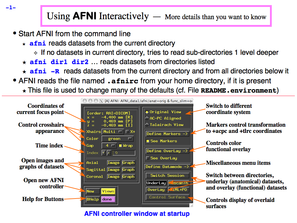
https://afni.nimh.nih.gov/pub/dist/doc/program_help/images/afni03/Slide01.png
------------------------------------------------------------------------------------
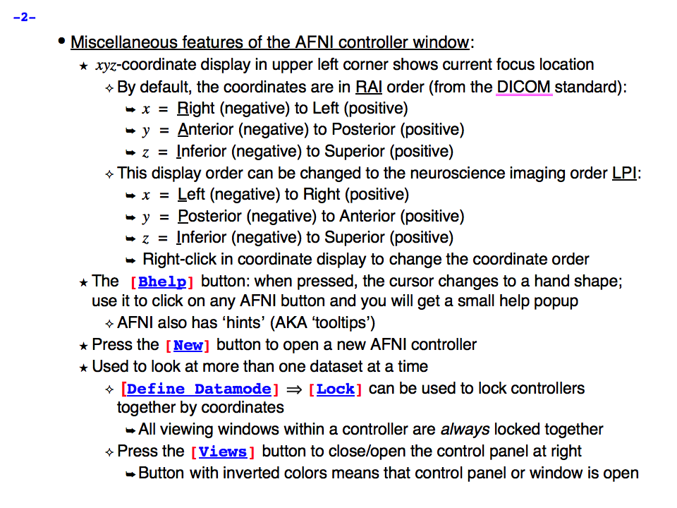
https://afni.nimh.nih.gov/pub/dist/doc/program_help/images/afni03/Slide02.png
------------------------------------------------------------------------------------
https://afni.nimh.nih.gov/pub/dist/doc/program_help/images/afni03/Slide03.png
------------------------------------------------------------------------------------
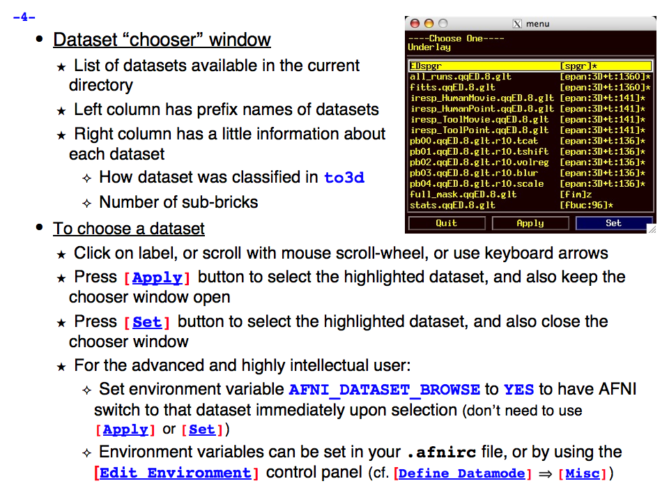
https://afni.nimh.nih.gov/pub/dist/doc/program_help/images/afni03/Slide04.png
------------------------------------------------------------------------------------
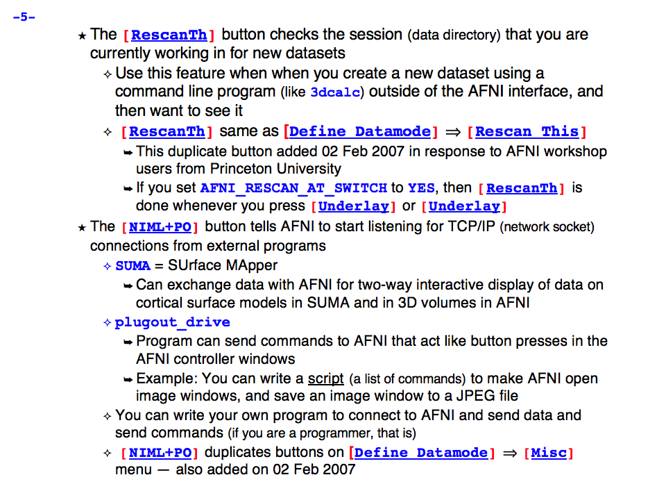
https://afni.nimh.nih.gov/pub/dist/doc/program_help/images/afni03/Slide05.png
------------------------------------------------------------------------------------

https://afni.nimh.nih.gov/pub/dist/doc/program_help/images/afni03/Slide06.png
------------------------------------------------------------------------------------
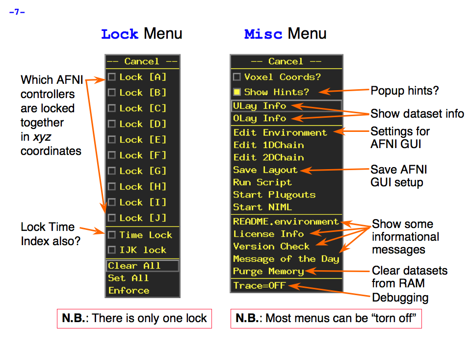
https://afni.nimh.nih.gov/pub/dist/doc/program_help/images/afni03/Slide07.png
------------------------------------------------------------------------------------
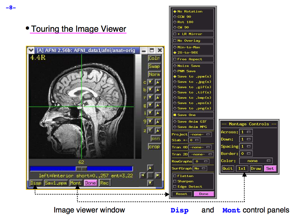
https://afni.nimh.nih.gov/pub/dist/doc/program_help/images/afni03/Slide08.png
------------------------------------------------------------------------------------
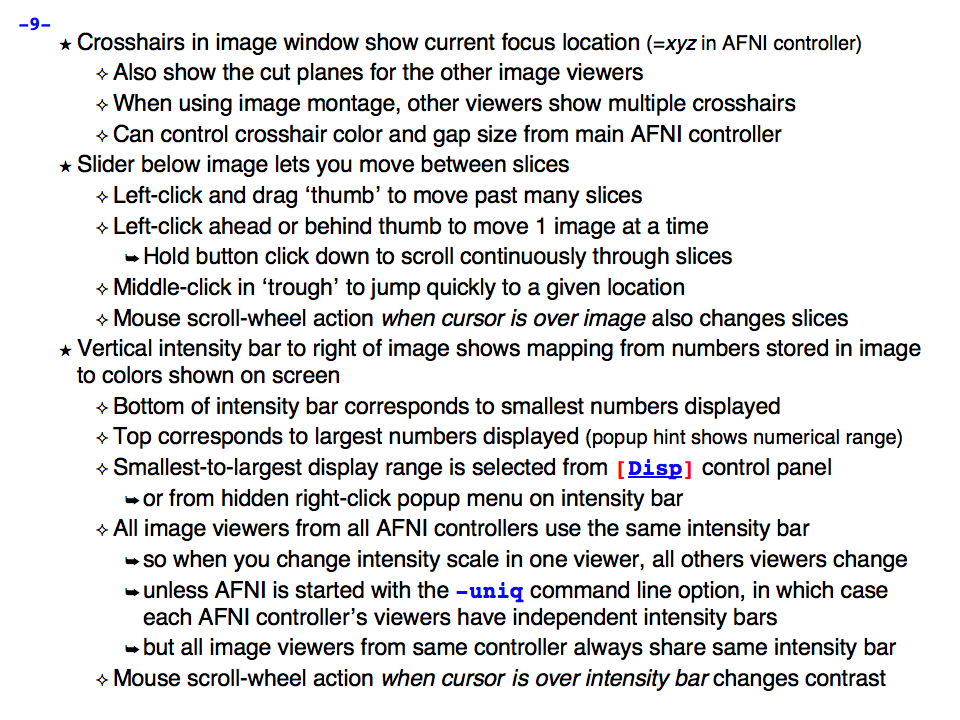
https://afni.nimh.nih.gov/pub/dist/doc/program_help/images/afni03/Slide09.png
------------------------------------------------------------------------------------
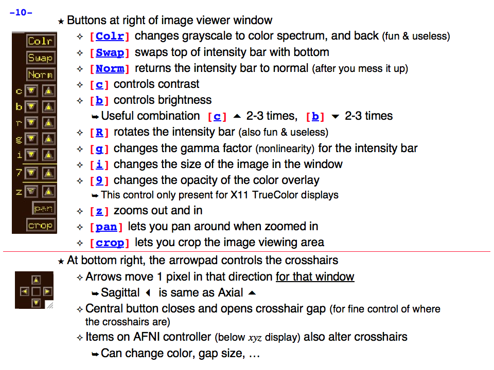
https://afni.nimh.nih.gov/pub/dist/doc/program_help/images/afni03/Slide10.png
------------------------------------------------------------------------------------
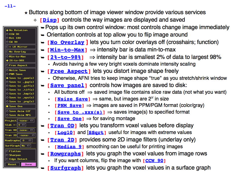
https://afni.nimh.nih.gov/pub/dist/doc/program_help/images/afni03/Slide11.png
------------------------------------------------------------------------------------
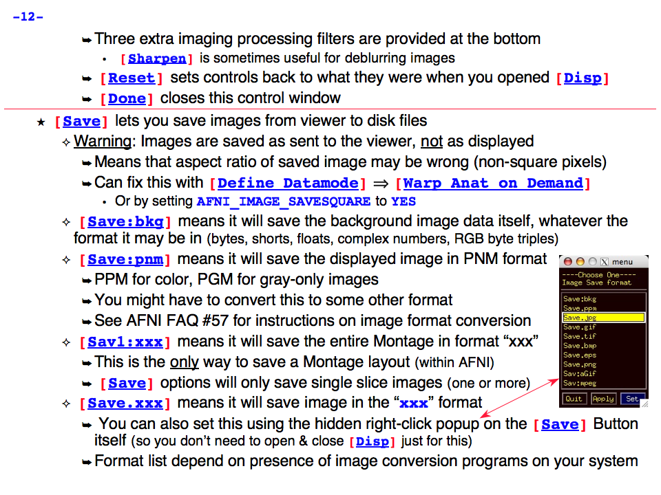
https://afni.nimh.nih.gov/pub/dist/doc/program_help/images/afni03/Slide12.png
------------------------------------------------------------------------------------
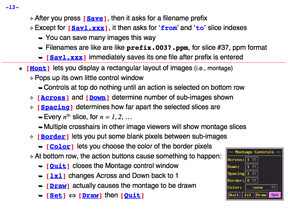
https://afni.nimh.nih.gov/pub/dist/doc/program_help/images/afni03/Slide13.png
------------------------------------------------------------------------------------

https://afni.nimh.nih.gov/pub/dist/doc/program_help/images/afni03/Slide14.png
------------------------------------------------------------------------------------
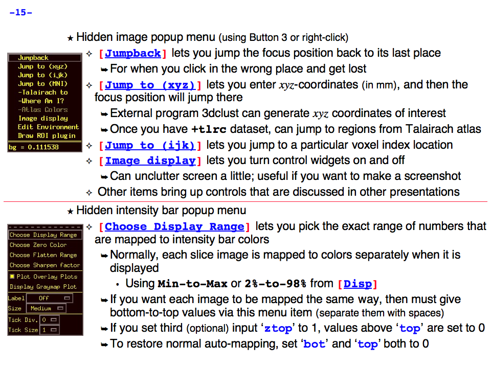
https://afni.nimh.nih.gov/pub/dist/doc/program_help/images/afni03/Slide15.png
------------------------------------------------------------------------------------
https://afni.nimh.nih.gov/pub/dist/doc/program_help/images/afni03/Slide16.png
------------------------------------------------------------------------------------

https://afni.nimh.nih.gov/pub/dist/doc/program_help/images/afni03/Slide17.png
------------------------------------------------------------------------------------
https://afni.nimh.nih.gov/pub/dist/doc/program_help/images/afni03/Slide18.png
------------------------------------------------------------------------------------
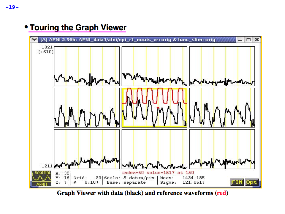
https://afni.nimh.nih.gov/pub/dist/doc/program_help/images/afni03/Slide19.png
------------------------------------------------------------------------------------
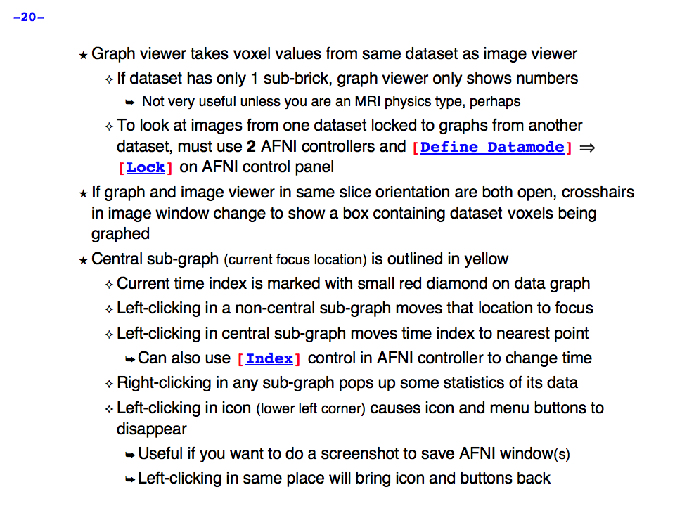
https://afni.nimh.nih.gov/pub/dist/doc/program_help/images/afni03/Slide20.png
------------------------------------------------------------------------------------

https://afni.nimh.nih.gov/pub/dist/doc/program_help/images/afni03/Slide21.png
------------------------------------------------------------------------------------
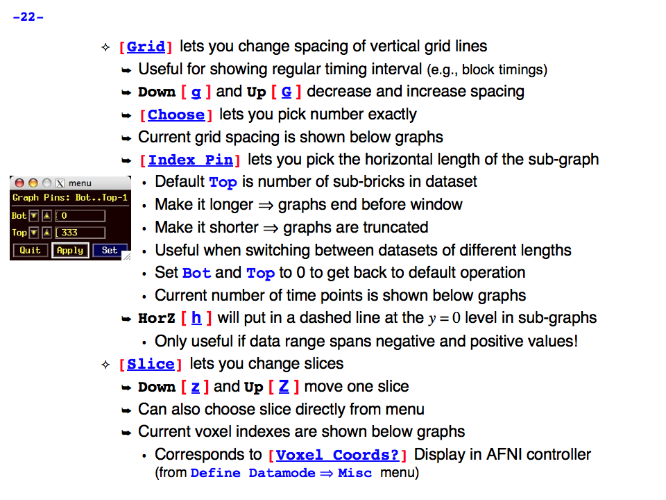
https://afni.nimh.nih.gov/pub/dist/doc/program_help/images/afni03/Slide22.png
------------------------------------------------------------------------------------
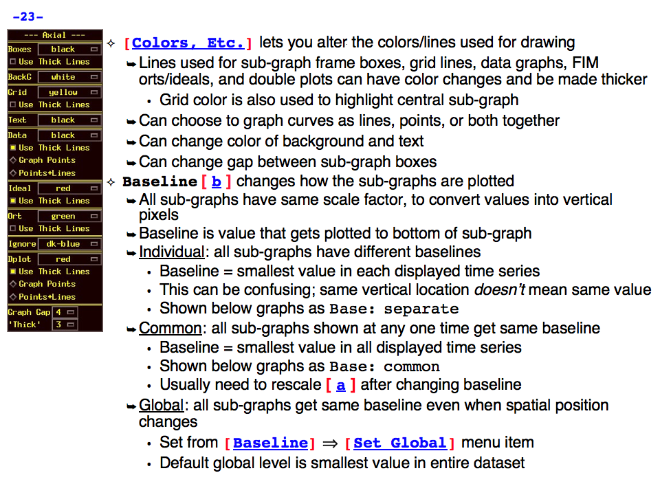
https://afni.nimh.nih.gov/pub/dist/doc/program_help/images/afni03/Slide23.png
------------------------------------------------------------------------------------
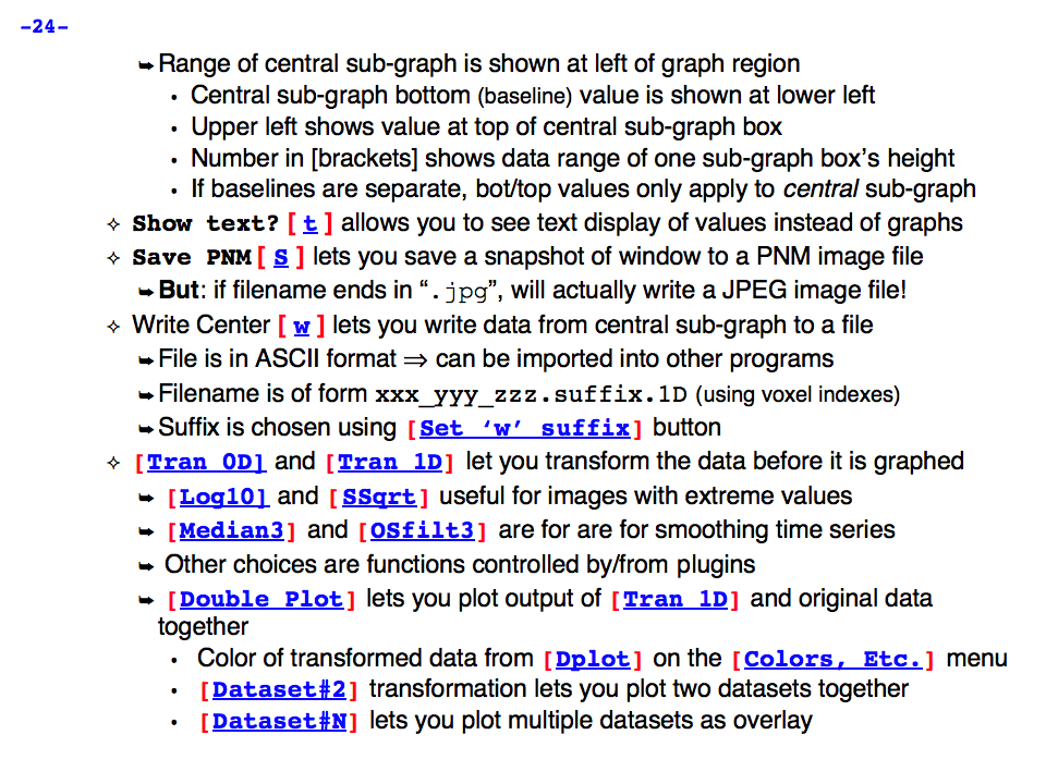
https://afni.nimh.nih.gov/pub/dist/doc/program_help/images/afni03/Slide24.png
------------------------------------------------------------------------------------
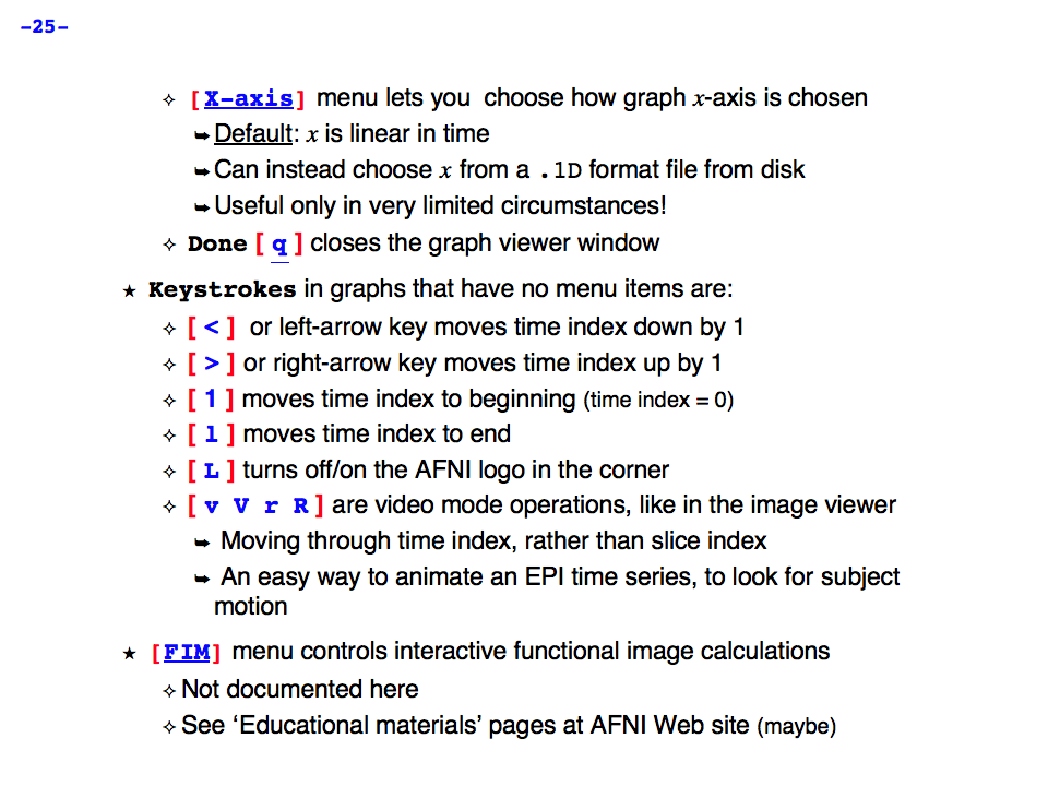
https://afni.nimh.nih.gov/pub/dist/doc/program_help/images/afni03/Slide25.png
------------------------------------------------------------------------------------
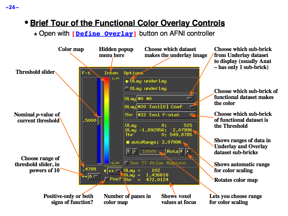
https://afni.nimh.nih.gov/pub/dist/doc/program_help/images/afni03/Slide26.png
------------------------------------------------------------------------------------

https://afni.nimh.nih.gov/pub/dist/doc/program_help/images/afni03/Slide27.png
------------------------------------------------------------------------------------
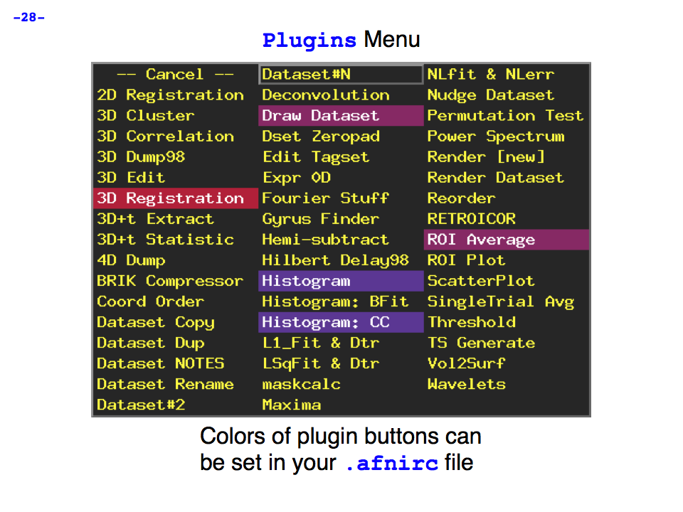
https://afni.nimh.nih.gov/pub/dist/doc/program_help/images/afni03/Slide28.png
------------------------------------------------------------------------------------
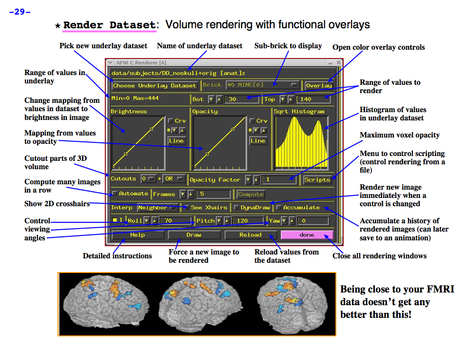
https://afni.nimh.nih.gov/pub/dist/doc/program_help/images/afni03/Slide29.png
------------------------------------------------------------------------------------
https://afni.nimh.nih.gov/pub/dist/doc/program_help/images/afni03/Slide30.png
------------------------------------------------------------------------------------
https://afni.nimh.nih.gov/pub/dist/doc/program_help/images/afni03/Slide31.png
------------------------------------------------------------------------------------
https://afni.nimh.nih.gov/pub/dist/doc/program_help/images/afni03/Slide32.png
------------------------------------------------------------------------------------
https://afni.nimh.nih.gov/pub/dist/doc/program_help/images/afni03/Slide33.png
------------------------------------------------------------------------------------
https://afni.nimh.nih.gov/pub/dist/doc/program_help/images/afni03/Slide34.png
------------------------------------------------------------------------------------
AFNI program: afni_check_omp
1
AFNI program: @AfniEnv
Script to set an AFNI environment variable in your afni resource file
Usage: @AfniEnv <-set NAME VALUE> [<-unset NAME>]
-set NAME VALUE: Set environment variable NAME to value VALUE
-get NAME: Get the value (same as apsearch -Vname option)
-unset NAME : The opposite of -set
-help: this message
Note that this script only modifies the contents of your .afnirc
file which is determined to be: /home/afniHQ/.afnirc
See also:
apsearch -afni_rc_file
apsearch -view_readme env
Global Help Options:
--------------------
-h_web: Open webpage with help for this program
-hweb: Same as -h_web
-h_view: Open -help output in a GUI editor
-hview: Same as -hview
-all_opts: List all of the options for this script
-h_find WORD: Search for lines containing WORD in -help
output. Seach is approximate.
AFNI program: afni_history
afni_history: show AFNI updates per user, dates or levels
This program is meant to display a log of updates to AFNI code, the
website, educational material, etc. Users can specify a level of
importance, the author, program or how recent the changes are.
The levels of importance go from 1 to 4, with meanings:
1 - users would not care
2 - of little importance, though some users might care
3 - fairly important
4 - a big change or new program
5 - IMPORTANT: we expect users to know
-----------------------------------------------------------------
common examples:
0. get help
a. afni_history -help
1. display all of the history, possibly subject to recent days/entries
a. afni_history
b. afni_history -past_days 5
c. afni_history -past_months 6
d. afni_history -past_entries 1
2. select a specific type, level or minimum level
a. afni_history -level 2
b. afni_history -min_level 3 -type BUG_FIX
c. afni_history -type 1 -min_level 3 -past_years 1
3. select a specific author or program
a. afni_history -author rickr
b. afni_history -program afni_proc.py
display the past year of updates for rickr, sorted by program name...
c. afni_history -author rickr -past_days 365 -final_sort_by_prog
4. select level 3+ suma updates from ziad over the past year
a. afni_history -author ziad -min_level 3 -program suma
5. generate a web-page, maybe from the past year at at a minimum level
a. afni_history -html -reverse > afni_hist_all.html
b. afni_history -html -reverse -min_level 2 > afni_hist_level2.html
c. afni_history -html -reverse -min_level 3 > afni_hist_level3.html
d. afni_history -html -reverse -min_level 4 > afni_hist_level4.html
5. verify that the distribution is new enough
Compare the most recent history entry against the passed date. If
there is a history entry as recent as the given date, it is current.
Otherwise, the distribution is considered old.
a. afni_history -check_date 1 1 2010
b. afni_history -check_date 15 Mar 2050
6. show particular fields
a. show the program name for the most recent 10 entries
afni_history -show_field program 10
b. show the program name for the most recent 10 NEW_PROG entries
afni_history -type NEW_PROG -show_field program 10
c. show the authors of the past 10 BUG_FIX entries
afni_history -type BUG_FIX -show_field author 10
d. show all unique program fields, sorted
afni_history -show_field program | sort | uniq
e. show all unique program fields of NEW_PROG entries, sorted
afni_history -show_field program -type NEW_PROG | sort | uniq
f. list FIELD parameters available for use with -show_field
afni_history -show_field_names
-----------------------------------------------------------------
------------------ informational options: -----------------------
-help : show this help
-hist : show this program's history
-list_authors : show the list of valid authors
-list_types : show the list of valid change types
-ver : show this program's version
------------------ output restriction options: ------------------
-author AUTHOR : restrict output to the given AUTHOR
-level LEVEL : restrict output to the given LEVEL
-min_level LEVEL : restrict output to at least level LEVEL
-program PROGRAM : restrict output to the given PROGRAM
-past_entries ENTRIES : restrict output to final ENTRIES entries
-past_days DAYS : restrict output to the past DAYS days
-past_months MONTHS : restrict output to the past MONTHS months
-past_years YEARS : restrict output to the past YEARS years
-type TYPE : restrict output to the given TYPE
(TYPE = 0..5, or strings 'NEW_PROG', etc.)
e.g. -type NEW_ENV
e.g. -type BUG_FIX
------------------ verification options: ------------------------
-check_date DD MM YYYY : check history against given date
If most recent afni_history is older than the passed date, the
distribution version might be considered out of date. Otherwise, it
might be considered current.
If the version seems okay, afni_history returns 0, else 1.
That way a script can check the status.
------------------ general options: -----------------------------
-html : add html formatting
-dline : put a divider line between dates
-reverse : reverse the sorting order
(sort is by date, author, level, program)
-show_field FIELD : restrict entry output to field FIELD
For each history entry printed in the output restrict the output
to only that implied by FIELD.
Valid FIELDs include:
FIELD : what to show
---------- ----------------------------------------
all : all fields (same as without -show_field)
firstline : only the standard first line
day : day of month
month : month of year
year : year of calendar system
date : year, month, day
author : author
program : program
level : level
type : type
desc : description
verbtext : verbtext
Only one -field option is allowed at the moment.
Valid FIELD values can be shown by
afni_history -show_field_names
-show_field_names : list valid FIELD names for -show_field
Each entry in the output list can be passed to -show_field
-verb LEVEL : request verbose output
(LEVEL is from 0-6)
Author: Rick Reynolds
Thanks to: Ziad, Bob
AFNI program: afni_open
A program to open various AFNI/SUMA files
afni_open [OPTIONS] FILE1 [FILE2 ...]
Examples:
afni_open xmat.1D.xmat
afni_open -aw roi_11.pdf
afni_open -r driv
Options:
===========
-w METHOD: Use METHOD to open FILES.
Acceptable values for METHOD are:
editor :Open with text editor.
downloader :Fetch with wget or curl.
browser :Open in browser
afni :Open with AFNI
suma :Open with SUMA
1dplot :Open with 1dplot
ExamineXmat :Open with ExamineXmat
iviewer :Open with image viewer
spreadsheet :Open with spreadsheet viewer
afniweb :Get from afni website.
readme :Search for appropriate README
This option is in the same spirit of
apsearch -view_readme option. To see a list of
all readme files, run:
apsearch -list_all_afni_readmes
-e :Same as -w editor
-d :Same as -w downloader
-x :Same as -w ExamineXmat
-b :Same as -w browser
-r :Same as -w readme
-s :Same as -w spreadsheet
-aw :Same as -w afniweb
NB: If no method is specified, the program tries to guess
from the filename.
-global_help :Show help for global options.
-gopts_help :Show help for global options.
-help :You're looking at it.
Global Options:
===============
-h: Mini help, at time, same as -help in many cases.
-help: The entire help output
-HELP: Extreme help, same as -help in majority of cases.
-h_view: Open help in text editor. AFNI will try to find a GUI editor
-hview : on your machine. You can control which it should use by
setting environment variable AFNI_GUI_EDITOR.
-h_web: Open help in web browser. AFNI will try to find a browser.
-hweb : on your machine. You can control which it should use by
setting environment variable AFNI_GUI_EDITOR.
-h_find WORD: Look for lines in this programs's -help output that match
(approximately) WORD.
-h_raw: Help string unedited
-h_spx: Help string in sphinx loveliness, but do not try to autoformat
-h_aspx: Help string in sphinx with autoformatting of options, etc.
-all_opts: Try to identify all options for the program from the
output of its -help option. Some options might be missed
and others misidentified. Use this output for hints only.
-overwrite: Overwrite existing output dataset.
Equivalent to setting env. AFNI_DECONFLICT=OVERWRITE
-ok_1D_text: Zero out uncommented text in 1D file.
Equivalent to setting env. AFNI_1D_ZERO_TEXT=YES
-Dname=val: Set environment variable 'name' to value 'val'
For example: -DAFNI_1D_ZERO_TEXT=YES
-Vname=: Print value of environment variable 'name' to stdout and quit.
This is more reliable that the shell's env query because it would
include envs set in .afnirc files and .sumarc files for SUMA
programs.
For example: -VAFNI_1D_ZERO_TEXT=
-skip_afnirc: Do not read the afni resource (like ~/.afnirc) file.
-pad_to_node NODE: Output a full dset from node 0 to MAX_NODE-1
** Instead of directly setting NODE to an integer you
can set NODE to something like:
ld120 (or rd17) which sets NODE to be the maximum
node index on an Icosahedron with -ld 120. See
CreateIcosahedron for details.
d:DSET.niml.dset which sets NODE to the maximum node found
in dataset DSET.niml.dset.
** This option is for surface-based datasets only.
Some programs may not heed it, so check the output if
you are not sure.
-pif SOMETHING: Does absolutely nothing but provide for a convenient
way to tag a process and find it in the output of ps -a
-echo_edu: Echos the entire command line to stdout (without -echo_edu)
for edification purposes
SPECIAL PURPOSE ARGUMENTS TO ADD *MORE* ARGUMENTS TO THE COMMAND LINE
------------------------------------------------------------------------
Arguments of the following form can be used to create MORE command
line arguments -- the principal reason for using these type of arguments
is to create program command lines that are beyond the limit of
practicable scripting. (For one thing, Unix command lines have an
upper limit on their length.) This type of expanding argument makes
it possible to input thousands of files into an AFNI program command line.
The generic form of these arguments is (quotes, 'single' or "double",
are required for this type of argument):
'<<XY list'
where X = I for Include (include strings from file)
or X = G for Glob (wildcard expansion)
where Y = M for Multi-string (create multiple arguments from multiple strings)
or Y = 1 for One-string (all strings created are put into one argument)
Following the XY modifiers, a list of strings is given, separated by spaces.
* For X=I, each string in the list is a filename to be read in and
included on the command line.
* For X=G, each string in the list is a Unix style filename wildcard
expression to be expanded and the resulting filenames included
on the command line.
In each case, the '<<XY list' command line argument will be removed and
replaced by the results of the expansion.
* '<<GM wildcards'
Each wildcard string will be 'globbed' -- expanded from the names of
files -- and the list of files found this way will be stored in a
sequence of new arguments that replace this argument:
'<<GM ~/Alice/*.nii ~/Bob/*.nii'
might expand into a list of hundreds of separate datasets.
* Why use this instead of just putting the wildcards on the command
line? Mostly to get around limits on the length of Unix command lines.
* '<<G1 wildcards'
The difference from the above case is that after the wildcard expansion
strings are found, they are catenated with separating spaces into one
big string. The only use for this in AFNI is for auto-catenation of
multiple datasets into one big dataset.
* '<<IM filenames'
Each filename string will result in the contents of that text file being
read in, broken at whitespace into separate strings, and the resulting
collection of strings will be stored in a sequence of new arguments
that replace this argument. This type of argument can be used to input
large numbers of files which are listed in an external file:
'<<IM Bob.list.txt'
which could in principle result in reading in thousands of datasets
(if you've got the RAM).
* This type of argument is in essence an internal form of doing something
like `cat filename` using the back-quote shell operator on the command
line. The only reason this argument (or the others) was implemented is
to get around the length limits on the Unix command line.
* '<<I1 filenames'
The difference from the above case is that after the files are read
and their strings are found, they are catenated with separating spaces
into one big string. The only use for this in AFNI is for auto-catenation
of multiple datasets into one big dataset.
* 'G', 'M', and 'I' can be lower case, as in '<<gm'.
* 'glob' is Unix jargon for wildcard expansion:
https://en.wikipedia.org/wiki/Glob_(programming)
* If you set environment variable AFNI_GLOB_SELECTORS to YES,
then the wildcard expansion with '<<g' will not use the '[...]'
construction as a Unix wildcard. Instead, it will expand the rest
of the wildcard and then append the '[...]' to the results:
'<<gm fred/*.nii[1..100]'
would expand to something like
fred/A.nii[1..100] fred/B.nii[1..100] fred/C.nii[1..100]
This technique is a way to preserve AFNI-style sub-brick selectors
and have them apply to a lot of files at once.
Another example:
3dttest++ -DAFNI_GLOB_SELECTORS=YES -brickwise -prefix Junk.nii \
-setA '<<gm sub-*/func/*rest_bold.nii.gz[0..100]'
* However, if you want to put sub-brick selectors on the '<<im' type
of input, you will have to do that in the input text file itself
(for each input filename in that file).
* BE CAREFUL OUT THERE!
------------------------------------------------------------------------
++ Compile date = Jul 6 2026 {AFNI_26.2.01:linux_ubuntu_24_64}
AFNI program: @AfniOrient2RAImap
Usage: @AfniOrient2RAImap <Orientation code> .....
returns the index map fo the RAI directions
examples:
@AfniOrient2RAImap RAI
returns: 1 2 3
@AfniOrient2RAImap LSP
returns: -1 -3 -2
Ziad Saad (saadz@mail.nih.gov)
SSCC/NIMH/ National Institutes of Health, Bethesda Maryland
AFNI program: afni_proc.py
===========================================================================
afni_proc.py - generate a tcsh script for an AFNI process stream
Purpose: ~1~
This program is meant to create single subject processing scripts for
task, resting state or surface-based analyses. The processing scripts
are written in the tcsh language.
The typical goal is to create volumes of aligned response magnitudes
(stimulus beta weights) to use as input for a group analysis.
Inputs (only EPI is required): ~1~
- anatomical dataset
- EPI time series datasets
- stimulus timing files
- processing and design decisions:
e.g. TRs to delete, blur size, censoring options, basis functions
Main outputs (many datasets are created): ~1~
- for task-based analysis: stats dataset (and anat_final)
- for resting-state analysis: errts datasets ("cleaned up" EPI)
Basic script outline: ~1~
- copy all inputs to new 'results' directory
- process data: e.g. despike,tshift/align/tlrc/volreg/blur/scale/regress
- leave all (well, most) results there, so user can review processing
- create quality control data (APQC HTML page, ss_review_scripts, etc.)
The exact processing steps are controlled by the user, including which main
processing blocks to use, and their order. See the 'DEFAULTS' section for
a description of the default options for each block.
The output script (when executed) would create a results directory, copy
input files into it, and perform all processing there. So the user can
delete the results directory and modify/re-run the script at their whim.
Note that the user need not actually run the output script. The user
should feel free to modify the script for their own evil purposes, or to
just compare the processing steps with those in their own scripts. Also,
even if a user is writing their own processing scripts, it is a good idea
to get some independent confirmation of the processing, such as by using
afni_proc.py to compare the results on occasion.
The text interface can be accessed via the -ask_me option. It invokes a
question & answer session, during which this program sets user options on
the fly. The user may elect to enter some of the options on the command
line, even if using -ask_me. See "-ask_me EXAMPLES", below.
** However, -ask_me has not been touched in many years. I suggest starting
with the 'modern' examples (for task/rest/surface), or by using the
uber_subject.py GUI (graphical user interface) to generate an initial
afni_proc.py command script.
See uber_subject.py -help (or just start the GUI) for details.
==================================================
SECTIONS: order of sections in the "afni_proc.py -help" output ~1~
program introduction : (above) basic overview of afni_proc.py
SETTING UP AN ANALYSIS : a guide for getting started
PROCESSING BLOCKS : list of possible processing blocks
DEFAULTS : basic default operations, per block
EXAMPLES : various examples of running this program
NOTE sections : details on various topics
GENERAL ANALYSIS NOTE, QUALITY CONTROL NOTE,
RESTING STATE NOTE, FREESURFER NOTE,
TIMING FILE NOTE, MASKING NOTE,
ANAT/EPI ALIGNMENT CASES NOTE, ANAT/EPI ALIGNMENT CORRECTIONS NOTE,
WARP TO TLRC NOTE,
RETROICOR NOTE, MULTI ECHO NOTE,
RUNS OF DIFFERENT LENGTHS NOTE, SCRIPT EXECUTION NOTE
OPTIONS : descriptions of all program options
informational : options to get quick info and quit
general execution : options not specific to a processing block
block options : specific to blocks, in default block order
==================================================
SETTING UP AN ANALYSIS: ~1~
For those new to using afni_proc.py, it is very helpful to start with an
example that is similar to what you want to do, generally taken from the help
examples (afni_proc.py -show_example_names) or prior publication.
Once satisfied with a single application of afni_proc.py, one would then loop
over subjects by running afni_proc.py on each, using subject variables to refer
to the individual set of input data and the output subject ID.
Starting up, there is a general set of choices that is good to consider:
a. type of analysis: task or rest/naturalistic
b. domain of analysis: volume or surface (possibly either as ROI)
c. main input data: anat, EPI runs (single or multi-echo), task timing,
surfaces and surface anatomical
d. extra input data: NL distortion warp, NL template warp, blip dsets,
ROI imports, anat followers, physio regressors,
external registration base (for volreg or anat),
external motion files, censor list, extra regressors
e. processing blocks: main EPI processing blocks and their order
- see "PROCESSING BLOCKS"
f. optional processing: physio regression, tedana, ANATICOR, ROI regression,
bandpassing
g. main options: template, blur level (if any), censor levels,
EPI/anat cost and other alignment options
h. other options: there are many, e.g.: motion regressors, bandpass,
ANATICOR, and many that are specific to QC
----------
a. type of analysis
For a task analysis, one provides stimulus timing files and corresponding
modeling options. This is a large topic that centers on the use of
3dDeconvolve.
Options for task analysis generally start with -regress, as they pertain
to the regress block. However one generally includes a regress block in
any analysis (even partial ones, such as for alignment), as it is the
gateway to the APQC HTML report.
b. domain of analysis
For a surface analysis, one provides a SUMA spec file per hemisphere,
along with a surface anatomical dataset. Mapping from the volume to the
surface generally happens soon after all volumetric registration is done,
and importantly, before any blur block. Restricting blurring to the
surface is one of the reasons to perform such an analysis.
In a surface analysis, no volumetric template or tlrc options are given.
Surface analysis is generally performed on SUMA's standard meshes, though
it need not be.
An ROI analysis is generally performed as a typical volume or surface
analysis, but without any applied blurring (which effectively happens
later, when averaging over the ROIs).
c. main input data
EPI datasets are required, for one or more runs and one or more echoes.
Anything else is optional.
Typically one also includes a subject anatomy, any task timing files, and
surface datasets (spec files an anatomy) if doing a surface analysis.
d. extra input data
It is common to supply a non-linear transformation warp dataset (from
sswarper) to apply for anatomy->template alignment. One might also have
a pre-computed non-linear B0 distortion map or reverse phase encoding
(blip) dataset, ROIs or other anatomical followers or physiological
regressors. An EPI base dataset might be provided to align the EPI to,
and possibly one to guide alignment to the subject anatomical dataset.
Precomputed motion parameter files could be provided (if skipping the
volreg block), as well as an external censor time series or precomputed
regressors (of interest or not).
These extra inputs will affect use of other options.
e. processing blocks
As described in the "PROCESSING BLOCKS" section, one can specify an
ordered list of main processing blocks. The order of the listed blocks
will determine their order in the processing script. Of course, for a
given set of blocks, there is typically a preferred order.
Options specific to one block will generally start with that block name.
For example, the -regress_* options apply to the regress block.
It is logically clear (but not necessary) to provide block options in the
same chronological order as the blocks.
f. optional processing
Optional processing might include things like:
- physiological noise regression, based on use of physio_calc.py
- tedana, or a variant, for use in combining multi-echo time series
- ANATICOR (local white matter regression)
- ROI regression (averages or principle components)
- bandpassing (low pass, high pass, or single or multiple bands)
g. main options
One typically provides:
- a template (and accompanying non-linear anat to template
transformation datasets)
- an amount to blur (or a choice to not blur, as would apply to an ROI
analysis), or a level to blur _to_
- censor levels (for outliers or the Euclidean norm of the motion
parameters)
- alignment options, such as the cost function for align_epi_anat.py
and a local EPI unifize option - there are many options to control
many aspects of registration
- many quality control options are also considered appropriate for
consistent use
h. other options
Each step of processing has many control options around it. It is
important to think through what might be appropriate for the data in
question.
No one analysis fits all data.
Quality control "options" are not really considered optional.
==================================================
PROCESSING BLOCKS (of the output script): ~1~
The output script will go through the following steps, unless the user
specifies otherwise.
automatic blocks (the tcsh script will always perform these): ~2~
setup : check subject arg, set run list, create output dir, and
copy stim files
tcat : copy input datasets and remove unwanted initial TRs
default blocks (the user may skip these, or alter their order): ~2~
tshift : slice timing alignment on volumes (default is -time 0)
volreg : volume registration (default to third volume)
blur : blur each volume (default is 4mm fwhm)
mask : create a 'brain' mask from the EPI data
scale : scale each run mean to 100, for each voxel (max of 200)
regress : regression analysis (default is GAM, peak 1, with motion
params)
optional blocks (the default is to _not_ apply these blocks) ~2~
align : align EPI anat anatomy (via align_epi_anat.py)
combine : combine echoes into one
despike : truncate spikes in each voxel's time series
empty : placeholder for some user command (uses 3dTcat as sample)
ricor : RETROICOR - removal of cardiac/respiratory regressors
surf : project volumetric data into the surface domain
tlrc : warp anat to a standard space/specified template
implicit blocks (controlled by program, added when appropriate) ~2~
blip : perform B0 distortion correction
outcount : temporal outlier detection
QC review : generate QC review scripts and HTML report
anat_unif : anatomical uniformity correction
==================================================
DEFAULTS: basic defaults for each block (blocks listed in default order) ~1~
A : denotes automatic block that is not a 'processing' option
D : denotes a default processing block (others must be requested)
A setup: - use 'SUBJ' for the subject id
(option: -subj_id SUBJ)
- create a t-shell script called 'proc_subj'
(option: -script proc_subj)
- use results directory 'SUBJ.results'
(option: -out_dir SUBJ.results)
A tcat: - do not remove any of the first TRs
despike: - NOTE: by default, this block is _not_ used
- automasking is not done (requires -despike_mask)
ricor: - NOTE: by default, this block is _not_ used
- polort based on twice the actual run length
- solver is OLSQ, not REML
- do not remove any first TRs from the regressors
D tshift: - align slices to the beginning of the TR
- use quintic interpolation for time series resampling
(option: -tshift_interp -quintic)
align: - align the anatomy to match the EPI
(also required for the option of aligning EPI to anat)
tlrc: - use TT_N27+tlrc as the base (-tlrc_base TT_N27+tlrc)
- no additional suffix (-tlrc_suffix NONE)
- use affine registration (no -tlrc_NL_warp)
D volreg: - align to third volume of first run, -zpad 1
(option: -volreg_align_to third)
(option: -volreg_zpad 1)
- use cubic interpolation for volume resampling
(option: -volreg_interp -cubic)
- apply motion params as regressors across all runs at once
- do not align EPI to anat
- do not warp to standard space
combine: - combine methods using OC (optimally combined)
D blur: - blur data using a 4 mm FWHM filter with 3dmerge
(option: -blur_filter -1blur_fwhm)
(option: -blur_size 4)
(option: -blur_in_mask no)
D mask: - create a union of masks from 3dAutomask on each run
- not applied in regression without -regress_apply_mask
- if possible, create a subject anatomy mask
- if possible, create a group anatomy mask (tlrc base)
D scale: - scale each voxel to mean of 100, clip values at 200
D regress: - use GAM regressor for each stim
(option: -regress_basis)
- compute the baseline polynomial degree, based on run length
(e.g. option: -regress_polort 2)
- do not censor large motion
- output fit time series
- output ideal curves for GAM/BLOCK regressors
- output iresp curves for non-GAM/non-BLOCK regressors
empty: - do nothing (just copy the data using 3dTcat)
==================================================
EXAMPLES (options can be provided in any order): ~1~
Example 1. Minimum use. ~2~
(recommended? no, not intended for a complete analysis)
( merely shows how simple a command can be)
Provide datasets and stim files (or stim_times files). Note that a
dataset suffix (e.g. HEAD) must be used with wildcards, so that
datasets are not applied twice. In this case, a stim_file with many
columns is given, where the script to changes it to stim_times files.
--------------------------
last mod date : 2008.12.10
keywords : obsolete, task
--------------------------
afni_proc.py \
-dsets epiRT*.HEAD \
-regress_stim_files stims.1D
Example 2. Very simple. ~2~
(recommended? no, not intended for a complete analysis)
( many missing preferences, e.g. @SSwarper)
Use all defaults, except remove 3 TRs and use basis
function BLOCK(30,1). The default basis function is GAM.
--------------------------
last mod date : 2009.05.28
keywords : obsolete, task
--------------------------
afni_proc.py \
-subj_id sb23.e2.simple \
-dsets sb23/epi_r??+orig.HEAD \
-tcat_remove_first_trs 3 \
-regress_stim_times sb23/stim_files/blk_times.*.1D \
-regress_basis 'BLOCK(30,1)'
Example 3. Formerly a simple class example. ~2~
(recommended? no, not intended for a complete analysis)
( many missing preferences, e.g. @SSwarper)
Copy the anatomy into the results directory, register EPI data to
the last TR, specify stimulus labels, compute blur estimates, and
provide GLT options directly to 3dDeconvolve. The GLTs will be
ignored after this, as they take up too many lines.
--------------------------
last mod date : 2009.05.28
keywords : obsolete, task
--------------------------
afni_proc.py \
-subj_id sb23.blk \
-dsets sb23/epi_r??+orig.HEAD \
-copy_anat sb23/sb23_mpra+orig \
-tcat_remove_first_trs 3 \
-volreg_align_to last \
-regress_stim_times sb23/stim_files/blk_times.*.1D \
-regress_stim_labels tneg tpos tneu eneg epos eneu fneg fpos \
fneu \
-regress_basis 'BLOCK(30,1)' \
-regress_opts_3dD -gltsym 'SYM: +eneg -fneg' \
-glt_label 1 eneg_vs_fneg \
-gltsym \
'SYM: 0.5*fneg 0.5*fpos -1.0*fneu' \
-glt_label 2 face_contrast \
-gltsym \
'SYM: tpos epos fpos -tneg -eneg -fneg' \
-glt_label 3 pos_vs_neg \
-regress_est_blur_epits \
-regress_est_blur_errts
Example 4. Similar to 3, but specify the processing blocks. ~2~
(recommended? no, not intended for a complete analysis)
( many missing preferences, e.g. @SSwarper)
Adding despike and tlrc, and removing tshift. Note that
the tlrc block is to run @auto_tlrc on the anat. Ignore the GLTs.
--------------------------
last mod date : 2009.05.28
keywords : obsolete, task
--------------------------
afni_proc.py \
-subj_id sb23.e4.blocks \
-dsets sb23/epi_r??+orig.HEAD \
-blocks despike volreg blur mask scale regress \
tlrc \
-copy_anat sb23/sb23_mpra+orig \
-tcat_remove_first_trs 3 \
-regress_stim_times sb23/stim_files/blk_times.*.1D \
-regress_stim_labels tneg tpos tneu eneg epos eneu fneg fpos \
fneu \
-regress_basis 'BLOCK(30,1)' \
-regress_est_blur_epits \
-regress_est_blur_errts
Example 5a. RETROICOR, resting state data. ~2~
(recommended? no, not intended for a complete analysis)
( just a terribly simple example using ricor)
Assuming the class data is for resting-state and that we have the
appropriate slice-based regressors from RetroTS.py, apply the
despike and ricor processing blocks. Note that '-do_block' is used
to add non-default blocks into their default positions. Here the
'despike' and 'ricor' processing blocks would come before 'tshift'.
Remove 3 TRs from the ricor regressors to match the EPI data. Also,
since degrees of freedom are not such a worry, regress the motion
parameters per-run (each run gets a separate set of 6 regressors).
The regression will use 81 basic regressors (all of "no interest"),
with 13 retroicor regressors being removed during preprocessing:
27 baseline regressors ( 3 per run * 9 runs)
54 motion regressors ( 6 per run * 9 runs)
To example #3, add -do_block, -ricor_* and -regress_motion_per_run.
--------------------------
last mod date : 2009.05.28
keywords : obsolete, physio, rest
--------------------------
afni_proc.py \
-subj_id sb23.e5a.ricor \
-dsets sb23/epi_r??+orig.HEAD \
-do_block despike ricor \
-tcat_remove_first_trs 3 \
-ricor_regs_nfirst 3 \
-ricor_regs sb23/RICOR/r*.slibase.1D \
-regress_motion_per_run
If tshift, blurring and masking are not desired, consider replacing
the -do_block option with an explicit list of blocks:
-blocks despike ricor volreg regress
Example 5b. RETROICOR, while running a normal regression. ~2~
(recommended? no, not intended for a complete analysis)
( another overly simple example using ricor)
Add the ricor regressors to a normal regression-based processing
stream. Apply the RETROICOR regressors across runs (so using 13
concatenated regressors, not 13*9). Note that concatenation is
normally done with the motion regressors too.
To example #3, add -do_block and three -ricor options.
--------------------------
last mod date : 2009.05.28
keywords : obsolete, physio, rest
--------------------------
afni_proc.py \
-subj_id sb23.e5b.ricor \
-dsets sb23/epi_r??+orig.HEAD \
-do_block despike ricor \
-copy_anat sb23/sb23_mpra+orig \
-tcat_remove_first_trs 3 \
-ricor_regs_nfirst 3 \
-ricor_regs sb23/RICOR/r*.slibase.1D \
-ricor_regress_method across-runs \
-volreg_align_to last \
-regress_stim_times sb23/stim_files/blk_times.*.1D \
-regress_stim_labels tneg tpos tneu eneg epos eneu fneg fpos \
fneu \
-regress_basis 'BLOCK(30,1)' \
-regress_est_blur_epits \
-regress_est_blur_errts
Also consider adding -regress_bandpass.
Example 5c. RETROICOR: censor and band pass. ~2~
(recommended? no, not intended for a complete analysis)
( many missing preferences, e.g. @SSwarper, no BP)
This is an example of how we might currently suggest analyzing
resting state data. If no RICOR regressors exist, see example 9
(or just remove any ricor options).
Censoring due to motion has long been considered appropriate in
BOLD FMRI analysis, but is less common for those doing bandpass
filtering in RS FMRI because the FFT requires one to either break
the time axis (evil) or to replace the censored data with something
probably inappropriate.
Instead, it is slow (no FFT, but maybe SFT :) but effective to
regress frequencies within the regression model, where censoring
is simple.
Note: band passing in the face of RETROICOR is questionable. It may
be questionable in general. To skip bandpassing, remove the
-regress_bandpass option line.
Also, align EPI to anat and warp to standard space.
--------------------------
last mod date : 2016.05.03
keywords : obsolete, physio, task
--------------------------
afni_proc.py \
-subj_id sb23.e5a.ricor \
-dsets sb23/epi_r??+orig.HEAD \
-blocks despike ricor tshift align tlrc volreg \
blur mask regress \
-copy_anat sb23/sb23_mpra+orig \
-tcat_remove_first_trs 3 \
-ricor_regs_nfirst 3 \
-ricor_regs sb23/RICOR/r*.slibase.1D \
-volreg_align_e2a \
-volreg_tlrc_warp \
-blur_size 6 \
-regress_bandpass 0.01 0.1 \
-regress_apply_mot_types demean deriv \
-regress_motion_per_run \
-regress_censor_motion 0.2 \
-regress_run_clustsim no \
-regress_est_blur_epits \
-regress_est_blur_errts
Example 6. A simple task example, based on AFNI_data6. ~2~
(recommended? no, not intended for a complete analysis)
( meant to be fast, but not complete, e.g. NL warp)
( prefer: see Example 6b)
This example has changed to more closely correspond with the
the class analysis example, AFNI_data6/FT_analysis/s05.ap.uber.
The tshift block will interpolate each voxel time series to adjust
for differing slice times, where the result is more as if each
entire volume were acquired at the beginning of the TR.
The 'align' block implies using align_epi_anat.py to align the
anatomy with the EPI. Here, the EPI base is first unifized locally.
Additional epi/anat alignment options specify using lpc+ZZ for the
cost function (more robust than simply lpc), -giant_move (in case
the anat and EPI start a bit far apart), and -check_flip, to try to
verify whether EPI left and right agree with the anatomy.
This block computes the anat to EPI transformation matrix, which
will be inverted in the volreg block, based on -volreg_align_e2a.
Also, compute the transformation of the anatomy to MNI space, using
affine registration (for speed in this simple example) to align to
the 2009c template.
In the volreg block, align the EPI to the MIN_OUTLIER volume (a
low-motion volume, determined based on the data). Then concatenate
all EPI transformations, warping the EPI to standard space in one
step (without multiple resampling operations), combining:
EPI -> EPI base -> anat -> MNI 2009c template
The standard space transformation is included by specifying option
-volreg_tlrc_warp.
A 4 mm blur is applied, to keep it very light (about 1.5 times the
voxel size).
The regression model is based on 2 conditions, each lasting 20 s
per event, modeled by convolving a 20 s boxcar function with the
BLOCK basis function, specified as BLOCK(20,1) to make the regressor
unit height (height 1).
One extra general linear test (GLT) is included, contrasting the
visual reliable condition (vis) with auditory reliable (aud).
Motion regression will be per run (using one set of 6 regressors for
each run, i.e. 18 regressors in this example).
The regression includes censoring of large motion (>= 0.3 ~mm
between successive time points, based on the motion parameters),
as well as censoring of outlier time points, where at least 5% of
the brain voxels are computed as outliers.
The regression model starts as a full time series, for time
continuity, before censored time points are removed. The output
errts will be zero at censored time points (no error there), and so
the output fit times series (fitts) will match the original data.
The model fit time series (fitts) will be computed AFTER the linear
regression, to save RAM on class laptops.
Create sum_ideal.1D, as the sum of all non-baseline regressors, for
quality control.
Estimate the blur in the residual time series. The resulting 3 ACF
parameters can be averaged across subjects for cluster correction at
the group level.
Skip running the Monte Carlo cluster simulation example (which would
specify minimum cluster sizes for cluster significance, based on the
ACF parameters and mask), for speed.
Once the proc script is created, execute it.
--------------------------
last mod date : 2020.02.15
keywords : task
--------------------------
afni_proc.py \
-subj_id FT.e6 \
-copy_anat FT/FT_anat+orig \
-dsets FT/FT_epi_r?+orig.HEAD \
-blocks tshift align tlrc volreg mask blur \
scale regress \
-radial_correlate_blocks tcat volreg \
-tcat_remove_first_trs 2 \
-align_unifize_epi local \
-align_opts_aea -cost lpc+ZZ \
-giant_move \
-check_flip \
-tlrc_base MNI152_2009_template.nii.gz \
-volreg_align_to MIN_OUTLIER \
-volreg_align_e2a \
-volreg_tlrc_warp \
-volreg_compute_tsnr yes \
-mask_epi_anat yes \
-blur_size 4.0 \
-regress_stim_times FT/AV1_vis.txt FT/AV2_aud.txt \
-regress_stim_labels vis aud \
-regress_basis 'BLOCK(20,1)' \
-regress_opts_3dD -jobs 2 \
-gltsym 'SYM: vis -aud' \
-glt_label 1 V-A \
-regress_motion_per_run \
-regress_censor_motion 0.3 \
-regress_censor_outliers 0.05 \
-regress_compute_fitts \
-regress_make_ideal_sum sum_ideal.1D \
-regress_est_blur_epits \
-regress_est_blur_errts \
-regress_run_clustsim no \
-html_review_style pythonic \
-execute
* One could also use ANATICOR with task (e.g. -regress_anaticor_fast)
in the case of -regress_reml_exec. 3dREMLfit supports voxelwise
regression, but 3dDeconvolve does not.
Example 6b. A modern task example, with preferable options. ~2~
(recommended? yes, reasonable for a complete analysis)
GOOD TO CONSIDER
This is based on Example 6, but is more complete.
Example 6 is meant to run quickly, as in an AFNI bootcamp setting.
Example 6b is meant to process more as we might suggest.
- apply -check_flip in align_epi_anat.py, to monitor consistency
- apply non-linear registration to MNI template, using output
from @SSwarper:
o apply skull-stripped anat in -copy_anat
o apply original anat as -anat_follower (QC, for comparison)
o pass warped anat and transforms via -tlrc_NL_warped_dsets,
to apply those already computed transformations
- use -mask_epi_anat to tighten the EPI mask (for QC),
intersecting it (full_mask) with the anat mask (mask_anat)
- use 3dREMLfit for the regression, to account for temporal
autocorrelation in the noise
(-regress_3dD_stop, -regress_reml_exec)
- generate the HTML QC report using the nicer pythonic functions
(requires matplotlib)
--------------------------
last mod date : 2020.02.15
keywords : complete, task
--------------------------
afni_proc.py \
-subj_id FT.e6b \
-copy_anat Qwarp/anat_warped/anatSS.FT.nii \
-anat_has_skull no \
-anat_follower anat_w_skull anat FT/FT_anat+orig \
-dsets FT/FT_epi_r?+orig.HEAD \
-blocks tshift align tlrc volreg mask blur \
scale regress \
-radial_correlate_blocks tcat volreg \
-tcat_remove_first_trs 2 \
-align_unifize_epi local \
-align_opts_aea -cost lpc+ZZ \
-giant_move \
-check_flip \
-tlrc_base MNI152_2009_template_SSW.nii.gz \
-tlrc_NL_warp \
-tlrc_NL_warped_dsets Qwarp/anat_warped/anatQQ.FT.nii \
Qwarp/anat_warped/anatQQ.FT.aff12.1D \
Qwarp/anat_warped/anatQQ.FT_WARP.nii \
-volreg_align_to MIN_OUTLIER \
-volreg_align_e2a \
-volreg_tlrc_warp \
-volreg_compute_tsnr yes \
-mask_epi_anat yes \
-blur_size 4.0 \
-regress_stim_times FT/AV1_vis.txt FT/AV2_aud.txt \
-regress_stim_labels vis aud \
-regress_basis 'BLOCK(20,1)' \
-regress_opts_3dD -jobs 2 \
-gltsym 'SYM: vis -aud' \
-glt_label 1 V-A \
-regress_motion_per_run \
-regress_censor_motion 0.3 \
-regress_censor_outliers 0.05 \
-regress_3dD_stop \
-regress_reml_exec \
-regress_compute_fitts \
-regress_make_ideal_sum sum_ideal.1D \
-regress_est_blur_epits \
-regress_est_blur_errts \
-regress_run_clustsim no \
-html_review_style pythonic \
-execute
To compare one's own command against this one, consider adding
-compare_opts 'example 6b'
to the end of (or anywhere in) the current command, as in:
afni_proc.py ... my options ... -compare_opts 'example 6b'
Example 7. Apply some esoteric options. ~2~
(recommended? no, not intended for a complete analysis)
( e.g. NL warp without @SSwarper)
( prefer: see Example 6b)
a. Blur only within the brain, as far as an automask can tell. So
add -blur_in_automask to blur only within an automatic mask
created internally by 3dBlurInMask (akin to 3dAutomask).
b. Let the basis functions vary. For some reason, we expect the
BOLD responses to the telephone classes to vary across the brain.
So we have decided to use TENT functions there. Since the TR is
3.0s and we might expect up to a 45 second BOLD response curve,
use 'TENT(0,45,16)' for those first 3 out of 9 basis functions.
This means using -regress_basis_multi instead of -regress_basis,
and specifying all 9 basis functions appropriately.
c. Use amplitude modulation.
We expect responses to email stimuli to vary proportionally with
the number of punctuation characters used in the message (in
certain brain regions). So we will use those values as auxiliary
parameters 3dDeconvolve by marrying the parameters to the stim
times (using 1dMarry).
Use -regress_stim_types to specify that the epos/eneg/eneu stim
classes should be passed to 3dDeconvolve using -stim_times_AM2.
d. Not only censor motion, but censor TRs when more than 10% of the
automasked brain are outliers. So add -regress_censor_outliers.
e. Include both de-meaned and derivatives of motion parameters in
the regression. So add '-regress_apply_mot_types demean deriv'.
f. Output baseline parameters so we can see the effect of motion.
So add -bout under option -regress_opts_3dD.
g. Save on RAM by computing the fitts only after 3dDeconvolve.
So add -regress_compute_fitts.
h. Speed things up. Have 3dDeconvolve use 4 CPUs and skip the
single subject 3dClustSim execution. So add '-jobs 4' to the
-regress_opts_3dD option and add '-regress_run_clustsim no'.
--------------------------
last mod date : 2020.01.08
keywords : task
--------------------------
afni_proc.py \
-subj_id sb23.e7.esoteric \
-dsets sb23/epi_r??+orig.HEAD \
-blocks tshift align tlrc volreg blur mask \
scale regress \
-copy_anat sb23/sb23_mpra+orig \
-tcat_remove_first_trs 3 \
-align_opts_aea -cost lpc+ZZ \
-tlrc_base MNI152_2009_template.nii.gz \
-tlrc_NL_warp \
-volreg_align_to MIN_OUTLIER \
-volreg_align_e2a \
-volreg_tlrc_warp \
-mask_epi_anat yes \
-blur_size 4 \
-blur_in_automask \
-regress_stim_times sb23/stim_files/blk_times.*.1D \
-regress_stim_types times times times AM2 AM2 AM2 times \
times times \
-regress_stim_labels tneg tpos tneu eneg epos eneu fneg \
fpos fneu \
-regress_basis_multi 'BLOCK(30,1)' 'TENT(0,45,16)' \
'BLOCK(30,1)' 'BLOCK(30,1)' \
'TENT(0,45,16)' 'BLOCK(30,1)' \
'BLOCK(30,1)' 'TENT(0,45,16)' \
'BLOCK(30,1)' \
-regress_opts_3dD -bout -gltsym 'SYM: +eneg -fneg' \
-glt_label 1 eneg_vs_fneg \
-jobs 4 \
-regress_apply_mot_types demean deriv \
-regress_motion_per_run \
-regress_censor_motion 0.3 \
-regress_censor_outliers 0.1 \
-regress_compute_fitts \
-regress_run_clustsim no \
-regress_est_blur_epits \
-regress_est_blur_errts
Example 8. Surface-based analysis. ~2~
(recommended? yes, reasonable for a complete analysis)
This example is intended to be run from AFNI_data6/FT_analysis.
It is provided with the class data in file s03.ap.surface.
Add -surf_spec and -surf_anat to provide the required spec and
surface volume datasets. The surface volume will be aligned to
the current anatomy in the processing script. Two spec files
(lh and rh) are provided, one for each hemisphere (via wildcard).
Also, specify a (resulting) 6 mm FWHM blur via -blur_size. This
does not add a blur, but specifies a resulting blur level. So
6 mm can be given directly for correction for multiple comparisons
on the surface.
Censor per-TR motion above 0.3 mm.
Note that no -regress_est_blur_errts option is given, since that
applies to the volume only (and since the 6 mm blur is a resulting
blur level, so the estimates are not needed).
The -blocks option is provided, but it is the same as the default
for surface-based analysis, so is not really needed here. Note that
the 'surf' block is added and the 'mask' block is removed from the
volume-based defaults.
important options:
-blocks : includes surf, but no mask
(default blocks for surf, so not needed)
-surf_anat : volume aligned with surface
-surf_spec : spec file(s) for surface
Note: one would probably want to use standard mesh surfaces here.
This example will be updated with them in the future.
--------------------------
last mod date : 2017.09.12
keywords : complete, surface, task
--------------------------
afni_proc.py \
-subj_id FT.surf \
-blocks tshift align volreg surf blur scale \
regress \
-copy_anat FT/FT_anat+orig \
-dsets FT/FT_epi_r?+orig.HEAD \
-surf_anat FT/SUMA/FTmb_SurfVol+orig \
-surf_spec FT/SUMA/FTmb_?h.spec \
-tcat_remove_first_trs 2 \
-align_opts_aea -cost lpc+ZZ \
-giant_move \
-volreg_align_to MIN_OUTLIER \
-volreg_align_e2a \
-blur_size 6 \
-regress_stim_times FT/AV1_vis.txt FT/AV2_aud.txt \
-regress_stim_labels vis aud \
-regress_basis 'BLOCK(20,1)' \
-regress_opts_3dD -jobs 2 \
-gltsym 'SYM: vis -aud' \
-glt_label 1 V-A \
-regress_motion_per_run \
-regress_censor_motion 0.3
Example 9. Resting state analysis with censoring and band passing. ~2~
(recommended? no, not intended for a complete analysis)
( e.g. has band pass, no @SSwarper)
( prefer: see Example 11)
With censoring and bandpass filtering.
This is our suggested way to do preprocessing for resting state
analysis, under the assumption that no cardio/physio recordings
were made (see example 5 for cardio files).
Censoring due to motion has long been considered appropriate in
BOLD FMRI analysis, but is less common for those doing bandpass
filtering in RS FMRI because the FFT requires one to either break
the time axis (evil) or to replace the censored data with something
probably inappropriate.
Instead, it is slow (no FFT, but maybe SFT :) but effective to
regress frequencies within the regression model, where censoring
is simple.
inputs: anat, EPI
output: errts dataset (to be used for correlation)
special processing:
- despike, as another way to reduce motion effect
(see block despike)
- censor motion TRs at the same time as bandpassing data
(see -regress_censor_motion, -regress_bandpass)
- regress motion parameters AND derivatives
(see -regress_apply_mot_types)
Note: for resting state data, a more strict threshold may be a good
idea, since motion artifacts should play a bigger role than in
a task-based analysis.
So the typical suggestion of motion censoring at 0.3 for task
based analysis has been changed to 0.2 for this resting state
example, and censoring of outliers has also been added, at a
value of 5% of the brain mask.
Outliers are typically due to motion, and may capture motion
in some cases where the motion parameters do not, because
motion is not generally a whole-brain-between-TRs event.
Note: if regressing out regions of interest, either create the ROI
time series before the blur step, or remove blur from the list
of blocks (and apply any desired blur after the regression).
Note: it might be reasonable to estimate the blur using epits rather
than errts in the case of bandpassing. Both options are
included here.
Note: scaling is optional here. While scaling has no direct effect
on voxel correlations, it does have an effect on ROI averages
used for correlations.
Other options to consider: -tlrc_NL_warp, -anat_uniform_method
--------------------------
last mod date : 2019.02.26
keywords : rest
--------------------------
afni_proc.py \
-subj_id subj123 \
-dsets epi_run1+orig.HEAD \
-copy_anat anat+orig \
-blocks despike tshift align tlrc volreg blur \
mask scale regress \
-tcat_remove_first_trs 3 \
-tlrc_base MNI152_2009_template.nii.gz \
-tlrc_NL_warp \
-volreg_align_to MIN_OUTLIER \
-volreg_align_e2a \
-volreg_tlrc_warp \
-mask_epi_anat yes \
-blur_size 4 \
-regress_bandpass 0.01 0.1 \
-regress_apply_mot_types demean deriv \
-regress_censor_motion 0.2 \
-regress_censor_outliers 0.05 \
-regress_est_blur_epits \
-regress_est_blur_errts
Example 9b. Resting state analysis with ANATICOR. ~2~
(recommended? no, not intended for a complete analysis)
( e.g. has band pass, no @SSwarper)
( prefer: see Example 11)
Like example #9, but also regress out the signal from locally
averaged white matter. The only change is adding the option
-regress_anaticor.
Note that -regress_anaticor implies options -mask_segment_anat and
-mask_segment_erode.
--------------------------
last mod date : 2020.01.08
keywords : rest
--------------------------
afni_proc.py \
-subj_id subj123 \
-dsets epi_run1+orig.HEAD \
-copy_anat anat+orig \
-blocks despike tshift align tlrc volreg blur \
mask scale regress \
-tcat_remove_first_trs 3 \
-tlrc_base MNI152_2009_template.nii.gz \
-tlrc_NL_warp \
-volreg_align_to MIN_OUTLIER \
-volreg_align_e2a \
-volreg_tlrc_warp \
-mask_epi_anat yes \
-blur_size 4 \
-regress_bandpass 0.01 0.1 \
-regress_apply_mot_types demean deriv \
-regress_anaticor \
-regress_censor_motion 0.2 \
-regress_censor_outliers 0.05 \
-regress_est_blur_epits \
-regress_est_blur_errts
Example 10. Resting state analysis, with tissue-based regressors. ~2~
(recommended? no, not intended for a complete analysis)
( e.g. missing @SSwarper)
( prefer: see Example 11)
Like example #9, but also regress the eroded white matter averages.
The WMe mask come from the Classes dataset, created by 3dSeg via the
-mask_segment_anat and -mask_segment_erode options.
** While -mask_segment_anat also creates a CSF mask, that mask is ALL
CSF, not just restricted to the ventricles, for example. So it is
probably not appropriate for use in tissue-based regression.
CSFe was previously used as an example of what one could do, but as
it is not advised, it has been removed.
Also, align to minimum outlier volume, and align to the anatomy
using cost function lpc+ZZ.
Note: it might be reasonable to estimate the blur using epits rather
than errts in the case of bandpassing. Both options are
included here.
--------------------------
last mod date : 2020.01.08
keywords : rest
--------------------------
afni_proc.py \
-subj_id subj123 \
-dsets epi_run1+orig.HEAD \
-copy_anat anat+orig \
-blocks despike tshift align tlrc volreg blur \
mask scale regress \
-tcat_remove_first_trs 3 \
-align_opts_aea -cost lpc+ZZ \
-tlrc_base MNI152_2009_template.nii.gz \
-tlrc_NL_warp \
-volreg_align_to MIN_OUTLIER \
-volreg_align_e2a \
-volreg_tlrc_warp \
-blur_size 4 \
-mask_epi_anat yes \
-mask_segment_anat yes \
-mask_segment_erode yes \
-regress_bandpass 0.01 0.1 \
-regress_apply_mot_types demean deriv \
-regress_ROI WMe \
-regress_censor_motion 0.2 \
-regress_censor_outliers 0.05 \
-regress_est_blur_epits \
-regress_est_blur_errts
Example 10b. Resting state analysis, as 10a with 3dRSFC. ~2~
(recommended? no, not intended for a complete analysis)
( prefer: see Example 11)
( *** : use censoring and 3dLombScargle)
This is for band passing and computation of ALFF, etc.
* This will soon use a modified 3dRSFC.
Like example #10, but add -regress_RSFC to bandpass via 3dRSFC.
Skip censoring and regression band passing because of the bandpass
operation in 3dRSFC.
To correspond to common tractography, this example stays in orig
space (no 'tlrc' block, no -volreg_tlrc_warp option). Of course,
going to standard space is an option.
--------------------------
last mod date : 2019.02.13
keywords : rest
--------------------------
afni_proc.py \
-subj_id subj123 \
-dsets epi_run1+orig.HEAD \
-copy_anat anat+orig \
-blocks despike tshift align volreg blur mask \
scale regress \
-tcat_remove_first_trs 3 \
-volreg_align_e2a \
-blur_size 6.0 \
-mask_apply epi \
-mask_segment_anat yes \
-mask_segment_erode yes \
-regress_bandpass 0.01 0.1 \
-regress_apply_mot_types demean deriv \
-regress_ROI WMe \
-regress_RSFC \
-regress_run_clustsim no \
-regress_est_blur_errts
Example 11. Resting state analysis (now even more modern :). ~2~
(recommended? yes, reasonable for a complete analysis)
o Yes, censor (outliers and motion) and despike.
o Align the anatomy and EPI using the lpc+ZZ cost function, rather
than the default lpc one. Apply -giant_move, in case the datasets
do not start off well-aligned. Include -check_flip for good measure.
A locally unifized EPI base is used for anatomical registration.
o Register EPI volumes to the one which has the minimum outlier
fraction (so hopefully the least motion).
o Use non-linear registration to MNI template (non-linear 2009c).
* This adds a lot of processing time.
* Let @SSwarper align to template MNI152_2009_template_SSW.nii.gz.
Then use the resulting datasets in the afni_proc.py command below
via -tlrc_NL_warped_dsets.
@SSwarper -input FT_anat+orig \
-subid FT \
-odir FT_anat_warped \
-base MNI152_2009_template_SSW.nii.gz
- The SS (skull-stripped) can be given via -copy_anat, and the
with-skull unifized anatU can be given as a follower.
o No bandpassing.
o Use fast ANATICOR method (slightly different from default ANATICOR).
o Use FreeSurfer segmentation for:
- regression of first 3 principal components of lateral ventricles
- ANATICOR white matter mask (for local white matter regression)
* For details on how these masks were created, see "FREESURFER NOTE"
in the help, as it refers to this "Example 11".
o Erode FS white matter and ventricle masks before application.
o Bring along FreeSurfer parcellation datasets:
- aaseg : NN interpolated onto the anatomical grid
- aeseg : NN interpolated onto the EPI grid
* These 'aseg' follower datasets are just for visualization,
they are not actually required for the analysis.
o Compute average correlation volumes of the errts against the
the gray matter (aeseg) and ventricle (FSVent) masks.
o Run @radial_correlate at the ends of the tcat, volreg and regress
blocks. If ANATICOR is being used to remove a scanner artifact,
the errts radcor images might show the effect of this.
Note: it might be reasonable to use either set of blur estimates
here (from epits or errts). The epits (uncleaned) dataset
has all of the noise (though what should be considered noise
in this context is not clear), while the errts is motion
censored. For consistency in resting state, it would be
reasonable to stick with epits. They will likely be almost
identical.
--------------------------
last mod date : 2022.10.06
keywords : complete, rest
--------------------------
afni_proc.py \
-subj_id FT.11.rest \
-blocks despike tshift align tlrc volreg blur \
mask scale regress \
-radial_correlate_blocks tcat volreg regress \
-copy_anat anatSS.FT.nii \
-anat_has_skull no \
-anat_follower anat_w_skull anat anatU.FT.nii \
-anat_follower_ROI aaseg anat \
aparc.a2009s+aseg_REN_all.nii.gz \
-anat_follower_ROI aeseg epi \
aparc.a2009s+aseg_REN_all.nii.gz \
-anat_follower_ROI FSvent epi fs_ap_latvent.nii.gz \
-anat_follower_ROI FSWe epi fs_ap_wm.nii.gz \
-anat_follower_erode FSvent FSWe \
-dsets FT_epi_r?+orig.HEAD \
-tcat_remove_first_trs 2 \
-align_unifize_epi local \
-align_opts_aea -cost lpc+ZZ \
-giant_move \
-check_flip \
-tlrc_base MNI152_2009_template_SSW.nii.gz \
-tlrc_NL_warp \
-tlrc_NL_warped_dsets anatQQ.FT.nii anatQQ.FT.aff12.1D \
anatQQ.FT_WARP.nii \
-volreg_align_to MIN_OUTLIER \
-volreg_align_e2a \
-volreg_tlrc_warp \
-mask_epi_anat yes \
-blur_size 4 \
-regress_apply_mot_types demean deriv \
-regress_motion_per_run \
-regress_anaticor_fast \
-regress_anaticor_label FSWe \
-regress_ROI_PC FSvent 3 \
-regress_ROI_PC_per_run FSvent \
-regress_censor_motion 0.2 \
-regress_censor_outliers 0.05 \
-regress_make_corr_vols aeseg FSvent \
-regress_est_blur_epits \
-regress_est_blur_errts \
-html_review_style pythonic
Example 11b. Similar to 11, but without FreeSurfer. ~2~
(recommended? yes, reasonable for a complete analysis)
( if this ventricle extraction method seems okay)
AFNI currently does not have a good program to extract ventricles.
But it can make a CSF mask that includes them. So without FreeSurfer,
one could import a ventricle mask from the template (e.g. for TT space,
using TT_desai_dd_mpm+tlrc). For example, assuming Talairach space
(and a 2.5 mm^3 final voxel grid) for the analysis, one could create a
ventricle mask as follows:
3dcalc -a ~/abin/TT_desai_dd_mpm+tlrc \
-expr 'amongst(a,152,170)' -prefix template_ventricle
3dresample -dxyz 2.5 2.5 2.5 -inset template_ventricle+tlrc \
-prefix template_ventricle_2.5mm
o Be explicit with 2.5mm, using '-volreg_warp_dxyz 2.5'.
o Use template TT_N27+tlrc, to be aligned with the desai atlas.
o No -anat_follower options, but use -mask_import to import the
template_ventricle_2.5mm dataset (and call it Tvent).
o Use -mask_intersect to intersect ventricle mask with the subject's
CSFe mask, making a more reliable subject ventricle mask (Svent).
o Ventricle principle components are created as per-run regressors.
o Make WMe and Svent correlation volumes, which are just for
entertainment purposes anyway.
o Run the cluster simulation.
--------------------------
last mod date : 2020.01.17
keywords : complete, rest
--------------------------
afni_proc.py \
-subj_id FT.11b.rest \
-blocks despike tshift align tlrc volreg blur \
mask scale regress \
-copy_anat FT_anat+orig \
-dsets FT_epi_r?+orig.HEAD \
-tcat_remove_first_trs 2 \
-align_unifize_epi local \
-align_opts_aea -cost lpc+ZZ \
-giant_move \
-check_flip \
-tlrc_base TT_N27+tlrc \
-tlrc_NL_warp \
-volreg_align_to MIN_OUTLIER \
-volreg_align_e2a \
-volreg_tlrc_warp \
-volreg_warp_dxyz 2.5 \
-blur_size 4 \
-mask_segment_anat yes \
-mask_segment_erode yes \
-mask_import Tvent template_ventricle_2.5mm+tlrc \
-mask_intersect Svent CSFe Tvent \
-mask_epi_anat yes \
-regress_apply_mot_types demean deriv \
-regress_motion_per_run \
-regress_anaticor_fast \
-regress_ROI_PC Svent 3 \
-regress_ROI_PC_per_run Svent \
-regress_censor_motion 0.2 \
-regress_censor_outliers 0.05 \
-regress_make_corr_vols WMe Svent \
-regress_est_blur_epits \
-regress_est_blur_errts \
-regress_run_clustsim yes
Example 12. background: Multi-echo data processing. ~2~
(recommended? no, not intended for a complete analysis)
( incomplete - just shows basic ME options)
( prefer: see Example 13)
Processing multi-echo data should be similar to single echo data,
except for perhaps:
combine : the addition of a 'combine' block
-dsets_me_echo : specify ME data, per echo
-dsets_me_run : specify ME data, per run (alternative to _echo)
-echo_times : specify echo times (if needed)
-combine_method : specify method to combine echoes (if any)
An afni_proc.py command might be updated to include something like:
--------------------------
last mod date : 2018.02.27
keywords : ME, rest
--------------------------
afni_proc.py \
-blocks tshift align tlrc volreg mask combine blur \
scale regress \
-dsets_me_echo epi_run*_echo_01.nii \
-dsets_me_echo epi_run*_echo_02.nii \
-dsets_me_echo epi_run*_echo_03.nii \
-echo_times 15 30.5 41 \
-mask_epi_anat yes \
-combine_method OC
Example 12a. Multi-echo data processing - very simple. ~2~
(recommended? no, not intended for a complete analysis)
( many missing preferences, e.g. @SSwarper)
( prefer: see Example 13)
Keep it simple and just focus on the basic ME options, plus a few
for controlling registration.
o This example uses 3 echoes of data across just 1 run.
- so use a single -dsets_me_run option to input EPI datasets
o Echo 2 is used to drive registration for all echoes.
- That is the default, but it is good to be explicit.
o The echo times are not needed, as the echoes are never combined.
o The echo are never combined (in this example), so that there
are always 3 echoes, even until the end.
- Note that the 'regress' block is not valid for multiple echoes.
--------------------------
last mod date : 2018.02.27
keywords : ME, rest
--------------------------
afni_proc.py \
-subj_id FT.12a.ME \
-blocks tshift align tlrc volreg mask blur \
-copy_anat FT_anat+orig \
-dsets_me_run epi_run1_echo*.nii \
-reg_echo 2 \
-tcat_remove_first_trs 2 \
-volreg_align_to MIN_OUTLIER \
-volreg_align_e2a \
-volreg_tlrc_warp
Example 12b. Multi-echo data processing - OC resting state. ~2~
(recommended? no, not intended for a complete analysis)
( many missing preferences, e.g. @SSwarper)
( prefer: see Example 13)
Still keep this simple, mostly focusing on ME options, plus standard
ones for resting state.
o This example uses 3 echoes of data across just 1 run.
- so use a single -dsets_me_run option to input EPI datasets
o Echo 2 is used to drive registration for all echoes.
- That is the default, but it is good to be explicit.
o The echoes are combined via the 'combine' block.
o So -echo_times is used to provided them.
--------------------------
last mod date : 2020.01.08
keywords : ME, rest
--------------------------
afni_proc.py \
-subj_id FT.12a.ME \
-blocks tshift align tlrc volreg mask combine \
blur scale regress \
-copy_anat FT_anat+orig \
-dsets_me_run epi_run1_echo*.nii \
-echo_times 15 30.5 41 \
-reg_echo 2 \
-tcat_remove_first_trs 2 \
-align_opts_aea -cost lpc+ZZ \
-tlrc_base MNI152_2009_template.nii.gz \
-tlrc_NL_warp \
-volreg_align_to MIN_OUTLIER \
-volreg_align_e2a \
-volreg_tlrc_warp \
-mask_epi_anat yes \
-combine_method OC \
-blur_size 4 \
-regress_apply_mot_types demean deriv \
-regress_motion_per_run \
-regress_censor_motion 0.2 \
-regress_censor_outliers 0.05 \
-regress_est_blur_epits
Example 12c. Multi-echo data processing - ME-ICA resting state. ~2~
(recommended? no, not intended for a complete analysis)
( many missing preferences, e.g. @SSwarper)
( prefer: see Example 13)
As above, but run tedana.py for MEICA denoising.
o Since tedana.py will mask the data, it may be preferable to
blur only within that mask (-blur_in_mask yes).
o A task analysis using tedana might look much the same,
but with the extra -regress options for the tasks.
--------------------------
last mod date : 2020.01.08
keywords : ME, rest
--------------------------
afni_proc.py \
-subj_id FT.12a.ME \
-blocks tshift align tlrc volreg mask combine \
blur scale regress \
-copy_anat FT_anat+orig \
-dsets_me_run epi_run1_echo*.nii \
-echo_times 15 30.5 41 \
-reg_echo 2 \
-tcat_remove_first_trs 2 \
-align_opts_aea -cost lpc+ZZ \
-tlrc_base MNI152_2009_template.nii.gz \
-tlrc_NL_warp \
-volreg_align_to MIN_OUTLIER \
-volreg_align_e2a \
-volreg_tlrc_warp \
-mask_epi_anat yes \
-combine_method tedana \
-blur_size 4 \
-blur_in_mask yes \
-regress_apply_mot_types demean deriv \
-regress_motion_per_run \
-regress_censor_motion 0.2 \
-regress_censor_outliers 0.05 \
-regress_est_blur_epits
Consider an alternative combine method, 'tedana_OC_tedort'.
Example 13. Complicated ME, surface-based resting state example. ~2~
(recommended? yes, reasonable for a complete analysis)
Example 'publish 3d' might be preferable.
Key aspects of this example:
- multi-echo data, using "optimally combined" echoes
- resting state analysis (without band passing)
- surface analysis
- blip up/blip down distortion correction
- slice-wise regression of physiological parameters (RETROICOR)
- ventricle principal component regression (3 PCs)
- EPI volreg to per-run MIN_OUTLIER, with across-runs allineate
- QC: @radial_correlate on tcat and volreg block results
- QC: pythonic html report
* since this is a surface-based example, the are no tlrc options
Minor aspects:
- a FWHM=6mm blur is applied, since blur on surface is TO is size
Note: lacking good sample data for this example, it is simply faked
for demonstration (echoes are identical, fake ricor parameters
are not part of this data tree).
--------------------------
last mod date : 2019.09.06
keywords : complete, ME, physio, rest, surface
--------------------------
afni_proc.py \
-subj_id FT.complicated \
-dsets_me_echo FT/FT_epi_r?+orig.HEAD \
-dsets_me_echo FT/FT_epi_r?+orig.HEAD \
-dsets_me_echo FT/FT_epi_r?+orig.HEAD \
-echo_times 11 22.72 34.44 \
-blip_forward_dset 'FT/FT_epi_r1+orig.HEAD[0]' \
-blip_reverse_dset 'FT/FT_epi_r1+orig.HEAD[0]' \
-copy_anat FT/FT_anat+orig \
-anat_follower_ROI FSvent epi FT/SUMA/FT_vent.nii \
-anat_follower_erode FSvent \
-blocks despike ricor tshift align volreg \
mask combine surf blur scale regress \
-radial_correlate_blocks tcat volreg \
-tcat_remove_first_trs 2 \
-ricor_regs_nfirst 2 \
-ricor_regs FT/fake.slibase.FT.r?.1D \
-ricor_regress_method per-run \
-tshift_interp -wsinc9 \
-align_unifize_epi local \
-align_opts_aea -cost lpc+ZZ \
-giant_move \
-volreg_align_to MIN_OUTLIER \
-volreg_align_e2a \
-volreg_post_vr_allin yes \
-volreg_pvra_base_index MIN_OUTLIER \
-volreg_warp_final_interp wsinc5 \
-mask_epi_anat yes \
-combine_method OC \
-surf_anat FT/SUMA/FT_SurfVol.nii \
-surf_spec FT/SUMA/std.141.FT_?h.spec \
-blur_size 6 \
-regress_apply_mot_types demean deriv \
-regress_motion_per_run \
-regress_ROI_PC FSvent 3 \
-regress_ROI_PC_per_run FSvent \
-regress_make_corr_vols FSvent \
-regress_censor_motion 0.2 \
-regress_censor_outliers 0.05 \
-html_review_style pythonic
AP class 3. s03.ap.surface - basic surface analysis ~2~
(recommended? yes, reasonable for a complete analysis)
(though it is a very simple example)
This is the surface analysis run during an AFNI bootcamp.
--------------------------
last mod date : 2025.03.11
keywords : complete, surface, task
--------------------------
afni_proc.py \
-subj_id FT.surf \
-dsets FT/FT_epi_r?+orig.HEAD \
-copy_anat FT/FT_anat+orig \
-blocks tshift align volreg surf blur scale \
regress \
-radial_correlate_blocks tcat volreg \
-tcat_remove_first_trs 2 \
-align_unifize_epi local \
-align_opts_aea -cost lpc+ZZ \
-giant_move \
-check_flip \
-volreg_align_to MIN_OUTLIER \
-volreg_align_e2a \
-volreg_compute_tsnr yes \
-surf_anat FT/SUMA/FT_SurfVol.nii \
-surf_spec FT/SUMA/std.60.FT_?h.spec \
-blur_size 6 \
-regress_stim_times FT/AV1_vis.txt FT/AV2_aud.txt \
-regress_stim_labels vis aud \
-regress_basis 'BLOCK(20,1)' \
-regress_opts_3dD -jobs 2 \
-gltsym 'SYM: vis -aud' \
-glt_label 1 V-A \
-regress_motion_per_run \
-regress_censor_motion 0.3 \
-regress_censor_outliers 0.05
AP class 5. s05.ap.uber - basic task analysis ~2~
(recommended? no, not intended for a complete analysis)
( prefer: see Example publish 3b for NL warp)
A basic task analysis with a pair of visual and auditory tasks.
notable options include :
- affine registration to MNI152_2009_template.nii.gz template
- censoring based on both motion params and outliers
- '-regress_compute_fitts' to reduce RAM needs in 3dD
- mask_epi_anat - intersect full_mask (epi) with mask_anat
- QC: computing radial correlation volumes at the end
of the tcat, volreg and regress processing blocks
- QC: include -check_flip left/right consistency check
- QC: compute sum of ideals, for evaluation
--------------------------
last mod date : 2025.03.11
keywords : task
--------------------------
afni_proc.py \
-subj_id FT \
-dsets FT/FT_epi_r1+orig.HEAD \
FT/FT_epi_r2+orig.HEAD \
FT/FT_epi_r3+orig.HEAD \
-copy_anat FT/FT_anat+orig \
-blocks tshift align tlrc volreg mask blur \
scale regress \
-radial_correlate_blocks tcat volreg regress \
-tcat_remove_first_trs 2 \
-align_unifize_epi local \
-align_opts_aea -cost lpc+ZZ \
-giant_move \
-check_flip \
-tlrc_base MNI152_2009_template.nii.gz \
-volreg_align_to MIN_OUTLIER \
-volreg_align_e2a \
-volreg_tlrc_warp \
-volreg_compute_tsnr yes \
-mask_epi_anat yes \
-blur_size 4.0 \
-regress_stim_times FT/AV1_vis.txt FT/AV2_aud.txt \
-regress_stim_labels vis aud \
-regress_basis 'BLOCK(20,1)' \
-regress_opts_3dD -jobs 2 \
-gltsym 'SYM: vis -aud' \
-glt_label 1 V-A \
-gltsym 'SYM: 0.5*vis +0.5*aud' \
-glt_label 2 mean.VA \
-regress_motion_per_run \
-regress_censor_motion 0.3 \
-regress_censor_outliers 0.05 \
-regress_compute_fitts \
-regress_make_ideal_sum sum_ideal.1D \
-regress_est_blur_epits \
-regress_est_blur_errts \
-regress_run_clustsim no \
-html_review_style pythonic \
-execute
AP class do_21. do_21_ap_affine.tcsh - basic task analysis ~2~
(recommended? no, not intended for a complete analysis)
( prefer: see Example publish 3b for NL warp)
A basic task analysis with a pair of visual and auditory tasks.
notable options include :
- affine registration to MNI152_2009_template.nii.gz template
- censoring based on both motion params and outliers
- '-regress_compute_fitts' to reduce RAM needs in 3dD
- mask_epi_anat - intersect full_mask (epi) with mask_anat
- QC: computing radial correlation volumes at the end
of the tcat, volreg and regress processing blocks
- QC: include -check_flip left/right consistency check
- QC: compute sum of ideals, for evaluation
--------------------------
last mod date : 2026.04.24
keywords : task
--------------------------
afni_proc.py \
-subj_id sub-000.affine \
-dsets sub-000_task-av_run-01_bold.nii.gz \
sub-000_task-av_run-02_bold.nii.gz \
sub-000_task-av_run-03_bold.nii.gz \
-copy_anat anatSS.sub-000.nii \
-anat_has_skull no \
-anat_follower anat_w_skull anat anatU.sub-000.nii \
-blocks tshift align tlrc volreg mask blur \
scale regress \
-radial_correlate_blocks tcat volreg regress \
-tcat_remove_first_trs 2 \
-align_unifize_epi local \
-align_opts_aea -cost lpc+ZZ \
-large_move \
-check_flip \
-tlrc_base MNI152_2009_template.nii.gz \
-volreg_align_to MIN_OUTLIER \
-volreg_align_e2a \
-volreg_tlrc_warp \
-volreg_compute_tsnr yes \
-mask_epi_anat yes \
-blur_size 4.0 \
-regress_stim_times times.vis.txt times.aud.txt \
-regress_stim_labels vis aud \
-regress_basis 'BLOCK(20,1)' \
-regress_opts_3dD -jobs 2 \
-gltsym 'SYM: vis -aud' \
-glt_label 1 V-A \
-gltsym 'SYM: 0.5*vis +0.5*aud' \
-glt_label 2 mean.VA \
-regress_motion_per_run \
-regress_censor_motion 0.3 \
-regress_censor_outliers 0.05 \
-regress_compute_fitts \
-regress_make_ideal_sum sum_ideal.1D \
-regress_est_blur_epits \
-regress_est_blur_errts \
-regress_run_clustsim no \
-html_review_style pythonic \
-execute
AP demo 1a. for QC, ap_run_simple_rest.tcsh with EPI and anat ~2~
(recommended? yes, for quick quality control)
This example was generated by running ap_run_simple_rest.tcsh,
providing a single subject anat and (3 runs of) EPI. It could
be generated (and run) using the following:
cd AFNI_data6/FT_analysis/FT
ap_run_simple_rest.tcsh -subjid FT -run_proc \
-anat FT_anat+orig -epi FT_epi_r*.HEAD
This is highly recommended as a tool for quick quality control to be
run on all EPI data right out of the scanner. It is fine to run on
task data, but without worrying about the actual task regression.
--------------------------
last mod date : 2024.02.20
keywords : rest
--------------------------
afni_proc.py \
-subj_id FT \
-dsets FT/FT_epi_r1+orig.HEAD \
FT/FT_epi_r2+orig.HEAD \
FT/FT_epi_r3+orig.HEAD \
-copy_anat FT_anat+orig \
-blocks tshift align tlrc volreg mask blur \
scale regress \
-radial_correlate_blocks tcat volreg regress \
-tcat_remove_first_trs 2 \
-align_unifize_epi local \
-align_opts_aea -cost lpc+ZZ \
-giant_move \
-check_flip \
-tlrc_base MNI152_2009_template_SSW.nii.gz \
-volreg_align_to MIN_OUTLIER \
-volreg_align_e2a \
-volreg_tlrc_warp \
-volreg_compute_tsnr yes \
-mask_epi_anat yes \
-blur_size 6 \
-regress_apply_mot_types demean deriv \
-regress_motion_per_run \
-regress_censor_motion 0.25 \
-regress_censor_outliers 0.05 \
-regress_est_blur_epits \
-regress_est_blur_errts \
-regress_make_ideal_sum sum_ideal.1D \
-html_review_style pythonic
AP demo 1b. for QC, ap_run_simple_rest.tcsh with no anat ~2~
(recommended? yes, for quick quality control of EPI)
This example was generated by running ap_run_simple_rest.tcsh,
providing only 3 runs of EPI data. It could be generated (and run)
using the following:
cd AFNI_data6/FT_analysis/FT
ap_run_simple_rest.tcsh -subjid FT -run_proc -epi FT_epi_r*.HEAD
No anatomical volume is included, excluding many options from
example simple_rest_QC.
--------------------------
last mod date : 2022.11.23
keywords : rest
--------------------------
afni_proc.py \
-subj_id FT \
-script proc.FT \
-out_dir FT.results \
-dsets FT/FT_epi_r1+orig.HEAD \
FT/FT_epi_r2+orig.HEAD \
FT/FT_epi_r3+orig.HEAD \
-blocks tshift volreg mask blur scale regress \
-radial_correlate_blocks tcat volreg \
-tcat_remove_first_trs 2 \
-volreg_align_to MIN_OUTLIER \
-volreg_compute_tsnr yes \
-blur_size 6 \
-regress_apply_mot_types demean deriv \
-regress_motion_per_run \
-regress_censor_motion 0.25 \
-regress_censor_outliers 0.05 \
-regress_est_blur_epits \
-regress_est_blur_errts \
-regress_make_ideal_sum sum_ideal.1D \
-html_review_style pythonic
AP demo 1c. for QC, ap_run_simple_rest_me.tcsh with ME EPI and anat ~2~
(recommended? yes, for quick quality control)
This example was generated by running ap_run_simple_rest_me.tcsh,
providing a single subject anat, EPI (1 run of 3 echoes), and
the 3 echo times.
It could be generated using the following, where the dataset names
have been slightly truncated to save screen space:
cd data_00_basic/sub-005/ses-01
ap_run_simple_rest_me.tcsh \
-run_ap \
-subjid sub-005 \
-nt_rm 4 \
-anat anat/sub-005*mprage_run-1_T1w.nii.gz \
-epi_me_run func/sub-005*rest*bold.nii.gz \
-echo_times 12.5 27.6 42.7 \
-template MNI152_2009_template_SSW.nii.gz
This is highly recommended as a tool for quick quality control to be
run on all EPI data right out of the scanner.
--------------------------
last mod date : 2024.08.09
keywords : rest, ME
--------------------------
afni_proc.py \
-subj_id sub-005 \
-dsets_me_run func/sub-005_rest_r1_e1_bold.nii.gz \
func/sub-005_rest_r1_e2_bold.nii.gz \
func/sub-005_rest_r1_e3_bold.nii.gz \
-echo_times 12.5 27.6 42.7 \
-reg_echo 2 \
-copy_anat anat/sub-005_mprage_run-1_T1w.nii.gz \
-blocks tshift align tlrc volreg mask combine \
blur scale regress \
-radial_correlate_blocks tcat volreg regress \
-tcat_remove_first_trs 4 \
-tshift_interp -wsinc9 \
-align_unifize_epi local \
-align_opts_aea -cost lpc+ZZ \
-giant_move \
-check_flip \
-tlrc_base MNI152_2009_template_SSW.nii.gz \
-volreg_align_to MIN_OUTLIER \
-volreg_align_e2a \
-volreg_tlrc_warp \
-volreg_warp_final_interp wsinc5 \
-volreg_compute_tsnr yes \
-mask_epi_anat yes \
-combine_method OC \
-blur_size 4 \
-regress_apply_mot_types demean deriv \
-regress_motion_per_run \
-regress_censor_motion 0.25 \
-regress_censor_outliers 0.05 \
-regress_est_blur_epits \
-regress_est_blur_errts \
-regress_make_ideal_sum sum_ideal.1D \
-html_review_style pythonic
AP demo 2a. do_20_ap_se.tcsh - one way to process rest data ~2~
(recommended? somewhat, includes tissue-based regression)
This example is part of the APMULTI_Demo1_rest tree, installable by
running :
@Install_APMULTI_Demo1_rest
This is a sample rest processing command, including:
- despike block for high motion subjects
- QC options:
-radial_correlate_blocks, (-align_opts_aea) -check_flip
-volreg_compute_tsnr, -regress_make_corr_vols,
-html_review_style, -anat_follower_ROI (some are for QC)
- non-linear template alignment (precomputed warp is provided)
- noise removal of:
- motion and derivatives, per run
- ventricle principal components (top 3 per run)
- fast ANATICOR
- censoring for both motion and outliers
* input dataset names have been shortened to protect the margins
--------------------------
last mod date : 2023.04.19
keywords : complete, rest
--------------------------
afni_proc.py \
-subj_id sub-005 \
-dsets func/sub-005_rest_echo-2_bold.nii.gz \
-copy_anat ssw/anatSS.sub-005.nii \
-anat_has_skull no \
-anat_follower anat_w_skull anat \
ssw/anatU.sub-005.nii \
-anat_follower_ROI aaseg anat \
SUMA/aparc.a2009s+aseg_REN_all.nii.gz \
-anat_follower_ROI aeseg epi \
SUMA/aparc.a2009s+aseg_REN_all.nii.gz \
-anat_follower_ROI FSvent epi SUMA/fs_ap_latvent.nii.gz \
-anat_follower_ROI FSWe epi SUMA/fs_ap_wm.nii.gz \
-anat_follower_erode FSvent FSWe \
-blocks despike tshift align tlrc volreg mask \
blur scale regress \
-radial_correlate_blocks tcat volreg \
-tcat_remove_first_trs 4 \
-align_opts_aea -cost lpc+ZZ \
-giant_move \
-check_flip \
-tlrc_base MNI152_2009_template_SSW.nii.gz \
-tlrc_NL_warp \
-tlrc_NL_warped_dsets ssw/anatQQ.sub-005.nii \
ssw/anatQQ.sub-005.aff12.1D \
ssw/anatQQ.sub-005_WARP.nii \
-volreg_align_to MIN_OUTLIER \
-volreg_align_e2a \
-volreg_tlrc_warp \
-volreg_warp_dxyz 3 \
-volreg_compute_tsnr yes \
-mask_epi_anat yes \
-blur_size 5 \
-regress_apply_mot_types demean deriv \
-regress_motion_per_run \
-regress_anaticor_fast \
-regress_anaticor_label FSWe \
-regress_ROI_PC FSvent 3 \
-regress_ROI_PC_per_run FSvent \
-regress_censor_motion 0.2 \
-regress_censor_outliers 0.05 \
-regress_make_corr_vols aeseg FSvent \
-regress_est_blur_epits \
-regress_est_blur_errts \
-html_review_style pythonic
AP demo 2b. do_44_ap_me_bTs.tcsh - ME surface rest with tedana ~2~
(recommended? yes)
This example is based on the APMULTI_Demo1_rest tree, installable by
running :
@Install_APMULTI_Demo1_rest
This is a sample rest processing command, including:
- reverse phase encoding (blip) distortion correction
(-blip_forward_dset, -blip_reverse_dset)
- multi-echo EPI (-dsets_me_run, -echo_times)
- MEICA-group tedana usage
(-combine_method m_tedana, -volreg_warp_final_interp wsinc5)
- surface-based analysis (-surf_anat, -surf_spec)
- despike block for high motion subjects
- QC options:
-radial_correlate_blocks, -align_opts_aea -check_flip,
-volreg_compute_tsnr, -regress_make_corr_vols,
-anat_follower anat_w_skull, -anat_follower_ROI (some for QC),
-html_review_style
- noise removal of:
- tedana
- motion and derivatives, per run
- censoring for both motion and outliers
* input dataset names have been shortened to protect the margins
--------------------------
last mod date : 2024.01.04
keywords : complete, blip, ME, rest, surface, tedana
--------------------------
afni_proc.py \
-subj_id sub-005 \
-dsets_me_run func/sub-005_rest_echo-1_bold.nii.gz \
func/sub-005_rest_echo-2_bold.nii.gz \
func/sub-005_rest_echo-3_bold.nii.gz \
-echo_times 12.5 27.6 42.7 \
-blip_forward_dset 'func/sub-005_blip-match.nii.gz[0]' \
-blip_reverse_dset 'func/sub-005_blip-opp.nii.gz[0]' \
-copy_anat ssw/anatSS.sub-005.nii \
-anat_has_skull no \
-anat_follower anat_w_skull anat \
ssw/anatU.sub-005.nii \
-anat_follower_ROI aaseg anat \
SUMA/aparc.a2009s+aseg_REN_all.nii.gz \
-anat_follower_ROI aeseg epi \
SUMA/aparc.a2009s+aseg_REN_all.nii.gz \
-anat_follower_ROI FSvent epi SUMA/fs_ap_latvent.nii.gz \
-anat_follower_ROI FSWe epi SUMA/fs_ap_wm.nii.gz \
-anat_follower_erode FSvent FSWe \
-blocks despike tshift align volreg mask \
combine surf blur scale regress \
-radial_correlate_blocks tcat volreg \
-tcat_remove_first_trs 4 \
-tshift_interp -wsinc9 \
-align_unifize_epi local \
-align_opts_aea -cost lpc+ZZ \
-giant_move \
-check_flip \
-volreg_align_to MIN_OUTLIER \
-volreg_align_e2a \
-volreg_warp_final_interp wsinc5 \
-volreg_compute_tsnr yes \
-mask_epi_anat yes \
-combine_method m_tedana \
-surf_anat SUMA/sub-005_SurfVol.nii \
-surf_spec SUMA/std.141.sub-005_lh.spec \
SUMA/std.141.sub-005_rh.spec \
-blur_size 4 \
-regress_apply_mot_types demean deriv \
-regress_motion_per_run \
-regress_censor_motion 0.2 \
-regress_censor_outliers 0.05 \
-regress_make_corr_vols aeseg FSvent \
-html_review_style pythonic
AP publish 1. pamenc, ds000030.v16 parametric encoding task analysis. ~2~
(recommended? yes, reasonable for a complete analysis)
While this example is reasonable, 'publish 3b' has more QC options,
as well as updates for anat/EPI alignment and grid size.
Events are modeled using duration modulation, so AM1 is applied.
original analysis was from:
Gorgolewski KJ, Durnez J and Poldrack RA.
Preprocessed Consortium for Neuropsychiatric Phenomics dataset.
F1000Research 2017, 6:1262
https://doi.org/10.12688/f1000research.11964.2
downloadable from https://legacy.openfmri.org/dataset/ds000030
--------------------------
last mod date : 2024.08.26
keywords : complete, publish, task
--------------------------
afni_proc.py \
-subj_id SID \
-script proc.SID \
-scr_overwrite \
-dsets func/SID_task-pamenc_bold.nii.gz \
-copy_anat anatSS.SID.nii \
-anat_has_skull no \
-anat_follower anat_w_skull anat anatU.SID.nii \
-blocks tshift align tlrc volreg mask blur \
scale regress \
-radial_correlate yes \
-tcat_remove_first_trs 0 \
-tshift_opts_ts -tpattern alt+z2 \
-align_opts_aea -cost lpc+ZZ \
-giant_move \
-check_flip \
-tlrc_base MNI152_2009_template_SSW.nii.gz \
-tlrc_NL_warp \
-tlrc_NL_warped_dsets anatQQ.SID.nii anatQQ.SID.aff12.1D \
anatQQ.SID_WARP.nii \
-volreg_align_to MIN_OUTLIER \
-volreg_align_e2a \
-volreg_tlrc_warp \
-mask_epi_anat yes \
-blur_size 6 \
-blur_in_mask yes \
-regress_stim_times timing/times.CONTROL.txt \
timing/times.TASK.txt \
-regress_stim_labels CONTROL TASK \
-regress_stim_types AM1 \
-regress_basis_multi dmBLOCK \
-regress_opts_3dD -jobs 8 \
-regress_motion_per_run \
-regress_censor_motion 0.3 \
-regress_censor_outliers 0.05 \
-regress_compute_fitts \
-regress_fout no \
-regress_3dD_stop \
-regress_reml_exec \
-regress_make_ideal_sum sum_ideal.1D \
-regress_est_blur_errts \
-regress_run_clustsim no \
-html_review_style pythonic
AP publish 2. NARPS analysis from AFNI. ~2~
(recommended? yes, reasonable for a complete analysis)
An amplitude modulation task analysis. AM1 is used for NoResp
merely to consistently apply duration modulation.
--------------------------
last mod date : 2020.02.10
keywords : complete, publish, task
--------------------------
afni_proc.py \
-subj_id sid \
-script proc.sid \
-scr_overwrite \
-blocks tshift align tlrc volreg mask blur \
scale regress \
-copy_anat anatSS.sid.nii \
-anat_has_skull no \
-anat_follower anat_w_skull anat anatU.sid.nii \
-anat_follower_ROI FS_wm_e epi \
SUMA/mask.aseg.wm.e1.nii.gz \
-anat_follower_ROI FS_REN_epi epi \
SUMA/aparc+aseg_REN_all.nii.gz \
-anat_follower_ROI FS_REN_anat anat \
SUMA/aparc+aseg_REN_all.nii.gz \
-anat_follower_erode FS_wm_e \
-dsets func/sid_task-MGT_run-01_bold.nii.gz \
func/sid_task-MGT_run-02_bold.nii.gz \
func/sid_task-MGT_run-03_bold.nii.gz \
func/sid_task-MGT_run-04_bold.nii.gz \
-tcat_remove_first_trs 0 \
-tshift_opts_ts -tpattern alt+z2 \
-radial_correlate yes \
-align_opts_aea -cost lpc+ZZ \
-giant_move \
-check_flip \
-tlrc_base MNI152_2009_template_SSW.nii.gz \
-tlrc_NL_warp \
-tlrc_NL_warped_dsets anatQQ.sid.nii anatQQ.sid.aff12.1D \
anatQQ.sid_WARP.nii \
-volreg_align_to MIN_OUTLIER \
-volreg_align_e2a \
-volreg_tlrc_warp \
-mask_epi_anat yes \
-blur_size 5 \
-test_stim_files no \
-regress_stim_times timing/times.Resp.txt \
timing/times.NoResp.txt \
-regress_stim_labels Resp NoResp \
-regress_stim_types AM2 AM1 \
-regress_basis_multi dmBLOCK \
-regress_anaticor_fast \
-regress_anaticor_fwhm 20 \
-regress_anaticor_label FS_wm_e \
-regress_censor_motion 0.3 \
-regress_censor_outliers 0.05 \
-regress_motion_per_run \
-regress_compute_fitts \
-regress_opts_3dD -jobs 8 \
-gltsym 'SYM: Resp[1] -Resp[2]' \
-glt_label 1 gain-loss \
-GOFORIT 10 \
-regress_opts_reml -GOFORIT \
-regress_3dD_stop \
-regress_reml_exec \
-regress_make_ideal_sum sum_ideal.1D \
-regress_make_corr_vols FS_wm_e \
-regress_est_blur_errts \
-regress_run_clustsim no \
-html_review_style pythonic
AP publish 3a. do_21_ap_ex1_align.tcsh - only perform alignment steps. ~2~
(recommended? somewhat, for alignment only)
This example is based on the APMULTI_Demo1_rest tree, but will come
with a new demo package. Probably. Maybe.
This is a full analysis, including:
- reverse phase encoding (blip) distortion correction
(-blip_forward_dset, -blip_reverse_dset)
- EPI motion registration (to MIN_OUTLIER)
- EPI to anatomical registration
- non-linear anatomical to MNI template registration
(precomputed affine+non-linear warp is provided)
* the regress block is included only for QC
- QC options:
-anat_follower (with skull), (-align_opts_aea) -check_flip
* input dataset names have been shortened to protect the margins
--------------------------
last mod date : 2024.01.26
keywords : partial, publish, align
--------------------------
afni_proc.py \
-subj_id sub-005.ex1 \
-dsets func/sub-005_rest_echo-2_bold.nii.gz \
-blip_forward_dset 'func/sub-005_blip-match.nii.gz[0]' \
-blip_reverse_dset 'func/sub-005_blip-opp.nii.gz[0]' \
-copy_anat ssw/anatSS.sub-005.nii \
-anat_has_skull no \
-anat_follower anat_w_skull anat ssw/anatU.sub-005.nii \
-blocks align tlrc volreg regress \
-tcat_remove_first_trs 4 \
-align_unifize_epi local \
-align_opts_aea -cost lpc+ZZ \
-giant_move \
-check_flip \
-tlrc_base MNI152_2009_template_SSW.nii.gz \
-tlrc_NL_warp \
-tlrc_NL_warped_dsets ssw/anatQQ.sub-005.nii \
ssw/anatQQ.sub-005.aff12.1D \
ssw/anatQQ.sub-005_WARP.nii \
-volreg_align_to MIN_OUTLIER \
-volreg_align_e2a \
-volreg_tlrc_warp \
-volreg_warp_dxyz 3
AP publish 3b. do_22_ap_ex2_task.tcsh - pamenc task analysis. ~2~
(recommended? yes, for a volumetric task analysis)
This example is based on the AFNI_demos/AFNI_pamenc data.
This is a full analysis, including:
- slice time correction (alt+z2 timing pattern)
- EPI registration to MIN_OUTLIER vr_base volume
- EPI/anat alignment, with -align_unifize_epi local
- NL warp to MNI152_2009 template, as computed by @SSwarper
- all registration transformations are concatenated
- computing an EPI mask intersected with the anatomical mask
for blurring and QC (-mask_epi_anat)
- applying a 6 mm FWHM Gaussian blur, restricted to the EPI mask
- voxelwise scaling to percent signal change
- linear regression of task events using duration modulation with
the BLOCK basis function (dmUBLOCK(-1)), where the ideal response
height is unit for a 1 s event; stim_type AM1 is required here
- censoring time points where motion exceeds 0.3 mm or the outlier
fraction exceeds 5%
- regression is performed by 3dREMLfit, accounting for voxelwise
temporal autocorrelation in the noise
- estimate data blur from the regression residuals using
the mixed-model ACF function
- QC options:
-anat_follower (with skull), (-align_opts_aea) -check_flip,
-radial_correlate_blocks, -volreg_compute_tsnr,
-regress_make_ideal_sum, -html_review_style
* input dataset names have been shortened
--------------------------
last mod date : 2024.02.20
keywords : complete, publish, task
--------------------------
afni_proc.py \
-subj_id sub-10506.ex2 \
-dsets func/sub-10506_pamenc_bold.nii.gz \
-copy_anat ssw/anatSS.sub-10506.nii \
-anat_has_skull no \
-anat_follower anat_w_skull anat \
ssw/anatU.sub-10506.nii \
-blocks tshift align tlrc volreg mask blur \
scale regress \
-radial_correlate_blocks tcat volreg regress \
-tcat_remove_first_trs 0 \
-tshift_opts_ts -tpattern alt+z2 \
-align_unifize_epi local \
-align_opts_aea -giant_move -cost lpc+ZZ \
-check_flip \
-tlrc_base MNI152_2009_template_SSW.nii.gz \
-tlrc_NL_warp \
-tlrc_NL_warped_dsets ssw/anatQQ.sub-10506.nii \
ssw/anatQQ.sub-10506.aff12.1D \
ssw/anatQQ.sub-10506_WARP.nii \
-volreg_align_to MIN_OUTLIER \
-volreg_align_e2a \
-volreg_tlrc_warp \
-volreg_warp_dxyz 3.0 \
-volreg_compute_tsnr yes \
-mask_epi_anat yes \
-blur_size 6 \
-blur_in_mask yes \
-regress_stim_times timing/times.CONTROL.txt \
timing/times.TASK.txt \
-regress_stim_labels CONTROL TASK \
-regress_stim_types AM1 \
-regress_basis_multi 'dmUBLOCK(-1)' \
-regress_opts_3dD -jobs 8 \
-gltsym 'SYM: TASK -CONTROL' \
-glt_label 1 T-C \
-gltsym 'SYM: 0.5*TASK +0.5*CONTROL' \
-glt_label 2 meanTC \
-regress_motion_per_run \
-regress_censor_motion 0.3 \
-regress_censor_outliers 0.05 \
-regress_compute_fitts \
-regress_fout no \
-regress_3dD_stop \
-regress_reml_exec \
-regress_make_ideal_sum sum_ideal.1D \
-regress_est_blur_errts \
-regress_run_clustsim no \
-html_review_style pythonic
AP publish 3c. do_23_ap_ex3_vol.tcsh - rest analysis. ~2~
(recommended? yes, an example of resting state analysis)
This example is based on the APMULTI_Demo1_rest tree, to perform a
resting state analysis with a single echo time series.
This is a resting state processing command, including:
- physio regression, slicewise, before any temporal or volumetric
alterations (and per-run, though there is only 1 run here)
- slice timing correction (notably after physio regression)
- EPI registration to MIN_OUTLIER vr_base volume
- EPI/anat alignment, with -align_unifize_epi local
- NL warp to MNI152_2009 template, as computed by @SSwarper
- apply 5 mm FWHM Gaussian blur, approx 1.5*voxel size
- all registration transformations are concatenated
- voxelwise scaling to percent signal change
- regression (projection) of:
- per run motion and first differences
- censor motion exceeding 0.2 ~mm from enorm time series,
or outliers exceeding 5% of brain
- estimate data blur from the regression residuals and the
regression input (separately) using the mixed-model ACF function
- QC options:
-anat_follower (with skull), -anat_follower_ROI (FS GM mask),
-radial_correlate_blocks, (-align_opts_aea) -check_flip,
-volreg_compute_tsnr, -regress_make_corr_vols,
-html_review_style
* input dataset names have been shortened to protect the margins
--------------------------
last mod date : 2024.08.09
keywords : complete, physio, publish, rest
--------------------------
afni_proc.py \
-subj_id sub-005.ex3 \
-dsets func/sub-005_rest_echo-2_bold.nii.gz \
-copy_anat ssw/anatSS.sub-005.nii \
-anat_has_skull no \
-anat_follower anat_w_skull anat \
ssw/anatU.sub-005.nii \
-anat_follower_ROI aagm09 anat \
SUMA/aparc.a2009s+aseg_REN_gmrois.nii \
-anat_follower_ROI aegm09 epi \
SUMA/aparc.a2009s+aseg_REN_gmrois.nii \
-ROI_import BrodPijn Brodmann_pijn_afni.nii.gz \
-ROI_import SchYeo7N Schaefer_7N_400.nii.gz \
-blocks ricor tshift align tlrc volreg mask \
blur scale regress \
-radial_correlate_blocks tcat volreg regress \
-tcat_remove_first_trs 4 \
-ricor_regs physio/sub-005_rest_physio.slibase.1D \
-ricor_regs_nfirst 4 \
-ricor_regress_method per-run \
-align_unifize_epi local \
-align_opts_aea -cost lpc+ZZ \
-giant_move \
-check_flip \
-tlrc_base MNI152_2009_template_SSW.nii.gz \
-tlrc_NL_warp \
-tlrc_NL_warped_dsets ssw/anatQQ.sub-005.nii \
ssw/anatQQ.sub-005.aff12.1D \
ssw/anatQQ.sub-005_WARP.nii \
-volreg_align_to MIN_OUTLIER \
-volreg_align_e2a \
-volreg_tlrc_warp \
-volreg_warp_dxyz 3 \
-volreg_compute_tsnr yes \
-mask_epi_anat yes \
-blur_size 5 \
-regress_apply_mot_types demean deriv \
-regress_motion_per_run \
-regress_censor_motion 0.2 \
-regress_censor_outliers 0.05 \
-regress_make_corr_vols aegm09 \
-regress_est_blur_epits \
-regress_est_blur_errts \
-regress_compute_tsnr_stats BrodPijn 7 10 12 39 107 110 112 139 \
-regress_compute_tsnr_stats SchYeo7N 161 149 7 364 367 207 \
-html_review_style pythonic
AP publish 3d. do_24_ap_ex4_mesurf.tcsh - multi-echo surface-based analysis. ~2~
(recommended? yes)
This example is based on the APMULTI_Demo1_rest tree, to perform a
resting state analysis on the surface with multi-echo data.
This is a surface-based resting state processing command, including:
- slice timing correction (using wsinc9 interpolation)
- distortion correction using reverse blip phase encoding
- EPI registration to MIN_OUTLIER vr_base volume
- EPI/anat alignment, with -align_unifize_epi local
- all registration transformations are concatenated, and
based on echo 2 (as we did not specify), but applied to all
echoes, and resampled using a wsinc9 interpolant
- compute a mask dataset to give to tedana (-mask_epi_anat)
(having tedana do the projection results in masked EPI data)
- echos are combined and then "cleaned" by tedana
- the EPI time series are then projected onto the surface
(a previously computed set of surfaces, registered to the
current anat, making a new SurfVol_Alnd_Exp anat dset)
- might have surf data gaps, due to coverage or tedana masking
- (light) blurring _to_ of FWHM of 4 mm is applied on the surface
- nodewise scaling to percent signal change
- (light, since tedana) regression (projection) of:
- per run motion and first differences
- censor motion exceeding 0.2 ~mm from enorm time series,
or outliers exceeding 5% of brain
- QC options:
-anat_follower (with skull), -radial_correlate_blocks,
(-align_opts_aea) -check_flip, -volreg_compute_tsnr,
-html_review_style
* input dataset names have been shortened to protect the margins
--------------------------
last mod date : 2024.05.30
keywords : complete, blip, ME, publish, rest, surface, tedana
--------------------------
afni_proc.py \
-subj_id sub-005.ex4 \
-dsets_me_run func/sub-005_rest_echo-1_bold.nii.gz \
func/sub-005_rest_echo-2_bold.nii.gz \
func/sub-005_rest_echo-3_bold.nii.gz \
-echo_times 12.5 27.6 42.7 \
-blip_forward_dset 'func/sub-005_blip-match.nii.gz[0]' \
-blip_reverse_dset 'func/sub-005_blip-opp.nii.gz[0]' \
-copy_anat ssw/anatSS.sub-005.nii \
-anat_has_skull no \
-anat_follower anat_w_skull anat \
ssw/anatU.sub-005.nii \
-blocks tshift align volreg mask combine surf \
blur scale regress \
-radial_correlate_blocks tcat volreg \
-tcat_remove_first_trs 4 \
-tshift_interp -wsinc9 \
-align_unifize_epi local \
-align_opts_aea -cost lpc+ZZ \
-giant_move \
-check_flip \
-volreg_align_to MIN_OUTLIER \
-volreg_align_e2a \
-volreg_warp_final_interp wsinc5 \
-volreg_compute_tsnr yes \
-mask_epi_anat yes \
-combine_method m_tedana \
-surf_anat SUMA/sub-005_SurfVol.nii \
-surf_spec SUMA/std.141.sub-005_lh.spec \
SUMA/std.141.sub-005_rh.spec \
-blur_size 4 \
-regress_apply_mot_types demean deriv \
-regress_motion_per_run \
-regress_censor_motion 0.2 \
-regress_censor_outliers 0.05 \
-html_review_style pythonic
AP publish 3i. do_39_ap_ex9_mevol_oc.tcsh - ME volume rest analysis. ~2~
(recommended? yes, an example of resting state analysis)
This example is based on the APMULTI_Demo1_rest tree, to perform a
resting state analysis with a multi-echo time series.
This is a multi-echo resting state processing command, including:
- 1 run with 3 echoes of EPI time series data
- reverse phase encoding distortion correction
- slice timing correction
- EPI registration to MIN_OUTLIER vr_base volume
- EPI/anat alignment, with -align_unifize_epi local
- NL warp to MNI152_2009 template, as computed by sswarper2
- apply 4 mm FWHM Gaussian blur, approx 1.5*voxel size,
but lower because of multi-echo noise cancellation
- all registration transformations are concatenated
- combine echoes using the base OC (optimally combined) method
- voxelwise scaling to percent signal change
- regression (projection) of:
- per run motion and first differences
- censor motion exceeding 0.2 ~mm from enorm time series,
or outliers exceeding 5% of brain
- estimate data blur from the regression residuals and the
regression input (separately) using the mixed-model ACF function
- QC options:
-anat_follower (with skull), -anat_follower_ROI (Brodmann
and Schaefer ROIs) for TSNR statistics
-radial_correlate_blocks, (-align_opts_aea) -check_flip,
-volreg_compute_tsnr, -html_review_style
* input dataset names have been shortened to protect the margins
--------------------------
last mod date : 2024.08.27
keywords : blip, complete, ME, publish, rest
--------------------------
afni_proc.py \
-subj_id sub-005.ex9 \
-dsets_me_run func/sub-005_rest_r1_e1_bold.nii.gz \
func/sub-005_rest_r1_e2_bold.nii.gz \
func/sub-005_rest_r1_e3_bold.nii.gz \
-echo_times 12.5 27.6 42.7 \
-blip_forward_dset 'func/sub-005_blip-match.nii.gz[0]' \
-blip_reverse_dset 'func/sub-005_blip-opp.nii.gz[0]' \
-copy_anat ssw/anatSS.sub-005.nii \
-anat_has_skull no \
-anat_follower anat_w_skull anat \
ssw/anatU.sub-005.nii \
-ROI_import BrodPijn Brodmann_pijn_afni.nii.gz \
-ROI_import SchYeo7N Schaefer_7N_400.nii.gz \
-blocks tshift align tlrc volreg mask \
combine blur scale regress \
-radial_correlate_blocks tcat volreg regress \
-tcat_remove_first_trs 4 \
-align_unifize_epi local \
-align_opts_aea -cost lpc+ZZ \
-giant_move \
-check_flip \
-tlrc_base MNI152_2009_template_SSW.nii.gz \
-tlrc_NL_warp \
-tlrc_NL_warped_dsets ssw/anatQQ.sub-005.nii \
ssw/anatQQ.sub-005.aff12.1D \
ssw/anatQQ.sub-005_WARP.nii \
-volreg_align_to MIN_OUTLIER \
-volreg_align_e2a \
-volreg_tlrc_warp \
-volreg_warp_dxyz 3 \
-volreg_compute_tsnr yes \
-mask_epi_anat yes \
-combine_method OC \
-blur_size 4 \
-regress_censor_motion 0.2 \
-regress_censor_outliers 0.05 \
-regress_apply_mot_types demean deriv \
-regress_motion_per_run \
-regress_est_blur_epits \
-regress_est_blur_errts \
-regress_compute_tsnr_stats BrodPijn 7 10 12 39 107 110 112 139 \
-regress_compute_tsnr_stats SchYeo7N 161 149 7 364 367 207 \
-html_review_style pythonic
-ask_me EXAMPLES: ** NOTE: -ask_me is antiquated ** ~2~
afni_proc.py -ask_me
Perhaps at some point this will be revived. It would be useful.
The -ask_me methods have not been seriously updated since 2006.
==================================================
Many NOTE sections: ~1~
==================================================
--------------------------------------------------
GENERAL ANALYSIS NOTE: ~2~
How might one run a full analysis? Here are some details to consider.
0. Expect to re-run the full analysis. This might be to fix a mistake, to
change applied options or to run with current software, to name a few
possibilities. So...
- keep permanently stored input data separate from computed results
(one should be able to easily delete the results to start over)
- keep scripts in yet another location
- use file naming that is consistent across subjects and groups,
making it easy to script with
1. Script everything. One should be able to carry out the full analysis
just by running the main scripts.
Learning is best done by typing commands and looking at data, including
the input to and output from said commands. But running an analysis for
publication should not rely on typing complicated commands or pressing
buttons in a GUI (graphical user interface).
- it is easy to apply to new subjects
- the steps can be clear and unambiguous (no magic or black boxes)
- some scripts can be included with publication
(e.g. an afni_proc.py command, with the AFNI version)
- using a GUI relies on consistent button pressing, making it much
more difficult to *correctly* repeat, or even understand
2. Analyze and perform quality control on new subjects promptly.
- any problems with the acquisition would (hopefully) be caught early
- can compare basic quality control measures quickly
3. LOOK AT YOUR DATA. Quality control is best done by researchers.
Software should not be simply trusted.
- afni_proc.py processing scripts write guiding @ss_review_driver
scripts for *minimal* per-subject quality control (i.e. at a
minimum, run that for every subject)
- initial subjects should be scrutinized (beyond @ss_review_driver)
- concatenate anat_final datasets to look for consistency
- concatenate final_epi datasets to look for consistency
- run gen_ss_review_table.py on the out.ss_review*.txt files
(making a spreadsheet to quickly scan for outlier subjects)
- many issues can be detected by software, buy those usually just come
as warnings to the researcher
- similarly, some issues will NOT be detected by the software
- for QC, software can assist the researcher, not replace them
NOTE: Data from external sites should be heavily scrutinized,
including any from well known public repositories.
4. Consider regular software updates, even as new subjects are acquired.
This ends up requiring a full re-analysis at the end.
If it will take a while (one year or more?) to collect data, update the
software regularly (weekly? monthly?). Otherwise, the analysis ends up
being done with old software.
- analysis is run with current, rather than old software
- will help detect changes in the software (good ones or bad ones)
- at a minimum, more quality control tools tend to show up
- keep a copy of the prior software version, in case comparisons are
desired (@update.afni.binaries does keep one prior version)
- the full analysis should be done with one software version, so once
all datasets are collected, back up the current analysis and re-run
the entire thing with the current software
- keep a snapshot of the software package used for the analysis
- report the software version in any publication
5. Here is a sample (tcsh) script that might run a basic analysis on
one or more subjects:
======================================================================
sample analysis script ~3~
======================================================================
#!/bin/tcsh
# --------------------------------------------------
# note fixed top-level directories
set data_root = /main/location/of/all/data
set input_root = $data_root/scanner_data
set output_root = $data_root/subject_analysis
# --------------------------------------------------
# get a list of subjects, or just use one (consider $argv)
cd $input root
set subjects = ( subj* )
cd -
# or perhaps just process one subject?
set subjects = ( subj_017 )
# --------------------------------------------------
# process all subjects
foreach subj_id ( $subjects )
# --------------------------------------------------
# note input and output directories
set subj_indir = $input_root/$subj_id
set subj_outdir = $output_root/$subj_id
# --------------------------------------------------
# if output dir exists, this subject has already been processed
if ( -d $subj_outdir ) then
echo "** results dir already exists, skipping subject $subj_id"
continue
endif
# --------------------------------------------------
# otherwise create the output directory, write an afni_proc.py
# command to it, and fire it up
mkdir -p $subj_outdir
cd $subj_outdir
# create a run.afni_proc script in this directory
cat > run.afni_proc << EOF
# notes:
# - consider different named inputs (rather than OutBrick)
# - verify how many time points to remove at start (using 5)
# - note which template space is preferable (using MNI)
# - consider non-linear alignment via -tlrc_NL_warp
# - choose blur size (using FWHM = 4 mm)
# - choose basis function (using BLOCK(2,1), for example)
# - assuming 4 CPUs for linear regression
# - afni_proc.py will actually run the proc script (-execute)
afni_proc.py -subj_id $subj_id \
-blocks tshift align tlrc volreg blur mask regress \
-copy_anat $subj_indir/anat+orig \
-dsets \
$subj_indir/epi_r1+orig \
$subj_indir/epi_r2+orig \
$subj_indir/epi_r3+orig \
-tcat_remove_first_trs 5 \
-align_opts_aea -cost lpc+ZZ \
-tlrc_base MNI152_2009_template.nii.gz \
-tlrc_NL_warp \
-volreg_align_to MIN_OUTLIER \
-volreg_align_e2a \
-volreg_tlrc_warp \
-blur_size 4.0 \
-regress_motion_per_run \
-regress_censor_motion 0.3 \
-regress_reml_exec -regress_3dD_stop \
-regress_stim_times \
$stim_dir/houses.txt \
$stim_dir/faces.txt \
$stim_dir/doughnuts.txt \
$stim_dir/pizza.txt \
-regress_stim_labels \
house face nuts za \
-regress_basis 'BLOCK(2,1)' \
-regress_opts_3dD \
-jobs 4 \
-gltsym 'SYM: house -face' -glt_label 1 H-F \
-gltsym 'SYM: nuts -za' -glt_label 2 N-Z \
-regress_est_blur_errts \
-execute
EOF
# EOF terminates the 'cat > run.afni_proc' command, above
# (it must not be indented in the script)
# now run the analysis (generate proc and execute)
tcsh run.afni_proc
# end loop over subjects
end
======================================================================
--------------------------------------------------
DIRECTORY STRUCTURE NOTE: ~2~
We are working to have a somewhat BIDS-like directory structure. If our
tools know where to be able to find processed data, many things beyond the
single subject level can be automated.
Starting with a main STUDY (ds000210 in the example) tree, the directory
structure has individual subject input trees at the top level. Each
subject directory (e.g. sub-001) would contain all of the original data for
that subject, possibly including multiple tasks or resting state data,
anatomical, DWI, etc. The example includes 1 run of rest, 3 runs of the
cuedSGT task data, and corresponding cuedSGT timing files.
Processed data would then go under a 'derivatives' directory under STUDY
(ds000210), with each sub-directory being a single analysis. The example
shows a preperatory analysis to do non-linear registration, plus a resting
state analysis and the cuedSGT analysis.
In our case, assuming one is using non-linear registration, the derivatives
directory might contain directories like:
AFNI_01_SSwarp - single subject non-linear warp results
(these would be used as input to afni_proc.py
in any other analyses)
AFNI_02_task_XXXX - some main analysis, including single subject
(via afni_proc.py?) and possibly group results
AFNI_03_rest - maybe a resting state analysis, for example
So a sample directory tree might look something like:
ds000210 (main study directory)
| \ \
sub-001 sub-002 derivatives
/ | \ \
--anat AFNI_01_SSwarp AFNI_02_rest AFNI_03_cuedSGT
\ | | \
sub-001_T1w.nii.gz sub-001 sub-001 sub-002 ...
| |
--func WARP.nii cmd.afni_proc
\ proc.sub-001
sub-001_task-rest_run-01.nii.gz output.proc.sub-001
sub-001_task-cuedSGT_run-01.nii.gz sub-001.results
sub-001_task-cuedSGT_run-02.nii.gz stim_timing
sub-001_task-cuedSGT_run-03.nii.gz
sub-001_task-cuedSGT_run-01_events.tsv
sub-001_task-cuedSGT_run-02_events.tsv
sub-001_task-cuedSGT_run-03_events.tsv
--------------------------------------------------
QUALITY CONTROL NOTE: ~2~
Look at the data.
Nothing replaces a living human performing quality control checks by
looking at the data. And the more a person looks at the data, the better
they get at spotting anomalies.
There are 3 types of QC support generated by afni_proc.py, a static QC
HTML page, scripts to help someone review the data, and individual text
or image files.
----------------------------------------------------------------------
QC_$subj/index.html - auto-generated web page
This web page and enclosing QC_$subj directory are automatically
generated by a sequence of programs:
apqc_make_tcsh.py
@ss_review_html
apqc_make_html.py
This web page was made to encapsulate the @ss_review_driver results
in a static image, and will be enhanced separately.
----------------------------------------------------------------------
scripts (the user can run from the results directory):
@epi_review.FT - view original (post-SS) EPI data
@ss_review_basic - show basic QC measures, in text
(automatically run)
@ss_review_driver - minimum recommended QC review
@ss_review_driver_commands - same, as pure commands
@ss_review_html - generate HTML pages under QC_$subj
(automatically run)
Notably, the @ss_review_driver script is recommended as the minimum
QC to perform on every subject.
----------------------------------------------------------------------
other files or datasets: (* shown or reviewed by @ss_review_driver)
* 3dDeconvolve.err
This contains any warnings (or errors) from 3dDeconvolve. This
will be created even if 3dREMLfit is run.
* anat_final.$subj
This AFNI dataset should be registered with the final stats
(including final_epi_vr_base) and with any applied template.
There is also a version with the skull, anat_w_skull_warped.
* blur_est.$subj.1D
This (text) file has the mixed-model ACF (and possibly the FWHM)
parameter estimates of the blur.
Classes
If 3dSeg is run for anatomical segmentation, this AFNI dataset
contains the results, a set of masks per tissue class. The
white matter mask from this might be used for ANATICOR, for
example.
corr_brain
This AFNI dataset shows the correlation of every voxel with the
global signal (average time series over brain mask).
One can request other corr_* datasets, based on any tissue or ROI
mask. See -regress_make_corr_vols for details.
* dfile_rall.1D (and efile.r??.1D)
This contains the 6 estimated motion parameters across all runs.
These parameters are generally used as regressors of no interest,
hopefully per run. They are also used to generate the enorm time
series, which is then used for censoring.
files_ACF
This directory contains ACF values at different radii per run.
One can plot them using something like:
set af = files_ACF/out.3dFWHMx.ACF.errts.r01.1D
1dplot -one -x $af'[0]' $af'[1,2,3]'
* final_epi_vr_base
This dataset is of the EPI volume registration base (used by
3dvolreg), warped to the final space. It should be in alignment
with the anat_final dataset (and the template).
fitts.$subj
This dataset contains the model fit to the time series data.
One can view these time series together in afni using the
Dataset #N plugin.
full_mask.$subj
This dataset is a brain mask based on the EPI data, generated
by 3dAutomask. Though the default is to apply it as part of the
main regression, it is used for computations like ACF and TSNR.
ideal_*.1D
These time series text files are the ideal regressors of
interest, if appropriate to calculate.
mat.basewarp.aff12.1D
This is used to create the final_epi_vr_base dataset.
Assuming no non-linear registration (including distortion
correction), then this matrix holds the combined affine
transformation of the EPI to anat and to standard space,
as applied to the volume registration base (it does not contain
motion correction transformations).
Time series registration matrices that include motion correction
are in mat.r*.warp.aff12.1D (i.e. one file per run).
In the case of non-linear registration, there is no single file
representing the combined transformation, as it is computed just
to apply the transformation by 3dNwarpApply. This command can be
found in the proc script or as the last HISTORY entry seen from
the output of "3dinfo final_epi_vr_base".
* motion_${subj}_enorm.1D
This time series text file is the L2 (Euclidean) norm of the
first (backward) differences of the motion parameters. The
values represent time point to time point estimated motion, and
they are used for censoring. Values are zero at the beginning of
each run (motion is not computed across runs).
A high average of these numbers, particularly after the numbers
themselves are censored, is justification for dropping a subject.
This average is reported by the @ss_review scripts.
motion_${subj}_censor.1D
This is a binary 0/1 time series (matching enorm, say), that
distinguishes time points which would be censored (0) from those
which would not (1). It is based on the enorm time series and
the -regress_censor_motion limit, with a default to censor in
pairs of time points. There may be a combined censor file, if
outlier censoring is done (or if a user censor file is input).
motion_demean.1D
This is the same as dfile_rall.1D, the motion parameters as
estimated by 3dvolreg, except the the mean per run has been
removed.
motion_deriv.1D
This contains the first (backward) differences from either
motion_demean.1D or dfile_rall.1D. Values are zero at the start
of each run.
out.allcostX.txt
This holds anat/EPI registration costs for all cost functions.
It might be informational to evaluate alignment across subjects
and cost functions.
* out.cormat_warn.txt
This contains warnings about a high correlation between any pair
of regressors in the main regression matrix, including baseline
terms.
* out.gcor.1D
This contains the global correlation, the average correlation
between every pair of voxels in the residual time series dataset.
This single value is reported by the @ss_review scripts.
out.mask_ae_dice.txt
This contains the Dice coefficient, evaluating the overlap
between the anatomical and EPI brain masks.
out.mask_ae_overlap.txt
This contains general output from 3dOverlap, for evaluating the
overlap between the anatomical and EPI brain masks.
out.mask_at_dice.txt
This contains the Dice coefficient evaluating the overlap
between the anatomical and template brain masks.
* out.pre_ss_warn.txt
This contains warnings about time point #0 in any run where it
might be a pre-steady state time point, based on outliers.
* out.ss_review.txt
This is the text output from @ss_review_basic. Aside from being
shown by the @ss_review scripts, it is useful for being compiled
across subjects via gen_ss_review_table.py.
* outcount_rall.1D (and outcount.r??.1D)
This is a time series of the fraction of the brain that is an
outlier. It can be used for censoring.
* sum_ideal.1D
As suggested, this time series is the sum of all non-baseline
regressors. It is generated from X.nocensor.xmat.1D if censoring
is done, and from X.xmat.1D otherwise. This might help one find
mistakes in stimulus timing, for example.
* TSNR_$subj
This AFNI dataset contains the voxelwise TSNR after regression.
The brainwise average is shown in @ss_review_basic.
X.xmat.1D
This is the complete regression matrix, created by 3dDeconvolve.
One can view it using 1dplot. It contains all regressors except
for any voxelwise ones (e.g. for ANATICOR).
X.nocensor.xmat.1D
This is the same as X.xmat.1D, except the nothing is censored,
so all time points are present.
* X.stim.xmat.1D
This (text) file has the non-baseline regressors (so presumably
of interest), created by 3dDeconvolve.
--------------------------------------------------
RESTING STATE NOTE: ~2~
It is preferable to process resting state data using physio recordings
(for typical single-echo EPI data). Without such recordings, bandpassing
is currently considered as the standard in the field of FMRI (though that
is finally starting to change). Multi-echo acquisitions offer other
possibilities.
Comment on bandpassing:
Bandpassing does not seem like a great method.
Bandpassing is the norm right now. However most TRs may be too long
for this process to be able to remove the desired components of no
interest. On the flip side, if the TRs are short, the vast majority
of the degrees of freedom are sacrificed just to do it. Perhaps
bandpassing will eventually go away, but it is the norm right now.
Also, there is a danger with bandpassing and censoring in that subjects
with a lot of motion may run out of degrees of freedom (for baseline,
censoring, bandpassing and removal of other signals of no interest).
Many papers have been published where a lot of censoring was done,
many regressors of no interest were projected out, and there was a
separate bandpass operation. It is likely that many subjects should
have ended up with negative degrees of freedom (were bandpassing
implemented correctly), making the resulting signals useless (or worse,
misleading garbage). But without keeping track of it, researchers may
not even know.
Bandpassing and degrees of freedom:
Bandpassing between 0.01 and 0.1 means, from just the lowpass side,
throwing away frequencies above 0.1. So the higher the frequency of
collected data (i.e. the smaller the TR), the higher the fraction of
DoF will be thrown away.
For example, if TR = 2s, then the Nyquist frequency (the highest
frequency detectable in the data) is 1/(2*2) = 0.25 Hz. That is to
say, one could only detect something going up and down at a cycle rate
of once every 4 seconds (twice the TR).
So for TR = 2s, approximately 40% of the DoF are kept (0.1/0.25) and
60% are lost (frequencies from 0.1 to 0.25) due to bandpassing.
To generalize, Nyquist = 1/(2*TR), so the fraction of DoF kept is
fraction kept = 0.1/Nyquist = 0.1/(1/(2*TR)) = 0.1*2*TR = 0.2*TR
For example,
at TR = 2 s, 0.4 of DoF are kept (60% are lost)
at TR = 1 s, 0.2 of DoF are kept (80% are lost)
at TR = 0.5 s, 0.1 of DoF are kept (90% are lost)
at TR = 0.1 s, 0.02 of DoF are kept (98% are lost)
Consider also:
Shirer WR, Jiang H, Price CM, Ng B, Greicius MD
Optimization of rs-fMRI pre-processing for enhanced signal-noise
separation, test-retest reliability, and group discrimination
Neuroimage. 2015 Aug 15;117:67-79.
Gohel SR, Biswal BB
Functional integration between brain regions at rest occurs in
multiple-frequency bands
Brain connectivity. 2015 Feb 1;5(1):23-34.
Caballero-Gaudes C, Reynolds RC
Methods for cleaning the BOLD fMRI signal
Neuroimage. 2017 Jul 1;154:128-49
Application of bandpassing in afni_proc.py:
In afni_proc.py, this is all done in a single regression model (removal
of noise and baseline signals, bandpassing and censoring). If some
subject were to lose too many TRs due to censoring, this step would
fail, as it should.
There is an additional option of using simulated motion time series
in the regression model, which should be more effective than higher
order motion parameters, say. This is done via @simulate_motion.
There are 3 main steps (generate ricor regs, pre-process, group analysis):
step 0: If physio recordings were made, generate slice-based regressors
using RetroTS.py. Such regressors can be used by afni_proc.py
via the 'ricor' processing block.
RetroTS.m is Ziad Saad's MATLAB routine to convert the 2 time
series into 13 slice-based regressors. RetroTS.m requires the
signal processing toolkit for MATLAB.
* RetroTS.py is a conversion of RetroTS.m to python by J Zosky.
It depends on scipy. See "RetroTS.py -help" for details.
step 1: analyze with afni_proc.py
Consider these afni_proc.py -help examples:
5b. case of ricor and no bandpassing
5c. ricor and bandpassing and full registration
9. no ricor, but with bandpassing
9b. with WMeLocal (local white-matter, eroded) - ANATICOR
10. also with tissue-based regressors
10b. apply bandpassing via 3dRSFC
soon: extra motion regs via motion simulated time series
(either locally or not)
11. censor, despike, non-linear registration,
no bandpassing, fast ANATICOR regression,
FreeSurfer masks for ventricle/WM regression
* see "FREESURFER NOTE" for more details
processing blocks:
despike (shrink large spikes in time series)
ricor (if applicable, remove the RetroTS regressors)
tshift (correct for slice timing)
align (figure out alignment between anat and EPI)
tlrc (figure out alignment between anat and template)
volreg (align anat and EPI together, and to standard template)
blur (apply desired FWHM blur to EPI data)
scale (optional, e.g. before seed averaging)
regress (polort, motion, mot deriv, bandpass, censor,
ANATICOR/WMeLocal, tedana)
(depending on chosen options)
soon: extra motion regressors (via motion simulation)
==> "result" is errts dataset, "cleaned" of known noise sources
step 2: correlation analysis, perhaps with 3dGroupInCorr
The inputs to this stage are the single subject errts datasets.
Ignoring 3dGroupInCorr, the basic steps in a correlation analysis
(and corresponding programs) are as follows. This may be helpful
for understanding the process, even when using 3dGroupInCorr.
a. choose a seed voxel (or many) and maybe a seed radius
for each subject:
b. compute time series from seed
(3dmaskave or 3dROIstats)
c. generate correlation map from seed TS
(3dTcorr1D (or 3dDeconvolve or 3dfim+))
d. normalize R->"Z-score" via Fisher's z-transform
(3dcalc -expr atanh)
e. perform group test, maybe with covariates
(3dttest++: 1-sample, 2-sample or paired)
To play around with a single subject via InstaCorr:
a. start afni (maybe show images of both anat and EPI)
b. start InstaCorr plugin from menu at top right of afni's
Define Overlay panel
c. Setup Icorr:
c1. choose errts dataset
(no Start,End; no Blur (already done in pre-processing))
c2. Automask -> No; choose mask dataset: full_mask
c3. turn off Bandpassing (already done, if desired)
d. in image window, show correlations
d1. go to seed location, right-click, InstaCorr Set
OR
d1. hold ctrl-shift, hold left mouse button, drag
e. have endless fun
To use 3dGroupInCorr:
a. run 3dSetupGroupIncorr with mask, labels, subject datasets
(run once per group of subjects), e.g.
3dSetupGroupInCorr \
-labels subj.ID.list.txt \
-prefix sic.GROUP \
-mask EPI_mask+tlrc \
errts_subj1+tlrc \
errts_subj2+tlrc \
errts_subj3+tlrc \
... \
errts_subjN+tlrc
==> sic.GROUP.grpincorr.niml (and .grpincorr.data)
b. run 3dGroupInCorr on 1 or 2 sic.GROUP datasets, e.g.
Here are steps for running 3dGroupInCorr via the afni GUI.
To deal with computers that have multiple users, consider
specifying some NIML port block that others are not using.
Here we use port 2 (-npb 2), just to choose one.
b1. start afni:
afni -niml -npb 2
b2. start 3dGroupInCorr
3dGroupInCorr -npb 2 \
-setA sic.horses.grpincorr.niml \
-setB sic.moths.grpincorr.niml \
-labelA horses -labelB moths \
-covaries my.covariates.txt \
-center SAME -donocov -seedrad 5
b3. play with right-click -> InstaCorr Set or
hold ctrl-shift/hold left mouse and drag slowly
b4. maybe save any useful dataset via
Define Datamode -> SaveAs OLay (and give a useful name)
b'. alternative, generate result dataset in batch mode, by
adding -batch and some parameters to the 3dGIC command
e.g. -batch XYZAVE GIC.HvsM.PFC 4 55 26
In such a case, afni is not needed at all. The resulting
GIC.HvsM.PFC+tlrc dataset would be written out without any
need to start the afni GUI. This works well since seed
coordinates for group tests are generally known in advance.
See the -batch option under "3dGroupInCorr -help" for many
details and options.
c. threshold/clusterize resulting datasets, just as with a
task analysis
(afni GUI, 3dClusterize)
--------------------------------------------------
FREESURFER NOTE: ~2~
FreeSurfer output can be used for a few things in afni_proc.py:
- simple skull stripping (i.e. instead of 3dSkullStrip)
*** we now prefer @SSwarper ***
- running a surface-based analysis
- using parcellation datasets for:
- tissue-based regression
- creating group probability maps
- creating group atlases (e.g. maximum probability maps)
This NOTE mainly refers to using FreeSurfer parcellations for tissue-based
regression, as is done in Example 11.
First run FreeSurfer, then import to AFNI using @SUMA_Make_Spec_FS, then
make ventricle and white matter masks from the Desikan-Killiany atlas based
parcellation dataset, aparc+aseg.nii.
Note that the aparc.a2009s segmentations are based on the Destrieux atlas,
which might be nicer for probability maps, though the Desikan-Killiany
aparc+aseg segmentation is currently used for segmenting white matter and
ventricles. I have not studied the differences.
Example 11 brings the aparc.a2009s+aseg segmentation along (for viewing or
atlas purposes, aligned with the result), though the white matter and
ventricle masks are based instead on aparc+aseg.nii.
# run ) FreeSurfer on FT_anat.nii (NIFTI version of FT_anat+orig)
3dcopy FT_anat+orig FT_anat.nii
recon-all -all -subject FT -i FT_anat.nii
# import to AFNI, in NIFTI format
@SUMA_Make_Spec_FS -sid FT -NIFTI
* Note, @SUMA_Make_Spec_FS now (as of 14 Nov, 2019) outputs ventricle
and white matter masks, for possible use with afni_proc.py:
SUMA/fs_ap_latvent.nii.gz
SUMA/fs_ap_wm.nii.gz
Then FT_anat.nii (or FT_anat+orig), fs_ap_latvent.nii.gz and
fs_ap_wm.nii.gz (along with the basically unused
aparc.a2009s+aseg_REN_all.nii.gz) are passed to afni_proc.py.
--------------------------------------------------
TIMING FILE NOTE: ~2~
One issue that the user must be sure of is the timing of the stimulus
files (whether -regress_stim_files or -regress_stim_times is used).
The 'tcat' step will remove the number of pre-steady-state TRs that the
user specifies (defaulting to 0). The stimulus files, provided by the
user, must match datasets that have had such TRs removed (i.e. the stim
files should start _after_ steady state has been reached).
--------------------------------------------------
MASKING NOTE: ~2~
The default operation of afni_proc.py has changed (as of 24 Mar, 2009).
Prior to that date, the default was to apply the 'epi' mask. As of
17 Jun 2009, only the 'extents' mask is, if appropriate.
---
There may be 4 masks created by default, 3 for user evaluation and all for
possible application to the EPI data (though it may not be recommended).
The 4th mask (extents) is a special one that will be applied at volreg when
appropriate, unless the user specifies otherwise.
If the user chooses to apply one of the masks to the EPI regression (again,
not necessarily recommended), it is done via the option -mask_apply while
providing the given mask type (epi, anat, group or extents).
--> To apply a mask during regression, use -mask_apply.
Mask descriptions (afni_proc.py name, dataset name, short description):
1. epi ("full_mask") : EPI Automask
An EPI mask dataset will be created by running '3dAutomask -dilate 1'
on the EPI data after blurring. The 3dAutomask command is executed per
run, after which the masks are combined via a union operation.
2. anat ("mask_anat.$subj") : anatomical skull-stripped mask
If possible, a subject anatomy mask will be created. This anatomical
mask will be created from the appropriate skull-stripped anatomy,
resampled to match the EPI (that is output by 3dvolreg) and changed into
a binary mask.
This requires either the 'align' block or a tlrc anatomy (from the
'tlrc' block, or just copied via '-copy_anat'). Basically, it requires
afni_proc.py to know of a skull-stripped anatomical dataset.
By default, if both the anat and EPI masks exist, the overlap between
them will be computed for evaluation.
3. group ("mask_group") : skull-stripped @auto_tlrc base
If possible, a group mask will be created. This requires the 'tlrc'
block, from which the @auto_tlrc -base dataset is chosen as the group
anatomy. It also requires '-volreg_warp_epi' so that the EPI is in
standard space. The group anatomy is then resampled to match the EPI
and changed into a binary mask.
4. extents ("mask_extents") : mask based on warped EPI extents
In the case of transforming the EPI volumes to match the anatomical
volume (via either -volreg_align_e2a or -volreg_tlrc_warp), an extents
mask will be created. This is to avoid a motion artifact that arises
when transforming from a smaller volume (EPI) to a larger one (anat).
** Danger Will Robinson! **
This EPI extents mask is considered necessary because the align/warp
transformation that is applied on top of the volreg alignment transform
(applied at once), meaning the transformation from the EPI grid to the
anatomy grid will vary per TR.
The effect of this is seen at the edge voxels (extent edge), where a
time series could be zero for many of the TRs, but have valid data for
the rest of them. If this timing just happens to correlate with any
regressor, the result could be a strong "activation" for that regressor,
but which would be just a motion based artifact.
What makes this particularly bad is that if it does happen, it tends to
happen for *a cluster* of many voxels at once, possibly an entire slice.
Such an effect is compounded by any additional blur. The result can be
an entire cluster of false activation, large enough to survive multiple
comparison corrections.
Thanks to Laura Thomas and Brian Bones for finding this artifact.
-> To deal with this, a time series of all 1s is created on the original
EPI grid space. Then for each run it is warped with to the same list of
transformations that is applied to the EPI data in the volreg step
(volreg xform and either alignment to anat or warp to standard space).
The result is a time series of extents of each original volume within
the new grid.
These volumes are then intersected over all TRs of all runs. The final
mask is the set of voxels that have valid data at every TR of every run.
Yay.
5. Classes and Classes_resam: GM, WM, CSF class masks from 3dSeg
By default, unless the user requests otherwise (-mask_segment_anat no),
and if anat_final is skull-stripped, then 3dSeg will be used to segment
the anatomy into gray matter, white matter and CSF classes.
A dataset named Classes is the result of running 3dSeg, which is then
resampled to match the EPI and named Classes_resam.
If the user wanted to, this dataset could be used for regression of
said tissue classes (or eroded versions).
--- masking, continued...
Note that it may still not be a good idea to apply any of the masks to the
regression, as it might then be necessary to intersect such masks across
all subjects, though applying the 'group' mask might be reasonable.
Why has the default been changed?
It seems much better not to mask the regression data in the single-subject
analysis at all, send _all_ of the results to group space, and apply an
anatomically-based mask there. That could be computed from the @auto_tlrc
reference dataset or from the union of skull-stripped subject anatomies.
Since subjects have varying degrees of signal dropout in valid brain areas
of the EPI data, the resulting EPI intersection mask that would be required
in group space may exclude edge regions that are otherwise desirable.
Also, it is helpful to see if much 'activation' appears outside the brain.
This could be due to scanner or interpolation artifacts, and is useful to
note, rather than to simply mask out and never see.
Rather than letting 3dAutomask decide which brain areas should not be
considered valid, create a mask based on the anatomy _after_ the results
have been warped to a standard group space. Then perhaps dilate the mask
by one voxel. Example #11 from '3dcalc -help' shows how one might dilate.
Note that the EPI data can now be warped to standard space at the volreg
step. In that case, it might be appropriate to mask the EPI data based
on the Talairach template, such as what is used for -base in @auto_tlrc.
This can be done via '-mask_apply group'.
---
For those who have processed some of their data with the older method:
Note that this change should not be harmful to those who have processed
data with older versions of afni_proc.py, as it only adds non-zero voxel
values to the output datasets. If some subjects were analyzed with the
older version, the processing steps should not need to change. It is still
necessary to apply an intersection mask across subjects in group space.
It might be okay to create the intersection mask from only those subjects
which were masked in the regression, however one might say that biases the
voxel choices toward those subjects, though maybe that does not matter.
Any voxels used would still be across all subjects.
---
A mask dataset is necessary when computing blur estimates from the epi and
errts datasets. Also, since it is nice to simply see what the mask looks
like, its creation has been left in by default.
The '-regress_no_mask' option is now unnecessary.
---
Note that if no mask were applied in the 'scaling' step, large percent
changes could result. Because large values would be a detriment to the
numerical resolution of the scaled short data, the default is to truncate
scaled values at 200 (percent), which should not occur in the brain.
--------------------------------------------------
BLIP NOTE: ~2~
application of reverse-blip (blip-up/blip-down) registration:
o compute the median of the forward and reverse-blip data
o align them using 3dQwarp -plusminus
-> the main output warp is the square root of the forward warp
to the reverse, i.e. it warps the forward data halfway
-> in theory, this warp should make the EPI anatomically accurate
order of operations:
o the blip warp is computed after all initial temporal operations
(despike, ricor, tshift)
o and before all spatial operations (anat/EPI align, tlrc, volreg)
notes:
o If no forward blip time series (volume?) is provided by the user,
the first time points from the first run will be used (using the
same number of time points as in the reverse blip time series).
o As usual, all registration transformations are combined.
differences with unWarpEPI.py (R Cox, D Glen and V Roopchansingh):
afni_proc.py unWarpEPI.py
-------------------- --------------------
tshift step: before unwarp after unwarp
(option: after unwarp)
volreg program: 3dvolreg 3dAllineate
volreg base: as before median warped dset
(option: MEDIAN_BLIP) (same as MEDIAN_BLIP)
unifize EPI? no (option: yes) yes
(align w/anat)
--------------------------------------------------
ANAT/EPI ALIGNMENT CASES NOTE: ~2~
This outlines the effects of alignment options, to help decide what options
seem appropriate for various cases.
1. EPI to EPI alignment (the volreg block)
Alignment of the EPI data to a single volume is based on the 3 options
-volreg_align_to, -volreg_base_dset and -volreg_base_ind, where the
first option is by far the most commonly used.
Note that a good alternative is: '-volreg_align_to MIN_OUTLIER'.
The logic of EPI alignment in afni_proc.py is:
a. if -volreg_base_dset is given, align to that
(this volume is copied locally as the dataset ext_align_epi)
b. otherwise, use the -volreg_align_to or -volreg_base_ind volume
The typical case is to align the EPI to one of the volumes used in
pre-processing (where the dataset is provided by -dsets and where the
particular TR is not removed by -tcat_remove_first_trs). If the base
volume is the first or third (TR 0 or 2) from the first run, or is the
last TR of the last run, then -volreg_align_to can be used.
To specify a TR that is not one of the 3 just stated (first, third or
last), -volreg_base_ind can be used.
To specify a volume that is NOT one of those used in pre-processing
(such as the first pre-steady state volume, which would be excluded by
the option -tcat_remove_first_trs), use -volreg_base_dset.
2. anat to EPI alignment cases (the align block)
This is specific to the 'align' processing block, where the anatomy is
aligned to the EPI. The focus is on which EPI volume the anat gets
aligned to. Whether this transformation is inverted in the volreg
block (to instead align the EPI to the anat via -volreg_align_e2a) is
an independent consideration.
The logic of which volume the anatomy gets aligned to is as follows:
a. if -align_epi_ext_dset is given, use that for anat alignment
b. otherwise, if -volreg_base_dset, use that
c. otherwise, use the EPI base from the EPI alignment choice
To restate this: the anatomy gets aligned to the same volume the EPI
gets aligned to *unless* -align_epi_ext_dset is given, in which case
that volume is used.
The entire purpose of -align_epi_ext_dset is for the case where the
user might want to align the anat to a different volume than what is
used for the EPI (e.g. align anat to a pre-steady state TR but the EPI
to a steady state one).
Output:
The result of the align block is an 'anat_al' dataset. This will be
in alignment with the EPI base (or -align_epi_ext_dset).
In the default case of anat -> EPI alignment, the aligned anatomy
is actually useful going forward, and is so named 'anat_al_keep'.
Additionally, if the -volreg_align_e2a option is used (thus aligning
the EPI to the original anat), then the aligned anat dataset is no
longer very useful, and is so named 'anat_al_junk'. However, unless
an anat+tlrc dataset was copied in for use in -volreg_tlrc_adwarp,
the skull-striped anat (anat_ss) becomes the current one going
forward. That is identical to the original anat, except that it
went through the skull-stripping step in align_epi_anat.py.
At that point (e2a case) the pb*.volreg.* datasets are aligned with
the original anat or the skull-stripped original anat (and possibly
in Talairach space, if the -volreg_tlrc_warp or _adwarp option was
applied).
Checking the results:
The pb*.volreg.* volumes should be aligned with the anat. If
-volreg_align_e2a was used, it will be with the original anat.
If not, then it will be with anat_al_keep.
Note that at the end of the regress block, whichever anatomical
dataset is deemed "in alignment" with the stats dataset will be
copied to anat_final.$subj.
So compare the volreg EPI with the final anatomical dataset.
--------------------------------------------------
ANAT/EPI ALIGNMENT CORRECTIONS NOTE: ~2~
Aligning the anatomy and EPI is sometimes difficult, particularly depending
on the contrast of the EPI data (between tissue types). If the alignment
fails to do a good job, it may be necessary to run align_epi_anat.py in a
separate location, find options that help it to succeed, and then apply
those options to re-process the data with afni_proc.py.
1. If the anat and EPI base do not start off fairly close in alignment,
the -giant_move option may be needed for align_epi_anat.py. Pass this
option to AEA.py via the afni_proc.py option -align_opts_aea:
afni_proc.py ... -align_opts_aea -giant_move
2. The default cost function used by align_epi_anat.py is lpc (local
Pearson correlation). If this cost function does not work (probably due
to poor or unusual EPI contrast), then consider cost functions such as
lpa (absolute lpc), lpc+ (lpc plus fractions of other cost functions) or
lpc+ZZ (approximate with lpc+, but finish with pure lpc).
The lpa and lpc+ZZ cost functions are common alternatives. The
-giant_move option may be necessary independently.
Examples of some helpful options:
-align_opts_aea -cost lpa
-align_opts_aea -giant_move
-align_opts_aea -cost lpc+ZZ -giant_move
-align_opts_aea -check_flip
-align_opts_aea -cost lpc+ZZ -giant_move -resample off
-align_opts_aea -skullstrip_opts -blur_fwhm 2
3. Testing alignment with align_epi_anat.py directly.
When having alignment problems, it may be more efficient to copy the
anat and EPI alignment base to a new directory, figure out a good cost
function or other options, and then apply them in a new afni_proc.py
command.
For testing purposes, it helps to test many cost functions at once.
Besides the cost specified by -cost, other cost functions can be applied
via -multi_cost. This is efficient, since all of the other processing
does not need to be repeated. For example:
align_epi_anat.py -anat2epi \
-anat subj99_anat+orig \
-epi pb01.subj99.r01.tshift+orig \
-epi_base 0 -volreg off -tshift off \
-giant_move \
-cost lpc -multi_cost lpa lpc+ZZ mi
That adds -giant_move, and uses the basic lpc cost function along with
3 additional cost functions (lpa, lpc+ZZ, mi). The result is 4 new
anatomies aligned to the EPI, 1 per cost function:
subj99_anat_al+orig - cost func lpc (see -cost opt)
subj99_anat_al_lpa+orig - cost func lpa (additional)
subj99_anat_al_lpc+ZZ+orig - cost func lpc+ZZ (additional)
subj99_anat_al_mi+orig - cost func mi (additional)
Also, if part of the dataset gets clipped in the case of -giant_move,
consider the align_epi_anat.py option '-resample off'.
--------------------------------------------------
WARP TO TLRC NOTE: ~2~
afni_proc.py can now apply a +tlrc transformation to the EPI data as part
of the volreg step via the option '-volreg_tlrc_warp'. Note that it can
also align the EPI and anatomy at the volreg step via '-volreg_align_e2a'.
Manual Talairach transformations can also be applied, but separately, after
volreg. See '-volreg_tlrc_adwarp'.
This tlrc transformation is recommended for many reasons, though some are
not yet implemented. Advantages include:
- single interpolation of the EPI data
Done separately, volume registration, EPI to anat alignment and/or
the +tlrc transformation interpolate the EPI data 2 or 3 times. By
combining these transformations into a single one, there is no
resampling penalty for the alignment or the warp to standard space.
Thanks to D Glen for the steps used in align_epi_anat.py.
- EPI time series become directly comparable across subjects
Since the volreg output is now in standard space, there is already
voxel correspondence across subjects with the EPI data.
- group masks and/or atlases can be applied to the EPI data without
additional warping
It becomes trivial to extract average time series data over ROIs
from standard atlases, say.
This could even be done automatically with afni_proc.py, as part
of the single-subject processing stream (not yet implemented).
One would have afni_proc.py extract average time series (or maybe
principal components) from all the ROIs in a dataset and apply
them as regressors of interest or of no interest.
- no interpolation of statistics
If the user wishes to include statistics as part of the group
analysis (e.g. using 3dMEMA.R), this warping becomes more needed.
Warping to standard space *after* statistics are generated is not
terribly valid.
--------------------------------------------------
RETROICOR NOTE: ~2~
** Cardiac and respiratory regressors must be created from an external
source, such as the RetroTS.py program written by Z Saad, and converted
to python by J Zosky. The input to that should be the 2+ signals. The
output should be a single file per run, containing 13 or more regressors
for each slice. That set of output files would be applied here in
afni_proc.py.
Removal of cardiac and respiratory regressors can be done using the 'ricor'
processing block. By default, this would be done after 'despike', but
before any other processing block.
These card/resp signals would be regressed out of the MRI data in the
'ricor' block, after which processing would continue normally. In the final
'regress' block, regressors for slice 0 would be applied (to correctly
account for the degrees of freedom and also to remove residual effects).
--> This is now only true when using '-regress_apply_ricor yes'.
The default as of 30 Jan 2012 is to not include them in the final
regression (since degrees of freedom are really not important for a
subsequent correlation analysis).
Users have the option of removing the signal "per-run" or "across-runs".
Example R1: 7 runs of data, 13 card/resp regressors, process "per-run"
Since the 13 regressors are processed per run, the regressors can have
different magnitudes each run. So the 'regress' block will actually
get 91 extra regressors (13 regressors times 7 runs each).
Example R2: process "across-run"
In this case the regressors are catenated across runs when they are
removed from the data. The major difference between this and "per-run"
is that now only 1 best fit magnitude is applied per regressor (not the
best for each run). So there would be only the 13 catenated regressors
for slice 0 added to the 'regress' block.
Those analyzing resting-state data might prefer the per-run method, as it
would remove more variance and degrees of freedom might not be as valuable.
Those analyzing a normal signal model might prefer doing it across-runs,
giving up only 13 degrees of freedom, and helping not to over-model the
data.
** The minimum options would be specifying the 'ricor' block (preferably
after despike), along with -ricor_regs and -ricor_regress_method.
Example R3: afni_proc.py option usage:
Provide additional options to afni_proc.py to apply the despike and
ricor blocks (which will be the first 2 blocks by default), with each
regressor named 'slibase*.1D' going across all runs, and where the
first 3 TRs are removed from each run (matching -tcat_remove_first_trs,
most likely).
-do_block despike ricor
-ricor_regs slibase*.1D
-ricor_regress_method across-runs
-ricor_regs_nfirst 3
--------------------------------------------------
MULTI ECHO NOTE: ~2~
rcr - todo
In the case of multi-echo data, there are many things to consider.
-combine_method
-mask_epi_anat yes
-blocks ... mask combine ...
see TEDANA NOTE
--------------------------------------------------
TEDANA NOTE: ~2~
This deserves its own section.
-tshift_interp -wsinc9
-mask_epi_anat yes
-volreg_warp_final_interp wsinc5
see MULTI ECHO NOTE
--------------------------------------------------
RUNS OF DIFFERENT LENGTHS NOTE: ~2~
In the case that the EPI datasets are not all of the same length, here
are some issues that may come up, listed by relevant option:
-volreg_align_to OK, as of version 1.49.
-ricor_regress_method OK, as of version 3.05.
-regress_polort Probably no big deal.
If this option is not used, then the degree of
polynomial used for the baseline will come from
the first run. Only 1 polort may be applied.
-regress_est_blur_epits OK, as of version 1.49.
* -regress_use_stim_files This may fail, as make_stim_times.py is not
currently prepared to handle runs of different
lengths.
* This option is essentially obsolete.
-regress_censor_motion OK, as of version 2.14
* probably will be fixed (please let me know of interest)
--------------------------------------------------
SCRIPT EXECUTION NOTE: ~2~
The suggested way to run the output processing SCRIPT is via...
a) if you use tcsh: tcsh -xef SCRIPT |& tee output.SCRIPT
b) if you use bash: tcsh -xef SCRIPT 2>&1 | tee output.SCRIPT
c) if you use tcsh and the script is executable, maybe use one of:
./SCRIPT |& tee output.SCRIPT
./SCRIPT 2>&1 | tee output.SCRIPT
Consider usage 'a' for example: tcsh -xef SCRIPT |& tee output.SCRIPT
That command means to invoke a new tcsh with the -xef options (so that
commands echo to the screen before they are executed, exit the script
upon any error, do not process the ~/.cshrc file) and have it process the
SCRIPT file, piping all output to the 'tee' program, which will duplicate
output back to the screen, as well as to the given output file.
parsing the command: tcsh -xef SCRIPT |& tee output.SCRIPT
a. tcsh
The script itself is written in tcsh syntax and must be run that way.
It does not mean the user must use tcsh. Note uses 'a' and 'b'.
There tcsh is specified by the user. The usage in 'c' applies tcsh
implicitly, because the SCRIPT itself specifies tcsh at the top.
b. tcsh -xef
The -xef options are applied to tcsh and have the following effects:
x : echo commands to screen before executing them
e : exit (terminate) the processing on any errors
f : do not process user's ~/.cshrc file
The -x option is very useful so one see not just output from the
programs, but the actual commands that produce the output. It
makes following the output much easier.
The -e option tells the shell to terminate on any error. This is
useful for multiple reasons. First, it allows the user to easily
see the failing command and error message. Second, it would be
confusing and useless to have the script try to continue, without
all of the needed data.
The -f option tells the shell not to process the user's ~/.cshrc
(or ~/.tcshrc) file. The main reason for including this is because
of the -x option. If there were any errors in the user's ~/.cshrc
file and -x option were used, they would terminate the shell before
the script even started, probably leaving the user confused.
c. tcsh -xef SCRIPT
The T-shell is invoked as described above, executing the contents
of the specified text file (called 'SCRIPT', for example) as if the
user had typed the included commands in their terminal window.
d. |&
These symbols are for piping the output of one program to the input
of another. Many people know how to do 'afni_proc.py -help | less'
(or maybe '| more'). This script will output a lot of text, and we
want to get a copy of that into a text file (see below).
Piping with '|' captures only stdout (standard output), and would
not capture errors and warnings that appear. Piping with '|&'
captures both stdout and stderr (standard error). The user may not
be able to tell any difference between those file streams on the
screen, but since programs write to both, we want to capture both.
e. tee output.SCRIPT
Where do we want to send this captured stdout and stderr text? Send
it to the 'tee' program. Like a plumber's tee, the 'tee' program
splits the data (not water) stream off into 2 directions.
Here, one direction that tee sends the output is back to the screen,
so the user can still see what is happening.
The other direction is to the user-specified text file. In this
example it would be 'output.SCRIPT'. With this use of 'tee', all
screen output will be duplicated in that text file.
==================================================
OPTIONS: ~2~
Informational options, general options, and block options.
Block options are ordered by block.
-----------------------------------------------------------------
Informational/terminal options ~3~
-help : show the complete help
-help_section SECTION : show help for given SECTION
The help is divided into sections, an any one of these can be
displayed individually by providing the given SECTION:
intro - introduction
examples - afni_proc.py command examples
notes - NOTE_* entries
options - descriptions of options
trailer - final trailer
-help_tedana_files : show tedana file names, compare orig vs bids
The file naming between older and newer tedana versions (or newer
using "tedana --convention orig") is shown with this option. For
example, the denoised time series after being Optimally Combined
has possible names of:
orig BIDS
---- ----
dn_ts_OC.nii.gz desc-optcomDenoised_bold.nii.gz
Please see 'tedana --help' for more information.
-hist : show the module history
-hist_milestones : show the history of interesting milestones
-requires_afni_version : show AFNI date required by processing script
Many updates to afni_proc.py are accompanied by corresponding
updates to other AFNI programs. So if the processing script is
created on one computer but executed on another (with an older
version of AFNI), confusing failures could result.
The required date is adjusted whenever updates are made that rely
on new features of some other program. If the processing script
checks the AFNI version, the AFNI package must be as current as the
date output via this option. Checks are controlled by the option
'-check_afni_version'.
The checking method compares the output of:
afni_proc.py -requires_afni_version
against the most recent date in afni_history:
afni_history -past_entries 1
See also '-requires_afni_hist'.
See also '-check_afni_version'.
-requires_afni_hist : show history of -requires_afni_version
List the history of '-requires_afni_version' dates and reasons.
-show_example NAME : display the given example command
e.g. afni_proc.py -show_example 'example 6b'
e.g. afni_proc.py -show_example 'example 6b' -verb 0
e.g. afni_proc.py -show_example 'example 6b' -verb 2
Display the given afni_proc.py help example. Details shown depend
on the verbose level, as specified with -verb:
0: no formatting - command can be copied and applied elsewhere
1: basic - show header and formatted command
2: detailed - include full description, as in -help output
To list examples that can be shown, use:
afni_proc.py -show_example_names
See also '-show_example_names'.
-show_example_names : show names of all sample commands
(possibly for use with -compare options)
e.g. afni_proc.py -show_example_names
e.g. afni_proc.py -show_example_names -verb 3
Use this command to list the current examples know by afni_proc.py.
The format of the output is affected by -verb, with -verb 2 format
being the default.
Adding -verb 3 will display the most recent modification date.
-show_example_keywords : show keywords associated with all examples
e.g. afni_proc.py -show_example_keywords
e.g. afni_proc.py -show_example_keywords -verb 2
Use this command to list the current examples know by afni_proc.py.
The format of the output is affected by -verb, with -verb 2 format
being the default.
-show_merged_opts EG : merge with example EG and show resulting command
e.g. -show_merged_opts 'publish 3i'
This option is intended to help one supply a list of input datasets
and perhaps some preferable options, and then to fill the command with
option based on a known example.
all (non-merge) options are initially included, and then...
if an example option is already provided
the option is skipped
else if the example option is to specify a dataset
the option is added, with a '-CHECK' prefix to the option name
else
the option is added
This command would show the entire 'publish 3i' example.
Many output options start with -CHECK.
afni_proc.py -show_merged_opts 'publish 3i'
This command would show the entire 'publish 3i' example, but include
the user-specified options.
afni_proc.py -copy_anat sub-000_anat.nii.gz \
-dsets_me_run sub-000_echo{1,2,3}.nii.gz \
-regress_censor_motion 0.4 \
-show_merged_opts 'publish 3i'
See also -compare_merged_opts.
-show_pretty_command : output the same command, but in a nice format
e.g. afni_proc.py -show_pretty_command
Adding this option to an existing afni_proc.py command will result in
displaying the command itself in a nicely indented manner, using the
P Taylor special routines.
-show_pythonic_command : output the same command, but as a python list
e.g. afni_proc.py -show_pythonic_command
Adding this option to an existing afni_proc.py command will result in
displaying the command itself, but in a python list format that is
helpful to me.
-show_tracked_files DESC : show tracked input files for the given desc
e.g. -show_tracked_files ALL
e.g. -show_tracked_files ortvec
Adding this option to an existing afni_proc.py command will show input
tracked input files and what is known about them.
File tracking might change...
-show_valid_opts : show all valid options (brief format)
-ver : show the version number
-----------------------------------------------------------------
Terminal 'compare' options ~3~
These options are used to help compare one afni_proc.py command with a
different one. One can compare a current command to a given example,
one example to another, or one command to another.
To see a list of examples one can compare against, consider:
afni_proc.py -show_example_names
-compare_example_pair EG1 EG2 : compare options for pair of examples
e.g. -compare_example_pair 'example 6' 'example 6b'
more completely:
afni_proc.py -compare_example_pair 'example 6' 'example 6b'
This option allows one to compare a pair of pre-defined examples
(from the list in 'afni_proc.py -show_example_names'). It is like
using -compare_opts, but for comparing example vs. example.
-compare_opts EXAMPLE : compare current options against EXAMPLE
e.g. -compare_opts 'example 6b'
more completely:
afni_proc.py ... my options ... -compare_opts 'example 6b'
Adding this option (and parameter) to an existing afni_proc.py
command results in comparing the options applied in the current
command against those of the specified target example.
The afni_proc.py command terminates after showing the comparison
output.
The output from this is controlled by the -verb LEVEL:
0 : show (python-style) lists of differing options
1 (def) : include parameter differences
(except where expected, e.g. -copy_anat dset)
(limit param lists to current text line)
2 : show parameter diffs, but try to distinguish what might
just be a difference in paths to a file
3 : show complete parameter diffs
Types of differences shown include:
missing options :
where the current command is missing options that the
specified target command includes
extra options :
where the current command has extra options that the
specified target command is missing
differing options :
where the current command and target use the same option,
but their parameters differ (possibly just in a file path)
fewer applied options :
where the current command and target use multiple copies of
the same option, but the current command has fewer
(what is beyond the matching/differing cases)
more applied options :
where the current command and target use multiple copies of
the same option, but the current command has more
(what is beyond the matching/differing cases)
This option is the basis for all of the -compare* options.
* Note: options with the same option name are compared in order, so
a different order of such options will appear as differences.
For example, -ROI_import options all need to be in the same
relative order, or they will be seen as differing.
Such is life. If this fact proves disastrous, let me know.
See also -show_example_names.
-compare_opts_vs_opts opts... : compare 2 full commands
more completely:
afni_proc.py \
... one full set of options ... \
-compare_opts_vs_opts \
... another full set of options ...
Like other -compare_* options, but this compares 2 full commands,
separated by -compare_opts_vs_opts. This is a comparison method
for comparing 2 local commands, rather than against any known
example.
-compare_merged_opts EG : first merge with example EG, then -compare_opts
e.g. -compare_merged_opts 'publish 3i'
This is like running "-show_merged_opts EG", then "-compare_opts EG".
Instead of showing the merged command with options, the merged command
is then compared with the original EG, as would be done with
-compare_opts EG.
See also -show_merged_opts, -compare_opts.
-----------------------------------------------------------------
General execution and setup options ~3~
-anat_follower LABEL GRID DSET : specify anat follower dataset
e.g. -anat_follower GM anat FS_GM_MASK.nii
Use this option to pass any anatomical follower dataset. Such a
dataset is warped by any transformations that take the original
anat to anat_final.
Anatomical follower datasets are resampled using wsinc5. The only
difference with -anat_follower_ROI is that such ROI datasets are
resampled using nearest neighbor interpolation.
LABEL : to name and refer to this dataset
GRID : which grid should this be sampled on, anat or epi?
DSET : name of input dataset, changed to copy_af_LABEL
A default anatomical follower (in the case of skull stripping) is
the original anat. That is to get a warped version that still has
a skull, for quality control.
See also -anat_follower_ROI, anat_follower_erode.
-anat_follower_erode LABEL LABEL ...: erode masks for given labels
e.g. -anat_follower_erode WMe
Perform a single erosion step on the mask dataset for the given
label. This is done on the input ROI (anatomical?) grid.
The erosion step is applied before any transformation, and uses the
18-neighbor approach (6 face and 12 edge neighbors, not 8 corner
neighbors) in 3dmask_tool.
* For more control on the erosion level, see -anat_follower_erode_level.
See also -anat_follower_erode_level, -regress_ROI_PC, -regress_ROI.
Please see '3dmask_tool -help' for more information on eroding.
-anat_follower_erode_level LABEL LEVEL : erode a mask at a specific level
e.g. -anat_follower_erode_level WMe 2
Use this option to specify an anatomical erosion level, in voxels.
The erosion step is applied before any transformation, and uses the
18-neighbor approach (6 face and 12 edge neighbors, not 8 corner
neighbors) in 3dmask_tool.
* For more control on the erosion level, see -anat_follower_erode_level.
See also -anat_follower_erode_level, -regress_ROI_PC, -regress_ROI.
Please see '3dmask_tool -help' for more information on eroding.
-anat_follower_ROI LABEL GRID DSET : specify anat follower ROI dataset
e.g. -anat_follower_ROI aaseg anat aparc.a2009s+aseg_REN_all.nii.gz
e.g. -anat_follower_ROI FSvent epi fs_ap_latvent.nii.gz
Use this option to pass any anatomical follower dataset. Such a
dataset is warped by any transformations that take the original
anat to anat_final.
Similar to -anat_follower, except that these anatomical follower
datasets are resampled using nearest neighbor (NN) interpolation,
to preserve data values (as opposed to -anat_follower, which uses
wsinc5). That is the only difference between these options.
LABEL : to name and refer to this dataset
GRID : which grid should this be sampled on, anat or epi?
DSET : name of input dataset, changed to copy_af_LABEL
Labels defined via this option may be used in -regress_ROI or _PC.
See also -anat_follower, anat_follower_erode, -regress_ROI
or -regress_ROI_PC.
-anat_has_skull yes/no : specify whether the anatomy has a skull
e.g. -anat_has_skull no
Use this option to block any skull-stripping operations, likely
either in the align or tlrc processing blocks.
-anat_uniform_method METHOD : specify uniformity correction method
e.g. -anat_uniform_method unifize
Specify the method for anatomical intensity uniformity correction.
none : do not do uniformity correction at all
default : use 3dUnifize at whim of auto_warp.py
unifize : apply 3dUnifize early in processing stream
(so it affects more than auto_warp.py)
Please see '3dUnifize -help' for details.
See also -anat_opts_unif.
-anat_opts_unif OPTS ... : specify extra options for unifize command
e.g. -anat_opts_unif -Urad 14
Specify options to be applied to the command used for anatomical
intensity uniformity correction, such as 3dUnifize.
Please see '3dUnifize -help' for details.
See also -anat_uniform_method.
-anat_unif_GM yes/no : also unifize gray matter (lower intensities)
the default is 'no'
e.g. -anat_unif_GM yes
default: -anat_unif_GM no
If this is set to yes, 3dUnifize will not only apply uniformity
correction across the brain volume, but also to voxels that look
like gray matter. That is to say the option adds '-GM' to the
3dUnifize command.
* The default was changed from yes to no 2014, May 16.
Please see '3dUnifize -help' for details.
See also -anat_uniform_method, -anat_opts_unif.
-ask_me : ask the user about the basic options to apply
When this option is used, the program will ask the user how they
wish to set the basic options. The intention is to give the user
a feel for what options to apply (without using -ask_me).
-bash : show example execution command in bash form
After the script file is created, this program suggests how to run
it (piping stdout/stderr through 'tee'). If the user is running
the bash shell, this option will suggest the 'bash' form of a
command to execute the newly created script.
example of tcsh form for execution:
tcsh -x proc.ED.8.glt |& tee output.proc.ED.8.glt
example of bash form for execution:
tcsh -x proc.ED.8.glt 2>&1 | tee output.proc.ED.8.glt
Please see "man bash" or "man tee" for more information.
-bids_deriv BDIR : request BIDS derivative output
e.g. -bids_deriv yes
e.g. -bids_deriv /my/path/to/derivatives/TASK_PICKLES
default: -bids_deriv no
Use this option to request a copy of relevant output converted to BIDS
tree format. BDIR can be one of:
no : (default) do not produce any BIDS tree
yes : the BIDS tree will go under the subject results directory
BDIR : a path to a derivative directory
(must be absolute, i.e. staring with a /)
The resulting directory will include the directories:
anat : anat and template
func : EPI BOLD time series, mask, residuals...
func_stats : statistical contrasts and stats datasets
logs : any copied log files
Please see 'map_ap_to_deriv.py -help' for more information. Note that
map_ap_to_deriv.py can easily be run separately.
-blocks BLOCK1 ... : specify the processing blocks to apply
e.g. -blocks volreg blur scale regress
e.g. -blocks despike tshift align volreg blur scale regress
default: tshift volreg blur mask scale regress
The user may apply this option to specify which processing blocks
are to be included in the output script. The order of the blocks
may be varied, and blocks may be skipped.
See also '-do_block' (e.g. '-do_block despike').
-check_afni_version yes/no : check that AFNI is current enough
e.g. -check_afni_version no
default: yes
Check that the version of AFNI is recent enough for processing of
the afni_proc.py script.
For the version check, the output of:
afni_proc.py -requires_afni_version
is tested against the most recent date in afni_history:
afni_history -past_entries 1
In the case that newer features in other programs might not be
needed by the given afni_proc.py script (depending on the options),
the user is left with this option to ignore the AFNI version check.
Please see 'afni_history -help' or 'afni -ver' for more information.
See also '-requires_afni_version'.
-check_results_dir yes/no : check whether dir exists before proceeding
e.g. -check_results_dir no
default: yes
By default, if the results directory already exists, the script
will terminate before doing any processing. Set this option to
'no' to remove that check.
-check_setup_errors yes/no : terminate on setup errors
e.g. -check_setup_errors yes
default: no
Have the script check $status after each command in the setup
processing block. It is preferable to run the script using the
-e option to tcsh (as suggested), but maybe the user does not wish
to do so.
-command_comment_style STYLE: set style for final AP command comment
e.g. -command_comment_style pretty
This controls the format for the trailing afni_proc.py commented
command at the end of the proc script. STYLE can be:
none - no trailing command will be included
compact - the original compact form will be included
pretty - the PT-special pretty form will be included
-copy_anat ANAT : copy the ANAT dataset to the results dir
e.g. -copy_anat Elvis/mprage+orig
This will apply 3dcopy to copy the anatomical dataset(s) to the
results directory. Note that if a +view is not given, 3dcopy will
attempt to copy +acpc and +tlrc datasets, also.
See also '3dcopy -help'.
-copy_files file1 ... : copy file1, etc. into the results directory
e.g. -copy_files glt_AvsB.txt glt_BvsC.1D glt_eat_cheese.txt
e.g. -copy_files contrasts/glt_*.txt
This option allows the user to copy some list of files into the
results directory. This would happen before the tcat block, so
such files may be used for other commands in the script (such as
contrast files in 3dDeconvolve, via -regress_opts_3dD).
-do_block BLOCK_NAME ...: add extra blocks in their default positions
e.g. -do_block despike ricor
e.g. -do_block align
With this option, any 'optional block' can be applied in its
default position. This includes the following blocks, along with
their default positions:
despike : first (between tcat and tshift)
ricor : just after despike (else first)
align : before tlrc, before volreg
tlrc : after align, before volreg
empty : NO DEFAULT, cannot be applied via -do_block
Any block not included in -blocks can be added via this option
(except for 'empty').
See also '-blocks', as well as the "PROCESSING BLOCKS" section of
the -help output.
-dsets dset1 dset2 ... : (REQUIRED) specify EPI run datasets
e.g. -dsets Elvis_run1+orig Elvis_run2+orig Elvis_run3+orig
e.g. -dsets Elvis_run*.HEAD
The user must specify the list of EPI run datasets to analyze.
When the runs are processed, they will be written to start with
run 1, regardless of whether the input runs were just 6, 7 and 21.
Note that when using a wildcard it is essential for the EPI
datasets to be alphabetical, as that is how the shell will list
them on the command line. For instance, epi_run1+orig through
epi_run11+orig is not alphabetical. If they were specified via
wildcard their order would end up as run1 run10 run11 run2 ...
Note also that when using a wildcard it is essential to specify
the datasets suffix, so that the shell doesn't put both the .BRIK
and .HEAD filenames on the command line (which would make it twice
as many runs of data).
-dsets_me_echo dset1 dset2 ... : specify ME datasets for one echo
(all runs with each option)
These examples might correspond to 3 echoes across 4 runs.
e.g. -dsets_me_echo epi_run*.echo_1+orig.HEAD
-dsets_me_echo epi_run*.echo_2+orig.HEAD
-dsets_me_echo epi_run*.echo_3+orig.HEAD
e.g. -dsets_me_echo r?.e1.nii
-dsets_me_echo r?.e2.nii
-dsets_me_echo r?.e3.nii
e.g. -dsets_me_echo r1.e1.nii r2.e1.nii r3.e1.nii r4.e1.nii
-dsets_me_echo r1.e2.nii r2.e2.nii r3.e2.nii r4.e2.nii
-dsets_me_echo r1.e3.nii r2.e3.nii r3.e3.nii r4.e3.nii
This option is convenient when there are more runs than echoes.
When providing multi-echo data to afni_proc.py, doing all echoes
of all runs at once seems messy and error prone. So one must
provide either one echo at a time (easier if there are more runs)
or one run at a time (easier if there are fewer runs).
With this option:
- use one option per echo (as opposed to per run, below)
- each option use should list all run datasets for that echo
For example, if there are 7 runs and 3 echoes, use 3 options, one
per echo, and pass the 7 runs of data for that echo in each.
See also -dsets_me_run.
See also -echo_times and -reg_echo.
-dsets_me_run dset1 dset2 ... : specify ME datasets for one run
(all echoes with each option)
These examples might correspond to 4 echoes across 2 runs.
e.g. -dsets_me_run epi_run1.echo_*+orig.HEAD
-dsets_me_run epi_run2.echo_*+orig.HEAD
e.g. -dsets_me_run r1.e*.nii
-dsets_me_run r2.e*.nii
e.g. -dsets_me_run r1.e1.nii r1.e2.nii r1.e3.nii r1.e4.nii
-dsets_me_run r2.e1.nii r2.e2.nii r2.e3.nii r2.e4.nii
This option is convenient when there are more echoes than runs.
When providing multi-echo data to afni_proc.py, doing all echoes
of all runs at once seems messy and error prone. So one must
provide either one echo at a time (easier if there are more runs)
or one run at a time (easier if there are fewer runs).
With this option:
- use one option per run (as opposed to per echo, above)
- each option use should list all echo datasets for that run
For example, if there are 2 runs and 4 echoes, use 2 options, one
per run, and pass the 4 echoes of data for that run in each.
See also -dsets_me_echo.
See also -echo_times and -reg_echo.
-echo_times TE1 TE2 TE3 ... : specify echo-times for ME data processing
e.g. -echo_times 20 30.5 41.2
Use this option to specify echo times, if they are needed for the
'combine' processing block (OC/ME-ICA/tedana).
See also -combine_method.
-execute : execute the created processing script
If this option is applied, not only will the processing script be
created, but it will then be executed in the "suggested" manner,
such as via:
tcsh -xef proc.sb23 |& tee output.proc.sb23
Note that it will actually use the bash format of the command,
since the system command (C and therefore python) uses /bin/sh.
tcsh -xef proc.sb23 2>&1 | tee output.proc.sb23
-exit_on_error yes/no : set whether proc script should exit on error
e.g. -exit_on_error no
default: -exit_on_error yes
This option affects how the program will suggest running any
created proc script, as well as how one would be run if -execute
is provided.
If the choice is 'yes' (the default), the help for how to run the
proc script (terminal and in script, itself) will show running it
via "tcsh -xef", where the 'e' parameter says to exit on error.
For example (using tcsh notation):
tcsh -xef proc.sb23 |& tee output.proc.sb23
If the choice is 'no', then it will suggest using simply "tcsh -x".
For example (using tcsh notation):
tcsh -x proc.sb23 |& tee output.proc.sb23
This is also applied when using -execute, where afni_proc.py itself
runs the given system command.
See also -execute.
-find_var_line_blocks B0 B1 ... : specify blocks for find_variance_lines
default: -find_var_line_blocks tcat
e.g. -find_var_line_blocks tcat volreg
e.g. -find_var_line_blocks NONE
With this option set, find_variance_lines.tcsh will be run at the end
of each listed block. It looks for columns of high temporal variance
(looking across slices) in the time series data.
Valid blocks include:
tcat, tshift, volreg, blur, scale, NONE
Since 'tcat' is the default block used, this option is turned off by
using NONE as a block.
See 'find_variance_lines.tcsh -help' for details.
-gen_epi_review SCRIPT_NAME : specify script for EPI review
e.g. -gen_epi_review review_orig_EPI.txt
By default, the proc script calls gen_epi_review.py on the original
EPI data (from the tcat step, so only missing pre-SS TRs). This
creates a "drive afni" script that the user can run to quickly scan
that EPI data for apparent issues.
Without this option, the script will be called @epi_review.$subj,
where $subj is the subject ID.
The script starts afni, loads the first EPI run and starts scanning
through time (effectively hitting 'v' in the graph window). The
user can press <enter> in the prompting terminal window to go to
each successive run.
Note that the user has full control over afni, aside from a new run
being loaded whey they hit <enter>. Recall that the <space> key
(applied in the graph window) can terminate the 'v' (video mode).
See 'gen_epi_review.py -help' for details.
See also 'no_epi_review', to disable this feature.
-no_epi_review
This option is used to prevent writing a gen_epi_review.py command
in the processing script (i.e. do not create a script to review the
EPI data).
The only clear reason to want this option is if gen_epi_review.py
fails for some reason. It should not hurt to create that little
text file (@epi_review.$subj, by default).
See also '-gen_epi_review'.
-html_review_opts ... : pass extra options to apqc_make_tcsh.py
e.g. -html_review_opts -mot_grayplot_off
e.g. -html_review_opts -vstat_list vis aud V-A
Blindly pass the given options to apqc_make_tcsh.py.
-html_review_style STYLE : specify generation method for HTML review
e.g. -html_review_style pythonic
default: -html_review_style basic
At the end of processing, by default, the proc script will generate
quality control images and other information that is akin to
running @ss_review_driver (the minimum QC suggested for every
subject). This information will be stored in a static HTML page,
for an optional, quick review.
Use this option to specify the STYLE of the pages:
none : no HTML review pages
basic : static - time graph images generated by 1dplot
pythonic : static - time graph images generated in python
more to come? pester Paul...
STYLE omnicient : page will explain everything about the image
(available by March 17, 3097, or your money back)
The result of this will be a QC_$subj directory (e.g., QC_FT),
containing index.html, along with media_dat and media_img dirs.
One should be able to view the QC information by opening index.html
in a browser.
These methods have different software requirements, but 'basic'
was meant to have almost nothing, and should work on most systems.
If insufficient software is available, afni_proc.py will
(hopefully) not include this step. Use 'none' to opt out.
-keep_rm_files : do not have script delete rm.* files at end
e.g. -keep_rm_files
The output script may generate temporary files in a block, which
would be given names with prefix 'rm.'. By default, those files
are deleted at the end of the script. This option blocks that
deletion.
-keep_script_on_err : do not remove proc script if AP command fails
When there is a fatal error in the afni_proc.py command, it will
delete any incomplete proc script, unless this option is applied.
-move_preproc_files : move preprocessing files to preproc.data dir
At the end of the output script, create a 'preproc.data' directory,
and move most of the files there (dfile, outcount, pb*, rm*).
See also -remove_preproc_files.
-no_proc_command : do not print afni_proc.py command in script
e.g. -no_proc_command
If this option is applied, the command used to generate the output
script will be stored at the end of the script.
-out_dir DIR : specify the output directory for the script
e.g. -out_dir ED_results
default: SUBJ.results
The AFNI processing script will create this directory and perform
all processing in it.
-outlier_count yes/no : should we count outliers with 3dToutcount?
e.g. -outlier_count no
default: yes
By default, outlier fractions are computed per TR with 3dToutcount.
To disable outlier counting, apply this option with parameter 'no'.
This is a yes/no option, meaning those are the only valid inputs.
Note that -outlier_count must be 'yes' in order to censor outliers
with -regress_censor_outliers.
See "3dToutcount -help" for more details.
See also -regress_censor_outliers.
-outlier_legendre yes/no : use Legendre polynomials in 3dToutcount?
e.g. -outlier_legendre no
default: yes
By default the -legendre option is passed to 3dToutcount. Along
with using better behaved polynomials, it also allows them to be
higher than 3rd order (if desired).
See "3dToutcount -help" for more details.
-outlier_polort POLORT : specify polynomial baseline for 3dToutcount
e.g. -outlier_polort 3
default: same degree that 3dDeconvolve would use:
1 + floor(run_length/150)
Outlier counts come after detrending the data, where the degree
of the polynomial trend defaults to the same that 3dDeconvolve
would use. This option will override the default.
See "3dToutcount -help" for more details.
See "3dDeconvolve -help" for more details.
See also '-regress_polort' and '-outlier_legendre'.
-radial_correlate yes/no : correlate each voxel with local radius
e.g. -radial_correlate yes
default: no
** Consider using -radial_correlate_blocks, instead.
With this option set, @radial_correlate will be run on the
initial EPI time series datasets. That creates a 'corr_test'
directory that one can review, plus potential warnings (in text)
if large clusters of high correlations are found.
(very abbreviated) method for @radial_correlate:
for each voxel
compute average time series within 20 mm radius sphere
correlate central voxel time series with spherical average
look for clusters of high correlations
This is a useful quality control (QC) dataset that helps one find
scanner artifacts, particularly including coils going bad.
To visually check the results, the program text output suggests:
run command: afni corr_test.results.postdata
then set: Underlay = epi.SOMETHING
Overlay = res.SOMETHING.corr
maybe threshold = 0.9, maybe clusterize
See also -radial_correlate_blocks.
See "@radial_correlate -help" for details and a list of options.
-radial_correlate_blocks B0 B1 ... : specify blocks for correlations
e.g. -radial_correlate_blocks tcat volreg
e.g. -radial_correlate_blocks tcat volreg regress
default -radial_correlate_blocks regress
e.g. -radial_correlate_blocks NONE
With this option set, @radial_correlate will be run at the end of
each listed block. It computes, for each voxel, the correlation
with a local spherical average (def = 20mm radius). By default,
this uses a fast technique to compute an approximate average that
is slightly Gaussian weighted (relative weight 0.84 at the radius)
via 3dmerge, but far faster than a flat average via 3dLocalstat.
Valid blocks include:
tcat, tshift, volreg, blur, scale, regress, NONE
* The default is to apply "-radial_correlate_blocks regress".
To omit all blocks, use "-radial_correlate_blocks NONE".
The @radial_correlate command will produce an output directory of
the form radcor.pbAA.BBBB, where 'AA' is the processing block index
(e.g. 02), and BBBB is the block label (e.g. volreg).
Those 'radcor.*' directories will contain one epi.ulay.rRUN dataset
and a corresponding radcor.BLUR.rRUN.corr dataset for that run,
e.g.,
radcor.pb02.volreg/epi.ulay.r01+tlrc.BRIK
epi.ulay.r01+tlrc.HEAD
radcor.20.r01.corr+tlrc.BRIK
radcor.20.r01.corr+tlrc.HEAD
For the regress block, radcor results will be generated for the
all_runs and errts datasets.
See also -radial_correlate_opts.
See '@radial_correlate -help' for more details.
-radial_correlate_opts OPTS...: specify options for @radial_correlate
e.g. -radial_correlate_opts -corr_mask yes -merge_frad 0.25
Use this to pass additional options to all @radial_correlate
commands in the proc script.
See also -radial_correlate_blocks.
-reg_echo ECHO_NUM : specify 1-based echo for registration
e.g. -reg_echo 3
default: 2
Multi-echo data is registered based on a single echo, with the
resulting transformations being applied to all echoes. Use this
option to specify the 1-based echo used to drive registration.
Note that the echo used for driving registration should have
reasonable tissue contrast.
-remove_preproc_files : delete pre-processed data
At the end of the output script, delete the intermediate data (to
save disk space). Delete dfile*, outcount*, pb* and rm*.
See also -move_preproc_files.
-script SCRIPT_NAME : specify the name of the resulting script
e.g. -script ED.process.script
default: proc_subj
The output of this program is a script file. This option can be
used to specify the name of that file.
See also -scr_overwrite, -subj_id.
-scr_overwrite : overwrite any existing script
e.g. -scr_overwrite
If the output script file already exists, it will be overwritten
only if the user applies this option.
See also -script.
-sep_char CHAR : apply as separation character in filenames
e.g. -sep_char _
default: .
The separation character is used in many output filenames, such as
the default '.' in:
pb04.Nancy.r07.scale+orig.BRIK
If (for some crazy reason) an underscore (_) character would be
preferable, the result would be:
pb04_Nancy_r07_scale+orig.BRIK
If "-sep_char _" is applied, so is -subj_curly.
See also -subj_curly.
-subj_curly : apply $subj as ${subj}
The subject ID is used in dataset names is typically used without
curly brackets (i.e. $subj). If something is done where this would
result in errors (e.g. "-sep_char _"), the curly brackets might be
useful to delimit the variable (i.e. ${subj}).
Note that this option is automatically applied in the case of
"-sep_char _".
See also -sep_char.
-subj_id SUBJECT_ID : specify the subject ID for the script
e.g. -subj_id elvis
default: SUBJ
The subject ID is used in dataset names and in the output directory
name (unless -out_dir is used). This option allows the user to
apply an appropriate naming convention.
-test_for_dsets yes/no : test for existence of input datasets
e.g. -test_for_dsets no
default: yes
This options controls whether afni_proc.py check for the existence
of input datasets. In general, they must exist when afni_proc.py
is run, in order to get run information (TR, #TRs, #runs, etc).
-test_stim_files yes/no : evaluate stim_files for appropriateness?
e.g. -test_stim_files no
default: yes
This options controls whether afni_proc.py evaluates the stim_files
for validity. By default, the program will do so.
Input files are one of local stim_times, global stim_times or 1D
formats. Options -regress_stim_files and -regress_extra_stim_files
imply 1D format for input files. Otherwise, -regress_stim_times is
assumed to imply local stim_times format (-regress_global_times
implies global stim_times format).
Checks include:
1D : # rows equals total reps
local times : # rows equal # runs
: times must be >= 0.0
: times per run (per row) are unique
: times cannot exceed run time
global times : file must be either 1 row or 1 column
: times must be >= 0.0
: times must be unique
: times cannot exceed total duration of all runs
This option provides the ability to disable this test.
See "1d_tool.py -help" for details on '-look_like_*' options.
See also -regress_stim_files, -regress_extra_stim_files,
-regress_stim_times, -regress_local_times, -regress_global_times.
-uvar UVAR VAL VAL .. : set a user variable and its values
e.g. -uvar taskname my.glorious.task
-uvar ses ses-003
-uvar somelistvar A B C
Use this option once per uvar. Each such option will be passed along
as part of the user variable list, along to APQC, for example.
These variables will be initialized in out.ap_uvars.json .
-verb LEVEL : specify the verbosity of this script
e.g. -verb 2
default: 1
Print out extra information during execution.
-write_3dD_prefix PREFIX : specify prefix for outputs from 3dd_script
e.g. -write_3dD_prefix basis.tent.
default: test.
If a separate 3dDeconvolve command script is generated via the
option -write_3dD_script, then the given PREFIX will be used for
relevant output files. in the script.
See also -write_3dD_script.
-write_3dD_script SCRIPT : specify SCRIPT only for 3dDeconvolve command
e.g. -write_3dD_script run.3dd.tent
This option is intended to be used with the EXACT same afni_proc.py
command (aside from any -write_3dD_* options). The purpose is to
generate a corresponding 3dDeconvolve command script which could
be run in the same results directory.
Alternatively, little things could be changed that would only
affect the 3dDeconvolve command in the new script, such as the
basis function(s).
The new script should include a prefix to distinguish output files
from those created by the original proc script.
* This option implies '-test_stim_files no'.
See also -write_3dD_prefix, -test_stim_files.
-write_ppi_3dD_scripts : flag: write 3dD scripts for PPI analysis
e.g. -write_ppi_3dD_scripts \
-regress_ppi_stim_files PPI_*.1D some_seed.1D \
-regress_ppi_stim_labels PPI_A PPI_B PPI_C seed
Request 3dDeconvolve scripts for pre-PPI filtering (do regression
without censoring) and post-PPI filtering (include PPI regressors
and seed).
This is a convenience method for creating extra 3dDeconvolve
command scripts without having to run afni_proc.py multiple times
with different options.
Using this option, afni_proc.py will create the main proc script,
plus :
A. (if censoring was done) an uncensored 3dDeconvolve command
pre-PPI filter script, to create an uncensored errts time
series.
This script is akin to using -write_3dD_* to output a
regression script, along with adding -regress_skip_censor.
The regression command should be identical to the original
one, except for inclusion of 3dDeconvolve's -censor option.
B. a 3dDeconvolve post-PPI filter script to include the PPI
and seed regressors.
This script is akin to using -write_3dD_* to output a
regression script, along with passing the PPI and seed
regressors via -regress_extra_stim_files and _labels.
Use -regress_ppi_stim_files and -regress_ppi_stim_labels to
specify the PPI (and seed) regressors and their labels. These
options are currently required.
See also -regress_ppi_stim_files, -regress_ppi_stim_labels.
-----------------------------------------------------------------
Block options (in default block order) ~3~
These options pertain to individual processing blocks. Each option
starts with the block name.
-tcat_preSS_warn_limit LIMIT : TR #0 outlier limit to warn of pre-SS
e.g. -tcat_preSS_warn_limit 0.7
default: 0.4
Outlier fractions are computed across TRs in the tcat processing
block. If TR #0 has a large fraction, it might suggest that pre-
steady state TRs have been included in the analysis. If the
detected fraction exceeds this limit, a warning will be stored
(and output by the @ss_review_basic script).
The special case of limit = 0.0 implies no check will be done.
-tcat_remove_first_trs NUM : specify how many TRs to remove from runs
e.g. -tcat_remove_first_trs 3
e.g. -tcat_remove_first_trs 3 1 0 0 3
default: 0
Since it takes several seconds for the magnetization to reach a
steady state (at the beginning of each run), the initial TRs of
each run may have values that are significantly greater than the
later ones. This option is used to specify how many TRs to
remove from the beginning of every run.
If the number needs to vary across runs, then one number should
be specified per run.
-tcat_remove_last_trs NUM : specify TRs to remove from run ends
e.g. -tcat_remove_last_trs 10
default: 0
For when the user wants a simple way to shorten each run.
See also -ricor_regs_rm_nlast.
-despike_mask : allow Automasking in 3dDespike
By default, -nomask is applied to 3dDespike. Since anatomical
masks will probably not be contained within the Automask operation
of 3dDespike (which uses methods akin to '3dAutomask -dilate 4'),
it is left up to the user to speed up this operation via masking.
Note that the only case in which this should be done is when
applying the EPI mask to the regression.
Please see '3dDespike -help' and '3dAutomask -help' for more
information.
-despike_new yes/no/... : set whether to use new version of 3dDespike
e.g. -despike_new no
e.g. -despike_new -NEW25
default: yes
Valid parameters: yes, no, -NEW, -NEW25
Use this option to control whether to use one of the new versions.
There is a '-NEW' option/method in 3dDespike which runs a faster
method than the previous L1-norm method (Nov 2013). The results
are similar but not identical (different fits). The difference in
speed is more dramatic for long time series (> 500 time points).
The -NEW25 option is meant to be more aggressive in despiking.
Sep 2016: in 3dDespike, -NEW is now the default if the input is
longer than 500 time points.
See also env var AFNI_3dDespike_NEW and '3dDespike -help' for more
information.
-despike_opts_3dDes OPTS... : specify additional options for 3dDespike
e.g. -despike_opts_3dDes -nomask -ignore 2
By default, 3dDespike is used with only -prefix and -nomask
(unless -despike_mask is applied). Any other options must be
applied via -despike_opts_3dDes.
Note that the despike block is not applied by default. To apply
despike in the processing script, use either '-do_block despike'
or '-blocks ... despike ...'.
Please see '3dDespike -help' for more information.
See also '-do_blocks', '-blocks', '-despike_mask'.
-ricor_datum DATUM : specify output data type from ricor block
e.g. -ricor_datum float
By default, if the input is unscaled shorts, the output will be
unscaled shorts. Otherwise the output will be floats.
The user may override this default with the -ricor_datum option.
Currently only 'short' and 'float' are valid parameters.
Note that 3dREMLfit only outputs floats at the moment. Recall
that the down-side of float data is that it takes twice the disk
space, compared with shorts (scaled or unscaled).
Please see '3dREMLfit -help' for more information.
-ricor_polort POLORT : set the polynomial degree for 3dREMLfit
e.g. -ricor_polort 4
default: 1 + floor(run_length / 75.0)
The default polynomial degree to apply during the 'ricor' block is
similar to that of the 'regress' block, but is based on twice the
run length (and so should be almost twice as large). This is to
account for motion, since volreg has typically not happened yet.
Use -ricor_polort to override the default.
-ricor_regress_method METHOD : process per-run or across-runs
e.g. -ricor_regress_method across-runs
default: NONE: this option is required for a 'ricor' block
* valid METHOD parameters: per-run, across-runs
The cardiac and respiratory signals can be regressed out of each
run separately, or out of all runs at once. The user must choose
the method, there is no default.
See "RETROICOR NOTE" for more details about the methods.
-ricor_regress_solver METHOD : regress using OLSQ or REML
e.g. -ricor_regress_solver REML
default: OLSQ
* valid METHOD parameters: OLSQ, REML
Use this option to specify the regression method for removing the
cardiac and respiratory signals. The default method is ordinary
least squares, removing the "best fit" of the card/resp signals
from the data (also subject to the polort baseline).
To apply the REML (REstricted Maximum Likelihood) method, use this
option.
Note that 3dREMLfit is used for the regression in either case,
particularly since the regressors are slice-based (they are
different for each slice).
Please see '3dREMLfit -help' for more information.
-ricor_regs REG1 REG2 ... : specify ricor regressors (1 per run)
e.g. -ricor_regs slibase*.1D
This option is required with a 'ricor' processing block.
The expected format of the regressor files for RETROICOR processing
is one file per run, where each file contains a set of regressors
per slice. If there are 5 runs and 27 slices, and if there are 13
regressors per slice, then there should be 5 files input, each with
351 (=27*13) columns.
This format is based on the output of RetroTS.py, included in the
AFNI distribution.
-ricor_regs_nfirst NFIRST : ignore the first regressor timepoints
e.g. -ricor_regs_nfirst 2
default: 0
This option is similar to -tcat_remove_first_trs. It is used to
remove the first few TRs from the -ricor_regs regressor files.
Since it is likely that the number of TRs in the ricor regressor
files matches the number of TRs in the original input dataset (via
the -dsets option), it is likely that -ricor_regs_nfirst should
match -tcat_remove_first_trs.
See also '-tcat_remove_first_trs', '-ricor_regs', '-dsets'.
-ricor_regs_rm_nlast NUM : remove the last NUM TRs from each regressor
e.g. -ricor_regs_rm_nlast 10
default: 0
For when the user wants a simple way to shorten each run.
See also -tcat_remove_last_trs.
-tshift_align_to TSHIFT OP : specify 3dTshift alignment option
e.g. -tshift_align_to -slice 14
default: -tzero 0
By default, each time series is aligned to the beginning of the
TR. This option allows the users to change the alignment, and
applies the option parameters directly to the 3dTshift command
in the output script.
It is likely that the user will use either '-slice SLICE_NUM' or
'-tzero ZERO_TIME'.
Note that when aligning to an offset other than the beginning of
the TR, and when applying the -regress_stim_files option, then it
may be necessary to also apply -regress_stim_times_offset, to
offset timing for stimuli to later within each TR.
Please see '3dTshift -help' for more information.
See also '-regress_stim_times_offset'.
-tshift_interp METHOD : specify the interpolation method for tshift
e.g. -tshift_interp -wsinc9
e.g. -tshift_interp -Fourier
e.g. -tshift_interp -cubic
default -quintic
Please see '3dTshift -help' for more information.
-tshift_opts_ts OPTS ... : specify extra options for 3dTshift
e.g. -tshift_opts_ts -tpattern alt+z
This option allows the user to add extra options to the 3dTshift
command. Note that only one -tshift_opts_ts should be applied,
which may be used for multiple 3dTshift options.
Please see '3dTshift -help' for more information.
-blip_forward_dset : specify a forward blip dataset
e.g. -blip_forward_dset epi_forward_blip+orig'[0..9]'
Without this option, the first TRs of the first input EPI time
series would be used as the forward blip dataset.
See also -blip_reverse_dset.
Please see '3dQwarp -help' for more information, and the -plusminus
option in particular.
-blip_reverse_dset : specify a reverse blip dataset
e.g. -blip_reverse_dset epi_reverse_blip+orig
e.g. -blip_reverse_dset epi_reverse_blip+orig'[0..9]'
EPI distortion correction can be applied via blip up/blip down
acquisitions. Unless specified otherwise, the first TRs of the
first run of typical EPI data specified via -dsets is considered
to be the forward direction (blip up, say). So only the reverse
direction data needs separate input.
Please see '3dQwarp -help' for more information, and the -plusminus
option in particular.
-blip_opts_qw OPTS ... : specify extra options for 3dQwarp
e.g. -blip_opts_qw -noXdis -noZdis
This option allows the user to add extra options to the 3dQwarp
command specific to the 'blip' processing block.
There are many options (e.g. for blurring) applied in the 3dQwarp
command by afni_proc.py by default, so review the resulting script.
Please see '3dQwarp -help' for more information.
-blip_warp_dset DSET : specify extra options for 3dQwarp
e.g. -blip_warp_dset epi_b0_WARP.nii.gz
This option allows the user to pass a pre-computed distortion warp
dataset, to replace the computation of a warp in the blip block.
The most likely use is to first run epi_b0_correct.py for a b0
distortion map computation, rather than the reverse phase encoding
method that would be computed with afni_proc.py.
When applying this option in afni_proc.py, instead of using options
like:
-blip_forward_dset DSET_FORWARD \
-blip_reverse_dset DSET_REVERSE \
-blip_opts_qw OPTIONS ... \
use just this one option to pass the warp:
-blip_warp_dset epi_b0_WARP.nii.gz \
Please see 'epi_b0_correct.py -help' for more information.
-tlrc_anat : run @auto_tlrc on '-copy_anat' dataset
e.g. -tlrc_anat
Run @auto_tlrc on the anatomical dataset provided by '-copy_anat'.
By default, warp the anat to align with TT_N27+tlrc, unless the
'-tlrc_base' option is given.
The -copy_anat option specifies which anatomy to transform.
** Note, use of this option has the same effect as application of the
'tlrc' block.
Please see '@auto_tlrc -help' for more information.
See also -copy_anat, -tlrc_base, -tlrc_no_ss and the 'tlrc' block.
-tlrc_base BASE_DSET : run "@auto_tlrc -base BASE_DSET"
e.g. -tlrc_base TT_icbm452+tlrc
default: -tlrc_base TT_N27+tlrc
This option is used to supply an alternate -base dataset for
@auto_tlrc (or auto_warp.py). Otherwise, TT_N27+tlrc will be used.
Note that the default operation of @auto_tlrc is to "skull strip"
the input dataset. If this is not appropriate, consider also the
'-tlrc_no_ss' option.
Please see '@auto_tlrc -help' for more information.
See also -tlrc_anat, -tlrc_no_ss.
-tlrc_copy_base yes/no : copy base/template to results directory
e.g. -tlrc_copy_base no
default: -tlrc_copy_base yes
By default, the template dataset (-tlrc_base) will be copied
to the local results directory (for QC purposes).
Use this option to override the default behavior.
See also -tlrc_base.
-tlrc_affine_warped_dsets ANAT WARP.1D : import affine warp results
e.g. -tlrc_affine_warped_dsets anat.nii anat.un.aff.Xat.1D
If the user has already run an affine of the subject anatomy
to transform to standard space, those datasets can be input to
save re-processing time, or if the transformations are preferable
to what would be computed by @auto_tlrc.
The warp should be the forward transformation, akin to what would
be in warp.anat.Xat.1D after running:
cat_matvec FT_anat_ns+tlrc::WARP_DATA -I > warp.anat.Xat.1D
When using this option, the 'tlrc' block will be empty of actions.
See also -tlrc_NL_warped_dsets.
-tlrc_NL_warp : use non-linear for template alignment
e.g. -tlrc_NL_warp
If this option is applied, then auto_warp.py is applied for the
transformation to standard space, rather than @auto_tlrc, which in
turn applies 3dQwarp (rather than 3dWarpDrive in @auto_tlrc).
The output datasets from this operation are:
INPUT_ANAT+tlrc : standard space version of anat
anat.un.aff.Xat.1D : affine xform to standard space
anat.un.aff.qw_WARP.nii : non-linear xform to standard space
(displacement vectors across volume)
The resulting ANAT dataset is copied out of the awpy directory
back into AFNI format, and with the original name but new view,
while the 2 transformation files (one text file of 12 numbers, one
3-volume dataset vectors) are moved out with the original names.
If -volreg_tlrc_warp is given, then the non-linear transformation
will also be applied to the EPI data, sending the 'volreg' output
directly to standard space. As usual, all transformations are
combined so that the EPI is only resampled one time.
Options can be added to auto_warp.py via -tlrc_opts_at.
Consider use of -anat_uniform_method along with this option.
Please see 'auto_warp.py -help' for more information.
See also -tlrc_opts_at, -anat_uniform_method.
-tlrc_NL_warped_dsets ANAT WARP.1D NL_WARP: import auto_warp.py output
e.g. -tlrc_NL_warped_dsets anat.nii \
anat.un.aff.Xat.1D \
anat.un.aff.qw_WARP.nii
If the user has already run auto_warp.py on the subject anatomy
to transform (non-linear) to standard space, those datasets can
be input to save re-processing time.
They are the same 3 files that would be otherwise created by
running auto_warp_py from the proc script.
When using this option, the 'tlrc' block will be empty of actions.
See also -tlrc_affine_warped_dsets.
-tlrc_NL_force_view Y/N : force view when copying auto_warp.py result
e.g. -tlrc_NL_force_view no
default: -tlrc_NL_force_view yes
The auto_warp.py program writes results using NIFTI format. If the
alignment template is in a standard space that is not part of the
NIFTI standard (TLRC and MNI are okay), then currently the only
sform_code available is 2 ("aligned to something"). But that code
is ambiguous, so users often set it to mean orig view (by setting
AFNI_NIFTI_VIEW=orig). This option (defaulting to yes) forces
sform_code=2 to mean standard space, using +tlrc view.
-tlrc_NL_awpy_rm Y/N : specify whether to remove awpy directory
e.g. -tlrc_NL_awpy_rm no
default: -tlrc_NL_awpy_rm yes
The auto_warp.py program does all its work in an sub-directory
called 'awpy', which is removed by default. Use this option with
'no' to save the awpy directory.
-tlrc_no_ss : add the -no_ss option to @auto_tlrc
e.g. -tlrc_no_ss
This option is used to tell @auto_tlrc not to perform the skull
strip operation.
Please see '@auto_tlrc -help' for more information.
-tlrc_opts_at OPTS ... : add additional options to @auto_tlrc
e.g. -tlrc_opts_at -OK_maxite
This option is used to add user-specified options to @auto_tlrc,
specifically those afni_proc.py is not otherwise set to handle.
In the case of -tlrc_NL_warp, the options will be passed to
auto_warp.py, instead.
Please see '@auto_tlrc -help' for more information.
Please see 'auto_warp.py -help' for more information.
-tlrc_rmode RMODE : apply RMODE resampling in @auto_tlrc
e.g. -tlrc_rmode NN
This option is used to apply '-rmode RMODE' in @auto_tlrc.
Please see '@auto_tlrc -help' for more information.
-tlrc_suffix SUFFIX : apply SUFFIX to result of @auto_tlrc
e.g. -tlrc_suffix auto_tlrc
This option is used to apply '-suffix SUFFIX' in @auto_tlrc.
Please see '@auto_tlrc -help' for more information.
-align_epi_ext_dset DSET : specify dset/brick for align_epi_anat EPI
e.g. -align_epi_ext_dset subj10/epi_r01+orig'[0]'
This option allows the user to specify an external volume for the
EPI base used in align_epi_anat.py in the align block. The user
should apply sub-brick selection if the dataset has more than one
volume. This volume would be used for both the -epi and the
-epi_base options in align_epi_anat.py.
The user might want to align to an EPI volume that is not in the
processing stream in the case where there is not sufficient EPI
contrast left after the magnetization has reached a steady state.
Perhaps volume 0 has sufficient contrast for alignment, but is not
appropriate for analysis. In such a case, the user may elect to
align to volume 0, while excluding it from the analysis as part of
the first volumes removed in -tcat_remove_first_trs.
e.g. -dsets subj10/epi_r*_orig.HEAD
-tcat_remove_first_trs 3
-align_epi_ext_dset subj10/epi_r01+orig'[0]'
-volreg_align_to first
Note that even if the anatomy were acquired after the EPI, the user
might still want to align the anat to the beginning of some run,
and align all the EPIs to a time point close to that. Since the
anat and EPI are being forcibly aligned, it does not make such a
big difference whether the EPI base is close in time to the anat
acquisition.
Note that this option does not affect the EPI registration base.
Note that without this option, the volreg base dataset (whether
one of the processed TRs or not) will be applied for anatomical
alignment, assuming the align block is applied.
See also -volreg_base_dset.
Please see "align_epi_anat.py -help" for more information.
-align_opts_aea OPTS ... : specify extra options for align_epi_anat.py
e.g. -align_opts_aea -cost lpc+ZZ
e.g. -align_opts_aea -cost lpc+ZZ -check_flip
e.g. -align_opts_aea -Allineate_opts -source_automask+4
e.g. -align_opts_aea -giant_move -AddEdge
e.g. -align_opts_aea -skullstrip_opts -blur_fwhm 2
This option allows the user to add extra options to the alignment
command, align_epi_anat.py.
Note that only one -align_opts_aea option should be given, with
possibly many parameters to be passed on to align_epi_anat.py.
Note the second example. In order to pass '-source_automask+4' to
3dAllineate, one must pass '-Allineate_opts -source_automask+4' to
align_epi_anat.py.
Similarly, the fourth example passes '-blur_fwhm 2' down through
align_epi_anat.py to 3dSkullStrip.
* The -check_flip option to align_epi_anat.py is good for evaluating
data from external sources. Aside from performing the typical
registration, it will compare the final registration cost to that
of a left/right flipped version. If the flipped version is lower,
one should investigate whether the axes are correctly labeled, or
even labeled at all.
* Please do not include -epi_strip with this -align_opts_aea option.
That option to align_epi_anat.py should be controlled by
-align_epi_strip_method.
Please see "align_epi_anat.py -help" for more information.
Please see "3dAllineate -help" for more information.
-align_opts_eunif OPTS ... : add options to EPI uniformity command
e.g. -align_opts_eunif -wdir_name work.epi_unif -no_clean
This option allows the user to add extra options to the EPI
uniformity correction command, probably 3dLocalUnifize (possibly
3dUnifize).
Please see "3dLocalUnifize -help" for more information.
-align_epi_strip_method METHOD : specify EPI skull strip method in AEA
e.g. -align_epi_strip_method 3dSkullStrip
default: 3dAutomask (changed from 3dSkullStrip, 20 Aug, 2013)
When align_epi_anat.py is used to align the EPI and anatomy, it
uses 3dSkullStrip to remove non-brain tissue from the EPI dataset.
However afni_proc.py changes that to 3dAutomask by default (as of
August 20, 2013). This option can be used to specify which method
to use, one of 3dSkullStrip, 3dAutomask or None.
This option assumes the 'align' processing block is used.
Please see "align_epi_anat.py -help" for more information.
Please see "3dSkullStrip -help" for more information.
Please see "3dAutomask -help" for more information.
-align_unifize_epi METHOD: run uniformity correction on EPI base volume
e.g. -align_unifize_epi local
default: no
Use this option to run uniformity correction on the vr_base dataset
for the purpose of alignment to the anat.
The older yes/no METHOD choices were based on 3dUnifize. The
METHOD choices now include:
local : use 3dLocalUnifize ... (aka the "P Taylor special")
unif : use 3dUnifize -T2 ...
yes : (old choice) equivalent to unif
no : do not run EPI uniformity correction
The uniformity corrected EPI volume is only used for anatomical
alignment, and possibly visual quality control.
One can use option -align_opts_eunif to pass extra options to
either case (3dLocalUnifize or 3dUnifize).
Please see "3dLocalUnifize -help" for more information.
Please see "3dUnifize -help" for more information.
-volreg_align_e2a : align EPI to anatomy at volreg step
This option is used to align the EPI data to match the anatomy.
It is done by applying the inverse of the anatomy to EPI alignment
matrix to the EPI data at the volreg step. The 'align' processing
block is required.
At the 'align' block, the anatomy is aligned to the EPI data.
When applying the '-volreg_align_e2a' option, the inverse of that
a2e transformation (so now e2a) is instead applied to the EPI data.
Note that this e2a transformation is catenated with the volume
registration transformations, so that the EPI data is still only
resampled the one time. If the user requests -volreg_tlrc_warp,
the +tlrc transformation will also be applied at that step in a
single transformation.
See also the 'align' block and '-volreg_tlrc_warp'.
-volreg_align_to POSN : specify the base position for volume reg
e.g. -volreg_align_to last
e.g. -volreg_align_to MIN_OUTLIER
default: third
This option takes 'first', 'third', 'last' or 'MIN_OUTLIER' as a
parameter. It specifies whether the EPI volumes are registered to
the first or third volume (of the first run), the last volume (of
the last run), or the volume that is consider a minimum outlier.
The choice of 'first' or 'third' might correspond with when the
anatomy was acquired before the EPI data. The choice of 'last'
might correspond to when the anatomy was acquired after the EPI
data.
The default of 'third' was chosen to go a little farther into the
steady state data.
Note that this is done after removing any volumes in the initial
tcat operation.
* A special case is if POSN is the string MIN_OUTLIER, in which
case the volume with the minimum outlier fraction would be used.
Since anat and EPI alignment tends to work very well, the choice
of alignment base could even be independent of when the anatomy
was acquired, making MIN_OUTLIER a good choice.
Please see '3dvolreg -help' for more information.
See also -tcat_remove_first_trs, -volreg_base_ind and
-volreg_base_dset.
-volreg_allin_auto_stuff OPT ... : specify 'auto' options for 3dAllin.
e.g. -volreg_allin_auto_stuff -autoweight
When using 3dAllineate to do EPI motion correction, the default
'auto' options applied are:
-automask -source_automask -autoweight
Use this option to _replace_ them with whatever is preferable.
* All 3 options will be replaced, so if -autoweight is still wanted,
for example, please include it with -volreg_allin_auto_stuff.
* Do not pass -warp through here, but via -volreg_allin_warp.
Please see '3dAllineate -help' for more details.
-volreg_allin_warp WARP : specify -warp for 3dAllineate EPI volreg step
e.g. -volreg_allin_warp affine_general
default -volreg_allin_warp shift_rotate
When using 3dAllineate to do EPI motion correction, the default -warp
type is shift_rotate (rigid body). Use this option to specify another.
The valid WARP options are:
shift_rotates : 6-param rigid body
shift_rotate_scale : 9-param with scaling
affine_general : 12-param full affine
While 3dAllinate allows shift_rotate, afni_proc.py does not, as it
would currently require an update to handle the restricted parameter
list. Please let rickr know if this is wanted.
Please see '-warp' from '3dAllineate -help' for more details.
-volreg_allin_cost COST : specify the cost function used in 3dAllineate
e.g. -volreg_allin_cost lpa+zz
When using 3dAllineate to do EPI motion correction, the default
cost function is lpa. Use this option to specify another.
Please see '3dAllineate -help' for more details, including a list
of cost functions.
-volreg_post_vr_allin yes/no : do cross-run alignment of reg bases
e.g. -volreg_post_vr_allin yes
Using this option, time series registration will be done per run,
with an additional cross-run registration of each within-run base
to what would otherwise be the overall EPI registration base.
3dAllineate is used for cross-run vr_base registration (to the
global vr_base, say, which may or may not be one of the per-run
vr_base datasets).
* Consider use of -volreg_warp_dxyz, for cases when the voxel size
might vary across runs. It would ensure that the final grids are
the same.
See also -volreg_pvra_base_index, -volreg_warp_dxyz.
-volreg_pvra_base_index INDEX : specify per run INDEX for post_vr_allin
e.g. -volreg_pvra_base_index 3
e.g. -volreg_pvra_base_index $
e.g. -volreg_pvra_base_index MIN_OUTLIER
default: -volreg_pvra_base_index 0
Use this option to specify the within-run volreg base for use with
'-volreg_post_vr_allin yes'. INDEX can be one of:
0 : the default (the first time point per run)
VAL : an integer index, between 0 and the last
$ : AFNI syntax to mean the last volume
MIN_OUTLIER : compute the MIN_OUTLIER per run, and use it
See also -volreg_post_vr_allin.
-volreg_base_dset DSET : specify dset/sub-brick for volreg base
e.g. -volreg_base_dset subj10/vreg_base+orig'[0]'
e.g. -volreg_base_dset MIN_OUTLIER
This option allows the user to specify an external dataset for the
volreg base. The user should apply sub-brick selection if the
dataset has more than one volume.
For example, one might align to a pre-magnetic steady state volume.
Note that unless -align_epi_ext_dset is also applied, this volume
will be used for anatomical to EPI alignment (assuming that is
being done at all).
* A special case is if DSET is the string MIN_OUTLIER, in which
case the volume with the minimum outlier fraction would be used.
See also -align_epi_ext_dset, -volreg_align_to and -volreg_base_ind.
-volreg_base_ind RUN SUB : specify run/sub-brick indices for base
e.g. -volreg_base_ind 10 123
default: 0 0
This option allows the user to specify exactly which dataset and
sub-brick to use as the base registration image. Note that the
SUB index applies AFTER the removal of pre-steady state images.
* The RUN number is 1-based, matching the run list in the output
shell script. The SUB index is 0-based, matching the sub-brick of
EPI time series #RUN. Yes, one is 1-based, the other is 0-based.
Life is hard.
The user can apply only one of the -volreg_align_to and
-volreg_base_ind options.
See also -volreg_align_to, -tcat_remove_first_trs and
-volreg_base_dset.
-volreg_get_allcostX yes/no : compute all anat/EPI costs
e.g. -volreg_get_allcostX no
default: yes
By default, given the final anatomical dataset (anat_final) and
the the final EPI volreg base (final_epi), this option can be used
to compute alignment costs between the two volumes across all cost
functions from 3dAllineate. Effectively, it will add the following
to the proc script:
3dAllineate -base FINAL_EPI -input FINAL_ANAT -allcostX
The text output is stored in the file out.allcostX.txt.
This operation is informational only, to help evaluate alignment
costs across subjects.
Please see '3dAllineate -help' for more details.
-volreg_compute_tsnr yes/no : compute TSNR datasets from volreg output
e.g. -volreg_compute_tsnr yes
default: no
Use this option to compute a temporal signal to noise (TSNR)
dataset at the end of the volreg block. Both the signal and noise
datasets are from the run 1 output, where the "signal" is the mean
and the "noise" is the detrended time series.
TSNR = average(signal) / stdev(noise)
See also -regress_compute_tsnr.
-volreg_interp METHOD : specify the interpolation method for volreg
e.g. -volreg_interp -quintic
e.g. -volreg_interp -Fourier
default: -cubic
Please see '3dvolreg -help' for more information.
-volreg_method METHOD : specify method for EPI motion correction
e.g. -volreg_method 3dAllineate
default: 3dvolreg
Use this option to specify which program should be run to perform
EPI to EPI base motion correction over time.
Please see '3dvolreg -help' for more information.
-volreg_motsim : generate motion simulated time series
Use of this option will result in a 'motsim' (motion simulation)
time series dataset that is akin to an EPI dataset altered only
by motion and registration (no BOLD, no signal drift, etc).
This dataset can be used to generate regressors of no interest to
be used in the regression block.
rcr - note relevant options once they are in
Please see '@simulate_motion -help' for more information.
-volreg_no_volreg : omit 3dvolreg operation in the volreg block
e.g. -volreg_no_volreg
-regress_motion_file motion_params.1D
For EPI data that is already aligned (registered at the scanner?), one
might still want to align to the anat, to a template, and possibly do
distortion correction, concatenating the transformations in the volreg
block. So process the data as usual, except that the 3dvolreg xform
will be replaced by an identity xform.
One would typically also want to pass parameters from motion
registration to the regress block. Adding these two options to an
otherwise typical command would generally be appropriate.
The B Feige option.
See also '-regress_motion_file'.
-volreg_opts_ms OPTS ... : specify extra options for @simulate_motion
e.g. -volreg_opts_ms -save_workdir
This option can be used to pass extra options directly to the
@simulate_motion command.
See also -volreg_motsim.
Please see '@simulate_motion -help' for more information.
-volreg_opts_ewarp OPTS ... : specify extra options for EPI warp steps
e.g. -volreg_opts_ewarp -short
This option allows the user to add extra options to the commands
used to apply combined transformations to EPI data, warping it to
its final grid space (currently via either 3dAllineate or
3dNwarpApply).
Please see '3dAllineate -help' for more information.
Please see '3dNwarpApply -help' for more information.
-volreg_opts_vr OPTS ... : specify extra options for 3dvolreg
e.g. -volreg_opts_vr -twopass
e.g. -volreg_opts_vr -noclip -nomaxdisp
This option allows the user to add extra options to the 3dvolreg
command. Note that only one -volreg_opts_vr should be applied,
which may be used for multiple 3dvolreg options.
Please see '3dvolreg -help' for more information.
-volreg_no_extent_mask : do not create and apply extents mask
default: apply extents mask
This option says not to create or apply the extents mask.
The extents mask:
When EPI data is transformed to the anatomical grid in either orig
or tlrc space (i.e. if -volreg_align_e2a or -volreg_tlrc_warp is
applied), then the complete EPI volume will only cover part of the
resulting volume space. Worse than that, the coverage will vary
over time, as motion will alter the final transformation (remember
that volreg, EPI->anat and ->tlrc transformations are all combined,
to prevent multiple resampling steps). The result is that edge
voxels will sometimes have valid data and sometimes not.
The extents mask is made from an all-1 dataset that is warped with
the same per-TR transformations as the EPI data. The intersection
of the result is the extents mask, so that every voxel in the
extents mask has data at every time point. Voxels that are not
are missing data from some or all TRs.
It is called the extents mask because it defines the 'bounding box'
of valid EPI data. It is not quite a tiled box though, as motion
changes the location slightly, per TR.
See also -volreg_align_e2a, -volreg_tlrc_warp.
See also the 'extents' mask, in the "MASKING NOTE" section above.
-volreg_regress_per_run : regress motion parameters from each run
=== This option has been replaced by -regress_motion_per_run. ===
-volreg_tlrc_adwarp : warp EPI to +tlrc space at end of volreg step
default: stay in +orig space
With this option, the EPI data will be warped to standard space
(via adwarp) at the end of the volreg processing block. Further
processing through regression will be done in standard space.
This option is useful for applying a manual Talairach transform,
which does not work with -volreg_tlrc_warp. To apply one from
@auto_tlrc, -volreg_tlrc_warp is recommended.
The resulting voxel grid is the minimum dimension, truncated to 3
significant bits. See -volreg_warp_dxyz for details.
Note: this step requires a transformed anatomy, which can come from
the -tlrc_anat option or from -copy_anat importing an existing one.
Please see 'WARP TO TLRC NOTE' above, for additional details.
See also -volreg_tlrc_warp, -volreg_warp_dxyz, -tlrc_anat,
-copy_anat.
-volreg_tlrc_warp : warp EPI to +tlrc space at volreg step
default: stay in +orig space
With this option, the EPI data will be warped to standard space
in the volreg processing block. All further processing through
regression will be done in standard space.
Warping is done with volreg to apply both the volreg and tlrc
transformations in a single step (so a single interpolation of the
EPI data). The volreg transformations (for each volume) are stored
and multiplied by the +tlrc transformation, while the volume
registered EPI data is promptly ignored.
The volreg/tlrc (affine or non-linear) transformation is then
applied as a single concatenated warp to the unregistered data.
Note that the transformation concatenation is not possible when
using the 12-piece manual transformation (see -volreg_tlrc_adwarp
for details).
The resulting voxel grid is the minimum dimension, truncated to 3
significant bits. See -volreg_warp_dxyz for details.
Note: this step requires a transformed anatomy, which can come from
the -tlrc_anat option or from -copy_anat importing an existing one.
Please see 'WARP TO TLRC NOTE' above, for additional details.
See also -volreg_tlrc_adwarp, -volreg_warp_dxyz, -tlrc_anat,
-volreg_warp_master, -copy_anat.
-volreg_warp_dxyz DXYZ : grid dimensions for _align_e2a or _tlrc_warp
e.g. -volreg_warp_dxyz 3.5
default: min dim truncated to 3 significant bits
(see description, below)
This option allows the user to specify the grid size for output
datasets from the -volreg_tlrc_warp and -volreg_align_e2a options.
In either case, the output grid will be isotropic voxels (cubes).
By default, DXYZ is the minimum input dimension, truncated to
3 significant bits (for integers, starts affecting them at 9, as
9 requires 4 bits to represent).
Some examples:
---------------------------- (integer range, so >= 4)
8.00 ... 9.99 --> 8.0
...
4.00 ... 4.99 --> 4.0
---------------------------- (3 significant bits)
2.50 ... 2.99 --> 2.5
2.00 ... 2.49 --> 2.0
1.75 ... 1.99 --> 1.75
1.50 ... 1.74 --> 1.5
1.25 ... 1.49 --> 1.25
1.00 ... 1.24 --> 1.0
0.875 ... 0.99 --> 0.875
0.75 ... 0.874 --> 0.75
0.625 ... 0.74 --> 0.625
0.50 ... 0.624 --> 0.50
0.4375 ... 0.49 --> 0.4375
0.375 ... 0.4374 --> 0.375
...
Preferably, one can specify the new dimensions via -volreg_warp_master.
* As of 2024.04.07: values just under a 3 bit limit will round up.
The minimum dimension will first be scaled up by a factor of 1.0001
before the truncation. For example, 2.9998 will "round" up to 3.0,
while 2.9997 will truncate down to 2.5.
For a demonstration, try:
afni_python_wrapper.py -eval 'test_truncation()'
See also -volreg_warp_master.
-volreg_warp_final_interp METHOD : set final interpolation method
e.g. -volreg_warp_final_interp wsinc5
default: none (use defaults of called programs)
This option allows the user to specify the final interpolation
method used when warping data or concatenating warps. This applies
to computation of a final/output volume, after any transformations
are already known. Examples include:
- all combined non-NN warp cases, such as for the main EPI
datasets from concatenated transformations
(both affine and non-linear)
(NN warps are where nearest neighbor is not automatic)
- final EPI (warped vr base)
- anatomical followers
These options are currently applied via:
3dAllineate -final
3dNwarpApply -ainterp
Common choices:
NN : nearest neighbor
linear : \
cubic : as stated, or "tri" versions, e.g. trilinear
(these apply to 3dAllineate and 3dNwarpApply)
quintic : /
* wsinc5 : nice interpolation, less blur, sharper edges
==> the likely use case
Please see '3dAllineate -help' for more details.
Please see '3dNwarpApply -help' for more details.
-volreg_warp_master MASTER : master dataset for volreg warps
e.g. -volreg_warp_master my_fave_grid+orig
e.g. -volreg_warp_master my_fave_grid+tlrc
default: anatomical grid at truncated voxel size
(if applicable)
This option allows the user to specify a dataset grid to warp
the registered EPI data onto. The voxels need not be isotropic.
One can apply -volreg_warp_dxyz in conjunction, to specify the
master box, along with an isotropic voxel size.
It is up to the user to be sure the MASTER grid is in a suitable
location for the results.
See also -volreg_warp_dxyz.
-volreg_zpad N_SLICES : specify number of slices for -zpad
e.g. -volreg_zpad 4
default: -volreg_zpad 1
This option allows the user to specify the number of slices applied
via the -zpad option to 3dvolreg.
-surf_anat ANAT_DSET : specify surface volume dataset
e.g. -surf_anat SUMA/sb23_surf_SurfVol+orig
This option is required in order to do surface-based analysis.
This volumetric dataset should be the one used for generation of
the surface (and therefore should be in perfect alignment). It may
be output by the surface generation software.
Unless specified by the user, the processing script will register
this anatomy with the current anatomy.
Use -surf_anat_aligned if the surf_anat is already aligned with the
current experiment.
Use '-surf_anat_has_skull no' if the surf_anat has already been
skull stripped.
Please see '@SUMA_AlignToExperiment -help' for more details.
See also -surf_anat_aligned, -surf_anat_has_skull.
See example #8 for typical usage.
-surf_spec spec1 [spec2]: specify surface specification file(s)
e.g. -surf_spec SUMA/sb23_?h_141_std.spec
Use this option to provide either 1 or 2 spec files for surface
analysis. Each file must have lh or rh in the name (to encode
the hemisphere), and that can be their only difference. So if
the files do not have such a naming pattern, they should probably
be copied to new files that do. For example, consider the spec
files included with the AFNI_data4 sample data:
SUMA/sb23_lh_141_std.spec
SUMA/sb23_rh_141_std.spec
-surf_A surface_A : specify first surface for mapping
e.g. -surf_A smoothwm
default: -surf_A smoothwm
This option allows the user to specify the first (usually inner)
surface for use when mapping from the volume and for blurring.
If the option is not given, the smoothwm surface will be assumed.
-surf_B surface_B : specify second surface for mapping
e.g. -surf_B pial
default: -surf_B pial
This option allows the user to specify the second (usually outer)
surface for use when mapping from the volume (not for blurring).
If the option is not given, the pial surface will be assumed.
-surf_blur_fwhm FWHM : NO LONGER VALID
Please use -blur_size, instead.
-blur_filter FILTER : specify 3dmerge filter option
e.g. -blur_filter -1blur_rms
default: -1blur_fwhm
This option allows the user to specify the filter option from
3dmerge. Note that only the filter option is set here, not the
filter size. The two parts were separated so that users might
generally worry only about the filter size.
Please see '3dmerge -help' for more information.
See also -blur_size.
-blur_in_automask : apply 3dBlurInMask -automask
This option forces use of 3dBlurInMask -automask, regardless of
whether other masks exist and are being applied.
Note that one would not want to apply -automask via -blur_opts_BIM,
as that might result in failure because of multiple -mask options.
Note that -blur_in_automask implies '-blur_in_mask yes'.
Please see '3dBlurInMask -help' for more information.
See also -blur_in_mask, -blur_opts_BIM.
-blur_in_mask yes/no : specify whether to restrict blur to a mask
e.g. -blur_in_mask yes
default: no
This option allows the user to specify whether to use 3dBlurInMask
instead of 3dmerge for blurring.
Note that the algorithms are a little different, and 3dmerge comes
out a little more blurred.
Note that 3dBlurInMask uses only FWHM kernel size units, so the
-blur_filter should be either -1blur_fwhm or -FWHM.
Please see '3dBlurInMask -help' for more information.
Please see '3dmerge -help' for more information.
See also -blur_filter.
-blur_opts_BIM OPTS ... : specify extra options for 3dBlurInMask
e.g. -blur_opts_BIM -automask
This option allows the user to add extra options to the 3dBlurInMask
command. Only one -blur_opts_BIM should be applied, which may be
used for multiple 3dBlurInMask options.
This option is only useful when '-blur_in_mask yes' is applied.
Please see '3dBlurInMask -help' for more information.
See also -blur_in_mask.
-blur_opts_merge OPTS ... : specify extra options for 3dmerge
e.g. -blur_opts_merge -2clip -20 50
This option allows the user to add extra options to the 3dmerge
command. Note that only one -blur_opts_merge should be applied,
which may be used for multiple 3dmerge options.
Please see '3dmerge -help' for more information.
-blur_size SIZE_MM : specify the size, in millimeters
e.g. -blur_size 6.0
default: 4
This option allows the user to specify the size of the blur used
by 3dmerge (or another applied smoothing program). It is applied
as the 'bmm' parameter in the filter option (such as -1blur_fwhm)
in 3dmerge.
Note the relationship between blur sizes, as used in 3dmerge:
sigma = 0.57735027 * rms = 0.42466090 * fwhm
(implying fwhm = 1.359556 * rms)
Programs 3dmerge and 3dBlurInMask apply -blur_size as an additional
gaussian blur. Therefore smoothing estimates should be computed
per subject for the correction for multiple comparisons.
Programs 3dBlurToFWHM and SurfSmooth apply -blur_size as the
resulting blur, and so do not require blur estimation.
Please see '3dmerge -help' for more information.
Please see '3dBlurInMask -help' for more information.
Please see '3dBlurToFWHM -help' for more information.
Please see 'SurfSmooth -help' for more information.
See also -blur_filter.
-blur_to_fwhm : blur TO the blur size (not add a blur size)
This option changes the program used to blur the data. Instead of
using 3dmerge, this applies 3dBlurToFWHM. So instead of adding a
blur of size -blur_size (with 3dmerge), the data is blurred TO the
FWHM of the -blur_size.
Note that 3dBlurToFWHM should be run with a mask. So either:
o put the 'mask' block before the 'blur' block, or
o use -blur_in_automask
It is not appropriate to include non-brain in the blur estimate.
Note that extra options can be added via -blur_opts_B2FW.
Please see '3dBlurToFWHM -help' for more information.
See also -blur_size, -blur_in_automask, -blur_opts_B2FW.
-blur_opts_B2FW OPTS ... : specify extra options for 3dBlurToFWHM
e.g. -blur_opts_B2FW -rate 0.2 -temper
This allows the user to add extra options to the 3dBlurToFWHM
command. Note that only one -blur_opts_B2FW should be applied,
which may be used for multiple 3dBlurToFWHM options.
Please see '3dBlurToFWHM -help' for more information.
-mask_apply TYPE : specify which mask to apply in regression
e.g. -mask_apply group
If possible, masks will be made for the EPI data, the subject
anatomy, the group anatomy and EPI warp extents. This option is
used to specify which of those masks to apply to the regression.
One can specify a pre-defined TYPE, or a user-specified one that
is defined via -anat_follower_ROI or -mask_import, for example.
Valid pre-defined choices: epi, anat, group, extents.
Valid user-defined choices: mask LABELS specified elsewhere.
A subject 'anat' mask will be created if the EPI anat anatomy are
aligned, or if the EPI data is warped to standard space via the
anat transformation. In any case, a skull-stripped anat will exist.
A 'group' anat mask will be created if the 'tlrc' block is used
(via the -blocks or -tlrc_anat options). In such a case, the anat
template will be made into a binary mask.
This option makes -regress_apply_mask obsolete.
See "MASKING NOTE" and "DEFAULTS" for details.
See also -blocks.
See also -mask_import.
-mask_dilate NUM_VOXELS : specify the automask dilation
e.g. -mask_dilate 3
default: 1
By default, the masks generated from the EPI data are dilated by
1 step (voxel), via the -dilate option in 3dAutomask. With this
option, the user may specify the dilation. Valid integers must
be at least zero.
Note that 3dAutomask dilation is a little different from the
natural voxel-neighbor dilation.
Please see '3dAutomask -help' for more information.
See also -mask_type.
-mask_epi_anat yes/no : apply epi_anat mask in place of EPI mask
e.g. -mask_epi_anat yes
An EPI mask might be applied to the data either for simple
computations (e.g. global brain correlation, GCOR), or actually
applied to the EPI data. The EPI mask $full_mask is used for most
such computations, by default.
The mask_epi_anat dataset is an intersection of full_mask and
mask_anat, and might be better suited to such computations.
Use this option to apply mask_epi_anat in place of full_mask.
-mask_import LABEL MSET : import a final grid mask with the given label
e.g. -mask_import Tvent template_ventricle_3mm+tlrc
* Note: -ROI_import basically makes -mask_import unnecessary.
Use this option to import a mask that is aligned with the final
EPI data _and_ is on the final grid (with -ROI_import, the ROI will
be resampled onto the final grid).
o this might be based on the group template
o this should already be resampled appropriately
o no warping or resampling will be done to this dataset
This mask can be applied via LABEL as other masks, using options
like: -regress_ROI, -regress_ROI_PC, -regress_make_corr_vols,
-regress_anaticor_label, -mask_intersect, -mask_union.
For example, one might import a ventricle mask from the template,
intersect it with the subject specific CSFe (eroded CSF) mask,
and possibly take the union with WMe (eroded white matter), before
using the result for principle component regression, as in:
-mask_import Tvent template_ventricle_3mm+tlrc \
-mask_intersect Svent CSFe Tvent \
-mask_union WM_vent Svent WMe \
-regress_ROI_PC WM_vent 3 \
See also -ROI_import, -regress_ROI, -regress_ROI_PC,
-regress_make_corr_vols, -regress_anaticor_label,
-mask_intersect, -mask_union.
-mask_intersect NEW_LABEL MASK_A MASK_B : intersect 2 masks
e.g. -mask_intersect Svent CSFe Tvent
Use this option to intersect 2 known masks to create a new mask.
NEW_LABEL will be the label of the result, while MASK_A and MASK_B
should be labels for existing masks.
One could use this to intersect a template ventricle mask with each
subject's specific CSFe (eroded CSF) mask from 3dSeg, for example.
See -mask_import for more details.
-mask_union NEW_LABEL MASK_A MASK_B : take union of 2 masks
e.g. -mask_union WM_vent Svent WMe
Use this option to take the union of 2 known masks to create a new
mask. NEW_LABEL will be the label of the result, while MASK_A and
MASK_B should be labels for existing masks.
One could use this to create union of CSFe and WMe for principle
component regression, for example.
See -mask_import for more details.
-mask_opts_automask ... : specify extra options for 3dAutomask
e.g. -mask_opts_automask -clfrac 0.2 -dilate 1
This allows one to add extra options to the 3dAutomask command used
to create a mask from the EPI data.
Please see '3dAutomask -help' for more information.
-mask_rm_segsy Y/N : choose whether to delete the Segsy directory
e.g. -mask_rm_segsy no
default: yes
This option is a companion to -mask_segment_anat.
In the case of running 3dSeg to segment the anatomy, a resulting
Segsy directory is created. Since the main result is a Classes
dataset, and to save disk space, the Segsy directory is removed
by default. Use this option to preserve it.
See also -mask_segment_anat.
-mask_segment_anat Y/N : choose whether to segment anatomy
e.g. -mask_segment_anat yes
default: no (if anat_final is skull-stripped)
This option controls whether 3dSeg is run to segment the anatomical
dataset. Such a segmentation would then be resampled to match the
grid of the EPI data.
When this is run, 3dSeg creates the Classes dataset, which is a
composition mask of the GM/WM/CSF (gray matter, white matter and
cerebral spinal fluid) regions. Then 3dresample is used to create
Classes_resam, the same mask but at the resolution of the EPI.
Such a dataset might have multiple uses, such as tissue-based
regression. Note that for such a use, the ROI time series should
come from the volreg data, before any blur.
* Mask labels created by -mask_segment_anat and -mask_segment_erode
can be applied with -regress_ROI and -regress_ROI_PC.
* The CSF mask is of ALL CSF (not just in the ventricles), and is
therefore not very appropriate to use with tissue-based regression.
Consider use of -anat_uniform_method along with this option.
Please see '3dSeg -help' for more information.
Please see '3dUnifize -help' for more information.
See also -mask_rm_segsy, -anat_uniform_method -mask_segment_erode,
and -regress_ROI, -regress_ROI_PC.
-mask_segment_erode Y/N
e.g. -mask_segment_erode Yes
default: yes (if -regress_ROI or -regress_anaticor)
This option is a companion to -mask_segment_anat.
Anatomical segmentation is used to create GM (gray matter), WM
(white matter) and CSF masks. When the _erode option is applied,
eroded versions of those masks are created via 3dmask_tool.
See also -mask_segment_anat, -regress_anaticor.
Please see '3dmask_tool -help' for more information.
-mask_test_overlap Y/N : choose whether to test anat/EPI mask overlap
e.g. -mask_test_overlap No
default: Yes
If the subject anatomy and EPI masks are computed, then the default
operation is to run 3dABoverlap to evaluate the overlap between the
two masks. Output is saved in a text file.
This option allows one to disable such functionality.
Please see '3dABoverlap -help' for more information.
-mask_type TYPE : specify 'union' or 'intersection' mask type
e.g. -mask_type intersection
default: union
This option is used to specify whether the mask applied to the
analysis is the union of masks from each run, or the intersection.
The only valid values for TYPE are 'union' and 'intersection'.
This is not how to specify whether a mask is created, that is
done via the 'mask' block with the '-blocks' option.
Please see '3dAutomask -help', '3dMean -help' or '3dcalc -help'.
See also -mask_dilate, -blocks.
-combine_method METHOD : specify method for combining echoes
e.g. -combine_method OC
default: OC
When using the 'combine' block to combine echoes (for each run),
this option can be used to specify the method used. There are:
- basic methods
- methods using tedana.py (or similar) from Prantik
- methods using tedana from the MEICA group
---- basic combine methods (that do not use any tedana) ----
methods - AFNI only
-------
mean : simple mean of echoes
OC : optimally combined (via @compute_OC_weights)
(current default is OC_A)
OC_A : original log(mean()) regression method
OC_B : newer log() time series regression method
(there is little difference between OC_A
and OC_B)
---- combine methods that use Prantik's "original" tedana.py ----
Prantik's tedana.py is run using the 'tedana*' combine methods.
Prantik's tedana.py requires python 2.7.
By default, tedana.py will be applied from the AFNI
installation directory.
Alternatively, one can specify the location of a different
tedana.py using -combine_tedana_path. And if it is
preferable to run it as an executable (as opposed to running
it via 'python PATH/TO/tedana.py'), one can tell this to
tedana_wrapper.py by applying:
-combine_opts_tedwrap -tedana_is_exec
methods - Prantik tedana
-------
OC_tedort : OC, and pass tedana orts to regression
tedana : run tedana.py, using output dn_ts_OC.nii
tedana_OC : run tedana.py, using output ts_OC.nii
(i.e. use tedana.py for optimally combined)
tedana_OC_tedort : tedana_OC, and include tedana orts
---- combine methods that use tedana from the MEICA group ----
The MEICA group tedana is specified with 'm_tedana*' methods.
This tedana requires python 3.6+.
AFNI does not distribute this version of tedana, so it must
be in the PATH. For installation details, please see:
https://tedana.readthedocs.io/en/stable/installation.html
methods - MEICA group tedana
-------
m_tedana : tedana from MEICA group (dn_ts_OC.nii.gz)
m_tedana_OC : tedana OC from MEICA group (ts_OC.nii.gz)
m_tedana_m_tedort : tedana from MEICA group (dn_ts_OC.nii.gz)
"tedort" from MEICA group
(--tedort: "good" projected from "bad")
m_tedana_OC_tedort: MEICA OC, and tedorts to 3dDeconvolve
OC_m_tedort : AFNI OC, and tedorts to 3dDeconvolve
The OC/OC_A combine method is from Posse et. al., 1999, and then
applied by Kundu et. al., 2011 and presented by Javier in a 2017
summer course.
The 'tedort' methods for Prantik's tedana.py are applied using
@extract_meica_ortvec, which projects the 'good' MEICA components
out of the 'bad' ones, and saves those as regressors to be applied
later. Otherwise, some of the 'good' components are removed with
the 'bad. The tedort method can be applied with either AFNI OC or
tedana OC (meaning the respective OC method would be applied to
combine the echoes, and the tedort components will be passed on to
the regress block).
The 'm_tedana_m_tedort' method for the MEICA group's passes
option --tedort to 'tedana', and tedana does the "good" from "bad"
projection before projecting the modified "bad" components from the
time series. The 'm_tedana_OC_tedort' method gets the MEICA OC data,
and passes the MEICA tedort regressors on to the regress block. The
'OC_m_tedort' methed gets the AFNI OC result, and passes the MEICA
tedort regressors on to the regress block.
Please see '@compute_OC_weights -help' for more information.
Please see '@extract_meica_ortvec -help' for more information.
See also -combine_tedana_path.
-combine_opts_tedana OPT OPT ... : specify extra options for tedana.py
e.g. -combine_opts_tedana --sourceTEs=-1 --kdaw=10 --rdaw=1
Use this option to pass extra options through to tedana.py.
This applies to any tedana-based -combine_method.
See also -combine_method.
-combine_opts_tedwrap OPT OPT ... : pass options to tedana_wrapper.py
e.g. -combine_opts_tedwrap -tedana_is_exec
Use this option to pass extra options to tedana_wrapper.py.
This applies to any tedana-based -combine_method.
-combine_tedana_path PATH : specify path to tedana.py
e.g. -combine_tedana_path ~/testbin/meica.libs/tedana.py
default: from under afni binaries directory
If one wishes to use a version of tedana.py other than what comes
with AFNI, this option allows one to specify that file.
This applies to any tedana-based -combine_method.
See also -combine_method.
-combine_tedort_reject_midk yes/no : reject midk components
e.g. -combine_tedort_reject_midk no
default: yes (matching original method)
Is may not be clear whether the midk (mid-Kappa) components are
good ones or bad. If one is not so sure, it might make sense not
to project them out. To refrain from projecting them out, use
this option with 'no' (the default is 'yes' to match the original
method).
-combine_tedana_save_all yes/no : save all ted wrapper preproc files
e.g. -combine_tedana_save_all yes
default: no (save only 3dZcat stacked dataset)
Use the option to save all of the preprocessing files created by
tedana_wrapper.py (when calling tedana.py). The default is to save
only the 3dZcat stacked dataset, which is then passed to tedana.py.
Please see 'tedana_wrapper.py -help' for details.
-scale_max_val MAX : specify the maximum value for scaled data
e.g. -scale_max_val 1000
default 200
The scale step multiples the time series for each voxel by a
scalar so that the mean for that particular run is 100 (allowing
interpretation of EPI values as a percentage of the mean).
Values of 200 represent a 100% change above the mean, and so can
probably be considered garbage (or the voxel can be considered
non-brain). The output values are limited so as not to sacrifice
the precision of the values of short datasets. Note that in a
short (2-byte integer) dataset, a large range of values means
bits of accuracy are lost for the representation.
No max will be applied if MAX is <= 100.
Please see 'DATASET TYPES' in the output of '3dcalc -help'.
See also -scale_no_max.
-scale_no_max : do not apply a limit to the scaled values
The default limit for scaled data is 200. Use of this option will
remove any limit from being applied.
A limit on the scaled data is highly encouraged when working with
'short' integer data, especially when not applying a mask.
See also -scale_max_val.
-regress_3dD_stop : 3dDeconvolve should stop after X-matrix gen
Use this option to tell 3dDeconvolve to stop after generating the
X-matrix (via -x1D_stop). This is useful if the user only wishes
to run the regression through 3dREMLfit.
See also -regress_reml_exec.
-regress_anaticor : generate errts using ANATICOR method
Apply the ANATICOR method of HJ Jo, regressing out the WMeLocal
time series, which varies across voxels.
WMeLocal is the average time series from all voxels within 45 mm
which are in the eroded white matter mask.
The script will run the standard regression via 3dDeconvolve (or
stop after setting up the X-matrix, if the user says to), and use
that X-matrix, possibly censored, in 3dTproject. The WMeLocal time
series is applied along with the X-matrix to get the result.
Note that other 4-D time series might be regressed out via the
3dTproject step, as well.
In the case of task-based ANATICOR, -regress_reml_exec is required,
which uses 3dREMLfit to regress the voxel-wise ANATICOR regressors.
This option implies -mask_segment_anat and -mask_segment_erode.
* Consider use of -regress_anaticor_fast, instead.
Please see "@ANATICOR -help" for more detail, including the paper
reference for the method.
See also -mask_segment_anat, -mask_segment_erode, -regress_3dD_stop.
See also -regress_reml_exec.
-regress_anaticor_label LABEL : specify LABEL for ANATICOR ROI
To go with either -regress_anaticor or -regress_anaticor_fast,
this option is used the specify an alternate label of an ROI
mask to be used in the ANATICOR step. The default LABEL is WMe
(eroded white matter from 3dSeg).
When this option is included, it is up to the user to make sure
afni_proc.py has such a label, either by including options:
-mask_segment_anat (and possibly -mask_segment_erode),
-regress_ROI_PC, -regress_ROI, or -anat_follower_ROI.
Any known label made via those options may be used.
See also -mask_segment_anat, -mask_segment_erode, -regress_ROI_PC,
-anat_follower_ROI, -ROI_import.
-regress_anaticor_radius RADIUS : specify RADIUS for local WM average
To go with -regress_anaticor or -regress_anaticor_fast, use this
option to specify the radius. In the non-fast case that applies
to spheres within which local white matter is averaged. In the
fast case, the radius is applied as the HWHM (half width at half
max). A small radius means the white matter is more local.
If no white matter is found within the specified distance of some
voxel, the effect is that ANATICOR will simply not happen at that
voxel. That is a reasonable "failure" case, in that it says there
is simply no white matter close enough to regress out (again, at
the given voxel).
See also -regress_anaticor or -regress_anaticor_fast.
-regress_anaticor_fast : generate errts using fast ANATICOR method
This applies basically the same method as with -regress_anaticor,
above. While -regress_anaticor creates WMeLocal dataset by
getting the average white matter voxel within a fixed radius, the
'fast' method computes it by instead integrating the white matter
over a gaussian curve.
There some basic effects of using the 'fast' method:
1. Using a Gaussian curve to compute each voxel-wise regressor
gives more weight to the white matter that is closest to
each given voxel. The FWHM of this 3D kernel is specified
by -regress_anaticor_fwhm, with a default of 30 mm.
2. If there is no close white matter (e.g. due to a poor
segmentation), the Gaussian curve will likely find white
matter far away, instead of creating an empty regressor.
3. This is quite a bit faster, because it is done by creating
a time series of all desired white matter voxels, blurring
it, and then just regressing out that dataset. The blur
operation is much faster than a localstat one.
Please see "@ANATICOR -help" for more detail, including the paper
reference for the method.
See also -regress_anaticor_fwhm/
See also -mask_segment_anat, -mask_segment_erode, -regress_3dD_stop.
See also -regress_anaticor.
-regress_anaticor_fwhm FWHM : specify FWHM for 'fast' ANATICOR, in mm
e.g. -regress_anaticor_fwhm 20
default: -regress_anaticor_fwhm 30
** This option is no longer preferable. The newer application of
-regress_anaticor_fast "thinks" in terms of a radius, like HWHM.
So consider -regress_anaticor_radius for all cases.
This option applies to -regress_anaticor_fast.
The 'fast' ANATICOR method blurs the time series of desired white
matter voxels using a Gaussian kernel with the given FWHM (full
width at half maximum).
To understand the FWHM, note that it is essentially the diameter of
a sphere where the contribution from points at that distance
(FWHM/2) contribute half as much as the center point. For example,
if FWHM=10mm, then any voxel at a distance of 5 mm would contribute
half as much as a voxel at the center of the kernel.
See also -regress_anaticor_fast.
-regress_anaticor_term_frac FRAC : specify termination fraction
e.g. -regress_anaticor_term_frac .25
default: -regress_anaticor_term_frac .5
In the typical case of -regress_anaticor_fast, to make it behave
very similarly to -regress_anaticor, blurring is applied with a
Gaussian kernel out to the radius specified by the user, say 30 mm.
To make this kernel more flat, it is terminated at a fraction of
the HWHM (half width at half max, say 0.5), while the blur radius
is extended by the reciprocal (to keep the overall distance fixed).
So that means blurring with a wider Gaussian kernel, but truncating
it to stay fixed at the given radius.
If the fraction were 1.0, the relative contribution at the radius
would be 0.5 of the central voxel (by definition of FWHM/HWHM).
At a fraction of 0.5 (default), the relative contribution is 0.84.
At a fraction of 0.25, the relative contribution is 0.958, seen by:
afni_util.py -print 'gaussian_at_hwhm_frac(.25)'
Consider the default fraction of 0.5. That means we want the
"radius" of the blur to terminate at 0.5 * HWHM, making it more
flat, such that the relative contribution at the edge is ~0.84.
If the specified blur radius is 30 mm, that mean the HWHM should
actually be 60 mm, and we stop computing at HWHM/2 = 30 mm. Note
that the blur in 3dmerge is applied not as a radius (HWHM), but as
a diameter (FWHM), so these numbers are always then doubled. In
this example, it would use FWHM = 120 mm, to achieve a flattened
30 mm radius Gaussian blur.
In general, the HWHM widening (by 1/FRAC) makes the inner part of
the kernel more flat, and then the truncation at FRAC*HWHM makes
the blur computations still stop at the radius. Clearly one can
make a flatter curve with a smaller FRAC.
To make the curve a "pure Gaussian", with no truncation, consider
the option -regress_anaticor_full_gaussian.
Please see "@radial_correlate -help" for more information.
Please also see:
afni_util.py -print 'gaussian_at_hwhm_frac.__doc__'
See also -regress_anaticor_fast, -regress_anaticor_radius,
-regress_anaticor_full_gaussian.
-regress_anaticor_full_gaussian yes/no: use full Gaussian blur
e.g. -regress_anaticor_full_gaussian yes
default: -regress_anaticor_full_gaussian no
When using -regress_anaticor_fast to apply ANATICOR via a Gaussian
blur, the blur kernel is extended and truncated to stop at the
-regress_anaticor_radius HWHM of the Gaussian curve, allowing the
shape to be arbitrarily close to the flat curve applied in the
original ANATICOR method via -regress_anaticor.
Use this option to prevent the truncation, so that a full Gaussian
blur is applied at the specified HWHM radius (FWHM = 2*HWHM).
* Note that prior to 22 May 2019, the full Gaussian was always
applied with -regress_anaticor_fast. This marks an actual change
in processing.
See also -regress_anaticor_fast, -regress_anaticor_radius.
-regress_apply_mask : apply the mask during scaling and regression
By default, any created union mask is not applied to the analysis.
Use this option to apply it.
** This option is essentially obsolete. Please consider -mask_apply
as a preferable option to choose which mask to apply.
See "MASKING NOTE" and "DEFAULTS" for details.
See also -blocks, -mask_apply.
-regress_apply_mot_types TYPE1 ... : specify motion regressors
e.g. -regress_apply_mot_types basic
e.g. -regress_apply_mot_types deriv
e.g. -regress_apply_mot_types demean deriv
e.g. -regress_apply_mot_types none
default: demean
By default, the motion parameters from 3dvolreg are applied in the
regression, but after first removing the mean, per run. This is
the application of the 'demean' regressors.
This option gives the ability to choose a combination of:
basic: dfile_rall.1D - the parameters straight from 3dvolreg
(or an external motion file, see -regress_motion_file)
demean: 'basic' params with the mean removed, per run
deriv: per-run derivative of 'basic' params (de-meaned)
none: do not regress any motion parameters
(but one can still censor)
** Note that basic and demean cannot both be used, as they would cause
multi-collinearity with the constant drift parameters.
** Note also that basic and demean will give the same results, except
for the betas of the constant drift parameters (and subject to
computational precision).
** A small side effect of de-meaning motion parameters is that the
constant drift terms should evaluate to the mean baseline.
See also -regress_motion_file, -regress_no_motion_demean,
-regress_no_motion_deriv, -regress_no_motion.
-regress_apply_ricor yes/no : apply ricor regs in final regression
e.g. -regress_apply_ricor yes
default: no
This is from a change in the default behavior 30 Jan 2012. Prior
to then, the 13 (?) ricor regressors from slice 0 would be applied
in the final regression (mostly accounting for degrees of freedom).
But since resting state analysis relies on a subsequent correlation
analysis, it seems cleaner not to regress them (a second time).
-regress_bandpass lowf highf : bandpass the frequency range
e.g. -regress_bandpass 0.01 0.1
This option is intended for use in resting state analysis.
Use this option to perform bandpass filtering during the linear
regression. While such an operation is slow (much slower than the
FFT using 3dBandpass), doing it during the regression allows one to
perform (e.g. motion) censoring at the same time.
This option has a similar effect to running 3dBandpass, e.g. the
example of '-regress_bandpass 0.01 0.1' is akin to running:
3dBandpass -ort motion.1D -band 0.01 0.1
except that it is done in 3dDeconvolve using linear regression.
And censoring is easy in the context of regression.
Note that the Nyquist frequency is 0.5/TR. That means that if the
TR were >= 5 seconds, there would be no frequencies within the band
range of 0.01 to 0.1 to filter. So there is no point to such an
operation.
On the flip side, if the TR is 1.0 second or shorter, the range of
0.01 to 0.1 would remove about 80% of the degrees of freedom (since
everything above 0.1 is filtered/removed, up through 0.5). This
might result in a model that is overfit, where there are almost as
many (or worse, more) regressors than time points to fit.
So a 0.01 to 0.1 bandpass filter might make the most sense for a
TR in [2.0, 3.0], or so.
A different filter range would affect this, of course.
See also -regress_censor_motion.
-regress_basis BASIS : specify the regression basis function
e.g. -regress_basis 'BLOCK(4,1)'
e.g. -regress_basis 'BLOCK(5)'
e.g. -regress_basis 'TENT(0,14,8)'
default: GAM
This option is used to set the basis function used by 3dDeconvolve
in the regression step. This basis function will be applied to
all user-supplied regressors (please let me know if there is need
to apply different basis functions to different regressors).
** Note that use of dmBLOCK requires -stim_times_AM1 (or AM2). So
consider option -regress_stim_types.
** If using -regress_stim_types 'file' for a particular regressor,
the basis function will be ignored. In such a case, it is safest
to use 'NONE' for the corresponding basis function.
Please see '3dDeconvolve -help' for more information, or the link:
https://afni.nimh.nih.gov/afni/doc/misc/3dDeconvolveSummer2004
See also -regress_basis_normall, -regress_stim_times,
-regress_stim_types, -regress_basis_multi.
-regress_basis_multi BASIS BASIS .. : specify multiple basis functions
e.g. -regress_basis_multi 'BLOCK(30,1)' 'TENT(0,45,16)' \
'BLOCK(30,1)' dmUBLOCK
In the case that basis functions vary across stim classes, use
this option to list a basis function for each class. The given
basis functions should correspond to the listed -regress_stim_times
files, just as the -regress_stim_labels entries do.
See also -regress_basis.
-regress_basis_normall NORM : specify the magnitude of basis functions
e.g. -regress_basis_normall 1.0
This option is used to set the '-basis_normall' parameter in
3dDeconvolve. It specifies the height of each basis function.
For the example basis functions, -basis_normall is not recommended.
Please see '3dDeconvolve -help' for more information.
See also -regress_basis.
-regress_censor_extern CENSOR.1D : supply an external censor file
e.g. -regress_censor_extern censor_bad_trs.1D
This option is used to provide an initial censor file, if there
is some censoring that is desired beyond the automated motion and
outlier censoring.
Any additional censoring (motion or outliers) will be combined.
See also -regress_censor_motion, -regress_censor_outliers.
-regress_censor_motion LIMIT : censor TRs with excessive motion
e.g. -regress_censor_motion 0.3
This option is used to censor TRs where the subject moved too much.
"Too much" is decided by taking the derivative of the motion
parameters (ignoring shifts between runs) and the sqrt(sum squares)
per TR. If this Euclidean Norm exceeds the given LIMIT, the TR
will be censored.
This option will result in the creation of 3 censor files:
motion_$subj_censor.1D
motion_$subj_CENSORTR.txt
motion_$subj_enorm.1D
motion_$subj_censor.1D is a 0/1 columnar file to be applied to
3dDeconvolve via -censor. A row with a 1 means to include that TR,
while a 0 means to exclude (censor) it.
motion_$subj_CENSORTR.txt is a short text file listing censored
TRs, suitable for use with the -CENSORTR option in 3dDeconvolve.
The -censor option is the one applied however, so this file is not
used, but may be preferable for users to have a quick peek at.
motion_$subj_enorm.1D is the time series that the LIMIT is applied
to in deciding which TRs to censor. It is the Euclidean norm of
the derivatives of the motion parameters. Plotting this will give
users a visual indication of why TRs were censored.
By default, the TR prior to the large motion derivative will also
be censored. To turn off that behavior, use -regress_censor_prev
with parameter 'no'.
If censoring the first few TRs from each run is also necessary,
use -regress_censor_first_trs.
Please see '1d_tool.py -help' for information on censoring motion.
See also -regress_censor_prev and -regress_censor_first_trs.
-regress_censor_first_trs N : censor the first N TRs in each run
e.g. -regress_censor_first_trs 3
default: N = 0
If, for example, censoring the first 3 TRs per run is desired, a
user might add "-CENSORTR '*:0-2'" to the -regress_opts_3dD option.
However, when using -regress_censor_motion, these censoring options
must be combined into one for 3dDeconvolve.
The -regress_censor_first_trs censors those TRs along with any with
large motion.
See '-censor_first_trs' under '1d_tool.py -help' for details.
See also '-regress_censor_motion'.
-regress_censor_prev yes/no : censor TRs preceding large motion
default: -regress_censor_prev yes
Since motion spans two TRs, the derivative is not quite enough
information to decide whether it is more appropriate to censor
the earlier or later TR. To error on the safe side, many users
choose to censor both.
Use this option to specify whether to include the previous TR
when censoring.
By default this option is applied as 'yes'. Users may elect not
not to censor the previous TRs by setting this to 'no'.
See also -regress_censor_motion.
-regress_censor_outliers LIMIT : censor TRs with excessive outliers
e.g. -regress_censor_outliers 0.15
This option is used to censor TRs where too many voxels are flagged
as outliers by 3dToutcount. LIMIT should be in [0.0, 1.0], as it
is a limit on the fraction of masked voxels.
'3dToutcount -automask -fraction' is used to output the fraction of
(auto)masked voxels that are considered outliers at each TR. If
the fraction of outlier voxels is greater than LIMIT for some TR,
that TR is censored out.
Depending on the scanner settings, early TRs might have somewhat
higher intensities. This could lead to the first few TRs of each
run being censored. To avoid censoring the first few TRs of each
run, apply the -regress_skip_first_outliers option.
Note that if motion is also being censored, the multiple censor
files will be combined (multiplied) before 3dDeconvolve.
See '3dToutcount -help' for more details.
See also -regress_skip_first_outliers, -regress_censor_motion.
-regress_compute_gcor yes/no : compute GCOR from unit errts
e.g. -regress_compute_gcor no
default: yes
By default, the global correlation (GCOR) is computed from the
masked residual time series (errts).
GCOR can be thought of as the result of:
A1. compute the correlations of each voxel with every other
--> can be viewed as an NMASK x NMASK correlation matrix
A2. compute GCOR: the average of the NMASK^2 values
Since step A1 would take a lot of time and disk space, a more
efficient computation is desirable:
B0. compute USET: scale each voxel time series to unit length
B1. compute GMU: the global mean of this unit dataset
B2. compute a correlation volume (of each time series with GMU)
B3. compute the average of this volume
The actual computation is simplified even further, as steps B2 and
B3 combine as the L2 norm of GMU. The result is:
B2'. length(GMU)^2 (or the sum of squares of GMU)
The steps B0, B1 and B2' are performed in the proc script.
Note: This measure of global correlation is a single number in the
range [0, 1] (not in [-1, 1] as some might expect).
Note: computation of GCOR requires a residual dataset, an EPI mask,
and a volume analysis (no surface at the moment).
-regress_compute_auto_tsnr_stats yes/no : compute auto TSNR stats
e.g. -regress_compute_auto_tsnr_stats no
default: yes
By default, -regress_compute_tsnr_stats is applied with the 'brain'
mask and the APQC_atlas dataset for the final space, if they exist
and are appropriate.
Use this option to prevent automatic computation of those TSNR stats.
See also -regress_compute_tsnr, -regress_compute_tsnr_stats.
-regress_compute_tsnr yes/no : compute TSNR dataset from errts
e.g. -regress_compute_tsnr no
default: yes
By default, a temporal signal to noise (TSNR) dataset is created at
the end of the regress block. The "signal" is the all_runs dataset
(input to 3dDeconvolve), and the "noise" is the errts dataset (the
residuals from 3dDeconvolve). TSNR is computed (per voxel) as the
mean signal divided by the standard deviation of the noise.
TSNR = average(signal) / stdev(noise)
The main difference between the TSNR datasets from the volreg and
regress blocks is that the data in the regress block has been
smoothed and "completely" detrended (detrended according to the
regression model: including polort, motion and stim responses).
Use this option to prevent the TSNR dataset computation in the
'regress' block.
One can also compute per-ROI statistics over the resulting TSNR
dataset via -regress_compute_tsnr_stats.
See also -volreg_compute_tsnr.
See also -regress_compute_tsnr_stats.
-regress_compute_tsnr_stats ROI_DSET_LABEL ROI_1 ROI_2 ...
: compute TSNR statistics per ROI
e.g. -regress_compute_tsnr_stats Glasser 4 41 99 999
e.g. -anat_follower_ROI aeseg epi SUMA/aparc.a2009s+aseg.nii.gz \
-ROI_import Glasser MNI_Glasser_HCP_v1.0.nii.gz \
-ROI_import faves my.favorite.ROIs.nii.gz \
-regress_compute_tsnr_stats aeseg 18 54 11120 12120 2 41 \
-regress_compute_tsnr_stats Glasser 4 41 99 999
-regress_compute_tsnr_stats faves ALL_LT
default: -regress_compute_tsnr_stats brain 1
Given:
- TSNR statistics are being computed in the regress block
- there is an EPI-grid ROI dataset with label ROI_DSET_LABEL
Then one can list ROI regions in each ROI dataset to compute TSNR
statistics over. Details will be output for each ROI region, such as
quartiles of the TSNR values, and maximum depth coordinates. If the
ROI dataset has a label table, one can use ALL_LT to use all of them.
This option results in a compute_ROI_stats.tcsh command being run for
the ROI and TSNR datasets, and the ROI indices of interest.
ROI datasets (and their respective labels) are made via options like
-anat_follower_ROI, -ROI_import or even -mask_segment_anat.
* Is it okay to specify ROI values that do not exist in the ROI dataset.
That is somewhat expected with subject specific datasets and resampling.
* This option is currently automatically applied with a 'brain' ROI and
the relevant APQC_atlas, if appropriate. To override use of such an
atlas, specify '-regress_compute_auto_tsnr_stats no'.
See 'compute_ROI_stats.tcsh -help' for more details.
See also -anat_follower_ROI, -ROI_import, -regress_compute_tsnr.
-regress_mask_tsnr yes/no : apply mask to errts TSNR dataset
e.g. -regress_mask_tsnr yes
default: no
By default, a temporal signal to noise (TSNR) dataset is created at
the end of the regress block. By default, this dataset is not
masked (to match what is done in the regression).
To mask, apply this option with 'yes'.
* This dataset was originally masked, with the default changing to
match the regression 22 Feb, 2021.
See also -regress_compute_tsnr.
-regress_fout yes/no : output F-stat sub-bricks
e.g. -regress_fout no
default: yes
This option controls whether to apply -fout in 3dDeconvolve. The
default is yes.
-regress_make_cbucket yes/no : add a -cbucket option to 3dDeconvolve
default: 'no'
Recall that the -bucket dataset (no 'c') contains beta weights and
various statistics, but generally not including baseline terms
(polort and motion).
The -cbucket dataset (with a 'c') is a little different in that it
contains:
- ONLY betas (no t-stats, no F-stats, no contrasts)
- ALL betas (including baseline terms)
So it has one volume (beta) per regressor in the X-matrix.
The use is generally for 3dSynthesize, to recreate time series
datasets akin to the fitts, but where the user can request any set
of parameters to be included (for example, the polort and the main
2 regressors of interest).
Setting this to 'yes' will result in the -cbucket option being
added to the 3dDeconvolve command.
Please see '3dDeconvolve -help' for more details.
-regress_make_corr_vols LABEL1 ... : create correlation volume dsets
e.g. -regress_make_corr_vols aeseg FSvent
default: one is made against full_mask
This option is used to specify extra correlation volumes to compute
based on the residuals (so generally for resting state analysis).
What is a such a correlation volume?
Given: errts : the residuals from the linear regression
a mask : to correlate over, e.g. full_mask == 'brain'
Compute: for each voxel (in the errts, say), compute the correlation
against the average over all voxels within the given mask.
* This is a change (as of Jan, 2020). This WAS a mean correlation
(across masked voxels), but now it is a correlation of the mean
(over masked voxels).
The labels specified can be from any ROI mask, such as those coming
via -ROI_import, -anat_follower_ROI, -regress_ROI_PC, or from the
automatic masks from -mask_segment_anat.
See also -ROI_import, -anat_follower_ROI, -regress_ROI_PC,
-mask_segment_anat.
-regress_mot_as_ort yes/no : regress motion parameters using -ortvec
default: yes
[default changed from 'no' to 'yes' 16 Jan, 2019]
Applying this option with 'no', motion parameters would be passed
to 3dDeconvolve using -stim_file and -stim_base, instead of the
default -ortvec.
Using -ortvec (the default) produces a "cleaner" 3dDeconvolve
command, without the many extra -stim_file options. Otherwise,
all results should be the same.
-regress_motion_per_run : regress motion parameters from each run
default: regress motion parameters catenated across runs
By default, motion parameters from the volreg block are catenated
across all runs, providing 6 (assuming 3dvolreg) regressors of no
interest in the regression block.
With -regress_motion_per_run, the motion parameters from each run
are used as separate regressors, providing a total of (6 * nruns)
regressors.
This allows for the magnitudes of the regressors to vary over each
run, rather than using a single (best) magnitude over all runs.
So more motion-correlated variance can be accounted for, at the
cost of the extra degrees of freedom (6*(nruns-1)).
This option will apply to all motion regressors, including
derivatives (if requested).
** This option was previously called -volreg_regress_per_run. **
-regress_skip_first_outliers NSKIP : ignore the first NSKIP TRs
e.g. -regress_skip_first_outliers 4
default: 0
When using -regress_censor_outliers, any TR with too high of an
outlier fraction will be censored. But depending on the scanner
settings, early TRs might have somewhat higher intensities, leading
to them possibly being inappropriately censored.
To avoid censoring any the first few TRs of each run, apply the
-regress_skip_first_outliers option.
See also -regress_censor_outliers.
-regress_compute_fitts : compute fitts via 3dcalc, not 3dDecon
This option is to save memory during 3dDeconvolve, in the case
where the user has requested both the fitts and errts datasets.
Normally 3dDeconvolve is used to compute both the fitts and errts
time series. But if memory gets tight, it is worth noting that
these datasets are redundant, one can be computed from the other
(given the all_runs dataset).
all_runs = fitts + errts
Using -regress_compute_fitts, -fitts is no longer applied in 3dD
(though -errts is). Instead, note that an all_runs dataset is
created just after 3dDeconvolve. After that step, the script will
create fitts as (all_runs-errts) using 3dcalc.
Note that computation of both errts and fitts datasets is required
for this option to be applied.
See also -regress_est_blur_errts, -regress_errts_prefix,
-regress_fitts_prefix and -regress_no_fitts.
-regress_cormat_warnings Y/N : specify whether to get cormat warnings
e.g. -mask_cormat_warnings no
default: yes
By default, '1d_tool.py -show_cormat_warnings' is run on the
regression matrix. Any large, pairwise correlations are shown
in text output (which is also saved to a text file).
This option allows one to disable such functionality.
Please see '1d_tool.py -help' for more details.
-regress_est_blur_detrend yes/no : use -detrend in blur estimation
e.g. -regress_est_blur_detrend no
default: yes
This option specifies whether to apply the -detrend option when
running 3dFWHMx to estimate the blur (auto correlation function)
size/parameters. It will apply to both epits and errts estimation.
See also -regress_est_blur_epits, -regress_est_blur_errts.
Please see '3dFWHMx -help' for more details.
-regress_est_blur_epits : estimate the smoothness of the EPI data
This option specifies to run 3dFWHMx on each of the EPI datasets
used for regression, the results of which are averaged. These blur
values are saved to the file blur_est.$subj.1D, along with any
similar output from errts.
These blur estimates may be input to 3dClustSim, for any multiple
testing correction done for this subject. If 3dClustSim is run at
the group level, it is reasonable to average these estimates
across all subjects (assuming they were scanned with the same
protocol and at the same scanner).
The mask block is required for this operation (without which the
estimates are not reliable).
Please see '3dFWHMx -help' for more information.
See also -regress_est_blur_errts.
-regress_est_blur_errts : estimate the smoothness of the errts
This option specifies to run 3dFWHMx on the errts dataset, output
from the regression (by 3dDeconvolve).
These blur estimates may be input to 3dClustSim, for any multiple
testing correction done for this subject. If 3dClustSim is run at
the group level, it is reasonable to average these estimates
across all subjects (assuming they were scanned with the same
protocol and at the same scanner).
Note that the errts blur estimates should be not only slightly
more accurate than the epits blur estimates, but they should be
slightly smaller, too (which is beneficial).
The mask block is required for this operation (without which the
estimates are not reliable).
Please see '3dFWHMx -help' for more information.
See also -regress_est_blur_epits.
-regress_errts_prefix PREFIX : specify a prefix for the -errts option
e.g. -regress_fitts_prefix errts
This option is used to add a -errts option to 3dDeconvolve. As
with -regress_fitts_prefix, only the PREFIX is specified, to which
the subject ID will be added.
Please see '3dDeconvolve -help' for more information.
See also -regress_fitts_prefix.
-regress_fitts_prefix PREFIX : specify a prefix for the -fitts option
e.g. -regress_fitts_prefix model_fit
default: fitts
By default, the 3dDeconvolve command in the script will be given
a '-fitts fitts' option. This option allows the user to change
the prefix applied in the output script.
The -regress_no_fitts option can be used to eliminate use of -fitts.
Please see '3dDeconvolve -help' for more information.
See also -regress_no_fitts.
-regress_global_times : specify -stim_times as global times
default: 3dDeconvolve figures it out, if it can
By default, the 3dDeconvolve determines whether -stim_times files
are local or global times by the first line of the file. If it
contains at least 2 times (which include '*' characters), it is
considered as local_times, otherwise as global_times.
The -regress_global_times option is mostly added to be symmetric
with -regress_local_times, as the only case where it would be
needed is when there are other times in the first row, but the
should still be viewed as global.
See also -regress_local_times.
-regress_local_times : specify -stim_times as local times
default: 3dDeconvolve figures it out, if it can
By default, the 3dDeconvolve determines whether -stim_times files
are local or global times by the first line of the file. If it
contains at least 2 times (which include '*' characters), it is
considered as local_times, otherwise as global_times.
In the case where the first run has only 1 stimulus (maybe even
every run), the user would need to put an extra '*' after the
first stimulus time. If the first run has no stimuli, then two
would be needed ('* *'), but only for the first run.
Since this may get confusing, being explicit by adding this option
is a reasonable thing to do.
See also -regress_global_times.
-regress_iresp_prefix PREFIX : specify a prefix for the -iresp option
e.g. -regress_iresp_prefix model_fit
default: iresp
This option allows the user to change the -iresp prefix applied in
the 3dDeconvolve command of the output script.
By default, the 3dDeconvolve command in the script will be given a
set of '-iresp iresp' options, one per stimulus type, unless the
regression basis function is GAM. In the case of GAM, the response
form is assumed to be known, so there is no need for -iresp.
The stimulus label will be appended to this prefix so that a sample
3dDeconvolve option might look one of these 2 examples:
-iresp 7 iresp_stim07
-iresp 7 model_fit_donuts
The -regress_no_iresp option can be used to eliminate use of -iresp.
Please see '3dDeconvolve -help' for more information.
See also -regress_no_iresp, -regress_basis.
-regress_make_ideal_sum IDEAL.1D : create IDEAL.1D file from regressors
e.g. -regress_make_ideal_sum ideal_all.1D
By default, afni_proc.py will compute a 'sum_ideal.1D' file that
is the sum of non-polort and non-motion regressors from the
X-matrix. This -regress_make_ideal_sum option is used to specify
the output file for that sum (if sum_idea.1D is not desired).
Note that if there is nothing in the X-matrix except for polort and
motion regressors, or if 1d_tool.py cannot tell what is in there
(if there is no header information), then all columns will be used.
Computing the sum means adding a 1d_tool.py command to figure out
which columns should be used in the sum (since mixing GAM, TENT,
etc., makes it harder to tell up front), and a 3dTstat command to
actually sum those columns of the 1D X-matrix (the X-matrix is
output by 3dDeconvolve).
Please see '3dDeconvolve -help', '1d_tool.py -help' and
'3dTstat -help'.
See also -regress_basis, -regress_no_ideal_sum.
-regress_motion_file FILE.1D : use FILE.1D for motion parameters
e.g. -regress_motion_file motion.1D
Particularly if the user performs motion correction outside of
afni_proc.py, they may wish to specify a motion parameter file
other than dfile_rall.1D (the default generated in the volreg
block).
Note: such files no longer need to be copied via -copy_files.
If the motion file is in a remote directory, include the path,
e.g. -regress_motion_file ../subject17/data/motion.1D .
-regress_no_fitts : do not supply -fitts to 3dDeconvolve
e.g. -regress_no_fitts
This option prevents the program from adding a -fitts option to
the 3dDeconvolve command in the output script.
See also -regress_fitts_prefix.
-regress_no_ideal_sum : do not create sum_ideal.1D from regressors
By default, afni_proc.py will compute a 'sum_ideal.1D' file that
is the sum of non-polort and non-motion regressors from the
X-matrix. This option prevents that step.
See also -regress_make_ideal_sum.
-regress_no_ideals : do not generate ideal response curves
e.g. -regress_no_ideals
By default, if the GAM or BLOCK basis function is used, ideal
response curve files are generated for each stimulus type (from
the output X matrix using '3dDeconvolve -x1D'). The names of the
ideal response function files look like 'ideal_LABEL.1D', for each
stimulus label, LABEL.
This option is used to suppress generation of those files.
See also -regress_basis, -regress_stim_labels.
-regress_no_iresp : do not supply -iresp to 3dDeconvolve
e.g. -regress_no_iresp
This option prevents the program from adding a set of -iresp
options to the 3dDeconvolve command in the output script.
By default -iresp will be used unless the basis function is GAM.
See also -regress_iresp_prefix, -regress_basis.
-regress_no_mask : do not apply the mask in regression
** This is now the default, making the option unnecessary.
This option prevents the program from applying the mask dataset
in the scaling or regression steps.
If the user does not want to apply a mask in the regression
analysis, but wants the full_mask dataset for other reasons
(such as computing blur estimates), this option can be used.
See also -regress_est_blur_epits, -regress_est_blur_errts.
-regress_no_motion : do not apply motion params in 3dDeconvolve
e.g. -regress_no_motion
This option prevents the program from adding the registration
parameters (from volreg) to the 3dDeconvolve command, computing
the enorm or censoring.
** To omit motion regression but to still compute the enorm and
possibly censor, use:
-regress_apply_mot_types none
-regress_no_motion_demean : do not compute de-meaned motion parameters
default: do compute them
Even if they are not applied in the regression, the default is to
compute de-meaned motion parameters. These may give the user a
better idea of motion regressors, since their scale will not be
affected by jumps across run breaks or multi-run drift.
This option prevents the program from even computing such motion
parameters. The only real reason to not do it is if there is some
problem with the command.
-regress_no_motion_deriv : do not compute motion parameter derivatives
default: do compute them
Even if they are not applied in the regression, the default is to
compute motion parameter derivatives (and de-mean them). These can
give the user a different idea about motion regressors, since the
derivatives are a better indication of per-TR motion. Note that
the 'enorm' file that is created (and optionally used for motion
censoring) is basically made by collapsing (via the Euclidean Norm
- the square root of the sum of the squares) these 6 derivative
columns into one.
This option prevents the program from even computing such motion
parameters. The only real reason to not do it is if there is some
problem with the command.
See also -regress_censor_motion.
-regress_no_stim_times : do not use
OBSOLETE: please see -regress_use_stim_files (which is also OBSOLETE)
OBSOLETE: please see -regress_stim_times and -regress_stim_types
-regress_opts_fwhmx OPTS ... : specify extra options for 3dFWHMx
e.g. -regress_opts_fwhmx -ShowMeClassicFWHM
This option allows the user to add extra options to the 3dFWHMx
commands used to get blur estimates. Note that only one
such option should be applied, though multiple parameters
(3dFWHMx options) can be passed.
Please see '3dFWHMx -help' for more information.
-regress_opts_3dD OPTS ... : specify extra options for 3dDeconvolve
e.g. -regress_opts_3dD -gltsym ../contr/contrast1.txt \
-glt_label 1 FACEvsDONUT \
-jobs 6 \
-GOFORIT 8
This option allows the user to add extra options to the 3dDeconvolve
command. Note that only one -regress_opts_3dD should be applied,
which may be used for multiple 3dDeconvolve options.
Please see '3dDeconvolve -help' for more information, or the link:
https://afni.nimh.nih.gov/afni/doc/misc/3dDeconvolveSummer2004
-regress_opts_reml OPTS ... : specify extra options for 3dREMLfit
e.g. -regress_opts_reml \
-gltsym ../contr/contrast1.txt FACEvsDONUT \
-MAXa 0.92
This option allows the user to add extra options to the 3dREMLfit
command. Note that only one -regress_opts_reml should be applied,
which may be used for multiple 3dREMLfit options.
Please see '3dREMLfit -help' for more information.
-regress_ppi_stim_files FILE FILE ... : specify PPI (and seed) files
e.g. -regress_ppi_stim_files PPI.1.A.1D PPI.2.B.1D PPI.3.seed.1D
Use this option to pass PPI stimulus files for inclusion in
3dDeconvolve command. This list is essentially appended to
(and could be replaced by) -regress_extra_stim_files.
* These are not timing files, but direct regressors.
Use -regress_ppi_stim_labels to specify the corresponding labels.
See also -write_ppi_3dD_scripts, -regress_ppi_stim_labels.
-regress_ppi_stim_labels LAB1 LAB2 ... : specify PPI (and seed) labels
e.g. -regress_ppi_stim_files PPI.taskA PPI.taskB PPI.seed
Use this option to specify labels for the PPI stimulus files
specified via -regress_ppi_stim_files. This list is essentially
appended to (and could be replaced by) -regress_extra_stim_labels.
Use -regress_ppi_stim_labels to specify the corresponding labels.
See also -write_ppi_3dD_scripts, -regress_ppi_stim_labels.
-regress_polort DEGREE : specify the polynomial degree of baseline
e.g. -regress_polort 2
default: 1 + floor(run_length / 150.0)
3dDeconvolve models the baseline for each run separately, using
Legendre polynomials (by default). This option specifies the
degree of polynomial. Note that this will create DEGREE * NRUNS
regressors.
The default is computed from the length of a run, in seconds, as
shown above. For example, if each run were 320 seconds, then the
default polort would be 3 (cubic).
* It is also possible to use a high-pass filter to model baseline
drift (using sinusoids). Since sinusoids do not model quadratic
drift well, one could consider using both, as in:
-regress_polort 2 \
-regress_bandpass 0.01 1
Here, the sinusoids allow every frequency from 0.01 on up to pass
(assuming the Nyquist frequency is <= 1), modeling the lower
frequencies as regressors of no interest, along with 3 terms for
polort 2.
Please see '3dDeconvolve -help' for more information.
-regress_reml_exec : execute 3dREMLfit, matching 3dDeconvolve cmd
3dDeconvolve automatically creates a 3dREMLfit command script to
match the regression model of 3dDeconvolve. Via this option, the
user can have that command executed.
Note that the X-matrix used in 3dREMLfit is actually generated by
3dDeconvolve. The 3dDeconvolve command generates both the X-matrix
and the 3dREMLfit command script, and so it must be run regardless
of whether it actually performs the regression.
To terminate 3dDeconvolve after creation of the X-matrix and
3dREMLfit command script, apply -regress_3dD_stop.
See also -regress_3dD_stop.
-regress_ROI R1 R2 ... : specify a list of mask averages to regress out
e.g. -regress_ROI WMe
e.g. -regress_ROI brain WMe CSF
e.g. -regress_ROI FSvent FSwhite
Use this option to regress out one more more known ROI averages.
In this case, each ROI (dataset) will be used for a single regressor
(one volume cannot be used for multiple ROIs).
ROIs that can be generated from -mask_segment_anat/_erode include:
name description source dataset creation program
----- -------------- -------------- ----------------
brain EPI brain mask full_mask 3dAutomask
or, if made: mask_epi_anat 3dAutomask/3dSkullStrip
CSF CSF mask_CSF_resam 3dSeg -> Classes
CSFe CSF (eroded) mask_CSFe_resam 3dSeg -> Classes
GM gray matter mask_GM_resam 3dSeg -> Classes
GMe gray (eroded) mask_GMe_resam 3dSeg -> Classes
WM white matter mask_WM_resam 3dSeg -> Classes
WMe white (eroded) mask_WMe_resam 3dSeg -> Classes
Other ROI labels can come from -anat_follower_ROI or -ROI_import
options, i.e. imported masks.
* Use of this option requires either -mask_segment_anat or labels
defined via -anat_follower_ROI or -ROI_import options.
See also -mask_segment_anat/_erode, -anat_follower_ROI, -ROI_import.
Please see '3dSeg -help' for more information on the masks.
-regress_ROI_PC LABEL NUM_PC : regress out PCs within mask
e.g. -regress_ROI_PC vent 3
-regress_ROI_PC WMe 3
Add the top principal components (PCs) over an anatomical mask as
regressors of no interest.
As with -regress_ROI, each ROI volume is considered a single mask to
compute PCs over (for example, here the ventricle and white matter
masks are passed individually).
- LABEL : the class label given to this set of regressors
- NUM_PC : the number of principal components to include
The LABEL can apply to something defined via -mask_segment_anat or
-anat_follower_ROI (assuming 'epi' grid), and possibly eroded via
-mask_segment_erode. LABELs can also come from -ROI_import options,
or be simply 'brain' (defined as the final EPI mask).
The -mask_segment* options define ROI labels implicitly (see above),
while the user defines ROI labels in any -anat_follower_ROI or
-ROI_import options.
Method (mask alignment, including 'follower' steps):
The follower steps apply to only -anat_follower* datasets, not to
-ROI_import, -mask_import or -mask_segment_anat.
If -ROI_import is used to define the label, then the follower steps
do not apply, the ROI is merely resampled onto the final EPI grid.
If ROIs are created 'automatically' via 3dSeg (-mask_segment_anat)
then the follower steps do not apply.
If -anat_follower_ROI is used to define the label, then the
follower ROI steps would first be applied to that dataset:
F1. if requested (-anat_follower_erode) erode the ROI mask
F2. apply all anatomical transformations to the ROI mask
a. catenate all anatomical transformations
i. anat to EPI?
ii. affine xform of anat to template?
iii. subsequent non-linear xform of anat to template?
b. sample the transformed mask on the EPI grid
c. use nearest neighbor interpolation, NN
Method (post-mask alignment):
P1. extract the top NUM_PC principal components from the volume
registered EPI data, over the mask
a. detrend the volume registered EPI data at the polort level
to be used in the regression, per run
b. catenate the detrended volreg data across runs
c. compute the top PCs from the (censored?) time series
d. if censoring, zero-fill the time series with volumes of
zeros at the censored TRs, to maintain TR correspondence
P2. include those PCs as regressors of no interest
a. apply with: 3dDeconvolve -ortvec PCs LABEL
Typical usage might start with the FreeSurfer parcellation of the
subject's anatomical dataset, followed by ROI extraction using
3dcalc (to make a new dataset of just the desired regions). Then
choose the number of components to extract and a label.
That ROI dataset, PC count and label are then applied with this
option.
* The given MASK must be in register with the anatomical dataset,
though it does not necessarily need to be on the anatomical grid.
* Multiple -regress_ROI_PC options can be used.
See also -anat_follower, -anat_follower_ROI, -regress_ROI_erode,
and -regress_ROI.
-regress_ROI_per_run LABEL ... : regress these ROIs per run
e.g. -regress_ROI_per_run vent
e.g. -regress_ROI_per_run vent WMe
Use this option to create the given ROI regressors per run.
Instead of creating one regressor spanning all runs, this option
leads to creating one regressor per run, akin to splitting the
long regressor across runs, and zero-padding to be the same length.
See also -regress_ROI_PC, -regress_ROI_PC_per_run.
-regress_ROI_PC_per_run LABEL ... : regress these PCs per run
e.g. -regress_ROI_PC_per_run vent
e.g. -regress_ROI_PC_per_run vent WMe
Use this option to create the given PC regressors per run. So
if there are 4 runs and 3 'vent' PCs were requested with the
option "-regress_ROI_PC vent 3", then applying this option with
the 'vent' label results in not 3 regressors (one per PC), but
12 regressors (one per PC per run).
Note that unlike the -regress_ROI_per_run case, this is not merely
splitting one signal across runs. In this case the principle
components are be computed per run, almost certainly resulting in
different components than those computed across all runs at once.
See also -regress_ROI_PC, -regress_ROI_per_run.
-regress_RSFC : perform bandpassing via 3dRSFC
Use this option flag to run 3dRSFC after the linear regression
step (presumably to clean resting state data). Along with the
bandpassed data, 3dRSFC will produce connectivity parameters,
saved in the RSFC directory by the proc script.
The -regress_bandpass option is required, and those bands will be
passed directly to 3dRSFC. Since bandpassing will be done only
after the linear regression, censoring is not advisable.
See also -regress_bandpass, -regress_censor_motion.
Please see '3dRSFC -help' for more information.
-regress_RONI IND1 ... : specify a list of regressors of no interest
e.g. -regress_RONI 1 17 22
Use this option flag regressors as ones of no interest, meaning
they are applied to the baseline (for full-F) and the corresponding
beta weights are not output (by default at least).
The indices in the list should match those given to 3dDeconvolve.
They start at 1 first with the main regressors, and then with any
extra regressors (given via -regress_extra_stim_files). Note that
these do not apply to motion regressors.
The user is encouraged to check the 3dDeconvolve command in the
processing script, to be sure they are applied correctly.
-regress_show_df_info yes/no : set whether to report DoF information
e.g. -regress_show_df_info no
default: -regress_show_df_info yes
This option is used to specify whether get QC information about
degrees of freedom using:
1d_tool.py -show_df_info
By default, that will be run, saving output to out.df_info.txt.
Please see '1d_tool.py -help' for more information.
-regress_stim_labels LAB1 ... : specify labels for stimulus classes
e.g. -regress_stim_labels houses faces donuts
default: stim01 stim02 stim03 ...
This option is used to apply a label to each stimulus type. The
number of labels should equal the number of files used in the
-regress_stim_times option, or the total number of columns in the
files used in the -regress_stim_files option.
These labels will be applied as '-stim_label' in 3dDeconvolve.
Please see '3dDeconvolve -help' for more information.
See also -regress_stim_times, -regress_stim_labels.
-regress_stim_times FILE1 ... : specify files used for -stim_times
e.g. -regress_stim_times ED_stim_times*.1D
e.g. -regress_stim_times times_A.1D times_B.1D times_C.1D
3dDeconvolve will be run using '-stim_times'. This option is
used to specify the stimulus timing files to be applied, one
file per stimulus type. The order of the files given on the
command line will be the order given to 3dDeconvolve. Each of
these timing files will be given along with the basis function
specified by '-regress_basis'.
The user must specify either -regress_stim_times or
-regress_stim_files if regression is performed, but not both.
Note the form of the files is one row per run. If there is at
most one stimulus per run, please add a trailing '*'.
Labels may be specified using the -regress_stim_labels option.
These two examples of such files are for a 3-run experiment. In
the second example, there is only 1 stimulus at all, occurring in
run #2.
e.g. 0 12.4 27.3 29
*
30 40 50
e.g. *
20 *
*
Please see '3dDeconvolve -help' for more information, or the link:
https://afni.nimh.nih.gov/afni/doc/misc/3dDeconvolveSummer2004
See also -regress_stim_files, -regress_stim_labels, -regress_basis,
-regress_basis_normall, -regress_polort.
-regress_stim_files FILE1 ... : specify TR-locked stim files
e.g. -regress_stim_files ED_stim_file*.1D
e.g. -regress_stim_files stim_A.1D stim_B.1D stim_C.1D
------------------------------------------------------------
* Most likely this option should not be used.
Only use this option with the intention of having afni_proc.py
convert the given stim-locked binary files to stim_times format
via make_stim_times.py.
So preferably, do not apply -regress_use_stim_files with this
option. Rather use -regress_stim_times and -regress_stim_types
(with corresponding parameters of 'file').
------------------------------------------------------------
Without the -regress_use_stim_files option, 3dDeconvolve will be
run using '-stim_times', not '-stim_file'. The user can still
specify the 3dDeconvolve -stim_file files here, but they would
then be converted to -stim_times files using the script,
make_stim_times.py .
It might be more educational for the user to run make_stim_times.py
outside afni_proc.py (such as was done before example 2, above), or
to create the timing files directly.
Each given file can be for multiple stimulus classes, where one
column is for one stim class, and each row represents a TR. So
each file should have NUM_RUNS * NUM_TRS rows.
The stim_times files will be labeled stim_times.NN.1D, where NN
is the stimulus index.
Note that if the stimuli were presented at a fixed time after
the beginning of a TR, the user should consider the option,
-regress_stim_times_offset, to apply that offset.
---
If the -regress_use_stim_files option is provided, 3dDeconvolve
will be run using each stim_file as a regressor. The order of the
regressors should match the order of any labels, provided via the
-regress_stim_labels option.
Alternately, and preferably, this can be done via -regress_stim_times,
along with -regress_stim_types 'file'.
Please see '3dDeconvolve -help' for more information, or the link:
https://afni.nimh.nih.gov/afni/doc/misc/3dDeconvolveSummer2004
See also -regress_stim_times, -regress_stim_labels, -regress_basis,
-regress_basis_normall, -regress_polort,
-regress_stim_times_offset, -regress_use_stim_files.
-regress_extra_stim_files FILE1 ... : specify extra stim files
e.g. -regress_extra_stim_files resp.1D cardiac.1D
e.g. -regress_extra_stim_files regs_of_no_int_*.1D
Use this option to specify extra files to be applied with the
-stim_file option in 3dDeconvolve (as opposed to the more usual
option, -stim_times).
These files will not be converted to stim_times format.
Corresponding labels can be given with -regress_extra_stim_labels.
See also -regress_extra_stim_labels, -regress_ROI, -regress_RONI.
-regress_extra_stim_labels LAB1 ... : specify extra stim file labels
e.g. -regress_extra_stim_labels resp cardiac
If -regress_extra_stim_files is given, the user may want to specify
labels for those extra stimulus files. This option provides that
mechanism. If this option is not given, default labels will be
assigned (like stim17, for example).
Note that the number of entries in this list should match the
number of extra stim files.
See also -regress_extra_stim_files.
-regress_stim_times_offset OFFSET : add OFFSET to -stim_times files
e.g. -regress_stim_times_offset 1.25
e.g. -regress_stim_times_offset -9.2
default: 0
With -regress_stim_times:
If the -regress_stim_times option is uses, and if ALL stim files
are timing files, then timing_tool.py will be used to add the
time offset to each -regress_stim_times file as it is copied into
the stimuli directory (near the beginning of the script).
With -regress_stim_files:
If the -regress_stim_files option is used (so the script would
convert -stim_files to -stim_times before 3dDeconvolve), the
user may want to add an offset to the times in the resulting
timing files.
For example, if -tshift_align_to is applied and the user chooses
to align volumes to the middle of the TR, it might be appropriate
to add TR/2 to the times of the stim_times files.
This OFFSET will be applied to the make_stim_times.py command in
the output script.
Please see 'make_stim_times.py -help' for more information.
See also -regress_stim_files, -regress_use_stim_files,
-regress_stim_times and -tshift_align_to.
-regress_stim_types TYPE1 TYPE2 ... : specify list of stim types
e.g. -regress_stim_types times times AM2 AM2 times AM1 file
e.g. -regress_stim_types AM2
default: times
If amplitude, duration or individual modulation is desired with
any of the stimulus timing files provided via -regress_stim_files,
then this option should be used to specify one (if all of the types
are the same) or a list of stimulus timing types. One can also use
the type 'file' for the case of -stim_file, where the input is a 1D
regressor instead of stimulus times.
The types should be (possibly repeated) elements of the set:
{times, AM1, AM2, IM}, where they indicate:
times: a standard stimulus timing file (not married)
==> use -stim_times in 3dDeconvolve command
AM1: have one or more married parameters
==> use -stim_times_AM1 in 3dDeconvolve command
AM2: have one or more married parameters
==> use -stim_times_AM2 in 3dDeconvolve command
IM: NO married parameters, but get beta for each stim
==> use -stim_times_IM in 3dDeconvolve command
file: a 1D regressor, not a stimulus timing file
==> use -stim_file in 3dDeconvolve command
Please see '3dDeconvolve -help' for more information.
See also -regress_stim_times.
See also example 7 (esoteric options).
-regress_use_stim_files : use -stim_file in regression, not -stim_times
The default operation of afni_proc.py is to convert TR-locked files
for the 3dDeconvolve -stim_file option to timing files for the
3dDeconvolve -stim_times option.
If the -regress_use_stim_times option is provided, then no such
conversion will take place. This assumes the -regress_stim_files
option is applied to provide such -stim_file files.
This option has been renamed from '-regress_no_stim_times'.
Please see '3dDeconvolve -help' for more information.
See also -regress_stim_files, -regress_stim_times,
-regress_stim_labels.
-regress_extra_ortvec FILE1 ... : specify extra -ortvec files
e.g. -regress_extra_ortvec ort_resp.1D ort_cardio.1D
e.g. -regress_extra_ortvec lots_of_orts.1D
Use this option to specify extra files to be applied with the
-ortvec option in 3dDeconvolve. These are applied as regressors
of no interest, going into the baseline model.
These files should be in 1D format, columns of regressors in text
files. They are not modified by the program, and should match the
length of the final regression.
Corresponding labels can be set with -regress_extra_ortvec_labels.
See also -regress_extra_ortvec_labels.
-regress_extra_ortvec_labels LAB1 ... : specify label for extra ortvecs
e.g. -regress_extra_ortvec_labels resp cardio
e.g. -regress_extra_ortvec_labels EXTERNAL_ORTs
Use this option to specify labels to correspond with files given
by -regress_extra_ortvec. There should be one label per file.
See also -regress_extra_ortvec.
-----------------------------------------------------------------
3dClustSim options ~3~
-regress_run_clustsim yes/no : add 3dClustSim attrs to stats dset
e.g. -regress_run_clustsim no
default: yes
This option controls whether 3dClustSim will be executed after the
regression analysis. Since the default is 'yes', the effective use
of this option would be to turn off the operation.
3dClustSim generates a table of cluster sizes/alpha values that can
then be stored in the stats dataset for a simple multiple
comparison correction in the cluster interface of the afni GUI, or
which can be applied via a program like 3dClusterize.
The blur estimates and mask dataset are required, and so the
option is only relevant in the context of blur estimation.
Please see '3dClustSim -help' for more information.
See also -regress_est_blur_epits, -regress_est_blur_epits and
-regress_opts_CS.
-regress_CS_NN LEVELS : specify NN levels for 3dClustSim command
e.g. -regress_CS_NN 1
default: -regress_CS_NN 123
This option allows the user to specify which nearest neighbors to
consider when clustering. Cluster results will be generated for
each included NN level. Using multiple levels means being able to
choose between those same levels when looking at the statistical
results using the afni GUI.
The LEVELS should be chosen from the set {1,2,3}, where the
respective levels mean "shares a face", "shares an edge" and
"shares a corner", respectively. Any non-empty subset can be used.
They should be specified as is with 3dClustSim.
So there are 7 valid subsets: 1, 2, 3, 12, 13, 23, and 123.
Please see '3dClustSim -help' for details on its '-NN' option.
-regress_opts_CS OPTS ... : specify extra options for 3dClustSim
e.g. -regress_opts_CS -athr 0.05 0.01 0.005 0.001
This option allows the user to add extra options to the 3dClustSim
command. Only 1 such option should be applied, though multiple
options to 3dClustSim can be included.
Please see '3dClustSim -help' for more information.
See also -regress_run_clustsim.
-ROI_import LABEL RSET : import a final grid ROI with the given label
e.g. -ROI_import Glasser MNI_Glasser_HCP_v1.0.nii.gz
e.g. -ROI_import Benny my_habenula_rois.nii.gz
e.g. -ROI_import Benny path/to/ROIs/my_habenula_rois.nii.gz
Use this option to import an ROI dataset that is in the final space of
the EPI data. It will merely be resampled onto the final EPI grid
(not transformed).
o this might be based on the group template
o no warping will be done to this dataset
o this dataset WILL be resampled to match the final EPI
This option was added to be applied with -regress_compute_tsnr_stats,
for example:
-ROI_import Glasser MNI_Glasser_HCP_v1.0.nii.gz \
-regress_compute_tsnr_stats Glasser 4 41 99 999 \
This mask can be applied via LABEL as other masks, using options
like: -regress_ROI, -regress_ROI_PC, -regress_make_corr_vols,
-regress_anaticor_label, -mask_intersect, -mask_union,
(and for the current purpose) -regress_compute_tsnr_stats.
- R Reynolds Dec, 2006 thanks to Z Saad
===========================================================================
AFNI program: afni_python_wrapper.py
afni_python_wrapper.py: use to call afnipy functions from the shell
By default, this loads module afni_util, and attempts use functions from it.
To use a function from a different module, apply -module.
MODULE will subsequently to the imported module.
options:
-help : show this help
-module MODULE : specify the python module to import
By default, functions to process are imported from afni_util. To
import a different module, apply this option.
Example:
afni_python_wrapper.py -module afni_base ...
-module_dir : show the elements returned by dir()
This option is useful to get a list of all module functions.
Examples:
afni_python_wrapper.py -module_dir
afni_python_wrapper.py -module afni_base -module_dir
-eval STRING : evaluate STRING in context of MODULE
(i.e. STRING can be function calls or other)
This option is used to simply execute the code in STRING.
Examples for eval:
afni_python_wrapper.py -eval "show_process_stack()"
afni_python_wrapper.py -eval "show_process_stack(verb=2)"
afni_python_wrapper.py -eval "show_process_stack(pid=1000)"
# write a command in pretty format
cat INPUT | afni_python_wrapper.py -eval 'wrap_file_text()'
# display out.ss_review.FT.txt as a json dictionary
afni_python_wrapper.py -eval \
'write_data_as_json(read_text_dictionary( \
"out.ss_review.FT.txt")[1])'
afni_python_wrapper.py -eval \
'write_data_as_json(read_text_dictionary( \
"out.ss_review.FT.txt", compact=1)[1])'
afni_python_wrapper.py -module module_test_lib \
-eval 'test_import("afnipy.afni_util", verb=4)'
-exec STRING : execute STRING in context of MODULE
This option is used to simply execute the code in STRING.
Examples for exec:
afni_python_wrapper.py -exec "y = 3+4 ; print y"
afni_python_wrapper.py -exec "import PyQt4"
afni_python_wrapper.py -exec "show_process_stack()"
-funchelp FUNC : print the help for module function FUNC
Print the FUNC.__doc__ text, if any.
Example:
afni_python_wrapper.py -funchelp wrap_file_text
-print STRING : print the result of executing STRING
Akin to -eval, but print the results of evaluating STRING.
Examples for print:
afni_python_wrapper.py \
-print "get_last_history_ver_pack('DSET+tlrc')"
afni_python_wrapper.py \
-print "get_last_history_version('DSET+tlrc')"
afni_python_wrapper.py -print 'gaussian_at_fwhm(3,5)'
afni_python_wrapper.py -print 'gaussian_at_hwhm_frac.__doc__'
-lprint STRING : line print: print result list, one element per line
The 'l' stands for 'line' (or 'list'). This is akin to -print,
but prints a list with one element per line.
Examples for lprint:
# show alt+z slice timing for 20 slices and TR=2s
afni_python_wrapper.py \
-lprint "slice_pattern_to_timing('alt+z', 20, 2)"
-listfunc [SUB_OPTS] FUNC LIST ... : execute FUNC(LIST)
With this option, LIST is a list of values to be passed to FUNC().
Note that LIST can be simply '-' or 'stdin', in which case the
list values are read from stdin.
This is similar to eval, but instead of requiring:
-eval "FUNC([v1,v2,v3,...])"
the list values can be left as trailing arguments:
-listfunc FUNC v1 v2 v3 ...
(where LIST = v1 v2 v3 ...).
SUB_OPTS sub-options:
-float : convert the list to floats before passing to FUNC()
-print : print the result
-join : print the results join()'d together
-joinc : print the results join()'d together with commas
-joinn : print the results join()'d together with newlines
Examples for listfunc:
afni_python_wrapper.py -listfunc min_mean_max_stdev 1 2 3 4 5
afni_python_wrapper.py -listfunc -print min_mean_max_stdev 1 2 3 4 5
afni_python_wrapper.py -listfunc -join min_mean_max_stdev 1 2 3 4 5
afni_python_wrapper.py -listfunc -join -float demean 1 2 3 4 5
afni_python_wrapper.py -listfunc -join shuffle \
`count_afni -digits 4 1 124`
count -digits 4 1 124 | afni_python_wrapper.py -listfunc \
-join shuffle -
afni_python_wrapper.py -listfunc glob2stdout 'EPI_run1/8*'
afni_python_wrapper.py -listfunc -joinc list_minus_glob_form *HEAD
afni_python_wrapper.py -listfunc -join -float linear_fit \
2 3 5 4 8 5 8 9
Also, if LIST contains -list2, then 2 lists can be input to do
something like:
-eval "FUNC([v1,v2,v3], [v4,v5,v6])"
Examples with -list2:
afni_python_wrapper.py -listfunc -print -float ttest 1 2 3 4 5 \
-list2 2 2 4 6 8
afni_python_wrapper.py -listfunc -print -float ttest_paired \
1 2 3 4 5 -list2 2 4 5 6 8
afni_python_wrapper.py -listfunc -join -float linear_fit \
`cat y.1D` -list2 `cat x.1D`
afni_python_wrapper.py -listfunc -join list_intersect \
`cat fileA` -list2 `cat fileB` \
| tr ' ' '\n'
# same, but use -joinn instead of tr, for newline separation
afni_python_wrapper.py -listfunc -joinn list_intersect \
`cat fileA` -list2 `cat fileB`
afni_python_wrapper.py -listfunc -joinn list_diff \
`cat fileA` -list2 `cat fileB`
Author: R Reynolds Feb, 2020 (moved from afni_util.py)
AFNI program: afni_refacer2
OVERVIEW ~1~
This script re-faces or defaces one input dataset, using a reference
shell dataset (which is mapped from template space) to write over the
subject's 'face' region. The main input is the name of a T1-weighted
dataset.
This can be an important step in anonymizing anatomical datasets.
For an independent comparison of methods that demonstrates the strong
performance of this defacing/refacing program, see:
Multisite Comparison of MRI Defacing Software Across Multiple Cohorts
by Theyers et al. (2021)
https://pmc.ncbi.nlm.nih.gov/articles/PMC7943842/
ver = 2.7
Author - The Face of Imperial Zhark, Who is Terrible to Behold!
Modifier - PA Taylor
# ==========================================================================
USAGE ~1~
afni_refacer2 \
-input DSET \
-mode_{reface|reface_plus|deface|all} \
-mode2_{cubeface|all} \
-prefix PPP \
{-anonymize_output} \
{-cost CC} \
{-overwrite} \
{-no_clean} \
{-no_images} \
{-echo} \
{-verb_allin}
where:
-input DSET : (req) name of input dset; can contain path information.
-prefix PPP : (req) name of output dset (see NOTES for info about
about file names, particularly when "-mode_all" is used).
... and at least one '-mode*' option MUST be chosen (any
combination of these can be used; the union of modes will be
output):
-mode_deface : replace the computed face+ears voxels with all zeros
instead of the artificial face (ears are also removed)
-mode_reface : replace the subject's face+ears with a scaled set of
artificial values
-mode_reface_plus : replace the subject's face+ears+skull with a scaled
set of artificial values (i.e., like 'refacing', but
replacing a more complete shell around the subject's
brain)
-mode_all : output three face-replaced volumes: one defaced, one
refaced, and one reface_plused
-mode2_cubeface : replace the subject's face+ears with values averaged
across large cubes (see -cube_len, for controlling cube
size)
NB: this mode is NOT generally recommended; it exists
primarily for testing/using within training a
skullstripping program, simply because we saw it
existed in The Wild.
-mode2_all : output all the other '-mode2_* cases, which are not
included in '-mode_all'
NB: the '-mode2_*' cases are not recommended for general
use, but instead exist for other special use cases
-anonymize_output : (opt) use 3drefit and nifti_tool to anonymize the
output dsets. **But always verify anonymization
yourself, Dear User.** This option will not be able to help
you if you choose a non-anonymizing output file name,
for example.
-cost CC : (opt) can specify any cost function that is allowed by
3dAllineate (def: lpa)
-ref_shell RS : (opt) can specify which shell to use. At present, the
available options for SH are:
afni_refacer_shell_sym_1.1.nii.gz (earlier, shorter version)
afni_refacer_shell_sym_2.1.nii.gz (remove more face/neck/ear)
See NOTES about specific reference shell version numbers.
(def: afni_refacer_shell_sym_2.1.nii.gz)
-ref_dset RD : (opt) specify the reference template used, which must be
consistent with the shell being used.
See NOTES about specific reference datasets and partnering
with reference shells.
(def: MNI152_2009_template_SSW.nii.gz)
-cube_len CL : (opt) when using "cubeface"-style refacing, users can control
the number voxels along a cubeface side with this number; must
be greater than 0 (def: 10)
-no_clean : (opt) don't delete temp working dir (def: remove working
dir)
-no_images : (opt) don't make pretty images to automatically view the
results of re/defacing; but why wouldn't you want those?
This disables use of Xvfb.
-overwrite : (opt) final two file outputs will overwrite any existing
files of the same name (def: don't do this). NB: this
option does not apply to the working directory
-echo : (opt) run program very verbosely, echoing each command before
executing it; likely only for debugging
-verb_allin : (opt) run the 3dAllineate part herein with '-verb' (for
verbosity)
-help : see helpfile (here, in fact)
-hview : popup help
# ==========================================================================
NOTES ~1~
Modes for running ~2~
There are different modes available for defacing/refacing. Users can
pick and choose which one(s) they want from an available list.
When running with '-mode_all', then 5 datasets will be output, all in
the same space as the input volume:
+ Three versions of the input anatomical with refacing/defacing, which
we consider a reasonable/mainstream way of hiding the original face:
1) a "defaced" volume (face+ears replaced with zeros)
2) a "refaced" volume (face+ears replaced with artificial values)
3) a "reface_plus"ed volume (face+ears+skull replaced with artificial
values)
+ Two volumes of just the face-replacing datasets, for reference:
4) the face+ears used to replace or remove subject data
5) the face+ears+skull used to replace subject data
Note that there are other methods of defacing/refacing. While these
are not very common, they are available here (if for no other reason
than we have tested them and used them in other applications). These
mode(s) can also be run individually or as a group. These are not
included in the '-mode_all' output, but can be run with
'-mode_all_extras' or the individual names. At present, these are:
A) a "cubefaced" volume (face+ears replaced with average across
big cubes)
In all cases, automatic images of the re/defaced volume(s) will be
created with @chauffeur_afni, so the user can quickly evaluate results
visually.
A temporary working directory is also created. This will be cleaned
(=deleted) by default, but the user can choose to save it.
------------------------------------------------------------------------
Output file names ~2~
If the user implements one of the individual modes for refacing,
reface_plusing or defacing, then the main output file of interest is
simply specified by their "-prefix .." choice. Additionally, the
replacement volume in subject space will be output, with the same name
plus a suffix (either 'face' or 'face_plus').
If the user instead implements '-mode_all', then three output volumes
are created, each with the same prefix specified by their "-prefix .."
choice, with identifying suffixes and *.nii.gz extensions:
PREFIX.deface.nii.gz
PREFIX.reface.nii.gz
PREFIX.reface_plus.nii.gz
Additionally, both replacement volumes will be output, having the
same prefix and relevant suffix:
PREFIX.face.nii.gz
PREFIX.face_plus.nii.gz
Finally, there is another set of less-common modes available, which
can be output with '-mode_all_extras'. These might be primarily
useful for testing or other applications, and includes:
PREFIX.cubeface.nii.gz
A directory of QC images will be made by default, called:
PREFIX_QC/
This will contain images of each of the new anatomical volumes and the
replacement volumes over the original anatomical.
Requisite data sets ~2~
This script relies on having datasets that should already be included
with AFNI binaries:
MNI152_2009_template_SSW.nii.gz = MNI skull strip/warp template
afni_refacer_shell_sym_*.nii.gz = dataset to replace face region
The latter dataset(s) have been made by a combination of the
@afni_refacer_make_master and @afni_refacer_make_master_addendum2
scripts.
If you are missing these datasets for some reason (e.g., you build
your own AFNI binaries on your computer), you can download these from
the current/atlases directory. Or just ask for more info on the
Message Board.
Reference shells and template datasets ~2~
Different degrees of face-hiding have been preferred over time.
Typically, it is recommended to remove more face (and ears) nowadays.
The default masks here will do that.
# ==========================================================================
EXAMPLES ~1~
1) deface (= replace face+ears with zeros)
afni_refacer2 \
-input anat+orig.HEAD \
-mode_deface \
-prefix anat_deface.nii.gz
2) reface (= replace face+ears with generic face)
afni_refacer2 \
-input anat.nii.gz \
-mode_reface \
-prefix anat_reface.nii.gz
3) reface plus (= reface a larger area, including skull region)
afni_refacer2 \
-input anat.nii.gz \
-mode_reface_plus \
-prefix anat_reface_plus.nii.gz
4) ALL = output all versions of vol: refaced, reface_plused, defaced
afni_refacer2 \
-input anat.nii.gz \
-mode_all \
-prefix anat
5) ... and using different shell for replacement:
afni_refacer2 \
-input anat+orig. \
-mode_all \
-ref_shell afni_refacer_shell_sym_1.1.nii.gz \
-prefix anat
AFNI program: @afni_refacer_make_master
Usage:
@afni_refacer_make_master list-of-datasets
* This script makes a new mask/shell dataset for use with
@afni_refacer_run. You probably do not need to run this script.
* This script has no options. The command line should be
a list of T1-weighted dataset names that have NOT been
skull-stripped or defaced or refaced.
* The output is a dataset afni_refacer_shell.nii.gz that
contains the average 'face', which will be applied in
script @afni_refacer_run.
* Where I say 'face', I mean 'non-brain tissue', which includes
some skull regions, thus altering the outer shape of the
head to some extent (including the ears).
* A minimum of 9 input datasets is required; 20 is probably
enough to produce a master for refacing purposes.
* This script depends on the existence of two datasets:
MNI152_2009_template_SSW.nii.gz = MNI-space skull stripping template
afni_refacer_MNIbmask10.nii.gz = MNI-space dilated brain mask
* These datasets should be in the AFNI executable directory, and are
supplied with the pre-compiled AFNI binaries.
* The first dataset is used (by @afni_refacer_make_onebigA12 and
@afni_refacer_run) to align a dataset to MNI space
* The second dataset is used to mask off the brain region when making
the output dataset afni_refacer_shell.nii.gz
* Modifying this script, and the other @afni_refacer_XXX scripts, to
use a different template will require replacing the two datasets
listed above appropriately.
* And possibly modifying the 3dcalc command 'extend it downwards',
below.
Author - The Face of Imperial Zhark, Who is Terrible to Behold!
AFNI program: @afni_refacer_make_master_addendum
This is an adjunct program. It actually takes no command line
arguments to run.
written by PA Taylor, the nearly anonymous
---------------------------------------------------------------------
Options
-help
-ver
AFNI program: @afni_refacer_make_onebigA12
Usage:
@afni_refacer_make_onebigA12 T1w-dataset-name
* This script takes as input a single T1w dataset, and
produces a version aligned to the MNI template and also
expanded to a 'big' grid.
* This script is used by @afni_refacer_make_master and
there is no good reason for you to run this script yourself.
Author - The Face of Imperial Zhark, Who is Terrible to Behold!
AFNI program: @afni_refacer_run
OVERVIEW ~1~
This script re-faces one input dataset, using a master shell dataset to
write over the subject's 'face' region.
The main input is the name of a T1-weighted dataset.
For an independent comparison of methods that demonstrates the strong
performance of this defacing/refacing program, see:
Multisite Comparison of MRI Defacing Software Across Multiple Cohorts
by Theyers et al. (2021)
https://pmc.ncbi.nlm.nih.gov/articles/PMC7943842/
# ==================================================================== #
# ** Note that an updated version of this program now exists, #
# called refacer_run2. The results should be very similar, #
# but the program itself is more efficient under the hood. #
# The default de/refacing will also be more anonymizing, #
# which is preferable. This version will not get updates. #
# Please switch over to using the newer refacer_run2. ** #
# ==================================================================== #
ver = 2.4
OUTPUTS ~1~
When running with '-mode_all', then 5 datasets will be output, all in
the same space as the input volume:
+ Three refaced/defaced volumes:
1) a "defaced" volume (face+ears replaced with zeros)
2) a "refaced" volume (face+ears replaced with artificial values)
3) a "reface_plused" volume (face+ears+skull replaced with artificial
values)
+ Two face-replacing volumes:
4) the face+ears used to replace or remove subject data
5) the face+ears+skull used to replace subject data
Automatic images of the re/defaced volume(s) will be created with
@chauffeur_afni, so the user can quickly evaluate results visually.
A temporary working directory is also created. This will be cleaned
(=deleted) by default, but the user can choose to save it.
USAGE ~1~
@afni_refacer_run \
-input DSET \
-mode_{reface|reface_plus|deface|all} \
-prefix PPP \
{-anonymize_output} \
{-cost CC} \
{-overwrite} \
{-no_clean} \
{-no_images} \
{-verb_allin}
where:
-input DSET : (req) name of input dset; can contain path information.
... and one of the following modes MUST be chosen:
-mode_deface : replace the computed face+ears voxels with all zeros
instead of the artificial face (ears are also removed)
-mode_reface : replace the subject's face+ears with a scaled set of
artificial values
-mode_reface_plus : replace the subject's face+ears+skull with a scaled
set of artificial values (i.e., like 'refacing', but
replacing a more complete shell around the subject's
brain)
-mode_all : output three volumes: one defaced, one refaced and one
reface_plused
-prefix PPP : (req) name of output dset (see NOTES for info about
about file names, particularly when "-mode_all" is used).
-anonymize_output : (opt) use 3drefit and nifti_tool to anonymize the
output dsets. **But always verify anonymization
yourself, Dear User!** This will not be able to help
you if you choose a non-anonymizing output file name,
for example.
-cost CC : (opt) can specify any cost function that is allowed by
3dAllineate (def: lpa)
-shell SH : (opt) can specify which shell to use. At present, the
available options for SH are:
afni_refacer_shell_sym_1.0.nii.gz (traditional)
afni_refacer_shell_sym_2.0.nii.gz (more face/neck removal)
(def: afni_refacer_shell_sym_1.0.nii.gz)
-no_clean : (opt) don't delete temp working dir (def: remove working
dir)
-no_images : (opt) don't make pretty images to automatically view the
results of re/defacing; but why wouldn't you want those?
This disables use of Xvfb.
-overwrite : (opt) final two file outputs will overwrite any existing
files of the same name (def: don't do this). NB: this
option does not apply to the working directory
-verb_allin : (opt) run the 3dAllineate part herein with '-verb' (for
verbosity)
NOTES ~1~
Output file names ~2~
If the user implements one of the individual modes for either
refacing, reface_plusing or defacing, then the main output file of
interest is simply specified by their "-prefix .." choice.
Additionally, the the replacement volume in subject space will be
output, with the same name plus a suffix (either 'face' or
'face_plus').
Elif the user implements '-mode_all', then three output volumes are
created, each with the same prefix specified by their "-prefix .."
choice, with identifying suffixes and *.nii.gz extensions:
PREFIX.deface.nii.gz
PREFIX.reface.nii.gz
PREFIX.reface_plus.nii.gz
Additionally, both replacement volumes will be output, having the
same prefix and relevant suffix:
PREFIX.face.nii.gz
PREFIX.face_plus.nii.gz
A directory of QC images will be made by default, called:
PREFIX_QC/
This will contain images of each of the new anatomical volumes and the
replacement volumes over the original anatomical.
Requisite data sets ~2~
This script relies on having two datasets that should already be
included with AFNI binaries:
MNI152_2009_template_SSW.nii.gz = MNI skull strip/warp template
afni_refacer_shell_sym_*.nii.gz = dataset to replace face region
The latter dataset(s) have been made by a combination of the
@afni_refacer_make_master and @afni_refacer_make_master_addendum
scripts.
If you are missing these datasets for some reason (e.g., you build
your own AFNI binaries on your computer), you can download these from
the current/atlases directory. Or just ask for more info on the
Message Board.
Author - The Face of Imperial Zhark, Who is Terrible to Behold!
Modifier - PA Taylor
EXAMPLES ~1~
1) default refacing (replace face+ears+skull+etc.)
@afni_refacer_run \
-input anat+orig. \
-mode_reface_plus \
-prefix anat_reface_plus.nii.gz
2) reface smaller volume (replace face+ears only)
@afni_refacer_run \
-input anat+orig. \
-mode_reface \
-prefix anat_reface.nii.gz
3) deface = replace face+ears with zeros
@afni_refacer_run \
-input anat+orig. \
-mode_deface \
-prefix anat_deface.nii.gz
3) ALL = output all versions of vol: refaced, reface_plused, defaced
@afni_refacer_run \
-input anat+orig. \
-mode_all \
-prefix anat
4) ... and using different shell for replacement:
@afni_refacer_run \
-input anat+orig. \
-mode_all \
-shell afni_refacer_shell_sym_2.0.nii.gz \
-prefix anat
# ==================================================================== #
# ** Note that an updated version of this program now exists, #
# called refacer_run2. The results should be very similar, #
# but the program itself is more efficient under the hood. #
# The default de/refacing will also be more anonymizing, #
# which is preferable. This version will not get updates. #
# Please switch over to using the newer refacer_run2. ** #
# ==================================================================== #
AFNI program: @afni_R_package_install
----------------------------------------------------------------------------
@afni_R_package_install ~1~
Helper script to install R packages for various afni-ish purposes.
You must have R installed, and permissions for its package library.
-----------------------------------------------------------------------------
options: ~1~
-afni : Current list of packages for afni.
Similar to rPkgsInstall.
Installs:
afex phia snow nlme lme4 paran brms
-shiny : Current list of packages for afni based shiny apps.
May have trouble with openssl on some linux OS's.
Make sure the openssl OS package is installed with a
package manager (apt-get, yum, etc.).
Installs:
shiny shinydashboard plotly colourpicker data.table
gplots RColorBrewer psych
-bayes_view : Packages the program bayes_view.
Lots of shiny and ggplots packages.
Only needed if you want to run bayes_view.
-circos : Packages for FATCAT_matplot.
Installs OmicCircos via biocLite.
Actually runs OmicCircos_pkg_install.R.
-custom : Install whatever R packages you desire.
Requires a space separated list of packages.
Must start and end with double quotes.
e.g. "earth wind fire"
-mirror : Set the cran mirror to something besides the default of
https://cloud.r-project.org
-help : Show this help.
-----------------------------------------------------------------------------
examples: ~1~
@afni_R_package_install -afni
@afni_R_package_install -afni -shiny -custom "earth wind fire"
-----------------------------------------------------------------------------
Justin Rajendra 11/2017
AFNI program: @afni.run.me
------------------------------------------------------------
@afni.run.me - do something
examples:
options:
-help : show this help
-go : DO THE WORK
-curl : default to curl instead of wget
Note that the user must have write permissions in the current
directory.
AFNI program: afni_skeleton.py
=============================================================================
skeleton.py - skeleton of a basic python program
This is merely a reasonable place to start a new program.
------------------------------------------
examples:
------------------------------------------
terminal options:
-help : show this help
-hist : show the revision history
-ver : show the version number
------------------------------------------
process options:
-infiles : specify input files
------------------------------------------
R Reynolds January 2015
=============================================================================
AFNI program: afni_system_check.py
=============================================================================
afni_system_check.py - perform various system checks
This program is intended to be helpful for figuring out AFNI installation
issues.
examples
1. afni_system_check.py -check_all
2a. afni_system_check.py -find_prog python
2b. afni_system_check.py -find_prog python -exact yes
3a. afni_system_check.py -disp_R_ver_for_lib $R_LIBS
3b. afni_system_check.py -disp_abin
-----------------------------------------------------------------------------
terminal options:
-help : show this help
-help_dot_files : show help on shell setup files
-help_rc_files : SAME
-hist : show program history
-show_valid_opts : show valid options for program
-todo : show current todo list
-ver : show current version
NOTE: either a terminal or an action option is required
action options:
-check_all : perform all system checks
- see section, "details displayed via -check_all"
-disp_num_cpu : display number of CPUs available
-disp_R_ver_for_lib : display the R version used when building an R library
- this refers to those installed by rPkgsInstall,
most likely under $R_LIBS
-disp_abin : display directory containing 'afni' (or this)
-disp_ver_afni : display AFNI package version (else "None")
-disp_ver_matplotlib : display matplotlib version (else "None")
-disp_ver_pylibs LIB LIB ... :
display versions of given python libraries (else NONE)
- use 'ALL' to include the default test list
-dot_file_list : list all found dot files (startup files)
-dot_file_show : display contents of all found dot files
-dot_file_pack NAME : create a NAME.tgz package containing dot files
-find_prog PROG : search PATH for PROG
- default is *PROG*, case-insensitive
- see also -casematch, -exact
other options:
-casematch yes/no : match case in -find_prog
-data_root DDIR : search for class data under DDIR
-exact yes/no : search for PROG without wildcards in -find_prog
-use_asc_path : prepend ASC dir to PATH
(to test programs in same directory as ASC.py)
-verb LEVEL : set the verbosity level
-----------------------------------------------------------------------------
details displayed via -check_all (just run to see):
general information:
- CPU, operating system and version, # CPUs, login shell
AFNI and related tests:
- which afni, python, R and tcsh, along with versions
- check for multiple afni packages in PATH
- check that various AFNI programs run
- check for AFNI $HOME dot files (.afnirc, .sumarc, etc.)
- warn on tcsh version 6.22.03
python libs:
- check that various python libraries are found and loaded
environment vars:
- show PATH, PYTHONPATH, R_LIBS, LD_LIBRARY_PATH, DYLD_LIBRARY_PATH, etc.
evaluation of dot files:
- show the output of "init_user_dotfiles -test", restricted
to shells of interest (user shells plus tcsh)
data checks:
- check for AFNI bootcamp data directories and atlases
OS specific:
- on linux, check for programs and version of dnf, yum
- on macs, check for homebrew, fink, flat_namespace, etc.
final overview:
- report anything that seems to need fixing for a bootcamp
(details shown earlier)
-----------------------------------------------------------------------------
R Reynolds July, 2013
=============================================================================
AFNI program: afni_vcheck
Usage: afni_vcheck
Overview ~1~
Prints out the AFNI version with which it was compiled,
and checks across the Web for the latest version available.
N.B. ~1~
Doing the check across the Web will mean that your
computer's access to our server will be logged here.
If you don't want this, don't use this program!
AFNI program: aiv
Usage: aiv [-v] [-q] [-title] [-p xxxx ] image ...
AFNI Image Viewer program.
Shows the 2D images on the command line in an AFNI-like image viewer.
Can also read images in NIML '<MRI_IMAGE...>' format from a TCP/IP socket.
Image file formats are those supported by to3d:
* various MRI formats (e.g., DICOM, GEMS I.xxx)
* raw PPM or PGM
* JPEG (if djpeg is in the path)
* GIF, TIFF, BMP, and PNG (if netpbm is in the path)
The '-v' option will make aiv print out the image filenames
as it reads them - this can be a useful progress meter if
the program starts up slowly.
The '-q' option tells the program to be very quiet.
The '-pad' option tells the program to pad all input images
(from the command line) to be the same size.
Images that are much smaller than the largest image will
also be inflated somewhat so as not to look tiny.
In the form '-pad X Y', where 'X' and 'Y' are integers >= 64,
then all images will be resized to fit inside those dimensions.
The '-title WORD' option titles the window WORD.
The default is the name of the image file if only one is
specified on the command line. If many images are read in
the default window title is 'Images'.
The '-p xxxx' option will make aiv listen to TCP/IP port 'xxxx'
for incoming images in the NIML '<MRI_IMAGE...>' format. The
port number must be between 1024 and 65535, inclusive. For
conversion to NIML '<MRI_IMAGE...>' format, see program im2niml.
Normally, at least one image must be given on the command line.
If the '-p xxxx' option is used, then you don't have to input
any images this way; however, since the program requires at least
one image to start up, a crude 'X' will be displayed. When the
first image arrives via the socket, the 'X' image will be replaced.
Subsequent images arriving by socket will be added to the sequence.
-----------------------------------------------------------------
Sample program fragment, for sending images from one program
into a copy of aiv (which that program also starts up):
#include "mrilib.h"
NI_stream ns; MRI_IMAGE *im; float *far; int nx,ny;
system("aiv -p 4444 &"); /* start aiv */
ns = NI_stream_open( "tcp:localhost:4444" , "w" ); /* connect to it */
while(1){
/** ......... create 2D nx X ny data into the far array .........**/
im = mri_new_vol_empty( nx , ny , 1 , MRI_float ); /* fake image */
mri_fix_data_pointer( far , im ); /* attach data */
NI_element nel = mri_to_niml(im); /* convert to NIML element */
NI_write_element( ns , nel , NI_BINARY_MODE ); /* send to aiv */
NI_free_element(nel); mri_clear_data_pointer(im); mri_free(im);
}
NI_stream_writestring( ns , "<ni_do ni_verb='QUIT'>" ) ;
NI_stream_close( ns ) ; /* do this, or the above, if done with aiv */
-- Authors: RW Cox and DR Glen
++ Compile date = Jul 6 2026 {AFNI_26.2.01:linux_ubuntu_24_64}
AFNI program: @Align_Centers
Usage: @Align_Centers <-base BASE> <-dset DSET> [-no_cp]
[-child CHILD_2 ... CHILD_N] [-echo]
Moves the center of DSET to the center of BASE.
By default, center refers to the center of the volume's voxel grid.
Use -cm to use the brain's center of mass instead.
AND/OR creates the transform matrix XFORM.1D needed for this shift.
The transform can be used with 3dAllineate's -1Dmatrix_apply
3dAllineate -1Dmatrix_apply XFORM.1D \
-prefix PREFIX -master BASE \
-input DSET
-echo: Echo all commands to terminal for debugging
-overwrite: You know what
-prefix PREFIX: Result will be named using PREFIX, instead of the
current prefix with _shft appended.
* Does not work with -child or -no_cp.
-1Dmat_only: Only output the transform needed to align
the centers. Do not shift any child volumes.
The transform is named DSET_shft.1D
-1Dmat_only_nodset: Like above, but no dsets at all
are created or changed.
-base BASE: Base volume, typically a template.
You can also replace BASE with RAI:X,Y,Z
to have the script set the center of dset to RAI X,Y,Z
-dset DSET: Typically an anatomical dset to be
aligned to BASE.
-child CHILD_'*': A bunch of datasets, originally
in register with DSET, that
should be shifted in the same
way. The child dsets cannot be followed
by other options.
-no_cp: Do not create new data, shift existing ones
This is a good option if you know what you
are doing. It will save you a lot of space.
See NOTE below before using it.
DSET and CHILD_'*' are typically all the datasets
from a particular scanning session that
you want to eventually align to BASE.
Such an operation is needed when DSET and CHILD_'*'
overlap very little, if at all with BASE
Note that you can specify *.HEAD for the children even
if the wildcard substitution would contain DSET
and possibly even BASE. The script will not process
a dataset twice in one execution.
Center options:
-grid: (default) Center is that of the volume's grid
-cm : Center is the center of mass of the volume.
-cm_no_amask : Implies -cm, but with no -automask.
-shift_xform xxx.1D : apply shift translation from 1D file
-shift_xform_inv xxx.1D : apply inverse of shift translation
See also @Center_Distance
NOTE: Running the script multiple times on the same data
will cause a lot of trouble. That is why the default
is to create new datasets as opposed to shifting the
existing ones. Do not use -no_cp unless you know what
you are doing.
To undo errors caused by repeated executions
look at the history of each dset and undo
the excess 3drefit operations.
AFNI program: align_epi_anat.py
#++ align_epi_anat version: 1.65
===========================================================================
align_epi_anat.py - align EPI to anatomical datasets or vice versa
Overview ~1~
This Python script computes the alignment between two datasets, typically
an EPI and an anatomical structural dataset, and applies the resulting
transformation to one or the other to bring them into alignment.
This script computes the transforms needed to align EPI and
anatomical datasets using a cost function designed for this purpose. The
script combines multiple transformations, thereby minimizing the amount of
interpolation applied to the data.
Basic Usage:
align_epi_anat.py -anat anat+orig -epi epi+orig -epi_base 5
The user must provide EPI and anatomical datasets and specify the EPI
sub-brick to use as a base in the alignment.
Internally, the script always aligns the anatomical to the EPI dataset,
and the resulting transformation is saved to a 1D file.
As a user option, the inverse of this transformation may be applied to the
EPI dataset in order to align it to the anatomical data instead.
This program generates several kinds of output in the form of datasets
and transformation matrices which can be applied to other datasets if
needed. Time-series volume registration, oblique data transformations and
Talairach (standard template) transformations will be combined as needed
and requested (with options to turn on and off each of the steps) in
order to create the aligned datasets.
**Note the intermediate datasets used to compute the alignment are **not**
saved unless one of the -save_xxx options is given. This includes
skull-stripped, slice timing corrected and volume registered datasets
without alignment. These intermediated datasets are normally deleted.
See the -save_xxx section below for more information on saving these
datasets for future use.
Depending upon selected options, the script's output contains the following:
Datasets:
ANAT_al+orig : A version of the anatomy that is aligned to the EPI
EPI_al+orig : A version of the EPI dataset aligned to the anatomy
EPI_tlrc_al+tlrc: A version of the EPI dataset aligned to a standard
template
These transformations include slice timing correction and
time-series registration by default.
Transformation matrices:
ANAT_al_mat.aff12.1D: matrix to align anatomy to the EPI
EPI_al_mat.aff12.1D : matrix to align EPI to anatomy
(inverse of above)
EPI_vr_al_mat.aff12.1D : matrix to volume register EPI
EPI_reg_al_mat.aff12.1D: matrix to volume register and align epi
to anatomy (combination of the two
previous matrices)
EPI_al_tlrc_mat.aff12.1D: matrix to volume register and align epi
to anatomy and put into standard space
Motion parameters from optional volume registration:
EPI_tsh_vr_motion.1D: motion parameters from EPI time-series
registration (tsh included in name if slice
timing correction is also included).
where the uppercase "ANAT" and "EPI" are replaced by the prefix names
of the input datasets, and the suffix can be changed from "_al" as a user
option.
You can use these transformation matrices later to align other datasets:
3dAllineate -cubic -1Dmatrix_apply epi_r1_al_mat.aff12.1D \
-prefix epi_alman epi_r2+orig
The goodness of the alignment should always be assessed visually.
Superficially, most of 3dAllineate's cost functions, and those
of registration programs from other packages, will produce a plausible
alignment based upon a cursory examination but it may not be the best.
You need to examine the results carefully if alignment quality is crucial
for your analysis.
In the absence of a gold standard, and given the low contrast of EPI data,
it is difficult to judge alignment quality by just looking at the two
volumes. This is the case, even when you toggle quickly between one volume
and the next, by turning the color overlay off and using the 'u' key in the
slice viewer window. To aid with the assessment of alignment, you can use
the -AddEdge option or call the @AddEdge script directly. See the help for
@AddEdge for more information on that script.
The default options assume the epi and anat datasets start off fairly close,
as is normally the case when the epi dataset closely precedes or follows an
anatomical dataset acquisition. If the two data are acquired over separate
sessions, or accurate coordinate data is not available in the dataset header
(as sometimes occurs for oblique data), various options allow for larger
movement including "-cmass cmass", "-big_move", "-large_move", "-giant_move",
"-ginormous_move", and "-align_centers yes". Each of these options
is described below. If the datasets do not share the same
coordinate space at all, it may be useful to use the "-ginormous_move",
"-align_centers" options or run @Align_Centers script first.
Although this script has been developed primarily for aligning anatomical T1
data with EPI BOLD data, it has also been successfully applied for aligning
similar modality data together, including T1-SPGR to T1-SPGR, T1-FLAIR
to T1-SPGR, EPI to EPI, T1-SPGR at 7T to T1-SPGR at 3T, EPI-rat1 to
EPI-rat2, .... If this kind of alignment is required, the default cost
function, the Local Pearson Correlation (lpc), is not appropriate.
Other cost functions like lpa or nmi have been seen to work well for
intra-modality alignment, using the option "-cost lpa". Also see the the
dset1 and dset2 options below for functionally equivalent options to the
epi and anat options.
---------------------------------------------
OPTIONS ~1~
Required options ~2~
-epi dset : name of EPI dataset
-anat dset : name of structural dataset
-epi_base : the epi base used in alignment
(0/mean/median/max/subbrick#)
Major options ~2~
-help : this help message
-anat2epi : align anatomical to EPI dataset (default)
-epi2anat : align EPI to anatomical dataset
The following options are equivalent to those epi/anat options above
except it is assumed the datasets will have similar modalities if
either dset1 or dset2 is specified, and the default cost function is
changed to 'lpa' instead of 'lpc'. This should reduce confusion when
aligning other types of datasets. Most other options that also have
names with anat and epi have corresponding dset1 and dset2 options
that are exactly equivalent.
-dset1 : name of dataset1
-dset2 : name of dataset2
-dset1to2 : align dataset1 to dataset2
-dset2to1 : align dataset2 to dataset1
-suffix ssss: append suffix 'sss' to the original anat/epi dataset to use
in the resulting dataset names (default is "_al")
-child_epi dset1 dset2 ... : specify other EPI datasets to align.
Time series volume registration will be done to the same
base as the main parent EPI dataset.
Note if aligning anat to epi, you can still use the -save_vr option
to save the volume registered (motion corrected) datasets. See the
-save_xxx option section of this help for more information.
-child_dset2 equivalent to child_epi above
-child_anat dset1 dset2 ... : specify other anatomical datasets to align.
The same transformation that is computed for the parent anatomical
dataset is applied to each of the child datasets. This only makes
sense for anat2epi transformations. Skullstripping is not done for
the child anatomical dataset.
-child_dset1 equivalent to child_anat above
-AddEdge : run @AddEdge script to create composite edge images of
the base epi or anat dataset, the pre-aligned dataset and
the aligned dataset. Datasets are placed in a separate
directory named AddEdge. The @AddEdge can then be used
without options to drive AFNI to show the epi and anat
datasets with the edges enhanced. For the -anat2epi case
(the default), the anat edges are shown in purple, and the
epi edges are shown in cyan (light blue). For the -epi2anat
case, the anat edges are shown in cyan, and the epi edges
are purple. For both cases, overlapping edges are shown in
dark purple.
-big_move : indicates that large displacement is needed to align the
two volumes. This option is off by default.
-large_move : same as '-giant_move', but without the cmass part
-giant_move : even larger movement required - uses cmass, two passes and
very large angles and shifts. May miss finding the solution
in the vastness of space, so use with caution
-ginormous_move : adds align_centers to giant_move. Useful for very far
apart datasets
Notes on the big_move, large_move and giant_move options
"big_move" allows for a two pass alignment in 3dAllineate.
The two-pass method is less likely to find a false minimum
cost for alignment because it does a number of coarse (blurred,
rigid body) alignments first and then follows the best of these
coarse alignments to the fine alignment stage. The big_move
option should be a relatively safe option, but it adds
processing time.
The giant_move option expands the search parameters in space
from 6 degrees and 10 mm to 45 degrees and 45 mm and adds in
a center of mass adjustment. The giant_move option will usually
work well too, but it adds significant time to the processing
and allows for the possibility of a very bad alignment.Another cost
functional is available that has worked well with noisy data, "lpc+ZZ".
For difficult data, consider that alternative.
The large_move option is the same as giant_move, but without the cmass
shift. This might be particularly useful for slab/partial datasets.
If your data starts out fairly close (probably the typical case
for EPI and anatomical data), you can use the -big_move with
little problem. All these methods when used with the default
lpc cost function require good contrast in the EPI image so that
the CSF can be roughly identifiable.
-rigid_body Limit transformation to translation and rotation,
no scaling or shearing.
-rigid_equiv Compute alignment with full affine 12 parameters, but
use only the translation and rotation parameters. Useful
for axialization/AC-PC alignment to a template
-partial_coverage: indicates that the EPI dataset covers only a part of
the brain. Alignment will try to guess which direction should
not be shifted If EPI slices are known to be a specific
orientation, use one of these other partial_xxxx options.
-partial_axial
-partial_coronal
-partial_sagittal
-keep_rm_files : keep all temporary files (default is to remove them)
-prep_only : do preprocessing steps only
-verb nn : provide verbose messages during processing (default is 0)
-anat_has_skull yes/no: Anat is assumed to have skull ([yes]/no)
-epi_strip methodname : method to mask brain in EPI data
([3dSkullStrip]/3dAutomask/None)
-volreg_method methodname: method to do time series volume registration
(motion correction) of EPI data
([3dvolreg],3dWarpDrive,3dAllineate).
3dvolreg is for 6 parameter (rigid-body)
3dWarpDrive is for 12 parameter (general affine)
3dAllineate - also 12 parameter with LPA cost function
Note if aligning anat to epi, the volume registered EPI
dataset is **not** saved unless you use the -save_vr
option. See the -save_xxx option section of this help for
more information.
-dset1_strip : skull stripping method for dataset1
-dset2_strip : skull stripping method for dataset2 (equivalent to epi_strip)
A template registered anatomical dataset such as a talairach-transformed
dataset may be additionally specified so that output data are
in template space. The advantage of specifying this transform here is
that all transformations are applied simultaneously, thereby minimizing
data interpolation.
-tlrc_apar ANAT+tlrc : structural dataset that has been aligned to
a master template such as a tlrc dataset. If this option
is supplied, then an epi+tlrc dataset will be created.
The @auto_tlrc script may be used to create this
"talairach anatomical parent". This option is only valid
if aligning epi to anat.
Other options ~2~
-ex_mode modename : execute mode (echo/dry_run/quiet/[script]).
"dry_run" can be used to show the commands that
would be executed without actually running them.
"echo" shows the commands as they are executed.
"quiet" doesn't display commands at all.
"script" is like echo but doesn't show stdout, stderr
header lines and "cd" lines.
"dry_run" can be used to generate scripts which can be
further customized beyond what may be available through
the options of this program.
-Allineate_opts '-ssss -sss' : options to use with 3dAllineate. Default
options are
"-weight_frac 1.0 -maxrot 6 -maxshf 10 -warp aff "
-volreg [on]/off : do volume registration on EPI dataset before alignment
-volreg_opts '-ssss -sss' : options to use with 3dvolreg
-volreg_base basenum/type : the epi base used in time series volume
registration.
The default is to use the same base as the epi_base.
If another subbrick or base type is used, an additional
transformation will be computed between the volume
registration and the epi_base
(0/mean/median/max/subbrick#)
Note if aligning anat to epi, the volume registered EPI
dataset is **not** saved unless you use the -save_vr
option. See the -save_xxx option section of this help for
more information.
-tshift [on]/off : do time shifting of EPI dataset before alignment
-tshift_opts : options to use with 3dTshift
The script will determine if slice timing correction is
necessary unless tshift is set to off.
-deoblique [on]/off : deoblique datasets before alignment
-deoblique_opts '-ssss -sss': options to use with 3dWarp deobliquing
The script will try to determine if either EPI or anat data
is oblique and do the initial transformation to align anat
to epi data using the oblique transformation matrices
in the dataset headers.
-master_epi nnn : master grid resolution for aligned epi output
-master_tlrc nnn : master grid resolution for epi+tlrc output
-master_anat nnn : master grid resolution for aligned anatomical data output
-master_dset1 nnn : equivalent to master_anat above
-master_dset2 nnn : equivalent to master_epi above
(SOURCE/BASE/MIN_DXYZ/dsetname/n.nn)
Each of the 'master' options can be set to SOURCE,BASE,
a specific master dataset, MIN_DXYZ or a specified cubic
voxel size in mm.
MIN_DXYZ uses the smallest voxel dimension as the basis
for cubic output voxel resolution within the bounding box
of the BASE dataset.
SOURCE and BASE are used as in 3dAllineate help.
The default value for master_epi and master_anat is SOURCE,
that is the output resolution and coordinates should be
the same as the input. This is appropriate for small
movements.
For cases where either dataset is oblique (and larger
rotations can occur), the default becomes MIN_DXYZ.
The default value for master_tlrc is MIN_DXYZ.
"-master_dset1" and "-master_dset2" may be used as
equivalent expressions for anat and epi output resolutions,
respectively.
-check_flip : check if data may have been left/right flipped by aligning
original and flipped versions and then comparing costs
between the two. This option produces the L/R flipped
and aligned anat/dset1 dataset. A warning is printed
if the flipped data has a lower cost function value
than the original dataset when both are aligned to the
epi/dset2 dataset.
This issue of left-right confusion can be caused
by problems with DICOM files or pipelines
that include Analyze format datasets. In these cases,
the orientation information is lost, and left-right may
be reversed. Other directions can also be confused, but
A-P and I-S are usually obvious. Note this problem has
appeared on several major publicly available databases.
Even if other software packages may proceed without errors
despite inconsistent, wrong or even missing coordinate
and orientation information, this problem can be easily
identified with this option.
This option does not identify which of the two datasets
need to be flipped. It only determines there is likely
to be a problem with one or the other of the two input
datasets. Importantly, we recommend properly visualizing
the datasets in the afni GUI. Look for asymmetries in the
two aligned anat/dset1 datasets, and see how they align
with the epi/dset2 dataset. To better determine the left
and right of each dataset, we recommend relying on tags
like vitamin E or looking for surgical markers.
-flip_giant : apply giant_move options to flipped dataset alignment
even if not using that option for original dataset
alignment
-save_xxx options
Normally all intermediate datasets are deleted at the end of the script.
If aligning anat to epi, the volume registered EPI dataset, although
computed, is **not** saved unless you use the -save_vr option.
Similarly other intermediate datasets are not saved unless explicitly
requested with one of these options:
-save_Al_in : save 3dAllineate input files
-save_tsh : save tshifted epi
-save_vr : save volume registered epi
-save_skullstrip : save skull-stripped (not aligned)
-save_rep : save representative tstat epi
-save_resample : save resampled epi
-save_epi_ns : save skull-stripped epi
-save_all : save all the above datasets
Not included with -save_all (since parameters are required):
-save_orig_skullstrip PREFIX : save original skull-stripped dset
-save_script SCRIPT_NAME : save shell command script to given file
-output_dir dirname : the default output will put the result in
the current directory even if the anat and epi datasets are
in other directories. If a directory is specified here, output
data including temporary output data will be placed in that
directory. If a new directory is specified, that directory
will be created first.
Alternative cost functions and methods: ~2~
The default method used in this script is the LPC (Localized Pearson
Correlation) function. The 'lpc' cost function is computed by the
3dAllineate program. Other cost functionals are available and are
described briefly in the help for 3dAllineate. This script allows
the user to choose any cost function available in that program with
-cost xxx
Some cost functionals have proven to be useful for some situations.
Briefly, when aligning similar datasets (anat to anat), the 'lpa' method
usually provides good alignment. Instead of using a negative correlation,
as the 'lpc' method does, the 'lpa' cost functional uses the absolute value
of the local correlation, so both positive and negative correlations drive
the alignment. Occasionally the simplest least squares cost functional
will be useful (implemented with -ls).
If either of the input datasets has very little structural detail (less
than typical EPI), the mutual information methods provide a rough
alignment that gives alignment of mostly the contour of the datasets.
These are implemented with '-cost nmi' or '-cost mi'.
The lpa cost function looks for both high positive and negative
local Pearson correlation (LPA is an acronym in our program for the
absolute value of the local Pearson correlation). The LPC method looks
for negative correlation, essentially matching the dark CSF in T1 images
with the bright CSF in EPI images. The more negative the correlation the
more likely the CSF will overlay each other and carry the rest of the
volume along with it.
-multi_cost cf1 cf2 ...
Besides cost from specified cost function or default cost function,
also compute alignment using other cost functionals. For example, using
"-cost lpa -multi_cost ls nmi" will compute an alignment for the lpa, ls
and nmi cost functionals. See 3dAllineate's HELP for a full list of
available cost functionals. Use the AFNI GUI to view differences among
cost functionals.
-check_cost cf1 cf2 ...
Verify alignment against another cost functional. If there is a large
difference, a warning is printed. This does not mean the alignment is
bad, only that it is different.
-edge : use edge method
Finally, the "edge" method is a new method that is implemented not as a
cost functional but as a different algorithm altogether. Based on our
visualization methods for verifying alignment (as we do in AddEdge),
it uses a local approach like the LPA/C cost functionals, but it is
independent of the cost function.
This method has turned out to be useful in a variety of circumstances. It
has proven useful for data that changes dramatically over time like
manganese-enhanced MRI (MEMRI) and for some data that has other large
non-uniformities issues helping to compensate for those large contrasts.
The edge method prepares the image to be a local spatial variance version
of the original image. First both input datasets are automasked with the
outer voxel layers removed. The spatial variance is computed over that
mask. The optimal alignment is computed between the edge images. Strictly
speaking, the datasets are not "edges" but a kind of normalized 2D
gradient. The original datasets are then aligned using the transformation
computed by the edge image alignment. Internally within the script,
the gradient function is accomplished by the 3dLocalstat program using its
cvar option for coefficient of variation. The coefficient of variation is
computed as the standard deviation within the local neighborhood divided
by the mean. The local spatial variance ends up being similar to locally
normalized images of edges within the image.
The "-edge" option is relatively insensitive to most of the cost functions
in 3dAllineate, so "lpa", "mi", "nmi" and even "ls" will usually work well.
The default is to use the lpa cost functional together with the edge
method.
The edge image is different in a couple ways from the LPA/C correlation.
First it is a different function, essentially only a standard deviation
over a neighborhood, and then normalized by the absolute value of the
mean - effectively a spatial variance (or square root of the variance).
The second difference is that while the LPA/C cost functions also operates
on local neighborhoods, those neighborhoods are 3-dimensional and set by
a neighborhood size set in mm. The shape of the neighborhoods are
dodecahedrons (12-side figures) that cover the volume. The edge method
instead computes the neighborhoods at each voxel, and the neighborhoods
are only two-dimensional - just the voxel and its 8 neighbors in x and y,
presumed to be in the same slice rather than across slices. That's for
both speed in computation and to remove effects of interpolation or false
edges across the relatively distant slices.
Although not as rigorously tested as the LPC method, this edge method
seems to give similar results most of the time. The method does have a few
disadvantages compared to the LPC/LPA methods. First, the AddEdge
visualization in this script does not support this well (effectively,
showing edges of edges). Second, the edge method does not provide
three-dimensional edge detection directly. Many times this is an advantage,
but if the data has particularly fine slicing in the z-direction, or the
data has been resampled, this method may not work as well. Also the method
uses an automask to reduce the data so that outside edges do not drive
the alignment. The five voxel layer was only empirically found to be
useful for this, but may, in fact, be problematic for small partial volumes
or for surface coil data where much of the data may be in the area that
is masked away.
The edge method makes no assumption about contrasts between images. Only
that edges of features will overlap - the same feature we use visually to
verify alignment. This makes it appropriate for both similar and differing
modality datasets.
Both the LPA/LPC and the edge methods require internal features to be
present and mostly corresponding in both input datasets. In some cases,
this correspondence is not available for aligning some kinds of data with
an anatomical references - low-contrast EPI data, radiopharmaceutical PET
data targeting specific function, derived parameters from modeling.
In these cases, fine alignment is not possible, but alternative cost
functions like mutual information or least squares can provide a rough
alignment of the contours.
Other obscure and experimental options that should only be handled with
care, lest they get out, are visible with -option_help.
Examples: ~1~
1. Align anat to sub-brick 5 of epi+orig. In addition, do slice timing
correction on epi+orig and register all sub-bricks to sub-brick 5
(Sample data files are in AFNI_data4/sb23 in sample class data)
Note the intermediate file, the volume registered EPI dataset,
is **not** saved unless the -save_vr option is also used.
See the -save_xxx option section of this help for more information.
align_epi_anat.py -anat sb23_mpra+orig -epi epi_r03+orig \
-epi_base 5
2. Instead of aligning the anatomy to an epi, transform the epi
to match the anatomy. Transform other epi run datasets to be
in alignment with the first epi datasets and with the anatomical
reference dataset. Note that all epi sub-bricks from all runs
are transformed only once in the process, combining volume
registration and alignment to the anatomical dataset in a single
transformation matrix
align_epi_anat.py -anat sb23_mpra+orig -epi epi_r03+orig \
-epi_base 5 -child_epi epi_r??+orig.HEAD \
-epi2anat -suffix al2anat
3. Bells and whistles:
- create Talairach transformed epi datasets (still one transform)
- do not execute, just show the commands that would be executed.
These commands can be saved in a script or modified.
The Talairach transformation requires auto-Talairaching
the anatomical dataset first (cf. @auto_tlrc script)
@auto_tlrc -base ~/abin/TT_N27+tlrc -input sb23_mpra+orig
align_epi_anat.py -anat sb23_mpra+orig -epi epi_r03+orig \
-epi_base 6 -child_epi epi_r??+orig.HEAD \
-ex_mode dry_run -epi2anat -suffix _altest \
-tlrc_apar sb23_mpra_at+tlrc
Reference: ~1~
Our HBM 2008 abstract describing the alignment tools is available here:
https://sscc.nimh.nih.gov/sscc/rwcox/abstracts
If you find the EPI to Anat alignment capability useful, the paper to
cite is:
ZS Saad, DR Glen, G Chen, MS Beauchamp, R Desai and RW Cox.
A new method for improving functional-to-structural alignment using
local Pearson correlation. NeuroImage, 44:839-848, 2009.
http://dx.doi.org/10.1016/j.neuroimage.2008.09.037
A full list of options for align_epi_anat.py: ~1~
-epi
use: EPI dataset to align or to which to align
-dset2
use: dataset to align or to which to align
-anat
use: Anatomical dataset to align or to which to align
-dset1
use: Dataset to align or to which to align
-keep_rm_files
use: Don't delete any of the temporary files created here
-prep_only
use: Do preprocessing steps only without alignment
-help
use: The main help describing this program with options
-limited_help
use: The main help without all available options
-option_help
use: Help for all available options
-version
use: Show version number and exit
-ver
use: Show version number and exit
-verb
use: Be verbose in messages and options
-save_script
use: save executed script in given file
-align_centers
use: align centers of datasets based on spatial
extents of the original volume
allowed: yes, no, on, off
default: no
-anat_has_skull
use: Do not skullstrip anat dataset
allowed: yes, no
-epi_strip
use: Method to remove skull for EPI data
allowed: 3dSkullStrip, 3dAutomask, None
-dset1_strip
use: Method to remove skull for dset1 data
allowed: 3dSkullStrip, 3dAutomask, None
-dset2_strip
use: Method to remove skull for dset2 data
allowed: 3dSkullStrip, 3dAutomask, None
-volreg_method
use: Time series volume registration method
3dvolreg: rigid body least squares
3dWarpDrive: 12 parameter least squares
3dAllineate: 12 parameter LPA cost function
allowed: 3dvolreg, 3dWarpDrive, 3dAllineate
default: 3dvolreg
-ex_mode
use: Command execution mode.
quiet: execute commands quietly
echo: echo commands executed
dry_run: only echo commands
allowed: quiet, echo, dry_run, script
default: script
-overwrite
use: Overwrite existing files
-big_move
use: Large movement between epi and anat.
Uses twopass option for 3dAllineate.
Consider cmass options, giant_move,
ginormous_move or -align_centers
-giant_move
use: Even larger movement between epi and anat.
Uses twopass option for 3dAllineate.
cmass options and wide angles and shifts
-large_move
use: Same as -giant_move but does not use cmass
-ginormous_move
use: Adds align_centers to giant_move
-supersize
use: Large scaling difference - up to 50%
-rigid_body
use: Do only rigid body alignment - shifts and rotates
-rigid_equiv
use: Do only rigid body equivalent alignment - shifts and rotates
-partial_coverage
use: partial_xxxx options control center of mass adjustment
-partial_axial
-partial_coronal
-partial_sagittal
-AddEdge
use: Run @AddEdge script to create double-edge images
-Allineate_opts
use: Options passed to 3dAllineate.
default: -weight_frac 1.0 -maxrot 6 -maxshf 10 -warp aff -source_automask+4
-perc
default: 90
-suffix
default: _al
-cost
-multi_cost
use: can use multiple cost functionals (lpc,lpa,nmi,....
See 3dAllineate -HELP for the full list
-check_cost
use: Verify alignment against another method
Can use multiple cost functionals (lpc,lpa,nmi,....
See 3dAllineate -HELP for the full list
-epi2anat
use: align EPI dataset to anat dataset
-anat2epi
use: align anat dataset to EPI dataset (default)
-dset2to1
use: align dset2 dataset to dset1 dataset
-dset1to2
use: align dset1 dataset to dset2 dataset (default)
-epi_base
use: Base sub-brick to use for alignment
Choose sub-brick number or statistic type
Valid choices can be, for example, 0,5,mean
-dset2_base
use: Base sub-brick to use for alignment
Choose sub-brick number or statistic type
Valid choices can be, for example, 0,5,mean
-volreg_base
use: Base to use for volume registration
Choose sub-brick number or statistic type
Valid choices can be, for example, 0,5,median
-volreg
allowed: on, off
-volreg_opts
default: -cubic
-tshift
allowed: on, off
-tshift_opts
-deoblique
allowed: on, off
-deoblique_opts
-resample
allowed: on, off
-prep_off
use: turn off all pre-processing steps including
deoblique, tshift, volreg and resample
-cmass
use: choose center of mass options for 3dAllineate:
Center of mass shifts the center of the datasets to match
by computing the weighted centers of each.
For partial data, this may be too far in one direction
See 3dAllineate help for details
Valid options include cmass+a, cmass+xy, nocmass
nocmass = no center of mass shift - default
cmass = center of mass shift - used with giant, ginormous_move
cmass+a = automatic center of mass for partial data
cmass+xy,xz,yz = automatic center of mass for partial
axial,coronal,sagittal
For partial data, it may be easier to select one
of the partial_... options above
-tlrc_apar
use: If this is set, the results will include +tlrc
template transformed datasets for the epi aligned
to the anatomical combined with this additional
transformation to template of this parent dataset
The result will be EPI_al+tlrc.HEAD
-tlrc_epar
use: Not available yet.
If this is set, the results will include +tlrc
template transformed datasets for the anatomical
aligned to the epi combined with this additional
transformation to template of this parent dataset
The result will be ANAT_al+tlrc.HEAD
-auto_tlrc
use: Not available yet.
If this is set, the results will also be aligned
to a template using the @auto_tlrc script.
Transformations computed from that will be combined
with the anat to epi transformations and epi to anat
(and volreg) transformations
Only one of the -tlrc_apar, -tlrc_epar or the
-auto_tlrc options may be used
-child_epi
use: Names of child EPI datasets
-child_dset2
use: Names of children of dset2 datasets
-child_anat
use: Names of child anatomical datasets
-child_dset1
use: Names of children of dset1 datasets
-master_epi
use: -master grid resolution for epi to anat alignment
MIN_DXYZ uses the smallest dimension
Other options are SOURCE and BASE as in 3dAllineate
help. For cases where either dataset is oblique, the
default becomes MIN_DXYZ
-master_dset2
use: -master grid resolution for epi to anat alignment
MIN_DXYZ uses the smallest dimension
Other options are SOURCE and BASE as in 3dAllineate
help. For cases where either dataset is oblique, the
default becomes MIN_DXYZ
-master_tlrc
use: -master grid resolution for epi to tlrc anat
alignment
MIN_DXYZ uses the smallest dimension
Other options are SOURCE and BASE as in 3dAllineate
help
-master_anat
use: -master grid resolution for anat to epi output
MIN_DXYZ uses the smallest dimension
Other options are SOURCE, BASE, 'n' mm or gridset
-master_dset1
use: -master grid resolution for dset1 to dset2 output
MIN_DXYZ uses the smallest dimension
Other options are SOURCE, BASE, 'n' mm or gridset
-master_anat_dxyz
use: -master grid resolution size (cubic only)
-master_dset1_dxyz
use: -master grid resolution size (cubic only)
-master_epi_dxyz
use: -master grid resolution (cubic only)
-master_dset2_dxyz
use: -master grid resolution (cubic only)
-master_tlrc_dxyz
use: -master grid resolution (cubic only)
-pre_matrix
use: Apply an initial transformation from a 1D file (NB:
not from a *.aff12.1D file); the *.1D file should
contain a 3x4 matrix of numbers.
For example, this file may be one generated by
@Align_Centers, or if inverting a matrix, with:
cat_matvec mat.aff12.1D -I > mat_INV.1D
The transformation will be applied to the
anatomical data before aligning to the EPI
instead of using the built-in obliquity matrices,
if any
-post_matrix
use: Apply an additional transformation from a 1D file.
This transformation will be applied to the anatomical
data after alignment with the EPI. This will be
applied similarly to the tlrc transformation and in
place of it.
Output datasets are kept in the 'orig' view
-skullstrip_opts
use: Alternate options for 3dSkullstrip.
like -rat or -blur_fwhm 2
-dset1strip_opts
use: Alternate name for skullstrip_opts
-epistrip_opts
use: Alternate options for 3dSkullstrip/3dAutomask.
like -rat or -blur_fwhm 2 or -peels 2
-dset2strip_opts
use: Alternate name for epistrip_opts
-feature_size
use: Minimal size in mm of structures in images to match.
Changes options for 3dAllineate for the coarse
blurring and lpc/lpa neighborhood sizes. May be useful
for rat brains, anat to anat and other
'non-standard' alignment
-rat_align
use: Set options appropriate for rat data -
namely skullstrip and feature size options above.
-output_dir
use: Set directory for output datasets
-edge
use: Use internal edges to do alignment
-edge_erodelevel
use: Number of layers to remove for edge method
-check_flip
use: Check if L/R flipping gives better results
-flip_giant
use: use giant_move on flipped data even if not used
on original data
-save_Al_in
use: Save datasets used as input to 3dAllineate
-save_vr
use: Save motion-corrected epi dataset
-save_tsh
use: Save time-series corrected dataset
-save_skullstrip
use: Save unaligned, skullstripped dataset
-save_orig_skullstrip
use: Save simply skullstripped dataset
-save_epi_ns
use: Save unaligned, skullstripped EPI dataset
-save_rep
use: Save unaligned representative tstat EPI dataset
-save_resample
use: Save unaligned EPI dataset resampled to anat grid
-save_all
use: Save all optional datasets
-pow_mask
use: power for weighting 1 or 2
default: 1.0
-bin_mask
use: convert weighting mask to 0 or 1 - Unused
allowed: yes, no
default: no
-box_mask
use: Unused
allowed: yes, no
default: no
-mask
use: Not available yet.
Mask to apply to data.
default: vent
AFNI program: @align_partial_oblique
Parsing ...
Usage 1: A script to align a full coverage T1 weighted non-oblique dataset
to match a partial coverage T1 weighted non-oblique dataset
Alignment is done with a rotation and shift (6 parameters) transform
only.
Script is still in testing phase
@align_partial_oblique [options] <-base FullCoverageT1> <-input PartialCoverageObliqueT1>
Mandatory parameters:
-base FullCoverageT1: Reference anatomical full coverage volume.
-input PartialCoverageObliqueT1: The name says it all.
Optional parameters:
-suffix SUF : Output dataset name is formed by adding SUF to
the prefix of the base dataset.
The default suffix is _alnd_PartialCoverageObliqueT1
-keep_tmp : Keep temporary files.
-clean : Clean all temp files, likely left from -keep_tmp
option then exit.
-dxyz MM : Cubic voxel size of output DSET in TLRC
space Default MM is 1. If you do not
want your output voxels to be cubic
Then use the -dx, -dy, -dz options below.
-dx MX : Size of voxel in the x direction
(Right-Left). Default is 1mm.
-dy MY : Size of voxel in the y direction
(Anterior-Posterior). Default is 1mm.
-dz MZ : Size of voxel in the z direction.
(Inferior-Superior).Default is 1mm.
Example:
@align_partial_oblique -base ah_SurfVol+orig. -input ah_T1W_anat+orig.
Written by Ziad S. Saad, for Ikuko (saadz@mail.nih.gov)
SSCC/NIMH/NIH/DHHS
AFNI program: AnalyzeTrace
Usage: A program to analyze SUMA (and AFNI's perhaps) stack output
The program can detect functions that return with RETURN without
bothering to go on the stack.
AnaylzeTrace [options] FILE
where FILE is obtained by redirecting program's trace output.
Optional Param:
-max_func_lines N: Set the maximum number of code lines before a function
returns. Default is no limit.
-suma_c: FILE is a SUMA_*.c file. It is analyzed for functions
that use SUMA_ RETURN
(typo on purpose to avoid being caught here) without ENTRY
Note: The file for this program has special strings
(in comments at times)
to avoid false alarms when processing it.
-max_err MAX_ERR: Stop after encountering MAX_ERR errors
reported in log. Default is 5.
Error key terms are:
'Error', 'error', 'corruption'
You should also search for the string: 'Note No RETURN or exit here'.
Its occurrence can be an error at times.
[-novolreg]: Ignore any Rotate, Volreg, Tagalign,
or WarpDrive transformations present in
the Surface Volume.
[-noxform]: Same as -novolreg
[-setenv "'ENVname=ENVvalue'"]: Set environment variable ENVname
to be ENVvalue. Quotes are necessary.
Example: suma -setenv "'SUMA_BackgroundColor = 1 0 1'"
See also options -update_env, -environment, etc
in the output of 'suma -help'
Common Debugging Options:
[-trace]: Turns on In/Out debug and Memory tracing.
For speeding up the tracing log, I recommend
you redirect stdout to a file when using this option.
For example, if you were running suma you would use:
suma -spec lh.spec -sv ... > TraceFile
This option replaces the old -iodbg and -memdbg.
[-TRACE]: Turns on extreme tracing.
[-nomall]: Turn off memory tracing.
[-yesmall]: Turn on memory tracing (default).
NOTE: For programs that output results to stdout
(that is to your shell/screen), the debugging info
might get mixed up with your results.
Global Options (available to all AFNI/SUMA programs)
-h: Mini help, at time, same as -help in many cases.
-help: The entire help output
-HELP: Extreme help, same as -help in majority of cases.
-h_view: Open help in text editor. AFNI will try to find a GUI editor
-hview : on your machine. You can control which it should use by
setting environment variable AFNI_GUI_EDITOR.
-h_web: Open help in web browser. AFNI will try to find a browser.
-hweb : on your machine. You can control which it should use by
setting environment variable AFNI_GUI_EDITOR.
-h_find WORD: Look for lines in this programs's -help output that match
(approximately) WORD.
-h_raw: Help string unedited
-h_spx: Help string in sphinx loveliness, but do not try to autoformat
-h_aspx: Help string in sphinx with autoformatting of options, etc.
-all_opts: Try to identify all options for the program from the
output of its -help option. Some options might be missed
and others misidentified. Use this output for hints only.
Compile Date:
Jul 6 2026
Ziad S. Saad SSCC/NIMH/NIH saadz@mail.nih.gov
AFNI program: @ANATICOR
Script to produce a residual time series cleaned by ANATICOR model.
Usage:
@ANATICOR <-ts TimeSeriesVol>
<-polort polort>
<-motion motion.1D>
<-aseg aseg.nii>
<-prefix output>
[<-radius r >]
[<-view VIEW>]
[<-nuisance nuisance.1D>]
[<-no_ventricles>]
[<-Rsq_WMe>]
[<-coverage>]
[-verb] [-dirty] [-echo]
Parameters
-ts TimeSeriesVol: Time series volume
The time series should have had the following done already:
Despiking (if necessary)
RetroIcor, and RVT correction
Time shifting, and volume registration
We strongly recommend you do the preprocessing with afni_proc.py,
for example:
afni_proc.py -subj_id ID -dsets EPI+orig.HEAD \
-blocks despike ricor tshift volreg regress \
-tcat_remove_first_trs 4 \
-ricor_regs_nfirst 0 \
-ricor_regs oba.slibase.1D \
-ricor_regress_method per-run \
-regress_no_motion
This is an example for preprocessing, and you should carefully
look into your study design and the script made by afni_proc.py.
See the RETROICOR examples in the help text of afni_proc.py.
-polort polort: Polynomial for linear trend removal.
Use the same order as for afni_proc.py
-motion motion.1D: head motion parameters from 3dvolreg
Also created by afni_proc.py
-aseg aseg.nii: aseg file from FreeSurfer's segmentation.
This aseg volume must be in register with the EPI
time series. Otherwise you're wasting your time.
This script will automatically make tissue masks
from this file. Do not replace aseg with aparc
volumes for example. If you want other methods
for providing tissue masks, complain to HJJ,
Email address below.
-prefix output: Use output (residual time series) for a prefix
-radius r: The radius of a local sphere mask, r mm
default = 15 mm, which what was used in HJJ et al. 2010
for high resolution 1.7x1.7x3mm data. For typical, about
3x3x5 resolution, a radius of 30 mm seems to do fine.
You should check out the coverage of WMeLocal regressor
using -coverage option.
-view VIEW: Set the view of the output data. Default is +orig
Choose from +orig, +acpc, or +tlrc.
-nuisance nuisance.1D: Other nuisance regressors.
Each regressor is a column in .1D file
-no_ventricles: not include LVe regressor
-Rsq_WMe: produce an explained variance map for WMeLOCAL regressor.
This may help measuring the sptial pattern of local
artifact like the paper of Jo et al. (2010, Neuroimage).
-coverage: produce a spatial coverage map of WMeLOCAL regressor
-dirty: Keep temporary files
-verb: Verbose flag
-echo: Echo each script command for debugging
Please reference the following paper if you publish results from
this script.
'Mapping sources of correlation in resting state FMRI, with
artifact detection and removal'
Jo, et al., Neuroimage, Vol 52 (2), 571-582, 2010.
[http://dx.doi.org/10.1016/j.neuroimage.2010.04.246]
Written by Hang Joon Jo.
hangjoon.jo@nih.gov (Last Update on 12/15/2010)
AFNI program: @animal_warper
Overview ~1~
This is a script to:
+ align a subject structural dataset to a template
+ save the warp + inverse warps, for any future mapping
+ apply the warps to "follower" datasets in either space (e.g.,
atlases, segmentations, masks, or other anatomicals) to map those
dsets to the other space
- one common use: send a template atlas to native space
+ estimate surfaces of ROIs (with scripts also made to simplify viewing)
+ make automatic QC images to show the outputs, for quick evaluation
This @animal_warper (AW) program uses basic AFNI commands to compute
affine and nonlinear alignments. The program works by first aligning
centers of the subject to that of the template. Affine and nonlinear
alignment follow. The inverse warp is computed to bring the template
and atlas segmentation into the center-shifted grid. Skullstripping is
provided by masking with the template. Finally, the grids are adjusted
back to the original center. Surfaces are made for all the atlas
regions and for a transformed copy of the template dataset.
Throughout this help file and output text files, note that the
following terminology applies:
AP = afni_proc.py
AW = @animal_warper
xform = transform
NL = nonlinear
aff = affine
orig = 'original' (or native) subject data and/or space
base = template and/or template space
osh = original subject data/space shifted to base
pshft = pre-shift (simple center of mass shift) to base
shft = 'full' shift (includes aff align) to base
warp2std = a dset now warped to standard/template space (from original)
Usage Example ~1~
animal_warper \
-input macaque1+orig \
-base ../NMT.nii.gz \
-atlas atlas_dir/D99_atlas_1.2a_al2NMT.nii.gz \
-outdir aligned_data
Note only the input dset and template_dset are *required*. If no
"-atlas .." dset is given, then only the alignment steps are
performed.
Note also that you might want to include the "-ok_to_exist" flag,
in case you need to restart the command at some point, and want to
make use of previously created datasets (to save time).
Options ~1~
-input input_dset :required input dataset to align to base template
(what is called the 'source' in other AFNI
alignment programs).
-base base_dset :required dataset. Can be given with a normal
path-specification, or by just being somewhere
that @FindAfniDsetPath can find it. Note,
this volume will also be used to try to
skullstrip in the input dset (unless an
explicit '-brainmask ..' dset is input; see
that option below).
-template_prefix TP :*no longer an option*. See/use '-base_abbrev',
below.
-outdir outputdir :create new directory and do all processing there.
Minor note: '.' is not allowed; that is, you must
choose a new directory. NB: the input, base and
any atlas followers get copied into that directory
(def = 'aw_results')
-skullstrip brainmask
:one can provide a brainmask that is in the
base template space. This brainmask will be
warped back to native space and used to
skullstrip the original volume. This dataset
should share exactly the same grid as the
base template dataset. (If this opt isn't
used to provide a brainmask, then the '-base
..' volume itself will be used to do so.)
-atlas ATL1 ATL2 ATL3 ...
-atlas_followers ATL1 ATL2 ATL3 ...
:either of these option flags does the exact
same thing-- one or more atlas (int-valued)
dsets in the *base* volume space can be
provided, and each will be mapped to the
input dset's native space. Atlas labeling
will be preserved. Additionally, isosurfaces
of each that can be viewed in SUMA will be
created. Atlas locations can be given with a
normal path-specification, or by just being
somewhere that @FindAfniDsetPath can find it.
-seg_followers S1 S2 S3 ...
:one or more (int-valued) dsets in the *base*
volume space can be provided, and each will
be mapped to the input dset's native space.
Must share the same grid of the base
dataset. Atlas labeling will be preserved.
different than the atlas_followers above (no
surfaces generated for these).
-template_followers T1 T2 T3 ...
:one or more dsets in the *base* volume space
can be provided, and each will be mapped to
the input dset's native space. Not required
to be int-valued here.
-dset_followers D1 D2 D3 ...
:one or more dsets in the *input* volume space
can be provided, and each will be mapped to
the base dset's template space. Not required
to be int-valued here.
-roidset_followers dset1 dset2 ...
:one or more (int-valued) dsets in the *input*
volume space can be provided, and each will
be mapped to the base dset's template space.
-input_abbrev INP_ABBR
:when a dset DSET is warped to a space, it
will like DSET_in_SOMETHING.nii.gz. If that
SOMETHING is the input dset space, then you
can specify that label/abbreviation here.
The INP_ABBR is also used for some files as
SOMETHING_*.
Default naming will be to use the prefix of
the input dset, such as would come from:
3dinfo -prefix_noext INPUT_DSET
Created file names can be quite long due to this,
so an INP_ABBR might be useful.
-base_abbrev BASE_ABBR
:used just like the '-input_abbrev ..' value
above, but for the base dset.
Default here is to use the space information
from a dset, namely:
3dinfo -space BASE_DSET
See also the '-use_known_abbrev_*' options
for being able to let this program try to
recognize a commonly known dset from its name.
-atlas_abbrevs AA1 AA2 AA3 ...
:used just like the '-input_abbrev ..' value
above, but for the atlas follower dsets. NB:
you either need to have the same number of
atlas abbreviations as input atlas followers,
or none.
Default abbreviation is:
3dinfo -prefix_noext ATLAS_DSET
See also the '-use_known_abbrev_*' options
for being able to let this program try to
recognize a commonly known dset from its name.
-template_abbrevs TA1 TA2 TA3 ...
:used just like the '-atlas_abbrevs ..' opt
above, but for the template follower dsets.
Default abbreviation is:
3dinfo -prefix_noext TEMPLATE_DSET
Has the same 'known' list as the base abbrevs,
so make sure you don't run into having two files
share the same abbrev!
-seg_abbrevs SA1 SA2 SA3 ...
:used just like the '-atlas_abbrevs ..' opt
above, but for the seg follower dsets.
Default abbreviation is:
3dinfo -prefix_noext SEG_DSET
Has no 'known' abbrevs.
-dset_abbrevs DA1 DA2 DA3 ...
:used just like the '-atlas_abbrevs ..' opt
above, but for the dset follower dsets.
Default abbreviation is:
3dinfo -prefix_noext DSET_DSET
Has no 'known' abbrevs.
-roidset_abbrevs RA1 RA2 RA3 ...
:used just like the '-atlas_abbrevs ..' opt
above, but for the dset follower dsets.
Default abbreviation is:
3dinfo -prefix_noext ROIDSET_DSET
Has no 'known' abbrevs.
-use_known_abbrev_base
:try to 'guess' an appropriate abbreviation
for a base dset as processing proceeds, for
naming created dsets. Shares same list of
knowns as the 'template' followers.
-use_known_abbrev_atlas
:try to 'guess' an appropriate abbreviation
for an atlas dset as processing proceeds, for
naming created dsets.
-use_known_abbrev_template
:try to 'guess' an appropriate abbreviation
for a template follower dset as processing
proceeds, for naming created dsets. Shares
same list of knowns as the 'base'.
-use_known_abbrev_ALL
:like using all the other '-use_known_abbrev*'
opts.
-align_centers_meth ACM
:By default, an early step here is to use
"Align_Centers -grid .." to start the
alignment (align centers of grids). If you
want to, you can enter any of the "Center
options" that @Align_Centers permits by using
the given option in place of "ACM" *without*
the preceding minus (e.g. a useful one might
be: cm).
You can also provide the keyword "OFF" as an
argument, and then @Align_Centers won't be
run at all (the dset is just copied at that
step), which is useful if you have already
centered your dataset nicely.
-aff_move_opt AMO :by default, '-giant_move' is used in the affine
alignment step (via align_epi_anat.py). With this
option, you can change the movement type to be
any of the values allowed by align_epi_anat.py---
note that you should *not* include the hyphen from
the align_epi_anat.py option name, and if the option
takes two terms, then you should put it in quotes,
such as: "cmass cmass" (default: "giant_move").
A special value of "OFF" means that none of these
extra movement options is included (e.g., your
input dset overlaps the base VERY well already).
-cost xxx :choose a cost function for affine and nonlinear
alignment. The same or similar cost function
will be used for both alignments. The cost
functions are listed in the help for
3dAllineate and 3dQwarp. Cost functions,
like lpa+ZZ for 3dAllineate, are not
available in 3dQwarp, so the "+ZZ" part would
removed from the NL part of warping (i.e.,
lpa would then be used for 3dQwarp's NL
warping cost function). The default cost
function is lpa+ZZ for affine warping (via
align_epi_anat.py and 3dAllineate) and a
clipped Pearson correlation for nonlinear
warping (via auto_warp.py and 3dQwarp)
-maxlev nn :maximum level for nonlinear warping. Determines
final neighborhood 'patch' size that is
matched+refined. Allowed values are:
0 <= nn <= 11
See 3dQwarp help for information on maxlev.
Use smaller values for faster performance and
testing. Increase up to 11 for finer warping.
(def = 09)
-no_surfaces :do not make surfaces for atlas regions in native
space. Default is to create a surface directory
with surfaces of each region in native space.
-feature_size mm :set size in mm for affine alignment. Use about 0.1
for mouse, 0.5 for macaque or rat. (def: 0.5)
-supersize :allow for up to 50% size difference between subject
and template
-init_scale IS :useful if the input dset is much larger or smaller
than the reference template. 'IS' is the approximate
length ratio of the input to the template. So, if
you align a baby shark (doo doo, doo doo doo doo)
brain to an adult shark template brain, you might
use this option with a value of 0.75, for example.
-mode_smooth_size n :modal smoothing kernel size in voxels (not mm)
This determines the size of a spatial regularization
neighborhood for both ROI followers and segmentation
datasets. Voxel values are replaced with the mode
(most common value) in the spherical neighborhood.
The default uses a 1 voxel radius. Use higher values
depending on the irregularities of the edges of the
regions and ROI
Turn off by setting this to 0
-mode_smooth_replacement_off
:the current default behavior for modal
smoothing is to do both 1) modal smoothing
(with 3dLocalstat) and then 2) check if any
ROIs got lost in that process, and 3) if ROIs
got lost, put them back in (those specific
ones won't be smoothed, just re-placed).
Using this opt will mean that steps #2 and #3
do NOT happen -- you just get plain modal
smoothing without replacement.
-center_out CO :center native-space output to native original
space or to center-shifted space over the center
of template. Allowed values of CO are 'native'
(def, leaves center at original location)
and 'center_shift' (shift the input toward base,
and calculate all other warps and outputs to/from
there).
****Note using the center_out native data
transformations might require extra care.
3dNmatrix_apply may require vast amounts of memory
if the center of the original dataset is far from
the center of the template dataset, usually around
an xyz coordinate of 0,0,0.
If datasets are far from a center around 0,0,0,
then consider using
3drefit -oblique_recenter
3drefit -oblique_recenter_raw
or a preprocessing center alignment for all the
native space datasets
@Align_Centers -base template -dset mydset \
-child dset2 dset3 ...
-align_type AT :provide alignment only to specified level, of which
your choices are:
rigid - align using rotation and translation
rigid_equiv - compute alignment with full
affine but apply only the rigid
parameters. This is usually
preferred over the rigid body
alignment because it handles
different sizes better. The
purpose here is to put data
into approximately the same
position as the template
(AC-PC, axialized, ...)
affine - full affine, 12 parameters
rotation, translation, shearing and
scaling
all - go through affine and nonlinear warps
(default)
In each case the full script runs. However, note that
the detail of alignment (and quality of masking) from
less-than-nonlinear warps will necessarily be more
approximate.
-extra_qw_opts "EQO" :specify other options to add on to the
existing options for 3dQwarp either as a group
of options in quotes as in "-nopenalty
-workhard 0:3" or by repeated use of this
option. 3dQwarp is called indirectly using
auto_warp.py.
-keep_temp :keep temporary files including awpy directory (from
auto_warp.py) and other intermediate datasets
-ver :display program version
-ok_to_exist :reuse and do not overwrite existing datasets.
This option is used for faster restarts or with
limited alignment options
-echo :copy all commands being run into the terminal
(like running 'tcsh -x ...')
Outputs (we got plenty of 'em!) ~1~
@animal_warper provides multiple outputs to assist in registering
your anatomicals and associated MRI data to the template. Below,
INP refers to the abbreviation used to refer to the "-input .."
subject dset, and TEM to that of the "-base .." template
(typically in some standard space).
Main datasets ~2~
The following are all contained in the main output directory
("-outdir ..")
+ Text file "dictionary" reference of outputs
o animal_outs.txt - guide to data in main dir and subdirs;
contains version number and history of
command run
+ Subject scans in native space of input
o INP.nii.gz - copy of original input
o INP_ns.nii.gz - same as above, but "no skull" (ns) version
o INP_nsu.nii.gz - same as above, but also unifized (brightness)
o INP_mask.nii.gz - mask of input (should match "ns" version)
o DSET_FOLL - copy(s) of "-dset_followers .." (not abbrev)
o ROIDSET_FOLL - copy(s) of "-roidset_followers .." (not
abbrev)
+ Template scans in native space of input
o TEM_in_INP.nii.gz - template aligned to input
+ Template followers (e.g., atlas ATL, segmentation SEG) in native
space of input; could be several of each, each with own abbreviation
o ATL_in_INP.nii.gz - "-atlas_followers .." aligned to input
o SEG_in_INP.nii.gz - "-seg_followers .." aligned to input
+ Template dsets and followers in template space
o TEMPLATE - copy of "-template .." (not abbrev)
o TEMPLATE_MASK - copy of "-skullstrip .." mask (not abbrev)
o ATL_FOLL - copy(s) of "-atlas_followers .." (not abbrev)
o SEG_FOLL - copy(s) of "-seg_followers .." (not abbrev)
o TEMPLATE_FOLL - copy of "-template_followers .." (not abbrev)
+ Subject scans mapped to the template
o INP_warp2std.nii.gz - input dset nonlinearly warped to TEM
o INP_warp2std_ns.nii.gz - same as above, but "no skull" version
o INP_warp2std_nsu.nii.gz - same as above, but also unifized (brightness)
+ Alignment data (INP->TEM)
o INP_composite_linear_to_template.1D - matrix, full affine part
o INP_shft_WARP.nii.gz - NL warp part (TEM grid)
+ Alignment data (TEM->INP)
o INP_composite_linear_to_template_inv.1D - matrix, full affine part
o INP_shft_WARPINV.nii.gz - NL part of warp (TEM grid)
o INP_base2osh_WARP.nii.gz - full warp (TEM grid)
NB: to warp from TEM->INP, it is better to _not_ concatenate two
previously inverted warps and use the result; instead, it is
better to concatenate the 'forward' TEM->INP warps and invert
the result. While the results should in general be similar, the
former will not necessarily preserve diffeomorphic invertibility
and in some cases could have undesirable oddities in the
resulting warp---the latter is safer. That is the method by which
INP_base2osh_WARP.nii.gz was created, so that could be used.
QC info ~2~
The following are all contained in the "QC/" subdirectory.
The following quality control (QC) images are automatically
generated during processing, to help with speedy checking of
processing. In each case, there are three sets of PNG montages
(one for sag, cor and axi views) and a copy of the colorbar used
(same prefix as file name, *.jpg). Additionally, there is also a
*.txt file of ranges of values related to the ulay and olay, which
might be useful for QC or figure-generation.
+ init_qc_00.input+base*.jpg, [init_qc_00_*_DEOB*]
[ulay] input source dset, original location
[olay] base dset
o single image montage to check initial overlap of source and base,
ignoring any obliquity that might be present (i.e., the way AFNI
GUI does by default, and also how alignment starts)
o if initial overlap is not strong, alignment can fail or
produce weirdness
o *if* either dset has obliquity, then an image of both after
deobliquing with 3dWarp is created (*DEOB.jpg), and a text file
about obliquity is also created (*DEOB.txt).
+ init_qc_01.input_sh+base*.jpg
[ulay] input source dset, center-shifted location
[olay] base dset
+ init_qc_01.input_sh_scale+base*.jpg (only created if using '-init_scale ..')
[ulay] same as previous ulay, but with init_scale value applied
[olay] base dset
+ init_qc_02.input_aff+base*.jpg
[ulay] input source dset, affine-aligned to base
[olay] base dset
+ init_qc_03.input_NL+base*.jpg
[ulay] input source dset, NL-aligned to base
[olay] base dset
+ qc_00.wrpd_input+base* (in base space)
[ulay] edges of the base dset
[olay] warped input dset
+ qc_01.input+wrpd_base* (in input space)
[ulay] edges of the (warped) base dset
[olay] original input dset
+ qc_02.input+mask* (in input space)
[ulay] input dset
[olay] estimated (or input) mask, showing skullstripping
+ qc_03.input+wrpd_{ATL,SEG}* (in input space)
[ulay] 'edge enhanced' original input dset
[olay] warped atlas or seg dset
o NB: if the olay dset has >1 subbrick, each will be snapshotted
separately, because I heard the baying of the crowds for
such.
Additionally, if follower datasets are used (e.g., mapping atlases
from template to subject space), then report*1D text files are
also output, detailing information about ROIs before and after
mapping.
+ report_{ATL,SEG}*.1D
o this text file includes both absolute and relative volumes, as
well as ratios of volumes. Additionally, one can see if any
ROIs got lost in the mapping process (e.g., were too small or
narrow, got squeezed too much or fell outside the mask).
o this text file can be viewed in a regular text editor and also
used for calculations with AFNI programs
o each report calculated separately for each subbrick of an
input ATL or SEG
Surfaces generated ~2~
(Unless you turn off surface estimate) there will be a "surfaces/"
directory with full sets of ROI surfaces calculated from the
'-atlas_follower ..' and '-seg_follower ..' dsets.
+ surfaces_{ATL,SEG}*/
o full set of surfaces of each region in the respective dset
o if the atlas has >1 subbrick (e.g., the CHARM), then each
subbrick will have its own subdir
+ do_view_surfaces_{ATL,SEG}*.tcsh
o automatically generated script to view the contents of each
surfaces_{ATL,SEG}*/ directory in SUMA
+ TEM_in_INP.gii
o slightly polished surface of the warped template in input
space
+ do_view_isosurf_TEM_in_INP.tcsh
o automatically generated script to view TEM_in_INP.gii in SUMA
Intermediate results directory ~2~
There is an "intermediate/" directory with lots of intermediate
warps, affine transforms and datasets.
*If* you are supremely confident about your outputs, you can
remove this directory to save space. **But** you should probably
only do so if you really need to, because invariably once you
delete it you will need to check something from it. That's just
life.
This directory is useful to keep around for asking questions,
checking alignment (esp. checking if something went wrong),
potentially debugging (not my fault!), etc.
Comments ~2~
All atlas_points and labeltables on all input dsets should be
passed along to their warped versions, preserving those useful
functionalities and information.
Integrating AW with afni_proc.py (AP) ~1~
Let's say that you plan to run AW as a prelude to processing FMRI
data with AP (a good idea, by the way!).
This might be an example AW command (written with variables in ye
olde 'tcsh' style):
set anat_subj = sub-001_anat.nii.gz # input anat
set refvol = NMT_*_SS.nii.gz # ref: template
set refatl = CHARM*.nii.gz # ref: atlas
set odir_aw = dir_aw/sub-001 # output dir
@animal_warper \
-input ${anat_subj} \
-base ${refvol} \
-atlas ${refatl} \
-outdir ${odir_aw} \
-ok_to_exist
If you are mapping your FMRI data to standard space and using the
"tlrc" block in your AP command, then there are probably 4 main
outputs from there that you would then put into every successive AP
command, as well as using the same "refvol" and noting that your
anatomical dset has already been skullstripped. We highlight these
in the following AP skeleton command (where the '...' means some
other entries/options would likely be included; order doesn't matter
for the AP command, but we are following the style in which most
afni_proc.py help examples are written):
| # root of AW output dsets
| set anat_base = `3dinfo -prefix_noext ${anat_subj}`
|
| afni_proc.py \
| ... \
| -blocks ... align tlrc volreg ... \
| ... \
| -copy_anat ${odir_aw}/${anat_base}_ns.nii.gz \
| -anat_has_skull no \
| ... \
| -tlrc_base ${refvol} \
| -tlrc_NL_warp \
| -tlrc_NL_warped_dsets \
| ${odir_aw}/${anat_base}_warp2std_nsu.nii.gz \
| ${odir_aw}/${anat_base}_composite_linear_to_template.1D \
| ${odir_aw}/${anat_base}_shft_WARP.nii.gz \
| ...
In the preceding, please note the naming conventions in the *.1D
affine matrix and *WARP.nii.gz nonlinear warp dset which are
provided to the '-tlrc_NL_warped_dsets ..' option.
Examples ~1~
1) Align a subject anatomical to the NMT template. Use some
'follower' datasets that are defined in the template space, so that
they will be warped to subject space (there are other followers that
can start in the native space and be warped to the standard space,
too). Use abbreviations with the followers to simplify life:
@animal_warper \
-input ${dir_anat}/anat-sub-000.nii.gz \
-input_abbrev ${subj}_anat \
-base ${dir_ref}/NMT_*_SS.nii.gz \
-base_abbrev NMT2 \
-atlas_followers ${dir_ref}/CHARM_*.nii.gz \
-atlas_abbrevs CHARM \
-seg_followers ${dir_ref}/NMT_*_segmentation.nii.gz \
-seg_abbrevs SEG \
-skullstrip ${dir_ref}/NMT_*_brainmask.nii.gz \
-outdir odir_aw \
-ok_to_exist
2) Just like the previous example, but include more followers and
abbrevs:
@animal_warper \
-input ${dir_anat}/anat-sub-000.nii.gz \
-input_abbrev ${subj}_anat \
-base ${dir_ref}/NMT_*_SS.nii.gz \
-base_abbrev NMT2 \
-atlas_followers ${dir_ref}/CHARM_*.nii.gz \
${dir_ref}/D99_*.nii.gz \
-atlas_abbrevs CHARM D99 \
-seg_followers ${dir_ref}/NMT_*_segmentation.nii.gz \
-seg_abbrevs SEG \
-skullstrip ${dir_ref}/NMT_*_brainmask.nii.gz \
-outdir odir_aw \
-ok_to_exist
3) Just like the previous example, but include followers (dset and
roidset) from subject space:
@animal_warper \
-input ${dir_anat}/anat-sub-000.nii.gz \
-input_abbrev ${subj}_anat \
-base ${dir_ref}/NMT_*_SS.nii.gz \
-base_abbrev NMT2 \
-atlas_followers ${dir_ref}/CHARM_*.nii.gz \
${dir_ref}/D99_*.nii.gz \
-atlas_abbrevs CHARM D99 \
-seg_followers ${dir_ref}/NMT_*_segmentation.nii.gz \
-seg_abbrevs SEG \
-skullstrip ${dir_ref}/NMT_*_brainmask.nii.gz \
-dset_followers ${dir_anat}/anat-t2w-sub-000.nii.gz \
-dset_abbrevs T2W \
-roidset_followers ${dir_anat}/parcels-sub-000.nii.gz \
-roidset_abbrevs ROIS \
-outdir odir_aw \
-ok_to_exist
Demos, Tutorials and Online Docs ~1~
+ See the MACAQUE_DEMO_* demos for examples in using the program, as
well as integrating its outputs with afni_proc.py. To download
the demos for task-based FMRI and resting state FMRI analysis,
respectively:
@Install_MACAQUE_DEMO
@Install_MACAQUE_DEMO_REST
... with accompanying webpages here:
https://afni.nimh.nih.gov/pub/dist/doc/htmldoc/nonhuman/macaque_demos/main_toc.html
+ For (growing) documentation on non-human dataset processing in
AFNI, see:
https://afni.nimh.nih.gov/pub/dist/doc/htmldoc/nonhuman/main_toc.html
+ For information on accompanying templates and atlases in the
animal kingdon (such as NMT, CHARM and SARM), as well as how to
download them, please see here:
https://afni.nimh.nih.gov/pub/dist/doc/htmldoc/nonhuman/macaque_tempatl/main_toc.html
References ~1~
If you use this program and/or the NMTv2, CHARM or ARM in your work,
please cite the following:
+ Jung B, Taylor PA, Seidlitz PA, Sponheim C, Perkins P,
Ungerleider LG, Glen DR, Messinger A (2021).
A Comprehensive Macaque FMRI Pipeline and Hierarchical Atlas.
NeuroImage 235:117997.
https://doi.org/10.1016/j.neuroimage.2021.117997
https://www.biorxiv.org/content/10.1101/2020.08.05.237818v1
+ Saad ZS, Glen DR, Chen G, Beauchamp MS, Desai R, Cox RW (2009). A
new method for improving functional-to-structural MRI alignment
using local Pearson correlation. Neuroimage 44 839–848. doi:
10.1016/j.neuroimage.2008.09.037
https://www.ncbi.nlm.nih.gov/pmc/articles/PMC2649831/
If you use the SARM or ARM atlas, please cite the following:
R. Hartig, D. Glen, B. Jung, N.K. Logothetis, G. Paxinos,
E.A. Garza-Villarreal, A. Messinger, H. Evrard (2021). The
Subcortical Atlas of the Rhesus Macaque (SARM) for
Neuroimaging. NeuroImage 235:117996.
https://doi.org/10.1016/j.neuroimage.2021.117996.
If you use the D99 atlas (warped to the NMT v2 in this
repository), please cite the following:
C. Reveley, A. Gruslys, F.Q. Ye, D. Glen, J. Samaha, B.E. Russ,
Z. Saad, A.K. Seth, D.A. Leopold, K.S. Saleem (2017).
Three-Dimensional Digital Template Atlas of the Macaque
Brain. Cereb. Cortex 27:4463-4477.
https://doi.org/10.1093/cercor/bhw248.
This program has been written (and rewritten!) by D Glen and PA Taylor
(SSCC, NIMH, NIH, USA), with many helpful contributions and
suggestions from B Jung and A Messinger.
AFNI program: apqc_make_html.py
This program converts the contents of a QC directory that were created
by apqc_make_tcsh.py into the APQC HTML doc, readable with any
browser.
This program is usually run by afni_proc.py's processing script, but
users can run it as well, as needed, to regerate the APQC HTML.
++ written by PA Taylor (SSCC, NIMH, NIH, USA)
--------------------------------------------------------------------------
Running ~1~
To execute this program, run it like this, providing the name of the
directory created by apqc_make_tcsh.py:
apqc_make_html.py -qc_dir QC_DIR
--------------------------------------------------------------------------
Options ~1~
-qc_dir QC_DIR : (req) the name of the QC directory that was created by
apqc_make_tcsh.py (likely in the results directory from
running afni_proc.py)
-help : display this (short) help
-hview : display this (short) help in a GUI text window
--------------------------------------------------------------------------
Example ~1~
Note that in every example below, a user would probably have preceded
this command with 'apqc_make_tcsh.py ...'.
1) Consider final AP processing of a dataset with subject ID
sub-000. Then, the following could be run in the AP results
directory (after afni_make_tcsh.py):
apqc_make_html.py -qc_dir QC_sub-000
AFNI program: apqc_make_tcsh.py
Overview ~1~
This program generates images and text that form the afni_proc.py
quality control (APQC) HTML. It stores these in a directory called
QC_<subj>, where <subj> is the subject ID of the data being processed.
This program is usually run by afni_proc.py's (AP's) processing
script, but users can run it as well, as needed, to regerate the APQC
HTML.
It is almost always followed by running apqc_make_html.py, to turn the
images+text into the full APQC HTML doc.
++ written by PA Taylor (SSCC, NIMH, NIH, USA)
--------------------------------------------------------------------------
Options ~1~
-uvar_json UJ :(req) UJ is a text file of uvars ("user variables")
created by gen_ss_review.py that catalogues important
files in the results directory, for the APQC. This file
is called: out.ss_review_uvars.json.
-subj_dir SD :(req) location of AP results directory (often '.', as
this program is often run from within the AP results
directory).
-review_style RS :(opt) the 'style' of the APQC HTML output HTML. Allowed
keywords are:
basic, none, pythonic
+ Using 'pythonic' is the recommended way to go: the
1D images are the clearest and most informative.
It means you need the Python module Matplotlib
(v>=2.2) installed, which should be a light dependency.
+ Using 'basic' means that no Matplotlib will be
used, just 1dplot, and the images will be more,
well, basic-looking.
+ Using 'none' means no APQC HTML is generated (boooooo).
-mot_grayplot_off :(opt) turn off the grayplot generation. This
option was created for a specific case of a user who had
a huuuge dataset and the grayplot took annoyingly long
to estimate. Not recommended to use, generally.
-vstat_list A B C ...
:(opt, only applicable if stim timing is used in
processing) provide a list of label items to specify
which volumes's images should appear in the vstat
QC block. Each item should correspond to subbrick
label basename (so not including '_GLT', "#N",
'Tstat', 'Fstat', 'Coef', etc.) in the stats_dset.
'Full_Fstat' is always added/included, even if not
provided in this list. If not used, the program
uses default logic to pick up to 5 items to show.
-can_add_blur CAB :(opt) if the FMRI processing did not use blurring, then
the APQC HTML creation can add blurring to a couple steps
within the QC generation that might be easier to interpret,
such as the seedbased correlation maps, in the TSNR warns
levels of any ROI TSNR tables, and in the corr_brain map.
This program will check the uvars for whether blurring was
used automatically, to know whether it would consider adding
extra blur in the QC images; the TSNR warn levels will still
be automatically adjusted based on blurring/not.
These extra blurs *only* apply in the QC items, not in the
final data; this program will check the uvars for whether
blurring
If you don't want this program to check to add any extra
blur for data processed without blurring, then disable that
here.
Allowed values of CAB are: Yes or 1, No or 0.
(def: Yes)
-ow_mode OM :(opt) set overwrite mode; choices are:
backup -> (def) move old QC dir to QC_<time>;
make new QC dir
overwrite -> purge old QC dir and make new QC/
shy -> make new QC dir iff one does not exist
(def: backup)
See also '-bup_dir ..' for additional backup dir
naming.
-bup_dir BD :(opt) if using the '-ow_mode backup' option, then
you can use this opt to provide the desired name of
the backup QC directory (def: use QC_<time>).
-do_log :(opt) flag to turn on making a text log of all the
shell commands that are run when apqc_make_tcsh.py
is executed; mainly for debugging purposes, if
necessary.
The name of the log file is: log_apqc_tcsh.txt.
-run :(opt) a trivial option that does nothing, but means you can
execute this program, rather than display the help text,
when using default -uvar_json and -subj_dir values (which
mean running this in the current dir).
-help :(opt) display this help text
-hview :(opt) display this help text in a GUI text window
--------------------------------------------------------------------------
Examples ~1~
Note that in every example below, a user would immediately run
'apqc_make_html.py -qc_dir ..' to finalize the full APQC HTML.
1) Consider having an AP results directory, for data with subject
ID sub-000. From that directory, run:
apqc_make_tcsh.py -run
2) Same as #1, but make a text file log of everything that ran (for
troubleshooting purposes). From that directory, run:
apqc_make_tcsh.py -run -do_log
3) Same as #1, but to use the older long form of options (no longer
necessary), run:
apqc_make_tcsh.py \
-subj_dir . \
-uvar_json out.ss_review_uvars.json
4) Same as #1, but from some other location on the file system more
generally, run:
apqc_make_tcsh.py \
-subj_dir path/to/AP_results \
-uvar_json path/to/AP_results/out.ss_review_uvars.json
AFNI program: ap_run_simple_rest_me.tcsh
------------------------------------------------------------------------------
ap_run_simple_rest_me.tcsh
Run a quick afni_proc.py analysis for QC on multi-echo data.
usage: ap_run_simple_rest_me.tcsh \
[options] \
-anat anat.nii \
-epi_me_run epi_run1_echo_*.nii ...
This program is meant to run a moderately quick single subject analysis,
treating the EPI as resting state data.
Overview:
0. This program will change over time. Do not rely on a fixed version.
See "ap_run_simple_rest_me.tcsh -ver" for the current version number.
1. Output files are placed in the current directory, so it is suggested
to run from a "clean" location, generally away from the raw inputs.
2. Template registration is merely affine, to be fast.
3. By default, the first 2 time points are removed as pre-steady state.
It is a good idea to set -nt_rm appropriately.
inputs : anat (optional), EPI echos (one set of echoes per run),
echo times
controls : recommended opts: -subjid, -nt_rm
outputs : run_ap_SUBJID - afni_proc.py command script
: proc.SUBJID -_proc script (if AP is run)
: SUBJID.results - proc results dir (if run)
: out.* - text output files from AP and proc scripts
This program may be devoured by afni_proc.py itself, at some point.
------------------------------------------------------------------------------
example 0: just create an afni_proc.py script, run_ap_SUBJ, no data required
ap_run_simple_rest_me.tcsh -anat anat.nii \
-epi_me_run epi_echo_*.nii -echo_times 20 30 40
example 1: quickly process EPI (no anat, so no align/tlrc blocks)
ap_run_simple_rest_me.tcsh -epi_me_run epi_echo_*.nii -echo_times 20 30 40
example 2: run an analysis from a clean directory
We should really not run from a data source directory, but it is done to
keep paths short. The test.ap directory can be removed once run.
cd APMULTI_Demo1_rest/data_00_basic/sub-005/ses-01
mkdir test.ap
cd test.ap
ap_run_simple_rest_me.tcsh \
-subjid sub-005 \
-anat ../anat/sub-*_mprage_run-1_T1w.nii.gz \
-epi_me_run ../func/sub-*_task-rest_run-1_echo-*_bold.nii.gz \
-echo_times 12.5 27.6 42.7 \
-nt_rm 4 \
-run_proc
example 3: similar to 2, but assuming there are 4 runs, 3 echoes in each
ap_run_simple_rest_me.tcsh \
-subjid sub-005 \
-epi_me_run ../func/sub-*_task-rest_run-1_echo-*_bold.nii.gz \
-epi_me_run ../func/sub-*_task-rest_run-2_echo-*_bold.nii.gz \
-epi_me_run ../func/sub-*_task-rest_run-3_echo-*_bold.nii.gz \
-epi_me_run ../func/sub-*_task-rest_run-4_echo-*_bold.nii.gz \
-echo_times 12.5 27.6 42.7 \
-nt_rm 4 \
-run_proc
------------------------------------------------------------------------------
terminal options:
-help : show this help
-hist : show the program history
-ver : show the version number
required parameters:
-epi_me_run EPI_echo_1 EPI_echo_2 ... : specify one run of EPI echo dsets
example: -epi_me_run epi_run-1_echo-*.nii.gz
example: -epi_me_run epi_run-1_echo-*.nii.gz
-epi_me_run epi_run-2_echo-*.nii.gz
-epi_me_run epi_run-3_echo-*.nii.gz
-epi_me_run epi_run-4_echo-*.nii.gz
This option specifies the EPI data, but each such option specifies one
run of all echoes. If there are 5 runs, then 5 such option sets should
be used.
-echo_times e1_time e2_time e3_time ... : specify echo times, in ms
example: -echo_times 12.5 27.6 42.7
optional parameters:
-anat ANAT : specify single anatomical dataset
This is used for anat/EPI alignment, as well as anat/template alignment.
-nt_rm NT : num time points to remove from starts of runs
def: 2
-run_ap : actually run the afni_proc.py command
def: do not, just generate AP command script
-run_proc : do the processing (run the proc script from AP)
def: do not run AP or proc script
-subjid SUBJ_ID : specify subject ID for file names
def: SUBJ
-template TEMPLATE : specify template for standard space
def: MNI152_2009_template_SSW.nii.gz
-compressor COMP : control automatic compression of *.BRIK files.
'COMP' must be one of the allowed keywords for
the AFNI_COMPRESSOR environment variable:
GZIP COMPRESS BZIP2 PIGZ
and you must have the associated program for
compression installed (e.g., 'gzip')
def: not set here
-verb VERB : specify verbosity level (3 == -echo)
def: 1
-echo : set 'echo' in the shell, as if run via 'tcsh -x'
(same as '-verb 3')
------------------------------------------------------------------------------
R Reynolds March, 2024
version 0.0
------------------------------------------------------------------------------
AFNI program: ap_run_simple_rest.tcsh
------------------------------------------------------------------------------
Overview ~1~
ap_run_simple_rest.tcsh - run a quick afni_proc.py analysis for QC
usage: ap_run_simple_rest.tcsh [options] -anat ANAT -epi EPI1 EPI2 EPI3 ...
This program is meant to run a moderately quick single subject analysis,
treating the EPI as resting state data.
Overview:
0. This program will change over time. Do not rely on a fixed version.
See "ap_run_simple_rest.tcsh -ver" for the current version number.
1. Output files are placed in the current directory, so it is suggested
to run from a "clean" location, generally away from the raw inputs.
2. Template registration is merely affine, to be fast.
3. By default, the first 2 time points are removed as pre-steady state.
It is a good idea to set -nt_rm appropriately.
inputs : anat (optional), EPI
controls : recommended opts: -subjid, -nt_rm
outputs : run_ap_SUBJID - afni_proc.py command script
: proc.SUBJID -_proc script (if AP is run)
: SUBJID.results - proc results dir (if run)
: out.* - text output files from AP and proc scripts
This program may be devoured by afni_proc.py itself, at some point.
------------------------------------------------------------------------------
Options ~1~
This program is designed to be run with minimal options
ap_run_simple_rest.tcsh -epi epi.nii [-anat anat.nii] [...]
required parameters:
-epi EPI_r1 EPI_r2 ... : specify a list of EPI datasets
optional parameters:
-anat ANAT : specify single anatomical dataset
-nt_rm NT : num time points to remove from starts of runs
def: 2
-run_ap : actually run the afni_proc.py command
def: do not, just generate AP command script
-run_proc : do the processing (run the proc script from AP)
def: do not run AP or proc script
-subjid SUBJ_ID : specify subject ID for file names
def: SUBJ
-template TEMPLATE : specify template for standard space
def: MNI152_2009_template_SSW.nii.gz
-anat_has_skull AHS : specify whether the anatomy (if used) has a skull
def: yes
-compressor COMP : control automatic compression of *.BRIK files.
'COMP' must be one of the allowed keywords for
the AFNI_COMPRESSOR environment variable:
GZIP COMPRESS BZIP2 PIGZ
and you must have the associated program for
compression installed (e.g., 'gzip')
def: not set here
-verb VERB : specify verbosity level (3 == -echo)
def: 1
-echo : set 'echo' in the shell, as if run via 'tcsh -x'
(same as '-verb 3')
terminal options:
-help : show this help
-hist : show the program history
-ver : show the version number
------------------------------------------------------------------------------
Examples ~1~
example 0: just create an afni_proc.py script, run_ap_SUBJ, no data required
ap_run_simple_rest.tcsh -anat anat.nii -epi epi.nii
example 1: quickly process EPI (no anat, so no align/tlrc blocks)
ap_run_simple_rest.tcsh -epi epi.nii -run_proc
example 2: preferred - run an analysis from a clean directory
cd AFNI_data7/task_demo_ap
mkdir test.ap
cd test.ap
ap_run_simple_rest.tcsh \
-epi ../sub-000/func/sub-000_*bold.nii.gz \
-anat ../sub-000/anat/sub-000_T1w.nii.gz \
-subjid sub-000 \
-nt_rm 2 \
-run_proc
------------------------------------------------------------------------------
R Reynolds Apr, 2021
version 0.7
------------------------------------------------------------------------------
AFNI program: apsearch
A program to perform simple approximate string searching. It's primary
purpose is to test string matching for atlas area locations.
apsearch <-word WORD> <[-file FILE] | [-text TEXT] | [-phelp PROG]>
[OPTIONS]
Parameters:
===========
-word WORD: WORD being sought
-w WORD: Abbreviated version of -word WORD
-file FILE: Search for WORD in text file FILE
-files FILE1 FILE2 ...: Search for WORD in text files FILE1 FILE2 ...
-text TEXT: Search for WORD in string TEXT
-stdin: Search for WORD in text from stdin
-: Same as -stdin
-phelp PROG: Search for WORD in output of command PROG -help
-popt PROG: Search for possible options of PROG that match WORD
Make sure you add the '-' to WORD if you are looking
for an actual option.
-raw_phelp PROG: Spit out the help string for PROG without modification.
-txt_phelp PROG: Format the output of PROG -help for simple text.
-sphinx_phelp PROG: Format the output of PROG -help in a sphinxized way.
-asphinx_phelp PROG: Format the output of PROG -help in an auto sphinxized
way.
-doc_2_txt: Format AFNI markups from -file/-files/-stdin content for text
output.
-doc_2_spx: Format AFNI markups from -file/-files/-stdin content for
Sphinx output.
-hdoc_2_txt PNAME: Format program help output in -file/-files/-stdin
content for text output. PNAME is needed wherever the program
name is needed in the output.
-hdoc_2_spx PNAME: Format program help output in -file/-files/-stdin
content for Sphinx output. PNAME is needed wherever the program
name is needed in the output.
-hdoc_2_aspx PNAME: Format program help output in -file/-files/-stdin
content for Sphinx output with autoformatting of options.
PNAME is needed wherever the program name is needed in the
output.
Now, why use such an option as opposed to -asphinx_phelp ?
That's because the -help option in some programs cannot handle
any special markup within it so we write out that string as is
to standard out and pipe it to apsearch with:
3dinfo -h_raw | apsearch -hdoc_2_aspx 3dinfo -
-race_check PNAME RMAX: Debugging option to test for race conditions where
apsearch calls a program which for some reason ends up calling
it back until you chew up all allowed processes -- not fun --!
This program will now check for such recursive craziness using
Rick Reynold's afni_util.py program. To see it in action,
create the following script and call it @rory:
#!/bin/tcsh -f
echo "Called! `date`"
apsearch -DSUMA_CountProcs_Verb=YES -race_check `basename $0`
@rory should be executable and in your path.
Now run @rory and watch it go.
-doc_markup_sample: Shown an example of the types of markups available for
the documentation.
-all_afni_help: Search for WORD in all afni help files.
This option is not all that clever at the moment.
-all_popts PROG: TRY to guess at all the options for PROG
The list of options is not guaranteed to be full
or accurate. It is created by parsing the program's
-help output for likely candidates.
It is meant to act as an aid in locating
certain options.
-list_popts PROG: Like -all_popts, but preserve unique set of options
only, no chunks of help output are preserved.
-popts_complete_command PROG: Generate a csh command that can be sourced
to allow option autocompletion for program
PROG.
See also option -bash and -update_all_afni_help
See also option -zsh and -update_all_afni_help
-bash: Use bash format for the complete command. Default is csh/tcsh
This option MUST PRECEDE option -popts_complete_command
-zsh: Use zsh format for the complete command. Default is csh/tcsh
This option MUST PRECEDE option -popts_complete_command
-ci: Case insensitive search (default)
-cs: Case sensitive search
-global_help: Show help for global options.
-gopts_help: Show help for global options.
-max_hits MH: Return best MH hits only. Default MH = 3.
Use -1 to get all results back.
-m MH: Abbreviated version of -max_hits MH.
-min_different_hits mDH: Keep outputting hits until you have dDH
dissimilar matches.
Default is -1 (no minimum).
-unique_hits_only: Restrict output to novel hits only.
-show_score: Show matching word's distance.
-show_score_detail: That's right.
-list_all_afni_progs: List all executables in AFNI's bin directory
-list_all_afni_P_progs: Same as -list_all_afni_progs but with path
-list_all_afni_readmes: List all README files in AFNI's bin directory
-list_all_afni_P_readmes: Same as -list_all_afni_readmes but with path
-list_all_afni_dsets: List all datasets in AFNI's bin directory
-list_all_afni_P_dsets: Same as -list_all_afni_dsets but with path
-update_all_afni_help: Build/update -help output under directory:
/home/afniHQ/.afni/help
If older help files differ by little they are deleted
Little differences would be the compile date or the
version number. See @clean_help_dir code for details.
This option also creates autocompletion code for
csh/tcsh, bash and zsh shells.
-recreate_all_afni_help: Like -update_all_afni_help but force receration
even if nothing changed in the help
-afni_help_dir: Print afni help directory location and quit.
-afni_data_dir: Print afni data directory location and quit.
-afni_bin_dir: Print afni's binaries directory location and quit.
-afni_home_dir: Print afni's home directory and quit.
-afni_rc_file: Pathname to .afnirc. You'll get one even if none exists.
-afni_custom_atlas_dir: Print your afni's custom atlas directory
and quit.
-afni_custom_atlas_file: Print your afni's custom atlas file (if any)
and quit.
-afni_text_editor: Print the name of the GUI editor. Priority goes to
env. variable AFNI_GUI_EDITOR, otherwise afni
will try to find something suitable.
-afni_web_browser: Print the name of the browser used by AFNI.
Priority goes to env. variable AFNI_WEB_BROWSER,
otherwise afni will try to find something suitable.
-afni_web_downloader: Print the name of the downloader used by AFNI.
Priority goes to env. variable AFNI_WEB_DOWNLOADER,
otherwise afni will try to find something suitable.
-view_text_file FILE: Open FILE with editor of -afni_text_editor
-view_readme SOMETHING: Find a readme.SOMETHINGISH and open it
-apsearch_log_file: Print the name of the logfile that is used to save
some results of apsearch's functions. This option
is for debugging purposes and is only activated if
the environment variable AFNI_LOG_BEST_PROG_OPTION
is set to YES.
-view_prog_help PROG: Open the help file for PROG in a GUI editor.
This is like the option -hview in C programs.
-web_prog_help PROG: Open the help file for PROG in a web browser.
This is like the option -hweb in C programs.
Use ALL to view the page containing help for all programs.
-web_class_docs: Open the webpage with latest class pdfs.
NOTE: The maximum number of results depends on the combination of
-max_hits, -min_different_hits, and -unique_hits_only.
Without -unique_hits_only, the output will continue
while neither -max_hits or -min_different_hits conditions
are met.
-func_test: Run sample function testing and quit. Debugging only.
Wildcard expansion tools:
=========================
-wild_files 'PAT1 PAT2 ...' : Find files matching PAT1, or PAT2, etc.
Should include PAT1, etc. between quotes or
the shell will do the expansion for you.
Note that in addition to wildcard expansion,
the function also sorts the output so the order
is alphabetical. It also dumps duplicate names
which can happen when you start to remove
extensions known to AFNI. See -wild* options
below.
Example: -wild_files '*.do *.HEAD'
-wild_files_noAext: After compiling list, remove all known AFNI extensions
and preserve unique set of resultant names
-wild_files_noAext_noAview: After compiling list, remove all known AFNI
extensions and any view such as +tlrc, +orig, +acpc,
and preserve unique set of resultant names
-wild_files_orig_name: Output unique list using original (full) filename,
rather than the names after extensions or views were
removed. This option makes a difference when using
one of -wild_files_noAext* options.
-wild_all_files: Show all files from wildcard expansion. Do not sort, do not
trim names, etc.
-wild_files_debug: Output results in debugging mode.
-wild_files_ci: When searching for unique set, use case insensitive matching
-test_unique_str: Run debugging tests for function unique_str().
For hard coders only:
=====================
-C_all_prog_opt_array : Output all program options as an array of C structs.
Debugging is output to stderr, the beef is in stdout.
Executables not found in the afni binaries directory
(now /home/afniHQ/afni.build/pub.dist/bin/linux_ubuntu_24_64/) will be ignored.
-C_all_append_prog_opt_array: Keep programs already in C struct but no longer
in the new list of executables.
-C_prog_opt_array PROG: Insert/update PROG's options in an array of C
and output the results to stdout as for
option -C_all_prog_opt_array
Example: apsearch -C_prog_opt_array 3dToyProg > prog_opts.c
Examples:
=========
1- Search help output of program whereami_afni for the word '-atlas'
apsearch -ci -phelp whereami_afni -word -atlas
2- Search all atlas area names for some name (mistakes on purpose)
whereami_afni -show_atlas_code > all_atlas_area_names.txt
apsearch -file all_atlas_area_names.txt -word hepp
apsearch -file all_atlas_area_names.txt -word zipp \
-min_different_hits 5 -unique_hits_only
apsearch -file all_atlas_area_names.txt -word hipp \
-min_different_hits 5 -unique_hits_only
3- Debug stupid string matcher:
apsearch -text 'u:Hippocampus' -word hipp -show_score_detail
apsearch -text 'u:IPC' -word hipp -show_score_detail
4- Search help of AFNI programs:
apsearch -phelp afni -word port
apsearch -phelp 3dSkullStrip -word hull
apsearch -phelp afni -word xt
5- Suggest a valid option from a program:
apsearch -popt afni -word xt
apsearch -popt @ROI_Corr_Mat -word sel
apsearch -popt @ROI_Corr_Mat -word -sel
6- Show all(*) options for a program:
apsearch -all_popts 3dSkullStrip
(*) see -all_popts in help section
7- Look for some area named something or other in some atlas:
whereami_afni -show_atlas_code -atlas DKD_Desai_MPM |\
apsearch -stdin -word insola
If you really screw up the spelling, you should help the search
program a little as in:
whereami_afni -show_atlas_code -atlas DKD_Desai_MPM |\
sed 's/[-_]/ /g' |\
apsearch -stdin -word insolent
8- Find 10 afni programs with something like 'Surface' in their names:
apsearch -list_all_afni_progs | \
apsearch -stdin -word surface -max_hits 10
9- Open the readme for driving AFNI:
apsearch -view_readme driv
10- Wildcard expansion and sorting:
apsearch -wild_files '*.1D*' '*.HEAD *.BRIK*' \
-wild_all_files
apsearch -wild_files '*.1D*' '*.HEAD *.BRIK*' \
-wild_files_noAext_noAview
apsearch -wild_files '*.1D*' '*.HEAD *.BRIK*' \
-wild_files_noAext_noAview -wild_files_orig_name
Global Options:
===============
++ Compile date = Jul 6 2026 {AFNI_26.2.01:linux_ubuntu_24_64}
AFNI program: @Atlasize
Script to turn a volumetric dataset into an AFNI atlas.
To make an atlas available for 'whereami_afni' queries, AFNI needs both
an atlas dataset and an entry for that atlas in an atlas file.
This script will tag the dataset as an atlas by adding the necessary
header information to the dataset and create an entry in the atlas file.
Note:
For labeling surface-based datasets you should use programs
MakeColorMap and ConvertDset. For details, see ConvertDest's -labelize
and MakeColorMap's -usercolutfile and -suma_cmap options.
Usage: @Atlasize <-dset DSET>
-dset DSET: Make DSET an atlas
-space SPACE: Mark DSET as being in space SPACE
-lab_file FILE cLAB cVAL: Labels and keys are in text file FILE.
cLAB is the index of column containing labels
vVAL is the index of column containing keys
(1st column is indexed at 0)
-lab_file_delim COL_DELIM: Set column delimiter for -lab_file option
Default is ' ' (space), but you can set
your own. ';' for example. Note that the
delimiter is passed directly to awk's -F
-longnames cLONGNAME: Additionally, allow for another column of long
names for regions, e.g. amygdala for AMY
cLONGNAME is the starting column for the longname continuing
to the last name of the output
-last_longname_col cLASTLONGNAME: limit longnames to nth column
-atlas_type TP: Set the atlas type where TP is 'S' for subject-based
and 'G' for group-based atlases, respectively.
A subject-based atlas will remain in the current
directory. Its entry is added to the atlas file
SessionAtlases.niml.
A group atlas will get copied to your custom atlas
directory. If you do not have one, the script will
help you create it. The entry for a group atlas is
made in CustomAtlases.niml which will reside in your
custom atlases directory specified by environment
variable AFNI_SUPP_ATLAS_DIR which, if not set already
can easily be added with something like:
@AfniEnv -set AFNI_SUPP_ATLAS_DIR ~/CustomAtlases
-atlas_description DESCRP: Something with which to describe atlas
Default is 'My Atlas'
-atlas_name NAME: Something by which to call for the atlas.
Default name is based on prefix of DSET.
-auto_backup: When using -atlas_type G, a copy of dset is made in
your custom atlas directory. If the same dset with the
same name exists already, this option will back it up
and allow an overwrite. You could endup with a lot of
backed volumes and niml files, so you might want to
to cleanup now and then.
-centers: Add center of mass coordinates to atlas
-centertype TYPE: Choose Icent, Dcent or cm for different ways
to compute centers. See 3dCM for details
-centermask DSET: Calculate center of mass locations for each ROI
using a subset of voxels. Useful for atlases with
identical labels in both hemispheres.
See 3dCM -mask for details
-skip_novoxels: Skip regions without any voxels in the dataset
Global Help Options:
--------------------
-h_web: Open webpage with help for this program
-hweb: Same as -h_web
-h_view: Open -help output in a GUI editor
-hview: Same as -hview
-all_opts: List all of the options for this script
-h_find WORD: Search for lines containing WORD in -help
output. Seach is approximate.
Examples:
Say you have a dataset DSET with ROIs in it and that a text file
named KEYS.txt contains the assignment of labels to integer keys:
1 Amygda
2 Hippo
5 Cerebellum
....
You can turn DSET into an atlas which gets handled in a special
manner in AFNI's interactive GUI and in whereami_afni.
There are two classes of atlases:
Single-subject atlases are ROIs dsets or parcellations like those
created by freesurfer and handled in @SUMA_Make_Spec_FS, or perhaps
ones you would create by drawing regions on the anatomy.
Single-subject datasets and their accompanying SessionAtlases.niml
file usually reside in that subject's directory.
Case 1, single-subject atlas:
@Atlasize -space MNI -dset atlas_for_joe.nii \
-lab_file keys.txt 1 0
Launching afni in that directory will now show atlas_for_joe.nii as
an atlas: Special colors, labels appear next to voxel values, and
in slice windows if you turn labels on (right click on gray scale,
and set Labels menu) Whereami queries will also return results from
the new atlas.
Case 1.1, dset is already an atlas but it is not in an atlas file
and therefore is not visible from whereami_afni.
@Atlasize -dset atlas_for_joe.nii
Note: For NIFTI volumes, all changes are made in the header
extension, so non-AFNI programs should not be bothered by this.
Case 2, Group-level atlases:
These atlases are stored in your custom atlas directory (the
scipt will help you create it), along with the CustomAtlases.niml
file.
If you have not set up your custom atlas directory, just run:
@AfniEnv -set AFNI_SUPP_ATLAS_DIR ~/MyCustomAtlases/
Then:
@Atlasize -space MNI -dset atlas_for_all.nii \
-lab_file keys.txt 1 0 -atlas_type G
In ~/MyCustomAtlases/ you will now find atlas_for_all.nii along
along with a modified CustomAtlases.niml file.
Launching afni from any directory will make atlas_for_all.nii
available, in addition to the other atlases in afni's bin
directory.
AFNI program: @auto_tlrc
Usage 1: A script to transform an antomical dataset to align with
some standard space template.
@auto_tlrc [options] <-base template> <-input anat>
Mandatory parameters:
-base template : Reference anatomical volume
Usually this volume is in some standard space like
TLRC or MNI space and with afni dataset view of
(+tlrc).
Preferably, this reference volume should have had
the skull removed but that is not mandatory.
AFNI's distribution contains several templates.
For a longer list, use "whereami_afni -show_templates"
TT_N27+tlrc --> Single subject, skull stripped volume.
This volume is also known as
N27_SurfVol_NoSkull+tlrc elsewhere in
AFNI and SUMA land.
(www.loni.ucla.edu, www.bic.mni.mcgill.ca)
This template has a full set of FreeSurfer
(surfer.nmr.mgh.harvard.edu)
surface models that can be used in SUMA.
For details, see Talairach-related link:
https://afni.nimh.nih.gov/afni/suma
TT_icbm452+tlrc --> Average volume of 452 normal brains.
Skull Stripped. (www.loni.ucla.edu)
TT_avg152T1+tlrc --> Average volume of 152 normal brains.
Skull Stripped.(www.bic.mni.mcgill.ca)
TT_EPI+tlrc --> EPI template from spm2, masked as TT_avg152T1
TT_avg152 and TT_EPI volume sources are from
SPM's distribution. (www.fil.ion.ucl.ac.uk/spm/)
If you do not specify a path for the template, the script
will attempt to locate the template AFNI's binaries directory.
NOTE: These datasets have been slightly modified from
their original size to match the standard TLRC
dimensions (Jean Talairach and Pierre Tournoux
Co-Planar Stereotaxic Atlas of the Human Brain
Thieme Medical Publishers, New York, 1988).
That was done for internal consistency in AFNI.
You may use the original form of these
volumes if you choose but your TLRC coordinates
will not be consistent with AFNI's TLRC database
(San Antonio Talairach Daemon database), for example.
-input anat : Original anatomical volume (+orig).
The skull is removed by this script
unless instructed otherwise (-no_ss).
Optional parameters:
-no_ss : Do not strip skull of input data set
(because skull has already been removed
or because template still has the skull)
NOTE: The -no_ss option is not all that optional.
Here is a table of when you should and should not use -no_ss
Template Template
WITH skull WITHOUT skull
Dset.
WITH skull -no_ss xxx
WITHOUT skull No Cigar -no_ss
Template means: Your template of choice
Dset. means: Your anatomical dataset
-no_ss means: Skull stripping should not be attempted on Dset
xxx means: Don't put anything, the script will strip Dset
No Cigar mean: Don't try that combination, it makes no sense.
-warp_orig_vol: Produce a TLRC version of the input volume, rather
than a TLRC version of the skull-stripped input.
This option is useful if you want the skull to be
preserved in the +tlrc output.
The default is to produce the skull-stripped version
of the input in +tlrc space.
-dxyz MM : Cubic voxel size of output DSET in TLRC
space. Default is the resolution of the
template. If you do not want your output
voxels to be cubic, then use the
-dx, -dy, -dz options below.
-dx MX : Size of voxel in the x direction
(Right-Left). Default is 1mm.
-dy MY : Size of voxel in the y direction
(Anterior-Posterior). Default is 1mm.
-dz MZ : Size of voxel in the z direction.
(Inferior-Superior). Default is 1mm.
-pad_base MM : Pad the base dset by MM mm in each directions.
That is needed to make sure that datasets
requiring wild rotations do not get cropped.
Default is MM = 15.
If your output dataset is clipped, try increasing
MM to 25.000000 or
35.000000.
If that does not help, make sure
that the skull-stripped volume has no clipping.
If it does, then the skull stripping needs to
be corrected. Feel free to report such instances
to the script's authors.
-keep_tmp : Keep temporary files.
-clean : Clean all temp files, likely left from -keep_tmp
option then exit.
-xform XFORM : Transform to use for warping:
Choose from affine_general or shift_rotate_scale
Default is affine_general but the script will
automatically try to use shift_rotate_scale
if the alignment does not converge.
-no_avoid_eyes : An option that gets passed to 3dSkullStrip.
Use it when parts of the frontal lobes get clipped
See 3dSkullStrip -help for more details.
-ncr : 3dWarpDrive option -coarserot is now a default.
It will cause no harm, only good shall come of it.
-ncr is there however, should you choose NOT TO
want coarserot used for some reason
-onepass : Turns off -twopass option for 3dWarpDrive. This will
speed up the registration but it might fail if the
datasets are far apart.
-twopass : Opposite of -onepass, default.
-maxite NITER : Maximum number of iterations for 3dWarpDrive.
Note that the script will try to increase the
number of iterations if needed.
When the maximum number of iterations is reached
without meeting the convergence criteria,
the script will double the number of iterations
and try again. If the second pass still fails,
the script will continue unless the user specifies the
-not_OK_maxite option.
The default number of iterations is 50 for first
pass and then doubled to 100 in second pass.
To reset to former default, set maxite to 0
-not_OK_maxite : See -maxite option.
-inweight : Apply -weight INPUT (in 3dWarpDrive).
By default, 3dWarpDrive uses the BASE dataset to
weight the alignment cost. Use this option to
weight via the INPUT dataset, instead.
This might be useful for partial coverage cases.
-rigid_equiv : Also output a the rigid-body version of the
alignment. This would align the brain with
TLRC axis without any distortion. Note that
the resultant .Xrigid volume is NOT in TLRC
space. **Do not use this option if you do not
know what to do with it**
For more information on how the rigid-body
equivalent transformation is obtained, see
cat_matvec -help 's output for the -P option.
-init_xform XFORM0.1D: Apply affine transform in XFORM0.1D before
beginning registration and then include XFORM0.1D
in the final xform.
To verify that XFORM0.1D does what you think
it should be doing, try:
3dWarp -matvec_out2in XFORM0.1D \
-prefix pre.anat anat+orig
and verify that 'pre.anat+orig' is
transformed by XFORM0.1D as you expected it to be.
XFORM0.1D can be obtained in a variety of ways.
One of which involves extracting it from a transformed
volume.
For example, say you want to perform an initial
rotation that is equivalent to:
3drotate -matvec_order RotMat.1D \
-prefix struct.r struct+orig
The equivalent XFORM0.1D is obtained with:
cat_matvec 'struct.r+orig::ROTATE_MATVEC_000000' -I \
> XFORM0.1D
See cat_matvec -help for more details on extracting
appropriate affine transforms from dataset headers.
Note: You can also use -init_xform AUTO_CENTER to automatically
run @Align_Centers if the centers are off by more than
40 mm.
AUTO_CENTER_CM would do the centering based on the
center of mass rather than the center of the volume grids.
You can force centering with -init_xform CENTER
or with -init_xform CENTER_CM regardless of the center
distance between volumes
-no_pre: Delete temporary dataset created by -init_xform
-out_space spacename: Set output to a particular space
Usually, output space is determined by the space
of the input template and does not need to be set
explicitly here
-3dAllineate: Use 3dAllineate with the lpa+ZZ cost function
instead of 3dWarpDrive
-3dAlcost costfunction : use another cost function, like nmi,
for instance
-overwrite: Overwrite existing output.
With this option, 3dSkullstrip will get rerun even
if skull stripped volume is found on disk, unless of
course you use the -no_ss option.
This option has not been fully tested under the myriad
combinations possible. So check closely the first
time you use it, if use it you must
Note on the subject of transforms:
The script will output the final transform in a 1D file with the
extension Xat.1D, say THAT_NAME.1D
Call this transform Mt and let Xt and Xo be the 4x1 column vectors
coordinates of the same voxel in standard (t) and original (o)
space, respectively. The transform is such that Xo = Mt Xt
You can use this transform to manually warp a volume in orig
space to the standard space with:
3dWarp -matvec_out2in THAT_NAME.Xat.1D -prefix PPP SOME_VOL+orig.
3drefit -view +tlrc PPP+orig
Example:
@auto_tlrc -base TT_N27+tlrc. -input SubjectHighRes+orig.
(the output is named SubjectHighRes+TLRC, by default.
See -suffix for more info.)
Usage 2: A script to transform any dataset by the same TLRC
transform obtained with @auto_tlrc in Usage 1 mode
Note: You can now also use adwarp instead.
@auto_tlrc [options] <-apar TLRC_parent> <-input DSET>
Mandatory parameters:
-apar TLRC_parent : An anatomical dataset in tlrc space
created using Usage 1 of @auto_tlrc
From the example for usage 1, TLRC_parent
would be: SubjectHighRes+TLRC
-input DSET : Dataset (typically EPI time series or
statistical dataset) to transform to
tlrc space per the xform in TLRC_parent
-dxyz MM : Cubic voxel size of output DSET in TLRC
space Default MM is 1. If you do not
want your output voxels to be cubic
Then use the -dx, -dy, -dz options below.
-dx MX : Size of voxel in the x direction
(Right-Left). Default is 1mm.
-dy MY : Size of voxel in the y direction
(Anterior-Posterior). Default is 1mm.
-dz MZ : Size of voxel in the z direction.
(Inferior-Superior).Default is 1mm.
Optional parameters:
-pad_input MM : Pad the input DSET by MM mm in each direction.
That is needed to make sure that datasets
requiring wild rotations do not get cropped.
Default is MM = 15.
If your output dataset is clipped, try increasing
MM to 25.000000 or
35.000000.
If that does not help, report the
problem to the script's authors.
-onewarp : Create follower data (-apar use) with one interpolation
step, instead of two. - Now default
This option reduces blurring of the output data.
-twowarp : Create follower data (-apar use) with two interpolations
step, instead of one.
This option is for backward compatibility.
Example:
@auto_tlrc -apar SubjectHighRes+tlrc. \
-input Subject_EPI+orig. -dxyz 3
(the output is named Subject_EPI_at+TLRC, by default.
Common Optional parameters:
-rmode MODE: Resampling mode. Choose from:
linear, cubic, NN or quintic .
Default for 'Usage 1' is cubic.
Default for 'Usage 2' is cubic for 3dWarp,
followed by Bk for the 3dresample step.
-prefix prefix: Name output dataset
(xxx -> xxx+tlrc, yyy.nii.gz, zzz.nii)
-suffix SUF : Name the output dataset by append SUF
to the prefix of the input data for the output.
Default for SUF is NONE (see below)
NOTE: You can now set SUF to 'none' or 'NONE' and enable
afni's warp on demand features.
With NIFTI input volumes -suffix defaults to _at
-keep_view : Do not mark output dataset as +tlrc
-base_copy COPY_PREFIX: Copy base (template) dataset into COPY_PREFIX.
You can use ./ for COPY_PREFIX if you
want the copy to have the same name as the
template.
-base_list : List the full path of the base dataset
-use_gz : When using '-suffix ..', behave as if you had
provided a prefix with '*.gz' at the end.
Useful if your '-suffix'-specified output will
be NIFTI, and you want it zipped
-verb : Yakiti yak yak
When you're down and troubled and you need a helping hand:
1- The brain is horribly distorted (by Jason Stein):
The probable cause is a failure of 3dWarpDrive to converge.
In that case, rerun the script with the option
-xform shift_rotate_scale. That usually takes care of it.
Update:
The script now has a mechanism for detecting cases
where convergence is not reached and it will automatically
change -xform to fix the problem. So you should see very
few such cases. If you do, check the skull stripping
step for major errors and if none are found send the
authors a copy of the command you used, the input and base
data and they'll look into it.
2- Parts of the frontal cortex are clipped in the output:
That is likely caused by aggressive skull stripping.
When that happens, use the -no_avoid_eyes option.
3- Other parts of the brain are missing:
Examine the skull stripped version of the brain
If the source of the problem is with the stripping,
then you'll need to run 3dSkullStrip manually and
select the proper options for that dataset.
Once you have a satisfactorily stripped brain, use that
version as input to @auto_tlrc along with the -no_ss option.
4- Skull stripped dataset looks OK, but TLRC output is clipped.
Increase the padding from the default value by little more
than the size of the clipping observed. (see -pad_*
options above)
5- The high-res anatomical ends up at a lower resolution:
That is because your template is at a lower resolution.
To preserve (or control) the resolution of your input,
run @auto_tlrc in usage 2 mode and set the resolution
of the output with the -d* options.
6- I want the skulled anatomical, not just the stripped
anatomical in TLRC space:
Use @auto_tlrc in usage 2 mode.
7- What if I want to warp EPI data directly into TLRC space?
If you have an EPI template in TLRC space you can use it
as the base in @auto_tlrc, usage 1 mode. You can use whatever
you want as a template. Just make sure you are warping
apples to oranges, not apples to bananas for example.
8- Bad alignment still:
Check that the center of your input data set is not too
far off from that of the template. Centers (not origins)
of the templates we have are close to 0, 0, 0. If your
input dataset is 100s of mm off center then the alignment
will fail.
The easiest way around this is to add -init_xform AUTO_CENTER
to your command. If that still fails you can try to manually
shift all of the input data in your session by an equal amount
to get the centers closer to zero.
For example, say the center of your subject's volumes
is around 100, 100, 100. To shift the centers close to 0, 0, 0 do:
3drefit -dxorigin -100 -dyorigin -100 -dzorigin -100 Data+orig
Then use @auto_tlrc on the shifted datasets.
Take care not to shift datasets from the same session by differing
amounts as they will no longer be in alignment.
Global Help Options:
--------------------
-h_web: Open webpage with help for this program
-hweb: Same as -h_web
-h_view: Open -help output in a GUI editor
-hview: Same as -hview
-all_opts: List all of the options for this script
-h_find WORD: Search for lines containing WORD in -help
output. Seach is approximate.
Written by Ziad S. Saad (saadz@mail.nih.gov)
SSCC/NIMH/NIH/DHHS
AFNI program: auto_warp.py
#++ auto_warp.py version: 0.07
===========================================================================
auto_warp.py - Nonlinear registration
Basic Usage:
auto_warp.py -base TT_N27+tlrc -input anat.nii \
-skull_strip_input yes
---------------------------------------------
REQUIRED OPTIONS:
-base : name of reference or template volume
-input : name of dataset to be registered
MAJOR OPTIONS:
-help : this help message
OTHER OPTIONS:
-qblur bB bS : specify 3dQwarp blurs for base and source volumes
-qworkhard i0 i1: set the two values for 3dQwarp's -workhard option
-qw_opts 'OPTS': Pass all of OPTS as extra options directly to 3dQwarp
A full list of options for auto_warp.py:
-base
use: Template volume.
-input
use: dataset to be aligned to the template
-keep_rm_files
use: Don't delete any of the temporary files created here
-prep_only
use: Do preprocessing steps only without alignment
-help
use: The main help describing this program with options
-hview
use: Like '-help', but opening in a text editor
-limited_help
use: The main help without all available options
-option_help
use: Help for all available options
-version
use: Show version number and exit
-ver
use: Show version number and exit
-verb
use: Be verbose in messages and options
-save_script
use: save executed script in given file
-skip_affine
use: Skip the affine registration process
Equivalent to -affine_input_xmat ID
(apply identity transformation)
allowed: yes, no
default: no
-skull_strip_base
use: Do not skullstrip base/template dataset
allowed: yes, no
default: no
-skull_strip_input
use: Do not skullstrip input dataset
allowed: yes, no
default: no
-ex_mode
use: Command execution mode.
quiet: execute commands quietly
echo: echo commands executed
dry_run: only echo commands
allowed: quiet, echo, dry_run, script
default: script
-overwrite
use: Overwrite existing files
-suffix
default: _al
-child_anat
use: Names of child anatomical datasets
-qblur
use: 3dQwarp base and source blurs (FWHM)
-qw_opts
use: 3dQwarp miscellaneous options.
Parameters will get passed directly to 3dQwarp.
-qworkhard
use: 3dQwarp -workhard values
default: [0, 1]
-warp_dxyz
use: Resolution used for computing warp (cubic only)
default: [0.0]
-affine_dxyz
use: Resolution used for computing initial transform (cubic only)
default: [0.0]
-affine_input_xmat
use: Affine transform to put input in standard space.
Special values are:
'AUTO' to use @auto_tlrc
'ID' to do nothing
'FILE.1D' for a pre-computed matrix FILE.1D will
get applied to the input before Qwarping
default: AUTO
-smooth_anat
use: Smooth anatomy before registration
-smooth_base
use: Smooth template before registration
-unifize_input
use: To unifize or not unifize the input
allowed: yes, no
default: y e s
-output_dir
use: Set directory for output datasets
default: awpy
-followers
use: Specify follower datasets
-affine_followers_xmat
use: Specify follower datasets' affine transforms
-skullstrip_opts
use: 3dSkullstrip miscellaneous options.
Parameters will get passed directly to 3dSkullstrip.
-at_opts
use: @auto_tlrc miscellaneous options.
Parameters will get passed directly to @auto_tlrc.
AFNI program: balloon
References (please cite both):
THEORETICAL MODEL:
RB Buxton, EC Wong, LR Frank. Dynamics of blood flow and oxygenation changes
during brain activation: the balloon model. Magnetic Resonance in Medicine
39(6):855-864 (1998).
PRACTICAL IMPLEMENTATION:
MK Belmonte. In preparation - for updated reference contact belmonte@mit.edu
USAGE: /home/afniHQ/afni.build/pub.dist/bin/linux_ubuntu_24_64/balloon TR N event_times [ t_rise t_sustain t_fall ]
TR: scan repetition time in seconds
(the output curve will be sampled at this interval)
N: number of scans (the output curve will comprise this number of samples)
event_times: The name of a file containing the event timings, in seconds, as
ASCII strings separated by white space, with time 0 being the time
at which the initial scan occurred.
t_rise: haemodynamic rise time in seconds (typically between 4s and 6s)
t_sustain: haemodynamic sustain in seconds (typically between 0s and 4s)
t_fall: haemodynamic fall time in seconds (typically between 4s and 6s)
If t_rise, t_sustain, and t_fall aren't specified on the command
line, then the program will expect to find event-related values of
these parameters to the right of each entry in the event file,
separated by spaces: in this case each line of the event file must
contain exactly four numbers - the event time, the haemodynamic
rise time for this event, the haemodynamic sustain time for this
event, and the haemodynamic fall time for this event. (These
event-related values could for example be made to depend on a
behavioural variable such as reaction time.)
AFNI program: BayesianGroupAna.py
usage: /home/afniHQ/afni.build/pub.dist/bin/linux_ubuntu_24_64/BayesianGroupAna.py
[-h] -dataTable DATATABLE -y VAR [-help] [-prefix PREFIX]
[-x VAR [VAR ...]] [-no_center] [-iterations ITER] [-chains CHAINS]
[-control_list LIST] [-plot] [-more_plots TYPE [TYPE ...]] [-RData]
[-seed SEED] [-overwrite]
------------------------------------------
Overview ~1~
This program conducts Bayesian Group Analysis (BGA) on a list
(e.g., 6 or more) of regions of interest (ROIs) as laid out in Chen et al.
(2018, https://www.biorxiv.org/content/early/2018/02/20/238998).
Compared to the conventional univariate GLM in which each voxel or ROI is
considered autonomous and analyzed independently, BGA pools and shares the
information across the ROIs in a multilevel system. It is the
probability of incorrect sign, instead of false positive rate that is
controlled. In other words, there is only one BGA model that incorporates
the data from all ROIs.
This will explore the effect of X on Y at each ROI. The computation may
take a few minutes or more depending on the amount of input data and
model complexity. The final inferences are conducted through the
posterior distribution or quantile intervals for each effect that are
provided in a table in the output. A boxplot can also be generated if
requested with -plot.
The computation requires that the R package "brms" be installed
(e.g., through rPkgsInstall).
More info on the brms package can be found here:
https://CRAN.R-project.org/package=brms
And the brms reference manual is here:
https://cran.r-project.org/web/packages/brms/brms.pdf
Details ~1~
Similar to 3dMVM and 3dLME, a data table should be created containing
the input data and relevant variables (with at least 3 columns: subject
labels, ROI labels, response variable values).
The -dataTable should be formatted as follows:
Subj ROI some_y some_x other_x
S001 roi1 0.12 0.056 0.356
S001 roi2 0.65 0.232 0.231
S002 roi1 0.14 0.456 0.856
S002 roi2 0.64 0.432 0.431
...
The Subj and ROI columns must be included with the exact spelling!!
If there are no x variables, only the intercept will be calculated.
Outputs ~1~
Given -prefix is "gangBGA" and -x is "some_x", the default outputs are the
following files:
gangBGA_summary.txt:
Summary of the brmsfit object from R.
gangBGA_rhats.csv:
rhats for each effect and x variable combination.
gangBGA_Intercept_table.csv:
Table with the MedianEst, StdDev, 2.50%, 5%, 50%, 95%, and 97.50%
of each ROI for the Intercept term.
gangBGA_some_x_table.csv:
The same table as the Intercept but for the some_x variable.
Caveats ~1~
All x variables are centered by default.
The boxplot with -plot is not a standard boxplot.
It is a plot of the 2.50%, 5%, 50%, 95%, 97.50% percentiles.
The coloring of the boxes is determined by where the zero line crosses the
box and whiskers.
White: The zero line crosses the main box (between 5% and 95%).
Purple: The zero line crosses between the whiskers and the main box.
(2.50% to 5%) OR (95% to 97.50%)
Red: The zero line does not cross the box or the whiskers.
Additional plot types for -more_plots include (not sure all of these work):
hist dens hist_by_chain dens_overlay violin intervalsareas
acf acf_bar trace trace_highlight rhat rhat_hist neff neff_hist
nuts_acceptance nuts_divergence nuts_stepsize nuts_treedepth
nuts_energy
Tables and plots will be created for the intercept and all specified x
variables separately. So there may be a lot of output.
Examples ~1~
Minimum requirement only calculates the intercept (may not be useful).
BayesianGroupAna.py -dataTable my_roi_data.txt -y zscore
More useful. Calculates 2 x variables and saves out some plots.
BayesianGroupAna.py -dataTable my_roi_data.txt \
-prefix dock_of_the_bayes \
-y zscore -x some_x other_x \
-chains 4 -iterations 1000 \
-plot -more_plots rhat violin
------------------------------------------
Options ~1~
Required arguments:
-dataTable DATATABLE Input text file.
-y VAR Column name for the y variable.
Optional arguments:
-h, --help show this help message and exit
-help Show this help.
-prefix PREFIX Name of the output file.
-x VAR [VAR ...] Column name for the x variables. If not specified,
only the intercept will be added.
-no_center Disable centering on the x variables. Maybe useful if
you centered manually.
-iterations ITER Number of total iterations per chain including warmup.
Default [1000]
-chains CHAINS Number of Markov chains. Default [4]
-control_list LIST Comma separated list of control parameters to pass to
the brm function. (example:
'adapt_delta=0.99,max_treedepth=20'). Default is the
brm function defaults
-plot Output box, fit, and posterior prediction plots.
-more_plots TYPE [TYPE ...]
Output "stanplots" given different types of plot
names.
-RData Save the R session workspace and data.
-seed SEED Seed to generate random number. Default [1234]
-overwrite Overwrites the output files.
------------------------------------------
Justin Rajendra circa 05/2018
4 Gang Box...
Keep on keeping on!
------------------------------------------
AFNI program: bayes_view
----------------------------------------------------------------------------
bayes_view
Launch a shiny app to visualize RBA output files.
The files must have the .RData extension.
Takes one argument, a path to a folder with said files.
That path MUST be the last argument!
May need "@afni_R_package_install -custom ..." for R libraries.
-----------------------------------------------------------------------------
options:
-help : Show this help.
-ShinyFolder : Use a custom shiny folder (for testing purposes).
-----------------------------------------------------------------------------
examples:
bayes_view ~/disco_RBA_folder
-----------------------------------------------------------------------------
Justin Rajendra 04/2022
AFNI program: BrainSkin
A program to create an unfolded surface that wraps the brain (skin)
and Gyrification Indices.
Usage 1:
BrainSkin <-SURF> <-skingrid VOL> <-prefix PREFIX>
[<-plimit PLIM>] [<-dlimit DLIM>] [<-segdo SEGDO>]
Mandatory parameters:
(-SURF): An option for specifying the surface to smooth or
the domain over which DSET is defined.
(For option's syntax, see 'Specifying input surfaces'
section below).
-skingrid VOL: A high-res volume to provide a grid for voxelization
steps. Typically this is the same volume used with
for the -sv option.
-prefix PREFIX: Prefix to use for variety of output files.
Default is 'brainskin' and overwrite is turned on.
Parameters used when finding node pairs spanning sulci:
-plimit PLIM: maximum length of path along surface in mm.
Node pairing not considered if nodes are more than
PLIM along the surface.
Default is 50.
-dlimit DLIM: maximum length of euclidean distance in mm.
Node pairing not considered if nodes have a Euclidean
distance of more than DLIM.
Default is 1000 mm. (no limit)
-segdo SEGDO: Output a displayable object file that contains
segments between paired nodes.
See 'Ctrl+Alt+s' in SUMA's interactive help
Parameters for voxelization step:
-voxelize VOXMETH: Voxelization method VOXMETH. Choose from:
slow: Sure footed but slow.
fast: Faster and works OK.
mask: Fastest and works OK too (default)
-infill INFILLMETH: Infill method INFILLMETH. Choose from:
slow: proper infill, but not needed.
fast: brutish infill, all we need. (default)
Esoteric Options:
-out FILE: Output intermediary results from skin forming step
Output:
Surfaces:
PREFIX.stitch.gii: A bunch of triangles for closing the surface.
PREFIX.skin.gii: Initial skin surface
PREFIX.skin_simp.gii: Reduced mesh version of initial skin surface.
PREFIX.skin.isotopic.gii: Original surface inflated inside skin surface
Datasets:
PREFIX.ptchvox+orig: Surface patching voxels.
PREFIX.surfvox+orig: Voxels inside original surface
PREFIX.skinvox+orig: Mix of ptchvox and surfvox.
PREFIX.infilled+orig: skin vox dataset filled in.
PREFIX.niml.dset: Results of computations for finding node pairs
that span sulci.
PREFIX.areas.niml.dset: Results of computations for inflating
initial surface inside skin surface.
Displayable Objects
PREFIX.1D.do: Segments between node pairs spanning sulci.
Example:
BrainSkin -spec std60.DemoSubj_lh.spec \
-surf_A std60.lh.pial.asc \
-sv DemoSubj_SurfVol+orig \
-skingrid DemoSubj_SurfVol+orig. \
-prefix stitched.std60.lh.f \
-segdo stitched.std60.lh.1D.do \
-overwrite
Usage 2: Use a smooth surface to model outer contours of a mask volume
BrainSkin <-vol_skin MASK> <-vol_hull MASK> [-prefix PREFIX]
-vol_skin MASK: Deform an Icosahedron to match the outer
boundary of a mask volume.
-no_zero_attraction: With vol_skin, the surface will try to shrink
aggressively, even if there is no promise of
non-zero values below. Use this option if
you do not want zero values to attract the surface
inwards. This option is only useful with -vol_skin
and it must follow it.
-vol_hull MASK: Deform an Icosahedron to match the convex
hull of a mask volume.
-vol_skin and -vol_hull are mutually exclusive
-node_dbg N: Output debugging information for node N for -vol_skin
and -vol_hull options.
The program exits after creating the surface.
Specifying input surfaces using -i or -i_TYPE options:
-i_TYPE inSurf specifies the input surface,
TYPE is one of the following:
fs: FreeSurfer surface.
If surface name has .asc it is assumed to be
in ASCII format. Otherwise it is assumed to be
in BINARY_BE (Big Endian) format.
Patches in Binary format cannot be read at the moment.
sf: SureFit surface.
You must specify the .coord followed by the .topo file.
vec (or 1D): Simple ascii matrix format.
You must specify the coord (NodeList) file followed by
the topo (FaceSetList) file.
coord contains 3 floats per line, representing
X Y Z vertex coordinates.
topo contains 3 ints per line, representing
v1 v2 v3 triangle vertices.
ply: PLY format, ascii or binary.
Only vertex and triangulation info is preserved.
stl: STL format, ascii or binary.
This format of no use for much of the surface-based
analyses. Objects are defined as a soup of triangles
with no information about which edges they share. STL is only
useful for taking surface models to some 3D printing
software.
mni: MNI .obj format, ascii only.
Only vertex, triangulation, and node normals info is preserved.
byu: BYU format, ascii.
Polygons with more than 3 edges are turned into
triangles.
bv: BrainVoyager format.
Only vertex and triangulation info is preserved.
dx: OpenDX ascii mesh format.
Only vertex and triangulation info is preserved.
Requires presence of 3 objects, the one of class
'field' should contain 2 components 'positions'
and 'connections' that point to the two objects
containing node coordinates and topology, respectively.
gii: GIFTI XML surface format.
obj: OBJ file format for triangular meshes only. The following
primitives are preserved: v (vertices), f (faces, triangles
only), and p (points)
Note that if the surface filename has the proper extension,
it is enough to use the -i option and let the programs guess
the type from the extension.
You can also specify multiple surfaces after -i option. This makes
it possible to use wildcards on the command line for reading in a bunch
of surfaces at once.
-onestate: Make all -i_* surfaces have the same state, i.e.
they all appear at the same time in the viewer.
By default, each -i_* surface has its own state.
For -onestate to take effect, it must precede all -i
options with on the command line.
-anatomical: Label all -i surfaces as anatomically correct.
Again, this option should precede the -i_* options.
More variants for option -i:
-----------------------------
You can also load standard-mesh spheres that are formed in memory
with the following notation
-i ldNUM: Where NUM is the parameter controlling
the mesh density exactly as the parameter -ld linDepth
does in CreateIcosahedron. For example:
suma -i ld60
create on the fly a surface that is identical to the
one produced by: CreateIcosahedron -ld 60 -tosphere
-i rdNUM: Same as -i ldNUM but with NUM specifying the equivalent
of parameter -rd recDepth in CreateIcosahedron.
To keep the option confusing enough, you can also use -i to load
template surfaces. For example:
suma -i lh:MNI_N27:ld60:smoothwm
will load the left hemisphere smoothwm surface for template MNI_N27
at standard mesh density ld60.
The string following -i is formatted thusly:
HEMI:TEMPLATE:DENSITY:SURF where:
HEMI specifies a hemisphere. Choose from 'l', 'r', 'lh' or 'rh'.
You must specify a hemisphere with option -i because it is
supposed to load one surface at a time.
You can load multiple surfaces with -spec which also supports
these features.
TEMPLATE: Specify the template name. For now, choose from MNI_N27 if
you want to use the FreeSurfer reconstructed surfaces from
the MNI_N27 volume, or TT_N27
Those templates must be installed under this directory:
/home/afniHQ/.afni/data/
If you have no surface templates there, download
https://afni.nimh.nih.gov/pub/dist/tgz/suma_MNI_N27.tgz
and/or
https://afni.nimh.nih.gov/pub/dist/tgz/suma_TT_N27.tgz
and/or
https://afni.nimh.nih.gov/pub/dist/tgz/suma_MNI152_2009.tgz
and untar them under directory /home/afniHQ/.afni/data/
DENSITY: Use if you want to load standard-mesh versions of the template
surfaces. Note that only ld20, ld60, ld120, and ld141 are in
the current distributed templates. You can create other
densities if you wish with MapIcosahedron, but follow the
same naming convention to enable SUMA to find them.
SURF: Which surface do you want. The string matching is partial, as long
as the match is unique.
So for example something like: suma -i l:MNI_N27:ld60:smooth
is more than enough to get you the ld60 MNI_N27 left hemisphere
smoothwm surface.
The order in which you specify HEMI, TEMPLATE, DENSITY, and SURF, does
not matter.
For template surfaces, the -sv option is provided automatically, so you
can have SUMA talking to AFNI with something like:
suma -i l:MNI_N27:ld60:smooth &
afni -niml /home/afniHQ/.afni/data/suma_MNI_N27
Specifying a Surface Volume:
-sv SurfaceVolume [VolParam for sf surfaces]
If you supply a surface volume, the coordinates of the input surface.
are modified to SUMA's convention and aligned with SurfaceVolume.
You must also specify a VolParam file for SureFit surfaces.
Specifying a surface specification (spec) file:
-spec SPEC: specify the name of the SPEC file.
As with option -i, you can load template
spec files with symbolic notation trickery as in:
suma -spec MNI_N27
which will load the all the surfaces from template MNI_N27
at the original FreeSurfer mesh density.
The string following -spec is formatted in the following manner:
HEMI:TEMPLATE:DENSITY where:
HEMI specifies a hemisphere. Choose from 'l', 'r', 'lh', 'rh', 'lr', or
'both' which is the default if you do not specify a hemisphere.
TEMPLATE: Specify the template name. For now, choose from MNI_N27 if
you want surfaces from the MNI_N27 volume, or TT_N27
for the Talairach version.
Those templates must be installed under this directory:
/home/afniHQ/.afni/data/
If you have no surface templates there, download one of:
https://afni.nimh.nih.gov/pub/dist/tgz/suma_MNI_N27.tgz
https://afni.nimh.nih.gov/pub/dist/tgz/suma_TT_N27.tgz
https://afni.nimh.nih.gov/pub/dist/tgz/suma_MNI152_2009.tgz
and untar them under directory /home/afniHQ/.afni/data/
DENSITY: Use if you want to load standard-mesh versions of the template
surfaces. Note that only ld20, ld60, ld120, and ld141 are in
the current distributed templates. You can create other
densities if you wish with MapIcosahedron, but follow the
same naming convention to enable SUMA to find them.
This parameter is optional.
The order in which you specify HEMI, TEMPLATE, and DENSITY, does
not matter.
For template surfaces, the -sv option is provided automatically, so you
can have SUMA talking to AFNI with something like:
suma -spec MNI_N27:ld60 &
afni -niml /home/afniHQ/.afni/data/suma_MNI_N27
Specifying a surface using -surf_? method:
-surf_A SURFACE: specify the name of the first
surface to load. If the program requires
or allows multiple surfaces, use -surf_B
... -surf_Z .
You need not use _A if only one surface is
expected.
SURFACE is the name of the surface as specified
in the SPEC file. The use of -surf_ option
requires the use of -spec option.
Specifying output surfaces using -o or -o_TYPE options:
-o_TYPE outSurf specifies the output surface,
TYPE is one of the following:
fs: FreeSurfer ascii surface.
fsp: FeeSurfer ascii patch surface.
In addition to outSurf, you need to specify
the name of the parent surface for the patch.
using the -ipar_TYPE option.
This option is only for ConvertSurface
sf: SureFit surface.
For most programs, you are expected to specify prefix:
i.e. -o_sf brain. In some programs, you are allowed to
specify both .coord and .topo file names:
i.e. -o_sf XYZ.coord TRI.topo
The program will determine your choice by examining
the first character of the second parameter following
-o_sf. If that character is a '-' then you have supplied
a prefix and the program will generate the coord and topo names.
vec (or 1D): Simple ascii matrix format.
For most programs, you are expected to specify prefix:
i.e. -o_1D brain. In some programs, you are allowed to
specify both coord and topo file names:
i.e. -o_1D brain.1D.coord brain.1D.topo
coord contains 3 floats per line, representing
X Y Z vertex coordinates.
topo contains 3 ints per line, representing
v1 v2 v3 triangle vertices.
ply: PLY format, ascii or binary.
stl: STL format, ascii or binary (see also STL under option -i_TYPE).
byu: BYU format, ascii or binary.
mni: MNI obj format, ascii only.
gii: GIFTI format, ascii.
You can also enforce the encoding of data arrays
by using gii_asc, gii_b64, or gii_b64gz for
ASCII, Base64, or Base64 Gzipped.
If AFNI_NIML_TEXT_DATA environment variable is set to YES, the
the default encoding is ASCII, otherwise it is Base64.
obj: No support for writing OBJ format exists yet.
Note that if the surface filename has the proper extension,
it is enough to use the -o option and let the programs guess
the type from the extension.
SUMA communication options:
-talk_suma: Send progress with each iteration to SUMA.
-refresh_rate rps: Maximum number of updates to SUMA per second.
The default is the maximum speed.
-send_kth kth: Send the kth element to SUMA (default is 1).
This allows you to cut down on the number of elements
being sent to SUMA.
-sh <SumaHost>: Name (or IP address) of the computer running SUMA.
This parameter is optional, the default is 127.0.0.1
-ni_text: Use NI_TEXT_MODE for data transmission.
-ni_binary: Use NI_BINARY_MODE for data transmission.
(default is ni_binary).
-feed_afni: Send updates to AFNI via SUMA's talk.
-np PORT_OFFSET: Provide a port offset to allow multiple instances of
AFNI <--> SUMA, AFNI <--> 3dGroupIncorr, or any other
programs that communicate together to operate on the same
machine.
All ports are assigned numbers relative to PORT_OFFSET.
The same PORT_OFFSET value must be used on all programs
that are to talk together. PORT_OFFSET is an integer in
the inclusive range [1025 to 65500].
When you want to use multiple instances of communicating programs,
be sure the PORT_OFFSETS you use differ by about 50 or you may
still have port conflicts. A BETTER approach is to use -npb below.
-npq PORT_OFFSET: Like -np, but more quiet in the face of adversity.
-npb PORT_OFFSET_BLOC: Similar to -np, except it is easier to use.
PORT_OFFSET_BLOC is an integer between 0 and
MAX_BLOC. MAX_BLOC is around 4000 for now, but
it might decrease as we use up more ports in AFNI.
You should be safe for the next 10 years if you
stay under 2000.
Using this function reduces your chances of causing
port conflicts.
See also afni and suma options: -list_ports and -port_number for
information about port number assignments.
You can also provide a port offset with the environment variable
AFNI_PORT_OFFSET. Using -np overrides AFNI_PORT_OFFSET.
-max_port_bloc: Print the current value of MAX_BLOC and exit.
Remember this value can get smaller with future releases.
Stay under 2000.
-max_port_bloc_quiet: Spit MAX_BLOC value only and exit.
-num_assigned_ports: Print the number of assigned ports used by AFNI
then quit.
-num_assigned_ports_quiet: Do it quietly.
Port Handling Examples:
-----------------------
Say you want to run three instances of AFNI <--> SUMA.
For the first you just do:
suma -niml -spec ... -sv ... &
afni -niml &
Then for the second instance pick an offset bloc, say 1 and run
suma -niml -npb 1 -spec ... -sv ... &
afni -niml -npb 1 &
And for yet another instance:
suma -niml -npb 2 -spec ... -sv ... &
afni -niml -npb 2 &
etc.
Since you can launch many instances of communicating programs now,
you need to know wich SUMA window, say, is talking to which AFNI.
To sort this out, the titlebars now show the number of the bloc
of ports they are using. When the bloc is set either via
environment variables AFNI_PORT_OFFSET or AFNI_PORT_BLOC, or
with one of the -np* options, window title bars change from
[A] to [A#] with # being the resultant bloc number.
In the examples above, both AFNI and SUMA windows will show [A2]
when -npb is 2.
[-novolreg]: Ignore any Rotate, Volreg, Tagalign,
or WarpDrive transformations present in
the Surface Volume.
[-noxform]: Same as -novolreg
[-setenv "'ENVname=ENVvalue'"]: Set environment variable ENVname
to be ENVvalue. Quotes are necessary.
Example: suma -setenv "'SUMA_BackgroundColor = 1 0 1'"
See also options -update_env, -environment, etc
in the output of 'suma -help'
Common Debugging Options:
[-trace]: Turns on In/Out debug and Memory tracing.
For speeding up the tracing log, I recommend
you redirect stdout to a file when using this option.
For example, if you were running suma you would use:
suma -spec lh.spec -sv ... > TraceFile
This option replaces the old -iodbg and -memdbg.
[-TRACE]: Turns on extreme tracing.
[-nomall]: Turn off memory tracing.
[-yesmall]: Turn on memory tracing (default).
NOTE: For programs that output results to stdout
(that is to your shell/screen), the debugging info
might get mixed up with your results.
Global Options (available to all AFNI/SUMA programs)
-h: Mini help, at time, same as -help in many cases.
-help: The entire help output
-HELP: Extreme help, same as -help in majority of cases.
-h_view: Open help in text editor. AFNI will try to find a GUI editor
-hview : on your machine. You can control which it should use by
setting environment variable AFNI_GUI_EDITOR.
-h_web: Open help in web browser. AFNI will try to find a browser.
-hweb : on your machine. You can control which it should use by
setting environment variable AFNI_GUI_EDITOR.
-h_find WORD: Look for lines in this programs's -help output that match
(approximately) WORD.
-h_raw: Help string unedited
-h_spx: Help string in sphinx loveliness, but do not try to autoformat
-h_aspx: Help string in sphinx with autoformatting of options, etc.
-all_opts: Try to identify all options for the program from the
output of its -help option. Some options might be missed
and others misidentified. Use this output for hints only.
blame Ziad S. Saad SSCC/NIMH/NIH saadz@mail.nih.gov
AFNI program: build_afni.py
=============================================================================
build_afni.py - compile an AFNI package ~1~
This program is meant to compile AFNI from the git repository.
It is intended as a quick and convenient way to compile.
* This is NOT intended as a platform for developers.
This is meant only for compiling, not for making updates to the code.
The main process (for a new directory) might be something like:
- create main working tree from the specified -build_root
- and 'cd' to it
- prepare git directory tree
- clone AFNI's git repository under new 'git' directory
- possibly checkout a branch (master) and pull
- possibly checkout a tag
(if branch is master, tag defaults to most recent, AFNI_XX.X.XX)
- prepare atlases
- download and extract afni_atlases_dist.tgz package
- if afni_atlases_dist exists, new atlases will not be pulled
unless -update_atlases is given
- prepare src build
- copy git/afni/src to build_src
- copy git/afni/doc/README/README.* to build_src
- copy specified Makefile
- run build
- prepare cmake build (optional)
- run build
Final comments will be shown about:
- how to rerun the make build
- how to rerun the make build test
- where a command (shell/system) history file is stored
(hist_commands.txt is generally stored in the -build_root)
- where the screen output history is stored
------------------------------------------
examples: ~1~
0. basic, start fresh or with updates ~2~
Either start from nothing from a clean and updated version.
build_afni.py -build_root my/build/dir
notes:
- if there is an existing git tree, pull any updates
- if there is an existing build_src tree, rename it and start clean
1. simple, but continue where we left off ~2~
Use this method to :
- continue a previously terminated build
- to rebuild after making updates to the build_src tree
- to rebuild after installing additional system libraries
build_afni.py -build_root my/build/dir -clean_root no
notes:
- if there is an existing git tree, use it (with no updates)
- if there is an existing build_src directory, keep and use it
2. basic, but specify an existing build package ~2~
This implies a Makefile to use for the build.
build_afni.py -build_root my/build/dir -package linux_centos_7_64
3. use an alternate Makefile, but do not update git repo ~2~
build_afni.py -build_root my/build/dir -git_update no \
-makefile preferred_makefile
4. do not check out any tag ~2~
Check out and update to the most recent state of the 'current' branch,
but do not check out any tag. Also, specify a build package.
build_afni.py -build_root my/build/dir \
-git_branch master -git_tag NONE \
-package linux_centos_7_64
5. test the setup, but do not run any make (using -prep_only) ~2~
build_afni.py -build_root my/build/dir -prep_only \
-git_update no -makefile preferred_makefile
6. no internet: build from current git and no downloads ~2~
Do not update git, atlases or niivue (use existing results).
For kicks, also pass a make flag and increase verbosity.
build_afni.py -build_root ~/afni_build \
-git_update no -update_atlases no -update_niivue no \
-make_flags INSTALL_PREREQ='' -verb 2
------------------------------------------
todo:
- opts to pass to cmake
- given a Makefile, will want to detect output package name
- pick a method for guessing an appropriate Makefile
Ubuntu vs Fedora vs RedHat vs other vs macos (12+?)
later:
- sync atlases and build
- worry about sync to abin
------------------------------------------
terminal options: ~1~
-help : show this help
-hist : show module history
-show_valid_opts : list valid options
-ver : show current version
required:
-build_root BUILD_ROOT : root directory to use for git and building
other options:
-abin ABIN : specify AFNI binary install directory
default -abin <directory containing afni_proc.py>
e.g. -abin $HOME/my_new_abin
When this option is given, any installation of the compiled binaries
will be placed into this ABIN directory. If this option is not
given, it will be determined by `which afni_proc.py`.
If this directory does not exist, it will be created upon install.
-backup_method BACK_METH : specify how to perform the backup
default -backup_method rsync
e.g. -backup_method mv
This option is used to specify how a backup of ABIN is made. It
should be one of:
mv : apply the Unix 'mv' command
+ Benefit: ABIN is really cleaned, and will not contain
any removed files. This method should be faster.
rsync : apply the Unix 'rsync' command
(this is the default method)
+ Benefit: ABIN is preserved during the backup process.
Even if the program is terminated while making the
backup, ABIN will be maintained.
+ Benefit: old ABIN files are removed.
So old files do not accumulate.
If some file or program is no longer built and
distributed, it will not linger in the ABIN.
After the backup stage, ABIN is emptied before
repopulating it with a new install.
rsync_preserve : use 'rsync', but do not remove old files
+ Benefit: ABIN is preserved.
+ Benefit: old ABIN files are never removed.
So old files accumulate over time.
If some file or program is no longer built and
distributed, it will linger in the ABIN.
See also -do_backup.
-cc_path PATH/TO/COMPILER : specify the path to a C compiler to use
e.g. -cc_path /usr/local/bin/gcc-14
e.g. -cc_path NONE
If a Makefile uses LOCAL_CC_PATH (most do not), one can pass an
alternative to what is default in the Makefile.
For example, Makefile.macos_12_x86_64 uses /usr/local/bin/gcc-13.
This option can be used to override that compiler path as the user
sees fit, such as with /usr/local/bin/gcc-14 or even /usr/bin/clang.
* If this option is not used and the default compiler does not exist,
the program will attempt to find an alternate compiler with a
different version number.
* Use NONE to forcibly use the Makefile default, even if it does not
exist.
-clean_root yes/no : specify whether to clean up the build_root
default -clean_root yes
e.g. -clean_root no
If 'no' is specified, the git directory will not be updated and the
build_src directory will not be remade.
-do_backup yes/no : specify whether to back up abin before install
default -do_backup yes
e.g. -do_backup no
By default backup will be made whenever a full installation is done
(of both AFNI binaries and atlases). The backup (of ABIN, specified
by -abin) will be placed under the BUILD_ROOT directory (specified
by -build_root).
The backup is made by moving the full contents of the abin, so that
AFNI updates that remove files or programs will indeed remove them.
If a full install will not be done, a backup will not be made.
One may use -backup_method to control the command used to make the
backup.
See also -backup_method.
-do_install yes/no : specify whether to install compiled binaries
default -do_install yes
e.g. -do_install no
By default, compiled AFNI binaries and atlases will be installed
into the ABIN directory given by -abin (or else from the $PATH).
If 'no' is specified, no installation will take place (and no backup
will be made).
See also -abin, -do_backup.
-fast_log_commands FILE : do fast logging to given FILE
e.g. -fast_log_commands log_commands.txt
e.g. -fast_log_commands ~/afni_build/fast_log_commands.txt
Use this option to turn on immediate logging of shell commands
(executed by the program) to the given FILE.
The FILE will be named relative to the directory the user starts in.
So one might want to give it an absolute path name.
-fast_log_messages FILE : do fast logging to given FILE
e.g. -fast_log_messages log_messages.txt
e.g. -fast_log_messages ~/afni_build/fast_log_messages.txt
Use this option to turn on immediate logging of screen messages
to the given FILE.
The FILE will be named relative to the directory the user starts in.
So one might want to give it an absolute path name.
-git_branch BRANCH : specify a branch to checkout in git
default -git_branch master
e.g. -git_branch some_stupid_branch
This will checkout and pull the branch. To build of the most recent
version of a branch (and not the most recent tag), include:
-git_tag NONE
Unless using '-git_update no', the current branch will be updated
(default master), to make sure any relevant tag will exist.
Note that precise tags generally refer to a specific branch. So it
is easy to specify a branch and a tag that is not actually associated
with that branch.
See also -git_tag.
-git_tag TAG : specify a tag to checkout in git
default -git_tag LAST_TAG
e.g. -git_tag NONE
This will lead to 'git checkout TAG', of some sort, depending:
LAST_TAG : checkout most recent (annotated) AFNI_XX.X.XX tag.
(annotated tags come from official AFNI builds)
NONE : do not checkout any specific tag
(use this to build from the current branch state)
By default, the most recent tag is checked out (for the purpose of
aligning the build with AFNI releases). To build off of the most
recent state of a branch, use "-git_tag NONE".
The LAST_TAG option will generally imply the most recent "official"
AFNI tag based on the master branch.
-git_update yes/no : specify whether to update git repo
default -git_update yes
e.g. -git_update no
If 'no' is specified, the git/afni/src tree must already exist, and
nothing will be done to it. This option cannot be used with
-git_branch or -git_tag.
-make_flags VAR=VAL VAR=VAL : provide list of extra make flags
e.g. -make_flags INSTALL_PREREQ=
e.g. -make_flags INSTALL_PREREQ=suma_gts SYSTEM_NAME=macos_13_ARM
Pass a list of flags to the make process, overriding what might be
set in the Makefile.
The passed parameters to -make_flags should be a list in the form
VARIABLE=VALUE. Multiple such parameters can be passed in a single
option use.
-make_target TARGET : specify target for make command
default -make_target itall
e.g. -make_target totality
e.g. -make_target afni
When the 'make' command is run under build_src, use the given target.
Since an individual program make would probably be done directly on
the command line (rather than using this program), the most typical
reason to do this might be to save disk space. Using totality
(instead of itall) would clean up after the make.
-makefile MAKEFILE : specify an alternate Makefile to build from
default -makefile Makefile.PACKAGE (for the given PACKAGE)
e.g. -makefile my.better.makefile
This option is a mechanism for specifying a Makefile that is not
(currently) part of the AFNI distribution.
-package PACKAGE : specify the desired package to build
e.g. -package linux_centos_7_64
The package will imply a Makefile to use, Makefile.PACKAGE.
It will also be the name of the output binary directory.
-prep_only : prepare to but do not run (c)make
e.g. -prep_only
This is for testing or for practice.
Do everything leading up to running cmake or make commands,
but do not actually run them (make/cmake). This still requires a
git tree, but using "-git_update no" is okay.
-run_cmake yes/no : choose whether to run a cmake build
default: -run_cmake no
e.g. : -run_cmake yes
If requested, run a cmake build under the build_cmake directory.
-run_make yes/no : choose whether to run a make build
default: -run_cmake yes
e.g. : -run_cmake no
By default, a make build will be run. Use this option to specify
not to.
-update_atlases yes/no : update atlases, even if the package exists
default: -update_atlases yes
e.g. : -update_atlases no
By default, even if the atlases directory exists (afni_atlases_dist),
it will be updated. Use this option to avoid a new download.
If -clean_root is 'no', atlases will not be updated.
-update_niivue yes/no : update NiiVue, even if the package exists
default: -update_niivue yes
e.g. : -update_niivue no
By default, even if NiiVue exists, it will be updated. Use this
option to avoid a new download.
If -clean_root is 'no', NiiVue will not be updated.
-verb LEVEL : set the verbosity level (default 1)
e.g. -verb 2
Specify how verbose the program should be, from 0=quiet to 4=max.
As is typical, the default level is 1.
-----------------------------------------------------------------------------
R Reynolds sometime 2023
=============================================================================
AFNI program: @build_afni_Xlib
@build_afni_Xlib - compile and install new lesstif or libXt tree
This will compile lesstif, openmotif and/or libXt, were each
of those directories should be under this 'X' directory.
usage: @build_afni_Xlib [options] dir1 dir2 ...
There are 3 options for where the install will be:
1. X/install - this is the default
2. /usr/local/afniX - via the -afniX option
3. X/PACKAGE/install - via the -localinstall option
This allows for complete building of any package without
overwriting an existing one (e.g. since libXm.a is not unique).
options:
-afniX : install under /usr/local/afniX
(default is ../install)
-g : compile with -g to add symbols
(no longer the default)
-lib32 : install libs under lib, and force 32-bit compile
(on Linux: add --target=i386)
-lib64 : install libs under lib64
(default is lib)
-localinstall : install under each package directory
examples:
@build_afni_Xlib -help
@build_afni_Xlib lesstif
@build_afni_Xlib -afniX -lib64 openmotif libXt
@build_afni_Xlib -lib64 -localinstall -g lesstif
note: do not install both lesstif and openmotif (of course :)
note: for compiling AFNI, set XROOT to the install dir in Makefile
AFNI program: byteorder
Usage: byteorder
Prints out a string indicating the byte order of the CPU on
which the program is running. For this computer, we have:
CPU byte order = LSB_FIRST
AFNI program: cat_matvec
Usage: cat_matvec [-MATRIX | -ONELINE] matvec_spec matvec_spec ...
Catenates 3D rotation+shift matrix+vector transformations.
Each matvec_spec is of the form
mfile [-opkey]
'mfile' specifies the matrix, and can take 4(ish) forms:
=== FORM 1 ===
mfile is the name of an ASCII file with 12 numbers arranged
in 3 lines:
u11 u12 u13 v1
u21 u22 u23 v2
u31 u32 u33 v3
where each 'uij' and 'vi' is a number. The 3x3 matrix [uij]
is the matrix of the transform, and the 3-vector [vi] is the
shift. The transform is [xnew] = [uij]*[xold] + [vi].
=== FORM 1a === [added 24 Jul 2007]
mfile is the name of an ASCII file with multiple rows, each
containing 12 numbers in the order
u11 u12 u13 v1 u21 u22 u23 v2 u31 u32 u33 v3
The filename must end in the characters '.aff12.1D', as output
by the '-1Dmatrix_save' option in 3dAllineate and 3dvolreg.
Each row of this file is treated as a separate matrix, and
multiple matrices will be computed.
** N.B.: At most ONE input matrix can be in this format! **
=== FORM 2 ===
mfile is of the form 'dataset::attribute', where 'dataset'
is the name of an AFNI dataset, and 'attribute' is the name
of an attribute in the dataset's header that contains a
matrix+vector. Examples:
'fred+orig::VOLREG_MATVEC_000000' = fred+orig from 3dvolreg
'fred+acpc::WARP_DATA' = fred+acpc warped in AFNI
'fred+orig::WARPDRIVE_MATVEC_FOR_000000' = fred+orig from 3dWarpDrive
'fred+orig::ROTATE_MATVEC_000000' = fred+orig from 3drotate
For matrices to turn voxel coordinates to dicom:
'fred+orig::IJK_TO_CARD_DICOM'
'fred+orig::IJK_TO_DICOM_REAL'
Note that both of VOLREG_MATVEC_ and ROTATE_MATVEC_ are usually
accompanied with VOLREG_CENTER_OLD and VOLREG_CENTER_BASE or
ROTATE_CENTER_OLD and ROTATE_CENTER_BASE attributes.
These center attributes are automatically taken into account in
cat_matvec's output.
=== FORM 3 ===
mfile is of the form
'MATRIX(u11,u12,u13,v1,u21,u22,u23,v2,u31,u32,u33,v3)'
directly giving all 12 numbers on the command line. You will
need the 'forward single quotes' around this argument.
=== FORM 4 ===
mfile is of the form
'-rotate xI yR zA'
where 'x', 'y', and 'z' are angles in degrees, specifying rotations
about the I, R, and A axes respectively. The letters 'I', 'R', 'A'
specify the axes, and can be altered as in program 3drotate.
(The 'quotes' are mandatory here because the argument contains spaces.)
=== COMPUTATIONS ===
If [U] [v] are the matrix/vector for the first mfile, and
[A] [b] are the matrix/vector for the second mfile, then
the catenated transformation is
matrix = [A][U] vector = [A][v] + [b]
That is, the second mfile transformation follows the first.
** Thus, the order of matrix multiplication is exactly the **
** opposite of the order of the inputs on the command line! **
The optional 'opkey' (operation key) following each mfile
starts with a '-', and then is a set of letters telling how
to treat the input. The opkeys currently defined are:
-I = invert the transformation:
-1 -1
[xold] = [uij] [xnew] - [uij] [vi]
-P = Do a polar decomposition on the 3x3 matrix part
of the mfile. This would result in an orthogonal
matrix (rotation only, no scaling) Q that is closest,
in the Frobenius distance sense, to the input matrix A.
Note: if A = R * S * E, where R, S and E are the Rotation,
Scale, and shEar matrices, respctively, Q does not
necessarily equal R because of interaction; Each of R,
S and E affects most of the columns in matrix A.
-IP = -I followed by -P
-S = square root of the matrix
Note: Not all matrices have square roots!
The square root of a matrix will do 'half' the transformation.
One application: 3dLRflip + 3dAllineate to register a volume
to its mirror image, then apply half the transformation to
bring it into vertical alignment.
The transformation resulting by catenating the transformations
is written to stdout in the same 3x4 ASCII file format. This can
be used as input to '3drotate -matvec_dicom' (provided [uij] is a
proper orthogonal matrix), or to '3dWarp -matvec_xxx'.
-MATRIX: indicates that the resulting matrix will
be written to stdout in the 'MATRIX(...)' format (FORM 3).
This feature could be used, with clever scripting, to input
a matrix directly on the command line to program 3dWarp.
-ONELINE: option indicates that the resulting matrix
will simply be written as 12 numbers on one line.
-4x4: Output matrix in augmented form (last row is 0 0 0 1)
This option does not work with -MATRIX or -ONELINE
N.B.: If only 9 numbers can be read from an mfile, then those
values form the [uij] matrix, and the vector is set to zero.
N.B.: If form 1a (.aff12.1D) is used to compute multiple matrices,
then the output matrices are written to stdout, one matrix
per line.
AFNI program: ccalc
Usage: ccalc [-form FORM] [-eval 'expr']
Usage mode 1: Interactive numerical calculator
Interactive numerical calculator, using the
same expression syntax as 3dcalc.
No command line parameters are permitted in
usage 1 mode.
Usage mode 2: Command line expression calculator
Evaluate an expression specified on command
line, return answer and quit.
Optional parameters: (must come first)
-form FORM: Format output in a nice form
Choose from:
double: Macho numbers (default).
nice: Metrosexual output.
int (or rint): Rounded to nearest integer.
cint: Rounded up.
fint: Rounded down.
%n.mf: custom format string, used as in printf.
format string can contain %%, \n and other
regular characters.
See man fprintf and man printf for details.
You can also replace:
-form int with -i
-form nice with -n
-form double with -d
-form fint with -f
-form cint with -c
Mandatory parameter: (must come last on command line)
-eval EXPR: EXPR is the expression to evaluate.
Example: ccalc -eval '3 + 5 * sin(22)'
or: ccalc -eval 3 +5 '*' 'sin(22)'
You can not use variables in EXPR
as you do with 3dcalc.
Example with formatting:
ccalc -form '********\n%6.4f%%\n********' -eval '100*328/457'
gives:
********
0.7177%
********
Try also:
ccalc -i 3.6
ccalc -f 3.6
ccalc -c 3.6
ccalc -form '%3.5d' 3.3
ccalc -form '**%5d**' 3.3
ccalc -form '**%-5d**' 3.3
** SECRET: You don't need to use -eval if you are
not using any other options. I hate typing
it for quick command line calculations.
But that feature might be removed in the
future, so always use -eval when you are
using this program in your scripts.
AFNI program: cdf
Usage 1: cdf [-v] -t2p statname t params
Usage 2: cdf [-v] -p2t statname p params
Usage 3: cdf [-v] -t2z statname t params
This program does various conversions using the cumulative distribution
function (cdf) of certain canonical probability functions. The optional
'-v' indicates to be verbose -- this is for debugging purposes, mostly.
Use this option if you get results you don't understand!
Usage 1: Converts a statistic 't' to a tail probability.
Usage 2: Converts a tail probability 'p' to a statistic.
Usage 3: Converts a statistic 't' to a N(0,1) value (or z-score)
that has the same tail probability.
The parameter 'statname' refers to the type of distribution to be used.
The numbers in the params list are the auxiliary parameters for the
particular distribution. The following table shows the available
distribution functions and their parameters:
statname Description PARAMETERS
-------- ----------- ----------------------------------------
fico Cor SAMPLES FIT-PARAMETERS ORT-PARAMETERS
fitt Ttest DEGREES-of-FREEDOM
fift Ftest NUMERATOR and DENOMINATOR DEGREES-of-FREEDOM
fizt Ztest N/A
fict ChiSq DEGREES-of-FREEDOM
fibt Beta A (numerator) and B (denominator)
fibn Binom NUMBER-of-TRIALS and PROBABILITY-per-TRIAL
figt Gamma SHAPE and SCALE
fipt Poisson MEAN
EXAMPLES:
Goal: find p-value for t-statistic of 5.5 with 30 degrees of freedom
COMMAND: cdf -t2p fitt 5.5 30
OUTPUT: p = 5.67857e-06
Goal: find F(8,200) threshold that gives a p-value of 0.001
COMMAND: cdf -p2t fift 0.001 8 200
OUTPUT: t = 3.4343
The same functionality is also available in 3dcalc, 1deval, and
ccalc, using functions such as 'fift_t2p(t,a,b)'. In particular,
if you are scripting, ccalc is probably better to use than cdf,
since the output of
ccalc -expr 'fitt_t2p(3,20)'
is the string '0.007076', while the output of
cdf -t2p fitt 3 20
is the string 'p = 0.0070759'.
AFNI program: @Center_Distance
Usage: @Center_Distance <-dset DSET_1 DSET_2>
Returns the distance between the centers
of DSET_1 and DSET_2
AFNI program: @chauffeur_afni
OVERVIEW ~1~
This was originally a helper function in processing scripts, to take
quality control (QC) snapshots automatically. It wraps around a lot
(but not all) of the veeery useful "driving AFNI" functionality. You,
dear user, can still accomplish all the same with those commands, but
I just wanted to add in some other calculations, as well, to try to
make the process of generating montages of images easier.
The purpose of this function is to generate montage images easily and
quickly while processing-- even if on a remote server (because it uses
xvfb to make a virtual X11 environment)-- to be able to see what is
happening in data processing at useful stages: for example, alignment
of two sets without having to click any buttons in the AFNI GUI. This
makes it easier to review batch processing, discuss processing with
one's boss, prepare for a presentation or publication, etc. For
example, this program is used in most all of FATCAT's fat_proc_*
scripts, and even TORTOISE includes calls to it for auto-QC imaging if
the user has AFNI installed (and suuuurely they should??).
Each call to this function will make a set of montages in the axial,
coronal and sagittal planes, of user-specified dimensionality.
This function can be used on both 3D and 4D data sets, but for the
latter, probably @djunct_4d_imager would be much more simple to use.
A lot of the help descriptions for command line options, below, will
refer to the variables in the "AFNI Driver" doc:
https://afni.nimh.nih.gov/pub/dist/doc/program_help/README.driver.html
or variables in the "AFNI Environment" doc:
https://afni.nimh.nih.gov/pub/dist/doc/program_help/README.environment.html
References to these are sometimes noted explicitly with "see DR" or
"see ENV", respectively, and potentially with the particular variable.
For example, "(see ENV: SAVE_AGIF)".
Added ~July 15, 2018: the capability to select a single slice across a
4D data set and to view it with both underlay and overlay options
(hitherto, @djunct_4d_imager had a subset of this capability but only
for ulays).
++ constructed by PA Taylor (NIMH, NIH, USA).
# =========================================================================
COMMAND OPTIONS ~1~
-help, -h :see helpfile (here, in fact)
-hview :popup help
-ver :see version number
-ulay UUU :name of underlay dset (required); can be 3D or 4D
set, depending on the circumstances. For 4D,
though, strongly consider using "@djunct_4d_imager".
-olay OOO :name of overlay dset (opt).
-mode_4D :for each viewing plane (sag, cor, axi) one slice
is selected across all volumes in a 4D data set
(e.g., using one of the "-set_* .." opts, below).
A montage of those slices is made for any ulay UUU
and olay OOO selected. Note that with this
option:
+ the user cannot threshold by statistic with the
"-thr_olay_p2stat .." opt (-> because different
stats in a volume might have different conversions)
+ when using this opt, at least on of UUU and OOO
*must* have >1 volumes.
+ if one of the ulay/olay volumes has only one brick,
it will be viewed in the same way across the entire
montage (i.e., as if it were a constant volume
throughout 'time').
-olay_off :explicitly state you are not using olay (opt);
if not used and no olay is given, then the user
just gets prompted to be sure they haven't
forgotten the olay dset.
-prefix PPP :prefix for output files (required).
-ulay_range UMIN UMAX :specify min and max range values of ulay dset;
if a "%" is on both numbers, then treat the
numerical part of UMIN and UMAX as percentiles
from which to calculate actual values; otherwise,
treat UMIN and UMAX as values directly. (def:
UMIN=0% and UMAX=98%). (See DR: SET_ULAY_RANGE)
Also, see "Special Ulay Range" and "Combining %ile
values..." in NOTES, below.
-ulay_range_nz UMIN UMAX
:same as the preceding opt, but when "%" is on both
numbers, here the percentiles are only calculated
over the *non-zero* voxels. The above one is more
in line with the AFNI GUI default behavior for
percentile calcs (though GUI by default works
slicewise). If %ile values are not given, then
both this and the above option produce identical
results for the same UMIN and UMAX values. (See
DR: SET_ULAY_RANGE) "Special Ulay Range" and
"Combining %ile values..." in NOTES, below.
-ulay_range_am UMIN UMAX
:same as the preceding opt, but over just *automasked*
voxels
-ulay_min_fac UMF :a finesse-full option for further adjusting ulay
grayscale mapping, when applying '-ulay_range_am
..'. UMF must be a numerical value in range (0,
1]. This value is used to lower the lower end of
the ulay range (UMIN) by this fraction of the difference
between the upper and lower bounds. Thus, if A and B are
the min and max, respectively, for the ulay, then
A -> max(0, A-UMF*(B-A)).
-edgy_ulay :turn the ulay volume into edges (via 3dedge3). All
other opt/values like the '-ulay_range*' will refer
to this edge-ified version, *except* for the
'-box_focus_slices AMASK_FOCUS_ULAY' one, whereby
the original ulay will still be automasked.
If using this option, extensive testing has found
that '-ulay_range_nz 0% 50%' or thereabouts might
be a nice scale for the brightness.
-edge_enhance_ulay EE
:a related (but different) way to enhance edges of
the ulay than '-edgy_ulay': first, calculate
edges, yes, but then use those to scale up the
values in the ulay set *at* edge locations. The
ulay set value at edges will be multiplied by
'1+EE' (one plus the edge enhancement factor). A
good value to try using is probably EE=0.5 (and
yes, you always need to provide that EE value).
-globalrange GR :specify how lookup range for matching ulay values
is done (def: VOLUME);
(see ENV: AFNI_IMAGE_GLOBALRANGE)
Ignored if '-ulay_range* ..' is set.
Note for '-mode_4D': this setting applies to the
resliced volume (i.e., the one made of one slice
of each subbrick). See "Combining %ile
values..." in NOTES, below.
-func_range FR :specify upper value FR of the olay dset to be
matched to top of colorbar (def: calc 98%ile non-zero
value of dset and use that).
-func_range_perc_nz FRP
:alternative to "-func_range ..."; specify a
percentile value FRP to use to make the upper
value of the olay dset to be matched to the top of
the colorbar (def: calc 98%ile non-zero value of dset
and use that). NB: this percentile range is always
among *non-zero* voxel values with this option; see
below.
-func_range_perc FRP :same as above option, but this is a percentile
among *all* voxel values, not just those with
non-zero values (def: 100).
-func_range_perc_am FRP :same as above option, but this is a percentile
among *automasked* voxel values.
-obliquify OBL :the ulay and/or the olay may have been acquired
with oblique coordinate axes; by default, the
viewer shows these data sets in each of their
oblique coordinates. You can choose to apply the
obliquity information to show the data in
different coords, though, via the value of OBL:
"ALL" : apply the obliquity of all entered
dsets (via '3dWarp -deoblique ...')
to show each in scanner coords
"o2u" : send the olay to the ulay's oblique
coords
"ob2u": send the olay and any box_focus to the
ulay's oblique coords
"u2o" : send the ulay to the olay's oblique
coords
"ub2o": send the ulay and any box_focus to the
olay's oblique coords
-obl_resam_ulay OIU :if using '-obliquity ..', then you might want to
specify the method of resampling/interpolation for
the dset being re-gridded; this option specifies
that method for the ulay (see below for other
dsets). Any valid transform opt for 3dWarp is
allowed: cubic, NN, etc. (def: OIU = wsinc5)
-obl_resam_olay OIO :same as for '-obl_interp_ulay ..', but for the
olay dset (def: OIO = wsinc5)
-obl_resam_box OIB :same as for '-obl_interp_ulay ..', but for the
'-box_focus_slices ..' dset (def: OIB = wsinc5)
-func_resam RES :set the resampling mode for dsets; valid values
are: NN Li Cu Bk
(def: NN; hey, voxels are voxels).
(See DR: SET_FUNC_RESAM)
-thr_olay THR :threshold the olay dset at THR (def: 0, or
unthreshold). If you are thresholding a statistic
brick, then you should see the "-thr_olay_p2stat ..."
option, below. (See DR: SET_THRESHNEW)
-thrflag 'fff' :further control of how the THR value is interpreted
(def: "*"). (See DR: SET_THRESHNEW)
-thr_olay_p2stat PP :an alternative way to specify a voxelwise
threshold (i.e., instead of "-thr_olay ..."), when
thresholding based on a statistic; you can specify
the p-value you want, and using internal header
information, the appropriate value for whatever
statistic is in the statistic brick will be
calculated and applied; you likely need to use
"-set_subbricks i j k" with this, where 'k' would
be the index of the statistic brick (and likely
'j' would be the index of the associated
coefficient/beta brick; 'i' would be the brick of
the underlay volume, and if there is only a single
volume there, it could just be either '0' or
'-1'). And see next option '-thr_olay_pside', below.
-thr_olay_pside SS :(required if using '-thr_olay_p2stat ..') specify the
sidedness of the testing for the conversion of
p-to-stat. Valid values for SS at present include:
bisided
2sided
1sided
-cbar CCC :specify a new colorbar, where CCC can be any of the
cbars in the standard AFNI list, Matplotlib colornames,
or hex values (def: Plasma).
-colorscale_idx_file CI CF
:another way to specify a colorbar, in this case
one created by the user. Two arguments must be
input. First, CI is a colorscale index, which
must be in the (inclusive) range [01, 99], using
two numbers. (The user has to enter this, because
they might have one/more of these specified
already in their ~/.afnirc file, and hence avoid
duplicating an index.) Second, CF is the
colorscale filename; the file contains the name of
the colorbar in the first line, and then either 2
columns (values and colors) or 1 column (just
colors; will be evenly spaced, typically called a *.pal
file, for loading a color palette). An example CF is:
Yellow-Lime-Red-Blue
1.0 #ffff00
0.7 limegreen
0.5 #ff0000
0.3 #aa00aa
0.0 #0000ff
Note the types of AFNI-allowed colornames used here
(hex and specific colorname).
(see ENV: AFNI_COLORSCALE_xx)
-pbar_posonly :for color range specification, default is to use
both positive and negative values; enter this flag
to use only the positive range. (See DR:
SET_PBAR_ALL)
-pbar_saveim PBS :if an olay is used, then you can save the color pbar
(=colorbar) that is used in plotting. PBS is the
name of the file (including path), with allowed
extensions jpg, png, or ppm (def: jpg).
When this option is used, a text file of the same
name as PBS but with extension 'txt' will also be
saved, which is now (>May 8, 2019) a
dictionary-like file of relevant information:
min/max range, threshold value (0, if no thr is
specified), as well as the ability to store
comments on what those values mean (see
-pbar_comm_* options, below). See also '-pbar_dim
..' for relation pbar optioning. (See DR:
PBAR_SAVEIM)
-pbar_thr_alpha PTA :if the color pbar is being saved, then use can
use this option to allow for both thresholding and
alpha fading to be applied. This will be done either
along the pbar (if olay and thr dsets are same)
or orthogonal to it (if olay and thr dsets differ;
in this case, no thresholding is applied, only alpha).
Valid values of PTA are:
Yes, 1 : to use any alpha fading in pbar
No, 0 : to ignore any alpha fading in pbar.
At some point, this will be on by default
(def: 0)
-pbar_comm_range PBR :if using '-pbar_saveim ..', one can save a
text/string comment on why the pbar range was
chosen. For example, '99%ile in mask'. This will
be output in the PBS.txt file (the value of the
key 'pbar_comm'). Use quotes around on command
line.
-ulay_comm UC :if using '-pbar_saveim ..', one can save a
text/string comment on why the ulay range was
chosen. For example, '0-25% in volume'. This will
be output in the PBS.txt file (the value of the
key 'ulay_comm'). Use quotes around on command
line.
-pbar_comm_thr PBT :similar to '-pbar_comm_range ..', but for storing a
comment about the selected threshold value. It
will also be stored in the PBS.txt file (the value
of the key 'vthr_comm').
-pbar_comm_gen PBG :similar to '-pbar_comm_range ..', but for storing a
general comment about the pbar or plot or color range.
It will also be stored in the PBS.txt file (the value
of the key 'gen_comm').
-pbar_for PF :tiny option, mainly for APQC purposes. In the output
txt file of info for the pbar, can state if the pbar
refers to something other than the 'olay' (such as the
'ulay' or 'dset'). (def: olay)
-pbar_dim PBD :if '-pbar_saveim ..' is used to save the color pbar
of the olay, then this option can specify the
orientation of the colorbar image and its pixel
dimensions. This is done by specifying the
'dimstring' part of the PBAR_SAVEIM input (see DR:
PBAR_SAVEIM). The default value is '64x512H',
which means to have a vertical cbar that is 64
pixels wide and 512 pixels tall which is then
tipped horizontally on its side; to leave it vertical
just don't put an 'H' at the end.
-XXXnpane P :same option as in 'afni', for colorbar control:
<< set the number of 'panes' in the continuous
colorscale to the value 'P', where P is an even
integer between 256 and 2048 (inclusive).
Probably will work best if P is an integral
multiple of 256 (e.g., 256, 512, 1024, 2048).
[This option is for the mysterious Dr ZXu.] >>
One use of this option: for ROI atlases with integer
values >255.
-cbar_ncolors NC :set colorscale mode (def: 99) (See DR:
SET_PBAR_ALL, the 2nd usage case, description
about '99').
-cbar_topval TOPV :set colorscale mode (def: 1) (See DR:
SET_PBAR_ALL, the 2nd usage case, description
about 'topval').
Now, the value of TOPV could also be a special
keyword, 'EMPTY' (yes, written in all caps), which
gives the same behavior as making TOPV the empty
"", but makes scripting easier (not needing to
pass double quotes in shell variables...). This
is probably only useful if defining a discrete
colorbar (see Examples).
-opacity OO :enter an "opacity factor" for the olay, where OO is
an integer in the interval [0, 9], with the 9 being
opaque (see DR).
-blowup BB :enter a "blowup factor", where BB is an integer
in the interval [1, 8]. Increases spatial resolution
in the output by a factor of BB (see DR; def: 2).
-set_xhairs XX :specify type and/or existence of crosshairs in the
image. At the time of writing, the available keywords
to use are:
OFF, SINGLE, MULTI, LR_AP, LR_IS, AP_IS, LR, AP, IS
(see DR: SET_XHAIRS).
-set_xhair_gap GG :specify gap in the crosshairs to the specified number
of pixels GG (see DR: SET_XHAIR_GAP).
-delta_slices DS DC DA :when montaging, (DS, DC, DA) is the integer
number of slices to use as spacing between views
along the (sag, cor, axi) axes, respectively
(def: automatically calculate to ~evenly fit the
number of selected montage slices along this
axis). (See DR: "mont=PxQ:R"; basically, each D?
is the 'R' value along the given axis). Users
can specify a delta_slice value along *some* axis
and leave other(s) to be chosen automatically, by
specifying a D? value >0 for their own value, and
given any other D? value -1. For example:
-delta_slices 40 -1 -1
would specify every 40th slice along the sag axis,
while the cor and axi spacing would be automatically
calculated.
-set_subbricks i j k :for 3D image viewing, specify subbricks being
viewed in the ulay, olay and threshold dsets (def:
"-1 -1 -1", which means ignore these values).
This is the way to specify different overlay and
threshold subbricks for displaying, such as using
the "beta" or "coefficient" for color and the
"statistic" as the threshold level. (See DR:
SET_SUBBRICKS)
-save_ftype FTYPE :type of file as which to save images; key types are
listed in the Driver description (def: PNG) (See
DR: SAVE_ALLJPEG, SAVE_ALLPNG, SAVE_MPEG,
SAVE_AGIF, SAVE_JPEG, SAVE_PNG; for which the user
would enter just the non-"SAVE_" part, just as
"PNG", "MPEG", etc.)
-set_ijk II JJ KK :Set the controller coordinates to the given
triple, which are integer index selectors along
the three spatial axes. This essentially
specifies the middle image in the montage (def:
for each coordinate, choose middle slice along
axis).
-set_dicom_xyz XX YY ZZ :Set the controller coordinates to the given
triple, which are the (x, y, z) coordinates in
AFNI's favorite RAI DICOM notation. (def: for
each coordinate, choose middle slice along axis).
-box_focus_slices REF :Use a dset REF to define a narrow range of
where slices cover. This is done by autoboxing the
REF dset (with '3dAutobox -noclust', so if it
hasn't been masked already, it's not useful), and
using the midpoint of the box's FOV as the new
center; also, the montage slices are chosen to be
evenly spread within the box FOV, though they
*still* show the unboxed dataset. This is
different than cropping (see '-crop*' below for
that); this is only to try to avoid showing empty
slices and such. If the ulay is a template dset,
you might make REF that template. Just for '3D'
dset viewing
NEW: enter a keyword for the argument REF,
instructing the program to make a focus box from
the ulay or olay: AMASK_FOCUS_ULAY or
AMASK_FOCUS_OLAY, respectively. Mask is just made
using default 3dAutomask (with '-clfrac 0.2', to
err on the side of inclusivity)-- may not be
perfect, but provide some useful focus while
hopefully not cutting off regions that should
still be included.
NB: if your olay dset is a mask and you want to use
it for this box-focusing, then make REF be the name
of the file itself, not AMASK_FOCUS_OLAY, because
automasking a mask does weird things.
-clusterize "-opt0 v0 -opt1 v1 ..."
:input a set of options "-opt0 v0 -opt1 v1 ..." for
3dClusterize to use internally, so that the
overlay dataset is clusterized. Can be combined
with Alpha+Boxed. See the "Clusterize
capabilities" description in the NOTES below for
what options go where when clusterizing. Examples
are also included below.
-clusterize_wami CW :if using '-clusterize ..', then this option can be used
to run AFNI's whereami_afni program on the results.
The user provides the name of an allowed atlas for
reference (see the top of whereami_afni's help), and a text
file reporting the relative overlap of each ROI will be
produced in the outputs.
-montx MX :in creating a montage, the number of image panels in
a row, i.e., the number of columns (def: 3); the
total number of panels per axis is: MX*MY (see
below "-monty ..."). (See DR: "mont=PxQ:R";
basically, MX is the 'P' value).
-monty MY :in creating a montage, the number of image panels in
a column, i.e., the number of rows (def: 3); the
total number of panels per axis is: MX*MY (see
above "-montx ..."). (See DR: "mont=PxQ:R";
basically, MY is the 'Q' value).
-montgap MG :in creating a montage, one can put a border (or "gap")
between the image panels. This is specified as a
number of pixels with which to insert between images
(def: 0). (See DR: "mont=PxQ:R" additional option
":G:C"; basically, MG is the 'G' value).
-montcolor MC :in creating a montage, one can put a border (or "gap")
between the image panels (see "-montgap", above);
one can also specify a color for this gap, using
the present option (def: 'black'). (See DR:
"mont=PxQ:R" additional option ":G:C"; basically,
MC is the 'C' value).
-button_press BP :simulate a button press for one of the following
buttons in an image viewer window:
Norm Colr Swap
You can enter more than one of these button presses here
*if* you put all of them within a single pair of quotes,
such as: -button_press "Colr Swap". Note that the order
of the button presses matters.
(See DR: "butpress=name")
-no_cor :no coronal slice views output (def: this view is shown)
-no_axi :no axial slice views output (def: this view is shown)
-no_sag :no sagittal slice views output (def: this view is shown)
NB: when '-mode_4D' is on, the sagittal view will ALWAYS
shown; effectively, this opt is then disabled.
-olay_alpha {No|Yes|Linear|Quadratic}
:In addition to representing olay values as colors
with a threshold, one also apply opacity
information to 'soften' the effect of
thresholding; see DR: SET_FUNC_ALPHA for a
description of this behavior (def: "No", which is
just standard thresholding stuff).
Prodigal functionality returned: one can now
specify whether fading is "Quadratic" (= "Yes",
too, since this is default fading) or "Linear":
that is, how quickly opacity drops off, with the
former being much faster. At present, a possible
rule of thumb: try Quadratic for individual
results and Linear for group results.
-olay_boxed {No|Yes} :a partner parameter for the fancy alpha-based olay
viewing; put a box around supra-threshold
voxels/clusters. Default value is "No". (see DR:
SET_FUNC_BOXED)
-olay_boxed_color OBC :set the color of the box lines that are put around
the suprathreshold content. Color values can be the
usual known names in AFNI or matplotlib, or a hex
specification. Default value is "black".
NB: RBG=(0,0,0) gets mapped to "none" here, so black
is actually RGB=(0.005, 0.005, 0.005) or hex="#010101".
(see ENV: AFNI_FUNC_BOXED_COLOR)
-image_zoom_nn_no :the default zoom is set to NN mode, so no smoothing
occurs (see ENV: AFNI_IMAGE_ZOOM_NN). This option
changes behavior internally to set this variable
to have the value "NO".
-agif_delay AD :when using "-save_ftype AGIF", this option can be used
to specify the time delay between frames. Units are
"centi-seconds" = 100ths of seconds (def: 30).
(see ENV: AFNI_AGIF_DELAY)
-left_is_left LIL :specify explicitly whether image left is dataset left
(LIL -> YES) or image left is dataset right (LIL -> NO)
(def: no value given).
(see ENV: AFNI_LEFT_IS_LEFT)
-left_is_posterior LIP :specify explicitly whether image left is dataset
posterior (LIP -> YES) or image left is dataset anterior
(LIP -> NO) (def: no value given).
(see ENV: AFNI_LEFT_IS_POSTERIOR)
-crop_axi_x CAX1 CAX2,
-crop_axi_y CAY1 CAY2 :crop axial image(s) to be between voxels CAX1 and
CAX2 along the x-axis (inclusive) and CAY1 and CAY2
along the y-axis. These values are integer row and
column numbers.
(See DR: "crop=x1:x2,y1:y2"; CAX1 is x1, etc.;
def: no cropping -- CAX1=0, CAX2=0, etc.)
-crop_sag_x CSX1 CSX2,
-crop_sag_y CSY1 CSY2 :same as other '-crop_*' above, but for sagittal
images.
-crop_cor_x CCX1 CCX2,
-crop_cor_y CCY1 CCY2 :same as other '-crop_*' above, but for coronal
images.
-zerocolor ZC :Change the default 'background' ulay color of zero
values (def: "Black"); ZC can be set to any allowed
AFNI value (see ENV: AFNI_IMAGE_ZEROCOLOR). This
option is mainly for G. Chen, who flaunts convention
whenever possible.
-label_mode LM :control labels, ON/OFF and location (def: 1);
(see ENV: AFNI_IMAGE_LABEL_MODE)
-label_size LS :control labels, size (def: 3);
(see ENV: AFNI_IMAGE_LABEL_SIZE)
-label_color LC :control labels, color (def: white);
(see ENV: AFNI_IMAGE_LABEL_COLOR)
-label_setback LB :control labels, offset from edge (def: 0.01);
(see ENV: AFNI_IMAGE_LABEL_SETBACK)
-label_string LSTR :control labels, string automatically appended
to the slice (def: "");
(see ENV: AFNI_IMAGE_LABEL_STRING)
-image_label_ijk :If this option is used, then the image label will
be based on the slice index rather than the
spatial (mm) coordinate; thanks, Bob.
(see ENV: AFNI_IMAGE_LABEL_IJK)
-pass :does nothing (no, really).
-cmd2script C2S :output a script that can drive AFNI to make
(essentially) the same image being output here.
-c2s_text C2ST :when using '-cmd2script ..', then this option can
be used to add text in the (top of the) script's
pop-up message.
-c2s_text2 C2ST :when using '-cmd2script ..', then this option can
be used to add a second line of text in the script's
pop-up message.
-c2s_mont_1x1 :when using '-cmd2script ..', use this flag so that
the output script just has a 1x1 "montage" size,
regardless of the actual image montage size. Sometimes
large montages are useful in images, but not in the
interactive GUI session.
-dry_run :run all the parts of the chauffeur *except* making
the images; this is useful if we just want the
'-cmd2script ..' script, for example.
-no_clean :by default, the temporary directory of copying
files and such is now (as of July 8, 2018)
removed; using this option means that that working
directory should *not* be removed.
-do_clean :Use this option to remove the temporary directory
of copied/intermediate files. (As of July 8, 2019,
this is the new default behavior. Thus, this opt
is only here for backwards compatibility).
-echo :run script verbosely (with 'set echo' executed)
# ========================================================================
NOTES ~1~
Description of "4D mode" ~2~
In this case the assumption/requirement is that you have at least
one 4D data set to look at; for each viewing plane, one slice is
selected across time for viewing. For each viewing plane, the
slices across time are spatially concatenated to form a single,
temporary 3D dset (a "planar" or "slicewise" volume), which is
what is actually put into AFNI to generate images in that relevant
plane. How percentile values are calculated is discussed in the
next "NOTE", below.
When both an overlay and underlay are used, the usual resampling
rules of the AFNI GUI apply (and user can specify the resampling
option with "-func_resam ..").
If one volume is 4D and one is 3D (e.g., for checking alignment
across time), then the relevant single slice of the 3D volume is
basically just repeated in a given plane.
Combining %ile values "-mode_4D" for olay and/or ulay ~2~
When using a percentile to set a range in 4D mode for either ulay
(e.g., "-ulay_range* ..") or olay (e.g., "-func_range_perc_nz*
.."), that percentile is calculated for each of the three "planar"
or "slicewise" volumes, and then the *max* of those three numbers
is applied with the colorbar.
If one of your ulay or olay in 4D mode is just a 3D volume and you
want a percentile related to the whole thing, you can calculate
any of those values beforehand using "3dBrickStat -percentile ..",
and then apply those.
Special Ulay Range ~2~
If UMAX is a percentile >100%, then what happens is this:
the 98%ile value in the dset is calculated, and the
result is multiplied by (UMAX/98); the ulay dataset
is 'ceilinged' at the 98%ile value, and its upper
range is set to UMAX/98.
The purpose of this madness? To give a nice, controllably darkened
ulay (esp. when that is an anatomical). My suspicion is that
having a darker-than-usual ulay is nice to allow the overlay colors
to show up better. I am currently of the opinion that a UMAX of
around ~150-190% is a nice value (and UMIN can be set to 0%)
Clusterize capabilities (with alpha+boxed) ~2~
It is now possible to include both Clusterizing and the Alpha+Boxed
functionality from the GUI in @chauffeur_afni. A few rules for using
this:
+ There is a new '-clusterize ..' option, where users would put
3dClusterize options for the clustering (e.g., '-NN ..' and
'-clust_nvox ..'). But not *everything goes here; in fact, most
other cluster-necessary information is provided through existing
@chauffeur_afni options, listed below.
- Put the utilized Clusterize options in quotes, so it will be
read in as a single opt.
+ The Olay and Thr volumes (for visualizing and thresholding,
respectively) are specified with the '-set_subbricks ..'
(instead of including '-idat ..' and '-ithr ..' via '-clusterize ..').
+ The threshold value is specified with either '-thr_olay ..' or
'-thr_olay_pside ..' (instead of including it after sidedness
via '-clusterize ..'). 3dClusterize's 'within_range'
functionality cannot be used here.
- 1sided thresholding is only to the right side.
- If the user selects "1sided" thresholding, then '-pbar_posonly'
will automatically be switched on.
+ Sidedness must *always* be included, using '-thr_olay_pside ..',
even if not converting a p-value.
+ The Clusterize report is output in the same place as the final
images, as PREFIX_clust_rep.txt.
The ability to run 'whereami_afni' on the output clusters is also now
included, via the '-clusterize_wami ..' option. This leads to a
report of the overlap of each cluster in the cluster map with the
specified atlas. The output text file of information is then:
PREFIX_clust_whereami.txt.
There are a couple examples of using this functionality, below, in
EXAMPLES.
# ========================================================================
TROUBLESHOOTING ~1~
1) Sometimes, people running this program (or others that use it)
might see an error involving "/tmp/.X11-unix", such as:
-- trying to start Xvfb :570
[1] 53344
_XSERVTransmkdir: ERROR: euid != 0,directory /tmp/.X11-unix will not be created.
_XSERVTransSocketUNIXCreateListener: mkdir(/tmp/.X11-unix) failed, errno = 2
_XSERVTransMakeAllCOTSServerListeners: failed to create listener for local
(EE)
Fatal server error:
(EE) Cannot establish any listening sockets - Make sure an X server isn't already running(EE)
The following has appears to be a good solution (NB: it does
require having administrative or sudo privileges):
mkdir /tmp/.X11-unix
sudo chmod 1777 /tmp/.X11-unix
sudo chown root /tmp/.X11-unix/
This is described more here:
https://afni.nimh.nih.gov/pub/dist/doc/htmldoc/tutorials/auto_image/auto_%40chauffeur_afni.html#troubleshooting
# ========================================================================
EXAMPLES ~1~
A) Basic vanilla: make a 3x5 montage of just a ulay; there will
be 15 slices shown, evenly spaced along each axis, with some
labels on the corners.
@chauffeur_afni \
-ulay MY_ULAY.nii.gz \
-prefix PRETTY_PICTURE \
-montx 5 -monty 3 \
-set_xhairs OFF \
-label_mode 1 -label_size 4 \
-do_clean
B) Make a 3x5 montage of an overlaid data set that has an ROI
map, so we want it to be colored-by-integer. Put the images
into a pre-existing directory, SUBDIR/.
@chauffeur_afni \
-ulay MY_ULAY.nii.gz \
-olay MY_OLAY.nii.gz \
-pbar_posonly \
-cbar "ROI_i256" \
-func_range 256 \
-opacity 4 \
-prefix SUBDIR/PRETTY_PICTURE2 \
-montx 5 -monty 3 \
-set_xhairs OFF \
-label_mode 1 -label_size 4 \
-do_clean
C) Make a 3x5 montage of an overlaid data set that shows the
beta coefficients stored in brick [1] while thresholding the
associated statistic stored in brick [2] at voxelwise p=0.001,
overlaid on the anatomical volume.
@chauffeur_afni \
-ulay anat.nii.gz \
-olay stats.nii.gz \
-cbar Plasma \
-func_range 3 \
-thr_olay_p2stat 0.001 \
-thr_olay_pside bisided \
-set_subbricks -1 1 2 \
-opacity 4 \
-prefix STAT_MAP \
-montx 5 -monty 3 \
-set_xhairs OFF \
-label_mode 1 -label_size 4 \
-do_clean
D) Fun way to enter a colorbar-- note all the '-cbar*' options
working together here, and the way they are used to make a
discrete cbar. (You might also enjoy the '-colorscale_idx_file ..'
option, as another way to enter your own colorbar; colors
entered there are *not* discrete regions, but get blended
together.)
NB 1: now you can replace the "" with the keyword EMPTY, to make
scripting easier (needing to keep quotes around can be a pain).
NB 2: the string following cbar probably can*not* be split into
multiple lines with continuation-of-line chars. Mi dispiace.
@chauffeur_afni \
-ulay FT_anat+orig. \
-olay FT_anat+orig. \
-func_range_perc 95 \
-prefix AAA \
-pbar_saveim BBB.jpg \
-pbar_posonly \
-cbar_ncolors 6 \
-cbar_topval "" \
-cbar "1000=yellow 800=cyan 600=rbgyr20_10 400=rbgyr20_08 200=rbgyr20_05 100=rbgyr20_03 0=none"
E) Included Clusterizing, with Alpha+Boxed on. Also select the Olay
(idat) and Thr (ithr) volumes descriptively, with subbrick labels.
@chauffeur_afni \
-ulay anat.nii.gz \
-olay stats.nii.gz \
-cbar Reds_and_Blues_Inv \
-clusterize "-NN 1 -clust_nvox 157" \
-func_range 3 \
-set_subbricks -1 "vis#0_Coef" "vis#0_Tstat" \
-thr_olay_p2stat 0.001 \
-thr_olay_pside bisided \
-olay_alpha Yes \
-olay_boxed Yes \
-opacity 7 \
-prefix img_e \
-montx 3 -monty 3 \
-set_xhairs OFF \
-label_mode 1 -label_size 4 \
-no_clean
F) Included Clusterizing, with Alpha+Boxed on, similar to above, but
1sided example, and using 'whereami_afni' functionality:
@chauffeur_afni \
-pbar_posonly \
-ulay anat.nii.gz \
-olay stats.nii.gz \
-cbar "Spectrum:yellow_to_red" \
-clusterize "-NN 1 -clust_nvox 157" \
-clusterize_wami "MNI_Glasser_HCP_v1.0" \
-func_range 3 \
-set_subbricks -1 1 2 \
-thr_olay 3.314300 \
-thr_olay_pside 1sided \
-olay_alpha Yes \
-olay_boxed Yes \
-opacity 7 \
-prefix img_f \
-montx 3 -monty 3 \
-set_xhairs OFF \
-label_mode 1 -label_size 4 \
-no_clean
# -------------------------------------------------------------------
AFNI program: chauffeur_map_rois
-------------------------------------------------------------------------
Overview ~1~
This program facilitates making ROI-based images with transparent
thresholding and outlining, using @chauffeur_afni.
Many ROI-based calculations are output as text files (like, columns of
numbers). This program helps with combining output that has simple
structure (a text file of effect estimates and a text file of stats
values) with an ROI map, to make images of the stats in the ROIs. In
particular, users are encouraged to make use of transparent
thresholding here.
written by: PA Taylor (SSCC, NIMH, NIH, USA)
-------------------------------------------------------------------------
Options ~1~
-in_dset_rois DR :(req) dataset to be the overlay in the images; can
include subbrick selector
-in_dset_ulay DU :(req) dataset to be the underlay in the images; can
include subbrick selector
-in_map_olay MO :(req) text file mapping ROI values to overlay-dset
values. This file has 2 columns:
1st col: ROI integer values
2nd col: overlay data value the ROI should have
(e.g., effect estimate value)
-in_map_thr MT :(req) text file mapping ROI values to threshold-dset
values. This file has 2 columns:
1st col: ROI integer values
2nd col: threshold data value the ROI should have
(e.g., statistic value)
-thr_val THR :(req) threshold value to apply
-prefix PREFIX :(req) output prefix for generated images. This can
include path, but should not include an extension
because the given alpha value will be appended
-list_alphas A1 [A2 A3 ...]
:list of alpha values to cycle through when making a
set of images. Must be one of the following allowed
names:
Yes Linear Quadratic No
(def: Yes)
-chauffeur_opts_start [list of options for @chauffeur_afni ...]
-chauffeur_opts_end
:a *pair* of options that work together to specify
options for the @chauffeur_afni command that actually
makes the images. If adding chauffeur options, *both*
of these options *must* be used to delimit the list.
See the Notes below for more details.
-do_output_dset :output the created overlay+threshold dataset to the
same location as the images. This will create a new
dset called PREFIX.nii.gz.
-overwrite :when '-do_output_dset' is used, add the '-overwrite' opt
to the 3dcopy command that puts the dset in its place
-workdir WDIR :working dir name. If not chosen, one will be created
that includes a random string
-no_clean :do not remove the working dir when done (by default,
it will be cleaned)
-------------------------------------------------------------------------
Notes ~1~
Provide your own options for @chauffeur_afni ~2~
This program creates images of ROI-based data, primarily by combining
data and driving @chauffeur_afni. It is meant to facilitate applying
transparent thresholding to region-based results.
First, the program takes text files of values and an atlas dataset and
combines these into an appropriate overlay+threshold dataset. This is
called 'dset_02_mapped_combo.nii.gz'.
Another direct input to this program is a volume to be the underlay,
which gets called 'dset_00_ulay.nii.gz'.
Then, with a couple other parameter like a threshold value and alpha
thresholding mode, it builds an @chauffeur_afni command to drive the
image making. The constructed command has some basic settings
generated from the user inputs, which are:
| @chauffeur_afni \
| -ulay dset_00_ulay.nii.gz \
| -olay dset_02_mapped_combo.nii.gz \
| -set_subbricks 0 0 1 \
| -thr_olay ${thr_val} \
| -olay_alpha ${alpha} \
| -prefix ${img_pref} \
| -pbar_saveim ${img_pref}.pbar.jpg
The values with the ${...} syntax are determined within the program,
from user inputs. Then, it applies some default options, which are:
| -olay_boxed ${boxed} \
| -box_focus_slices dset_02_mapped_combo.nii.gz \
| -opacity 9 \
| -ulay_range 0% 98% \
| -cbar Reds_and_Blues_Inv \
| -func_range_perc 100 \
| -set_xhairs OFF \
| -montx 6 \
| -monty 1 \
| -label_mode 1 \
| -label_size 4
The first set of basic options ('-ulay ..', '-olay ..', etc.) are
*not* changeable. However, the second set are completely
configurable/replaceable/overwriteable. We note that the above
options were not necessarily chosen because they are the absolute
best, but we did have to choose _something_ and those are a reasonable
starting point. The user can provide a *replacement* set for the
second batch, by using this program's '-chauffeur_opts_start
.... -chauffeur_opts_end' pair of options.
For example, the user could provide the following set of options, with
the important fact that *all* options besides the initial basic set
have to be provided---so you might have to re-state the same colorbar
as you see in the optional default part:
| -chauffeur_opts_start \
| -olay_boxed Yes \
| -set_dicom_xyz -5 -5 15 \
| -delta_slices 10 10 15 \
| -opacity 9 \
| -ulay_range 0% 98% \
| -cbar Reds_and_Blues_Inv \
| -func_range 0.002 \
| -set_xhairs OFF \
| -montx 5 \
| -monty 1 \
| -zerocolor white \
| -label_mode 1 \
| -label_size 4 \
| -label_color black \
| -chauffeur_opts_end
In this way, the user should have the same full flexibility for making
images for these ROI-based datasets that @chauffeur_afni allows.
-------------------------------------------------------------------------
Examples ~1~
1) Basic usage, usage default @chauffeur_afni opts
chauffeur_map_rois \
-in_dset_rois MNI_Glasser_HCP_v1.0.nii.gz \
-in_dset_ulay MNI152_2009_template.nii.gz \
-in_map_olay dset_glass_effect_size.dat \
-in_map_thr dset_glass_ttest_stats.dat \
-thr_val 3.0 \
-prefix image_rois_ttest
2) Basic usage, for example with RBA output
chauffeur_map_rois \
-in_dset_rois MNI_Glasser_HCP_v1.0.nii.gz \
-in_dset_ulay MNI152_2009_template.nii.gz \
-in_map_olay dset_glass_rba_eff_med.dat \
-in_map_thr dset_glass_rba_pplus_sh.dat \
-thr_val 0.95 \
-prefix image_rois_rba
3) Take example 2, and implement advanced control of @chauffeur_afni
options:
| chauffeur_map_rois \
| -in_dset_rois MNI_Glasser_HCP_v1.0.nii.gz \
| -in_dset_ulay MNI152_2009_template.nii.gz \
| -in_map_olay dset_glass_rba_eff_med.dat \
| -in_map_thr dset_glass_rba_pplus_sh.dat \
| -thr_val 0.95 \
| -prefix image_narps_hyp2_rba \
| -chauffeur_opts_start -olay_boxed Yes \
| -set_dicom_xyz -5 -5 15 \
| -delta_slices 10 10 15 \
| -opacity 9 \
| -ulay_range 0% 98% \
| -cbar Reds_and_Blues_Inv \
| -func_range 0.002 \
| -set_xhairs OFF \
| -montx 5 \
| -monty 1 \
| -zerocolor white \
| -label_mode 1 \
| -label_size 4 \
| -label_color black \
| -chauffeur_opts_end
AFNI program: @CheckForAfniDset
Usage: @CheckForAfniDset <Name> .....
example: @CheckForAfniDset /Data/stuff/Hello+orig.HEAD
returns 0 if neither .HEAD nor .BRIK(.gz)(.bz2)(.Z) exist
OR in the case of an error
An error also sets the status flag
1 if only .HEAD exists
2 if both .HEAD and .BRIK(.gz)(.bz2)(.Z) exist
3 if .nii dataset
See also 3dinfo -exists
Ziad Saad (saadz@mail.nih.gov)
SSCC/NIMH/ National Institutes of Health, Bethesda Maryland
AFNI program: cifti_tool
ct : short example of reading/writing CIFTI-2 datasets
This program is to demonstrate how to read a CIFTI-2 dataset.
basic usage: cifti_tool -input FILE [other options]
examples:
cifti_tool -input FILE -disp_cext
cifti_tool -input FILE -disp_cext -as_cext
cifti_tool -input FILE -disp_cext -output cifti.txt
cifti_tool -input FILE -eval_cext
cifti_tool -input FILE -eval_cext -verb 2
cifti_tool -input FILE -eval_cext -eval_type show_summary
cifti_tool -input FILE -eval_cext -eval_type show_name
cifti_tool -input FILE -eval_cext -eval_type has_data
cifti_tool -input FILE -eval_cext -eval_type show_text_data
get a list of unique element types with attached data
cifti_tool -input FILE -eval_cext -eval_type has_data \
| sort | uniq
options:
-help : show this help
-input INFILE : specify input dataset
-output OUTFILE : where to write output
-as_cext : process the input as just an extension
-disp_cext : display the CIFTI extension
-eval_cext : evaluate the CIFTI extension
-eval_type ETYPE : method for evaluation of axml elements
valid ETYPES:
has_data - show elements with attached text data
has_bdata - show elements with attached binary data
num_tokens - show the number of tokens in such text
show - like -disp_cext
show_names - show element names, maybe depth indented
show_summary - summarize contents of dataset
show_text_data - show the actual text data
-verb LEVEL : set the verbose level to LEVEL
-verb_read LEVEL : set verbose level when reading
-vboth LEVEL : apply both -verb options
AFNI program: cjpeg
usage: /home/afniHQ/afni.build/pub.dist/bin/linux_ubuntu_24_64/cjpeg [switches] [inputfile]
Switches (names may be abbreviated):
-quality N Compression quality (0..100; 5-95 is useful range)
-grayscale Create monochrome JPEG file
-optimize Optimize Huffman table (smaller file, but slow compression)
-progressive Create progressive JPEG file
-targa Input file is Targa format (usually not needed)
Switches for advanced users:
-dct int Use integer DCT method (default)
-dct fast Use fast integer DCT (less accurate)
-dct float Use floating-point DCT method
-restart N Set restart interval in rows, or in blocks with B
-smooth N Smooth dithered input (N=1..100 is strength)
-maxmemory N Maximum memory to use (in kbytes)
-outfile name Specify name for output file
-verbose or -debug Emit debug output
Switches for wizards:
-baseline Force baseline quantization tables
-qtables file Use quantization tables given in file
-qslots N[,...] Set component quantization tables
-sample HxV[,...] Set component sampling factors
-scans file Create multi-scan JPEG per script file
AFNI program: @clean_help_dir
@clean_help_dir is a script to cleanup your /home/afniHQ/.afni/help directory.
It deletes older help files that differ little from the latest version.
Ziad S. Saad saadz@mail.nih.gov
AFNI program: @clip_volume
Usage 1: A script to clip regions of a volume
@clip_volume <-input VOL> <-below Zmm> [ [-and/-or] <-above Zmm> ]
Mandatory parameters:
-input VOL: Volume to clip
+ At least one of the options below:
-below Zmm: Set to 0 slices below Zmm
Zmm (and all other coordinates) are in RAI
as displayed by AFNI on the top left corner
of the AFNI controller
-above Zmm: Set to 0 slices above Zmm
-left Xmm: Set to 0 slices left of Xmm
-right Xmm: Set to 0 slices right of Xmm
-anterior Ymm: Set to 0 slices anterior to Ymm
-posterior Ymm: Set to 0 slices posterior to Ymm
+ Or the box option:
-box Cx Cy Cz Dx Dy Dz: Clip the volume to a box
centered at Cx, Cy, Cz (RAI mm),
and of dimensions Dx Dy Dz (RAI mm)
-mask_box Cx Cy Cz Dx Dy Dz: Same as -box, but set all values
inside of box to 1.
Example:
@clip_volume -mask_box 20.671 -10.016 23.362 10 10 10 \
-input seg_no_spat.c+orig.BRIK \
-prefix small_box_volume -crop_greedy
Note:
If you are not cropping the output, you might consider
using 3dUndump instead.
Optional parameters:
-and (default): Combine with next clipping planes using 'and'
-or : Combine with next clipping planes using 'or'
Note: These two parameters affect the clipping options that
come after after them. Unfortunately they are used
to build a mask of what is to be kept in the end, rather
than what is to be removed, so they can be confusing.
A '-and' multiplies the mask by what is to be kept from
the next cut, and a '-or' adds to it.
-verb : Verbose, show command
-crop_allzero : Crop the output volume with 3dAutobox -noclust
This would keep 3dAutobox from removing any
slices unless they are all zeros
-crop_greedy : Crop the output volume with 3dAutobox
In addition to what you specified for cropping,
slices with a few non zero voxels might also get
chopped off by 3dAutobox
-crop : Same as -crop_greedy, kept for backward compatibility
-crop_npad NPAD: set 3dAutobox's -npad option to NPAD
Option is meaningless without -crop options
Use NPAD to fatten the volume a little after
cropping
-prefix PRFX : Use PRFX for output prefix. Default is the
input prefix with _clp suffixed to it.
-followers DSET1 DSET2 ...: Apply the same treatment to the
follower datasets. Note that cropped or clipped
versions are all named automatically by affixing
_clp to their prefix.
Example:
@clip_volume -below -30 -above 53 -left 20 -right -13 -anterior -15 \
-posterior 42 -input ABanat+orig. -verb -prefix sample
Written by Ziad S. Saad (saadz@mail.nih.gov)
SSCC/NIMH/NIH/DHHS
AFNI program: @ClustExp_CatLab
----------------------------------------------------------------------------
@ClustExp_CatLab - helper script to concatenate and label a group of data sets.
Takes a text file with 2 columns with no header line.
(there can be more columns, that will be ignored)
On each row:
The 1st column is the label for each data set e.g. subject ID.
Labels may be at most 64 characters.
The same subject ID can be used more than once as in the case of
a within subject analysis design.
The 2nd column is the data set for that label (with path if needed).
Columns can be separated by white space or a single comma.
The data sets must be a single subbrik or with a single subbrik selector!
All data sets must be in the same template space.
Creates an output data set that includes each input data set as a labeled
subbrik.
This may be useful for extracting individual level ROI data for a group
level analysis later with perhaps ClustExp_StatParse.py.
-----------------------------------------------------------------------------
options:
-prefix PREFIX : output file name
-input FILE : name of file containing the labels and data sets table
-help : show this help
-----------------------------------------------------------------------------
examples:
@ClustExp_CatLab -prefix disco -input subjects.csv
-----------------------------------------------------------------------------
Justin Rajendra 07/20/2017
AFNI program: ClustExp_HistTable.py
usage: /home/afniHQ/afni.build/pub.dist/bin/linux_ubuntu_24_64/ClustExp_HistTable.py
[-h] -StatDSET STATDSET [-prefix PREFIX] [-session SESSION]
[-overwrite] [-help]
------------------------------------------------------------------------------
## Overview ~1~
The purpose of this script is to extract the data table from history of
datasets from 3dttest++, 3dMVM, or 3dLME. This program is mostly called from
within ClustExp_StatParse.py
## Caveats ~1~
Statistics dataset must be DIRECTLY from 3dttest++, 3dMVM or 3dLME.
If you did 3dcopy or anything that wipes the history of the dataset after
running the stats, this program has nothing to extract.
3dttest++ must have been run with no covariates.
------------------------------------------------------------------------------
## Outputs ~1~
Outputs files named with your -prefix and "_GroupTable.csv":
(as example -prefix disco)
disco_GroupTable.csv:
Table with information parsed from the statistics dataset history.
May include subject ID, any group or other variables, and input datasets.
------------------------------------------------------------------------------
## Options ~1~
required:
-StatDSET STATDSET Statistics dataset.
optional:
-prefix PREFIX Name for output (no path). [GroupOut]
-session SESSION Output parent folder if you don't want the current
working directory. [./]
-overwrite Remove previous folder with same PREFIX
------------------------------------------
Justin Rajendra circa 08/2017
I hope this will be useful for someone...
Keep on keeping on!
------------------------------------------
AFNI program: @ClustExp_run_shiny
----------------------------------------------------------------------------
@ClustExp_run_shiny -
Launch a shiny app that was created by ClustExp_StatParse.py
Takes one argument that is the folder created by ClustExp_StatParse.py.
-----------------------------------------------------------------------------
options:
-help : show this help
-----------------------------------------------------------------------------
examples:
@ClustExp_run_shiny ~/discoMVM_ClustExp_shiny
-----------------------------------------------------------------------------
Justin Rajendra 08/2017
AFNI program: ClustExp_StatParse.py
usage: /home/afniHQ/afni.build/pub.dist/bin/linux_ubuntu_24_64/ClustExp_StatParse.py
[-h] -StatDSET STATDSET -MeanBrik MEANBK -ThreshBrik THRESHBK -SubjDSET
SUBJDSET -SubjTable SUBJTABLE -master MASTER [-prefix PREFIX] [-p PVAL]
[-MinVox MINVOX] [-atlas ATLAS] [-session SESSION] [-NoShiny]
[-overwrite] [-help]
------------------------------------------
## Overview ~1~
## Input datasets ~2~
All data must be in the same space and aligned to the same template.
And must be +tlrc or .nii or .nii.gz, +orig should fail.
For the master, you need the full path.
It does not have to be the same voxel size as the subject and stats data sets.
This will resample the grid of the master to match the other data sets.
I will add a lookup for the built ins later.
## Subject table ~2~
The -SubjTable needs to be 3 columns.
1: Subject ID
2: Data set and current location path.
3: Data set and path at the time of running the analysis (to match the history).
The input files to your 3dttest++ or 3dMVM must be included in your input
subjects table -SubjTable and match EXACTLY!
If you put ./subjects/subj1.nii.gz[0] in the analysis, the -SubjTable
must have the same exact string.
This is to take care of paths like: ./subjects/subj1/data.nii.gz[0].
## Caveats ~2~
Statistics image must be DIRECTLY from 3dttest++ or 3dMVM.
3dttest++ must have been run with no covariates.
For now only some simple models will work with the shiny app.
GLTs included in the 3dMVM command will be ignored in the shiny app.
But the data table from the output should still be useful.
If you did 3dcopy or something else to your data set after analysis,
you may not have the history information necessary for this process.
Only outputs NIfTI images, as they are easier for the shiny app.
------------------------------------------
## Outputs ~1~
Outputs files named with your -prefix and some with the -p
(as example -prefix disco -p 0.01):
disco_p_uncor_0.01_mean.csv:
Table with all data extracted from all of your subjects.
The column headers are the coordinates of the center of mass of the cluster.
The values are means of each cluster for that subject.
disco_GroupTable.csv:
Table with information parsed from the statistics data set history.
Includes subject ID, any grouping variables, and input data sets.
disco_p_uncor_0.01_3dclust.1D:
Output directly from 3dclust with orientation of LPI.
disco_p_uncor_0.01_clusters.csv:
Cleaned up version of the whereami output. Includes labels the FIRST entry
of your search atlas. The default atlas is TT_Daemon. If nothing is found,
there is an NA, but this gets replaced by the coordinate in the shiny app.
disco_StatInfo.csv:
Some summary info for the shiny app. Includes most of the command line
arguments and things parsed from the statistics data set history.
disco_p_uncor_0.01.nii.gz:
A new data set from your input statistics data set, thresholded at your
uncorrected p value using the selected subbriks.
disco_p_uncor_0.01_mask.nii.gz:
An integer labeled mask of the above image with cluster sizes at least
as big as the -MinVox (default 100 may be too much for larger voxel sizes).
disco_master.nii.gz:
A NIfTI copy of the master file provided that may have been resampled.
This is for the shiny app.
------------------------------------------
## Options ~1~
required:
-StatDSET STATDSET Statistics dataset.
-MeanBrik MEANBK Mean subbrik (integer >= 0).
-ThreshBrik THRESHBK Threshold subbrik. Might be the same as MeanBrik
(integer >= 0).
-SubjDSET SUBJDSET Labeled dataset with all subjects (from
@ClustExp_CatLab).
-SubjTable SUBJTABLE Table with subject labels and input datasets.
-master MASTER Master data set for underlay.
optional:
-prefix PREFIX Name for output (no path). [MyOutput]
-p PVAL Uncorrected p value for thresholding. [0.005]
-MinVox MINVOX Minimum voxels in cluster. [20]
-atlas ATLAS Atlas name for lookup. (list at: whereami_afni -help)
[TT_Daemon]
-session SESSION Output parent folder if you don't want the current
working directory. [./]
-NoShiny Do not create shiny app.
-overwrite Remove previous folder with same PREFIX
------------------------------------------
Justin Rajendra circa 09/2017
I hope this will be useful for someone...
Keep on keeping on!
------------------------------------------
AFNI program: colorbar_tool.py
Overview ~1~
This program is for working with AFNI-style colorbar (cbar) and
palette bar (pbar) files. It might also be fairly general-purpose for
PNG, JPG and other rasterized colorbar files, as long as they have a
pretty straightforward formatting. Particularly, this program is
meant for putting in threshold information, both opaque (=strict)
thresholds and transparent (=alpha fading, AKA subthreshold fading)
ones.
In AFNI, the colorbar goes with the overlay dataset, which may or may
not be the same as the threshold dataset.
+ In cases where they *are* the same, this program can be used to:
- add in (striped) threshold boundary lines
- replace subthreshold regions with a dull/null gray color
- put in alpha-based fading (either Linear or Quadratic)
- use values from a JSON file output by @chauffeur_afni to efficiently
gain useful knowledge about relevant cbar info, like min/max, threshold
values, ON/OFFness of alpha fading, etc.
+ In cases where they differ, this program might be useful for:
- representing alpha-fading as an orthogonal (=perpendicular to the
the color gradient) melding of the colorbar with a null/dull gray
+ In all cases, this program can:
- add a boundary of chosen thickness and color.
More functionality will likely be added over time.
**Notation note:** For simplicity, we mostly just refer to the
colorbar or palette as a 'cbar', which should be synonymous here with
'pbar'. Some programs also refer to these as 'colorscales' or
'colormaps'.
auth = PA Taylor (SSCC, NIMH, NIH, USA)
------------------------------------------------------------------------
Usage ~1~
-in_cbar CBAR :(req) name of the cbar file, which can be in one of the
following formats: jpg, png, tif
-prefix PREFIX :(req) name of output file, including file extension.
Possible extensions (likely) include:
svg, png, tif, tiff, jpg, jpeg, pdf, ps, raw
-in_cbar_name NAME
:alternative way to provide input colorbar, by specifying
the name of a known colorbar (i.e., one that would show
up in the AFNI GUI menu). NB: if you mistype the name or
enter one that doesn't exist, then some default colorbar
will be used.
-in_json JSON :name of a JSON file with known keys that describe relevant
cbar values; in particular, JSONs output by @chauffeur_afni
are good to use here. An efficient way to provide cbar_min,
cbar_max, alpha, thr_val (and perhaps more over time)
-cbar_min MIN :lower/minimum/bottom value of cbar
-cbar_max MAX :upper/maximum/top value of cbar
-alpha ALPHA :keyword setting for specifying alpha transparency for
thresholding. Must be one of the following values:
No, Yes, Quadratic, Linear
Well, it is now allowed to be any real number, taking
the role of the power on the fade-ratio term. Mainly
just for testing and special examples.
-thr_val TVAL :threshold value, applied as an absolute value (def: 0.0)
-thr_width TWID :when displaying the threshold line in the output cbar,
this controls the width, as an integer number of pixels
(def: 4)
-thr_num_osc TNO :by default, the threshold line oscillates between two
colors for increased visibility. This integer specifies
the number of oscillations (def: 4)
-thr_colors TCOL1 [TCOL2]
:by default, the threshold line oscillates between two
colors for increased visibility. Users can put 1 color
name here, for a solid line, or two of their own color
choices (def: 'black' 'white')
-thr_off :turn off displaying the threshold line, even if
thresholding is being applied
-tick_num_int TNI :add tick lines, where TNI is the integer number of
intervals to use; specifying 0 turns of tick display
(def: 10)
-tick_frac TF :when tick lines are used, how far should they extend, as
a fraction of the cbar width (def: 0.07)
-tick_color TCOL :specify the color of the tick lines (def: 'black')
-orth_on :by default, the alpha fading is applied _along_ the
cbar gradient. Using this flag means it will be applied
orthogonally/perpendicularly to that gradient. This is
most useful in cases when the overlay and threshold
data differ
-orth_frac OF :specify at what fraction of the cbar width the fading
should start (def: 0.8)
-outline_width OUTWID
:add an outline to the output cbar, whose width is
an integer OUTWID number of pixels at each edge
(def: 0)
-outline_color OUTCOL
:choose the color of any added outline (def: 'black')
-bkgd_color BC :background color that appears when thresholding is
applied (def: '#c8c8c8')
-do_autorotate DA :state whether to autorotate input cbar, to try to
guess along which axis the color gradient is
(def: 'Yes')
-do_clean DC :state whether to clean up any intermediate files;
allowed values are: Yes, 1, No, 0
(def: 'Yes')
-help, -h :display program help file
-hist :display program history
-ver :display program version number
-verb VVV :control verbosity (def: 1)
-show_valid_opts :show valid options for this program
------------------------------------------------------------------------
Notes ~1~
These are some notes about using this program.
Cbar Orientation
Input colorbars can be either vertically oriented (assumes cbar_max is
at the top) or horizontally oriented (assumes cbar_max is to the
right).
File formats
Input formats that are known to be valid include *.jpg, *.tiff and
*.png. Valid output formats include those, as well as *.svg and
likely any other that Python's Matplotlib module can write.
JSONs
This program is meant to work smoothly with *.json files exported via
'@chauffeur_afni -pbar_saveim ..'. That is, this program only looks
for certain keys there (pbar_bot, pbar_top, thr_val and olay_alpha).
JSON files from other sources can work, but these would have to use
those same key names. Again, cbar and pbar are effectively synonyms.
Precedence
When both JSON files and command line options are used, the latter
will take precedence if there is any overlap/conflict. This makes it
easier to tweak values. NB: they JSON keys and command line options
are often not the exact same name, but something similar (see previous
note on JSONs).
Colors
As with many AFNI programs, the color values that are recognized can
be any of those in the GUI menu (yellow, yell-oran, oran-yell,
rbgyr20_01, etc.), or hex-defined colors (likely putting these in some
quotes), or Matplotlib-recognized colors (e.g., see:
https://matplotlib.org/stable/gallery/color/named_colors.html).
Importance
The alpha fading is appropriate when transparent thresholding has been
used in the related data. To see more about why this is relevant and
*very* important in results reporting, please see:
+ Taylor PA, Reynolds RC, Calhoun V, Gonzalez-Castillo J, Handwerker
DA, Bandettini PA, Mejia AF, Chen G (2023).
Highlight Results, Don’t Hide Them: Enhance interpretation, reduce
biases and improve reproducibility. Neuroimage 274:120138.
https://pubmed.ncbi.nlm.nih.gov/37116766/
+ Chen G, Taylor PA, Stoddard J, Cox RW, Bandettini PA, Pessoa L (2022).
Sources of information waste in neuroimaging: mishandling
structures, thinking dichotomously, and over-reducing
data. Aperture Neuro. 2.
https://doi.org/10.52294/ApertureNeuro.2022.2.ZRJI8542
+ Allen EA, Erhardt EB, Calhoun VD (2012).
Data Visualization in the Neurosciences: overcoming the Curse of
Dimensionality. Neuron 74:603-608.
https://pubmed.ncbi.nlm.nih.gov/22632718/
------------------------------------------------------------------------
Examples ~1~
The following examples make reference to the AFNI Bootcamp data, and
can be run directly with copy+paste in the following directory:
~/AFNI_data6/FT_analysis/FT.results/QC_FT/media
The following two palettes/colorbars star in the examples:
+ qc_06_vstat_Full_Fstat.pbar.jpg, which is 'unidirectional', likely
going from cbar_min = 0 to some positive cbar_max
+ qc_07_vstat_vis_0_Coef.pbar.jpg, which is 'bidirectional', likely
going from some cbar_min = -VAL to cbar_max = VAL
Each *.jpg has an associated *.json file, which was created by
@chauffeur_afni and contains useful parameters associated with the
cbar (see 'JSONs' in the Notes above).
1) Use the JSON information to place threshold and set fading:
colorbar_tool.py \
-in_cbar qc_06_vstat_Full_Fstat.pbar.jpg \
-in_json qc_06_vstat_Full_Fstat.pbar.json \
-prefix qc_06_vstat_Full_Fstat.pbar_FADE1.jpg
colorbar_tool.py \
-in_cbar qc_07_vstat_vis_0_Coef.pbar.jpg \
-in_json qc_07_vstat_vis_0_Coef.pbar.json \
-prefix qc_07_vstat_vis_0_Coef.pbar_FADE1.jpg
2) Use orthogonal fading (no min/max/etc. info needed):
colorbar_tool.py \
-in_cbar qc_06_vstat_Full_Fstat.pbar.jpg \
-prefix qc_06_vstat_Full_Fstat.pbar_FADE2.jpg \
-alpha Yes \
-orth_on
colorbar_tool.py \
-in_cbar qc_07_vstat_vis_0_Coef.pbar.jpg \
-prefix qc_07_vstat_vis_0_Coef.pbar_FADE2.jpg \
-alpha Yes \
-orth_on
3) Implement fading, and add an outline
colorbar_tool.py \
-in_cbar qc_06_vstat_Full_Fstat.pbar.jpg \
-in_json qc_06_vstat_Full_Fstat.pbar.json \
-prefix qc_06_vstat_Full_Fstat.pbar_FADE3.jpg \
-outline_color green \
-outline_width 4
colorbar_tool.py \
-in_cbar qc_07_vstat_vis_0_Coef.pbar.jpg \
-in_json qc_07_vstat_vis_0_Coef.pbar.json \
-prefix qc_07_vstat_vis_0_Coef.pbar_FADE3.jpg \
-outline_color darkmagenta \
-outline_width 6
4) Implement fading, and adjust the threshold line properties,
tick properties and min/max; NB: options directly entered on
the command line have precedence over JSON values:
colorbar_tool.py \
-in_cbar qc_06_vstat_Full_Fstat.pbar.jpg \
-in_json qc_06_vstat_Full_Fstat.pbar.json \
-prefix qc_06_vstat_Full_Fstat.pbar_FADE4.jpg \
-thr_colors '#f5b041' 'tab:brown' \
-thr_num_osc 2 \
-thr_width 8
colorbar_tool.py \
-in_cbar qc_07_vstat_vis_0_Coef.pbar.jpg \
-in_json qc_07_vstat_vis_0_Coef.pbar.json \
-prefix qc_07_vstat_vis_0_Coef.pbar_FADE4.jpg \
-cbar_max 10 \
-cbar_min -10 \
-tick_num_int 4 \
-tick_color antiquewhite
5) Implement linear fading, for various min/max/thr values:
colorbar_tool.py \
-in_cbar qc_06_vstat_Full_Fstat.pbar.jpg \
-prefix qc_06_vstat_Full_Fstat.pbar_FADE5.jpg \
-cbar_min 0 \
-cbar_max 10 \
-thr_val 7 \
-alpha Linear
colorbar_tool.py \
-in_cbar qc_07_vstat_vis_0_Coef.pbar.jpg \
-prefix qc_07_vstat_vis_0_Coef.pbar_FADE5.jpg \
-cbar_min -5 \
-cbar_max 5 \
-thr_val 3 \
-alpha Linear
6) Same examples as #5 above, but with simple thresholding (i.e.,
fading turned off)
colorbar_tool.py \
-in_cbar qc_06_vstat_Full_Fstat.pbar.jpg \
-prefix qc_06_vstat_Full_Fstat.pbar_FADE6.jpg \
-cbar_min 0 \
-cbar_max 10 \
-thr_val 7 \
-alpha No
colorbar_tool.py \
-in_cbar qc_07_vstat_vis_0_Coef.pbar.jpg \
-prefix qc_07_vstat_vis_0_Coef.pbar_FADE6.jpg \
-cbar_min -5 \
-cbar_max 5 \
-thr_val 3 \
-alpha No
7) Make a colorbar from the name within the known AFNI list.
colorbar_tool.py \
-in_cbar_name Viridis \
-prefix CBAR_Viridis.jpg \
-cbar_min -5 \
-cbar_max 5 \
-thr_val 3 \
-alpha Linear
8) Same as #7, but flipping (= inverting) the color bar; note the
use of quotation marks around cbar name and keyword:
colorbar_tool.py \
-in_cbar_name "Viridis FLIP" \
-prefix CBAR_ViridisInv.jpg \
-cbar_min -5 \
-cbar_max 5 \
-thr_val 3 \
-alpha Linear
9) Make a colorbar from the name within the known AFNI list, with
orthogonal fading.
colorbar_tool.py \
-in_cbar_name Reds_and_Blues_Inv \
-prefix CBAR_RaBI_orth.png \
-alpha Yes \
-orth_on
AFNI program: column_cat
/home/afniHQ/afni.build/pub.dist/bin/linux_ubuntu_24_64/column_cat : catenate files horizontally
Output is sent to stdout, so redirection of output to
a file may be desirable.
Each line of output is the concatenation of each current
line from the input files, all on the same line, and
separated by a space. If different separation is desired,
such as a tab, please use the -sep option.
** Note that using '-' or 'stdin' for an input file means
to read from stdin. One such stream is allowed.
Optionos:
-line LINE_NUM : print only line #LINE_NUM (1-based)
e.g. -line 1 (shows top line)
-sep sep_str : use sep_str as separation string
Examples:
/home/afniHQ/afni.build/pub.dist/bin/linux_ubuntu_24_64/column_cat -help
/home/afniHQ/afni.build/pub.dist/bin/linux_ubuntu_24_64/column_cat file_a file_b
/home/afniHQ/afni.build/pub.dist/bin/linux_ubuntu_24_64/column_cat file_a file_b file_c > output_file
/home/afniHQ/afni.build/pub.dist/bin/linux_ubuntu_24_64/column_cat -line 17 file_a file_b file_c > output_file
/home/afniHQ/afni.build/pub.dist/bin/linux_ubuntu_24_64/column_cat -sep : file_a file_b > output_file
/home/afniHQ/afni.build/pub.dist/bin/linux_ubuntu_24_64/column_cat -sep '\t' file_a file_b > output_file
/home/afniHQ/afni.build/pub.dist/bin/linux_ubuntu_24_64/column_cat -sep ' : ' file_a file_b > output_file
cat file_a | /home/afniHQ/afni.build/pub.dist/bin/linux_ubuntu_24_64/column_cat -line 27 stdin
R Reynolds Jan, 2002 (distributed Aug, 2012)
AFNI program: @CommandGlobb
Usage: @CommandGlobb -com <Program Command line> -session <Output Dir> -newxt <extension> -list <Brick 1> <Brick 2> ...
<Program Command line> : The entire command line for the program desired
The command is best put between single quotes, do not use the \ to break a long line within the quotes
<Brik*> : a list of bricks (or anything)
<extension> : if the program requires a -prefix option, then you can specify the extension
which will get appended to the Brick names before +orig
<Output Dir> : The output directory
example
@CommandGlobb -com '3dinfo -v' -list *.HEAD
will execute 3dinfo -v on each of the A*.HEAD headers
@CommandGlobb -com '3dZeropad -z 4' -newxt _zpd4 -list ADzst*vr+orig.BRIK
will run 3dZeropad with the -z 4 option on all the bricks ADzst*vr+orig.BRIK
Ziad S. Saad (saadz@mail.nih.gov). FIM/LBC/NIMH/NIH. Wed Jan 24
AFNI program: CompareSurfaces
Usage: CompareSurfaces
-spec <Spec file>
-hemi <L or R>
-sv1 <volparentaligned1.BRIK>
-sv2 <volparentaligned2.BRIK>
[-prefix <fileprefix>]
NOTE: This program is now superseded by SurfToSurf
This program calculates the distance, at each node in Surface 1 (S1) to Surface 2 (S2)
The distances are computed along the local surface normal at each node in S1.
S1 and S2 are the first and second surfaces encountered in the spec file, respectively.
-spec <Spec file>: File containing surface specification. This file is typically
generated by @SUMA_Make_Spec_FS (for FreeSurfer surfaces) or
@SUMA_Make_Spec_SF (for SureFit surfaces).
-hemi <left or right>: specify the hemisphere being processed
-sv1 <volume parent BRIK>:volume parent BRIK for first surface
-sv2 <volume parent BRIK>:volume parent BRIK for second surface
Optional parameters:
[-prefix <fileprefix>]: Prefix for distance and node color output files.
Existing file will not be overwritten.
[-onenode <index>]: output results for node index only.
This option is for debugging.
[-noderange <istart> <istop>]: output results from node istart to node istop only.
This option is for debugging.
NOTE: -noderange and -onenode are mutually exclusive
[-nocons]: Skip mesh orientation consistency check.
This speeds up the start time so it is useful
for debugging runs.
[-novolreg]: Ignore any Rotate, Volreg, Tagalign,
or WarpDrive transformations present in
the Surface Volume.
[-noxform]: Same as -novolreg
[-setenv "'ENVname=ENVvalue'"]: Set environment variable ENVname
to be ENVvalue. Quotes are necessary.
Example: suma -setenv "'SUMA_BackgroundColor = 1 0 1'"
See also options -update_env, -environment, etc
in the output of 'suma -help'
Common Debugging Options:
[-trace]: Turns on In/Out debug and Memory tracing.
For speeding up the tracing log, I recommend
you redirect stdout to a file when using this option.
For example, if you were running suma you would use:
suma -spec lh.spec -sv ... > TraceFile
This option replaces the old -iodbg and -memdbg.
[-TRACE]: Turns on extreme tracing.
[-nomall]: Turn off memory tracing.
[-yesmall]: Turn on memory tracing (default).
NOTE: For programs that output results to stdout
(that is to your shell/screen), the debugging info
might get mixed up with your results.
Global Options (available to all AFNI/SUMA programs)
-h: Mini help, at time, same as -help in many cases.
-help: The entire help output
-HELP: Extreme help, same as -help in majority of cases.
-h_view: Open help in text editor. AFNI will try to find a GUI editor
-hview : on your machine. You can control which it should use by
setting environment variable AFNI_GUI_EDITOR.
-h_web: Open help in web browser. AFNI will try to find a browser.
-hweb : on your machine. You can control which it should use by
setting environment variable AFNI_GUI_EDITOR.
-h_find WORD: Look for lines in this programs's -help output that match
(approximately) WORD.
-h_raw: Help string unedited
-h_spx: Help string in sphinx loveliness, but do not try to autoformat
-h_aspx: Help string in sphinx with autoformatting of options, etc.
-all_opts: Try to identify all options for the program from the
output of its -help option. Some options might be missed
and others misidentified. Use this output for hints only.
For more help: https://afni.nimh.nih.gov/pub/dist/doc/htmldoc/SUMA/main_toc.html
If you can't get help here, please get help somewhere.
Compile Date:
Jul 6 2026
Shruti Japee LBC/NIMH/NIH shruti@codon.nih.gov Ziad S. Saad SSSC/NIMH/NIH saadz@mail.nih.gov
AFNI program: @compute_gcor
-----------------------------------------------------------------
@compute_gcor - compute GCOR, the global correlation
usage : @compute_gcor [options] -input dataset
This program computes the average correlation between every voxel
and every other voxel, over any given mask. This output GCOR value
is a single number.
-----------------------------------------------------------------
Common examples:
0. This program can be used for 1D files:
@compute_gcor -input data.1D
HOWEVER, if column selection is desired, please use 1d_tool.py, directly.
1d_tool.py -infile data.1D'[2..17]' -show_gcor
1. Simple usage, akin to the afni_proc.py processing script.
@compute_gcor -input errts.FT+orig -mask full_mask.FT+orig
OR, for +tlrc:
@compute_gcor -input errts.FT+tlrc -mask full_mask.FT+tlrc
2. Speed things up slightly, an errts dataset does not need to be demeaned.
@compute_gcor -no_demean -input errts.FT+tlrc -mask full_mask.FT+tlrc
3. Be vewy, veeewy, qwiet...
@compute_gcor -verb 0 -input errts.FT+tlrc -mask full_mask.FT+tlrc
OR, save the result:
set gcor = `@compute_gcor -verb 0 -input errts.FT+tlrc -mask full_mask.FT+tlrc`
4. Output correlation volume: for each voxel, the average correlation
with all voxels in mask.
Specify correlation volume prefix, FT_corr.
@compute_gcor -input errts.FT+tlrc -mask full_mask.FT+tlrc -corr_vol FT_corr
-----------------------------------------------------------------
Overview of processing steps:
0. If the input is a 1D file, cheat and run "1d_tool.py -show_gcor", instead.
otherwise...
1. Scale the input to a unit time series, so that each voxel voxel has a
length of 1.
2. Compute the average of these unit time series.
3a. If requested, compute the correlation volume, the dot product of the
unit and average time series.
3b. Return GCOR = the length of the resulting average, squared.
---------------------------------------------
terminal options:
-help : show this help
-hist : show modification history
-ver : show version number
important processing options:
-input DSET : specify input dataset to compute the GCOR over
-mask DSET : specify mask dataset, for restricting the computation
other processing options:
-corr_vol PREFIX : specify input dataset to compute the GCOR over
-nfirst NFIRST : specify number of initial TRs to ignore
-no_demean : do not (need to) demean as first step
-savetmp : save temporary files (do not remove at end)
-verb VERB : set verbose level (0=quiet, 3=max)
---------------------------------------------
R Reynolds, Jan, 2013
------------------------------------------------------------
AFNI program: @compute_OC_weights
@compute_OC_weights - compute optimally combined weights dataset
Given echo times (in a text file) and one run of multi-echo EPI data,
compute a dataset that can be used to combine the echoes. The weight
dataset would have one volume per echo, which can be used to combine
the echoes into a single dataset. The same echoes can be applied to
all runs.
3dMean -weightset weights+tlrc -prefix opt.combined \
echo1+tlrc echo2+tlrc echo3+tlrc
For clarity, a similar 3dcalc computation would look like:
3dcalc -a echo1+tlrc -b echo2+tlrc -c echo3+tlrc \
-d weights+tlrc'[0]' -e weights+tlrc'[1]' -f weights+tlrc'[2]' \
-expr 'a*d+b*e+c*f' -prefix opt.combined
----------------------------------------------------------------------
These computations are based on the system of equations from:
o Posse, S., Wiese, S., Gembris, D., Mathiak, K., Kessler, C.,
Grosse-Ruyken, M.L., Elghahwagi, B., Richards, T., Dager, S.R.,
Kiselev, V.G.
Enhancement of BOLD-contrast sensitivity by single-shot multi-echo
functional MR imaging.
Magnetic Resonance in Medicine 42:87–97 (1999)
o Prantik Kundu, Souheil J. Inati, Jennifer W. Evans, Wen-Ming Luh,
Peter A. Bandettini
Differentiating BOLD and non-BOLD signals in fMRI time series using
multi-echo EPI
NeuroImage 60 (2012) 1759–1770
o a summer 2017 presentation by Javier Gonzalez-Castillo
----------------------------------------------------------------------
After solving:
log(mean(S(TE_1))) ~= -mean(R2s(x))*TE_1 + log(So(x))
log(mean(S(TE_2))) ~= -mean(R2s(x))*TE_2 + log(So(x))
log(mean(S(TE_3))) ~= -mean(R2s(x))*TE_3 + log(So(x))
then T2* = 1/mean(R2s(x)), and weights come from:
TE_n*e^-(TE_n/T2*)
w(TE_n) = -------------------------
sum_n[TE_n*e^-(TE_n/T2*)]
Bad, naughty voxels are defined as those with either negative T2* values,
or for which the sum of the weights is not sufficiently close to 1, which
would probably mean that there were computational truncation errors, likely
due to R2s being very close to 0.
so "fail" if
mean(R2s) <= 0
or
abs(1-sum[weights]) > 'tolerance'
In such cases, the weights will default to the result based on the maximum
T2* value (unless "-def_to_equal yes" is applied, in which case the default
is 1/number_of_echoes, which is equal weighting across echoes).
----------------------------------------------------------------------
examples:
1. basic
@compute_OC_weights -echo_times_file etimes.1D \
-echo_dsets pb02*r01*volreg*.HEAD
2. Specify working directory and resulting weights dataset prefix.
Then use the weight dataset to combine the echoes.
@compute_OC_weights -echo_times_file etimes.1D \
-echo_dsets pb02*r01*volreg*.HEAD \
-prefix OC.weights.run1 -work_dir OC.work.run1
3dMean -weightset OC.weights.run1+tlrc -prefix epi_run1_OC \
pb02*r01*volreg*.HEAD
3. Specify working directory and resulting weights dataset prefix.
Also, specify -prefix_combine to combine the echoes, running
3dMean internally.
@compute_OC_weights -echo_times_file etimes.1D \
-echo_dsets pb02*r01*volreg*.HEAD \
-prefix OC.weights.run1 \
-prefix_combine OC.combine.run1 \
-work_dir OC.work.run1
----------------------------------------------------------------------
random babble:
The T2* map is not actually used, but rather 1/T2* (to avoid repeated
division).
T2* is restricted to the range (0, T2S_LIMIT), where the default limit is
300 (see -t2_star_limit).
A "bad" T2* value (T2* <= 0 or T2* > T2S_LIMIT) will lead to use of the
limit T2S_LIMIT, so that as R2 decreases and goes negative, the results
converge.
If the sum of the weights is not almost exactly 1.0 (see the option,
-sum_weight_tolerance), the weights will also default to equal (see
option -def_to_equal).
Basically, the program is designed such that either a reasonable T2*
is computed and applied, or the weighting result will be 1/num_echoes.
----------------------------------------------------------------------
required parameters:
-echo_times "TE1 TE2 ..." - specify echo times
(use quotes to pass list as one parameter)
e.g. -echo_times "15 30.5 41"
Specify echo times as a list.
Use either -echo_times or -echo_times_files.
-echo_times_file FILE - specify file with echo times
(e.g. it could contain 15 30.5 41)
Specify echo times from a text file.
Use either -echo_times or -echo_times_files.
-echo_dsets D1 D2 D3 - specify one run of multi-echo EPI data, e.g.:
e.g. -echo_dsets pb03.SUBJ.r01.e*.volreg+tlrc.HEAD
Provide the echo datasets for a single run of multi-echo EPI data.
general options:
-def_to_equal yes/no - specify whether to default to equal weights
(default = no)
In the case where T2* seems huge or <= 0, or if the sum of the
fractional weights is not close to 1 (see -tolerance), one might
want to apply default weights equal to 1/num_echoes (so echoes
are weighted equally).
Without this, the weighting for such 'bad' voxels is based on the
T2* limit. See -t2_star_limit.
-oc_method METHOD - specify which method to employ
e.g. -oc_method OC_B
default: -oc_method OC_A
The OC_B method differs from OC_A by solving for T2* using log(mean())
to solving log() over time, with the intention of being more accurate.
methods:
OC_A : compute T2* from log(mean(time series))
this is the original implementation
OC_B : compute T2* from log(time series)
* So far, testing has shown almost undetectable differences, so it
may be a moot point.
-prefix PREFIX - specify prefix of resulting OC weights dataset
e.g. -prefix OC.weights.SUBJ
-prefix_combine PREFIX - specify prefix for optimally combined dataset
e.g. -prefix_combine OC.combine.SUBJ
Use this option to tell the program to run 3dMean at the end,
combining the input echoes using the given weights.
-sum_weight_tolerance TOL - tolerance for summed weight diff from 1.0
(default = 0.001)
e.g. -sum_weight_tolerance 0.0001
This option only applies to the "-def_to_equal yes" case.
If echo means (at some voxel) do not follow a decay curve, there
could be truncation errors in weighting computation that lead to
weights which do not sum to 1.0. If abs(1-sum) > tolerance, such a
voxel will be set in the tolerance.fail dataset.
The default effect of this failure is to get equal weights across
the echoes.
-t2_star_limit LIMIT - specify limit for T2* values
(default = 300)
When the system of equations does not show a reasonably fast decay,
the slopes will be such that T2* is huge or possibly negative. In such
cases, it is applied as the LIMIT from this option.
-work_dir WDIR - specify directory to compute results in
All the processing is done in a new sub-directory. If this program
is to be applied one run at a time, it is important to specify such
working directories to keep the names unique.
-verb - increase verbosity of output
terminal options:
-help
-hist
-ver
----------------------------------------------------------------------
R Reynolds, Feb, 2016 Thanks to Javier Gonzalez-Castillo
AFNI program: compute_ROI_stats.tcsh
------------------------------------------------------------------------------
compute_ROI_stats.tcsh - compute per-ROI value statistics over a given dataset
usage: compute_ROI_stats.tcsh [options] many_required_parameters...
given:
dset_ROI : an ROI dataset
dset_data : a dataset to compute statistics over (e.g. TSNR)
out_dir : a directory to store the results in
rset_label : a label for dset_ROI
rval_list : a list of ROI values to compute stats over (e.g. 2 41 99)
and maybe:
stats_file : name for the resulting statistics text file
create a stats (text) file:
create a depth map for dset_ROI
for each requested ROI value rval in rval_list (for dset_ROI)
compute and store in stats file:
ROI : ROI index value (rval)
Nvox : N voxels in dset_ROI rval region
Nzer : N ROI voxels that are zero in dset_data
Dvox : maximum ROI depth, in voxels (1.0 = 1 iso voxel)
= (max mm depth) / (iso voxel width)
Tmin, T25%, Tmed, T75%, Tmax
: multiples of 25%-iles (with min/max)
X, Y, Z : x, y and z coordinates at max ROI depth
(coordinates are in DICOM/RAI orientation)
ROI_name : ROI label associated with ROI index (in dset_ROI)
------------------------------------------------------------------------------
example 0: based on afni_proc.py
compute_ROI_stats.tcsh \
-out_dir t.tsnr_stats_regress \
-dset_ROI ROI_import_CAEZ_ML_resam+tlrc \
-dset_data TSNR.FT+tlrc \
-rset_label CAEZ_ML \
-rval_list 4 41 99 999
------------------------------------------------------------------------------
terminal options:
-help : show this help
-hist : show the revision history
-ver : show the program version
required parameters:
-dset_ROI DSET_ROI : ROI dataset containing regions of interest
This dataset should (probably) contain the index
values from -rval_list as regions of interest.
-dset_data DSET_DATA : volume to compute statistics over
This dataset is for computing ROI statistics over,
such as a TSNR volume.
-out_dir OUT_DIR : directory to put results into
The output directory will hold a depth map for all
DSET_ROI regions.
-rset_label RSET_LABEL : text label to refer to dset_ROI by
-rval_list V1 V2 ... : ROI index values (or ALL_LT)
Each index with such voxels in DSET_ROI will be
used to compute statistics from DSET_DATA.
example : -rval_list 2 41 99
example : -rval_list ALL_LT
optional parameters:
-make_html : make addition table formatted with HTML-style
warning coloring (for APQC HTML)
-verb VERB : specify verbosity level (3 == -echo)
def: 1
-echo : same as -verb 3
------------------------------------------------------------------------------
R Reynolds Apr, 2021
version version 1.8, August 5, 2024
------------------------------------------------------------------------------
AFNI program: convert_cdiflist_to_grads.py
PURPOSE ~1~
This program reads in a GE cdiflist and outputs gradient file + file
of bvalues, which can be used in subsequent processing.
Ver : 0.4
Date : Jan 10, 2023
Auth : PA Taylor
------------------------------------------------------------------------------
INPUTS ~1~
+ cdiflist (from GE DWI scanning)
+ max bvalue used (in using s/mm^2), e.g., 1000 or 1100.
------------------------------------------------------------------------------
OUTPUTS ~1~
+ row gradient file (unscaled, unit-magnitude)
+ col gradient file (scaled by b-magn)
+ row bval file (bvalues)
------------------------------------------------------------------------------
RUNNING ~1~
-cdiflist CDIFLIST
:(req) name(s) of cdiflist text file, which can be
output by GE scanners when acquiring DWIs and has the
following format:
+ first line is 1 number, which is the number of grads N
used in the acquisition
+ N rows of 3 values each, which relate to the gradient
direction+strength (but they are *not* directly the
grads themselves)
-bval_max BBB :(req) max bvalue used, which provides a reference value
for scaling everything else
-prefix PP :(req) output basename for the subsequent grad and bvalue
files.
Note that this can include path information, but both
a suffix and a file extensions will be added for the
main outputs:
_rvec.dat (row-format of gradients, unit magn)
_bval.dat (row-format of bvals)
_cvec.dat (col-format of grads, scaled by b-values)
-ver :display current version
(0.4)
-date :display release/editing date of current version
(Jan 10, 2023)
-help :display help (in terminal)
-h :display help (in terminal)
-hview :display help (in separate text editor)
------------------------------------------------------------------------------
NOTES ~1~
At this point in time, this program should only be used if the DWI
acquisition used *axial slices*. This tends to be (by far) the most
common way to acquire the data, so this probably isn't a very
prohibitive restriction. However, more option(s) would need to be
added for dealing with other slice acquisitions (based on how GE
stores the data).
Also, if you have any questions/uncertainty about the gradient info,
just ask. And if you *really* want a correct answer, of course you
should ask Joelle, the real expert!
------------------------------------------------------------------------------
EXAMPLES ~1~
convert_cdiflist_to_grads.py \
-cdiflist cdiflist45 \
-bval_max 1100 \
-prefix grads_ge_45
AFNI program: ConvertDset
Usage:
ConvertDset -o_TYPE -input DSET [-i_TYPE] [-prefix OUT_PREF]
Converts a surface dataset from one format to another.
Mandatory parameters:
-o_TYPE: TYPE of output datasets
where TYPE is one of:
niml_asc (or niml): for ASCII niml format.
niml_bi: for BINARY niml format.
1D: for AFNI's 1D ascii format.
1Dp: like 1D but with no comments
or other 1D formatting gimmicks.
1Dpt: like 1Dp but transpose the output.
gii: GIFTI format default .
gii_asc: GIFTI format with ascii DataArrays.
gii_b64: GIFTI format with Base 64 encoded DataArrays.
gii_b64gz: GIFTI format with B64 encoding and gzipping.
For stderr and stdout output use one of:
1D_stderr, 1D_stdout, niml_stderr, or niml_stdout,
1Dp_stdout, 1Dp_stderr, 1Dpt_stdout, 1Dpt_stderr
Actually, this parameter is not that mandatory, the program
can look at extensions on the prefix to guess the output
format. If the prefix has no extension and o_TYPE is not
specified, then the output format is the same as that of the
input.
-input DSET: Input dataset to be converted.
See more on input datasets below.
-dset_labels 'SB_LABEL_0 SB_LABEL_1 ...'
Label the columns (sub-bricks) of the output dataset
You must have as many labels as you have sub-bricks in
the output dataset. Optional parameters:
-add_node_index: Add a node index element if one does not exist
in the input dset. With this option, the indexing
is assumed to be implicit (0,1,2,3.... for rows 0,1
2,3,...). If that is not the case, use -node_index_1D
option below.
** NOTE: It is highly recommended you use one of -node_index_1D
or -add_node_index when going from 1D format to NIML
GIFTI formats.
-node_index_1D INDEX.1D: Specify file containing node indices
Use this to provide node indices with
a .1D dset. In many cases for .1D data
this option is DSET.1D'[0]'
-node_select_1D MASK.1D: Specify the nodes you want to keep in the
output.
The order of the rows in the output dataset
reflects the order of the nodes in MASK.1D.
Note that the presence of duplicate nodes in
MASK.1D is not allowed, so if MASK.1D came
from ROI2dataset's -nodelist, recreate it with
option -nodelist.nodups instead.
Also, node indices that do not have data in the
input dataset will be ignored.
When in doubt, use the 1D output format along
with -prepend_node_index_1D and spot check your
results.
-prepend_node_index_1D: Add a node index column to the data, rather
than keep it as part of the metadata.
-pad_to_node MAX_INDEX: Output a full dset from node 0
to node MAX_INDEX (a total of
MAX_INDEX + 1 nodes). Nodes that
get no value from input DSET are
assigned a value of 0
If MAX_INDEX is set to 0 it means you want
to pad the maximum node in the input dataset.
** Notice that padding gets done at the very end.
** Instead of directly setting MAX_INDEX to an integer you
can set MAX_INDEX to something like:
ld120 (or rd17) which sets MAX_INDEX to be the maximum
node index on an Icosahedron with -ld 120. See
CreateIcosahedron for details.
d:DSET.niml.dset which sets MAX_INDEX to the maximum node found
in dataset DSET.niml.dset.
-labelize CMAP: Turn the dataset into a labeled set per the colormap in
CMAP. A CMAP can easily be generated with MakeColorMap's
options -usercolorlutfile and -suma_cmap.
-graphize: Turn the dataset into a SUMA graph dataset.
See input format constraints under -onegraph and -multigraph
-graph_nodelist_1D NODEINDLIST.1D NODELIST.1D: Two files specifying the
indices and the coordinates of the graph's
nodes. In sum you need I X Y Z (RAI mm).
but the I comes from NODEINDLIST.1D and the
X Y Z coordinates from NODELIST.1D
If you have everything in one file, use
the same filename twice with proper column
selectors.
-graph_full_nodelist_1D NODELIST.1D: Same as above, but without the need
for NODEINDLIST.1D. In that case, indices
will implicitly go from 0 to N-1, with N
being the number of nodes.
-graph_named_nodelist_txt NODENAMES.txt NODELIST.1D: Two files used to
specify graph node indices, string labels,
and their coordinates.
In sum you need I LABEL X Y Z (RAI mm).
The I and LABEL come from NODENAMES.txt and
the X Y Z coordinates from NODELIST.1D
Also, you can assign to each graph node a group ID
and nodes with the same group ID can be
displayed with the same color in SUMA.
To do so, add a third column to
NODENAMES.txt so that you have: I LABEL GID
with GID being the integer group ID.
Color selection for the different group IDs
is done automatically with ConvertDset, but
you can set your own by appending three
more columns to NODENAMES.txt to have:
I LABEL GID R G B
with R, G, and B values between 0 and 1.0
-graph_XYZ_LPI: Coords in NodeList.1D are in LPI instead of RAI
-graph_edgelist_1D EDGELIST.1D: i j indices of graph nodes defining edge
with each row matching the input dset row.
This option only works with -multigraph
This option also marks the graph as being
a sparse matrix, even if a square matrix
is provided.
-onegraph: Expect input dataset to be one square matrix defining the
graph (default).
-multigraph: Expect each column in input dataset to define an entire
graph. Each column in this case should be a column-stacked
square matrix.
-i_TYPE: TYPE of input datasets
where TYPE is one of:
niml: for niml data sets.
1D: for AFNI's 1D ascii format.
dx: OpenDX format, expects to work on 1st
object only.
If no format is specified, the program will
guess using the extension first and the file
content next. However the latter operation might
slow operations down considerably.
-prefix OUT_PREF: Output prefix for data set.
Default is something based
on the input prefix.
-split N: Split a multi-column dataset into about N output datasets
with all having the same number of columns, except perhaps
for the last one. Confused? try:
ConvertDset -i v2s.lh.TS.niml.dset -split 3 \
-prefix Split3
3dinfo -n4 -label Split3.000* v2s.lh.TS.niml.dset\
-no_history: Do not include a history element in the output
Notes:
-This program will not overwrite pre-existing files.
-The new data set is given a new idcode.
SUMA dataset input options:
-input DSET: Read DSET1 as input.
In programs accepting multiple input datasets
you can use -input DSET1 -input DSET2 or
input DSET1 DSET2 ...
NOTE: Selecting subsets of a dataset:
Much like in AFNI, you can select subsets of a dataset
by adding qualifiers to DSET.
Append #SEL# to select certain nodes.
Append [SEL] to select certain columns.
Append {SEL} to select certain rows.
The format of SEL is the same as in AFNI, see section:
'INPUT DATASET NAMES' in 3dcalc -help for details.
Append [i] to get the node index column from
a niml formatted dataset.
* SUMA does not preserve the selection order
for any of the selectors.
For example:
dset[44,10..20] is the same as dset[10..20,44]
Also, duplicate values are not supported.
so dset[13, 13] is the same as dset[13].
I am not proud of these limitations, someday I'll get
around to fixing them.
SUMA mask options:
-n_mask INDEXMASK: Apply operations to nodes listed in
INDEXMASK only. INDEXMASK is a 1D file.
-b_mask BINARYMASK: Similar to -n_mask, except that the BINARYMASK
1D file contains 1 for nodes to filter and
0 for nodes to be ignored.
The number of rows in filter_binary_mask must be
equal to the number of nodes forming the
surface.
-c_mask EXPR: Masking based on the result of EXPR.
Use like afni's -cmask options.
See explanation in 3dmaskdump -help
and examples in output of 3dVol2Surf -help
NOTE: Unless stated otherwise, if n_mask, b_mask and c_mask
are used simultaneously, the resultant mask is the intersection
(AND operation) of all masks.
[-novolreg]: Ignore any Rotate, Volreg, Tagalign,
or WarpDrive transformations present in
the Surface Volume.
[-noxform]: Same as -novolreg
[-setenv "'ENVname=ENVvalue'"]: Set environment variable ENVname
to be ENVvalue. Quotes are necessary.
Example: suma -setenv "'SUMA_BackgroundColor = 1 0 1'"
See also options -update_env, -environment, etc
in the output of 'suma -help'
Common Debugging Options:
[-trace]: Turns on In/Out debug and Memory tracing.
For speeding up the tracing log, I recommend
you redirect stdout to a file when using this option.
For example, if you were running suma you would use:
suma -spec lh.spec -sv ... > TraceFile
This option replaces the old -iodbg and -memdbg.
[-TRACE]: Turns on extreme tracing.
[-nomall]: Turn off memory tracing.
[-yesmall]: Turn on memory tracing (default).
NOTE: For programs that output results to stdout
(that is to your shell/screen), the debugging info
might get mixed up with your results.
Global Options (available to all AFNI/SUMA programs)
-h: Mini help, at time, same as -help in many cases.
-help: The entire help output
-HELP: Extreme help, same as -help in majority of cases.
-h_view: Open help in text editor. AFNI will try to find a GUI editor
-hview : on your machine. You can control which it should use by
setting environment variable AFNI_GUI_EDITOR.
-h_web: Open help in web browser. AFNI will try to find a browser.
-hweb : on your machine. You can control which it should use by
setting environment variable AFNI_GUI_EDITOR.
-h_find WORD: Look for lines in this programs's -help output that match
(approximately) WORD.
-h_raw: Help string unedited
-h_spx: Help string in sphinx loveliness, but do not try to autoformat
-h_aspx: Help string in sphinx with autoformatting of options, etc.
-all_opts: Try to identify all options for the program from the
output of its -help option. Some options might be missed
and others misidentified. Use this output for hints only.
Examples:
1- Plot a node's time series from a niml dataset:
ConvertDset -input DemoSubj_EccCntavir.niml.dset'#5779#' \
-o_1D_stdout | 1dplot -nopush -stdin
2- Change a dataset to a labeled dataset using the colormap generated
in Example 5 of MakeColorMap's help
ConvertDset -i you_look_marvellous.niml.dset \
-o you_look_labeled.niml.dset -labelize toylut.niml.cmap
The advantage of having a labeled dataset is that you can see the label
of a node when you click on it in SUMA, and you can extract
regions based on their labels. For example, with the dataset created
above you can run the following command to extract a mask of the
nodes labeled 'Small_Face' with something like:
3dcalc -a you_look_labeled.niml.dset'<Small_Face>' \
-expr 'a' -prefix Small_Face.only
This assumes of course that your colormap toylut.niml.cmap does have
an entry labeled 'Small_Face'
Compile Date:
Jul 6 2026
Ziad S. Saad SSCC/NIMH/NIH saadz@mail.nih.gov
AFNI program: ConvertSurface
Usage: ConvertSurface <-i_TYPE inSurf> <-o_TYPE outSurf>
[<-sv SurfaceVolume [VolParam for sf surfaces]>]
[-tlrc] [-MNI_rai/-MNI_lpi][-xmat_1D XMAT]
reads in a surface and writes it out in another format.
Note: This is a not a general utility conversion program.
Only fields pertinent to SUMA are preserved.
Specifying input surfaces using -i or -i_TYPE options:
-i_TYPE inSurf specifies the input surface,
TYPE is one of the following:
fs: FreeSurfer surface.
If surface name has .asc it is assumed to be
in ASCII format. Otherwise it is assumed to be
in BINARY_BE (Big Endian) format.
Patches in Binary format cannot be read at the moment.
sf: SureFit surface.
You must specify the .coord followed by the .topo file.
vec (or 1D): Simple ascii matrix format.
You must specify the coord (NodeList) file followed by
the topo (FaceSetList) file.
coord contains 3 floats per line, representing
X Y Z vertex coordinates.
topo contains 3 ints per line, representing
v1 v2 v3 triangle vertices.
ply: PLY format, ascii or binary.
Only vertex and triangulation info is preserved.
stl: STL format, ascii or binary.
This format of no use for much of the surface-based
analyses. Objects are defined as a soup of triangles
with no information about which edges they share. STL is only
useful for taking surface models to some 3D printing
software.
mni: MNI .obj format, ascii only.
Only vertex, triangulation, and node normals info is preserved.
byu: BYU format, ascii.
Polygons with more than 3 edges are turned into
triangles.
bv: BrainVoyager format.
Only vertex and triangulation info is preserved.
dx: OpenDX ascii mesh format.
Only vertex and triangulation info is preserved.
Requires presence of 3 objects, the one of class
'field' should contain 2 components 'positions'
and 'connections' that point to the two objects
containing node coordinates and topology, respectively.
gii: GIFTI XML surface format.
obj: OBJ file format for triangular meshes only. The following
primitives are preserved: v (vertices), f (faces, triangles
only), and p (points)
Note that if the surface filename has the proper extension,
it is enough to use the -i option and let the programs guess
the type from the extension.
You can also specify multiple surfaces after -i option. This makes
it possible to use wildcards on the command line for reading in a bunch
of surfaces at once.
-onestate: Make all -i_* surfaces have the same state, i.e.
they all appear at the same time in the viewer.
By default, each -i_* surface has its own state.
For -onestate to take effect, it must precede all -i
options with on the command line.
-anatomical: Label all -i surfaces as anatomically correct.
Again, this option should precede the -i_* options.
More variants for option -i:
-----------------------------
You can also load standard-mesh spheres that are formed in memory
with the following notation
-i ldNUM: Where NUM is the parameter controlling
the mesh density exactly as the parameter -ld linDepth
does in CreateIcosahedron. For example:
suma -i ld60
create on the fly a surface that is identical to the
one produced by: CreateIcosahedron -ld 60 -tosphere
-i rdNUM: Same as -i ldNUM but with NUM specifying the equivalent
of parameter -rd recDepth in CreateIcosahedron.
To keep the option confusing enough, you can also use -i to load
template surfaces. For example:
suma -i lh:MNI_N27:ld60:smoothwm
will load the left hemisphere smoothwm surface for template MNI_N27
at standard mesh density ld60.
The string following -i is formatted thusly:
HEMI:TEMPLATE:DENSITY:SURF where:
HEMI specifies a hemisphere. Choose from 'l', 'r', 'lh' or 'rh'.
You must specify a hemisphere with option -i because it is
supposed to load one surface at a time.
You can load multiple surfaces with -spec which also supports
these features.
TEMPLATE: Specify the template name. For now, choose from MNI_N27 if
you want to use the FreeSurfer reconstructed surfaces from
the MNI_N27 volume, or TT_N27
Those templates must be installed under this directory:
/home/afniHQ/.afni/data/
If you have no surface templates there, download
https://afni.nimh.nih.gov/pub/dist/tgz/suma_MNI_N27.tgz
and/or
https://afni.nimh.nih.gov/pub/dist/tgz/suma_TT_N27.tgz
and/or
https://afni.nimh.nih.gov/pub/dist/tgz/suma_MNI152_2009.tgz
and untar them under directory /home/afniHQ/.afni/data/
DENSITY: Use if you want to load standard-mesh versions of the template
surfaces. Note that only ld20, ld60, ld120, and ld141 are in
the current distributed templates. You can create other
densities if you wish with MapIcosahedron, but follow the
same naming convention to enable SUMA to find them.
SURF: Which surface do you want. The string matching is partial, as long
as the match is unique.
So for example something like: suma -i l:MNI_N27:ld60:smooth
is more than enough to get you the ld60 MNI_N27 left hemisphere
smoothwm surface.
The order in which you specify HEMI, TEMPLATE, DENSITY, and SURF, does
not matter.
For template surfaces, the -sv option is provided automatically, so you
can have SUMA talking to AFNI with something like:
suma -i l:MNI_N27:ld60:smooth &
afni -niml /home/afniHQ/.afni/data/suma_MNI_N27
-ipar_TYPE ParentSurf specifies the parent surface. Only used
when -o_fsp is used, see -o_TYPE options.
Specifying a Surface Volume:
-sv SurfaceVolume [VolParam for sf surfaces]
If you supply a surface volume, the coordinates of the input surface.
are modified to SUMA's convention and aligned with SurfaceVolume.
You must also specify a VolParam file for SureFit surfaces.
Specifying output surfaces using -o or -o_TYPE options:
-o_TYPE outSurf specifies the output surface,
TYPE is one of the following:
fs: FreeSurfer ascii surface.
fsp: FeeSurfer ascii patch surface.
In addition to outSurf, you need to specify
the name of the parent surface for the patch.
using the -ipar_TYPE option.
This option is only for ConvertSurface
sf: SureFit surface.
For most programs, you are expected to specify prefix:
i.e. -o_sf brain. In some programs, you are allowed to
specify both .coord and .topo file names:
i.e. -o_sf XYZ.coord TRI.topo
The program will determine your choice by examining
the first character of the second parameter following
-o_sf. If that character is a '-' then you have supplied
a prefix and the program will generate the coord and topo names.
vec (or 1D): Simple ascii matrix format.
For most programs, you are expected to specify prefix:
i.e. -o_1D brain. In some programs, you are allowed to
specify both coord and topo file names:
i.e. -o_1D brain.1D.coord brain.1D.topo
coord contains 3 floats per line, representing
X Y Z vertex coordinates.
topo contains 3 ints per line, representing
v1 v2 v3 triangle vertices.
ply: PLY format, ascii or binary.
stl: STL format, ascii or binary (see also STL under option -i_TYPE).
byu: BYU format, ascii or binary.
mni: MNI obj format, ascii only.
gii: GIFTI format, ascii.
You can also enforce the encoding of data arrays
by using gii_asc, gii_b64, or gii_b64gz for
ASCII, Base64, or Base64 Gzipped.
If AFNI_NIML_TEXT_DATA environment variable is set to YES, the
the default encoding is ASCII, otherwise it is Base64.
obj: No support for writing OBJ format exists yet.
Note that if the surface filename has the proper extension,
it is enough to use the -o option and let the programs guess
the type from the extension.
Alternate GIFTI output qualifiers:
You can alternately set gifti data arrays encoding with:
-xml_ascii: For ASCII (human readable)
-xml_b64: For Base64 (more compact)
-xml_b64gz: For Base64 GZIPPED (most compact, needs gzip libraries)
If AFNI_NIML_TEXT_DATA environment variable is set to YES, the
the default is -xml_ascii, otherwise it is -xml_b64
-orient_out STR: Output coordinates in STR coordinate system.
STR is a three character string following AFNI's
naming convention. The program assumes that the
native orientation of the surface is RAI, unless you
use the -MNI_lpi option. The coordinate transformation
is carried out last, just before writing the surface
to disk.
-native: Write the output surface in the coordinate system native to its
format.
Option makes sense for BrainVoyager, Caret/SureFit and
FreeSurfer surfaces.
But the implementation for Caret/Surefit is not finished yet
(ask if needed).
-make_consistent: Check the consistency of the surface's mesh (triangle
winding). This option will write out a new surface
even if the mesh was consistent.
See SurfQual -help for mesh checks.
-flip_orient: Flip the winding of the triangles
-radial_to_sphere rad: Push each node along the center-->node direction
until |center-->node| = rad.
-acpc: Apply acpc transform (which must be in acpc version of
SurfaceVolume) to the surface vertex coordinates.
This option must be used with the -sv option.
-tlrc: Apply Talairach transform (which must be a talairach version of
SurfaceVolume) to the surface vertex coordinates.
This option must be used with the -sv option.
-MNI_rai/-MNI_lpi: Apply Andreas Meyer Lindenberg's transform to turn
AFNI tlrc coordinates (RAI) into MNI coord space
in RAI (with -MNI_rai) or LPI (with -MNI_lpi)).
NOTE: -MNI_lpi option has not been tested yet (I have no data
to test it on. Verify alignment with AFNI and please report
any bugs.
This option can be used without the -tlrc option.
But that assumes that surface nodes are already in
AFNI RAI tlrc coordinates .
NOTE: The vertex coordinates coordinates of the input surfaces are only
transformed if -sv option is used. If you do transform surfaces,
take care not to load them into SUMA with another -sv option.
-patch2surf: Change a patch, defined here as a surface with a mesh that
uses only a subset of the full nodelist, to a surface
where all the nodes in nodelist are used in the mesh.
Note that node indices will no longer correspond between
the input patch and the output surface.
-merge_surfs: Merge multitudes of surfaces on the command line into one
big surface before doing anything else to the surface.
This is for the moment the only option for which you
should specify more than one input surface on the command
line. For example:
ConvertSurface -i lh.smoothwm.gii -i rh.smoothwm.gii \
-merge_surfs -o_gii lrh.smoothwm.gii
Options for coordinate projections:
-node_depth DEPTHPREF: Project all coordinates onto the principal
direction and output of depth/height of each
node relative to the outlying projection point.
This option is processed right before -pc_proj,
should that option also be requested.
This option outputs file DEPTHPREF.pcdepth.1D.dset
which contains node index, followed by depth, then
height of node. See also same option in SurfPatch
-pc_proj ONTO PREFIX: Project coordinates onto ONTO, where ONTO is one
of the parameters listed below.
ONTO values for plane projections along various normals:
PC0_plane = normal is 1st principal vector
PC1_plane = normal is 2nd principal vector
PC2_plane = normal is 3rd principal vector
PCZ_plane = normal is component closest to Z axis
PCY_plane = normal is component closest to Y axis
PCX_plane = normal is component closest to X axis
ONTO values for line projections:
PC0_dir = project along 1st principal vector
PC1_dir = project along 2nd principal vector
PC2_dir = project along 3rd principal vector
PCZ_dir = project along component closest to Z axis
PCY_dir = project along component closest to Y axis
PCX_dir = project along component closest to X axis
PREFIX is used to form the name of the output file containing
the projected coordinates. File PREFIX.xyzp.1D.coord
contains the projected coordinates.
Note: This is the last operation to be performed by this program,
and no surfaces are written out in the end.
Options for applying arbitrary affine transform:
[xyz_new] = [Mr] * [xyz_old - cen] + D + cen
-xmat_1D mat: Apply transformation specified in 1D file mat.1D.
to the surface's coordinates.
[mat] = [Mr][D] is of the form:
r11 r12 r13 D1
r21 r22 r23 D2
r31 r32 r33 D3
or
r11 r12 r13 D1 r21 r22 r23 D2 r31 r32 r33 D3
-ixmat_1D mat: Same as xmat_1D except that mat is replaced by inv(mat)
NOTE: For both -xmat_1D and -ixmat_1D, you can replace mat with
one of the special strings:
'RandShift', 'RandRigid', or 'RandAffine' which would create
a transform on the fly.
You can also use 'NegXY' to flip the sign of X and Y
coordinates.
-seed SEED: Use SEED to seed the random number generator for random
matrix generation
-XYZscale sX sY sZ: Scale the coordinates by sX sY sZ.
This option essentially turns sX sY sZ.
into a -xmat_1D option. So you cannot mix
and match.
-xcenter x y z: Use vector cen = [x y z]' for rotation center.
Default is cen = [0 0 0]'
-polar_decomp: Apply polar decomposition to mat and preserve
orthogonal component and shift only.
For more information, see cat_matvec's -P option.
This option can only be used in conjunction with
-xmat_1D
[-novolreg]: Ignore any Rotate, Volreg, Tagalign,
or WarpDrive transformations present in
the Surface Volume.
[-noxform]: Same as -novolreg
[-setenv "'ENVname=ENVvalue'"]: Set environment variable ENVname
to be ENVvalue. Quotes are necessary.
Example: suma -setenv "'SUMA_BackgroundColor = 1 0 1'"
See also options -update_env, -environment, etc
in the output of 'suma -help'
Common Debugging Options:
[-trace]: Turns on In/Out debug and Memory tracing.
For speeding up the tracing log, I recommend
you redirect stdout to a file when using this option.
For example, if you were running suma you would use:
suma -spec lh.spec -sv ... > TraceFile
This option replaces the old -iodbg and -memdbg.
[-TRACE]: Turns on extreme tracing.
[-nomall]: Turn off memory tracing.
[-yesmall]: Turn on memory tracing (default).
NOTE: For programs that output results to stdout
(that is to your shell/screen), the debugging info
might get mixed up with your results.
Global Options (available to all AFNI/SUMA programs)
-h: Mini help, at time, same as -help in many cases.
-help: The entire help output
-HELP: Extreme help, same as -help in majority of cases.
-h_view: Open help in text editor. AFNI will try to find a GUI editor
-hview : on your machine. You can control which it should use by
setting environment variable AFNI_GUI_EDITOR.
-h_web: Open help in web browser. AFNI will try to find a browser.
-hweb : on your machine. You can control which it should use by
setting environment variable AFNI_GUI_EDITOR.
-h_find WORD: Look for lines in this programs's -help output that match
(approximately) WORD.
-h_raw: Help string unedited
-h_spx: Help string in sphinx loveliness, but do not try to autoformat
-h_aspx: Help string in sphinx with autoformatting of options, etc.
-all_opts: Try to identify all options for the program from the
output of its -help option. Some options might be missed
and others misidentified. Use this output for hints only.
Compile Date:
Jul 6 2026
Ziad S. Saad SSCC/NIMH/NIH saadz@mail.nih.gov
AFNI program: ConvexHull
Usage: A program to find the convex hull, or perform a delaunay triangulation
of a set of points.
This program is a wrapper for the qhull, and qdelaunay programs.
see copyright notice by running suma -sources.
ConvexHull
usage 1: < -input VOL >
< -isoval V | -isorange V0 V1 | -isocmask MASK_COM >
[<-xform XFORM>]
usage 2: < i_TYPE input surface >
[<-sv SURF_VOL>]
usage 3: < -input_1D XYZ >
[<-q_opt OPT>]
common optional:
[< -o_TYPE PREFIX>]
[< -debug DBG >]
Mandatory parameters, choose one of three usage modes:
Usage 1:
You must use one of the following two options:
-input VOL: Input AFNI (or AFNI readable) volume.
You must use one of the following iso* options:
-isoval V: Create isosurface where volume = V
-isorange V0 V1: Create isosurface where V0 <= volume < V1
-isocmask MASK_COM: Create isosurface where MASK_COM != 0
For example: -isocmask '-a VOL+orig -expr (1-bool(a-V))'
is equivalent to using -isoval V.
NOTE: -isorange and -isocmask are only allowed with -xform mask
See -xform below for details.
Usage 2:
-i_TYPE SURF: Use the nodes of a surface model
for input. See help for i_TYPE usage
below.
Usage 3:
-input_1D XYZ: Construct the triangulation of the points
contained in 1D file XYZ. If the file has
more than 3 columns, use AFNI's [] selectors
to specify the XYZ columns.
-q_opt OPT: Meshing option OPT can be one of.
convex_hull: For convex hull of points (default)
triangulate_xy: Delaunay triangulation using x y coords
These three options are only useful with -q_opt triangulate_xy
-proj_xy: Project points onto plane whose normal is the third principal
component. Then rotate projection so that plane in parallel to
Z = constant.
-orig_coord: Use original coordinates when writing surface, not
transformed ones.
-these_coords COORDS.1D: Use coordinates in COORDS.1D when
writing surface.
Optional Parameters:
Usage 1 only:
-xform XFORM: Transform to apply to volume values
before searching for sign change
boundary. XFORM can be one of:
mask: values that meet the iso* conditions
are set to 1. All other values are set
to -1. This is the default XFORM.
shift: subtract V from the dataset and then
search for 0 isosurface. This has the
effect of constructing the V isosurface
if your dataset has a continuum of values.
This option can only be used with -isoval V.
none: apply no transforms. This assumes that
your volume has a continuum of values
from negative to positive and that you
are seeking to 0 isosurface.
This option can only be used with -isoval 0.
Usage 2 only:
-sv SURF_VOL: Specify a surface volume which contains
a transform to apply to the surface node
coordinates prior to constructing the
convex hull.
All Usage:
-o_TYPE PREFIX: prefix of output surface.
where TYPE specifies the format of the surface
and PREFIX is, well, the prefix.
TYPE is one of: fs, 1d (or vec), sf, ply.
Default is: -o_ply
Specifying input surfaces using -i or -i_TYPE options:
-i_TYPE inSurf specifies the input surface,
TYPE is one of the following:
fs: FreeSurfer surface.
If surface name has .asc it is assumed to be
in ASCII format. Otherwise it is assumed to be
in BINARY_BE (Big Endian) format.
Patches in Binary format cannot be read at the moment.
sf: SureFit surface.
You must specify the .coord followed by the .topo file.
vec (or 1D): Simple ascii matrix format.
You must specify the coord (NodeList) file followed by
the topo (FaceSetList) file.
coord contains 3 floats per line, representing
X Y Z vertex coordinates.
topo contains 3 ints per line, representing
v1 v2 v3 triangle vertices.
ply: PLY format, ascii or binary.
Only vertex and triangulation info is preserved.
stl: STL format, ascii or binary.
This format of no use for much of the surface-based
analyses. Objects are defined as a soup of triangles
with no information about which edges they share. STL is only
useful for taking surface models to some 3D printing
software.
mni: MNI .obj format, ascii only.
Only vertex, triangulation, and node normals info is preserved.
byu: BYU format, ascii.
Polygons with more than 3 edges are turned into
triangles.
bv: BrainVoyager format.
Only vertex and triangulation info is preserved.
dx: OpenDX ascii mesh format.
Only vertex and triangulation info is preserved.
Requires presence of 3 objects, the one of class
'field' should contain 2 components 'positions'
and 'connections' that point to the two objects
containing node coordinates and topology, respectively.
gii: GIFTI XML surface format.
obj: OBJ file format for triangular meshes only. The following
primitives are preserved: v (vertices), f (faces, triangles
only), and p (points)
Note that if the surface filename has the proper extension,
it is enough to use the -i option and let the programs guess
the type from the extension.
You can also specify multiple surfaces after -i option. This makes
it possible to use wildcards on the command line for reading in a bunch
of surfaces at once.
-onestate: Make all -i_* surfaces have the same state, i.e.
they all appear at the same time in the viewer.
By default, each -i_* surface has its own state.
For -onestate to take effect, it must precede all -i
options with on the command line.
-anatomical: Label all -i surfaces as anatomically correct.
Again, this option should precede the -i_* options.
More variants for option -i:
-----------------------------
You can also load standard-mesh spheres that are formed in memory
with the following notation
-i ldNUM: Where NUM is the parameter controlling
the mesh density exactly as the parameter -ld linDepth
does in CreateIcosahedron. For example:
suma -i ld60
create on the fly a surface that is identical to the
one produced by: CreateIcosahedron -ld 60 -tosphere
-i rdNUM: Same as -i ldNUM but with NUM specifying the equivalent
of parameter -rd recDepth in CreateIcosahedron.
To keep the option confusing enough, you can also use -i to load
template surfaces. For example:
suma -i lh:MNI_N27:ld60:smoothwm
will load the left hemisphere smoothwm surface for template MNI_N27
at standard mesh density ld60.
The string following -i is formatted thusly:
HEMI:TEMPLATE:DENSITY:SURF where:
HEMI specifies a hemisphere. Choose from 'l', 'r', 'lh' or 'rh'.
You must specify a hemisphere with option -i because it is
supposed to load one surface at a time.
You can load multiple surfaces with -spec which also supports
these features.
TEMPLATE: Specify the template name. For now, choose from MNI_N27 if
you want to use the FreeSurfer reconstructed surfaces from
the MNI_N27 volume, or TT_N27
Those templates must be installed under this directory:
/home/afniHQ/.afni/data/
If you have no surface templates there, download
https://afni.nimh.nih.gov/pub/dist/tgz/suma_MNI_N27.tgz
and/or
https://afni.nimh.nih.gov/pub/dist/tgz/suma_TT_N27.tgz
and/or
https://afni.nimh.nih.gov/pub/dist/tgz/suma_MNI152_2009.tgz
and untar them under directory /home/afniHQ/.afni/data/
DENSITY: Use if you want to load standard-mesh versions of the template
surfaces. Note that only ld20, ld60, ld120, and ld141 are in
the current distributed templates. You can create other
densities if you wish with MapIcosahedron, but follow the
same naming convention to enable SUMA to find them.
SURF: Which surface do you want. The string matching is partial, as long
as the match is unique.
So for example something like: suma -i l:MNI_N27:ld60:smooth
is more than enough to get you the ld60 MNI_N27 left hemisphere
smoothwm surface.
The order in which you specify HEMI, TEMPLATE, DENSITY, and SURF, does
not matter.
For template surfaces, the -sv option is provided automatically, so you
can have SUMA talking to AFNI with something like:
suma -i l:MNI_N27:ld60:smooth &
afni -niml /home/afniHQ/.afni/data/suma_MNI_N27
Specifying a Surface Volume:
-sv SurfaceVolume [VolParam for sf surfaces]
If you supply a surface volume, the coordinates of the input surface.
are modified to SUMA's convention and aligned with SurfaceVolume.
You must also specify a VolParam file for SureFit surfaces.
Specifying output surfaces using -o or -o_TYPE options:
-o_TYPE outSurf specifies the output surface,
TYPE is one of the following:
fs: FreeSurfer ascii surface.
fsp: FeeSurfer ascii patch surface.
In addition to outSurf, you need to specify
the name of the parent surface for the patch.
using the -ipar_TYPE option.
This option is only for ConvertSurface
sf: SureFit surface.
For most programs, you are expected to specify prefix:
i.e. -o_sf brain. In some programs, you are allowed to
specify both .coord and .topo file names:
i.e. -o_sf XYZ.coord TRI.topo
The program will determine your choice by examining
the first character of the second parameter following
-o_sf. If that character is a '-' then you have supplied
a prefix and the program will generate the coord and topo names.
vec (or 1D): Simple ascii matrix format.
For most programs, you are expected to specify prefix:
i.e. -o_1D brain. In some programs, you are allowed to
specify both coord and topo file names:
i.e. -o_1D brain.1D.coord brain.1D.topo
coord contains 3 floats per line, representing
X Y Z vertex coordinates.
topo contains 3 ints per line, representing
v1 v2 v3 triangle vertices.
ply: PLY format, ascii or binary.
stl: STL format, ascii or binary (see also STL under option -i_TYPE).
byu: BYU format, ascii or binary.
mni: MNI obj format, ascii only.
gii: GIFTI format, ascii.
You can also enforce the encoding of data arrays
by using gii_asc, gii_b64, or gii_b64gz for
ASCII, Base64, or Base64 Gzipped.
If AFNI_NIML_TEXT_DATA environment variable is set to YES, the
the default encoding is ASCII, otherwise it is Base64.
obj: No support for writing OBJ format exists yet.
Note that if the surface filename has the proper extension,
it is enough to use the -o option and let the programs guess
the type from the extension.
[-novolreg]: Ignore any Rotate, Volreg, Tagalign,
or WarpDrive transformations present in
the Surface Volume.
[-noxform]: Same as -novolreg
[-setenv "'ENVname=ENVvalue'"]: Set environment variable ENVname
to be ENVvalue. Quotes are necessary.
Example: suma -setenv "'SUMA_BackgroundColor = 1 0 1'"
See also options -update_env, -environment, etc
in the output of 'suma -help'
Common Debugging Options:
[-trace]: Turns on In/Out debug and Memory tracing.
For speeding up the tracing log, I recommend
you redirect stdout to a file when using this option.
For example, if you were running suma you would use:
suma -spec lh.spec -sv ... > TraceFile
This option replaces the old -iodbg and -memdbg.
[-TRACE]: Turns on extreme tracing.
[-nomall]: Turn off memory tracing.
[-yesmall]: Turn on memory tracing (default).
NOTE: For programs that output results to stdout
(that is to your shell/screen), the debugging info
might get mixed up with your results.
Global Options (available to all AFNI/SUMA programs)
-h: Mini help, at time, same as -help in many cases.
-help: The entire help output
-HELP: Extreme help, same as -help in majority of cases.
-h_view: Open help in text editor. AFNI will try to find a GUI editor
-hview : on your machine. You can control which it should use by
setting environment variable AFNI_GUI_EDITOR.
-h_web: Open help in web browser. AFNI will try to find a browser.
-hweb : on your machine. You can control which it should use by
setting environment variable AFNI_GUI_EDITOR.
-h_find WORD: Look for lines in this programs's -help output that match
(approximately) WORD.
-h_raw: Help string unedited
-h_spx: Help string in sphinx loveliness, but do not try to autoformat
-h_aspx: Help string in sphinx with autoformatting of options, etc.
-all_opts: Try to identify all options for the program from the
output of its -help option. Some options might be missed
and others misidentified. Use this output for hints only.
Compile Date:
Jul 6 2026
Ziad S. Saad SSCC/NIMH/NIH saadz@mail.nih.gov
AFNI program: count
Usage: count [options] bot top [step]
* Produces many numbered copies of the root and/or suffix,
counting from 'bot' to 'top' with stride 'step'.
* If 'bot' > 'top', counts backwards with stride '-step'.
* If step is of the form 'R#', then '#' random counts are produced
in the range 'bot..top' (inclusive).
* If step is of the form 'S', then a random sequence of unique integers
in the range 'bot..top' (inclusive) is output.
A number after S ('S#') indicates the number of unique integers
to output. If # exceeds the number of unique values, the shuffled
sequence will simply repeat itself. (N.B.: 'S' is for 'Shuffle'.)
* 'bot' and 'top' must not be negative; step must be +ve (defaults to 1).
* 'bot' and 'top' can be any character between 'A' and 'Z' or 'a' and 'z'.
In these instances, the counting is from character bot
to character top. If you do not specify -form, the program
will automatically choose -form '%c'. For example:
count a z
or to get the ASCII value of the characters:
count -form %d a z
Options:
-seed seed number for random number generator (for S and R above)
-sseed seed string for random number generator (for S and R above)
-column writes output, one number per line (with root and suffix, if any)
-digits n prints numbers with 'n' digits [default=4]
-form CFRM print the numbers with the CFRM formatting string.
e.g.: count -form %c 49 130
or count -form '%03d<:-)' 97 99
You can't use any type of C formatting, only those who
take an integer for an input. Using '%f', or '%s' will
cause a crash.
-form overrides -digits.
-root rrr prints string 'rrr' before the number [default=empty]
-sep s prints single character 's' between the numbers [default=blank]
[normally you would not use '-sep' with '-column']
-suffix sss prints string 'sss' after the number [default=empty]
-scale fff multiplies each number by the factor 'fff';
if this option is used, -digits is ignored and
the floating point format '%g' is used for output.
('fff' can be a floating point number.)
-comma put commas between the outputs, instead of spaces
(same as '-sep ,')
-skipnmodm n m skip over numbers with a modulus of n with m
-skipnmodm 15 16 would skip 15, 31, 47, ...
not valid with random number sequence options
The main application of this program is for use in C shell programming:
foreach fred ( `count_afni 1 20` )
mv wilma.${fred} barney.${fred}
end
The backward quote operator in the foreach statement executes the
count program, captures its output, and puts it on the command line.
The loop body renames each file wilma.0001 to wilma.0020 to barney.0001
to barney.0020. Read the man page for csh to get more information. In
particular, the csh built-in command '@' can be useful.
Shuffle Example:
----------------
You can use the 'S' mode to reorder a dataset or 1D file randomly.
Suppose you have several 1D files with 60 columns and you want to rearrange
each one in the same random way -- interchanging columns to scramble some
stimulus amplitude modulation sequences, say:
count -dig 1 0 59 S > randorder.1D
1dcat A.1D"[`cat randorder.1D`]" > Areordered.1D
1dcat B.1D"[`cat randorder.1D`]" > Breordered.1D
1dcat C.1D"[`cat randorder.1D`]" > Creordered.1D
Unlike 'R', which can produce duplicates, 'S' will give set of unique numbers.
-- Written by RWCox back in the ancient mists of forgotten time --
AFNI program: count_afni
Usage: count_afni [options] bot top [step]
This program was renamed from 'count' 27 Nov, 2023.
* Produces many numbered copies of the root and/or suffix,
counting from 'bot' to 'top' with stride 'step'.
* If 'bot' > 'top', counts backwards with stride '-step'.
* If step is of the form 'R#', then '#' random counts are produced
in the range 'bot..top' (inclusive).
* If step is of the form 'S', then a random sequence of unique integers
in the range 'bot..top' (inclusive) is output.
A number after S ('S#') indicates the number of unique integers
to output. If # exceeds the number of unique values, the shuffled
sequence will simply repeat itself. (N.B.: 'S' is for 'Shuffle'.)
* 'bot' and 'top' must not be negative; step must be +ve (defaults to 1).
* 'bot' and 'top' can be any character between 'A' and 'Z' or 'a' and 'z'.
In these instances, the counting is from character bot
to character top. If you do not specify -form, the program
will automatically choose -form '%c'. For example:
count_afni a z
or to get the ASCII value of the characters:
count_afni -form %d a z
Options:
-seed seed number for random number generator (for S and R above)
-sseed seed string for random number generator (for S and R above)
-column writes output, one number per line (with root and suffix, if any)
-digits n prints numbers with 'n' digits [default=4]
-form CFRM print the numbers with the CFRM formatting string.
e.g.: count_afni -form %c 49 130
or count_afni -form '%03d<:-)' 97 99
You can't use any type of C formatting, only those who
take an integer for an input. Using '%f', or '%s' will
cause a crash.
-form overrides -digits.
-root rrr prints string 'rrr' before the number [default=empty]
-sep s prints single character 's' between the numbers [default=blank]
[normally you would not use '-sep' with '-column']
-suffix sss prints string 'sss' after the number [default=empty]
-scale fff multiplies each number by the factor 'fff';
if this option is used, -digits is ignored and
the floating point format '%g' is used for output.
('fff' can be a floating point number.)
-comma put commas between the outputs, instead of spaces
(same as '-sep ,')
-skipnmodm n m skip over numbers with a modulus of n with m
-skipnmodm 15 16 would skip 15, 31, 47, ...
not valid with random number sequence options
The main application of this program is for use in C shell programming:
foreach fred ( `count_afni 1 20` )
mv wilma.${fred} barney.${fred}
end
The backward quote operator in the foreach statement executes the
count_afni program, captures its output, and puts it on the command line.
The loop body renames each file wilma.0001 to wilma.0020 to barney.0001
to barney.0020. Read the man page for csh to get more information. In
particular, the csh built-in command '@' can be useful.
Shuffle Example:
----------------
You can use the 'S' mode to reorder a dataset or 1D file randomly.
Suppose you have several 1D files with 60 columns and you want to rearrange
each one in the same random way -- interchanging columns to scramble some
stimulus amplitude modulation sequences, say:
count_afni -dig 1 0 59 S > randorder.1D
1dcat A.1D"[`cat randorder.1D`]" > Areordered.1D
1dcat B.1D"[`cat randorder.1D`]" > Breordered.1D
1dcat C.1D"[`cat randorder.1D`]" > Creordered.1D
Unlike 'R', which can produce duplicates, 'S' will give set of unique numbers.
-- Written by RWCox back in the ancient mists of forgotten time --
AFNI program: CreateIcosahedron
Usage: CreateIcosahedron [-rad r] [-rd recDepth] [-ld linDepth]
[-ctr ctr] [-prefix fout] [-help]
-rad r: size of icosahedron. (optional, default 100)
The edge length l = 4 r / sqrt(10+2sqrt(5))
The area a = 5 sqrt(3) l^2
The volume v = 5/12 (3+sqrt(5)) l^3
-rd recDepth: recursive (binary) tessellation depth for icosahedron
(optional, default:3)
(recommended to approximate number of nodes in brain: 6
let rd2 = 2 * recDepth
Nvert = 2 + 10 * 2^rd2
Ntri = 20 * 2^rd2
Nedge = 30 * 2^rd2
-ld linDepth: number of edge divides for linear icosahedron tessellation
(optional, default uses binary tessellation).
Nvert = 2 + 10 * linDepth^2
Ntri = 20 * linDepth^2
Nedge = 30 * linDepth^2
-min_nodes MIN_NODES: Automatically select the -ld value which produces an
icosahedron of at least MIN_NODES nodes.
-nums: output the number of nodes (vertices), triangles, edges,
total volume and total area then quit
-nums_quiet: same as -nums but less verbose. For the machine in you.
-ctr ctr: coordinates of center of icosahedron.
(optional, default 0,0,0)
-tosphere: project nodes to sphere.
-prefix fout: prefix for output files.
(optional, default CreateIco)
The surface is written out in FreeSurfer's .asc
format by default. To change that, include a
valid extension to the prefix such as: fout.gii
-help: help message
Compile Date:
Jul 6 2026
Brenna D. Argall LBC/NIMH/NIH bargall@codon.nih.gov
Ziad S. Saad SSC/NIMH/NIH saadz@mail.nih.gov
AFNI program: dcm2niix_afni
Chris Rorden's dcm2niiX version v1.0.20241211 GCC13.3.0 x86-64 (64-bit Linux)
usage: dcm2niix_afni [options] <in_folder>
Options :
-1..-9 : gz compression level (1=fastest..9=smallest, default 6)
-a : adjacent DICOMs (images from same series always in same folder) for faster conversion (n/y, default n)
-b : BIDS sidecar (y/n/o [o=only: no NIfTI], default y)
-ba : anonymize BIDS (y/n, default y)
-c : comment stored in NIfTI aux_file (up to 24 characters e.g. '-c VIP', empty to anonymize e.g. 0020,4000 e.g. '-c ""')
-d : directory search depth. Convert DICOMs in sub-folders of in_folder? (0..9, default 5)
-e : export as NRRD (y) or MGH (o) or JSON/JNIfTI (j) or BJNIfTI (b) instead of NIfTI (y/n/o/j/b, default n)
-f : filename (%a=antenna (coil) name, %b=basename, %c=comments, %d=description, %e=echo number, %f=folder name, %g=accession number, %i=ID of patient, %j=seriesInstanceUID, %k=studyInstanceUID, %m=manufacturer, %n=name of patient, %o=mediaObjectInstanceUID, %p=protocol, %r=instance number, %s=series number, %t=time, %u=acquisition number, %v=vendor, %x=study ID; %z=sequence name; default '%f_%p_%t_%s')
-g : generate defaults file (y/n/o/i [o=only: reset and write defaults; i=ignore: reset defaults], default n)
-h : show help
-i : ignore derived, localizer and 2D images (y/n, default n)
-l : losslessly scale 16-bit integers to use dynamic range (y/n/o [yes=scale, no=no, but uint16->int16, o=original], default o)
-m : merge 2D slices from same series regardless of echo, exposure, etc. (n/y or 0/1/2, default 2) [no, yes, auto]
-n : only convert this series CRC number - can be used up to 16 times (default convert all)
-o : output directory (omit to save to input folder)
-p : Philips precise float (not display) scaling (y/n, default y)
-q : only search directory for DICOMs (y/l/n, default y) [y=show number of DICOMs found, l=additionally list DICOMs found, n=no]
-r : rename instead of convert DICOMs (y/n, default n)
-s : single file mode, do not convert other images in folder (y/n, default n)
-u : up-to-date check
-v : verbose (n/y or 0/1/2, default 0) [no, yes, logorrheic]
-w : write behavior for name conflicts (0,1,2, default 2: 0=skip duplicates, 1=overwrite, 2=add suffix)
-x : crop 3D acquisitions (y/n/i, default n, use 'i'gnore to neither crop nor rotate 3D acquisitions)
-z : gz compress images (y/o/i/n/3, default n) [y=pigz, o=optimal pigz, i=internal:miniz, n=no, 3=no,3D]
--big-endian : byte order (y/n/o, default o) [y=big-end, n=little-end, o=optimal/native]
--progress : Slicer format progress information (y/n, default n)
--ignore_trigger_times : disregard values in 0018,1060 and 0020,9153
--terse : omit filename post-fixes (can cause overwrites)
--version : report version
--xml : Slicer format features
Defaults file : /home/afniHQ/.dcm2nii.ini
Examples :
dcm2niix_afni /Users/chris/dir
dcm2niix_afni -c "my comment" /Users/chris/dir
dcm2niix_afni -o /users/cr/outdir/ -z y ~/dicomdir
dcm2niix_afni -f %p_%s -b y -ba n ~/dicomdir
dcm2niix_afni -f mystudy%s ~/dicomdir
dcm2niix_afni -o "~/dir with spaces/dir" ~/dicomdir
Example output filename: 'myFolder_MPRAGE_19770703150928_1.nii'
AFNI program: @DeblankFileNames
A script to remove blanks and other annoying characters from filenames.
in the current directory.
The default set of characters to replace is ' []()'
Spaces are replaced with _.
If resultant name exists, more _ are used until new name
is found.
@DeblankFileNames [-move] [FILES]
OPTIONS
-dry_run: Just show what would be done. Don't rename files.
This is the default option
-move: Actually rename the files (opposite of -dry_run)
-nobrac: Do not replace () and [] in filenames, just spaces
-demo_set: Create a toy directory with bad names for testing.
-echo: Turn on script echo
-help: This message
FILES: Specify files to fix as opposed to letting it fix all
the names in the current directory.
Examples:
1- @DeblankFileNames
2- @DeblankFileNames -move
3- Run the command below and follow its suggestions
@DeblankFileNames -demo_set
AFNI program: desphinxify
-------------------------------------------------------------------------
Overview ~1~
This is a simple program that *might* be useful for desphinxifying
datasets. That is, when datasets are acquired in "sphinx" position,
this will try to reorient them to match with axial/coronal/sagittal
definitions standard to human neuroimaging. This may be useful
particularly when processing nonhuman datasets
Importantly, this program really only reliable **if** the user knows
the correct final dataset orientation, to verify. We can recommend a
useful intermediate orientation to reorient the data correctly, but
the user is in charge of being user.
ver = 0.0
auth = PA Taylor (SSCC, NIMH, NIH)
-------------------------------------------------------------------------
Options ~1~
-input II :(req) input dset name
-prefix PP :(req) output dset name (can include path)
-orient_mid OM :(req) intermediate orientation value, which determines
how the input dataset is effectively rotated (from
RAI orientation) in order to desphinxify it.
**NB:** a commonly used value here is: RIP.
However, users must verify this, particularly to get
left and right correct (other mistakes in orientation
tend to be more visually apparent). That is why there is
no default value: please check this with a pilot dataset
for your study.
-workdir WD : working directory name (just name, no path;
will be subdirectory of the output location)
-overwrite : when writing output, overwrite any preexisting
dataset (def: do not overwrite)
-no_clean : when done, do not remove temporary working
directory (def: do remove woroking directory
-echo : run very verbosely (with 'set echo' on)
-ver : display program version
-help : show help
-hview : show help in text editor
-------------------------------------------------------------------------
Examples ~1~
1) Basic usage:
desphinxify \
-orient_mid RIP \
-input sub-001_T1w.nii.gz \
-prefix sub-001_T1w_DSPH.nii.gz
... and verify/validate results, for a given collection protocol.
AFNI program: @DiceMetric
Usage:
@DiceMetric <-base BASE> <-dsets DSET1 [DSET2 ...]>
[max_N_roi MAX_ROI]
[-keep_tmp]
Computes Dice Metric between BASE, and each of DSET volumes
Mandatory parameters:
<-base BASE>: Name of base (reference) segmentation
<-dsets DSET1 [DSET2 ...]>: Data sets for which the Dice Metric with
BASE is computed.
This option is to be the last on the command
line.
NOTE: A lazy usage would be:
@DiceMetric BASE DSET
Optional parameters:
[-save_match] : Save volume showing BASE*equals(BASE,DSET)
[-save_diff ] : Save volume showing BASE*(1-equals(BASE,DSET))
These two options are off by default. The output filenames
are formed this way:
PATH_DSET/PREFIX_BASE.EQ.PREFIX_DSET
PATH_DSET/PREFIX_BASE.DF.PREFIX_DSET
[-max_N_roi MAX_ROI]: The maximum possible roi index. Default is 12
or based on LTFILE if specified
[-labeltable LTFILE]: If given, the labeltable is used to set the
default MAX_ROI parameter
Also, this option forces an output for each
key in the LTFILE
[-forceoutput LTFILE]: If given force output for each class in LTFILE
[-do_not_mask_by_base]: Do not mask dset by step(base) before computing
Dice coefficient. This is the default behaviour
for backward compatibility.
[-mask_by_base]: Mask dset by the step(base) before computing
Dice coefficient. With this option,
Voxels that are 0 in the base dataset are not
considered in the computations.
[-prefix PREFIX]: Use PREFIX for the output table.
Default is separate results for each dset to stdout
[-ignore_bad]: Warn if encountering bad scenarios, but do not create
a zero entry. You should check for the cause of the
warnings to be sure they are OK to ignore
[-keep_tmp]: Keep temporary files for debugging. Note that you should
delete temporary files before rerunning the script.
[-echo] : set echo
Ziad Saad (saadz@mail.nih.gov)
SSCC/NIMH/ National Institutes of Health, Bethesda Maryland
AFNI program: dicom_hdr
Usage: dicom_hdr [options] fname [...]
Prints information from the DICOM file 'fname' to stdout.
Multiple files can be given on the command line.
OPTIONS:
-hex = Include hexadecimal printout for integer values.
-noname = Don't include element names in the printout.
-sexinfo = Dump Siemens EXtra INFO text (0029 1020), if present
(can be VERY lengthy).
-mulfram = Dump multi-frame information, if present
(1 line per frame, plus an XML-style header/footer)
[-mulfram also implies -noname]
-v n = Dump n words of binary data also.
-no_length = Skip lengths and offsets (helps diffs).
-slice_times = Show slice times from Siemens mosaic images.
-slice_times_verb = Same, but be more verbose about it.
(multiple uses increases verbosity)
(can dump CSA data)
-siemens_csa_data = same as 3 -slice_times_verb opts
Based on program dcm_dump_file from the RSNA, developed at
the Mallinckrodt Institute of Radiology. See the source
code file mri_dicom_hdr.c for their Copyright and license.
SOME SAMPLE OUTPUT LINES:
0028 0010 2 [1234 ] // IMG Rows// 512
0028 0011 2 [1244 ] // IMG Columns// 512
0028 0030 18 [1254 ] // IMG Pixel Spacing//0.488281\0.488281
0028 0100 2 [1280 ] // IMG Bits Allocated// 16
0028 0101 2 [1290 ] // IMG Bits Stored// 12
0028 0102 2 [1300 ] // IMG High Bit// 11
* The first 2 numbers on each line are the DICOM group and element tags,
in hexadecimal.
* The next number is the number of data bytes, in decimal.
* The next number [in brackets] is the offset in the file of the data,
in decimal. This is where the data bytes start, and does not include
the tag, Value Representation, etc.
* If -noname is NOT given, then the string in the '// ... //' region is
the standard DICOM dictionary name for this data element. If this string
is blank, then this element isn't in the dictionary (e.g., is a private
tag, or an addition to DICOM that the program doesn't know about, etc.).
* The value after the last '//' is the value of the data in the element.
* In the example above, we have a 512x512 image with 0.488281 mm pixels,
with 12 bits (stored in 16 bits) per pixel.
* For vastly more detail on DICOM standard, you can start with the
documents at ftp://afni.nimh.nih.gov/dicom/ (1000+ pages of PDF)!
* Also see program dicom_hinfo -- which will print out just a few user-chosen
values for each input file. It can be used in a script to sort through
a lot of files at once.
AFNI program: dicom_hinfo
Usage: dicom_hinfo [options] fname [...] ~1~
Prints selected information from the DICOM file 'fname' to stdout.
Multiple files can be given on the command line; see the examples
below for useful ideas.
--------
OPTIONS: ~2~
--------
-tag aaaa,bbbb = print the specified tag.
-- multiple tags may follow the '-tag' option.
-- a tag consists of 4 hexadecimal digits,
followed by a comma, followed by 4 more
hexadecimal digits
-- any string that doesn't match this format
will end the list of tags
-namelast = Put the filename last on each output line,
*OR* -last instead of first.
-no_name = Omit any filename output.
-full_entry = Output the full entry if it is more than
one word or contains white space. If the entry is
REALLY long, this may be truncated.
-sepstr STR = use STR to separate fields, rather than space
~4~
* The purpose of this program is to be used in scripts to figure out
which DICOM files to process for various purposes -- see Example #2.
* One line is output (to stdout) for each DICOM file that the program reads.
* Files that can't be read as DICOM will be ignored (silently).
* Tags that aren't found in a file will get their value printed as 'null'.
* How do you know what hexadecimal tags you need? You can start with using
dicom_hdr on a single file to get the full list of tags (with names) and
then experiment to see which tags can be used to meet your whims.
* Some tags that might be useful for figuring out which DICOM files belong
together and which ones are from separate acquisitions:
0008,0030 = Study Time (might be the same for all images in one session)
0008,0031 = Series Time (will usually be different between imaging runs)
0008,0032 = Acquisition Time (might be different for EVERY file)
0018,0050 = Slice Thickness
0020,0011 = Series Number (if present, identifies different imaging runs)
0028,0010 = Number of Rows
0028,0011 = Number of Columns
0028,0030 = Pixel Spacing
In the examples below, I use 0008,0031 as a way to distinguish between
different acquisitions in the same imaging session. For the data used
here, the value of this tag was different for each distinct scan --
localizers, structural, EPI -- so it worked as good way to find the
break points between set of files that should go together. However,
I have seen DICOM files that lacked this tag, so you might have to
experiment (using dicom_hdr) to find a good tag for this purpose.
---------
EXAMPLES: ~1~
---------
#1: The command below prints out the acquisition start time and the number
of rows for each valid DICOM file in the directories below the current one:
dicom_hinfo -tag 0008,0031 0028,0010 */*.dcm
One sample output line would be
TASK-A/image-00102-004243.dcm 141255.882508 256
---------
#2: A more complicated example searches all the directories below the current one,
then prints out a list of summaries of what look like unique acquisitions.
This could be used to figure out what kind of data you have when someone gives
you a bunch of DICOM files with no obvious structure to their filenames.
find . -type f | xargs dicom_hinfo -tag 0008,0031 0028,0010 | uniq -f 1 -c
The output from the above example was
9 ./A/A/A/Z01 154116 256
9 ./A/A/A/Z10 154210 256
38 ./A/A/A/Z19 154245 64
126 ./A/A/C/Z05 154326 256
6000 ./A/A/H/Z01 154854 64
2400 ./A/J/D/Z21 155617 64
126 ./A/M/S/Z03 160228 256
40 ./A/M/W/Z25 160304 64
40 ./A/M/Y/Z13 160332 64
126 ./A/N/A/Z01 160404 256
126 ./A/N/E/Z23 160411 256
126 ./A/N/J/Z19 160417 256
1 ./A/N/O/Z15 161252 960
1 ./A/N/O/Z16 161403 640
9 ./A/N/O/Z17 150935 256
9 ./A/N/P/Z00 151039 256
37 ./A/N/P/Z10 151122 64
120 ./A/N/Q/Z21 151203 256
6000 ./A/N/V/Z11 151624 64
2400 ./A/W/S/Z05 153010 64
My goal was the find the structural and FMRI collections of images mixed
in with various localizers and other 'junk'. Based on the above, it seems:
* the 126 files starting with ./A/A/C/Z05 are a structural set
* the 6000 files starting with ./A/A/H/Z01 are an FMRI set
* the 2400 files starting with ./A/J/D/Z21 are an FMRI set
* the 126 files starting with ./A/M/S/Z03 are a structural set
and so on. This information makes it possible to extract the desired files
from the giant collection of un-informative filenames, create AFNI datasets
(using program Dimon and its '-infile_list' option appropriately), and then
look at them to make final decisions about what to keep.
---------
#3: Continuing the above example with actual creation of AFNI dataset
from the collection of files, a script (in csh syntax):
#!/bin/tcsh
\rm -f qq*.out
find . -type f \
| xargs dicom_hinfo -tag 0008,0031 0028,0010 0028,0011 \
| awk '$3 == $4' >> qqa.out
uniq -f 1 -c qqa.out | awk '$1 > 99' > qqb.out
foreach ddd ( `cat qqb.out | awk '{print $3}'` )
echo 'Organizing files with time stamp $ddd'
grep $ddd qqa.out | awk '{print $1}' > qqc_${ddd}.out
Dimon -infile_list qqc_${ddd}.out -dicom_org -GERT_Reco \
-gert_create_dataset -gert_to3d_prefix ACQT_${ddd} -quit
end
As before, the find command gets all the DICOM files under the current
In this case, the awk command also filters out images that are not square.
The output of 'find' is piped into xargs to prevent creating a gigantic
command line, since there are over 17,000 files in this directory tree.
The uniq command finds files with unique time stamps, and the
awk command filters out those lines that don't have more than 99
such files.
The foreach loop over variable ddd (the time stamp) creates a file list
that matches the given value, then runs Dimon to create an AFNI dataset.
[Not all of these datasets are actually useful, but it is easy to]
[delete the ones that are not relevant to the research underway. ]
Note the use of the '-dicom_org' option to Dimon to have it organize
the files to be in the correct order -- otherwise, it would take the
files in their filename alphabetical order, which is not always right.
This ordering is done using various DICOM fields, including
0054,1330 = Image Index
0020,0013 = Instance Number
This example solved a real problem with image files dumped from a PACS.
You might have to change things around to solve your problem, but I
hope that this sample script will give you an idea of how to start.
---------------------------
--- RWCox - 15 Nov 2011 ---
---------------------------
AFNI program: dicom_to_raw
Usage: dicom_to_raw fname ...
Reads images from DICOM file 'fname' and writes them to raw
file(s) 'fname.raw.0001' etc.
AFNI program: @diff.files
----------------------------------------------------------------------
@diff.files - show file differences (between "these" files and "those" files)
Given:
- a list of files
- a directory name
Show files that differ (and/or their differences) between each file
in the given list and its corresponding file in the other directory.
This is similar to @diff.tree, except that one main input is a list
of files.
----------------------------------------------------------------------
usage: @diff.files [options] file1 file2 ... old_dir
----------------------------------------------------------------------
options:
-diff_opts 'OPTS' : add options to diff command
e.g. -diff_opts -w
-diff_prog DPROG : display diffs using DPROG (probably graphical)
e.g. -diff_prog meld
e.g. -diff_prog xxdiff [same as -xxdiff]
Consider also: kdiff3, tkdiff.
-ignore_missing : continue even if files are missing
alt: -im
-longlist : instead of listing file, run 'ls -l' on both
alt: -ll
-save : create pdfs of diffs
-show : show diffs using 'diff'
-xxdiff : show diffs using 'xxdiff'
-X : implies -xxdiff and -ignore_missing'
-verb LEVEL : be more chatty at 2 (set echo at 3)
----------------------------------------------------------------------
examples:
@diff.files file1 some/other/directory
@diff.files file1 file2 file3 some/other/directory
@diff.files * some/other/directory
@diff.files -im * some/other/directory
@diff.files -X * some/other/directory
----------------------------------------------------------------------
R Reynolds written ages ago, but added 10 Jun, 2015
----------------------------------------
AFNI program: @diff.tree
----------------------------------------------------------------------
@diff.tree - show file differences between 2 directories
Given: 2 directory names
If desired, list files that do not exist in one of the directories.
For the files that exist in both directories, list those that differ.
If desired, show the actual differences.
This is similar to @diff.files, which only looks at files in a
specified list.
----------------------------------------------------------------------
usage: @diff.tree [OPTIONS] new_dir old_dir"
----------------------------------------------------------------------
options:
-diff_opts 'OPTS' : apply OPTS as options in diff commands
-ignore_append i1 ... : append to ignore_list (list in quotes)
-ia : short for -ignore_append
-ignore_list i1 ... : create new ignore_list (list in quotes)
-il : short for -ignore_list
-ignore_missing : only compare overlapping files
If different files, fail.
-no_diffs : only compare existence of files
-quiet : only list files with diffs
-save : save actual file differences (txt and pdf)
-show : show actual file differences
-show_list_comp : show any pairwise differences in file lists
(terminate after showing comparison)
-skip_data : skip binary diff of select data files
(.BRIK, .dcm, .BRIK.gz)
-verb LEVEL : set verbosity level (0,1,2)
(default 1)
-diff_prog PROG : use PROG to show diffs (e.g. xxdiff, meld)
-xxdiff : use xxdiff to show diffs
-X : implies -xxdiff -ignore_missing
----------------------------------------------------------------------
examples:
@diff.tree here/this.dir ../../../there/that.dir
@diff.tree -show_list_comp test1/FT/SUMA test2/FT/SUMA
----------------------------------------------------------------------
R Reynolds written ages ago, but added 10 Jun, 2015
----------------------------------------
AFNI program: Dimon
Dimon - monitor real-time acquisition of DICOM image files
(or GEMS 5.x I-files, as 'Imon')
This program is intended to be run during a scanning session
on a scanner, to monitor the collection of image files. The
user will be notified of any missing slice or any slice that
is acquired out of order.
When collecting DICOM files, it is recommended to run this
once per run, only because it is easier to specify the input
file pattern for a single run (it may be very difficult to
predict the form of input filenames runs that have not yet
occurred.
This program can also be used off-line (away from the scanner)
to organize the files, run by run. If the DICOM files have
a correct DICOM 'image number' (0x0020 0013), then Dimon can
use the information to organize the sequence of the files,
particularly when the alphabetization of the filenames does
not match the sequencing of the slice positions. This can be
used in conjunction with the '-GERT_Reco' option, which will
write a script that can be used to create AFNI datasets.
See the '-dicom_org' option, under 'other options', below.
If no -quit option is provided (and no -no_wait), the user should
terminate the program when it is done collecting images according
to the input file pattern.
Dimon can be terminated using <ctrl-c>.
---------------------------------------------------------------
comments for using Dimon with various image file types
DICOM : this is the intended and default use
- provide at least -infile_prefix
GEMS 5x. : GE Medical Systems I-files
- requires -start_dir and -file_type GEMS
- works as the original Imon program
AFNI : AFNI/NIFTI volume datasets
- requires -file_type AFNI
- use -sp to specify slice timing pattern
- if datasets are 4D, please use rtfeedme
---------------------------------------------------------------
realtime notes for running afni remotely:
- The afni program must be started with the '-rt' option to
invoke the realtime plugin functionality.
- If afni is run remotely, then AFNI_TRUSTHOST will need to be
set on the host running afni. The value of that variable
should be set to the IP address of the host running Dimon.
This may set as an environment variable, or via the .afnirc
startup file.
- The typical default security on a Linux system will prevent
Dimon from communicating with afni on the host running afni.
The iptables firewall service on afni's host will need to be
configured to accept the communication from the host running
Dimon, or it (iptables) will need to be turned off.
---------------------------------------------------------------
usage: Dimon [options] -infile_prefix PREFIX
OR: Dimon [options] -infile_pattern "PATTERN"
OR: Dimon [options] -infile_list FILES.txt
---------------------------------------------------------------
notes regarding Siemens mosaic images:
- Final run slices will be reported as 1 (since there is only 1
actual image), but mos_nslices will show the mosaic slice count.
- Acquisition timing for the slices will depend on the number of
slices (parity), as well as the mosiac ordering. So users may
need to rely on reading slice timing from the DICOM headers.
- If slice timing is detected,
---------------------------------------------------------------
examples:
A. no real-time options:
Dimon -infile_prefix s8912345/i -no_wait
Dimon -infile_pattern 's8912345/i*' -no_wait
Dimon -infile_list my_files.txt
Dimon -help
Dimon -infile_prefix s8912345/i -quit
Dimon -infile_prefix s8912345/i -nt 120 -quit
Dimon -infile_prefix s8912345/i -debug 2
Dimon -infile_prefix s8912345/i -dicom_org -GERT_Reco -quit
basic sorting example, and save optional sorting details
Dimon -infile_prefix '*.dcm' -gert_create_dataset -dicom_org \
-save_details D
A2. investigate a list of files:
Dimon -infile_pattern '*' -dicom_org -show_sorted_list -quit
Dimon -infile_prefix run1/im -sort_by_num_suffix -quit \
-save_details DETAILS -save_errors
A3. save a sorted list of files and check it later:
Dimon -infile_prefix data/im -dicom_org -save_file_list sorted.files
Dimon -infile_list sorted.files ...
A4. sort by geme_index with 3-echo EPI data
(and check sort against iuid 0008,0018)
Dimon -infile_pre data/im -sort_by_num_suffix -no_wait -num_chan 3 \
-sort_method geme_index
A5. sort by echo_rin with 3-echo EPI data
(sub-sort RIN by echo/RIN in groups of necho*nslices)
Dimon -infile_pre data/im -sort_by_num_suffix -no_wait \
-sort_method echo_rin
A6. like geme_index, but pre-sort by RIN (not alphabetically)
Dimon -infile_pre data/im -dicom_org -num_chan 3 \
-sort_method geme_xnat
B. for GERT_Reco:
Dimon -infile_prefix run_003/image -gert_create_dataset
Dimon -infile_prefix run_003/image -dicom_org -GERT_Reco -no_wait
Dimon -infile_prefix 'run_00[3-5]/image' -GERT_Reco -quit
Dimon -infile_prefix anat/image -GERT_Reco -no_wait
Dimon -infile_prefix epi_003/image -dicom_org -no_wait \
-GERT_Reco -gert_to3d_prefix run3 -gert_nz 42
B2. Deal with Philips data (names are not sorted, and image numbers
are in slice-major order).
a. Sort by acq time, then inst num.
See -sort_by_acq_time in help output for details.
Dimon -infile_pattern 'data/*.dcm' -GERT_Reco -quit \
-use_last_elem -use_slice_loc -dicom_org -sort_by_acq_time
b. If the acquisition time is not appropriate, the slice vs time
(zt) ordering can be reversed.
Save ordering details for review (in DET* text files).
Dimon -infile_pattern 'data/IM_*' \
-gert_create_dataset -use_last_elem -dicom_org \
-order_as_zt save_det DET
B3. Simple examples for NIH scanners (GE or Siemens).
o create GERT_Reco script to put data into AFNI format
o create GERT_Reco script AND execute it (running to3d)
(-gert_create_dataset implies -GERT_Reco and -quit)
o create and execute script, but make a NIfTI dataset
o also, store the datasets under a 'MRI_dsets' directory
Dimon -infile_pattern 'mr_0015/*.dcm' -GERT_Reco -quit
Dimon -infile_prefix 'mr_0003/image' -gert_create_dataset
Dimon -infile_pattern 'mr_0003/*.dcm' -gert_create_dataset
-gert_write_as_nifti
Dimon -infile_pattern 'mr_0003/*.dcm' -gert_create_dataset
-gert_outdir MRI_dsets -gert_to3d_prefix EPI_003.nii
C. with real-time options:
Dimon -infile_prefix s8912345/i -rt
Dimon -infile_pattern 's*/i*' -rt
Dimon -infile_pattern 's*/i*' -rt -nt 120
Dimon -infile_pattern 's*/i*' -rt -quit
Dimon -infile_prefix s8912345/i -rt -num_chan 2 -quit
Dimon -infile_pre run1/i -rt -num_chan 3 -quit -sort_method geme_index
** detailed real-time example:
Dimon \
-infile_pattern 's*/i*' \
-rt -nt 120 \
-host some.remote.computer \
-rt_cmd "PREFIX 2005_0513_run3" \
-num_slices 32 \
-max_quiet_trs 3 \
-sleep_frac 0.4 \
-quit
This example scans data starting from directory 003, expects
120 repetitions (TRs), and invokes the real-time processing,
sending data to a computer called some.remote.computer.name
(where afni is running, and which considers THIS computer to
be trusted - see the AFNI_TRUSTHOST environment variable).
The time to wait for new data is 1.1*TR, and 32 slices are
required for a volume
Note that -num_slices can be important in a real-time setup,
as scanners do not always write the slices in order. Slices
from volume #1 can appear on disk before all slices from volume
#0, in which case Dimon might determine an incorrect number of
slices per volume.
-------------------------------------------
Multiple DRIVE_AFNI commands are passed through '-drive_afni'
options, one requesting to open an axial image window, and
another requesting an axial graph, with 160 data points.
Also, '-drive_wait' options may be used like '-drive_afni',
except that the real-time plugin will wait until the first new
volume is processed before executing those DRIVE_AFNI commands.
One advantage of this is opening an image window for a dataset
_after_ it is loaded, allowing afni to appropriately set the
window size.
See README.driver for acceptable DRIVE_AFNI commands.
Also, multiple commands specific to the real-time plugin are
passed via '-rt_cmd' options. The PREFIX command sets the
prefix for the datasets output by afni. The GRAPH_XRANGE and
GRAPH_YRANGE commands set the graph dimensions for the 3D
motion correction graph (only). And the GRAPH_EXPR command
is used to replace the 6 default motion correction graphs with
a single graph, according to the given expression, the square
root of the average squared entry of the 3 rotation params,
roll, pitch and yaw, ignoring the 3 shift parameters, dx, dy
and dz.
See README.realtime for acceptable DRIVE_AFNI commands.
example D (drive_afni):
Dimon \
-infile_pattern 's*/i*.dcm' \
-nt 160 \
-rt \
-host some.remote.computer.name \
-drive_afni 'OPEN_WINDOW axialimage' \
-drive_afni 'OPEN_WINDOW axialgraph pinnum=160' \
-rt_cmd 'PREFIX eat.more.cheese' \
-rt_cmd 'GRAPH_XRANGE 160' \
-rt_cmd 'GRAPH_YRANGE 1.02' \
-rt_cmd 'GRAPH_EXPR sqrt(d*d+e*e+f*f)'
-------------------------------------------
example E (drive_wait):
Close windows and re-open them after data has arrived.
Dimon \
-infile_prefix EPI_run1/8HRBRAIN \
-rt \
-drive_afni 'CLOSE_WINDOW axialimage' \
-drive_afni 'CLOSE_WINDOW sagittalimage' \
-drive_wait 'OPEN_WINDOW axialimage geom=+20+20' \
-drive_wait 'OPEN_WINDOW sagittalimage geom=+520+20' \
-rt_cmd 'PREFIX brie.would.be.good' \
-------------------------------------------
example F (for testing a complete real-time system):
** consider AFNI_data6/realtime.demos/demo.2.fback.*
** consider also: @Install_APMULTI_Demo2_realtime
Use Dimon to send volumes to afni's real-time plugin, simulating
TR timing with Dimon's -pause option. Motion parameters and ROI
averages are then sent on to realtime_receiver.py (for subject
feedback).
a. Start afni in real-time mode, but first set some environment
variables to make it explicit what might be set in the plugin.
Not one of these variables is actually necessary, but they
make the process more scriptable.
See Readme.environment for details on any variable.
setenv AFNI_TRUSTHOST localhost
setenv AFNI_REALTIME_Registration 3D:_realtime
setenv AFNI_REALTIME_Graph Realtime
setenv AFNI_REALTIME_MP_HOST_PORT localhost:53214
setenv AFNI_REALTIME_SEND_VER YES
setenv AFNI_REALTIME_SHOW_TIMES YES
setenv AFNI_REALTIME_Mask_Vals ROI_means
afni -rt
Note: in order to send ROI averages per TR, the user must
choose a mask in the real-time plugin.
b. Start realtime_receiver.py to show received data.
realtime_receiver.py -show_data yes
c. Run Dimon from the AFNI_data3 directory, in real-time mode,
using a 2 second pause to simulate the TR. Dicom images are
under EPI_run1, and the files start with 8HRBRAIN.
Dimon -rt -pause 2000 -infile_prefix EPI_run1/8HRBRAIN
Notes:
- Dimon can be run many times at this point.
- At the scanner, -pause might be replaced with either
-sleep_vol or -sleep_frac.
- It is common to apply an appropriate -sort_method here.
--------------------
c2. alternately, set some env vars via Dimon
Dimon -rt -pause 2000 -infile_prefix EPI_run1/8 \
-drive_afni 'SETENV AFNI_REALTIME_Mask_Vals=ROI_means' \
-drive_afni 'SETENV AFNI_REALTIME_SEND_VER=Yes' \
-drive_afni 'SETENV AFNI_REALTIME_SHOW_TIMES=Yes'
Note that plugout_drive can also be used to set vars at
run-time, though plugouts must be enabled to use it.
-------------------------------------------
example G: when reading AFNI datasets
Note that single-volume AFNI datasets might not contain the.
TR and slice timing information (since they are not considered
to be time series). So it may be necessary to specify such
information on the command line.
Dimon -rt \
-infile_pattern EPI_run1/vol.*.HEAD \
-file_type AFNI -sleep_vol 1000 -sp alt+z -tr 2.0 -quit
---------------------------------------------------------------
notes:
- Once started, unless the '-quit' option is used, this
program exits only when a fatal error occurs (single
missing or out of order slices are not considered fatal).
Otherwise, it keeps waiting for new data to arrive.
With the '-quit' option, the program will terminate once
there is a significant (~2 TR) pause in acquisition.
- To terminate this program, use <ctrl-c>.
---------------------------------------------------------------
main options:
For DICOM images, either -infile_pattern or -infile_prefix
is required.
-infile_pattern PATTERN : specify pattern for input files
e.g. -infile_pattern 'run1/i*.dcm'
This option is used to specify a wildcard pattern matching
the names of the input DICOM files. These files should be
sorted in the order that they are to be assembled, i.e.
when the files are sorted alphabetically, they should be
sequential slices in a volume, and the volumes should then
progress over time (as with the 'to3d' program).
The pattern for this option must be within quotes, because
it will be up to the program to search for new files (that
match the pattern), not the shell.
-infile_prefix PREFIX : specify prefix matching input files
e.g. -infile_prefix run1/i
This option is similar to -infile_pattern. By providing
only a prefix, the user need not use wildcard characters
with quotes. Using PREFIX with -infile_prefix is
equivalent to using 'PREFIX*' with -infile_pattern (note
the needed quotes).
Note that it may not be a good idea to use, say 'run1/'
for the prefix, as there might be a readme file under
that directory.
Note also that it is necessary to provide a '/' at the
end, if the prefix is a directory (e.g. use run1/ instead
of simply run1).
-infile_list MY_FILES.txt : filenames are in MY_FILES.txt
e.g. -infile_list subject_17_files
If the user would rather specify a list of DICOM files to
read, those files can be enumerated in a text file, the
name of which would be passed to the program.
This option implies -no_wait, making the assumption that
all input files exist.
---------------------------------------------------------------
real-time options:
-rt : specify to use the real-time facility
With this option, the user tells 'Dimon' to use the real-time
facility, passing each volume of images to an existing
afni process on some machine (as specified by the '-host'
option). Whenever a new volume is acquired, it will be
sent to the afni program for immediate update.
Note that afni must also be started with the '-rt' option
to make use of this.
Note also that the '-host HOSTNAME' option is not required
if afni is running on the same machine.
-drive_afni CMND : send 'drive afni' command, CMND
e.g. -drive_afni 'OPEN_WINDOW axialimage'
This option is used to pass a single DRIVE_AFNI command
to afni. For example, 'OPEN_WINDOW axialimage' will open
such an axial view window on the afni controller.
Note: the command 'CMND' must be given in quotes, so that
the shell will send it as a single parameter.
Note: this option may be used multiple times.
See README.driver for more details.
-drive_wait CMND : send delayed 'drive afni' command, CMND
e.g. -drive_wait 'OPEN_WINDOW axialimage'
This option is used to pass a single DRIVE_AFNI command
to afni. For example, 'OPEN_WINDOW axialimage' will open
such an axial view window on the afni controller.
This has the same effect as '-drive_afni', except that
the real-time plugin will wait until the next completed
volume to execute the command.
An example of where this is useful is so that afni 'knows'
about a new dataset before opening the given image window,
allowing afni to size the window appropriately.
-fast : process data very quickly
short for: -sleep_init 50 -sleep_vol 50
-host HOSTNAME : specify the host for afni communication
e.g. -host mycomputer.dot.my.network
e.g. -host 127.0.0.127
e.g. -host mycomputer
the default host is 'localhost'
The specified HOSTNAME represents the machine that is
running afni. Images will be sent to afni on this machine
during the execution of 'Dimon'.
Note that the environment variable AFNI_TRUSTHOST must be
set on the machine running afni. Set this equal to the
name of the machine running Imon (so that afni knows to
accept the data from the sending machine).
-num_chan CHANNELS : specify number of channels to send over
e.g. -num_chan 8
This option tells the realtime plugin how many channels to
break incoming data into. Each channel would then get its
own dataset.
Note that this simply distributes the data as it is read
across multiple datasets. If 12 volumes are seen in some
directory and -num_chan 2 is specified, then volumes 0, 2,
4, 6, 8 and 10 would go to one dataset (e.g. channel 1),
while volumes 1,3,5,7,9,11 would go to another.
A sample use might be for multi-echo data. If echo pairs
appear to Dimon sequentially over the TRs, then -num_chan
could be used to send each echo type to its own dataset.
This option was added for J Evans.
Currently, -num_chan only affects the realtime use.
-pause TIME_IN_MS : pause after each new volume
e.g. -pause 200
In some cases, the user may wish to slow down a real-time
process. This option will cause a delay of TIME_IN_MS
milliseconds after each volume is found.
-rev_byte_order : pass the reverse of the BYTEORDER to afni
Reverse the byte order that is given to afni. In case the
detected byte order is not what is desired, this option
can be used to reverse it.
See the (obsolete) '-swap' option for more details.
-rt_cmd COMMAND : send COMMAND(s) to realtime plugin
e.g. -rt_cmd 'GRAPH_XRANGE 120'
e.g. -rt_cmd 'GRAPH_XRANGE 120 \n GRAPH_YRANGE 2.5'
This option is used to pass commands to the realtime
plugin. For example, 'GRAPH_XRANGE 120' will set the
x-scale of the motion graph window to 120 (repetitions).
Note: the command 'COMMAND' must be given in quotes, so
that the shell will send it as a single parameter.
Note: this option may be used multiple times.
See README.realtime for more details.
-show_sorted_list : display -dicom_org info and quit
After the -dicom_org has taken effect, display the list
of run index, image index and filenames that results.
This option can be used as a simple review of the files
under some directory tree, say.
See the -show_sorted_list example under example A2.
-sleep_init MS : time to sleep between initial data checks
e.g. -sleep_init 500
While Dimon searches for the first volume, it checks for
files, pauses, checks, pauses, etc., until some are found.
By default, the pause is approximately 3000 ms.
This option, given in milliseconds, will override that
default time.
A small time makes the program seem more responsive. But
if the time is too small, and no new files are seen on
successive checks, Dimon may think the first volume is
complete (with too few slices).
If the minimum time it takes for the scanner to output
more slices is T, then 1/2 T is a reasonable -sleep_init
time. Note: that minimum T had better be reliable.
The example shows a sleep time of half of a second.
See also -fast.
-sleep_vol MS : time to sleep between volume checks
e.g. -sleep_vol 1000
When Dimon finds some volumes and there still seems to be
more to acquire, it sleeps for a while (and outputs '.').
This option can be used to specify the amount of time it
sleeps before checking again. The default is 1.5*TR.
The example shows a sleep time of one second.
See also -fast.
-sleep_frac FRAC : new data search, fraction of TR to sleep
e.g. -sleep_frac 0.5
When Dimon finds some volumes and there still seems to be
more to acquire, it sleeps for a while (and outputs '.').
This option can be used to specify the amount of time it
sleeps before checking again, as a fraction of the TR.
The default is 1.5 (as the fraction).
The example shows a sleep time of one half of a TR.
-swap (obsolete) : swap data bytes before sending to afni
Since afni may be running on a different machine, the byte
order may differ there. This option will force the bytes
to be reversed, before sending the data to afni.
** As of version 3.0, this option should not be necessary.
'Dimon' detects the byte order of the image data, and then
passes that information to afni. The realtime plugin
will (now) decide whether to swap bytes in the viewer.
If for some reason the user wishes to reverse the order
from what is detected, '-rev_byte_order' can be used.
-te_list 'TE TE TE ...' : specify a list of echo times
e.g. -te_list '13.9 31.7 49.5'
This option is used to pass along a list of echo times to the
realtime plugin. The list should be enclosed in quotes to be
a single program argument. It is passed to plug_realtime as
ECHO_TIMES TE TE TE ...
-zorder ORDER : slice order over time
e.g. -zorder alt
e.g. -zorder seq
the default is 'alt'
This options allows the user to alter the slice
acquisition order in real-time mode, similar to the slice
pattern of the '-sp' option. The main differences are:
o only two choices are presently available
o the syntax is intentionally different (from that
of 'to3d' or the '-sp' option)
ORDER values:
alt : alternating in the Z direction (over time)
seq : sequential in the Z direction (over time)
---------------------------------------------------------------
other options:
-debug LEVEL : show debug information during execution
e.g. -debug 2
the default level is 1, the domain is [0,3]
the '-quiet' option is equivalent to '-debug 0'
-dicom_org : organize files before other processing
e.g. -dicom_org
When this flag is set, the program will attempt to read in
all files subject to -infile_prefix or -infile_pattern,
determine which are DICOM image files, and organize them
into an ordered list of files per run.
This may be necessary since the alphabetized list of files
will not always match the sequential slice and time order
(which means, for instance, that '*.dcm' may not list
files in the correct order.
In this case, if the DICOM files contain a valid 'image
number' field (0x0020 0013), then they will be sorted
before any further processing is done.
Notes:
- This does not work in real-time mode, since the files
must all be organized before processing begins.
** As of version 4.0, this _is_ a real-time option.
- The DICOM images need valid 'image number' fields for
organization to be possible (DICOM field 0x0020 0013).
- This works will in conjunction with '-GERT_Reco', to
create a script to make AFNI datasets. There will be
a single file per run that contains the image filenames
for that run (in order). This is fed to 'to3d'.
- This may be used with '-save_file_list', to store the
list of sorted filenames in an output file.
- The images can be sorted in reverse order using the
option, -rev_org_dir.
-epsilon EPSILON : specify EPSILON for 'equality' tests
e.g. -epsilon 0.05
the default is 0.01
When checking z-coordinates or differences between them
for 'equality', a check of (difference < EPSILON) is used.
This option lets the user specify that cutoff value.
-file_type TYPE : specify type of image files to be read
e.g. -file_type AFNI
the default is DICOM
Dimon will currently process GEMS 5.x or DICOM files
(single slice or Siemens mosaic).
possible values for TYPE:
GEMS : GE Medical Systems GEMS 5.x format
DICOM : DICOM format, possibly Siemens mosaic
AFNI : AFNI or NIfTI formatted datasets
-help : show this help information
-hist : display a history of program changes
-milestones : display a history of program milestones
-max_images NUM : limit on images (slices per volume)
e.g. -max_images 256
default = 3000
This variable is in case something is very messed up with
the data, and prevents the program from continuing after
failing to find a volume in this number of images.
-max_quiet_trs TRS : max number of TRs without data (if -quit)
e.g. -max_quiet_trs 4
default = 2
This variable is to specify the number of TRs for which
having no new data is okay. After this number of TRs, it
is assumed that the run has ended.
The TR (duration) comes from either the image files or
the -tr option.
-nice INCREMENT : adjust the nice value for the process
e.g. -nice 10
the default is 0, and the maximum is 20
a superuser may use down to the minimum of -19
A positive INCREMENT to the nice value of a process will
lower its priority, allowing other processes more CPU
time.
-no_wait : never wait for new data
More forceful than -quit, when using this option, the
program should never wait for new data. This option
implies -quit and is implied by -gert_create_dataset.
This is appropriate to use when the image files have
already been collected.
-nt VOLUMES_PER_RUN : set the number of time points per run
e.g. -nt 120
With this option, if a run stalls before the specified
VOLUMES_PER_RUN is reached (notably including the first
run), the user will be notified.
Without this option, Dimon will compute the expected number
of time points per run based on the first run (and will
allow the value to increase based on subsequent runs).
Therefore Dimon would not detect a stalled first run.
-num_slices SLICES : slices per volume must match this
e.g. -num_slices 34
Setting this puts a restriction on the first volume
search, requiring the number of slices found to match.
This prevents odd failures at the scanner, which does not
necessarily write out all files for the first volume
before writing some file from the second.
-quiet : show only errors and final information
-quit : quit when there is no new data
With this option, the program will terminate once a delay
in new data occurs (an apparent end-of-run pause).
This option is implied by -no_wait.
-order_as_zt : change order from -time:tz to -time_zt
e.g. -rev_org_dir
Assuming the images are initially sorted in to3d's -time:tz
order (meaning across images, time changes first and slice
position changes next, i.e. all time points for the first slice
come first, then all time points for the next slice), re-order
the images into the -time:zt order (meaning all slices at the
first time point come first, then all slices at the next, etc).
Note that -time:zt is the usual order expected with Dimon, since
it was intended for real-time use (when all slices for a given
time point come together).
This option implies -read_all.
* This is a post-sort operation. Images will be initially sorted
based on the other options, then they will be shuffled into the
slice-minor order (volumes of slices grouped over time).
* This should probably not be used on a real-time system.
See 'to3d -help' for the -time options.
-read_all : read all images at once
e.g. -read_all
** June 2024: this option is now set by default **
There was originally a limit on the number of images initially
read or stored at any one time, using this option is to remove
that limit. The program was changed in June 2024 to always
apply -read_all.
It uses more memory, but is particularly important if sorting
should be done over a complete image list (even just out of
those currently written).
-rev_org_dir : reverse the sort in dicom_org
e.g. -rev_org_dir
With the -dicom_org option, the program will attempt to
organize the DICOM files with respect to run and image
numbers. Normally that is an ascending sort. With this
option, the sort is reversed.
see also: -dicom_org
-rev_sort_dir : reverse the alphabetical sort on names
e.g. -rev_sort_dir
With this option, the program will sort the input files
in descending order, as opposed to ascending order.
-save_file_list FILENAME : store the list of sorted files
e.g. -save_file_list dicom_file_list
With this option the program will store the list of files,
sorted via -dicom_org, in the output file, FILENAME. The
user may wish to have a separate list of the files.
Note: this option no longer requires '-dicom_org'.
-save_details FILE_PREFIX : save details about images
e.g. -save_defails dicom_details
With this option the program will store the list of files,
along with many details for each image file.
It is akin to -save_file_list, only with extra information.
Fields:
index : current index
findex : index in main finfo_t list (as found)
sindex : sorting index (-1 if not used)
state : current state (<=0:bad, 1=good, >1=todo)
errs : reading errors
zoff : slice coordinate
diff : difference from previous coordinate
data : have data
run : apparent run index
IIND : image index (DICOM 0054 1330)
RIN : image instance number (DICOM 0020 0013)
GEMEIND : GE multi-echo index (DICOM RawDataRunNumber)
ATIME : Acquisition time (DICOM 0008 0032)
-save_errors : save 'details' files on search/match errors
e.g. -save_errors -save_details dicom_details
For use with -save_details, the option causes extra details
files to be written upon any volume_search or volume_match
errors.
-sort_by_acq_time : sort files by acquisition time
e.g. -dicom_org -sort_by_acq_time
When this option is used with -dicom_org, the program will
sort DICOM images according to:
run, acq time, image index and image number
For instance, Philips files may have 0020 0013 (Inst. Num)
fields that are ordered as slice-major (volume minor).
But since slice needs to be the minor number, Acquisition
Time may be used for the major sort, before Instance Num.
So sort first by Acquisition Num, then by Instance.
Consider example B2.
-sort_by_num_suffix : sort files according to numerical suffix
e.g. -sort_by_num_suffix
With this option, the program will sort the input files
according to the trailing '.NUMBER' in the filename. This
NUMBER will be evaluated as a positive integer, not via
an alphabetic sort (so numbers need not be zero-padded).
This is intended for use on files which are usefully enumerated
in the filename suffix.
Consider a set of names for a single, interleaved volume:
im001.1 im002.3 im003.5 im004.7 im005.9 im006.11
im007.2 im008.4 im009.6 im010.8 im011.10
Here the image prefixes are in the order of acquisition, and
were interleaved. So an alphabetical sort is not ordered by the
slice position (z-order). However the slice ordering was
encoded in the suffix of the filenames..
NOTE: the suffix numbers should be unique.
NOTE: this is a pre-sort method, akin to reading files
alphabetically. One can still apply -sort_method,
which would sort the resulting list based on other
information.
-sort_method METHOD : apply METHOD for real-time sorting
e.g. -sort_method geme_index
This option is used to specify the sorting method to apply
to image structures after they have been read in.
methods:
none : do not apply any real-time sorting
acq_time : by acquisition time, if set
default : sort by run, [ATIME], IIND, RIN
geme_index : by GE multi-echo index
- alphabetical, but for each grouping of
ge_me_index values, sort by that
(prefer geme_rin, if RIN is set)
echo_rin : modulo sort by RIN, subsort by echo/RIN
- RIN repeats per echo and vol
geme_rin : modulo sort by RIN, subsort by echo/GEME
- RIN is init sort, but does not repeat
- GEME repeats per echo and vol
(a more stable version of geme_index)
geme_suid : pre-sort by SOP IUID (0008 0018)
as a major/minor pair, then by geme_index
geme_xnat : pre-sort by RIN, then sort by geme_index
num_suffix : based on numeric suffix
rin : sort by RIN (0020 0013)
zposn : based on z-coordinate and input order
more detailed method descriptions:
none
Do not perform any real-time sorting. One can still apply
a pre-read name-based sort, such as -sort_by_num_suffix.
acq_time
Try to sort by acquisition time, if set. This may apply
to Philps images.
default
Sort by run, acq_time (maybe), image index (0054 1330),
and REL Instance Number, or RIN (0020 0013).
geme_index
This is for the GE multi-echo sequence. Sort the list of
images in groups of nslices*nechos (which should match
'Images in Acquisition' in the Dicom header). Each such
set of images should have the same GE_ME_INDEX sequence,
starting from some arbitrary offset.
Note that the actual file order is somewhat unspecified,
except that for a given geme_index, the files should be
chronological.
echo_rin
Sort GE multi-echo images by RIN (0020 0013).
This method essentially does a pre-sort by RIN (possibly
implied by -sort_by_num_suffix, before images are
actually read in), followed by a secondary grouped sort.
The images are first sorted by RIN, then they are
sub-sorted in groups of NES
NES = nechos * nslices_per_volume
where the major sort is echo number (ACQ Echo Number),
and the minor sort is RIN.
0020 0013 - RIN - Instance Number
0018 0086 - echo - ACQ Echo Number
Basically, for each echo, that set of NES slices is sorted
together. That effectively makes the overall sort as:
major 1 : time point (multiple echos and volume slices)
(has NES slices per time point = echo volumes)
major 2 : echo number
(each echo in this group is a single volume)
minor : slice (within that echo of that volume)
In non-real-time mode (using -dicom_org), all images are
read up front, so the RIN sorting can simply come from
that DICOM field. In real-time mode, all available images
are now read up front, so the alphabetical sorting should
not matter.
geme_rin
todo ...
geme_suid
Like geme_index and geme_rin, but pre-sort by SOP IUID,
rather than by alphabetical index.
The SOP IUID (0008 0018), evaluated as a major and minor
index pair (taking the 2 most minor '.' fields as indexes)
is used as an initial sorting of the images, not depending
on file name ordering.
geme_xnat
Like geme_index, but pre-sort by RIN, rather than by
alphabetical index.
num_suffix
Sort by numerical file suffix (e.g. image.01234).
rin
Sort by RIN (0020 0013).
zposn
Sort by z-coordinate. This is limited to a single volume
window of images, so num_slices should be set if there is
more than 1 volume.
-start_file S_FILE : have Dimon process starting at S_FILE
e.g. -start_file 043/I.901
With this option, any earlier I-files will be ignored
by Dimon. This is a good way to start processing a later
run, if it desired not to look at the earlier data.
In this example, all files in directories 003 and 023
would be ignored, along with everything in 043 up through
I.900. So 043/I.901 might be the first file in run 2.
-tr TR : specify the TR, in seconds
e.g. -tr 5.0
In the case where volumes are acquired in clusters, the TR
is different than the time needed to acquire one volume.
But some scanners incorrectly store the latter time in the
TR field.
This option allows the user to override what is found in
the image files, which is particularly useul in real-time
mode, though is also important to have stored properly in
the final EPI datasets.
Here, TR is in seconds.
-use_imon : revert to Imon functionality
** This option is deprecated.
Use -file_type GEMS, instead.
-assume_dicom_mosaic : as stated, useful for 3D format
Siemens 3D DICOM image files use a different type of mosaic
format, missing the indicator string. This option matches
that for to3d.
-use_last_elem : use the last elements when reading DICOM
In some poorly created DICOM image files, some elements
are listed incorrectly, before being listed correctly.
Use the option to search for the last occurrence of each
element, not necessarily the first.
-use_slice_loc : use REL Slice Loc for z offset
REL Slice Location, 0020 1041, is sometimes used for the
z offset, rather than Image Position.
Use this option to set slice offsets according to SLoc.
-ushort2float : convert short datasets to float in to3d
By default, if short integer datasets appear to be unsigned
shorts, Dimon will add a similar -ushort2float to the to3d
command when creating AFNI datasets (via -gert_create_dataset).
But if some runs need conversion and others do not, one can
have a mix of types across runs. Then one basically needs to
decide whether to use floats for all subjects, one subject at a
time, or to perform some conversion that removes the large
shorts.
Applying -ushort2float in Dimon will result in passing it to
any to3d commands (if -gert_create_dataset is applied), which
would have all short datasets converted to float32.
-version : show the version information
---------------------------------------------------------------
GERT_Reco options:
-GERT_Reco : output a GERT_Reco_dicom script
Create a script called 'GERT_Reco_dicom', similar to the
one that Ifile creates. This script may be run to create
the AFNI datasets corresponding to the I-files.
-gert_create_dataset : actually create the output dataset
Execute any GERT_Reco script, creating the AFNI or NIfTI
datasets.
This option implies -GERT_Reco and -quit.
See also -gert_write_as_nifti.
-gert_filename FILENAME : save GERT_Reco as FILENAME
e.g. -gert_filename gert_reco_anat
This option can be used to specify the name of the script,
as opposed to using GERT_Reco_dicom.
By default, if the script is generated for a single run,
it will be named GERT_Reco_dicom_NNN, where 'NNN' is the
run number found in the image files. If it is generated
for multiple runs, then the default it to name it simply
GERT_Reco_dicom.
-gert_nz NZ : specify the number of slices in a mosaic
e.g. -gert_nz 42
Dimon happens to be able to write valid to3d commands
for mosaic (volume) data, even though it is intended for
slices. In the case of mosaics, the user must specify the
number of slices in an image file, or any GERT_Reco script
will specify nz as 1.
-gert_outdir OUTPUT_DIR : set output directory in GERT_Reco
e.g. -gert_outdir subject_A7
e.g. -od subject_A7
the default is '-gert_outdir .'
This will add '-od OUTPUT_DIR' to the @RenamePanga command
in the GERT_Reco script, creating new datasets in the
OUTPUT_DIR directory, instead of the 'afni' directory.
-sp SLICE_PATTERN : set output slice pattern in GERT_Reco
e.g. -sp alt-z
the default is 'alt+z'
This options allows the user to alter the slice
acquisition pattern in the GERT_Reco script.
See 'to3d -help' for more information.
-gert_to3d_prefix PREFIX : set to3d PREFIX in output script
e.g. -gert_to3d_prefix anatomy
e.g. -gert_to3d_prefix epi.nii.gz
When creating a GERT_Reco script that calls 'to3d', this
option will be applied to '-prefix'.
The default prefix is 'OutBrick_run_NNN', where NNN is the
run number found in the images.
Use a NIFTI suffix to create a NIFTI dataset.
* Caution: this option should only be used when the output
is for a single run.
-gert_chan_digits N_DIG : use N_DIG digits for channel number
e.g. -gert_chan_digits 1
When creating a GERT_Reco script that calls 'to3d' in the case
of multi-channel (or echo) data, use this option to specify the
number of digits in the channel/echo part of the prefix.
-gert_chan_prefix PREFIX : use PREFIX instead of _chan_ in dsets
e.g. -gert_chan_prefix _echo_
When creating a GERT_Reco script that calls 'to3d' in the case
of multi-channel (or echo) data, this option overrides the
_chan_ part of the prefix.
Instead of naming the result as in:
OutBrick_run_003_chan_001+orig.HEAD
the name would use PREFIX, e.g. _echo_, in place of _chan_:
OutBrick_run_003_echo_001+orig.HEAD
-gert_write_as_nifti : output dataset should be in NIFTI format
By default, datasets created by the GERT_Reco script will be in
AFNI format. Use this option to create them in NIfTI format,
instead. These merely appends a .nii to the -prefix option of
the to3d command.
This option is not necessary if -gert_to3d_prefix is NIFTI.
See also -gert_create_dataset, -gert_to3d_prefix.
-gert_quit_on_err : Add -quit_on_err option to to3d command
which has the effect of causing to3d to
fail rather than come up in interactive
mode if the input has an error.
-use_obl_origin : if oblique, pass -oblique_origin to to3d
This will usually apply a more accurate origin to the volume.
Maybe this will become the default operation in the future.
---------------------------------------------------------------
Author: R. Reynolds - version 4.36 (March 28, 2025)
AFNI program: djpeg
usage: /home/afniHQ/afni.build/pub.dist/bin/linux_ubuntu_24_64/djpeg [switches] [inputfile]
Switches (names may be abbreviated):
-colors N Reduce image to no more than N colors
-fast Fast, low-quality processing
-grayscale Force grayscale output
-scale M/N Scale output image by fraction M/N, eg, 1/8
-bmp Select BMP output format (Windows style)
-gif Select GIF output format
-os2 Select BMP output format (OS/2 style)
-pnm Select PBMPLUS (PPM/PGM) output format (default)
-targa Select Targa output format
Switches for advanced users:
-dct int Use integer DCT method (default)
-dct fast Use fast integer DCT (less accurate)
-dct float Use floating-point DCT method
-dither fs Use F-S dithering (default)
-dither none Don't use dithering in quantization
-dither ordered Use ordered dither (medium speed, quality)
-map FILE Map to colors used in named image file
-nosmooth Don't use high-quality upsampling
-onepass Use 1-pass quantization (fast, low quality)
-maxmemory N Maximum memory to use (in kbytes)
-outfile name Specify name for output file
-verbose or -debug Emit debug output
AFNI program: @djunct_4d_imager
# ------------------------------------------------------------------------
The program is useful for viewing the same slice across the 'time'
dimension of a 4D data set. It is used in several of FATCAT's
fat_proc* functions (e.g., viewing DWIs). But because it seemed so
useful, it now has some basic help for basic usage by *expert* AFNI
users!
The program outputs the following in sets of three, one for each spatial
axis:
+ an image of the same central slice across volumes along the time
axis, with the brightness range constant across volume
("*onescl*" images); that is, the same grayscale in each panel
corresponds to the same numerical value.
+ an image of the same central slice across volumes along the time
axis, with the brightness range possibly *varying* for each
panel across volume ("*sepscl*" images); that is, the grayscale
value in each panel can (and likely will) correspond to *a
different* numerical value. Useful, for example, for checking
details in DWIs, where the expected scale of values can change
dramatically across volumes.
+ (with option flag) a movie version of the "onescl" images,
showing one slice at a time.
+ (with option flag) a movie version of the "sepscl" images,
showing one slice at a time.
The panel dimensionality in each of the above montage images is
calculated to be approximately golden ratio-ish. (with blank panels
appended as deemed desirable; blank slices are *not* appended to the
dset, they are just added for the montage visualization). Slice
numbers are shown in both the image panels and the movie panels.
This program is a very basic wrapper around @chauffeur_afni. It is
useful as a quality control (QC) generator, driving AFNI functionality
to make images *and* movies of a data set while processing (working in
a virtual X11 environment using xvfb, so that this generates
images/movies even on a remote terminal).
written by PA Taylor (NIMH, NIH, USA).
# ========================================================================
-help, -h :see helpfile (here!)
-ver :see version number
-inset UUU :ulay dset (required). Probably 4D (hence the name of
this program...).
-prefix PPP :prefix for output files (required).
-do_movie MTYPE :specify type of movie file. Basically, one of two
options:
MPEG AGIF
This is optional; by default, a montage of PNG images
is created: the same slice across the 4D set.
-blowup BB :enter a "blowup factor", where BB is an integer
in the interval [1, 8]. Increases spatial resolution
in the output by a factor of BB (see DR; def: 2).
-set_dicom_xyz XX YY ZZ :Set the controller coordinates to the given
triple, which are the (x, y, z) coordinates in
AFNI's favorite RAI DICOM notation. (def: for
each coordinate, choose middle slice along axis).
-no_sepscl :do not create *sepscl* montage (or movie, if using
-do_movie)
-no_onescl :do not create *onescl* montage (or movie, if using
-do_movie)
-no_axi :do not create axial slice views
-no_cor :do not create coronal slice views
-no_sag :do not create sagittal slice views
-no_clean :by default, the temporary directory made by this
program is deleted when finishing. Use this option
to keep the final intermediate files.
-echo :run script verbosely (with 'set echo' executed)
# ========================================================================
EXAMPLE:
# 1) Um, just view all the volumes in a DWI acquisition, both as a
# montage saved as a PNG file and as an mpeg file.
@djunct_4d_imager \
-inset MY_DWIs.nii.gz \
-prefix PRETTY_DWIS \
-do_movie AGIF
# ------------------------------------------------------------------------
AFNI program: @djunct_4d_slices_to_3d_vol
@djunct_4d_slices_to_3d_vol - do something really useful
AFNI program: @djunct_anonymize
-------------------------------------------------------------------------
OVERVIEW ~1~
Helper program to anonymize files.
NB: Default behavior of this program is to overwrite your file
(removing header info), so you might want to make a copy first!
(... or, use the '-copy_to ..' option).
written by PA Taylor
# --------------------------------------------------------------------
COMMAND OPTIONS ~1~
-input II :(req) input dataset.
-add_note AN :(opt) after anonymizing, add a note "AN" to the history.
-copy_to CT :(opt) by default, this program overwrites the header info
of the input file II. Instead, you can use this opt
to first copy the input to a new file CT, which is then
anonymized (the input file will *not* be).
-overwrite :(opt) if using "-copy to ..", won't overwrite existing
file by default; use this opt to copy over preexisting
file.
# --------------------------------------------------------------------
NOTES ~1~
This program is mainly a wrapper for two AFNI programs to anonymize
header info:
3drefit -denote ...
nifti_tool -strip_extras -overwrite ...
(The latter is only called if the input file is a NIFTI.)
# --------------------------------------------------------------------
Examples ~1~
1) Basic usage: overwrite input file:
@djunct_anonymize \
-input FILE.nii
2) Copy file first, then purge header info:
@djunct_anonymize \
-input FILE.nii \
-copy_to NEW_FILE.nii
3) Same as #2, but then add a note to the new file's history:
@djunct_anonymize \
-input FILE.nii \
-copy_to NEW_FILE.nii \
-add_note "This program makes a header as clean as a well-taken Arsenal corner"
AFNI program: @djunct_dwi_selector.tcsh
usage: /home/afniHQ/afni.build/pub.dist/bin/linux_ubuntu_24_64/@djunct_dwi_selector.tcsh DWI PNG OUTFILE
AFNI program: @djunct_edgy_align_check
-------------------------------------------------------------------------
OVERVIEW ~1~
More helpful helpfile description coming (some day...)
This is just a helper script for other things.
written by PA Taylor, modelled heavily on RW Cox's '@snapshot_volreg'
script
# --------------------------------------------------------------------
COMMAND OPTIONS ~1~
-hview
-help
-ver
-echo
-ulay ULAY
-olay OLAY
-prefix PREFIX
-box_focus_slices DSET_BFS
-montgap MG
-montcolor MC
-cbar CBAR
-blowup BUFAC
-save_ftype FTYPE
-set_dicom_xyz XX YY ZZ
-ulay_range umin umax
-ulay_range_nz umin umax
-ulay_range_am umin umax
-umin_fac UF
-montx MX
-monty MY
-use_olay_grid INTERP
-label_mode LM
-sharpen_ulay_off
-mask_olay_edges
-no_cor
-no_sag
-no_axi
-no_clean
NOTES TO SELF ~1~
If using -box_focus_slices, don't use the AMASK_FOCUS_OLAY keyword,
but instead repeat the name of the olay explicitly. This is because
this program creates an edgified version of the olay, which gets
passed into @chauffeur_afni, and then using the AMASK* functionality
would try to 'automask' that dset, typically leaves no voxels and
leads to an error. Repeating the name of the input olay leads to
correct behavior. (Ask me how I discovered *this* tidbit of
knowledge?)
AFNI program: @djunct_glue_imgs_vert
-------------------------------------------------------------------------
OVERVIEW ~1~
More helpful helpfile description coming (some day...)
This is just a helper script for other things: glue two images
together vertically.
written by PA Taylor, modelled heavily on RW Cox's '@snapshot_volreg'
script
# --------------------------------------------------------------------
COMMAND OPTIONS ~1~
-hview
-help
-ver
-imbot
-imtop
-prefix
AFNI program: @djunct_json_value.py
Subsidiary of apqc*py, not really a program deserving a
help message.
Just a little, *tiny* wafer...
AFNI program: @djunct_modal_smoothing_with_rep
-------------------------------------------------------------------------
OVERVIEW ~1~
Brief script to perform modal (= "Glenian") smoothing of ROI maps, but
also to check and see if that smoothing process eliminated any ROIs.
If it did, put those lost souls back. NB: those replaced ROIs could
be ugly or weird!
written by PA Taylor
ver = 0.5
# --------------------------------------------------------------------
COMMAND OPTIONS ~1~
-hview
-help
-ver
-input (NB: assumes < 10**5 subbricks in this dset)
-prefix
-modesmooth (NB: fills in X in: 3dLocalstat -nbhd "SPHERE(-X)" ...)
-overwrite
-no_clean
AFNI program: @djunct_montage_coordinator
-------------------------------------------------------------------------
OVERVIEW ~1~
Just a tiny adjunct program for @chauffeur_afni.
Small program to calculate how to evenly space a certain number of
slices within each view plane of a dset. Returns three numbers: the
'delta slices' in the three view planes (in the order of the input
dset's orientation).
++ constructed by PA Taylor (NIMH, NIH, USA).
# =========================================================================
RUNNING ~1~
Inputs ~2~
+ a volume dset (to have a grid/dimensions)
+ the montage's x- and y-dimensions
+ the choice of either IJK or XYZ coordinates to be output
Outputs ~2~
+ three numbers: either 'i j k' or 'x y z' values. These numbers
represent where to tell AFNI to set its crosshairs for a montage.
These can be redirected to a file, if so desired for scripting
(likely!).
# =========================================================================
COMMAND OPTIONS ~1~
-help, -h :see helpfile (here!)
-ver :see version number
-inset UUU :(req) name of input dset.
-montx MX :(req) montage dimension: number of panels along x-axis
(i.e., number of cols)
-monty MY :(req) montage dimension: number of panels along y-axis
(i.e., number of rows)
-out_ijk :make program output 'I J K' values.
-out_xyz :make program output 'X Y Z' values.
AFNI program: @djunct_overlap_check
-------------------------------------------------------------------------
OVERVIEW ~1~
More helpful helpfile description coming (some day...)
This is just a helper script for other things.
written by PA Taylor, modelled heavily on RW Cox's '@snapshot_volreg'
script
# --------------------------------------------------------------------
COMMAND OPTIONS ~1~
-hview
-help
-ver
-echo
-ulay ULAY
-olay OLAY
-prefix PREFIX
-box_focus_slices DSET_BFS
-montgap MG
-montcolor MC
-cbar CBAR
-opacity OPA
-zerocolor ZC
-set_dicom_xyz XX YY ZZ
-ulay_range umin umax
-ulay_range_nz umin umax
-montx MX
-monty MY
-montx_cat MX2
-monty_cat MY2
-label_mode LM
-pbar_posonly_off
-edgy_ulay
-set_dicom_xyz_off
-no_cor
-no_axi
-no_sag
-no_clean
NOTES TO SELF ~1~
This is mostly useful if the olay has no skull and the ulay has a
skull, in terms of being able to see overlap well.
If using -box_focus_slices, don't use the AMASK_FOCUS_OLAY keyword,
but instead repeat the name of the olay explicitly. This is because
this program creates an edgified version of the olay, which gets
passed into @chauffeur_afni, and then using the AMASK* functionality
would try to 'automask' that dset, typically leaves no voxels and
leads to an error. Repeating the name of the input olay leads to
correct behavior. (Ask me how I discovered *this* tidbit of
knowledge?)
AFNI program: @djunct_slice_space
-------------------------------------------------------------------------
OVERVIEW ~1~
Just a tiny adjunct program for @chauffeur_afni.
Small program to calculate how to evenly space a certain number of
slices within each view plane of a dset. Returns three numbers: the
'delta slices' in the three view planes (in the order of the input
dset's orientation).
++ constructed by PA Taylor (NIMH, NIH, USA).
# =========================================================================
COMMAND OPTIONS ~1~
-help, -h :see helpfile (here!)
-ver :see version number
-inset UUU :name of input dset (req).
-nwin NN :number of windows (i.e., slices) that you want
across each view plane (req).
AFNI program: @djunct_ssw_intermed_edge_imgs
-------------------------------------------------------------------------
OVERVIEW ~1~
More helpful helpfile description coming (some day...)
This is just a helper script for other things (like SSW).
written by PA Taylor
# --------------------------------------------------------------------
COMMAND OPTIONS ~1~
-hview
-help
-ver
-ulay
-olay
-prefix
-box_focus_slices
-montgap
-cbar
-ulay_range
-montx
-monty
-no_clean
NOTES TO SELF ~1~
If using -box_focus_slices, don't use the AMASK_FOCUS_OLAY keyword,
but instead repeat the name of the olay explicitly. This is because
this program creates an edgified version of the olay, which gets
passed into @chauffeur_afni, and then using the AMASK* functionality
would try to 'automask' that dset, typically leaves no voxels and
leads to an error. Repeating the name of the input olay leads to
correct behavior. (Ask me how I discovered *this* tidbit of
knowledge?)
AFNI program: @djunct_vol_3slice_select
Basic helper script to convert a set of (x, y, z) coordinates to (i,
j, k) indices for a dset. Essentially stealing sage advice written by
DR Glen in a helpful Message Board post.
Run this program by entering exactly 4, space-separated arguments:
the name of a file, and then 3 coordinates (x, y, z).
Program returns 3 indices:
i j k
(which can be redirected into a variable or file, for example).
If any of 'i j k' are outside the dset's matrix, return an error.
AFNI program: @DO.examples
Usage: @DO.examples [-auto_test]
A script to illustrate the use of Displayable Objects in SUMA.
Read this script and see suma -help_nido for information.
Interactive usage information is in SUMA's interactive help (ctrl+h)
section for 'Ctrl+Alt+s'.
See also @DriveSuma, and @DriveAfni
Questions or comments are welcome on AFNI's message board:
https://discuss.afni.nimh.nih.gov/
-auto_test: Run this script in test mode where user prompts are
timed out at 2 seconds, and the command output log is preserved
in a file called __testlog.txt
Ziad S. Saad, saadz@mail.nih.gov
AFNI program: DriveSuma
Usage: A program to drive suma from command line.
DriveSuma [options] -com COM1 -com COM2 ...
Mandatory parameters:
---------------------
-com COM: Command to be sent to SUMA.
At least one command must be used
and various commands can follow in
succession.
COM is the command string and consists
of at least an action ACT. Some actions
require additional parameters to follow
ACT.
Actions (ACT) and their parameters:
-----------------------------------
o pause [MSG]: Pauses DriveSuma and awaits
an 'Enter' to proceed with
other commands.
MSG is an optional collection of
strings that can be displayed as
a prompt to the user. See usage
in examples below.
o sleep DUR: Put DriveSuma to sleep for a duration DUR.
DUR is the duration, specified with something
like 2s (or 2) or 150ms
See usage in examples below.
o show_surf: Send surface to SUMA.
+ Mandatory parameters for show_surf action:
-surf_label S_LABEL: A label (identifier) to assign to the
surface
-i_TYPE SURF: Name of surface file, see surface I/O
options below for details.
+ Optional parameters for show_surf action:
-surf_state STATE: Name the state of that surface
-surf_winding WIND: Winding of triangles. Choose
from ccw or cw (normals on sphere
pointing in). This option affects
the lighting of the surface.
+ Example show_surf:
1- Create some surface
2- Start SUMA
3- Send new surface to SUMA
---------------------------
CreateIcosahedron -rd 4
suma -niml &
echo 'Wait until suma is ready then proceed.'
DriveSuma -com show_surf -label icoco \
-i_fs CreateIco_surf.asc
o node_xyz: Assign new coordinates to surface in SUMA
+ Mandatory parameters for action node_xyz:
-surf_label S_LABEL: A label to identify the target
surface
-xyz_1D COORDS.1D: A 1D formatted file containing a new
coordinate for each of the nodes
forming the surface. COORDS.1D must
have three columns.
Column selectors can be used here as
they are in AFNI.
If you do not have the coordinates handy in a 1D file
and would prefer to get them directly from a surface,
you can substitute -xyz_1D COORDS.1D with any valid suma
surface input option. For example, if you want to send
the coords of surface surf.gii, you can just use -i surf.gii,
in lieu of -node_xyz COORDS.1D
+ Example node_xyz (needs surface from 'Example show_surf')
1- Create some variation on the coords of the surface
2- Send new coordinates to SUMA
3- Manipulate the x coordinate now
4- Send new coordinates again to SUMA
-------------------------------------
o get_label: have current label associated with current node printed
o set_outplug filename: redirect output to file instead of stdout
ConvertSurface -i_fs CreateIco_surf.asc \
-o_1D radcoord radcoord \
-radial_to_sphere 100
DriveSuma -com node_xyz -label icoco \
-xyz_1D radcoord.1D.coord'[0,1,2]'
1deval -a radcoord.1D.coord'[0]' -expr 'sin(a)*100' \
> xmess.1D ;1dcat xmess.1D radcoord.1D.coord'[1,2]' \
> somecoord.1D.coord ; rm xmess.1D
DriveSuma -com node_xyz -label icoco \
-xyz_1D somecoord.1D.coord
o viewer_cont: Apply settings to viewer or viewer controller
+ Optional parameters for action viewer_cont:
(Parameter names reflect GUI labels or key strokes.)
-autorecord RECORD_PREFIX: Set the autorecord prefix
See 'Ctrl+r' in suma's interactive help for
details.
You can can use this option to make different snapshots
go to different directories or filenames. For example:
...
-com viewer_cont -autorecord left/Javier.ppm \
-key 'ctrl+left' -key 'ctrl+r' \
-com viewer_cont -autorecord right/Javier.ppm \
-key 'ctrl+right' -key 'ctrl+r' \
...
-bkg_col R G B: Set the color of the background to R G B triplet.
R G B values must be between 0 and 1
-load_view VIEW_FILE: Load a previously
saved view file (.vvs).
Same as 'File-->Load View'
-load_do DO_FILE: Load a displayable object file
For detailed information on DO_FILE's format,
see the section under suma's help (ctrl+h)
where the function of Ctrl+Alt+s is detailed.
-do_draw_mask MASKMODE: Restrict where DO node-based objects are
displayed. MASKMODE is one of:
All: No restrictions
n3Crosshair: Crosshair node + 3 neighboring layers
n2Crosshair: Crosshair node + 2 neighboring layers
n1Crosshair: Crosshair node only
None: Show nothing.
See also Ctrl+p option in SUMA.
-fixed_do NIML_DO_STRING: Load a fixed coordinate type NIML DO that
is defined by the string NIML_DO_STRING.
This is more convenient than specifying
a simple DO in a file. For example:
DriveSuma -com viewer_cont \
-fixed_do "<T text='Hi' coord='0.5 0.2 0'/>"
or the simpler:
DriveSuma -com viewer_cont \
-fixed_do "<T text='Up here' p=tlf/>"
DriveSuma -com viewer_cont \
-fixed_do "<T text='Down there' p=bcf/>"
Repeated calls to -fixed_do would replace the previous
object with the new one. You could specify multiple DOs
by adding a qualifier string to the option -fixed_do.
For example:
DriveSuma -com viewer_cont \
-fixed_do1 "<T text='Tango' coord='0.5 0.2 0'/>"
DriveSuma -com viewer_cont \
-fixed_do2 "<T text='ognaT' coord='0.2 0.2 0'/>"
DriveSuma -com viewer_cont \
-fixed_do1 "<T text='-X-' coord='0.5 0.2 0'/>"
DriveSuma -com viewer_cont \
-fixed_do3 "<Tex target='FRAME' \
filename='funstuff/face_afniman.jpg'/>"
or for a more useful example for how you can add a logo on
the bottom right side and way back in the viewer:
DriveSuma -com viewer_cont \
-fixed_do3 "<I target='FRAME' \
coord = '1 0 1' \
h_align = 'right' \
v_align = 'bot' \
filename='funstuff/face_afniman.jpg'/>"
For more information about DOs, see NIDO section below
(visible with -help option) and demo script @DO.examples.
-Fixed_do NIML_DO_STRING: Same as -fixed_do, but spits out some
debugging info.
-mobile_do NIML_DO_STRING: Mobile version of -fixed_do
-Mobile_do NIML_DO_STRING: Mobile version of -Fixed_do
---------------------------------------------
Details for Displayble objects in NIML format (NIDO).
A NIDO is a collection of displayable objects specified in an ascii file.
NIDO is a collection of elements with the first element named 'nido_head'
That first element can contain attributes that describe the entire NIDO
and default attributes for the remaining elements.
The following example shows a nido_head element with possible attributes.
You do not need to set them all if you don't care to do so. Note that all
attributes are strings and should be enclosed in single or double quotes.
<nido_head
coord_type = 'fixed'
default_color = '1.0 0.2 0.6'
default_font = 'tr24'
bond = ''
render_mode = ''
/>
coord_type attribute:
Describes the coordinate type of all elements in NIDO.
* If 'fixed' then that means then the elements do not move with
suma's surfaces, and the coordinate units are assumed to be in the
range [0,1] with '0 0 0' being the lower left corner of the screen
and closest to you. The z coordinate is useful for assigning elements
to either the background (1) or the foreground (0) of the scene.
Elements in the foreground would always be visible, while those in the
background may be obscured by the rendered surface.
* If 'mobile' then the elements will move along with your object.
In that case, the coordinates you specify are in the same space
as your rendered objects. Also, with 'mobile' NIDO, you can specify
location by specifying a 'node' attribute as illustrated below.
* Default NIDO coordinate type is: 'mobile'
default_color attribute:
3 (R G B) , or 4 (R G B A) color values between [0, 1]
Elements that do not have their own 'col' attribute set, will use
default_color instead. At the moment however, A is not being used.
Default default_color is '1.0 1.0 1.0'
default_font attribute:
String specifying font. All fonts are from the GLUT library.
Elements that do not have their own 'font' attribute set, will use
default_font instead.
Default default_font is 'f9'
Allowed fonts are:
'f8', or 'font8': Constant width 8 size font
'f9', or 'font9': Constant width 9 size font
'tr10', or 'times_roman10'
'tr24', or 'times_roman24'
'he10', or 'helvetica10'
'he12', or 'helvetica12'
'he18', or 'helvetica18'
default_SO_label:
Label identifying surface from which elements get their node based
parameters extracted.
This is mostly useful when the coordinate system's type is 'mobile'
The default is the currently selected surface in SUMA. If no surface
is currently selected, some random surface is picked.
default_node:
One integer which specifies the index of the node to which all elements
belong. This value essentially specifies the 'node' attribute of
individual elements should the 'node' attribute be missing.
A missing default_node, or a value of -1 indicate there is no default
node.
bond:
If set to 'surface' then NIDO is attached to a particular surface.
This means that if a surface is not displayed, none of the elements in
this NIDO would be displayed. Default is 'none'
render_mode:
Used to force rendering mode of NIDO elements to a certain value.
Choose from: Viewer, Fill, Line, Points, Hide, Default or ''
Default is '' with rendering mode unmodified before rendering NIDO.
After 'nido_head' comes a list of elements of various types.
Text element example:
<T
font = 'he12'
coord = '0.5 0.5 0'
col = '0.21 0.9 0.61'
text = 'The Middle
----------'
h_align = 'center'
v_align = 'center'
/>
text attribute:
Put the text you want to display between single or double quotes.
You can do multi-line text.
coord attribute:
XYZ coordinates whose units are determined by nido_head's coord_type.
See also p attribute
p attribute:
A convenience positioning attribute for placing text in fixed screen
coordinates. If present, it will override coord, h_align, and v_align
attributes. Its value is two to 3 characters long.
1st char: t for top, c for center or m for middle, b for bottom
2nd char: l for left, c for center or m for middle, r for right
3rd char: f for front, r for rear (optional)
h_align and v_align are set in a manner that makes sense for these
special position flags.
font attribute:
Sets the font for the text element. If not specified, font is set per
default_font.
col attribute:
Sets the color for the text element. If not specified, col is set per
default_color.
h_align:
Sets the horizontal alignment. Choose from 'l' (default) for left,
'c' for center, or 'r' for right.
v_align:
Sets the horizontal alignment. Choose from 'b' (default) for bottom,
'c' for center, or 't' for top.
node:
Places the object at a node's location in the surface object defined by
SO_label attribute. Note that this option overrides coord and might
confuse you if NIDO's coord_type is 'fixed'. In such a case, the
location would be that of the node, before you moved the surface.
SO_label:
Label of Surface Object from which the element gets its node based
parameters extracted. Default is NIDO's default_SO_label
Sphere element example (only new attributes are detailed):
<S
node = '0'
col = '0.9 0.1 0.61'
rad = '35'
line_width = '1.5'
style = 'silhouette'
stacks = '20'
slices = '20'
/>
rad attribute:
Radius of the sphere (default 10).
rad.ef attribute:
In lieu of rad, this parameter would
make the radius be a fraction of the average edge length
for the surface related to this sphere.
line_width attribute:
Width of line (segments) of sphere's mesh
stacks attribute:
Number of longitudes (default 10).
slices attribute:
Number of lattitudes (default 10).
style attribute:
Style of sphere rendering. Choose from:
fill (default), line, silhouette, or point
See OpenGL's gluQuadricStyle function for details.
Other acceptable attributes:
node, coord, and SO_label
Image element example (only new attributes are detailed):
<I
coord = '0.4 0.5 1'
filename = 'face_alexmartin2.jpg'
h_align = 'center'
v_align = 'bot'
/>
filename attribute:
Specifies the filename of the image. If the filename has no path, SUMA
will search your path for a match before failing.
Other acceptable attributes:
h_align, v_align, coord, node, and SO_label.
Texture element example:
<Tex
filename = 'face_afniman.jpg'
target = 'FRAME'
frame_coords = '
0.0 0.0 1
0.0 1.0 1
1.0 1.0 1
1.0 0.0 1 '
mix_mode = 'blend'
coord_gen = 'sphere'
/>
filename attribute:
Specifies the filename of the texture image.
target attribute:
Specifies the target of the texture.
If target is 'FRAME' then the texture is bound to a quadrilateral whose
coordinates are defined by the frame_coords attribute. This is useful
for putting a background image in SUMA for example, when NIDO is of
a 'fixed' coord_type. Alternately, target can be the label of a
surface, or a bunch of surfaces sharing the label string.
The default is 'ALL_SURFS' which targets all surfaces being displayed
frame_coords attribute:
Specify the coordinate of the quadrilateral onto which the texture
is bound. This is of use when target is set to 'FRAME'. The default
coordinates are set to:
0.0 0.0 1
0.0 1.0 1
1.0 1.0 1
1.0 0.0 1 '
For 'fixed' coord_type, this default sets up a rectangle that fills up
the suma viewer in the background of the scene.
BUG: If you reduce z in 'fixed' coord_type, the texture map be
positioned closer to the foreground, and should obscure objects behind
it. But for some reason, no surfaces get rendered in that case, no
matter where they lie relative to the texture frame.
For 'mobile' coord_type, the texture frame coordinates are in the same
units as those for the rendered objects.
Showing textures in frames is like displaying an image except that:
- Textures will scale with changes in viewer size for 'fixed' coord_type
and zoom factor for 'mobile' coord_type. While image size only depends
on its number of pixels.
- Frame orientation is arbitrary for textures. For images, the frame is
always aligned with the pixel arrays (always facing you). With images,
you can only control where its center is located.
mix_mode attribute:
Specifies the way texture mixes with node colors.
Choose from: 'decal', 'blend', 'replace', and 'modulate'.
Default is 'replace' when target is 'frame' and 'modulate' for
other target values. These parallel OpenGL's GL_DECAL, GL_BLEND, etc.
coord_gen attribute:
Specifies how texture coordinate generation is done, when target is not
'FRAME'. Choose from: 'sphere', 'object', 'eye'. Default is 'sphere'
For detail, see OpenGL's GL_SPHERE_MAP, GL_OBJECT_LINEAR, etc.
Try the script :ref:`@DO.examples<@DO.examples>` for concrete examples on
displayable objects.
---------------------------------------------
-key KEY_STRING: Act as if the key press KEY_STRING
was applied in the viewer.
~ Not all key presses from interactive
mode are allowed here.
~ Available keys and their variants are:
[, ], comma (or ','), period (or '.'), space,
a, b, d, G, j, m, n, p, r, t, z,
up, down, left, right, and F1 to F12.
~ Key variants are specified this way:
ctrl+Up or ctrl+alt+Down etc.
~ For help on key actions consult SUMA's
GUI help.
~ Using multiple keys in the same command
might not result in the serial display of
the effect of each key, unless 'd' modifier
is used as shown further below. For example,
-key right -key right would most likely
produce one image rotated twice rather than
two images, each turned right once.
The -key string can be followed by modifiers:
For example, -key:r5:s0.2 has two modifiers,
r5 and s0.2. All modifiers are separated by ':'.
'r' Repeat parameter, so r5 would repeat the
same key 5 times.
's' Sleep parameter, so s0.2 would sleep for 0.2
seconds between repeated keys.
'd' Immediate redisplay flag. That is useful
when you are performing a succession of keys and
want to ensure each individual one gets displayed
and recorded (most likely). Otherwise, successive
keys may only display their resultant. 'd' is used
automatically with 's' modifier.
'p' Pause flag. Requires user intervention to proceed.
'v' Value string. The string is passed to the function
that processes this key, as if you'd entered that string
in the GUI directly. To avoid parsing headaches, you
should use quotes with this qualifier. For example, say
you want to pass 0.0 0.0 0.0 to the 'ctrl+j' key press.
At the shell you would enter:
DriveSuma -com viewer_cont '-key:v"0.8 0 10.3"' ctrl+j
In another example, say you want to jump to node 54 on the
right hemisphere (hence the 'R' in '54R'), then you would
execute:
DriveSuma -com viewer_cont '-key:v54R' j
-viewer VIEWER: Specify which viewer should be acted
upon. Default is viewer 'A'. Viewers
must be created first (ctrl+n) before
they can be acted upon.
You can also refer to viewers with integers
0 for A, 1 for B, etc.
For -viewer to take effect it must be in the
same -com viewer_cont ... commands. For example:
... -com viewer_cont -viewer B -viewer_size 600 900 ...
-viewer_width or (-width) WIDTH: Set the width in pixels of
the current viewer.
-viewer_height or (-height) HEIGHT: Set the height in pixels of
the current viewer.
-viewer_size WIDTH HEIGHT : Convenient combo of -viewer_width
and -viewer_height
-viewer_position X Y: Set position on the screen
-controller_position X Y: Set position of the object (surface)
controller on the screen
-inout_notify y/n: Turn on or off function call tracing
-N_foreg_smooth n: Number of foreground smoothing iterations
Same as suma's interactive '8' key or what
you'd set with env: SUMA_NumForeSmoothing
-N_final_smooth n: Number of final color smoothing iterations
Same as suma's interactive '*' key or what
you'd set with env: SUMA_NumForeSmoothing
+ Example viewer_cont (assumes all previous examples have
been executed and suma is still running).
- a series of commands that should be obvious.
-------------------------------------
DriveSuma -com viewer_cont -key R -key ctrl+right
DriveSuma -com viewer_cont -key:r3:s0.3 up \
-key:r2:p left -key:r5:d right \
-key:r3 z -key:r5 left -key F6
DriveSuma -com viewer_cont -key m -key down \
-com sleep 2s -com viewer_cont -key m \
-key:r4 Z -key ctrl+right
DriveSuma -com viewer_cont -key m -key right \
-com pause press enter to stop this misery \
-com viewer_cont -key m
o recorder_cont: Apply commands to recorder window
+ Optional parameters for action recorder_cont:
-anim_dup DUP: Save DUP copies of each frame into movie
This has the effect of slowing movies down
at the expense of file size, of course.
DUP's default is set by the value of AFNI_ANIM_DUP
environment variable.
To set DUP back to its default value,
use -anim_dup 0.
-save_as PREFIX.EXT: Save image(s) in recorder
in the format determined by
extension EXT.
Allowed extensions are:
agif or gif: Animated GIF (movie)
mpeg or mpg: MPEG (movie)
jpeg or jpg: JPEG (stills)
png: PNG (stills)
-save_index IND: Save one image indexed IND (start at 0)
-save_range FROM TO: Save images from FROM to TO
-save_last: Save last image (default for still formats)
-save_last_n N: Save last N images
-save_all: Save all images (default for movie formats)
-cwd ABSPATH: Set ABSPATH as SUMA's working directory.
This path is used for storing output files
or loading dsets.
+ Example recorder_cont (assumes there is a recorder window)
currently open from SUMA.
-------------------------------------
DriveSuma -com recorder_cont -save_as allanimgif.agif \
-com recorder_cont -save_as lastone.jpg -save_last \
-com recorder_cont -save_as three.jpg -save_index 3 \
-com recorder_cont -save_as some.png -save_range 3 6
o object_cont: Apply settings to object controller.
o surf_cont: Apply settings to surface controller.
Note that for most cases, the use of object_cont and surf_cont is
interchangeable.
+ Optional parameters for action surf_cont:
(Parameter names reflect GUI labels.)
-surf_label S_LABEL: A label to identify the target surface
-load_dset DSET: Load a dataset
! NOTE: When using -load_dset you can follow it
with -surf_label in order to attach
the dataset to a particular target surface.
-view_surf y/n: Show or hide surface S_LABEL
-RenderMode V/F/L/P/H: Set the render mode for surface S_LABEL.
-TransMode V/0/../16: Set the transparency mode for surface S_LABEL.
-load_col COL: Load a colorfile named COL.
Similar to what one loads under
SUMA-->ctrl+s-->Load Col
COL contains 4 columns, of
the following format:
n r g b
where n is the node index and
r g b are thre flooat values between 0 and 1
specifying the color of each node.
-view_surf_cont y/n: View surface controller
-view_object_cont y/n: View object controller
-masks: Equivalent of pressing 'Masks' in tract controller
-2xmasks: Equivalent of pressing 'Masks' twice in tract controller
-delete_all_masks: Well, delete all the masks.
-load_masks: Equivalent of pressing 'Load Masks' in masks controller
-save_masks: Equivalent of pressing 'Save Masks' in masks controller
-switch_surf S_LABEL: switch state to that of surface
labeled S_LABEL and make that surface
be in focus.
-switch_dset DSET: switch dataset to DSET
-view_dset y/n: Set view toggle button of DSET
-1_only y/n: Set 1_only toggle button of DSET
-switch_cmap CMAP: switch colormap to CMAP
-switch_cmode CMODE: switch color mapping mode to CMODE
-load_cmap CMAP.1D.cmap: load and switch colormap in
file CMAP.1D.cmap
-I_sb ISB: Switch intensity to ISBth column (sub-brick)
-I_range IR0 IR1: set intensity range from IR0 to IR1.
If only one number is given, the range
is symmetric from -|IR0| to |IR0|.
-shw_0 y/n or
-show_0 y/n: Set shw 0 toggle button of DSET.
-SET_FUNC_ALPHA y/n or
-SET_FUNC_ALPHA on/off
-SET_FUNC_ALPHA Linear/Quadratic
-SET_FUNC_BOXED y/n or
-SET_FUNC_BOXED on/off
-Dsp MODE: Set the viewing mode of the current DSET.
MODE is one of XXX, Con, Col, or 'C&C'
(single quotes necessary for 'C&C' MODE).
This is equivalent to setting the 'Dsp' menu button
in the surface controller. The option is applied
to the current DSET on the selected surface.
-T_sb TSB: Switch threshold to TSBth column (sub-brick)
Set TSB to -1 to turn off thresholding.
-T_val THR: Set threshold to THR, you can now append p or % for
pvalue or percentile threshold setting.
-B_sb BSB: Switch brightness modulation to BSBth column (sub-brick)
-B_range BR0 BR1: set brightness clamping range from BR0 to BR1.
If only one number is given, the range
is symmetric from -|BR0| to |BR0|.
-B_scale BS0 BS1: Modulate brightness by BS0 factor for BR0 or lower
by BS1 factor for BR1 or higher, and linearly
interpolate scaling for BR0 < values < BR1
-Dim DIM: Set the dimming factor.
-Opa OPA: Set the opacity factor.
-Clst RAD AREA: Set the clustering parameters
-UseClst y/n: Turn on/off clustering
-setSUMAenv "'ENVname=ENVvalue'": Set an ENV in SUMA. Note that
most SUMA env need to be set at SUMA's launch time.
Setting the env from DriveSuma may not achieve what
you want, so consider using suma's -setenv instead.
-write_surf_cont_help FILE.txt: Write help output for surface
controller uses into file FILE.txt (in append mode)
Make sure the surface controller is open before you
use this command.
-write_surf_cont_sphinx_help FILE.rst: Same as -write_surf_cont_help,
but write SPHINX formatted RST file.
-snap_surf_cont_widgets FROOT: Takes snapshots of various widget
groupings and save them under FROOT*
Also, in the same vein as -write_surf_cont_help,
-write_surf_cont_sphinx_help, and -snap_surf_cont_widgets you have:
-write_vol_cont_help
-write_vol_cont_sphinx_help
-snap_vol_cont_widgets
-write_tract_cont_help
-write_tract_cont_sphinx_help
-snap_tract_cont_widgets
-write_mask_cont_help
-write_mask_cont_sphinx_help
-snap_mask_cont_widgets
-write_graph_cont_help
-write_graph_cont_sphinx_help
-snap_graph_cont_widgets
-write_roi_cont_help
-write_roi_cont_sphinx_help
-snap_roi_cont_widgets
-write_suma_cont_help
-write_suma_cont_sphinx_help
-snap_suma_cont_widgets
-write_mouse_keyb_help FILE.txt: Write help output for mouse and
keyboard shortcuts.
-write_mouse_keyb_sphinx_help FILE.rst: Same as -write_mouse_keyb_help
, but write SPHINX formatted RST file.
-write_mouse_cmap_keyb_help FILE.txt: Write help output for mouse and
keyboard shortcuts.
-write_mouse_cmap_keyb_sphinx_help FILE.rst: Same
as -write_mouse_cmap_keyb_help, but write SPHINX
formatted RST file.
+ Example surf_cont (assumes all previous examples have
been executed and suma is still running).
- Obvious chicaneries to follow:
--------------------------------
echo 1 0 0 > bbr.1D.cmap; echo 1 1 1 >> bbr.1D.cmap; \
echo 0 0 1 >> bbr.1D.cmap
IsoSurface -shape 4 128 -o_ply blooby.ply
quickspec -spec blooby.spec -tn ply blooby.ply
SurfaceMetrics -curv -spec blooby.spec \
-surf_A blooby -prefix blooby
DriveSuma -com show_surf -surf_label blooby \
-i_ply blooby.ply -surf_winding cw \
-surf_state la_blooby
DriveSuma -com surf_cont -load_dset blooby.curv.1D.dset \
-surf_label blooby -view_surf_cont y
DriveSuma -com surf_cont -I_sb 7 -T_sb 8 -T_val 0.0
DriveSuma -com surf_cont -I_range 0.05 -T_sb -1
DriveSuma -com surf_cont -I_sb 8 -I_range -0.1 0.1 \
-T_val 0.02 -Dim 0.4
DriveSuma -com surf_cont -B_sb 7 -B_range 0.5 -B_scale 0.1 0.9
DriveSuma -com surf_cont -switch_dset Convexity -1_only y
DriveSuma -com surf_cont -switch_cmap roi64 -1_only n
DriveSuma -com surf_cont -switch_cmode Dir
DriveSuma -com surf_cont -view_dset n
DriveSuma -com surf_cont -switch_dset blooby.curv.1D.dset \
-view_surf_cont n -I_range -0.05 0.14
DriveSuma -com surf_cont -load_cmap bbr.1D.cmap
+ Example for loading masks onto tracts
-------------------------------------
#This uses one of the tract files output by FATCAT's demo.
#and some tracts mask called triplets.niml.do
suma -tract DTI/o.NETS_OR_000.niml.tract &
DriveSuma -com object_cont -view_object_cont y \
-com object_cont -2xmasks \
-com object_cont -delete_all_masks \
-com object_cont -load_masks triplets.niml.mo
o kill_suma: Close suma and quit.
Advice:
-------
If you get a colormap in your recorded image, it is
because the last thing you drew was the surface controller
which has an openGL surface for a colormap. In such cases,
Force a redisplay of the viewer with something like:
-key:r2:d m
where the m key is pressed twice (nothing)
changes in the setup but the surface is
redisplayed nonetheless because of the 'd'
key option.
Crashes: It is possible for SUMA to crash under certain combinations
of commands that involve opening X windows followed by
some command. For example, suma might crash with:
DriveSuma -com viewer_cont -viewer_size 600 600 -key 'ctrl+n'
Splitting such a command into two DriveSuma instances gets
around the problem:
DriveSuma -com viewer_cont -viewer_size 600 600
DriveSuma -com viewer_cont -key 'ctrl+n'
Options:
--------
-echo_edu: Echos the entire command line (without -echo_edu)
for edification purposes
-echo_nel_stdout: Spit out the NIML object being sent to SUMA for
-echo_nel_stderr: edification purposes. These two options are meant
to help motivate the example in HalloSuma.
You need to have SUMA up and listening for this option
to take effect.
Example: DriveSuma -echo_nel_stdout -com viewer_cont '-key:v28' j
-echo_nel FILE: Write the elements to FILE.
You can also use stdout or stderr for FILE.
-examples: Show all the sample commands and exit
-help: All the help, in detail.
** NOTE: You should also take a look at scripts @DO.examples and
@DriveSuma for examples. Suma's interactive help (ctrl+h) for
the kinds of controls you can have with -key option.
-h: -help, with slightly less detail
-help_nido: Show the help for NIML Displayable Objects and exit.
Same as suma -help_nido
-C_demo: execute a preset number of commands
which are meant to illustrate how one
can communicate with SUMA from one's
own C code. Naturally, you'll need to
look at the source code file SUMA_DriveSuma.c
Example:
suma -niml &
DriveSuma -C_demo
Specifying input surfaces using -i or -i_TYPE options:
-i_TYPE inSurf specifies the input surface,
TYPE is one of the following:
fs: FreeSurfer surface.
If surface name has .asc it is assumed to be
in ASCII format. Otherwise it is assumed to be
in BINARY_BE (Big Endian) format.
Patches in Binary format cannot be read at the moment.
sf: SureFit surface.
You must specify the .coord followed by the .topo file.
vec (or 1D): Simple ascii matrix format.
You must specify the coord (NodeList) file followed by
the topo (FaceSetList) file.
coord contains 3 floats per line, representing
X Y Z vertex coordinates.
topo contains 3 ints per line, representing
v1 v2 v3 triangle vertices.
ply: PLY format, ascii or binary.
Only vertex and triangulation info is preserved.
stl: STL format, ascii or binary.
This format of no use for much of the surface-based
analyses. Objects are defined as a soup of triangles
with no information about which edges they share. STL is only
useful for taking surface models to some 3D printing
software.
mni: MNI .obj format, ascii only.
Only vertex, triangulation, and node normals info is preserved.
byu: BYU format, ascii.
Polygons with more than 3 edges are turned into
triangles.
bv: BrainVoyager format.
Only vertex and triangulation info is preserved.
dx: OpenDX ascii mesh format.
Only vertex and triangulation info is preserved.
Requires presence of 3 objects, the one of class
'field' should contain 2 components 'positions'
and 'connections' that point to the two objects
containing node coordinates and topology, respectively.
gii: GIFTI XML surface format.
obj: OBJ file format for triangular meshes only. The following
primitives are preserved: v (vertices), f (faces, triangles
only), and p (points)
Note that if the surface filename has the proper extension,
it is enough to use the -i option and let the programs guess
the type from the extension.
You can also specify multiple surfaces after -i option. This makes
it possible to use wildcards on the command line for reading in a bunch
of surfaces at once.
-onestate: Make all -i_* surfaces have the same state, i.e.
they all appear at the same time in the viewer.
By default, each -i_* surface has its own state.
For -onestate to take effect, it must precede all -i
options with on the command line.
-anatomical: Label all -i surfaces as anatomically correct.
Again, this option should precede the -i_* options.
More variants for option -i:
-----------------------------
You can also load standard-mesh spheres that are formed in memory
with the following notation
-i ldNUM: Where NUM is the parameter controlling
the mesh density exactly as the parameter -ld linDepth
does in CreateIcosahedron. For example:
suma -i ld60
create on the fly a surface that is identical to the
one produced by: CreateIcosahedron -ld 60 -tosphere
-i rdNUM: Same as -i ldNUM but with NUM specifying the equivalent
of parameter -rd recDepth in CreateIcosahedron.
To keep the option confusing enough, you can also use -i to load
template surfaces. For example:
suma -i lh:MNI_N27:ld60:smoothwm
will load the left hemisphere smoothwm surface for template MNI_N27
at standard mesh density ld60.
The string following -i is formatted thusly:
HEMI:TEMPLATE:DENSITY:SURF where:
HEMI specifies a hemisphere. Choose from 'l', 'r', 'lh' or 'rh'.
You must specify a hemisphere with option -i because it is
supposed to load one surface at a time.
You can load multiple surfaces with -spec which also supports
these features.
TEMPLATE: Specify the template name. For now, choose from MNI_N27 if
you want to use the FreeSurfer reconstructed surfaces from
the MNI_N27 volume, or TT_N27
Those templates must be installed under this directory:
/home/afniHQ/.afni/data/
If you have no surface templates there, download
https://afni.nimh.nih.gov/pub/dist/tgz/suma_MNI_N27.tgz
and/or
https://afni.nimh.nih.gov/pub/dist/tgz/suma_TT_N27.tgz
and/or
https://afni.nimh.nih.gov/pub/dist/tgz/suma_MNI152_2009.tgz
and untar them under directory /home/afniHQ/.afni/data/
DENSITY: Use if you want to load standard-mesh versions of the template
surfaces. Note that only ld20, ld60, ld120, and ld141 are in
the current distributed templates. You can create other
densities if you wish with MapIcosahedron, but follow the
same naming convention to enable SUMA to find them.
SURF: Which surface do you want. The string matching is partial, as long
as the match is unique.
So for example something like: suma -i l:MNI_N27:ld60:smooth
is more than enough to get you the ld60 MNI_N27 left hemisphere
smoothwm surface.
The order in which you specify HEMI, TEMPLATE, DENSITY, and SURF, does
not matter.
For template surfaces, the -sv option is provided automatically, so you
can have SUMA talking to AFNI with something like:
suma -i l:MNI_N27:ld60:smooth &
afni -niml /home/afniHQ/.afni/data/suma_MNI_N27
Specifying surfaces using -t* options:
-tn TYPE NAME: specify surface type and name.
See below for help on the parameters.
-tsn TYPE STATE NAME: specify surface type state and name.
TYPE: Choose from the following (case sensitive):
1D: 1D format
FS: FreeSurfer ascii format
PLY: ply format
MNI: MNI obj ascii format
BYU: byu format
SF: Caret/SureFit format
BV: BrainVoyager format
GII: GIFTI format
NAME: Name of surface file.
For SF and 1D formats, NAME is composed of two names
the coord file followed by the topo file
STATE: State of the surface.
Default is S1, S2.... for each surface.
Specifying a surface specification (spec) file:
-spec SPEC: specify the name of the SPEC file.
As with option -i, you can load template
spec files with symbolic notation trickery as in:
suma -spec MNI_N27
which will load the all the surfaces from template MNI_N27
at the original FreeSurfer mesh density.
The string following -spec is formatted in the following manner:
HEMI:TEMPLATE:DENSITY where:
HEMI specifies a hemisphere. Choose from 'l', 'r', 'lh', 'rh', 'lr', or
'both' which is the default if you do not specify a hemisphere.
TEMPLATE: Specify the template name. For now, choose from MNI_N27 if
you want surfaces from the MNI_N27 volume, or TT_N27
for the Talairach version.
Those templates must be installed under this directory:
/home/afniHQ/.afni/data/
If you have no surface templates there, download one of:
https://afni.nimh.nih.gov/pub/dist/tgz/suma_MNI_N27.tgz
https://afni.nimh.nih.gov/pub/dist/tgz/suma_TT_N27.tgz
https://afni.nimh.nih.gov/pub/dist/tgz/suma_MNI152_2009.tgz
and untar them under directory /home/afniHQ/.afni/data/
DENSITY: Use if you want to load standard-mesh versions of the template
surfaces. Note that only ld20, ld60, ld120, and ld141 are in
the current distributed templates. You can create other
densities if you wish with MapIcosahedron, but follow the
same naming convention to enable SUMA to find them.
This parameter is optional.
The order in which you specify HEMI, TEMPLATE, and DENSITY, does
not matter.
For template surfaces, the -sv option is provided automatically, so you
can have SUMA talking to AFNI with something like:
suma -spec MNI_N27:ld60 &
afni -niml /home/afniHQ/.afni/data/suma_MNI_N27
[-novolreg]: Ignore any Rotate, Volreg, Tagalign,
or WarpDrive transformations present in
the Surface Volume.
[-noxform]: Same as -novolreg
[-setenv "'ENVname=ENVvalue'"]: Set environment variable ENVname
to be ENVvalue. Quotes are necessary.
Example: suma -setenv "'SUMA_BackgroundColor = 1 0 1'"
See also options -update_env, -environment, etc
in the output of 'suma -help'
Common Debugging Options:
[-trace]: Turns on In/Out debug and Memory tracing.
For speeding up the tracing log, I recommend
you redirect stdout to a file when using this option.
For example, if you were running suma you would use:
suma -spec lh.spec -sv ... > TraceFile
This option replaces the old -iodbg and -memdbg.
[-TRACE]: Turns on extreme tracing.
[-nomall]: Turn off memory tracing.
[-yesmall]: Turn on memory tracing (default).
NOTE: For programs that output results to stdout
(that is to your shell/screen), the debugging info
might get mixed up with your results.
Global Options (available to all AFNI/SUMA programs)
-h: Mini help, at time, same as -help in many cases.
-help: The entire help output
-HELP: Extreme help, same as -help in majority of cases.
-h_view: Open help in text editor. AFNI will try to find a GUI editor
-hview : on your machine. You can control which it should use by
setting environment variable AFNI_GUI_EDITOR.
-h_web: Open help in web browser. AFNI will try to find a browser.
-hweb : on your machine. You can control which it should use by
setting environment variable AFNI_GUI_EDITOR.
-h_find WORD: Look for lines in this programs's -help output that match
(approximately) WORD.
-h_raw: Help string unedited
-h_spx: Help string in sphinx loveliness, but do not try to autoformat
-h_aspx: Help string in sphinx with autoformatting of options, etc.
-all_opts: Try to identify all options for the program from the
output of its -help option. Some options might be missed
and others misidentified. Use this output for hints only.
Ziad S. Saad SSCC/NIMH/NIH saadz@mail.nih.gov
AFNI program: dsetstat2p
Overview ~1~
This program converts a statistic value to a p-value, with
reference to a particular dataset.
Often to convert a statistic to a p-value, supplementary
information is needed, such as number of degrees of freedom. AFNI
programs that write statistics *do* store that info in headers, and
this program is meant to be a useful to do conversions based on
that info. Here, the user provides the stat value and the specific [i]th
brick of the dataset in question, and a p-value (either as single number,
or with supplementary info) is output to screen.
This program should give equivalent results to other AFNI programs
like ccalc and cdf, but with less work by the user.
See also the complementary program for doing the inverse, converting
a p-value to an equivalent statistic: p2dsetstat.
**Note that the user will have to choose explicitly whether they
are doing one-sided or bi-sided/two-sided testing!** This is
equivalent to choosing "Pos&Neg" or just "Pos" (or just "Neg",
if the user multiplies the output by a negative) in the AFNI
GUI's clickable p-to-statistic calculator.
written by : PA Taylor and RC Reynolds (SSCC, NIMH, NIH)
version : 2.0
rev date : Nov 04, 2023
--------------------------------------------------------------------------
Options ~1~
dsetstat2p \
-inset DDD"[i]" \
-statval S \
-bisided|-2sided|-1sided \
{-quiet}
where:
-inset DDD"[i]"
:specify a dataset DDD and, if it has multiple sub-bricks,
the [i]th subbrick with the statistic of interest MUST
be selected explicitly; note the use of quotation marks
around the brick selector (because of the square-brackets).
Note that 'i' can be either a number of a string label
selector.
NB: we refer to "sub-bricks" here, but the inset
could also be a surface dataset, too.
-statval S :input stat-value S, which MUST be in the interval
[0, infinity).
-bisided
or
-2sided
or
-1sided :one of these sidedness options MUST be chosen, and it is
up to the researcher to choose which is appropriate.
-quiet :an optional flag so that output ONLY the final p-value
is output to standard output; this can be then be
viewed, redirected to a text file or saved as a shell
variable. (Default: display supplementary text.)
--------------------------------------------------------------------------
Outputs ~1~
The types of statistic values that can be calculated are:
corr coef, t-stat, F-stat or z-score.
If "-quiet" is used, then basically just a single number (the converted
p-value) is output. See examples for saving this in a file or
variable.
Without the "-quiet" option, some descriptive text is also output with
the calculation, stating what kind of statistic is being used, etc.
Sidenote: another way to get stat+parameter information is via 3dAttribute,
and in particular asking for the "BRICK_STATAUX" information. That output
is probably a bit more cryptic, but it is described on the attributes page,
which users may look upon here:
https://afni.nimh.nih.gov/pub/dist/doc/program_help/README.attributes.html
and tremble.
--------------------------------------------------------------------------
Examples ~1~
In all cases note the use of the single quotes around the subbrick
selector-- these are necessary in some shell types!
1) Do a calculation and display various information to screen:
dsetstat2p \
-inset stats.sub01+tlrc"[2]" \
-statval 3.313 \
-bisided
2) Do a calculation and just display a single number (and also
use a string label to conveniently select the subbrick):
dsetstat2p \
-inset stats.sub01+tlrc"[Full_Fstat]" \
-statval 155 \
-1sided \
-quiet
3) Do a calculation and store the output number as a variable,
here using tcsh syntax:
set my_stat = `dsetstat2p \
-inset stats.sub02+tlrc"[8]" \
-statval 3.313 \
-bisided \
-quiet`
4) Do a calculation and store the output number into a text
file:
dsetstat2p \
-inset stats.sub02+tlrc"[8]" \
-statval 1.96 \
-bisided \
-quiet > MY_STAT_FILE.txt
==========================================================================
AFNI program: DTIStudioFibertoSegments
Usage: DTIStudioFibertoSegments [options] dataset
Convert a DTIStudio Fiber file to a SUMA segment file
Options:
-output / -prefix = name of the output file (not an AFNI dataset prefix)
the default output name will be rawxyzseg.dat
-swap - swap bytes in data\n
AFNI program: eg_main_chrono.py
=============================================================================
eg_main_chrono.py - a sample main python program, to run on top of some library
o lib_1D.py is used for demonstration
o most options are processed chronologically
------------------------------------------
terminal options:
-help : show this help
-hist : show module history
-show_valid_opts : list valid options
-ver : show current version
other options
-verb LEVEL : set the verbosity level
-----------------------------------------------------------------------------
R Reynolds March 2009
=============================================================================
AFNI program: @ElectroGrid
Usage:
@ElectroGrid <[-strip Nx] | [-grid Nx Ny]>
[-prefix PREFIX] [-coords XYZ.1D]
[-echo]
Creates a mesh representation of an electrode grid for use with SUMA
Mandatory parameters:
One of the two options -strip or -grid
-strip Nx: Make an Nx strip (array) of electrodes.
-grid Nx Ny: Make an Nx by Ny grid of electrodes.
A node at (i,j) has a node ID = i+Nx*j with
0<=i<Nx and 0<=j<=Ny
Optional parameters:
-coords XYZ.1D: Specify the coordinates of the nodes on the grid,
or the array. XYZ.1D should have three columns,
with each row specifying the coordinates of one node.
You can use sub-brick selectors to select from more
than three columns.
The fist row is for node 0, second for node 1, etc.
The ordering is trivial for an array. For a grid you
need to be a bit more careful. You march along the x
direction first, then move up the y.
A flat grid (Z=0) for a 2x3 electrodes system would
have coordinates layed out as such:
# X Y Z (ID shown here for clarity)
0 0 0 0
1 0 0 1
0 1 0 2
1 1 0 3
0 2 0 4
1 2 0 5
Usually, you would have coordinates in the subject's
anatomical space.
[-prefix PREFIX]: Use PREFIX for the output surface.
[-with_markers]: Add markers to the surface at each electrode. See
examples below for detail.
[-echo] : set echo
Examples:
Make a flat 4 electrode array:
Node X coordinates are regularly spaced from 0 to 3.
Node Y coordinates are small and random, to allow array
representation as a surface
@ElectroGrid -prefix flat4 -strip 4
suma -i flat4.gii
Make a flat 4 electrode array and assign anatomical coordinates
in first three columns of file: HPelectrodes_AF.1D
@ElectroGrid -prefix HP_array -strip 4 \
-coords HPelectrodes_AF.1D'[0,1,2]'
suma -i HP_array.gii
Make a 2x3 flat grid:
Node coordinates are on a regular grid.
@ElectroGrid -prefix flat23 \
-grid 2 3
suma -i flat23.gii
Make an 8x8 grid, and assign to its nodes the coordinates listed
in the first three columns of HPelectrodes_Grid.1D
@ElectroGrid -prefix HP_grid \
-coords HPelectrodes_Grid.1D'[0,1,2]' \
-grid 8 8
suma -i HP_grid.gii
Say you're too lazy to know the grid (or strip) count
and you have a file with the electrode's coordinates.
@ElectroGrid -prefix HP_grid2 \
-coords HPelectrodes_Grid.1D'[0,1,2]'
suma -i HP_grid2.gii
You can also give the grid a special appearance by adding
special node markers. For example, put the following text
in file marker.niml.do
echo "\
<nido_head coord_type = 'mobile' /> \
<S rad = '2' style = 'silhouette' stacks = '20' slices = '20' /> \
" > marker.niml.do
Then create a spec file for one of the grid surfaces:
quickspec -spec grid.spec \
-tsnadm gii pial HP_grid2.gii y SAME marker.niml.do
suma -spec grid.spec
Using option -with_markers will do the trick for you.
Ziad Saad (saadz@mail.nih.gov)
SSCC/NIMH/ National Institutes of Health, Bethesda Maryland
AFNI program: epi_b0_correct.py
PURPOSE ~1~
This program performs B0 distortion correction along the phase encode
(PE) direction, using an acquired frequency (phase) image. It was
initially written by Vinai Roopchansingh (NIMH, NIH).
Ver : 2.64
Date : Sep 23, 2021
INPUTS ~1~
+ frequency dset : (req) phase volume, which should be of similar
spatial resolution/FOV of EPI dset to which it
will be applied. Expected units are:
angular freq = rad/s = 2*PI*(freq in Hz).
If your dataset is in different units,
you can apply an appropriate scaling via the
command line, as discussed in the 'NOTES', below.
+ EPI dset : (req) EPI dset to which the B0 distortion correction
is applied.
+ mask dset : (req) binary mask of subject's brain
OR
+ magnitude dset : (req) volume in same space as frequency dset for
automasking, to create brain mask; also useful for
QC imaging (even if a mask is input separately)
+ PE parameters : (req) a number of parameters related to the
EPI vol are required to be input, such as its
- PE direction (AP, PA, RL, etc.)
- bandwidth per pixel OR effective TE
Optional scaling can be applied to the freq dset
(e.g., if units need to be adjusted appropriately).
These parameters can be provided either
individually, or by providing an accompanying JSON
that might/should contain all necessary
information.
NB: If you input a parameter on the command line,
it will take precedence over one found in the
EPI's JSON, if you are also using that. Thus, if
you know the JSON has *wrong* information, you
can selectively ignore that when running this
program.
OUTPUTS ~1~
+ WARP dset : a file called PREFIX_WARP.nii.gz, containing
the warp along the phase encode axis (on the
EPI dset's grid, with its obliquity info)
+ script of commands : a script of the commands used to generate the
WARP dset (and EPI)
+ text file of params : a text file of parameters either input or
derived from inputs and the dsets. This is
useful for verifying the consistency of
analysis (i.e., as a sanity check). Can be
converted to a JSON, if needed. Units are
given for all; the 'Warp (mm) in mask,
20-100 %ile' field might be the most cryptic
entrant-- it is a histogram of values of the
final warp field within the mask, at the
20th, 40th, 60th, 80th and 100th %iles.
Cryptic no more!
+ EPI (un)warped dset : the EPI dset with the estimated distortion
correction applied to it (and obliquity info
matching the original EPI's); hopefully it
is unwarped...
+ QC image dir : a directory called PREFIX_QC/, containing
some (hopefully) useful QC images of both the
corrected and uncorrected EPI on the magn dset,
as well as the mask on the magn dset. All images
are shown in the coordinates of the EPI, whether
the EPI is in oblique or scanner coordinates (the
other dsets will have been transformed or "sent"
to those coords).
RUNNING ~1~
-prefix PP : (req) prefix of output files; can include path
-in_freq DSET_FREQ : (req) phase dset (frequency volume). Should
be of similar spatial resolution and FOV as
EPI dset to which it will be applied; also,
must be scaled appropriately, where the
expected units are: Hz.
-in_epi DSET_EPI : (req) EPI dset to which the B0 distortion
correction that I have spent so much time
calculating will be applied
-in_mask DSET_MASK : (req) mask of brain volume
or
-in_magn DSET_MAGN : (req) magnitude dset from which to estimate brain
mask; it can be useful to enter a magn dset even
if a mask is input, in order to use it as a
reference underlay in the QC image directory
-in_anat DSET_ANAT : (opt) if input, this dset will be used to make
the underlay for the automatically generated
QC images; if this dset is not provided, then
the DSET_MAGN will be used (and if that is
not provided, then the QC images will just
have the given EPI(s) as ulay-only)
-in_epi_json FJSON : (opt) Several parameters about the EPI
dset must be known for processing; these MIGHT
be encoded in a JSON file accompanying the
EPI dset. If so, you can input the file
and let The Program try to find+interpret them.
At present, desirable keys/tags in the JSON
(with the keyword args you would otherwise use
when running this program) are:
PhaseEncodingDirection (or use '-epi_pe_dir')
and then either of the following:
BandwidthPerPixelPhaseEncode (or use '-epi_pe_bwpp')
OR
EffectiveEchoSpacing (or use '-epi_pe_echo_sp')
-epi_pe_dir DD : (req) direction (axis) of phase encoding,
e.g., AP, PA, RL, ...
NB: the order matters, providing the PE direction
(and not just PE axis); thus, 'AP' implies the
PE direction is A>>P, and 'PA' that it is P>>A, etc.
(Can come from EPI's JSON; see '-in_epi_json'.)
-epi_pe_bwpp BW : (req) bandwidth per pixel (in Hz) in the EPI
dset along the phase encode direction.
(Can come from EPI's JSON; see '-in_epi_json'.)
OR
-epi_pe_echo_sp ES : (req) *effective* TE spacing of phase encoded
volume, in units of 's'
(Can come from EPI's JSON; see '-in_epi_json'.)
-epi_pe_voxdim FOV : (opt) voxel size along the EPI dset's phase
encode axis, in units of 'mm'; should just be
determined internally from the EPI dataset
-scale_freq SF : (opt) scale to apply to frequency volume,
for example to change units to match.
NB: a negative value would invert the warp
(probably would not want that...?) See the
'NOTES ..' below for more information about
scaling, esp. for particular vendors or known
units, like physical frequency (Hz). (def: SF=1.0)
-out_cmds OC : (opt) name of output script, recording
commands that were run during the processing
(def: script is output to file using entered
prefix PP: PP_cmds.tcsh). If user uses
this option, then 'OC' is treated as the full
filename, including path
-out_pars OP : (opt) name of output parameters, recording
some relevant values that were input, found or
calculated during the processing; the file is
a colon-separated list that can be turned
into a JSON with abids_json_tool.py, if desired.
(def: pars are output to file using entered
prefix PP: PP_pars.txt). If user uses
this option, then 'OP' is treated as the full
filename, including path
-wdir_name WD : working directory name (no path, will be located
in directory with output dsets); if not
provided, will be given automatic name,
starting '__work_B0_corr_' and ending with a
random alphanumeric string, e.g.,
'__work_B0_corr__9huoXQ7c0AV'
-blur_sigma BS : amount of blurring to apply to masked, phase
encode dset (def: BS = 9)
-do_recenter_freq MC : method for 3dROIstats to recenter the phase
(=freq) volume within the brain mask.
If the value of MC is 'NONE', then the phase
dset will not be recentered.
If the value of MC is some number (e.g.,
60.704), then the phase dset will be
recentered by this specific value (must be in
units of the original, input phase dset).
If you want to recenter by the mean value,
then the value of MC should be "MEAN" (all
capital letters): this is because 3dROIstats
doesn't take a "-mean" option (it is actually
the default there), so one is entering a flag
to be interpreted, not a literal opt name.
(def: MC = mode; NB: this
method can't be used if the input dset type
is float, at which point the program will
exit and whine at the user to choose another
method, such as 'MEAN')
-mask_dilate MD1 MD2 ...
: if automasking a magnitude image to create a
brain mask, one can provide 3dmask_tool-style
erosion and dilation parameters for the mask.
NB: this ONLY applies if masking a magn image,
not if you have just put in a mask (you can
dilate that separately with 3dmask_tool).
Typically, one might input two values here, with
MD1 being negative (to erode) and MD2 being
positive (to dilate).
(def: MD* = -2 1)
-no_clean : don't remove the temporary directory of intermed
files
-qc_box_focus_ulay : an option about the QC image output-- this will
have @chauffeur_afni use the option+value:
'-box_focus_slices AMASK_FOCUS_ULAY'
which focuses the montage slices views on an
automask of the ulay dset involved (typically the
magn or anat dset; might not be desirable if
neither is used, because then the ulay will be
either uncorrected and corrected EPIs, which will
have slightly different automasks and therefore
slightly different slices might be shown, making
comparisons more difficult)
-no_qc_image : don't make pretty QC images (why not??)
-help : display program help in terminal (consider
'-hview' to open help in a separate text editor)
-ver : display program version number in terminal
-date : display date of program's last update in terminal
NOTES ~1~
Units of frequency/phase/fieldmap ~2~
It is important to have your input phase/frequency volume contain
the correct units for this program. Here, we expect them to be in
units of angular frequency: "radians/second" (rad/s).
Re. fieldmaps in Hz ~3~
If your frequency map has units of physical frequency, 'cycles per
second' (= Hz), then you just provide a command line argument to
internally scale your data to the appropriate angular frequency
unit we desire to use.
Physicists tell us that angular frequency 'w' is related to
physical frequency 'f' as follows:
w = 2 * PI * f
~ 6.2831853 * f
Therefore, if you are *sure* that your frequency (phase) volume is
really in units of Hz, then you can use the following command line
argument to set things right for using it here:
'-scale_freq 6.2831853'
Not too painful!
Re. Siemens fieldmaps ~3~
If your frequency map is one output by Siemens, then consider the
following (but doublecheck that it really applies to your darling
dataset!):
The standard range of fieldmap values in that case appears to be
either [-4096, 4095] or [0, 4095], depending on how your data were
converted. You can check the range on your dset with, e.g.:
3dinfo -dmin -dmax FREQ_DSET
will will likely *approximately* match one of those ranges.
These ranges come from dividing the measured phases by 2*PI (one
full phase) and then multiplying by either 2*4096 or 4096,
respectively. One could multiply by that inverse ratio, putting
the dataset into units of radians ('rad'); however, we ultimately
want the input frequency volume to be in units of angular
frequency: 'rad/s' ('2*PI*Hz'). Therefore, we also want to divide
by the frequency dset's echo time difference; this could be
calculated from 'EchoTime1' and 'EchoTime2' in the freq dset's
JSON sidecar (or possibly provided directly as
'EchoTimeDifference' there). For example, the standard value of
this at 3T is about 2.46 ms (= 0.00246 s), but check what it is in
your own data!
*Therefore*, in many cases of Siemens 3T data, one should be able
to convert the scaled freq dset into the the desired units of ang
freq by scaling the fieldmap by 2*PI/(2*4096*0.00246) ~ 0.311785
or by 2*PI/(4096*0.00246) ~ 0.623569, respectively. This could be
done using, say, 3dcalc to make a new freq dset; or, you could
provide this magic value to the present command with the scaling
option:
FREQ DSET ~RANGE (potential) PROGRAM OPTION
---------------- --------------------------
[-4096, 4095] : '-scale_freq 0.311785'
[0, 4095] : '-scale_freq 0.623569'
It is worth repeating: be sure that these numbers *really* apply to
your data!
Output QC images ~2~
QC images are automatically generated and put into a subdirectory
called PREFIX_QC/. Images are provided as montages in each of the
axi, sag and cor planes; data are shown in the EPI coords (oblique
if the EPI were oblique). The QC sets have the following simple
names (NB: if one inputs an anat vol via '-anat ..', then the
'anat' replaces 'magn' in the following lists-- even in the QC
image filenames):
Names if there is a magn vol included
-------------------------------------
qc_00_ee_magn+mask = ulay: edge-enhanced magn
olay: mask dset
qc_01_ee_magn+iepi = ulay: edge-enhanced magn
olay: input EPI[0] (uncorr)
qc_02_ee_magn+oepi = ulay: edge-enhanced magn
olay: output EPI[0] (corr)
Names if there is NOT a magn vol included
-----------------------------------------
qc_11_iepi = ulay: input EPI[0] (uncorr)
qc_12_oepi = ulay: output EPI[0] (corr)
EXAMPLES ~1~
# Ex 1: With mask supplied, created earlier from magnitude image
epi_b0_correct.py \
-epi_pe_echo_sp 0.00031 \
-epi_pe_dir AP \
-in_freq sub-001_frequency.nii.gz \
-in_mask sub-001_magnitude_MASK.nii.gz \
-in_epi epiRest-sub-001.nii.gz \
-prefix b0_corr
# Ex 2: Input *magnitude* dset, from which to calculate mask
epi_b0_correct.py \
-epi_pe_echo_sp 0.00031 \
-epi_pe_dir AP \
-in_freq sub-001_frequency.nii.gz \
-in_magn sub-001_magnitude.nii.gz \
-in_epi epiRest-sub-001.nii.gz \
-prefix b0_corr
# Ex 3: Same as above, but freq dset was in units of Hz (convert
# to angular freq, scaling by 2*PI~6.283185)
epi_b0_correct.py \
-epi_pe_echo_sp 0.00031 \
-epi_pe_dir AP \
-scale_freq 6.283185 \
-in_freq sub-001_frequency.nii.gz \
-in_magn sub-001_magnitude.nii.gz \
-in_epi epiRest-sub-001.nii.gz \
-prefix b0_corr
# Ex 4: Input a JSON file (sidecar) accompanying the freq volume,
# and hope that it has all the necessary parameters/fields for
# this program.
epi_b0_correct.py \
-in_epi_json sub-001_frequency.json \
-in_freq sub-001_frequency.nii.gz \
-in_magn sub-001_magnitude.nii.gz \
-in_epi epiRest-sub-001.nii.gz \
-prefix b0_corr
# Ex 5: Same as Ex 4, but include the anatomical as an underlay
# in the QC imaging, and have the snapshot program focus just
# on an automask region of that anat volume
epi_b0_correct.py \
-in_epi_json sub-001_frequency.json \
-in_freq sub-001_frequency.nii.gz \
-in_magn sub-001_magnitude.nii.gz \
-in_epi epiRest-sub-001.nii.gz \
-in_anat sub-001_run-02_T1w+orig.HEAD \
-qc_box_focus_ulay \
-prefix b0_corr
AFNI program: @ExamineGenFeatDists
Usage: @ExamineGenFeatDists <-fdir FEATURES_DIR>
Examine histograms produced by 3dGenFeatDists
-fdir DIR: output directory of 3dGenFeatDists
-fwild WILD1 [WILD2 ...]: Wildcards used to select feature histograms
under DIR.
Histograms picked would be those named:
h.*WILD1.niml.hist and h.*WILD1-G-*.niml.hist
-suffix SUFF: Output suffix, added to output images. Default nosuff
-exfeat FEAT1 [FEAT2 ...]: Exclude following features. String matching
is partial
-exclass CLSS1 [CLSS2 ...]: Exclude following classes. String matching
is partial
-odir DIR: Output directory, default is DIR
-nx NX: Set number of panel along the horizontal direction
-echo: Set echo
-help: this message
See also @FeatureHists
Example:
@ExamineGenFeatDists -fwild sc9 Xz Yz Zz FA.MAD07 MD \
-fdir GenFeatDist.sc9 \
-exfeat mean z.FA. z.MD \
-exclass air \
-odir GenFeatDist.sc9
Global Help Options:
--------------------
-h_web: Open webpage with help for this program
-hweb: Same as -h_web
-h_view: Open -help output in a GUI editor
-hview: Same as -hview
-all_opts: List all of the options for this script
-h_find WORD: Search for lines containing WORD in -help
output. Seach is approximate.
AFNI program: ExamineXmat
Usage:
------
ExamineXmat is a program for examining the design matrix
generated by 3dDeconvolve.
The examination can be done interactively, by entering your
selections in a GUI (-interactive). Alternately, you can send the output to
an image file (-prefix). The title of the plot in the image contains the
filename and the number of regressors shown/total number.
The subtitle contains the various condition numbers of interest:
Rall for the entire matrix
Rall-motion for the matrix without motion parameters
Rall-roni for the matrix without any regressors of no interest
Rviewed for the part of the matrix displayed in the graph
More help is available in interactive usage mode.
Examples --- :
--------------
#Get some sample data
curl -o demo.X.xmat.1D \
afni.nimh.nih.gov/pub/dist/edu/data/samples/X.xmat.1D
#PDF output may not work on some machines
ExamineXmat -prefix t1.pdf -input demo.X.xmat.1D
ExamineXmat -prefix t2.jpg -input demo.X.xmat.1D -select ALL_TASKS
ExamineXmat -prefix t3.png -input demo.X.xmat.1D -select tneg tpos
ExamineXmat -prefix t4.jpg -input demo.X.xmat.1D -select MOTION tneg
ExamineXmat -prefix t5.jpg -input demo.X.xmat.1D -select tneg 3 35:38
#interactive mode
ExamineXmat
ExamineXmat -input demo.X.xmat.1D
ExamineXmat -input demo.X.xmat.1D -select tneg
#To save the last image you see interactively
ExamineXmat -input demo.X.xmat.1D -interactive \
-prefix t6.jpg -select tneg tpos
Options in alphabetical order:
------------------------------
-cprefix CPREFIX: Prefix of cor image only
-h: this help message
-help: this help message
-input 1Dfile: xmat file to plot
-interactive: Run examine Xmat in interactive mode
This is the default if -prefix is not given.
If -interactive is used with -prefix, the last
plot you see is the plot saved to file.
-msg.trace: Output trace information along with errors and notices
-pprefix PPREFIX: Prefix of plot image only
-prefix PREFIX: Prefix of plot image and cor image
-select SELECTION_STRING: What to plot.
Selection Strings:
To select regressors, you can use regressor indices or regressor
labels. For example, say your tasks (and therefore regressors)
are labeled "house", "face", "random"
Then to view house and face regressors only, select:
"house, face" or "house face" or "h fa" etc.
You can also use regressor indices (start at 0)
So you can select "0, 5, 10:12" for regressors 0, 5, 10, 11, and 12
You can also combine strings and integers in the same selection.
Commas, semicolons, and quotes are ignored.
Alternately you can specify special strings:
'ALL': The entire matrix
'ALL_TASKS': All task regressors
'RONI': All regressors of no interest (baseline+motion)
'BASE': All baseline regressors
'MOT': All motion regressors
-show_allowed_options: list of allowed options
-verb VERB: VERB is an integer specifying verbosity level.
0 for quiet (Default). 1 or more: talkative.
Ziad S. Saad (SSCC/NIMH/NIH)
AFNI program: @extract_meica_ortvec
@extract_meica_ortvec - project good MEICA components out of bad ones
The MEICA process, via tedana.py, creates a set of components:
accepted : components it things are good BOLD
ignored : components it decides not to bother with
midk_rejected : components it "borderline" rejects
rejected : components it more strongly rejects
Together, this full matrix is fit to the data, and the fit of the
rejected components is subtracted from the data. But the rejected
components are correlated with accepted ones.
To more conservatively keep the entirety of the accepted components,
projection components are created here by projecting the good ones
out of the bad ones, and taking the result as more strictly bad ones,
which can be projected later.
This script (currently) relies on being run from a tedana.py output
directory, probably of name TED.XXX.
sample commands:
@extract_meica_ortvec -prefix run_5_meica_orts.1D
@extract_meica_ortvec -meica_dir tedana_r01/TED.r01 \
-work_dir tedana_r01/work.orts \
-prefix tedana_r01/meica_orts.1D
options:
-prefix PREFIX : name for output 1D ortvec file
-meica_dir MDIR : directory for meica files
-reject_ignored VAL : VAL=0/1, do we reject ignored components
(default = 0, keep, do not reject)
(should probably never reject)
-reject_midk VAL : VAL=0/1, do we reject midk components
(default = 1, reject)
(should probably default to keeping)
-work_dir WDIR : sub-directory for work
-verb VLEVEL : set verbosity level
More options will be added, but this is enough to get used by
afni_proc.py for now.
-------
Author: R Reynolds May, 2018
AFNI program: @fast_roi
Usage: @fast_roi <-region REGION1> [<-region REGION2> ...]
<-base TLRC_BASE> <-anat ANAT>
<-roi_grid GRID >
<-prefix PREFIX >
[-time] [-twopass] [-help]
Creates Atlas-based ROI masked in ANAT's original space.
The script is meant to work rapidly for realtime fmri applications
Parameters:
-region REGION: Symbolic atlas-based region name.
See whereami_afni -help for details.
You can use repeated instances of this option
to specify a mask of numerous regions.
Each region is assigned a power of 2 integer
in the output mask
-drawn_roi ROI+tlrc: A user drawn ROI in standard (tlrc) space.
This ROI gets added with the REGION roi.
-anat ANAT: Anat is the volume to be put in std space. It does not
need to be a T1 weighted volume but you need to choose
a similarly weighted TLRC_BASE.
If ANAT is already in TLRC space then there is no need
for -base option below.
-anat_ns ANAT: Same as above, but it indicates that the skull
has been removed already.
-base TLRC_BASE: Name of reference TLRC volume. See @auto_tlrc
for more details on this option. Note that
for the purposes of speeding up the process,
you might want to create a lower resolution
version of the templates in the AFNI. In the
example shown below, TT_N27_r2+tlrc was created
with:
3dresample -dxyz 2 2 2 -rmode Li -prefix ./TT_N27_r2 \
-input /home/afniHQ/afni.build/pub.dist/bin/linux_ubuntu_24_64/TT_N27+tlrc.
where TT_N27+tlrc is usually in the directory
under which afni resides.
-roi_grid GRID: The volume that defines the final ROI's grid.
-prefix PREFIX: PREFIX is used to tag the names the ROIs output.
-time: A flag to make the script output elapsed time reports.
-twopass: Make TLRC transformation more robust. Use it if TLRC
transform step fails.
-help: Output this message.
The ROI of interest is in a volume called ROI.PREFIX+orig.
The script follows the following steps:
1- Strip skull off of ANAT+orig
Output is called nosk.ANAT+orig and is reused if present.
2- Transform nosk.ANAT+orig to TLRC space.
Output is called nosk.ANAT+tlrc and is reused if present.
3- Create ROI in TLRC space using 3dcalc.
Output is ROIt.PREFIX+tlrc and is overwritten if present.
4- Create ROI in GRID's orig space using 3dFractionize.
Output is ROI.PREFIX+orig and is overwritten if present.
Examples ( require AFNI_data3/afni, and
3dresample's output from command shown above):
@fast_roi -region CA_N27_ML::Hip -region CA_N27_ML::Amygda \
-base TT_N27_r2+tlrc. -anat anat1+orig.HEAD \
-roi_grid epi_r1+orig -prefix toy -time
If you want another ROI given the same -anat and -base volumes:
@fast_roi -region CA_N27_ML::Superior_Temporal_Gyrus \
-region CA_N27_ML::Putamen \
-base TT_N27_r2+tlrc. -anat anat1+orig.HEAD \
-roi_grid epi_r1+orig -prefix toy -time
AFNI program: FATCAT_matplot
----------------------------------------------------------------------------
FATCAT_matplot
Launch a shiny app to visualize .netcc and/or .grid files.
Takes one argument, a path to a folder with said files.
That path MUST be the last argument!
May need "@afni_R_package_install -shiny -circos" for R libraries.
-----------------------------------------------------------------------------
options:
-help : Show this help.
-ShinyFolder : Use a custom shiny folder (for testing purposes).
-----------------------------------------------------------------------------
examples:
FATCAT_matplot ~/disco_netcc_folder
-----------------------------------------------------------------------------
Justin Rajendra 11/2017
AFNI program: fat_mat2d_plot.py
PURPOSE ~1~
This program plots simple matrices output from 3dNetCorr (*.netcc)
and 3dTrackID (*.grid).
This program has a Python dependency: it requires Python 2.7 or 3.*,
as well as the 'matplotlib' module.
Ver : 1.14
Date : July 31, 2020
Auth : PA Taylor
------------------------------------------------------------------------------
INPUTS ~1~
+ A *.netcc or *.grid file output by 3dNetCorr or 3dTrackID,
respectively.
+ A list of one or more matrices in the file to save.
Several aspects of the generated image file can be controlled
(various font sizes, DPI, figure size, etc.), but note that some
work has gone into trying to "guess" appropriate sizes for the font
x- and y-tick fonts to be appropriately sizes for column- and
row-sizes. So, you might want to first choose your DPI and see how
things look, and then refine aspects from there.
------------------------------------------------------------------------------
OUTPUTS ~1~
+ Individual image files of matrices; these can contain colorbars,
as well.
------------------------------------------------------------------------------
RUNNING ~1~
-input II :(req) name of *.netcc or *.grid file with matrices
to be plotted
-pars PARS :list of matrices to be plotted, identified by their
parameter name. Can plot one or more. If no '-pars ..'
list is provided, then all matrices in the input file
will be plotted (might plop a lot of plots!)
-prefix PP :output basename for image(s). Note that this can
include path information, but both the name of each
matrix (CC, FA, MD, ...) and the file extension (png,
jpg, ...) will be appended to it. (def: make prefix
from the directory+root name of input file)
-ftype FT :filetype, given as extension. Available filetypes
depend slightly on your OS and setup. (def: chosen
by matplotlib.rcParams, which appears to be png)
-dpi DPI :spatial resolution (dots per inch) of output images
(def: 100)
-vmin MIN :minimum value of the colorbar (def: min value in matrix)
-vmax MAX :maximum value of the colorbar (def: max value in matrix)
-fs_xticks FXT :fontsize of ticks along the x-axis (def: 10)
-fs_yticks FYT :fontsize of ticks along the y-axis (def: 10)
-fs_title FT :fontsize of title (def: let program guess)
-fs_cbar FCB :fontsize of colorbar (def: let program guess)
-cbar_n_intervals NI
:number of intervals on colorbars for enumeration purposes.
That is, this controls just how many numbers appear along
the cbar (which would be NI+1). (def: 4)
-cbar CB :name of colorbar to use. This link contains a name of
all available cbars:
https://matplotlib.org/stable/tutorials/colors/colormaps.html
... and for each, you can add an '_r' as suffix to
reverse it. (def: RdBu_r)
Some perceptually uniform colormaps:
viridis, plasma, inferno, magma, cividis
Some divergent colormaps:
BrBG, RdBu, coolwarm, seismic, bwr
-cbar_width_perc CWP
:width of cbar as a percentage of the image
(def: 5)
-cbar_off :colorbar is shown by default; use this opt to turn off
including the colorbar in the image (not recommended)
-figsize_x FSX :width of created image, in units of inches
(def: guess from size of matrix and x-/y-ticks fontsize)
-figsize_y FSY :height of created image, in units of inches
(def: guess from size width value, and whether a colorbar
is included)
-hold_image :in addition to saving an image file, open the image and
keep displaying it until a key is pressed in the
terminal (def: don't open image immediately)
-tight_layout :use matplotlib's "plt.tight_layout()" functionality in
arranging the plot
-xticks_off :don't display labels along the x-axis (def: do display them)
-yticks_off :don't display labels along the y-axis (def: do display them)
-ver :display version number of program
(1.14)
-date :display release/editing date of current version
(July 31, 2020)
-help :display help (in terminal)
-h :display help (in terminal)
-hview :display help (in separate text editor)
------------------------------------------------------------------------------
EXAMPLES ~1~
0) Plot everything in this netcc file:
fat_mat2d_plot.py \
-input REST_corr_rz_003.netcc
1) Plot the CC (correlation coefficient) values between [-1, 1]
fat_mat2d_plot.py \
-input REST_corr_rz_003.netcc \
-vmin -1 \
-vmax 1 \
-pars CC
2) Plot the FA (fractional anisotropy) values between [0, 1] using
the 'cool' colorbar and with a specified prefix:
fat_mat2d_plot.py \
-input o.OME_000.grid \
-vmin 0 \
-vmax 1 \
-pars FA \
-prefix IMAGE \
-cbar cool
3) Plot the MD, L1 and RD values between [0, 3] (-> on a DTI note,
these values are *probably* in units of x10^-3 mm^2/s, given this
range) with the reversed Greens colorbar:
fat_mat2d_plot.py \
-input o.OME_000.grid \
-vmin 0 \
-vmax 3 \
-pars MD L1 RD \
-prefix IMAGE2 \
-cbar Greens_r
AFNI program: fat_mat_sel.py
* * * * * * * * * * * * * * * * * * * * * * * * * * * * * * * * * * * * *
++ Oct, 2014. Written by PA Taylor (UCT/AIMS).
++ Perform simple matrix plotting operations (e.g., correlation or
structural property matrices) from outputs of FATCAT programs
3dNetCorr and 3dTrackID.
* * * * * * * * * * * * * * * * * * * * * * * * * * * * * * * * * * * * *
INPUT: a matrix file and a selection of one or more parameter names.
OUTPUT: 1) one or more individual images of matrix plots
+ can have colorbar
+ can edit various color/font/size/filetype features
+ probably a matrix will flash on the screen and pass, even
if it's saved to a file (but you can preserve it, waiting for
a button to be pushed, if you wish);
2) individual matrix grid or 1D.dset file, which might be useful
for viewing specific properties or for importing to other
programs for further analysis.
* * * * * * * * * * * * * * * * * * * * * * * * * * * * * * * * * * * * *
COMMAND OPTIONS:
fat_mat_sel.py --Pars='T S R ...' \
{ --matr_in=MATR_FILES | --list_match=LIST } \
{ --out_ind_matr | --out_ind_1ddset } --ExternLabsNo \
--Hold_image --type_file=TYPE --dpi_file=DPI \
--xlen_file=LX --ylen_file=LY --Tight_layout_on --Fig_off \
--Size_font=S --Lab_size_font=S2 --Cbar_off \
--A_plotmin=MIN --B_plotmax=MAX --width_cbar_perc=W \
--Map_of_colors=MAP --cbar_int_num=N --specifier=STR \
--Xtick_lab_off
-P, --Pars='T S R ...' :supply names of parameters, separated by
whitespace, for selecting from a matrix file
-m, --matr_in=MATR_FILES :one way of providing the set of matrix
(*.grid or *.netcc) files- by searchable
path. This can be a globbable entry in
quotes containing wildcard characters,
such as 'DIR1/*/*000.grid'.
If this option is used instead of '-l',
below, then this program tries to match
each CSV subj ID to a matrix file by
finding which matrix file path in the
MATR_FILES contains a given ID string;
this method may not always find unique
matches, in which case, use '-l'
approach.
-l, --list_match=LIST :another way of inputting the matrix
(*.grid or *.netcc) files-- by explicit
path, matched per file with a CSV
subject ID.
The LIST text file contains two columns:
col 1: path to subject matrix file.
col 2: CSV IDs,
(first line can be a '#'-commented one.
-o, --out_ind_matr :output individual matrix files of properties,
which might be useful for viewing or entering
into other programs for analysis. The new file
will have the same prefix as the old, with the
name of the parameter appended at the end of the
handle, such as, e.g.: PREFIX_000.grid ->
PREFIX_000_FA.grid or PREFIX_000_CC.netcc.
-O, --Out_ind_1ddset :output as a 1D dset, more easily readable by
other AFNI (or just plain 'other' programs);
element labels are commented, and filenames
are similar to those of '--out_ind_matr', but
endings with '1D.dset', such as
PREFIX_000_FA.1D.dset.
-H, --Hold_image :switch to hold the Python-produced image on the
output screen until a key has been hit; it puts
a 'raw_input()' line in, if you are curious
(default: not to do so -> meaning the image
flashes briefly when running from a commandline,
and not from, for example, ipython). Even without
this switch used, the image can be saved.
-E, --ExternLabsNo :switch to turn off the writing/usage of
user-defined labels in the *.grid/*.netcc
files. Can't see why this would be desired,
to be honest.
-t, --type_file=TYPE :Can select from a full range of image formats:
jpg (default), pdf, png, tif, etc. (whatever
your computer will allow).
-d, --dpi_file=DPI :set resolution (dots per inch) of output image
(default = 80).
-x, --xlen_file=LX :horizontal dimension of output saved image, in
units of inches (default = 3.5).
-y, --ylen_file=LY :vertical dimension of output saved image, in
units of inches (default = 3.5 if no colorbar
is used, and 2.8 if colorbar is used).
-T, --Tight_layout_on :use matplotlib's tight_layout() option, to ensure
no overlap of features (hopefully) in the image.
-F, --Fig_off :switch if you *don't* want a matrix figure output
(default is to save one).
-S, --Size_font=S1 :set font size for colorbar and title
(default = 10).
-L, --Lab_size_font=S2 :set font size for x- and y-axis labels
(default = 10).
-A, --A_plotmin=MIN :minimum colorbar value (default is the minimum
value found in the matrix).
-B, --B_plotmax=MAX :maximum colorbar value (default is the maximum
value found in the matrix).
-C, --Cbar_off :switch to not include a colorbar at the right
side of the plot (default is to have one).
-M, --Map_of_colors=MAP :change the colormap style used in the plot; a
full list of options for Python-matplotlib is
currently available here:
wiki.scipy.org/Cookbook/Matplotlib/Show_colormaps
(default: 'jet')
-c, --cbar_int_num=N :set the number of intervals on the colorbar; the
number of numbers shown will be N+1 (default:
N = 4).
-w, --width_cbar_perc=W :width of colorbar as percentage (0, 100) of width
of correlation matrix (default = 5).
-s, --specifier=STR :format the numbers in the colorbar; these can be
used to specify numbers of decimal places on
floats (e.g., '%.4f' has four) or to use
scientific notation ('%e') (default: trying to
guess int or float, the latter using three
decimal places.)
-X, --Xtick_lab_off :switch to turn off labels along x- (horizontal)
axis but to leave those along y- (vertical) axis.
Can be used in conjunction with other label-
editing/specifying options (default: show labels
along both axes).
* * * * * * * * * * * * * * * * * * * * * * * * * * * * * * * * * * * * *
EXAMPLE:
$ fat_mat_sel.py -m 'o.NETS_AND_000.grid' -P 'FA' -A 1 -T -H -o
or, equivalently:
$ fat_mat_sel.py --matr_in 'o.NETS_AND_000.grid' --Pars 'FA' \
--A_plotmin 0 --Tight_layout_on --Hold_image --out_ind_matr
AFNI program: fat_mat_tableize.py
PURPOSE ~1~
This program is to make tables for AFNI group analysis programs from
outputs from 3dNetCorr (*.netcc) and 3dTrackID (*.grid).
This program can also include additional subject information from
CSV files (which can be saved/made from spreadsheet formats like
XLS, XLSX, etc.).
Ver : 0.1
Date : June 9, 2020
Auth : PA Taylor
------------------------------------------------------------------------------
INPUTS ~1~
+ A set of *.netcc or *.grid file output by 3dNetCorr or 3dTrackID,
respectively.
+ (opt) a CSV file of subject data; note that
------------------------------------------------------------------------------
OUTPUTS ~1~
+ a table file, usable in (many) AFNI group analysis programs
+ a log file reporting on the inputs, matching and other aspects of
creating the table file
------------------------------------------------------------------------------
RUNNING ~1~
-in_mat IM1 IM2 IM3 ...
:(req) name(s) of *.netcc or *.grid files with matrices
to be used to make table (probably more than one); the
list can be provided using wildcard chars, e.g.:
group_dir/sub_*.grid
sub_00?.netcc
(see also '-in_list ..' as an alternative method for
inputting this information)
-in_csv CSV :(opt) name of a CSV file to include in table (just one).
The first column of the CSV must have subj ID labels
that can be matched with the filename/paths of the
input matrix files. If the subjects IDs cannot be
unambiguously matched with the matrix files based on their
path/names, then you must use the '-in_list ..' option
to provide the matching explicitly
-in_listfile LIST :(opt) another way of inputting the matrix (*.grid or
*.netcc) files-- by explicit path, matched per file
with a CSV subject ID.
The LIST text file contains two columns if also using
a CSV:
col 1: path to subject matrix files
col 2: CSV IDs
Otherwise, if no CSV is being used, the file can contain
just one column of paths to the matrix files.
Note that lines in the LIST can contain #-ed comments.
-prefix PP :(req) output basename for the table and log files.
Note that this can include path information, but both
a suffix and a file extensions will be added for the
main outputs:
_prep.log (attached to the log file)
_tbl.txt (attached to the table file)
-pars PARS :(opt) list of matrices to be included in the table,
identified by their parameter name. If no '-pars ..'
list is provided, then all matrices in the input file
will be included in the table (which might make for a
veeery long table)
****
-ver :display current version
(0.1)
-date :display release/editing date of current version
(June 9, 2020)
-help :display help (in terminal)
-h :display help (in terminal)
-hview :display help (in separate text editor)
------------------------------------------------------------------------------
EXAMPLES ~1~
****
AFNI program: fat_mvm_gridconv.py
* * * * * * * * * * * * * * * * * * * * * * * * * * * * * * * * * * * * * *
++ Jan, 2015.
++ Preprocess some 'old school' (=poorly formatted) *.grid files
so that they can be fat_mvm_prep'ed for statistical modeling
using 3dMVM.
++ written by PA Taylor.
This program is designed to convert old 3dTrackID output *.grid files
(which have no labels in '#'-started comments) into modern format.
This program reads in individual or a set of old *.grid files, and
outputs new ones in the same folder with '_MOD.grid' postfix (or
an explicit output prefix can be entered using '--list_match').
This program now also applies to updating *.netcc files that have
Pearson correlation ('CC') and Fisher Z-transform matrices ('FZ') but
no labels in '#'-started comments in the modern format. The same
output naming conventions/options as above apply.
* * * * * * * * * * * * * * * * * * * * * * * * * * * * * * * * * * * * * *
TO USE (from a terminal commandline):
$ fat_mvm_gridconv.py { -m MATR_FILES | -l LIST }
where:
-m, --matr_in=MATR_FILES :one way of providing the set of matrix
(*.grid) files- by searchable path.
This can be a globbable entry in quotes
containing wildcard characters, such as
'DIR1/*/*000.grid'.
-l, --list_match=LIST :another way of inputting the matrix
(*.grid) files-- by explicit
path in a text file.
The LIST text file must contain at least
one column:
col 1: path to subject matrix file.
with an optional second column:
col 2: output file names.
(NB: columns must be the same length.)
The first line can be '#'-commented,
which is not read for filenames).
If no second column is given, then the
default '_MOD.grid' postfix is applied.
* * * * * * * * * * * * * * * * * * * * * * * * * * * * * * * * * * * * * *
Example:
$ fat_mvm_gridconv.py --matr_in='./GROUP/*/*_000.grid'
or, equivalently:
$ fat_mvm_gridconv.py -m './GROUP/*/*_000.grid'
-----------------------------------------------------------------------------
AFNI program: fat_mvm_prep.py
* * * * * * * * * * * * * * * * * * * * * * * * * * * * * * * * * * * * *
++ July, 2014. Written by PA Taylor.
++ Combine FATCAT output with CSV data for statistical modeling.
This program is designed to prep and combine network-based data from
an MRI study with other subject data (clinical, neurophysiological,
genetic, etc.) for repeated measure, statistical analysis with
3dMVM (written by G. Chen).
* * * * * * * * * * * * * * * * * * * * * * * * * * * * * * * * * * * * *
This program reads in a group-worth of information from a CSV file
(which could be dumped from a study spreadsheet) as well as the
group's set of matrix files output by either 3dTrackID (*.grid)
or by 3dNetCorr (*.netcc). Then, it outputs a tabular text
(*_MVMtbl.txt) file which can be called straightforwardly in 3dMVM.
It also produces a record (*_MVMprep.log) of: how it matched CSV
subject IDs with matrix file paths (for user verification); a list
of the ROIs found across all subjects (which are the only information
that is stored in the *_MVMtbl.txt file-- no analysis with missing
data is performed currently); and a list of the matrix file
parameters that were found for all subjects and entered into the
*_MVMtbl.txt file.
The *_MVMtbl.txt file contains subject information, one subject per
row. The titles of some columns are keywords:
- the first col must have header 'Subj' and contain the subject
identifiers;
- the penultimate col must have header 'matrPar' and contain
parameter identifiers ('FA', 'CC', etc.);
- the last col must have header 'Ausgang_val' and contain the
numerical parameter values themselves, e.g. output by 3dTrackID or
3dNetCorr.
* * * * * * * * * * * * * * * * * * * * * * * * * * * * * * * * * * * * *
TO USE (from a terminal commandline):
$ fat_mvm_prep.py -p PREFIX -c CSV_FILE \
{ -m MATR_FILES | -l LIST}
where:
-p, --prefix=PREFIX :prefix for output files.
-c, --csv_in=CSV_FILE :name of comma-separated variable (CSV)
file for input. Format notes: each row
contains a single subject's data, and
the first row contains column/variable
labels (with no spaces in them); first
column is subject IDs (no spaces); and
factor/categorical variables (gender,
etc.) should be recorded with at least
one character (i.e., M/F and not 0/1).
I will replace spaces in the first row
and column.
-m, --matr_in=MATR_FILES :one way of providing the set of matrix
(*.grid or *.netcc) files- by searchable
path. This can be a globbable entry in
quotes containing wildcard characters,
such as 'DIR1/*/*000.grid'.
If this option is used instead of '-l',
below, then this program tries to match
each CSV subj ID to a matrix file by
finding which matrix file path in the
MATR_FILES contains a given ID string;
this method may not always find unique
matches, in which case, use '-l'
approach.
-l, --list_match=LIST :another way of inputting the matrix
(*.grid or *.netcc) files-- by explicit
path, matched per file with a CSV
subject ID.
The LIST text file contains two columns:
col 1: path to subject matrix file.
col 2: CSV IDs,
(first line can be a '#'-commented one.
-u, --unionize_rois :mainly for GRID files (shouldn't affect
NETCC files)-- instead of making the ROI
list by taking the *intersection* of all
nonzero-regions in the matrix, make the
list as the *union* of elements across the
group. In this case, there will likely be
some zeros in properties, where there were
no tracts found, and the assumption would be
that those zeros are meaningful quantities
in your modeling (likely only for special
purposes). Choose wisely!
-N, --NA_warn_off :switch to turn off the automatic
warnings as the data table is created. 3dMVM
will excise subjects with NA values, so there
shouldn't be NA values in columns you want to
model. However, you might have NAs elsewhere
in the data table that might be annoying to
have flagged, so perhaps turning off warnings
would then be useful. (Default is to warn.)
-E, --ExternLabsNo :switch to turn off the writing/usage of
user-defined labels in the *.grid/*.netcc
files. Can't see why this would be desired,
to be honest.
* * * * * * * * * * * * * * * * * * * * * * * * * * * * * * * * * * * * *
Example:
$ fat_mvm_prep.py --prefix='study' \
--csv_in='allsubj.csv' \
--matr_in='./GROUP/*/*_000.grid'
or, equivalently:
$ fat_mvm_prep.py -p study -c allsubj.csv -m './GROUP/*/*_000.grid'
* * * * * * * * * * * * * * * * * * * * * * * * * * * * * * * * * * * * *
This program is part of AFNI-FATCAT:
Taylor PA, Saad ZS (2013). FATCAT: (An Efficient) Functional And
Tractographic Connectivity Analysis Toolbox. Brain Connectivity.
For citing the statistical approach, please use the following:
Chen, G., Adleman, N.E., Saad, Z.S., Leibenluft, E., Cox, R.W. (2014).
Applications of Multivariate Modeling to Neuroimaging Group Analysis:
A Comprehensive Alternative to Univariate General Linear Model.
NeuroImage 99:571-588.
https://afni.nimh.nih.gov/pub/dist/HBM2014/Chen_in_press.pdf
The first application of this network-based statistical approach is
given in the following:
Taylor PA, Jacobson SW, van der Kouwe AJW, Molteno C, Chen G,
Wintermark P, Alhamud A, Jacobson JL, Meintjes EM (2014). A
DTI-based tractography study of effects on brain structure
associated with prenatal alcohol exposure in newborns. (accepted,
HBM)
* * * * * * * * * * * * * * * * * * * * * * * * * * * * * * * * * * * * *
AFNI program: fat_mvm_scripter.py
/home/afniHQ/afni.build/pub.dist/bin/linux_ubuntu_24_64/fat_mvm_scripter.py:593: SyntaxWarning: invalid escape sequence '\('
tc.append(' -gltLabel %d %s--%s\(+%s-%s\) -gltCode %d "ROI : 1*%s %s : 1*%s -1*%s" \\\n' \
/home/afniHQ/afni.build/pub.dist/bin/linux_ubuntu_24_64/fat_mvm_scripter.py:613: SyntaxWarning: invalid escape sequence '\('
tc.append(' -gltLabel %d %s--%s\(+%s-%s\)%s%s\(+%s-%s\) -gltCode %d "ROI : 1*%s %s : 1*%s -1*%s %s : 1*%s -1*%s" \\\n' \
/home/afniHQ/afni.build/pub.dist/bin/linux_ubuntu_24_64/fat_mvm_scripter.py:621: SyntaxWarning: invalid escape sequence '\('
tc.append(' -gltLabel %d %s--%s\(+%s-%s\)%s%s -gltCode %d "ROI : 1*%s %s : 1*%s -1*%s %s :" \\\n' \
* * * * * * * * * * * * * * * * * * * * * * * * * * * * * * * * * * * * *
++ Jan, 2015 (ver 1.2). Written by PA Taylor.
++ Read in a data table file (likely formatted using the program
fat_mvm_prep.py) and build an executable command for 3dMVM
(written by G Chen) with a user-specified variable model. This
should allow for useful repeated measures multivariate modeling
of networks of data (such as from 3dNetCorr or 3dTrackID), as
well as follow-up analysis of subconnections within the network.
* * * * * * * * * * * * * * * * * * * * * * * * * * * * * * * * * * * * *
+ INPUTS:
1) Group data table text file (formatted as the *_MVMtbl.txt file
output by fat_mvm_prep.py); contains subject network info (ROI
parameter values) and individual variables.
2) Log file (formatted as the *_MVMprep.log file output by
fat_mvm_prep.py) containing, among other things, a list of
network ROIs and a list of parameters whose values are stored
in the group data table.
3) A list of variables, whose values are also stored in the group
data table, which are to be statistically modeled. The list
may be provided either directly on the commandline or in a
separate text file.
Variable entries may now include interactions (using '*')
among either
a) two categorical variables, or
b) one categorical and one quantitative variable.
Running with the '*' symbol includes both the main effects and
the interactions effects of the variables in the test. That is,
A*B = A + B + A:B.
Post hoc tests will now be run for both the main effects and the
interactions, as well.
* * * * * * * * * * * * * * * * * * * * * * * * * * * * * * * * * * * * *
+ OUTPUTS
1a) A text file (named PREFIX_scri.tcsh) containing a script for
running 3dMVM, using the prescribed variables along with each
individual parameter. If N parameters are contained in the
group data table and M variables selected for the model, then
N network-wise ANOVAs for set of M+1 (includes the intercept)
effects will be run.
Additionally, if there are P ROIs comprising the network,
then the generated script file is automatically set to perform
PxM "post hoc" tests for the interactions of each ROI and
each variable (if the variable is categorical, then there are
actually more tests-- using one for each subcategory).
This basic script can be run simply from the commandline:
$ tcsh PREFIX_scri.tcsh
after which ...
1b) ... a text file of the test results is saved in a file
called "PREFIX_MVM.txt".
Results in the default *MVM.txt file are grouped by variable,
first producing a block of ANOVA output with three columns
per variable:
Chi-square value, degrees of freedom, and p-value.
This is followed by a block of post hoc testing output with
four columns:
test value, t-statistic, degrees of freedom and p-value.
See 3dMVM for more information.
NB: The '1a' script is a *very basic starter/suggestion*
for performing statistical tests. Feel free to modify it
as you wish for your particular study. See '3dMVM -help'
for more information.
The ANOVA tests are performed on a network-wide level, and the
posthoc tests followup with the same variables on a per-ROI
level. The idea is: if there is a significant
parameter-variable association on the network level (seen in
the ANOVA results), it may be interesting to see if some
particular ROIs are driving the effect (seen in the posthoc
results).
* * * * * * * * * * * * * * * * * * * * * * * * * * * * * * * * * * * * *
+ USAGE:
$ fat_mvm_scripter.py --prefix=PREFIX \
--table=TABLE_FILE --log=LOG_FILE \
{ --vars='VAR1 VAR2 VAR3 ...' | --file_vars=VAR_FILE } \
{ --Pars='PAR1 PAR2 PAR3 ...' | --File_Pars=PAR_FILE } \
{ --rois='ROI1 ROI2 ROI3 ...' | --file_rois=ROI_FILE } \
{ --no_posthoc } { --NA_warn_off }
-p, --prefix=PREFIX :output prefix for script file, which will
then be called PREFIX_scri.tcsh, for
ultimately creating a PREFIX_MVM.txt file
of statistical results from 3dMVM.
-t, --table=TABLE_FILE :text file containing columns of subject
data, one subject per row, formatted as
a *_MVMtbl.txt output by fat_mvm_prep.py (see
that program's help for more description.
-l, --log=LOG_FILE :file formatted according to fat_mvm_prep.py
containing commented headings and also
lists of cross-group ROIs and parameters.
for which there were network matrices
(potentially among other useful bits of
information). See output of fat_mvm_prep.py
for more info; NB: commented headings
generally contain selection keywords, so
pay attention to those if generating your
own.
-v, --vars='X Y Z ...' :one method for supplying a list of
variables for the 3dMVM model. Names must
be separated with whitespace. Categorical
variables will be detected automatically
*or* by the presence of nonnumeric characters
in their columns; quantitative variables
will be automatically put into a list for
post hoc tests.
-f, --file_vars=VAR_FILE :the second method for supplying a list of
variables for 3dMVM. VAR_FILE is a text
file with a single column of variable
names.
Using the VAR_FILE, you can specify subsets
of categorical variables for GLT testing.
The categories to be tested are entered on the
same line as the variable, separated only by
spaces. If specifying a subset for an inter-
action, then put a space-separated comma
between the lists of variables, if necessary
(and if specifying categories only for the
second of two categorical variables, then put
a space-separated comma before the list).
----> ... using either variable entry format, an
interaction can be specified using '*', where
A*B = A + B + A:B.
-P, --Pars='T S R ...' :one method for supplying a list of parameters
(that is, the names of matrices) to run in
distinct 3dMVM models. Names must be
*or* separated with whitespace. Might be useful
to get a smaller jungle of output results in
cases where there are many matrices in a file,
but only a few that are really cared about.
-F, --File_Pars=PAR_FILE :the second method for supplying a list of
parameters for 3dMVM runs. PAR_FILE is a text
file with a single column of variable
names.
-r, --rois='A B C ...' :optional command to be able to select
a subset of available network ROIs,
if that's useful for some reason (NB:
fat_mvm_prep.py should have already found
*or* a set of ROIs with data across all the
the subjects in the group, listed in the
*MVMprep.log file; default would be using
the entire list of ROIs in this log file as
the network of ROIs).
-R, --file_rois=ROI_FILE :the second method for supplying a (sub)list of
ROIs for 3dMVM runs. ROI_FILE is a text
file with a single column of variable
names (see '--rois' for the default network
selection).
-s, --subnet_pref=SUBPR :if a subnetwork list of ROIs is used (see
preceding two options), then one can give a
name SUBPR for the new table file that is
created. Otherwise, a default name from the
required '--prefix=PREFIX' (or '-p PREFIX')
option is used:
PREFIX_SUBNET_MVMtbl.txt.
-n, --no_posthoc :switch to turn off the automatic
generation of per-ROI post hoc tests
(default is to do them all).
-N, --NA_warn_off :switch to turn off the automatic
warnings as the data table is created. 3dMVM
will excise subjects with NA values, so there
shouldn't be NA values in columns you want to
model. However, you might have NAs elsewhere
in the data table that might be annoying to
have flagged, so perhaps turning off warnings
would then be useful. (Default is to warn.)
-c, --cat_pair_off :switch to turn off the following test:
by default, if a categorical variable
undergoes posthoc testing, a GLT will be
created for every pairwise combination of
its categories, testing whether the given
parameter is higher in one group than another
(each category is assigned a +1 or -1, which is
recorded in parentheses in the output label
names).
* * * * * * * * * * * * * * * * * * * * * * * * * * * * * * * * * * * * *
Example:
$ fat_mvm_scripter.py --file_vars=VARLIST.txt \
--log_file=study_MVMprep.log \
--table=study_MVMtbl.txt \
--prefix=study
or, equivalently:
$ fat_mvm_scripter.py -f VARLIST.txt -l study_MVMprep.log -t study_MVMtbl.txt -p study
* * * * * * * * * * * * * * * * * * * * * * * * * * * * * * * * * * * * *
This program is part of AFNI-FATCAT:
Taylor PA, Saad ZS (2013). FATCAT: (An Efficient) Functional And
Tractographic Connectivity Analysis Toolbox. Brain Connectivity.
For citing the statistical approach, please use the following:
Chen, G., Adleman, N.E., Saad, Z.S., Leibenluft, E., Cox, R.W. (2014).
Applications of Multivariate Modeling to Neuroimaging Group Analysis:
A Comprehensive Alternative to Univariate General Linear Model.
NeuroImage 99:571-588.
https://afni.nimh.nih.gov/pub/dist/HBM2014/Chen_in_press.pdf
The first application of this network-based statistical approach is
given in the following:
Taylor PA, Jacobson SW, van der Kouwe AJW, Molteno C, Chen G,
Wintermark P, Alhamud A, Jacobson JL, Meintjes EM (2014). A
DTI-based tractography study of effects on brain structure
associated with prenatal alcohol exposure in newborns. (HBM, in press)
* * * * * * * * * * * * * * * * * * * * * * * * * * * * * * * * * * * * *
AFNI program: fat_proc_align_anat_pair
# -----------------------------------------------------------------------
This program is for aligning a T1w anatomical to a T2w anatomical
using solid body parameters (i.e., only translation and rotation);
this program does not clean or alter the T1w's brightness values
(beyond minor smoothing from regridding). If one is going to be
entering the T1w volume into the realms of FreeSurfer (FS), one might
want to do this just *before* that step. If one wants axialized (or
AC-PC-ized) anatomical volumes, one could perform that step on the
T2w volume *before* using this function.
This program mainly assumes that the T1w and T2w volume come from the
same subject, and have similar contrasts expected for standard
sequences and healthy adult brains. This might still work for other
applications, but caveat emptor (even more than usual). This would
*not* be recommended for aligning brains that aren't from the same
subject.
As part of this alignment, the T1w volume will end up with the same
orientation and a similar FOV as the T2w volume. Additionally, by
default, the anatomical will be prepped a bit with an eye toward
using FS, to have properties favorable to using it:
+ the T1w volume is resampled to isotropic spatial resolution of
either 1 mm voxel edges or, if the input volume has any edge
length smaller than this, to that value (i.e., resampled to 1 mm
or the minimum input voxel edge length, whichever is less). The
user can adjust this with the '-newgrid ...' option, or decide to
match the grid of the T2w volume via '-out_t2w_grid'.
+ the T1w will have a FOV matching or quite similar to the T2w
volume (as well as matching orientation).
+ [Aug 9, 2021] no longer checking about all even row
dimensions---turned out not to be necessary.
Note that, if you are preparing to use FS afterwards, then make sure
to use their current help files, archives, etc. for all options and
settings. For example, while at present (March, 2017) FS does seem
to prefer isotropic voxels with 1 mm edge length by default, one can
use high resolution options for data acquired at higher resolution.
Anyways, you can read more about that there.
Ver. 1.5 (PA Taylor, Mar 18, 2026)
# ----------------------------------------------------------------------
OUTPUT:
+ NIFTI file: aligned T1w volume
+ QC snapshots of the T1w volume overlaying the T2w volume, and
also the T1w edges overlaying the T2w volume.
# ----------------------------------------------------------------------
RUNNING:
fat_proc_align_anat_pair \
-in_t1w T1W \
-in_t2w T2W \
-prefix PPP \
{-newgrid RES} \
{-out_t2w_grid} \
{-in_t2w_mask MASK_T2W} \
{-do_ss_tmp_t1w} \
{-matrix MMM} \
{-workdir WWW} \
{-warp WAR} \
{-no_cmd_out} \
{-no_clean}
where:
-in_t1w T1W :T1w volume (required).
-in_t2w T2W :T2w volume (required; preferably from same subject as
T1W).
-prefix PPP :output prefix for files and snapshots (required).
-newgrid RES :specify output T1w volume's final resolution; will be
isotropic in this value (default: 1 mm, or smallest voxel
edge length of input T1W if that value is < 1 mm).
-out_t2w_grid :final T1w volume is on the T2w volume's grid
-out_t1w_grid :when using '-align_t2w_to_t1w', one can use this opt
so the final T2w volume is on the T1W volume's grid
-in_t2w_mask MASK_T2W
:can input a mask to apply to the t2w volume for
alignment purposes; might help in times of aligning
hardship.
-do_use_cmass DUC :should '-cmass' be used during the 3dAllineate's
alignment estimation? Valid values for DUC are:
Yes, 1 (to use -cmass)
No, 0 (to not use -cmass)
In many cases nowadays, it might make sense to disable
using -cmass, esp. if the initial T1w-T2w overlap is good.
(def: 1)
-do_ss_tmp_t1w :during an intermediate step, apply skullstripping
to the T1w volume-- final output is *not*
skullstripped. This might be useful if there is
lots of non-brain tissue still in the T1w volume.
-align_t2w_to_t1w :by default, this program outputs the alignment between
the anatomicals in the direction T1w->T2w. Using this
option reverses that order, so T2w->T1w. Note that all
QC images keep the T1w and T2w datasets in their same
overlay/underlay roles even if this opt is used.
-warp WAR :can choose which of the possible affine degrees of freedom
are employed in the warping, selecting them in the same
manner described in 3dAllineate's help; that is, WAR can
be any of shift_only, shift_rotate, shift_rotate_scale, or
affine_general. Default: WAR = shift_rotate.
-maxrot MR :use this option to change the range of rotations
searched during the 3dAllineate alignment process;
this option is just passed along to 3dAllineate,
and if not used, the default range from 3dAllineate
is used (see its help for the details)
-maxshf MS :use this option to change the range of shifts/translation
searched during the 3dAllineate alignment process;
this option is just passed along to 3dAllineate,
and if not used, the default range from 3dAllineate
is used (see its help for the details)
-matrix MMM :one can apply a pre-made matrix that has been made by
3dAllineate previously. With this option. If you want.
Using this opt means that the alignment between the input
T1w and T2w dsets is not calculated anew here, but instead
MMM is used instead.
-workdir WWW :specify a working directory, which can be removed;
(default name = '__WORKING_align_anat_pair')
-no_cmd_out :don't save the command line call of this program
and the location where it was run (otherwise, it is
saved by default in the ODIR/).
-no_clean :no not delete temporary working directory (default is to
remove it to save disk space).
-echo :run very, very verbosely
# ----------------------------------------------------------------------
EXAMPLE
# 1) have isotropic 1x1x1 mm final anat:
fat_proc_align_anat_pair \
-in_t1w MPRAGE.nii.gz \
-in_t2w T2w_anat.nii.gz \
-newgrid 1.0 \
-prefix t1w_alnd
# 2) match the final anat resolution to that of the t2w dset:
fat_proc_align_anat_pair \
-in_t1w MPRAGE.nii.gz \
-in_t2w T2w_anat.nii.gz \
-out_t2w_grid \
-prefix t1w_alndb
# 3) instead of aligning the t1w dset to the t2w, have the t2w dset
# align to the t1w one (and also match final resolution of the t1w);
# also, disable using '-cmass' during the alignment, which assumes
# and/or makes use of good initial alignment
fat_proc_align_anat_pair \
-in_t1w MPRAGE.nii.gz \
-in_t2w T2w_anat.nii.gz \
-out_t1w_grid \
-align_t2w_to_t1w \
-do_use_cmass 0 \
-prefix t2w_alndb
# -----------------------------------------------------------------------
AFNI program: fat_proc_axialize_anat
-------------------------------------------------------------------------
This program is designed to help line up the major axes of an
anatomical volume with those of the volumetric field of view in
which it sits. A benefit of this would be to have slices that are
more parallel to standard viewing planes and/or a bit more
uniform/standardized across a group. This may be useful, for
example, if you want to use an anatomical for registration of other
data (e.g., diffusion data going to be processed using TORTOISE, esp
if coloring by local orientation), and you want *that* data to be
more regularly oriented for viewing, as well.
This program works by registering (affinely, 9 DOF) the input volume
to some user-defined reference image, but in the end then only
applying the translation+rotation parts of the registration to the
input volume. Before the registration is done, some polishing of
the input volume is performed, in order to remove outliers, but none
of these steps are applied to the output volume itself. Thus, the
idea is to distort the original brain as little as possible (NB:
smoothing will occur as part of this process, e.g., due to rotation
and any regridding), just to reorient it in space. The output
volume can be up/downsampled at the same time, if desired.
You probably *wouldn't* want to use this if your anatomical data set
really fills up its volume (i.e., has no space to rotate/resituation
itself). In that case, you might want to pre-zeropad the volume?
REQUIRES: AFNI.
Ver. 4.32 (PA Taylor, Sep 27, 2021)
-------------------------------------------------------------------------
RUNNING:
This script has two *required* arguments ('-inset ...' and '-refset
...'), and the rest are optional:
$ fat_proc_axialize_anat \
-inset IN_FILE \
-refset REF_FILE \
{-mode_t2w | -mode_t1w} \
-prefix PPP \
{-workdir WWW} \
{-out_match_ref} \
{-do_ceil_out} \
{-extra_al_wtmask WT } \
{-extra_al_cost CC} \
{-extra_al_inps II} \
{-extra_al_opts SS} \
{-focus_mask MMM} \
{-focus_by_ss} \
{-remove_inf_sli II} \
{-pre_align_center_mass} \
{-pre_center_mass} \
{-post_lr_symm} \
{-no_pre_lr_symm} \
{-no_clean} \
{-qc1_ulay_range UMIN UMAX} \
{-no_qc_view} \
{-qc_prefix QCP}
where:
-inset IN_FILE :is the full name of the input anatomical volume.
-refset REF_FILE :is the full name of the reference volume, such as
TT or MNI or something (probably you want to match
the contrast of your anatomical INFILE, whether
there is a skull or not, etc.).
-prefix PPP :output prefix for files and snapshots (required).
-out_match_ref :switch to have the final output volume be in the same
'space' (FOV, spatial resolution) as the REF_FILE.
Might be useful for standardizing the reference
output across a group, or at least centering the brain
in the FOV. (This applies a '-master REF_FILE' to the
final 3dAllineate in the script.)
-mode_t2w :switch to alter some intermediate steps (turn off
unifizing and raise voxel ceiling threshold).
This is particularly useful (= essential,
probably) when dealing with a (adult) T2w image,
which tends to be bright in the CSF and darker in
other tissues; default options are for dealing
with (adult) T1w brains, where the opposite is the
case.
-mode_t1w :similar to the preceding option, but specifying an
image with (human, adult) t1w-like contrast
has been input.
NB ---> one of these 'mode_*' setting MUST be picked.
-do_ceil_out :for the final output volume, apply a ceiling based
on the 98%ile value from within an automasked volume
of the dset. This reduces the influence of (sometimes
very) large spiky voxels. Seems like it might be
useful for later alignments.
-extra_al_wtmask WT:
Axialization is generally based on an overall
whole brain alignment. If you want, however, you
can add extra emphasis to part of the weight mask WT
for deciding what is good alignment. For example,
you might make a WB mask of values ~1 and a make
a subcortical volume have larger values ~5 or so, so
that that part of the brain's alignment carries more
weight (in this example, behaving more like AC-PC
alignment, potentially).
-extra_al_cost CC :specify a cost function for 3dAllineate to work
with (default is 'lpa'; one might investigate
'lpc', esp. if contrasts differ between the
IN_FILE and REF_FILE, or 'nmi').
-extra_al_inps II :specify extra options when *calculating* the warp
with 3dAllineate. These could be any
option+argument combination from the 3dAllineate
helpfile (except the cost function would be done
with "-extra_al_cost CC").
-extra_al_opts SS :specify extra output options when *applying* the
warp with 3dAllineate at the end. One I could see
being useful would be having "-newgrid X", where X
is desired final resolution of the data.
-focus_by_ss :make a mask by simply skullstripping input data
set, which gets applied early on to focus the
processing+alignment; the final, axialized volume
will not have the mask applied, it's just used to
help get rid of non-brain garbage. Might be very
useful if the input volume has _lots_ of non-brain
material.
-focus_mask MMM :input a mask of the inset that gets applied early
on to focus the processing+alignment; the final,
axialized volume will not have the mask applied,
it's just used to help get rid of non-brain
garbage. Note: before application, MMM gets binarized
to 1 where MMM>0 and 0 elsewhere.
-remove_inf_sli II :sometimes data is acquired with lots of nonbrain
volume in the FOV, particularly neck and things like
that. While necks are important, they also might
move the center of mass estimate of the brain
far lower than it should be. You can get rid of this
by applying this option, to remove 'II' number of
slices from the inferior part of the FOV.
-pre_align_center_mass :
pre-align the centers of mass of the volumes; might help
in conjunction with '-remove_inf_sli ...' above, when
there is a large amount of non-brain material
-pre_center_mass :pre-recenter input center of mass to (0, 0, 0); probably
the '-pre_align_center_mass' would be more useful, but
this can be used similarly.
-no_pre_lr_symm :a pre-alignment left-right symmetrization is
performed by default, but you can turn it off if you
desire (probably wouldn't want to in most cases,
unless *weird* stuff were happening).
-post_lr_symm :a post-alignment left-right symmetrization can be
added, if desired.
-workdir WWW :the name of the working subdirectory in the output
directory can be specified
(default: __WORKING_axialize_anat).
-no_clean :is an optional switch to NOT remove working
directory '__WORKING_axialize_anat';
(default: remove working dir).
-no_cmd_out :by default, a copy of the command and file location
from which it is run is dumped into the WORKDIR
(file name: 'PREFIX*_cmd.txt').
If you don't want this to happen, then use this
switch.
-qc1_ulay_range UMIN UMAX
:provide a min (UMIN) and max (UMAX) range for
underlay grayscale bar (black=UMIN; white=UMAX).
For QC visualization only-- does not affect the
actual MRI data files.
-no_qc_view :turn off default+automatic QC image saving/viewing
(whyyy would you do this?).
-qc_prefix QCP :provide a prefix for the QC stuff, separate from
the PREFIX above.
------------------------------------------------------------------------
OUTPUTS:
PREFIX.nii.gz :an anatomical data set that is *hopefully*
regularly situated within its FOV volume. Thus,
the axial slices would sit nicely within a given
view window, etc.
WORKDIR :the working directory with intermediate files, so
you can follow along with the process and possibly
troubleshoot a bit if things go awry (what are the
odds of *that* happening?).
-------------------------------------------------------------------------
EXAMPLE:
fat_proc_axialize_anat \
-inset SUB001/ANATOM/T1.nii.gz \
-refset /somewhere/mni_icbm152_t1_tal_nlin_sym_09a_MSKD.nii.gz \
-mode_t1w \
-extra_al_opts "-newgrid 1.0" \
-focus_by_ss \
-prefix t2w_axlz
or
fat_proc_axialize_anat \
-inset SUB001/ANATOM/T2.nii.gz \
-refset /somewhere/mni_icbm152_t2_tal_nlin_sym_09a.nii.gz \
-extra_al_wtmask mni_icbm152_t2_relx_tal_nlin_sym_09a_ACPC_wtell.nii.gz \
-mode_t2w \
-prefix t2w_axlz
-------------------------------------------------------------------------
TIPS:
+ When analyzing adult T1w data, using the following option might
be useful:
-extra_al_inps "-nomask"
Using this, 3dAllineate won't try to mask a subregion for
warping/alignment, and I often find this helpful for T1w volumes.
+ If the input volume has lots of non-brain material (lots of neck or
even shoulders included), then consider "-focus_by_ss" or
"-focus_mask ..". It helps when trying to roughly align vols initially
with center of mass, esp. if using "-pre_align_center_mass". Also, for
T1w vols this might be particularly effective.
+ For centering data, using the '-out_match_ref' switch might be
useful; it might also somewhat, veeeery roughly help standardize
a group of subjects' data in terms of spatial resolution, centering
in FOV, etc.
+ To try to get something closer to AC-PC alignment, one can add in a
weight mask with '-extra_al_wtmask ...' that has the ~subcortical
region given extra weight.
-------------------------------------------------------------------------
AFNI program: fat_proc_connec_vis
basename /home/afniHQ/afni.build/pub.dist/bin/linux_ubuntu_24_64/fat_proc_connec_vis
@global_parse fat_proc_connec_vis -help
if ( 0 ) exit 0
set version = 1.4
set rev_dat = Feb 12, 2019
set this_prog = fat_proc_connec_vis
set tpname = connec_vis
set here = /home/afniHQ/afni.build/build/AFNI_Help
setenv AFNI_ENVIRON_WARNINGS NO
setenv AFNI_AUTOGZIP NO
setenv AFNI_COMPRESSOR NONE
set adir =
set my_viewer =
which afni
if ( 0 ) then
set aa = `which afni`
which afni
set adir = `dirname $aa`
dirname /home/afniHQ/afni.build/pub.dist/bin/linux_ubuntu_24_64/afni
endif
set fNN = ( )
set odir =
set opref = wmc
set merge_lab =
set wdir =
set DO_CLEAN = 1
set cmd_file =
set run_file =
set output_cmd = 1
set NO_OR = 0
set tsmoo_kpb = 0.01
set tsmoo_nit = 6
set iso_choice = isorois+dsets
set DO_OUT_TCAT = 0
set DO_OUT_TSTAT = 0
if ( 1 == 0 ) goto SHOW_HELP
set ac = 1
while ( 1 < = 1 )
if ( ( -help == -h ) || ( -help == -help ) ) then
goto SHOW_HELP
cat
# -----------------------------------------------------------------------
This program is for visualizing the volumetric output of tracking,
mostly for the '-dump_rois ...' from 3dTrackID. These are basically
the WMC (white matter connection) maps through which tract bundles run
(for DET and MINIP tracking modes), or through which a suprathreshold
number of tracts run in PROB mode.
This program creates surface-ized views of the separate WMCs which can
be viewed simultaneously in 3D with SUMA.
Ver. 1.4 (PA Taylor, Feb 12, 2019)
-------------------------------------------------------------------------
RUNNING:
fat_proc_connec_vis \
-in_rois NETROIS \
-prefix PPP \
{-prefix_file FFF} \
{-tsmoo_kpb KPB} \
{-tsmoo_niter NITER} \
{-iso_opt ISO_OPT} \
{-trackid_no_or} \
{-output_tcat} \
{-output_tstat} \
{-wdir WWW} \
{-no_clean}
where
-in_rois NETROIS :list of separate files, each with single ROI
volume mask; can include wildcards, etc. to specify
the list
-prefix PPP :directory to contain the output files: *cmd.txt and
surface files such as *.gii and *.niml.dset; the
namebase of files within this directory will be the
default for the program, "wmc". The value PPP
can contain parts of a path in it.
or
-prefix_file FFF :prefix for the output files: *cmd.txt and surface
files such as *.gii and *.niml.dset; can include
path steps; and can make one level of a new directory.
For example, if FFF were "A/B", then the program
could make a new directory called "A" if it didn't
exist already and populate it with individual files
having the same prefix "B".
-tsmoo_kpb KPB :"KPB" parameter in IsoSurface program; default
value is 0.01.
-tsmoo_niter NITER :"NITER" parameter in IsoSurface program; default
value is 6.
-iso_opt ISO_OPT :input one of the "iso* options" from IsoSurface
program, such as "isorois+dsets", "mergerois", etc.
Quotations around the entry may be needed, esp
if something like the "-mergerois [LAB_OUT]" route
is being followed.
Default: isorois+dsets
-trackid_no_or :use this option to have the program recognize the
naming convention of 3dTrackID output and to ignore
the OR-logic ROIs, including only the AND-logic (AKA
pairwise) connections. This is mainly useful when
wildcard expressions are using for '-in_rois NETROIS'.
-output_tcat :flag to output the multibrick file of concatenated
ROI masks; note that the [0]th brick will be all
zeros (it is just a place holder). So, if there are
N ROI maps concatenated, there will be N+1 bricks
in the output dset, which has name PPP_tcat.nii.gz.
-output_tstat :flag to output the single brick file from the 3dTstat
operation on the tcat dset. If there were N ROI maps
concatenated, then the largest value should be N.
The output file's name will be PPP_tstat.nii.gz.
-wdir WWW :"__WDIR_connec_vis_PPP", where PPP is the input
prefix.
-no_clean :is an optional switch to NOT remove working
directory WWW; (default: remove working dir).
# -----------------------------------------------------------------------
EXAMPLE
fat_proc_connec_vis \
-in_rois o.prob/NET* \
-prefix surf_prob \
-trackid_no_or
# -----------------------------------------------------------------------
goto GOOD_EXIT
exit 0
AFNI program: fat_proc_convert_dcm_anat
-------------------------------------------------------------------------
The purpose of this function is to help convert an anatomical data
set from DICOM files into a volume. Ummm, yep, that's about it.
(But it will be done in a way to fit in line with other
processing, particularly with DTI analysis, so it might not be
*totally* useless; more options while converting might be added
over time, as well.)
REQUIRES: AFNI (which should now contain dcm2niix_afni, the
version of dcm2niix [by C. Rorden] distributed in AFNI).
Ver. 3.52 (PA Taylor, Sep 27, 2021)
-------------------------------------------------------------------------
RUNNING:
fat_proc_convert_dcm_anat \
{-indir DIR_IN | -innii NII_IN} \
-prefix PPP \
{-workdir WWW} \
{-orient ORIENT} \
{-no_clean} \
{-reorig_reorient_off} \
{-qc_prefix QCPREF} \
{-no_cmd_out} \
{-no_qc_view}
where:
-indir DIR_IN :input as dicom directory; DIR_IN should contain
only DICOM files; all will be selected.
-innii NII_IN :input as NIFTI file (zipped or unzipped fine).
Alternative to '-indir ..'. The point of this option
is to have all other "niceifying" steps applied
to an already-converted volume.
-prefix PPP :set prefix (and path) for output data; required.
-workdir WWW :specify a working directory, which can be removed;
(default name = '__WORKING_convert_dcm_anat').
-orient ORIENT :optional chance to reset orientation of the volume
files (default is currently 'RAI').
-reorig_reorient_off
:switch to turn of the nicety of putting (0, 0, 0)
at brain's center of mass (-> 'reorigin' calc) and to
not reorient data (-> 'reorient' calc). Could lead
to weirdness later on down the road, depending on the
data and headers (ergo, not recommended.)
-qc_prefix QCPREF :can set the prefix of the QC image files separately
(default is '').
-no_qc_view :can turn off generating QC image files (why?)
-no_cmd_out :don't save the command line call of this program
and the location where it was run (otherwise, it is
saved by default in the ODIR/).
-------------------------------------------------------------------------
OUTPUTS: a single anatomical volume in the DIR_OUT.
In some cases of anatomical volume acquisition, the DICOMS
get converted to more than one format of volumetric output
(one total acquired volume, one centered around the head,
etc.); these usually have different formats of file name,
starting with '2*', 'co*' and 'o*'. Basically, the '2*' is
chosen for outputting, and the others are stored in a
subdirectory called DIR_OUT/WWW/.
-------------------------------------------------------------------------
EXAMPLES:
fat_proc_convert_dcm_anat \
-indir "ANAT_DICOMS" \
-prefix outdir/anat \
-orient RAI
fat_proc_convert_dcm_anat \
-innii t1w.nii.gz \
-prefix outdir/anat \
-orient RAI
-------------------------------------------------------------------------
AFNI program: fat_proc_convert_dcm_dwis
-------------------------------------------------------------------------
OVERVIEW ~1~
The purpose of this function is to help convert one or more sets
of DWIs in DICOM format into 'nicer' volume+grad format. If
multiple directories of DICOMS exist for a given AP or PA set,
then those can be combined into a single volume+grad file with a
single call of this function. Data sets are also converted to have
a single orientation. For data acquired with dual phase encoding
(such as AP/PA, or what is often known as 'blip up'/'blip down'),
separate calls of this function need to be made for each encode
set; however, one can pass origin information to have the same
origin across all volumes during recentering.
This program can be used to: convert dicoms to NIFTI (with bvals
and bvecs); reorient volumetric data; and glue together multiple
sessions/directories of data (may the user choose what is
appropriate to combine!). More functionality could be demanded by
demanding users.
REQUIRES: AFNI (which should now contain dcm2niix_afni, the
version of dcm2niix [by C. Rorden] distributed in AFNI).
Ver. 3.4 (PA Taylor, Aug 15, 2018)
-------------------------------------------------------------------------
RUNNING ~1~
fat_proc_convert_dcm_dwis \
-indir DIR \
{-innii NNN -inbvec CCC -inbval LLL} \
-prefix PPP \
{-workdir WWW} \
{-orient ORIENT} \
{-origin_xyz X0 Y0 Z0} \
{-flip_x | -flip_y | -flip_z | -no_flip} \
{-reorig_reorient_off} \
{-no_clean} \
{-qc_prefix QCPREF} \
{-no_cmd_out} \
{-no_qc_view} \
{-do_movie AGIF|MPEG}
where:
-indir DIR :directory name(s) of (only) DICOM files of the
DWI data,designated as having 'AP' phase
encoding. DIR can actually contain a wildcard
expression for several directories, if, for
example, multiple DWI sets should be glued
together into one set. NOTE: if specifying more
than one directory, put double quotes around your
entry, like: "file*".
*or* the user can input one or more sets of nifti+bvec+bval files;
the program will concatenate each set of files in the order
input using the following argument flags, so the user
must be careful that the ordering is correct! These files
go through the same post-dicom-conversion processing (setting
the orientation, origin, flipping, etc.) as those of
the "-indir .." files -->
-innii NNN :one or more nifti files of DWIs; the '-inbvec .."
and "-inbal .." arguments, below, must also be used
to input the corresponding text files for each
NIFTI NNN.
-inbvec CCC :one or more row-wise, gradient (unit-magnitude)
files, such as would be produced by
dcm2niix(_afni). If there are "N" NIFTI files
input, there must be "N" CCC files in the same order.
-inbval LLL :one or more bvalue files, such as would be
produced by dcm2niix(_afni). If there are "N"
NIFTI files input, there must be "N" LLL files in
the same order.
-prefix PPP :set prefix (and path) for output data; will be prefix
for the *.nii.gz, *.bvec and *.bval files. Required.
-orient ORIENT :optional chance to reset orientation of the volume
files (default is currently 'RAI').
-origin_xyz X0 Y0 Z0
:by default, dset will be given an origin value
such that the center of mass of the dset is located
at (x, y, z) = (0, 0, 0), for niceness's sake.
However, an explicit origin can also be given with
this option (NB: this depends on the orientation of
the data, which can various be: explicitly chosen or
set to a default value, or not changed at all).
Three numbers are required to be input (i.e., the
xyz origin values), and this might be useful if, for
example, you've already processed one set of a dual-
phase encoded acquisition, so that you can get the
origin from the first and ensure that the second
has the same values afterwards, making it easier
to overlay the data, should you wish.
-reorig_reorient_off
:switch to turn of the nicety of putting (0, 0, 0)
at brain's center of mass (-> 'reorigin' calc) and to
not reorient data (-> 'reorient' calc). Could lead
to weirdness later on down the road, depending on the
data and headers (ergo, not recommended.)
-flip_x |
-flip_y |
-flip_z |
-no_flip :use any one of these for the ability to flip grads
while processing with 1dDW_Grad_o_Mat++. (Default is
to not flip; it is not necessary to provide that
"-no_flip" option for no flipping to occur.)
-no_clean :switch to not remove working directory of intermediate,
temporary files (default is to delete it).
-qc_prefix QCPREF :can set the prefix of the QC image files separately
(default is '').
-no_qc_view :can turn off generating QC image files (why?)
-no_cmd_out :don't save the command line call of this program
and the location where it was run (otherwise, it is
saved by default in the ODIR/).
-do_movie AGIF | MPEG
:one can use this option with either of the given
arguments to output a movie of the newly created
dset. Only those arguments can be used at
present.
-------------------------------------------------------------------------
OUTPUTS ~1~
For a given phase encoding set, the output files are:
PREFIX.nii.gz # a NIFTI file with N volumes;
PREFIX.rvec # a row-wise (3xN) bvec file of
the (unit-magnitude) gradient orientations;
PREFIX.bval # a row-wise (1xN) bval file of the
gradient magnitudes;
PREFIX_matA.dat # a column-wise (Nx6) AFNI-style matrix file of
the (scaled) b-matrix values;
PREFIX_matT.dat # a column-wise (Nx6) TORTOISE-style matrix file
of the (scaled) b-matrix values;
PREFIX_cvec.dat # a column-wise (Nx3) bvec file of
the (b-magn scaled) gradient orientations;
with the first three meant to mimic the trio of files output by
dcm2niix_afni, and the rest there for convenience.
-------------------------------------------------------------------------
EXAMPLES ~1~
fat_proc_convert_dcm_dwis \
-indir "DWI_DICOMS" \
-prefix DWI_UNFILT/dwi
fat_proc_convert_dcm_dwis \
-indir dwi_ap \
-prefix DWI_UNFILT/dwi
-do_movie AGIF
fat_proc_convert_dcm_dwis \
-innii study/subj-001/acq_piece_0*.nii.gz \
-inbvec study/subj-001/acq_piece_0*.bvec \
-inbval study/subj-001/acq_piece_0*.bval \
-prefix study/subj-001/dwi_all
-do_movie AGIF
-------------------------------------------------------------------------
AFNI program: fat_proc_decmap
-------------------------------------------------------------------------
This program makes a "directionally encoded color" (DEC) map for DTI
results. Basically, the directionality of the tensor's major axis
provides the color information, and the FA value weights the
brightness (higher FA is brighter).
red : left <-> right
blue : inferior <-> superior
green : anterior <-> posterior
This program uses the first eigenvector ("V1" file, from 3dDWItoDT),
takes its absolute value and multiplies each component by the
voxel's FA value. That makes a 3-vector of numbers between [0,1],
which is turned into RGB coloration.
This is basically a simple wrapper script for 3dcalc and
3dThreetoRGB.
REQUIRES: AFNI.
Ver. 3.31 (PA Taylor, Sep 27, 2021)
-------------------------------------------------------------------------
RUNNING:
This script has two *required* arguments ('-in_fa ...' and '-in_v1 ...'),
and the rest are optional:
fat_proc_decmap \
-in_fa IFA \
-in_v1 IV1 \
{-mask MASK} \
-prefix PREFIX \
{-fa_thr FFF} \
{-fa_sca SSS} \
{-workdir WWW} \
{-no_clean} \
{-qc_prefix QCPREF} \
{-no_cmd_out} \
{-no_qc_view}
where:
-in_fa IFA :input FA (scalar) map.
-in_v1 IV1 :input first eigenvector (3-vector) map.
-mask MASK :optional mask for pickout out a region;
otherwise, only places with FA>0 are
given coloration (which just makese sense,
anyways, since FA>=0?).
-prefix PPP :set prefix (and path) for output DWI data; required.
-fa_thr FFF :for QC1 type of DEC images, use FFF to threshold
where DEC values are calculated (def: FFF = 0.2).
-fa_sca SSS :for QC2 type of DEC images, use SSS to scale the
FA weighting of what would otherwise be a 'classical'
DEC map (where |V1|*FA); this is added because
sometimes the DEC map can be kind of dim when
weighting by FA only; instead, in this map, RGB values
are given by '|V1|*FA/SSS' (def: SSS = 0.7).
-no_qc_view :by default, a set of QC snapshots are made and
output. To turn these off (why?), use this
switch
-qc_prefix QCP :by default, the QC snapshots carry the same output
name as the final output: PREFIX_*. You
can change this to be QCP_*, if you want.
-workdir WWW :specify a working directory, which can be removed;
(default name = '__WORKING_decmap').
-no_clean :a couple temporary files are created whilst
making the DEC map. This switch tells the
program to *not* delete them when finishing
(default is to do so). The default prefix of
working dir is '__WORKING_decmap'.
-qc_prefix QCPREF :can set the prefix of the QC image files separately
(default is 'DEC').
-no_qc_view :can turn off generating QC image files (why?)
-no_cmd_out :don't save the command line call of this program
and the location where it was run (otherwise, it is
saved by default in the ODIR/).
------------------------------------------------------------------------
OUTPUTS:
PREFIX_dec.nii.gz
a single file of type 'rgb' that AFNI knows how to
display with RGB coloration when viewed as underlay:
made by using V1 as RGB and weighting by FA values
PREFIX_dec_unwt_thr.nii.gz
a single file of type 'rgb' that AFNI knows how to
display with RGB coloration when viewed as underlay:
made by using V1 as RGB, *not* weighting by FA, but using FA
to threshold where DEC values are calculated (def: FA>0.2).
PREFIX_dec_sca*.nii.gz
A similar file to PREFIX_dec.nii.gz, but additionally
scaled by a value (such as 0.7; see "-sca_fa SSS" option
above); this can 'brighten' the DEC map for clarity.
PREFIX_qc_dec*.png
a set cor, axi and sag images (each a 5x3 montage) of the
PREFIX_dec.nii.gz data set.
PREFIX_qc_dec_unwt_thrx*.png
a set cor, axi and sag images (each a 5x3 montage) of the
PREFIX_dec_unwt_thr.nii.gz data set.
PREFIX_qc_dec_sca*.png
a set cor, axi and sag images (each a 5x3 montage) of the
PREFIX_dec_sca.nii.gz data set.
(working directory of temp files: these can be deleted, as desired.)
-------------------------------------------------------------------------
EXAMPLE:
fat_proc_decmap \
-in_fa DTI/DT_FA+orig. \
-in_v1 DTI/DT_V1+orig. \
-mask mask_DWI+orig \
-prefix DEC
-------------------------------------------------------------------------
AFNI program: fat_proc_dwi_to_dt
-------------------------------------------------------------------------
This program is for doing tensor and DT parameter fitting, as well as
the uncertainty of DT parameters that are needed for tractography.
Ver. 3.21 (PA Taylor, Sep 27, 2021)
-------------------------------------------------------------------------
RUNNING:
This script has two *required* arguments ('-in_dwi ...' and some
kind of gradient/matrix file input.
The rest are optional, but it is highly recommended to input a
reference data set ('-in_ref ...') if you have used a processing
tool that resets origin+orientation (such as TORTOISE), as well as
using '-scale_out_1000' to make the output units of the physical DT
measures nicer.
fat_proc_dwi_to_dt \
-in_dwi DWI \
{-in_col_matA | -in_col_matT | \
-in_col_vec | -in_row_vec} GRADMAT \
-prefix PPP \
{-in_bvals BVAL} \
{-mask MASK} \
{-mask_from_struc} \
{-in_struc_res STRUC} \
{-in_ref_orig REF} \
{-prefix_dti PREFIX_D} \
{-flip_x | -flip_y | -flip_z | -no_flip} \
{-no_scale_out_1000} \
{-no_reweight} \
{-no_cumulative_wts} \
{-qc_prefix QCPREF} \
{-qc_fa_thr TTT} \
{-qc_fa_max MMM} \
{-qc_fa_unc_max UM} \
{-qc_v12_unc_max V} \
{-no_qc_view} \
{-no_cmd_out} \
{-workdir WWW} \
{-no_clean} \
{-uncert_off} \
{-uncert_iters NN} \
{-uncert_extra_cmds STR}
where:
-in_dwi DWI :4D volume of N DWIs. Required.
-in_col_matA |
-in_col_matT |
-in_col_vec |
-in_row_vec GRADMAT
:input text file of N gradient vectors or
bmatrices. By default, it is assumed that
these still have physical units in them (or that
there is an accompanying BVAL file input), so
scaling physical values by 1000 is on by default;
see turning this scaling off, if unnecessary, by
using '-no_scale_out_1000', below.
-prefix PPP :set prefix for output DWI data; required.
-in_bvals BVAL :optional, if bvalue information is
in a separate file from the b-vectors
or matrices; should have same number N as
volumes and vectors/matrices.
-flip_x |
-flip_y |
-flip_z |
-no_flip :can flip the DW grads, if needed; for example,
based on the recommendation of @GradFlipTest.
-check_abs_min VVV :briefly, this can help the program push through
finding tiny negative values (that miiiight be
due to rounding errors or small numerical
things) in columns that should only contain
numbers >=0. 'VVV' is basically a tolerance for
the magnitude of negative values you are willing
to allow: anything between [-VVV, 0) gets zeroed
for further calcs. See 1dDW_Grad_o_Mat++'s help
for more information on this option (of the same
name).
-mask MASK :optional whole brain mask can be input;
otherwise, automasking is performed for the
region to be tensor and parameter fit.
-mask_from_struc :flag to make a mask using 3dSkullStrip+3dmask_tool
from the STRUC file.
NB ---> If no "-mask*" option is given, then 3dAutomask is run on
the DWI set. This often ain't great, so if TORTOISE isn't
producing a mask, 1) email Okan and ask him about that, and
2) try '-mask_from_struc'.
ALSO, if you want the whole volume to be estimated
tensorially for some reason, then make a volume fully
filled with 1s and pass that in as the MASK, et voila
(but then calcs will likely be slooow).
-in_ref_orig REF :use another data set to adjust the DWI (and
subsequent parameter) dsets' orientation and
origin; for example, TORTOISE has default
orientation and origin for all output DWIs-- it
would be very advisable to use the anatomical
volume that you had input into TORTOISE as REF,
so that the DWIs should be viewable overlaying
it afterwards; if an ANAT (below) that has been
merely resampled is *not* used, then you really,
really want REF to have the same contrast as the
b=0 DWI volume. *Highly recommended to include!*
-in_struc_res STRUC :accomplish the alignment of the output DWI to the
REF data set via ANAT: a version of the anatomical
that has been resampled to match the DWI set (in
both orientation and origin); for example, in
TORTOISE there is a 'structural.nii' file that should
match this description. Both ANAT and DWI should
then be well aligned to the original REF (and to
each other). *Highly recommended to include!*
-prefix_dti PREFIX2 :set prefix for output DTI data; optional,
default is 'dt'. Do *not* include path
information here-- that is only supplied using
'-prefix ..'.
-no_scale_out_1000 :by default, for tensor fitting it is assumed
that 1) the DW b-value information is included
in the gradient vectors or grads, and 2) you are
happy to have tiny numbers of physical
diffusion, which in standard units are like
MD~0.001 "mm^2/s", scaled by 1000 so that they
are returned as MD~1 "10^{-3} mm^2/s". Isn't
that nicer? I thought you'd agree-- therefore,
such a kind of scaling is *on* by default. To
turn that *off*, use this option flag.
See the 3dDWItoDT help file for what this
entails. Basically, you will likely have nicer
numeric values (from scaling physical length
units by 1000); otherwise, you might have small
numerical values leading to issues with
statistical modeling.
-no_reweight :by default, we *do* reweight+refit tensors during
estimation; should improve fit. But what do I
know? This option turns that functionality *off*.
-no_cumulative_wts :by default, show overall weight factors for each
gradient; may be useful as a quality control, but
this option will turn that functionality *off*.
-qc_fa_thr TTT :set threshold for overlay FA volume in QC image
(default: TTT=0.2, as for healthy adult human
parenchyma).
-qc_fa_max MMM :set cbar max for overlay FA volume in QC image
(default: MMM=0.9, a very large value even for
healthy adult human parenchyma).
-qc_fa_unc_max UM :set cbar max for overlay uncert (stdev) of FA
in QC image (default: UM=0.05).
-qc_v12_unc_max V :set cbar max for overlay uncert (stdev) of V1
towards the V2 direction for DTs, in QC image
(default: UM=0.349 rads, which corresponds to
20 deg).
-qc_prefix QCPREF :can set the prefix of the QC image files separately
(default is '').
-no_qc_view :can turn off generating QC image files (why?)
-no_cmd_out :don't save the command line call of this program
and the location where it was run (otherwise, it is
saved by default in the ODIR/).
-no_clean :is an optional switch to NOT remove working
directory:
'__WORKING_dwi_to_dt'
(default: remove working dir).
-workdir WWW :specify a working directory, which can be removed;
(default name = '__WORKING_dwi_to_dt').
-uncert_off :don't do uncertainty calc (default is to do so);
perhaps if it is slow or you want *very* different
options.
-uncert_iters NN :set the number of Monte Carlo iterations for the
uncertainty calc (default NN=300).
-uncert_extra_cmds STR:put in extra commands for the uncertainty calcs
(see the 3dDWUncert helpfile for more opts).
# -----------------------------------------------------------------------
EXAMPLE
fat_proc_dwi_to_dt \
-in_dwi DWI.nii \
-in_col_matA BMTXT_AFNI.txt \
-in_struc_res ../structural.nii \
-in_ref_orig t2w.nii \
-mask mask_DWI.nii.gz \
-prefix OUTPUT/dwi
or
fat_proc_dwi_to_dt \
-in_dwi ap_proc_DRBUDDI_final.nii \
-in_col_matT ap_proc_DRBUDDI_final.bmtxt \
-in_struc_res structural.nii \
-in_ref_orig t2w.nii \
-mask_from_struc \
-prefix dwi_03/dwi
-------------------------------------------------------------------------
AFNI program: fat_proc_filter_dwis
# -----------------------------------------------------------------------
The purpose of this function is to help filter out user-found and
user-defined bad volumes from DWI data sets.
If a bad volume is found, then it should be removed from the 4D
dset, and it also has to be removed from the gradient list and
the bvalue list. In addition, if the user is processing DWI data
that was acquired with two sets of phase encodings for EPI
distortion correction, then one wants to remove the same volume
*from both sets*. This script is designed to help facilitate this
process in a scriptable manner (the script still has to be run twice,
but hopefully with easy enough syntax to avoid confusion/bugs).
The user has to input
1) a 4D volumetric data sets of N DWIs (NAME.nii.gz),
2) and accompanying bvalue/bmatrix/bvector values that they
want to be parsed; this could be a unit-magn bvec file + a
file of bvalues, or it could be a single file of scaled
vector|matrix values.
The output will be in similar format to what was input (i.e., the
type of bvector|bmatrix files matching what was input), but with a
different prefix name and/or directory, and everything filtered in
a consistent manner *hopefully*.
Check out the function "fat_proc_select_vols" for a nice, GUI way
to select the bad DWIs you want to get rid of and to build a
selector nicely (courtesy of J. Rajendra).
REQUIRES: AFNI.
Ver. 3.8 (PA Taylor, Feb 12, 2019)
# -----------------------------------------------------------------------
RUNNING:
fat_proc_filter_dwis \
-in_dwi DDD \
-select 'SSS' \
{-select_file SF} \
-prefix PPP \
{-in_col_matA|-in_col_matT| \
-in_col_vec|-in_row_vec} FFF \
{-in_bvals BBB} \
{-unit_mag_out} \
{-qc_prefix QCPREF} \
{-no_cmd_out} \
{-no_qc_view} \
{-do_movie AGIF|MPEG}
where:
-in_dwi DDD :name of a 4D file of DWIs (required).
-in_col_matA |
-in_col_matT |
-in_col_vec |
-in_row_vec FFF :one of these options must be used to input
a bvec/bmat file from the gradients. Required.
Same type of output file is returned.
-in_bvals BBB :if the bvec/bmat is a file of unit-magnitude values,
then the bvalues can be input, as well (optional).
-select 'SSS' :a string of indices and index ranges for
selecting which volumes/grads/bvals to *keep*.
This is done in a generic form of the typical
AFNI format, and index counting starts at 0 and
the 'last' brick could be specified as '$'. An
example for skipping the index-4 and index-6
volumes in a data set:
'0..3,5,7..$'
This string gets applied to the volume, bval|bvec|bmat
files for an input set. Either this or '-select_file ..',
below, is required.
NB: there are neither square nor curly brackets used
here
NB2: Always use single or double quotes around the
selector expression.
NB3: User can enter a list of strings here, such as:
'0..3,5,7..$' '1..3,6..$'
which then get joined by intersection.
or
-select_file SF :where SF is a file name whose only contents are a nice
string of indices and index ranges for selecting which
volumes/grads/bvals to *keep*. Like, literally just
0..3,5,7..$
sitting alone in a file-- no apostrophes needed/wanted.
User can enter more than one file here, to be joined
by intersection.
-prefix PPP :output prefix for all the volumes and text files.
Required.
-unit_mag_out :if one wants to prevent an input bvalue file being
applied to unit-magnitude gradients|vecs|matrices,
or if one just wants to ensure that the output grad
information is unit magnitude, use this option. If
this is used with just a vec/matrix file input, then
a b-value file will also be output (so b-value info
wouldn't be lost at this moment). Optional.
-qc_prefix QCPREF :can set the prefix of the QC image files separately
(default is '').
-no_qc_view :can turn off generating QC image files (why?)
-no_cmd_out :don't save the command line call of this program
and the location where it was run (otherwise, it is
saved by default in the ODIR/).
-do_movie AGIF | MPEG
:one can use this option with either of the given
arguments to output a movie of the newly created
dset. Only those arguments can be used at
present.
# -----------------------------------------------------------------------
EXAMPLES:
1) ... with selector via the command line (again, note the single
apostrophes around the selector):
fat_proc_filter_dwis \
-in_dwi UNFILT_AP/AP.nii.gz \
-in_col_matT UNFILT_AP/AP_bmatT.dat \
-select '0..5,8,20..$' \
-prefix FILT_AP/AP
2) ... with selector via file contents (where there would *not* be
apostrophes in the string sitting in the file):
fat_proc_filter_dwis \
-in_dwi UNFILT_AP/AP.nii.gz \
-in_col_matT UNFILT_AP/AP_bmatT.dat \
-select_file UNFILT_AP/dwi_sel_goods.txt \
-prefix FILT_AP/AP
# -----------------------------------------------------------------------
AFNI program: fat_proc_imit2w_from_t1w
-------------------------------------------------------------------------
Some basic processing of T1w anatomical images, particularly for
preparation in using as a reference structural in TORTOISE -> makes
an imitation T2w-contrast image, in terms of relative tissue
contrast. Make sure to verify all results visually!
This does: unifizing of brightness, anisosmoothing, some skull
stripping, and also generates an imitation T2w-contrast image
through **very** simple means. The output T2w volume is *not* for
quantitative use, but for registrative purposes.
Some automatic QC images are generated now, as well. Montages of
axial, sagittal and coronal views of the final T2w volume are saved
by default in the same location as the output volumes.
*NB: if you use a volume made this way as a reference in TORTOISE,
then at least for ~adult-human-like (imitation) t2w volumes, at
present it seems like you should use the following option when:
running DR_BUDDI: --enforce_deformation_antisymmetry 1.
This seems to improve registration.
REQUIRES: AFNI.
Ver. 2.31 (PA Taylor, Sep 27, 2021)
For use, example images, and citation, see (esp. Appendix A):
Taylor PA, Alhamud A, van der Kouwe AJ, Saleh MG, Laughton B,
Meintjes EM. Assessing the performance of different DTI motion
correction strategies in the presence of EPI distortion
correction. Hum Brain Mapp (in press).
-------------------------------------------------------------------------
RUNNING:
This script has one required argument ('-inset ...'), and the rest are
optional:
fat_proc_imit2w_from_t1w \
-inset T1_FILE \
-prefix PPP \
{-workdir WWW} \
{-mask MASK} \
{-ss_blur_fwhm BBB} \
{-no_clean} \
{-no_qc_view} \
{-qc_prefix QCP}
where:
-inset T1_FILE :is the full name of the input T1w volume;
-prefix PPP :output prefix for files and snapshots (required).
-mask MASK :an optional input of a pre-skullstripped T1_FILE
(this can be either a mask or a skullstripped volume).
This can be useful if the default skullstripping
options in this script ain't getting the job done
and other ones have to be done (skullstripping is
probably the slowest part of this set of steps).
-ss_blur_fwhm BBB :optional, can add in blurring during the 3dSkullStrip
part of this program, in units of mm (default FWHM: 2).
-workdir WWW :specify a working directory, which can be removed;
(default name = '__WORKING_imit2w_from_t1w')
-no_qc_view :turn off the automatic creation of QC montages (which
are produced by default).
-qc_prefix QCP :change the prefix of the QC images (default: use the
prefix of the volumes).
-no_clean :is an optional switch to NOT remove working directory
'__WORKING_imit2w_from_t1w'; (default: remove working dir).
------------------------------------------------------------------------
OUTPUTS:
PREFIX.nii.gz :a volume with T2w-like tissue contrast made
from a T1w one; the outside of the brain
has scaled skull and noise, for having a
non-zero SNR estimation.
PREFIX_orig.nii.gz :a somewhat cleaned/processed version of the
input T1w volume; it also has a scaled skull
and noise outside the brain.
PREFIX_orig_ss.nii.gz :a skull-stripped version of PREFIX_t1w.nii.gz.
PREFIX_qc*
:QC images of the skull-stripped T1w volume
and of the final imitation-T2w volume.
-------------------------------------------------------------------------
EXAMPLE:
fat_proc_imit2w_from_t1w \
-inset T1.nii.gz \
-prefix imit2w
or
fat_proc_imit2w_from_t1w \
-inset T1.nii.gz \
-mask mask_WB.nii.gz \
-prefix imit2w
-no_clean
-------------------------------------------------------------------------
AFNI program: fat_proc_map_to_dti
# -----------------------------------------------------------------------
This program is for bringing data sets into DWI space, with the
particular thought that bringing anatomically-defined ROI maps or EPI
data that are aligned to a subject's anatomical might be useful.
This might be useful after having run FreeSurfer, for example.
An affine transformation matrix between, say, a subject's T1w volume
and a DWI reference volume is calculated, and then applied to
follower data sets. The transformation can be applied either as 'NN'
(-> for preserving integer values in sets) or as 'wsinc5' (-> if one
has floating point values). The final dsets will reside in the DWI
space. Yay.
At the moment this program *assumes* that the input source ('-source
SSS') and reference base ('-base BBB') are from the same subject,
because only 12 DOF affine alignment is calculated (using
3dAllineate). Maybe something could be done with 3dQwarp in the
future. Maybe.
This program mainly assumes that the T1w and DWI reference volume
have similar contrasts expected for standard sequences and healthy
adult brains. This might still work for other applications, but
caveat emptor (even more than usual!). This would *not* be
recommended for aligning brains that aren't from the same subject.
Ver. 2.32 (PA Taylor, Sep 27, 2021)
# ----------------------------------------------------------------------
OUTPUT:
+ NIFTI file: aligned T1w volume.
+ NIFTI files: each follower DSET* ends up in the DWI/DTI space
and has a respective name PREFIX_DSET*.nii.gz.
+ QC snapshots of the T1w volume overlaying the DWI reference
volume, and also the T1w edges overlaying the ref vol.
+ QC snapshots of each of the follower dsets overlaying the DWI ref
volume.
# ----------------------------------------------------------------------
RUNNING:
fat_proc_map_to_dti \
-source SSS \
-base DDD \
-prefix PPP \
{-followers_NN DSET01 DSET02 DSET03 ...} \
{-followers_wsinc5 DSET1 DSET2 DSET3 ...} \
{-followers_surf SURF1 SURF2 SURF3 ...} \
{-followers_ndset NDSET1 NDSET2 NDSET3 ...} \
{-followers_spec SPEC1 SPEC2 SPEC3 ...} \
{-matrix MMM} \
{-workdir WWW} \
{-no_cmd_out} \
{-no_clean}
where:
-source SSS :T1w volume (required); 'source' volume from which we
are mapping, such as an anatomical volume in whose
space ROIs might have been defined. SSS gets
mapped into the '-base BBB' volume's space.
-base BBB :DWI reference volume (required; should be from same
subject as SSS), such as the b=0 (or minimally DWed
volume), for aligning to; subbrick selections are
allowed, so that dwi_dwi.nii'[0]', for example,
would be allowed. This is the base dset for the
alignment, with the purpose to bring other volumes
into the DWI/DTI space (see the '-followers* ...'
options, below). **NOTE**: BBB and SSS should be
from the same subject by this function, because
only affine alignment with 3dAllineate is
performed!
-prefix PPP :output prefix for files and snapshots. Required.
-followers_NN DSET01 DSET02 DSET03 ...
:apply the same transformation to 'follower' data
sets; one or more dsets can be listed, with each
assumed to overlay on the T1W source set. The 'NN'
interpolation of 3dAllineate is applied to these
dsets, so that integer values remain integer
valued; thus, these might be dsets with ROI maps
already created. NB: subbrick selectors are not
allowed on the DSETs here at present. Labeltables
attached to these dsets do get propagated, as well.
-followers_wsinc5 DSET1 DSET2 DSET3 ...
similar to the above '-followers_NN ...', except in
this case the final applied mapping is 'wsinc5', which
is appropriate, for example, for floating point values.
Again, a list of one or more volumes (sans subbrick
selectors) can be provided here. No labeltable is
propagated for these sets (I doubt they would have one,
anyways).
-followers_surf SURF1 SURF2 SURF3 ...
:similar to the above '-followers_* ...', except in
this case the mapping is applied to surface dsets, such
as '*.gii'. Per usual, a list of one or more surfaces
can be provided here.
-followers_ndset NDSET1 NDSET2 NDSET3 ...
:similar to the above '-followers_* ...', except in
this case the mapping is applied to '*.niml.dset' files,
such as '*.annot.niml.dset'. Per usual, a list of one or
more surfaces can be provided here. Prob wouldn't make
sense to use this without using '-followers_surf ...'.
-followers_spec SPEC1 SPEC2 SPEC3 ...
:similar to the above '-followers_* ...', except in
this case the mapping is applied to '*.spec' files.
Per usual, a list of one or more surfaces can be
provided here. Wouldn't make sense to use this without
using both '-followers_surf ...' and '-followers_ndset ...'
to map the dsets referred to in the file!
-matrix MMM :one can apply a pre-made matrix that has been made by
3dAllineate previously. With this option. If you want.
-cost CCC :one can apply any cost function CCC that is
accepted by 3dAllineate. The default is for
matching dsets of opposite contrast, such as a T1w
to a b=0 DWI, which is like a T2w contrast (def:
lpc).
-warp xxx :one can set the linear affine warp type through the
same warp arguments accepted by 3dAllineate: shift_only,
shift_rotate, shift_rotate_scale, affine_general, etc.
(def: affine_general).
-workdir WWW :specify a working directory, which can be removed;
(default name = '__WORKING_map_to_dti')
-no_cmd_out :don't save the command line call of this program
and the location where it was run (otherwise, it is
saved by default in the ODIR/).
-no_clean :do not delete temporary working directory (default is
to remove it to save disk space).
# ----------------------------------------------------------------------
EXAMPLE
fat_proc_map_to_dti \
-source brain.nii \
-base dwi_dwi.nii.gz'[0]' \
-prefix indt \
-followers_NN aparc*_REN_*.nii.gz \
-followers_surf std.141.*gii \
-followers_ndset std.141.*niml.dset \
-followers_spec std.141.*.spec
# -----------------------------------------------------------------------
AFNI program: fat_proc_select_vols
# -----------------------------------------------------------------------
This program is for building a selector string for AFNI subbricks
and/or 1D text files. It makes use of J. Rajendra's
'@djunct_dwi_selector.tcsh' script to make a list of 'bad' volume
indices by clicking on individual volumes in a montage image. Pretty
cool.
In the end, a selector string of volumes *to keep* (i.e., the
complement of the set of indices chosen with clicks) is output to
screen as well as stored in a text file.
Ver. 1.7 (PA Taylor, Feb 12, 2019)
# ----------------------------------------------------------------------
OUTPUT:
+ PPP_bads.txt: text file with AFNI-usable selector string, which
can be put into either square brackets [] or curly
brackets {}, whichever is appropriate for a given
application.
# ----------------------------------------------------------------------
RUNNING:
fat_proc_select_vols \
-in_dwi DDD \
-in_img IM2D \
{-in_bads TTT} \
-prefix PPP \
{-apply_to_vols} \
{-do_movie AGIF|MPEG} \
{-workdir WWW} \
{-no_cmd_out}
where:
-in_dwi DDD :input DWI set (required).
-in_img IM2D :2d image of DDD, such as made by a fat_proc*
script, or @djunct_*imager directly (required).
-in_bads TTT :(optional) a single column file of integers,
such as made by a previous run of fat_proc_select_vols.
For example, if one has dual phase-encoded
DWI data, then one might make a list of bads
from the AP-acquired set and then add to it any
bad indices from the PA-acquired set.
-prefix PPP :output prefix for files. Required.
-apply_to_vols :switch to apply the created selection of good
volumes to the DWI dset. NB: if you are using
this function to select out bad volumes from
a dual phase encode set, then you *wouldn't* want
to use this option, because you want to apply
the complete removal to *both* volumes. Note also,
that once you apply this selection to the volumes,
you also need to apply it to any bval, bvec, bmatrix,
etc. text files.
-do_movie AGIF | MPEG:
when "-apply_to_vols" is used, static images are
output by default; one can use this option with
either of the given arguments to output a movie of the
newly created dset. Only those arguments can be used
at present.
-workdir WWW :specify a working directory, which can be removed;
(default name = '__WORKING_select_vols').
-no_cmd_out :don't save the command line call of this program
and the location where it was run (otherwise, it is
saved by default in the ODIR/).
# ----------------------------------------------------------------------
EXAMPLE
fat_proc_select_vols \
-in_dwi DWI.nii.gz \
-in_img QC/DWI_sepscl.sag.png \
-prefix DWI_trim
fat_proc_select_vols \
-in_dwi DWI_ap.nii.gz \
-in_img QC/DWI_ap_sepscl.sag.png \
-in_bads DWI_trim_bads.txt \
-prefix DWI_trim_both
# -----------------------------------------------------------------------
AFNI program: fat_roi_row.py
* * * * * * * * * * * * * * * * * * * * * * * * * * * * * * * * * * * * * *
++ Sept, 2014.
++ Select a single ROI's row out of a connectivity matrix file (*.grid
or *.netcc) for viewing and/or further analysis.
++ written by PA Taylor.
* * * * * * * * * * * * * * * * * * * * * * * * * * * * * * * * * * * * * *
TO USE (from a terminal commandline):
$ fat_roi_row.py -r ROI { -m MATR_FILES | -l LIST }
where:
-r, --roi=ROI :specify which ROI's row of connectivity you
want to select out.
If you have used labeltables in your tracking
and output, then you may select the ROI by
using either the string label (checked first;
probably should be put in single quotation
marks) or by the ROI mask number.
-m, --matr_in=MATR_FILES :one way of providing the set of matrix
(*.grid or *.netcc) file(s)- by searchable
path. This can be a globbable entry in quotes
containing wildcard characters, such as
'DIR1/*/*000.grid'.
-l, --list_match=LIST :another way of inputting the matrix
(*.grid or *.netcc) files-- by explicit
path in a text file.
The LIST text file must contain at least
one column:
col 1: path to subject matrix file.
with an optional second column:
col 2: output file names.
(NB: columns must be the same length.)
The first line can be '#'-commented,
which is not read for filenames).
If no second column is given, then the
default naming convention is applied:
NAME.grid -> NAME_grid_ROI.row
NAME.netcc -> NAME_netcc_ROI.row
where 'ROI' would be the 3-zero-padded
ROI label.
-E, --ExternLabsNo :switch to turn off the writing/usage of
user-defined labels in the *.grid/*.netcc
files. Can't see why this would be desired,
to be honest.
* * * * * * * * * * * * * * * * * * * * * * * * * * * * * * * * * * * * * *
Example:
$ fat_roi_row.py --roi=3 --matr_in='./GROUP/*/*_000.grid'
or, equivalently:
$ fat_roi_row.py -r 3 -m './GROUP/*/*_000.grid'
-----------------------------------------------------------------------------
AFNI program: @fat_tract_colorize
-------------------------------------------------------------------------
The purpose of this function is to help visualize tractographic
output of 3dTrackID, in particular the fully probabilistic mode
('-mode PROB') that doesn't output a set of 1D tracts for
viewing. Here, local orientation of WM is viewed on a surface that
encloses the tracked region, and the brightness is modulated by
the FA.
There are two halves to this program, each of which can be run
separately. First, V1 and FA values are used to compute RGB ->
HSL coloration. An smoothed isosurface surrounding the tracked
region is computed, and the coloration is mapped onto the surface.
Second, both AFNI and SUMA are opened up with 'talking' turned on,
and the data sets are visualized: the thresholded FA>0.2 map in
AFNI, and the RGB colorized surface in SUMA.
-------------------------------------------------------------------------
OUTPUTS:
1) PREFIX_RGB_HUE.nii.gz :an HSL coloration volume file with four
bricks from the V1 and FA volumes:
[0] Hue
[1] Saturation
[2] Luminosity
[3] Brightness
2) PREFIX_RGB_iso.ply :a slightly smoothed isosurface file made by
IsoSurface
3) PREFIX_RGB_iso.spec :a spec file made by quickspec. Useful
description, huh?
4) PREFIX_RGB.niml.dset :a projection of appropriate coloration onto
the surface
... and a set of AFNI+SUMA commands will also open up viewers and
drive them with appropriate over/underlays and some
probably-useful parameter settings.
-------------------------------------------------------------------------
RUNNING:
@fat_tract_colorize -in_fa FILE_FA -in_v1 FILE_V1 \
-in_tracts FILE_TR -prefix PREFIX \
{ -in_ulay FILE_UL } \
{ -no_view } { -only_view }
where:
-in_fa FILE_FA :FA values of the DT fitting, which can be used to
modulate the brightness of the RGB coloration.
-in_v1 FILE_V1 :first eigenvector of the DT fitting, such as by
3dDWItoDT. The volume is supposed to be a unit
vector with 3 components. The magnitudes of the
components are each between [0, 1], so that
(|x|, |y|, |z|) -> gets mapped to (R, G, B).
-in_tracts FILE_TR :the INDIMAP or PAIRMAP file output by 3dTrackID,
specifying the subbrick as well, if there are >1
in it (you likely need to put the subbrick in
quotes, like NAME_INDIMAP+orig'[0]').
-prefix PREFIX :prefix of all output files.
-in_ulay FILE_UL :optional ability load in a separate data set to
underlay in both the AFNI SUMA viewers (as
'-vol ...' slices in SUMA). For example, you
might want to to load in an anatomical
volume. Default is to use the FA data set.
-no_view :switch to turn off the auto-running of AFNI_SUMA
commands to view the output immediately
-only_view :switch to *only* view the data with AFNI+SUMA.
This assumes that you have run the command at least
once previously, so that there be data to view.
-------------------------------------------------------------------------
EXAMPLE:
# at the moment, relative paths are not allowed for the FA volume
# (because of how it is loaded into the AFNI GUI for viewing as
# part of this command
@fat_tract_colorize -in_fa DT_FA+orig. \
-in_v1 DT_V1+orig. \
-in_tracts o.NETS_AND_000_PAIRMAP+orig'[0]' \
-prefix RGB
-------------------------------------------------------------------------
AFNI program: fdrval
Usage: fdrval [options] dset sub val [val ...]
Reads FDR curve data from the header of dset for sub-brick
#sub and computes the q-value when the sub-brick statistical
threshold is set to val.
OPTIONS
-------
-pval = also output the p-value (on the same line, after q)
-ponly = don't output q-values, just p-values
-qonly = don't output p-values, just q-values [the default]
-qinput = The 'val' inputs are taken to be q-values and then the
*OR* outputs are the corresponding statistical thresholds.
-inverse This is the inverse of the usual operation.
* With this option, all 'val' inputs must be between 0 and 1
(exclusive), or bad things will happen and the program will
send e-mail to your mother explaining how stupid you are.
* You cannot use '-ponly' or '-pval' with this option.
* For example, if you do
fdrval dset+orig 1 1.2
and get a q-value of 0.234, then
fdrval -qinput dset+orig 1 0.234
should return the value 1.2 -- the original threshold.
(There may be a small discrepancy, due to the differences)
(between forward interpolation and inverse interpolation.)
* To set a (csh) variable to use in a script for thresholding
via 3dcalc, you could do something like
set tval = `fdrval -qinput dset+orig 1 0.05`
3dcalc -expr "step(a-$tval)" -a dset+orig'[1]' -prefix dmask
NOTES
-----
* Output for each 'val' is written to stdout.
* If the q-value can't be computed, then 1.0 will be output.
* If you input an absurdly high threshold, you will get the smallest
q-value stored in the dataset header. (This is not necessarily exactly
the smallest q-value that was computed originally, due to the way the
FDR curves are calculated and interpolated.)
* If you use '-qinput' and input a q-value that is too small for the
FDR curve in the dataset header, you will get a threshold at or above
the largest value in that sub-brick.
* Sample usage:
fdrval Fred_REML+orig 0 `count_afni -scale 0.1 10 20` | 1dplot -stdin
Uses the 'count' program to input a sequence of values, and then
pipes into the 1dplot program to make a graph of F vs. q.
* See the link below for information on how AFNI computes FDR curves:
https://afni.nimh.nih.gov/pub/dist/doc/misc/FDR/FDR_Jan2008.pdf
* Also see the output of '3dFDR -help'
-- A quick hack by RWCox -- 15 Oct 2008 -- PG Wodehouse's birthday!
-- Quick re-hack to add '-qinput' option -- 20 Dec 2011 -- RWCox
-- Re-re-hack to make super-small '-qinput' values work right -- 14 Mar 2014
++ Compile date = Jul 6 2026 {AFNI_26.2.01:linux_ubuntu_24_64}
AFNI program: file_tool
/home/afniHQ/afni.build/pub.dist/bin/linux_ubuntu_24_64/file_tool - display or modify sections of a file
This program can be used to display or edit data in arbitrary
files. If no '-mod_data' option is provided (with DATA), it
is assumed the user wishes only to display the specified data
(using both '-offset' and '-length', or using '-ge_XXX').
usage: /home/afniHQ/afni.build/pub.dist/bin/linux_ubuntu_24_64/file_tool [options] -infiles file1 file2 ...
examples:
----- help examples -----
1. get detailed help:
/home/afniHQ/afni.build/pub.dist/bin/linux_ubuntu_24_64/file_tool -help
2. get descriptions of GE struct elements:
/home/afniHQ/afni.build/pub.dist/bin/linux_ubuntu_24_64/file_tool -help_ge
----- GEMS 4.x and 5.x display examples -----
1. display GE header and extras info for file I.100:
/home/afniHQ/afni.build/pub.dist/bin/linux_ubuntu_24_64/file_tool -ge_all -infiles I.100
2. display GEMS 4.x series and image headers for file I.100:
/home/afniHQ/afni.build/pub.dist/bin/linux_ubuntu_24_64/file_tool -ge4_all -infiles I.100
3. display run numbers for every 100th I-file in this directory
/home/afniHQ/afni.build/pub.dist/bin/linux_ubuntu_24_64/file_tool -ge_uv17 -infiles I.?42
/home/afniHQ/afni.build/pub.dist/bin/linux_ubuntu_24_64/file_tool -ge_run -infiles I.?42
----- general value display examples -----
1. display the 32 characters located 100 bytes into each file:
/home/afniHQ/afni.build/pub.dist/bin/linux_ubuntu_24_64/file_tool -offset 100 -length 32 -infiles file1 file2
2. display the 8 4-byte reals located 100 bytes into each file:
/home/afniHQ/afni.build/pub.dist/bin/linux_ubuntu_24_64/file_tool -disp_real4 -offset 100 -length 32 -infiles file1 file2
3. display 8 2-byte hex integers, 100 bytes into each file:
/home/afniHQ/afni.build/pub.dist/bin/linux_ubuntu_24_64/file_tool -disp_hex2 -offset 100 -length 16 -infiles file1 file2
----- ANALYZE file checking examples -----
1. define the field contents of an ANALYZE header
/home/afniHQ/afni.build/pub.dist/bin/linux_ubuntu_24_64/file_tool -def_ana_hdr
2. display the field contents of an ANALYZE file
/home/afniHQ/afni.build/pub.dist/bin/linux_ubuntu_24_64/file_tool -disp_ana_hdr -infiles dset.hdr
3. display field differences between 2 ANALYZE headers
/home/afniHQ/afni.build/pub.dist/bin/linux_ubuntu_24_64/file_tool -diff_ana_hdrs -infiles dset1.hdr dset2.hdr
4. display field differences between 2 ANALYZE headers (in HEX)
/home/afniHQ/afni.build/pub.dist/bin/linux_ubuntu_24_64/file_tool -diff_ana_hdrs -hex -infiles dset1.hdr dset2.hdr
5. modify some fields of an ANALYZE file
/home/afniHQ/afni.build/pub.dist/bin/linux_ubuntu_24_64/file_tool -mod_ana_hdr -prefix new.hdr -mod_field smin 0 \
-mod_field descrip 'test ANALYZE file' \
-mod_field pixdim '0 2.1 3.1 4 0 0 0 0 0' \
-infiles old.hdr
----- script file checking examples -----
0. check for any script issues (Unix, backslashes, chars)
(-test is the same as -show_bad_all)
/home/afniHQ/afni.build/pub.dist/bin/linux_ubuntu_24_64/file_tool -test -infiles my_scripts_*.txt
1. in each file, check whether it is a UNIX file type
/home/afniHQ/afni.build/pub.dist/bin/linux_ubuntu_24_64/file_tool -show_file_type -infiles my_scripts_*.txt
2. in one file, convert a non-UNIX file type to UNIX
(basically a dos2unix operation)
/home/afniHQ/afni.build/pub.dist/bin/linux_ubuntu_24_64/file_tool -show_file_type -infile non.unix.txt -prefix is.unix.txt
3. in each file, look for spaces after trailing backslashes '\'
/home/afniHQ/afni.build/pub.dist/bin/linux_ubuntu_24_64/file_tool -show_bad_backslash -infiles my_scripts_*.txt
4. in ONE file, correct spaces after trailing backslashes '\'
/home/afniHQ/afni.build/pub.dist/bin/linux_ubuntu_24_64/file_tool -show_bad_backslash -infile scripts.txt -prefix s.fixed.txt
5. add line wrappers (multiple examples):
/home/afniHQ/afni.build/pub.dist/bin/linux_ubuntu_24_64/file_tool -wrap -infile script.txt
/home/afniHQ/afni.build/pub.dist/bin/linux_ubuntu_24_64/file_tool -wrap_method rr -infile script.txt
cat script.txt | /home/afniHQ/afni.build/pub.dist/bin/linux_ubuntu_24_64/file_tool -wrap -infile stdin
----- character modification examples -----
1. in each file, change the 8 characters at 2515 to 'hi there':
/home/afniHQ/afni.build/pub.dist/bin/linux_ubuntu_24_64/file_tool -mod_data "hi there" -offset 2515 -length 8 -infiles I.*
2. in each file, change the 21 characters at 2515 to all 'x's
(and print out extra debug info)
/home/afniHQ/afni.build/pub.dist/bin/linux_ubuntu_24_64/file_tool -debug 1 -mod_data x -mod_type val -offset 2515 \
-length 21 -infiles I.*
----- raw number modification examples -----
1. in each file, change the 3 short integers starting at position
2508 to '2 -419 17'
/home/afniHQ/afni.build/pub.dist/bin/linux_ubuntu_24_64/file_tool -mod_data '2 -419 17' -mod_type sint2 -offset 2508 \
-length 6 -infiles I.*
2. in each file, change the 3 binary floats starting at position
2508 to '-83.4 2 17' (and set the next 8 bytes to zero by
setting the length to 20, instead of just 12).
/home/afniHQ/afni.build/pub.dist/bin/linux_ubuntu_24_64/file_tool -mod_data '-83.4 2 17' -mod_type float4 -offset 2508 \
-length 20 -infiles I.*
3. in each file, change the 3 binary floats starting at position
2508 to '-83.4 2 17', and apply byte swapping
/home/afniHQ/afni.build/pub.dist/bin/linux_ubuntu_24_64/file_tool -mod_data '-83.4 2 17' -mod_type float4 -offset 2508 \
-length 12 -swap_bytes -infiles I.*
notes:
o Use of '-infiles' is required.
o Use of '-length' or a GE information option is required.
o As of this version, only modification with text is supported.
Editing binary data is coming soon to a workstation near you.
special options:
-help : show this help information
: e.g. -help
-version : show version information
: e.g. -version
-hist : show the program's modification history
-debug LEVEL : print extra info along the way
: e.g. -debug 1
: default is 0, max is 2
required 'options':
-infiles f1 f2 ... : specify input files to print from or modify
: e.g. -infiles file1
: e.g. -infiles I.*
Note that '-infiles' should be the final option. This is
to allow the user an arbitrary number of input files.
GE info options:
-ge_all : display GE header and extras info
-ge_header : display GE header info
-ge_extras : display extra GE image info
-ge_uv17 : display the value of uv17 (the run #)
-ge_run : (same as -ge_uv17)
-ge_off : display file offsets for various fields
GEMS 4.x info options:
-ge4_all : display GEMS 4.x series and image headers
-ge4_image : display GEMS 4.x image header
-ge4_series : display GEMS 4.x series header
-ge4_study : display GEMS 4.x study header
ANALYZE info options:
-def_ana_hdr : display the definition of an ANALYZE header
-diff_ana_hdrs : display field differences between 2 headers
-disp_ana_hdr : display ANALYZE headers
-hex : display field values in hexadecimal
-mod_ana_hdr : modify ANALYZE headers
-mod_field : specify a field and value(s) to modify
-prefix : specify an output filename
-overwrite : specify to overwrite the input file(s)
script file options:
-show_bad_all : show lines with whitespace after '\'
This is meant to find problems in script files where the
script programmer has spaces or tabs after a final '\'
on the line. That would break the line continuation.
The -test option is a shorthand version of this one.
-show_bad_backslash : show lines with whitespace after '\'
This is meant to find problems in script files where the
script programmer has spaces or tabs after a final '\'
on the line. That would break the line continuation.
** If the -prefix option is specified, whitespace after
backslashes will be removed in the given output file.
This can also be used in conjunction with -overwrite.
See also -prefix and -overwrite.
-show_bad_char : show any non-printable characters'\'
Sometimes non-visible-but-detrimental characters appear
in scripts due to editors or email programs. This option
helps to point out their presence to the user.
See also -show_bad_all or -test.
-show_file_type : print file type of UNIX, Mac or DOS
Shell scripts need to be UNIX type files. This option
will inform the programmer if there are end of line
characters that define an alternate file type.
-fix_rich_quotes y/n : replace rich-text quotes with ASCII
e.g. -fix_rich_quotes no
Rich text quote values seem to be:
single: 0xe28098 or 0x e28099
double: 0xe2809c or 0x e2809d
In the case of scripts being fixed (e.g. -test -prefix P),
rich-text quote characters will be replaced by ASCII
quotes by default. Use this option to turn off that
behavior.
-test : short for -show_bad_all
Check script files for known issues.
-wrap : apply line wrappers to long lines
-wrap_lines : apply line wrappers to long lines
Try to make the script more readable by adding automatic
line wrappers. Wrapping is done via:
afni_python_wrapper.py -eval 'wrap_file_text()'
* Currently -prefix is not allowed with this option.
-wrap_method METHOD: apply method METHOD for line wrapping
Run as with -wrap_lines, but execute with:
'wrap_file_text(method=METHOD)'
raw ascii options:
-length LENGTH : specify the number of bytes to print/modify
: e.g. -length 17
This includes numbers after the conversion to binary. So
if -mod_data is '2 -63 186', and -mod_type is 'sint2' (or
signed shorts), then 6 bytes will be written (2 bytes for
each of 3 short integers).
** Note that if the -length argument is MORE than what is
needed to write the numbers out, the remaining length of
bytes will be written with zeros. If '17' is given for
the length, and 3 short integers are given as data, there
will be 11 bytes of 0 written after the 6 bytes of data.
-mod_data DATA : specify a string to change the data to
: e.g. -mod_data hello
: e.g. -mod_data '2 -17.4 649'
: e.g. -mod_data "change to this string"
This is the data that will be written into the modified
file. If the -mod_type is 'str' or 'char', then the
output data will be those characters. If the -mod_type
is any other (i.e. a binary numerical format), then the
output will be the -mod_data, converted from numerical
text to binary.
** Note that a list of numbers must be contained in quotes,
so that it will be processed as a single parameter.
-mod_type TYPE : specify the data type to write to the file
: e.g. -mod_type string
: e.g. -mod_type sint2
: e.g. -mod_type float4
: default is 'str'
TYPE can be one of:
str : perform a string substitution
char, val : perform a (repeated?) character substitution
uint1 : single byte unsigned int (binary write)
sint1 : single byte signed int (binary write)
uint2 : two byte unsigned int (binary write)
sint2 : two byte signed int (binary write)
uint4 : four byte unsigned int (binary write)
sint4 : four byte signed int (binary write)
float4 : four byte floating point (binary write)
float8 : eight byte floating point (binary write)
If 'str' is used, which is the default action, the data is
replaced by the contents of the string DATA (from the
'-mod_data' option).
If 'char' is used, then LENGTH bytes are replaced by the
first character of DATA, repeated LENGTH times.
For any of the others, the list of numbers found in the
-mod_data option will be written in the supplied binary
format. LENGTH must be large enough to accommodate this
list. And if LENGTH is higher, the output will be padded
with zeros, to fill to the requested length.
-offset OFFSET : use this offset into each file
: e.g. -offset 100
: default is 0
This is the offset into each file for the data to be
read or modified.
-quiet : do not output header information
numeric options:
-disp_hex : display bytes in hex
-disp_hex1 : display bytes in hex
-disp_hex2 : display 2-byte integers in hex
-disp_hex4 : display 4-byte integers in hex
-disp_int2 : display 2-byte integers
-disp_int4 : display 4-byte integers
-disp_real4 : display 4-byte real numbers
-swap_bytes : use byte-swapping on numbers
If this option is used, then byte swapping is done on any
multi-byte numbers read from or written to the file.
- R Reynolds, version: 3.21 (August 12, 2025), compiled: Jul 6 2026
AFNI program: find_variance_lines.tcsh
---------------------------------------------------------------------------
Overview: ~1~
find_variance_lines.tcsh - look for high temporal variance columns
usage : find_variance_lines.tcsh [options] datasets ..."
Look for bars of high variance that might suggest scanner interference.
inputs: multiple runs of EPI datasets
output: a directory containing
- variance maps per run: original and scaled
- cluster reports and x,y coordinates at high averages
- a JPEG image showing locations of high variance
This program takes one or more runs of (presumably) EPI time series data,
and looks for slice locations with consistently high temporal variance across
the (masked) slices.
steps:
- (possibly) automask, erode and require columns of 7 voxels
- (possibly) detrend at regress polort level, default = A
- compute temporal variance volume
- get p90 = 90th %ile in volume mask, default %ile = 90
- scale variance to val/p90, with max of 1
- Localstat -mask mean over columns
- find separate clusters of them,
where a vline is a column with Localstat mean >= 0.90
------------------------------------------------------------
Examples: ~1~
1. Run using defaults.
find_variance_lines.tcsh epi_r1.nii epi_r2.nii epi_r3.nii
OR
find_variance_lines.tcsh epi_r*.nii
2. What would afni_proc.py do?
find_variance_lines.tcsh -rdir vlines.pb00.tcat -nerode 2 \
pb00*tcat*.HEAD |& tee out.vlines.pb00.tcat.txt
3. Provide a mask (and do not erode). Do not detrend time series.
Use the default output directory, vlines.result.
find_variance_lines.tcsh -mask my_mask.nii.gz -polort -1 \
epi_run*.nii.gz
------------------------------------------------------------
Options (terminal): ~1~
-help : show this help
-hist : show the version history
-ver : show the current version
Options (processing): ~1~
-do_clean VAL : do we clean up a little? (def=1)
VAL in {0,1}
Remove likely unneeded datasets, particular the
large time series datasets.
-do_img VAL : make vline images? (def=1)
VAL in {0,1}
Specify whether to make jpeg images of high
variance locations.
-echo : run script with shell 'echo' set (def=no)
(this is VERY verbose)
With this set, it is as if running the (tcsh) as in:
tcsh -x .../find_variance_lines.tcsh ...
So all shell commands (including setting variables,
"if" evaluations, etc.) are shown. This is useful
for debugging.
-mask VAL : mask for computations (def=AUTO)
VAL in {AUTO, NONE, dataset}
Specify a mask dataset to restrict variance
computations to. VAL should be a dataset, with
exception for special cases:
AUTO : generate automask with 3dAutomask
NONE : do not mask
-min_cvox VAL : min voxels for valid mask column (def=7)
VAL in Z+ (positive integers)
In the input or automask, after any eroding, remove
voxels that do not have at least 'VAL' voxels in the
vertical column. Otherwise, edge voxels might end
up in the result.
-min_nt VAL : minimum number of time points required (def=10)
VAL > 1 (integer)
This is just a minimum limit to be sure the input
time series are long enough to be reasonable.
-nerode VAL : how much to erode input or auto-mask (def=0)
VAL >= 0 (integer)
Specify the number of levels to erode any mask by.
"3dmask_tool -dilate -VAL " is used.
-nfirst VAL : discard the first VAL time points (def=0)
VAL >= 0 (integer)
Specify the number of time points to discard from
the start of each run (pre-steady state, presumably).
-perc VAL : percentile of variance vals to scale to (def=90)
VAL in {0..99}
When looking for high variance, the values are scaled
by this percentile value, with a scaled limit of 1.
So if the 90%-ile of variance values were 876.5, then
variance would be scaled using v_new = v_old/876.5,
with v_new limited to the range [0,1].
This allows evaluation relative to a modestly extreme
value, without worrying about the exact numbers.
-polort VAL : polynomial detrending degree (def=A)
VAL >= -1 (integer), or in {A,AUTO,NONE}
Specify the polynomial degree to use for time series
detrending prior to the variance computation. This
should be an integer >= -1 (or a special case). The
default is the same as that used by afni_proc.py and
3dDeconvolve, which is based on the duration of the
run, in seconds.
Special cases or examples:
A : auto = floor(run_duration/150)+1
AUTO : auto = floor(run_duration/150)+1
NONE : do not detrend (same as -1)
-1 : do not detrend
0 : only remove the mean
3 : remove a cubic polynomial trend
-rdir VAL : name of the output directory (def=vlines.result)
VAL is a new directory name
All output is put into this results directory.
-suffix_qc VAL : string to append to QC* file outputs, as well as any
stats*.nii.gz file output if using -num_pc (def="")
VAL is a string appended to "QC_var_lines"
files; it would also be appended to "stats" in
the NIFTI file output associated with any PCs;
it should likely start with "_".
Including the subject ID in the files in this way
might be useful at times.
-ignore_edges VAL : ignore vline clusters at edges (def=1)
VAL in {0,1}
Set this option to ignore clusters at the R,L,A,P
edges, so vlines near those edges are not reported.
If a vline cluster traces the outer edge of the brain
(in the j-axis direction), it is probably just due to
motion. Use this option to ignore such clusters, and
therefore not report vlines connected to edges.
Such edges are defined as the outermost edges in the
i and j directions of the 3-D mask. This is because
lines are along the k axis (usually I/S), and the
limits should be perpendicular to the vline axis.
-stdev_power POW : power on stdev to apply before ave/thresh
default : -stdev_power 2
example : -stdev_power 4 -thresh 0.92
The is the power the stdandard deviation is taken to
before any subsequent computations. Higher values
(powers) allow for better contrast when close to 1.0.
Higher values might allow for lower -thresh.
A value of 1 will lead to computations with stdev.
A value of 2 will imply variance.
Higher values continues the pattern.
-thresh THRESH : variance threshold to be considered a variance line
default : -thresh 0.90
This is the minimum 3dLocalstat variance average for
a column to be consider a variance line. A value
just under 1.0 might be reasonable.
-num_pc NUM : number of PCs to calculate per variance line
default : -num_pc 0 (i.e., none estimated)
Preliminary tests with this have found 2 to be a
reasonable value to use, if you want PCs output.
As an example of naming, the info from component #3
in run 2 is named: pc.inner.r02.c03*.
The outputs from the intersection vline dset are
named like: pc.inter.enum.c*.
-do_pc_3dD VAL : if '-num_pc ..' is used and variance lines are found
in a run, then by default this program will
build+execute a 3dDeconvolve command with those
PCs as '-stim_file ..' regressors; this opt controls
whether 3dD would be run or not (def=1)
VAL in {0,1}
This will help highlight where the variance
line influence appears to be more/less
across the dataset. See the Note on 'Outputs
when -num_pc is used' for more details.
-do_pc_vstat VAL : if '-num_pc ..' is used and variance lines are found
in a run (and 3dDeconvolve is _not_ turned off via
'-do_pc_3dD 0'), then by default this program will
build+execute an @chauffeur_afni command to make
images of the Full_Fstat volume in the stats dset
of each run with vlines (stats*.r*.image*jpg), as well
as an executable script to surf that dset and volume
in the AFNI GUI (run_stats*.r*_pc.tcsh); this opt
controls whether @chauffeur would be run or not
(def=1)
VAL in {0,1}
This will help with quality control (QC)
checks of where the variance line influence
appears to be more/less across the dataset.
Note that image montage slices might miss
some of the variance lines themselves, so
executing the run script might be the most
useful. This can be done as follows (if no -suffix_qc
was used):
tcsh run_stats.r01.tcsh
See the Note on 'Outputs when -num_pc is
used' for more details.
-----------------------------------------------------------------------------
Notes: ~1~
Outputs when -num_pc is used: ~2~
When '-num_pc ..' is used, 3dpc will be used to perform a principal
component analysis (PCA) decomposition of each variance line. For
each line, the specified number of PCs will be saved in a text file
called pc.inner.*.val_vec.1D (one per column).
Additionally, a 3dDeconvolve command will be executed for each run
that has at least one variance line. The full set of PCs for that run
will be used at '-stim_file ..' inputs to the command, and a Full
F-stat is calculated. This shows the amount of variance explained in
the detrended input time series by the full set of the PC
components. That is, where the F is larger, some combination of PCs is
explaining more of the time series variability (i.e., having more
influence on the time series pattern). The result is stored in the
stats*.nii.gz file.
A copy of the 3dDeconvolve command for each run is stored in a text
file within the output vlines directory, called
a_cmd_01_3dD.r*.tcsh.
Furthermore, an @chauffeur_afni command will be executed for each run
that has at least one variance line and for which a stats*.nii.gz has
been created. This will make multislice image montages of the
Full_Fstat volume for each run (stats.r*.image*.jpg), which show
where any linear combination of the detected variance lines' PCs fit
the input time series data well. The Full_Fstat volume is used for
both the overlay and thresholding datasets. The overlay color range
comes from a high percentile value of the data itself, and the
threshold value corresponds to p=0.01---of course, the transparent
alpha thresholding is also turned on.
The executed @chauffeur_afni also creates a run_stats.r*_pc.tcsh
script that will drive the AFNI GUI to load up the stats dataset with
the same data, to enable deeper checks of it in an efficient way. Each
script can be run just like:
tcsh run_stats.r01.tcsh
A copy of the @chauffeur_afni command for each run is stored in a text
file within the output vlines directory, called
a_cmd_02_vstat.r*.tcsh.
------------------------------
- R Reynolds, P Taylor, D Glen
Nov, 2022
version 1.6, 2 Jan, 2026
AFNI program: FIRdesign
Usage: FIRdesign [options] fbot ftop ntap
Uses the Remez algorithm to calculate the FIR filter weights
for a bandpass filter; results are written to stdout in an
unadorned (no header) column of numbers.
Inputs are
fbot = lowest frequency in the pass band.
ftop = highest frequency in the pass band.
* 0 <= fbot < ftop <= 0.5/TR
* Unless the '-TR' option is given, TR=1.
ntap = Number of filter weights (AKA 'taps') to use.
* Define df = 1/(ntap*TR) = frequency resolution:
* Then if fbot < 1.1*df, it will be replaced by 0;
in other words, a pure lowpass filter. This change
is necessary since the duration ntap*TR must be longer
than 1 full cycle of the lowest frequency (1/fbot) in
order to filter out slower frequency components.
* Similarly, if ftop > 0.5/TR-1.1*df, it will be
replaced by 0.5/TR; in other words, a pure
highpass filter.
* If ntap is odd, it will be replaced by ntap+1.
* ntap must be in the range 8..2000 (inclusive).
OPTIONS:
--------
-TR dd = Set time grid spacing to 'dd' [default is 1.0]
-band fbot ftop = Alternative way to specify the passband
-ntap nnn = Alternative way to specify the number of taps
EXAMPLES:
---------
FIRdesign 0.01 0.10 180 | 1dplot -stdin
FIRdesign 0.01 0.10 180 | 1dfft -nodetrend -nfft 512 stdin: - \
| 1dplot -stdin -xaxis 0:0.5:10:10 -dt 0.001953
The first line plots the filter weights
The second line plots the frequency response (0.001953 = 1/512)
NOTES:
------
* http://en.wikipedia.org/wiki/Parks-McClellan_filter_design_algorithm
* The Remez algorithm code is written and GPL-ed by Jake Janovetz
* Multiple passbands could be designed this way; let me know if you
need such an option; a Hilbert transform FIR is also possible
* Don't try to be stupidly clever when using this program
* RWCox -- May 2012
AFNI program: @fix_FSsphere
Usage: @fix_FSsphere <-spec SPEC> <-sphere SPHERE.asc>
[-niter NITER] [-lim LIM] [-keep_temp]
[-project_first]
Fixes errors in FreeSurfer spherical surfaces.
Mandatory parameters:
-spec SPEC: Spec file
-sphere SPHERE.asc: SPHERE.asc is the sphere to be used.
Optional parameters:
-niter NITER: Number of local smoothing operations.
Default is 3000
-lim LIM: Extent, in mm, by which troubled sections
are fattened. Default is 6
-project_first: Project to a sphere, before smoothing.
Default is: 0
Output:
Corrected surface is called SPHERE_fxd.asc
Example:
@fix_FSsphere -spec ./2005-10-01-km_rh.spec -sphere ./rh.sphere.asc
AFNI program: @float_fix
Usage: @float_fix File1 File2 ...
Check whether the input files have any IEEE floating
point numbers for illegal values: infinities and
not-a-number (NaN) values.
NOTE: Wildcard can be used when specifying filenames. However
the filenames have to end up with .HEAD. For example
@float_fix Mozart*.HEAD
Gang Chen (gangchen@mail.nih.gov) and Ziad Saad (saadz@nih.gov)
SSCC/NIMH/ National Institutes of Health, Bethesda Maryland
01/24/2007
AFNI program: float_scan
Usage: float_scan [options] input_filename
Scans the input file of IEEE floating point numbers for
illegal values: infinities and not-a-number (NaN) values.
Options:
-fix = Writes a copy of the input file to stdout (which
should be redirected using '>'), replacing
illegal values with 0. If this option is not
used, the program just prints out a report.
-v = Verbose mode: print out index of each illegal value.
-skip n = Skip the first n floating point locations
(i.e., the first 4*n bytes) in the file
N.B.: This program does NOT work on compressed files, nor does it
work on byte-swapped files (e.g., files transferred between
Sun/SGI/HP and Intel platforms), nor does it work on images
stored in the 'flim' format!
The program 'exit status' is 1 if any illegal values were
found in the input file. If no errors were found, then
the exit status is 0. You can check the exit status by
using the shell variable $status. A C-shell example:
float_scan fff
if ( $status == 1 ) then
float_scan -fix fff > Elvis.Aaron.Presley
rm -f fff
mv Elvis.Aaron.Presley fff
endif
AFNI program: from3d
++ from3d: AFNI version=AFNI_26.2.01 (Jul 6 2026) [64-bit]
++ Authored by: B. Douglas Ward
Usage: from3d [options] -input fname -prefix rname
Purpose: Extract 2D image files from a 3D AFNI dataset.
Options:
-v Print out verbose information during the run.
-nsize Adjust size of 2D data file to be NxN, by padding
with zeros, where N is a power of 2.
-raw Write images in 'raw' format (just the data bytes)
N.B.: there will be no header information saying
what the image dimensions are - you'll have
to get that information from the x and y
axis information output by 3dinfo.
-float Write images as floats, no matter what they are in
the dataset itself.
-zfirst num Set 'num' = number of first z slice to be extracted.
(default = 1)
-zlast num Set 'num' = number of last z slice to be extracted.
(default = largest)
-tfirst num Set 'num' = number of first time slice to be extracted.
(default = 1)
-tlast num Set 'num' = number of last time slice to be extracted.
(default = largest)
-input fname Read 3D dataset from file 'fname'.
'fname' may include a sub-brick selector list.
-prefix rname Write 2D images using prefix 'rname'.
(-input and -prefix are non-optional options: they)
(must be present or the program will not execute. )
N.B.: * Image data is extracted directly from the dataset bricks.
If a brick has a floating point scaling factor, it will NOT
be applied.
* Images are extracted parallel to the xy-plane of the dataset
orientation (which can be determined by program 3dinfo).
This is the order in which the images were input to the
dataset originally, via to3d.
* If either of these conditions is unacceptable, you can also
try to use the Save:bkg function from an AFNI image window.
AFNI program: @FromRAI
Usage: @FromRAI <-xyz X Y Z> <-or ORIENT>
Changes the RAI coordinates X Y Z to
orientation ORIENT
AFNI program: @FSlabel2dset
@FSlabel2dset A script to take a FreeSurfer ascii label file and
turn it to a SUMA dataset and a SUMA ROI
Two datasets are written out, one assigns VAL to each node
the other assigns the last column in FS_LABEL_FILE, presumably
a probability value to each of the nodes.
Options:
-fs FS_LABEL_FILE: Specify the ascii label file from FreeSurfer
-val VAL: Assign integer VAL to the nodes in FS_LABEL_FILE
Default is 1
-help: This message
-echo: Turn echo for debugging
-keep_tmp: Don't cleanup temp files
Example:
@FSlabel2dset -fs lh.FSFILE
AFNI program: FSread_annot
Usage:
FSread_annot <-input ANNOTFILE>
[-FScmap CMAPFILE]
[-FScmaprange iMin iMax]
[-FSversion VER]
[-col_1D annot.1D.col]
[-roi_1D annot.1D.roi]
[-cmap_1D annot.1D.cmap]
[show_FScmap]
[-help]
Reads a FreeSurfer annotation file and outputs
an equivalent ROI file and/or a colormap file
for use with SUMA.
Required options:
-input ANNOTFILE: Binary formatted FreeSurfer
annotation file.
AND one of the optional options.
Optional options:
-FScmap CMAPFILE: Get the colormap from the Freesurfer
colormap file CMAPFILE.
Colormaps inside the ANNOTFILE would be
ignored. See also MakeColorMap's fscolut* options.
With FSversion set to 2009, if FScmap is not set,
the program will attempt to locate
FreeSurferColorLUT.txt based on the environment
variable $FREESURFER_HOME
You can use FS_DEFAULT to force the program to load
FreeSurfer's $FREESURFER_HOME/FreeSurferColorLUT.txt
-FScmaprange iMin iMax: CMAPFILE contains multiple types of labels
The annotation values in ANNOTFILE can map to multiple
labels if you do not restrict the range with
iMin and iMax. That is because annotation values
encode color in RGB which is used to lookup a name
and integer label from CMAPFILE. The same color is
used for multiple labels.
When an external CMAPFILE is needed (a2009 versions),
the programs uses a default of [13100 13199] for lh,
[14100 14199] for rh surfaces.
If CMAPFILE is set to FS_DEFAULT in a2005 versions,
the programs uses a default of [3100 3199] for lh,
[4100 4199] for rh surfaces.
-FSversion VER: VER is the annotation file vintage. Choose from 2009,
or 2005. The program will attempt to guess from the name
ANNOTFILE and would default to 2005.
-hemi HEMI: Specify hemisphere. HEMI is one of lh or rh.
Program guesses by default
-col_1D annot.1D.col: Write a 4-column 1D color file.
The first column is the node
index followed by r g b values.
This color file can be imported
using the 'c' option in SUMA.
If no colormap was found in the
ANNOTFILE then the file has 2 columns
with the second being the annotation
value.
-roi_1D annot.1D.roi: Write a 5-column 1D roi file.
The first column is the node
index, followed by its index in the
colormap, followed by r g b values.
This roi file can be imported
using the 'Load' button in SUMA's
'Draw ROI' controller.
If no colormap was found in the
ANNOTFILE then the file has 2 columns
with the second being the annotation
value.
-dset annot.niml.dset: Write the annotation and colormap as a
niml formatted Label Dset. This type of dset
gets special treatment in SUMA.
-cmap_1D annot.1D.cmap: Write a 4-column 1D color map file.
The first column is the color index,
followed by r g b and flag values.
The name of each color is inserted
as a comment because 1D files do not
support text data.
-show_FScmap: Show the info of the colormap in the ANNOT file.
-dset DSET: Write out a niml formatted label dataset which is handled
in a special way in SUMA. If AFNI_NIML_TEXT_DATA is set
to YES, then output is ASCII NIML.
Compile Date:
Jul 6 2026
Ziad S. Saad SSCC/NIMH/NIH saadz@mail.nih.gov
AFNI program: @FS_roi_label
This script is used to get labels associated with
FreeSurfer's parcellation and annotation files.
For volumetric FreeSurfer Parcellations:
----------------------------------------
Usage: @FS_roi_label <int>
Return the name of an integer labeled area in FreeSurfer's
parcellation. Lookup is based on your installed
FreeSurferColorLUT.txt
Example:
@FS_roi_label 2180
or
Usage: @FS_roi_label <-lab int>
Return the name of an integer labeled area in FreeSurfer's
parcellation
Example:
@FS_roi_label -lab 2180
or
Usage: @FS_roi_label <-rank R> <-rankmap M.1D>
Return the name of ranked integer labeled area from the output
of 3dRank or 3dmerge -1rank on a FreeSurfer parcellation file.
Example:
@FS_roi_label -rank 198 \
-rankmap SUMA/aparc.a2005s+aseg_rank.rankmap.1D
or
Usage: @FS_roi_label <-name NAME>
Return the entries matching NAME (case insensitive, partial match)
from FreeSurfer's FreeSurferColorLUT.txt
Example:
@FS_roi_label -name cerebra
You can use ALL for NAME to get all entries in FreeSurferColorLUT.txt
or
Usage: @FS_roi_label <-name NAME> <-rankmap M.1D>
Return the entries matching NAME and their rank per M.1D
Unavailable ranks are flagged with the # sign
Example:
@FS_roi_label -name cerebra \
-rankmap SUMA/aparc.a2005s+aseg_rank.rankmap.1D
or
Usage: @FS_roi_label <-name ALL> \
<-labeltable LABELTABLE> <-rankmap M.1D>
Build a label table that can be added to the ranked volume
so that AFNI can display labels of parcellated volumes.
Use 3drefit -labeltable LABELTABLE DSET to add the table
to the rank dataset DSET
Example: 3drefit -labeltable LABELTABLE SUMA/aparc.a2005s+aseg_rank
For Surface-Based FreeSurfer Annotations :
------------------------------------------
Usage: @FS_roi_label <-surf_annot_cmap CMAP> <-slab int>
Return the name of an integer labeled area in FreeSurfer's
surface-based annotation.
CMAP is the file output by FSread_annot's -roi_1D option.
It should sit by default in the SUMA/ directory.
The script will search a little for a CMAP under the path from where
it is launched. However, if the script cannot find a CMAP
on its own, you'll need to specify it with -surf_annot_cmap on the
command line.
Example:
@FS_roi_label -slab 42 \
-surf_annot_cmap lh.aparc.a2005s.annot.1D.cmap
Usage: @FS_roi_label <-surf_annot_cmap CMAP> <-sname SNAME>
Return the entries matching NAME (case insensitive, partial match)
from the CMAP file
Example:
@FS_roi_label -sname occi \
-surf_annot_cmap lh.aparc.a2005s.annot.1D.cmap
AFNI program: @FullPath
Usage: @FullPath FILE
Changes relative path to absolute one.
It is needed where one want to avoid an operation
that returns a status=1
AFNI program: gen_cluster_table
++ This program is now deprecated. Please check out the more powerful
and informative version:
gen_cluster_table.py
This newer program has very similar syntax, but it provides the
ability to manage overlap reports based on the fraction of atlas
region overlap, as well as on the cluster region overlap.
AFNI program: gen_cluster_table.py
Overview ~1~
This program is for making a cluster overlap table. The user inputs a
map of clusters (each defined by a set of voxels with integer values)
and a reference atlas (preferably one with region labels). Then this
program writes out a multicolumn table listing relevant overlaps that
each cluster has, relative to the atlas.
auth = PA Taylor (SSCC, NIMH, NIH, USA)
------------------------------------------------------------------------
Usage ~1~
-input_clust IC :(req) input dataset: the map of clusters, of which
you want to list out overlaps. Should be a single 3D
volume.
-input_atlas IA :(req) input dataset: the reference atlas, to be used
to identify/list overlaps from the cluster input
-prefix PPP :(req) output name for the table, so likely should end
with ".txt" or ".dat", for clarity
-min_perc_clust MFC :this parameter defines the minimum percent of a
cluster that must be filled by a reference atlas
region to be included in the table.
That is, if MFC% or more of the cluster overlaps with
a given region, then that region will be listed.
(def: 10.0)
**See Notes, below, for more about this**
-min_perc_atlas MFA :this parameter defines the minimum percent of a
reference atlas region that must be filled by a cluster
to be included in the table.
That is, if MFA% or more of the atlas region overlaps
with a given cluster, then that region will be listed.
(def: 25.0)
**See Notes, below, for more about this**
-olap_logic OL :specify the logical operator that should be used to
combine the cluster- and atlas-filling conditions.
Choices come from the following: and, or.
(def: OR)
-strict_fill_clust SFC :by default, if no atlas region overlaps with
the '-min_perc_clust ..' threshold value, then the
atlas region with maximum overlap will still be
displayed by default; however, to strictly apply the
threshold, so that no ROI would be shown in that
case, use this option with 'No'. (def:
No)
-input_dat ID :by default, there is no info about the mean or
sign of a given cluster. With this option, users
provide an extra input dataset for that info. The ID
dataset must be on the same grid as the '-input_clust
..' dset. Using this opt will add a column of mean
values of the ID data per cluster written using
scientific notation (see '-dat_col_as_sign' for
alternative reporting). NB: there is no check that
the sign of values are constant across each cluster,
though that likely should be the case. name of the
input dataset
-dat_col_as_sign DCAS
:if using '-input_dat ..', should the results be output
as a simple string value of 'pos', 'neg' or 'zero'?
If that option is not chosen, then the input_dat is
reported numerically as the mean value of the data
in the cluster, using scientific notation
(def: No)
-sort_hdr_col SHC :for each cluster, outputs are sorted by one of these
columns:
Clust_perc, Atlas_perc, Atlas_region
The user can specify one of those for sorting.
(def: Clust_perc)
-sort_hdr_rev SHR :when sorting the column values in the cluster table,
should the sorting be reversed? That is likely useful when
sorting by a column of number values, in order to have the
larger numbers higher up in the table
(def: Yes)
-workdir WD :working directory name, without path; the working dir
will be subdirectory of the output location
(def: name with random chars)
-do_clean DC :state whether to clean up any intermediate files;
allowed values are: Yes, 1, No, 0
(def: 'Yes')
-do_log :add this opt to turn on making a text log of all the
shell commands that are run when this program is
executed. Mainly for debugging purposes.
-help, -h :display program help file
-hist :display program history
-ver :display program version number
-verb VVV :control verbosity (def: 1)
-show_valid_opts :show valid options for this program
------------------------------------------------------------------------
Notes ~1~
Thresholds for filling clusters and atlas regions ~2~
Probably the biggest choice that users will have to make when using
this programs is deciding what the cut-off value will be for "enough"
overlap to be counted in the cluster report table. There are two
primary parameters for specifying this:
'-min_perc_clust ..' : what percentage of a cluster should be filled
by a given atlas region to be included
'-min_perc_atlas ..' : what percentage of an atlas region should be
filled by a given cluster to be included
Having both of these parameters available is useful particularly when
clusters are much larger than atlas regions, or vice versa. (An
earlier version of this program only had the cluster-fill condition,
and it became obvious that the atlas-based one would be necessary to
add.) There are default values for each (min_perc_clust = 10.0%,
and min_perc_atlas = 25.0%), which seem a reasonable starting point,
but these were not chosen for deep reasons. Users should choose what
makes most sense for their data.
There is an important secondary parameter related to the above options:
'-olap_logic ..' : should the cluster- and atlas-filling conditions
be applied with 'or' logic (so, only one condition
needs to be met) for an overlap to be included
in the table, or with 'and' logic (so both
conditions need to be met simultaneously).
The default logic is 'OR'. Again, users may have their own
preferences for their study design and reporting.
Specifying individual volumes ~2~
Sometimes one of the input datasets will have more than one
volume. For example, the CHARM atlas has 6 volumes in it. In such
cases, the user must specify individual volumes using subbrick
selectors.
The subbrick selector syntax is used/allowed throughout the AFNI
codebase, putting the desired index of the volume within square
brackets at the end of the filename. Note that index counting starts
at 0, like in C and Python. Importantly, in many cases of scripting,
the square brackets must themselves be wrapped in quotation
marks. For example, this is how one would specify the first volume
in the dset:
DSET"[0]"
In some cases, datasets have labels attached to each subbrick. This
is particularly common in statistics volumes output by AFNI. These
can also be used within the square brackets to select a particular
volume, in place of the integer index. For example, if you want to
specify the Full_Fstat or 'vis#0_Coef' beta coefficient from a
model, you could use these, respectively:
DSET"[Full_Fstat]"
DSET"[vis#0_Coef]"
To know how many volumes are in a dset, you can run:
3dinfo -nv DSET
To know what the labels are within a dset, you can run:
3dinfo -label DSET
Note that labels by default are separately by the '|' symbol.
Additionally, you can just run one of these:
3dinfo DSET
3dinfo -verb DSET
... and you will see the per-volume information (if it was a dset
created by AFNI), including subbrick labels per volume.
Column labels and runtime text ~2~
As the program runs, it displays the 'olap count', which is how many
atlas regions were found to overlap each cluster, applying the given
thresholds/criteria.
The default columns are:
Clust : the cluster ID (int value)
Clust_vol : the cluster's volume in units of mm**3 (as calculated
on its original dset grid)
Clust_perc : percentage of the cluster filled by the overlapping
atlas region (as calculated on the atlas dset grid)
Atlas_perc : percentage of the atlas region filled by the overlapping
cluster (as calculated on the atlas dset grid)
Atlas_region : string label for the atlas region (if the atlas dset
had a labeltable and/or atlas points list); otherwise,
the integer value of the atlas region
Additionally, the user can use the '-input_dat' option to input
another dset, whose mean value is calculated within the cluster.
This input_dat dset must have the same grid as input_clust, and the
mean is calculated on that grid. If this option has been used, then
an additional column of output is provided:
Clust_dat : either the mean value of the input_dat dset within
the cluster, or if the '-dat_col_as_sign ..' option
is used, then a text string describing the sign of the
mean input_dat value: 'pos', 'neg' or 'zero'.
------------------------------------------------------------------------
Examples ~1~
1. Make cluster overlap table using basic/default parameters:
gen_cluster_table.py \
-input_clust Clust+tlrc.HEAD \
-input_atlas MNI_Glasser_HCP_v1.0.nii.gz \
-prefix Clust_01_report.dat
2. Make cluster overlap table using different cluster and altas
region fill thresholds:
gen_cluster_table.py \
-input_clust Clust+tlrc.HEAD \
-input_atlas MNI_Glasser_HCP_v1.0.nii.gz \
-min_perc_clust 20.0 \
-min_perc_atlas 50.0 \
-prefix Clust_02_report.dat
3. Include another dataset, to report the sign of the cluster
(as a string):
gen_cluster_table.py \
-input_clust Clust+tlrc.HEAD \
-input_atlas MNI_Glasser_HCP_v1.0.nii.gz \
-input_dat stats.beta_values.nii.gz \
-dat_col_as_sign Yes \
-prefix Clust_03_report.dat
4. User sub-brick selectors for various datasets:
gen_cluster_table.py \
-input_clust Clust+tlrc.HEAD"[3]" \
-input_atlas CHARM_in_NMT_v2.1_sym_05mm.nii.gz"[4]" \
-input_dat stats.beta_values.nii.gz"[2]" \
-prefix Clust_04_report.dat
AFNI program: gen_epi_review.py
===========================================================================
gen_epi_review.py:
This program will generate an AFNI processing script that can be used
to review EPI data (possibly called @review_epi_data).
The @review_epi_data script is meant to provide an easy way to quickly
review the (preferably un-altered) EPI data. It runs afni and then a
looping set of drive_afni commands.
Note that there should not be another instance of 'afni' running on
the system when the script is run, as 'drive_afni' will communicate
with only the first invoked 'afni' program.
The most simple usage comes with the -dsets option, along with the
necessary pieces of the gen_epi_review.py command.
--------------------------------------------------
examples:
These examples assume the EPI dataset names produced as a result of
the afni_proc.py processing script proc.sb23.blk, produced by the
command in AFNI_data4/s1.afni_proc.block, provided with the class data.
Yes, that means running the s1.afni_proc.block (tcsh) script to call
the afni_proc.py (python) script to produce the proc.sb23.blk (tcsh)
script, which calls the gen_epi_review.py (python) script to produce
the @review_epi_data (tcsh) script, which can be run to review your EPI
data. Ahhhhhhh... :)
Note that when using wildcards, the datasets must exist in the current
directory. But when using the {1,2,..} format, the files do not yet
need to exist. So command #2 could be run anywhere and still create the
same script, no data needed.
1. simple usage, just providing datasets (and general options)
gen_epi_review.py -dsets pb00.sb23.blk.r??.tcat+orig.HEAD
2. expand 5 runs with shell notation, rather than wildcards, and
specify an alternate script name
gen_epi_review.py -dsets pb00.sb23.blk.r{1,2,3,4,5}.tcat \
-script @review_epi_5runs
3. choose to see all three image windows
gen_epi_review.py -dsets pb00.sb23.blk.r*.tcat+orig.HEAD \
-windows sagittal axial coronal \
-script @review_epi_windows
4. specify the graph size and position (can do the same for image windows)
gen_epi_review.py -dsets pb00.sb23.blk.r*.tcat+orig.HEAD \
-gr_size 600 450 -gr_xoff 100 -gr_yoff 200 \
-script @review_epi_posn
----------------------------------------------------------------------
OPTIONS:
----------------------------------------------------------------------
informational arguments:
-help : display this help
-hist : display the modification history
-show_valid_opts : display all valid options (short format)
-ver : display the version number
----------------------------------------
required argument:
-dsets dset1 dset2 ... : specify input datasets for processing
e.g. -dsets epi_r*+orig.HEAD
This option is used to provide a list of datasets to be processed
in the resulting script.
----------------------------------------
optional arguments:
-script SCRIPT_NAME : specify the name of the generated script
e.g. -script review.epi.subj23
By default, the script name will be '@' followed by the name used
for the '-generate' option. So when using '-generate review_epi_data',
the default script name will be '@review_epi_data'.
This '-script' option can be used to override the default.
-verb LEVEL : specify a verbosity level
e.g. -verb 3
Use this option to print extra information to the screen
-windows WIN1 WIN2 ... : specify the image windows to open
e.g. -windows sagittal axial
By default, the script will open 2 image windows (sagittal and axial).
This option can be used to specify exactly which windows get opened,
and in which order.
Acceptable window names are: sagittal, axial, coronal
----------------------------------------
geometry arguments (optional):
-im_size dimX dimY : set image dimensions, in pixels
e.g. -im_size 300 300
Use this option to alter the size of the image windows. This
option takes 2 parameters, the pixels in the X and Y directions.
-im_xoff XOFFSET : set the X-offset for the image, in pixels
e.g. -im_xoff 420
Use this option to alter the placement of images along the x-axis.
Note that the x-axis is across the screen, from left to right.
-im_yoff YOFFSET : set the Y-offset for the image, in pixels
e.g. -im_xoff 400
Use this option to alter the placement of images along the y-axis.
Note that the y-axis is down the screen, from top to bottom.
-gr_size dimX dimY : set graph dimensions, in pixels
e.g. -gr_size 400 300
Use this option to alter the size of the graph window. This option
takes 2 parameters, the pixels in the X and Y directions.
-gr_xoff XOFFSET : set the X-offset for the graph, in pixels
e.g. -gr_xoff 0
Use this option to alter the placement of the graph along the x-axis.
Note that the x-axis is across the screen, from left to right.
-gr_yoff YOFFSET : set the Y-offset for the graph, in pixels
e.g. -gr_xoff 400
Use this option to alter the placement of the graph along the y-axis.
Note that the y-axis is down the screen, from top to bottom.
- R Reynolds June 27, 2008
===========================================================================
AFNI program: gen_group_command.py
=============================================================================
gen_group_command.py - generate group analysis command scripts
purpose: ~1~
Quickly generate group analysis command scripts by parsing wildcard-based
lists of input datasets.
1. generate group commands: 3dttest++, 3dMEMA, 3dANOVA2, 3dANOVA3
2. generate generic commands
This program is to assist in writing group commands. The hardest part (or
most tedious) is generally listing datasets and such, particularly including
sub-brick selection, and that is the main benefit of using this program.
If used without sufficient options (which might be typical), the generated
commands will not be complete (e.g. they might fail). So either provide
sufficient passed options via -options or plan to edit the resulting script.
If -write_script is not given, the command is written to stdout.
** NOTE: this program expects one dataset per subject. Single condition
volumes are accessed using sub-brick selectors via -subs_betas
and possibly -subs_tstats.
This program can parse subject IDs from dataset names when the IDs are the
varying part of dataset names (e.g. stats_subj1234+tlrc.HEAD), as in:
gen_group_command.py -command 3dttest++ \
-dsets stats*+tlrc.HEAD
or when the subject IDs are the varying part of the directory names (while
the actual file names are identical), as in:
gen_group_command.py -command 3dttest++ \
-dsets subject_results/*/*.results/stats+tlrc.HEAD
Generic commands do not need to be part of AFNI. Perhaps one just wants
an orderly and indented list of file names to be part of a bigger script.
consider:
gen_group_command.py -command ls -dsets group_results/OL*D
or perhaps using 3dTcat to collect a sub-brick from each subject:
gen_group_command.py -command 3dTcat -subs_betas 'Arel#0_Coef' \
-dsets group_results/OL*D
------------------------------------------
examples (by program) ~1~
A. 3dttest++ (not 3dttest) ~2~
Note: these commands apply to the sample group data under
AFNI_data6/group_results.
* Note: The 3dttest++ program defaults to setA minus setB, which is the
opposite of 3dttest and 3dMEMA (though it might be more natural).
The direction of the test can be further specified using either
-AminusB or -BminusA, which is always included in the resulting
command if there are 2 sets of data.
This program will always supply one of -AminusB or -BminusA, to be
clear. If the user does not provide one, -AminusB will be used.
Note also that 3dttest uses sub-brick labels which should make
this clear.
1. the most simple case, providing just the datasets ~3~
The most simple case, providing just the datasets. The subject IDs
will be extracted from the dataset names. Since no sub-bricks are
provided, the betas will default to sub-brick 0 and the test will be
the mean compared with 0.
gen_group_command.py -command 3dttest++ \
-dsets REML*.HEAD
2. specifying set labels and beta weights for a 2-sample t-test ~3~
Specify the sub-bricks and set labels to compare Vrel vs. Arel.
Write the command to the file cmd.tt++.2.
gen_group_command.py -command 3dttest++ \
-write_script cmd.tt++.2 \
-prefix tt++.2_V-A \
-dsets REML*.HEAD \
-set_labels Vrel Arel \
-subs_betas 'Vrel#0_Coef' 'Arel#0_Coef'
3. request a paired t-test and apply a mask ~3~
gen_group_command.py -command 3dttest++ \
-write_script cmd.tt++.3 \
-prefix tt++.3_V-A_paired \
-dsets REML*.HEAD \
-set_labels Vrel Arel \
-subs_betas 'Vrel#0_Coef' 'Arel#0_Coef' \
-options \
-paired -mask mask+tlrc
4. include options specific to 3dttest++ (not gen_group_command.py) ~3~
Exclude voxels that are identically zero across more than 20% of the
input datasets (presumably masked at the single subject level).
Convert output directly to z, since the DOF will vary across space.
gen_group_command.py -command 3dttest++ \
-write_script cmd.tt++.4 \
-prefix tt++.4_V-A_zskip \
-dsets REML*.HEAD \
-set_labels Vrel Arel \
-subs_betas 'Vrel#0_Coef' 'Arel#0_Coef' \
-options \
-zskip 0.8 -toz
5. including covariates and related options ~3~
Use covariates to account for a sex difference. We might encode
females as 0 and males as 1 to get an intercept (main effect) that
applies to females (if we do not do any centering). However, we
want a main effect for the average between males and females, and
therefore have used -1 for males and +1 for females. Add NONE
for centering so that 3dttest++ does not do any.
Females have subject indices: 0, 1, 2, 3 and 5.
Males have subject indices: 4 and 6 through 9 (the last).
gen_group_command.py -command 3dttest++ \
-write_script cmd.tt++.5 \
-prefix tt++.5_covary \
-dsets data/OLSQ*.HEAD \
-subs_betas 'Vrel#0_Coef' \
-options \
-covariates sex_encode.txt \
-center NONE
6. specify index lists to restrict applied subject datasets ~3~
Use -dset_index0_list to compare female subjects to males.
Both subject types are in the same directory (10 subjects total).
So the -dsets options will both specify the same list, which will
then be paired down via -dset_index0_list to indicate only females
and only males.
Females have subject indices: 0, 1, 2, 3 and 5.
Males have subject indices: 4 and 6 through 9 (the last).
gen_group_command.py -command 3dttest++ \
-write_script cmd.tt++.6 \
-prefix tt++.6_F-M \
-dsets data/OLSQ*.HEAD \
-dset_index0_list '0..3,5' \
-dsets data/OLSQ*.HEAD \
-dset_index0_list '4,6..$' \
-set_labels female male \
-subs_betas 'Vrel#0_Coef'
7. specify applied subjects via subject ID lists ~3~
For BIDS, adjust subject IDs and get group lists from text files,
group1_subjects.txt and group2_subjects.txt.
gen_group_command.py \
-command 3dttest++ \
-write_script cmd.tt++.7 \
-prefix tt++.7_F-M \
-dsets sub-*/*.results/stats.sub*REML+tlrc.HEAD \
-dset_sid_list `cat group1_subjects.txt` \
-dsets sub-*/*.results/stats.sub*REML+tlrc.HEAD \
-dset_sid_list `cat group2_subjects.txt` \
-set_labels horses rabbits \
-subs_betas 'carrots#0_Coef'
See "3dttest++ -help" for details on its options.
--------------------
B. 3dMEMA ~2~
Note: these commands apply to the sample group data under
AFNI_data6/group_results.
Note: As with 3dttest, group comparisons are done as the second set minus
the first set.
1. most simple case, providing only datasets ~3~
The most simple case, providing just the datasets. The subject IDs
will be extracted from the dataset names. Since no sub-bricks are
provided, the betas will be 0 and t-stats will be 1.
gen_group_command.py -command 3dMEMA \
-dsets REML*.HEAD
2. getting separate groups via directories ~3~
This does not quite apply to AFNI_data6. Assuming there are 2 group
directories, write a 2-sample command.
gen_group_command.py -command 3dMEMA \
-write_script cmd.mema.2 \
-dsets groupA/REML*.HEAD \
-dsets groupB/REML*.HEAD
3. restrict subject datasets via an index list ~3~
Run 3dMEMA, but restrict the subjects to partial lists from within
an entire list. This applies -dset_index0_list (or the sister
-dset_index1_list option).
# assume these 9 subjects represent all under the 'data' dir
set subjects = ( AA BB CC DD EE FF GG HH II )
a. Do a simple test on subjects AA, HH, II and FF. Indices are:
0-based: 0, 7, 8, 5 (AA=0, ..., II=8)
1-based: 1, 8, 9, 6 (AA=1, ..., II=9)
gen_group_command.py -command 3dMEMA \
-write_script cmd.mema.3a \
-dsets data/REML*.HEAD \
-dset_index0_list '0,7,8,5'
b. Do a test on sub-lists of subjects.
gen_group_command.py -command 3dMEMA \
-write_script cmd.mema.3b \
-dsets data/REML*.HEAD \
-dset_index0_list '0,7,8,5' \
-dsets data/REML*.HEAD \
-dset_index0_list '3,4,6,9' \
-subs_betas 'Arel#0_Coef' \
-subs_tstats 'Arel#0_Tstat'
See "3dMEMA -help" for details on the extra options.
--------------------
C. 3dANOVA2 ~2~
Note: these commands apply to the sample group data under
AFNI_data6/group_results.
Note: it seems better to create the script without any contrasts, and
add them afterwards (so the user can format well). However, if
no contrasts are given, the program will add 1 trivial one.
1. basic example, with datasets and volume indices ~3~
The most simple case, providing just the datasets and a list of
sub-bricks.
gen_group_command.py -command 3dANOVA2 \
-dsets OLSQ*.HEAD \
-subs_betas 0 1
2. get more useful: ~3~
- apply with a directory
- specify a script name
- specify a dataset prefix for the 3dANOVA2 command
- use labels for sub-brick indices
- specify a simple contrast
gen_group_command.py -command 3dANOVA2 \
-write_script cmd.A2.2 \
-prefix outset.A2.2 \
-dsets AFNI_data6/group_results/REML*.HEAD \
-subs_betas 'Vrel#0_Coef' 'Arel#0_Coef' \
-options \
-adiff 1 2 VvsA
--------------------
D. 3dANOVA3 ~2~
Note: these commands apply to the sample group data under
AFNI_data6/group_results.
Note: it seems better to create the script without any contrasts, and
add them afterwards (so the user can format well). However, if
no contrasts are given, the program will add 2 trivial ones,
just for a starting point.
Note: this applies either -type 4 or -type 5 from 3dANOVA3.
See "3dANOVA3 -help" for details on the types.
The user does not specify type 4 or 5.
type 4: there should be one -dsets option and a -factors option
type 5: there should be two -dsets options and no -factor
1. 3dANOVA3 -type 4 : simple ~3~
This is a simple example of a 2-way factorial ANOVA (color by image
type), across many subjects. The colors are pink and blue, while the
images are of houses, faces and donuts. So there are 6 stimulus types
in this 2 x 3 design:
pink house pink face pink donut
blue house blue face blue donut
Since those were the labels given to 3dDeconvolve, the beta weights
will have #0_Coef appended, as in pink_house#0_Coef. Note that in a
script, the '#' character will need to be quoted.
There is only one set of -dsets given, as there are no groups.
gen_group_command.py -command 3dANOVA3 \
-dsets OLSQ*.HEAD \
-subs_betas \
"pink_house#0_Coef" "pink_face#0_Coef" "pink_donut#0_Coef" \
"blue_house#0_Coef" "blue_face#0_Coef" "blue_donut#0_Coef" \
-factors 2 3
2. 3dANOVA3 -type 4 : more useful ~3~
Get more useful:
- apply with an input data directory
- specify a script name
- specify a dataset prefix for the 3dANOVA3 command
- specify simple contrasts
gen_group_command.py -command 3dANOVA3 \
-write_script cmd.A3.2 \
-prefix outset.A3.2 \
-dsets AFNI_data6/group_results/OLSQ*.HEAD \
-subs_betas \
"pink_house#0_Coef" "pink_face#0_Coef" "pink_donut#0_Coef" \
"blue_house#0_Coef" "blue_face#0_Coef" "blue_donut#0_Coef" \
-factors 2 3 \
-options \
-adiff 1 2 pink_vs_blue \
-bcontr -0.5 -0.5 1.0 donut_vs_house_face
3. 3dANOVA3 -type 5 : simple, with 2 groups ~3~
Here is a simple case, providing just 2 groups of datasets and a list
of sub-bricks.
gen_group_command.py -command 3dANOVA3 \
-dsets OLSQ*.HEAD \
-dsets REML*.HEAD \
-subs_betas 0 1
4. 3dANOVA3 -type 5 : more detailed ~3~
Get more useful:
- apply with an input data directory
- specify a script name
- specify a dataset prefix for the 3dANOVA3 command
- use labels for sub-brick indices
- specify simple contrasts
gen_group_command.py -command 3dANOVA3 \
-write_script cmd.A3.4 \
-prefix outset.A3.2 \
-dsets AFNI_data6/group_results/OLSQ*.HEAD \
-dsets AFNI_data6/group_results/REML*.HEAD \
-subs_betas 'Vrel#0_Coef' 'Arel#0_Coef' \
-options \
-adiff 1 2 OvsR \
-bdiff 1 2 VvsA
--------------------
E. generic/other programs ~2~
These commands apply to basically any program, as specified. Options
may be provided, along with 1 or 2 sets of data. If provided, the
-subs_betas selectors will be applied.
This might be useful for simply making part of a longer script, where
the dataset names are explicit.
1. very simple demonstration, for just an 'ls' command ~3~
Perhaps a fairly useless example with 'ls', just for demonstration.
gen_group_command.py -command ls -dsets group_results/OL*D
2. using 3dTcat to collect a sub-brick from each subject ~3~
gen_group_command.py -command 3dTcat -subs_betas 'Arel#0_Coef' \
-dsets group_results/OL*D
3. including 2 sets of subjects, with a different sub-brick per set ~3~
gen_group_command.py -command 3dTcat -subs_betas 0 1 \
-dsets group_results/OLSQ*D \
-dsets group_results/REML*D
4. 2 sets of subjects ~3~
Datasets in different directories, and with different sub-brick
selectors, along with:
- a script name (to write the script to a text file)
- a -prefix
- options for the command (just 1 in this case)
- common sub-brick selectors for dataset lists
gen_group_command.py -command 3dMean \
-write_script cmd.3dmean.txt \
-prefix aud_vid_stdev \
-options -stdev \
-subs_betas 'Arel#0_Coef' \
-dsets group_results/OLSQ*D \
-dsets group_results/REML*D
--------------------
F. datatable creation ~2~
These are examples of how to create a datatable file, suitable for
input via -dataTable to 3dMVM, 3dLME, etc.
apply via: -command datatable
Note: at this time, the output is specific to an external datatable file,
rather than one to paste on the command line (the difference being
quotes for sub-brick selectors and line continuation characters,
i.e. \ at the end of a line).
The purpose of this option is to specify datasets and possibly volume
labels (sub-brick selectors) and a set of task attributes that would
connect each subject volume (beta weight) to one attribute set. This
is based on a full factorization of the attributes. Each attribute gets
a column in the output datatable.
Optionally, one can also specify across subject attribute, one set per
subject. Such columns are then duplicated for each row of a given
subject.
* Note that missing volumes are allowed by this program, but only when the
input volumes for a single subject are in separate files, as with
example 2.
Creation of a datatable is divided into logical components:
A. a table of subject attributes that is not paired to datasets,
but has one fixed entry per subject
e.g. -dt_tsv my_glorious_attributes.txt
my_glorious_attributes.txt :
Subj Group Score Age
subj-0044 A -33.33 24
subj-0060 B 36.84 19
...
B. the actual dataset inputs: 2 ways to do it
(either way, per subject)
i. one data file per factor level (task attribute)
- so each data set will have a single volume
e.g. -dsets results/sub*/cond.A/sub*.nii.gz \
-dsets results/sub*/cond.B/sub*.nii.gz \
-dsets results/sub*/cond.C/sub*.nii.gz \
-dt_factor_list ... \
ii. one set of input and factor-corresponding sub-brick selectors
(either way, factors are listed for dset volume correspondence)
e.g. -dsets results/sub*/cond.A.B.C/sub*.nii.gz \
-dt_factor_list ... ... ... \
-subs_betas B_R_T1 B_R_T2 B_R_T3 ... \
Correspondence between TSV, input datasets, factors and betas: ~3~
- Subject IDs must be extractable from the input dataset names (i.e.
the program should be able to guess them from the part of the input
files that varies across the names). This applies to any use of
gen_group_command.py, not just for datatable.
IDs starting with sub/subj are more readily found in their entirety.
Such found IDs must match Subj entries in any -dt_tsv file.
- The -factor list options should define volumes in a factor-major
order, say. So the first factor list is the slowest changing, down
to the last factor list being the fastest changing. These are like
digits of sequential integers, where the first factors are the
left-most "digit" position, and the last factors are the right-most.
The first parameter of -dt_factor_list is the column label, and the
rest are the actual factor levels or values.
Consider the factor lists from example 1 (2 x 2 x 3 factors):
-dt_factor_list visit before after \
-dt_factor_list color red green \
-dt_factor_list task T1 T2 T3 \
Here 'visit' has 2 levels, 'color' has 2 and 'task' has 3. So there
are 12 = 2x2x3 combinations in this factorization.
The order of these factor sets mapping to dataset volumes (i.e. the
order of the -subs_betas arguments or the order of the -dsets
options) as specified is, first to last:
most sig next most sig least significant
-------- ------------- -----------------
before red T1
before red T2
before red T3
before green T1
before green T2
before green T3
after red T1
after red T2
after red T3
after green T1
after green T2
after green T3
- If there is only one -dsets line (so each subject dataset contains
all input volumes), then there should be a -subs_betas option given.
In this case, the order of the factor combinations should match the
order of the -subs_betas arguments.
If there is more than one -dsets line, there must be exactly as many
-dsets lines as there are are factor combinations, 12 in example 1.
Here, the first -dsets option would correspond to before-red-T1, and
the last/12th -dsets option would correspond to after-green-T3.
Where were we? Oh right, examples...
1. simple: no -dt_tsv, one -dsets option, with -subs_betas ~3~
This skips part A above, generating basically an ANOVA table without
subject-specific attributes.
Only one -dsets option implies one dataset per subject, so all factor
levels/sub-bricks/task attrs exist in each subject dataset. This
requires -subs_betas to connect task attrs to sub-bricks, listing the
sub-bricks that correspond with the ordered combination of factors.
Note that betas should be in factor-major order, where the first
factor changes the slowest (so here all 'before' betas come before all
'after' betas, and then with reds before greens, etc).
gen_group_command.py \
-command datatable \
-dsets all_results/sub*.nii.gz \
-dt_factor_list visit before after \
-dt_factor_list color red green \
-dt_factor_list task T1 T2 T3 \
-subs_betas B_R_T1 B_R_T2 B_R_T3 \
B_G_T1 B_G_T2 B_G_T3 \
A_R_T1 A_R_T2 A_R_T3 \
A_G_T1 A_G_T2 A_G_T3
* to restrict to a specific list of subjects, include something like:
-dset_sid_list $my_favorite_subjects
2. simple: no -dt_tsv, one -dsets option per factor combination ~3~
Like 1, but with each subject beta volume in a separate dataset
(so no -subs_betas option is applied). The generated table should be
similar to that from 1, with identical ordering, but using varying
files rather than beta volume indexing.
gen_group_command.py \
-command datatable \
-dt_factor_list visit before after \
-dt_factor_list color red green \
-dt_factor_list task T1 T2 T3 \
-dsets all_results/data.B_R_T1/sub*.gz \
-dsets all_results/data.B_R_T2/sub*.gz \
-dsets all_results/data.B_R_T3/sub*.gz \
-dsets all_results/data.B_G_T1/sub*.gz \
-dsets all_results/data.B_G_T2/sub*.gz \
-dsets all_results/data.B_G_T3/sub*.gz \
-dsets all_results/data.A_R_T1/sub*.gz \
-dsets all_results/data.A_R_T2/sub*.gz \
-dsets all_results/data.A_R_T3/sub*.gz \
-dsets all_results/data.A_G_T1/sub*.gz \
-dsets all_results/data.A_G_T2/sub*.gz \
-dsets all_results/data.A_G_T3/sub*.gz
3. include -dt_tsv, with one -dsets option per factor combination ~3~
The -dt_tsv option can be a simple addition to either of the above
examples. Each subject would then have their row of the TSV included
in each of their output rows. Here we pass subject_attrs.tsv.
Same as 2, but include:
-dt_tsv subject_attrs.tsv
gen_group_command.py \
-command datatable \
-dt_tsv subject_attrs.tsv \
-dt_factor_list visit before after \
-dt_factor_list color red green \
-dt_factor_list task T1 T2 T3 \
-dsets all_results/data.B_R_T1/sub*.gz \
-dsets all_results/data.B_R_T2/sub*.gz \
-dsets all_results/data.B_R_T3/sub*.gz \
-dsets all_results/data.B_G_T1/sub*.gz \
-dsets all_results/data.B_G_T2/sub*.gz \
-dsets all_results/data.B_G_T3/sub*.gz \
-dsets all_results/data.A_R_T1/sub*.gz \
-dsets all_results/data.A_R_T2/sub*.gz \
-dsets all_results/data.A_R_T3/sub*.gz \
-dsets all_results/data.A_G_T1/sub*.gz \
-dsets all_results/data.A_G_T2/sub*.gz \
-dsets all_results/data.A_G_T3/sub*.gz
test. test examples F1, F2 and F3 by abusing the shell ~3~
If one wanted to be sneaky and test these examples with a set of
10 random subject names and corresponding empty files, then before
running 1 or 2, consider (here in 'tcsh' syntax):
# make lists of beta labels and subject codes
set bstr = '{B,A}_{R,G}_T{1,2,3}'
set sstr = '{0044,0046,0049,0053,0060,0061,0064,0073,0075,0076}'
# create a directory tree for example F1, and then run F1
mkdir all_results
touch all_results/sub-$sstr.nii.gz
# run command F1 here
# create a directory tree for example F2, and then run F2
mkdir -p all_results/data.$bstr
touch all_results/data.$bstr/sub-$sstr.nii.gz
# run command F2 here
# create an additional attributes file, and then run F3
echo Subj Group ValA ValB > subject_attrs.tsv
foreach subj ( $sstr )
echo sub-$subj G_$subj VA_$subj VB_$subj >> subject_attrs.tsv
end
# run command F3 here
--------------------
------------------------------------------
command-line options: ~1~
------------------------------------------
terminal options: ~2~
-help : show this help
-hist : show module history
-show_valid_opts : list valid options
-ver : show current version
required parameters: ~2~
-command COMMAND_NAME : resulting command, such as 3dttest++ ~3~
The current list of group commands is: 3dttest++, 3dMEMA, 3dANOVA2,
3dANOVA3.
3dANOVA2 : applied as -type 3 only (factor x subjects)
3dANOVA3 : -type 4: condition x condition x subject
(see -factors option)
-type 5: group x condition x subject
3dMEMA : pairing betas and t-stats
3dttest++ : allows basically full control
datatable : generate -dataTable files for Gang's R stats programs
-dsets datasets ... : list of input datasets ~3~
Each use of this option essentially describes one group of subjects.
All volumes for a given subject should be in a single dataset.
This option can be used multiple times, once per group.
other options: ~2~
-dset_sid_list SID SID ... : restrict -dsets datasets to this SID list ~3~
In some cases it is easy to use a wildcard to specify all datasets via
-dsets, but where subject groups would not be partitioned that way.
For example, you have a list of subjects to apply, per group, but no
way to separate them with a wildcard (e.g. in a BIDS tree, with no
group directories).
Consider this example:
-subj_prefix sub- \
-dsets sub-*/*.results/stats.sub*REML+tlrc.HEAD \
-dset_sid_list sub-0* \
or make 2 subject lists, each starting with all subjects, but with
group lists contained in text files:
-subj_prefix sub- \
-dsets sub-*/*.results/stats.sub*REML+tlrc.HEAD \
-dset_sid_list `cat group1_subjects.txt` \
-dsets sub-*/*.results/stats.sub*REML+tlrc.HEAD \
-dset_sid_list `cat group2_subjects.txt` \
This option specifies subjects to include, while -dset_sid_omit_list
specifies subjects to exclude.
-dset_sid_omit_list SID SID ... : omit these SIDs from -dsets datasets ~3~
In some cases it is easy to use a wildcard to specify all datasets via
-dsets, and then to remove select subjects IDs found from that wildcard
list. For example, this can be used to omit subjects dropped due to
quality control considerations.
One -dset_sid_omit_list option should be provided per -dsets option,
(to omit subjects from that particular list), or else one
-dset_sid_omit_list option should be provided to apply to all -dsets
options.
The SID entries must match the subject IDs found from -dsets.
Consider this example:
-dsets sub-*/*.results/stats.sub*REML+tlrc.HEAD \
-dset_sid_omit_list sub-010 sub-117 sub-358 \
Here all subject IDs found from the initial wildcard would initially be
included, but then sub-010, sub-117 and sub-358 would be removed from
that list.
This option specifies subjects to exclude, while -dset_sid_list
specifies subjects to include.
-dset_index0_list values... : restrict -dsets datasets to a 0-based list ~3~
-dset_index1_list values... : restrict -dsets datasets to a 1-based list ~3~
In some cases it is easy to use a wildcard to specify datasets via
-dsets, but there may be a grouping of subjects within that list.
For example, if both males and females are in the list of datasets
provided by -dsets, and if one wants a comparison between those 2
groups, then a pair of -dset_index0_list could be specified (1 for
each -dset) option to list which are the females and males.
Consider this example:
-dsets all/stats.*.HEAD \
-dset_index0_list '0..5,10..15' \
-dsets all/stats.*.HEAD \
-dset_index0_list '6..9,16..$' \
Note that -dsets is used twice, with IDENTICAL lists of datasets.
The respective -dset_index0_list options then restrict those lists to
0-based index lists, one for females, the other for males.
* One must be careful to get the indices correct, so check the output
command script to be sure the correct subjects are in each group.
The difference between -dset_index0_list and -dset_index1_list is just
that the former is a 0-based list (such as is used by AFNI programs),
while the latter is 1-based (such as is used by tcsh). A 0-based list
begins counting at 0 (as in offsets), while a list 1-based starts at 1.
Since use of either makes sense, both are provided.
For example, these options are equivalent:
-dset_index0_list 0,5..8
-dset_index1_list 1,6..9
The format for these index lists is the same as for AFNI sub-brick
selection.
-dt_factor_list LABEL V1 V2 ... : specify a factor label and value list ~3~
example: -dt_factor_list Visit before after
-dt_factor_list Food pizza carrot chocolate
-dt_factor_list Task T1 T2 T3
for: -command datatable
Use this option to specify a factor label (the datatable column header
for that factor type) and a set of factor levels/values for it.
The full factorization of all such options would define the number of
volumes/sub-bricks to be input for each subject (ignoring missing
data).
For example, using just:
-dt_factor_list Task T1 T2 T3
each subject would have 3 volumes/beta weights of input, one for each
task type T1, T2 and T3.
But if 3 just options were used, as in:
-dt_factor_list Visit before after
-dt_factor_list Food pizza carrot chocolate
-dt_factor_list Task T1 T2 T3
Then each subject would have 18 (= 2*3*3) volumes of input:
before-pizza-T1
before-pizza-T2
before-pizza-T3
...
after-chocolate-T3
To see the full list, consider running the shell command:
echo {before,after}-{pizza,carrot,chocolate}-{T1,T2,T3}
or extending it with:
echo {before,after}-{pizza,carrot,chocolate}-{T1,T2,T3} \
tr ' ' '\n'
Each of these factor combinations would then refer to a single volume
of data for each subject.
These 18 volumes per subject would input using either:
18 -dsets options, each listing all subject volumes for that beta
or, if all 18 volumes are in a single subject dataset:
1 -dsets option, listing all subject datasets
1 -subs_betas option, listing all sub-brick selectors
(as integers or as labels, such as those from the 'echo' commands)
-dt_sep SEP : specify separator between table columns ~3~
example: -dt_sep '\t'
default: -dt_sep ' '
for: -command datatable
The default separation between the output datatable columns is varying
space, so the columns are visually aligned using a minimum of 2 spaces.
Use this option to modify the separator, such as using tabs, '\t'.
-dt_tsv TSV_FILE : specify a subject parameter file ~3~
example: -dt_tsv subject_attrs.tsv
for: -command datatable
The output data table would have a Subj column, factor/attribute
columns (from -dt_factor_list options) and an Inputfile column. Use
this option to provide a TSV file with a Subj column and columns for
any desired subject-specific attributes (group, age, ave reaction time,
etc).
For each subject in the output datatable, the -dt_tsv attribute columns
will also be included. Note that the Subj ID must match between this
TSV file and what is parsed from the input -dsets lists.
-factors NF1 NF2 ... : list of factor levels, per condition ~3~
example: -factors 2 3
This option is currently only for '3dANOVA3 -type 4', which is a
condition x condition x subject test. It is meant to parse the
-subs_betas option, which lists all sub-bricks input to the ANOVA.
Assuming condition A has nA levels, and B has nB (2 and 3 in the
above example), then this option (applied '-factors nA nB', and
-subs_betas) would take nA * nB parameters (for the cross product of
factor A and factor B levels).
The betas should be specified in A major order, as in:
-subs_betas A1B1_name A1B2_name ... A1BnB A2B1 A2B2 ... AnABnB_name
or as in the 2 x 3 case:
-subs_betas A1B1 A1B2 A1B3 A2B1 A2B2 A2B3 -factors 2 3
e.g. for pink/blue x house/face/donut, output be 3dDeconvolve
(i.e. each betas probably has #0_Coef attached)
-subs_betas \
"pink_house#0_Coef" "pink_face#0_Coef" "pink_donut#0_Coef" \
"blue_house#0_Coef" "blue_face#0_Coef" "blue_donut#0_Coef" \
-factors 2 3 \
Again, these factor combination names should be either sub-brick labels
or indices (labels are suggested, to avoid confusion).
See the example with '3dANOVA3 -type 4' as part of example D, above.
See also -subs_betas.
-keep_dirent_pre : keep directory entry prefix ~3~
Akin to -subj_prefix, this flag expands the subject prefix list to
include everything up to the beginning of the directory names (at
the level that varies across input datasets).
By default, if names start with 'sub', this will be applied.
Example 1:
datasets:
subj.FP/betas+tlrc subj.FR/betas+tlrc subj.FT/betas+tlrc
subj.FV/betas+tlrc subj.FW/betas+tlrc subj.FX/betas+tlrc
subj.FY/betas+tlrc subj.FZ/betas+tlrc
The default subject IDs would be:
P R T V W X Y Z
When using -keep_dirent_pre, subject IDs would be:
subj.FP subj.FR subj.FT subj.FV subj.FW subj.FX subj.FY subj.FZ
Note that these IDs come at the directory level, since the dataset
names do not vary.
Example 2:
datasets:
subj.FP/OLSQ.FP.betas+tlrc subj.FR/OLSQ.FR.betas+tlrc
subj.FT/OLSQ.FT.betas+tlrc subj.FV/OLSQ.FV.betas+tlrc
subj.FW/OLSQ.FW.betas+tlrc subj.FX/OLSQ.FX.betas+tlrc
subj.FY/OLSQ.FY.betas+tlrc subj.FZ/OLSQ.FZ.betas+tlrc
The default subject IDs would be:
P R T V W X Y Z
When using -keep_dirent_pre, subject IDs would be:
OLSQ.FP OLSQ.FR OLSQ.FT OLSQ.FV OLSQ.FW OLSQ.FX OLSQ.FY OLSQ.FZ
Note that these IDs come at the dataset level, since the dataset
names vary.
-hpad PAD : pad subject prefix by PAD chars left ~3~
Akin to -subj_prefix and -tpad, this flag expands the subject prefix
list to include PAD extra characters toward the head/beginning.
See also -tpad.
-tpad PAD : pad subject prefix by PAD chars right ~3~
Akin to -subj_prefix and -hpad, this flag expands the subject prefix
list to include PAD extra characters toward the tail/end.
See also -hpad.
-options OPT1 OPT2 ... : list of options to pass along to result ~3~
The given options will be passed directly to the resulting command. If
the -command is 3dMEMA, say, these should be 3dMEMA options. This
program will not evaluate or inspect the options, but will put them at
the end of the command.
-prefix PREFIX : apply as COMMAND -prefix ~3~
-set_labels LAB1 LAB2 ... : labels corresponding to -dsets entries ~3~
-subj_prefix PREFIX : prefix for subject names (3dMEMA) ~3~
-subj_suffix SUFFIX : suffix for subject names (3dMEMA) ~3~
-subs_betas B0 B1 : sub-bricks for beta weights (or similar) ~3~
If this option is not given, sub-brick 0 will be used. The entries
can be either numbers or labels (which should match what is seen in
the afni GUI, for example).
If there are 2 -set_labels, there should be 2 betas (or no option).
-subs_tstats T0 T1 : sub-bricks for t-stats (3dMEMA) ~3~
If this option is not given, sub-brick 1 will be used. The entries can
be either numbers or labels (which should match what is seen in the
afni GUI, for example).
This option applies only to 3dMEMA currently, and in that case, its use
should match that of -subs_betas.
See also -subs_betas.
-type TEST_TYPE : specify the type of test to perform ~3~
The test type may depend on the given command, but generally implies
there are multiple sets of values to compare. Currently valid tests
are (for the given program):
3dMEMA: paired, unpaired
If this option is not applied, a useful default will be chosen.
-verb LEVEL : set the verbosity level ~3~
-write_script FILE_NAME : write command script to FILE_NAME ~3~
If this option is given, the command will be written to the specified
file name. Otherwise, it will be written to the terminal window.
-----------------------------------------------------------------------------
R Reynolds October 2010
=============================================================================
AFNI program: gen_ss_review_scripts.py
=============================================================================
gen_ss_review_scripts.py - generate single subject analysis review scripts
o figure out basic details (sid, trs, xmat, censor stats files, etc.)
o generate an @ss_review_basic script to output simple details about
this subject and results
o generate a @ss_review_driver script to actually inspect the results
(running some commands by the user's control)
o generate @ss_review_driver_commands
(same as @ss_review_driver, but a pure command file)
Consider following this with gen_ss_review_table.py, after many/all
subjects are analyzed. For example:
cd subject_results
gen_ss_review_table.py -tablefile review_table.xls \
-infiles group.*/subj.*/*.results/out.ss_review.*
------------------------------------------
examples:
1. Run this program without any options, assuming everything is there.
gen_ss_review_scripts.py
Additional run the basic review script and then the drive script.
./@ss_review_basic
./@ss_review_driver
2. Esoteric. Set all the output file names (for now via control vars).
gen_ss_review_scripts.py \
-cvar scr_basic ~/tmp/s.basic \
-cvar scr_drive ~/tmp/s.drive \
-cvar cmds_drive ~/tmp/s.cmds \
-cvar xstim ~/tmp/x.stim.1D
2b. Similar to 2, but put all scripts and intermediate files under
a new ~/tmp/gen_dir. So as an example for testing:
mkdir ~/tmp/gen_dir
gen_ss_review_scripts.py -cvar out_prefix ~/tmp/gen_dir/
Note that if out_prefix is a directory, it will need a trailing
'/', since it is a file name prefix.
2c. Simplified. Use -prefix instead of -cvar out_prefix.
gen_ss_review_scripts.py -prefix test.
3a. Show the list of computed user variables.
gen_ss_review_scripts.py -show_computed_uvars
3b. Also, write uvars to a JSON file.
gen_ss_review_scripts.py -show_computed_uvars \
-write_uvars_json user_vars.json
3c. Also, initialize uvars from a JSON file (as done by afni_proc.py).
gen_ss_review_scripts.py -exit0 \
-init_uvars_json out.ap_uvars.json \
-ss_review_dset out.ss_review.$subj.txt \
-write_uvars_json out.ss_review_uvars.json
------------------------------------------
required files/datasets (these must exist in the current directory):
variable name example file name
------------- -----------------
tcat_dset pb00.FT.r01.tcat+orig.HEAD
outlier_dset outcount_rall.1D
enorm_dset motion_FT_enorm.1D
censor_dset motion_FT_censor.1D
motion_dset dfile_rall.1D
volreg_dset pb02.FT.r01.volreg+tlrc.HEAD
xmat_regress X.xmat.1D
final_anat FT_anat+tlrc.HEAD
optional files/datasets (censor files are required if censoring was done):
mask_dset full_mask.FT+tlrc.HEAD
censor_dset motion_FT_censor.1D
sum_ideal sum_ideal.1D
stats_dset stats.FT+tlrc.HEAD
errts_dset errts.FT.fanaticor+tlrc.HEAD
xmat_uncensored X.nocensor.xmat.1D
tsnr_dset TSNR.ft+tlrc.HEAD
gcor_dset out.gcor.1D
mask_corr_dset out.mask_ae_corr.txt
------------------------------------------
terminal options:
-help : show this help
-help_fields : show help describing fields from review_basic
-help_fields_brief : show only the brief field help
-hist : show module history
-show_computed_uvars : show user variables after computing
-show_uvar_dict : show all user variables
-show_uvar_eg : show example of user variables
-show_valid_opts : list valid options
-ver : show current version
other options
-exit0 : regardless of errors, exit with status 0
-prefix OUT_PREFIX : set prefix for script names
-verb LEVEL : set the verbosity level
-write_uvars_json FNAME : write json file of uvars dict to FNAME
options for setting main variables
-init_uvars_json FNAME : initialize uvars from the given JSON file
(akin to many -uvar options)
(this will now pass through unknown uvars)
-subj SID : subject ID
-rm_trs N : number of TRs removed per run
-num_stim N : number of main stimulus classes
-mb_level : multiband slice acquisition level (>= 1)
-slice_pattern : slice timing pattern (see 'to3d -help')
-motion_dset DSET : motion parameters
-outlier_dset DSET : outlier fraction time series
-enorm_dset DSET : euclidean norm of motion params
-mot_limit LIMIT : (optional) motion limit - maybe for censoring
-out_limit LIMIT : (optional) outlier fraction limit
-xmat_regress XMAT : X-matrix file used in regression (X.xmat.1D)
-xmat_uncensored XMAT : if censoring, un-censored X-matrix file
-stats_dset DSET : output from 3dDeconvolve
-final_anat DSET : final anatomical dataset
-final_view VIEW : final view of data (e.g. 'orig' or 'tlrc')
-cvar VAR PARAMS ... : generic option form for control variables
-uvar VAR PARAMS ... : generic option form for user variables
-----------------------------------------------------------------------------
Here are some potential artifacts to ponder (just so they are saved
somewhere), as noted by many of us, including D Glen and J Gonzalez.
We can try to add to this list, and maybe even do something to take
them off <gasp!>.
1. Striping - across slices - EPI, anatomical
2. Artifacts - checkerboard, ringing - EPI, anatomical
3. Spiking (regional or global)
- global would be caught in the outlier fractions
4. Shifts in baseline (regional or global)
- maybe @ANATICOR can help to deal with it, but how to notice?
5. "PURE" on or off / acquisition protocol changes
6. Poor contrast between CSF and WM/GM in EPI
7. Low resolution anatomical data
8. Noisy anatomical data
9. Left-right flipping between anatomical and EPI
- run align_epi_anat.py between flipped versions
(as was done by _____ on the fcon_1000 data)
10. Poor alignment between anatomical and EPI
- currently users can view as part of @ss_review_driver
- can use some large limit test on value from out.mask_overlap.txt
11. Excessive motion
- currently report average motion and censor details
12. "Reshimming-like" shears between EPI volumes
13. Non-uniformity because of surface coils
14. Incorrect DICOM data
15. Inconsistent data types within a study
16. TR not properly set
17. Missing data
18. Inconsistent number of TRs within multiple EPI datasets
19. Missing pre-steady state in EPI data
-----------------------------------------------------------------------------
Thanks to J Jarcho and C Deveney for suggestions, feedback and testing.
R Reynolds July 2011
=============================================================================
AFNI program: gen_ss_review_table.py
=============================================================================
gen_ss_review_table.py - generate a table from ss_review_basic output files
Given many output text files (e.g. of the form out.ss_review.SUBJECT.txt),
make a tab-delimited table of output fields, one infile/subject per line.
The program is based on processing lines of the form:
description label : value1 value2 ...
A resulting table will have one row per input, and one column per value,
with columns separated by a tab character, for input into a spreadsheet.
The top row of the output will have labels.
The second row will have value_N entries, corresponding to the labels.
The first column will be either detected group names from the inputs,
or will simply be the input file names.
* See "gen_ss_review_scripts.py -help_fields" for short descriptions of
the fields.
------------------------------------------
examples:
1. typical usage: input all out.ss_review files across groups and subjects
gen_ss_review_table.py -write_table review_table.xls \
-infiles group.*/subj.*/*.results/out.ss_review.*
2. just show label table
gen_ss_review_table.py -showlabs -infiles gr*/sub*/*.res*/out.ss_rev*
3. report outliers: subjects with "outlier" table values
(include all 'degrees of freedom left' values in the table)
gen_ss_review_table.py \
-outlier_sep space \
-report_outliers 'censor fraction' GE 0.1 \
-report_outliers 'average censored motion' GE 0.1 \
-report_outliers 'max censored displacement' GE 8 \
-report_outliers 'TSNR average' LT 300 \
-report_outliers 'degrees of freedom left' SHOW \
-infiles sub*/s*.results/out.ss*.txt \
-write_outliers outliers.values.txt
* To show a complete table of subjects to keep rather than outliers to
drop, add option -show_keepers.
4. report outliers: subjects with varying columns, where they should not
gen_ss_review_table.py \
-outlier_sep space \
-report_outliers 'AFNI version' VARY \
-report_outliers 'num regs of interest' VARY \
-report_outliers 'final voxel resolution' VARY \
-report_outliers 'num TRs per run' VARY \
-infiles sub*/s*.results/out.ss*.txt \
-write_outliers outliers.vary.txt
* Note that examples 3 and 4 could be put together, but it might make
processing easier to keep them separate.
5. report outliers: subjects with varying columns, where ANY entries vary
(excludes the initial subject column)
gen_ss_review_table.py -report_outliers ANY VARY \
-outlier_sep space -infiles all/dset*.txt
This is intended to work with the output from gtkyd_check.
------------------------------------------
terminal options:
-help : show this help
-hist : show the revision history
-ver : show the version number
------------------------------------------
process options:
-infiles FILE1 ... : specify @ss_review_basic output text files to process
e.g. -infiles out.ss_review.subj12345.txt
e.g. -infiles group.*/subj.*/*.results/out.ss_review.*
The resulting table will be based on all of the fields in these files.
This program can be used as a pipe for input and output, using '-'
or file stream names.
-infiles_json JSON1 ... : specify JSON text files (= dictionaries) to
process, and make a table based on all of
the keys in these files.
-overwrite : overwrite the output -write_table, if it exists
Without this option, an existing -write_table will not be overwritten.
-empty_is_outlier : treat empty tests as outliers
e.g. -empty_is_outlier
default: (do not treat as outliers)
This option applies to -report_outliers.
If the user specifies a test that must be numerical (GT, GE, LT,
LE, ZGT, ZGE, ZLT, ZLE) against a valid float and the current
column to test against is empty, the default operation is to not
report it (it is not treated as an outlier). For example, if
looking for runs with "censor fraction" greater than 0.1, a run
without any censor fraction (e.g. if this subject did not have
the given run) would not be reported as an outlier.
Use this option to report such cases as outliers.
See also -report_outliers.
-outlier_sep SEP : use SEP for the outlier table separator
e.g. -outlier_sep tab
default. -outlier_sep space
Use this option to specify how the fields in the outlier table are
separated. SEP can be basically anything, with some special cases:
space : (default) make the columns spatially aligned
comma : use commas ',' for field separators
tab : use tabs '\t' for field separators
STRING : otherwise, use the given STRING as it is provided
-separator SEP : use SEP for the label/vals separator (default = ':')
e.g. -separator :
e.g. -separator tab
e.g. -separator whitespace
Use this option to specify the separation character or string between
the labels and values of the input files.
-join_values GLUE : concatenate multi-valued values with string GLUE
This only affects values that have multiple entries (like 3
dimensions of a voxel).
If using, make sure that GLUE contents do not coincide with
table separator, or you will end up with a sticky situation
(default = None, meaning multiple values go to separate columns).
-showlabs : display counts of all labels found, with parents
This is mainly to help create a list of labels and parent labels.
-show_infiles : include input files in reviewtable result
Force the first output column to be the input files.
-show_keepers : show a table of subjects kept rather than dropped
By default, -report_outliers shows a subject table of any outliers.
With -show_keepers, the table is essentially inverted. Subjects with
no outliers would be shown, and the displayed outlier limits would be
logically negated (e.g. GE:1.25 would change to LT:1.25).
-report_outliers LABEL COMP [VAL] : report outliers, where comparison holds
e.g. -report_outliers 'censor fraction' GE 0.1
e.g. -report_outliers 'average censored motion' GE 0.1
e.g. -report_outliers 'TSNR average' LT 100
e.g. -report_outliers 'AFNI version' VARY
e.g. -report_outliers 'global correlation (GCOR)' SHOW
e.g. -report_outliers ANY VARY
This option is used to make a table of outlier subjects. If any
comparison function is true for a subject (other than SHOW), that subject
will be included in the output table. By default, only the values seen
as outliers will be shown (see -report_outliers_fill_style).
The outlier table will be spatially aligned by default, though the
option -outlier_sep can be used to control the field separator.
In general, the comparison will be an outlier if it is true, meaning
"LABEL COMP VAL" defines what is an outlier (as opposed to defining what
is okay). The parameters include:
LABEL : the (probably quoted) label from the input out.ss files
(it should be quoted to be applied as a single parameter,
including spaces, parentheses or other special characters)
ANY : A special LABEL is "ANY". This will be replaced with
each label in the input (excluded the initial one, for
subject). It is equivalent to specifying the given
test for every (non-initial) label in the input.
ANY0 : Another special LABEL, but in this case, it includes
column 0, previously left for subject.
COMP : a comparison operator, one of:
SHOW : (no VAL) show the value, for any output subject
VARY : (no VAL) show any value that varies from first subj
VARY_PM : like VARY, but uses a plus/minus tolerance VAL
EQ : equals (outlier if subject value equals VAL)
LT : less than
LE : less than or equal to
GT : greater than
GE : greater than or equal to
ZLT : Z-score less than
ZLE : Z-score less than or equal to
ZGT : Z-score greater than
ZGE : Z-score greater than or equal to
The Z* operators are implemented as follows for a given
LABEL:
In this case, the VAL will be treated as a Z-score
value. The mean and stdev across all subjects for
that LABEL are calculated, and then the specified
VAL is translated to local units as an inverse
Z-transform: VAL -> VAL*stdev + mean. Then the
comparison is made.
The translated threshold is reported in the outlier
report. This only applies to LABELs with scalar, numerical
values.
The VARY_PM operator is implemented as follows for a given
label:
This operator really only applies to numerical LABEL types.
In this case, the variability is not checked for strict
equality, but with respect to the absolute difference
between the current subject's value and that of the first
subject being less than the provided VAL. That is:
is abs(V_i - V_0) > VAL ?
This might be most helpful for checking consistency among
floating point values to a specified tolerance. For example,
voxel dimensions might be 2.49999, 2.5000 and 2.50002 mm;
therefore, using 'VARY' would lead to outliers, whereas
something like 'VARY_PM 0.001' would not. Either might be
appropriate, depending on the situation. The choice
is yours!
VAL : a comparison value (if needed, based on COMP)
RO example 1.
-report_outliers 'censor fraction' GE 0.1
Any subject with a 'censor fraction' that is greater than or equal to
0.1 will be considered an outlier, with that subject line shown, and
with that field value shown.
RO example 2.
-report_outliers 'AFNI version' VARY
In determining whether 'AFNI version' varies across subjects, each
subject is simply compared with the first. If they differ, that
subject is considered an outlier, with the version shown.
RO example 3.
-report_outliers 'global correlation (GCOR)' SHOW
SHOW is not actually an outlier comparison, it simply means to show
the given field value in any output. This will not affect which
subject lines are displayed. But for those that are, the GCOR column
(in this example) and values will be included.
RO example 4.
-report_outliers 'anat/EPI mask Dice coef' ZLE -3
Any subject with a much lower 'anat/EPI mask Dice coef' than
other subjects will be considered an outlier. Rather than
being an absolute exclusion criterion, this might more be
more appropriate simply to quickly point out subjects that
might have an alignment issue (or at least who differ from
the rest of the group in this parameter).
See also -report_outliers_fill_style, -outlier_sep and -empty_is_outlier.
-report_outliers_fill_style STYLE : how to fill non-outliers in table
e.g. -report_outliers_fill_style na
default: -report_outliers_fill_style blank
Aside from the comparison operator of 'SHOW', by default, the outlier
table will be sparse, with empty positions where values are not
outliers. This option specifies how to fill non-outlier positions.
blank : (default) leave position blank
na : show the text, 'na'
value : show the original data value
-show_missing : display all missing keys
Show all missing keys from all infiles.
-write_outliers FNAME : write outlier table to given file, FNAME
If FNAME is '-' 'stdout', write to stdout.
-write_table FNAME : write final table to the given file
-tablefile FNAME : (same)
Write the full spreadsheet to the given file.
If the specified file already exists, it will not be overwritten
unless the -overwrite option is specified.
-verb LEVEL : be verbose (default LEVEL = 1)
------------------------------------------
Thanks to J Jarcho for encouragement and suggestions.
R Reynolds April 2014
=============================================================================
AFNI program: @GetAfniBin
@GetAfniBin : Returns path where afni executable resides.
AFNI program: @GetAfniDims
@GetAfniDims dset
Return the dimensions of dset
AFNI program: @GetAfniID
@GetAfniID DSET
Returns the unique identifier of a dataset.
AFNI program: get_afni_model_PRF
** usage: /home/afniHQ/afni.build/pub.dist/bin/linux_ubuntu_24_64/get_afni_model_PRF A x y sigma
AFNI program: get_afni_model_PRF_6
** usage: /home/afniHQ/afni.build/pub.dist/bin/linux_ubuntu_24_64/get_afni_model_PRF_6 NT A x y sigma sigrat theta
consider something like:
setenv AFNI_CONVMODEL_REF conv.ref.GAM.1D
setenv AFNI_MODEL_PRF_STIM_DSET stim.144.LIA.bmask.resam+orig
setenv AFNI_MODEL_PRF_ON_GRID NO
setenv AFNI_MODEL_PRF_GAUSS_FILE gauss_dset
# A=2, x=0.2, y=0.5, sigma=0.05 sigrat=5 theta=PI/8=0.3927
set nt = `3dinfo -nt $AFNI_MODEL_PRF_STIM_DSET`
get_afni_model_PRF_6 $nt 2 .2 .5 .05 5 0.3927
AFNI program: get_afni_model_PRF_6_BAD
** usage: /home/afniHQ/afni.build/pub.dist/bin/linux_ubuntu_24_64/get_afni_model_PRF_6_BAD A x y sigma sigrat theta
consider something like:
setenv AFNI_CONVMODEL_REF conv.ref.GAM.1D
setenv AFNI_MODEL_PRF_STIM_DSET stim.144.LIA.bmask.resam+orig
setenv AFNI_MODEL_PRF_ON_GRID NO
setenv AFNI_MODEL_PRF_GAUSS_FILE gauss_dset
# A=2, x=0.2, y=0.5, sigma=0.05 sigrat=5 theta=PI/8=0.3927
get_afni_model_PRF_6_BAD 2 .2 .5 .05 5 0.3927
AFNI program: get_afni_model_PRF_DN
** usage: /home/afniHQ/afni.build/pub.dist/bin/linux_ubuntu_24_64/get_afni_model_PRF_DN NT A0 x y Sig0 B0 A1 Sig1 B1
This is mean to compute a model function for Conv_PRF_DN, given
NT and a set of parameter inputs.
consider something like:
setenv AFNI_CONVMODEL_REF conv.ref.GAM.1D
setenv AFNI_MODEL_PRF_STIM_DSET stim.144.LIA.bmask.resam+orig
setenv AFNI_MODEL_PRF_ON_GRID NO
setenv AFNI_MODEL_PRF_GAUSS_FILE gauss_dset
# params: A0 X Y Sig0 B0 A1 Sig1 B1
set nt = `3dinfo -nt $AFNI_MODEL_PRF_STIM_DSET`
get_afni_model_PRF_DN $nt 5.9 -0.6 0.1 0.3 4.9 2.3 0.5 -1.4
AFNI program: @GetAfniOrient
Usage: @GetAfniOrient [-exp] <Name> .....
example: @GetAfniOrient Hello+orig.HEAD
returns the orient code of Hello+orig.HEAD
Ziad Saad (saadz@mail.nih.gov)
SSCC/NIMH/ National Institutes of Health, Bethesda Maryland
AFNI program: @GetAfniPrefix
Usage: @GetAfniPrefix <Name> [Suffix]
example: @GetAfniPrefix /Data/stuff/Hello+orig.HEAD
returns the afni prefix of name (Hello)
Wildcards are treated as regular characters:
example: @GetAfniPrefix 'AAzst1r*+orig'
returns : AAzst1r*
If a Suffix string is specified, then it is
appended to the returned prefix.
Ziad Saad (saadz@mail.nih.gov)
LBC/NIMH/ National Institutes of Health, Bethesda Maryland
AFNI program: @GetAfniRes
@GetAfniRes [-min|-max|-mean] dset
Return the voxel resolution of dset
AFNI program: @get.afni.version
This script downloads the source code for a particular AFNI version.
To use this script requires that you have the 'git' software
package installed, since the AFNI source code is maintained
at https://github.com/afni/AFNI
Usage: @get.afni.version YY.Q.MM
where YY.Q.MM is the version number to get (e.g., 16.0.01)
Note that the final part of the version number always has 2
digits -- 16.0.1 is NOT a valid AFNI version number.
If you enter an invalid version number, the latest source code
version will be fetched, and then an error message of the form
error: pathspec 'AFNI_16.0.1' did not match any file(s) known to git.
will appear. At that point, the output directory will contain
the latest AFNI source code available on github (which may be
slightly in advance of the latest build version).
At that point, you can
(a) accept this source code; or,
(b) delete the output with '/bin/rm -rf AFNI_YY.Q.MM' and try again; or,
(c) 'cd AFNI_YY.Q.MM/AFNI' and then type 'git tag' to see
what version numbers are available, then 'cd ../..', remove
the current output as in (b), and try again; or,
(d) give up and ask for help on the AFNI message board.
The results are put into directory AFNI_YY.Q.MM/AFNI/src
To compile the corresponding binaries, 'cd' to that directory,
choose a Makefile from the output of 'ls Makefile.*', perhaps
edit it to change the INSTALLDIR macro, then 'make vastness'.
To see how a particular source file differs from the current version,
a command of the form
git diff master 3dDeconvolve.c
can be used (once you have cd-ed to the src directory).
-- RWCox -- Jan 2016
AFNI program: @GetAfniView
Usage: @GetAfniView <Name> .....
example: @GetAfniView /Data/stuff/Hello+orig.HEAD
returns the afni view of Name (+orig)
Wildcards are treated as regular characters:
example: @GetAfniView 'AAzst1r*+orig'
returns : +orig
See also 3dinfo -space
Ziad Saad (saadz@mail.nih.gov)
LBC/NIMH/ National Institutes of Health, Bethesda Maryland
AFNI program: gifti_tool
------------------------------------------------------------
gifti_tool - create, display, modify or compare GIFTI datasets
general examples:
1. read in a GIFTI dataset (set verbose level? show GIFTI dataset?)
gifti_tool -infile dset.gii
gifti_tool -infile dset.gii -verb 3
gifti_tool -infile dset.gii -show_gifti
2. copy a GIFTI dataset
a. create a simple copy, and check for differences
gifti_tool -infile dset.gii -write_gifti copy.gii
diff dset.gii copy.gii
b. copy only 3 DataArray indices: 4, 0, 5
gifti_tool -infile time_series.gii -write_gifti ts3.gii \
-read_DAs 4 0 5
OR
gifti_tool -infile time_series.gii'[4,0,5]' \
-write_gifti ts3.gii
3. write datasets in other formats
a. FreeSurfer-style .asc surface dataset
gifti_tool -infile pial.gii -write_asc pial.asc
b. .1D time series surface dataset
gifti_tool -infile time_series.gii -write_1D ts.1D
4. create a new gifti dataset from nothing, where
a. - the dataset has 3 DataArray elements
- the data will be of type 'short' (NIFTI_TYPE_INT16)
- the intent codes will reflect a t-test
- the data will be 2-dimensional (per DataArray), 5 by 2 shorts
- memory will be allocated for the data (a modification option)
- the result will be written to created.gii
gifti_tool -new_dset \
-new_numDA 3 -new_dtype NIFTI_TYPE_INT16 \
-new_intent NIFTI_INTENT_TTEST \
-new_ndim 2 -new_dims 5 2 0 0 0 0 \
-mod_add_data -write_gifti created.gii
b. - the dataset has 12 DataArray elements (40 floats each)
- the data is partitioned over 2 files (so 6*40 floats in each)
** Note: since dataset creation does not add data (without
-mod_add_data), this operation will not create or
try to overwrite the external datafiles.
gifti_tool -new_dset -new_numDA 12 \
-new_ndim 1 -new_dims 40 0 0 0 0 0 \
-set_extern_filelist ext1.bin ext2.bin \
-write_gifti points_to_extern.gii
5. modify a gifti dataset
a. apply various modifications at the GIFTI level and to all DAs
- set the Version attribute at the GIFTI level
- set 'Date' as GIFTI MetaData, with value of today's date
- set 'Description' as GIFTI MetaData, with some value
- set all DA Intent attributes to be an F-test
- set 'Name' as an attribute of all DAs, with some value
- read created.gii, and write to first_mod.gii
gifti_tool -mod_gim_atr Version 1.0 \
-mod_gim_meta Date "`date`" \
-mod_gim_meta Description 'modified surface' \
-mod_DA_atr Intent NIFTI_INTENT_FTEST \
-mod_DA_meta Name 'same name for all DAs' \
-infile created.gii -write_gifti first_mod.gii
b. modify the 'Name' attribute is DA index #42 only
gifti_tool -mod_DA_meta Name 'data from pickle #42' \
-mod_DAs 42 \
-infile stats.gii -write_gifti mod_stats.gii
c. set the data to point to a single external data file, without
overwriting the external file on write (so use -no_data),
and where the DataArrays will point to sequential partitions
of the file
gifti_tool -infiles created.gii -no_data \
-set_extern_filelist ex_data.bin \
-write_gifti extern.gii
d. convert a POINTSET/TRIANGLE Base64 format dataset to one where
to one where the data is external (raw binary):
gifti_tool -infiles inflated.gii \
-set_extern_filelist points.data tri.data \
-write_gifti inflated.external.gii
e. convert a 5 run time series dataset from internal Base64 format
to one where the data is external (raw binary):
as one external file:
gifti_tool -infiles epi.5runs.gii \
-set_extern_filelist data.5runs.bin \
-write_gifti epi.ext.5runs.gii
as 5 external files (1 per run):
gifti_tool -infiles epi.5runs.gii \
-set_extern_filelist data.5runs.r{1,2,3,4,5}.bin \
-write_gifti epi.ext.5runs.gii
f. convert the previous external dataset back to internal form
(i.e. it should be the same as epi.5runs.gii)
gifti_tool -infiles epi.ext.5runs.gii \
-encoding BASE64 \
-write_gifti epi.int.5runs.gii
6. compare 2 gifti datasets
a. compare GIFTI structures, compare data, and report all diffs
gifti_tool -compare_gifti -compare_data -compare_verb 3 \
-infiles created.gii first_mod.gii
b. report approximate comparison: focusing on data, but allowing
for small, fractional differences varying per datatype
gifti_tool -approx_gifti -compare_verb 3 \
-infiles created.gii first_mod.gii
7. copy MetaData from one dataset to another
(any old Value will be replaced if the Name already exists)
- copy every (ALL) MetaData element at the GIFTI level
- copy MetaData named 'Label' per DataArray element
- only apply DataArray copies to indices 0, 3 and 6
- first input file is the source, second is the destination
- write the modified 'destination.gii' dataset to meta_copy.gii
gifti_tool -copy_gifti_meta ALL \
-copy_DA_meta Label \
-DA_index_list 0 3 6 \
-infiles source.gii destination.gii \
-write_gifti meta_copy.gii
----------------------------------------------------------------------
(all warranties are void in Montana, and after 4 pm on Tuesdays)
----------------------------------------------------------------------
informational options:
-help : display this help
-hist : display the modification history of gifti_tool
-ver : display the gifti_tool version
-gifti_hist : display thd modification history of gifticlib
-gifti_ver : display gifticlib version
-gifti_dtd_url : display the gifti DTD URL
-gifti_zlib : display whether the zlib is linked in library
----------------------------------------
general/input options
-b64_check TYPE : set method for checking base64 errors
e.g. -b64_check COUNT
This option sets the preference for how to deal with errors
in Base64 encoded data (whether compressed or not). The
default is SKIPnCOUNT, which skips any illegal characters,
and reports a count of the number found.
TYPE = NONE : no checks - assume all is well
TYPE = DETECT : report whether errors were found
TYPE = COUNT : count the number of bad chars
TYPE = SKIP : ignore any bad characters
TYPE = SKIPnCOUNT : ignore but count bad characters
This default adds perhaps 10% to the reading time.
-buf_size SIZE : set the buffer size (given to expat library)
e.g. -buf_size 1024
-DA_index_list I0 I1 ... : specify a list of DataArray indices
e.g. -DA_index_list 0
e.g. -DA_index_list 0 17 19
This option is used to specify a list of DataArray indices
for use via some other option (such as -copy_DA_meta).
Each DataArray element corresponding to one of the given
indices will have the appropriate action applied, such as
copying a given MetaData element from the source dataset
to the destination dataset.
Note that this differs from -read_DAs, which specifies which
DataArray elements to even read in. Both options could be
used in the same command, such as if one wanted to copy the
'Name' MetaData from index 17 of a source dataset into the
MetaData of the first DataArray in a dataset with only two
DataArray elements.
e.g. gifti_tool -infiles source.gii dest.gii \
-write_gifti new_dest.gii \
-copy_DA_meta Name \
-read_DAs 17 17 \
-DA_index_list 0
Note that DA_index_list applies to the indices _after_ the
datasets are read in.
-gifti_test : test whether each gifti dataset is valid
This performs a consistency check on each input GIFTI
dataset. Lists and dimensions must be consistent.
-infile INPUT : specify one or more GIFTI datasets as input
e.g. -input pial.gii
e.g. -input run1.gii run2.gii
e.g. -input MAKE_IM (create a new image)
e.g. -input run1.gii'[3,4,5]' (read DAs 3,4,5 )
e.g. -input run1.gii'[0..16(2)]' (read evens from 0 to 16)
e.g. -input run1.gii'[4..$]' (read all but 0..3)
There are 2 special ways to specify input. One is via the
name 'MAKE_IM'. That 'input' filename tell gifti_tool to
create a new dataset, applying any '-new_*' options to it.
(refer to options: -new_*)
The other special way is to specify which DataArray elements
should be read in, using AFNI-style syntax within '[]'. The
quotes prevent the shell from interpreting the brackets.
DataArray indices are zero-based.
The list of DAs can be comma-delimited, and can use '..' or
'-' to specify a range, and a value in parentheses to be used
as a step. The '$' character means the last index (numDA-1).
-no_data : do not read in data
This option means not to read in the Data element in any
DataArray, akin to reading only the header.
-no_updates : do not allow the library to modify metadata
By default, the library may update some metadata fields, such
as 'gifticlib-version'. The -no_updates option will prevent
that operation.
-read_DAs s0 ... : read DataArray list indices s0,... from input
e.g. -read_DAs 0 4 3 3 8
e.g. -input run1.gii -read_DAs 0 2 4 6 8
e.g. -input run1.gii'[0..8(2)]' (same effect)
Specify a list of DataArray indices to read. This is a
simplified form of using brackets '[]' with -input names.
-show_gifti : show final gifti image
Display all of the dataset information on the screen (sans
data). This includes meta data and all DataArray elements.
-verb VERB : set verbose level (default: 1)
e.g. -verb 2
Print extra information to the screen. The VERB level can
be from 0 to 8, currently.
Level 0 is considered 'quiet' mode, and should only report
serious errors. Level 1 is the default.
----------------------------------------
output options
-encoding TYPE : set the data encoding for any output file
e.g. -encoding BASE64GZIP
TYPE = ASCII : ASCII encoding
TYPE = BASE64 : base64 binary
TYPE = BASE64GZIP : base64 compressed binary
This operation can also be performed via -mod_DA_atr:
e.g. -mod_DA_atr Encoding BASE64GZIP
-perm_by_iord 0/1 : do we permute based on index order (default=1)
e.g. -perm_by_iord 0
This option simply controls whether datasets are forced into
row-major data storage order upon read. It is typically
desirable, since this is a C library, and so conversion of
indices to data (D[a][b][c]) assumes row-major ordering.
But Matlab and Fortran use column-major order.
For the GIFTI library, the default is to permute the data
to row major order (if not already in it).
For gifti_tool, the default is to convert to row major order
when any of the -write_* options are applied, but to leave
the order unchanged otherwise (for inspection and such).
See also -mod_ind_ord.
-set_extern_filelist F1 F2 ... : store data in external files
e.g. -set_extern_filelist run.1.data run.2.data run.3.data
e.g. -set_extern_filelist runs.all.data
e.g. -set_extern_filelist points.data triangles.data
Data is normally stored within the XML file as numerical
text or Base64 encoded raw or compressed data.
With use of this option, users can set to have data stored in
external binary files (neither encoded nor compressed) upon a
write operation.
External file storage is subject to a couple of restrictions:
- GIFTI requires that they are in the same directory
- the library allows multiple DataArrays per file, but each
DataArray within the same file must have the same size
(this is a gifticlib limit, not a GIFTI limit)
OK : equal data in 1 file
OK : equal data in k files, numDA is multiple of k
BAD: equal data in k files, numDA is NOT multiple of k
OK : points/triangles in 2 files
BAD: points/triangles in 1 file (sizes differ)
The most basic use of this option is to convert data from
internal to external. See examples 5d and 5e.
Note that one can also create a GIFTI dataset out of nothing
and use this option to point to existing external data files.
This would help conversion from other dataset formats. See
example 5c.
Note that one can convert from an external data format to
internal just by modifying the -encoding. See example 5f.
-write_1D DSET : write out data to AFNI style 1D file
e.g. -write_1D stats.1D
Currently, all DAs need to be of the same datatype. This
restriction could be lifted if there is interest.
-write_asc DSET : write out geometry to FreeSurfer style ASC file
e.g. -write_asc pial.asc
To write a surface file in FreeSurfer asc format, it must
contain DataArray elements of intent NIFTI_INTENT_POINTSET
and NIFTI_INTENT_TRIANGLE. The POINTSET data is written as
node coordinates and the TRIANGLE data as triangles (node
index triplets).
-write_gifti DSET : write out dataset as gifti image
e.g. -write_gifti new.pial.gii
-zlevel LEVEL : set compression level (-1 or 0..9)
This option sets the compression level used by zlib. Some
LEVEL values are noteworthy:
-1 : specify to use the default of zlib (currently 6)
0 : no compression (but still needs a few extra bytes)
1 : fastest but weakest compression
6 : default (good speed/compression trade-off)
9 : slowest but strongest compression
----------------------------------------
modification options
These modification options will affect every DataArray element
specified by the -mod_DAs option. If the option is not used,
then ALL DataArray elements will be affected.
-mod_add_data : add data to empty DataArray elements
Allocate data in every DataArray element. Datasets can be
created without any stored data. This will allocate data
and fill it with zeros of the given type.
-mod_DA_atr NAME VALUE : set the NAME=VALUE attribute pair
e.g. -mod_DA_atr Intent NIFTI_INTENT_ZSCORE
This option will set the DataArray attribute corresponding
to NAME to the value, VALUE. Attribute name=value pairs are
specified in the gifti DTD (see -gifti_dtd_url).
One NAME=VALUE pair can be specified per -mod_DA_atr
option. Multiple -mod_DA_atr options can be used.
-mod_DA_meta NAME VALUE : set the NAME=VALUE pair in DA's MetaData
e.g. -mod_DA_meta Description 'the best dataset, ever'
Add a MetaData entry to each DataArray element for this
NAME and VALUE. If 'NAME' already exists, the old value
is replaced by VALUE.
-mod_DAs i0 i1 ... : specify the set of DataArrays to modify
e.g. -mod_DAs 0 4 5
Specify the list of DataArray elements to modify. All the
-mod_* options apply to this list of DataArray indices. If
no -mod_DAs option is used, the operations apply to ALL
DataArray elements.
Note that the indices are zero-based, 0 .. numDA-1.
-mod_gim_atr NAME VALUE : set the GIFTI NAME=VALUE attribute pair
e.g. -mod_gim_atr Version 3.141592
Set the GIFTI element attribute corresponding to NAME to the
value, VALUE.
Given that numDA is computed and version will rarely change,
this option will probably not feel much love.
-mod_gim_meta NAME VALUE : add this pair to the GIFTI MetaData
e.g. -mod_gim_meta date "`date`"
Add a MetaData entry to each DataArray element for this
NAME and VALUE pair. If NAME exists, VALUE will replace
the old value.
-mod_ind_ord ORD : modify the index order (1=RowMajor, 2=ColMajor)
e.g. -mod_ind_ord 2
Arrange the data by the given ArrayIndexingOrder.
ORD = 1 : convert to row major order
ORD = 2 : convert to column major order
-mod_to_float : change all DataArray data to float
Convert all DataArray elements of all datasets to datatype
NIFTI_TYPE_FLOAT32 (4-byte floats). If the data does not
actually exist, only the attribute will be set. Otherwise
all of the data will be converted. There are some types
for which this operation may not be appropriate.
----------------------------------------
creation (new dataset) options
-new_dset : create a new GIFTI dataset
-new_numDA NUMDA : new dataset will have NUMDA DataArray elements
e.g. -new_numDA 3
-new_intent INTENT: DA elements will have intent INTENT
e.g. -new_intent NIFTI_INTENT_FTEST
-new_dtype TYPE : set datatype to TYPE
e.g. -new_dtype NIFTI_TYPE_FLOAT32
-new_ndim NUMDIMS : set Dimensionality to NUMDIMS (see -new_dims)
-new_dims D0...D5 : set dims[] to these 6 values
e.g. -new_ndim 2 -new_dims 7 2 0 0 0 0
-new_data : allocate space for data in created dataset
----------------------------------------
comparison options
-approx_gifti : approximate comparison of GIFTI dsets
This compares all data elements of the two GIFTI structures.
The attributes, MetaData, etc. are ignored if they do not
pertain directly to the data.
The comparisons allow for small, fractional differences,
which depend on the datatype.
-compare_gifti : specifies to compare two GIFTI datasets
This compares all elements of the two GIFTI structures.
The attributes, LabelTabels, MetaData are compared, and then
each of the included DataArray elements. All sub-structures
of the DataArrays are compared, except for the actual 'data',
which requires the '-compare_data' flag.
There must be exactly 2 input datasets to use this option.
See example #7 for sample usage.
-compare_data : flag to request comparison of the data
Data comparison is done per DataArray element.
Comparing data is a separate operation from comparing GIFTI.
Neither implies the other.
-compare_verb LEVEL : set the verbose level of comparisons
Data comparison is done per DataArray element. Setting the
verb level will have the following effect:
0 : quiet, only return whether there was a difference
1 : show whether there was a difference
2 : show whether there was a difference per DataArray
3 : show all differences
----------------------------------------
MetaData copy options
-copy_gifti_meta MD_NAME : copy MetaData with name MD_NAME
e.g. -copy_gifti_meta AFNI_History
Copy the MetaData with the given name from the first input
dataset to the second (last). This applies to MetaData at
the GIFTI level (not in the DataArray elements).
-copy_DA_meta MD_NAME : copy MetaData with name MD_NAME
e.g. -copy_DA_meta intent_p1
Copy the MetaData with the given name from the first input
dataset to the second (last). This applies to MetaData at
DataArray level.
This will apply to all DataArray elements, unless the
-DA_index_list option is used to specify a zero-based
index list.
see also -DA_index_list
------------------------------------------------------------
see the GIfTI community web site at:
http://www.nitrc.org/projects/gifti
R Reynolds, National Institutes of Health
------------------------------------------------------------
AFNI program: @global_parse
A script to parse for global help options
The first parameter is the ALWAYS the program name whose help
output you seek. All other options follow.
It is meant to be called by other scripts.
It returns 0 when it has nothing to do.
1 when it does something and wants calling
program to quit
To use this in any script follow these steps
1- Add this line before any parsing, right after the 1st line
@global_parse `basename $0` "$*" ; if ($status) exit 0
2- Add this line right where you fail to recognize an option
apsearch -popt `basename $0` -word $argv[$cnt]
3- Add this line somewhere in the help section
@global_parse -gopts_help
4- Eliminate going to help immediately when too few options
are set. One option, such as -all_opts is always good
AFNI program: GLTsymtest
The function of program GLTsymtest is to test a set of '-gltsym'
strings -- for use with 3dDeconvolve or 3dREMLfit -- for validity.
Usage: GLTsymtest [options] varlist expr [expr ...]
options (only 1 so far):
-badonly : output only BAD messages, rather than all
* 'varlist' is a list of allowed variable names in the expression.
These names can be separated by commas, semicolons, and/or
spaces (varlist would have to be in quotes if it contains spaces).
* Each 'expr' is a GLT symbolic expression, which should be in quotes
since different components are separated by blanks.
EXAMPLES
-------
GLTsymtest -badonly 'Vrel Arel' 'Vrel -Arel' 'Verl + +aud'
GLTsymtest 'Vrel Arel' 'Vrel -Arel' 'Verl + +aud'
The first expression is good, but the second has both variable names
mis-typed; the output from this program would include these messages:
***** Scanned GLT messages *****
++ -gltsym is: 'Vrel -Arel'
++ INFO: Allowed variable list is 'Vrel Arel'
++ INFO: This gltsym appears to be OKAY :-)
***** Scanned GLT messages *****
++ -gltsym is: 'Verl + +aud'
++ INFO: Allowed variable list is 'Vrel Arel'
++ INFO: -gltsym: isolated '+' is being ignored
** ERROR: -gltsym: can't match symbolic name 'Verl'
** ERROR: -gltsym: can't match symbolic name 'aud'
** SORRY: This gltsym appears to be BAD :-(
NOTES
-----
* GLTsymtest does not check subscripts on variable names against the legal
range for the name, since the information about the dimensionality of
the beta vector associated with each name is not available here.
* The exit status for this program is the number of expressions that had
at least one ERROR message. In the example above, this status would be 1.
* The text output goes to stdout.
* Authored by RWCox on May Day 2015 to aid Rick Reynolds in detecting such
problems, induced for example when his boss does something stupid during
an AFNI bootcamp in South Africa (a purely hypothetical case, I assure you).
AFNI program: @GradFlipTest
#------------------------------------------------------------------------
Simple script to test what 'flip', if any, should likely be
performed for a data set when using 1dDW_Grad_o_Mat++.
**Majorly updated in Jan, 2017-- otherwise you wouldn't even be
reading this help file description!**
When using this function and looking at the number of tracts per
flip, there should be a *very* clear winner. If there isn't, then
probably something is not correct in the data (something
inconsistent in bvals or bvecs, large noise, etc.). Please make
sure to look at the results in SUMA when prompted at the end, to
make sure that everything makes sense!
ver 3.1; revision date Feb 12, 2019.
Written by PA Taylor (NIH).
# - - - - - - - - - - - - - - - - - - - - - - - - - - - - - - - - - - - -
OUTPUT
On a good day, this function will:
+ Recommend using either '-no_flip', or one
of the {-flip_x|-flip_y|-flip_z} options for 1dDW_Grad_o_Mat++.
+ It will store this snippet of code in a file called
(default name), which the User could be used in scripting later.
+ It will produce a temporary working directory called
'_tmp_TESTFLIP/' to store intermediate files, of which there are
many (could be wiped away with '-do_clean').
+ It will also prompt you, O User, to visually check the
tract results with some simple example scripts (some day it might
automatically make snapshots!).
# - - - - - - - - - - - - - - - - - - - - - - - - - - - - - - - - - - - -
COMMAND
@GradFlipTest \
-in_dwi DWI \
{ -in_row_vec | -in_col_vec | -in_col_matA | -in_col_matT } FF \
{ -mask MASK } \
{ -in_bvals BB } \
{ -alg_Thresh_FA X } \
{ -alg_Thresh_Len L } \
{ -prefix PPP } \
{ -scale_out_1000 } \
{ -wdir WWW } \
{ -do_clean }
USAGE
(*must* input 1 set of DWIs *and* 1 set of grads-- choice of format):
-in_dwi DWI :set of DWIs (N total volumes)
-in_row_vec FF :set of row-wise gradient vectors
-in_col_vec FF :set of column-wise gradient vectors
-in_col_matA FF :set of column-wise g- or b-matrix elements
("AFNI"-style format, "diagonal-first")
-in_col_matT FF :set of column-wise g- or b-matrix elements
("TORTOISE"-style format, "row-first")
-mask MASK :option mask (probably whole brain); otherwise,
automasking is performed
-in_bvals BB :can input bvals, as in 1dDW_Grad_o_Mat++, if
necessary (but shouldn't be necessary?)
-alg_Thresh_FA X :set minimum FA value for tracking (default X=0.2
as for adult, healthy WM parenchyma)
-alg_Thresh_Len L :set minimum tract length to require to keep a tract
when propagating (default L=30mm ; probably want it
to be a bit on the longside for clear counting and
comparison)
-prefix PPP :output name of text file that stores recommended
flip opt (default is ). This option is now
also used to determine the directory for all outputs
of this program, via the path of PPP.
NB: The previous, separate option for specifying output directory
was '-outdir OUT', but this no longer is used; the path of an
output directory is specified by taking the path-part of the
'-prefix PPP' input.
-check_abs_min VVV :briefly, this can help the program push through
finding tiny negative values (that miiiight be
due to rounding errors or small numerical
things) in columns that should only contain
numbers >=0. 'VVV' is basically a tolerance for
the magnitude of negative values you are willing
to allow: anything between [-VVV, 0) gets zeroed
for further calcs. See 1dDW_Grad_o_Mat++'s help
for more information on this option (of the same
name).
-scale_out_1000 :as in 3dDWItoDT. Probably not necessary, since we
are just checking out trackability
-wdir WWW :rename working directory output; useful if running
multiple iterations. Default: _tmp_TESTFLIP.
NB: WWW should *only* be the name of the directory,
not contain path info-- the location of WWW is just
determined by the path for output, which comes from
the path part of PPP/
-do_clean :remove temporary directory
# - - - - - - - - - - - - - - - - - - - - - - - - - - - - - - - - - - - -
EXAMPLES
@GradFlipTest \
-in_dwi DWI.nii.gz \
-in_col_matA BMTXT_AFNI.txt
or (perhaps if scanning infants, who have less developed myelin)
@GradFlipTest \
-in_dwi DWI.nii.gz \
-in_col_vec GRADS.txt \
-mask mask_DWI.nii.gz \
-alg_Thresh_FA 0.1
# -----------------------------------------------------------------------
AFNI program: @grayplot
Usage: @grayplot [OPTIONS] dirname
Script to read files from an afni_proc.py results directory
and produce a grayplot from the errts dataset(s), combined with
a motion magnitude indicator graph.
* NOTE: This script requires various programs from the NETPBM package
to run. If those programs are not found, this script will fail.
Will produce a plot for each dataset whose name fits the wildcard
*errts.*+tlrc.HEAD
including errts.SUBJECT+tlrc and errts.SUBJECT_REML+tlrc,
if both datasets were computed. Dataset errts.SUBJECT_REMLwh+tlrc
will also be plotted, if option
'-regress_opts_reml -Rwherr errts.SUBJECT_REMLwh'
was given to afni_proc.py -- this is the 'pre-whitened' residuals
dataset, which is the noise exemplar from which the 3dREMLfit
statistics are computed.
* NOTE: dataset all_runs.*+tlrc.HEAD will also be
grayplotted if it is found in the results directory.
* NOTE: this script will now work with +orig datasets if the
+tlrc datasets are not available [11 Aug 2018].
The output images are grayscale, stored in .png format, and
have names like 'Grayplot.errts.WHATEVER.ORDERMETH.png'.
* See the OPTIONS section below for the ordering methods
of the voxels in the output.
Note that time points which were censored out will have errts=0
(and thus look flat), and the motion magnitude graph will be
set to 0 at these points as well -- to avoid having large motions
dominate the graph and make it hard to see other movements.
Censored time points are also overlaid with a gray band in the
graph above the dataset grayplot. (Gray so that the resulting
png file is pure grayscale -- without color.)
Segments the anatomy (or uses an existing segmentation, if
it was run by afni_proc.py), and grayplots the GM, WM, and CSF
voxels separately from top to bottom, with dashed lines dividing
the partitions.
COMMAND LINE ARGUMENTS:
* The last argument is the afni_proc.py results directory.
To use the current working directory, use '.' as the last argument.
* The only OPTIONS at this time control the ordering of the voxel
(time series)graphs inside each mask partition in the grayplot,
downward in the image:
-pvorder =
Within each partition, voxels are ordered by a simple similarity
measure, so the top of each partition will echo have voxel time
series that are more similar than the bottom of the partition.
This ordering helps make it clear if there are many time series
with similar temporal patterns, which will show up as vertical
bands in the grayplot.
* Note that '-pvorder' is based on the data, so the voxel
order in the grayplot will differ between datasets in the
same directory, unlike the geometrically-based orderings
'-peelorder' and '-ijkorder'.
* I personally like '-pvorder' for the clarity provided by
having similar voxel time series clustered together.
-peelorder =
Within each partition, voxels are ordered by how many 'peel'
operations are needed to reach a given voxel; that is, how
far a voxel is from the partition's boundary. Voxels at the
edge of the partition are first, etc.
-ijkorder =
Within each partition, voxels are just ordered by the 3D index
in which they appear in the dataset. Possibly not exciting.
This order will primarily be from Inferior to Superior in the
brain (top to bottom in the grayplot image), using AFNI's
convention for storing +tlrc datasets.
-ALLorder =
Create grayplots for all ordering methods. Can be useful for
comparisons, but of course will take a little longer to run.
**** Only one of these options can be given; if you give more
options, then the script will become confused and not work.
**** The default (no option given) order is '-ijkorder'.
NOTA BENE:
* Also see '3dGrayplot -help', since the actual grayplot is created
by that program.
* Since the vertical (spatial) dimension of the output grayplot image
is only 1200 pixels, each horizontal (time) row in the plot will be
the combination of multiple voxels, in whatever order they appear.
* Since the horizontal dimension of the output grayplot image is
1800 pixels, unless the time series has more than 1800 points, each
time point will be stretched (interpolated) to fill more than one pixel.
* I personally find '-pvorder' to be the most useful, but the
other orderings can also be interesting to compare.
* I like to use the AFNI 'aiv' program to view the images, rather than
a standard image viewer program, since aiv's default settings show
more contrast, which helps me see more structure in the grayplots.
* Note that 'structure' in the grayplots of the errts datasets is
in some sense BAD, since individual-subject statistics are computed
from the errts dataset assuming it is just noise.
* I prefer using 3dREMLfit and so the most relevant grayplot is from
errts.SUBJECT_REMLwh+tlrc (the pre-whitened errts.SUBJECT_REML+tlrc).
The voxelwise pre-whitening tends to removes a little of the visible
structure in the grayplot.
* Author: RWCox -- May 2018
* Notice: Subject to horrific and drastic change at any instant.
* Changes since original version:
a) Revised 3dGrayplot and @grayplot to plot data with a fixed range,
so the images from different datasets can be compared.
b) Revised to use +orig datasets if +tlrc datasets aren't found.
AFNI program: gtkyd_check
This program is for Getting To Know Your Data (GTKYD). Provide a list
of datasets, and this program will check their header (and possibly a
few data) properties. Properties are checked with 3dinfo, nifti_tool
and 3dBrickStat.
This program creates the following useful outputs:
+ A compiled spreadsheet-like table file, for reference, with 1 row
per input dataset and one column per measured property. This is
actually made using gen_ss_review_table.py.
(name: OUT.xls)
+ For each item checked, there will also be a detailed report file (N
lines of data for N input datasets)
(name: OUT/rep_gtkyd_detail_*.dat)
+ For each item checked, there will be a "uniqueness" report file,
which will have 1 line of data for each unique value present across
all input datasets. So, if there is only 1 line of data, then that
property is consistent across all dsets; otherwise, there is some
variability in it.
(name: OUT/rep_gtkyd_unique_*.dat)
+ For each input dataset, a colon-separated dictionary of basic
properties. These can be further queried with gen_ss_review_table.py.
(name: OUT/dset_*.txt)
ver = 1.2
auth = PA Taylor (SSCC, NIMH, NIH, USA), but no doubt also including
the valuable insights of RC Reynolds and DR Glen
------------------------------------------------------------------------
Overview ~1~
------------------------------------------------------------------------
Usage ~1~
-infiles FILE1 [FILE2 FILE3 ...]
:(req) name of one or more file to input
-outdir ODIR :(req)name of output "report directory", for more the
reports of details and uniqueness of each property.
-do_minmax :include dataset min and max value info, which can be
slow (uses '3dBrickStat -slow ...' to calculate it
afresh)
-help, -h :display program help file
-echo :run very verbosely, by echoing each part of script
before executing it
-ver :display program version number
------------------------------------------------------------------------
Examples ~1~
1) Basic example, running on a set of EPI:
gtkyd \
-infiles group_study/*task*.nii.gz \
-outdir group_summary
2) Include (possibly slow) min/max info, and check anatomical dsets:
gtkyd_check \
-infiles group_study2/*T1w*.nii.gz *T1w*HEAD \
-do_minmax \
-outdir group_summary2
AFNI program: gtkyd_check.py
This program is for Getting To Know Your Data (GTKYD). Provide a list
of datasets, and this program will check their header (and possibly a
few data) properties. Properties are checked with 3dinfo, nifti_tool
and 3dBrickStat.
This program creates the following useful outputs:
+ A compiled spreadsheet-like table file, for reference, with 1 row
per input dataset and one column per measured property. This is
actually made using gen_ss_review_table.py.
(name: OUT.xls)
+ For each item checked, there will also be a detailed report file (N
lines of data for N input datasets)
(name: OUT/rep_gtkyd_detail_*.dat)
+ For each item checked, there will be a "uniqueness" report file,
which will have 1 line of data for each unique value present across
all input datasets. So, if there is only 1 line of data, then that
property is consistent across all dsets; otherwise, there is some
variability in it.
(name: OUT/rep_gtkyd_unique_*.dat)
+ For each input dataset, a colon-separated dictionary of basic
properties. These can be further queried with gen_ss_review_table.py.
(name: OUT/dset_*.txt)
auth = PA Taylor (SSCC, NIMH, NIH, USA), but no doubt also including
the valuable insights of RC Reynolds and DR Glen
------------------------------------------------------------------------
Overview ~1~
------------------------------------------------------------------------
Usage ~1~
-infiles FILE1 [FILE2 FILE3 ...]
:(req) name of one or more file to input
-outdir ODIR :(req) name of output "report directory", for more the
reports of details and uniqueness of each property.
-do_minmax :include dataset min and max value info, which can be
slow (uses '3dBrickStat -slow ...' to calculate it
afresh)
-sidecar_has_keys SHK1 [SHK2 SHK3 ...]
:provide a list of one or more keys to check for in a
sidecar file; there will be one output column per key,
under labels like: sidecar_has_SHK1, sidecar_has_SHK2, etc.
If an input file does not have a sidecar, the table
value will will be: NA.
-sidecar_val_keys SVK1 [SVK2 SVK3 ...]
:provide a list of one or more keys to check *and compare
the value* for in a sidecar file; there will be one output
column per key, under labels like: sidecar_val_SVK1,
sidecar_val_SVK2, etc.
If an input file does not have a sidecar or the key, the
table value will will be: NA.
NB: you should only use this opt with single-valued keys
(i.e., *not* SliceTiming). A dict value will be compressed
using json.dumps(), and a list value will be compressed by
joining items into a comma-separated string.
-id_keeps_dirs N :keep N directories (counting backward from the
input filename) as part of the 'subject ID' field;
default is to only keep the prefix_noext of the input
filename (i.e., N=0). This can be useful if the paths
encode useful information to identify subject infiles.
-overwrite :overwrite any preexisting outdir and corresponding XLS
file
-help, -h :display program help file
-echo :run very verbosely, by echoing each part of script
before executing it
-hist :display program history
-ver :display program version number
-verb VVV :control verbosity (def: 1)
-show_valid_opts :show valid options for this program
------------------------------------------------------------------------
Examples ~1~
1) Basic example, running on a set of EPI:
gtkyd_check.py \
-infiles group_study/sub*/func*/*task*.nii.gz \
-outdir group_summary
2) Include (possibly slow) min/max info, and check anatomical dsets:
gtkyd_check.py \
-infiles group_study2/sub*/*T1w*.nii.gz \
group_study2/sub*/*T1w*HEAD \
-do_minmax \
-outdir group_summary2
3) Include sidecar checks (both for existence of a given key, and for
dumping out the values of single-valued keys), for an EPI dataset:
gtkyd_check.py \
-infiles sub*/func/sub*nii* \
-outdir group_summary3 \
-sidecar_has_keys SliceTiming PhaseEncodingDirection \
-sidecar_val_keys PhaseEncodingDirection FlipAngle \
AccelerationFactorPE SequenceName
... and any of these might be usefully followed up with
gen_ss_review_table.py (querying the dset*.txt files in the outdir),
to find subject datasets that have certain properties. For example
('-outlier_sep space' vertically aligns text output columns):
gen_ss_review_table.py \
-infiles group_summary/dset*txt \
-outlier_sep space \
-report_outliers 'nv' VARY \
-report_outliers 'orient' VARY \
-report_outliers 'ad3' LT 3.0 \
-report_outliers 'ad3' VARY_PM 0.001
AFNI program: HalloSuma
A program to illustrate how to communicate with SUMA
with the help of AFNI's NIML API. Both the NIML API and this
program are independent of the rest of AFNI/SUMA libraries and
can be compiled with C or C++ compilers.
This sample program was written in response to queries by herren
Joachim Bottger und Daniel Margulies
Example:
Run the following two commands, preferably from different shells.
suma -npb 0 -niml &
HalloSuma
AFNI program: @help.AFNI
@help.AFNI [OPTIONS]
A script to retrieve and search AFNI's help page for all programs
Examples:
@help.AFNI
@help.AFNI -match love
Options:
-match 'word1 [word2 word3]' : Looks for occurrence of each word in
the list in the help file.
For a match with multiple words, all
the words must be on the same line of
text in the help file.
-lynx : Set viewer to lynx
-vi : Set viewer to vi
-less : Set viewer to less (default)
-nedit: Set viewer to nedit
-noview: Set viewer to no view
AFNI program: im2niml
Usage: im2niml imagefile [imagefile ...]
Converts the input image(s) to a text-based NIML element
and writes the result to stdout. Sample usage:
aiv -p 4444 &
im2niml zork.jpg | nicat tcp:localhost:4444
-- Author: RW Cox.
AFNI program: images_equal
Usage: images_equal [-all] fileA fileB
* Simple program to test if 2 2D images are identical.
* Exit status is 1 if they are equal, and 0 if they are not.
* If either image cannot be read, then exit status also 0.
* If the '-all' option is used, then all the images in the files
are compared, and all must be equal for the exit status to be 1.
* If '-all' is NOT given, only the first image in each file is
compared.
* This program is meant for use in scripts that deal with DICOM
servers that sometimes deal out multiple copies of the same
image in different filenames :-(
* Also see program uniq_images, which works on multiple inputs.
* Author: Zhark the Comparator, October 2015.
AFNI program: imand
Usage: imand [-thresh #] input_images ... output_image
* Only pixels nonzero in all input images
* (and above the threshold, if given) will be output.
AFNI program: imaver
Usage: imaver out_ave out_sig input_images ...
(use - to skip output of out_ave and/or out_sig)
* Computes the mean and standard deviation, pixel-by-pixel,
of a whole bunch of images.
* Write output images in 'short int' format if inputs are
short ints, otherwise output images are floating point.
AFNI program: imcalc
Do arithmetic on 2D images, pixel-by-pixel.
Usage: imcalc options
where the options are:
-datum type = Coerce the output data to be stored as the given type,
which may be byte, short, or float.
[default = datum of first input image on command line]
-a dname = Read image 'dname' and call the voxel values 'a'
in the expression. 'a' may be any letter from 'a' to 'z'.
** If some letter name is used in the expression, but not
present in one of the image options here, then that
variable is set to 0.
-expr "expression"
Apply the expression within quotes to the input images,
one voxel at a time, to produce the output image.
("sqrt(a*b)" to compute the geometric mean, for example)
-output name = Use 'name' for the output image filename.
[default='imcalc.out']
See the output of '3dcalc -help' for details on what kinds of expressions
are possible. Note that complex-valued images cannot be processed (byte,
short, and float are OK).
AFNI program: imcat
Usage: 2dcat [options] fname1 fname2 etc.
Puts a set images into an image matrix (IM)
montage of NX by NY images.
The minimum set of input is N images (N >= 1).
If need be, the default is to reuse images until the desired
NX by NY size is achieved.
See options -zero_wrap and -image_wrap for more detail.
OPTIONS:
++ Options for editing, coloring input images:
-scale_image SCALE_IMG: Multiply each image IM(i,j) in output
image matrix IM by the color or intensity
of the pixel (i,j) in SCALE_IMG.
-scale_pixels SCALE_PIX: Multiply each pixel (i,j) in output image
by the color or intensity
of the pixel (i,j) in SCALE_IMG.
SCALE_IMG is automatically resized to the
resolution of the output image.
-scale_intensity: Instead of multiplying by the color of
pixel (i,j), use its intensity
(average color)
-gscale FAC: Apply FAC in addition to scaling of -scale_* options
-rgb_out: Force output to be in rgb, even if input is bytes.
This option is turned on automatically in certain cases.
-res_in RX RY: Set resolution of all input images to RX by RY pixels.
Default is to make all input have the same
resolution as the first image.
-respad_in RPX RPY: Like -res_in, but resample to the max while respecting
the aspect ratio, and then pad to achieve desired
pixel count.
-pad_val VAL: Set the padding value, should it be needed by -respad_in
to VAL. VAL is typecast to byte, default is 0, max is 255.
-crop L R T B: Crop images by L (Left), R (Right), T (Top), B (Bottom)
pixels. Cutting is performed after any resolution change,
if any, is to be done.
-autocrop_ctol CTOL: A line is eliminated if none of its R G B values
differ by more than CTOL% from those of the corner
pixel.
-autocrop_atol ATOL: A line is eliminated if none of its R G B values
differ by more than ATOL% from those of line
average.
-autocrop: This option is the same as using both of -autocrop_atol 20
and -autocrop_ctol 20
NOTE: Do not mix -autocrop* options with -crop
Cropping is determined from the 1st input image and applied to
to all remaining ones.
++ Options for output:
-zero_wrap: If number of images is not enough to fill matrix
solid black images are used.
-white_wrap: If number of images is not enough to fill matrix
solid white images are used.
-gray_wrap GRAY: If number of images is not enough to fill matrix
solid gray images are used. GRAY must be between 0 and 1.0
-image_wrap: If number of images is not enough to fill matrix
images on command line are reused (default)
-rand_wrap: When reusing images to fill matrix, randomize the order
in refill section only.
-prefix ppp = Prefix the output files with string 'ppp'
Note: If the prefix ends with .1D, then a 1D file containing
the average of RGB values. You can view the output with
1dgrayplot.
-matrix NX NY: Specify number of images in each row and column
of IM at the same time.
-nx NX: Number of images in each row (3 for example below)
-ny NY: Number of images in each column (4 for example below)
Example: If 12 images appearing on the command line
are to be assembled into a 3x4 IM matrix they
would appear in this order:
0 1 2
3 4 5
6 7 8
9 10 11
NOTE: The program will try to guess if neither NX nor NY
are specified.
-matrix_from_scale: Set NX and NY to be the same as the
SCALE_IMG's dimensions. (needs -scale_image)
-gap G: Put a line G pixels wide between images.
-gap_col R G B: Set color of line to R G B values.
Values range between 0 and 255.
Example 0 (assuming afni is in ~/abin directory):
Resizing an image:
2dcat -prefix big -res_in 1024 1024 \
~/abin/funstuff/face_zzzsunbrain.jpg
2dcat -prefix small -res_in 64 64 \
~/abin/funstuff/face_zzzsunbrain.jpg
aiv small.ppm big.ppm
Example 1:
Stitching together images:
(Can be used to make very high resolution SUMA images.
Read about 'Ctrl+r' in SUMA's GUI help.)
2dcat -prefix cat -matrix 14 12 \
~/abin/funstuff/face_*.jpg
aiv cat.ppm
Example 2:
Stitching together 3 images getting rid of annoying white boundary:
2dcat -prefix surfview_pry3b.jpg -ny 1 -autocrop surfview.000[789].jpg
Example 20 (assuming afni is in ~/abin directory):
2dcat -prefix bigcat.jpg -scale_image ~/abin/afnigui_logo.jpg \
-matrix_from_scale -rand_wrap -rgb_out -respad_in 128 128 \
-pad_val 128 ~/abin/funstuff/face_*.jpg
aiv bigcat.jpg bigcat.jpg
Crop/Zoom in to see what was done. In practice, you want to use
a faster image viewer to examine the result. Zooming on such
a large image is not fast in aiv.
Be careful with this toy. Images get real big, real quick.
You can look at the output image file with
afni -im ppp.ppm [then open the Sagittal image window]
Deprecation warning: The imcat program will be replaced by 2dcat in the future.
AFNI program: imcutup
Usage: imcutup [options] nx ny fname1
Breaks up larger images into smaller image files of size
nx by ny pixels. Intended as an aid to using image files
which have been catenated to make one big 2D image.
OPTIONS:
-prefix ppp = Prefix the output files with string 'ppp'
-xynum = Number the output images in x-first, then y [default]
-yxnum = Number the output images in y-first, then x
-x.ynum = 2D numbering, x.y format
-y.xnum = 2D numbering, y.x format
For example:
imcutup -prefix Fred 64 64 3D:-1:0:256:128:1:zork.im
will break up the big 256 by 128 image in file zork.im
into 8 images, each 64 by 64. The output filenames would be
-xynum => Fred.001 Fred.002 Fred.003 Fred.004
Fred.005 Fred.006 Fred.007 Fred.008
-yxnum => Fred.001 Fred.003 Fred.005 Fred.007
Fred.002 Fred.004 Fred.006 Fred.008
-x.ynum => Fred.001.001 Fred.002.001 Fred.003.001 Fred.004.001
Fred.001.002 Fred.002.002 Fred.003.002 Fred.004.002
-y.xnum => Fred.001.001 Fred.001.002 Fred.001.003 Fred.001.004
Fred.002.001 Fred.002.002 Fred.002.003 Fred.002.004
You may want to look at the input image file with
afni -im fname [then open the Sagittal image window]
before deciding on what to do with the image file.
N.B.: the file specification 'fname' must result in a single
input 2D image - multiple images can't be cut up in one
call to this program.
AFNI program: imdump
Usage: imdump input_image
* Prints out nonzero pixels in an image;
* Results to stdout; redirect (with >) to save to a file;
* Format: x-index y-index value, one pixel per line.
AFNI program: immask
Usage: immask [-thresh #] [-mask mask_image] [-pos] input_image output_image
* Masks the input_image and produces the output_image;
* Use of -thresh # means all pixels with absolute value below # in
input_image will be set to zero in the output_image
* Use of -mask mask_image means that only locations that are nonzero
in the mask_image will be nonzero in the output_image
* Use of -pos means only positive pixels from input_image will be used
* At least one of -thresh, -mask, -pos must be used; more than one is OK.
AFNI program: imreg
Usage: imreg [options] base_image image_sequence ...
* Registers each 2D image in 'image_sequence' to 'base_image'.
* If 'base_image' = '+AVER', will compute the base image as
the average of the images in 'image_sequence'.
* If 'base_image' = '+count', will use the count-th image in the
sequence as the base image. Here, count is 1,2,3, ....
OUTPUT OPTIONS:
-nowrite Don't write outputs, just print progress reports.
-prefix pname The output files will be named in the format
-suffix sname 'pname.index.sname' where 'pname' and 'sname'
-start si are strings given by the first 2 options.
-step ss 'index' is a number, given by 'si+(i-1)*ss'
for the i-th output file, for i=1,2,...
*** Default pname = 'reg.'
*** Default sname = nothing at all
*** Default si = 1
*** Default ss = 1
-flim Write output in mrilib floating point format
(which can be converted to shorts using program ftosh).
*** Default is to write images in format of first
input file in the image_sequence.
-keepsize Preserve the original image size on output.
Default is without this option, and results
in images that are padded to be square.
-quiet Don't write progress report messages.
-debug Write lots of debugging output!
-dprefix dname Write files 'dname'.dx, 'dname'.dy, 'dname'.phi
for use in time series analysis.
ALIGNMENT ALGORITHMS:
-bilinear Uses bilinear interpolation during the iterative
adjustment procedure, rather than the default
bicubic interpolation. NOT RECOMMENDED!
-modes c f r Uses interpolation modes 'c', 'f', and 'r' during
the coarse, fine, and registration phases of the
algorithm, respectively. The modes can be selected
from 'bilinear', 'bicubic', and 'Fourier'. The
default is '-modes bicubic bicubic bicubic'.
-mlcF Equivalent to '-modes bilinear bicubic Fourier'.
-wtim filename Uses the image in 'filename' as a weighting factor
for each voxel (the larger the value the more
importance is given to that voxel).
-dfspace[:0] Uses the 'iterated diffential spatial' method to
align the images. The optional :0 indicates to
skip the iteration of the method, and to use the
simpler linear differential spatial alignment method.
ACCURACY: displacements of at most a few pixels.
*** This is the default method (without the :0).
-cmass Initialize the translation estimate by aligning
the centers of mass of the images.
N.B.: The reported shifts from the registration algorithm
do NOT include the shifts due to this initial step.
The new two options are used to play with the -dfspace algorithm,
which has a 'coarse' fit phase and a 'fine' fit phase:
-fine blur dxy dphi Set the 3 'fine' fit parameters:
blur = FWHM of image blur prior to registration,
in pixels [must be > 0];
dxy = convergence tolerance for translations,
in pixels;
dphi = convergence tolerance for rotations,
in degrees.
-nofine Turn off the 'fine' fit algorithm. By default, the
algorithm is on, with parameters 1.0, 0.07, 0.21.
AFNI program: imrotate
Usage: imrotate [-linear | -Fourier] dx dy phi input_image output_image
Shifts and rotates an image:
dx pixels rightwards (not necessarily an integer)
dy pixels downwards
phi degrees clockwise
-linear means to use bilinear interpolation (default is bicubic)
-Fourier means to use Fourier interpolation
Values outside the input_image are taken to be zero.
AFNI program: imstack
Usage: imstack [options] image_filenames ...
Stacks up a set of 2D images into one big file (a la MGH).
Options:
-datum type Converts the output data file to be 'type',
which is either 'short' or 'float'.
The default type is the type of the first image.
-prefix name Names the output files to be 'name'.b'type' and 'name'.hdr.
The default name is 'obi-wan-kenobi'.
AFNI program: imstat
Calculation of statistics of one or more images.
Usage: imstat [-nolabel] [-pixstat prefix] [-quiet] image_file ...
-nolabel = don't write labels on each file's summary line
-quiet = don't print statistics for each file
-pixstat prefix = if more than one image file is given, then
'prefix.mean' and 'prefix.sdev' will be written
as the pixel-wise statistics images of the whole
collection. These images will be in the 'flim'
floating point format. [This option only works
on 2D images!]
AFNI program: imupsam
Usage: imupsam [-A] n input_image output_image
*** Consider using the newer 2dcat for resampling.
byte and rgb images
* Upsamples the input 2D image by a factor of n and
writes result into output_image; n must be an
integer in the range 2..30.
* 7th order polynomial interpolation is used in each
direction.
* Inputs can be complex, float, short, PGM, PPM, or JPG.
* If input_image is in color (PPM or JPG), output will
be PPM unless output_image ends in '.jpg'.
* If output_image is '-', the result will be written
to stdout (so you could pipe it into something else).
* The '-A' option means to write the result in ASCII
format: all the numbers for the file are output,
and nothing else (no header info).
* Author: RW Cox -- 16 April 1999.
AFNI program: init_user_dotfiles.py
=============================================================================
init_user_dotfiles.py - initialize user dot files (.cshrc, .bashrc, ...)
Either initialize or just evaluate dot files for: ~1~
- having ABIN in PATH
- (for macs) having flat_namespace in DYLD_LIBRARY_PATH
- (optionally) sourcing apsearch tab completion setup file
.afni/help/all_progs.COMP (depending on shell)
- also, detect follower files
For example if .tcshrc sources .cshrc, then .tcshrc is a follower
and does not need be edited (though .cshrc might need editing).
For some background, please see:
afni_system_check.py -help_dot_files
This program can evaluate what might need to be done to the given files.
It can also make the needed changes.
The potential changes to evaluate or perform are:
1. Add ABIN to the PATH in all evaluated dot/RC files.
ABIN can be set by -dir_bin, or else it will be come from:
which afni_proc.py
2. If requested and on a mac, set DYLD_LIBRARY_PATH to include
/opt/X11/lib/flat_namespace.
3. If requested, source all_progs.COMP for tab completion of
AFNI command options. For example, try typing:
afni_proc.py -regr<tab>
Where <tab> is pressed when the cursor is still attached to 'regr'.
If tab completion is working, this should show many possible options
that start with -regr (-regress, actually). For a shorter example,
try:
afni -h<tab>
------------------------------------------
examples: ~1~
0. basic terminal examples: get help or list dot files ~2~
init_user_dotfiles.py -help
init_user_dotfiles.py -help_dotfiles_all
1. test dot files in the $HOME directory or in some/other/dir ~2~
# dot files under $HOME dir
init_user_dotfiles.py -test
# the dot files are under some/other/dir
init_user_dotfiles.py -test -dir_dot some/other/dir
# specify which shells to test (implying corresponding dot files)
init_user_dotfiles.py -test -shell_list tcsh bash
2. do a dry run, for just the path or ALL updates ~2~
# just PATH
init_user_dotfiles.py -do_updates path -dir_dot DDIR -dry_run
# all updates
init_user_dotfiles.py -do_updates ALL -dir_dot DDIR -dry_run
3. actually modify the files (e.g., just omit -dry_run) ~2~
# update for PATH
init_user_dotfiles.py -do_updates path -dir_dot DDIR
# perform all updates
init_user_dotfiles.py -do_updates ALL -dir_dot DDIR
# only consider .bashrc and .cshrc
init_user_dotfiles.py -do_updates ALL -dir_dot DDIR \
-dflist .bashrc .cshrc
# only consider shells bash and tcsh
init_user_dotfiles.py -do_updates ALL -dir_dot DDIR \
-shell_list bash tcsh
------------------------------------------
terminal options: ~1~
-help : show this help
-help_dotfiles_all : display dot files known by program
-help_dotfiles_mod : display modifiable dot files
-help_shells : display shells known by program
-hist : show module history
-show_valid_opts : list valid options
-ver : show current version
other options:
-dflist DFILE DFILE ... : specify dot files to focus on
(default from -help_dotfiles_mod)
e.g. -dflist .cshrc .bashrc .zshrc
Specify the list of RC/dot files to process. Files outside this
list will be ignored.
Special cases:
ALL : set list to all known dot files (see -help_dotfiles_all)
MOD : set list to all modifiable dot files (see -help_dotfiles_mod)
-dir_bin DIR_BIN : specify bin directory to add to PATH
(default comes from `which afni_proc.py`)
e.g. -dir_bin /some/other/abin
For use with 'path' modifications, specify the bin directory that
would be added to the PATH.
-dir_dot DDIR : specify directory containing dot files
e.g., -dir_dot some/dot/files/are/here
default: -dir_dot $HOME
Specify an alternate location of dot files, besides $HOME.
This can be for useful if being set up by an admin, or perhaps
for testing.
-do_updates UPD UPD ... : specify which updates to make
(default is nothing)
e.g. -do_updates flatdir
e.g. -do_updates path apsearch
e.g. -do_updates ALL
Specify one or more updates to attempt. Valid updates include:
apsearch : source ~/.afni/help/all_progs.COMP
(or all_progs.COMP.bash or all_progs.COMP.zsh)
* if the dotfile is not based on the login or current
shell (and no -force), omit apsearch update
(since this only applies to an interactive shell)
flatdir : add /opt/X11/lib/flat_namespace to DYLD_LIBRARY_PATH
path : add DIR_BIN to PATH
ALL : do all of the above
-dry_run : do not modify files, but see what would happen
e.g. -dry_run
With this option, the program prepares to modify files, but does not
actually perform the modifications. Instead, the user is informed of
what would be done, had the option not been included.
This is intended as a test run for a command that would otherwise
perform the operations specified by the -do_updates parameters.
This is similar to -test, except that it restricts operations to those
in -do_updates, plus it shows the actual text of all intended file
modifications. If a user wanted to make their own changes, for
example, they could append this modification text to each file in
question.
See also -test.
-force : force edits, whether they seem needed or not
e.g. -force
When considering changes to make (operations to add to the dot files),
if it seems to the program that the operation is already happening,
or if it does not seem appropriate (e.g. setting DYLD_LIBRARY_PATH on
a linux system), such a modification will be skipped.
Use this -force option to force a change, even if it looks like such a
change is not needed.
-make_backup yes/no : specify whether to make backups of originals
e.g., -make_backup no
default: -make_backup yes
By default, this program will make a backup of any file that will be
changed. The backup name will be the same as a original name, plus
the extension '.adot.bak'. For example:
.cshrc
would be backed up to
.cshrc.adot.bak
Use this option to turn off the default behavior.
-shell_list S1 S2 ... : specify shells instead of using -dflist
e.g., -shell_list bash tcsh
default: -shell_list ALL
This is an optional alternative to -dflist. The user can specify
a list of known shells which would imply the dot file list given by
-dflist. The same special cases of ALL and MOD apply.
For example,
-shell_list bash tcsh
would have the same effect as:
-dflist .bashrc .cshrc .tcshrc
This is merely a convenience option.
See also -dflist.
-test : just test the files for potential changes
e.g., -test
Use this option to simply report on what changes might be needed for
the given files. It checks for all possibly appropriate changes,
reporting the resulting table, and quits.
Use -do_updates to restrict the applied tests.
See also -dry_run, -do_updates.
-verb LEVEL : set the verbosity level (default 1)
e.g., -verb 2
Specify how verbose the program should be, from 0=quiet to 4=max.
As is typical, the default level is 1.
-----------------------------------------------------------------------------
R Reynolds December 2022
=============================================================================
AFNI program: inspec
Usage: inspec <-spec specfile>
[-detail d] [-prefix newspecname]
[-LRmerge leftspec rightspec]
[-h/-help]
Outputs information found from specfile.
-spec specfile: specfile to be read
-prefix newspecname: rewrite spec file.
-detail d: level of output detail default is 1 in general,
0 with -LRmerge.
Available levels are 0, 1, 2 and 3.
-LRmerge LeftSpec RightSpec:
Merge two spec files in a way that makes
sense for viewing in SUMA
-remove_state STATE_RM:
Get rid of state STATE_RM from the specfile
-h or -help: This message here.
Compile Date:
Jul 6 2026
Ziad S. Saad SSCC/NIMH/NIH saadz@mail.nih.gov
Dec 2 03
AFNI program: @Install_3dPFM_Demo
Installs the demo archive for the 3dPFM function
After the archive is downloaded and unpacked, see its README.txt
for details.
AFNI program: @Install_AfniRetinoDemo
Installs and runs demo script for retinotopy pipeline demo.
After the archive is downloaded and unpacked, the default
process is initiated. Follow the suggested commands at the
end to check the results.
See the file ./AfniRetinoDemo/README.txt and output @RetinoProc -help
for details.
AFNI program: @Install_APMULTI_Demo1_rest
Overview ~1~
This script fetches the demo data+scripts corresponding to AFNI's
Demo #1 for processing multi-echo FMRI data (in this case, rest). It
corresponds to the Demo first presented at OHBM 2021:
"Multiple ways to process multi-echo FMRI data with AFNI"
by RC Reynolds, SJ Gotts, AW Gilmore, DR Glen, PA Taylor
After the archive is downloaded and unpacked, see its README_welcome.txt
for details.
Options ~1~
[-wget] : Use wget to download archive. Script chooses by default
with preference for curl
[-curl] : Use curl to download archive. Script chooses by default
with preference for curl
Examples ~1~
1) Just get everything, default operation:
@Install_APMULTI_Demo1_rest
2) Get everything, specify download tool:
@Install_APMULTI_Demo1_rest -wget
AFNI program: @Install_APMULTI_Demo2_realtime
Overview ~1~
This script fetches the demo data+scripts corresponding to AFNI's Demo #2
for experimenting with AFNI's real-time system, possibly in the context of
multi-echo data. This demonstrates commands one can use to run a real-time
system, mimicking what happens at a scanner.
The applied programs are:
Dimon : to send data to afni
afni : volreg, possibly send data to realtime_receiver.py
realtime_receiver.py : to receive (and possibly print) some data from afni
(motion, ROI averages?, voxel data?)
After the archive is downloaded and unpacked, see its README_welcome.txt
for details.
Options ~1~
[-wget] : Use wget to download archive. Script chooses by default
with preference for curl
[-curl] : Use curl to download archive. Script chooses by default
with preference for curl
Examples ~1~
1) Just get everything, default operation:
@Install_APMULTI_Demo2_realtime
2) Get everything, specify download tool:
@Install_APMULTI_Demo2_realtime -wget
AFNI program: install_bootcamp_data.tcsh
cat: afni_boot_files.txt: No such file or directory
cat: afni_boot_files.txt: No such file or directory
install_bootcamp_data.tcsh - install AFNI bootcamp data packages ~1~
An interface for installing the AFNI bootcamp data. The install files
will be based on the contents of the relevant hash file.
1. create a new data directory to hold tgz files (afni_boot_packages)
if it does not exist
- afni_boot_packages can be deleted at the end using "-do_clean yes"
2. download a list of data files needed for the bootcamp into:
afni_boot_packages
this list is contained in the downloaded hash file
- use "-do_download no" to skip the download step
3. for each needed package that does not exist or is not current :
- download that (usually tgz) file into 'afni_boot_packages'
4. if requested, extract the tgz packages under the -install_root directory
- use "-do_install yes" to extract the tgz packages
- use -install_root to specify where to install the packages
default: -install_root $HOME
5. if requested, remove the afni_boot_packages download directory tree
- use "-do_clean yes" to remove the download directory
----------------------------------------------------------------------
terminal options: ~1~
-help : show this help
-hist : show the program modification history
-ver : show the program version
main options:
-do_download yes/no : specify whether to download new packages
default: -do_download yes
example: -do_download no
Use this option to control whether package (tgz) files are
downloaded from the AFNI site.
-do_install yes/no : specify whether to install new packages
default: -do_install no
example: -do_install yes
Use this option to control whether package (tgz) files are
extracted into the install_root directory.
See -install_root.
-do_clean yes/no : remove downloaded files afterward
default: -do_clean no
example: -do_clean yes
Specify whether to remove the download directory tree:
afni_boot_packages
Any new execution would require downloading new packages.
-echo : set echo in the script
Use this to become very verbose, as if the script were run (continued)
with "tcsh -x". Each shell command is output for it is executed.
-hash_file HFILE : specify an alternate hash file
default: -hash_file afni_boot_sha256sum.txt
example: -hash_file bootcamp_alternate_hash.txt
Use this option to specify an alternate file with checksums.
The file has 2 columns, check sums (hash values) and corresponding
file names. This hash file must exist under:
https://afni.nimh.nih.gov/pub/dist/edu/data
-hash_prog PROG : specify an alternate hash program
default: -hash_prog sha256sum
example: -hash_prog sha1hmac
Use this option to specify an alternate hashing program.
-install_root IDIR : specify where to install the packages
default: -install_root $HOME
example: -install_root ~/my_afni_data
Use this option to control which directory packages are extracted
into. By default, it is the users $HOME directory.
-verb LEVEL : specify a verbosity level
default: -verb 1
example: -verb 2
Use this option to specify an alternate hashing program.
----------------------------------------------------------------------
generating and testing hash values (not needed to used this program):
An shasum value or file can be generated by something like:
# for just one file
shasum -a 256 CD/afni_handouts.tgz
# for many files
shasum -a 256
# for many files, and save the output
shasum -a 256 > afni_boot_sha256sum.txt
Files can be tested against stored hash values via something like:
# test just one file
grep afni_handouts afni_boot_sha256sum.txt | shasum -c
# test just one file - just get the status
grep afni_handouts afni_boot_sha256sum.txt | shasum -c -s
# test all files within a hash file
sha256sum -c afni_boot_sha256sum.txt
----------------------------------------------------------------------
examples: ~1~
1. download and install (download packages and install them)
('-do_download yes' is set by default)
install_bootcamp_data.tcsh -do_install yes
2. ... and clean up afterwards (remove downloaded tgz files)
install_bootcamp_data.tcsh -do_install yes -do_clean yes
3. download and install, but install them under ~/my_data
install_bootcamp_data.tcsh -do_install yes -install_root ~/my_data
4. only download the packages (anything that is not already current)
install_bootcamp_data.tcsh -do_download yes
5. only install pre-downloaded packages
install_bootcamp_data.tcsh -do_download no -do_install yes
6. specify an alternate hash file
install_bootcamp_data.tcsh -hash_file short_sha256sum.txt
7. specify an alternate hash file and an alternate hash program
install_bootcamp_data.tcsh \
-hash_prog sha1hmac \
-hash_file boot_hash_sha1hmac.txt
----------------------------------------------------------------------
R Reynolds, Jan, 2026
AFNI program: @Install_ClustScat_Demo
Installs and sets up AFNI's ClustScat demo archive
After setup, read file /home/afniHQ/afni.build/build/AFNI_Help/AFNI_ClustScatDemo/AAA_README.txt
for further instructions.
*****************
The instructions for interactive graphing of
Clusterize ROI averages vs. an external 1D
file (e.g., a subject-level covariate) are
in file /home/afniHQ/afni.build/build/AFNI_Help/AFNI_ClustScatDemo/AAA_README.txt
*****************
It takes a while to download and unpack the data archive.
AFNI program: @Install_D99_macaque
Installs the D99 macaque version 2 atlases described in:
High-resolution mapping and digital atlas of subcortical regions in
the macaque monkey based on matched MAP-MRI and histology
Saleem, Avram, Glen, Yen, Ye, Komlosh, Basser
NeuroImage, Nov. 2021
https://doi.org/10.1016/j.neuroimage.2021.118759
Three-dimensional digital template atlas of the macaque brain
Reveley, Gruslys, Ye, Glen, Samaha, Russ, Saad, Seth, Leopold, Saleem
Cerebral Cortex, Aug. 2016.
https://doi.org/10.1093/cercor/bhw248
Note the atlas datasets may not be modified or redistributed without prior
consent from the authors.
Please contact glend@mail.nih.gov or saleemks@mail.nih.gov with questions,
comments and suggestions.
After the archive is downloaded and unpacked, see its README.txt
for details.
Options:
[-wget]: Use wget to download archive. Script chooses by default
with preference for curl
[-curl]: Use curl to download archive. Script chooses by default
with preference for curl
AFNI program: @Install_DBSproc
Installs the demo archive for DBS processing tools described
in:
'DBSproc: An open source process for DBS electrode localization
and tractographic analysis'
Lauro PM, Vanegas-Arroyave N, Huang L, Taylor PA, Zaghloul KA,
Lungu C, Saad ZS, Horovitz SG (2016).
Hum Brain Mapp 37(1):422-433. dx.doi.org/10.1002/hbm.23039
After the archive is downloaded and unpacked, see its README.txt
for details.
Options:
[-wget]: Use wget to download archive. Script chooses by default
with preference for curl
[-curl]: Use curl to download archive. Script chooses by default
with preference for curl
AFNI program: @Install_FATCAT_DEMO
Installs the demo archive for Paul Taylor's tractography tools
After the archive is downloaded and unpacked, see its README.txt
for details.
Options:
[-wget]: Use wget to download archive. Script chooses by default
with preference for curl
[-curl]: Use curl to download archive. Script chooses by default
with preference for curl
AFNI program: @Install_FATCAT_DEMO2
Installs the demo archive for Paul Taylor's tractography tools
After the archive is downloaded and unpacked, see its README.txt
for details.
Options:
[-wget]: Use wget to download archive. Script chooses by default
with preference for curl
[-curl]: Use curl to download archive. Script chooses by default
with preference for curl
AFNI program: @Install_FATMVM_DEMO
Installs the demo archive for combining FATCAT output with 3dMVM
statistical analysis.
After the archive is downloaded and unpacked, see the text file
FAT_MVM_README.txt for details.
AFNI program: @Install_IBT_DATASETS
Installs the demo archive for AFNI's macaque-analysis demo.
After the archive is downloaded and unpacked, see its README.txt
for details.
Options:
[-wget]: Use wget to download archive. Script chooses by default
with preference for curl
[-curl]: Use curl to download archive. Script chooses by default
with preference for curl
AFNI program: @Install_InstaCorr_Demo
Installs and sets up AFNI's InstaCorr demo archive
After setup, all you need to do is run the demo scripts
this way:
*****************
For Volume-based 3dGroupInCorr run:
cd /home/afniHQ/afni.build/build/AFNI_Help//vol
tcsh ./@RunVolGroupInCorr
For Surface-based 3dGroupInCorr run:
cd /home/afniHQ/afni.build/build/AFNI_Help//srf
tcsh ./@RunSurfGroupInCorr
For Surface-based Single-Subject InstaCorr run:
cd /home/afniHQ/afni.build/build/AFNI_Help//srf
tcsh ./@RunSingleSurfInstaCorr
*****************
Options:
[-wget]: Use wget to download archive. Script chooses by default
with preference for curl
[-curl]: Use curl to download archive. Script chooses by default
with preference for curl
[-full]: Install the full version of the demo. This downloads
all subject surfaces, resting state volume time series
etc. The script then processes the data and produces
the files needed for running the various interactive
InstaCorr demos.
[-mini]: Install the mini version of the demo. This downloads
only the files needed for running the various interactive
InstaCorr demos.
It takes a while to download, unpack, and run the setup scripts
AFNI program: @Install_MACAQUE_DEMO
Installs the demo archive for AFNI's macaque-analysis demo.
After the archive is downloaded and unpacked, see its README.txt
for details.
Options:
[-wget]: Use wget to download archive. Script chooses by default
with preference for curl
[-curl]: Use curl to download archive. Script chooses by default
with preference for curl
AFNI program: @Install_MACAQUE_DEMO_REST
Installs the demo archive for AFNI's resting state FMRI
macaque-analysis demo. The Demo contains 6 subjects, each with 2 EPIs
and one anatomical reference. Processing includes using
@animal_warper, afni_proc.py and 3dNetCorr.
After the archive is downloaded and unpacked, see its README.txt for
details.
OPTIONS
[-wget] : Use wget to download archive. Script chooses by default
with preference for curl
[-curl] : Use curl to download archive. Script chooses by default
with preference for curl
[-lite_version] : Download a version of the Demo in which the EPIs
have been truncated to 75 points each. This makes
the download size less than half of the original,
and means the afni_proc.py processing will run
faster. Note that the processing outputs will look
a bit different-- but that might be fine for quicker
learning purposes.
AFNI program: @Install_MBM_Marmoset
Installs the NIH marmoset template and atlases described
in:
"Marmoset template"
Cirong Liu, et al, submitted
After the archive is downloaded and unpacked, see its README.txt
for details.
Options:
[-wget]: Use wget to download archive. Script chooses by default
with preference for curl
[-curl]: Use curl to download archive. Script chooses by default
with preference for curl
AFNI program: @Install_MEICA_Demo
Installs the demo archive for Prantik Kundu MEICA denoising tools
After the archive is downloaded and unpacked, see its README.txt
for details.
AFNI program: @Install_NIH_Marmoset
Installs the NIH marmoset template and atlases described
in:
"Marmoset template"
Cirong Liu, et al, submitted
After the archive is downloaded and unpacked, see its README.txt
for details.
Options:
[-wget]: Use wget to download archive. Script chooses by default
with preference for curl
[-curl]: Use curl to download archive. Script chooses by default
with preference for curl
AFNI program: @Install_NMT
Overview ~1~
Installs the NIMH Macaque Template (NMT) with the accompanying
Cortical Hierarchy Atlas of the Rhesus Macaque (CHARM).
Note there are multiple versions and variants of the template to
choose from (see the "-ver .." and "-sym .." options, below), with
the default being the symmetric NMT v2.1.
The NMT v2 and the CHARM are described in:
Jung B, Taylor PA, Seidlitz PA, Sponheim C, Perkins P, Glen DR,
Messinger A (2021). A Comprehensive Macaque FMRI Pipeline and
Hierarchical Atlas. NeuroImage 235:117997.
https://doi.org/10.1016/j.neuroimage.2021.117997.
while the previous template versions (the NMT v1.2 and NMT v1.3) are
described in:
Seidlitz J, Sponheim C, Glen DR, Ye FQ, Saleem KS, Leopold DA,
Ungerleider L, Messinger A (2018). A Population MRI Brain
Template and Analysis Tools for the Macaque. NeuroImage 170:
121–31. doi: 10.1016/j.neuroimage.2017.04.063.
** Please cite Jung et al. (2021) and/or Seidlitz et al. (2018) if
you make use of the respective templates in your work. **
After the archive is downloaded and unpacked (as the directory
"NMT_*", depending on your selected version+variant), see its
README.txt for details.
--------------------------------------------------------------------------
Options ~1~
-install_dir DD :the install location for the NMT
(default = the PWD)
-nmt_ver VV :the version of the NMT you wish to install
(default = 2.1; valid = 2.1, 2.0, 1.3, 1.2)
-sym SS :the NMT v2 has both a symmetric and asymmetric variant.
Specify the desired variant SS as either "sym" or
"asym". Option is valid for the NMT v2 only--in
other cases it is ignored. (default = "sym")
-overwrite :allows the script to remove a pre-existing NMT directory
-wget :use wget to download archive. Script chooses by default
with preference for curl
-curl :use curl to download archive. Script chooses by default
with preference for curl
-help :repeats this message
--------------------------------------------------------------------------
Questions/contact ~1~
If you have any NMT or CHARM questions, please contact:
Adam Messinger : messinga @ nih.gov
Ben Jung : benjamin.jung @ nih.gov
For demo or processing (@animal_warper, afni_proc.py, etc.) questions,
please contact:
Daniel Glen : glend @ mail.nih.gov
Paul Taylor : paul.taylor @ nih.gov
or ask on the AFNI Message Board.
AFNI program: @Install_RAT_DEMO_REST
This script installs the demo archive for AFNI's rat FMRI analysis
demo. The download size is currently approximately 245MB.
After the archive is downloaded and unpacked, see its README.txt
for details.
Options:
-wget : Use wget to download archive. Script chooses by default
with preference for curl
-curl : Use curl to download archive. Script chooses by default
with preference for curl
AFNI program: @Install_RSFMRI_Motion_Group_Demo
-----------------------------------------------------------------
Installs and sets up an AFNI InstaCorr demo archive, based on 190
Cambridge subjects from FCON_1000.
The purpose of this is to demonstrate an expected false positive
group result when comparing groups of big and small movers (based
on the average motion, per TR), and then a way to account for it
based on inclusion of the motion as a covariate.
It is also a nice demonstration of resting state analysis and the
power of doing group comparisons of correlation maps on the fly.
Two groups of 95 subjects are compared on the fly, as the seed voxel
changes.
This script will:
- download and expand the AFNI_Demo_Motion_Groups archive (6.6 GB)
o included data is unprocessed
- preprocess 190 subjects
-> despike, align, blur, regress (censor, bandpass)
- assign subjects to 2 groups, based on average motion
- prepare to run 3dGroupInCorr
Once ready, you can run the 3dGroupInCorr script:
- as you ctrl-shift and drag left mouse button:
o for each subject, generate correlation map between current
voxel time series and those across the entire brain
(for all of 190 subjects!)
o perform Fisher's Transform to normalize r-values
o run a 2-sample t-test between 'big' and 'small' movers (95 ea)
o display the results
After setup, all you need to do is run the demo scripts this way:
============================================================
cd AFNI_Demo_Motion_Groups
tcsh run.stage.4.run.GIC.txt
============================================================
It takes a while to download, unpack, and run the setup scripts.
-----------------------------------------------------------------
AFNI program: @Install_SAM_marmoset
Installs the SAM Marmoset version 1 subcortical atlases and templates
described in:
****Put citation and link here *************************************
Note the atlas datasets may not be modified or redistributed without prior
consent from the authors.
Please contact glend @ mail.nih.gov or saleemks @ mail.nih.gov with
questions, comments and suggestions.
After the archive is downloaded and unpacked, see its README.txt
for details.
Options:
[-wget]: Use wget to download archive. Script chooses by default
with preference for curl
[-curl]: Use curl to download archive. Script chooses by default
with preference for curl
AFNI program: @Install_SURFLAYERS_DEMO1
Overview ~1~
This script fetches 6 driver scripts for 3 datasets from the 2021
OHBM poster and demo video about SurfLayers by:
Torrisi, Lauren, Taylor, Park, Feinberg, Glen
The 6 driver scripts work with three different sets of data:
A) AFNI example 3T FT data with audiovisual paradigm:
01_drive_AFNISUMA_FT_both
02_drive_AFNISUMA_FT_patch
Data used with these scripts are distributed in the AFNI Bootcamp
download, specifically in the following directories:
AFNI_data6/FT_analysis/FT/SUMA/
The output of FreeSurfer's recon-all and AFNI's
@SUMA_Make_Spec_FS.
AFNI_data6/FT_analysis/FT_analysis/FT.results/
The output of AFNI's afni_proc.py, specifically directory
output by the s05* script in the
AFNI_data6/FT_analysis/FT_analysis (but you could use any
of the volumetric output dirs from afni_proc.py).
B) 7T left-hand finger tapping task with accelerated GRASE data:
03_drive_AFNISUMA_M1_hemiOne
04_drive_AFNISUMA_M1_hemiSpec
Data used with these scripts are included in this demo.
C) 7T retinotopic 'meridian mapping' also with accelerated GRASE:
05_drive_AFNISUMA_V1_calcarine
06_drive_AFNISUMA_V1_20surfs
Data used with these scripts are included in this demo.
After the archive is downloaded and unpacked, see its README.txt
for details.
Options ~1~
[-wget] : Use wget to download archive. Script chooses by default
with preference for curl
[-curl] : Use curl to download archive. Script chooses by default
with preference for curl
Examples ~1~
1) Just get everything, default operation:
@Install_SURFLAYERS_DEMO1
2) Get everything, specify download tool:
@Install_SURFLAYERS_DEMO1 -wget
AFNI program: @Install_TSrestMovieDemo
Installs and runs demo script for making a resting-state movie
demo with @CreateMovie.
After the archive Suma_TSrestMovieDemo is downloaded and unpacked,
see its README.txt and @CreateMovie script.
AFNI program: InstaTract
++ InstaTract: AFNI version=AFNI_26.2.01 (Jul 6 2026) [64-bit]
++ Authored by: LEGROSCHAT
A promise of a program
Example:
Run the following two commands, preferably from different shells.
suma -niml &
InstaTract -grid SOMEVOLUME &
AFNI program: @isOblique
Usage: @isOblique <Name> .....
example: @isOblique Hello+orig.HEAD
returns 1 if Hello+orig.HEAD is oblique
0 if Hello+orig.HEAD is plumb.
Ziad Saad (saadz@mail.nih.gov)
SSCC/NIMH/ National Institutes of Health, Bethesda Maryland
Better rely on the newer: 3dinfo -is_oblique <Name>
AFNI program: @IsoMasks
Parsing ...
Usage: @IsoMasks -mask DSET -isovals v1 v1 ...
Creates isosurfaces from isovolume envelopes.
For example, to create contours of TLRC regions:
@IsoMasks -mask ~/abin/TTatlas+tlrc'[0]' -isovals `count_afni -digits 1 1 77`
AFNI program: IsoSurface
Usage: A program to perform isosurface extraction from a volume.
Based on code by Thomas Lewiner (see below).
IsoSurface < -input VOL | -shape S GR >
< -isoval V | -isorange V0 V1 | -isocmask MASK_COM >
[< -o_TYPE PREFIX>] [-Tsmooth KPB NITER]
[< -debug DBG >]
Mandatory parameters:
You must use one of the following two options:
-input VOL: Input volume.
-shape S GR: Built in shape.
where S is the shape number,
between 0 and 9 (see below).
and GR is the grid size (like 64).
If you use -debug 1 with this option
a .1D volume called mc_shape*.1D is
written to disk. Watch the debug output
for a command suggesting how to turn
this 1D file into a BRIK volume for viewing
in AFNI.
You must use one of the following iso* options:
-isorois: Create isosurface for each unique value in the input volume
This outputs multiple surfaces that are automatically named
using PREFIX and the label and key corresponding to each of
the ROIs to the extent that they are available.
Example:
IsoSurface -isorois -input TTatlas+tlrc'[0]' -o_gii auto.all
suma -onestate -i auto.all.k*.gii
You can also follow -isorois with the only ROI keys you want
considered as in:
IsoSurface -isorois 276 277 54 input TTatlas+tlrc'[0]'-o_gii auto
-isorois+dsets: Same as -isorois, but also write out a labeled dataset
for each surface. Example:
IsoSurface -isorois+dsets -input TTatlas+tlrc'[0]' -o_gii auto.all
suma -onestate -i auto.all.k*.gii
-mergerois [LAB_OUT]: Combine all surfaces from isorois into one surface
If you specify LAB_OUT then a dataset with ROIs labels is
also written out and named LAB_OUT
Example:
IsoSurface -isorois -mergerois auto.all.niml.dset \
-input TTatlas+tlrc'[0]' -o_gii auto.all
suma -i auto.all.gii
-mergerois+dset: Same as -mergerois PREFIX, where PREFIX is the
prefix of the name you will use for the output surface.
The reason for this convenience function is that
suma now automatically loads a dataset that has the
same prefix as the loaded surface and this option saves
you from having to manually match the names.
-isoval V: Create isosurface where volume = V
-isorange V0 V1: Create isosurface where V0 <= volume < V1
-isocmask MASK_COM: Create isosurface where MASK_COM != 0
For example: -isocmask '-a VOL+orig -expr (1-bool(a-V))'
is equivalent to using -isoval V.
NOTE: -isorange and -isocmask are only allowed with -xform mask
See -xform below for details.
NOTE NOTE: Sometimes you can get the equivalent of the negative space
of what you're expecting. If that is the case, try padding
your volume with zeros on all sides and try again.
You can do the padding with something like:
3dZeropad -I 2 -S 2 -R 2 -L 2 -A 2 -P 2 -prefix ...
-Tsmooth KPB NITER: Smooth resultant surface using the Taubin smoothing
approach in SurfSmooth and with parameters KPB and
NITER. If unsure, try -Tsmooth 0.1 100 for a start.
Optional Parameters:
-autocrop: Crop input volume (and any internally computed volume) before
doing IsoSurface extraction. When you're running the program
on largely empty datasets or with -isorois* then using
-autocrop will make the program run faster. Either way
the output should not change however.
-remesh EDGE_FRACTION: Remesh the surface(s) to result in a surface with
N_edges_new = N_edges_old x EDGE_FRACTION
EDGE_FRACTION should be between 0.0 and 1.0
-xform XFORM: Transform to apply to volume values
before searching for sign change
boundary. XFORM can be one of:
mask: values that meet the iso* conditions
are set to 1. All other values are set
to -1. This is the default XFORM.
shift: subtract V from the dataset and then
search for 0 isosurface. This has the
effect of constructing the V isosurface
if your dataset has a continuum of values.
This option can only be used with -isoval V.
none: apply no transforms. This assumes that
your volume has a continuum of values
from negative to positive and that you
are seeking to 0 isosurface.
This option can only be used with -isoval 0.
-o_TYPE PREFIX: prefix of output surface.
where TYPE specifies the format of the surface
and PREFIX is, well, the prefix.
TYPE is one of: fs, 1d (or vec), sf, ply.
Default is: -o_ply
Specifying output surfaces using -o or -o_TYPE options:
-o_TYPE outSurf specifies the output surface,
TYPE is one of the following:
fs: FreeSurfer ascii surface.
fsp: FeeSurfer ascii patch surface.
In addition to outSurf, you need to specify
the name of the parent surface for the patch.
using the -ipar_TYPE option.
This option is only for ConvertSurface
sf: SureFit surface.
For most programs, you are expected to specify prefix:
i.e. -o_sf brain. In some programs, you are allowed to
specify both .coord and .topo file names:
i.e. -o_sf XYZ.coord TRI.topo
The program will determine your choice by examining
the first character of the second parameter following
-o_sf. If that character is a '-' then you have supplied
a prefix and the program will generate the coord and topo names.
vec (or 1D): Simple ascii matrix format.
For most programs, you are expected to specify prefix:
i.e. -o_1D brain. In some programs, you are allowed to
specify both coord and topo file names:
i.e. -o_1D brain.1D.coord brain.1D.topo
coord contains 3 floats per line, representing
X Y Z vertex coordinates.
topo contains 3 ints per line, representing
v1 v2 v3 triangle vertices.
ply: PLY format, ascii or binary.
stl: STL format, ascii or binary (see also STL under option -i_TYPE).
byu: BYU format, ascii or binary.
mni: MNI obj format, ascii only.
gii: GIFTI format, ascii.
You can also enforce the encoding of data arrays
by using gii_asc, gii_b64, or gii_b64gz for
ASCII, Base64, or Base64 Gzipped.
If AFNI_NIML_TEXT_DATA environment variable is set to YES, the
the default encoding is ASCII, otherwise it is Base64.
obj: No support for writing OBJ format exists yet.
Note that if the surface filename has the proper extension,
it is enough to use the -o option and let the programs guess
the type from the extension.
-debug DBG: debug levels of 0 (default), 1, 2, 3.
This is no Rick Reynolds debug, which is oft nicer
than the results, but it will do.
Built In Shapes:
0: Cushin
1: Sphere
2: Plane
3: Cassini
4: Blooby
5: Chair
6: Cyclide
7: 2 Torus
8: mc case
9: Drip
NOTE:
The code for the heart of this program is a translation of:
Thomas Lewiner's C++ implementation of the algorithm in:
Efficient Implementation of Marching Cubes' Cases with Topological Guarantees
by Thomas Lewiner, Helio Lopes, Antonio Wilson Vieira and Geovan Tavares
in Journal of Graphics Tools.
http://www-sop.inria.fr/prisme/personnel/Thomas.Lewiner/JGT.pdf
[-novolreg]: Ignore any Rotate, Volreg, Tagalign,
or WarpDrive transformations present in
the Surface Volume.
[-noxform]: Same as -novolreg
[-setenv "'ENVname=ENVvalue'"]: Set environment variable ENVname
to be ENVvalue. Quotes are necessary.
Example: suma -setenv "'SUMA_BackgroundColor = 1 0 1'"
See also options -update_env, -environment, etc
in the output of 'suma -help'
Common Debugging Options:
[-trace]: Turns on In/Out debug and Memory tracing.
For speeding up the tracing log, I recommend
you redirect stdout to a file when using this option.
For example, if you were running suma you would use:
suma -spec lh.spec -sv ... > TraceFile
This option replaces the old -iodbg and -memdbg.
[-TRACE]: Turns on extreme tracing.
[-nomall]: Turn off memory tracing.
[-yesmall]: Turn on memory tracing (default).
NOTE: For programs that output results to stdout
(that is to your shell/screen), the debugging info
might get mixed up with your results.
Global Options (available to all AFNI/SUMA programs)
-h: Mini help, at time, same as -help in many cases.
-help: The entire help output
-HELP: Extreme help, same as -help in majority of cases.
-h_view: Open help in text editor. AFNI will try to find a GUI editor
-hview : on your machine. You can control which it should use by
setting environment variable AFNI_GUI_EDITOR.
-h_web: Open help in web browser. AFNI will try to find a browser.
-hweb : on your machine. You can control which it should use by
setting environment variable AFNI_GUI_EDITOR.
-h_find WORD: Look for lines in this programs's -help output that match
(approximately) WORD.
-h_raw: Help string unedited
-h_spx: Help string in sphinx loveliness, but do not try to autoformat
-h_aspx: Help string in sphinx with autoformatting of options, etc.
-all_opts: Try to identify all options for the program from the
output of its -help option. Some options might be missed
and others misidentified. Use this output for hints only.
Ziad S. Saad SSCC/NIMH/NIH saadz@mail.nih.gov
AFNI program: lesion_align
Overview ~1~
Script to align a subject structural data with large lesion lesions
to a template and invert the warps to compute the segmentation in the
subject's original, native space.
This program uses basic AFNI commands to compute affine and nonlinear
alignments. The program works by first aligning centers of the subject
to that of the template. Affine and nonlinear alignment follow. The
inverse warp is computed to bring the template and atlas segmentation
into the center-shifted grid. Skullstripping is provided by masking
with the template. Finally, the grids are adjusted back to the
original center. Mirrored brains with "repaired" lesions are also
computed.
Usage Example ~1~
lesion_align -input Subj2+orig \
-base MNI152_T1_2009c+tlrc \
-atlas MNI_Glasser_HCP_v1.0.nii.gz \
-outdir lesion_align -goodside right
Note only the input dset and template_dset are required. If no
segmentation is given, then only the alignment steps are performed.
Options ~1~
-input dset :required input dataset to align to template
-goodside left/right/both : specify good side of brain
-base base_dataset :required template. Can be in a standard AFNI
location or fully specified path.
Note, if the template has no skull, then a
masked (skullstripped) version of the input
is produced in the output
-atlas atlas_dataset :atlas can also be in a standard AFNI location
or fully specified
-outdir outputdir :create new directory and do all processing there.
Default is template_align
-template_prefix templatename
:select name for template and segmentation for
output naming. Uses template space of template
if available in template header
-seg_followers segdset1 segdset2 ...
:warp related datasets back to native space
-cost costfunction :cost function for affine transformation.
Default is lpa. Choose nmi, lpa+ZZ, cru for
noisy or difficult datasets. See 3dAllineate
help for more information.
-lesion_mask ldset :provide lesion mask as input dataset.
Used to determine bad and good sides
-center_split :split input dataset on left-right center for affine
alignment keeping either the left or right side for
the computation. Nonlinear alignment uses the full
dataset
-maxlev nn :maximum level for nonlinear warping. Determines
neighborhood size that is searched. See 3dQwarp
help for information on maxlev. Default is 11.
Use smaller values for testing
-no_unifize :turn off unifizing for mirror/heal output
-keep_temp :keep temporary files including awpy directory and
other intermediate datasets
-ok_to_exist :reuse and do not overwrite existing datasets.
This option is used for faster restarts or with
limited alignment options
Comments ~1~
lesion_align provides multiple outputs to assist in registering your
anatomicals and associated MRI data to the template:
Subject scans registered to the template
+ mydset_shft.nii.gz - dataset center aligned to the template center
+ mydset_shft_at.nii.gz - dataset affine aligned to the template
and on the template grid
+ mydset_nl.nii.gz - dataset nonlinearly warped to the template
Registration datasets for alignment to template
+ mydset_shft_at.aff12.1D - affine transformation to the template
+ mydset_shft_qw_WARP.nii.gz - warp deformations to the template from
nonlinear alignment only
Registration datasets for Template alignment to Subject
+ mydset_shft_inv.aff12.1D - inverse of mydset_shft_at.aff12.1D
Atlas aligned to Subject (Optional - only if atlas provided)
+ seg_in_mydset.nii.gz - atlas segmentation aligned to native scan
Template aligned_to Subject
+ template_in_mydset.nii.gz** - template (e.g. TT_N27,MNI152_2009c)
aligned to native scan
Mirrored/Healed brains - see descriptions below of output datasets
Text description of output
+ lesion_outs.txt - list of important datasets and transforms in
output directory
***-NOTE: lesion_align is part of the AFNI software package ***
Here all occurrences of mydset in the output file names would be replaced
with the name of your dataset.
To help with other kinds of processing, the program also computes
"healed" brains in native and subject spaces using these methods.
1. template-filled subject - template values fill in values of subject
2. template-half subject - template values fill in half of the subject
3. mirrored transformed subject - subject is masked, left-right flipped,
and transformed to native space. Interpolated in both directions
will make this a little blurrier
4. mirrored - filled subject. Blends original subject with the mirrored
subject
QC images ~1~
The following quality control (QC) images are automatically generated
during processing, to help with speedy checking of processing. In
each case, there are three sets of montages (one for sag, cor and axi
views) and a copy of the colorbar used (same prefix as file name,
*.jpg). Additionally, there is also a *.txt file of ranges of values
related to the ulay and olay, which might be useful for QC or
figure-generation.
Inside the output directory is a subdirectory called QC/ that contains
the following semi-cryptically named files:
qc_00_e_temp+wrpd_inp.*
[ulay] edges of the template (in template space)
[olay] warped input dset
qc_01_e_wrpd_temp+orig_inp.*
[ulay] edges of the template (warped to orig space)
[olay] original input dset
qc_02_orig_inp+mask.*
[ulay] original input dset (in orig space)
[olay] estimated mask, showing skullstripping
qc_03_ee_orig_inp+wrpd_atlas.*
[ulay] 'edge enhanced' original input dset (in orig space)
[olay] warped atlas dset
References ~1~
Please cite:
Maallo, AMS, et al. Large-scale resculpting of cortical circuits in
children after surgical resection. Sci Rep 10, 21589 (2020).
https://doi.org/10.1038/s41598-020-78394-z
For questions about this program, please ask on AFNI message board or
email glend at mail.nih.gov
AFNI program: libgslcblas.so.0
AFNI program: libgsl.so.27
AFNI program: MakeColorMap
Usage1:
MakeColorMap <-fn Fiducials_Ncol> [-pos] [-ah prefix] [-h/-help]
Creates a colormap of N colors that contains the fiducial colors.
-fn Fiducials_Ncol: Fiducial colors and their indices in the color
map are listed in file Fiducials_Ncol.
Each row contains 4 tab delimited values:
R G B i
R G B values are between 0 and 1 and represent the
i-th color in the colormap. i should be between 0 and
N-1, N being the total number of colors in the colormap.
Usage2:
MakeColorMap <-f Fiducials> <-nc N> [-sl] [-ah prefix] [-h/-help]
Creates a colormap of N colors that contains the fiducial colors.
-f Fiducials: Fiducial colors are listed in an ascii file Fiducials.
Each row contains 3 tab delimited R G B values between 0 and 1.
-nc N: Total number of colors in the color map.
-sl: (optional, default is NO) if used, the last color in the Fiducial
list is omitted. This is useful in creating cyclical color maps.
Usage3:
MakeColorMap <-std MapName>
Returns one of SUMA's standard colormaps. Choose from:
rgybr20, ngray20, gray20, bw20, bgyr19,
matlab_default_byr64, roi128, roi256, roi64
or if the colormap is in a .pal file:
MakeColorMap -cmapdb Palfile -cmap MapName
Usage4:
MakeColorMap <-fscolut lbl0 lbl1>
[<-fscolutfile FS_COL_LUT>]
Create AFNI/SUMA colormaps of FreeSurfer colors
indexed between lbl0 and lbl1.
-fscolut lbl0 lbl1: Get colors indexed between
lbl0 and lbl1, non existing
integer labels are given a
gray color. Use -fscolut -1 -1 to
get all the colors and labels.
-fscolutfile FS_COL_LUT: Use color LUT file FS_COL_LUT
Default is to use
$FREESURFER_HOME/FreeSurferColorLUT.txt
-show_fscolut: Show all of the LUT
Common options to all usages:
-ah prefix: (optional, Afni Hex format.
default is RGB values in decimal form)
use this option if you want a color map formatted to fit
in AFNI's .afnirc file. The colormap is written out as
prefix_01 = #xxxxxxx
prefix_02 = #xxxxxxx
etc...
-ahc prefix: optional, Afni Hex format, ready to go into.
pbardefs.h
-h or -help: displays this help message.
-flipud: Flip the map upside down. If the colormap is being
created for interactive loading into SUMA with the 'New'
button from the 'Surface Controller' you will need
to flip it upside down.
-usercolutfile USER_COL_LUT: A user's own color lookup file.
The format of the file is similar to FreeSurfer's ColorLUT.txt
It is an ascii file whith each line containing the following:
Key R G B A Label
With Key being an integer color/region identifier,
Label is the string identifier and R,G,B,A are the colors
and alpha values either between 0 and 1, or 0 and 255.
Alpha values are ignored at the moment, but they must be
in the file.
-suma_cmap: write colormap in SUMA's format
-sdset DSET: Add colormap to surface-based dataset DSET, making it a
Labeled data set, which gets special treatment in SUMA.
A labeled data set can only have one value per node.
-sdset_prefix DSET_PREF: Prefix of dset for writing labeled version
of DSET. Without it, the new name is based on
DSET's name
Example Usage 1: Creating a colormap of 20 colors that goes from
Red to Green to Blue to Yellow to Red.
The file FidCol_Nind contains the following:
1 0 0 0
0 1 0 5
0 0 1 10
1 1 0 15
1 0 0 19
The following command will generate the RGB colormap in decimal form:
MakeColorMap -fn FidCol_Nind
The following command will generate the colormap and write it as
an AFNI color palette file:
MakeColorMap -fn FidCol_Nind -ah TestPalette > TestPalette.pal
Example Usage 2: Creating a cyclical version of the colormap in usage 1:
The file FidCol contains the following:
1 0 0
0 1 0
0 0 1
1 1 0
1 0 0
The following command will generate the RGB colormap in decimal form:
MakeColorMap -f FidCol -sl -nc 20
Example Usage 3:
MakeColorMap -std ngray20
Example Usage 4:
MakeColorMap -fscolut 0 255
Example Usage 5: Make your own colormap and add it to a surface-based dset
Say you have your own color lookup table formatted much like FreeSurfer's
color lookup files. The content of this sample colut.txt file is:
#integer label String Label R G B A
1 Big_House 0.3 0.1 1 1
2 Small_Face 1 0.2 0.4 1
3 Electric 1 1 0 1
4 Atomic 0.1 1 0.3 1
The command to create a SUMA formatted colormap would be:
MakeColorMap -usercolutfile colut.txt -suma_cmap toylut
You can attach the colormap to a surface-based dataset with
ConvertDset's -labelize option, or you can also do it here in one
pass with:
MakeColorMap -usercolutfile colut.txt -suma_cmap toylut \
-sdset you_look_marvellous.niml.dset
Adding a new colormap into AFNI:To read in a new colormap into AFNI, either paste the contents of
TestPalette.pal in your .afnirc file or read the .pal file using
AFNI as follows:
1- run afni
2- Define Function --> right click on Inten (over colorbar)
--> Read in palette (choose TestPalette.pal)
3- set the #colors chooser (below colorbar) to 20 (the number of colors in
TestPalette.pal).
[-novolreg]: Ignore any Rotate, Volreg, Tagalign,
or WarpDrive transformations present in
the Surface Volume.
[-noxform]: Same as -novolreg
[-setenv "'ENVname=ENVvalue'"]: Set environment variable ENVname
to be ENVvalue. Quotes are necessary.
Example: suma -setenv "'SUMA_BackgroundColor = 1 0 1'"
See also options -update_env, -environment, etc
in the output of 'suma -help'
Common Debugging Options:
[-trace]: Turns on In/Out debug and Memory tracing.
For speeding up the tracing log, I recommend
you redirect stdout to a file when using this option.
For example, if you were running suma you would use:
suma -spec lh.spec -sv ... > TraceFile
This option replaces the old -iodbg and -memdbg.
[-TRACE]: Turns on extreme tracing.
[-nomall]: Turn off memory tracing.
[-yesmall]: Turn on memory tracing (default).
NOTE: For programs that output results to stdout
(that is to your shell/screen), the debugging info
might get mixed up with your results.
Global Options (available to all AFNI/SUMA programs)
-h: Mini help, at time, same as -help in many cases.
-help: The entire help output
-HELP: Extreme help, same as -help in majority of cases.
-h_view: Open help in text editor. AFNI will try to find a GUI editor
-hview : on your machine. You can control which it should use by
setting environment variable AFNI_GUI_EDITOR.
-h_web: Open help in web browser. AFNI will try to find a browser.
-hweb : on your machine. You can control which it should use by
setting environment variable AFNI_GUI_EDITOR.
-h_find WORD: Look for lines in this programs's -help output that match
(approximately) WORD.
-h_raw: Help string unedited
-h_spx: Help string in sphinx loveliness, but do not try to autoformat
-h_aspx: Help string in sphinx with autoformatting of options, etc.
-all_opts: Try to identify all options for the program from the
output of its -help option. Some options might be missed
and others misidentified. Use this output for hints only.
Compile Date:
Jul 6 2026
Ziad S. Saad & Rick R. Reynolds SSCC/NIMH/NIH saadz@mail.nih.gov Tue Apr 23 14:14:48 EDT 2002
AFNI program: @MakeLabelTable
Script used to create a label table
Usage: @MakeLabelTable <-labeltable LABELTABLE>
[-atlas_pointlist ATLAS_POINTLIST>
[<-lab_r LAB MIN MAX> <-lab_r LAB MIN MAX> <...>]
[<-lab_v LAB KEY> <-lab_v LAB VAL> <...>]
[<-lab_file FILE cLAB cVAL>]
[<-dset DSET>]
-labeltable LABELTABLE: Name of output label table
-atlas_pointlist ATLAS_POINTLIST: Instead of a label table
produce an atlas point list
-lab_r LAB MIN MAX: Define a label LAB its minimum key MIN
and its maximum value MAX.
For example: -lab_r GM 5 7 generates in the labeltable:
"5" "GM01"
"6" "GM02"
"7" "GM03"
-lab_v LAB KEY: Define a label LAB and its value KEY
For example: -lab_v WM 8 generates in the labeltable:
"8" "WM"
-lab_file_delim COL_DELIM: Set column delimiter for -lab_file option
Default is ' ' (space), but you can set
your own. ';' for example. Note that the
delimiter is passed directly to awk's -F
Note: This option must be set BEFORE -lab_file option
on the command line.
-lab_file FILE cLAB cVAL: Labels and keys are in text file FILE.
cLAB is the index of column containing labels
vVAL is the index of column containing keys
(1st column is indexed at 0)
index can have leading zeros now, but they will
be converted to non-leading zeros (e.g. 001->1)
-longnames cLONGNAME: Additionally, allow for another column of long
names for regions, e.g. amygdala for AMY
cLONGNAME is the starting column for the longname continuing
to the last name of the output (0-based column index).
Using this option requires using '-atlas_pointlist ..'
-last_longname_col cLASTLONGNAME: limit longnames to nth column
-dset DSET: Attach the label table (or atlas point list) to
dataset DSET
-centers : Compute center of mass location for each ROI
requires simple blobbish ROIs to work
-centertype TYPE: Choose Icent, Dcent or cm for different ways
to compute centers. See 3dCM for details
-centermask DSET: Calculate center of mass locations for each ROI
using a subset of voxels. Useful for atlases with
identical labels in both hemispheres.
See 3dCM -mask for details
-skip_novoxels : Skip regions without voxels
Note that you cannot use the same key for multiple labels.
When redundancies occur, the script preserves just one entry.
Example:
@MakeLabelTable -lab_r CSF 1 3 -lab_r GM 5 7 -lab_v WM 8 \
-labeltable example1
Usage mode 2: Get information about an existing labeltable
@MakeLabelTable <-labeltable LABELTABLE>
<[-lkeys LABEL] | [-rkeys LABEL] | [-all_labels] | [-all_keys]>
-all_labels: Return a listing of the labels
-all_keys: Return a listing of all keys
-lkeys LABEL: Return the keys whose labels match LABEL
-rkeys LABEL: Return the range (min max) of keys whose
labels match LABEL
-klabel KEY: Return the label associated with KEY
-match_label LABEL: Return labels matching LABEL
-labeltable_of_dset DSET: Dump the labeltable from DSET
-word_label_match: Use word matching (grep's -w )
With this option, 'Out' matches 'Out.l1'
but no longer matches 'OutSk'
-quiet_death: Do not give error messages when failing
Options in usage 2 are mutually exclusive
Usage mode 3: Transform Label Tables to Atlas Point Lists or CSV and exit
@MakeLabelTable [<-LT_to_atlas_PL LABELTABLE>]
[<-dset_LT_to_atlas_PL DSET POINTLIST]
[<-LT_to_CSV LABELTABLE>
-LT_to_atlas_PL LABELTABLE: Transform Label Table LABELTABLE to
Atlas Point List
-dset_LT_to_atlas_PL DSET POINTLIST: Get Label Table in
DSET and write it out as an
Atlas Point List to POINTLIST
-LT_to_CSV LABELTABLE: Transform Label Table LABELTABLE to a CSV format
-LT_to_qCSV LABELTABLE: Transform Label Table LABELTABLE to a quoted CSV format
Example:
@MakeLabelTable -LT_to_atlas_PL aparc.a2009s+aseg_rank.niml.lt
Usage mode 4: Turn a labeled dataset or an integral valued dset
into an ATLAS
@MakeLabelTable [<-atlasize_labeled_dset SOME_LABELED_ROI_DSET>]
[<-atlas_file ATLAS_NIML_FILE]
[<-atlas_name ATLAS_NAME>] [-replace]
-atlasize_labeled_dset SOME_LABELED_ROI_DSET: Change a labeled
ROI dataset into an atlas
-atlas_file ATLAS_NIML_FILE: Specify the name of the NIML file
where atlas attributes are stored.
Default is ./SessionAtlases.niml which
is a good choice for single subject atlases
-atlas_name ATLAS_NAME: Atlas is named based on the prefix, by
default. You can override that with this
option.
-atlas_description ATLAS_DESC: Atlas description, which appears
in afni's whereami_afni window. Default is
'My Atlas'
-replace: If ATLAS_NAME is already in ATLAS_NIML_FILE, the script
will fail to proceed unless you instruct it to do so
this option
-add_atlas_dset ATLAS_DSET: Use if you have an atlas that you want
added to an atlas_file.
Example:
@MakeLabelTable -atlasize_labeled_dset SOME_LABELED_ROI_DSET
or you can specify the keys in a file:
@MakeLabelTable -lab_file FILE cLAB cVAL \
-atlas_pointlist apl \
-dset target_dset \
-atlas_file SessionAtlases.niml
-------------------------
See also @Atlasize script
-------------------------
Global Help Options:
--------------------
-h_web: Open webpage with help for this program
-hweb: Same as -h_web
-h_view: Open -help output in a GUI editor
-hview: Same as -hview
-all_opts: List all of the options for this script
-h_find WORD: Search for lines containing WORD in -help
output. Seach is approximate.
AFNI program: @make_plug_diff
Usage: @make_plug_diff -vtk VTKDIR -xm XMDIR -asrc ASRCDIR -abin ABINDIR
Compiles AFNI's diffusion plugin.
I used it as a way to log what is needed to compile the plugin.
We should work closely with Greg Balls and Larry Frank to make the
need for this script obsolete
Options:
-comments: output comments only
-linux: flag for doing linuxy things
-vtk VTKDIR: Directory where vtk is installed
-xm XMDIR: Directory where motif is installed
-asrc ASRCDIR: Full path to AFNI's src/ directory
-abin ABINDIR: Path, relative to ASRCDIR, to abin
-diff DIFFDIR: name of directory containing diffusion code
Sample compilation on GIMLI (OSX 10.5)
@make_plug_diff -vtk /sw -xm /sw \
-asrc /Users/ziad/b.AFNI.now/src \
-abin ../abin -diff afni-diff-plugin-0.86
Sample compilation on linux (FC 10)
@make_plug_diff -xm /usr -asrc /home/ziad/b.AFNI.now/src \
-abin ../abin -diff afni-diff-plugin-0.86 \
-linux
AFNI program: make_pq_script.py
make_pq_script.py - make a script to compute p-value and q-value curves
This is just a quick program for now...
usage: make_pq_script.py dataset brick_index mask out.script
dataset: input dataset (no sub-brick selectors)
brick_index: volume sub-brick for specific t-stat
mask: mask volume dataset
out.script: name for output script to write
R Reynolds July, 2010
AFNI program: make_random_timing.py
===========================================================================
make_random_timing.py - Create random stimulus timing files.
Basic usage (consider the Advanced usage): ~1~
The object is to create a set of random stimulus timing files, suitable
for use in 3dDeconvolve. These times will not be TR-locked (unless the
user requests it). Stimulus presentation times will never overlap, though
their responses can.
Consider using this in conjunction with @stim_analyze, at:
https://afni.nimh.nih.gov/pub/dist/edu/data/CD.expanded/AFNI_data6/ht03/@stim_analyze
---------------------------------------------------------------------------
note on advance usage: ~2~
** There is now basic (old) and advanced usage. Until I decide how to
properly merge the help, consider:
make_random_timing.py -help_advanced
Otherwise, this help covers the complete basic usage, followed by
the "Advanced Usage" (search for that string). Perhaps in the future
the basic usage will just be moved below the advanced.
---------------------------------------------------------------------------
background: ~2~
This can easily be used to generate many sets of random timing files to
test via "3dDeconvolve -nodata", in order to determine good timing, akin
to what is done in HowTo #3 using RSFgen. Note that the -save_3dd_cmd
can be used to create a sample "3dDeconvolve -nodata" script.
given:
num_stim - number of stimulus classes
num_runs - number of runs
num_reps - number of repetitions for each class (same each run)
stim_dur - length of time for each stimulus, in seconds
run_time - total amount of time, per run
pre_stim_rest - time before any first stimulus (same each run)
post_stim_rest - time after last stimulus (same each run)
This program will create one timing file per stimulus class, num_runs lines
long, with num_stim stimulus times per line.
Time for rest will be run_time minus all stimulus time, and can be broken
into pre_stim_rest, post_stim_rest and randomly distributed rest. Consider
the sum, assuming num_reps and stim_dur are constant (per run and stimulus
class).
num_stim * num_reps * stim_dur (total stimulus duration for one run)
+ randomly distributed rest (surrounding stimuli)
+ pre_stim_rest
+ post_stim_rest (note: account for response time)
-----------
= run_time
Other controlling inputs include:
across_runs - distribute num_reps across all runs, not per run
min_rest - time of rest to immediately follow each stimulus
(this is internally added to stim_dur)
seed - optional random number seed
t_gran - granularity of time, in seconds (default 0.1 seconds)
tr_locked - make all timing locked with the accompanying TR
The internal method used is similar to that of RSFgen. For a given run, a
list of num_reps stimulus intervals for each stimulus class is generated
(each interval is stim_dur seconds). Appended to this is a list of rest
intervals (each of length t_gran seconds). This accounts for all time
except for pre_stim_rest and post_stim_rest.
This list (of numbers 0..num_stim, where 0 means rest) is then randomized.
Timing comes from the result.
Reading the list (still for a single run), times are accumulated, starting
with pre_stim_rest seconds. As the list is read, a 0 means add t_gran
seconds to the current time. A non-zero value means the given stimulus
type occurred, so the current time goes into that stimulus file and the
time is incremented by stim_dur seconds.
* Note that stimulus times will never overlap, though response times can.
* The following options can be specified as one value or as a list:
-run_time : time for each run, or a list of run times
-stim_dur : duration of all stimuli, or a list of every duration
-num_reps : nreps for all stimuli, or a list of nreps for each
Note that varying these parameters can lead to unbalanced designs. Use
the list forms with caution.
Currently, -pre_stim_rest and -post_stim_rest cannot vary over runs.
----------------------------------------
getting TR-locked timing ~2~
If TR-locked timing is desired, it can be enforced with the -tr_locked
option, along with which the user must specify "-tr TR". The effect is
to force stim_dur and t_gran to be equal to (or a multiple of) the TR.
It is illegal to use both -tr_locked and -t_gran (since -tr is used to
set t_gran).
----------------------------------------
distributing stimuli across all runs at once (via -across_runs) ~2~
The main described use is where there is a fixed number of stimulus events
in each run, and of each type. The -num_reps option specifies that number
(or those numbers). For example, if -num_reps is 8 and -num_runs is 4,
each stimulus class would have 8 repetitions in each of the 4 runs (for a
total of 32 repetitions).
That changes if -across_runs is applied.
With the addition of the -across_runs option, the meaning of -num_reps
changes to be the total number of repetitions for each class across all
runs, and the randomization changes to occur across all runs. So in the
above example, with -num_reps equal to 8, 8 stimuli (of each class) will
be distributed across 4 runs. The average number of repetitions per run
would be 2.
In such a case, note that it would be possible for some runs not to have
any stimuli of a certain type.
----------------------------------------------------------------------
examples: ~2~
1. Create a timing file for a single stimulus class for a single run.
The run will be 100 seconds long, with (at least) 10 seconds before
the first stimulus. The stimulus will occur 20 times, and each lasts
1.5 seconds.
The output will be written to 'stimesA_01.1D'.
make_random_timing.py -num_stim 1 -num_runs 1 -run_time 100 \
-stim_dur 1.5 -num_reps 20 -pre_stim_rest 10 -prefix stimesA
2. A typical example.
Make timing files for 3 stim classes over 4 runs of 200 seconds. Every
stimulus class will have 8 events per run, each lasting 3.5 seconds.
Require 20 seconds of rest before the first stimulus in each run, as
well as after the last.
Also, add labels for the 3 stimulus classes: houses, faces, donuts.
They will be appended to the respective filenames. And finally, display
timing statistics for the user.
The output will be written to stimesB_01.houses.1D, etc.
make_random_timing.py -num_stim 3 -num_runs 4 -run_time 200 \
-stim_dur 3.5 -num_reps 8 -prefix stimesB \
-pre_stim_rest 20 -post_stim_rest 20 \
-stim_labels houses faces donuts \
-show_timing_stats
Consider adding the -save_3dd_cmd option.
3. Distribute stimuli over all runs at once.
Similar to #2, but distribute the 8 events per class over all 4 runs.
In #2, each stim class has 8 events per run (so 24 total events).
Here each stim class has a total of 8 events. Just add -across_runs.
make_random_timing.py -num_stim 3 -num_runs 4 -run_time 200 \
-stim_dur 3.5 -num_reps 8 -prefix stimesC \
-pre_stim_rest 20 -post_stim_rest 20 \
-across_runs -stim_labels houses faces donuts
4. TR-locked example.
Similar to #2, but make the stimuli TR-locked. Set the TR to 2.0
seconds, along with the length of each stimulus event. This adds
options -tr_locked and -tr, and requires -stim_dur to be a multiple
(or equal to) the TR.
make_random_timing.py -num_stim 3 -num_runs 4 -run_time 200 \
-stim_dur 2.0 -num_reps 8 -prefix stimesD \
-pre_stim_rest 20 -post_stim_rest 20 -tr_locked -tr 2.0
5. Esoteric example.
Similar to #2, but require an additional 0.7 seconds of rest after
each stimulus (exactly the same as adding 0.7 to the stim_dur), set
the granularity of random sequencing to 0.001 seconds, apply a random
number seed of 31415, and set the verbose level to 2.
Save a 3dDeconvolve -nodata command in @cmd.3dd .
make_random_timing.py -num_stim 3 -num_runs 4 -run_time 200 \
-stim_dur 3.5 -num_reps 8 -prefix stimesE \
-pre_stim_rest 20 -post_stim_rest 20 \
-min_rest 0.7 -max_rest 7.0 \
-t_gran 0.001 -seed 31415 -verb 2 \
-show_timing_stats -save_3dd_cmd @cmd.3dd
6. Example with varying number of events, durations and run times.
** Note that this does not make for a balanced design.
Similar to #2, but require each stimulus class to have a different
number of events. Class #1 will have 8 reps per run, class #2 will
have 10 reps per run and class #3 will have 15 reps per run. The
-num_reps option takes either 1 or -num_stim parameters. Here, 3
are supplied.
make_random_timing.py -num_stim 3 -num_runs 4 \
-run_time 200 190 185 225 \
-stim_dur 3.5 4.5 3 -num_reps 8 10 15 \
-pre_stim_rest 20 -post_stim_rest 20 \
-prefix stimesF
7. Catch trials.
If every time a main stimulus 'M' is presented it must follow another
stimulus 'C', catch trials can be used to separate them. If the TRs
look like ...CM.CM.....CM...CMCM, it is hard to separate the response
to M from the response to C. When separate C stimuli are also given,
the problem becomes simple : C..CM.CM...C.CM...CMCM. Now C and M can
be measured separately.
In this example we have 4 8-second main classes (A1, A2, B1, B2) that
always follow 2 types of 8-second catch classes (A and B). The times
of A1 are always 8 seconds after the times for A, for example.
Main stimuli are presented 5 times per run, and catch trials are given
separately an additional 4 times per run. That means, for example, that
stimulus A will occur 14 times per run (4 as 'catch', 5 preceding A1,
5 preceding A2). Each of 3 runs will last 9 minutes.
Initially we will claim that A1..B2 each lasts 16 seconds. Then each of
those events will be broken into a 'catch' event at the beginning,
followed by a 'main' event after another 8 seconds. Set the minimum
time between any 2 events to be 1.5 seconds.
Do this in 4 steps:
a. Generate stimulus timing for 6 classes: A, B, A1, A2, B1, B2.
Stim lengths will be 8, 8, and 16, 16, 16, 16 seconds, at first.
Note that both the stimulus durations and frequencies will vary.
make_random_timing.py -num_stim 6 -num_runs 3 -run_time 540 \
-stim_dur 8 8 16 16 16 16 -num_reps 4 4 5 5 5 5 \
-stim_labels A B A1 A2 B1 B2 -min_rest 1.5 -seed 54321 \
-prefix stimesG
b. Separate 'catch' trials from main events. Catch trails for A will
occur at the exact stim times of A1 and A2. Therefore all of our
time for A/A1/A2 are actually times for A (and similarly for B).
Concatenate the timing files and save them.
1dcat stimesG_??_A.1D stimesG_??_A?.1D > stimesG_A_all.1D
1dcat stimesG_??_B.1D stimesG_??_B?.1D > stimesG_B_all.1D
Perhaps consider sorting the stimulus times per run, since the
1dcat command does not do that. Use timing_tool.py. The new
'sorted' timing files would replace the 'all' timing files.
timing_tool.py -timing stimesG_A_all.1D -sort \
-write_timing stimesG_A_sorted.1D
timing_tool.py -timing stimesG_B_all.1D -sort \
-write_timing stimesG_B_sorted.1D
c. To get stim times for the 'main' regressors we need to add 8
seconds to every time. Otherwise, the times will be identical to
those in stimesG.a_03_A?.1D (and B).
There are many ways to add 8 to the timing files. In this case,
just run the program again, with the same seed, but add an offset
of 8 seconds to all times. Then simply ignore the new files for
A and B, while keeping those of A1, A2, B1 and B2.
Also, save the 3dDeconvolve command to run with -nodata.
make_random_timing.py -num_stim 6 -num_runs 3 -run_time 540 \
-stim_dur 8 8 16 16 16 16 -num_reps 4 4 5 5 5 5 \
-stim_labels A B A1 A2 B1 B2 -min_rest 1.5 -seed 54321 \
-offset 8.0 -save_3dd_cmd @cmd.3dd.G -prefix stimesG
d. Finally, fix the 3dDeconvolve command in @cmd.3dd.G.
1. Use timing files stimesG_A_sorted.1D and stimesG_B_sorted.1D
from step b, replacing stimesG_01_A.1D and stimesG_01_B.1D.
2. Update the stimulus durations of A1, A2, B1 and B2 from 16
seconds to the correct 8 seconds (the second half of the 16
second intervals).
This is necessary because the command in step (c) does not know
about the updated A/B files from step (b). The first half of each
16 second A1/A2 stimulus is actually stimulus A, while the second
half is really A1 or A2. Similarly for B.
The resulting files are kept (and applied in and 3dDeconvolve commands):
stimesG_[AB]_sorted.1D : the (sorted) 'catch' regressors,
14 stimuli per run (from step b)
stimesG_*_[AB][12].1D : the 4 main regressors (at 8 sec offsets)
(from step c)
--- end of (long) example #7 ---
8. Example requiring partially fixed stimulus ordering.
Suppose we have 2 sets of stimuli, question/answer/score along with
face/doughnut. Anytime a question is given it is followed by an answer
(after random rest) and then a score (after random rest). The face and
doughnut stimuli are random, but cannot interrupt the q/a/s triples.
Effectively, this means question, face and doughnut are random, but
answer and score must always follow question. Rest should be randomly
distributed anywhere.
The q/a/s stimuli are each 1.5 seconds, but since we require a minimum
of 1 second after 'q' and 'a', and 1.5 seconds after 's', those stimulus
durations are given as 2.5, 2.5 and 3.0 seconds, respectively. The
'f' and 'd' stimuli are each 1 second.
Each stimulus has 8 repetitions per run, over 4 240 second runs. The
first and last 20 seconds of each run will be left to rest.
make_random_timing.py -num_runs 4 -run_time 240 \
-num_stim 5 -num_reps 8 \
-stim_labels question answer score face doughnut \
-stim_dur 2.5 2.5 3 1 1 \
-ordered_stimuli question answer score \
-pre_stim_rest 20 -post_stim_rest 20 \
-show_timing_stats -seed 31415 -prefix stimesH
To verify the stimulus order, consider using timing_tool.py to convert
timing files to an event list. The corresponding command might be the
following, output on a TR grid of 1.0 s.
timing_tool.py -multi_timing stimesH*.1D \
-multi_timing_to_events events.stimesH.txt \
-multi_stim_dur 2.5 2.5 3 1 1 \
-tr 1.0 -min_frac 0.5 -per_run -run_len 240
9. TR-locked example, fixed seed, limited consecutive events.
Similar to #4, but restrict the number of consecutive events of each
type to 2.
make_random_timing.py -num_stim 3 -num_runs 2 -run_time 200 \
-stim_dur 2.0 -num_reps 10 30 10 -prefix stimesI \
-pre_stim_rest 20 -post_stim_rest 20 -tr_locked -tr 2.0 \
-max_consec 2
----------------------------------------------------------------------
NOTE: distribution of ISI ~2~
To picture the distribution, consider the probability of starting with
r rest events, given R total rest events and T total task events.
The probability of starting with 0 rest events is actually the maximum, and
equals the probability of selecting a task event first, which is T/(T+R).
Let X be a random variable indicating the number of rest events to start
a run. Then P(X=0) = T/(T+R).
While this may look "large" (as in possibly close to 1), note that
typically R >> T. For example, maybe there are 50 task events and 1000
rest "events" (e.g. 0.1 s, each). Then P(X=0) = 50/1050 = 0.0476.
This ratio is generally closer to T/R than to 1.0. T/R is 0.05 here.
More details...
To take one step back, viewing this as the probability of having t task
events among the first n events, it follows a hypergeometric distribution.
That is because for each event type that is selected, there are fewer such
events of that type remaining for subsequent selections. The selection is
done *without* replacement. The total numbers of each type of class are
fixed, as is the total rest.
This differentiates it from the binomial distribution, where selection
is done *with* replacement.
Taking a simplistic view, go back to the probability of starting with
exactly r rest events, as stated in the beginning. That means starting
with r rest events followed by one task event, which in turn means first
choosing r rest events ((R choose r) / ((R+T) choose r)), then choosing
one task event, T/(R+T-r).
(R)
(r) T R! (R+T-r-1)!
P(X=r) = ----- * ------ = ----- * T * ----------
(R+T) (R+T-r) (R-r)! (R+T)!
(r )
While this may not provide much insight on its own, consider the ratio
of incremental probabilities P(X=r+1) / P(X=r):
P(X=r+1) R-r R - r
-------- = ------- = for visual significance = -----------
P(X=r) R+T-1-r R+T-1 - r
The left side of that ratio is fixed at R/(R+T-1) = 1000/(1049) = .953
for the earlier example. It may by common to be in that ballpark.
For subsequent r values, that ratio goes down, eventually hitting 0 when
the rest is exhausted (r=R).
This means that the distribution of such rest actually falls _below_ an
exponential decay curve. It is close to (R/(R+T-1))^r at first, decaying
more rapidly until hitting 0.
==> The overall distribution of ISI rest looks like an exponential decay
curve, with a peak at r=0 (no rest) and probability close to T/R.
Note that the average ISI should be approximately equal to:
total rest time / # task events
(e.g. 100s / 50 stimuli = 2s (per stim)), depending on how pre-/post-stim
rest is viewed. If pre-/post-stim rest are included, treat it as if there
is one more event (e.g. 100s/51 =~ 1.96s).
Test this:
Create a histogram of all ISI durations based on 100 2-second events in a
single run of duration 300 s (so 200 s for task, 100 s for rest), with rest
distributed randomly on a 0.1 s time grid. Note that what matters is the
number of stim events (100) and the number of rest events (1000), not their
respective durations (unless there are user-imposed limits).
Given the timing, "timing_tool.py -multi_timing_to_event_list" can be used
to output ISIs (for example). Use that to simply make a list of ISIs, and
then make a histogram. Let us repeat the process of generating events and
ISIs, accumulating a list of ISIs, a total of 100 times. The generate and
plot of histogram of all ISI duration counts.
Since rest is on a 0.1 s grid, we will scale by 10 and make an integer
histogram of rest event counts. Or we could not scale and leave it as a
histogram of rest durations.
echo -n "" > isis_all.1D
foreach rep ( `count_afni 1 100` )
echo simulation $rep
make_random_timing.py -num_stim 1 -num_runs 1 -run_time 300 \
-stim_dur 2 -num_reps 100 -prefix t -verb 0
( timing_tool.py -multi_timing t_01.1D -multi_stim_dur 2 \
-multi_timing_to_event_list GE:o - -verb 0 \
| 1deval -a - -expr '10*a' >> isis_all.1D ) >& /dev/null
end
3dhistog -int isis_all.1D | tee isis_hist.1D
1dplot -sepscl isis_hist.1D'[1,2]'
Note that the histogram might be scaled down by a factor of 100 to get
an expected ISI frequency per run (since we effectively accumulated the
ISI lists over 100 runs).
Basically, we are looking for something like a exponential decay curve
in the frequency histogram (the lower plot).
Include a plot of probabilities, computed incrementally (no factorials).
Use the same event counts, 100 task and 1000 rest events. Truncate this
histogram to plot them together.
set nhist = `1dcat isis_hist.1D | wc -l`
make_random_timing.py -verb 0 -show_isi_pdf 100 1000 > pure_probs.1D
grep -v prob pure_probs.1D | grep -v result | grep -v '\-----' \
| head -n $nhist > prob.1D
1dplot -sepscl prob.1D'[1]' isis_hist.1D'[1,2]'
Side note assuming replacement and the binomial distribution:
In the case of replacement, we get a binomial distribution. In the same
P(X=r) case (starting with r rest events), the probabilities are simple.
P(X=r) = [R/(R+T)]^r * T/(R+T)
Each rest probability is simply R/(R+T), while task is T/(R+T).
The incremental probability is simply that of getting one more rest,
which is R/(R+T) because of independence (samples are "replaced").
In this case, the PDF should more exactly follow an exponential decay
curve.
----------------------------------------------------------------------
options and arguments ~2~
----------------------------------------
informational arguments:
-help : display this help
-help_advanced : display help for advanced usage
-help_concerns : display general concerns for timing
-help_todo : display list of things to do
-hist : display the modification history
-show_valid_opts : display all valid options (short format)
-ver : display the version number
----------------------------------------
advanced arguments/options:
-help_advanced : display help for advanced usage
-help_decay_fixed : display background on decay_fixed dist type
-help_concerns : display general concerns for timing
-help_todo : "to do" list is mostly for advanced things
-add_timing_class : create a new timing class (stim or rest)
-add_stim_class : describe a new stimulus class (timing, etc.)
-rand_post_stim_rest yes/no : allow rest after final stimulus
-show_rest_events : show details of rest timing, per type
-write_event_list FILE : create FILE listing all events and times
-save_3dd_cmd FILE : write 3dDeconvolve script to FILE
-make_3dd_contrasts : include pairwise contrasts in 3dD script
----------------------------------------
required arguments:
-num_runs NRUNS : set the number of runs
e.g. -num_runs 4
Use this option to specify the total number of runs. Output timing
files will have one row per run (for -local_times in 3dDeconvolve).
-run_time TIME : set the total time, per run (in seconds)
e.g. -run_time 180
e.g. -run_time 180 150 150 180
This option specifies the total amount of time per run, in seconds.
This time includes all rest and stimulation. This time is per run,
even if -across_runs is used.
-num_stim NSTIM : set the number of stimulus classes
e.g. -num_stim 3
This specifies the number of stimulus classes. The program will
create one output file per stimulus class.
-num_reps REPS : set the number of repetitions (per class?)
e.g. -num_reps 8
e.g. -num_reps 8 15 6
This specifies the number of repetitions of each stimulus type, per run
(unless -across_runs is used). If one parameter is provided, every
stimulus class will be given that number of repetitions per run (unless
-across_runs is given, in which case each stimulus class will be given
a total of that number of repetitions, across all runs).
The user can also specify the number of repetitions for each of the
stimulus classes separately, as a list.
see also: -across_runs
-prefix PREFIX : set the prefix for output filenames
e.g. -prefix stim_times
--> might create: stim_times_001.1D
The option specifies the prefix for all output stimulus timing files.
The files will have the form: PREFIX_INDEX[_LABEL].1D, where PREFIX
is via this option, INDEX is 01, 02, ... through the number of stim
classes, and LABEL is optionally provided via -stim_labels.
Therefore, output files will be sorted alphabetically, regardless of
any labels, in the order that they are given to this program.
see also -stim_labels
-show_timing_stats : show statistics from the timing
e.g. -show_timing_stats
If this option is set, the program will output statistical information
regarding the stimulus timing, and on ISIs (inter-stimulus intervals)
in particular. One might want to be able to state what the min, mean,
max and stdev of the ISI are.
-stim_dur TIME : set the duration for a single stimulus
e.g. -stim_dur 3.5
e.g. -stim_dur 3.5 1.0 4.2
This specifies the length of time taken for a single stimulus, in
seconds. These stimulation intervals never overlap (with either rest
or other stimulus intervals) in the output timing files.
If a single TIME parameter is given, it applies to all of the stimulus
classes. Otherwise, the user can provide a list of durations, one per
stimulus class.
----------------------------------------
optional arguments:
-across_runs : distribute stimuli across all runs at once
e.g. -across_runs
By default, each of -num_stim stimuli are randomly distributed within
each run separately, per class. But with the -across_runs option,
these stimuli are distributed across all runs at once (so the number
of repetitions per run will vary).
For example, using -num_stim 2, -num_reps 24 and -num_runs 3, assuming
-across_runs is _not_used, there would be 24 repetitions of each stim
class per run (for a total of 72 repetitions over 3 runs). However, if
-across_runs is applied, then there will be only the 24 repetitions
over 3 runs, for an average of 8 per run (though there will probably
not be exactly 8 in every run).
-make_3dd_contrasts : add all pairwise contrasts to 3dDeconvolve
This option is particularly useful if make_random_timing.py is part of
an experiment design search script. In any case, this option can be
used to add all possible pairwise contrasts to the 3dDeonvolve command
specified by -save_3dd_cmd.
Options -save_3dd_cmd and -stim_labels are also required.
-max_consec c1 c2 ... cn : specify maximum consecutive stimuli per class
e.g. A. -max_consec 2
e.g. B. -max_consec 2 2 2 2
e.g. C. -max_consec 0 4 2 0
This option is used to limit the number of consecutive events of one
or more classes.
Assuming 4 stimulus classes, examples A and B limit each event type
to having at most 2 consecutive events of that type. Example C shows
limiting only the second and third stimulus classes to consecutive
events of length 4 and 2, respectively.
A limit of 0 means no limit (num_reps, effectively).
-max_rest REST_TIME : specify maximum rest between stimuli
e.g. -max_rest 7.25
This option applies a second phase in ordering events. After events
have been randomized, non-pre- and non-post-stim rest periods are
limited to the max_rest duration. Any rest intervals exceeding this
duration are distributed randomly into intervals below this maximum.
-min_rest REST_TIME : specify extra rest after each stimulus
e.g. -min_rest 0.320
--> would add 320 milliseconds of rest after each stimulus
There is no difference between applying this option and instead
adding the REST_TIME to that of each regressor. It is merely another
way to partition the stimulus time period.
For example, if each stimulus lasts 1.5 seconds, but it is required
that at least 0.5 seconds separates each stimulus pair, then there
are 2 equivalent ways to express this:
A: -stim_dur 2.0
B: -stim_dur 1.5 -min_rest 0.5
These have the same effect, but perhaps the user wants to keep the
terms logically separate.
However the program simply adds min_rest to each stimulus length.
-not_first LAB LAB ... : specify classes that should not start a run
e.g. -not_first base_task
If there are any stimulus tasks that should not occur first within a
run, those labels can be provided with this option.
This cannot (currently) be applied with -across_runs or -max_consec.
-not_last LAB LAB ... : specify classes that should not end a run
e.g. -not_last base_task
If there are any stimulus tasks that should not occur last within a
run, those labels can be provided with this option.
This cannot (currently) be applied with -across_runs or -max_consec.
-offset OFFSET : specify an offset to add to every stim time
e.g. -offset 4.5
Use this option to offset every stimulus time by OFFSET seconds.
-ordered_stimuli STIM1 STIM2 ... : specify a partial ordering of stimuli
e.g. -ordered_stimuli primer choice reward
e.g. -ordered_stimuli 4 2 5
e.g. -ordered_stimuli stimA replyA -ordered stimuli stimB replyB
e.g. -ordered_stimuli 1 2 -ordered_stimuli 3 4 -ordered_stimuli 5 6
This option is used to require that some regressors are ordered.
For example, every time a question stimulus occurs it is followed by a
response stimulus, with only random rest in between. There might be
other stimuli, but they cannot break the question/response pair.
So all the stimuli and rest periods are still random, except that given
regressors must maintain the specified order.
Given the first example, whenever primer occurs it is followed first
by choice and then by reward. Other stimuli might come before primer
or after reward, but not in between.
In the third example the stim/reply pairs are never broken, so stimA
and replyA are always together, as are stimB and replyB.
Note: - Multiple -ordered_stimuli options may be used.
- A single stimulus may not appear in more than one such option.
- Stimulus entries can be either labels (requiring -labels to be
specified first) or 1-based indices, running from 1..N.
See example 8 above.
-pre_stim_rest REST_TIME : specify minimum rest period to start each run
e.g. -pre_stim_rest 20
Use this option to specify the amount of time that should pass at
the beginning of each run before the first stimulus might occur.
The random placing of stimuli and rest will occur after this time in
each run.
As usual, the time is in seconds.
-post_stim_rest REST_TIME : specify minimum rest period to end each run
e.g. -post_stim_rest 20
Use this option to specify the amount of time that should pass at
the end of each run after the last stimulus might occur.
One could consider using -post_stim_rest of 12.0, always, to account
for the decay of the BOLD response after the last stimulus period ends.
Note that the program does just prevent a stimulus from starting after
this time, but the entire stimulation period (described by -stim_dur)
will end before this post_stim_rest period begins.
For example, if the user provides "-run_time 100", "-stim_dur 2.5"
and "-post_stim_rest 15", then the latest a stimulus could possibly
occur at is 82.5 seconds into a run. This would allow 2.5 seconds for
the stimulus, plus another 15 seconds for the post_stim_rest period.
-save_3dd_cmd FILENAME : save a 3dDeconvolve -nodata example
e.g. -save_3dd_cmd sample.3dd.command
Use this option to save an example of running "3dDeconvolve -nodata"
with the newly created stim_times files. The saved script includes
creation of a SUM regressor (if more than one stimulus was given) and
a suggestion of how to run 1dplot to view the regressors created from
the timing files.
The use of the SUM regressor is to get a feel for what the expected
response might look at a voxel that response to all stimulus classes.
If, for example, the SUM never goes to zero in the middle of a run,
one might wonder whether it is possible to accurately separate each
stimulus response from the baseline.
-seed SEED : specify a seed for random number generation
e.g. -seed 3141592
This option allows the user to specify a seed for random number
generation in the program. The main reason to do so is to be able
to duplicate results.
By default, the seed is based on the current system time.
-stim_labels LAB1 LAB2 ... : specify labels for the stimulus classes
e.g. -stim_labels houses faces donuts
Via this option, one can specify labels to become part of the output
filenames. If the above example were used, along with -prefix stim,
the first stimulus timing would be written to stim_01_houses.1D.
The stimulus index (1-based) is always part of the filename, as that
keeps the files alphabetical in the order that the stimuli were
specified to the program.
There must be exactly -num_stim labels provided.
-t_digits DIGITS : set the number of decimal places for times
e.g. -t_digits 3
e.g. -t_digits -1
Via this option one can control the number of places after the
decimal that are used when writing the stimulus times to each output
file. The special value of -1 implies %g format.
The default is 1, printing times in tenths of a second. But if a
higher time granularity is requested via -t_gran, one might want
more places after the decimal.
Note that if a user-supplied -t_gran does not round to a tenth of a
second, the default t_digits changes to 3, to be in milliseconds.
-t_gran GRANULARITY : set the time granularity
e.g. -t_gran 0.001
The default time granularity is 0.1 seconds, and rest timing is
computed at that resolution. This option can be applied to change
the resolution. There are good reasons to go either up or down.
One might want to use 0.001 to obtain a temporal granularity of a
millisecond, as times are often given at that resolution.
Also, one might want to use the actual TR, such as 2.5 seconds, to
ensure that rest and stimuli occur on the TR grid. Note that such a
use also requires -stim_dur to be a multiple of the TR.
-tr TR : set the scanner TR
e.g. -tr 2.5
The TR is needed for the -tr_locked option (so that all times are
multiples of the TR), and for the -save_3dd_cmd option (the TR must
be given to 3dDeconvolve).
see also: -save_3dd_cmd, -tr_locked
-verb LEVEL : set the verbose level
e.g. -verb 2
The default level is 1, and 0 is consider 'quiet' mode, only reporting
errors. The maximum level is currently 4.
- R Reynolds May 7, 2008 motivated by Ikuko Mukai
===========================================================================
===========================================================================
Advanced usage (make_random_timing.py) ~1~
With advanced usage, timing classes are defined for both stimulus periods
and rest periods. Timing classes specify duration types that have different
distributions (min, mean, max and distribution type), which can be applied
to stimulus events or to rest events.
In the advanced usage, all events are composed of a stimulus period followed
by a rest period. This allows the distribution of the rest to be specific
to each given stimulus class. Some stimuli might be followed by no rest
(a zero-second rest event), some might be followed by exactly 1.25 s rest,
some might be followed by random rest, distributed between 1 and 8 s, with
a mean of 2.5s, for example.
Overview of Timing Classes: ~2~
When specifying a timing class, one can provide:
min : min, mean and maximum for possible durations
mean : -1 means unspecified, to be computed by the program
: mean determines total time for class, if specified
* for a uniform distribution, the mean or max implies
the other, while that is not true for decay
max : -1 means unspecified, likely meaning no limit for decay class
and optional parameters in form (param=VALUE):
dtype : distribution type (default: dtype=decay)
decay: shorter events are more likely
see "NOTE: distribution of ISI"
* new method, as of Feb 3, 2017
decay_fixed: precise decay method, which properly follows a
scaled e^-x PDF, where durations are implied by
the parameters (for a fixed set of params, only
the order of durations is random)
* new method, as of Oct 31, 2017
see: make_random_timing.py -help_decay_fixed
decay_old: old decay method, which can bunch up at max
limit, if one is applied
uniform_rand: randomly chosen durations with uniform dist
uniform_grid: durations spread evenly across grid
fixed: one duration is specified
INSTANT: duration = 0
t_gran : all durations are fixed on this time granularity, i.e. they
are multiples of if (default: t_gran=0.01s)
basis : specify the basis function to be used in any 3dDeconvolve
command where this timing class is used for the stimulus
the default depends on the stimulus duration:
if it varies, the default is basis=dmUBLOCK
else if duration <= 1s, the default is basis=GAM
else (duration > 1s), the default is basis='BLOCK(d,1)'
(where d=duration)
the user may override the default, e.g.
basis='BLOCK(3)' or basis='MION(2)'
One can provide subsets:
min : implies fixed
min mean max : implies decay on default t_gran
min mean max dtype : implies default t_gran
min mean max dtype t_gran
NOTE: named parameters are specified as in the form param=VALUE, e.g.
dtype=decay_fixed
t_gran=0.001
basis='MION(2)'
============================================================
Examples of -add_timing_class, and their purposes: ~2~
This is taken from "Advance Example 2". We show many examples of how to
define timing classes, some for stimuli, some for rest.
a. -add_timing_class stima 0.5 3 10 ~3~
Class 'stima' will have events randomly distributed between 0.5 s
and 10 s, with a mean of 3 s. The default distribution type of
'decay' applies.
Note that as the mean becomes closer to the average (min+max)/2,
the decay curve gets flatter, becoming uniform when they are equal.
b. -add_timing_class stimc 2 ~3~
Class 'stimc' will always be 2 seconds.
b2. -add_timing_class stimc 2 2 2 basis='MION(2)' ~3~
Class 'stimc' will always be 2 seconds, but specify an alternate
basis function for any generated 3dDeconvolve command.
c. -add_timing_class stimd 1 2 6 dist=decay_fixed ~3~
Class 'stimd' will have events between 1 and 6 s, with a mean of 2.
They will follow a "decay_fixed" curve, which is made by sampling
an appropriate 'decay' curve (the same shape as 'decay') on a
regular interval such the the mean comes out as specified.
d. -add_timing_class resta 0.2 .7 1.2 dist=uniform_rand ~3~
Class 'resta' is on a uniform grid, where the mean of 0.7 s is
indeed the average of the min (0.2 s) and the max (1.2 s). Times
from this distribution will be sampled randomly (dist=uniform_rand).
e. -add_timing_class restb 0.5 1 1.5 dist=uniform_grid t_gran=0.25 ~3~
This option from Example 2 has t_gran=0.25 included, to discuss.
Class 'restb' events are on a uniform grid, in [0.5,1.5], with a
mean of 1 s, but also where every time is a multiple of 0.25 s
(from t_gran). Since they are on a fixed list (dist=uniform_grid),
times should be uniformly sampled from {0.5, 0.75, 1.0, 1.25, 1.5},
with nothing else possible.
f. -add_timing_class restc 0 -1 -1 ~3~
This rest class has no minimum, no mean and no maximum. So it will
eat up all remaining run time, randomly.
g. -add_timing_class restd 1 -1 8 ~3~
This rest class (that is not part of Example 2) has a minimum
duration of 1 s, and a max duration of 8 s (so the subject is not
idle for too long in the scanner). But the mean is unspecified
(using -1), it will basically consume all "remaining" run time.
h. -add_timing_class resti INSTANT
This rest class (also not from Example 2) is considered to be
instantaneous, of duration zero. It is effectively something that
does not happen, e.g. if there should be no ISI rest after a
certain type of stimulus.
Once all timing classes (stim and rest) have been defined, one should define
stimulus classes. Each stimulus class type is defined as a pair of timing
classes, one for the stimulus, one for the rest (ISI). The rest portion
happens after the stim portion.
Every stimulus class type is followed by a fixed rest class type. So rest
periods are "attached" to the preceding stimulus periods. For example, the
'pizza' class events might last for exactly 2 seconds (see timing class
'stimb', above). The pizza events might each be followed by 1 to 8 seconds
of rest with a 'decay' distribution (so shorter durations are more probable
than longer durations). This might match timing class 'restd', above.
So to specify a stim class called 'pizza' that has 20 events per run, with
the distribution of stimulus time to be defined by timing class 'stimb',
and the distribution of ISI rest time to be defined by timing class 'restd',
one could apply the option:
-add_stim_class pizza 20 stimb restd
The 'decay' distribution type matches that of the basic (non-advanced) use
this program. See "NOTE: distribution of ISI" in the -help output.
============================================================
Examples: ~2~
-------------------------------------------------------
Advanced Example 1: basic, with 3 conditions ~3~
- This is a simple case with 3 conditions, each having 8 events per run
of duration 3.5 s. Rest is randomly distributed using the default
'decay' distribution (meaning shorter periods are more likely than
longer ones). The first and last 20 s is also allocated for rest.
- Do this for 4 runs of length 200 s each.
- Also, do not allow any extra rest (beyond the specified 10 s) after
the final stimulus event.
- Generate 3dDeconvolve command script (and with pairwise contrasts).
- Show timing statistics. Save a complete event list (events.adv.1.txt).
make_random_timing.py -num_runs 4 -run_time 200 \
-pre_stim_rest 10 -post_stim_rest 10 \
-rand_post_stim_rest no \
-add_timing_class stim 3.5 \
-add_timing_class rest 0 -1 -1 \
-add_stim_class houses 10 stim rest \
-add_stim_class faces 10 stim rest \
-add_stim_class donuts 10 stim rest \
-show_timing_stats \
-write_event_list events.adv.1.txt \
-save_3dd_cmd cmd.3dd.eg1.txt \
-make_3dd_contrasts \
-seed 31415 -prefix stimes.adv.1
-------------------------------------------------------
Advanced Example 2: varying stimulus and rest timing classes ~3~
- This has 4 stimulus conditions employing 3 different stimulus timing
classes and 3 different rest timing classes.
timing classes (stim and rest periods):
stima: durations in [0.5, 10], ave = 3s (decay distribution)
stimb: durations in [0.1, 3], ave = 0.5s (decay distribution)
stimc: durations of 2s
resta: durations in [0.2, 1.2], ave = 0.7 (uniform rand dist)
restb: durations in [0.5, 1.5], ave = 1.0 (uniform grid dist)
restc: durations in (0, inf) (decay dist) - absorbs remaining rest
conditions (each has stim timing type and subsequent rest timing type)
# events (per run) stim timing rest timing
-------- ----------- -----------
houses : 20 stima resta
faces : 20 stimb restb
donuts : 20 stimb restb
pizza : 20 stimc restc
- Do not allow any rest (aside from -post_stim_rest) after final stim
(per run). So there will be exactly the rest from -post_stim_rest at
the end of each run, 10s in this example.
make_random_timing.py -num_runs 2 -run_time 400 \
-pre_stim_rest 10 -post_stim_rest 10 \
-rand_post_stim_rest no \
-add_timing_class stima 0.5 3 10 \
-add_timing_class stimb 0.1 0.5 3 \
-add_timing_class stimc 2 \
-add_timing_class stimd 1 2 6 dist=decay_fixed \
-add_timing_class resta 0.2 .7 1.2 dist=uniform_rand \
-add_timing_class restb 0.5 1 1.5 dist=uniform_grid \
-add_timing_class restc 0 -1 -1 \
-add_stim_class houses 20 stima resta \
-add_stim_class faces 20 stimb restb \
-add_stim_class donuts 20 stimb restb \
-add_stim_class tacos 20 stimc restc \
-add_stim_class pizza 40 stimd restc \
-write_event_list events.adv.2 \
-show_timing_stats \
-seed 31415 -prefix stimes.adv.2
-------------------------------------------------------
Advanced Example 3: ordered event types ~3~
- Every cue event is followed by test and then result.
- Every pizza1 event is followed by pizza2 and then pizza3.
- The stimc timing class has durations on a grid of 0.1s, rather
than the default of 0.01s.
- Write a corresponding 3dDeconvolve script, cmd.3dd.eg3.txt.
- In the 3dDeconvolve command, model the 3 pizza responses
using the MION(2) basis function.
make_random_timing.py -num_runs 2 -run_time 300 \
-pre_stim_rest 10 -post_stim_rest 10 \
-rand_post_stim_rest no \
-add_timing_class stima 0.5 3 10 \
-add_timing_class stimb 0.1 0.5 3 \
-add_timing_class stimc 0.1 2.5 10 t_gran=0.1 \
-add_timing_class stimd 2 2 2 basis='MION(2)' \
-add_timing_class resta 0.2 .7 1.2 dist=uniform_rand \
-add_timing_class restb 0.5 1 1.5 dist=uniform_grid \
-add_timing_class restc 0 -1 -1 \
-add_stim_class cue 20 stima resta \
-add_stim_class test 20 stimb restb \
-add_stim_class result 20 stimb restb \
-add_stim_class pizza1 10 stimc restc \
-add_stim_class pizza2 10 stimc restc \
-add_stim_class pizza3 10 stimc restc \
-add_stim_class salad 10 stimd restc \
-write_event_list events.adv.3 \
-show_timing_stats \
-ordered_stimuli cue test result \
-ordered_stimuli pizza1 pizza2 pizza3 \
-save_3dd_cmd cmd.3dd.eg3.txt \
-seed 31415 -prefix stimes.adv.3
-------------------------------------------------------
Advanced Example 4: limit consecutive events per class type ~3~
- Use simple 1s stim events and random rest (decay).
- For entertainment, houses/faces and tuna/fish are
ordered event pairs.
- Classes houses, faces, tuna and fish are restricted to a
limit of 3 consecutive events.
- There is no limit on donuts. Why would there be?
make_random_timing.py -num_runs 2 -run_time 600 \
-pre_stim_rest 0 -post_stim_rest 0 \
-add_timing_class stim 1 \
-add_timing_class rest 0 -1 -1 \
-add_stim_class houses 100 stim rest \
-add_stim_class faces 100 stim rest \
-add_stim_class tuna 100 stim rest \
-add_stim_class fish 100 stim rest \
-add_stim_class donuts 100 stim rest \
-ordered_stimuli houses faces \
-ordered_stimuli tuna fish \
-max_consec 3 3 3 3 0 \
-show_timing_stats \
-write_event_list events.adv.4 \
-seed 31415 -prefix stimes.adv.4 -verb 2
-------------------------------------------------------
Advanced Example 5: partition one class into multiple sub-classes ~3~
- Initialize timing for classical houses/faces/donuts experiments.
- After that is done, partition the 'donuts' class into 3 sub-classes,
per run (this can be done per-run or across runs).
partition: 24 donuts events (per run)
into : 8 events of each: choc, glazed, sprinkle
- So the 24 donut events per run will be randomly partitioned into
8 of each of the other classes.
- The output will have no donut events, but it will have choc, glazed
and sprinkle.
- If partitioning is across runs, then each run will not necessarily
have 8 events of each sub-type. But the total will still be 16
(because there are 2 runs).
make_random_timing.py -num_runs 2 -run_time 160 \
-add_timing_class stim 1 \
-add_timing_class rest 0 -1 -1 \
-pre_stim_rest 10 -post_stim_rest 10 \
-add_stim_class houses 24 stim rest \
-add_stim_class donuts 24 stim rest \
-add_stim_class faces 24 stim rest \
-show_timing_stats \
-seed 12345 \
-write_event_list events.$suffix.txt \
-save_3dd_cmd 3dd.$suffix.txt \
-prefix stimes.$suffix \
-rand_post_elist_partition donuts per_run \
choc glaze sprinkle
---------------------------------------------------------------------
options (specific to the advanced usage): ~2~
-help_advanced : display help for advanced usage
-help_concerns : display general concerns for timing
-help_decay_fixed : display background on decay_fixed dist type
-help_todo : "to do" list is mostly for advanced things
-add_timing_class : create a new timing class (stim or rest)
e.g. -add_timing_class cow 2
-add_timing_class eat 0.1 0.5 3
-add_timing_class laugh 0.1 2.5 10 dist=decay_grid t_gran=0.1
^--- warning: not advisable in the scanner
-add_timing_class napA 2 5 8 dist=uniform_grid
-add_timing_class napB 3.25
-add_timing_class admin 2 2 2 basis='MION(2)'
-add_timing_class zero INSTANT
Create a timing class, for either stimulus or rest. Note that in the
examples here, class names are just labels. They can be used for
stimulus or rest times.
See "Overview of Timing Classes", above.
See "Examples of -add_timing_class", above.
-add_stim_class : describe a new stimulus class (timing, etc.)
e.g. -add_stim_class pizza 20 eat napA
Create a stimulus class, by specifying its name, the number of events
per run, and the stim and rest timing classes that make it up.
The specified example shows 20 pizza events per run, consisting of an
'eat' phase for the stimulus and a 'napA' phase for ISI rest.
See also the examples in option -add_timing_class, above.
See "Examples of -add_timing_class", above.
-rand_post_stim_rest yes/no : allow random rest after final stimulus
To some degree, it might make sense to have a fixed amount of rest at
the end of each run, enough for the BOLD effect to start to drop off
(e.g. 5-10 s). Given this, one might not want to add any additional
rest the comes from the prior stimulus event.
-rand_post_elist_partition OLD METHOD NEW_0 NEW_1 ...
: partition OLD events into new events
e.g. -rand_post_elist_partition donuts per_run choc glaze sprinkle
Randomly partition all OLD events evenly among NEW events.
This operation happens after all timing and events have been created,
based on the other options (hence the "post" partitioning).
OLD : should be an existing stimulus class
METHOD : either "per_run" or "across_runs"
per_run : partition one run at a time
across_runs : partition across all runs at once
NEW : a new stim class that replaces some of OLD
OLD should be an existing stimulus class that will be replaced evenly
by NEW_0, NEW_1, etc. So the number of OLD events (per or across
runs) must be a multiple of the number of NEW classes.
The NEW class events will be randomly assigned to replace OLD events.
If replacement is per_run, then each run will have the same number of
events per NEW class. If replacement is across_runs, each NEW class
will have the same total number of events, but they need not be equal
per run.
Note that post-stim rest will not be equalized across such classes.
-show_rest_events : show details of rest timing, per type
-write_event_list FILE : create FILE listing all events and times
----------------------------------------------------------------------
R Reynolds Jan 20, 2017 motivated by K Kircanski and A Stringaris
===========================================================================
===========================================================================
general concerns regarding random timing (to be expanded) ~2~
(some of this only applies to the advanced usage)
- should pre-steady state time be included in these timing files
- see -pre_stim_rest
- otherwise, one might prefer pre-stim rest = 0 (default in advanced)
- it is nice to have some minimum post-stim at the end of the run
- else the last event is wasted
- consider 6-10 s
- see -post_stim_rest
- it may be nice to have only post-stim rest, but not any extra random
rest attached to the final event
- consider "-rand_post_stim_rest no"
===========================================================================
AFNI program: make_stim_times.py
===========================================================================
Convert a set of 0/1 stim files into a set of stim_times files, or
convert real-valued files into those for use with -stim_times_AM2.
Each input stim file can have a set of columns of stim classes,
and multiple input files can be used. Each column of an
input file is expected to have one row per TR, and a total
of num_TRs * num_runs rows.
The user must provide -files, -prefix, -nruns, -nt and -tr,
where NT * NRUNS should equal (or be less than) the number
of TR lines in each file.
Note: Since the output times are LOCAL (one row per run) in the
eyes of 3dDeconvolve, any file where the first stimulus is
the only stimulus in that run will have '*' appended to that
line, so 3dDeconvolve would treat it as a multi-run file.
Sample stim_file with 3 stim classes over 7 TRs:
0 0 0
1 0 0
0 1 0
0 1 0
1 0 0
0 0 0
0 0 1
Corresponding stim_times files, assume TR = 2.5 seconds:
stim.01.1D: 2.5 10
stim.02.1D: 5 7.5
stim.03.1D: 15
---------------------------------------------------------------------------
Options: -files file1.1D file2.1D ... : specify stim files
-prefix PREFIX : output prefix for files
-run_trs TR1 TR2 ... : specify TRs/run, if they differ
(if same, can use -nruns/-nt)
-nruns NRUNS : number of runs
-nt NT : number of TRs per run
-tr TR : TR time, in seconds
-offset OFFSET : add OFFSET to all output times
-labels LAB1 LAB2 ... : provide labels for filenames
-no_consec : do not allow consecutive events
-show_valid_opts : output all options
-verb LEVEL : provide verbose output
complex options:
-amplitudes : "marry" times with amplitudes
This is to make files for -stim_times_AM1 or -stim_times_AM2
in 3dDeconvolve (for 2-parameter amplitude modulation).
With this option, the output files do not just contain times,
they contain values in the format 'time*amplitude', where the
amplitude is the non-zero value in the input file.
For example, the input might look like:
0
2.4
0
0
-1.2
On a TR=2.5 grid, this would (skip zeros as usual and) output:
2.5*2.4 10*-1.2
---------------------------------------------------------------------------
examples:
1. Given 3 stimulus classes, A, B and C, each with a single column
file spanning 7 runs (with some number of TRs per run), create
3 stim_times files (stimes.01.1D, stimes.02.1D, stimes.02.1D)
having the times, in seconds, of the stimuli, one run per row.
make_stim_times.py -files stimA.1D stimB.1D stimC.1D \
-prefix stimes1 -tr 2.5 -nruns 7 -nt 100
2. Same as 1, but suppose stim_all.1D has all 3 stim types (so 3 columns).
make_stim_times.py -files stim_all.1D -prefix stimes2 -tr 2.5 \
-nruns 7 -nt 100
2b. Same, but maybe the run lengths differ.
make_stim_times.py -files stim_all.1D -prefix stimes2 -tr 2.5 \
-run_trs 100 110 90 100 110 90 100
3. Same as 2, but the stimuli were presented at the middle of the TR, so
add 1.25 seconds to each stimulus time.
make_stim_times.py -files stim_all.1D -prefix stimes3 -tr 2.5 \
-nruns 7 -nt 100 -offset 1.25
4. An appropriate conversion of stim_files to stim_times for the
example in AFNI_data2 (HowTo #5). The labels will appear in the
resulting filenames.
make_stim_times.py -prefix stim_times -tr 1.0 -nruns 10 -nt 272 \
-files misc_files/all_stims.1D \
-labels ToolMovie HumanMovie ToolPoint HumanPoint
5. Generate files for 2-term amplitude modulation in 3dDeconvolve (i.e.
for use with -stim_times_AM2). For any TR that has a non-zero value
in the input, the output will have that current time along with the
non-zero amplitude value in the format time:value.
Just add -amplitudes to any existing command.
make_stim_times.py -files stim_weights.1D -prefix stimes5 -tr 2.5 \
-nruns 7 -nt 100 -amplitudes
- R Reynolds, Nov 17, 2006
===========================================================================
AFNI program: map_ap_to_deriv.py
usage: map_ap_to_deriv.py [-subj_dir SUBJ_DIR] [-deriv_dir DERIV_DIR]
[-ow_mode_top OW_MODE_TOP]
[-ow_mode_subj OW_MODE_SUBJ] [-verb VERB] [-ver]
[-help] [-hview]
Overview ~1~
This program is used to map afni_proc.py (AP) results directory
outputs to names and file structure of FMRI BIDS derivatives.
The number of outputs may increase over time.
============================================================================
Options ~1~
options:
-subj_dir SUBJ_DIR (req) location of the input AP results directory
(often ".", as this program is often run from within
the AP results directory).
-deriv_dir DERIV_DIR location of the output derivatives directory, which
can include path as well as output directory name.
(def: "bids_deriv", in "-subj_dir ..").
-ow_mode_top OW_MODE_TOP
set overwrite mode for top-level dir; choices are:
backup -> move existing dir to dir_<time>; then make
new dir overwrite -> purge old dir and make new dir in
its vacant place shy -> make new dir only if one does
not exist simple_ok -> make new dir, ok if pre-exist
(mkdir -p ..) (def: simple_ok)
-ow_mode_subj OW_MODE_SUBJ
set overwrite mode for subject-level dir; choices are:
backup -> move existing dir to dir_<time>; then make
new dir overwrite -> purge old dir and make new dir in
its vacant place shy -> make new dir only if one does
not exist simple_ok -> make new dir, ok if pre-exist
(mkdir -p ..) (def: backup)
-verb VERB verbosity level (def: 0)
-ver display version
-help display help in terminal
-hview display help in a text editor
============================================================================
Examples ~1~
1) Run the program from within an AP results dir, to make the output
derivatives directory in the current spot:
map_ap_to_deriv.py -subj_dir .
2) Run the program from within an AP results dir, to make the output
derivatives directory in a different group directory output:
map_ap_to_deriv.py \
-subj_dir . \
-deriv_dir /path/to/derivatives/task_NAME
============================================================================
written by: PA Taylor (SSCC, NIMH, NIH, USA)
============================================================================
AFNI program: MapIcosahedron
Usage: MapIcosahedron <-spec specFile>
[-rd recDepth] [-ld linDepth]
[-morph morphSurf]
[-it numIt] [-prefix fout]
[-NN_dset_map DSET]
[-dset_map DSET] [-fix_cut_surfaces]
[-verb] [-help] [...]
Creates new versions of the original-mesh surfaces using the mesh
of an icosahedron.
-spec specFile: spec file containing original-mesh surfaces
including the spherical and warped spherical surfaces.
You cannot use a specfile that has surfaces from both hemispheres.
Such spec files are usually called *_both.spec
You will need to run MapIcosahedron separately on each hemisphere
then use the program inspec to merge the two new spec files.
Say MapIcosahedron produced std.LH.spec and std.RH.spec,
you can use the following to merge them:
inspec -LRmerge std.LH_SPEC.spec std.RH_SPEC.spec \
-prefix std.BOTH_SPEC.spec
-rd recDepth: recursive (binary) tessellation depth for icosahedron.
(optional, default:3) See CreateIcosahedron for more info.
-ld linDepth: number of edge divides for linear icosahedron tessellation
(optional, default uses binary tessellation).
See CreateIcosahedron -help for more info.
*Note: Enter -1 for recDepth or linDepth to let program
choose a depth that best approximates the number of nodes in
original-mesh surfaces.
-morph morphSurf:
-NN_dset_map DSET: Map DSET onto the new mesh.
Use Nearest Neighbor interpolation
-dset_map DSET: Same as NN_dset_map but with barycentric interpolation
*Note: You can use repeated instances of either -NN_dset_map or -dset_map
to process multiple datasets at once.
Old Usage:
----------
State name of spherical surface to which icosahedron
is inflated. Typical example for FreeSurfer surfaces would be
'sphere.reg', and that's the default used by the program.
New Usage:
----------
State name or filename of spherical surface to which icosahedron
is inflated. Typical example for FreeSurfer surfaces would be
'sphere.reg', and that's the default used by the program.
Searching is first done assuming a State name and if that does
not return exactly one match, a search based on the filename
is carried out.
The following four options affect the geometric center and radius
settings of morphSurf. In previous versions, the geometric center
was set to the center of mass. A better estimate of the geometric
center is now obtained and this might make standard-mesh surfaces
less sensitive to distortions in the spherical surfaces.
With this change, the coordinates of the nodes will be silghtly
different from in previous versions. If you insist on the old
method, use the option -use_com below.
----------------------------------------------------------------
-sphere_at_origin: Geometric center of morphSurf sphere is at
0.0 0.0 0.0. This is usually the case but
if you do not know, let the program guess.
-sphere_center cx cy cz: Geometric center of morphSurf sphere.
If not specified, it will be estimated.
Note: It is best to specify cx cy cz or use -sphere_at_origin
when the center is known.
-use_com: (ONLY for backward compatibility)
Use this option to make the center of mass of morpSurf.
be the geometric center estimate. This is not optimal,
use this option only for backward compatibility.
The new results, i.e. without -use_com, should always be
better.
-sphere_radius R: Radius of morphSurf sphere. If not specified,
this would be the average radius of morpSurf.
----------------------------------------------------------------
-it numIt: number of smoothing iterations
(optional, default none).
-prefix FOUT: prefix for output files.
(optional, default 'std.')
-morph_sphere_check: Do some quality checks on morphSurf and exit.
This option now replaces -sph_check and -sphreg_check
See output of SurfQual -help for more info on this
option's output.
**********************************************
-sph_check and -sphreg_check are now OBSOLETE.
[-sph_check]:(OBSOLETE, use -morph_sphere_check instead)
Run tests for checking the spherical surface (sphere.asc)
The program exits after the checks.
This option is for debugging FreeSurfer surfaces only.
[-sphreg_check]: (OBSOLETE, use -morph_sphere_check instead)
Run tests for checking the spherical surface (sphere.reg.asc)
The program exits after the checks.
This option is for debugging FreeSurfer surfaces only.
-sph_check and -sphreg_check are mutually exclusive.
**********************************************
-all_surfs_spec: When specified, includes original-mesh surfaces
and icosahedron in output spec file.
(optional, default does not include original-mesh surfaces)
-verb: verbose.
-fix_cut_surfaces: Check and fix standard-mesh surfaces with cuts for
cross-cut connections.
-check_cut_surfaces: (default) Check standard-mesh surfaces with cuts for
cross-cut connections.
-forget_cut_surface: Do not check standard-mesh surfaces with cuts for
cross-cut connections.
-write_nodemap: (default) Write a file showing the mapping of each
node in the icosahedron to the closest
three nodes in the original mesh.
The file is named by the prefix of the output
spec file and suffixed by MI.1D
NOTE I: This option is useful for understanding what contributed
to a node's position in the standard meshes (STD_M).
Say a triangle on the STD_M version of the white matter
surface (STD_WM) looks fishy, such as being large and
obtuse compared to other triangles in STD_M. Right
click on that triangle and get one of its nodes (Ns)
search for Ns in column 0 of the MI.1D file. The three
integers (N0, N1, N2) on the same row as Ns will point
to the three nodes on the original meshes (sphere.reg)
to which Ns (from the icosahedron) was mapped. Go to N1
(or N0 or N2) on the original sphere.reg and examine the
mesh there, which is best seen in mesh view mode ('p' button).
It will most likely be the case that the sphere.reg mesh
there would be highly distorted (quite compressed).
NOTE II: The program also outputs a new mapping file in the format
that SurfToSurf likes. This format has the extension .niml.M2M
This way you can use SurfToSurf to map a new dataset from original
to standard meshes in the same way that MapIcosahedron would have
carried out the mapping.
For example, the following command creates standard meshes and
also maps thickness data onto the new meshes:
MapIcosahedron -spec rh.spec -ld 60 \
-dset_map rh.thickness.gii.dset \
-prefix std.60.
Say you want to map another (SOMEDSET) dataset defined on the
original mesh onto the std.60 mesh and use the same mapping derived
by MapIcosahedron. The command for that would be:
SurfToSurf -i_fs std.60.rh.smoothwm.asc \
-i_fs rh.smoothwm.asc \
-prefix std.60. \
-mapfile std.60.rh.niml.M2M \
-dset rh.SOMEDSET.gii.dset
-no_nodemap: Opposite of write_nodemap
-write_dist PREFIX: write distortions to PREFIX.LABEL
The mapping for 0,0,0-centered surfaces was previously distorted.
Write a file containing the node-wise distortion vectors.
One could then summarize that file using 1d_tool.py, as in:
1d_tool.py -collapse_cols euclidean_norm -show_mmms \
-infile PREFIX.LABEL.txt
or simply write out the euclidean norms for suma display:
1d_tool.py -collapse_cols euclidean_norm \
-infile PREFIX.LABEL.txt -write PREFIX.enorm.1D
NOTE 1: The algorithm used by this program is applicable
to any surfaces warped to a spherical coordinate
system. However for the moment, the interface for
this algorithm only deals with FreeSurfer surfaces.
This is only due to user demand and available test
data. If you want to apply this algorithm using surfaces
created by other programs such as SureFit and Caret,
Send saadz@mail.nih.gov a note and some test data.
NOTE 2: At times, the standard-mesh surfaces are visibly
distorted in some locations from the original surfaces.
So far, this has only occurred when original spherical
surfaces had topological errors in them.
See SurfQual -help and SUMA's online documentation
for more detail.
Compile Date:
Jul 6 2026
Brenna D. Argall LBC/NIMH/NIH
(contact) Ziad S. Saad SSC/NIMH/NIH saadz@mail.nih.gov
AFNI program: map_TrackID
++ version: THETA
Supplementary code for 3dTrackID, written by PA Taylor, part of FATCAT
(Taylor & Saad, 2013) in AFNI.
* * * * * * * * * * * * * * * * * * * * * * * * * * * * * * * * * * * * * *
USAGE: This program maps the track file (*.trk) output of 3dTrackID to
another space, such as MNI standard, using the 1Dmatrix_save info of
3dAllineate. The scalar values are not changed or interpolated to within,
the new space, but instead they just migrate along-- in practice, this
should be fine, since they should move along with associated/underlying
voxels as one used the 1Dmatrix to shift, e.g., the 3D FA, MD, etc. data
sets.
* * * * * * * * * * * * * * * * * * * * * * * * * * * * * * * * * * * * * *
COMMAND: map_TrackID -prefix FILE -in_trk FILE -in_map FILE -ref FILE \
{-verb -line_only_num -already_inv}
OUTPUTS (named using prefix, PREF):
1) TRK file, named PREF.trk, mapped to new space (view in TrackVis).
* * * * * * * * * * * * * * * * * * * * * * * * * * * * * * * * * * * * * *
RUNNING, need to provide:
-prefix OUT_PREF :this will be the prefix of the output track file,
`OUT_PREF.trk'.
-in_trk TRK_FILE :the name of the *.trk file to be mapped. Must be a
TrackVis readable file, and probably one created
by using 3dTrackID with the (newly added) `-rec_orig'
option (see 3dTrackID help for description, short
reason being: TrackVis currently doesn't use origin
info, and to have image pop up in the middle of the
TrackVis viewer, I left default origin being 0,0,0).
-in_map 1D_MATR :single line of matrix values for the transformation
of old x-coor to new x'-coor via:
x' = Ux+V.
Have only tested this with the 1D_MATR file coming
from `3dAllineate -1Dmatrix_save 1D_MATR...' command.
NB: map_TrackID has been written to just use the
aforementioned 1D_MATR file spewed out by 3dAllineate,
which has a line of text followed by 12 params in a
single line (see 3dAllineate help for more info):
u11 u12 u13 v1 u21 u22 u23 v2 u31 u32 u33.
However, you can also use outputs of cat_matvec,
which don't have a text line, so you would then want
to then use the `-line_only_num' option (below).
A more subtle point: for whatever reason, when
the U-matrix and V-vector are applied in this code,
they actually have to be applied as if they had been
given for the inverse transform x and x', i.e.:
x' = U^{-1}x - U^{-1}V,
where U^{-1} is the inverse of U. Therefore, if you
get your transformation from non-3dAllineate usage,
you might have to invert what you mean by U and V
here. If you use your `backward' matrix/vectors, or
if you use cat_matvec to invert your matrix or
something, then use the `-already_inv' switch
(below).
HOWEVER, to avoid confusion, and to not cause worry
if the preceding discussion didn't make sense, the
*default* running of the code is to just use the
standard 1D_MATR of 3dAllineate to give appropriate
transform. If you use another program, and if your
results look inverted/flipped/rotated/translated,
then consider the above!
-ref TO_FILE :3D data set in space to which TRK_FILE is being
mapped. Mainly to read the header for necessary info.
and the following options (all are just switches):
-verb :Verbose output.
-orig_zero :put (0,0,0) as the origin in the output *.trk file,
as opposed to having the `real' values recorded.
TrackVis does not really use the origin for much,
but having a nonzero-origin will cause the location
of the tracks in the viewer window to be off-center,
and it sets the rotation-in-space axis about the,
origin with the combined effect that a nonzero-origin
can be a bit more difficult to view and manipulate;
however, if you might want to map the tracks again
later, then you would want to have the `real' origin
values recorded. (Default: off.)
-line_only_num :if your 1D_MATR file is just 12 numbers in a row,
like after using cat_matvec or some other program.
Default is to skip the little verbiage in the first
line, as included in `3dAllineate -1Dmatrix_save...'.
-already_inv :if you have inverted a mapping or use some other
program than 3dAllineate, whose transformation matrix
and vector get applied a bit differently than one
(i.e., me) might have thought (and see long `-in_map'
description above for more in depth info); as guide,
one might try this option if transform looks to be
backwards, flipped or shifted oddly, esp. if not just
making use of output of 3dAllineate.
* * * * * * * * * * * * * * * * * * * * * * * * * * * * * * * * * * * * * *
EXAMPLE (with view toward PTaylor_TractDemo files, using MNI as ref):
map_TrackID \
-prefix TEST_FILES/DTI/o.TRACK_to_MNI \
-in_trk TEST_FILES/DTI/o.TRACK_ballFG.trk \
-in_map TEST_FILES/DTI/map_to_refMNI.aff12.1D \
-ref TEST_FILES/DTI/MNI_3mm+tlrc
which could be run after, for example:
3dAllineate \
-1Dmatrix_save TEST_FILES/DTI/map_to_refMNI \
-input TEST_FILES/DTI/DT_FA+orig. \
-base TEST_FILES/DTI/MNI_3mm+tlrc \
-mi \
-prefix TEST_FILES/DTI/MNI_DT_FAn
* * * * * * * * * * * * * * * * * * * * * * * * * * * * * * * * * * * * * *
If you use this program, please reference the introductory/description
paper for the FATCAT toolbox:
Taylor PA, Saad ZS (2013). FATCAT: (An Efficient) Functional
And Tractographic Connectivity Analysis Toolbox. Brain
Connectivity 3(5):523-535.
____________________________________________________________________________
AFNI program: MBA
Welcome to MBA ~1~
Matrix-Based Analysis Program through Bayesian Multilevel Modeling
#+++++++++++++++++++++++++++++++++++++++++++++++++++++++++++++++++++++++++++
Version 1.0.7, Apr 17, 2023
Author: Gang Chen (gangchen@mail.nih.gov)
Website - https://afni.nimh.nih.gov/gangchen_homepage
SSCC/NIMH, National Institutes of Health, Bethesda MD 20892
#+++++++++++++++++++++++++++++++++++++++++++++++++++++++++++++++++++++++++++
Usage: ~1~
------
MBA performs matrix-based analysis (MBA) as theoretically elaborated in the
manuscript: https://www.biorxiv.org/content/10.1101/459545v1
MBA is conducted with a shell script (as shown in the examples below). The
input data should be formulated in a pure-text table that codes the regions
and variables. The response variable is usually correlation values (with or
without Fisher-transformation) or white-matter properties (e.g., fractional
anisotropy, mean diffusivity, radial diffusivity, axial diffusivity, etc.),
but it can also be any values from a symmetric matrix (e.g., coherence,
mutual information, entropy). In other words, the effects are assumed to be
non-directional or non-causal. Diagonals can be included in the input if
sensible.
Thanks to Zhihao Li for motivating me to start the MBA work, and to
Paul-Christian Bürkner and the Stan/R communities for their strong support.
Citation: ~1~
If you want to cite the approach for MBA, consider the following:~2~
Chen, G., Bürkner, P.-C., Taylor, P.A., Li, Z., Yin, L., Glen, D.R., Kinnison, J.,
Cox, R.W., Pessoa, L., 2019. An Integrative Approach to Matrix-Based Analyses in
Neuroimaging. Human Brain Mapping. In press. https://doi.org/10.1101/459545
===============================
Read the following carefully!!!
===============================
A data table in pure text format is needed as input for an MBA script. The
data table should contain at least 4 columns that specify the information
about subjects, region pairs and the response variable values with the
following fixed header. The header labels are case-sensitive, and their order
does not matter.
Subj ROI1 ROI2 Y Age
S1 Amyg SMA 0.2643 11
S2 BNST MPFC 0.3762 16
...
0) You are performing Bayesian analysis!!! So, you will directly obtain
the probability of an effect being positive or negative with your data,
instead of witch hunt - hunting the straw man of p-value (weirdness of your
data when pretending that absolutely nothing exists).
1) Avoid using pure numbers to code the labels for categorical variables. The
column order does not matter. . You can specify those column names as you
prefer, but it saves a little bit scripting if you adopt the default naming
for subjects ('Subj'), regions ('ROI1' and 'ROI2') and response variable ('Y').
The column labels ROI1 and ROI2 are meant to indicate the two regions
associated with each response value, and they do not mean any sequence or
directionality.
2) Only provide half of the off-diagonals in the table (no duplicates allowed).
Missing data are fine (e.g., white-matter property deemed nonexistent).
3) Simple analysis can be done in a few minutes, but computational cost can be
very high (e.g., weeks or even months) when the number of regions or subjects
is large or when a few explanatory variables are involved. Be patient: there
is hope in the near future that further parallelization can be implemented.
4) Add more columns if explanatory variables are considered in the model. Currently
only between-subjects variables (e.g., sex, patients vs. controls, age) are
allowed. Each label in a between-subjects factor (categorical variable)
should be coded with at least 1 character (labeling with pure numbers is fine
but not recommended). If preferred, you can quantitatively code the levels of a
factor yourself by creating k-1 columns for a factor with k levels. However, be
careful with your coding strategy because it would impact how to interpret the
results. Here is a good reference about factor coding strategies:
https://stats.idre.ucla.edu/r/library/r-library-contrast-coding-systems-for-categorical-variables/
5) It is strongly suggested that a quantitative explanatory variable be
standardized with option -stdz; that is, remove the mean and scale by
the standard deviation. This will improve the chance of convergence
with each Markov chain. If a between-subjects factor (e.g., sex) is
involved, it may be better to standardize a quantitative variable
within each group in terms of interpretability if the mean value differs
substantially. However, do not standardize a between-subjects factor if
you quantitatively code it. And do not standardize the response variable
if the intercept is of interest!
6) With within-subject variables, try to formulate the data as a contrast
between two factor levels or as a linear combination of multiple levels.
7) The results from MBA are effect estimates for each region pair and at each
region. They can be slightly different across different runs or different
computers and R package versions due to the nature of randomness involved
in Monte Carlo simulations.
8) The range in matrix plot may vary across different effects within an analysis.
It is possible to force the same range for all plots through fine-tuning
within R using the output of .RData. The criteria of color coding for the
strength of evidence in matrix plots in the output is as follows:
Green - two-tailed 95% compatible/uncertainty interval (or probability of effect
being positive >= 0.975 or <= 0.025)
Yellow - one-tailed 95% compatible/uncertainty interval (or probability of effect
being positive >= 0.95 or <= 0.05)
Gray - one-tailed 90% compatible/uncertainty interval (or probability of effect
being positive >= 0.90 or <= 0.10)
white - anything else
=========================
Installation requirements: ~1~
In addition to R installation, the R package "brms" is required for MBA. Make
sure you have the most recent version of R. To install "brms", run the following
command at the terminal:
rPkgsInstall -pkgs "brms" -site http://cran.us.r-project.org"
Alternatively you may install them in R:
install.packages("brms")
*** To take full advantage of parallelization, install both 'cmdstan' and
'cmdstanr' and use the option -WCP in MBA. However, extra stpes are required:
both 'cmdstan' and 'cmdstanr' have to be installed. To install 'cmdstanir',
execute the following command in R:
install.packages('cmdstanr', repos = c('https://mc-stan.org/r-packages/', getOption('repos')))
Then install 'cmdstan' using the following command in R:
cmdstanr::install_cmdstan(cores = 2)
# Follow the instruction here for the installation of 'cmdstan':
# https://mc-stan.org/cmdstanr/articles/cmdstanr.html
# If 'cmdstan' is installed in a directory other than home, use option -StanPath
# to specify the path (e.g., -StanPath '~/my/stan/path').
Running: ~1~
Once the MBA command script is constructed, it can be run by copying and
pasting to the terminal. Alternatively (and probably better) you save the
script as a text file, for example, called myMBA.txt, and execute it with the
following (assuming on tcsh shell),
nohup tcsh -x myMBA.txt > diary.txt &
nohup tcsh -x myMBA.txt |& tee diary.txt &
The advantage of the commands above is that the progression is saved into
the text file diary.txt and, if anything goes awry, can be examined later.
The 'nohup' command allows the analysis running in the background even if
the terminal is killed.
--------------------------------
Examples: ~1~
Example 1 --- Simplest scenario. Values from region pairs are the input from
each subject. No explanatory variables are considered. Research
interest is about the population effect at each region pair plus
the relative strength of each region.
MBA -prefix output -r2z -dataTable myData.txt \
The above script is equivalent to
MBA -prefix myWonderfulResult -chains 4 -iterations 1000 -model 1 -EOI 'Intercept' \
-r2z -dataTable myData.txt \
The 2nd version is recommended because of its explicit specifications.
If a computer is equipped with as many CPUs as a factor 4 (e.g., 8, 16, 24,
...), a speedup feature can be adopted through within-chain parallelization
with the option -WCP. For example, the script assumes a computer with 24 CPUs
(6 CPUs per chain):
MBA -prefix myWonderfulResult -chains 4 -WCP 6 \
-iterations 1000 -model 1 -EOI 'Intercept' -r2z -dataTable myData.txt \
The input file 'myData.txt' is a data table in pure text format as below:
Subj ROI1 ROI2 Y
S01 lFFA lAmygdala 0.162
S02 lFFA lAmygdala -0.598
S03 lFFA lAmygdala 0.249
S04 lFFA lAmygdala 0.568
...
If the data is skewed or has outliers, consider using the Student t-distribution
through the option -distY:
MBA -prefix myWonderfulResult -chains 4 -WCP 6 \
-iterations 1000 -model 1 -EOI 'Intercept' -distY 'student' -dataTable myData.txt \
If t-statistic (or standard error) values corresponding to the response variable
Y are available, add the t-statistic (or standard error) values as a column in the input
data table so that they can be incorporated into the BML model using the option -tstat
or -se with the following script (assuming the tstat column is named as 'tvalue),
MBA -prefix myWonderfulResult -chains 4 -WCP 6 \
-iterations 1000 -model 1 -EOI 'Intercept' -tstat tvalue -dataTable myData.txt \
or (assuming the se column is named as 'SE'),
MBA -prefix myWonderfulResult -chains 4 -WCP 6 \
-iterations 1000 -model 1 -EOI 'Intercept' -se SE -dataTable myData.txt \
--------------------------------
Example 2 --- 2 between-subjects factors (sex and group): ~2~
MBA -prefix output -Subj subject -ROI1 region1 -ROI2 region2 -Y zscore\
-chains 4 -iterations 1000 -model '1+sex+group' \
-cVars 'sex,group' -r2z -EOI 'Intercept,sex,group' \
-dataTable myData.txt
If a computer is equipped with as many CPUs as a factor 4 (e.g., 8, 16, 24,
...), a speedup feature can be adopted through within-chain parallelization
with the option -WCP. For example, For example, consider
adding '-WCP 6' on a computer with 24 CPUs.
The input file 'myData.txt' is formatted as below:
subject region1 region2 zscore sex group
S1 DMNLAG DMNLHC 0.274 F patient
S1 DMNLAG DMNPCC 0.443 F patient
S2 DMNLAG DMNRAG 0.455 M control
S2 DMNLAG DMNRHC 0.265 M control
...
Notice that the interaction between 'sex' and 'group' is not modeled in this case.
---------------------------------
Example 3 --- one between-subjects factor (sex), one within-subject factor (two
conditions), and one quantitative variable: ~2~
MBA -prefix result -chains 4 -iterations 1000 -model '1+sex+age+SA' \
-qVars 'sex,age,SA' -r2z -EOI 'Intercept,sex,age,SA' \
-dataTable myData.txt
If a computer is equipped with as many CPUs as a factor 4 (e.g., 8, 16, 24,
...), a speedup feature can be adopted through within-chain parallelization
with the option -WCP. For example, For example, consider adding
'-WCP 6' on a computer with 24 CPUs.
The input file 'myData.txt' is formatted as below:
Subj ROI1 ROI2 Y sex age SA
S1 DMNLAG DMNLHC 0.274 1 1.73 1.73
S1 DMNLAG DMNPCC 0.443 1 1.73 1.73
S2 DMNLAG DMNRAG 0.455 -1 -0.52 -0.52
S2 DMNLAG DMNRHC 0.265 -1 -0.52 -0.52
...
Notice
1) the 'Y' column is the contrast between the two conditions.
2) since we want to model the interaction between 'sex' and 'age', 'sex' is
coded through deviation coding.
3) 'age' has already been standardized within each sex due to large age
difference between the two sexes.
4) the 'SA' column codes for the interaction between 'sex' and 'age', which
is the product of the two respective columns.
Options: ~1~
Options in alphabetical order:
------------------------------
-chains N: Specify the number of Markov chains. Make sure there are enough
processors available on the computer. Most of the time 4 cores are good
enough. However, a larger number of chains (e.g., 8, 12) may help achieve
higher accuracy for posterior distribution. Choose 1 for a single-processor
computer, which is only practical only for simple models.
-cVars variable_list: Identify categorical (qualitive) variables (or
factors) with this option. The list with more than one variable
has to be separated with comma (,) without any other characters such
as spaces and should be surrounded within (single or double) quotes.
For example, -cVars "sex,site"
-dataTable TABLE: List the data structure in a table of long format (cf. wide
format) in R with a header as the first line.
NOTE:
1) There should have at least four columns in the table. These minimum
four columns can be in any order but with fixed and reserved with labels:
'Subj', 'ROI1', 'ROI2', and 'Y'. The two columns 'ROI1' and 'ROI2' are
meant to code the two regions that are associated with each value under the
column Y, and they do not connotate any indication of directionality other
than you may want to keep track of a consistent order, for example, in the
correlation matrix. More columns can be added in the table for explanatory
variables (e.g., groups, age, site) if applicable. Only subject-level
(or between-subjects) explanatory variables are allowed at the moment. The
columns of 'Subj', 'ROI1' and 'ROI2' code each subject and the two regions
associated with each region pair, and these labels that can be any identifiable
characters including numbers. The column 'Y' can be correlation value,
Fisher-transformed correlation value, or white-matter property between
grey-matter regions (e.g., mean diffusivity, fractional anisotropy, radial
diffusivity and axial diffusivity).
2) Each row is associated with one and only one 'Y' value, which is the
response variable in the table of long format (cf. wide format) as
defined in R. In the case of correlation matrix or white-matter property
matrix, provide only half of the off-diagonals. With n regions, there
should have at least n(n-1)/2 rows per subject, assuming no missing data.
3) It is fine to have variables (or columns) in the table that are
not used in the current analysis.
4) The context of the table can be saved as a separate file, e.g., called
table.txt. In the script specify the data with '-dataTable table.txt'.
This option is useful when: (a) there are many rows in the table so that
the program complains with an 'Arg list too long' error; (b) you want to
try different models with the same dataset.
-dbgArgs: This option will enable R to save the parameters in a file called
.MBA.dbg.AFNI.args in the current directory so that debugging can be
performed.
-distY distr_name: Use this option to specify the distribution for the response
variable. The default is Gaussian when this option is not invoked. When
skewness or outliers occur in the data, consider adopting the Student's
t-distribution or exGaussian by using this option with 'student' or
'exgaussian'.
-EOI variable_list: Identify effects of interest in the output by specifying the
variable names separated with comma (,). For example, -EOI "sex,age".
By default the Intercept is considered to be an effect of interest.
Currently only variables, not their interactions, can be directly
requested for output. However, most interaction effects can be obtained by
either properly coding the variables (see example 3) or post processing.
-fullRes: Use the option to indicate that a full set of results is shown in the
the report. When option is not invoked (default), only those region pairs
whose effect reaches at least 90% quantile are shown.
-help: this help message
-iterations N: Specify the number of iterations per Markov chain. Choose 1000 (default)
for simple models (e.g., one or no explanatory variables). If convergence
problem occurs as indicated by Rhat being great than 1.1, increase the number of
iterations (e.g., 2000) for complex models, which will lengthen the runtime.
Unfortunately there is no way to predict the optimum iterations ahead of time.
-MD: This option indicates that there are missing data in the input. With n
regions, at least n(n-1)/2 values are assumed from each subject in the
input with no missing data (default). When missing data are present,
invoke this option so that the program will handle it properly.
-model FORMULA: This option specifies the effects associated with explanatory
variables. By default (without user input) the model is specified as
1 (Intercept). Currently only between-subjects factors (e.g., sex,
patients vs. controls) and quantitative variables (e.g., age) are
allowed. When no between-subject factors are present, simply put 1
(default) for FORMULA. The expression FORMULA with more than one
variable has to be surrounded within (single or double) quotes (e.g.,
'1+sex', '1+sex+age'. Variable names in the formula should be consistent
with the ones used in the header of data table. A+B represents the
additive effects of A and B, A:B is the interaction between A
and B, and A*B = A+B+A:B. Subject as a variable should not occur in
the model specification here.
-prefix PREFIX: Prefix is used to specify output file names. The main output is
a text with prefix appended with .txt and stores inference information
for effects of interest in a tabulated format depending on selected
options. The prefix will also be used for other output files such as
visualization plots such as matrix plot, and saved R data in binary
mode. The .RData can be used for post hoc processing such as customized
processing and plotting. Remove the .RData file to save disk space once
you deem such a file is no longer useful.
-qContr contrast_list: Identify comparisons of interest between quantitative
variables in the output separated with comma (,). It only allows for
pair-wise comparisons between two quantitative variables. For example,
-qContr "age vs IQ, age vs weight, IQ vs weight", where V1, V2, and V3 are three
quantitative variables and three comparisons, V1 - V2, V1 - V3 and V2 - V3
will be provided in the output. Make sure that such comparisons are
meaningful (e.g., with the same scale and unit. This can be used to
formulate comparisons among factor levels if the user quantitatively
codes the factor levels.
-qVars variable_list: Identify quantitative variables (or covariates) with
this option. The list with more than one variable has to be
separated with comma (,) without any other characters such as
spaces and should be surrounded within (single or double) quotes.
For example, -qVars "Age,IQ"
-r2z: This option performs Fisher transformation on the response variable
(column Y) if it is correlation coefficient. Do not invoke the option
if the transformation has already been applied or the variable is
not correlation coefficient.
-ROI1 var_name: var_name is used to specify the column name that is designated as
as the region variable for the first set of each region pair. The default
(when this option is not invoked) is 'ROI1'.
-ROI2 var_name: var_name is used to specify the column name that is designated as
as the region variable for the second set of each region pair. The default
(when this option is not invoked) is 'ROI2'.
-ROIlist file: List all the regions in a text file with one column in an order
preferred in the the plots. When the option is not invoked, the region
order in the plots may not be in a preferred order.
-se: This option indicates that standard error for the response variable is
available as input, and a column is designated for the standard error
in the data table. If effect estimates and their t-statistics are the
output from preceding analysis, standard errors can be obtained by
dividing the effect estimatrs ('betas') by their t-statistics. The
default assumes that standard error is not part of the input.
-show_allowed_options: list of allowed options
-stdz variable_list: Identify quantitative variables (or covariates) to be
standardized. To obtain meaningful and interpretable results and to
achieve better convergence of Markov chains with reasonable iterations,
it is recommended that all quantitative variables be standardized
except for the response variable and indicator variables that code for
factors. For example, -stdz "Age,IQ". If the mean of a quantitative
variables varies substantially between groups, it may make sense to
standardize the variable within each group before plugging the values
into the data table. Currently MBA does not offer the option to perform
within-group standardization.
-Subj var_name: var_name is used to specify the column name that is designated as
as the measuring unit variable (usually subject). The default (when this
option is not invoked) is 'Subj'.
-tstat var_name: var_name is used to specify the column name that lists
the t-statistic values, if available, for the response variable 'Y'.
In the case where standard errors are available for the effect
estiamtes of 'Y', use the option -se.
-verb VERB: Specify verbose level.
-WCP k: This option will invoke within-chain parallelization to speed up runtime.
To take advantage of this feature, you need the following: 1) at least 8
or more CPUs; 2) install 'cmdstan'; 3) install 'cmdstanr'. The value 'k'
is the number of thread per chain that is requested. For example, with 4
chains on a computer with 24 CPUs, you can set 'k' to 6 so that each
chain will be assigned with 6 threads.
-Y var_name: var_name is used to specify the column name that is designated as
as the response/outcome variable. The default (when this option is not
invoked) is 'Y'.
AFNI program: @measure_bb_thick
@measure_bb_thick - compute thickness of mask using ball and box method
usage:
@measure_bb_thick -maskset maskset -surfset surfacedset.gii -outdir thickdir
where maskset is the dataset to find thickness
using the largest non-zero value in the mask.
If dataset has values -2,-1 and 1 for different regions, this script
calculates the thickness only for voxels with a value of 1
surfset is a surface to use to find normals into the volume
output is in directory thickdir. If not specified, bb_thickdir is used
This script finds thickness by finding the largest sphere or cube that fits
within the mask at each voxel. The cube search has little effect on
surface mapping of thickness, affecting only some edges in the volume.
If one is primarily interested in the surface mapping, then consider
the -balls_only to skip the cube search.
Because of limitations in the growth of the spheres used in this method,
it is recommended to use oversampled data, particularly when using 1mm data
See -resample option below
Main options:
-maskset mydset mask dataset for input
-surfset mydset.gii surface dataset onto which to map thickness
(probably a pial/gray matter surface)
-outdir thickdir output directory
Other options:
-resample mm resample input to mm in millimeters (put a number here)
set this to half a voxel or \"auto\".
No resampling is done by default
Resampling is highly recommended for most 1mm data
-increment mm test thickness at increments of sub-voxel distance
default is 1/4 voxel minimum distance (in-plane)
-surfsmooth mm smooth surface map of thickness by mm millimeters
default is 6 mm
-smoothmm mm smooth volume by mm FWHM in mask
default is 2*voxelsize of mask or resampled mask
-maxthick mm search for maximum thickness value of mm millimeters
default is 6 mm
-depthsearch mm map to surface by looking for max along mm millimeter
normal vectors. default is 3 mm
-keep_temp_files do not delete the intermediate files (for testing)
-balls_only calculate only with spheres and skip boxes
-surfsmooth_method heattype heat method used for smoothing surfaces
default is HEAT_07 but HEAT_05 is also useful for models
Output:
maxfill.nii.gz - thickness/depth dataset
bb_thick.nii.gz - volumetric thickness dataset
bb_thick_smooth.nii.gz - smoothed volumetric thickness dataset
bb_thick.niml.dset - unsmoothed thickness mapped to surface nodes
bb_thick_smooth.niml.dset - smoothed thickness mapped to surface nodes
Other datasets included in output:
maskset.nii.gz, maskset_rs.nii.gz - mask and optional resampled mask
anat.gii - surface representation of mask volume
quick.spec - simple specification file for surface to use with suma commands
See related scripts and programs for computing thickness:
@measure_in2out, @measure_erosion_thick and SurfMeasures
AFNI program: @measure_erosion_thick
@measure_erosion_thick - compute thickness of mask using erosion method
usage:
@measure_erosion_thick -maskset maskset -surfset surfacedset.gii -outdir thickdir
where maskset is the dataset to find thickness
using the largest non-zero value in the mask.
If dataset has values -2,-1 and 1 for different regions, this script
calculates the thickness only for voxels with a value of 1
surfset is a surface to use to find normals into the volume
output is in directory thickdir. If not specified, erosion_thickdir is used
This script finds thickness by eroding voxels away, using facing voxels
a layer at a time.
Because of limitations in the growth of the spheres used in this method,
it is recommended to use oversampled data, particularly when using 1mm data
See -resample option below
Main options:
-maskset mydset mask dataset for input
-surfset mydset.gii surface dataset onto which to map thickness
(probably a pial/gray matter surface)
-outdir thickdir output directory
Other options:
-resample mm resample input to mm in millimeters (put a number here)
set this to half a voxel or \"auto\".
No resampling is done by default
Resampling is highly recommended for most 1mm data
-surfsmooth mm smooth surface map of thickness by mm millimeters
default is 8 mm
-smoothmm mm smooth volume by mm FWHM in mask
default is 2*voxelsize of mask or resampled mask
-maxthick mm search for maximum thickness value of mm millimeters
default is 6 mm
-depthsearch mm map to surface by looking for max along mm millimeter
normal vectors. default is 3 mm
-keep_temp_files do not delete the intermediate files (for testing)
-surfsmooth_method heattype heat method used for smoothing surfaces
default is HEAT_07 but HEAT_05 is also useful for models
Output:
erosion_depth.nii.gz - depth dataset
erosion_thick.nii.gz - volumetric thickness dataset
erosion_thick_smooth.nii.gz - smoothed volumetric thickness dataset
erosion_thick.niml.dset - unsmoothed thickness mapped to surface nodes
erosion_thick_smooth_nn_mm.niml.dset - smoothed thickness mapped to surface nodes
Other datasets included in output:
maskset.nii.gz, maskset_rs.nii.gz - mask and optional resampled mask
anat.gii - surface representation of mask volume
quick.spec - simple specification file for surface to use with suma commands
See related scripts and programs for computing thickness:
@measure_in2out, @measure_bb_thick and SurfMeasures
AFNI program: @measure_in2out
here
@measure_in2out - compute thickness of mask using in2out method
usage:
@measure_in2out -maskset maskset -surfset surfacedset.gii -outdir thickdir
where maskset is the dataset to find thickness
with value of 1 for the mask value to find the thickness
values of -1 and -2 for the inner and outer boundary values
(inside and outside masks are treated equivalently)
surfset is a surface to use to find normals into the volume
output is in directory thickdir. If not specified, in2out_thickdir is used
This script finds thickness by finding the shortest distance to "inside"
and "outside" voxels for every voxel in a mask. The distance to the "inside"
and the distance to the "outside" are added together to be "thickness".
For example, cortical/gray matter thickness can be found using a mask dataset
with white matter defined as an inside value and all other voxels
assigned to be outside voxels.
Because of limitations in the growth of the spheres used in this method,
it is recommended to use oversampled data, particularly when using 1mm data
See -resample option below
The maskset must contain three distinct non-zero values
the highest value is assumed the mask value, the lowest value is
the outside value, and the inside value is that value+1.
One example use might be "GM=1,WM=-1,Outside=-2"
Main options:
-maskset mydset mask dataset for input
-surfset mydset.gii surface dataset onto which to map thickness
(probably a pial/gray matter surface)
-outdir thickdir output directory
Other options:
-resample mm resample input to mm in millimeters (put a number here)
set this to half a voxel or \"auto\".
No resampling is done by default
Resampling is highly recommended for most 1mm data
-increment mm test thickness at increments of sub-voxel distance
default is 1/4 voxel minimum distance (in-plane)
-surfsmooth mm smooth surface map of thickness by mm millimeters
default is 6 mm
-maxthick mm search for maximum thickness value of mm millimeters
default is 6 mm
-depthsearch mm map to surface by looking for max along mm millimeter
normal vectors. default is 3 mm
-maskinoutvals v1 v2 v3 use v1 for value of mask, v2 and v3 for inside
and outside mask values, e.g. "1 -2 -1"
-keep_temp_files do not delete the intermediate files (for testing)
-surfsmooth_method heattype heat method used for smoothing surfaces
default is HEAT_07 but HEAT_05 is also useful for some models
-fs_cort_dir dirname use FreeSurfer SUMA directory from @SUMA_Make_Spec_FS
for processing
Output:
inout_dist.nii.gz - volumetric thickness/distance from in to out
in_and_out.nii.gz - volumetric distance to inside and outside in 2 volumes
inout_thick.niml.dset - unsmoothed thickness mapped to surface nodes
inout_thick_smooth.niml.dset - smoothed thickness mapped to surface nodes
Other datasets included in output:
maskset.nii.gz, maskset_rs.nii.gz - mask and optional resampled mask
anat.gii - surface representation of mask volume
quick.spec - simple specification file for surface to use with suma commands
See related scripts and programs for computing thickness:
@measure_bb_thick, @measure_erosion_thick and SurfMeasures
AFNI program: meica.py
File "/home/afniHQ/afni.build/pub.dist/bin/linux_ubuntu_24_64/meica.py", line 79
print '++ Checking system for dependencies...'
^^^^^^^^^^^^^^^^^^^^^^^^^^^^^^^^^^^^^^^^^^^^^^
SyntaxError: Missing parentheses in call to 'print'. Did you mean print(...)?
AFNI program: @move.to.series.dirs
-----------------------------------------------------------------
@move.to.series.dirs - partition DICOM files into series directories
Given a set of DICOM files copy or move the files into new series directories.
Generate a list of series numbers, and for each one, make a directory and copy
or move the files.
usage: @move.to.series.dirs [options] DICOM_FILES ...
examples:
@move.to.series.dirs -test IMG*
@move.to.series.dirs -action move IMG*
If the file list is too long for the shell, consider using -glob
as in the testing example:
@move.to.series.dirs -test -glob 'dir1/IMG*'
terminal option:
-help : show hist help
-hist : show modification history
-ver : show version number
processing option:
-action ACTION : ACTION can be copy or move
default = copy
-dprefix PREFIX : specify directory root for output series directories
default = .
-tag TAG : specify tag to use for partitioning
default = 0020,0011 (REL Series Number)
-test : do not move any file, just show what would be done
---------------------------------------------
R Reynolds, April, 2013
------------------------------------------------------------
AFNI program: mycat
mycat fileA ...
Copies text files to stdout, like the system 'cat', but with changes:
* To copy stdin, you must use '-' for a filename
* Microsoft end-of-line characters are changed to Unix format
* Because of the above, mycat should only be used with text files!
AFNI program: neuro_deconvolve.py
===========================================================================
neuro_deconvolve.py:
Generate a script that would apply 3dTfitter to deconvolve an MRI signal
(BOLD response curve) into a neuro response curve.
Required parameters include an input dataset, a script name and an output
prefix.
----------------------------------------------------------------------
examples:
1. deconvolve 3 seed time series
The errts time series might be applied to the model, while the
all_runs and fitts and for evaluation, along with the re-convolved
time series generated by the script.
Temporal partitioning is on the todo list.
neuro_deconvolve.py \
-infiles seed.all_runs.1D seed.errts.1D seed.fitts.1D \
-tr 2.0 -tr_nup 20 -kernel BLOCK \
-script script.neuro.txt
old examples:
old 1. 3d+time example
neuro_deconvolve.py \
-input run1+orig \
-script script.neuro \
-mask_dset automask+orig \
-prefix neuro_resp
old 2. 1D example
neuro_deconvolve.py \
-input epi_data.1D \
-tr 2.0 \
-script script.1d \
-prefix neuro.1D
----------------------------------------------------------------------
informational arguments:
-help : display this help
-hist : display the modification history
-show_valid_opts : display all valid options (short format)
-ver : display the version number
----------------------------------------
required arguments:
-input INPUT_DATASET : set the data to deconvolve
e.g. -input epi_data.1D
-prefix PREFIX : set the prefix for output filenames
e.g. -prefix neuro_resp
--> might create: neuro_resp+orig.HEAD/.BRIK
-script SCRIPT : specify the name of the output script
e.g. -script neuro.script
----------------------------------------
optional arguments:
-kernel KERNEL : set the response kernel
default: -kernel GAM
-kernel_file FILENAME : set the filename to store the kernel in
default: -kernel_file resp_kernel.1D
* This data should be at the upsampled TR.
See -tr_nup.
-mask_dset DSET : set a mask dataset for 3dTfitter to use
e.g. -mask_dset automask+orig
-old : make old-style script
Make pre-2015.02.24 script for 1D case.
-tr TR : set the scanner TR
e.g. -tr 2.0
The TR is needed for 1D formatted input files. It is not needed
for AFNI 3d+time datasets, since the TR is in the file.
-tr_nup NUP : upsample factor for TR
e.g. -tr_nup 25
Deconvolution is generally done on an upsampled TR, which allows
for sub-TR events and more accurate deconvolution. NUP should be
the number of pieces each original TR is divided into. For example,
to upsample a TR of 2.0 to one of 0.1, use NUP = 20.
TR must be an integral multiple of TR_UP.
-verb LEVEL : set the verbose level
e.g. -verb 2
- R Reynolds June 12, 2008
===========================================================================
AFNI program: nifti1_tool
nifti_tool
- display, modify or compare nifti structures in datasets
- copy a dataset by selecting a list of volumes from the original
- copy a dataset, collapsing any dimensions, each to a single index
- display a time series for a voxel, or more generally, the data
from any collapsed image, in ASCII text
This program can be used to display information from nifti datasets,
to modify information in nifti datasets, to look for differences
between two nifti datasets (like the UNIX 'diff' command), and to copy
a dataset to a new one, either by restricting any dimensions, or by
copying a list of volumes (the time dimension) from a dataset.
Only one action type is allowed, e.g. one cannot modify a dataset
and then take a 'diff'.
one can display - any or all fields in the nifti_1_header structure
- any or all fields in the nifti_image structure
- any or all fields in the nifti_analyze75 structure
- the extensions in the nifti_image structure
- the time series from a 4-D dataset, given i,j,k
- the data from any collapsed image, given dims. list
one can check - perform internal check on the nifti_1_header struct
(by nifti_hdr_looks_good())
- perform internal check on the nifti_image struct
(by nifti_nim_is_valid())
one can modify - any or all fields in the nifti_1_header structure
- any or all fields in the nifti_image structure
- swap all fields in NIFTI or ANALYZE header structure
add/rm - any or all extensions in the nifti_image structure
remove - all extensions and descriptions from the datasets
one can compare - any or all field pairs of nifti_1_header structures
- any or all field pairs of nifti_image structures
one can copy - an arbitrary list of dataset volumes (time points)
- a dataset, collapsing across arbitrary dimensions
(restricting those dimensions to the given indices)
one can create - a new dataset out of nothing
Note: to learn about which fields exist in either of the structures,
or to learn a field's type, size of each element, or the number
of elements in the field, use either the '-help_hdr' option, or
the '-help_nim' option. No further options are required.
------------------------------
usage styles:
nifti_tool -help : show this help
nifti_tool -help_hdr : show nifti_1_header field info
nifti_tool -help_nim : show nifti_image field info
nifti_tool -help_ana : show nifti_analyze75 field info
nifti_tool -help_datatypes : show datatype table
nifti_tool -ver : show the current version
nifti_tool -hist : show the modification history
nifti_tool -nifti_ver : show the nifti library version
nifti_tool -nifti_hist : show the nifti library history
nifti_tool -with_zlib : was library compiled with zlib
nifti_tool -check_hdr -infiles f1 ...
nifti_tool -check_nim -infiles f1 ...
nifti_tool -copy_brick_list -infiles f1'[indices...]'
nifti_tool -copy_collapsed_image I J K T U V W -infiles f1
nifti_tool -copy_im -infiles f1
nifti_tool -make_im -prefix new_im.nii
nifti_tool -disp_hdr [-field FIELDNAME] [...] -infiles f1 ...
nifti_tool -disp_nim [-field FIELDNAME] [...] -infiles f1 ...
nifti_tool -disp_ana [-field FIELDNAME] [...] -infiles f1 ...
nifti_tool -disp_exts -infiles f1 ...
nifti_tool -disp_ts I J K [-dci_lines] -infiles f1 ...
nifti_tool -disp_ci I J K T U V W [-dci_lines] -infiles f1 ...
nifti_tool -mod_hdr [-mod_field FIELDNAME NEW_VAL] [...] -infiles f1
nifti_tool -mod_nim [-mod_field FIELDNAME NEW_VAL] [...] -infiles f1
nifti_tool -swap_as_nifti -overwrite -infiles f1
nifti_tool -swap_as_analyze -overwrite -infiles f1
nifti_tool -swap_as_old -overwrite -infiles f1
nifti_tool -add_afni_ext 'extension in quotes' [...] -infiles f1
nifti_tool -add_comment_ext 'extension in quotes' [...] -infiles f1
nifti_tool -add_comment_ext 'file:FILENAME' [...] -infiles f1
nifti_tool -rm_ext INDEX [...] -infiles f1 ...
nifti_tool -strip_extras -infiles f1 ...
nifti_tool -diff_hdr [-field FIELDNAME] [...] -infiles f1 f2
nifti_tool -diff_nim [-field FIELDNAME] [...] -infiles f1 f2
------------------------------
selected examples:
A. checks header (for problems):
1. nifti_tool -check_hdr -infiles dset0.nii dset1.nii
2. nifti_tool -check_hdr -infiles *.nii *.hdr
3. nifti_tool -check_hdr -quiet -infiles *.nii *.hdr
B. show header differences:
1. nifti_tool -diff_hdr -field dim -field intent_code \
-infiles dset0.nii dset1.nii
2. nifti_tool -diff_hdr -new_dims 3 10 20 30 0 0 0 0 \
-infiles my_dset.nii MAKE_IM
C. display structures or fields:
1. nifti_tool -disp_hdr -infiles dset0.nii dset1.nii dset2.nii
2. nifti_tool -disp_hdr -field dim -field descrip -infiles dset.nii
3. nifti_tool -disp_exts -infiles dset0.nii dset1.nii dset2.nii
4. nifti_tool -disp_ts 23 0 172 -infiles dset1_time.nii
5. nifti_tool -disp_ci 23 0 172 -1 0 0 0 -infiles dset1_time.nii
6. nifti_tool -disp_ana -infiles analyze.hdr
7. nifti_tool -disp_nim -infiles nifti.nii
D. create a new dataset from nothing:
1. nifti_tool -make_im -prefix new_im.nii
2. nifti_tool -make_im -prefix float_im.nii \
-new_dims 3 10 20 30 0 0 0 0 -new_datatype 16
3. nifti_tool -mod_hdr -mod_field descrip 'dataset with mods' \
-new_dims 3 10 20 30 0 0 0 0 \
-prefix new_desc.nii -infiles MAKE_IM
E. copy dataset, brick list or collapsed image:
1. nifti_tool -copy_im -prefix new.nii -infiles dset0.nii
2. nifti_tool -cbl -prefix new_07.nii -infiles dset0.nii'[0,7]'
3. nifti_tool -cbl -prefix new_partial.nii \
-infiles dset0.nii'[3..$(2)]'
4. nifti_tool -cci 5 4 17 -1 -1 -1 -1 -prefix new_5_4_17.nii
5. nifti_tool -cci 5 0 17 -1 -1 2 -1 -keep_hist \
-prefix new_5_0_17_2.nii
F. modify the header (modify fields or swap entire header):
1. nifti_tool -mod_hdr -prefix dnew -infiles dset0.nii \
-mod_field dim '4 64 64 20 30 1 1 1 1'
2. nifti_tool -mod_hdr -prefix dnew -infiles dset0.nii \
-mod_field descrip 'beer, brats and cheese, mmmmm...'
3. cp old_dset.hdr nifti_swap.hdr
nifti_tool -swap_as_nifti -overwrite -infiles nifti_swap.hdr
4. cp old_dset.hdr analyze_swap.hdr
nifti_tool -swap_as_analyze -overwrite -infiles analyze_swap.hdr
5. nifti_tool -swap_as_old -prefix old_swap.hdr -infiles old_dset.hdr
nifti_tool -diff_hdr -infiles nifti_swap.hdr old_swap.hdr
G. strip, add or remove extensions:
(in example #3, the extension is copied from a text file)
1. nifti_tool -strip_extras -overwrite -infiles *.nii
2. nifti_tool -add_comment 'converted from MY_AFNI_DSET+orig' \
-prefix dnew -infiles dset0.nii
3. nifti_tool -add_comment 'file:my.extension.txt' \
-prefix dnew -infiles dset0.nii
4. nifti_tool -rm_ext ALL -prefix dset1 -infiles dset0.nii
5. nifti_tool -rm_ext 2 -rm_ext 3 -rm_ext 5 -overwrite \
-infiles dset0.nii
------------------------------
options for check actions:
-check_hdr : check for a valid nifti_1_header struct
This action is used to check the nifti_1_header structure for
problems. The nifti_hdr_looks_good() function is used for the
test, and currently checks:
dim[], sizeof_hdr, magic, datatype
More tests can be requested of the author.
e.g. perform checks on the headers of some datasets
nifti_tool -check_hdr -infiles dset0.nii dset1.nii
nifti_tool -check_hdr -infiles *.nii *.hdr
e.g. add the -quiet option, so that only errors are reported
nifti_tool -check_hdr -quiet -infiles *.nii *.hdr
-check_nim : check for a valid nifti_image struct
This action is used to check the nifti_image structure for
problems. This is tested via both nifti_convert_nhdr2nim()
and nifti_nim_is_valid(), though other functions are called
below them, of course. Current checks are:
dim[], sizeof_hdr, datatype, fname, iname, nifti_type
Note that creation of a nifti_image structure depends on good
header fields. So errors are terminal, meaning this check would
probably report at most one error, even if more exist. The
-check_hdr action is more complete.
More tests can be requested of the author.
e.g. nifti_tool -check_nim -infiles dset0.nii dset1.nii
e.g. nifti_tool -check_nim -infiles *.nii *.hdr
------------------------------
options for create action:
-make_im : create a new dataset from nothing
With this the user can create a new dataset of a basic style,
which can then be modified with other options. This will create
zero-filled data of the appropriate size.
The default is a 1x1x1 image of shorts. These settings can be
modified with the -new_dim option, to set the 8 dimension values,
and the -new_datatype, to provide the integral type for the data.
See -new_dim, -new_datatype and -infiles for more information.
Note that any -infiles dataset of the name MAKE_IM will also be
created on the fly.
-new_dim D0 .. D7 : specify the dim array for the a new dataset.
e.g. -new_dim 4 64 64 27 120 0 0 0
This dimension list will apply to any dataset created via
MAKE_IM or -make_im. All 8 values are required. Recall that
D0 is the number of dimensions, and D1 through D7 are the sizes.
-new_datatype TYPE : specify the dim array for the a new dataset.
e.g. -new_datatype 16
default: -new_datatype 4 (short)
This dimension list will apply to any dataset created via
MAKE_IM or -make_im. TYPE should be one of the NIFTI_TYPE_*
numbers, from nifti1.h.
------------------------------
options for copy actions:
-copy_brick_list : copy a list of volumes to a new dataset
-cbl : (a shorter, alternative form)
-copy_im : (a shorter, alternative form)
This action allows the user to copy a list of volumes (over time)
from one dataset to another. The listed volumes can be in any
order and contain repeats, but are of course restricted to
the set of values {1, 2, ..., nt-1}, from dimension 4.
This option is a flag. The index list is specified with the input
dataset, contained in square brackets. Note that square brackets
are special to most UNIX shells, so they should be contained
within single quotes. Syntax of an index list:
notes:
- indices start at zero
- indices end at nt-1, which has the special symbol '$'
- single indices should be separated with commas, ','
e.g. -infiles dset0.nii'[0,3,8,5,2,2,2]'
- ranges may be specified using '..' or '-'
e.g. -infiles dset0.nii'[2..95]'
e.g. -infiles dset0.nii'[2..$]'
- ranges may have step values, specified in ()
example: 2 through 95 with a step of 3, i.e. {2,5,8,11,...,95}
e.g. -infiles dset0.nii'[2..95(3)]'
This functionality applies only to 3 or 4-dimensional datasets.
e.g. to copy a dataset:
nifti_tool -copy_im -prefix new.nii -infiles dset0.nii
e.g. to copy sub-bricks 0 and 7:
nifti_tool -cbl -prefix new_07.nii -infiles dset0.nii'[0,7]'
e.g. to copy an entire dataset:
nifti_tool -cbl -prefix new_all.nii -infiles dset0.nii'[0..$]'
e.g. to copy every other time point, skipping the first three:
nifti_tool -cbl -prefix new_partial.nii \
-infiles dset0.nii'[3..$(2)]'
-copy_collapsed_image ... : copy a list of volumes to a new dataset
-cci I J K T U V W : (a shorter, alternative form)
This action allows the user to copy a collapsed dataset, where
some dimensions are collapsed to a given index. For instance, the
X dimension could be collapsed to i=42, and the time dimensions
could be collapsed to t=17. To collapse a dimension, set Di to
the desired index, where i is in {0..ni-1}. Any dimension that
should not be collapsed must be listed as -1.
Any number (of valid) dimensions can be collapsed, even down to a
a single value, by specifying enough valid indices. The resulting
dataset will then have a reduced number of non-trivial dimensions.
Assume dset0.nii has nim->dim[8] = { 4, 64, 64, 21, 80, 1, 1, 1 }.
Note that this is a 4-dimensional dataset.
e.g. copy the time series for voxel i,j,k = 5,4,17
nifti_tool -cci 5 4 17 -1 -1 -1 -1 -prefix new_5_4_17.nii
e.g. read the single volume at time point 26
nifti_tool -cci -1 -1 -1 26 -1 -1 -1 -prefix new_t26.nii
Assume dset1.nii has nim->dim[8] = { 6, 64, 64, 21, 80, 4, 3, 1 }.
Note that this is a 6-dimensional dataset.
e.g. copy all time series for voxel i,j,k = 5,0,17, with v=2
(and add the command to the history)
nifti_tool -cci 5 0 17 -1 -1 2 -1 -keep_hist \
-prefix new_5_0_17_2.nii
e.g. copy all data where i=3, j=19 and v=2
(I do not claim to know a good reason to do this)
nifti_tool -cci 3 19 -1 -1 -1 2 -1 -prefix new_mess.nii
See '-disp_ci' for more information (which displays/prints the
data, instead of copying it to a new dataset).
------------------------------
options for display actions:
-disp_hdr : display nifti_1_header fields for datasets
This flag means the user wishes to see some of the nifti_1_header
fields in one or more nifti datasets. The user may want to specify
multiple '-field' options along with this. This option requires
one or more files input, via '-infiles'.
If no '-field' option is present, all fields will be displayed.
e.g. to display the contents of all fields:
nifti_tool -disp_hdr -infiles dset0.nii
nifti_tool -disp_hdr -infiles dset0.nii dset1.nii dset2.nii
e.g. to display the contents of select fields:
nifti_tool -disp_hdr -field dim -infiles dset0.nii
nifti_tool -disp_hdr -field dim -field descrip -infiles dset0.nii
-disp_nim : display nifti_image fields for datasets
This flag option works the same way as the '-disp_hdr' option,
except that the fields in question are from the nifti_image
structure.
-disp_ana : display nifti_analyze75 fields for datasets
This flag option works the same way as the '-disp_hdr' option,
except that the fields in question are from the nifti_analyze75
structure.
-disp_exts : display all AFNI-type extensions
This flag option is used to display all nifti_1_extension data,
for only those extensions of type AFNI (code = 4). The only
other option used will be '-infiles'.
e.g. to display the extensions in datasets:
nifti_tool -disp_exts -infiles dset0.nii
nifti_tool -disp_exts -infiles dset0.nii dset1.nii dset2.nii
-disp_ts I J K : display ASCII time series at i,j,k = I,J,K
This option is used to display the time series data for the voxel
at i,j,k indices I,J,K. The data is displayed in text, either all
on one line (the default), or as one number per line (via the
'-dci_lines' option).
Notes:
o This function applies only to 4-dimensional datasets.
o The '-quiet' option can be used to suppress the text header,
leaving only the data.
o This option is short for using '-disp_ci' (display collapsed
image), restricted to 4-dimensional datasets. i.e. :
-disp_ci I J K -1 -1 -1 -1
e.g. to display the time series at voxel 23, 0, 172:
nifti_tool -disp_ts 23 0 172 -infiles dset1_time.nii
nifti_tool -disp_ts 23 0 172 -dci_lines -infiles dset1_time.nii
nifti_tool -disp_ts 23 0 172 -quiet -infiles dset1_time.nii
-disp_collapsed_image : display ASCII values for collapsed dataset
-disp_ci I J K T U V W : (a shorter, alternative form)
This option is used to display all of the data from a collapsed
image, given the dimension list. The data is displayed in text,
either all on one line (the default), or as one number per line
(by using the '-dci_lines' flag).
The '-quiet' option can be used to suppress the text header.
e.g. to display the time series at voxel 23, 0, 172:
nifti_tool -disp_ci 23 0 172 -1 0 0 0 -infiles dset1_time.nii
e.g. to display z-slice 14, at time t=68:
nifti_tool -disp_ci -1 -1 14 68 0 0 0 -infiles dset1_time.nii
See '-ccd' for more information, which copies such data to a new
dataset, instead of printing it to the terminal window.
------------------------------
options for modification actions:
-mod_hdr : modify nifti_1_header fields for datasets
This action is used to modify some of the nifti_1_header fields in
one or more datasets. The user must specify a list of fields to
modify via one or more '-mod_field' options, which include field
names, along with the new (set of) values.
The user can modify a dataset in place, or use '-prefix' to
produce a new dataset, to which the changes have been applied.
It is recommended to normally use the '-prefix' option, so as not
to ruin a dataset.
Note that some fields have a length greater than 1, meaning that
the field is an array of numbers, or a string of characters. In
order to modify an array of numbers, the user must provide the
correct number of values, and contain those values in quotes, so
that they are seen as a single option.
To modify a string field, put the string in quotes.
The '-mod_field' option takes a field_name and a list of values.
e.g. to modify the contents of various fields:
nifti_tool -mod_hdr -prefix dnew -infiles dset0.nii \
-mod_field qoffset_x -17.325
nifti_tool -mod_hdr -prefix dnew -infiles dset0.nii \
-mod_field dim '4 64 64 20 30 1 1 1 1'
nifti_tool -mod_hdr -prefix dnew -infiles dset0.nii \
-mod_field descrip 'beer, brats and cheese, mmmmm...'
e.g. to modify the contents of multiple fields:
nifti_tool -mod_hdr -prefix dnew -infiles dset0.nii \
-mod_field qoffset_x -17.325 -mod_field slice_start 1
e.g. to modify the contents of multiple files (must overwrite):
nifti_tool -mod_hdr -overwrite -mod_field qoffset_x -17.325 \
-infiles dset0.nii dset1.nii
-mod_nim : modify nifti_image fields for datasets
This action option is used the same way that '-mod_hdr' is used,
except that the fields in question are from the nifti_image
structure.
-strip_extras : remove extensions and descriptions from datasets
This action is used to attempt to 'clean' a dataset of general
text, in order to make it more anonymous. Extensions and the
nifti_image descrip field are cleared by this action.
e.g. to strip all *.nii datasets in this directory:
nifti_tool -strip_extras -overwrite -infiles *.nii
-swap_as_nifti : swap the header according to nifti_1_header
Perhaps a NIfTI header is mal-formed, and the user explicitly
wants to swap it before performing other operations. This action
will swap the field bytes under the assumption that the header is
in the NIfTI format.
** The recommended course of action is to make a copy of the
dataset and overwrite the header via -overwrite. If the header
needs such an operation, it is likely that the data would not
otherwise be read in correctly.
-swap_as_analyze : swap the header according to nifti_analyze75
Perhaps an ANALYZE header is mal-formed, and the user explicitly
wants to swap it before performing other operations. This action
will swap the field bytes under the assumption that the header is
in the ANALYZE 7.5 format.
** The recommended course of action is to make a copy of the
dataset and overwrite the header via -overwrite. If the header
needs such an operation, it is likely that the data would not
otherwise be read in correctly.
-swap_as_old : swap the header using the old method
As of library version 1.35 (3 Aug, 2008), nifticlib now swaps all
fields of a NIfTI dataset (including UNUSED ones), and it swaps
ANALYZE datasets according to the nifti_analyze75 structure.
This is a significant different in the case of ANALYZE datasets.
The -swap_as_old option was added to compare the results of the
swapping methods, or to undo one swapping method and replace it
with another (such as to undo the old method and apply the new).
------------------------------
options for adding/removing extensions:
-add_afni_ext EXT : add an AFNI extension to the dataset
This option is used to add AFNI-type extensions to one or more
datasets. This option may be used more than once to add more than
one extension.
If EXT is of the form 'file:FILENAME', then the extension will
be read from the file, FILENAME.
The '-prefix' option is recommended, to create a new dataset.
In such a case, only a single file may be taken as input. Using
'-overwrite' allows the user to overwrite the current file, or
to add the extension(s) to multiple files, overwriting them.
e.g. to add a generic AFNI extension:
nifti_tool -add_afni_ext 'wow, my first extension' -prefix dnew \
-infiles dset0.nii
e.g. to add multiple AFNI extensions:
nifti_tool -add_afni_ext 'wow, my first extension :)' \
-add_afni_ext 'look, my second...' \
-prefix dnew -infiles dset0.nii
e.g. to add an extension, and overwrite the dataset:
nifti_tool -add_afni_ext 'some AFNI extension' -overwrite \
-infiles dset0.nii dset1.nii
-add_comment_ext EXT : add a COMMENT extension to the dataset
This option is used to add COMMENT-type extensions to one or more
datasets. This option may be used more than once to add more than
one extension. This option may also be used with '-add_afni_ext'.
If EXT is of the form 'file:FILENAME', then the extension will
be read from the file, FILENAME.
The '-prefix' option is recommended, to create a new dataset.
In such a case, only a single file may be taken as input. Using
'-overwrite' allows the user to overwrite the current file, or
to add the extension(s) to multiple files, overwriting them.
e.g. to add a comment about the dataset:
nifti_tool -add_comment 'converted from MY_AFNI_DSET+orig' \
-prefix dnew \
-infiles dset0.nii
e.g. to add multiple extensions:
nifti_tool -add_comment 'add a comment extension' \
-add_afni_ext 'and an AFNI XML style extension' \
-add_comment 'dataset copied from dset0.nii' \
-prefix dnew -infiles dset0.nii
-rm_ext INDEX : remove the extension given by INDEX
This option is used to remove any single extension from the
dataset. Multiple extensions require multiple options.
notes - extension indices begin with 0 (zero)
- to view the current extensions, see '-disp_exts'
- all extensions can be removed using ALL or -1 for INDEX
e.g. to remove the extension #0:
nifti_tool -rm_ext 0 -overwrite -infiles dset0.nii
e.g. to remove ALL extensions:
nifti_tool -rm_ext ALL -prefix dset1 -infiles dset0.nii
nifti_tool -rm_ext -1 -prefix dset1 -infiles dset0.nii
e.g. to remove the extensions #2, #3 and #5:
nifti_tool -rm_ext 2 -rm_ext 3 -rm_ext 5 -overwrite \
-infiles dset0.nii
------------------------------
options for showing differences:
-diff_hdr : display header field diffs between two datasets
This option is used to find differences between two datasets.
If any fields are different, the contents of those fields is
displayed (unless the '-quiet' option is used).
A list of fields can be specified by using multiple '-field'
options. If no '-field' option is given, all fields will be
checked.
Exactly two dataset names must be provided via '-infiles'.
e.g. to display all nifti_1_header field differences:
nifti_tool -diff_hdr -infiles dset0.nii dset1.nii
e.g. to display selected nifti_1_header field differences:
nifti_tool -diff_hdr -field dim -field intent_code \
-infiles dset0.nii dset1.nii
-diff_nim : display nifti_image field diffs between datasets
This option works the same as '-diff_hdr', except that the fields
in question are from the nifti_image structure.
------------------------------
miscellaneous options:
-debug LEVEL : set the debugging level
Level 0 will attempt to operate with no screen output, but errors.
Level 1 is the default.
Levels 2 and 3 give progressively more information.
e.g. -debug 2
-field FIELDNAME : provide a field to work with
This option is used to provide a field to display, modify or
compare. This option can be used along with one of the action
options presented above.
See '-disp_hdr', above, for complete examples.
e.g. nifti_tool -field descrip
e.g. nifti_tool -field descrip -field dim
-infiles file0... : provide a list of files to work with
This parameter is required for any of the actions, in order to
provide a list of files to process. If input filenames do not
have an extension, the directory we be searched for any
appropriate files (such as .nii or .hdr).
Note: if the filename has the form MAKE_IM, then a new dataset
will be created, without the need for file input.
See '-mod_hdr', above, for complete examples.
e.g. nifti_tool -infiles file0.nii
e.g. nifti_tool -infiles file1.nii file2 file3.hdr
-mod_field NAME 'VALUE_LIST' : provide new values for a field
This parameter is required for any the modification actions.
If the user wants to modify any fields of a dataset, this is
where the fields and values are specified.
NAME is a field name (in either the nifti_1_header structure or
the nifti_image structure). If the action option is '-mod_hdr',
then NAME must be the name of a nifti_1_header field. If the
action is '-mod_nim', NAME must be from a nifti_image structure.
VALUE_LIST must be one or more values, as many as are required
for the field, contained in quotes if more than one is provided.
Use 'nifti_tool -help_hdr' to get a list of nifti_1_header fields
Use 'nifti_tool -help_nim' to get a list of nifti_image fields
See '-mod_hdr', above, for complete examples.
e.g. modifying nifti_1_header fields:
-mod_field descrip 'toga, toga, toga'
-mod_field qoffset_x 19.4 -mod_field qoffset_z -11
-mod_field pixdim '1 0.9375 0.9375 1.2 1 1 1 1'
-keep_hist : add the command as COMMENT (to the 'history')
When this option is used, the current command will be added
as a NIFTI_ECODE_COMMENT type extension. This provides the
ability to keep a history of commands affecting a dataset.
e.g. -keep_hist
-overwrite : any modifications will be made to input files
This option is used so that all field modifications, including
extension additions or deletions, will be made to the files that
are input.
In general, the user is recommended to use the '-prefix' option
to create new files. But if overwriting the contents of the
input files is preferred, this is how to do it.
See '-mod_hdr' or '-add_afni_ext', above, for complete examples.
e.g. -overwrite
-prefix : specify an output file to write change into
This option is used to specify an output file to write, after
modifications have been made. If modifications are being made,
then either '-prefix' or '-overwrite' is required.
If no extension is given, the output extension will be '.nii'.
e.g. -prefix new_dset
e.g. -prefix new_dset.nii
e.g. -prefix new_dset.hdr
-quiet : report only errors or requested information
This option is equivalent to '-debug 0'.
------------------------------
basic help options:
-help : show this help
e.g. nifti_tool -help
-help_hdr : show nifti_1_header field info
e.g. nifti_tool -help_hdr
-help_nim : show nifti_image field info
e.g. nifti_tool -help_nim
-help_ana : show nifti_analyze75 field info
e.g. nifti_tool -help_ana
-help_datatypes [TYPE] : display datatype table
e.g. nifti_tool -help_datatypes
e.g. nifti_tool -help_datatypes N
This displays the contents of the nifti_type_list table.
An additional 'D' or 'N' parameter will restrict the type
name to 'DT_' or 'NIFTI_TYPE_' names, 'T' will test.
-ver : show the program version number
e.g. nifti_tool -ver
-hist : show the program modification history
e.g. nifti_tool -hist
-nifti_ver : show the nifti library version number
e.g. nifti_tool -nifti_ver
-nifti_hist : show the nifti library modification history
e.g. nifti_tool -nifti_hist
-with_zlib : print whether library was compiled with zlib
e.g. nifti_tool -with_zlib
------------------------------
R. Reynolds
version 1.24 (September 26, 2012)
AFNI program: nifti_tool
nifti_tool - display, modify or compare nifti headers
- display, modify or compare nifti structures in datasets
- copy a dataset by selecting a list of volumes from the original
- copy a dataset, collapsing any dimensions, each to a single index
- display a time series for a voxel, or more generally, the data
from any collapsed image, in ASCII text
This program can be used to display information from nifti datasets,
to modify information in nifti datasets, to look for differences
between two nifti datasets (like the UNIX 'diff' command), and to copy
a dataset to a new one, either by restricting any dimensions, or by
copying a list of volumes (the time dimension) from a dataset.
Only one action type is allowed, e.g. one cannot modify a dataset
and then take a 'diff'.
one can display - any or all fields in the nifti_1_header structure
- any or all fields in the nifti_image structure
- any or all fields in the nifti_analyze75 structure
- the extensions in the nifti_image structure
- the time series from a 4-D dataset, given i,j,k
- the data from any collapsed image, given dims. list
one can check - perform internal check on the nifti_1_header struct
(by nifti_hdr_looks_good())
- perform internal check on the nifti_image struct
(by nifti_nim_is_valid())
one can modify - any or all fields in the nifti_1_header structure
- any or all fields in the nifti_image structure
- swap all fields in NIFTI or ANALYZE header structure
add/rm - any or all extensions in the nifti_image structure
remove - all extensions and descriptions from the datasets
one can compare - any or all field pairs of nifti_1_header structures
- any or all field pairs of nifti_image structures
one can copy - an arbitrary list of dataset volumes (time points)
- a dataset, collapsing across arbitrary dimensions
(restricting those dimensions to the given indices)
one can create - a new dataset out of nothing
Note: to learn about which fields exist in either of the structures,
or to learn a field's type, size of each element, or the number
of elements in the field, use either the '-help_hdr' option, or
the '-help_nim' option. No further options are required.
See -help_hdr, -help_hdr1, -help_hdr2, -help_ana,
-help_nim, -help_nim1, -help_nim2.
------------------------------
usage styles:
nifti_tool -help : show this help
nifti_tool -help_hdr : show nifti_2_header field info
nifti_tool -help_hdr1 : show nifti_1_header field info
nifti_tool -help_hdr2 : show nifti_2_header field info
nifti_tool -help_nim : show nifti_image (2) field info
nifti_tool -help_nim1 : show nifti1_image field info
nifti_tool -help_nim2 : show nifti2_image field info
nifti_tool -help_ana : show nifti_analyze75 field info
nifti_tool -help_datatypes : show datatype table
nifti_tool -ver : show the current version
nifti_tool -ver_man : show man page formatted version
nifti_tool -see_also : show the 'SEE ALSO' string
nifti_tool -hist : show the modification history
nifti_tool -nifti_ver : show the nifti library version
nifti_tool -nifti_hist : show the nifti library history
nifti_tool -with_zlib : was library compiled with zlib
nifti_tool -check_hdr -infiles f1 ...
nifti_tool -check_nim -infiles f1 ...
nifti_tool -copy_brick_list -infiles f1'[indices...]'
nifti_tool -copy_collapsed_image I J K T U V W -infiles f1
nifti_tool -make_im -prefix new_im.nii
nifti_tool -disp_hdr [-field FIELDNAME] [...] -infiles f1 ...
nifti_tool -disp_hdr1 [-field FIELDNAME] [...] -infiles f1 ...
nifti_tool -disp_hdr2 [-field FIELDNAME] [...] -infiles f1 ...
nifti_tool -disp_nim [-field FIELDNAME] [...] -infiles f1 ...
nifti_tool -disp_ana [-field FIELDNAME] [...] -infiles f1 ...
nifti_tool -disp_exts -infiles f1 ...
nifti_tool -disp_cext -infiles f1 ...
nifti_tool -disp_ts I J K [-dci_lines] -infiles f1 ...
nifti_tool -disp_ci I J K T U V W [-dci_lines] -infiles f1 ...
nifti_tool -mod_hdr [-mod_field FIELDNAME NEW_VAL] [...] -infiles f1
nifti_tool -mod_hdr2 [-mod_field FIELDNAME NEW_VAL] [...] -infiles f1
nifti_tool -mod_nim [-mod_field FIELDNAME NEW_VAL] [...] -infiles f1
nifti_tool -swap_as_nifti -overwrite -infiles f1
nifti_tool -swap_as_analyze -overwrite -infiles f1
nifti_tool -swap_as_old -overwrite -infiles f1
nifti_tool -add_afni_ext 'extension in quotes' [...] -infiles f1
nifti_tool -add_comment_ext 'extension in quotes' [...] -infiles f1
nifti_tool -add_comment_ext 'file:FILENAME' [...] -infiles f1
nifti_tool -rm_ext INDEX [...] -infiles f1 ...
nifti_tool -strip_extras -infiles f1 ...
nifti_tool -diff_hdr [-field FIELDNAME] [...] -infiles f1 f2
nifti_tool -diff_hdr1 [-field FIELDNAME] [...] -infiles f1 f2
nifti_tool -diff_hdr2 [-field FIELDNAME] [...] -infiles f1 f2
nifti_tool -diff_nim [-field FIELDNAME] [...] -infiles f1 f2
------------------------------
selected examples:
A. checks header (for problems):
1. nifti_tool -check_hdr -infiles dset0.nii dset1.nii
2. nifti_tool -check_hdr -infiles *.nii *.hdr
3. nifti_tool -check_hdr -quiet -infiles *.nii *.hdr
B. show header differences:
1. nifti_tool -diff_hdr -infiles dset0.nii dset1.nii
2. nifti_tool -diff_hdr1 -infiles dset0.nii dset1.nii
3. nifti_tool -diff_hdr2 -field dim -field intent_code \
-infiles dset0.nii dset1.nii
4. nifti_tool -diff_hdr1 -new_dims 3 10 20 30 0 0 0 0 \
-infiles my_dset.nii MAKE_IM
C. display structures or fields:
1. nifti_tool -disp_hdr -infiles dset0.nii dset1.nii dset2.nii
2. nifti_tool -disp_hdr1 -field dim -field descrip -infiles dset.nii
3. nifti_tool -disp_hdr2 -field dim -field descrip -infiles dset.nii
4. nifti_tool -disp_exts -infiles dset0.nii dset1.nii dset2.nii
5. nifti_tool -disp_cext -infiles dset0.nii dset1.nii dset2.nii
6. nifti_tool -disp_ts 23 0 172 -infiles dset1_time.nii
7. nifti_tool -disp_ci 23 0 172 -1 0 0 0 -infiles dset1_time.nii
8. nifti_tool -disp_ana -infiles analyze.hdr
9. nifti_tool -disp_nim -infiles nifti.nii
10. nifti_tool -disp_hdr -field HDR_SLICE_TIMING_FIELDS \
-infiles epi.nii
11. nifti_tool -disp_hdr -field NIM_SLICE_TIMING_FIELDS \
-infiles epi.nii
D. create a new dataset from nothing:
1. nifti_tool -make_im -prefix new_im.nii
2. nifti_tool -make_im -prefix float_im.nii \
-new_dims 3 10 20 30 0 0 0 0 -new_datatype 16
3. nifti_tool -mod_hdr -mod_field descrip 'dataset with mods' \
-new_dims 3 10 20 30 0 0 0 0 \
-prefix new_desc.nii -infiles MAKE_IM
4. Given a raw data file VALS.dat of 80x40x20 floats, with
grid spacing 0.5mm x 1mm x 2mm, make a 2-file NIFTI dataset
and overwrite the all-zero data with 'VALS.dat'.
Use -mod_hdr to specify that the output type is 2-files.
nifti_tool -infiles MAKE_IM -prefix newdata.hdr \
-new_dims 3 80 40 20 0 0 0 0 \
-new_datatype 16 \
-mod_hdr -mod_field pixdim '1 0.5 1 2 1 1 1 1' \
-mod_hdr -mod_field magic ni1
cp VALS.dat newdata.img
E. copy dataset, brick list or collapsed image:
0. nifti_tool -copy_image -prefix new.nii -infiles dset0.nii
1. nifti_tool -cbl -prefix new.nii -infiles dset0.nii
2. nifti_tool -cbl -prefix new_07.nii -infiles dset0.nii'[0,7]'
3. nifti_tool -cbl -prefix new_partial.nii \
-infiles dset0.nii'[3..$(2)]'
4. nifti_tool -cci 5 4 17 -1 -1 -1 -1 -prefix new_5_4_17.nii
5. nifti_tool -cci 5 0 17 -1 -1 2 -1 -keep_hist \
-prefix new_5_0_17_2.nii
F. modify the header (modify fields or swap entire header):
1. nifti_tool -mod_hdr -prefix dnew -infiles dset0.nii \
-mod_field dim '4 64 64 20 30 1 1 1 1'
2. nifti_tool -mod_hdr2 -prefix dnew -infiles dset2.nii \
-mod_field dim '4 64 64 20 30 1 1 1 1'
3. nifti_tool -mod_hdr -prefix dnew -infiles dset0.nii \
-mod_field descrip 'beer, brats and cheese, mmmmm...'
3. cp old_dset.hdr nifti_swap.hdr
nifti_tool -swap_as_nifti -overwrite -infiles nifti_swap.hdr
4. cp old_dset.hdr analyze_swap.hdr
nifti_tool -swap_as_analyze -overwrite -infiles analyze_swap.hdr
5. nifti_tool -swap_as_old -prefix old_swap.hdr -infiles old_dset.hdr
nifti_tool -diff_hdr1 -infiles nifti_swap.hdr old_swap.hdr
G. strip, add or remove extensions:
(in example #3, the extension is copied from a text file)
1. nifti_tool -strip_extras -overwrite -infiles *.nii
2. nifti_tool -add_comment 'converted from MY_AFNI_DSET+orig' \
-prefix dnew -infiles dset0.nii
3. nifti_tool -add_comment 'file:my.extension.txt' \
-prefix dnew -infiles dset0.nii
4. nifti_tool -rm_ext ALL -prefix dset1 -infiles dset0.nii
5. nifti_tool -rm_ext 2 -rm_ext 3 -rm_ext 5 -overwrite \
-infiles dset0.nii
H. convert to a different datatype (from whatever is there):
(possibly warn or fail if conversion is not perfect)
0. nifti_tool -copy_image -prefix copy.nii -infiles dset0.nii
1. nifti_tool -copy_image -infiles dset0.nii \
-prefix copy_f32.nii \
-convert2dtype NIFTI_TYPE_FLOAT32 \
-convert_fail_choice warn
2. nifti_tool -copy_image -infiles dset0.nii \
-prefix copy_i32.nii \
-convert2dtype NIFTI_TYPE_INT32 \
-convert_fail_choice fail
------------------------------
options for check actions:
-check_hdr : check for a valid nifti_1_header struct
This action is used to check the nifti_1_header structure for
problems. The nifti_hdr_looks_good() function is used for the
test, and currently checks:
dim[], sizeof_hdr, magic, datatype
More tests can be requested of the author.
e.g. perform checks on the headers of some datasets
nifti_tool -check_hdr -infiles dset0.nii dset1.nii
nifti_tool -check_hdr -infiles *.nii *.hdr
e.g. add the -quiet option, so that only errors are reported
nifti_tool -check_hdr -quiet -infiles *.nii *.hdr
-check_nim : check for a valid nifti_image struct
This action is used to check the nifti_image structure for
problems. This is tested via both nifti_convert_n1hdr2nim()
and nifti_nim_is_valid(), though other functions are called
below them, of course. Current checks are:
dim[], sizeof_hdr, datatype, fname, iname, nifti_type
Note that creation of a nifti_image structure depends on good
header fields. So errors are terminal, meaning this check would
probably report at most one error, even if more exist. The
-check_hdr action is more complete.
More tests can be requested of the author.
e.g. nifti_tool -check_nim -infiles dset0.nii dset1.nii
e.g. nifti_tool -check_nim -infiles *.nii *.hdr
------------------------------
options for create action:
-make_im : create a new dataset from nothing
With this the user can create a new dataset of a basic style,
which can then be modified with other options. This will create
zero-filled data of the appropriate size.
The default is a 1x1x1 image of shorts. These settings can be
modified with the -new_dim option, to set the 8 dimension values,
and the -new_datatype, to provide the integral type for the data.
See -new_dim, -new_datatype and -infiles for more information.
Note that any -infiles dataset of the name MAKE_IM will also be
created on the fly.
-new_dim D0 .. D7 : specify the dim array for the a new dataset.
e.g. -new_dim 4 64 64 27 120 0 0 0
This dimension list will apply to any dataset created via
MAKE_IM or -make_im. All 8 values are required. Recall that
D0 is the number of dimensions, and D1 through D7 are the sizes.
-new_datatype TYPE : specify the dim array for the a new dataset.
e.g. -new_datatype 16
default: -new_datatype 4 (short)
This dimension list will apply to any dataset created via
MAKE_IM or -make_im. TYPE should be one of the NIFTI_TYPE_*
numbers, from nifti1.h.
------------------------------
options for copy actions:
-copy_image : copy a NIFTI dataset to a new one
This basic action allows the user to copy a dataset to a new one.
This offers a more pure NIFTI I/O copy, while still allowing for
options like alteration of the datatype.
-convert2dtype TYPE : convert input dset to given TYPE
This option allows one to convert the data to a new datatype
upon read. If both the input and new types are valid, the
the conversion will be attempted.
As values cannot always be copied correctly, one should decide
what to do in case of a conversion error. To control response
to a conversion error, consider options -convert_verify and
-convert_fail_choice.
For example, converting NIFTI_TYPE_FLOAT32 to NIFTI_TYPE_UINT16,
a value of 53000.0 would exceed the maximum short, while 7.25
could not be exactly represented as a short.
Valid TYPE values include all NIFTI types, except for
FLOAT128 and any RGB or COMPLEX one.
For a list of potential values for TYPE, see the output from:
nifti_tool -help_datatypes
See also -convert_verify, -convert_fail_choice
-convert_fail_choice CHOICE : set what to do on conversion failures
Used with -convert2dtype and -convert_verify, this option
specifies how to behave when a datatype conversion is not exact
(e.g. 7.25 converted to a short integer would be 7).
Valid values for CHOICE are:
ignore : just let the failures happen
warn : warn about errors, but still convert
fail : bad conversions are terminal failures
This option implies -convert_verify, so they are not both needed.
See also -convert2dtype, -convert_verify
-convert_verify : verify that conversions were exact
Used with -convert2dtype, this option specifies that any
conversions should be verified for exactness. What to do in the
case of a bad conversion is controlled by -convert_fail_choice,
with a default of warning.
See also -convert2dtype, -convert_fail_choice
-copy_brick_list : copy a list of volumes to a new dataset
-cbl : (a shorter, alternative form)
This action allows the user to copy a list of volumes (over time)
from one dataset to another. The listed volumes can be in any
order and contain repeats, but are of course restricted to
the set of values {1, 2, ..., nt-1}, from dimension 4.
This option is a flag. The index list is specified with the input
dataset, contained in square brackets. Note that square brackets
are special to most UNIX shells, so they should be contained
within single quotes. Syntax of an index list:
notes:
- indices start at zero
- indices end at nt-1, which has the special symbol '$'
- single indices should be separated with commas, ','
e.g. -infiles dset0.nii'[0,3,8,5,2,2,2]'
- ranges may be specified using '..' or '-'
e.g. -infiles dset0.nii'[2..95]'
e.g. -infiles dset0.nii'[2..$]'
- ranges may have step values, specified in ()
example: 2 through 95 with a step of 3, i.e. {2,5,8,11,...,95}
e.g. -infiles dset0.nii'[2..95(3)]'
e.g. to copy sub-bricks 0 and 7:
nifti_tool -cbl -prefix new_07.nii -infiles dset0.nii'[0,7]'
e.g. to copy an entire dataset:
nifti_tool -cbl -prefix new_all.nii -infiles dset0.nii'[0..$]'
e.g. to copy every other time point, skipping the first three:
nifti_tool -cbl -prefix new_partial.nii \
-infiles dset0.nii'[3..$(2)]'
-copy_collapsed_image ... : copy a list of volumes to a new dataset
-cci I J K T U V W : (a shorter, alternative form)
This action allows the user to copy a collapsed dataset, where
some dimensions are collapsed to a given index. For instance, the
X dimension could be collapsed to i=42, and the time dimensions
could be collapsed to t=17. To collapse a dimension, set Di to
the desired index, where i is in {0..ni-1}. Any dimension that
should not be collapsed must be listed as -1.
Any number (of valid) dimensions can be collapsed, even down to a
a single value, by specifying enough valid indices. The resulting
dataset will then have a reduced number of non-trivial dimensions.
Assume dset0.nii has nim->dim[8] = { 4, 64, 64, 21, 80, 1, 1, 1 }.
Note that this is a 4-dimensional dataset.
e.g. copy the time series for voxel i,j,k = 5,4,17
nifti_tool -cci 5 4 17 -1 -1 -1 -1 -prefix new_5_4_17.nii
e.g. read the single volume at time point 26
nifti_tool -cci -1 -1 -1 26 -1 -1 -1 -prefix new_t26.nii
Assume dset1.nii has nim->dim[8] = { 6, 64, 64, 21, 80, 4, 3, 1 }.
Note that this is a 6-dimensional dataset.
e.g. copy all time series for voxel i,j,k = 5,0,17, with v=2
(and add the command to the history)
nifti_tool -cci 5 0 17 -1 -1 2 -1 -keep_hist \
-prefix new_5_0_17_2.nii
e.g. copy all data where i=3, j=19 and v=2
(I do not claim to know a good reason to do this)
nifti_tool -cci 3 19 -1 -1 -1 2 -1 -prefix new_mess.nii
See '-disp_ci' for more information (which displays/prints the
data, instead of copying it to a new dataset).
------------------------------
options for display actions:
-disp_hdr : display nifti_*_header fields for datasets
This flag means the user wishes to see some of the nifti_*_header
fields in one or more nifti datasets. The user may want to specify
multiple '-field' options along with this. This option requires
one or more files input, via '-infiles'.
This displays the header in its native format.
If no '-field' option is present, all fields will be displayed.
Using '-field HDR_SLICE_TIMING_FIELDS' will include header fields
related to slice timing.
Using '-field NIM_SLICE_TIMING_FIELDS' will include nifti_image
fields related to slice timing.
e.g. to display the contents of all fields:
nifti_tool -disp_hdr -infiles dset0.nii
nifti_tool -disp_hdr -infiles dset0.nii dset1.nii dset2.nii
e.g. to display the contents of select fields:
nifti_tool -disp_hdr -field dim -infiles dset0.nii
nifti_tool -disp_hdr -field dim -field descrip -infiles dset0.nii
e.g. a special case to display slice timing fields:
nifti_tool -disp_hdr -field HDR_SLICE_TIMING_FIELDS
-infiles dset0.nii
-disp_hdr1 : display nifti_1_header fields for datasets
Like -disp_hdr, but only display NIFTI-1 format.
This attempts to convert other NIFTI versions to NIFTI-1.
-disp_hdr2 : display nifti_2_header fields for datasets
Like -disp_hdr, but only display NIFTI-2 format.
This attempts to convert other NIFTI versions to NIFTI-2.
-disp_nim : display nifti_image fields for datasets
This flag option works the same way as the '-disp_hdr' option,
except that the fields in question are from the nifti_image
structure.
e.g. a special case to display slice timing fields:
nifti_tool -disp_nim -field NIM_SLICE_TIMING_FIELDS
-infiles dset0.nii
-disp_ana : display nifti_analyze75 fields for datasets
This flag option works the same way as the '-disp_hdr' option,
except that the fields in question are from the nifti_analyze75
structure.
-disp_cext : display CIFTI-type extensions
This flag option is used to display all CIFTI extension data.
-disp_exts : display all AFNI-type extensions
This flag option is used to display all nifti_1_extension data,
for extensions of type AFNI (4), COMMENT (6) or CIFTI (32).
e.g. to display the extensions in datasets:
nifti_tool -disp_exts -infiles dset0.nii
nifti_tool -disp_exts -infiles dset0.nii dset1.nii dset2.nii
-disp_ts I J K : display ASCII time series at i,j,k = I,J,K
This option is used to display the time series data for the voxel
at i,j,k indices I,J,K. The data is displayed in text, either all
on one line (the default), or as one number per line (via the
'-dci_lines' option).
Notes:
o This function applies only to 4-dimensional datasets.
o The '-quiet' option can be used to suppress the text header,
leaving only the data.
o This option is short for using '-disp_ci' (display collapsed
image), restricted to 4-dimensional datasets. i.e. :
-disp_ci I J K -1 -1 -1 -1
e.g. to display the time series at voxel 23, 0, 172:
nifti_tool -disp_ts 23 0 172 -infiles dset1_time.nii
nifti_tool -disp_ts 23 0 172 -dci_lines -infiles dset1_time.nii
nifti_tool -disp_ts 23 0 172 -quiet -infiles dset1_time.nii
-disp_collapsed_image : display ASCII values for collapsed dataset
-disp_ci I J K T U V W : (a shorter, alternative form)
This option is used to display all of the data from a collapsed
image, given the dimension list. The data is displayed in text,
either all on one line (the default), or as one number per line
(by using the '-dci_lines' flag).
The '-quiet' option can be used to suppress the text header.
e.g. to display the time series at voxel 23, 0, 172:
nifti_tool -disp_ci 23 0 172 -1 0 0 0 -infiles dset1_time.nii
e.g. to display z-slice 14, at time t=68:
nifti_tool -disp_ci -1 -1 14 68 0 0 0 -infiles dset1_time.nii
See '-ccd' for more information, which copies such data to a new
dataset, instead of printing it to the terminal window.
------------------------------
options for modification actions:
-mod_hdr : modify nifti_1_header fields for datasets
This action is used to modify some of the nifti_1_header fields in
one or more datasets. The user must specify a list of fields to
modify via one or more '-mod_field' options, which include field
names, along with the new (set of) values.
The user can modify a dataset in place, or use '-prefix' to
produce a new dataset, to which the changes have been applied.
It is recommended to normally use the '-prefix' option, so as not
to ruin a dataset.
Note that some fields have a length greater than 1, meaning that
the field is an array of numbers, or a string of characters. In
order to modify an array of numbers, the user must provide the
correct number of values, and contain those values in quotes, so
that they are seen as a single option.
To modify a string field, put the string in quotes.
The '-mod_field' option takes a field_name and a list of values.
e.g. to modify the contents of various fields:
nifti_tool -mod_hdr -prefix dnew -infiles dset0.nii \
-mod_field qoffset_x -17.325
nifti_tool -mod_hdr -prefix dnew -infiles dset0.nii \
-mod_field dim '4 64 64 20 30 1 1 1 1'
nifti_tool -mod_hdr -prefix dnew -infiles dset0.nii \
-mod_field descrip 'beer, brats and cheese, mmmmm...'
e.g. to modify the contents of multiple fields:
nifti_tool -mod_hdr -prefix dnew -infiles dset0.nii \
-mod_field qoffset_x -17.325 -mod_field slice_start 1
e.g. to modify the contents of multiple files (must overwrite):
nifti_tool -mod_hdr -overwrite -mod_field qoffset_x -17.325 \
-infiles dset0.nii dset1.nii
-mod_hdr2 : modify nifti_2_header fields for datasets
This action option is like -mod_hdr, except that this -mod_hdr2
option applies to NIFTI-2 datasets, while -mod_hdr applies to
NIFTI-1 datasets.
The same -mod_field options are then applied to specify changes.
-mod_nim : modify nifti_image fields for datasets
This action option is used the same way that '-mod_hdr' is used,
except that the fields in question are from the nifti_image
structure.
-strip_extras : remove extensions and descriptions from datasets
This action is used to attempt to 'clean' a dataset of general
text, in order to make it more anonymous. Extensions and the
nifti_image descrip field are cleared by this action.
e.g. to strip all *.nii datasets in this directory:
nifti_tool -strip_extras -overwrite -infiles *.nii
-swap_as_nifti : swap the header according to nifti_1_header
Perhaps a NIfTI header is mal-formed, and the user explicitly
wants to swap it before performing other operations. This action
will swap the field bytes under the assumption that the header is
in the NIfTI format.
** The recommended course of action is to make a copy of the
dataset and overwrite the header via -overwrite. If the header
needs such an operation, it is likely that the data would not
otherwise be read in correctly.
-swap_as_analyze : swap the header according to nifti_analyze75
Perhaps an ANALYZE header is mal-formed, and the user explicitly
wants to swap it before performing other operations. This action
will swap the field bytes under the assumption that the header is
in the ANALYZE 7.5 format.
** The recommended course of action is to make a copy of the
dataset and overwrite the header via -overwrite. If the header
needs such an operation, it is likely that the data would not
otherwise be read in correctly.
-swap_as_old : swap the header using the old method
As of library version 1.35 (3 Aug, 2008), nifticlib now swaps all
fields of a NIfTI dataset (including UNUSED ones), and it swaps
ANALYZE datasets according to the nifti_analyze75 structure.
This is a significant different in the case of ANALYZE datasets.
The -swap_as_old option was added to compare the results of the
swapping methods, or to undo one swapping method and replace it
with another (such as to undo the old method and apply the new).
------------------------------
options for adding/removing extensions:
-add_afni_ext EXT : add an AFNI extension to the dataset
This option is used to add AFNI-type extensions to one or more
datasets. This option may be used more than once to add more than
one extension.
If EXT is of the form 'file:FILENAME', then the extension will
be read from the file, FILENAME.
The '-prefix' option is recommended, to create a new dataset.
In such a case, only a single file may be taken as input. Using
'-overwrite' allows the user to overwrite the current file, or
to add the extension(s) to multiple files, overwriting them.
e.g. to add a generic AFNI extension:
nifti_tool -add_afni_ext 'wow, my first extension' -prefix dnew \
-infiles dset0.nii
e.g. to add multiple AFNI extensions:
nifti_tool -add_afni_ext 'wow, my first extension :)' \
-add_afni_ext 'look, my second...' \
-prefix dnew -infiles dset0.nii
e.g. to add an extension, and overwrite the dataset:
nifti_tool -add_afni_ext 'some AFNI extension' -overwrite \
-infiles dset0.nii dset1.nii
-add_comment_ext EXT : add a COMMENT extension to the dataset
This option is used to add COMMENT-type extensions to one or more
datasets. This option may be used more than once to add more than
one extension. This option may also be used with '-add_afni_ext'.
If EXT is of the form 'file:FILENAME', then the extension will
be read from the file, FILENAME.
The '-prefix' option is recommended, to create a new dataset.
In such a case, only a single file may be taken as input. Using
'-overwrite' allows the user to overwrite the current file, or
to add the extension(s) to multiple files, overwriting them.
e.g. to add a comment about the dataset:
nifti_tool -add_comment 'converted from MY_AFNI_DSET+orig' \
-prefix dnew \
-infiles dset0.nii
e.g. to add multiple extensions:
nifti_tool -add_comment 'add a comment extension' \
-add_afni_ext 'and an AFNI XML style extension' \
-add_comment 'dataset copied from dset0.nii' \
-prefix dnew -infiles dset0.nii
-rm_ext INDEX : remove the extension given by INDEX
This option is used to remove any single extension from the
dataset. Multiple extensions require multiple options.
notes - extension indices begin with 0 (zero)
- to view the current extensions, see '-disp_exts'
- all extensions can be removed using ALL or -1 for INDEX
e.g. to remove the extension #0:
nifti_tool -rm_ext 0 -overwrite -infiles dset0.nii
e.g. to remove ALL extensions:
nifti_tool -rm_ext ALL -prefix dset1 -infiles dset0.nii
nifti_tool -rm_ext -1 -prefix dset1 -infiles dset0.nii
e.g. to remove the extensions #2, #3 and #5:
nifti_tool -rm_ext 2 -rm_ext 3 -rm_ext 5 -overwrite \
-infiles dset0.nii
------------------------------
options for showing differences:
-diff_hdr : display header field diffs between two datasets
This option is used to find differences between two NIFTI-*
dataset headers. If any fields are different, the contents of
those fields are displayed (unless the '-quiet' option is used).
The NIFTI versions must agree.
-diff_hdr1 : display header diffs between NIFTI-1 datasets
This option is used to find differences between two NIFTI-1
dataset headers.
-diff_hdr2 : display header diffs between NIFTI-2 datasets
This option is used to find differences between two NIFTI-2
dataset headers.
A list of fields can be specified by using multiple '-field'
options. If no '-field' option is given, all fields will be
checked.
Exactly two dataset names must be provided via '-infiles'.
e.g. to display all nifti_2_header field differences:
nifti_tool -diff_hdr2 -infiles dset0.nii dset1.nii
e.g. to display selected field differences:
nifti_tool -diff_hdr -field dim -field intent_code \
-infiles dset0.nii dset1.nii
-diff_nim : display nifti_image field diffs between datasets
This option works the same as '-diff_hdr', except that the fields
in question are from the nifti_image structure.
------------------------------
miscellaneous options:
-debug LEVEL : set the debugging level
Level 0 will attempt to operate with no screen output, but errors.
Level 1 is the default.
Levels 2 and 3 give progressively more information.
e.g. -debug 2
-field FIELDNAME : provide a field to work with
This option is used to provide a field to display, modify or
compare. This option can be used along with one of the action
options presented above.
Special cases of FIELDNAME that translate to lists of fields:
HDR_SLICE_TIMING_FIELDS : fields related to slice timing
slice_code : code for slice acquisition order
slice_start : first slice applying to slice_code
slice_end : last slice applying to slice_code
slice_duration : time to acquire one slice
dim_info : slice/phase/freq_dim (2+2+2 lower bits)
dim : dimensions of data
pixdim : grid/dimension spacing (e.g. time)
xyzt_units : time/space units for pixdim (3+3 bits)
See '-disp_hdr', above, for complete examples.
HDR_SLICE_TIMING_FIELDS : fields related to slice timing
slice_code : code for slice acquisition order
slice_start : first slice applying to slice_code
slice_end : last slice applying to slice_code
slice_duration : time to acquire one slice
slice_dim : slice dimension (unset or in 1,2,3)
phase_dim : phase dimension (unset or in 1,2,3)
freq_dim : freq dimension (unset or in 1,2,3)
dim : dimensions of data
pixdim : grid/dimension spacing (e.g. time)
xyzt_units : time/space units for pixdim (3+3 bits)
See '-disp_nim', above, for complete examples.
e.g. nifti_tool -field descrip
e.g. nifti_tool -field descrip -field dim
-infiles file0... : provide a list of files to work with
This parameter is required for any of the actions, in order to
provide a list of files to process. If input filenames do not
have an extension, the directory we be searched for any
appropriate files (such as .nii or .hdr).
Note: if the filename has the form MAKE_IM, then a new dataset
will be created, without the need for file input.
See '-mod_hdr', above, for complete examples.
e.g. nifti_tool -infiles file0.nii
e.g. nifti_tool -infiles file1.nii file2 file3.hdr
-mod_field NAME 'VALUE_LIST' : provide new values for a field
This parameter is required for any the modification actions.
If the user wants to modify any fields of a dataset, this is
where the fields and values are specified.
NAME is a field name (in either the nifti_1_header structure or
the nifti_image structure). If the action option is '-mod_hdr',
then NAME must be the name of a nifti_1_header field. If the
action is '-mod_nim', NAME must be from a nifti_image structure.
VALUE_LIST must be one or more values, as many as are required
for the field, contained in quotes if more than one is provided.
Use 'nifti_tool -help_hdr' to get a list of nifti_2_header fields
Use 'nifti_tool -help_hdr1' to get a list of nifti_1_header fields
Use 'nifti_tool -help_hdr2' to get a list of nifti_2_header fields
Use 'nifti_tool -help_nim' to get a list of nifti_image fields
Use 'nifti_tool -help_nim1' to get a list of nifti1_image fields
Use 'nifti_tool -help_nim2' to get a list of nifti2_image fields
Use 'nifti_tool -help_ana' to get a list of nifti_analyze75 fields
See '-mod_hdr', above, for complete examples.
e.g. modifying nifti_1_header fields:
-mod_field descrip 'toga, toga, toga'
-mod_field qoffset_x 19.4 -mod_field qoffset_z -11
-mod_field pixdim '1 0.9375 0.9375 1.2 1 1 1 1'
-keep_hist : add the command as COMMENT (to the 'history')
When this option is used, the current command will be added
as a NIFTI_ECODE_COMMENT type extension. This provides the
ability to keep a history of commands affecting a dataset.
e.g. -keep_hist
-overwrite : any modifications will be made to input files
This option is used so that all field modifications, including
extension additions or deletions, will be made to the files that
are input.
In general, the user is recommended to use the '-prefix' option
to create new files. But if overwriting the contents of the
input files is preferred, this is how to do it.
See '-mod_hdr' or '-add_afni_ext', above, for complete examples.
e.g. -overwrite
-prefix : specify an output file to write change into
This option is used to specify an output file to write, after
modifications have been made. If modifications are being made,
then either '-prefix' or '-overwrite' is required.
If no extension is given, the output extension will be '.nii'.
e.g. -prefix new_dset
e.g. -prefix new_dset.nii
e.g. -prefix new_dset.hdr
-quiet : report only errors or requested information
This option is equivalent to '-debug 0'.
------------------------------
basic help options:
-help : show this help
e.g. nifti_tool -help
-help_hdr : show nifti_2_header field info
e.g. nifti_tool -help_hdr
-help_hdr1 : show nifti_1_header field info
e.g. nifti_tool -help_hdr1
-help_hdr2 : show nifti_2_header field info
e.g. nifti_tool -help_hdr2
-help_nim : show nifti_image field info (currently NIFTI-2)
e.g. nifti_tool -help_nim
-help_nim1 : show nifti1_image field info
e.g. nifti_tool -help_nim1
-help_nim2 : show nifti2_image field info
e.g. nifti_tool -help_nim2
-help_ana : show nifti_analyze75 field info
e.g. nifti_tool -help_ana
-help_datatypes [TYPE] : display datatype table
e.g. nifti_tool -help_datatypes
e.g. nifti_tool -help_datatypes N
This displays the contents of the nifti_type_list table.
An additional 'D' or 'N' parameter will restrict the type
name to 'DT_' or 'NIFTI_TYPE_' names, 'T' will test.
-ver : show the program version number
e.g. nifti_tool -ver
-ver_man : show the version, formatted for a man page
e.g. nifti_tool -ver_man
-see_also : show the 'SEE ALSO' string for man pages
e.g. nifti_tool -see_also
-hist : show the program modification history
e.g. nifti_tool -hist
-nifti_ver : show the nifti library version number
e.g. nifti_tool -nifti_ver
-nifti_hist : show the nifti library modification history
e.g. nifti_tool -nifti_hist
-with_zlib : print whether library was compiled with zlib
e.g. nifti_tool -with_zlib
------------------------------
R. Reynolds
version 2.13 (February 27, 2022)
AFNI program: niml_feedme
Usage: niml_feedme [options] dataset
* Sends volumes from the dataset to AFNI via the NIML socket interface.
* You must run AFNI with the command 'afni -niml' so that the program
will be listening for the socket connection.
* Inside AFNI, the transmitted dataset will be named 'niml_feedme'.
* For another way to send image data to AFNI, see program rtfeedme.
* At present, there is no way to attach statistical parameters to
a transmitted volume.
* This program sends all volumes in float format, simply because
that's easy for me. But you can also send byte, short, and
complex valued volumes.
* This program is really just a demo; it has little practical use.
OPTIONS:
-host sname = Send data, via TCP/IP, to AFNI running on the
computer system 'sname'. By default, uses the
current system (localhost), if you don't use this
option.
-dt ms = Tries to maintain an inter-transmit interval of 'ms'
milliseconds. The default is 1000 msec per volume.
-verb = Be (very) talkative about actions.
-accum = Send sub-bricks so that they accumulate in AFNI.
The default is to create only a 1 volume dataset
inside AFNI, and each sub-brick just replaces
that one volume when it is received.
-target nam = Change the dataset name transmitted to AFNI from
'niml_feedme' to 'nam'.
-drive cmd = Send 'cmd' as a DRIVE_AFNI command.
* If cmd contains blanks, it must be in 'quotes'.
* Multiple -drive options may be used.
* These commands will be sent to AFNI just after
the first volume is transmitted.
* See file README.driver for a list of commands.
EXAMPLE: Send volumes from a 3D+time dataset to AFNI:
niml_feedme -dt 1000 -verb -accum -target Elvis \
-drive 'OPEN_WINDOW axialimage' \
-drive 'OPEN_WINDOW axialgraph' \
-drive 'SWITCH_UNDERLAY Elvis' \
timeseries+orig
Author: RW Cox -- July 2009
++ Compile date = Jul 6 2026 {AFNI_26.2.01:linux_ubuntu_24_64}
AFNI program: niprobe
Usage: niprobe [-dup] [-nodata] streamspec
A program based on niccc which could bear no more modifications
This program is also for conducting certain NIML tests and checking
the content of niml files and streams.�
Examples:
niprobe -find_nel_named histogram -f h.mean.20_mm-G-SK04.niml.hist \
| 1dplot -sepscl -stdin
niprobe -find_nel_named histogram -f h.mean.20_mm-G-SK04.niml.hist \
| niprobe -attribute window 'stdin:'
niprobe -find_nel_named AFNI_labeltable -f lh.OccROIs.niml.dset
Mandatory arguments:
streamspec: A string defining a NIML stream.
Options:
-dup: Duplicate the element before showing it.
This is to test NI_duplicate function.
-nodata: Show header parts only in output
-attribute ATTR: Dump the value of attribute ATTR
-match MATCH: If MATCH is exact, then attribute name
is matched exactly. If MATCH is partial,
then a match of all the characters in ATTR
is enough. For example, an ATTR of COEF would
match any of COEF COEF.1 COEF.2, etc.
Default is -match exact
-f: streamspec is a filename (last option on the command line)
-s: streamspec is an element string like:
'<T font=9 coords="2.3 23 2"/>'
(last option on the command line)
-stdout: write elements to stdout (default), instead of stderr
-stderr: write elements to stderr, instead of stdout
-#: put the # at the beginning of lines with no data (default)
-No#: Do not put the # at the beginning of lines with no data
-quiet: quiet stderr messages, and don't echo attribute
name with -attribute option
-find_nel_with_attr ATTR ATTRVAL: Only output elements
that have an attribute ATTR of value ATTRVAL.
a status of 1 is returned if no match is found.
-find_nel_named NAME: Only print element named NAME
-skip_nel_with_attr ATTR ATTRVAL: Do not output elements
that have an attribute ATTR of value ATTRVAL.
-mw MAX_WAIT: Don't wait on a stream for more than MAX_WAIT
before you receive an element. Default is 100 msec.
Set MAX_WAIT to -1 to wait forever and a day
niprobe returns a status of 0 if it the stream opened.
and there were no interruptions.
AFNI program: @NoExt
Usage: @NoExt <Name> <ext1> <ext2> .....
example: @NoExt Hello.HEAD HEAD BRIK
returns Hello
@NoExt Hello.BRIK HEAD BRIK
returns Hello
@NoExt Hello.Jon HEAD BRIK
returns Hello.Jon
@NoExt Hello.JonA Jon nA
returns Hello.Jo
Ziad Saad (saadz@mail.nih.gov)
LBC/NIMH/ National Institutes of Health, Bethesda Maryland
AFNI program: @NoisySkullStrip
Usage: @NoisySkullStrip <-input ANAT>
[-keep_tmp] [-3dSkullStrip_opts OPTS]
Strips the skull of anatomical datasets with low SNR
You can recognize such dataset by the presence of relatively
elevated (grayish) signal values outside the skull.
This script does some pre-processing before running 3dSkullStrip
If you're intrigued, read the code.
This script is experimental and has only been tested on a dozen nasty
datasets. So use it ONLY when you need it, i.e. when 3dSkullStrip
fails on its own and you have low SNR
Examples of use:
For a normal anatomy with low SNR
@NoisySkullStrip -input anat+orig
For an anatomy with lots of CSF and low SNR
Note how 3dSkullStrip options are passed after -3dSkullStrip_opts
@NoisySkullStrip -input old_anat+orig \
-3dSkullStrip_opts \
-use_skull -blur_fwhm 1 -shrink_fac_bot_lim 0.4
Mandatory parameters:
-input ANAT : The anatomical dataset
Optional parameters:
-3dSkullStrip_opts SSOPTS: Anything following this option is passed
to 3dSkullStrip
-keep_tmp: Do not erase temporary files at the end.
The script outputs the following:
ANAT.ns : A skull stripped version of ANAT
ANAT.air and ANAT.skl: A couple of special masks
ANAT.lsp : A volume that is used to threshold 'air'
out of the volume to be stripped.
@NoisySkullStrip tries to choose a threshold
automatically but fails at times. You can set
the threshold manually with -lspth and rerun
the script to try and get a better result
Do send me feedback on this script's performance.
Global Help Options:
--------------------
-h_web: Open webpage with help for this program
-hweb: Same as -h_web
-h_view: Open -help output in a GUI editor
-hview: Same as -hview
-all_opts: List all of the options for this script
-h_find WORD: Search for lines containing WORD in -help
output. Seach is approximate.
Ziad S. Saad, March 28 08.
saadz@mail.nih.gov
AFNI program: @NoPound
@NoPound [AFNI_FILES]
Replaces all # characters in AFNI names with a -
Example 1 :
@NoPound elvis#001+orig.HEAD '*rockand#orroll*.HEAD'
Example 2 :
@NoPound
equivalent of @NoPound *#*.HEAD
AFNI program: @np
Usage: @np <pref>
Finds an appropriate new prefix to use, given the files
you already have in your directory.
Use this script to automatically create a valid prefix
when you are repeatedly running similar commands but
do not want to delete previous output.
In addition to checking for valid AFNI prefix,
the script will look for matching files with extensions:
1D 1D.dset m nii asc ply 1D.coord 1D.topo coord topo srf
Script is slow, it is for lazy people.
AFNI program: nsize
Usage: nsize image_in image_out
Zero pads 'image_in' to NxN, N=64,128,256,512, or 1024,
whichever is the closest size larger than 'image_in'.
[Works only for byte and short images.]
AFNI program: obliquity_remover.py
Overview ~1~
This program is primarily for removing oblquity from an input
dataset's header, with the two important properties:
+ **not** regridding (= smoothing/interpolating) the data itself
+ preserving the coordinate origin, (x, y, z) = (0, 0, 0).
**Also** note this important bonus feature: the removed obliquity can
also be transferred to other datasets (called "child" datasets).
Doing this preserves the relative overlap of the main input and child
datasets, in the real terms of where they are in real/scanner space
when obliquity is taken into account.
This program makes a convenient step in preparing FMRI data
collections to be processed (e.g., before sswarper2, FreeSurfer,
afni_proc.py, etc.). Users can provide the T1w anatomical reference
as the inset to have its obliquity removed, *while also* providing the
EPIs from the same session as child datasets. In this way, the
relative overlap of the EPI and anatomical will be preserved during
processing.
auth = PA Taylor (SSCC, NIMH, NIH, USA)
------------------------------------------------------------------------
Usage ~1~
-inset INSET :(req) name of the input dataset
-prefix PREFIX :(req) name of output dset
-child_dsets CD1 [CD2 CD3 ...]
:one or more datasets that can inherit the obliquity
that gets purged from the inset.
... and if using '-child_dsets', at least one of the following
'-child_*' options must be included to specify their output
naming:
-child_prefixes CP1 [CP2 CP3 ...]
:when using '-child_dsets ..', users can specify the
output path+name for each child dset here. The number
of entries here must match number of child dsets.
This option canNOT be combined with '-child_outdir'
or '-child_suffix'
-child_outdir CO :when using '-child_dsets ..', users can specify a
single output directory for all output childs. If
'-child_suffix ..' is not also provided, then the each
output file will have the same name as its input (and
in such a case, the CO should differ from each child
dset's original directory, unless '-overwrite' is used)
-child_suffix CS :when using '-child_dsets ..', users can specify a
suffix to be inserted just before each output child's file
extension. Typically, uses will want to start the
suffix with '_'.
This option can be used along with '-child_outdir ..';
otherwise, each child will be output in same directory as
its original child dset
-do_qc DQ :state whether to make QC images when using '-child_dsets ..',
which means showing the overlap of each child dset with the
main inset both before and after obliquity changes;
allowed values are: Yes, 1, No, 0
(def: 'Yes')
-workdir WD : working directory name, without path; the working dir
will be subdirectory of the output location
(def: name with random chars)
-do_clean DC :state whether to clean up any intermediate files;
allowed values are: Yes, 1, No, 0
(def: 'Yes')
-do_log :add this opt to turn on making a text log of all the
shell commands that are run when this program is
executed. Mainly for debugging purposes.
-help, -h :display program help file
-hist :display program history
-ver :display program version number
-verb VVV :control verbosity (def: 1)
-show_valid_opts :show valid options for this program
------------------------------------------------------------------------
Notes ~1~
What is obliquity (and cardinality)? ~2~
When we acquire data in an MRI scanner, we define a field of view
(FOV) box within which we get the data. That box takes the form of a
3D grid of voxels of a given size, each one a little tiny cube where
information is stored (either a single value or a time series). There
is one particularly special corner of the FOV called the "dataset
origin", which is where we start mapping data from on the disk. The 3
FOV edge lines that emanate from that corner define the major or
primary axes of the FOV; these are referred to as "i-, j-, k-" axes if
we are counting voxels along an edge, or "x-, y-, z-" axes if we are
counting in physical units like mm along the edge.
The scanner also has major axes. Its z-axis is defined as the one
that is along the scanner bore. Then, there is an xy-plane
perpendicular to that, where the x-axis is the same one that a person
lying flat on their back in the scanner would use; and the y-axis is
perpendicular to that, namely from the floor upwards through the
scanner (from the perspective of a person lying on their back,
effectively from the back of their head through their nose).
The definitions of obliquity and cardinality refer to whether the
major axes of these two FOV systems match up (that is, the z-axis of
each is parallel, the y-axis of each is parallel, etc.; this is
independent of consideration of coordinate origins), or not.
**Cardinal** coordinates are those in which the 3 major FOV axes match
those of the scanner (they are also sometimes called 'plumb').
'Cardinality' describes being in such a situation.
**Oblique** coordinates are those in which there is a relative
rotation between 1 or more of the major FOV axes; since it is hard to
move the scanner, typically that means that the FOV box was rotated
during acquisition. 'Obliquity' describes being in such a situation.
Why does obliquity matter? ~2~
What does it matter whether the data's coordinates are oblique or not?
Well, the presence of obliquity forces a choice when displaying the
data volumetrically, since the GUI defines its own rectangular FOV,
and *that* typically can't be rotated.
* For cardinal data, life is easy because the GUI FOV's major axes
just match the dataset FOV axes naturally, and therefore clicking on
a coordinate and navigating 'upwards' through a slice is consistent
with scanner-based coordinates and directionality.
* For oblique data, life is challenging because the dataset FOV should
really be tilted to navigate in scanner-based coords, but the GUI
FOV window(s) typically can't do this. So, they have to make a choice:
+ Use the dataset 'as is' and ignore the obliquity, and treat the
local data FOV as the 'real' one, in term of coordinate locations
and moving around in slices; this does nothing to change any data
values, it's just that the coordinate values are only relative
within the data FOV and don't reflect the exact scanner
coordinates. When there are multiple datasets involved, with
different grids and obliquity, then this can present a challenge
for really seeing the actual overlaps of the datasets in 'real'
scanner coordinates.
+ Make a new dataset by applying the obliquity rotation, which
necessarily means regridding the data and slightly blurring it via
interpolation; this changes the values shown in the GUI and
smooths it, but the location of places will accurately reflect
scanner coordinates. When there are multiple datasets involved in
this scenario, since each of them has their obliquity applied, the
data of each is shown in scanner coordinates and the overlap their
should be represented in the same way here (though both dsets are
interpolated).
Note that in surface renderings or non-slice-based viewers, the above
issues are less of a major consideration, because the visualization
FOV tends to not be locked to a grid with its own major axes in the
same way.
Different software deal with obliquity in different ways, choosing
different sides of the above tradeoff (namely, data not interpolated,
but the coordinates are local and not scanner coords; vs coordinates
are global/scanner coords, but the data values are
interpolated/smoothed). The AFNI GUI chooses to not interpolate
(which has particular benefits when using the Graph Viewer to view
time series). During processing, AFNI programs will tend to ignore
obliquity, in order to avoid interpolation. Some other software tools
immediately apply obliquity at the start of processing, so that the
data become slightly blurred, but again, the coordinates are
consistent with those of the scanner.
What is "deobliquing"---and better terminology for it? ~2~
The term "deoblique" is generally used to mean doing something to the
dataset so that there isn't a separate obliquity rotation between the
data and the original scanner coordinates to have to navigate.
*However*, there are different ways deobliquing can be done, with very
different consequences and trade-offs in each case; different
programs/software perform that action differently; and the term is
vague, not distinguishing the various methods. Even within AFNI,
3dWarp and 3drefit each have a '-deoblique' option, but it does *very*
different things in each case. Hence we try to avoid that term here,
to improve clarity henceforth.
Here are a couple of the main methods of deobliquing, which we label
with a preferred, more specific term:
+ **purge** obliquity: remove the obliquity (=extra rotation)
information from the dataset header, without regridding (and
therefore interpolating and smoothing) the data itself, being aware
that this will effectively changing the coordinate locations of
data.
This is what '3drefit -deoblique ...' does (but we discuss better
ways of navigating this kind of procedure below).
+ **apply** obliquity: use the obliquity (=extra rotation) and create
a new dataset whose voxels and data locations are in original
locations defined by the scanner coordinates, so there is no longer
any extra rotation information in the header; this will necessarily
require interpolating/regridding the data, which is a
smoothing/blurring procedure.
This is what '3dWarp -deoblique ...' does (and we use this on
occasion to check/verify procedures).
Each approach can have its own use cases. The present
obliquity_remover.py program purges obliquity from a primary input
dataset. It does so in a way to preserve the input data's coordinate
origin. It also outputs the value of the excised/purged obliquity
transform, so that it can still be used later, if needed. And quite
usefully, it allows users to pass that removed obliquity (which again,
is a relative rotation of coordinates) to other datasets, so that
relative overlap can still be maintained, at a time when it is
convenient and appropriate.
Why purge obliquity (esp. with obliquity_remover.py specifically)? ~2~
It is generally convenient for the anatomical dataset to have its
obliquity removed in the way this program does it.
+ Different software deal with obliquity differently (e.g.,
ignoring or applying it), and so when integrating different tools
(like FS, SUMA and AFNI), this can be minorly annoying.
+ *Purging* obliquity before processing (or pre-processing) can remove
an unnecessary resampling/interpolation/blur procedure during
processing itself. In contrast, *applying* obliquity leads to
resampling and interpolation, and hence blurring of the anatomical
dataset.
+ When one has many different types of datasets in a given session
(like anatomical and EPI/phase/blip dsets), it is convenient to
retain relative overlap. This program not only purges obliquity
from one dataset, but it can append that rotation to other relevant
datasets in that session, to preserve overlap and relative locations.
While in many cases AFNI alignment programs can overcome a fair bit
of relative rotation, some cases are more extreme (looking at you,
slab EPI datasets!) and so really benefit from maintaining original
overlap. Also, the stability of all alignment procedures (AFNI's or
other tools') benefits from closer starting overlap of datasets, and
who needs to add more uncertainty into data processing?
When should I remove obliquity from the *T1w/anatomical* dataset? ~2~
We would recommend removing obliquity from the *anatomical* dataset in
the following cases (which is the majority, in FMRI and MRI):
+ When processing anatomical data in isolation (i.e., for its own sake,
not just as a supplementary dataset for FMRI studies);
+ When processing FMRI data, and using either the participant's
anatomical or a reference template dataset for the final space. NB:
these are the majority of FMRI processing cases.
All the benefits of purging obliquity from the prior subsection apply.
Additionally, after removing obliquity like this, the anatomical
should overlap better with any reference template dataset (since it
will "sit more squarely" within the FOV).
In this case, the inset for obliquity_remover.py would be the
anatomical data, and the child dsets would be accompanying FMRI,
phase, or blip up/down datasets.
When should I remove obliquity from the *EPI/functional* dataset? ~2~
We would recommend removing obliquity from the *EPI* dataset in the
following cases:
+ When processing FMRI data, and using the EPI dataset itself for the
final space, particularly in high-resolution functional studies.
In this case, the inset for obliquity_remover.py would be the EPI
data, and the child dset would be the anatomical.
------------------------------------------------------------------------
Examples ~1~
1) Remove obliquity from a dset (making it cardinal):
obliquity_remover.py \
-inset sub-017_T1w.nii.gz \
-prefix sub-017_T1w_CARD.nii.gz
2) Remove obliquity from a dset, and pass it along to its associated
EPI datasets; those EPI datasets might already have obliquity (in which
case they just end up with a new obliquity/rotational value), or not (in
which case they go from being cardinal to oblique):
obliquity_remover.py \
-inset anat/sub-017_T1w.nii.gz \
-prefix anat/sub-017_T1w_CARD.nii.gz \
-child_dsets func/sub-017_task-rest_run-01_bold.nii.gz \
func/sub-017_task-rest_run-02_bold.nii.gz \
func/sub-017_task-rest_run-03_bold.nii.gz \
-child_prefixes func/sub-017_task-rest_run-01_bold_NEWOBL.nii.gz \
func/sub-017_task-rest_run-02_bold_NEWOBL.nii.gz \
func/sub-017_task-rest_run-03_bold_NEWOBL.nii.gz
3) Same as #2, but with a succinct method of adding a suffix to each child:
obliquity_remover.py \
-inset anat/sub-017_T1w.nii.gz \
-prefix anat/sub-017_T1w_CARD.nii.gz \
-child_dsets func/sub-017_task-rest_run-01_bold.nii.gz \
func/sub-017_task-rest_run-02_bold.nii.gz \
func/sub-017_task-rest_run-03_bold.nii.gz \
-child_suffix _NEWOBL
4) Same as #3, but putting each output child into a new dir:
obliquity_remover.py \
-inset anat/sub-017_T1w.nii.gz \
-prefix anat/sub-017_T1w_CARD.nii.gz \
-child_dsets func/sub-017_task-rest_run-01_bold.nii.gz \
func/sub-017_task-rest_run-02_bold.nii.gz \
func/sub-017_task-rest_run-03_bold.nii.gz \
-child_suffix _NEWOBL \
-child_outdir func_newobl
5) Same as #4, but renaming in the outputs in a particular way: all
output datasets have the same filenames but different paths. This
might be quite useful when doing group processing in a way that
each major step outputs the data in parallel directory trees:
obliquity_remover.py \
-inset p1/anat/sub-017_T1w.nii.gz \
-prefix p2/anat/sub-017_T1w.nii.gz \
-child_dsets p1/func/sub-017_task-rest_run-*_bold.nii.gz \
-child_outdir p2/func
AFNI program: open_apqc.py
usage: open_apqc.py [-infiles INFILES [INFILES ...]]
[-find_infiles FIND_INFILES] [-jump_to JUMP_TO]
[-disp_jump_ids] [-new_tabs_only] [-new_windows_only]
[-pause_time PAUSE_TIME] [-open_pages_off]
[-portnum PORTNUM] [-port_nsearch PORT_NSEARCH]
[-host HOST] [-nv_dir NV_DIR] [-verb VERB] [-ver] [-help]
[-hview]
Overview ~1~
This program is used to open one or more of afni_proc.py's quality
control (APQC) HTML files.
It is designed to allow saving QC ratings and notes as the files are
browsed, as well as the execution of 'interactive QC' scripts, by
using a local server. **This functionality requires Python's Flask
and Flask-CORS modules to both be installed.** You can still run this
script without those modules and view the QC images, but the fancy
buttons will not work. It is highly recommended to install those
modules before using this program, to greatly improve your QC
experience.
============================================================================
Options ~1~
options:
-infiles INFILES [INFILES ...]
path to one or more APQC index.html files
-find_infiles FIND_INFILES
directory from which to find a set of one or more APQC
index.html files, via the `find ..` command; any paths
found here are appended to the "-infiles .." list
-jump_to JUMP_TO when opening the APQC HTML, jump to the provided QC
block or sub-block name (e.g., "ve2a", "qsumm", etc.)
-disp_jump_ids display list of IDs within first index.html file that
can be jumped to with the "-jump_to .." option (must
be used with "-infiles .." or "-find_infiles ..")
-new_tabs_only open each page in new tab (def: open first page in a
new window, then any more in new tabs)
-new_windows_only open each page in a new window (def: open first page
in a new window, then any more in new tabs)
-pause_time PAUSE_TIME
total time (s) to pause to let pages load (def: 2.0)
-open_pages_off (not typically needed) turn off default behavior to
open pages in a browswer (def: open in new
window[+tabs])
-portnum PORTNUM (not typically needed) specify port number to first
try to open (def: 5000)
-port_nsearch PORT_NSEARCH
(not typically needed) specify how many port numbers
to search through (def: 500)
-host HOST (not typically needed) specify hostname (def:
127.0.0.1)
-nv_dir NV_DIR (not typically needed) path to directory containing
"niivue_afni.umd.js" (def: use the location of "afni"
program)
-verb VERB verbosity level (def: 1)
-ver display version
-help display help in terminal
-hview display help in a text editor
============================================================================
Notes on usage ~1~
While running/viewing the HTMLs:
When the server is running, the terminal must be left open so the
server can keep running (a lot like using a Jupyter-Notebook).
When finished:
When you are doing viewing the APQC HTMLs, you can close all of
them, and type 'Ctrl+c' in the terminal (to cancel/exit the server).
Notes on dependencies ~1~
To get the most information (and fun!) when using the program, the
following Python modules should be installed, to enable a local server
to be up and running:
flask (ver >= 2.1.2)
flask_cors (ver >= 3.0.10)
These could/should be installed with a package manager, Conda, etc.
============================================================================
Examples ~1~
1) Open many APQC HTML pages for several subjects, with the server
on so QC ratings/comments will be saved:
open_apqc.py -infiles data_21_ap/sub*/*results/QC_*/index.html
1b) The same as #1, but get the list of input files by searching down the
full file tree from the present directory for any index.html files
(NB: could be a large list!):
open_apqc.py -find_infiles .
2) The same as #1, but have each page jump to the 'vstat' block of
the HTML:
open_apqc.py \
-infiles data_21_ap/sub*/*results/QC_*/index.html \
-jump_to vstat
3) The same as #2, but open all pages in new tabs of the existing
browser window (instead of starting new window):
open_apqc.py \
-infiles data_21_ap/sub*/*results/QC_*/index.html \
-jump_to vstat \
-new_tabs_only
============================================================================
written by: T Hanayik (Oxford Uni, UK)
PA Taylor (SSCC, NIMH, NIH, USA)
============================================================================
AFNI program: p2dsetstat
Overview ~1~
This program converts a p-value to a statistic of choice, with
reference to a particular dataset.
Often to convert a p-value to a statistic, supplementary
information is needed, such as number of degrees of freedom. AFNI
programs that write statistics *do* store that info in headers, and
this program is meant to be a useful to do conversions based on
that info. Here, the user provides the p-value and the specific [i]th
brick of the dataset in question, and a statistic (either as single number,
or with supplementary info) is output to screen.
This program should give equivalent results to other AFNI programs
like ccalc and cdf, but with less work by the user.
See also the complementary program for doing the inverse, converting
a statistic to an equivalent p-value: dsetstat2p.
**Note that the user will have to choose explicitly whether they
are doing one-sided or bi-sided/two-sided testing!** This is
equivalent to choosing "Pos&Neg" or just "Pos" (or just "Neg",
if the user multiplies the output by a negative) in the AFNI
GUI's clickable p-to-statistic calculator.
written by : PA Taylor and RC Reynolds (SSCC, NIMH, NIH)
version : 2.0
rev date : Nov 04, 2023
--------------------------------------------------------------------------
Options ~1~
p2dsetstat \
-inset DDD"[i]" \
-pval P \
-bisided|-2sided|-1sided \
{-quiet}
where:
-inset DDD"[i]"
:specify a dataset DDD and, if it has multiple sub-bricks,
the [i]th subbrick with the statistic of interest MUST
be selected explicitly; note the use of quotation marks
around the brick selector (because of the square-brackets).
Note that 'i' can be either a number of a string label
selector.
NB: we refer to "sub-bricks" here, but the inset
could also be a surface dataset, too.
-pval P :input p-value P, which MUST be in the interval (0,1).
-bisided
or
-2sided
or
-1sided :one of these sidedness options MUST be chosen, and it is
up to the researcher to choose which is appropriate.
-quiet :an optional flag so that output ONLY the final statistic
value is output to standard output; this can be then be
viewed, redirected to a text file or saved as a shell
variable. (Default: display supplementary text.)
--------------------------------------------------------------------------
Outputs ~1~
The types of statistic values that can be calculated are:
corr coef, t-stat, F-stat or z-score.
If "-quiet" is used, then basically just a single number (the converted
statistic value) is output. See examples for saving this in a file or
variable.
Without the "-quiet" option, some descriptive text is also output with
the calculation, stating what kind of statistic is being output, etc.
Sidenote: another way to get stat+parameter information is via 3dAttribute,
and in particular asking for the "BRICK_STATAUX" information. That output
is probably a bit more cryptic, but it is described on the attributes page,
which users may look upon here:
https://afni.nimh.nih.gov/pub/dist/doc/program_help/README.attributes.html
and tremble.
--------------------------------------------------------------------------
Examples ~1~
In all cases note the use of the single quotes around the subbrick
selector-- these are necessary in some shell types!
1) Do a calculation and display various information to screen:
p2dsetstat \
-inset stats.sub01+tlrc"[2]" \
-pval 0.001 \
-bisided
2) Do a calculation and just display a single number (and also
use a string label to conveniently select the subbrick):
p2dsetstat \
-inset stats.sub01+tlrc"[Full_Fstat]" \
-pval 0.0005 \
-1sided \
-quiet
3) Do a calculation and store the output number as a variable,
here using tcsh syntax:
set my_stat = `p2dsetstat \
-inset stats.sub02+tlrc"[8]" \
-pval 0.001 \
-bisided \
-quiet`
4) Do a calculation and store the output number into a text
file:
p2dsetstat \
-inset stats.sub02+tlrc"[8]" \
-pval 0.001 \
-bisided \
-quiet > MY_STAT_FILE.txt
==========================================================================
AFNI program: @parse_afni_name
Usage 1: A script to parse an AFNI name
@parse_afni_name <name>
Outputs the path, prefix, view and sub-brick selection string.
If view is missing (nifti file), and sub-brick selection
is used, view is set to '----'
AFNI program: parse_fs_lt_log.py
=============================================================================
parse_fs_lt_log.py - parse FreeSurfer labeltable log file
Get labeltable indices from a rank log file, such as:
aparc+aseg_rank.niml.lt.log
usage: parse_fs_lt_log.py -logfile aparc+aseg_rank.niml.lt.log \
-labels CC_Posterior CC_Mid_Posterior
------------------------------------------
examples:
Example 0: common usage - simply get original indices for aparc+aseg.nii
parse_fs_lt_log.py -logfile aparc+aseg_rank.niml.lt.log \
-labels FS_white_matter -verb 0 -show_orig
Example 1: get known FreeSurfer labels
parse_fs_lt_log.py -logfile aparc+aseg_rank.niml.lt.log \
-labels FS_white_matter
parse_fs_lt_log.py -logfile aparc+aseg_rank.niml.lt.log \
-labels FS_ventricles
Example 2: get a specific list of list labels
parse_fs_lt_log.py -logfile aparc+aseg_rank.niml.lt.log \
-labels CC_Posterior CC_Mid_Posterior
Example 3: get known plus extra labels
parse_fs_lt_log.py -logfile aparc+aseg_rank.niml.lt.log \
-labels FS_white_matter Left-Cerebellum-Exterior \
-show_all_orig
------------------------------------------
terminal options:
-help : show this help
-hist : show the revision history
-ver : show the version number
------------------------------------------
process options:
-labels : specify a list of labels to search for
e.g. -labels Left-Cerebral-White-Matter Left-Cerebellum-White-Matter \
Right-Cerebral-White-Matter Right-Cerebellum-White-Matter \
CC_Posterior CC_Mid_Posterior CC_Central CC_Mid_Anterior \
CC_Anterior Brain-Stem
e.g. -labels FS_white_matter
For convenience, there are 2 label groups:
FS_white_matter (as in the example):
Left-Cerebral-White-Matter Left-Cerebellum-White-Matter
Right-Cerebral-White-Matter Right-Cerebellum-White-Matter
CC_Posterior CC_Mid_Posterior CC_Central CC_Mid_Anterior
CC_Anterior Brain-Stem
FS_ventricles
Left-Lateral-Ventricle Left-Inf-Lat-Vent
3rd-Ventricle 4th-Ventricle CSF
Right-Lateral-Ventricle Right-Inf-Lat-Vent 5th-Ventricle
-logfile : specify rank log file
e.g. -logfile aparc+aseg_rank.niml.lt.log
------------------------------------------
R Reynolds May, 2016
=============================================================================
AFNI program: ParseName
Usage: ParseName [OPTIONS] <FName>
Parses filename FName into components useful for AFNI
OPTIONS:
-cwd: Specify the working directory, from which relative
path is constructed. Default is the program's CWD
-pre PRE: Change the name so that you prepend PRE to the prefix
-app APP: Change the name so that you append APP to the prefix
-out OUT: Output only one component of the parsed file name
By default the whole parsed filename structure is
displayed.
OUT is one of the following:
FullName: ABSOLUTE_PATH/FName
RelName : RELATIVE_PATH/FName
AbsPath : ABSOLUTE_PATH/
RelPath : RELATIVE_PATH/
HeadName: RELATIVE_PATH/HEADNAME
Prefix : PREFIX
uPrefix : USER_PATH/PREFIX
pPrefix : RELATIVE_PATH/PREFIX
PPrefix : ABSOLUTE_PATH/PREFIX
*PrefixView: Append view string (if any) to all prefix options
listed above.
OnDisk : 1 if file is on disk, 0 otherwise
FName : Filename, no paths
FNameNoAfniExt : File name without any AFNI extensions
e.g.: ParseName -out FNameNoAfniExt test.nii.gz
trim : Trim the name to 20 characters.
First the path goes, then extension, then view,
then characters from the left. '~' indicates clipping.
If you want to output multiple parameters, list them all between
quotes with something like:
-out 'HeadName RelPath'
-outsep SEP: When outputting multiple components, use SEP as a separator
between them. Default is ' ', one space character
Tests:
ParseName -cwd /hello/Joe /hello/Joe/afni.c
ParseName -cwd /hello/Joe/ /hello/Jane/afni.c
ParseName -out Prefix something.nii
ParseName -out uPrefixView something.nii
ParseName -out uPrefixView something+orig
ParseName -pre Need_ -out Prefix something.nii
ParseName -pre Need_ something.nii'[65-88]'
ParseName -pre Need_ something+orig.HEAD'{2-10}[4-6]'
ParseName -pre Need_ -out HeadName something+orig.HEAD'{2-10}[4-6]'
Ziad S. Saad SSCC/NIMH/NIH saadz@mail.nih.gov
AFNI program: @parse_name
Usage 1: A script to parse an filename
@parse_name <name>
Outputs the path, prefix and extension strings.
AFNI program: physio_calc.py
Overview ~1~
This program creates slice-based regressors for regressing out
components of cardiac and respiratory rates, as well as the
respiration volume per time (RVT).
Much of the calculations are based on the following papers:
Glover GH, Li TQ, Ress D (2000). Image-based method for
retrospective correction of physiological motion effects in fMRI:
RETROICOR. Magn Reson Med 44(1):162-7.
Birn RM, Diamond JB, Smith MA, Bandettini PA (2006). Separating
respiratory-variation-related fluctuations from
neuronal-activity-related fluctuations in fMRI. Neuroimage
31(4):1536-48.
This code has been informed by earlier programs that estimated
RETROICOR and RVT regressors, namely the RetroTS.py code by J Zosky,
which itself follows on from the original RetroTS.m code by ZS Saad.
That being said, the current code's implementation was written
separately, to understand the underlying processes and algorithms
afresh, to modularize several pieces, to refactorize others, and to
produce more QC outputs and logs of information. Several steps in the
eventual regressor estimation depend on processes like peak- (and
trough-) finding and outlier rejection, which can be reasonably
implemented in many ways. We do not expect exact matching of outcomes
between this and the previous versions.
Below, "resp" refers to respiratory input and results, and "card"
refers to the same for cardiac data.
============================================================================
Options ~1~
options:
-resp_file RESP_FILE Path to one respiration data file
-card_file CARD_FILE Path to one cardiac data file
-phys_file PHYS_FILE BIDS-formatted physio file in tab-separated format.
May be gzipped
-phys_json PHYS_JSON BIDS-formatted physio metadata JSON file. If not
specified, the JSON corresponding to the '-phys_file
..' will be loaded
-freq FREQ Physiological signal sampling frequency (in Hz)
-start_time START_TIME
The start time for the physio time series, relative to
the initial MRI volume (in s) (def: None)
-prefilt_max_freq PREFILT_MAX_FREQ
Allow for downsampling of the input physio time
series, by providing a maximum sampling frequency (in
Hz). This is applied just after badness checks. Values
<=0 mean that no downsampling will occur (def: -1)
-prefilt_mode PREFILT_MODE
Filter input physio time series (after badness
checks), likely aiming at reducing noise; can be
combined usefully with prefilt_max_freq. Allowed
modes: none, median
-prefilt_win_card PREFILT_WIN_CARD
Window size (in s) for card time series, if
prefiltering input physio time series with
'-prefilt_mode ..'; value must be >0 (def: 0.1, only
used if prefiltering is on)
-prefilt_win_resp PREFILT_WIN_RESP
Window size (in s) for resp time series, if
prefiltering input physio time series with
'-prefilt_mode ..'; value must be >0 (def: 0.25, only
used if prefiltering is on)
-do_interact Enter into interactive mode as the last stage of
peak/trough estimation for the physio time series
(def: only automatic peak/trough estimation)
-out_dir OUT_DIR Output directory name (can include path)
-prefix PREFIX Prefix of output filenames, without path (def: physio)
-dset_epi DSET_EPI Accompanying EPI/FMRI dset to which the physio
regressors will be applied, for obtaining the
volumetric parameters (namely, dset_tr, dset_nslice,
dset_nt)
-dset_tr DSET_TR FMRI dataset's repetition time (TR), which defines the
time interval between consecutive volumes (in s)
-dset_nt DSET_NT Integer number of time points to have in the output
(should likely match FMRI dataset's number of volumes)
-dset_nslice DSET_NSLICE
Integer number of slices in FMRI dataset
-dset_slice_times SLI_T1 [STI_T2 ...]
Slice time values (space separated list of numbers)
-dset_slice_pattern DSET_SLICE_PATTERN
Slice timing pattern code (def: None). Use
'-disp_all_slice_patterns' to see all allowed
patterns. Alternatively, one can enter the filename of
a file containing a single column of slice times.
-do_fix_nan Fix (= replace with interpolation) any NaN values in
the physio time series (def: exit if any appears)
-do_fix_null Fix (= replace with interpolation) any null or missing
values in the physio time series (def: exit if any
appears)
-do_fix_outliers Fix (= replace with interpolation) any outliers in the
physio time series (def: don't change them and
continue)
-extra_fix_list FVAL1 [FVAL2 ...]
List of one or more values that will also be
considered 'bad' if they appear in the physio time
series, and replaced with interpolated values
-remove_val_list RVAL1 [RVAL2 ...]
List of one or more values that will removed (not
interpolated: the time series will be shorter, if any
are found) if they appear in the physio time series;
this is necessary with some manufacturers' outputs,
see "Notes of input peculiarities," below.
-rvt_shift_list SHIFT1 [SHIFT2 ...]
Provide one or more values to specify how many and
what kinds of shifted copies of RVT are output as
regressors. Units are seconds, and including 0 may be
useful. Shifts could also be entered via
'-rvt_shift_linspace ..' (def: 0 1 2 3 4)
-rvt_shift_linspace START STOP N
Alternative to '-rvt_shift_list ..'. Provide three
space-separated values (start stop N) used to
determine how many and what kinds of shifted copies of
RVT are output as regressors, according to the Python-
Numpy function linspace(start, stop, N). Both start
and stop (units of seconds) can be negative, zero or
positive. Including 0 may be useful. Example params: 0
4 5, which lead to shifts of 0, 1, 2, 3 and 4 sec
(def: None, use '-rvt_shift_list')
-rvt_off Turn off output of RVT regressors
-no_card_out Turn off output of cardiac regressors
-no_resp_out Turn off output of respiratory regressors
-do_extend_bp_resp Use less strict initial bandpass for resp data
-min_bpm_resp MIN_BPM_RESP
Set the minimum breaths per minute for respiratory
proc (def: 6.0)
-max_bpm_resp MAX_BPM_RESP
Set the maximum breaths per minute for respiratory
proc (def: 60.0)
-min_bpm_card MIN_BPM_CARD
Set the minimum beats per minute for cardiac proc
(def: 25.0)
-max_bpm_card MAX_BPM_CARD
Set the maximum beats per minute for cardiac proc
(def: 250.0)
-img_verb IMG_VERB Verbosity level for saving QC images during
processing, by choosing one integer: 0 - Do not save
graphs 1 - Save end results (card and resp peaks,
final RVT) 2 - Save end results and intermediate steps
(bandpassing, peak refinement, etc.) (def: 1)
-img_figsize WID LEN Figure dimensions used for QC images (def: depends on
length of physio time series)
-img_fontsize IMG_FONTSIZE
Font size used for QC images (def: 10)
-img_line_time IMG_LINE_TIME
Maximum time duration per line in the QC images, in
units of sec (def: 60)
-img_fig_line IMG_FIG_LINE
Maximum number of lines per fig in the QC images (def:
6)
-img_dot_freq IMG_DOT_FREQ
Maximum number of dots per line in the QC images (to
save filesize and plot time), in units of dots per sec
(def: 50)
-img_bp_max_f IMG_BP_MAX_F
Maximum frequency in the bandpass QC images (i.e.,
upper value of x-axis), in units of Hz (def: 5.0)
-save_proc_peaks Write out the final set of peaks indices to a text
file called PREFIX_LABEL_proc_peaks_00.1D ('LABEL' is
'card', 'resp', etc.), which is a single column of the
integer values (def: don't write them out)
-save_proc_troughs Write out the final set of trough indices to a text
file called PREFIX_LABEL_proc_troughs_00.1D ('LABEL'
is 'card', 'resp', etc.), which is a single column of
the integer values (def: don't write them out). The
file is only output for LABEL types where troughs were
estimated (e.g., resp).
-load_proc_peaks_resp LOAD_PROC_PEAKS_RESP
Load in a file of resp data peaks that have been saved
via '-save_proc_peaks'. This file is a single column
of integer values, which are indices of the peak
locations in the processed time series.
-load_proc_troughs_resp LOAD_PROC_TROUGHS_RESP
Load in a file of resp data troughs that have been
saved via '-save_proc_troughs'. This file is a single
column of integer values, which are indices of the
trough locations in the processed time series.
-load_proc_peaks_card LOAD_PROC_PEAKS_CARD
Load in a file of card data peaks that have been saved
via '-save_proc_peaks'. This file is a single column
of integer values, which are indices of the peak
locations in the processed time series.
-verb VERB Integer values to control verbosity level (def: 0)
-disp_all_slice_patterns
Display all allowed slice pattern names
-disp_all_opts Display all options for this program
-ver Display program version number
-help Display help text in terminal
-hview Display help text in a text editor (AFNI
functionality)
============================================================================
Notes on usage and inputs ~1~
* Physio data input:
At least one of the following input option sets must be used:
-card_file
-resp_file
-card_file and -resp_file
-phys_file and -phys_json
* FMRI information input:
It is preferable to use:
-dset_epi
to provide EPI dset for which regressors will be made, to provide
the volumetric information that would otherwise be provided with:
-dset_tr
-dset_nslice
-dset_nt
... and the slice timing information
* Slice timing input:
If '-dset_epi ..' is not used to provide the slice timing (and other
useful) volumetric information, then exactly one of the following
input option must be used:
-dset_slice_times
-dset_slice_pattern
* Physio information input:
Each of the following input options must be provided through some
combination of phys_json file, dset_epi file, or the command line
opts themselves:
-freq
-dset_tr
-dset_nslice
-dset_nt
* The following table shows which keys from 'phys_json' can be used to
set (= replace) certain command line argument/option usage:
ARG/OPT JSON KEY EPS VAL
freq SamplingFrequency 1.000e-03
start_time StartTime 1.000e-03
The 'EPS VAL' shows the maximum difference tolerated between a
JSON-provided key and an option-provided one, in case both exist in
a command line call. It would be better to avoid such dual-calling.
============================================================================
Notes on input peculiarities ~1~
With Siemens physiological monitoring, values of 5000, 5003 and 6000 can be
used as trigger events to mark the beginning or end of something, like the
beginning of a TR. The meanings, from the Siemens Matlab code are:
5000 = cardiac pulse on
5003 = cardiac pulse off
6000 = cardiac pulse off
6002 = phys recording on
6003 = phys recording off
It appears that the number is inserted into the series, in which case,
5000 values could simply be removed rather than replaced by an
interpolation of the two adjacent values, using the option
'remove_val_list ..'.
============================================================================
Notes on prefiltering physio time series ~1~
Many physio time series contain noisy spikes or occasional blips. The
effects of these can be reduced during processing with some
"prefiltering". At present, this includes using a moving median
filter along the time series, to try to remove spiky things that are
likely nonphysiological. This can be implemented by using this opt+arg:
-prefilt_mode median
An additional decision to make then becomes what width of filter to
apply. That is, over how many points should the median be calculated?
One wants to balance making it large enough to be stable/useful with
small enough to not remove real features (like real peaks, troughs or
other time series changes). This is done by choosing a time interval,
and this interval is specified separately for each of the card and
resp time series, because each has a different expected time scale of
variability (and experimental design can affect this choice, as well).
So, the user can use:
-prefilt_win_card TIME_C
-prefilt_win_resp TIME_R
... and replace TIME_* with real time values, in using of seconds. There
are default time values in place, when '-prefilt_mode ..' is used; see
above.
Finally, physio time series are acquired with a variety of sampling
frequencies. These can easily range from 50 Hz to 2000 Hz (or more).
That means 50 (or 2000) point estimates per second---which is a lot
for most applications. Consider that typical FMRI sampling rates are
TR = 1-2 sec or so, meaning that they have 0.5 or 1 point estimates
per sec. Additionally, many (human) cardiac cycles are roughly of
order 1 per sec or so, and (human) respiration is at a much slower
rate. All this is to say, having a highly sampled physio time series
can be unnecessary for most practical applications and analyses. We
can reduce computational cost and processing time by downsampling it
near the beginning of processing. This would be done by specifying a
max sampling frequency MAX_F for the input data, to downsample to (or
near to), via:
-prefilt_max_freq MAX_F
All of the above prefiltering is applied after initial 'badness'
checks for outliers or missing values, so those processes can be a bit
slow for densely acquired data.
*Recommendation*
In general, at least for human applications, it seems hard to see why
one would need more than 50 physio measures per second. It also seems
like median filtering over even relatively small windows typically be
useful. So, perhaps consider adding these options to most processing
(but adjust as appropriate!):
-prefilt_max_freq 50
-prefilt_mode median
If reasonable, the '-prefilt_win_card ..' and '-prefilt_win_resp ..'
values could also be adjusted.
============================================================================
User interaction for peak/trough editing ~1~
This program includes functionality whereby the user can directly edit
the peaks and troughs that have estimated. This includes adding,
deleting or moving the points around, with the built-in constraint of
keeping the points on the displayed physio time series line. It's
kind of fun.
To enter interactive mode during the runtime of the program, use the
'-do_interact' option. Then, at some stage during the processing, a
Matplotlib panel will pop up, showing estimated troughs and/or peaks,
which the user can edit if desired. Upon closing the pop-up panel,
the final locations of peaks/troughs are kept and used for the
remainder of the code's run.
Key+mouse bindings being used:
4 : delete the vertex (peak or trough) nearest to mouse point
3 : add a peak vertex
2 : add a trough vertex
1 : toggle vertex visibility+editability on and off
Left-click : select closest vertex, which can then be dragged along
the reference line.
Some additional Matplotlib keyboard shortcuts:
f : toggle fullscreen view of panel
o : toggle zoom-to-rectangle mode
p : toggle pan/zoom mode
r : reset panel view (not point edits, but zoom/scroll/etc.)
q : quit/close viewer (also Ctrl+w), when done editing
For more on the Matplotlib panel navigation keypresses and tips, see:
https://matplotlib.org/3.2.2/users/navigation_toolbar.html
At present, there is no "undo" functionality. If you accidentally
delete a point, you can add one back, or vice versa.
============================================================================
Loading in peaks/troughs from earlier physio_calc.py run ~1~
It is possible to save estimated peak and trough values to a text file
with this program, using '-save_proc_peaks' and '-save_proc_troughs',
respectively. These options tell the program to write *.1D files that
contain the integer indices of the peaks or troughts within the
processed time series.
It is now possible to re-load those text files of integer indices back
into the program, which might be useful when further editing of
peaks/troughs is necessary, for example, via '-do_interact'.
To do this, you should basically run the same physio_calc.py command
you initially ran to create the time points (same inputs, same
'-prefilt_* ..' opts, etc.) but perhaps with different output
directory and/or prefix, and add the one or more of the following
options:
-load_proc_peaks_resp ..
-load_proc_troughs_resp ..
-load_proc_peaks_card ..
Each of these takes a single argument, which is the appropriate file
name to read in.
**Note 1: it is important to keep all the same processing options
from the original command even when reading in already-generated
peaks and troughs. This is because prefiltering and start_time
options can affect how the read-in indices are interpreted. It is
important to maintain consistency. To facilitate recalling the
earlier options, there should be a 'PREFIX_pc_cmd.tcsh' file that is
saved among the outputs of a given physio_calc.py run.
**Note 2: while reusing the same processing options is advised when
loading in earlier outputs to use, it might help reduce confusion
between those prior physio_calc.py outputs and the new results by
changing the '-out_dir ..' and '-prefix ..'.
============================================================================
Output files ~1~
The following files will/can be created in the output dir, with the
chosen prefix PREFIX. Some are primary output files (like the file of
physio and RVT regressors), and some are helpful QC images. The
*resp* files are only output if respiratory signal information were
input, and similarly for *card* files with cardiac input. At present,
RVT is only calculated from resp input.
PREFIX_slibase.1D : slice-based regressor file, which can include
card, resp and RVT regressors, and provided
to afni_proc.py for inclusion in FMRI processing
PREFIX_regressors_phys.svg: QC image of all physio regressors (including
card and/or resp), corresponding to slice=0
physio regressors in *slibase.1D
PREFIX_regressors_rvt_resp.svg:
QC image of all RVT regressors from resp data,
corresponding to all shifted RVT regressors in
in *slibase.1D
PREFIX_resp_review.txt : summary statistics and information for resp proc
PREFIX_card_review.txt : summary statistics and information for card proc
PREFIX_pc_cmd.tcsh : log/copy of the command used
PREFIX_info.json : reference dictionary of all command inputs after
interpreting user options and integrating
default values
PREFIX_card_*_final_peaks*.svg
: QC image of final peak estimation for card data.
Can be several files, depending on length of
input data. Colorbands highlight longer (red)
and shorter (blue) intervals, compared to median
(white)
PREFIX_resp_10_final_peaks_troughs*.svg
: same as above image but for resp data (so also
includes troughs)
The following text files are only output when using the
'-save_proc_peaks' and/or '-save_proc_troughs' option flag(s):
PREFIX_card_peaks_00.1D : 1D column file of peak indices for card data,
corresponding to card*final_peaks*svg image.
PREFIX_resp_peaks_00.1D : 1D column file of peak indices for resp data,
corresponding to resp*final_peaks*svg image.
PREFIX_resp_troughs_00.1D : 1D column file of trough indices for resp data,
corresponding to resp*final_peaks*svg image.
The following intermediate QC images are only output when the value of
'-img_verb' is 2 or more. In each time series plotting case, there
may be multiple images, depending on time series length:
PREFIX_card_*_peaks*.svg : QC images showing intermediate stages of peak
calculation for card data
PREFIX_resp_*_peaks*.svg : same as above image but for resp data peaks
PREFIX_resp_*_troughs*.svg: same as above image but for resp data troughs
PREFIX_card_bandpass_spectrum.svg,
PREFIX_resp_bandpass_spectrum.svg
: QC images showing intermediate stage of peak
and/or trough estimation, namely the Fourier
Transform frequency spectrum (magnitude only),
both full and bandpassed.
PREFIX_card_bandpass_ts_peaks*.svg,
PREFIX_resp_bandpass_ts_peaks*.svg,
PREFIX_resp_bandpass_ts_troughs*.svg
: QC images showing intermediate stage of peak
and/or trough estimation, namely the initial
peak/trough estimation on the bandpassed
physio time series
PREFIX_card_20_est_phase*.svg,
PREFIX_resp_20_est_phase*.svg
: QC images showing intermediate stages of phase
calculation for card and/or resp data
PREFIX_resp_21_rvt_env*.svg
: QC images showing intermediate stages of RVT
calculation, namely envelope estimation
PREFIX_resp_22_rvt_measure*.svg
: QC images showing intermediate stages of RVT
calculation, RVT per input time series point
============================================================================
Interpreting coloration in images ~1~
The QC images contain images that are supposed to be helpful in
interpreting the data. Here are some notes on various aspects.
When viewing physio time series, the interval that overlaps the FMRI
dataset in time has a white background, while any parts that do not
have a light gray background. Essentially, only the overlap regions
should affect regressor estimation---the parts in gray are useful to
have as realistic boundary conditions, though.
Peaks are always shown as downward pointing triangles, and troughs are
upward pointing triangles.
When viewing "final" peak and trough images, there will be color bands
made of red/white/blue rectangles shown in the subplots. These
highlight the relative duration of a given interpeak interval (top
band in the subplot) and/or intertrough interval (bottom intervals),
relative to their median values across the entire time series.
Namely:
white : interval matches median
blue : interval is shorter than median (darker blue -> much shorter)
red : interval is longer than median (darker red -> much longer)
The more intense colors mean that the interval is further than the median,
counting in standard deviations of the interpeak or intertrough intervals.
This coloration is meant to help point out variability across time: this
might reflect natural variability of the physio time series, or possibly
draw attention to a QC issue like an out-of-place or missing extremum
(which could be edited in "interactive mode").
============================================================================
Examples ~1~
Example 1
physio_calc.py \
-card_file physiopy/test000c \
-freq 400 \
-dset_epi DSET_MRI \
-dset_slice_pattern alt+z \
-extra_fix_list 5000 \
-do_fix_nan \
-out_dir OUT_DIR \
-prefix PREFIX
Example 2
physio_calc.py \
-phys_file physiopy/test003c.tsv.gz \
-phys_json physiopy/test003c.json \
-dset_tr 2.2 \
-dset_nt 34 \
-dset_nslice 34 \
-dset_slice_pattern alt+z \
-do_fix_nan \
-extra_fix_list 5000 \
-out_dir OUT_DIR \
-prefix PREFIX
Example 3
physio_calc.py \
-card_file sub-005_ses-01_task-rest_run-1_physio-ECG.txt \
-resp_file sub-005_ses-01_task-rest_run-1_physio-Resp.txt \
-freq 50 \
-dset_tr 2.2 \
-dset_nt 220 \
-dset_nslice 33 \
-dset_slice_pattern alt+z \
-do_fix_nan \
-out_dir OUT_DIR \
-prefix PREFIX
============================================================================
written by: Peter Lauren, Paul Taylor, Richard Reynolds and
Daniel Glen (SSCC, NIMH, NIH, USA)
============================================================================
AFNI program: plugout_drive
Usage: plugout_drive [-host name] [-v]
This program connects to AFNI and sends commands
that the user specifies interactively or on command line
over to AFNI to be executed.
NOTE:
If you quit plugout_drive and then re-start it immediately
(as in a script), you might run into problems re-connecting
to AFNI. The reason is that the TCP/IP system doesn't hang
up a socket instantly when commanded to do so; the socket
takes about a second to close down completely. If you are
writing a script that starts plugout_drive repeatedly, you
should insert a command 'sleep 1' between each start, to
give the operating system time to clean the socket up.
Otherwise, AFNI might not be able to open the socket,
and plugout_drive will output an error message:
** AFNI didn't like control information!
OPTIONS:
-host name Means to connect to AFNI running on the computer
'name' using TCP/IP. The default is to connect
on the current host 'localhost' using TCP/IP.
-shm Means to connect to the current host using shared
memory. There is no reason to do this unless
you are transferring huge quantities of data.
N.B.: '-host .' is equivalent to '-shm'.
-v Verbose mode.
-port pp Use TCP/IP port number 'pp'. The default is
8099, but if two plugouts are running on the
same computer, they must use different ports.
For a list of currently used ports use afni -list_ports
-maxwait t Wait a maximum of 't' seconds for AFNI to connect;
if the connection doesn't happen in that time, exit.
[default wait time is 9 seconds]
-name sss Use the string 'sss' for the name that AFNI assigns
to this plugout. The default is something stupid.
-com 'ACTION DATA' Execute the following command. For example:
-com 'SET_FUNCTION SomeFunction'
will switch AFNI's function (overlay) to
dataset with prefix SomeFunction.
Make sure ACTION and DATA are together enclosed
in one pair of single quotes.
There are numerous actions listed in AFNI's
README.driver file.
You can use the option -com repeatedly.
-quit Quit after you are done with all the -com commands.
The default is for the program to wait for more
commands to be typed at the terminal's prompt.
NOTES:
You will need to turn plugouts on in AFNI using one of the
following methods:
1. Including '-yesplugouts' as an option on AFNI's command line
2. From AFNI GUI: Define Datamode->Misc->Start Plugouts
3. From AFNI GUI: Press the 'NIML+PO' button (near 'Overlay')
4. Set environment variable AFNI_YESPLUGOUTS to YES in .afnirc
Otherwise, AFNI won't be listening for a plugout connection.
[AFNI doesn't listen for socket connections, unless]
[it is told to, in order to avoid the overhead of]
[checking for incoming data every few milliseconds]
This program's exit status will be 1 if it couldn't connect
to AFNI at all. Otherwise, the exit status will be 0.
You could use this feature in a script to check if a copy of
AFNI is ready to rumble, and if not then start one, as in the
following csh fragment:
plugout_drive -maxwait 1 -com 'OPEN_WINDOW axialimage'
if( $status == 1 )then
afni -yesplugouts &
sleep 2 ; plugout_drive -com 'OPEN_WINDOW axialimage'
endif
To have different plugout_* programs talking to different
AFNI, use the -np* options below
-np PORT_OFFSET: Provide a port offset to allow multiple instances of
AFNI <--> SUMA, AFNI <--> 3dGroupIncorr, or any other
programs that communicate together to operate on the same
machine.
All ports are assigned numbers relative to PORT_OFFSET.
The same PORT_OFFSET value must be used on all programs
that are to talk together. PORT_OFFSET is an integer in
the inclusive range [1025 to 65500].
When you want to use multiple instances of communicating programs,
be sure the PORT_OFFSETS you use differ by about 50 or you may
still have port conflicts. A BETTER approach is to use -npb below.
-npq PORT_OFFSET: Like -np, but more quiet in the face of adversity.
-npb PORT_OFFSET_BLOC: Similar to -np, except it is easier to use.
PORT_OFFSET_BLOC is an integer between 0 and
MAX_BLOC. MAX_BLOC is around 4000 for now, but
it might decrease as we use up more ports in AFNI.
You should be safe for the next 10 years if you
stay under 2000.
Using this function reduces your chances of causing
port conflicts.
See also afni and suma options: -list_ports and -port_number for
information about port number assignments.
You can also provide a port offset with the environment variable
AFNI_PORT_OFFSET. Using -np overrides AFNI_PORT_OFFSET.
-max_port_bloc: Print the current value of MAX_BLOC and exit.
Remember this value can get smaller with future releases.
Stay under 2000.
-max_port_bloc_quiet: Spit MAX_BLOC value only and exit.
-num_assigned_ports: Print the number of assigned ports used by AFNI
then quit.
-num_assigned_ports_quiet: Do it quietly.
Port Handling Examples:
-----------------------
Say you want to run three instances of AFNI <--> SUMA.
For the first you just do:
suma -niml -spec ... -sv ... &
afni -niml &
Then for the second instance pick an offset bloc, say 1 and run
suma -niml -npb 1 -spec ... -sv ... &
afni -niml -npb 1 &
And for yet another instance:
suma -niml -npb 2 -spec ... -sv ... &
afni -niml -npb 2 &
etc.
Since you can launch many instances of communicating programs now,
you need to know wich SUMA window, say, is talking to which AFNI.
To sort this out, the titlebars now show the number of the bloc
of ports they are using. When the bloc is set either via
environment variables AFNI_PORT_OFFSET or AFNI_PORT_BLOC, or
with one of the -np* options, window title bars change from
[A] to [A#] with # being the resultant bloc number.
In the examples above, both AFNI and SUMA windows will show [A2]
when -npb is 2.
Global Options (available to all AFNI/SUMA programs)
-h: Mini help, at time, same as -help in many cases.
-help: The entire help output
-HELP: Extreme help, same as -help in majority of cases.
-h_view: Open help in text editor. AFNI will try to find a GUI editor
-hview : on your machine. You can control which it should use by
setting environment variable AFNI_GUI_EDITOR.
-h_web: Open help in web browser. AFNI will try to find a browser.
-hweb : on your machine. You can control which it should use by
setting environment variable AFNI_GUI_EDITOR.
-h_find WORD: Look for lines in this programs's -help output that match
(approximately) WORD.
-h_raw: Help string unedited
-h_spx: Help string in sphinx loveliness, but do not try to autoformat
-h_aspx: Help string in sphinx with autoformatting of options, etc.
-all_opts: Try to identify all options for the program from the
output of its -help option. Some options might be missed
and others misidentified. Use this output for hints only.
-overwrite: Overwrite existing output dataset.
Equivalent to setting env. AFNI_DECONFLICT=OVERWRITE
-ok_1D_text: Zero out uncommented text in 1D file.
Equivalent to setting env. AFNI_1D_ZERO_TEXT=YES
-Dname=val: Set environment variable 'name' to value 'val'
For example: -DAFNI_1D_ZERO_TEXT=YES
-Vname=: Print value of environment variable 'name' to stdout and quit.
This is more reliable that the shell's env query because it would
include envs set in .afnirc files and .sumarc files for SUMA
programs.
For example: -VAFNI_1D_ZERO_TEXT=
-skip_afnirc: Do not read the afni resource (like ~/.afnirc) file.
-pad_to_node NODE: Output a full dset from node 0 to MAX_NODE-1
** Instead of directly setting NODE to an integer you
can set NODE to something like:
ld120 (or rd17) which sets NODE to be the maximum
node index on an Icosahedron with -ld 120. See
CreateIcosahedron for details.
d:DSET.niml.dset which sets NODE to the maximum node found
in dataset DSET.niml.dset.
** This option is for surface-based datasets only.
Some programs may not heed it, so check the output if
you are not sure.
-pif SOMETHING: Does absolutely nothing but provide for a convenient
way to tag a process and find it in the output of ps -a
-echo_edu: Echos the entire command line to stdout (without -echo_edu)
for edification purposes
SPECIAL PURPOSE ARGUMENTS TO ADD *MORE* ARGUMENTS TO THE COMMAND LINE
------------------------------------------------------------------------
Arguments of the following form can be used to create MORE command
line arguments -- the principal reason for using these type of arguments
is to create program command lines that are beyond the limit of
practicable scripting. (For one thing, Unix command lines have an
upper limit on their length.) This type of expanding argument makes
it possible to input thousands of files into an AFNI program command line.
The generic form of these arguments is (quotes, 'single' or "double",
are required for this type of argument):
'<<XY list'
where X = I for Include (include strings from file)
or X = G for Glob (wildcard expansion)
where Y = M for Multi-string (create multiple arguments from multiple strings)
or Y = 1 for One-string (all strings created are put into one argument)
Following the XY modifiers, a list of strings is given, separated by spaces.
* For X=I, each string in the list is a filename to be read in and
included on the command line.
* For X=G, each string in the list is a Unix style filename wildcard
expression to be expanded and the resulting filenames included
on the command line.
In each case, the '<<XY list' command line argument will be removed and
replaced by the results of the expansion.
* '<<GM wildcards'
Each wildcard string will be 'globbed' -- expanded from the names of
files -- and the list of files found this way will be stored in a
sequence of new arguments that replace this argument:
'<<GM ~/Alice/*.nii ~/Bob/*.nii'
might expand into a list of hundreds of separate datasets.
* Why use this instead of just putting the wildcards on the command
line? Mostly to get around limits on the length of Unix command lines.
* '<<G1 wildcards'
The difference from the above case is that after the wildcard expansion
strings are found, they are catenated with separating spaces into one
big string. The only use for this in AFNI is for auto-catenation of
multiple datasets into one big dataset.
* '<<IM filenames'
Each filename string will result in the contents of that text file being
read in, broken at whitespace into separate strings, and the resulting
collection of strings will be stored in a sequence of new arguments
that replace this argument. This type of argument can be used to input
large numbers of files which are listed in an external file:
'<<IM Bob.list.txt'
which could in principle result in reading in thousands of datasets
(if you've got the RAM).
* This type of argument is in essence an internal form of doing something
like `cat filename` using the back-quote shell operator on the command
line. The only reason this argument (or the others) was implemented is
to get around the length limits on the Unix command line.
* '<<I1 filenames'
The difference from the above case is that after the files are read
and their strings are found, they are catenated with separating spaces
into one big string. The only use for this in AFNI is for auto-catenation
of multiple datasets into one big dataset.
* 'G', 'M', and 'I' can be lower case, as in '<<gm'.
* 'glob' is Unix jargon for wildcard expansion:
https://en.wikipedia.org/wiki/Glob_(programming)
* If you set environment variable AFNI_GLOB_SELECTORS to YES,
then the wildcard expansion with '<<g' will not use the '[...]'
construction as a Unix wildcard. Instead, it will expand the rest
of the wildcard and then append the '[...]' to the results:
'<<gm fred/*.nii[1..100]'
would expand to something like
fred/A.nii[1..100] fred/B.nii[1..100] fred/C.nii[1..100]
This technique is a way to preserve AFNI-style sub-brick selectors
and have them apply to a lot of files at once.
Another example:
3dttest++ -DAFNI_GLOB_SELECTORS=YES -brickwise -prefix Junk.nii \
-setA '<<gm sub-*/func/*rest_bold.nii.gz[0..100]'
* However, if you want to put sub-brick selectors on the '<<im' type
of input, you will have to do that in the input text file itself
(for each input filename in that file).
* BE CAREFUL OUT THERE!
------------------------------------------------------------------------
Example 1:
afni -yesplugouts
plugout_drive -com 'SWITCH_SESSION A.afni' \
-com 'OPEN_WINDOW A.axialimage geom=600x600+416+44 \
ifrac=0.8 opacity=9' \
-com 'OPEN_WINDOW A.sagittalimage geom=+45+430 \
ifrac=0.8 opacity=9' \
-com 'SWITCH_UNDERLAY anat' \
-com 'SWITCH_OVERLAY strip' \
-com 'SEE_OVERLAY +' \
-com 'SET_DICOM_XYZ 7 12 2' \
-com 'OPEN_WINDOW A.axialimage keypress=v' \
-quit
More help in: README.driver
More Demos is: @DriveAfni
AFNI program: plugout_ijk
Usage: plugout_ijk [-host name] [-v]
This program connects to AFNI and send (i,j,k)
dataset indices to control the viewpoint.
Options:
-host name Means to connect to AFNI running on the
computer 'name' using TCP/IP. The default is to
connect on the current host using shared memory.
-v Verbose mode.
-port pp Use TCP/IP port number 'pp'. The default is
8009, but if two plugouts are running on the
same computer, they must use different ports.
For a list of currently used ports use afni -list_ports
-name sss Use the string 'sss' for the name that AFNI assigns
to this plugout. The default is something stupid.
To have different plugout_* programs talking to different
AFNI, use the -np* options below
-np PORT_OFFSET: Provide a port offset to allow multiple instances of
AFNI <--> SUMA, AFNI <--> 3dGroupIncorr, or any other
programs that communicate together to operate on the same
machine.
All ports are assigned numbers relative to PORT_OFFSET.
The same PORT_OFFSET value must be used on all programs
that are to talk together. PORT_OFFSET is an integer in
the inclusive range [1025 to 65500].
When you want to use multiple instances of communicating programs,
be sure the PORT_OFFSETS you use differ by about 50 or you may
still have port conflicts. A BETTER approach is to use -npb below.
-npq PORT_OFFSET: Like -np, but more quiet in the face of adversity.
-npb PORT_OFFSET_BLOC: Similar to -np, except it is easier to use.
PORT_OFFSET_BLOC is an integer between 0 and
MAX_BLOC. MAX_BLOC is around 4000 for now, but
it might decrease as we use up more ports in AFNI.
You should be safe for the next 10 years if you
stay under 2000.
Using this function reduces your chances of causing
port conflicts.
See also afni and suma options: -list_ports and -port_number for
information about port number assignments.
You can also provide a port offset with the environment variable
AFNI_PORT_OFFSET. Using -np overrides AFNI_PORT_OFFSET.
-max_port_bloc: Print the current value of MAX_BLOC and exit.
Remember this value can get smaller with future releases.
Stay under 2000.
-max_port_bloc_quiet: Spit MAX_BLOC value only and exit.
-num_assigned_ports: Print the number of assigned ports used by AFNI
then quit.
-num_assigned_ports_quiet: Do it quietly.
Port Handling Examples:
-----------------------
Say you want to run three instances of AFNI <--> SUMA.
For the first you just do:
suma -niml -spec ... -sv ... &
afni -niml &
Then for the second instance pick an offset bloc, say 1 and run
suma -niml -npb 1 -spec ... -sv ... &
afni -niml -npb 1 &
And for yet another instance:
suma -niml -npb 2 -spec ... -sv ... &
afni -niml -npb 2 &
etc.
Since you can launch many instances of communicating programs now,
you need to know wich SUMA window, say, is talking to which AFNI.
To sort this out, the titlebars now show the number of the bloc
of ports they are using. When the bloc is set either via
environment variables AFNI_PORT_OFFSET or AFNI_PORT_BLOC, or
with one of the -np* options, window title bars change from
[A] to [A#] with # being the resultant bloc number.
In the examples above, both AFNI and SUMA windows will show [A2]
when -npb is 2.
AFNI program: plugout_tt
Usage: plugout_tt [-host name] [-v]
This program connects to AFNI and receives notification
whenever the user changes Talairach coordinates.
Options:
-host name Means to connect to AFNI running on the
computer 'name' using TCP/IP. The default is to
connect on the current host using shared memory.
-ijk Means to get voxel indices from AFNI, rather
than Talairach coordinates.
-v Verbose mode: prints out lots of stuff.
-port pp Use TCP/IP port number 'pp'. The default is
8001, but if two copies of this are running on
the same computer, they must use different ports.
For a list of currently used ports use afni -list_ports
-name sss Use the string 'sss' for the name that AFNI assigns
to this plugout. The default is something stupid.
To have different plugout_* programs talking to different
AFNI, use the -np* options below
-np PORT_OFFSET: Provide a port offset to allow multiple instances of
AFNI <--> SUMA, AFNI <--> 3dGroupIncorr, or any other
programs that communicate together to operate on the same
machine.
All ports are assigned numbers relative to PORT_OFFSET.
The same PORT_OFFSET value must be used on all programs
that are to talk together. PORT_OFFSET is an integer in
the inclusive range [1025 to 65500].
When you want to use multiple instances of communicating programs,
be sure the PORT_OFFSETS you use differ by about 50 or you may
still have port conflicts. A BETTER approach is to use -npb below.
-npq PORT_OFFSET: Like -np, but more quiet in the face of adversity.
-npb PORT_OFFSET_BLOC: Similar to -np, except it is easier to use.
PORT_OFFSET_BLOC is an integer between 0 and
MAX_BLOC. MAX_BLOC is around 4000 for now, but
it might decrease as we use up more ports in AFNI.
You should be safe for the next 10 years if you
stay under 2000.
Using this function reduces your chances of causing
port conflicts.
See also afni and suma options: -list_ports and -port_number for
information about port number assignments.
You can also provide a port offset with the environment variable
AFNI_PORT_OFFSET. Using -np overrides AFNI_PORT_OFFSET.
-max_port_bloc: Print the current value of MAX_BLOC and exit.
Remember this value can get smaller with future releases.
Stay under 2000.
-max_port_bloc_quiet: Spit MAX_BLOC value only and exit.
-num_assigned_ports: Print the number of assigned ports used by AFNI
then quit.
-num_assigned_ports_quiet: Do it quietly.
Port Handling Examples:
-----------------------
Say you want to run three instances of AFNI <--> SUMA.
For the first you just do:
suma -niml -spec ... -sv ... &
afni -niml &
Then for the second instance pick an offset bloc, say 1 and run
suma -niml -npb 1 -spec ... -sv ... &
afni -niml -npb 1 &
And for yet another instance:
suma -niml -npb 2 -spec ... -sv ... &
afni -niml -npb 2 &
etc.
Since you can launch many instances of communicating programs now,
you need to know wich SUMA window, say, is talking to which AFNI.
To sort this out, the titlebars now show the number of the bloc
of ports they are using. When the bloc is set either via
environment variables AFNI_PORT_OFFSET or AFNI_PORT_BLOC, or
with one of the -np* options, window title bars change from
[A] to [A#] with # being the resultant bloc number.
In the examples above, both AFNI and SUMA windows will show [A2]
when -npb is 2.
AFNI program: prompt_popup
Usage: prompt_popup -message MESSAGE -button HELLO
-message MESSAGE: Pops a window prompting the user with MESSAGE.
Program does not return until user responds.
note: if MESSAGE is '-', it is read from stdin
-pause MESSAGE: Same as -message to match the old prompt_user
-button LABEL: What do you want the buttons to say?
You can give up to three -button for three buttons.
Returns integer 1, 2, or 3.
If there is no -button, there will be one button 'Ok'
-b LABEL: Same as -button.
-timeout TT: Timeout in seconds of prompt message. Default answer
is returned if TT seconds elapse without user
input.
-to TT: Same as -timeout TT
example: prompt_popup -message 'Best disco ever?' -b Earth -b Wind -b Fire
Justin Rajendra March 2017 (stolen mostly from Ziad S. Saad)
AFNI program: prompt_user
Mostly replaced by prompt_popup for more customization.
Usage: prompt_user <-pause MESSAGE>
-pause MESSAGE: Pops a window prompting the user with MESSAGE.
Program does not return until user responds.
note: if MESSAGE is '-', it is read from stdin
-timeout TT: Timeout in seconds of prompt message. Default answer
is returned if TT seconds elapse without user
input.
-to TT: Same as -timeout TT
Ziad S. Saad SSCC/NIMH/NIH saadz@mail.nih.gov
AFNI program: PTA
================== Welcome to PTA ==================
Program for Profile Tracking Analysis (PTA)
#+++++++++++++++++++++++++++++++++++++++++++++++++++++++++++++++++++++++++++
Version 0.0.5, Oct 11, 2023
Author: Gang Chen (gangchen@mail.nih.gov)
Website - https://afni.nimh.nih.gov/gangchen_homepage
SSCC/NIMH, National Institutes of Health, Bethesda MD 20892, USA
#+++++++++++++++++++++++++++++++++++++++++++++++++++++++++++++++++++++++++++
Introduction
------
Profile Tracking Analysis (PTA) estimates nonlinear trajectories or profiles
through smoothing splines. Currently the program PTA only works through a
command-line scripting mode. Check the examples below: find one close to your
specific scenario and use it as a template. The underlying theory is covered in
the following paper:
Chen, G., Nash, T.A., Cole, K.M., Kohn, P.D., Wei, S.-M., Gregory, M.D.,
Eisenberg, D.P., Cox, R.W., Berman, K.F., Shane Kippenhan, J., 2021. Beyond
linearity in neuroimaging: Capturing nonlinear relationships with application to
longitudinal studies. NeuroImage 233, 117891.
https://doi.org/10.1016/j.neuroimage.2021.117891
To be able to run PTA, one needs to have the R packages "mgcv" installed with
the following command at the terminal:
rPkgsInstall -pkgs "mgcv"
Alternatively you may install them in R:
install.packages("mgcv")
When a factor (e.g, groups, conditions) is involved, numerical coding is
required in formulating the data information. See Examples 3 and 4. The
following website provides some explanations regarding factor coding that
might be useful for modeling formulation:
https://stats.idre.ucla.edu/r/library/r-library-contrast-coding-systems-for-categorical-variables/
There are two output files generated by PTA: one (with the affix -stat.txt)
contains the information about the statistical evidence for various effects
while the other (with the affix -prediction.txt) tabulates the predicted
values and their standard errors which can be utilized to illustrate the
inferred trajectories or trends (e.g., using graphical tools such as ggplot2
in R).
Example 1 --- simplest case: one group of subjects with a between-subject
quantitative variable that does not vary within subject. Analysis is
set up to model the trajectory or trend along age:
PTA -prefix age \
-input data.txt \
-model 's(age)' \
-Y height \
-prediction pred.txt
The function 's(age)' indicates that 'age' is modeled via a smooth curve.
No empty space is allowed in the model formulation.
The file pred.txt lists all the explanatory variables (excluding lower-level variables
such as subject) for prediction. The file should be in a data.frame format as below:
age
10
12
14
20
22
24
...
The age step in the above example is 2 years. To obtain smoother graphical appearance
in plotted profiles, one can set the age values in pred.txt with a small grid sizer of,
for example, 0.5.
The file data.txt stores the information for all the variables and input data in a
data.frame format as below:
Subj age height
S1 24 175
S2 14 163
...
The subject labels in the above table can be characters or mixtures of characters
and numbers, but they cannot be pure numbers.
There will be two output files, one age-stat.txt and the other age-prediction.txt:
the former shows the statistical evidence; the latter contains a predicted value
for each age plus the associated uncertainty (standard error), which can be
plotted using tools such as ggplot2.
Example 2 --- Largely same as Example 1, but with 'age' as a within-subject
quantitative variable (varying within each subject). The model is now
specified by replacing the line of -model in Example 1 with the following
two lines:
-model 's(age)+s(Subj,bs="re")' \
-vt Subj 's(Subj)' \
The second term 's(Subj,bs="re")' in the model specification means that
each subject is allowed to have a varying intercept or random effect ('re').
To estimate the smooth trajectory through the option -prediction, the option
-vt has to be included in this case to indicate the varying term (usually
subjects). That is, if prediction is desirable, one has to explicitly
declare the variable (e.g., Subj) that is associated with the varying term
(e.g., s(Subj)). No empty space is allowed in the model formulation and the
the varying term.
The full script version is
PTA -prefix age2 \
-input data.txt \
-model 's(age)+s(Subj,bs="re")' \
-vt Subj 's(Subj)' \
-prediction pred.txt
All the rest remains the same as Example 1.
Example 3 --- two groups and one quantitative variable (age). The analysis is
set up to compare the trajectory or trend along age between the two groups,
which are quantitatively coded as -1 and 1. For example, if the two groups
are females and males, you can code females as -1 and males as 1. The following
script applies to the situation when the quantitative variable age does not vary
within subject,
PTA -prefix age3a \
-input data.txt \
-model 's(age)+s(age,by=MvF)' \
-prediction pred.txt
The prediction table in the file data.txt contains the following structure:
Subj age grp MvsF
S1 27 M 1
S2 21 M 1
S3 28 F -1
S4 18 F -1
...
The column grp above is not necessary for modeling, but it is included to
be more indicative for the prediction values in the output file
age3a-prediction.txt
Similarly, the prediction file pred.txt looks like (set the age values with
a small grid so that the graphical illustration would be smooth):
age grp MvsF
10 M 1
12 M 1
...
28 M 1
30 M 1
10 F -1
12 F -1
...
28 F -1
30 F -1
Note that the age values for prediction have a gap of 2 years: The a smaller
the gap, the smoother the plotted predictions.
On the other hand, go with the script below when the quantitative variable age
varies within subject,
PTA -prefix age3b \
-input data.txt \
-model 's(age)+s(age,by=grp)+s(Subj,bs="re")' \
-vt Subj 's(Subj)' \
-prediction pred.txt
Example 4 --- This example demonstrates the situations where more than two
levels are involved in a between-individual factor. Suppose that
three groups and one quantitative variable (age). The analysis is
set up to compare the trajectory or trend along age between the three groups,
A, B and C that are quantitatively represented using dummy coding.
PTA -prefix age4a \
-input data.txt \
-model 's(age)+s(age,by=AvC)+s(age,by=BvC)' \
-prediction pred.txt
The input table in the file data.txt contains the following structure:
Subj age grp AvsC BvC
S1 27 A 1 0
S2 21 A 1 0
S3 17 B 0 1
S4 24 B 0 1
S5 28 C 0 0
S6 18 C 0 0
...
The column grp above is not necessary for modeling, but it is included to
be more indicative for the prediction values in the output file
age4a-prediction.txt
On the other hand, go with the script below when the quantitative variable age
varies within subject,
PTA -prefix age4b \
-input data.txt \
-model 's(age)+s(age,by=AvC)+s(age,by=BvC)+s(Subj,bs="re")' \
-vt Subj 's(Subj)' \
-prediction pred.txt
Example 5 --- Suppose tht we compare the profiles between two conditions
across space or time that is expreessed as a variable x. In this case
profile estimation and statistical inference are separated into two steps.
First, estimate the profile for each condition using Example 1 or Example 2
as a template. Then, make inference about the contrast between the two
conditions. Obtain the contrast at each value of x for each individual, and
use the difference values as input. Specify the model as below if there are
multiple individuals:
-model 's(x)+s(id,bs="re")' \
-vt id 's(id)' \
For one individual, change the model to
-model 's(x)' \
Options in alphabetical order:
------------------------------
-dbgArgs: This option will enable R to save the parameters in a
file called .PTA.dbg.AFNI.args in the current directory
so that debugging can be performed.
-h: this help message
-help: this help message
-input file: input file in a table format (sames as the data frame structure of long format in R. Use the first row to specify the column names. The subject column, if applicable, should not be purely numbers. On the other hand, factors (groups, tasks) should be numerically coded using convenient coding methods such as deviation or dummy coding.
-interactive: Currently unavailable.
-model FORMULA: Specify the model formulation through multilevel smoothing splines
expression FORMULA with more than one variable has to be surrounded within
(single or double) quotes. Variable names in the formula should be
consistent with the ones used in the header of the input file.
The nonlinear trajectory is specified through the expression of s(x,k=?)
where s() indicates a smooth function, x is a quantitative variable with
which one would like to trace the trajectory and k is the number of smooth
splines (knots). The default (when k is missing) for k is 10, which is good
enough most of the time when there are more than 10 data points of x. When
there are less than 10 data points of x, choose a value of k slightly less
than the number of data points.
-prediction TABLE: Provide a data table so that predicted values could be generated for
graphical illustration. Usually the table should contain similar structure as the input
file except that columns for those varying smoothing terms (e.g., subject) and response
variable (i.e., Y) should not be included. Try to specify equally-spaced values with a small
for the quantitative variable of modeled trajectory (e.g., age) so that smooth curves could
be plotted after the analysis. See Examples in the help for a couple of specific tables used
for predictions.
-prefix PREFIX: Prefix for output files.
-show_allowed_options: list of allowed options
-verb VERB: VERB is an integer specifying verbosity level.
0 for quiet (Default). 1 or more: talkative.
-vt var formulation: This option is for specifying varying smoothing terms. Two components
are required: the first one 'var' indicates the variable (e.g., subject) around
which the smoothing will vary while the second component specifies the smoothing
formulation (e.g., s(age,subject)). When there is no varying smoothing terms (e.g.,
no within-subject variables), do not use this option.
-Y var_name: var_name is used to specify the column name that is designated as
as the response/outcome variable. The default (when this option is not
invoked) is 'Y'.
Gang Chen (SSCC/NIMH/NIH)
AFNI program: @Purify_1D
Usage: @Purify_1D [<-sub SUB_STRING>] dset1 dset2 ...
Purifies a series of 1D files for faster I/O into matlab.
-sub SUB_STRING: You can use the sub-brick selection
mode, a la AFNI, to output a select
number of columns. See Example below.
-suf STRING: STRING is attached to the output prefix
which is formed from the input names
Example:
@Purify_1D -sub '[0,3]' somedataset.1D.dset
Ziad S. Saad SSCC/NIMH/NIH saadz@mail.nih.gov
AFNI program: python_module_test.py
===========================================================================
python_module_test.py - test the loading of python modules
The default behavior of this program is to verify whether a 'standard'
list of python modules can be loaded. The 'standard' list amounts to
what is needed for the python programs in AFNI.
The user may specify a list of python modules to test.
------------------------------------------------------------
examples:
a. Use the default behavior to test modules in standard list.
python_module_test.py
b. Test a specific list of modules in verbose mode.
python_module_test.py -test_modules sys os numpy scipy R wx -verb 2
c. Show the python version and platform information.
python_module_test.py -python_ver -platform_info
d. Perform a complete test (applies commands a and c).
python_module_test.py -full_test
------------------------------------------------------------
informational options:
-help : display this help
-hist : display the modification history
-show_valid_opts : display all valid options (short format)
-ver : display the version number
----------------------------------------
other options:
-full_test : perform all of the standard tests
This option applies -platform_info, -python_ver and -test_defaults.
-platform_info : display system information
Platform information can include the OS and version, along with the
CPU type.
-python_ver : display the version of python in use
Show which version of python is being used by the software.
-test_defaults : test the default module list
The default module list will include (hopefully) all python modules
used by AFNI programs.
Note that most programs will not need all of these python libraries.
-test_modules MOD1 MOD2 ... : test the specified module list
Perform the same test, but on the modules specified with this option.
-verb LEVEL : specify a verbose level
----------------------------------------
R Reynolds 30 Oct 2008
===========================================================================
AFNI program: quick.alpha.vals.py
quick.alpha.vals.py - make an alpha table from slow_surf_clustsim.py results
Run this on each z.max.area file output by slow_surf_clustsim.py. In some
cases the z.max.area might not have as many lines as iterations, for which
the -niter option can be applied.
usage: quick.alpha.vals.py [-niter N] max_file
-niter: number of iterations that should be in the z file
** Note: -niter should match that from slow_surf_clustsim.py.
This pathetic program will surely be enhanced. Someday.
R Reynolds
AFNI program: quickspec
Usage: quickspec
<-tn TYPE NAME> ...
<-tsn TYPE STATE NAME> ...
[<-spec specfile>] [-h/-help]
Use this spec file for quick and dirty way of
loading a surface into SUMA or the command line programs.
Options:
Specifying surfaces using -t* options:
-tn TYPE NAME: specify surface type and name.
See below for help on the parameters.
-tsn TYPE STATE NAME: specify surface type state and name.
TYPE: Choose from the following (case sensitive):
1D: 1D format
FS: FreeSurfer ascii format
PLY: ply format
MNI: MNI obj ascii format
BYU: byu format
SF: Caret/SureFit format
BV: BrainVoyager format
GII: GIFTI format
NAME: Name of surface file.
For SF and 1D formats, NAME is composed of two names
the coord file followed by the topo file
STATE: State of the surface.
Default is S1, S2.... for each surface.
-tsnad TYPE STATE NAME ANATFLAG LDP:
specify surface type, state, name, anatomical correctness,
and its Local Domain Parent.
ANATFLAG: 'Y' if surface is anatomically correct (default).
'N' if it is not anatomically correct.
LDP: Name of Local Domain Parent surface.
Use SAME (default) if surface is its own LDP.
-tsnadm TYPE STATE NAME ANATFLAG LDP MARKER:
specify surface type, state, name, anatomical correctness,
Local Domain Parent, and node marker file.
MARKER: A niml.do Displayable Object (DO) to put at every
node of the surface. See @DO.examples for information
about displayable objects
-tsnadl TYPE STATE NAME ANATFLAG LDP LABELDSET:
specify surface type, state, name, anatomical correctness,
Local Domain Parent, and a label dataset file.
LABELDSET: A surface dataset containing node labels.
-spec specfile: Name of spec file output.
Default is quick.spec
The program will only overwrite
quick.spec (the default) spec file.
-h or -help: This message here.
You can use any combination of -tn and -tsn options.
Fields in the spec file that are (or cannot) be specified
by this program are set to default values.
This program was written to ward off righteous whiners and is
not meant to replace the venerable @SUMA_Make_Spec_XX scripts.
Compile Date:
Jul 6 2026
Ziad S. Saad SSCC/NIMH/NIH saadz@mail.nih.gov
Tue Dec 30
AFNI program: quickspecSL
Overview ~1~
This program makes a *.spec file after a set of intermediate surfaces
have been generated with SurfLayers.
It can also make a *.spec file that relates inflated surfaces to
anatomically-correct surfaces. An example of this is shown below in
the "Usage Example" section.
Options ~1~
-surf_A SA :inner (anatomically-correct) boundary surface dataset
(e.g. smoothwm.gii)
-surf_B SB :outer (anatomically-correct) boundary surface dataset
(e.g. pial.gii)
-surf_intermed_pref SIP
:prefix for (anatomically-correct) intermediate surfaces,
typically output by SurfLayers
(def: isurf)
-infl_surf_A ISA
:inner (inflated) boundary surface dataset
(e.g. infl.smoothwm.gii)
-infl_surf_B ISB
:outer (inflated) boundary surface dataset
(e.g. infl.pial.gii)
-infl_surf_intermed_pref ISIP
:prefix for (inflated) intermediate surfaces,
typically output by SurfLayers
(def: infl.isurf)
-both_lr :specify an output spec for both hemispheres,
if surfaces for both exist
-out_spec :name for output *.spec file
(def: newspec.spec)
Examples ~1~
1)
quickspecSL \
-surf_A lh.white.gii \
-surf_B lh.pial.gii \
-surf_intermed_pref lh.isurf
2)
quickspecSL \
-both_lr \
-surf_A lh.white.gii \
-surf_B lh.pial.gii
3) First, make inflated boundary surfaces before running SurfLayers
on the both those and the original surfaces:
SurfSmooth -i rh.smoothwm.gii -met NN_geom -Niter 240 \
-o_gii -surf_out rh.inf.smoothwm_240 -match_size 9
SurfSmooth -i rh.pial.gii -met NN_geom -Niter 240 \
-o_gii -surf_out rh.inf.pial_240 -match_size 9
quickspecSL \
-surf_A rh.white.gii \
-surf_B rh.pial.gii \
-surf_intermed_pref rh.isurf \
-infl_surf_A rh.inf.smoothwm_240.gii \
-infl_surf_B rh.inf.pial_240.gii \
-infl_surf_intermed_pref infl.rh.isurf
Notes ~1~
If you have any questions, please contact:
S. Torrisi (salvatore.torrisi@ucsf.edu)
D. Glen (glend@mail.nih.gov)
for more info.
AFNI program: @Quiet_Talkers
A script to find and kill AFNI processes
ps is used to lookfor processes running certain AFNI programs
(default list: afni 3dGroupInCorr plugout_drive suma DriveSuma 3dSkullStrip SurfSmooth)
with certain command line options
@Quiet_Talkers [-sudo] [-prog PROG]
[-npb_val NV] [-npb_range NV0 NV1]
[-pif KEY_STRING] [-no_npb]
[-list] [-quiet]
OPTIONS
-sudo: Invoke higher powers to kill processes that you do not own
-prog PROG: Instead of the default program list, only kill PROG
You can use multiple -prog options
-npb_val NV: Kill those programs using NIML port block NV
-npb_range NV0 NV1: Kill those using NIML port blocks between
NV0 and NV1
-pif KEY_STRING: Kill those programs that have a string matching
KEY_STRING in their commandline.
Most AFNI programs allow for a -pif KEY_STRING
option that does nothing but serve a process
identification purpose
-no_npb: Kill any program in the list regardless of -npb options
or -pif
-list: Just list process numbers, don't run kill command
-quiet: Do it quietly
Global Help Options:
--------------------
-h_web: Open webpage with help for this program
-hweb: Same as -h_web
-h_view: Open -help output in a GUI editor
-hview: Same as -hview
-all_opts: List all of the options for this script
-h_find WORD: Search for lines containing WORD in -help
output. Seach is approximate.
Examples:
To kill all programs in list that used the -npb option
@Quiet_Talkers
To kill all those with either -npb 3 or 6
@Quiet_Talkers -npb_val 3 -npb_val 6
To kill all those with -npb values in the range 5..9
@Quiet_Talkers -npb_range 5 9
To restrict the search to certain programs only:
@Quiet_Talkers -prog suma -prog afni -npb_range 5 9
General purpose destruction:
You can also kill process that have a certain string in the
command line. Usually such commands are flagged with the
hidden AFNI option -pif.
Example:
suma -pif SOME_KEY_STRING &
@Quiet_Talkers -prog suma -pif SOME_KEY_STRING
Note that with -pif, the npb options are disabled.
Say you want to kill any 'afni'
@Quiet_Talkers -prog afni -pif ' '
or
@Quiet_Talkers -prog afni -no_npb
Ziad S. Saad saadz@mail.nih.gov
AFNI program: quotize
Usage ~1~
To run: quotize name < input > output
Turns a text file into a C array of strings
initialized into an array 'char *name[]'.
For example, his program is used to (re)generate readme_env.h
in the main AFNI codebase, which is displayed to users so
they know about environment variables.
Updating AFNI environment variable descriptions ~1~
NB: You should NOT edit readme_env.h directly, but instead
edit the file afni/doc/README.environment with the env var
info, and then use THIS program to regenerate readme_env.h.
That new readme_env.h should then be committed+pushed to the
main afni repository.
So, if you update the afni/doc/README.environment text file
with fun, useful information, then you can cd into the main
AFNI source code folder (e.g., 'afni/src/'), and then run the
above command, noting:
+ the '<' and '>' are literally included on the cmd line call
+ 'name' should be 'readme_env' (without quotes is fine)
+ 'input' should be the path to: afni/doc/README.environment'
+ 'output' should be the new text file, eventually readme_env.h
Therefore, an enterprising youth might run:
quotize readme_env < ~/AFNI/afni/doc/README/README.environment > NEW.txt
... and then check the NEW.txt, perhaps comparing it to
the existing readme_env.h for good luck.
If happy with the updates, then replace the earlier form
with this new creation:
mv NEW.txt readme_env.h
... and commit+push the changes in the afni repository.
AFNI program: @radial_correlate
-----------------------------------------------------------------
@radial_correlate - check datasets for correlation artifact
usage : @radial_correlate [options] datasets ...
This program computes the correlation at each voxel with the average
time series in a 20 mm radius (by default). If there is basically
one high-correlation cluster, it is suggestive of a coil artifact.
Note that significant motion can also cause such an effect. But
while motion correlations will tend to follow the edge of the brain,
coil artifacts will tend to appear in large, dense clusters.
If people really care, I may add an option to see how large a sphere
might fit within the biggest cluster. A big sphere would be more
suggestive of a coil artifact, rather than motion. But adding such
an option sounds suspiciously like work.
inputs: a list of EPI datasets (after any options)
output: a directory containing correlation volumes (and more)
-----------------------------------------------------------------
Common examples (note that datasets are always passed last):
1a. Run default operation on a list of EPI datasets (so just create
the correlation volumes).
@radial_correlate pb00.FT.*.HEAD
1b. Similar to 1a, but specify a results directory for correlations.
@radial_correlate -rdir new.results pb00.FT.*.HEAD
2. Do a cluster test on existing correlation volumes. Note that
this still uses the results directory variable, rdir.
@radial_correlate -do_corr no -do_clust yes pb00.FT.*.HEAD
3. Run a complete test, both creating the correlation volumes, and
then looking for large clusters of high correlations.
Specify a mask.
@radial_correlate -do_clust yes -mask full_mask.FT+orig pb00.FT.*.HEAD
4. Run a complete test, but alter some clustering options.
- threshold at 0.7 (instead of the default 0.9)
- increase the minimum cluster size (frac of mask) to 0.05
- decrease the correlation sphere radius (from 20 mm) to 10 mm
@radial_correlate -do_clust yes \
-cthresh 0.7 -frac_limit 0.05 -sphere_rad 10 \
pb00.FT.*.HEAD
-----------------------------------------------------------------
Overview of processing steps:
0. The first 3 TRs are removed from the input (see -nfirst),
and an automask is created (limiting all future computations).
Any -mask overrides the automask operation.
If -do_corr is 'no', this is skipped.
(see -do_corr)
1. The correlation dataset is created (unless -do_corr is 'no').
(see -sphere_rad, -do_corr, -do_clust)
At each voxel, compute the correlation either within a sphere
or with the average masked time series.
a. within a sphere (if -sphere_rad is not 0)
At each voxel, compute the average time series within a
sphere of radius 20 mm (see -sphere_rad), and correlate the
time series with this averaged result.
b. with the average masked time series (if -sphere_rad is 0)
The demeaned data is scaled to have unit length (sumsq=1).
Then compute the mean time series over the automask ROI
(so across the expected brain).
Correlate each voxel time series with the mean time series.
If -do_clust is 'no', this is the last step.
2. Threshold the result (if -do_clust is 'yes').
(see -cthresh, -percentile, -do_clust)
Threshold the correlations either at a static value (see -cthresh),
or at a certain percentile (see -percentile).
a. at r=cthresh (if -cthresh is not 0)
Simply threshold the correlations at this value, maybe 0.9.
(see -cthresh)
b. at r=percentile (if -cthresh is 0)
Compute the given percentile (maybe 80), and threshold at
that value, whatever it turns out to be.
Note that when using an 80-percent threshold, for example,
then 20-percent of the voxels should survive the cutoff.
Later, the question will be how they cluster.
(see -percentile)
3. if the percentile threshold is too small, considered the data okay
(see -min_thr)
In the case of -percentile above (meaning -cthresh is 0), if
the resulting threshold is not large enough, then we do not
expect the data to have a problem.
4. compare largest cluster to mask volume
(see -frac_limit)
Compute the size of the largest correlation cluster above the
previous threshold (either -cthresh or via -percentile). Then
compute the fraction of the mask volume that this cluster
occupies.
If the largest cluster is a large fraction of the mask, then
we expect there might be a problem (because most of the high
correlation voxels are in one cluster).
Otherwise, if the high-correlation voxels are scattered about
the volume, we do not expect any problem.
For example, if the largest surviving cluster is more than 5%
of the mask, the data is consider to FAIL (see -frac_limit).
-----------------------------------------------------------------
usage : @radial_correlate [options] datasets ...
---------------------------------------------
general options:
-help : show this help
-hist : show modification history
-do_clean yes/no : clean up at end, leaving only correlations
default = no
In the case of computing correlations, this
option can be used to remove everything but those
correlation datasets, to save disk space.
-do_clust yes/no : clust correlation volumes? (yes or no)
default = no
If 'no', only create the correlation volumes.
Otherwise, run clustering and look for large
artifacts from bad coil channels.
-do_corr yes/no : create correlation volumes (yes or no)
default = yes
If 'yes', create the correlation volumes.
If 'no', simply assume they already exist.
This is for re-testing a previous execution.
-polort POLORT : detrend time series with given poly degree
default = 2
-rdir RESULTS_DIR : directory to do computations in
default = corr_test.results
-use_3dmerge yes/no: use 3dmerge rather than 3dLocalstat
default = yes
For computing a local average, 3dmerge can do
basically the same operation as 3dLocalstat, but
250 times as fast (divided by OpenMP speedup).
One can make -merge_frad smaller to make the
results more similar, if desirable.
-ver : show version number
-verb : make verbose: set echo
---------------------------------------------
computational options:
-cthesh THRESH : threshold on correlation values
(if 0, use percentile, else use this)
default = 0.9
-corr_mask yes/no : mask time series before corrlation blurring
default = no
This defines whether 3dmerge blurring is applied
to a masked dataset.
-mask MASK_DSET : specify a mask dataset to replace automask
-frac_limit LIMIT : min mask fraction surviving cluster
default = 0.02
-mask MASK_DSET : specify a mask dataset to replace automask
default = automask
This mask is expected to cover the brain.
-merge_frad FRAD : specify a radius fraction for 3dmerge blurring
default = 0.0
If FRAD is 1, the Gaussian blur kernel will
be applied with a shape out to the normal HWHM
(half width at half max). That is to say the
the farthest neighbors would contribute 0.5 (half
max) of that of the central voxel.
FRAC is an inverse scalar on the blur size,
and a proportional scalar fraction on the size
where the blurring ends. So sphere_rad is always
the applied blur size.
A smaller fraction will yield a flatter curve.
For example, FRAD=0.5 yields a 0.84 relative
contribution at the radial distance, while.
doubling the requested blur.
** This leads to a cubical region of averaging,
rather than an intended spherical one. It is not
a big deal, but is worth noting.
Use FRAD=0.0 to apply a full Gaussian, rather than
the truncated form.
-nfirst NFIRST : number of initial TRs to remove
default = 3
-min_thr THR : min percentile threshold to be considered
default = 0.45
-percentile PERC : percentile to use as threshold
default = 80
-sphere_rad RAD : generate correlations within voxel spheres
(or Gaussian weighted versions)
(if 0, go against average time series)
default = 20
R Reynolds, Aug, 2011
------------------------------------------------------------
AFNI program: RBA
Welcome to RBA ~1~
Region-Based Analysis Program through Bayesian Multilevel Modeling
#+++++++++++++++++++++++++++++++++++++++++++++++++++++++++++++++++++++++++++
Version 1.2.1, April 24, 2026
Author: Gang Chen (gangchen@mail.nih.gov)
Website - https://afni.nimh.nih.gov/gangchen_homepage
SSCC/NIMH, National Institutes of Health, Bethesda MD 20892
#+++++++++++++++++++++++++++++++++++++++++++++++++++++++++++++++++++++++++++
Introduction
-------
RBA (Region-Based Analysis) is performed via a shell script, as demonstrated in the
examples below. The method is detailed in the manuscript: https://rdcu.be/bhhJp.
Input data must be formatted as a plain-text table specifying regions and variables.
The response variable represents an effect at the individual subject level.
Special thanks to Paul-Christian Bürkner and the Stan/R communities for their
invaluable support.
Citation
-------
If you wish to cite RBA, consider the following references:
Chen G, Xiao Y, Taylor PA, Riggins T, Geng F, Redcay E (2019). Handling Multiplicity
in Neuroimaging through Bayesian Lenses with Multilevel Modeling. Neuroinformatics.
https://rdcu.be/bhhJp
Chen G, Taylor PA, Cox RW, Pessoa L (2020). Fighting or embracing multiplicity in
neuroimaging? Neighborhood leverage versus global calibration. NeuroImage, 206,
116320. https://doi.org/10.1016/j.neuroimage.2019.116320
Chen G, Taylor PA, Stoddard J, Cox RW, Bandettini PA, Pessoa L (2022). Sources of
Information Waste in Neuroimaging: Mishandling Structures, Thinking Dichotomously,
and Over-Reducing Data. Aperture Neuro, 2021, 46.
https://doi.org/10.52294/2e179dbf-5e37-4338-a639-9ceb92b055ea
Data Format Requirements
-------
A properly formatted plain-text data table is required for RBA. The table must
contain at least three columns specifying subjects, regions, and response variable
values. Column names are case-sensitive, but their order does not matter.
Example Format:
Subj ROI Y Age
S1 Amyg 0.2643 11
S2 BNST 0.3762 16
...
Key Guidelines
-------
1. Bayesian Approach:
Unlike frequentist methods, Bayesian analysis provides direct probability estimates
for effects rather than p-values.
2. Variable Naming & Encoding:
* Avoid using pure numbers for categorical variables.
* Default names (Subj, ROI, Y) simplify scripting but are not required.
3. Incorporating Explanatory Variables:
* Only between-subject variables (e.g., sex, age, patient/control status) are
currently supported.
* Within-subject/repeated measures support may be added in the future.
* If encoding categorical variables numerically, ensure correct factor coding.
* Reference: Factor coding strategies.
4. Standardization for Improved Convergence:
* Use the -stdz option to standardize continuous explanatory variables.
* If grouping factors (e.g., sex) are present, standardize within each group if their
means differ significantly.
* Do not standardize categorical variables or the response variable if the intercept
is of interest.
5. Handling Within-Subject Variables:
* Express them as contrasts or linear combinations of factor levels.
6. Interpretation of Results:
* RBA estimates effects per region, with slight variations across runs due to Monte
Carlo sampling.
* The key output metric P+ represents the probability of an effect being positive
under the given model and data.
* Unlike NHST, we discourage rigid significance thresholds and advocate full results
reporting.
7. Homogenization Warning:
* If results appear overly uniform across regions, cross-region variability may be too
low, leading to excessive pooling.
* This suggests the need for more data to resolve subtle effects.
Installation Requirements
-------
R & Required Packages
* Ensure you have an up-to-date R installation. The brms package is required:
* Installation via Terminal:
rPkgsInstall -pkgs "brms" -site http://cran.us.r-project.org
* Or within R:
install.packages("brms")
Parallelization for Performance
-------
* For better performance, install cmdstan and cmdstanr and use the -WCP option in MBA.
* Installing cmdstanr in R:
install.packages("cmdstanr", repos = c("https://mc-stan.org/r-packages/", getOption("repos")))
* Installing cmdstan in R:
cmdstanr::install_cmdstan(cores = 2)
* Installation guide: https://mc-stan.org/cmdstanr/articles/cmdstanr.html
If installed outside the home directory, specify the path using -StanPath '~/my/stan/path'.
* Additional Packages for Ridge Plots
If using -ridgePlot, install the following R packages:
install.packages(c("data.table", "ggplot2", "ggridges", "dplyr", "tidyr", "scales"))
Running RBA
-------
Once the RBA script is ready, execute it via the terminal.
Recommended Execution (tcsh shell)
Save the script as myRBA.txt, then run:
nohup tcsh -x myRBA.txt > diary.txt &
nohup tcsh -x myRBA.txt |& tee diary.txt &
The output is saved in diary.txt for debugging.
The nohup command allows the script to continue running even if the terminal session is closed.
--------------------------------
Examples: ~1~
Example 1 --- Simplest scenario. Values from regions are the input from
each subject. No explanatory variables are considered. Research
interest is about the population effect at each region.
RBA -prefix output -dataTable myData.txt \
The above script is equivalent to
RBA -prefix myResult -chains 4 -iterations 1000 -model 1 -EOI 'Intercept' \
-dataTable myData.txt \
The 2nd version above is recommended because of its explicit specifications.
If the data are skewed or have outliers, use Student's t-distribution:
RBA -prefix myResult -chains 4 -iterations 1000 -model 1 -EOI 'Intercept' \
-distY 'student' -dataTable myData.txt \
If a computer is equipped with as many CPUs as a factor 4 (e.g., 8, 16, 24,
...), a speedup feature can be adopted through within-chain parallelization
with the option -WCP. For example, the script assumes a computer with 24 CPUs
(6 CPUs per chain):
RBA -prefix myResult -chains 4 -WCP 6 \
-iterations 1000 -model 1 -EOI 'Intercept' -distY 'student' \
-dataTable myData.txt \
The input file 'myData.txt' is a data table in pure text format as below:
Subj ROI Y
S01 lFFA 0.162
S02 lAmygdala -0.598
S03 DMNLAG 0.249
S04 DMNPCC 0.568
...
If t-statistic (or standard error) values corresponding to the response variable
Y are available, add the t-statistic (or standard error) values as a column in the input
data table so that they can be incorporated into the BML model using the option -tstat
or -se with the following script (assuming the tstat column is named as 'tvalue'),
RBA -prefix myResult -chains 4 -WCP 6 \
-iterations 1000 -model 1 -EOI 'Intercept' -distY 'student' -tstat tvalue \
-dataTable myData.txt \
or (assuming the se column is named as 'SE'),
RBA -prefix myResult -chains 4 -WCP 6 \
-iterations 1000 -model 1 -EOI 'Intercept' -distY 'student' -se SE \
-dataTable myData.txt \
--------------------------------
Example 2 --- 2 between-subjects factors (sex and group): ~2~
RBA -prefix output -Subj subject -ROI region -Y zscore -ridgePlot 10 8 \
-chains 4 -iterations 1000 -model '1+sex+group' \
-cVars 'sex,group' -EOI 'Intercept,sex,group' \
-dataTable myData.txt
If a computer is equipped with as many CPUs as a factor 4 (e.g., 8, 16, 24,
...), a speedup feature can be adopted through within-chain parallelization
with the option -WCP. For example, consider adding
'-WCP 6' on a computer with 24 CPUs.
The input file 'myData.txt' is formatted as below:
subject region zscore sex group
S1 DMNLAG 0.274 F patient
S1 DMNLHC 0.443 F patient
S2 DMNRAG 0.455 M control
S2 DMNRHC 0.265 M control
...
Notice that the interaction between 'sex' and 'group' is not modeled in
this case. The option -ridgePlot generates a stacked list of posterior
distributions in a sequential order among the regions for each effect of
interest specified through -EOI. The two numbers of 10 and 8 associated
with the option -ridgePlot specifies the figure window size with 10" wide
and 8" high.
---------------------------------
Example 3 --- one between-subjects factor (sex), one within-subject factor (two
conditions), one between-subjects covariate (age), and one quantitative
variable: ~2~
RBA -prefix result -ridgePlot 8 6 -Subj Subj -ROI region -Y value \
-chains 4 -iterations 1000 -model '1+sex+age+SA' -qVars 'sex,age,SA' \
-EOI 'Intercept,sex,age,SA' -dataTable myData.txt
If a computer is equipped with as many CPUs as a factor 4 (e.g., 8, 16, 24,
...), a speedup feature can be adopted through within-chain parallelization
with the option -WCP. For example, consider adding '-WCP 6' to the script
on a computer with 24 CPUs.
The input file 'myData.txt' is formatted as below:
Subj region value sex age SA
S1 DMNLAG 0.274 1 1.73 1.73
S1 DMNLHC 0.443 1 1.73 1.73
S2 DMNRAG 0.455 -1 -0.52 0.52
S2 DMNRHC 0.265 -1 -0.52 0.52
...
Notice
1) The 'Y' column is the contrast between the two conditions.
2) Since we want to model the interaction between 'sex' and 'age', 'sex' is
coded through deviation coding.
3) 'age' has already been standardized within each sex due to large age
difference between the two sexes.
4) The 'SA' column codes for the interaction between 'sex' and 'age', which
is the product of the two respective columns.
---------------------------------
Example 4 --- a more flexible way to specify a model.
RBA -prefix test -chains 4 -iterations 1000 -mean 'score~1+(1|roi)+(1|subj)' \
-sigma '1+(1|roi)+(1|subj)' -ROI 'roi' -EOI 'Intercept' -WCP 8
-dataTable test.tbl
The input file 'test.tbl' is formatted as below:
subj roi score
S1 DMNLAG 0.274
S1 DMNLHC 0.443
...
S2 DMNLAG 0.455
S2 DMNLHC 0.265
...
Notice
1) The -mean option specifies the formulation for the mean of the likelihood (Gaussian
in this case).
2) The -sigma option specifies the formulation for the standard deviation of likelihood
(Gaussian in this case).
3) It is important to identify the pivotal variable as 'roi' since the label is different
from the default ('ROI').
Options in alphabetical order:
------------------------------
-chains N: Specify the number of Markov chains. Make sure there are enough
processors available on the computer. Most of the time 4 cores are good
enough. However, a larger number of chains (e.g., 8, 12) may help achieve
higher accuracy for posterior distribution. Choose 1 for a single-processor
computer, which is only practical only for simple models.
-cVars variable_list: Identify categorical (qualitive) variables (or
factors) with this option. The list with more than one variable
has to be separated with comma (,) without any other characters such
as spaces and should be surrounded within (single or double) quotes.
For example, -cVars "sex,site"
-dataTable TABLE: List the data structure in a table of long format (cf. wide
format) in R with a header as the first line.
NOTE:
1) There should have at least three columns in the table. These minimum
three columns can be in any order but with fixed and reserved with labels:
'Subj', 'ROI', and 'Y'. The column 'ROI' is meant to code the regions
that are associated with each value under the column Y. More columns can
be added in the table for explanatory variables (e.g., groups, age, site)
if applicable. Only subject-level (or between-subjects) explanatory variables
are allowed now. The labels for the columns of 'Subj' and 'ROI'
can be any identifiable characters including numbers.
2) Each row is associated with one and only one 'Y' value, which is the
response variable in the table of long format (cf. wide format) as
defined in R. With n subjects and m regions, there should have totally mn
rows, assuming no missing data.
3) It is fine to have variables (or columns) in the table that are not used
in the current analysis.
4) The context of the table can be saved as a separate file, e.g., called
table.txt. In the script specify the data with '-dataTable table.txt'.
This option is useful when: (a) there are many rows in the table so that
the program complains with an 'Arg list too long' error; (b) you want to
try different models with the same dataset.
-dbgArgs: This option will enable R to save the parameters in a file called
.RBA.dbg.AFNI.args in the current directory so that debugging can be
performed.
-distROI distr_name: Use this option to specify the distribution for the ROIs.
The default is Gaussian when this option is not invoked. When the number of
regions is small (e.g., less than 20), consider adopting the Student's
t-distribution by using this option with 'student'.
-distSubj distr_name: Use this option to specify the distribution for the subjects.
The default is Gaussian when this option is not invoked. When the number of
regions is small (e.g., less than 20), consider adopting the Student's
t-distribution by using this option with 'student'.
-distY distr_name: Use this option to specify the distribution for the response
variable. The default is Gaussian when this option is not invoked. When
skewness or outliers occur in the data, consider adopting the Student's
t-distribution or exGaussian by using this option with 'student' or
'exgaussian'.
-EOI variable_list: Identify effects of interest in the output by specifying the
variable names separated with comma (,). For example, -EOI "sex,age".
By default, the Intercept is considered to be an effect of interest.
Currently only variables, not their interactions, can be directly
requested for output. However, most interaction effects can be obtained by
either properly coding the variables (see example 3) or post processing.
-help: this help message
-iterations N: Specify the number of iterations per Markov chain. Choose 1000 (default)
for simple models (e.g., one or no explanatory variables). If convergence
problem occurs as indicated by Rhat being great than 1.1, increase the number of
iterations (e.g., 2000) for complex models, which will lengthen the runtime.
Unfortunately, there is no way to predict the optimum iterations ahead of time.
-mean FORMULA: Specify the formulation for the mean of the likelihood (sampling
distribution).
-model FORMULA: This option specifies the effects associated with explanatory
variables. By default, (without user input) the model is specified as
1 (Intercept). Currently only between-subjects factors (e.g., sex,
patients vs. controls) and quantitative variables (e.g., age) are
allowed. When no between-subject factors are present, simply put 1
(default) for FORMULA. The expression FORMULA with more than one
variable has to be surrounded within (single or double) quotes (e.g.,
'1+sex', '1+sex+age'. Variable names in the formula should be consistent
with the ones used in the header of data table. A+B represents the
additive effects of A and B, A:B is the interaction between A
and B, and A*B = A+B+A:B. Subject as a variable should not occur in
the model specification here.
-PDP nr nc: Specify the layout of posterior distribution plot (PDP) with nr rows
and nc columns among the number of plots. For example, with 16 regions,
you can set nr = 4 and nc = 4. The region names will be shown in each plot.
So, label the regions concisely.
-prefix PREFIX: The prefix option specifies the base name for output files. A
directory path can be included in the file name to specify a designated
location for storing output files. The primary output is a text file named
<prefix>.txt, which contains inference results for effects of interest in a
tabulated format based on the selected options. In addition to the text file,
the prefix is also used for other output files, including visualization plots
and an R data file saved in binary format (<prefix>.RData). The .RData file
allows for post hoc analysis, such as customized processing and plotting in
R. If disk space is a concern, you can safely remove the .RData file once it
is no longer needed, as it is primarily for further exploratory analyses
rather than essential results.
-qContr contrast_list: Identify comparisons of interest between quantitative
variables in the output separated with comma (,). It only allows for
pair-wise comparisons between two quantitative variables. For example,
-qContr "age vs IQ, age vs weight, IQ vs weight", where V1, V2, and V3 are three
quantitative variables and three comparisons, V1 - V2, V1 - V3 and V2 - V3
will be provided in the output. Make sure that such comparisons are
meaningful (e.g., with the same scale and unit. This can be used to
formulate comparisons among factor levels if the user quantitatively
codes the factor levels.
-qVars variable_list: Identify quantitative variables (or covariates) with
this option. The list with more than one variable has to be
separated with comma (,) without any other characters such as
spaces and should be surrounded within (single or double) quotes.
For example, -qVars "Age,IQ"
-r2z: This option performs Fisher transformation on the response variable
(column Y) if it is correlation coefficient.
-ridgePlot width height: This option will plot the posterior distributions stacked
together in a sequential order, likely preferable to the one generated
with option -PDP. The size of the figure window is specified through the
two parameters of width and height in inches. You can fine-tune the plot
yourself by loading up the *.RData file if you know the tricks.
-ROI var_name: var_name is used to specify the column name that is designated as
as the region variable. The default (when this option is not invoked) is
'ROI'.
-scale d: Specify a multiplier for the Y values. When the values for response
are too small or large, it may create a convergence problem for MCMC. To
avoid the problem, set a scaling factor so that the range of value is
around 1-10. The results will be adjusted back to the original scale.
-se: This option indicates that standard error for the response variable is
available as input, and a column is designated for the standard error
in the data table. If effect estimates and their t-statistics are the
output from preceding analysis, standard errors can be obtained by
dividing the effect estimates ('betas') by their t-statistics. The
default assumes that standard error is not part of the input.
-show_allowed_options: list of allowed options
-sigma FORMULA: Specify the formulation for the standard deviation (sigma) of the
likelihood (sampling distribution). When this option is absent in the
script, it is assumed to be 1, meaning a single parameter for the variance
(homogeneity).
-stdz variable_list: Identify quantitative variables (or covariates) to be
standardized. To obtain meaningful and interpretable results and to
achieve better convergence of Markov chains with reasonable iterations,
it is recommended that all quantitative variables be standardized
except for the response variable and indicator variables that code for
factors. For example, -stdz "Age,IQ". If the mean of a quantitative
variable varies substantially between groups, it may make sense to
standardize the variable within each group before plugging the values
into the data table. Currently RBA does not offer the option to perform
within-group standardization.
-Subj var_name: var_name is used to specify the column name that is designated as
as the measuring unit variable (usually subject). The default (when this
option is not invoked) is 'Subj'.
-tstat var_name: var_name is used to specify the column name that lists
the t-statistic values, if available, for the response variable 'Y'.
In the case where standard errors are available for the effect
estimates of 'Y', use the option -se.
-verb VERB: Specify verbose level.
-WCP k: This option will invoke within-chain parallelization to speed up runtime.
To take advantage of this feature, you need the following: 1) at least 8
or more CPUs; 2) install 'cmdstan'; 3) install 'cmdstanr'. The value 'k'
is the number of threads per chain that is requested. For example, with 4
chains on a computer with 24 CPUs, you can set 'k' to 6 so that each
chain will be assigned with 6 threads.
-Y var_name: var_name is used to specify the column name that is designated as
as the response/outcome variable. The default (when this option is not
invoked) is 'Y'.
AFNI program: read_matlab_files.py
=============================================================================
read_matlab_files.py - describe or convert MATLAB files (to 1D)
Describe the contents of matlab files, and possibly convert them to 1D.
Using only -infiles, all file objects (names not starting with '__') will
be reported. With the addition of -prefix, all numpy matrices will be
converted to 1D format.
------------------------------------------
examples:
1. Describe the contents of all matlab files.
read_matlab_files.py -infiles *.mat
1. Convert all matlab files in the current directory to test.*.1D
read_matlab_files.py -infiles *.mat -prefix test
------------------------------------------
terminal options:
-help : show this help
-hist : show the revision history
-ver : show the version number
------------------------------------------
process options:
-infiles : specify input files
-overwrite : overwrite any output file
-prefix PREFIX : prefix for output file names
Using -prefix, output files will have the naming format:
PREFIX.INDEX.KEY.1D
PREFIX : as specified with -prefix
INDEX : 1-based index of objects found in file
KEY : key (label) corresponding to the given object
------------------------------------------
R Reynolds January 2015
=============================================================================
AFNI program: realtime_receiver.py
=============================================================================
realtime_receiver.py - program to receive and display real-time plugin data
This program receives motion parameters and optionally ROI averages
or voxel data each TR from the real-time plugin to afni. Which data
will get sent is controlled by the real-time plugin. All data is
sent as floats.
Motion parameters: 6 values per TR
ROI averages: N values per TR, where N is the number of ROIs
All voxel data: 8 values per voxel per TR (might be a lot of data!)
The 8 values include voxel index, 3 ijk indices,
the 3 xyz coordinates, and oh yes, the data
Examples:
1a. Run in test mode to display verbose data on the terminal window.
realtime_receiver.py -show_data yes
1b. Run in test mode to just display motion to the terminal.
realtime_receiver.py -write_text_data stdout
1c. Write all 'extra' parameters to file my_data.txt, one set
per line.
realtime_receiver.py -write_text_data my_data.txt \
-data_choice all_extras
2. Provide a serial port, sending the Euclidean norm of the motion params.
realtime_receiver.py -show_data yes -serial_port /dev/ttyS0 \
-data_choice motion_norm
3. Run a feedback demo. Assume that the realtime plugin will send 2
values per TR. Request the receiver to plot (a-b)/(a+b), scaled
to some small integral range.
realtime_receiver.py -show_demo_gui yes -data_choice diff_ratio
4. Adjust the defaults of the -data_choice diff_ratio parameters from
those for AFNI_data6/realtime.demos/demo.2.fback.1.receiver, to those
for the s620 demo:
realtime_receiver.py -show_demo_gui yes -data_choice diff_ratio -dc_params 0.008 43.5
TESTING NOTE:
This following setup can be tested off-line using Dimon, afni and this
realtime_receiver.py program. Note that while data passes from Dimon
to afni to realtime_receiver.py, the programs essentially should be
started in the reverse order (so that the listener is always ready for
the talker, say).
See the sample scripts:
AFNI_data6/realtime.demos/demo.2.fback.*
step 1. start the receiver: demo.2.fback.1.receiver
realtime_receiver.py -show_data yes -show_demo_gui yes \
-data_choice diff_ratio
step 2. start realtime afni: demo.2.fback.2.afni
Note: func_slim+orig is only loaded to ensure a multiple
volume overlay dataset, so that the rtfeedme command
"DRIVE_AFNI SET_SUBBRICKS 0 1 1" finds sub-brick 1.
# set many REALTIME env vars or in afni's realtime plugin
setenv AFNI_REALTIME_Registration 3D:_realtime
setenv AFNI_REALTIME_Base_Image 2
setenv AFNI_REALTIME_Graph Realtime
setenv AFNI_REALTIME_MP_HOST_PORT localhost:53214
setenv AFNI_REALTIME_SEND_VER YES
setenv AFNI_REALTIME_SHOW_TIMES YES
setenv AFNI_REALTIME_Mask_Vals ROI_means
setenv AFNI_REALTIME_Function FIM
cd ../afni
afni -rt -yesplugouts \
-com "SWITCH_UNDERLAY epi_r1+orig" \
-com "SWITCH_OVERLAY func_slim+orig" &
# at this point, the user should open a graph window and:
# FIM->Ignore->2
# FIM->Pick Ideal->epi_r1_ideal.1D
step 3. feed data to afni (can be repeated): demo.2.fback.3.feedme
cd ../afni
set episet = epi_r1+orig
set maskset = mask.left.vis.aud+orig
plugout_drive -com "SETENV AFNI_REALTIME_Mask_Dset $maskset" -quit
rtfeedme \
-drive 'DRIVE_AFNI OPEN_WINDOW axialimage geom=285x285+3+533' \
-drive 'DRIVE_AFNI OPEN_WINDOW axialgraph keypress=A' \
-drive 'DRIVE_AFNI SET_SUBBRICKS 0 1 1' \
-drive 'DRIVE_AFNI SET_DICOM_XYZ 52 4 12' \
-drive 'DRIVE_AFNI SET_FUNC_RANGE 0.9' \
-drive 'DRIVE_AFNI SET_THRESHNEW 0.4' \
-dt 200 -3D $episet
COMMUNICATION NOTE:
This program listens for connections at TCP port 53214, unless an
alternate port is specified. The real-time plugin (or some other
program) connects at that point, opening a new data socket. There
is a "handshake" on the data socket, and then data is received until
a termination signal is received (or the socket goes bad).
Data is sent per run, meaning the connection should be terminated
and restarted at the end of each run.
The handshake should be the first data on the data socket (per run).
The real-time plugin (or other program) will send the hello bytes:
0xabcdefab, where the final byte may be incremented by 0, 1 or 2
to set the version number, e.g. use 0xabcdefac for version 1.
Version 0: only motion will be sent
Version 1: motion plus N ROI averages will be sent
Version 2: motion plus all voxel data for N voxels will be sent
- this is dense - 8 values per voxel
- 1Dindex, i, j, k, x, y, z, value
Version 3: motion plus voxel data for N voxels will be sent
- "light" version of 2, only send one 'value' per voxel
Version 4: mix of 1 and 3: motion, N ROI aves, M voxel values
If the version is 1, 2 or 3, the 4-byte handshake should be followed
by a 4-byte integer, specifying the value of N. Hence, the
combination of the version number and any received N will determine
how much data will be sent to the program each TR.
For version 4, the 4-byte handshake should be followed by 2 4-byte
integers, one to specify N (# ROI aves), one to specify M (# vox).
At the end of the run, the sending program should send the 4-byte
good-bye sequence: 0xdeaddead.
This program is based on the structure of serial_helper, but because
it is meant as a replacement, it will have different options.
------------------------------------------
Options:
terminal options:
-help : show this help
-hist : show module history
-show_valid_opts : list valid options
-ver : show current version
other options
-data_choice CHOICE : pick which data to send as feedback
motion : send the 6 motion parameters
motion_norm : send the Euclidean norm of them
all_extras : send all 'extra' values (ROI or voxel values)
diff_ratio : (a-b)/(abs(a)+abs(b)) for 2 'extra' values
* To add additional CHOICE methods, see the function compute_TR_data().
-extras_on_one_line yes/no: show 'extras' on one line only
(default = no)
-dc_params P1 P2 ... : set data_choice parameters
e.g. for diff_ratio, params P1 P2
P1 = dr low limit, P2 = scalar -> [0,1]
result is (dr-P1)*P2 {applied in [0,1]}
-serial_port PORT : specify serial port file for feedback data
-show_comm_times : display communication times
-show_data yes/no : display incoming data in terminal window
-show_demo_data : display feedback data in terminal window
-show_demo_gui : demonstrate a feedback GUI
-swap : swap bytes incoming data
-tcp_port PORT : specify TCP port for incoming connections
-verb LEVEL : set the verbosity level
-write_text_data FNAME : write data to text file 'FNAME'
-----------------------------------------------------------------------------
R Reynolds July 2009
=============================================================================
AFNI program: @RenamePanga
Usage: @RenamePanga <Dir #> <First Image #> <# slices> <# reps> <Output Root>
[-kp] [-i] [-oc] [-sp Pattern] [-od Output Directory]
Creates AFNI bricks from RealTime GE EPI series.
This script is designed to run from the directory where the famed RT image directories are copied to.
If the data were copied from fim3T-adw using @RTcp, this directory should be something like:
/mnt/arena/03/users/sdc-nfs/Data/RTime/2026.07.06/<PID>/<Exam #>/
<Dir #> : (eg: 3) The directory number where the first image of the series is stored.
<First Image #> : (eg: 19) The number of the first image in the series.
<# slices> : (eg: 18) The number of slices making up the imaged volume.
<# reps> : (eg: 160) The number of samples in your time series.
<Output Root> : (eg: PolcCw) The prefix for the output brick.
Bricks are automatically saved into the output directory
Unless you use -kp option, bricks are automatically named
<Output Root>_r# where # is generated each time you
run the script and successfully create a new brick.
Optional Parameters:
-i : Launches to3d in interactive mode. This allows you to double check the automated settings.
-kp: Forces @RenamePanga to use the prefix you designate without modification.
-oc: Performs outliers check. This is useful to do but it slows to3d down and
maybe annoying when checking your data while scanning. If you choose -oc, the
outliers are written to a .1D file and placed in the output directory.
-sp Pattern: Sets the slice acquisition pattern. The default option is alt+z.
see to3d -help for various acceptable options.
-od <Output Directory>: Directory where the output (bricks and 1D files) will
be stored. The default directory is ./afni
A log file (MAPLOG_Panga) is created in the current directory.
Panga: A state of revenge.
***********
Dec 4 2001 Changes:
- No longer requires the program pad_str.
- Uses to3d to read geometric slice information.
- Allows for bypassing the default naming convention.
- You need to be running AFNI built after Dec 3 2001 to use this script.
- Swapping needs are now determined by to3d.
If to3d complains about not being able to determine swapping needs, check the data manually
- Geom parent option (-gp) has been removed.
- TR is no longer set from command line, it is obtained from the image headers.
Thanks to Jill W., Mike B. and Shruti J. for reporting bugs and testing the scripts.
***********
Usage: @RenamePanga <Dir #> <First Image #> <# slices> <# reps> <Output Root>
[-kp] [-i] [-oc] [-sp Pattern] [-od Output Directory]
Version 3.2 (09/02/03) Ziad Saad (saadz@mail.nih.gov) Dec 5 2001 SSCC/LBC/NIMH.
AFNI program: @Reorder
@Reorder - like the Reorder plugin (only averages presently)
Please see the Help from the Reorder plugin for details.
* Note that labels are processed alphabetically. So using labels
such as A1,...,A4, B1,...B4 works as one would expect.
The number of each label should be the same (according to the plugin).
If not, this script will just issue WARNINGs.
Labels at indices outside the valid sub-brick range will be ignored
though whined about (SKIPPING).
This script does its work in a temporary directory, which will be
deleted unless the user supplies -save_work.
examples:
1. basic usage
@Reorder -input EPI+tlrc -mapfile events.txt -prefix EPI.reorder
2. shift all TRs by 3 (like adding 3 '-' lines to top of map file)
@Reorder -input EPI+tlrc -mapfile events.txt -prefix EPI.reorder \
-offset 3
options:
-help : show this help
-input INSET : (REQUIRED) input dataset to reorder
-mapfile MFILE : (REQUIRED) TR to event mapping
- see Reorder plugin Help for example
-prefix PREFIX : (REQUIRED) prefix for output dataset
-offset OFFSET : offset mapfile TR indices by OFFSET (in TRs)
-save_work : do not delete work directory (reorder.work.dir) at end
-test : just report sub-bricks, do not create datasets
R Reynolds (for J Bjork) Sep 2009
AFNI program: @RetinoProc
@RetinoProc is a script to process retinotpic FMRI data.
It estimates visual field angles and visual field maps using AFNI's
3dRetinoPhase, and SurfRetinMap
The Options:
===========
+++ Latency estimation:
-phase : Use phase of fundamental frequency to estimate latency (default)
-delay : Use delay relative to reference time series to estimate latency
You should be better off using the -delay option, especially in
noisy situations
To graph the reference time series relative to which response
latency is estimated you will need to run @RetinoProc command
first. The reference time series are generated at run time.
The reference time series are in ascii files called ECC.1D and
POL.1D. You can easily plot them with 1dplot. You can also get
the commands that generated them (using the program waver) from
files called: ECC.WAVER.log and POL.WAVER.log.
+++ Stimulus, and Time Series Parameters:
-TR TR: TR, in seconds, of retinotopic scans
-period_ecc TECC: Period, in seconds, of eccentricity (rings) and
-period_pol TPOL: polar angle (wedges) stimuli, respectively.
The period is the duration the stimulus takes to complete
a full cycle. In other terms, if you were to point at one
part of the stimulus and follow that part with your finger,
the period is the duration it takes your finger to get back
to the starting position.
The period is independent of the number
of rings/wedges used. For most sane people, TECC
and TPOL have the same value.
-pre_ecc PREECC: PREECC and PREPOL are the durations, in sec, before the
-pre_pol PREPOL: each of the two stimuli began. The duration is relative
to the beginning of the retinotopic time series,
after the pre-steadystate images have been removed.
-on_ecc N_BLOCKS ON_ECC : Number of stimulation blocks in both directions
-on_pol N_BLOCKS ON_POL : followed by the duration of stimulation in sec.
per visual location.
-var_on_ecc N_BLOCKS MIN_ON_ECC MAX_ON_ECC STEP_ON_ECC: Use multiple
-var_on_pol N_BLOCKS MIN_ON_POL MAX_ON_POL STEP_ON_POL: on durations
and create multiple reference time series
for 3dRetinoPhase. See -multi_ref_ts option
in 3dRetinoPhase. Leave -var_ options alone
If you don't know what you're doing with it.
All ON_ values are in seconds. STEP_* must be multiple of TR.
Options -*on* are only useful if you use -delay.
-nwedges NWED: Number of wedges in polar stimulus, and number of rings.
-nrings NRING: in eccentricity stimulus.
-fwhm_pol FWPOL: Target smoothness, in mm, for the polar and for the
-fwhm_ecc FWECC: eccentricity stimuli.
Note that the script outputs results for both smoothed
and unsmoothed time series.
-ignore IGN: Ignore IGN volumes from the beginning of each time series.
When IGN is not 0, make sure that PREECC and PREPOL values
represents the durations AFTER IGN volumes are taken out.
This option is useless if you input surface-based
time series such as with option -lh_ccw
-no_tshift: Do not correct for slice timing. Assume it has been done.
This option is useless if you input surface-based
time series such as with option -lh_ccw
+++ Volumetric input:
Time series datasets
-ccw CCW_1 CCW_2 ...: Specify the retinotopic time series for each of the
-clw CLW_1 CLW_2 ...: four stimulus types. You can have multiple runs of
-exp EXP_1 EXP_2 ...: each type.
-con CON_1 CON_2 ...:
Reference and Anatomical Volumes
-epi_ref EpiRef: Specify a volume from the EPI time series to which all
EPI volumes are aligned.
Default is the 4th sub-brick of the first epi time series
on the command line.
-epi_anat_ref EpiAnatRef: Specify a volume from the EPI time series that
is better suited for aligning the T1 to it than EpiRef
might be. EpiAnatRef is usually a pre-steadystate volume
which still shows anatomical contrast. This volume is
first registered to EpiRef, then its registered version
is used as a targe for registering AVol. If not set,
EpiAnatRef is set to be EpiRef.
-noVR: Skip time series volume registration step. There will be no
regression of motion estimates with this option
-no_volreg: Same as -noVR
-anat_vol AVol: T1 volume acquired during the same session as the
retinotopic scans. This volume is assumed to need
registration to EpiRef volume. The registration
is carried out automatically by the script, producing
a dataset we will call AVol@Epi.
-anat_vol@epi AVol@Epi: Instead of letting the script align AVol
to your EpiRef, you can supply AVol@Epi directly
and skip the registration. Of course, you should
be sure that AVol@Epi is indeed aligned with EpiRef
-surf_vol SVol: SVol is the Surface Volume for the cortical surfaces.
SVol is created when you first run @SUMA_Make_Spec_*
scripts. This volume is eventually aligned to AVol@Epi
with @SUMA_AlignToExperiment in order to create SVol@Epi
-surf_vol@epi SVol@Epi: SVol that has been aligned to the experiment's
EPI data. If you use this option, you would be providing
the output of @SUMA_AlignToExperiment step mentioned
above, allowing the script to skip running it.
To be sure you have the right volume, you should be sure
the surfaces align with the EPI data.
Check for this with AFNI and SUMA using:
suma -spec SPL -sv SVol@Epi & ; afni -niml &
Note this option used to be called -surf_vol_alndepi
+++ Volume --> Surface options
Maps by gray matter intersection:
-gm : Map voxels that intersect gray matter as defined by the bounding
smoothed white matter and pial surfaces. (default)
Maps by single surface intersections:
-wm : Map voxels that intersect the smoothed white matter surface only
This seems to give cleaner maps, perhaps by being less encumbered
by pial voxels that may have aliased sampling.
-pial: Map voxels that intersect the pial surface only
-midlayer: Map voxels that intersect the surface lying midway between
smoothed white matter and pial surfaces
-layer FRAC: Map voxels that intersect the surface that is a fraction
FRAC of the cortical thickness away from the smoothed
white matter surface.
In other terms:
-wm == -layer 0.0
-pial == -layer 1.0
-midlayer == -layer 0.5
+++ Surface-based input:
Surfaces:
-spec_left SPL: SPL, and SPR are the spec files for the left and
-spec_right SPR: right hemispheres, respectively.
Time series datasets: For use when time series have already been
mapped onto the surface.
-lh_ccw CCW_1 CCW_2 ...: Specify the datasets containing retinotopic time
-lh_clw CLW_1 CLW_2 ...: series that have already been mapped to the
-lh_exp EXP_1 EXP_2 ...: surface for each of the four stimulus types.
-lh_con CON_1 CON_2 ...: You can have multiple runs of each type.
The script assumes that nuisance parameters
have already been regressed out of these time
series.
For the right hemisphere, replace -lh_ in the option names with -rh_
It makes no sense to use these options along with -ccw, -clw, -exp,
or -con.
+++ Misc Parameters:
-dorts ORT1D: Detrend time series using columns in ORT1D file
The length of the time series in ORT1D should match
that of the time series being fed to 3dDetrend
Also, the this option applies to all the time series
being processed so that assumes they all have the same
lengths.
Alternately, you can specify a separate ORT file for each dataset on
the command line with:
-ccw_orts CCW_1_ORT.1D CCW_2_ORT.1D ...: These options should parallel
-clw_orts CLW_1_ORT.1D CLW_2_ORT.1D ...: -ccw, -clw, -exp, -con options
-exp_orts EXP_1_ORT.1D EXP_2_ORT.1D ...: from above.
-con_orts CON_1_ORT.1D CON_2_ORT.1D ...:
You don't have to specify all or none of *_orts options.
However, any *_orts option should have as many ORT files
as its equivalent time series option.
For example, if you used:
-ccw CCW1.nii CCW2.nii CCW3.nii
to specify orts for these three datasets you need:
-ccw_orts ORT_CCW1.1D ORT_CCW2.1D ORT_CCW3.1D
If for some reason you don't need orts for CCW2.nii,
use the string NONE to indicate that:
-ccw_orts ORT_CCW1.1D NONE ORT_CCW3.1D
-sid SID: SID is a flag identifying the subject
-out_dir DIR: Directory where processing results are to be stored
-echo: Turn on the command echoing to help with debugging script failure
-echo_edu: Turn on command echoing for certain programs only
as opposed to the shell's echoing
-A2E_opts 'A2E_OPTS': Pass options A2E_OPTS to @SUMA_AlignToExperiment
You might use for example,
-A2E_opts '-strip_skull surf_anat' since SVol
usually has a skull, but AVol@Epi does not.
This could help with the alignment in certain
difficult cases
For details on these options see @SUMA_AlignToExperiment -help
-AEA_opts 'AEA_OPTS': Pass options AEA_OPTS to align_epi_anat.py, which
is the tool used to align T1 anat to EPI.
For example if 3dSkullStrip is failing to
strip the epi and you can add:
-AEA_opts '-epi_strip 3dAutomask'
or perhaps:
-AEA_opts '-epi_strip 3dAutomask -partial_coverage'
For details on these options see align_epi_anat.py -help
-fetch_demo: Get the demo archive, do not install it.
(see Sample Data below)
-install_demo: Get it, install it, and start processing the 1st example
The process:
============
The full process consists of the following steps:
- Copy input data in the results directory
- Time shift and register volumetric epi data to EpiRef
- Align EpiAnatRef to EpiRef to produce a NEW EpiAnatRef
- Align AVol to (new) EpiAnatRef to produce AVol@Epi
- Align SVol to AVol@Epi to produce SVol@Epi
- Detrend components of no interest from time series volumes
- Map time series to Surfaces
- Smooth time series on the surfaces
- Run 3dRetinoPhase on time series to produce field angle dataset
- Run SurfRetinoMap on field angle data to produce visual field ratio
datasets.
- Create a script to show the results with little pain.
The script is named @ShowResult and is stored in DIR/
Sample Data:
============
You can download a test dataset, generously contributed by Peter J. Kohler
and Sergey V. Fogelson from:
afni.nimh.nih.gov/pub/dist/tgz/AfniRetinoDemo.tgz
A README file in the archive will point you to sample scripts that
illustrate the usage of @RetinoProc.
You can also use -fetch_demo to have this script get it for you.
References:
===========
[1] RW Cox. AFNI: Software for analysis and visualization of functional
magnetic resonance neuroimages.
Computers and Biomedical Research, 29: 162-173, 1996.
[2] Saad Z.S., et al. SUMA: An Interface For Surface-Based Intra- And
Inter-Subject Analysis With AFNI.
Proc. 2004 IEEE International Symposium on Biomed. Imaging, 1510-1513
[3] Saad, Z.S., et al. Analysis and use of FMRI response delays.
Hum Brain Mapp, 2001. 13(2): p. 74-93.
[4] Saad, Z.S., et al., Estimation of FMRI Response Delays.
Neuroimage, 2003. 18(2): p. 494-504.
[5] Warnking et al. FMRI Retinotopic Mapping - Step by Step.
Neuroimage 17, (2002)
Acknowledgments:
================
Peter J. Kohler, and Sergey V. Fogelson: for feedback and sample data
Michael Beauchamp: for a motivating script and webpage on retintopy
Ikuko Mukai, Masaki Fukunaga, and Li-Wei Kuo: for difficult data and
making the case for a -delay option
Jonathan Polimeni: for retinotopy trade secrets
Kvetching:
============
Questions and Comments are best posted to AFNI's message board:
https://discuss.afni.nimh.nih.gov
Ziad S. Saad Aug. 2010
AFNI program: RetroTS.py
This function creates slice-based regressors for regressing out components of
heart rate, respiration and respiration volume per time.
Windows Example:
C:\afni\python RetroTS.py -r resp_file.dat -c card_file.dat -p 50 -n 20 -v 2
Mac/Linux Example:
/usr/afni/python RetroTS.py -r resp_file.dat -c card_file.dat -p 50 -n 20 -v 2
Input
================================================================================
RetroTS.py can be run with independent respiration and cardiac data files
(Method 1), or with a BIDS formatted physio file and json (Method 2).
Method 1:
---------
:param -r: (respiration_file) Respiration data file
:param -c: (cardiac_file) Cardiac data file
:param -p: (phys_fs) Physiological signal sampling frequency in Hz.
:param -n: (number_of_slices) Number of slices
:param -v: (volume_tr) Volume TR in seconds
Note: These parameters are the only single-letter parameters, as they are
mandatory and frequently typed. The following optional parameters
must be fully spelled out.
Method 2:
---------
:param -phys_file: BIDS formatted physio file in tab separated format. May
be gzipped.
:param -phys_json: BIDS formatted physio metadata json file. If not specified
the json corresponding to the phys_file will be loaded.
:param -n: (number_of_slices) Number of slices
:param -v: (volume_tr) Volume TR in seconds
Optional:
---------
:param -prefix: Prefix of output file
============================================================================
:param -rvt_shifts: Vector of shifts in seconds of RVT signal.
(default is [0:5:20])
:param -rvt_out: Flag for writing RVT regressors
(default is 1)
============================================================================
:param -respiration_cutoff_frequency: Cut off frequency in Hz for
respiratory lowpass filter
(default 3 Hz)
:param -cardiac_cutoff_frequency: Cut off frequency in Hz for
cardiac lowpass filter
(default 3 Hz)
:param -cardiac_out: Flag for writing Cardiac regressors
(default is 1)
:param -respiration_out: Flag for writing Respiratory regressors
(default is 1)
============================================================================
:param -interpolation_style: Resampling kernel.
(default is 'linear', see help interp1 for more options)
:param -fir_order: Order of FIR filter.
(default is 40)
============================================================================
:param -quiet: Show talkative progress as the program runs
(default is 1)
:param -demo: Run demonstration of RetroTS
(default is 0)
:param -show_graphs:
(default is unset; set with any parameter to view)
:param -debug Drop into pdb upon an exception
(default is False)
============================================================================
:param -slice_offset: Vector of slice acquisition time offsets in seconds.
(default is equivalent of alt+z)
:param -slice_major: ? (default is 1)
:param -slice_order: Slice timing information in seconds. The default is
alt+z. See 3dTshift help for more info.
alt+z = alternating in the plus direction
alt-z = alternating in the minus direction
seq+z = sequential in the plus direction
seq-z = sequential in the minus direction
custom = allows the program to use the values stored in the
-slice_offset list
filename = read temporal offsets from 'filename', including file
extension; e.g. slice_file.dat
(expecting a 1D / text file containing the times for
each slice in seconds)
For example, the following 4 commands would produce identical
output, based on 10 slices using a (non-default) alt-z slice order:
RetroTS.py -c ECG.1D -r Resp.1D \
-v 2 -p 50 -n 10 -prefix fred \
-slice_order alt-z
set offlist = "[1.8, 0.8, 1.6, 0.6, 1.4, 0.4, 1.2, 0.2, 1.0, 0]"
RetroTS.py -c ECG.1D -r Resp.1D \
-v 2 -p 50 -n 10 -prefix fred \
-slice_order custom \
-slice_offset "$offlist"
set offlist = "1.8 0.8 1.6 0.6 1.4 0.4 1.2 0.2 1.0 0"
RetroTS.py -c ECG.1D -r Resp.1D \
-v 2 -p 50 -n 10 -prefix fred \
-slice_order custom \
-slice_offset "$offlist"
# put those same offsets into a text file (vertically)
echo $offlist | tr ' ' '\n' > slice_offsets.txt
RetroTS.py -c ECG.1D -r Resp.1D \
-v 2 -p 50 -n 10 -prefix fred \
-slice_order slice_offsets.txt
============================================================================
:param -zero_phase_offset:
============================================================================
:param legacy_transform: Important-this will specify whether you use the
original Matlab code's version (1) or the potentially bug-corrected
version (0) for the final phase correction in
lib_RetroTS/RVT_from_PeakFinder.py
(default is 0)
Output:
================================================================================
Files saved to same folder based on selection for "-respiration_out" and
"-cardiac_out". If these options are enabled, than the data will be written
to a single output file based on the filename assigned to the
option "-prefix".
Example:
C:\afni\python RetroTS.py -r resp_file.dat -c card_file.dat -p 50 -n 20
-v 2 -prefix subject12_regressors -respiration_out 1 -cardiac_out 1
Output:
The file "subject12_regressors.slibase.1D" will be saved to current
directory, including respiratory regressors and cardiac regressors.
AFNI program: @R_funclist
@R_funclist [.Rfile(s)]
A quick list of functions defined in AFNI's .R files
If no files .R filesare specified, all .R files in
afni's bin directory are processed
AFNI program: ROI2dataset
Usage:
ROI2dataset <-prefix dsetname> [...] <-input ROI1 ROI2 ...>
[<-of ni_bi|ni_as|1D>]
[<-dom_par_id idcode>]
This program transforms a series of ROI files
to a node dataset. This data set will contain
the node indices in the first column and their
ROI values in the second column.
Duplicate node entries (nodes that are part of
multiple ROIs) will get ignored. You will be
notified when this occurs.
Mandatory parameters:
-prefix dsetname: Prefix of output dataset.
Program will not overwrite existing
datasets.
See also -label_dset alternate below.
-keep_separate: Output one column (sub-brick) for each ROI value
and/or
-nodelist NL: Prefix for a set of .1D files
-nodelist.nodups NL: that contain a list of node indices
in the order in which they appear in
an ROI. This way you can make use of the
directionality of an ROI line instead of just
treating it as a set of nodes.
For each integer label 'i' in the ROI files provided
with the -input option, you will get a file called
NL.i.1D listing the nodes in the order they were
encountered in an ROI file and across ROI files.
If you want duplicate node entries removed, then
use -nodelist.nodups instead.
For example, say you traced an ROI that consisted of some
arbitrary curved path and you want to get the nodes
forming the path in the order traversed while drawing.
First save the path drawn, say to trace.niml.roi,
then use the following command:
ROI2dataset -nodelist.nodups TRACE \
-input trace.niml.roi
Note: You can use the output of -nodelist as input to
ConvertDset's -node_select_1D option.
This is not the case for -nodelist because
ConvertDset's -node_select_1D does not allow for
duplicate node entries.
-nodelist_with_ROIval: Also add the ROIval as a second column in .1D
files output by -nodelist.
-input ROI1 ROI2....: ROI files to turn into a
data set. This parameter MUST
be the last one on command line.
Optional parameters:
All optional parameters must be specified before the -input parameters.
-label_dset dsetname: Write a label dataset, instead of a simple dataset.
Labeled datasets are treated differently in SUMA.
This option also sets the output format to NIML.
Note: Using -keep_separate with this option is legal, but
makes little sense. You can't view more than one
sub-brick in SUMA for Labeled datasets.
-h | -help: This help message
-of FORMAT: Output format of dataset. FORMAT is one of:
ni_bi: NIML binary
ni_as: NIML ascii (default)
1D : 1D AFNI format.
-dom_par_id id: Idcode of domain parent.
When specified, only ROIs have the same
domain parent are included in the output.
If id is not specified then the first
domain parent encountered in the ROI list
is adopted as dom_par_id.
1D roi files do not have domain parent
information. They will be added to the
output data under the chosen dom_par_id.
-pad_to_node max_index: Output a full dset from node 0
to node max_index (a total of
max_index + 1 nodes). Nodes that
are not part of any ROI will get
a default label of 0 unless you
specify your own padding label.
*** You may also set MAX_INDEX to
d:DSET.niml.dset which sets MAX_INDEX
to match DSET.niml.dset
-pad_label padding_label: Use padding_label (an integer) to
label nodes that do not belong
to any ROI. Default is 0.
This padding value is also used in the multi-column
format of option -keep_separate.
Compile Date:
Jul 6 2026
Ziad S. Saad SSCC/NIMH/NIH saadz@mail.nih.gov
AFNI program: @ROI_Corr_Mat
Script to produce an NxN ROI correlation matrix of N ROIs.
Usage:
@ROI_Corr_Mat <-ts TimeSeriesVol>
<-roi ROIVol>
<-prefix output>
[<-roisel ROISEL>]
[-zval]
[-mat FULL, TRI, TRI_ND]
[-verb] [-dirty]
Parameters
-ts TimeSeriesVol: Time series volume
-roi ROIVol: ROI volume
This script will resample the ROI volume to match the
resolution of the EPI if the number of voxels in each of
the three directions is not the same.
ROIs are resampled using NN interpolation. If you'd
rather interpolate the epi, then do so before you run
this script.
-prefix output: Use output for a prefix
-roisel ROISEL: Force processing of ROI label (integers) listed
in ROISEL 1D file. The default is to process all
ROIs in ROIvol.
It is important to use this option when processing
data across subjects with differing ROIVol for
input. If all ROIVol volumes do not have the same
set of ROI labels then the correlation matrices
would be of differing sizes.
See 3dRank for obtaining a list of ROI labels in
a volume.
NOTE: ROI labels in ROISEL that do not exist in ROIvol will
be replaced with empty vectors.
-zval: Output a zscore version of the correlation matrix.
-mat OPT: Output matrix in different manners depending on OPT:
FULL --> Full matrix
TRI --> Triangular
TRI_ND--> Triangular, without diagonal (default)
-dirty: Keep temporary files
-keep_tmp: Keep temporary files
-echo: set echo (echo all commands to screen)
-verb: Verbose flag
Example:
@ROI_Corr_Mat -ts s620_rest_r1+orig \
-roi SUMA/aparc.a2005s+aseg.nii \
-prefix s620_matrix_all_ROIs
How to read correlation matrix:
The correlation matrix is created in .1D and .BRIK formats
1. Choose undelay master.2droi.row+orig
and overlay s620_matrix_my_ROIs_Zval+orig
2. Push Define Datamode Button -> Misc Button -> Voxel Coords
3. Click axial button, and turn + LR Mirror off.
(i, j) on afni GUI means that the selected pixel is
r- or Z-values presenting correlation between i-th ROI and j-th ROI.
Written by Hang Joon Jo, Modified by Ziad S. Saad. (05/11/2009)
AFNI program: @ROI_decluster
Overview ~1~
Script to remove small clusters or standalone voxels from an ROI/atlas dataset
Usage Example ~1~
@ROI_decluster \
-input mydset.nii.gz \
-outdir myoutdir \
-fracthresh 0.15 \
-prefix newroi_name
Note only the input dataset and a threshold are required.
Options ~1~
-input input_dset :required input dataset. This dataset should be
set of integer values. The program mostly assumes
approximate isotropic voxels.
-outdir outdirname :directory name for output. All output goes to
this directory. Default is roidc.
-nvox_thresh nn :number of voxels in a cluster to keep
-frac_thresh nn :fraction of voxels in a cluster to keep [0.0-1.0]
Both types of threshold can be specified at the same
time, in which case, the minimum value would be used.
For example, an nvox_thresh of 10 and a frac_thresh
of 0.15 would remove all voxels that occupied at least
15% of the number of voxels in the region and at least
10 voxels.
-prefix baseprefix :base name of final output dataset, i.e. baseprefix.nii.gz
Default is rdc, so output would be rdc.nii.gz
-NN [1,2,3] :neighborhood type using in finding mode,
1 - facing neighbors, 2-edges, 3-corners
Also see these programs with these related functions:
3dClusterize - reports and extracts clusters (main program called by this one)
@ROI_modal_grow - grows regions using non-zero modal smoothing
3dROImaker - grows regions using regular dilation iteratively
AFNI program: ROIgrow
Usage: ROIgrow <-i_TYPE SURF> <-roi_nodes ROI.1D> <-lim LIM>
[-prefix PREFIX]
A program to expand an ROI on the surface.
The roi is grown from each node by a user-determined
distance (geodesic, measured along the mesh).
Mandatory Parameters:
-i_TYPE SURF: Specify input surface.
You can also use -t* and -spec and -surf
methods to input surfaces. See below
for more details.
-roi_labels ROI_LABELS: Data column containing
integer labels of ROIs.
Each integer label gets
grown separately.
If ROI_LABELS is a dataset in niml
format, then you need not
use -roi_nodes because node
indices are stored with the
labels.
Notice: With this option, an output is created for
each label. The output contains two columns:
One with node indices and one with the label.
When this option is not used, you get one
column out containing node indices only.
You can also use the key word PER_NODE (i.e. -roi_labels PER_NODE)
to tell the program to consider each node to be a separate ROI.
If you do not use the option -roi_nodes (see below), then each node
forming the surface is considered to be an ROI on its own and a
region will be grown around it accordingly. Under this scenario you
would get as many files out as you have nodes in the surface.
If you do specify the option -roi_nodes, then growth is done
separately from each node index found in ROI_INDICES below.
PER_NODE is likely to produce lots of files unless restricted to a
few node indices. You could hide them by using a prefix beginning
with '.', such as -prefix .HIDDEN_FILES
Example: ROIgrow -i ld20 -roi_labels PER_NODE -prefix toy -lim 10
#launch suma with:
suma -i ld20 &
#Visualize grown neighborhood around node 1484 for example.
DriveSuma -com surf_cont -load_dset toy.1484.1D -I_sb 1
-full_list: Output a row for each node on the surface.
Nodes not in the grown ROI, receive a 0 for
a label. This option is ONLY for use with
-roi_labels. This way you can combine
multiple grown ROIs with, say, 3dcalc.
For such operations, you are better off
using powers of 2 for integer labels.
-roi_nodes ROI_INDICES: Data column containing
node indices of ROI.
Use the [] column
specifier if you have more than
one column in the data file.
To get node indices from a niml dset
use the '[i]' selector.
-grow_from_edge: Grow ROIs from their edges rather than
the brute force default. This might
make the program faster on large ROIs
and large surfaces.
-lim LIM: Distance to cover from each node.
The units of LIM are those of the surface's
node coordinates. Distances are calculated
along the surface's mesh.
-insphere DIA: Instead of growing along the surface,
just add nodes that are inside a sphere of
diameter DIA around the ROI node.
Option -grow_from_edge is useless in this mode.
-inbox E1 E2 E3: Like -isinsphere, but use a box of edge widths
E1 E2 E3 instead of DIA.
Optional Parameters:
-prefix PREFIX: Prefix of 1D output dataset.
Default is ROIgrow
Specifying input surfaces using -i or -i_TYPE options:
-i_TYPE inSurf specifies the input surface,
TYPE is one of the following:
fs: FreeSurfer surface.
If surface name has .asc it is assumed to be
in ASCII format. Otherwise it is assumed to be
in BINARY_BE (Big Endian) format.
Patches in Binary format cannot be read at the moment.
sf: SureFit surface.
You must specify the .coord followed by the .topo file.
vec (or 1D): Simple ascii matrix format.
You must specify the coord (NodeList) file followed by
the topo (FaceSetList) file.
coord contains 3 floats per line, representing
X Y Z vertex coordinates.
topo contains 3 ints per line, representing
v1 v2 v3 triangle vertices.
ply: PLY format, ascii or binary.
Only vertex and triangulation info is preserved.
stl: STL format, ascii or binary.
This format of no use for much of the surface-based
analyses. Objects are defined as a soup of triangles
with no information about which edges they share. STL is only
useful for taking surface models to some 3D printing
software.
mni: MNI .obj format, ascii only.
Only vertex, triangulation, and node normals info is preserved.
byu: BYU format, ascii.
Polygons with more than 3 edges are turned into
triangles.
bv: BrainVoyager format.
Only vertex and triangulation info is preserved.
dx: OpenDX ascii mesh format.
Only vertex and triangulation info is preserved.
Requires presence of 3 objects, the one of class
'field' should contain 2 components 'positions'
and 'connections' that point to the two objects
containing node coordinates and topology, respectively.
gii: GIFTI XML surface format.
obj: OBJ file format for triangular meshes only. The following
primitives are preserved: v (vertices), f (faces, triangles
only), and p (points)
Note that if the surface filename has the proper extension,
it is enough to use the -i option and let the programs guess
the type from the extension.
You can also specify multiple surfaces after -i option. This makes
it possible to use wildcards on the command line for reading in a bunch
of surfaces at once.
-onestate: Make all -i_* surfaces have the same state, i.e.
they all appear at the same time in the viewer.
By default, each -i_* surface has its own state.
For -onestate to take effect, it must precede all -i
options with on the command line.
-anatomical: Label all -i surfaces as anatomically correct.
Again, this option should precede the -i_* options.
More variants for option -i:
-----------------------------
You can also load standard-mesh spheres that are formed in memory
with the following notation
-i ldNUM: Where NUM is the parameter controlling
the mesh density exactly as the parameter -ld linDepth
does in CreateIcosahedron. For example:
suma -i ld60
create on the fly a surface that is identical to the
one produced by: CreateIcosahedron -ld 60 -tosphere
-i rdNUM: Same as -i ldNUM but with NUM specifying the equivalent
of parameter -rd recDepth in CreateIcosahedron.
To keep the option confusing enough, you can also use -i to load
template surfaces. For example:
suma -i lh:MNI_N27:ld60:smoothwm
will load the left hemisphere smoothwm surface for template MNI_N27
at standard mesh density ld60.
The string following -i is formatted thusly:
HEMI:TEMPLATE:DENSITY:SURF where:
HEMI specifies a hemisphere. Choose from 'l', 'r', 'lh' or 'rh'.
You must specify a hemisphere with option -i because it is
supposed to load one surface at a time.
You can load multiple surfaces with -spec which also supports
these features.
TEMPLATE: Specify the template name. For now, choose from MNI_N27 if
you want to use the FreeSurfer reconstructed surfaces from
the MNI_N27 volume, or TT_N27
Those templates must be installed under this directory:
/home/afniHQ/.afni/data/
If you have no surface templates there, download
https://afni.nimh.nih.gov/pub/dist/tgz/suma_MNI_N27.tgz
and/or
https://afni.nimh.nih.gov/pub/dist/tgz/suma_TT_N27.tgz
and/or
https://afni.nimh.nih.gov/pub/dist/tgz/suma_MNI152_2009.tgz
and untar them under directory /home/afniHQ/.afni/data/
DENSITY: Use if you want to load standard-mesh versions of the template
surfaces. Note that only ld20, ld60, ld120, and ld141 are in
the current distributed templates. You can create other
densities if you wish with MapIcosahedron, but follow the
same naming convention to enable SUMA to find them.
SURF: Which surface do you want. The string matching is partial, as long
as the match is unique.
So for example something like: suma -i l:MNI_N27:ld60:smooth
is more than enough to get you the ld60 MNI_N27 left hemisphere
smoothwm surface.
The order in which you specify HEMI, TEMPLATE, DENSITY, and SURF, does
not matter.
For template surfaces, the -sv option is provided automatically, so you
can have SUMA talking to AFNI with something like:
suma -i l:MNI_N27:ld60:smooth &
afni -niml /home/afniHQ/.afni/data/suma_MNI_N27
Specifying surfaces using -t* options:
-tn TYPE NAME: specify surface type and name.
See below for help on the parameters.
-tsn TYPE STATE NAME: specify surface type state and name.
TYPE: Choose from the following (case sensitive):
1D: 1D format
FS: FreeSurfer ascii format
PLY: ply format
MNI: MNI obj ascii format
BYU: byu format
SF: Caret/SureFit format
BV: BrainVoyager format
GII: GIFTI format
NAME: Name of surface file.
For SF and 1D formats, NAME is composed of two names
the coord file followed by the topo file
STATE: State of the surface.
Default is S1, S2.... for each surface.
Specifying a surface specification (spec) file:
-spec SPEC: specify the name of the SPEC file.
As with option -i, you can load template
spec files with symbolic notation trickery as in:
suma -spec MNI_N27
which will load the all the surfaces from template MNI_N27
at the original FreeSurfer mesh density.
The string following -spec is formatted in the following manner:
HEMI:TEMPLATE:DENSITY where:
HEMI specifies a hemisphere. Choose from 'l', 'r', 'lh', 'rh', 'lr', or
'both' which is the default if you do not specify a hemisphere.
TEMPLATE: Specify the template name. For now, choose from MNI_N27 if
you want surfaces from the MNI_N27 volume, or TT_N27
for the Talairach version.
Those templates must be installed under this directory:
/home/afniHQ/.afni/data/
If you have no surface templates there, download one of:
https://afni.nimh.nih.gov/pub/dist/tgz/suma_MNI_N27.tgz
https://afni.nimh.nih.gov/pub/dist/tgz/suma_TT_N27.tgz
https://afni.nimh.nih.gov/pub/dist/tgz/suma_MNI152_2009.tgz
and untar them under directory /home/afniHQ/.afni/data/
DENSITY: Use if you want to load standard-mesh versions of the template
surfaces. Note that only ld20, ld60, ld120, and ld141 are in
the current distributed templates. You can create other
densities if you wish with MapIcosahedron, but follow the
same naming convention to enable SUMA to find them.
This parameter is optional.
The order in which you specify HEMI, TEMPLATE, and DENSITY, does
not matter.
For template surfaces, the -sv option is provided automatically, so you
can have SUMA talking to AFNI with something like:
suma -spec MNI_N27:ld60 &
afni -niml /home/afniHQ/.afni/data/suma_MNI_N27
Specifying a surface using -surf_? method:
-surf_A SURFACE: specify the name of the first
surface to load. If the program requires
or allows multiple surfaces, use -surf_B
... -surf_Z .
You need not use _A if only one surface is
expected.
SURFACE is the name of the surface as specified
in the SPEC file. The use of -surf_ option
requires the use of -spec option.
[-novolreg]: Ignore any Rotate, Volreg, Tagalign,
or WarpDrive transformations present in
the Surface Volume.
[-noxform]: Same as -novolreg
[-setenv "'ENVname=ENVvalue'"]: Set environment variable ENVname
to be ENVvalue. Quotes are necessary.
Example: suma -setenv "'SUMA_BackgroundColor = 1 0 1'"
See also options -update_env, -environment, etc
in the output of 'suma -help'
Common Debugging Options:
[-trace]: Turns on In/Out debug and Memory tracing.
For speeding up the tracing log, I recommend
you redirect stdout to a file when using this option.
For example, if you were running suma you would use:
suma -spec lh.spec -sv ... > TraceFile
This option replaces the old -iodbg and -memdbg.
[-TRACE]: Turns on extreme tracing.
[-nomall]: Turn off memory tracing.
[-yesmall]: Turn on memory tracing (default).
NOTE: For programs that output results to stdout
(that is to your shell/screen), the debugging info
might get mixed up with your results.
Global Options (available to all AFNI/SUMA programs)
-h: Mini help, at time, same as -help in many cases.
-help: The entire help output
-HELP: Extreme help, same as -help in majority of cases.
-h_view: Open help in text editor. AFNI will try to find a GUI editor
-hview : on your machine. You can control which it should use by
setting environment variable AFNI_GUI_EDITOR.
-h_web: Open help in web browser. AFNI will try to find a browser.
-hweb : on your machine. You can control which it should use by
setting environment variable AFNI_GUI_EDITOR.
-h_find WORD: Look for lines in this programs's -help output that match
(approximately) WORD.
-h_raw: Help string unedited
-h_spx: Help string in sphinx loveliness, but do not try to autoformat
-h_aspx: Help string in sphinx with autoformatting of options, etc.
-all_opts: Try to identify all options for the program from the
output of its -help option. Some options might be missed
and others misidentified. Use this output for hints only.
Compile Date:
Jul 6 2026
Ziad S. Saad SSCC/NIMH/NIH saadz@mail.nih.gov
AFNI program: @ROI_modal_grow
Overview ~1~
Script to grow a set of regions in a volumetric dataset using modal
smoothing.
Usage Example ~1~
@ROI_modal_grow \
-input mydset.nii.gz \
-outdir myoutdir \
-niters 5 \
-mask mymask.nii.gz \
-prefix rmg_name
Note only the input dataset and the number of iteration levels
are required.
Options ~1~
-input input_dset :required input dataset. This dataset should be
set of integer values. The program mostly assumes
approximate isotropic voxels.
-outdir outdirname :directory name for output. All output goes to
this directory. Default is rmgrow.
-niters nn :number of iterations for modal growth -
something like dilation level here - generally
this will make sense for values from about 1-10
-mask maskset :mask dataset at same grid as the input dataset.
this could be a dilated version of the original mask
or a larger region like a cortical ribbon mask.
Not required but often desirable.
-prefix baseprefix :base name of final output dataset, i.e. baseprefix.nii.gz
Default is rmg, so output would be rmg.nii.gz
-NN [1,2,3] :neighborhood type using in finding mode,
1 - facing neighbors, 2-edges, 3-corners
Also see these programs with these similar functions:
3dROImaker - grows regions using regular dilation iteratively
3dmask_tool - dilates and erodes sets of input files or a single output mask
3dmerge, 3dAutomask, 3dcalc - all can do dilation
3dLocalstat - modal and nonzero modal smoothing
ROIgrow - dilates surface ROI (patches) within the mesh of the surface
AFNI program: roi_stats_warnings.py
=============================================================================
roi_stats_warnings.py - evaluate the output of compute_ROI_stats.tcsh
- colorize the stats reports for HTML display
------------------------------------------
examples: ~1~
0. standard usage, just provide an input
roi_stats_warnings.py -input tsnr_stats_regress/stats_CAEZ_ML.txt
------------------------------------------
terminal options: ~1~
-help : show this help
-hist : show module history
-show_valid_opts : list valid options
-ver : show current version
main parameters:
-input INPUT : input ROI stats text file
-prefix PREFIX : prefix for output HTML version
-disp_max_warn : display max warning level string
-had_blur HB : state whether blurring was used during
processing, which sets TSNR warn levels;
allowed values: Yes or 1, No or 0
(def: 1)
other options:
-verb LEVEL : set the verbosity level
(def: 1)
-----------------------------------------------------------------------------
R Reynolds March 2024
=============================================================================
AFNI program: rotcom
Usage: rotcom '-rotate aaI bbR ccA -ashift ddS eeL ffP' [dataset]
Prints to stdout the 4x3 transformation matrix+vector that would be
applied by 3drotate to the given dataset.
The -rotate and -ashift options combined must be input inside single
quotes (i.e., as one long command string):
* These options follow the same form as specified by '3drotate -help'.
* That is, if you include the '-rotate' component, it must be followed
by 3 angles.
* If you include the '-ashift' component, it must be followed by 3 shifts;
* For example, if you only want to shift in the 'I' direction, you could use
'-ashift 10I 0 0'.
* If you only want to rotate about the 'I' direction, you could use
'-rotate 10I 0R 0A'.
Note that the coordinate order for the matrix and vector is that of
the dataset, which can be determined from program 3dinfo. This is the
only function of the 'dataset' command line argument.
If no dataset is given, the coordinate order is 'RAI', which means:
-x = Right [and so +x = Left ]
-y = Anterior [ so +y = Posterior]
-z = Inferior [ so +z = Superior ]
For example, the output of command
rotcom '-rotate 10I 0R 0A'
is the 3 lines below:
0.984808 -0.173648 0.000000 0.000
0.173648 0.984808 0.000000 0.000
0.000000 0.000000 1.000000 0.000
-- RWCox - Nov 2002
AFNI program: rPkgsInstall
================== Welcome to rPkgsInstall ==================
Install/update/remove R packages for AFNI
#+++++++++++++++++++++++++++++++++++++++++++++++++++++++++++++++++++++++++++
Version 1.0.1, Feb 13, 2024
Author: Gang Chen (gangchen@mail.nih.gov)
Website - https://afni.nimh.nih.gov/gangchen_homepage
SSCC/NIMH, National Institutes of Health, Bethesda MD 20892
#+++++++++++++++++++++++++++++++++++++++++++++++++++++++++++++++++++++++++++
Usage:
------
rPkgsInstall is a program for installing, checking, updating, or removing any
R packages. It conveniently runs on the shell terminal instead of the R prompt.
Check out the examples below or the option specifications for usage details.
--------------------------------
Example 1 --- Install all the R packages that are currently required for most
AFNI programs except for RBA, MBA and TRR, which require the R package 'brms':
rPkgsInstall -pkgs ALL
rPkgsInstall -pkgs ALL -site 'http://cloud.r-project.org'
--------------------------------
Example 2 --- Install user-specified R packages:
rPkgsInstall -pkgs 'brms'
rPkgsInstall -pkgs 'afex,phia,paran'
rPkgsInstall -pkgs 'snow,nlme,psych' -site 'http://cloud.r-project.org'
--------------------------------
Example 3 --- check/update/remove R packages:
rPkgsInstall -pkgs ALL -check
rPkgsInstall -pkgs ALL -update
rPkgsInstall -pkgs ALL -remove
rPkgsInstall -pkgs ALL -update -site 'http://cloud.r-project.org/'
rPkgsInstall -pkgs 'lmerTest,pixmap,plotrix' -check
rPkgsInstall -pkgs 'afex,phia,paran' -update
rPkgsInstall -pkgs 'boot' -remove
rPkgsInstall -pkgs 'snow,nlme,vars' -update -site 'http://cloud.r-project.org'
Options in alphabetical order:
==============================
-check: This option verifies whether all or the user-specified R packages
listed in option -pkgs are installed on the computer, but it does not
install/update/remove the packages.
-help: this help message
-pkgs package_list: List all the packages that you would like to install,
update or move. This option is required for installation, update,
or removal. The absence of both options -update and -remove means
installation. The package names should be separated with comma (,)
without any other characters such as spaces, and should be surrounded
within single/double quotes. For example, -pkgs "afex,phia". If
package_list is set as ALL, all the following packages required for
AFNI programs will be installed, updated, or removed:
'afex', 'phia', 'snow', 'nlme', 'lmerTest', 'gamm4', 'data.table',
'paran', 'psych', 'corrplot', 'metafor'.
You can use rPkgsInstall to install, update, or remove any R packages,
and those packages do not have to be in the list above.
***NOTE*** these R packages should be good enough for running all major
programs that use R except for programs such as RBA, MBA and TRR, which
require installing the R package 'brms'. To install 'brms', run the
following command at the terminal:
rPkgsInstall -pkgs 'brms'
Or, type the following in R:
install.packages("brms").
-remove: This option indicates that all or the user-specified R packages in AFNI
will be purged from your computer. The absence of the option (default)
means installing or updating, but no removing.
-show_allowed_options: list of allowed options
-site download_website: You can specify the package repository website within
single/double quotes. The current sites can be found at
http://cran.r-project.org/mirrors.html
The default is 'http://cloud.r-project.org'
University, Houghton, MI.
-update: This option indicates that all or the user-specified R packages in AFNI
will be updated. The absence of the option (default) means no updating.
A package specified in '-pkgs package_list' that has not been installed on
the computer will be installed under this option.
WARNING: Updating some R packages may require that R be upgraded to the
most recent version.
AFNI program: RSFgen
++ RSFgen: AFNI version=AFNI_26.2.01 (Jul 6 2026) [64-bit]
++ Authored by: B. Douglas Ward
Sample program to generate random stimulus functions.
Usage:
RSFgen
-nt n n = length of time series
-num_stimts p p = number of input stimuli (experimental conditions)
[-nblock i k] k = block length for stimulus i (1<=i<=p)
(default: k = 1)
[-seed s] s = random number seed
[-quiet] flag to suppress screen output
[-one_file] place stimulus functions into a single .1D file
[-one_col] write stimulus functions as a single column of decimal
integers (default: multiple columns of binary nos.)
[-prefix pname] pname = prefix for p output .1D stimulus functions
e.g., pname1.1D, pname2.1D, ..., pnamep.1D
The following Random Permutation, Markov Chain, and Input Table options
are mutually exclusive.
Random Permutation options:
-nreps i r r = number of repetitions for stimulus i (1<=i<=p)
[-pseed s] s = stim label permutation random number seed
p
Note: Require n >= Sum (r[i] * k[i])
i=1
Markov Chain options:
-markov mfile mfile = file containing the transition prob. matrix
[-pzero z] probability of a zero (i.e., null) state
(default: z = 0)
Input Table row permutation options:
[-table dfile] dfile = filename of column or table of numbers
Note: dfile may have a column selector attached
Note: With this option, all other input options,
except -seed and -prefix, are ignored
Warning: This program will overwrite pre-existing .1D files
AFNI program: rtfeedme
Usage: rtfeedme [options] dataset [dataset ...]
Test the real-time plugin by sending all the bricks in 'dataset' to AFNI.
* 'dataset' may include a sub-brick selector list.
* If more than one dataset is given, multiple channel acquisition
will be simulated. Each dataset must then have the same datum
and dimensions.
* If you put the flag '-break' between datasets, then the datasets
in each group will be transmitted in parallel, but the groups
will be transmitted serially (one group, then another, etc.).
+ For example:
rtfeedme A+orig B+orig -break C+orig -break D+orig
will send the A and B datasets in parallel, then send
the C dataset separately, then send the D dataset separately.
(That is, there will be 3 groups of datasets.)
+ There is a 1 second delay between the end transmission for
a group and the start transmission for the next group.
+ You can extend the inter-group delay by using a break option
of the form '-break_20' to indicate a 20 second delay.
+ Within a group, each dataset must have the same datum and
same x,y,z,t dimensions. (Different groups don't need to
be conformant to each other.)
+ All the options below apply to each group of datasets;
i.e., they will all get the same notes, drive commands, ....
Options:
-host sname = Send data, via TCP/IP, to AFNI running on the
computer system 'sname'. By default, uses the
current system, and transfers data using shared
memory. To send on the current system using
TCP/IP, use the system 'localhost'.
-dt ms = Tries to maintain an inter-transmit interval of
'ms' milliseconds. The default is to send data
as fast as possible.
-3D = Sends data in 3D bricks. By default, sends in
2D slices.
-buf m = When using shared memory, sets the interprocess
communications buffer to 'm' megabytes. Has no
effect if using TCP/IP. Default is m=1.
If you use m=0, then a 50 Kbyte buffer is used.
-verbose = Be talkative about actions.
-swap2 = Swap byte pairs before sending data.
-nzfake nz = Send 'nz' as the value of nzz (for debugging).
-drive cmd = Send 'cmd' as a DRIVE_AFNI command; e.g.,
-drive 'OPEN_WINDOW A.axialimage'
If cmd contains blanks, it must be in 'quotes'.
Multiple -drive options may be used.
-note sss = Send 'sss' as a NOTE to the realtime plugin.
Multiple -note options may be used.
-gyr v = Send value 'v' as the y-range for realtime motion
estimation graphing.
AFNI program: SampBias
Usage:
SampBias -spec SPECFILE -surf SURFNAME -plimit limit -dlimit limit -out FILE
Mandatory parameters:
-spec SpecFile: Spec file containing input surfaces.
-surf SURFNAME: Name of input surface
-plimit limit: maximum length of path along surface in mm.
default is 50 mm
-dlimit limit: maximum length of euclidean distance in mm.
default is 1000 mm
-out FILE: output results in .1D format.
-prefix PREFIX: output results into a proper surface-based
dataset. A more modern version of -out.
NOTE: FILE and PREFIX (below) have differing numbers
of columns.
-segdo SEGDO: Output a displayable object file that contains
segments between paired nodes.
See 'Ctrl+Alt+s' in SUMA's interactive help
Example:
SampBias -i std12.lh.smoothwm.asc \
-segdo std12.sampbias.lh \
-prefix std12.sampbias.lh
Specifying input surfaces using -i or -i_TYPE options:
-i_TYPE inSurf specifies the input surface,
TYPE is one of the following:
fs: FreeSurfer surface.
If surface name has .asc it is assumed to be
in ASCII format. Otherwise it is assumed to be
in BINARY_BE (Big Endian) format.
Patches in Binary format cannot be read at the moment.
sf: SureFit surface.
You must specify the .coord followed by the .topo file.
vec (or 1D): Simple ascii matrix format.
You must specify the coord (NodeList) file followed by
the topo (FaceSetList) file.
coord contains 3 floats per line, representing
X Y Z vertex coordinates.
topo contains 3 ints per line, representing
v1 v2 v3 triangle vertices.
ply: PLY format, ascii or binary.
Only vertex and triangulation info is preserved.
stl: STL format, ascii or binary.
This format of no use for much of the surface-based
analyses. Objects are defined as a soup of triangles
with no information about which edges they share. STL is only
useful for taking surface models to some 3D printing
software.
mni: MNI .obj format, ascii only.
Only vertex, triangulation, and node normals info is preserved.
byu: BYU format, ascii.
Polygons with more than 3 edges are turned into
triangles.
bv: BrainVoyager format.
Only vertex and triangulation info is preserved.
dx: OpenDX ascii mesh format.
Only vertex and triangulation info is preserved.
Requires presence of 3 objects, the one of class
'field' should contain 2 components 'positions'
and 'connections' that point to the two objects
containing node coordinates and topology, respectively.
gii: GIFTI XML surface format.
obj: OBJ file format for triangular meshes only. The following
primitives are preserved: v (vertices), f (faces, triangles
only), and p (points)
Note that if the surface filename has the proper extension,
it is enough to use the -i option and let the programs guess
the type from the extension.
You can also specify multiple surfaces after -i option. This makes
it possible to use wildcards on the command line for reading in a bunch
of surfaces at once.
-onestate: Make all -i_* surfaces have the same state, i.e.
they all appear at the same time in the viewer.
By default, each -i_* surface has its own state.
For -onestate to take effect, it must precede all -i
options with on the command line.
-anatomical: Label all -i surfaces as anatomically correct.
Again, this option should precede the -i_* options.
More variants for option -i:
-----------------------------
You can also load standard-mesh spheres that are formed in memory
with the following notation
-i ldNUM: Where NUM is the parameter controlling
the mesh density exactly as the parameter -ld linDepth
does in CreateIcosahedron. For example:
suma -i ld60
create on the fly a surface that is identical to the
one produced by: CreateIcosahedron -ld 60 -tosphere
-i rdNUM: Same as -i ldNUM but with NUM specifying the equivalent
of parameter -rd recDepth in CreateIcosahedron.
To keep the option confusing enough, you can also use -i to load
template surfaces. For example:
suma -i lh:MNI_N27:ld60:smoothwm
will load the left hemisphere smoothwm surface for template MNI_N27
at standard mesh density ld60.
The string following -i is formatted thusly:
HEMI:TEMPLATE:DENSITY:SURF where:
HEMI specifies a hemisphere. Choose from 'l', 'r', 'lh' or 'rh'.
You must specify a hemisphere with option -i because it is
supposed to load one surface at a time.
You can load multiple surfaces with -spec which also supports
these features.
TEMPLATE: Specify the template name. For now, choose from MNI_N27 if
you want to use the FreeSurfer reconstructed surfaces from
the MNI_N27 volume, or TT_N27
Those templates must be installed under this directory:
/home/afniHQ/.afni/data/
If you have no surface templates there, download
https://afni.nimh.nih.gov/pub/dist/tgz/suma_MNI_N27.tgz
and/or
https://afni.nimh.nih.gov/pub/dist/tgz/suma_TT_N27.tgz
and/or
https://afni.nimh.nih.gov/pub/dist/tgz/suma_MNI152_2009.tgz
and untar them under directory /home/afniHQ/.afni/data/
DENSITY: Use if you want to load standard-mesh versions of the template
surfaces. Note that only ld20, ld60, ld120, and ld141 are in
the current distributed templates. You can create other
densities if you wish with MapIcosahedron, but follow the
same naming convention to enable SUMA to find them.
SURF: Which surface do you want. The string matching is partial, as long
as the match is unique.
So for example something like: suma -i l:MNI_N27:ld60:smooth
is more than enough to get you the ld60 MNI_N27 left hemisphere
smoothwm surface.
The order in which you specify HEMI, TEMPLATE, DENSITY, and SURF, does
not matter.
For template surfaces, the -sv option is provided automatically, so you
can have SUMA talking to AFNI with something like:
suma -i l:MNI_N27:ld60:smooth &
afni -niml /home/afniHQ/.afni/data/suma_MNI_N27
Specifying a Surface Volume:
-sv SurfaceVolume [VolParam for sf surfaces]
If you supply a surface volume, the coordinates of the input surface.
are modified to SUMA's convention and aligned with SurfaceVolume.
You must also specify a VolParam file for SureFit surfaces.
Specifying a surface specification (spec) file:
-spec SPEC: specify the name of the SPEC file.
As with option -i, you can load template
spec files with symbolic notation trickery as in:
suma -spec MNI_N27
which will load the all the surfaces from template MNI_N27
at the original FreeSurfer mesh density.
The string following -spec is formatted in the following manner:
HEMI:TEMPLATE:DENSITY where:
HEMI specifies a hemisphere. Choose from 'l', 'r', 'lh', 'rh', 'lr', or
'both' which is the default if you do not specify a hemisphere.
TEMPLATE: Specify the template name. For now, choose from MNI_N27 if
you want surfaces from the MNI_N27 volume, or TT_N27
for the Talairach version.
Those templates must be installed under this directory:
/home/afniHQ/.afni/data/
If you have no surface templates there, download one of:
https://afni.nimh.nih.gov/pub/dist/tgz/suma_MNI_N27.tgz
https://afni.nimh.nih.gov/pub/dist/tgz/suma_TT_N27.tgz
https://afni.nimh.nih.gov/pub/dist/tgz/suma_MNI152_2009.tgz
and untar them under directory /home/afniHQ/.afni/data/
DENSITY: Use if you want to load standard-mesh versions of the template
surfaces. Note that only ld20, ld60, ld120, and ld141 are in
the current distributed templates. You can create other
densities if you wish with MapIcosahedron, but follow the
same naming convention to enable SUMA to find them.
This parameter is optional.
The order in which you specify HEMI, TEMPLATE, and DENSITY, does
not matter.
For template surfaces, the -sv option is provided automatically, so you
can have SUMA talking to AFNI with something like:
suma -spec MNI_N27:ld60 &
afni -niml /home/afniHQ/.afni/data/suma_MNI_N27
Specifying a surface using -surf_? method:
-surf_A SURFACE: specify the name of the first
surface to load. If the program requires
or allows multiple surfaces, use -surf_B
... -surf_Z .
You need not use _A if only one surface is
expected.
SURFACE is the name of the surface as specified
in the SPEC file. The use of -surf_ option
requires the use of -spec option.
Specifying output surfaces using -o or -o_TYPE options:
-o_TYPE outSurf specifies the output surface,
TYPE is one of the following:
fs: FreeSurfer ascii surface.
fsp: FeeSurfer ascii patch surface.
In addition to outSurf, you need to specify
the name of the parent surface for the patch.
using the -ipar_TYPE option.
This option is only for ConvertSurface
sf: SureFit surface.
For most programs, you are expected to specify prefix:
i.e. -o_sf brain. In some programs, you are allowed to
specify both .coord and .topo file names:
i.e. -o_sf XYZ.coord TRI.topo
The program will determine your choice by examining
the first character of the second parameter following
-o_sf. If that character is a '-' then you have supplied
a prefix and the program will generate the coord and topo names.
vec (or 1D): Simple ascii matrix format.
For most programs, you are expected to specify prefix:
i.e. -o_1D brain. In some programs, you are allowed to
specify both coord and topo file names:
i.e. -o_1D brain.1D.coord brain.1D.topo
coord contains 3 floats per line, representing
X Y Z vertex coordinates.
topo contains 3 ints per line, representing
v1 v2 v3 triangle vertices.
ply: PLY format, ascii or binary.
stl: STL format, ascii or binary (see also STL under option -i_TYPE).
byu: BYU format, ascii or binary.
mni: MNI obj format, ascii only.
gii: GIFTI format, ascii.
You can also enforce the encoding of data arrays
by using gii_asc, gii_b64, or gii_b64gz for
ASCII, Base64, or Base64 Gzipped.
If AFNI_NIML_TEXT_DATA environment variable is set to YES, the
the default encoding is ASCII, otherwise it is Base64.
obj: No support for writing OBJ format exists yet.
Note that if the surface filename has the proper extension,
it is enough to use the -o option and let the programs guess
the type from the extension.
[-novolreg]: Ignore any Rotate, Volreg, Tagalign,
or WarpDrive transformations present in
the Surface Volume.
[-noxform]: Same as -novolreg
[-setenv "'ENVname=ENVvalue'"]: Set environment variable ENVname
to be ENVvalue. Quotes are necessary.
Example: suma -setenv "'SUMA_BackgroundColor = 1 0 1'"
See also options -update_env, -environment, etc
in the output of 'suma -help'
Common Debugging Options:
[-trace]: Turns on In/Out debug and Memory tracing.
For speeding up the tracing log, I recommend
you redirect stdout to a file when using this option.
For example, if you were running suma you would use:
suma -spec lh.spec -sv ... > TraceFile
This option replaces the old -iodbg and -memdbg.
[-TRACE]: Turns on extreme tracing.
[-nomall]: Turn off memory tracing.
[-yesmall]: Turn on memory tracing (default).
NOTE: For programs that output results to stdout
(that is to your shell/screen), the debugging info
might get mixed up with your results.
Global Options (available to all AFNI/SUMA programs)
-h: Mini help, at time, same as -help in many cases.
-help: The entire help output
-HELP: Extreme help, same as -help in majority of cases.
-h_view: Open help in text editor. AFNI will try to find a GUI editor
-hview : on your machine. You can control which it should use by
setting environment variable AFNI_GUI_EDITOR.
-h_web: Open help in web browser. AFNI will try to find a browser.
-hweb : on your machine. You can control which it should use by
setting environment variable AFNI_GUI_EDITOR.
-h_find WORD: Look for lines in this programs's -help output that match
(approximately) WORD.
-h_raw: Help string unedited
-h_spx: Help string in sphinx loveliness, but do not try to autoformat
-h_aspx: Help string in sphinx with autoformatting of options, etc.
-all_opts: Try to identify all options for the program from the
output of its -help option. Some options might be missed
and others misidentified. Use this output for hints only.
blame Ziad S. Saad SSCC/NIMH/NIH saadz@mail.nih.gov
AFNI program: ScaleToMap
Usage: ScaleToMap <-input IntFile icol vcol>
[-cmap MapType] [-cmapfile Mapfile] [-cmapdb Palfile] [-frf]
[-clp/-perc_clp clp0 clp1] [-apr/-anr range]
[-interp/-nointerp/-direct] [-msk msk0 msk1] [-nomsk_col]
[-msk_col R G B] [-br BrightFact]
[-h/-help] [-verb] [-showmap] [-showdb]
-input IntFile icol vcol: input data.
Infile: 1D formatted ascii file containing node values
icol: index of node index column
(-1 if the node index is implicit)
vcol: index of node value column.
Example: -input ValOnly.1D -1 0
for a 1D file containing node values
in the first column and no node indices.
Example: -input NodeVal.1D 1 3
for a 1D file containing node indices in
the SECOND column and node values in the
FOURTH column (index counting begins at 0)
-v and -iv options are now obsolete.
Use -input option instead.
-cmap MapName: (optional, default RGYBR20)
choose one of the standard colormaps available with SUMA:
RGYBR20, BGYR19, BW20, GRAY20, MATLAB_DEF_BYR64,
ROI64, ROI128
You can also use AFNI's default paned color maps:
The maps are labeled according to the number of
panes and their sign. Example: afni_p10
uses the positive 10-pane afni colormap.
afni_n10 is the negative counterpart.
These maps are meant to be used with
the options -apr and -anr listed below.
You can also load non-default AFNI colormaps
from .pal files (AFNI's colormap format); see option
-cmapdb below.
-cmapdb Palfile: read color maps from AFNI .pal file
In addition to the default paned AFNI colormaps, you
can load colormaps from a .pal file.
To access maps in the Palfile you must use the -cmap option
with the label formed by the name of the palette, its sign
and the number of panes. For example, to following palette:
***PALETTES deco [13]
should be accessed with -cmap deco_n13
***PALETTES deco [13+]
should be accessed with -cmap deco_p13
-cmapfile Mapfile: read color map from Mapfile.
Mapfile:1D formatted ascii file containing colormap.
each row defines a color in one of two ways:
R G B or
R G B f
where R, G, B specify the red, green and blue values,
between 0 and 1 and f specifies the fraction of the range
reached at this color. THINK values of right of AFNI colorbar.
The use of fractions (it is optional) would allow you to create
non-linear color maps where colors cover differing fractions of
the data range.
Sample colormap with positive range only (a la AFNI):
0 0 1 1.0
0 1 0 0.8
1 0 0 0.6
1 1 0 0.4
0 1 1 0.2
Note the order in which the colors and fractions are specified.
The bottom color of the +ve colormap should be at the bottom of the
file and have the lowest +ve fraction. The fractions here define a
a linear map so they are not necessary but they illustrate the format
of the colormaps.
Comparable colormap with negative range included:
0 0 1 1.0
0 1 0 0.6
1 0 0 0.2
1 1 0 -0.2
0 1 1 -0.6
The bottom color of the -ve colormap should have the
lowest -ve fraction.
You can use -1 -1 -1 for a color to indicate a no color
(like the 'none' color in AFNI). Values mapped to this
'no color' will be masked as with the -msk option.
If your 1D color file has more than three or 4 columns,
you can use the [] convention adopted by AFNI programs
to select the columns you need.
-frf: (optional) first row in file is the first color.
As explained in the -cmapfile option above, the first
or bottom (indexed 0 )color of the colormap should be
at the bottom of the file. If the opposite is true, use
the -frf option to signal that.
This option is only useful with -cmapfile.
-clp/-perc_clp clp0 clp1: (optional, default no clipping)
clips values in IntVect. if -clp is used then values in vcol
< clp0 are clipped to clp0 and > clp1 are clipped to clp1
if -perc_clp is used them vcol is clipped to the values
corresponding to clp0 and clp1 percentile.
The -clp/-prec_clp options are mutually exclusive with -apr/-anr.
-apr range: (optional) clips the values in IntVect to [0 range].
This option allows range of colormap to be set as in AFNI,
with Positive colorbar (Pos selected).
This option is mutually exclusive with -clp/-perc_clp).
set range = 0 for autoranging.
If you use -apr and your colormap contains fractions, you
must use a positive range colormap.
-anr range: (optional) clips the values in IntVect to [-range range].
This option allows range of colormap to be set as in AFNI,
with Negative colorbar (Pos NOT selected).
This option is mutually exclusive with -clp/-perc_clp).
set range = 0 for autoranging.
If you use -anr and your colormap contains fractions, you
must use a negative range colormap.
-interp: (default) use color interpolation between colors in colormap
If a value is assigned between two colors on the colorbar,
it receives a color that is an interpolation between those two colors.
This is the default behaviour in SUMA and AFNI when using the continuous
colorscale. Mutually exclusive with -nointerp and -direct options.
-nointerp: (optional) turns off color interpolation within the colormap
Color assigniment is done a la AFNI when the paned colormaps are used.
Mutually exclusive with -interp and -direct options.
-direct: (optional) values (typecast to integers) are mapped directly
to index of color in color maps. Example: value 4 is assigned
to the 5th (index 4) color in the color map (same for values
4.2 and 4.7). This mapping scheme is useful for ROI indexed type
data. Negative data values are set to 0 and values >= N_col
(the number of colors in the colormap) are set to N_col -1
-msk_zero: (optional) values that are 0 will get masked no matter
what colormaps or mapping schemes you are using.
AFNI masks all zero values by default.
-msk msk0 msk1: (optional, default is no masking)
Values in vcol (BEFORE clipping is performed)
between [msk0 msk1] are masked by the masking color.
-msk_col R G B: (optional, default is 0.3 0.3 0.3)
Sets the color of masked voxels.
-nomsk_col: do not output nodes that got masked.
It does not make sense to use this option with
-msk_col.
-br BrightFact: (optional, default is 1)
Applies a brightness factor to the colors
of the colormap and the mask color.
-h or -help: displays this help message.
The following options are for debugging and sanity checks.
-verb: (optional) verbose mode.
-showmap: (optional) print the colormap to the screen and quit.
This option is for debugging and sanity checks.
You can use MakeColorMap in Usage3 to write out a colormap
in its RGB form.
-showdb: (optional) print the colors and colormaps of AFNI
along with any loaded from the file Palfile.
[-novolreg]: Ignore any Rotate, Volreg, Tagalign,
or WarpDrive transformations present in
the Surface Volume.
[-noxform]: Same as -novolreg
[-setenv "'ENVname=ENVvalue'"]: Set environment variable ENVname
to be ENVvalue. Quotes are necessary.
Example: suma -setenv "'SUMA_BackgroundColor = 1 0 1'"
See also options -update_env, -environment, etc
in the output of 'suma -help'
Common Debugging Options:
[-trace]: Turns on In/Out debug and Memory tracing.
For speeding up the tracing log, I recommend
you redirect stdout to a file when using this option.
For example, if you were running suma you would use:
suma -spec lh.spec -sv ... > TraceFile
This option replaces the old -iodbg and -memdbg.
[-TRACE]: Turns on extreme tracing.
[-nomall]: Turn off memory tracing.
[-yesmall]: Turn on memory tracing (default).
NOTE: For programs that output results to stdout
(that is to your shell/screen), the debugging info
might get mixed up with your results.
Global Options (available to all AFNI/SUMA programs)
-h: Mini help, at time, same as -help in many cases.
-help: The entire help output
-HELP: Extreme help, same as -help in majority of cases.
-h_view: Open help in text editor. AFNI will try to find a GUI editor
-hview : on your machine. You can control which it should use by
setting environment variable AFNI_GUI_EDITOR.
-h_web: Open help in web browser. AFNI will try to find a browser.
-hweb : on your machine. You can control which it should use by
setting environment variable AFNI_GUI_EDITOR.
-h_find WORD: Look for lines in this programs's -help output that match
(approximately) WORD.
-h_raw: Help string unedited
-h_spx: Help string in sphinx loveliness, but do not try to autoformat
-h_aspx: Help string in sphinx with autoformatting of options, etc.
-all_opts: Try to identify all options for the program from the
output of its -help option. Some options might be missed
and others misidentified. Use this output for hints only.
Compile Date:
Jul 6 2026
Ziad S. Saad SSCC/NIMH/NIH saadz@mail.nih.gov
July 31/02
AFNI program: @ScaleVolume
Usage: @ScaleVolume <-input DSET> <-prefix PREFIX>
[-perc_clip P0 P1] [-val_clip V0 V1]
[-scale_by_mean] [-scale_by_median]
[-norm] [-mask MSET]
-input DSET: Dset to scale
-prefix PREFIX: Prefix of output
-mask MSET: Restrict to non-zero values of MSET
Method 1: (default)
Scale a volume so that its values range between V0 and V1
-val_clip V0 V1: Min and Max of output dset
Default V0 = 0 and V1 = 255
-perc_clip P0 P1: Set lowest P0 percentile to Min
and highest P1 percentile to Max
Default P0 = 2 and P1 = 98
Output sub-brick labels are prefixed with SV.
At the moment, Method 1 only operates on volumes with one sub-brick
Method 2:
-scale_by_mean: Divide each sub-brick by mean of non-zero voxels
Output sub-brick labels are prefixed with mea.
-scale_by_median: Divide each sub-brick by median of non-zero voxels
Output sub-brick labels are prefixed with med.
Method 3:
-norm: For each time series T, Tnorm= (T-mean(T))/stdev(T)
Output sub-brick labels are prefixed with tz.
Method 4:
-feat_norm: For each sub-brick B, Bnorm= (B-min(B))/(max(B)-min(B))*99+1
Output sub-brick labels are prefixed with r.
Method 5:
-feat_znorm: For each sub-brick B, Bnorm= (B-mean(B))/stdev(B)
Output sub-brick labels are prefixed with z.
Global Help Options:
--------------------
-h_web: Open webpage with help for this program
-hweb: Same as -h_web
-h_view: Open -help output in a GUI editor
-hview: Same as -hview
-all_opts: List all of the options for this script
-h_find WORD: Search for lines containing WORD in -help
output. Seach is approximate.
AFNI program: @ScriptCheck
Usage: @ScriptCheck [-clean] [-suffix SUFF] <Script1> [Script2 ...]
Checks script(s) for improperly terminated lines
-clean: Clean bad line breaks
-suffix SUFF: Rename uncleaned file Script1.SUFF
The default for SUFF is .uncln
Example:
echo "A good line" > ./___toy
echo "A good break \" >> ./___toy
echo "A harmless \ slash" >> ./___toy
echo "A bad break \ " >> ./___toy
echo "The end" >> ./___toy
To find the bad line breaks
@ScriptCheck ___toy
To find and clean the bad line breaks
@ScriptCheck -clean ___toy
The uncleaned (original) file goes into ___toy.uncln
Use file_tool -show_file_type -infiles YOURFILE
To check for non-printable characters, and a whole lot more.
AFNI program: serial_helper
------------------------------------------------------------
/home/afniHQ/afni.build/pub.dist/bin/linux_ubuntu_24_64/serial_helper - pass motion parameters from socket to serial port
This program is meant to receive registration (motion?)
correction parameters from afni's realtime plugin, and to
pass that data on to a serial port.
The program is meant to run as a tcp server. It listens
for a connection, then processes data until a termination
flag is received (sending data from the tcp socket to the
serial port), closes the new connection, and goes back
to a listening state.
The basic outline is:
open tcp server socket
repeat forever:
wait for a tcp client connection
open a serial port
while the client sends new data
write that data to the serial port
close the serial port and client socket
The expected client is the realtime plugin to afni,
plug_realtime.so. If the afni user has their environment
variable AFNI_REALTIME_MP_HOST_PORT set as HOST:PORT,
then for EACH RUN, the realtime plugin will open a tcp
connection to the given HOST and PORT, pass the magic hello
data (0xabcdefab), pass the 6 motion parameters for each
time point, and signal a closure by passing the magic bye
data (0xdeaddead).
On this server end, the 'repeat forever' loop will do the
following. First it will establish the connection by
checking for the magic hello data. If that data is found,
the serial port will be opened.
Then it will repeatedly check the incoming data for the
magic bye data. As long as that check fails, the data is
assumed to be valid motion parameters. And so 6 floats at a
time are read from the incoming socket and passed to the
serial port.
usage: /home/afniHQ/afni.build/pub.dist/bin/linux_ubuntu_24_64/serial_helper [options] -serial_port FILENAME
------------------------------------------------------------
examples:
1. display this help :
/home/afniHQ/afni.build/pub.dist/bin/linux_ubuntu_24_64/serial_helper -help
2. display the module history :
/home/afniHQ/afni.build/pub.dist/bin/linux_ubuntu_24_64/serial_helper -hist
3. display the current version number :
/home/afniHQ/afni.build/pub.dist/bin/linux_ubuntu_24_64/serial_helper -ver
* 4. run normally, using the serial port file /dev/ttyS0 :
/home/afniHQ/afni.build/pub.dist/bin/linux_ubuntu_24_64/serial_helper -serial_port /dev/ttyS0
* 5. same as 4, but specify socket number 53214 :
/home/afniHQ/afni.build/pub.dist/bin/linux_ubuntu_24_64/serial_helper -serial_port /dev/ttyS0 -sock_num 53214
6. same as 5, but specify minimum and maximum bounds on
the values :
/home/afniHQ/afni.build/pub.dist/bin/linux_ubuntu_24_64/serial_helper \
-serial_port /dev/ttyS0 \
-sock_num 53214 \
-mp_min -12.7 \
-mp_max 12.7
7. run the program in socket test mode, without serial
communication, and printing all the incoming data
/home/afniHQ/afni.build/pub.dist/bin/linux_ubuntu_24_64/serial_helper -no_serial -debug 3
7a.run the program in socket test mode, without serial
communication, and showing incoming via -disp_all
(assumes real-time plugin mask has 2 voxels set)
/home/afniHQ/afni.build/pub.dist/bin/linux_ubuntu_24_64/serial_helper -no_serial -disp_all 2
8. same as 4, but use debug level 3 to see the parameters
that will be passed on, and duplicate all output to the
file, helper.output
note: this command is for the t-shell, and will not work
under bash (for bash do the 2>&1 thingy...)
/home/afniHQ/afni.build/pub.dist/bin/linux_ubuntu_24_64/serial_helper -serial_port /dev/ttyS0 -debug 3 |& tee helper.out
9. same as 4, but will receive 3 extra floats per TR
/home/afniHQ/afni.build/pub.dist/bin/linux_ubuntu_24_64/serial_helper -serial_port /dev/ttyS0 -num_extra 3
* See 'example F' from 'Dimon -help' for a complete real-time
testing example.
------------------------------------------------------------
program setup:
1. Start '/home/afniHQ/afni.build/pub.dist/bin/linux_ubuntu_24_64/serial_helper' on the computer with the serial port that
the motion parameters should be written to. Example 3
is the most likely case, though it might be useful to
use example 8.
2. On the computer which will be used to run 'afni -rt',
set the environment variable AFNI_REALTIME_MP_HOST_PORT
to the appropriate host:port pair. See the '-sock_num'
option below for more details.
This variable can also be set in the ~/.cshrc file, or
as part of the AFNI environment via the ~/.afnirc file.
3. Start 'afni -rt'. Be sure to request 'realtime' graphing
of the '3D: realtime' Registration parameters.
4. Start receiving data (sending it to the realtime plugin).
Note that for testing purposes, I may work well to get a
set of I-files (say, in directories 003, 023, etc.), and
to use Imon to send not-so-real-time data to afni. An
example of Imon for this purpose might be:
Imon -start_dir 003 -quit -rt -host localhost
See 'Imon -help' for more information.
------------------------------------------------------------
HELLO versions:
The version number is computed by subtracting 0xab from the
last byte of the HELLO string (so that the default HELLO
string means version 0).
version 0: This is the default, which means serial_helper
must be told what to expect from the real-time
plugin via -num_extra or -disp_all.
version 1: A 4-byte int will follow the HELLO string. This
number will be used as with -num_extra.
version 2: A 4-byte int will follow the HELLO string. This
number will be used as with -disp_all.
These versions can change with each new HELLO string.
------------------------------------------------------------
'required' parameter:
-serial_port FILENAME : specify output serial port
: -serial_port /dev/ttyS0
If the user is not using any of the 'special' options,
below, then this parameter is required.
The FILENAME is the device file for the serial port
which will be used for output.
------------------------------
special options (for information or testing):
-help : show this help information
-hist : show the module history
-debug LEVEL : set the debugging level to LEVEL
: e.g. -debug 2
: default is 0, max is 3
-no_serial : turn of serial port output
This option is used for testing the incoming data,
when output to a serial port is not desired. The
program will otherwise operate normally.
-version : show the current version number
------------------------------
'normal' options:
-mp_max MAX_VAL : limit the maximum value of the MP data
: e.g. -mp_max 12.7
: default is 12.7
If any incoming data is greater than this value, it will
be set to this value. The default of 12.7 is used to
scale incoming floats to signed bytes.
-mp_min MIN_VAL : limit the minimum value of the MP data
: e.g. -mp_min -12.7
: default is -12.7
If any incoming data is less than this value, it will
be set to this value. The default of -12.7 is used to
scale incoming floats to signed bytes.
-show_times : show communication times
: e.g. -show_times
Each time data is received, display the current time.
Time is at millisecond resolution, and wraps per hour.
-sock_num SOCK : specify socket number to serve
: e.g. -sock_num 53214
: default is 53214
This is the socket the program will use to listen for
new connections. This is the socket number that should
be provided to the realtime plugin via the environment
variable, AFNI_REALTIME_MP_HOST_PORT.
On the machine the user run afni from, that environment
variable should have the form HOST:PORT, where a basic
example might be localhost:53214.
-num_extra NVALS : will receive NVALS extra floats per TR
: e.g. -num_extra 5
: default is 0
Extra floats may arrive if, for instance, afni's RT
plugin has a mask with 3 ROIs in it (numbered 1,2,3).
The plugin would compute averages over each ROI per TR,
and send that data after the MP vals.
In such a case, specify '-num_extra 3', so the program
knows 3 floats will be received after the MP data.
Note that -disp_all cannot be used with -num_extra.
-disp_all NVOX : will receive NVOX*8 extra floats per TR
: e.g. -disp_all 5
: default is 0
Similar to -num_extra, here the program expect data on
a per voxel basis, not averaged over ROIs.
Here the users specifies the number of voxels for which
ALL_DATA will be sent (to serial_helper). The 8 values
per voxel are (still in float):
index i j k x y z data_value
Currently, serial_helper will output this information
simply as 1 row per voxel.
Note that -disp_all cannot be used with -num_extra.
------------------------------------------------------------
Authors: R. Reynolds, T. Ross (March, 2004)
------------------------------------------------------------
AFNI program: @Shift_Volume
Usage: @Shift_Volume <[-rai_shift dR dA dI] [-MNI_Anat_to_MNI] [-MNI_to_MNI_Anat]> <-dset DSET> [-no_cp] [-prefix PREFIX]
Shifts a dataset
-rai_shift dR dA dI: Move dset by dR dA dI mm (RAI coord sys).
or:
-MNI_Anat_to_MNI: (same as -rai_shift-rai_shift 0 -4 -5)
Moves a dataset from MNI Anatomical space
to MNI space.
-MNI_to_MNI_Anat: (same as -rai_shift-rai_shift 0 4 5)
Moves a dataset from MNI space
to MNI Anatomical space.
For the -MNI_* options, See Eickhoff et al. Neuroimage (25) 2005
-dset DSET: Typically an anatomical dset to be
aligned to BASE.
-no_cp: Do not create new data, shift existing ones
This is a good option if you know what you
are doing.
-prefix PREFIX: Prefix for output dset.
Requires 3drefit newer than Oct. 02/02.
Ziad Saad (saadz@mail.nih.gov)
SSCC/NIMH/ National Institutes of Health, Bethesda Maryland
AFNI program: @ShowDynamicRange
Usage @ShowDynamicRange <afni dset>
The script checks the dynamic range of the time series data
at locations inside the brain.
The input dataset is an epi timeseries that has just been assembled
from your reconstructed images
The output consists of the following:
- A dataset whose prefix ends with minpercchange
which shows the percent signal change that an increment of 1 digitized
value in the time series corresponds to.
- A dataset whose prefix ends with .range
which shows the number of discrete levels used to
represent the time series.
The scripts output the average range and the average %change corresponding
to a unit digitized signal
To be safe, one should have a dynamic range that does not introduce noise
at the level of expected response differences between tasks.
For example, if a unit step corresponds to 0.3% signal change then you may
not be able to detect differences of comparable magnitude in the FMRI
response to two tasks.
These differences may be obscured by digitization noise.
AFNI program: @simulate_motion
---------------------------------------------------------------------------
@simulate_motion - create simulated motion time series
This program is meant to simulate motion in an EPI time series based only
on the motion parameters and an input volume.
The main action is to take the EPI (motion base) volume and (inverse) warp
it according to the motion parameters. In theory, the result could be run
through 3dvolreg to generate a similar set of motion parameters.
Note: if slice timing is provided (via the -epi or -epi_timing datasets),
then slices will be generated individually at the interpolated offset
into each TR.
An "aligned" result could then be computed via -warp_method and related
options. Methods include:
VOLREG: run 3dvolreg on result
VR_PARAMS: apply the motion parameters, instead
VOLREG_AND_WARP: 3dvolreg, then combine the transformations with
anat alignment and standard space transformation
VR_PARAMS_AND_WARP: catenate volreg params with affine transformation
WARP: re-apply complete motion param/anat align/standard
space transformations
How to use the result:
The resulting time series can be used to create regressors of no
interest, when trying to regress out motion artifacts (from either
task or resting state analysis). Ways it can be used:
a. Grab the first N (e.g. 6) principle components, and use them along
with other motion parameters. To do this, just run 3dpc with the
simulated time series and an appropriate mask.
b. First make the time series orthogonal to the motion parameters, and
only then take the first N principle components. For example, run
3dDeconvolve to remove the original motion parameters, and use the
resulting errts dataset as input to 3dpc.
c. Do voxel-wise regression with single, blurred or locally averaged
time series via 3dTfitter.
Note that if censoring is being done, such TRs would have to be
removed, as 3dTfitter does not have a -censor option.
i) extract usable TRs with '1d_tool.py -show_trs_uncensored ...'
ii) pass the X-matrix and extracted series to 3dTfitter
Eventually these methods can be put into afni_proc.py. Please pester
Rick if you have interest in any method that has not been implemented.
usage: @simulate_motion [options] -epi EPI_DSET -motion_file MOTION_PARAMS
needed inputs: EPI volume, motion parameters
output: motion simulated EPI time series
examples:
1a. process in orig space, no slice timing
Create a time series that has motion similar to what would include
the given motion_file.
@simulate_motion -epi pb01.FT.r01.tshift+orig"[2]" -prefix msim.1a \
-motion_file dfile_rall.1D
1b. process in orig space, with slice timing
@simulate_motion -epi pb01.FT.r01.tshift+orig"[2]" -prefix msim.1b \
-motion_file dfile_rall.1D \
-epi_timing pb00.FT.r01.tcat+orig
1c. use post-tlrc volreg base (slice timing not an option, of course)
@simulate_motion -epi pb02.FT.r01.volreg+tlrc"[2]" -prefix msim.1c \
-motion_file dfile_rall.1D \
examples with -warp_method ...
2. apply 3dvolreg to realign the time series
Note that running 3dvolreg should produce a 1Dfile that is similar to the
input motion file.
@simulate_motion -epi pb01.FT.r01.tshift+orig"[2]" -prefix msim.2.vr \
-motion_file dfile_rall.1D \
-warp_method VOLREG
3. instead of re-running 3dvolreg, apply the original volreg params
Note that running 3dvolreg should produce a 1Dfile that is similar to the
input motion file.
@simulate_motion -epi pb01.FT.r01.tshift+orig"[2]" -prefix msim.3.vrp \
-motion_file dfile_rall.1D \
-warp_method VR_PARAMS
4. like #2, but include a transformation that would align to the anatomy
and warp to standard space
The additional -warp_1D option requires a corresponding -warp_master for
the resulting grid.
@simulate_motion -epi pb01.FT.r01.tshift+orig"[2]" -prefix msim.4.vrw \
-motion_file dfile_rall.1D \
-warp_method VOLREG_AND_WARP \
-warp_1D anat_std.aff12.1D \
-warp_master pb02.FT.r01.volreg+tlrc
5. no 3dvolreg or params, those transformations are already in -warp_1D
(such as that used in the end by afni_proc.py, if align and std space)
Also, include -wsync5 interpolation.
@simulate_motion -epi pb01.FT.r01.tshift+orig"[2]" -prefix msim.5.warp \
-motion_file dfile_rall.1D \
-warp_method WARP \
-warp_1D mat_rall.warp.aff12.1D \
-warp_master pb02.FT.r01.volreg+tlrc \
-wsinc5
informational options:
-help : show this help
-hist : show program modification history
-todo : show current todo list
-ver : show program version
required parameters:
-epi EPI : provide input volume or time series
(only a volreg base is needed, though more is okay)
If slice timing is to be used, the number of slices
must match that of the -epi_timing dataset. So it
should not be the case where one view is +orig and
the other +tlrc, for example.
-motion_file MOTFILE : specify motion parameter file (as output by 3dvolreg)
options:
-epi_timing DSET : provide EPI dataset with slice timing
(maybe -epi no longer has slice times)
-prefix PREFIX : prefix for data results
(default = motion_sim.NUM_TRS)
-save_workdir : do not remove 'work' directory
-test : only test running the program, do not actually
create a simulated motion dataset
(not so useful anymore)
-verb LEVEL : specify a verbose level (default = 1)
-vr_base INDEX : 0-based index of volreg base in EPI dataset
-warp_method METHOD : specify a METHOD for forward alignment/transform
e.g. -warp_method WARP
default: NONE
NONE: do nothing after inverse motion
VOLREG: run 3dvolreg on result
VR_PARAMS: re-apply the motion parameters on the result
VOLREG_AND_WARP: apply both VOLREG and WARP methods
Run 3dvolreg on result, then combine the registration
transformations with those of anat alignment and
standard space transformation.
* requires -warp_1D and -warp_master
VR_PARAMS_AND_WARP: catenate volreg params with affine transformation
(such as aligning to anat and going to standard space)
WARP: re-apply the complete motion param/anat align/standard
space transformations
* requires -warp_1D and -warp_master
-warp_1D : specify a 12 parameter affine transformation,
presumably to go from orig space to standard space,
or including a volreg transformation
e.g. -warp_1D mat_rall.warp.aff12.1D
This command must be paired with -warp_master, and
requires -warp_method WARP or VOLREG_AND_WARP.
-warp_master DSET : specify a grid master dataset for the -warp_1D xform
e.g. -warp_master pb02.FT.r01.volreg+tlrc
This DSET should probably be one of the volreg+tlrc
results from an afni_proc.py script.
-wsinc5 : use wsinc5 interpolation in 3dAllineate
-------------------------------------------------------
R Reynolds May, 2013
---------------------------------------------------------------------------
AFNI program: @SkullStrip_TouchUp
----------------------------------------------------------------------------
@SkullStrip_TouchUp - helper program to touch up failed skull stripping
By default, resample to 2mm voxel dimensions to speed up editing.
Drives afni to the draw data set panel for manual editing.
Then re-resamples back to the original voxel dimensions.
You can quit and continue where you left off later.
Creates a folder PREFIX_SS_touch_up.
-----------------------------------------------------------------------------
options:
-prefix PREFIX : output file and folder name
-brain DSET : skull stripped data set to touch up
-head DSET : whole head anatomical data set
-mask_out : output a binary mask in addition to actual data
-orig_dim : edit in the original image dimensions
-help : show this help
-----------------------------------------------------------------------------
examples:
@SkullStrip_TouchUp -prefix disco -brain disco_brain+orig -head disco_anat+orig
-----------------------------------------------------------------------------
Justin Rajendra 07/05/2017
AFNI program: slow_surf_clustsim.py
=============================================================================
slow_surf_clustsim.py - generate a tcsh script to run clustsim on surface
------------------------------------------
examples: ~1~
1. basic: give 3 required inputs, all else is default ~2~
While a blur of 4.0 is the default, it is included for clarity.
slow_surf_clustsim.py -save_script surf.clustsim \
-uvar spec_file sb23_lh_141_std.spec \
-uvar surf_vol sb23_SurfVol_aligned+orig \
-uvar blur 4.0 \
-uvar vol_mask mask_3mm+orig \
2. more advanced, but still based on EPI analysis ~2~
Specify p-values, blur size and number of iterations, along with the
script name and results directory, use 10000 iterations, instead of
the default 1000.
slow_surf_clustsim.py -save_script surf.clustsim \
-uvar spec_file sb23_lh_141_std.spec \
-uvar surf_vol sb23_SurfVol_aligned+orig \
-uvar vol_mask mask_3mm+orig \
-uvar pthr_list 0.05 0.01 0.002 0.001 0.0002 0.0001 \
-uvar blur 8.0 \
-uvar niter 10000 \
-save_script csim.10000 \
-uvar results_dir clust.results.10000
3. basic, but on the surface (so no vol_mask is provided) ~2~
slow_surf_clustsim.py -save_script surf.sim.3 \
-on_surface yes \
-uvar blur 3.0 \
-uvar spec_file sb23_lh_141_std.spec \
-uvar surf_vol sb23_SurfVol_aligned+orig
One can also add a surface mask via '-uvar surf_mask smask_lh.gii'.
Note: it is appropriate to use a volume mask on the same grid as the data to
be analyzed, which is to say either the EPI grid (for functional
analysis) or perhaps the anatomical grid (for anatomical analysis,
such as of thickness measures).
Note: the niter values should match between this program and
quick.alpha.vals.py.
------------------------------------------
applying the results: ~1~
The result of processing should be one z.max.* file for each uncorrected
p-value input to the program (or each default). These files contain the
maximum cluster sizes (in mm^2), per z-score/p-value, and are named using
the corresponding p-value, e.g. z.max.area.0.001 corresponds to p=0.001.
To get the cluster size required for some uncorrected p-value, run
quick.alpha.vals.py on the z.max.area file corresponding to the desired
p-value, and note the cluster area required for the chosen corrected p.
For example, running this:
quick.alpha.vals.py -niter 1000 z.max.area.0.001
might show that a minimum cluster size of 113 mm^2 would correspond to a
corrected p=0.05.
Use of -niter should match that from slow_surf_clustsim.py.
------------------------------------------
script outline: ~1~
set control variables
create and enter results directory
convert p-value list (pthr_list) to z-scores (zthr_list)
create dummy time series of length itersize
for each iter ( iteration list )
3dcalc: generate noise volume
3dVol2Surf: map noise to surface
SurfSmooth: blur to FWHM
for each index ( itersize list )
for each zthr ( zthr_list )
SurfClust: make clust file clust.out.$iter.$index.$zthr
extract lists of maximum areas
------------------------------------------
terminal options: ~1~
-help : show this help
-hist : show module history
-show_default_cvars : list default control variables
-show_default_uvars : list default user variables
-show_valid_opts : list valid options
-ver : show current version
other options: ~1~
-on_surface yes/no : if yes, start from noise on the surface
(so no volume data is involved)
-print_script : print script to terminal
-save_script FILE : save script to given file
-uvar value ... : set the user variable
(use -show_default_uvars to see user vars)
-verb LEVEL : set the verbosity level
-----------------------------------------------------------------------------
R Reynolds June 2011
=============================================================================
AFNI program: @snapshot_volreg
-----------------------------------------------------------------
This script will make a JPEG image showing the edges of an
EPI dataset overlay-ed on an anatomical dataset. The purpose is
to let the user (you) judge the quality of the 3D registration.
Three images from each of the coronal, axial, and sagittal
AFNI image viewers are used, laid out in a 3x3 grid.
@snapshot_volreg works by running the AFNI GUI inside a "virtual"
X11 display server program named "Xvfb", and saving images from
that copy of AFNI. The script also uses programs from the netpbm11
software library to put the saved images together into a pleasing
layout. If the script cannot find the netpbm11 software, it will
not run :(
-----------------------------------------------------------------
Usage: @snapshot_volreg ANATdataset EPIdataset [jname] [xdisplay]
Sample (from an afni_proc.py results directory):
@snapshot_volreg anat_final.sub-10506+tlrc \
pb02.sub-10506.r01.volreg+tlrc sub-10506
The output file from this example is "sub-10506.jpg".
-----------------------------------------------------------------
Do NOT put a sub-brick index (such as "[0]") on the EPIdataset
name -- the script will automatically only use the "[0]" volume.
(( Although the original use was for visualizing how well EPI ))
(( and anatomical datasets were aligned by align_epi_anat.py, ))
(( it is also useful to see how well 3dQwarp aligned an ))
(( anatomical dataset to a template dataset. ))
The optional third argument is the name of the output JPEG
file -- if it does not end in ".jpg", that suffix will be added.
If you do NOT supply a 3rd argument, the script will invent a name:
it is probably better for you to supply a 3rd argument.
It is now permitted to include an output path as part of the third
argument.
The fourth (and very optional) argument is the display number
of an ALREADY RUNNING copy of Xvfb, as in
Xvfb :88 -screen 0 1024x768x24 &
If you do NOT supply this number (88 in the example), then
the script will start its own Xvfb (on a display of its choosing),
use it once, and then stop it. If you are going to run this script
many times in a row, starting and stopping your own Xvfb
instance will speed things up a little. Normally, you do not
need to use this 4th argument.
-----------------------------------------------------------------
The edges from a typical EPI dataset are usually broken up and
do not completely outline sulci, ventricles, etc. In judging
the quality of alignment, I usually start by looking at the
outlines of the large lateral ventricles -- if those are very
wrong, the alignment is not good. After that, I look at the
sulci in the superior part of the brain -- if the EPI edges
there seem to be mostly aligned with the sulci, then I am
usually happy. The base of the brain, where lots of EPI
dropout happens, often does not not show good edge alignment
even when the rest of the brain alignment looks good.
-----------------------------------------------------------------
If this script crashes, then it might leave behind files with
names that start with "zzerm". Delete these files.
It is also possible that the Xvfb program will still be running
if this script crashes. A command such as that below can
be used to see if you have any stray Xvfb programs running:
ps X | grep Xvfb | grep -v grep
If there are any such programs, the command below can be used
to kill all of them:
killall Xvfb
-------------- Author: The Madd Allineator ----------------------
AFNI program: SpharmDeco
Spherical Harmonics Decomposition of a surface's coordinates or data
Model:
Given a data vector 'd' defined over the domain of N nodes of surface 'S'
The weighted spherical harmonics representation of d (termed Sd) is given by:
L l -l(l+1)s
Sd = SUM SUM e B Y
l=0 m=-l l,m l,m
where
L: Largest degree of spherical harmonics
Y : Spherical harmonic of degree l and order m
l,m
Y is an (L+1 by N) complex matrix.
B : Coefficient associated with harmonic Y
l,m l,m
s: Smoothing parameter ranging between 0 for no smoothing
and 0.1 for the extreme smoothing. The larger s, the higher
the attenuation of higher degree harmonics.
Small values of s (0.005) can be used to reduce Gibbs ringing artifacts.
Usage:
SpharmDeco <-i_TYPE S> -unit_sph UNIT_SPH_LABEL> <-l L>
[<-i_TYPE SD> ... | <-data D>]
[-bases_prefix BASES]
[<-prefix PREFIX>] [<-o_TYPE SDR> ...]
[-debug DBG] [-sigma s]
Input:
-i_TYPE S: Unit sphere, isotopic to the surface domain over which the
data to be decomposed is defined.
This surface is used to calculate the basis functions
up to order L.
These basis functions are saved under
the prefix BASES_PREFIX.
Note that this surface does not need to be of
radius 1.
-unit_sph UNIT_SPH_LABEL: Provide the label of the unit sphere.
If you do not do that, the program won't know
which of the two -i_TYPE options specifies the
unit sphere.
-l L: Decomposition order
One of:
-i_TYPE SD: A surface that is isotopic to S and whose node coordinates
provide three data vectors (X, Y, Z) to be decomposed
See help section on surface input to understand the
syntax of -i_TYPE
You can specify multiple surfaces to be processed by
using repeated instances of -i_TYPE SD option. This is more
computationally efficient than doing each surface separately. or
-data D: A dataset whose K columns are to be individually decomposed.
-bases_prefix BASES_PREFIX: If -unit_sph is used, this option save the
bases functions under the prefix BASES_PREFIX
Otherwise, if BASES_PREFIX exists on disk, the
program will reload them. This is intended to
speed up the program, however, in practice,
this may not be the case.
Note that the bases are not reusable with a
different unit sphere.
-debug DBG: Debug levels (1-3)
-sigma s: Smoothing parameter (0 .. 0.001) which weighs down the
contribution of higher order harmonics.
-prefix PREFIX: Write out the reconstructed data into dataset PREFIX
and write the beta coefficients for each processed
data column. Note that when you are using node
coordinates form J surfaces, the output will be for
3*J columns with the 1st triplet of columns for the first
surface's X Y Z coordinates and the 2nd triplet for the
second surface's coordinates, etc.
-o_TYPE SDR: Write out a new surface with reconstructed coordinates.
This option is only valid if -i_TYPE SD is used.
See help section on surface output to understand the
syntax of -o_TYPE.
If you specify multiple (M) SD surfaces, you will get M
reconstructed surfaces out. They can be named in one of
two ways depending on how many -o_TYPE options you use.
If only one -o_TYPE is used, then M names are automatically
generated by appending .sXX to SDR. Alternately, you can
name all the output surfaces by using M -o_TYPE options.
Output files:
Harmonics of each order l are stored in a separate
file with the order l in its name. For example for l = 3, the harmonics
are stored in a file called BASES_PREFIX.sph03.1D.
In the simplest form, this file is in .1D format and contains an
(l+1 x N) complex matrix. The real part constitutes the negative degree
harmonics and the positive part contains the positive degree ones.
(Internally, the complex matrix is turned into a real matrix of size
2l+1 x N )
Beta coefficients are stored in one for each of the input K data columns.
For example the beta coefficients for the data column 2 is called:
PREFIX.beta.col002.1D.dset.
The (l+1 x 2l+1) matrix in each file in real valued with each row
containing coefficients that for order l.
Surface or data reconstruction files are named based on PREFIX.
This program is based on Moo Chung's matlab implementation of spherical
harmonics decomposition which is presented in:
Chung, M.K., Dalton, K.M., Shen, L., L., Evans, A.C., Davidson, R.J. 2006.
Unified cortical surface morphometry and its application to quantifying
amount of gray matter.
Technical Report 1122.
Department of Statistics, University of Wisconsin-Madison.
http://www.stat.wisc.edu/~mchung/papers/TR1122.2006.pdf
-------------------------------------------
For examples, see script @Spharm.examples
-------------------------------------------
Specifying input surfaces using -i or -i_TYPE options:
-i_TYPE inSurf specifies the input surface,
TYPE is one of the following:
fs: FreeSurfer surface.
If surface name has .asc it is assumed to be
in ASCII format. Otherwise it is assumed to be
in BINARY_BE (Big Endian) format.
Patches in Binary format cannot be read at the moment.
sf: SureFit surface.
You must specify the .coord followed by the .topo file.
vec (or 1D): Simple ascii matrix format.
You must specify the coord (NodeList) file followed by
the topo (FaceSetList) file.
coord contains 3 floats per line, representing
X Y Z vertex coordinates.
topo contains 3 ints per line, representing
v1 v2 v3 triangle vertices.
ply: PLY format, ascii or binary.
Only vertex and triangulation info is preserved.
stl: STL format, ascii or binary.
This format of no use for much of the surface-based
analyses. Objects are defined as a soup of triangles
with no information about which edges they share. STL is only
useful for taking surface models to some 3D printing
software.
mni: MNI .obj format, ascii only.
Only vertex, triangulation, and node normals info is preserved.
byu: BYU format, ascii.
Polygons with more than 3 edges are turned into
triangles.
bv: BrainVoyager format.
Only vertex and triangulation info is preserved.
dx: OpenDX ascii mesh format.
Only vertex and triangulation info is preserved.
Requires presence of 3 objects, the one of class
'field' should contain 2 components 'positions'
and 'connections' that point to the two objects
containing node coordinates and topology, respectively.
gii: GIFTI XML surface format.
obj: OBJ file format for triangular meshes only. The following
primitives are preserved: v (vertices), f (faces, triangles
only), and p (points)
Note that if the surface filename has the proper extension,
it is enough to use the -i option and let the programs guess
the type from the extension.
You can also specify multiple surfaces after -i option. This makes
it possible to use wildcards on the command line for reading in a bunch
of surfaces at once.
-onestate: Make all -i_* surfaces have the same state, i.e.
they all appear at the same time in the viewer.
By default, each -i_* surface has its own state.
For -onestate to take effect, it must precede all -i
options with on the command line.
-anatomical: Label all -i surfaces as anatomically correct.
Again, this option should precede the -i_* options.
More variants for option -i:
-----------------------------
You can also load standard-mesh spheres that are formed in memory
with the following notation
-i ldNUM: Where NUM is the parameter controlling
the mesh density exactly as the parameter -ld linDepth
does in CreateIcosahedron. For example:
suma -i ld60
create on the fly a surface that is identical to the
one produced by: CreateIcosahedron -ld 60 -tosphere
-i rdNUM: Same as -i ldNUM but with NUM specifying the equivalent
of parameter -rd recDepth in CreateIcosahedron.
To keep the option confusing enough, you can also use -i to load
template surfaces. For example:
suma -i lh:MNI_N27:ld60:smoothwm
will load the left hemisphere smoothwm surface for template MNI_N27
at standard mesh density ld60.
The string following -i is formatted thusly:
HEMI:TEMPLATE:DENSITY:SURF where:
HEMI specifies a hemisphere. Choose from 'l', 'r', 'lh' or 'rh'.
You must specify a hemisphere with option -i because it is
supposed to load one surface at a time.
You can load multiple surfaces with -spec which also supports
these features.
TEMPLATE: Specify the template name. For now, choose from MNI_N27 if
you want to use the FreeSurfer reconstructed surfaces from
the MNI_N27 volume, or TT_N27
Those templates must be installed under this directory:
/home/afniHQ/.afni/data/
If you have no surface templates there, download
https://afni.nimh.nih.gov/pub/dist/tgz/suma_MNI_N27.tgz
and/or
https://afni.nimh.nih.gov/pub/dist/tgz/suma_TT_N27.tgz
and/or
https://afni.nimh.nih.gov/pub/dist/tgz/suma_MNI152_2009.tgz
and untar them under directory /home/afniHQ/.afni/data/
DENSITY: Use if you want to load standard-mesh versions of the template
surfaces. Note that only ld20, ld60, ld120, and ld141 are in
the current distributed templates. You can create other
densities if you wish with MapIcosahedron, but follow the
same naming convention to enable SUMA to find them.
SURF: Which surface do you want. The string matching is partial, as long
as the match is unique.
So for example something like: suma -i l:MNI_N27:ld60:smooth
is more than enough to get you the ld60 MNI_N27 left hemisphere
smoothwm surface.
The order in which you specify HEMI, TEMPLATE, DENSITY, and SURF, does
not matter.
For template surfaces, the -sv option is provided automatically, so you
can have SUMA talking to AFNI with something like:
suma -i l:MNI_N27:ld60:smooth &
afni -niml /home/afniHQ/.afni/data/suma_MNI_N27
Specifying a surface specification (spec) file:
-spec SPEC: specify the name of the SPEC file.
As with option -i, you can load template
spec files with symbolic notation trickery as in:
suma -spec MNI_N27
which will load the all the surfaces from template MNI_N27
at the original FreeSurfer mesh density.
The string following -spec is formatted in the following manner:
HEMI:TEMPLATE:DENSITY where:
HEMI specifies a hemisphere. Choose from 'l', 'r', 'lh', 'rh', 'lr', or
'both' which is the default if you do not specify a hemisphere.
TEMPLATE: Specify the template name. For now, choose from MNI_N27 if
you want surfaces from the MNI_N27 volume, or TT_N27
for the Talairach version.
Those templates must be installed under this directory:
/home/afniHQ/.afni/data/
If you have no surface templates there, download one of:
https://afni.nimh.nih.gov/pub/dist/tgz/suma_MNI_N27.tgz
https://afni.nimh.nih.gov/pub/dist/tgz/suma_TT_N27.tgz
https://afni.nimh.nih.gov/pub/dist/tgz/suma_MNI152_2009.tgz
and untar them under directory /home/afniHQ/.afni/data/
DENSITY: Use if you want to load standard-mesh versions of the template
surfaces. Note that only ld20, ld60, ld120, and ld141 are in
the current distributed templates. You can create other
densities if you wish with MapIcosahedron, but follow the
same naming convention to enable SUMA to find them.
This parameter is optional.
The order in which you specify HEMI, TEMPLATE, and DENSITY, does
not matter.
For template surfaces, the -sv option is provided automatically, so you
can have SUMA talking to AFNI with something like:
suma -spec MNI_N27:ld60 &
afni -niml /home/afniHQ/.afni/data/suma_MNI_N27
Specifying output surfaces using -o or -o_TYPE options:
-o_TYPE outSurf specifies the output surface,
TYPE is one of the following:
fs: FreeSurfer ascii surface.
fsp: FeeSurfer ascii patch surface.
In addition to outSurf, you need to specify
the name of the parent surface for the patch.
using the -ipar_TYPE option.
This option is only for ConvertSurface
sf: SureFit surface.
For most programs, you are expected to specify prefix:
i.e. -o_sf brain. In some programs, you are allowed to
specify both .coord and .topo file names:
i.e. -o_sf XYZ.coord TRI.topo
The program will determine your choice by examining
the first character of the second parameter following
-o_sf. If that character is a '-' then you have supplied
a prefix and the program will generate the coord and topo names.
vec (or 1D): Simple ascii matrix format.
For most programs, you are expected to specify prefix:
i.e. -o_1D brain. In some programs, you are allowed to
specify both coord and topo file names:
i.e. -o_1D brain.1D.coord brain.1D.topo
coord contains 3 floats per line, representing
X Y Z vertex coordinates.
topo contains 3 ints per line, representing
v1 v2 v3 triangle vertices.
ply: PLY format, ascii or binary.
stl: STL format, ascii or binary (see also STL under option -i_TYPE).
byu: BYU format, ascii or binary.
mni: MNI obj format, ascii only.
gii: GIFTI format, ascii.
You can also enforce the encoding of data arrays
by using gii_asc, gii_b64, or gii_b64gz for
ASCII, Base64, or Base64 Gzipped.
If AFNI_NIML_TEXT_DATA environment variable is set to YES, the
the default encoding is ASCII, otherwise it is Base64.
obj: No support for writing OBJ format exists yet.
Note that if the surface filename has the proper extension,
it is enough to use the -o option and let the programs guess
the type from the extension.
SUMA communication options:
-talk_suma: Send progress with each iteration to SUMA.
-refresh_rate rps: Maximum number of updates to SUMA per second.
The default is the maximum speed.
-send_kth kth: Send the kth element to SUMA (default is 1).
This allows you to cut down on the number of elements
being sent to SUMA.
-sh <SumaHost>: Name (or IP address) of the computer running SUMA.
This parameter is optional, the default is 127.0.0.1
-ni_text: Use NI_TEXT_MODE for data transmission.
-ni_binary: Use NI_BINARY_MODE for data transmission.
(default is ni_binary).
-feed_afni: Send updates to AFNI via SUMA's talk.
-np PORT_OFFSET: Provide a port offset to allow multiple instances of
AFNI <--> SUMA, AFNI <--> 3dGroupIncorr, or any other
programs that communicate together to operate on the same
machine.
All ports are assigned numbers relative to PORT_OFFSET.
The same PORT_OFFSET value must be used on all programs
that are to talk together. PORT_OFFSET is an integer in
the inclusive range [1025 to 65500].
When you want to use multiple instances of communicating programs,
be sure the PORT_OFFSETS you use differ by about 50 or you may
still have port conflicts. A BETTER approach is to use -npb below.
-npq PORT_OFFSET: Like -np, but more quiet in the face of adversity.
-npb PORT_OFFSET_BLOC: Similar to -np, except it is easier to use.
PORT_OFFSET_BLOC is an integer between 0 and
MAX_BLOC. MAX_BLOC is around 4000 for now, but
it might decrease as we use up more ports in AFNI.
You should be safe for the next 10 years if you
stay under 2000.
Using this function reduces your chances of causing
port conflicts.
See also afni and suma options: -list_ports and -port_number for
information about port number assignments.
You can also provide a port offset with the environment variable
AFNI_PORT_OFFSET. Using -np overrides AFNI_PORT_OFFSET.
-max_port_bloc: Print the current value of MAX_BLOC and exit.
Remember this value can get smaller with future releases.
Stay under 2000.
-max_port_bloc_quiet: Spit MAX_BLOC value only and exit.
-num_assigned_ports: Print the number of assigned ports used by AFNI
then quit.
-num_assigned_ports_quiet: Do it quietly.
Port Handling Examples:
-----------------------
Say you want to run three instances of AFNI <--> SUMA.
For the first you just do:
suma -niml -spec ... -sv ... &
afni -niml &
Then for the second instance pick an offset bloc, say 1 and run
suma -niml -npb 1 -spec ... -sv ... &
afni -niml -npb 1 &
And for yet another instance:
suma -niml -npb 2 -spec ... -sv ... &
afni -niml -npb 2 &
etc.
Since you can launch many instances of communicating programs now,
you need to know wich SUMA window, say, is talking to which AFNI.
To sort this out, the titlebars now show the number of the bloc
of ports they are using. When the bloc is set either via
environment variables AFNI_PORT_OFFSET or AFNI_PORT_BLOC, or
with one of the -np* options, window title bars change from
[A] to [A#] with # being the resultant bloc number.
In the examples above, both AFNI and SUMA windows will show [A2]
when -npb is 2.
[-novolreg]: Ignore any Rotate, Volreg, Tagalign,
or WarpDrive transformations present in
the Surface Volume.
[-noxform]: Same as -novolreg
[-setenv "'ENVname=ENVvalue'"]: Set environment variable ENVname
to be ENVvalue. Quotes are necessary.
Example: suma -setenv "'SUMA_BackgroundColor = 1 0 1'"
See also options -update_env, -environment, etc
in the output of 'suma -help'
Common Debugging Options:
[-trace]: Turns on In/Out debug and Memory tracing.
For speeding up the tracing log, I recommend
you redirect stdout to a file when using this option.
For example, if you were running suma you would use:
suma -spec lh.spec -sv ... > TraceFile
This option replaces the old -iodbg and -memdbg.
[-TRACE]: Turns on extreme tracing.
[-nomall]: Turn off memory tracing.
[-yesmall]: Turn on memory tracing (default).
NOTE: For programs that output results to stdout
(that is to your shell/screen), the debugging info
might get mixed up with your results.
Global Options (available to all AFNI/SUMA programs)
-h: Mini help, at time, same as -help in many cases.
-help: The entire help output
-HELP: Extreme help, same as -help in majority of cases.
-h_view: Open help in text editor. AFNI will try to find a GUI editor
-hview : on your machine. You can control which it should use by
setting environment variable AFNI_GUI_EDITOR.
-h_web: Open help in web browser. AFNI will try to find a browser.
-hweb : on your machine. You can control which it should use by
setting environment variable AFNI_GUI_EDITOR.
-h_find WORD: Look for lines in this programs's -help output that match
(approximately) WORD.
-h_raw: Help string unedited
-h_spx: Help string in sphinx loveliness, but do not try to autoformat
-h_aspx: Help string in sphinx with autoformatting of options, etc.
-all_opts: Try to identify all options for the program from the
output of its -help option. Some options might be missed
and others misidentified. Use this output for hints only.
Compile Date:
Jul 6 2026
Ziad S. Saad SSCC/NIMH/NIH ziad@nih.gov
AFNI program: @Spharm.examples
Usage: @Spharm.examples
A script to demonstrate the usage of spherical harmonics decomposition
with SUMA
To run it you will need some of SUMA's N27 tlrc surfaces, which can be
downloaded from: https://afni.nimh.nih.gov/pub/dist/tgz/suma_TT_N27.tgz
The surfaces needed are lh.pial.gii, lh.smoothwm.gii, lh.sphere.gii, and TT_N27_lh.spec
To change the parameter settings, make a copy of this script
and modify the section at the top called 'INIT_VARS'
If you do not make a copy of this script, future AFNI updates will
overwrite your changes.
Global Help Options:
--------------------
-h_web: Open webpage with help for this program
-hweb: Same as -h_web
-h_view: Open -help output in a GUI editor
-hview: Same as -hview
-all_opts: List all of the options for this script
-h_find WORD: Search for lines containing WORD in -help
output. Seach is approximate.
Ziad S. Saad SSCC/NIMH/NIH
AFNI program: SpharmReco
Spherical Harmonics Reconstruction from a set of harmonics
and their corresponding coefficients.
Usage:
SpharmReco <-i_TYPE S> <-l L>
<-bases_prefix BASES>
<-coef BETA.0> <-coef BETA.1> ...
[<-prefix PREFIX>] [<-o_TYPE SDR> ...]
[-debug DBG] [-sigma s]
Input:
-i_TYPE SURF: SURF is a surface that is only used to provide
the topology of the mesh (the nodes' connections)
-l L: Decomposition order
-bases_prefix BASES_PREFIX: Files containing the bases functions (spherical
harmonics). See SpharmDeco for generating these
files.
-coef COEF.n: BETA.n is the coefficients file that is used to recompose
the nth data column. These files are created with SpharmDeco.
You can specify N coefficient files by repeating the
option on command line. If N is a multiple
of three AND you use -o_TYPE option, then each three
consecutive files are considered to form the XYZ coordinates
of a surface. See sample commands in @Spharm.examples
-prefix PREFIX: Write out the reconstructed data into dataset PREFIX.
the output dataset contains N columns; one for each of the
COEF.n files.
-o_TYPE SDR: Write out a new surface with reconstructed coordinates.
This requires N to be a multiple of 3, so 6 -coef options
will result in 2 surfaces written to disk. The naming of the
surfaces depends on the number of -o_TYPE options used, much
like in SpharmDeco
-debug DBG: Debug levels (1-3)
-sigma s: Smoothing parameter (0 .. 0.001) which weighs down the
contribution of higher order harmonics.
-----------------------------------------------------------------------
For more detail, references, and examples, see script @Spharm.examples
-----------------------------------------------------------------------
Specifying input surfaces using -i or -i_TYPE options:
-i_TYPE inSurf specifies the input surface,
TYPE is one of the following:
fs: FreeSurfer surface.
If surface name has .asc it is assumed to be
in ASCII format. Otherwise it is assumed to be
in BINARY_BE (Big Endian) format.
Patches in Binary format cannot be read at the moment.
sf: SureFit surface.
You must specify the .coord followed by the .topo file.
vec (or 1D): Simple ascii matrix format.
You must specify the coord (NodeList) file followed by
the topo (FaceSetList) file.
coord contains 3 floats per line, representing
X Y Z vertex coordinates.
topo contains 3 ints per line, representing
v1 v2 v3 triangle vertices.
ply: PLY format, ascii or binary.
Only vertex and triangulation info is preserved.
stl: STL format, ascii or binary.
This format of no use for much of the surface-based
analyses. Objects are defined as a soup of triangles
with no information about which edges they share. STL is only
useful for taking surface models to some 3D printing
software.
mni: MNI .obj format, ascii only.
Only vertex, triangulation, and node normals info is preserved.
byu: BYU format, ascii.
Polygons with more than 3 edges are turned into
triangles.
bv: BrainVoyager format.
Only vertex and triangulation info is preserved.
dx: OpenDX ascii mesh format.
Only vertex and triangulation info is preserved.
Requires presence of 3 objects, the one of class
'field' should contain 2 components 'positions'
and 'connections' that point to the two objects
containing node coordinates and topology, respectively.
gii: GIFTI XML surface format.
obj: OBJ file format for triangular meshes only. The following
primitives are preserved: v (vertices), f (faces, triangles
only), and p (points)
Note that if the surface filename has the proper extension,
it is enough to use the -i option and let the programs guess
the type from the extension.
You can also specify multiple surfaces after -i option. This makes
it possible to use wildcards on the command line for reading in a bunch
of surfaces at once.
-onestate: Make all -i_* surfaces have the same state, i.e.
they all appear at the same time in the viewer.
By default, each -i_* surface has its own state.
For -onestate to take effect, it must precede all -i
options with on the command line.
-anatomical: Label all -i surfaces as anatomically correct.
Again, this option should precede the -i_* options.
More variants for option -i:
-----------------------------
You can also load standard-mesh spheres that are formed in memory
with the following notation
-i ldNUM: Where NUM is the parameter controlling
the mesh density exactly as the parameter -ld linDepth
does in CreateIcosahedron. For example:
suma -i ld60
create on the fly a surface that is identical to the
one produced by: CreateIcosahedron -ld 60 -tosphere
-i rdNUM: Same as -i ldNUM but with NUM specifying the equivalent
of parameter -rd recDepth in CreateIcosahedron.
To keep the option confusing enough, you can also use -i to load
template surfaces. For example:
suma -i lh:MNI_N27:ld60:smoothwm
will load the left hemisphere smoothwm surface for template MNI_N27
at standard mesh density ld60.
The string following -i is formatted thusly:
HEMI:TEMPLATE:DENSITY:SURF where:
HEMI specifies a hemisphere. Choose from 'l', 'r', 'lh' or 'rh'.
You must specify a hemisphere with option -i because it is
supposed to load one surface at a time.
You can load multiple surfaces with -spec which also supports
these features.
TEMPLATE: Specify the template name. For now, choose from MNI_N27 if
you want to use the FreeSurfer reconstructed surfaces from
the MNI_N27 volume, or TT_N27
Those templates must be installed under this directory:
/home/afniHQ/.afni/data/
If you have no surface templates there, download
https://afni.nimh.nih.gov/pub/dist/tgz/suma_MNI_N27.tgz
and/or
https://afni.nimh.nih.gov/pub/dist/tgz/suma_TT_N27.tgz
and/or
https://afni.nimh.nih.gov/pub/dist/tgz/suma_MNI152_2009.tgz
and untar them under directory /home/afniHQ/.afni/data/
DENSITY: Use if you want to load standard-mesh versions of the template
surfaces. Note that only ld20, ld60, ld120, and ld141 are in
the current distributed templates. You can create other
densities if you wish with MapIcosahedron, but follow the
same naming convention to enable SUMA to find them.
SURF: Which surface do you want. The string matching is partial, as long
as the match is unique.
So for example something like: suma -i l:MNI_N27:ld60:smooth
is more than enough to get you the ld60 MNI_N27 left hemisphere
smoothwm surface.
The order in which you specify HEMI, TEMPLATE, DENSITY, and SURF, does
not matter.
For template surfaces, the -sv option is provided automatically, so you
can have SUMA talking to AFNI with something like:
suma -i l:MNI_N27:ld60:smooth &
afni -niml /home/afniHQ/.afni/data/suma_MNI_N27
Specifying a surface specification (spec) file:
-spec SPEC: specify the name of the SPEC file.
As with option -i, you can load template
spec files with symbolic notation trickery as in:
suma -spec MNI_N27
which will load the all the surfaces from template MNI_N27
at the original FreeSurfer mesh density.
The string following -spec is formatted in the following manner:
HEMI:TEMPLATE:DENSITY where:
HEMI specifies a hemisphere. Choose from 'l', 'r', 'lh', 'rh', 'lr', or
'both' which is the default if you do not specify a hemisphere.
TEMPLATE: Specify the template name. For now, choose from MNI_N27 if
you want surfaces from the MNI_N27 volume, or TT_N27
for the Talairach version.
Those templates must be installed under this directory:
/home/afniHQ/.afni/data/
If you have no surface templates there, download one of:
https://afni.nimh.nih.gov/pub/dist/tgz/suma_MNI_N27.tgz
https://afni.nimh.nih.gov/pub/dist/tgz/suma_TT_N27.tgz
https://afni.nimh.nih.gov/pub/dist/tgz/suma_MNI152_2009.tgz
and untar them under directory /home/afniHQ/.afni/data/
DENSITY: Use if you want to load standard-mesh versions of the template
surfaces. Note that only ld20, ld60, ld120, and ld141 are in
the current distributed templates. You can create other
densities if you wish with MapIcosahedron, but follow the
same naming convention to enable SUMA to find them.
This parameter is optional.
The order in which you specify HEMI, TEMPLATE, and DENSITY, does
not matter.
For template surfaces, the -sv option is provided automatically, so you
can have SUMA talking to AFNI with something like:
suma -spec MNI_N27:ld60 &
afni -niml /home/afniHQ/.afni/data/suma_MNI_N27
Specifying output surfaces using -o or -o_TYPE options:
-o_TYPE outSurf specifies the output surface,
TYPE is one of the following:
fs: FreeSurfer ascii surface.
fsp: FeeSurfer ascii patch surface.
In addition to outSurf, you need to specify
the name of the parent surface for the patch.
using the -ipar_TYPE option.
This option is only for ConvertSurface
sf: SureFit surface.
For most programs, you are expected to specify prefix:
i.e. -o_sf brain. In some programs, you are allowed to
specify both .coord and .topo file names:
i.e. -o_sf XYZ.coord TRI.topo
The program will determine your choice by examining
the first character of the second parameter following
-o_sf. If that character is a '-' then you have supplied
a prefix and the program will generate the coord and topo names.
vec (or 1D): Simple ascii matrix format.
For most programs, you are expected to specify prefix:
i.e. -o_1D brain. In some programs, you are allowed to
specify both coord and topo file names:
i.e. -o_1D brain.1D.coord brain.1D.topo
coord contains 3 floats per line, representing
X Y Z vertex coordinates.
topo contains 3 ints per line, representing
v1 v2 v3 triangle vertices.
ply: PLY format, ascii or binary.
stl: STL format, ascii or binary (see also STL under option -i_TYPE).
byu: BYU format, ascii or binary.
mni: MNI obj format, ascii only.
gii: GIFTI format, ascii.
You can also enforce the encoding of data arrays
by using gii_asc, gii_b64, or gii_b64gz for
ASCII, Base64, or Base64 Gzipped.
If AFNI_NIML_TEXT_DATA environment variable is set to YES, the
the default encoding is ASCII, otherwise it is Base64.
obj: No support for writing OBJ format exists yet.
Note that if the surface filename has the proper extension,
it is enough to use the -o option and let the programs guess
the type from the extension.
SUMA communication options:
-talk_suma: Send progress with each iteration to SUMA.
-refresh_rate rps: Maximum number of updates to SUMA per second.
The default is the maximum speed.
-send_kth kth: Send the kth element to SUMA (default is 1).
This allows you to cut down on the number of elements
being sent to SUMA.
-sh <SumaHost>: Name (or IP address) of the computer running SUMA.
This parameter is optional, the default is 127.0.0.1
-ni_text: Use NI_TEXT_MODE for data transmission.
-ni_binary: Use NI_BINARY_MODE for data transmission.
(default is ni_binary).
-feed_afni: Send updates to AFNI via SUMA's talk.
-np PORT_OFFSET: Provide a port offset to allow multiple instances of
AFNI <--> SUMA, AFNI <--> 3dGroupIncorr, or any other
programs that communicate together to operate on the same
machine.
All ports are assigned numbers relative to PORT_OFFSET.
The same PORT_OFFSET value must be used on all programs
that are to talk together. PORT_OFFSET is an integer in
the inclusive range [1025 to 65500].
When you want to use multiple instances of communicating programs,
be sure the PORT_OFFSETS you use differ by about 50 or you may
still have port conflicts. A BETTER approach is to use -npb below.
-npq PORT_OFFSET: Like -np, but more quiet in the face of adversity.
-npb PORT_OFFSET_BLOC: Similar to -np, except it is easier to use.
PORT_OFFSET_BLOC is an integer between 0 and
MAX_BLOC. MAX_BLOC is around 4000 for now, but
it might decrease as we use up more ports in AFNI.
You should be safe for the next 10 years if you
stay under 2000.
Using this function reduces your chances of causing
port conflicts.
See also afni and suma options: -list_ports and -port_number for
information about port number assignments.
You can also provide a port offset with the environment variable
AFNI_PORT_OFFSET. Using -np overrides AFNI_PORT_OFFSET.
-max_port_bloc: Print the current value of MAX_BLOC and exit.
Remember this value can get smaller with future releases.
Stay under 2000.
-max_port_bloc_quiet: Spit MAX_BLOC value only and exit.
-num_assigned_ports: Print the number of assigned ports used by AFNI
then quit.
-num_assigned_ports_quiet: Do it quietly.
Port Handling Examples:
-----------------------
Say you want to run three instances of AFNI <--> SUMA.
For the first you just do:
suma -niml -spec ... -sv ... &
afni -niml &
Then for the second instance pick an offset bloc, say 1 and run
suma -niml -npb 1 -spec ... -sv ... &
afni -niml -npb 1 &
And for yet another instance:
suma -niml -npb 2 -spec ... -sv ... &
afni -niml -npb 2 &
etc.
Since you can launch many instances of communicating programs now,
you need to know wich SUMA window, say, is talking to which AFNI.
To sort this out, the titlebars now show the number of the bloc
of ports they are using. When the bloc is set either via
environment variables AFNI_PORT_OFFSET or AFNI_PORT_BLOC, or
with one of the -np* options, window title bars change from
[A] to [A#] with # being the resultant bloc number.
In the examples above, both AFNI and SUMA windows will show [A2]
when -npb is 2.
[-novolreg]: Ignore any Rotate, Volreg, Tagalign,
or WarpDrive transformations present in
the Surface Volume.
[-noxform]: Same as -novolreg
[-setenv "'ENVname=ENVvalue'"]: Set environment variable ENVname
to be ENVvalue. Quotes are necessary.
Example: suma -setenv "'SUMA_BackgroundColor = 1 0 1'"
See also options -update_env, -environment, etc
in the output of 'suma -help'
Common Debugging Options:
[-trace]: Turns on In/Out debug and Memory tracing.
For speeding up the tracing log, I recommend
you redirect stdout to a file when using this option.
For example, if you were running suma you would use:
suma -spec lh.spec -sv ... > TraceFile
This option replaces the old -iodbg and -memdbg.
[-TRACE]: Turns on extreme tracing.
[-nomall]: Turn off memory tracing.
[-yesmall]: Turn on memory tracing (default).
NOTE: For programs that output results to stdout
(that is to your shell/screen), the debugging info
might get mixed up with your results.
Global Options (available to all AFNI/SUMA programs)
-h: Mini help, at time, same as -help in many cases.
-help: The entire help output
-HELP: Extreme help, same as -help in majority of cases.
-h_view: Open help in text editor. AFNI will try to find a GUI editor
-hview : on your machine. You can control which it should use by
setting environment variable AFNI_GUI_EDITOR.
-h_web: Open help in web browser. AFNI will try to find a browser.
-hweb : on your machine. You can control which it should use by
setting environment variable AFNI_GUI_EDITOR.
-h_find WORD: Look for lines in this programs's -help output that match
(approximately) WORD.
-h_raw: Help string unedited
-h_spx: Help string in sphinx loveliness, but do not try to autoformat
-h_aspx: Help string in sphinx with autoformatting of options, etc.
-all_opts: Try to identify all options for the program from the
output of its -help option. Some options might be missed
and others misidentified. Use this output for hints only.
Compile Date:
Jul 6 2026
Ziad S. Saad SSCC/NIMH/NIH ziad@nih.gov
AFNI program: @SSwarper
OVERVIEW ~1~
This script has dual purposes for processing a given subject's
anatomical volume:
+ to skull-strip the brain, and
+ to calculate the warp to a reference template/standard space.
Automatic snapshots of the registration are created, as well, to help
the QC process.
This program cordially ties in directly with afni_proc.py, so you can
run it beforehand, check the results, and then provide both the
skull-stripped volume and the warps to the processing program. That
is convenient.
*** This program has been superseded by the newer version, sswarper2,
which has essentially the same syntax and usage as this one. ***
Current version = 2.7
Authorship = Bob, Bob, there is one Bob, He spells it B-O-B.
# -----------------------------------------------------------------
USAGE ~1~
@SSwarper \
-input AA \
-base BB \
-subid SS \
{-odir OD} \
{-minp MP} \
{-nolite} \
{-skipwarp} \
{-unifize_off} \
{-init_skullstr_off} \
{-extra_qc_off} \
{-jump_to_extra_qc} \
{-cost_nl_init CNI} \
{-cost_nl_final CNF} \
{-deoblique} \
{-deoblique_refitly} \
{-warpscale WS} \
{-SSopt 'strings' \
{-aniso_off} \
{-ceil_off} \
{-tmp_name_nice} \
{-echo} \
{-verb} \
{-noclean}
where (note: many of the options with 'no' and 'off' in their name are
really just included for backwards compatibility, as this program has
grown/improved over time):
-input AA :(req) an anatomical dataset, *not* skull-stripped, with
resolution about 1 mm.
-base BB :(req) a base template dataset, with contrast similar to
the input AA dset, probably from some kind of standard
template.
NB: this dataset is not *just* a standard template,
because it is not a single volume-- read about its
composition in the NOTES on the 'The Template Dataset',
below.
The program first checks if the dset BB exists as
specified; if not, then if just the filename has been
provided it searches the AFNI_GLOBAL_SESSION,
AFNI_PLUGINPATH, and afni bin directory (in that order)
for the named dataset.
-subid SS :(req) name code for output datasets (e.g., 'sub007').
-odir OD :(opt) output directory for all files from this program
(def: directory of the '-input AA').
-minp MP :(opt) minimum patch size on final 3dQwarp (def: 11).
-nolite :(opt) Do not use the '-lite' option with 3dQwarp;
This option is used for backward compatibility, if you want
to run 3dQwarp the same way as older versions of @SSwarper.
The new way (starting Jan 2019) is to use the '-lite'
option with 3dQwarp to speed up the calculations.
(def: use '-lite' for faster calculations).
-skipwarp :(opt) Do not compute past the output of anatSS.{subid}.nii.
This option is used if you just want the skull-stripped
result in original coordinates, without the warping
to the template space (anatQQ). The script will run faster.
-deoblique :(opt) apply obliquity information to deoblique the input
volume ('3dWarp -deoblique -wsinc5 ...'), as an initial step.
This might introduce the need to overcome a large rotation
during the alignment, though
-deoblique_refitly :(opt) purge obliquity information to deoblique
the input volume (copy, and then '3drefit -deoblique ...'),
as an initial step. This might help when data sets are
very... oblique.
-warpscale WS :(opt) opt to control flexibility of warps in 3dQwarp and
how they adjust with patch size; see 3dQwarp's help for
more info. Allowed values of WS are in range [0.1, 1.0].
(def: 1.0)
-giant_move :(opt) when starting the initial alignment to the template,
apply the same parameter expansions to 3dAllineate that
align_epi_anat.py does with the same option flag. This
might be useful if the brain has a very large angle away
from "typical" ones, etc.
-unifize_off :(opt) don't start with a 3dUnifize command to try reduce
effects of brightness inhomogeneities. Probably only
useful if unifizing has been previously performed on the
input dset.
-aniso_off :(opt) don't preprocess with a 3danisosmooth command to
try reduce effects of weird things (in a technical
sense). Possible that this will never be used in the
history of running this program.
-ceil_off :(opt) by default, after anisosmoothing, this program
will apply put a ceiling on values in the dset, to get rid
of possible outliers (ceil = 98%ile of non-zero voxels in
the whole volume). This option will turn that off.
-init_skullstr_off :(opt) don't preprocess with a 3dSkullstrip command
to roughly isolated brain in the beginning. This might
be useful with macaque dsets.
-extra_qc_off :(opt) don't make extra QC images QC*jpg (for some
unknown reason).
-jump_to_extra_qc :(opt) just make the two QC*jpg images from a
previous run of @SSwarper. These QC*jpg images are new
QC output (as of late Feb, 2020), so this might be
useful to add a quick check to previously run data.
This command would just be tacked on to previously
executed one.
#-cost_aff CA :***no longer used.*** The affine cost function is only
set via cost_nl_init, since the affine alignment is just a
'preliminary alignment' for that one. So, what is specified
for the cost_nl_init will be used for the affine.
-cost_nl_init CNI
:(opt) specify cost function for initial nonlinear
(3dQwarp) part of alignment. Here, 'CNI' would be the
cost function name to be provided (def: is now "lpa").
This is probably only here for backwards compatibility
to older @SSwarper (where def was 'pcl').
-cost_nl_final CNF
:(opt) specify cost function for final nonlinear
(3dQwarp) parts of alignment. Here, 'CNF' would be the
cost function to be provided (def: is now "pcl"). This
is separate from the initial nonlinear warp cost values
'-cost_nl_init ..', because using those here might be
pretty slow; however, using "lpa" here might help
results.
-SSopt 'strings' :(opt) The content of 'strings' (which should be
in quotes if there are any blanks) is copied to the
end of the 3dSkullStrip command line. Example:
-SSopt '-o_ply Fred.Is.Wonderful'
to have 3dSkullStrip produce a .ply surface file
as an additional output.
-mask_ss MSS :(opt) as an alternative to skullstripping at an early
stage, you can provide a mask to be used before the
initial affine alignment. The mask MSS can come from
anywhere, but @SUMA_Make_Spec_FS now makes a convenient
one from the FS parcellation (though it would have to be
resampled to the input anatomical's grid).
-tmp_name_nice :(opt) default temporary "junk.*" filenames include
a large, random char string. This is ugly, but useful
if outputting several different SSW runs into the same
directory that we intermediate files (very likely) don't
get overwritten. However, if you prefer, you can use a
nicer, non-random intermediate file prefix: "junk_ssw".
I would use this when the output dir ("-odir ..")
doesn't contain multiple SSW outputs.
-verb :(opt) Apply the '-verb' option to 3dQwarp, to get more
verbose progress information - mostly used for debugging.
-echo :(opt) Run the script with "set echo", for extra verbosity
in the terminal output. Mainly for debugging times.
-noclean :(opt) Do not delete the 'junk' files at the end of
computations - mostly used for debugging and testing.
# -----------------------------------------------------------------
REFERENCE DATASETS ~1~
If you are reading this message, then several reference data sets
(base volumes) for @SSwarper now exist within the AFNI realm. Oh, what
a time it is to be alive. A current list includes:
+ MNI152_2009_template_SSW.nii.gz
+ TT_N27_SSW.nii.gz
+ HaskinsPeds_NL_template1.0_SSW.nii.gz
Some of these are distributed with the AFNI binaries, and other may be
found online. You can make other reference base templates in whatever
space you prefer, but note that it must have several subvolumes of
information included-- see NOTES on the 'The Template Dataset', below
(which also contains a link to the @SSwarper template tutorial online
help).
# ----------------------------------------------------------------------
OUTPUTS ~1~
Datasets ~2~
Suppose the -prefix is 'sub007' (because you scanned Bond, JamesBond?).
Then the outputs from this script will be"
anatDO.sub007.nii = deobliqued version of original dataset;
(*only if* using '-deoblique' opt);
anatU.sub007.nii = intensity uniform-ized original dataset
(or, if '-unifize_off' used, a copy of orig dset);
anatUA.sub007.nii = anisotropically smoothed version of the above
(or, if '-aniso_off' used, a copy of anatU.*.nii)
anatUAC.sub007.nii = ceiling-capped ver of the above (at 98%ile of
non-zero values)
(or, if '-ceil_off' used, a copy of anatUA.*.nii)
anatS.sub007.nii = first pass skull-stripped original dataset
(or, if '-init_skullstr_off' used, a copy of
anatUAC.*.nii);
anatSS.sub007.nii = second pass skull-stripped original dataset;
* note that anatS and anatSS are 'original'
in the sense that they are aligned with
the input dataset - however, they have been
unifized and weakly smoothed: they are
stripped versions of anatUAC; if you want
a skull-stripped copy of the input with
no other processing, use a command like
3dcalc -a INPUTDATASET \
-b anatSS.sub007.nii \
-expr 'a*step(b)' \
-prefix anatSSorig.sub007.nii
anatQQ.sub007.nii = skull-stripped dataset nonlinearly warped to
the base template space;
anatQQ.sub007.aff12.1D = affine matrix to transform original dataset
to base template space;
anatQQ.sub007_WARP.nii = incremental warp from affine transformation
to nonlinearly aligned dataset;
* The .aff12.1D and _WARP.nii transformations need to be catenated to get
the full warp from original space to the base space; example:
3dNwarpApply -nwarp 'anatQQ.sub007_WARP.nii anatQQ.sub007.aff12.1D' ...
QC images ~2~
AMsub007.jpg = 3x3 snapshot image of the anatQQ.sub007.nii
dataset with the edges from the base template
overlaid -- to check the alignment;
MAsub007.jpg = similar to the above, with the roles of the
template and the anatomical datasets reversed.
QC_anatQQ.sub007.jpg = like AM*.jpg, but 3 rows of 8 slices
QC_anatSS.sub007.jpg = check skullstripping in orig space: ulay is
input dset, and olay is mask of
skullstripped output (anatSS* dset)
init_qc_00_overlap_uinp_obase.jpg
o [ulay] original source dset
[olay] original base dset
o single image montage to check initial overlap of source and base,
ignoring any obliquity that might be present (i.e., the way AFNI
GUI does by default, and also how alignment starts)
o if initial overlap is not strong, alignment can fail or
produce weirdness
o *if* either dset has obliquity, then an image of both after
deobliquing with 3dWarp is created (*DEOB.jpg), and a text file
about obliquity is also created (*DEOB.txt).
* It is important to examine (at least) the two .jpg snapshot images to
make sure that the skull-stripping and nonlinear warping worked well.
# ----------------------------------------------------------------------
USING SSW WITH AFNI_PROC.PY ~1~
When B-O-B uses @SSwarper for skull-stripping plus warping, He gives
afni_proc.py these options (among others, hence the ellipses), after
running @SSwarper successfully. Here, 'subj' is the subject
identifier:
| set template = MNI152_2009_template_SSW.nii.gz
|
| afni_proc.py \
| ... \
| -copy_anat anatSS.${subj}.nii \
| -anat_has_skull no \
| -align_opts_aea -cost lpc+ZZ -giant_move \
| -check_flip \
| -volreg_align_to MIN_OUTLIER \
| -volreg_align_e2a \
| -volreg_tlrc_warp \
| -tlrc_base ${template} \
| -tlrc_NL_warp \
| -tlrc_NL_warped_dsets anatQQ.${subj}.nii \
| anatQQ.${subj}.aff12.1D \
| anatQQ.${subj}_WARP.nii
| ...
# ----------------------------------------------------------------------
NOTES ~1~
The Template dataset ~2~
Any reference base template dataset, such as
MNI152_2009_template_SSW.nii.gz, must have the first *4* volumes here
(and can have the optional 5th for later uses, as described):
[0] = skull-stripped template brain volume
[1] = skull-on template brain volume
[2] = weight mask for nonlinear registration, with the
brain given greater weight than the skull
[3] = binary mask for the brain
[4] = binary mask for gray matter plus some CSF (slightly dilated)
++ this volume is not used in this script
++ it is intended for use in restricting FMRI analyses
to the 'interesting' parts of the brain
++ this mask should be resampled to your EPI spatial
resolution (see program 3dfractionize), and then
combined with a mask from your experiment reflecting
your EPI brain coverage (see program 3dmask_tool).
More information about making these (with scripts) is provided on
the Interweb:
https://afni.nimh.nih.gov/pub/dist/doc/htmldoc/template_atlas/sswarper_base.html
The steps being run ~2~
You Know My Methods, Watson...
#1: Uniform-ize the input dataset's intensity via 3dUnifize.
==> anatU.sub007.nii
#2: Strip the skull with 3dSkullStrip, with mildly aggressive settings.
==> anatS.sub007.nii
#3: Nonlinearly warp (3dQwarp) the result from #1 to the skull-on
template, driving the warping to a medium level of refinement.
#4: Use a slightly dilated brain mask from the template to
crop off the non-brain tissue resulting from #3 (3dcalc).
#5: Warp the output of #4 back to original anatomical space,
along with the template brain mask, and combine those
with the output of #2 to get a better skull-stripped
result in original space (3dNwarpApply and 3dcalc).
==> anatSS.sub007.nii
#6 Restart the nonlinear warping, registering the output
of #5 to the skull-off template brain volume (3dQwarp).
==> anatQQ.sub007.nii (et cetera)
#7 Use @snapshot_volreg to make the pretty pictures.
==> AMsub007.jpg and MAsub007.jpg
Temporary files ~2~
If the script crashes for some reason, it might leave behind files
whose names start with 'junk' -- you should delete these files
manually.
# ----------------------------------------------------------------------
WHAT TO DO IF RESULTS ARE WAY OFF? ~1~
The importance of initial dset overlap ~2~
Always, always, always check the initial image made by SSW when it
runs:
init_qc_00_overlap_uinp_obase.jpg
This image tells you how well your datasets overlap initially before
the alignment work begins. **The better the overlap, the lower the
chance that something weird happens in your output.** All the SSW
templates have reasonable coordinates, meaning that (x, y, z) = (0,
0, 0) is in a good spot for it. If there is poor overlap, probably
your input dataset has weird/bad coordinates for some reason.
You can use @Align_Centers to put your anatomical dset in a better
spot (though note, if you are going to be processing EPI data
afterwards, you will want to move that along, as well, perhaps as a
"child" dataset).
By far the most common problem leading to obviously bad outputs is
that the initial datasets are waaay far apart when they start, and
the program gets stuck in a false minimum of solutions.
Other issues ~2~
Sometimes, it can be hard to separate the brain from dura and/or
skull surrounding the brain. If little bits are left around in the
masking images, then perhaps adding one of the following options for
will help (this can help the initial skullstripping):
-SSopt '-blur_fwhm 2'
-SSopt '-blur_fwhm 3'
Any other questions/oddities, please don't hesitate to inquire on
the AFNI Message Board
# ----------------------------------------------------------------------
MOVING TO SSWARPER2 ~1~
Please note:
An updated version of this program exists, called sswarper2:
https://afni.nimh.nih.gov/pub/dist/OHBM2024/ohbm_2024_taylor_etal_ssw2.pdf
You should consider using that in your analyses, as it should have
generally similar-to-improved performance. It also contains more
detailed control options and QC.
The basic usage options are the same as this program's, as are the
output format's, so it should be directly swappable within existing
pipelines.
# ----------------------------------------------------------------------
EXAMPLES ~1~
*** This program has been superseded by the newer version, sswarper2,
which has essentially the same syntax and usage as this one. ***
1) Run the program, deciding what the main output directory will be
called (e.g., based on the subject ID):
@SSwarper \
-input anat_t1w.nii.gz \
-base MNI152_2009_template_SSW.nii.gz \
-subid sub-001 \
-odir group/o.ssw_sub-001
2) Same as above, but since we are using one outdir per subject, use
more aesthetically pleasing names of temporary files (which get
deleted, anyways):
@SSwarper \
-tmp_name_nice \
-input anat_t1w.nii.gz \
-base MNI152_2009_template_SSW.nii.gz \
-subid sub-001 \
-odir group/o.ssw_sub-001
3) As of version 2.5, you can input a mask to be used instead of
skullstripping. For example, a good one might be the
parcellation-derived (but filled in) mask from @SUMA_Make_Spec_FS
after running FS's recon-all (though you will have to resample it
from the FS output grid to that of your input anatomical):
@SSwarper \
-tmp_name_nice \
-input anat_t1w.nii.gz \
-mask_ss fs_parc_wb_mask_RES.nii.gz \
-base MNI152_2009_template_SSW.nii.gz \
-subid sub-001 \
-odir group/o.ssw_sub-001
AFNI program: sswarper2
OVERVIEW ~1~
This script has dual purposes for processing a given subject's
anatomical volume:
+ to skull-strip the brain, and
+ to calculate the warp to a reference template/standard space.
Automatic snapshots of the registration are created, as well, to help
the QC process.
This program cordially ties in directly with afni_proc.py, so you can
run it beforehand, check the results, and then provide both the
skull-stripped volume and the warps to the processing program. That
is convenient!
Current version = 3.0
Authorship = RW Cox
# -----------------------------------------------------------------
USAGE ~1~
sswarper2 \
-input AA \
-base BB \
-subid SS \
{-odir OD} \
{-mask_ss MS} \
{-minp MP} \
{-nolite} \
{-skipwarp} \
{-unifize_off} \
{-extra_qc_off} \
{-jump_to_extra_qc} \
{-cost_aff CA} \
{-cost_nl_init CNI} \
{-cost_nl_final CNF} \
{-deoblique} \
{-deoblique_refitly} \
{-warpscale WS} \
{-aniso_off} \
{-ceil_off} \
{-verb} \
{-noclean}
where (note: many of the options with 'no' and 'off' in their name are
really just included for backwards compatibility, as this program has
grown/improved over time):
-input AA :(req) an anatomical dataset, *not* skull-stripped, with
resolution about 1 mm.
-base BB :(req) a base template dataset, with contrast similar to
the input AA dset, probably from some kind of standard
template.
NB: this dataset is not *just* a standard template,
because it is not a single volume-- read about its
composition in the NOTES on the 'The Template Dataset',
below.
The program first checks if the dset BB exists as
specified; if not, then if just the filename has been
provided it searches the AFNI_GLOBAL_SESSION,
AFNI_PLUGINPATH, and afni bin directory (in that order)
for the named dataset.
-subid SS :(req) name code for output datasets (e.g., 'sub007').
-odir OD :(opt) output directory for all files from this program
(def: directory of the '-input AA').
-mask_ss MS :(opt) if you have a mask already to start with, then you
can also input it to help with the alignment. For
example, if you are running FreeSurfer's recon-all with
@SUMA_Make_Spec_FS, you might find the 'fs_parc_wb_mask*'
dset a useful MS dset to input. The input here is treated
as a first approximation mask, which will be refined via
alignment to the template during the processing here.
-mask_apply MA :(opt) this is similar to using '-mask_ss ..', *but* the
difference is that this mask will be *applied* from the
start and *not* refined further; the '-mask_ss' mask is
a first guess that gets alignment started but is not
fully trusted, while using this option does trust the
mask input here fully.
-minp MP :(opt) minimum patch size on final 3dQwarp (def: 11).
-nolite :(opt) Do not use the '-lite' option with 3dQwarp; This
option is used for backward compatibility, if you want
to run 3dQwarp the same way as older versions of the
predecessor '@SSwarper'. The new way (starting Jan 2019)
is to use the '-lite' option with 3dQwarp to speed up
the calculations. (def: use '-lite' for faster
calculations).
-skipwarp :(opt) Do not compute the nonlinear parts of the
alignment. This might be useful in troubleshooting early
stages of the alignment, like when initial overlap (even
after preliminary shifting) is poor, or when affine cost
functions need to be tested out. This will not produce
detailed skullstripping or alignment, and is likely just
for trial or intermediate usage.
-deoblique :(opt) apply obliquity information to deoblique the input
volume ('3dWarp -deoblique -wsinc5 ...'), as an initial step.
This might introduce the need to overcome a large rotation
during the alignment, though!
-deoblique_refitly :(opt) purge obliquity information to deoblique
the input volume (copy, and then '3drefit -deoblique ...'),
as an initial step. This might help when data sets are
very... oblique.
-warpscale WS :(opt) opt to control flexibility of warps in 3dQwarp and
how they adjust with patch size; see 3dQwarp's help for
more info. Allowed values of WS are in range [0.1, 1.0].
(def: 1.0)
-post_aff_tol PAT :(opt) the tolerance (in voxel count) for the
base-source error in affine alignment. Essentially, the
code will assume that the each part of the
affine-aligned subject brain boundary is at most PAT
voxels away from the template brain boundary. The code
will mask out subject brain material outside this
tolerance to try to remove skull, face and other
non-brain material, but in some cases this might need to
be increased if there is a notable shape difference
still after affine alignment, which can be checked in
the QC images, since that would lead to artifactually
cropping the subject brain in later masking.
(def: 3)
-giant_move :(opt) when starting the initial alignment to the template,
apply the same parameter expansions to 3dAllineate that
align_epi_anat.py does with the same option flag. This
might be useful if the brain has a very large angle away
from "typical" ones, etc.
-unifize_off :(opt) don't start with a 3dUnifize command to try reduce
effects of brightness inhomogeneities. Probably only
useful if unifizing has been previously performed on the
input dset.
-aniso_off :(opt) don't preprocess with a 3danisosmooth command to
try reduce effects of weird things (in a technical
sense). Possible that this will never be used in the
history of running this program.
-ceil_off :(opt) by default, after anisosmoothing, this program
will apply put a ceiling on values in the dset, to get rid
of possible outliers (ceil = 98%ile of non-zero voxels in
the whole volume). This option will turn that off.
-start2_thr STHR :(opt) unifizing is applied to the data to normalize
brightness values a bit; then, a thresholding is applied for
an initial masking. The default value for thresholding is:
500
This applies well to most anatomicals acquired at 3T, but if
you are using 7T data, we have found that setting this to
100 is often better to avoid over-chopping, particularly in
the cerebellum.
-extra_qc_off :(opt) don't make extra QC images QC*jpg (for some
unknown reason).
-jump_to_extra_qc :(opt) just make the two QC*jpg images from a
previous run of sswarper2. These QC*jpg images are new
QC output (as of late Feb, 2020), so this might be
useful to add a quick check to previously run data.
This command would just be tacked on to previously
executed one.
-cost_aff CA :(opt) specify cost function for affine (3dAllineate)
part of alignment. Here, 'CA' would be just the name of
the cost function to be provided after '-cost ..' (def:
is now "lpa+ZZ").
-cost_nl_init CNI
:(opt) specify cost function for initial nonlinear
(3dQwarp) part of alignment. Here, 'CNI' would be the
cost function name to be provided (def: is now "lpa").
-cost_nl_final CNF
:(opt) specify cost function for final nonlinear
(3dQwarp) parts of alignment. Here, 'CNF' would be the
cost function to be provided (def: is now "pcl"). This
is separate from the initial nonlinear warp cost values
'-cost_nl_init ..', because using those here might be
pretty slow; however, using "lpa" here might help
results.
-penfac PF :(opt) use the number PF to weight the penalty.
The default value is 1. Larger values of PF mean the
penalty counts more, aiming to reduce grid distortions;
smaller values allow for more flexibility (which can lead
to weird results if too flexible), and the minimum
value is 0. The penalty values specified here are only
applied in the final rounds of 3dQwarp here.
-tmp_name_rand :(opt) the default prefix for temporary/intermediate
files is junk_ssw. However, if you want to have
randomly-named intermediate files, you can by using this
option. They will be called 'junk.SSwarper_[rand string]'.
This option might be useful if you run multiple cases in
the same directory, in which case some confusion over
intermediate stuff might happen.
-echo :(opt) Run the script with "set echo", for extra verbosity
in the terminal output. Mainly for debugging times.
-verb :(opt) Apply the '-verb' option to 3dQwarp, to get more
verbose progress information - mostly used for debugging.
-noclean :(opt) Do not delete the 'junk' files at the end of
computations - mostly used for debugging and testing.
# -----------------------------------------------------------------
REFERENCE DATASETS ~1~
If you are reading this message, then several reference data sets
(base volumes) for sswarper2 now exist within the AFNI realm. Oh, what
a time it is to be alive. A current list includes:
+ MNI152_2009_template_SSW.nii.gz
+ TT_N27_SSW.nii.gz
+ HaskinsPeds_NL_template1.0_SSW.nii.gz
Some of these are distributed with the AFNI binaries, and other may be
found online. You can make other reference base templates in whatever
space you prefer, but note that it must have several subvolumes of
information included-- see NOTES on the 'The Template Dataset', below
(which also contains a link to the sswarper2 template tutorial online
help).
# ----------------------------------------------------------------------
OUTPUTS ~1~
Suppose the -prefix is 'sub007' (because you scanned Bond, JamesBond?).
Then the outputs from this script will be"
anatDO.sub007.nii = deobliqued version of original dataset;
(*only if* using '-deoblique' opt);
anatU.sub007.nii = intensity uniform-ized original dataset
(or, if '-unifize_off' used, a copy of orig dset);
anatUA.sub007.nii = anisotropically smoothed version of the above
(or, if '-aniso_off' used, a copy of anatU.*.nii)
anatUAC.sub007.nii = ceiling-capped ver of the above (at 98%ile of
non-zero values)
(or, if '-ceil_off' used, a copy of anatUA.*.nii)
anatSS.sub007.nii = second pass skull-stripped original dataset;
* note that anatS and anatSS are 'original'
in the sense that they are aligned with
the input dataset - however, they have been
unifized and weakly smoothed: they are
stripped versions of anatUAC; if you want
a skull-stripped copy of the input with
no other processing, use a command like
3dcalc -a INPUTDATASET \
-b anatSS.sub007.nii \
-expr 'a*step(b)' \
-prefix anatSSorig.sub007.nii
anatQQ.sub007.nii = skull-stripped dataset nonlinearly warped to
the base template space;
anatQQ.sub007.aff12.1D = affine matrix to transform original dataset
to base template space;
anatQQ.sub007_WARP.nii = incremental warp from affine transformation
to nonlinearly aligned dataset;
AMsub007.jpg = 3x3 snapshot image of the anatQQ.sub007.nii
dataset with the edges from the base template
overlaid -- to check the alignment;
MAsub007.jpg = similar to the above, with the roles of the
template and the anatomical datasets reversed.
QC_anatQQ.sub007.jpg = like AM*.jpg, but 3 rows of 8 slices
QC_anatSS.sub007.jpg = check skullstripping in orig space: ulay is
input dset, and olay is mask of
skullstripped output (anatSS* dset)
* The .aff12.1D and _WARP.nii transformations need to be catenated to get
the full warp from original space to the base space; example:
3dNwarpApply -nwarp 'anatQQ.sub007_WARP.nii anatQQ.sub007.aff12.1D' ...
* It is important to examine (at least) the two .jpg snapshot images to
make sure that the skull-stripping and nonlinear warping worked well.
* The inputs needed for the '-tlrc_NL_warped_dsets' option to afni_proc.py
are (in this order):
anatQQ.sub007.nii anatQQ.sub007.aff12.1D anatQQ.sub007_WARP.nii
* When B-O-B uses this script for skull-stripping plus warping, He
gives afni_proc.py these options (among others), after running
sswarper2 successfully -- here, 'subj' is the subject
identifier:
| set btemplate = MNI152_2009_template_SSW.nii.gz
| set tpath = `@FindAfniDsetPath ${btemplate}`
| if( "$tpath" == "" ) exit 1
|
| afni_proc.py \
| [...other stuff here: processing blocks, options...] \
| -copy_anat anatSS.${subj}.nii \
| -anat_has_skull no \
| -align_opts_aea -ginormous_move -deoblique on -cost lpc+ZZ \
| -volreg_align_to MIN_OUTLIER \
| -volreg_align_e2a \
| -volreg_tlrc_warp -tlrc_base $tpath/$btemplate \
| -tlrc_NL_warp \
| -tlrc_NL_warped_dsets \
| anatQQ.${subj}.nii \
| anatQQ.${subj}.aff12.1D \
| anatQQ.${subj}_WARP.nii
# -------------------------------------------------------------------
NOTES ~1~
The Template dataset ~2~
Any reference base template dataset, such as
MNI152_2009_template_SSW.nii.gz, must have the first *4* volumes here
(and can have the optional 5th for later uses, as described):
[0] = skull-stripped template brain volume
[1] = skull-on template brain volume
[2] = weight mask for nonlinear registration, with the
brain given greater weight than the skull
[3] = binary mask for the brain
[4] = binary mask for gray matter plus some CSF (slightly dilated)
++ this volume is not used in this script
++ it is intended for use in restricting FMRI analyses
to the 'interesting' parts of the brain
++ this mask should be resampled to your EPI spatial
resolution (see program 3dfractionize), and then
combined with a mask from your experiment reflecting
your EPI brain coverage (see program 3dmask_tool).
More information about making these (with scripts) is provided on
the Interweb:
https://afni.nimh.nih.gov/pub/dist/doc/htmldoc/template_atlas/sswarper_base.html
You Know My Methods, Watson ~2~
#1: Uniform-ize the input dataset's intensity via 3dUnifize.
==> anatU.sub007.nii
#2: ** now skipped **
#3: Nonlinearly warp (3dQwarp) the result from #1 to the skull-on
template, driving the warping to a medium level of refinement.
#4: Use a slightly dilated brain mask from the template to
crop off the non-brain tissue resulting from #3 (3dcalc).
#5: Warp the output of #4 back to original anatomical space,
along with the template brain mask, and combine those
with the output of #2 to get a better skull-stripped
result in original space (3dNwarpApply and 3dcalc).
==> anatSS.sub007.nii
#6 Restart the nonlinear warping, registering the output
of #5 to the skull-off template brain volume (3dQwarp).
==> anatQQ.sub007.nii (et cetera)
#7 Use @snapshot_volreg3 to make the pretty pictures.
==> AMsub007.jpg and MAsub007.jpg
Temporary files ~2~
If the script crashes for some reason, it might leave behind files
whose names start with 'junk.SSwarper' -- you should delete these
files manually.
# -------------------------------------------------------------------
TIPS ~1~
A random assortment of tips and potential suggestions.
1) If the input dataset and the reference base dataset have good
overlap, you might be able to save a fair amount of processing time
by using this opt:
-cost_aff lpa
This also assumes that the input dataset and reference base dataset
have similar tissue contrasts. The main idea is that the default
cost 'lpa+ZZ' is more stable, but will take longer to run the
affine alignment---sometimes much longer. But of course, it might
just be simpler to process with that.
2) If your input dataset has differing tissue contrast from the
reference base dataset, then you might want to switch all the cost
functions being used to lpc+ZZ and/or lpc, via:
-cost_aff lpc+ZZ
-cost_nl_init lpc
-cost_nl_final lpc
The "+ZZ" part on the first one only applies in the affine
alignment, hence it is only used in that option. It will make the
code run slower, but more stably.
3) If you are processing 7T data, then you might want to use:
-start2_thr 100
This is noted in the option help description above. Basically,
this option might prevent over-chopping away parts of the
anatomical because of how the contrasts appear to work in many
cases.
4) For most users, adding '-skipwarp' is not recommended. It is
mostly there for debugging and/or testing part of the processing.
Only some of the outputs are created, and they will be rough
approximations.
# -------------------------------------------------------------------
EXAMPLES ~1~
1) Run the program, deciding what the main output directory will be
called (e.g., based on the subject ID):
sswarper2 \
-input anat_t1w.nii.gz \
-base MNI152_2009_template_SSW.nii.gz \
-subid sub-001 \
-odir group/o.ssw_sub-001
2) You can input a mask to be used instead of skullstripping. For
example, a good one might be the parcellation-derived (but filled
in) mask from @SUMA_Make_Spec_FS after running FS's recon-all
(though you will have to resample it from the FS output grid to that
of your input anatomical):
sswarper2 \
-input anat_t1w.nii.gz \
-mask_ss fs_parc_wb_mask_RES.nii.gz \
-base MNI152_2009_template_SSW.nii.gz \
-subid sub-001 \
-odir group/o.ssw_sub-001
# -------------------------------------------------------
Author: Bob, Bob, there is one Bob, He spells it B-O-B.
Updated: PA Taylor (SSCC, NIMH, NIH, USA)
# -------------------------------------------------------
AFNI program: stimband
Usage: stimband [options] matrixfile ...
The purpose of this program is to give a frequency band
that covers at least 90% of the 'power' (|FFT|^2) of the
stimulus columns taken from one or more X.nocensor.xmat.1D
files output by 3dDeconvolve. The band (2 frequencies
in Hertz) are printed to stdout. This program is meant
to be used in a script to decide on the passband for
various pre- and post-processing steps in AFNI.
If the output band is '0 0', this indicates that the input
matrices did not have any valid columns marked as stimuli;
this would be the case, for example, if the matrices had
been generated solely for use in resting-state FMRI denoising.
Options:
--------
-verb = print (to stderr) the power band for each
individual stimulus column from each matrix.
-matrix mmm = another way to read 1 or more matrix files.
-min_freq aa = set the minimum frequency output for the
band to 'aa' [default value = 0.01].
-min_bwidth bb = set the minimum bandwidth output (top frequency
minus bottom frequency) to 'bb' [default = 0.03].
-min_pow ff = set the minimum power fraction to 'ff'% instead
of the default 90%; ff must be in the range
50..99 (inclusive).
Quick Hack by RWCox, December 2015 -- Merry X and Happy New Y!
AFNI program: stouffer
Program 'stouffer': meta-analysis using Stouffer's method
Gang Chen
gangchen@mail.nih.gov
March 31, 2025
SSCC/NIMH/NIH/DHHS
Usage:
stouffer -prefix output.file.name -input here.is.a.list.of.input.files
Input files contain Z-statistic values, typically derived from multiple
studies. T-statistic values may also be used if the degrees of freedom
are sufficiently large (e.g., ≥30); otherwise, they should first be
converted to Z-statistics. The output is a Z-statistic reflecting the
pooled evidence across studies. The sample sizes for the individual
studies are assumed to roughly equal.
AFNI program: strblast
Usage: strblast [options] TARGETSTRING filename ...
Finds exact copies of the target string in each of
the input files, and replaces all characters with
some junk string.
options:
-help : show this help
-new_char CHAR : replace TARGETSTRING with CHAR (repeated)
This option is used to specify what TARGETSTRING is
replaced with. In this case, replace it with repeated
copies of the character CHAR.
-new_string STRING : replace TARGETSTRING with STRING
This option is used to specify what TARGETSTRING is
replaced with. In this case, replace it with the string
STRING. If STRING is not long enough, then CHAR from the
-new_char option will be used to complete the overwrite
(or the character 'x', by default).
-unescape : parse TARGETSTRING for escaped characters
(includes '\t', '\n', '\r')
If this option is given, strblast will parse TARGETSTRING
replacing any escaped characters with their encoded ASCII
values.
-quiet : Do not report files with no strings found.
use -quiet -quiet to avoid any reporting.
Examples:
strings I.001 | more # see if Subject Name is present
strblast 'Subject Name' I.*
strblast -unescape "END OF LINE\n" infile.txt
strblast -new_char " " "BAD STRING" infile.txt
strblast -new_string "GOOD" "BAD STRING" infile.txt
Notes and Warnings:
* strblast will modify the input files irreversibly!
You might want to test if they are still usable.
* strblast reads files into memory to operate on them.
If the file is too big to fit in memory, strblast
will fail.
* strblast will do internal wildcard expansion, so
if there are too many input files for your shell to
handle, you can do something like
strblast 'Subject Name' 'I.*'
and strblast will expand the 'I.*' wildcard for you.
AFNI program: suma
Usage:
Mode 0: Just type suma to see some toy surface and play
with the interface. Some surfaces are generated
using T. Lewiner's MarchingCubes library.
Use '.' and ',' keys to cycle through surfaces.
Mode 1: Using a spec file to specify surfaces
suma -spec <Spec file>
[-sv <SurfVol>] [-ah AfniHost]
Mode 2: Just show me the money
suma <-i SomeSurface>
[-sv <SurfVol>] [-ah AfniHost]
Mode 1:
-spec <Spec file>: File containing surface specification.
This file is typically generated by
@SUMA_Make_Spec_FS (for FreeSurfer surfaces) or
@SUMA_Make_Spec_SF (for SureFit surfaces).
The Spec file should be located in the directory
containing the surfaces.
As with option -i, you can load template
spec files with symbolic notation trickery as in:
suma -spec MNI_N27
which will load the all the surfaces from template MNI_N27
at the original FreeSurfer mesh density.
The string following -spec is formatted in the following manner:
HEMI:TEMPLATE:DENSITY where:
HEMI specifies a hemisphere. Choose from 'l', 'r', 'lh', 'rh', 'lr', or
'both' which is the default if you do not specify a hemisphere.
TEMPLATE: Specify the template name. For now, choose from MNI_N27 if
you want surfaces from the MNI_N27 volume, or TT_N27
for the Talairach version.
Those templates must be installed under this directory:
/home/afniHQ/.afni/data/
If you have no surface templates there, download one of:
https://afni.nimh.nih.gov/pub/dist/tgz/suma_MNI_N27.tgz
https://afni.nimh.nih.gov/pub/dist/tgz/suma_TT_N27.tgz
https://afni.nimh.nih.gov/pub/dist/tgz/suma_MNI152_2009.tgz
and untar them under directory /home/afniHQ/.afni/data/
DENSITY: Use if you want to load standard-mesh versions of the template
surfaces. Note that only ld20, ld60, ld120, and ld141 are in
the current distributed templates. You can create other
densities if you wish with MapIcosahedron, but follow the
same naming convention to enable SUMA to find them.
This parameter is optional.
The order in which you specify HEMI, TEMPLATE, and DENSITY, does
not matter.
For template surfaces, the -sv option is provided automatically, so you
can have SUMA talking to AFNI with something like:
suma -spec MNI_N27:ld60 &
afni -niml /home/afniHQ/.afni/data/suma_MNI_N27
[-sv <SurfVol>]: Anatomical volume used in creating the surface
and registered to the current experiment's anatomical
volume (using @SUMA_AlignToExperiment).
This parameter is optional, but linking to AFNI is
not possible without it.If you find the need for it
(as some have), you can specify the SurfVol in the
specfile. You can do so by adding the field
SurfaceVolume to each surface in the spec file.
In this manner, you can have different surfaces using
different surface volumes.
[-ah AfniHost]: Name (or IP address) of the computer running AFNI.
This parameter is optional, the default is localhost.
When both AFNI and SUMA are on the same computer,
communication is through shared memory.
You can turn that off by explicitly setting AfniHost
to 127.0.0.1
[-niml]: Start listening for communications with NIML-formatted elements.
Environment variable SUMA_START_NIML can also be used to start
listening.
[-noniml]: Do not start listening for communications with NIML-formatted
elements, even if env. SUMA_START_NIML is set to YES
Mode 2: Using -t_TYPE or -t* options to specify surfaces on command line.
-sv, -ah, -niml and -dev are still applicable here. This mode
is meant to simplify the quick viewing of a surface model.
suma [-i_TYPE surface] [-t* surface]
Surfaces specified on command line are place in a group
called 'DefGroup'.
If you specify nothing on command line, you will have a random
surface created for you. Some of these surfaces are generated
using Thomas Lewiner's sample volumes for creating isosurfaces.
See suma -sources for a complete reference.
Specifying displayable objects:
-cdset CDSET: Load and display a CIFTI dataset
-gdset GDSET: Load and display a graph dataset
-tract TRACT: Load and display a tractography dataset
-vol VOL: Load and display a volume
Specifying input surfaces using -i or -i_TYPE options:
-i_TYPE inSurf specifies the input surface,
TYPE is one of the following:
fs: FreeSurfer surface.
If surface name has .asc it is assumed to be
in ASCII format. Otherwise it is assumed to be
in BINARY_BE (Big Endian) format.
Patches in Binary format cannot be read at the moment.
sf: SureFit surface.
You must specify the .coord followed by the .topo file.
vec (or 1D): Simple ascii matrix format.
You must specify the coord (NodeList) file followed by
the topo (FaceSetList) file.
coord contains 3 floats per line, representing
X Y Z vertex coordinates.
topo contains 3 ints per line, representing
v1 v2 v3 triangle vertices.
ply: PLY format, ascii or binary.
Only vertex and triangulation info is preserved.
stl: STL format, ascii or binary.
This format of no use for much of the surface-based
analyses. Objects are defined as a soup of triangles
with no information about which edges they share. STL is only
useful for taking surface models to some 3D printing
software.
mni: MNI .obj format, ascii only.
Only vertex, triangulation, and node normals info is preserved.
byu: BYU format, ascii.
Polygons with more than 3 edges are turned into
triangles.
bv: BrainVoyager format.
Only vertex and triangulation info is preserved.
dx: OpenDX ascii mesh format.
Only vertex and triangulation info is preserved.
Requires presence of 3 objects, the one of class
'field' should contain 2 components 'positions'
and 'connections' that point to the two objects
containing node coordinates and topology, respectively.
gii: GIFTI XML surface format.
obj: OBJ file format for triangular meshes only. The following
primitives are preserved: v (vertices), f (faces, triangles
only), and p (points)
Note that if the surface filename has the proper extension,
it is enough to use the -i option and let the programs guess
the type from the extension.
You can also specify multiple surfaces after -i option. This makes
it possible to use wildcards on the command line for reading in a bunch
of surfaces at once.
-onestate: Make all -i_* surfaces have the same state, i.e.
they all appear at the same time in the viewer.
By default, each -i_* surface has its own state.
For -onestate to take effect, it must precede all -i
options with on the command line.
-anatomical: Label all -i surfaces as anatomically correct.
Again, this option should precede the -i_* options.
More variants for option -i:
-----------------------------
You can also load standard-mesh spheres that are formed in memory
with the following notation
-i ldNUM: Where NUM is the parameter controlling
the mesh density exactly as the parameter -ld linDepth
does in CreateIcosahedron. For example:
suma -i ld60
create on the fly a surface that is identical to the
one produced by: CreateIcosahedron -ld 60 -tosphere
-i rdNUM: Same as -i ldNUM but with NUM specifying the equivalent
of parameter -rd recDepth in CreateIcosahedron.
To keep the option confusing enough, you can also use -i to load
template surfaces. For example:
suma -i lh:MNI_N27:ld60:smoothwm
will load the left hemisphere smoothwm surface for template MNI_N27
at standard mesh density ld60.
The string following -i is formatted thusly:
HEMI:TEMPLATE:DENSITY:SURF where:
HEMI specifies a hemisphere. Choose from 'l', 'r', 'lh' or 'rh'.
You must specify a hemisphere with option -i because it is
supposed to load one surface at a time.
You can load multiple surfaces with -spec which also supports
these features.
TEMPLATE: Specify the template name. For now, choose from MNI_N27 if
you want to use the FreeSurfer reconstructed surfaces from
the MNI_N27 volume, or TT_N27
Those templates must be installed under this directory:
/home/afniHQ/.afni/data/
If you have no surface templates there, download
https://afni.nimh.nih.gov/pub/dist/tgz/suma_MNI_N27.tgz
and/or
https://afni.nimh.nih.gov/pub/dist/tgz/suma_TT_N27.tgz
and/or
https://afni.nimh.nih.gov/pub/dist/tgz/suma_MNI152_2009.tgz
and untar them under directory /home/afniHQ/.afni/data/
DENSITY: Use if you want to load standard-mesh versions of the template
surfaces. Note that only ld20, ld60, ld120, and ld141 are in
the current distributed templates. You can create other
densities if you wish with MapIcosahedron, but follow the
same naming convention to enable SUMA to find them.
SURF: Which surface do you want. The string matching is partial, as long
as the match is unique.
So for example something like: suma -i l:MNI_N27:ld60:smooth
is more than enough to get you the ld60 MNI_N27 left hemisphere
smoothwm surface.
The order in which you specify HEMI, TEMPLATE, DENSITY, and SURF, does
not matter.
For template surfaces, the -sv option is provided automatically, so you
can have SUMA talking to AFNI with something like:
suma -i l:MNI_N27:ld60:smooth &
afni -niml /home/afniHQ/.afni/data/suma_MNI_N27
Specifying surfaces using -t* options:
-tn TYPE NAME: specify surface type and name.
See below for help on the parameters.
-tsn TYPE STATE NAME: specify surface type state and name.
TYPE: Choose from the following (case sensitive):
1D: 1D format
FS: FreeSurfer ascii format
PLY: ply format
MNI: MNI obj ascii format
BYU: byu format
SF: Caret/SureFit format
BV: BrainVoyager format
GII: GIFTI format
NAME: Name of surface file.
For SF and 1D formats, NAME is composed of two names
the coord file followed by the topo file
STATE: State of the surface.
Default is S1, S2.... for each surface.
SUMA dataset input options:
-input DSET: Read DSET1 as input.
In programs accepting multiple input datasets
you can use -input DSET1 -input DSET2 or
input DSET1 DSET2 ...
NOTE: Selecting subsets of a dataset:
Much like in AFNI, you can select subsets of a dataset
by adding qualifiers to DSET.
Append #SEL# to select certain nodes.
Append [SEL] to select certain columns.
Append {SEL} to select certain rows.
The format of SEL is the same as in AFNI, see section:
'INPUT DATASET NAMES' in 3dcalc -help for details.
Append [i] to get the node index column from
a niml formatted dataset.
* SUMA does not preserve the selection order
for any of the selectors.
For example:
dset[44,10..20] is the same as dset[10..20,44]
Also, duplicate values are not supported.
so dset[13, 13] is the same as dset[13].
I am not proud of these limitations, someday I'll get
around to fixing them.
Modes 1 & 2: You can mix the two modes for loading surfaces but the -sv
option may not be properly applied.
If you mix these modes, you will have two groups of
surfaces loaded into SUMA. You can switch between them
using the 'Switch Group' button in the viewer controller.
[-novolreg]: Ignore any Rotate, Volreg, Tagalign,
or WarpDrive transformations present in
the Surface Volume.
[-noxform]: Same as -novolreg
[-setenv "'ENVname=ENVvalue'"]: Set environment variable ENVname
to be ENVvalue. Quotes are necessary.
Example: suma -setenv "'SUMA_BackgroundColor = 1 0 1'"
See also options -update_env, -environment, etc
in the output of 'suma -help'
Common Debugging Options:
[-trace]: Turns on In/Out debug and Memory tracing.
For speeding up the tracing log, I recommend
you redirect stdout to a file when using this option.
For example, if you were running suma you would use:
suma -spec lh.spec -sv ... > TraceFile
This option replaces the old -iodbg and -memdbg.
[-TRACE]: Turns on extreme tracing.
[-nomall]: Turn off memory tracing.
[-yesmall]: Turn on memory tracing (default).
NOTE: For programs that output results to stdout
(that is to your shell/screen), the debugging info
might get mixed up with your results.
Global Options (available to all AFNI/SUMA programs)
-h: Mini help, at time, same as -help in many cases.
-help: The entire help output
-HELP: Extreme help, same as -help in majority of cases.
-h_view: Open help in text editor. AFNI will try to find a GUI editor
-hview : on your machine. You can control which it should use by
setting environment variable AFNI_GUI_EDITOR.
-h_web: Open help in web browser. AFNI will try to find a browser.
-hweb : on your machine. You can control which it should use by
setting environment variable AFNI_GUI_EDITOR.
-h_find WORD: Look for lines in this programs's -help output that match
(approximately) WORD.
-h_raw: Help string unedited
-h_spx: Help string in sphinx loveliness, but do not try to autoformat
-h_aspx: Help string in sphinx with autoformatting of options, etc.
-all_opts: Try to identify all options for the program from the
output of its -help option. Some options might be missed
and others misidentified. Use this output for hints only.
[-visuals] Shows the available glxvisuals and exits.
[-brethren_windows] For Testing Only. Show a listing of windows possibly
related to AFNI and SUMA.
[-version] Shows the current version number.
[-environment] Shows a list of all environment variables,
their default setting and your current setting.
The output can be used as a new .sumarc file.
Since it takes into consideration your own settings
this command can be used to update your .sumarc
regularly with a csh command like this:
suma -environment > ~/sumarc && \
cp ~/.sumarc ~/.sumarc-bak ; \
mv ~/sumarc ~/.sumarc
[-drive_com DRIVE_SUMA_COM]: Drive suma with command DRIVE_SUMA_COM,
which has the same syntax that you would use for DriveSuma.
For instance:
suma -i ld120 -drive_com '-com surf_cont -view_surf_cont y'
or
suma -drive_com '-com viewer_cont -key 'F12' -com kill_suma'
You can use repeated instances of -drive_com to have a series
of commands that get executed in the order in which they appear
on the command line.
[-clippingPlaneVerbose [<verbosity>]] Give verbose output in clipping
plane mode. The default verbosity is 1, meaning it only tells
when an action toggles a state or selects a plane. A higher
verbosity integer (current maximum 2) gives more detailed
information about what is happening.
-np PORT_OFFSET: Provide a port offset to allow multiple instances of
AFNI <--> SUMA, AFNI <--> 3dGroupIncorr, or any other
programs that communicate together to operate on the same
machine.
All ports are assigned numbers relative to PORT_OFFSET.
The same PORT_OFFSET value must be used on all programs
that are to talk together. PORT_OFFSET is an integer in
the inclusive range [1025 to 65500].
When you want to use multiple instances of communicating programs,
be sure the PORT_OFFSETS you use differ by about 50 or you may
still have port conflicts. A BETTER approach is to use -npb below.
-npq PORT_OFFSET: Like -np, but more quiet in the face of adversity.
-npb PORT_OFFSET_BLOC: Similar to -np, except it is easier to use.
PORT_OFFSET_BLOC is an integer between 0 and
MAX_BLOC. MAX_BLOC is around 4000 for now, but
it might decrease as we use up more ports in AFNI.
You should be safe for the next 10 years if you
stay under 2000.
Using this function reduces your chances of causing
port conflicts.
See also afni and suma options: -list_ports and -port_number for
information about port number assignments.
You can also provide a port offset with the environment variable
AFNI_PORT_OFFSET. Using -np overrides AFNI_PORT_OFFSET.
-max_port_bloc: Print the current value of MAX_BLOC and exit.
Remember this value can get smaller with future releases.
Stay under 2000.
-max_port_bloc_quiet: Spit MAX_BLOC value only and exit.
-num_assigned_ports: Print the number of assigned ports used by AFNI
then quit.
-num_assigned_ports_quiet: Do it quietly.
Port Handling Examples:
-----------------------
Say you want to run three instances of AFNI <--> SUMA.
For the first you just do:
suma -niml -spec ... -sv ... &
afni -niml &
Then for the second instance pick an offset bloc, say 1 and run
suma -niml -npb 1 -spec ... -sv ... &
afni -niml -npb 1 &
And for yet another instance:
suma -niml -npb 2 -spec ... -sv ... &
afni -niml -npb 2 &
etc.
Since you can launch many instances of communicating programs now,
you need to know wich SUMA window, say, is talking to which AFNI.
To sort this out, the titlebars now show the number of the bloc
of ports they are using. When the bloc is set either via
environment variables AFNI_PORT_OFFSET or AFNI_PORT_BLOC, or
with one of the -np* options, window title bars change from
[A] to [A#] with # being the resultant bloc number.
In the examples above, both AFNI and SUMA windows will show [A2]
when -npb is 2.
-help_clipping_planes: Clipping planes to view 3D region of interest.
-help_interactive: Write the help for interactive usage into file
Mouse_Keyboard_Controls.txt
-help_sphinx_interactive HOUT: Write the help for interactive usage into
SPHINX formatted file HOUTSee DriveSuma's -write_*_help options for more
-test_help_string_edit: Show example of help string editing and quit
-test_help_string_edit_web: Like its prefix, but nicer for webpage.
[-list_ports] List all port assignments and quit
[-port_number PORT_NAME]: Give port number for PORT_NAME and quit
[-port_number_quiet PORT_NAME]: Same as -port_number but writes out
number only
[-dev]: Allow access to options that are not well polished for
mass consuption.
[-fake_cmap]: Use X11 to render cmap. This is only needed to get colorbar
to appear when the frame is automatically captured by SUMA
for making documentation. This option has no other use.
[-update_env] Performs the set operations detailed under -environment
[-default_env] Output hard coded default environment values, ignoring
user settings.
[-latest_news] Shows the latest news for the current
version of the entire SUMA package.
[-all_latest_news] Shows the history of latest news.
[-progs] Lists all the programs in the SUMA package.
[-motif_ver] Displays the linked version of Motif.
[-sources] Lists code sources used in parts of SUMA.
[-help_nido] Help message for displayable objects of type NIDO
For help on interacting with SUMA, press 'ctrl+h' with the mouse
pointer inside SUMA's window.
For more help: https://afni.nimh.nih.gov/pub/dist/edu/latest/suma/suma.pdf
If you can't get help here, please get help somewhere.
Compile Date:
Jul 6 2026
Ziad S. Saad SSCC/NIMH/NIH saadz@mail.nih.gov
Peter D. Lauren SSCC/NIMH/NIH laurenpd@mail.nih.gov
AFNI program: @suma_acknowledge
Overview ~1~
Demo script to create a graph dataset to show names of individuals
and group, potentially useful for acknowledgements in a talk.
The first group is placed at the center of the graph in
real xyz coordinates, and all other groups are connected to it.
The group nodes are placed at regular intervals on an input surface.
Each group, including the first group, can have many members.
Each member is connected to their group with a smaller surface,
typically with a small icosahedron.
Usage Example ~1~
tcsh @suma_acknowledge -input bootcamp_list.txt \
-surf std.60.lh.pial.gii \
-prefix AFNI_BOOTCAMP
Options ~1~
-input dset :required input text file with format
for each line of the input
first last groupname
-surf mysurf :required surface to place nodes
-prefix demo_name :output prefix for graph dataset
Optional Options ~1~
-center ZERO :put center coord at x,y,z=0,0,0
otherwise, uses average xyz in surface
-subsurf surf2 :surface for surrounding members of group
(use ld2,ld4,ld5,ld6,.... default is ld5)
-scalefactor s.ss :scale xyz for group nodes (default is 1.0)
-reducefactor s.ss :scale xyz offsets for member nodes (xyz/r)
default is 10
AFNI program: @SUMA_AlignToExperiment
Usage:
@SUMA_AlignToExperiment \
<-exp_anat Experiment_Anatomy> <-surf_anat Surface_Anatomy> \
[dxyz] [-wd] [-prefix PREFIX] \
[-EA_clip_below CLP] [-align_centers] [-ok_change_view] \
[-strip_skull WHICH]
Creates a version of Surface Anatomy that is registered to Experiment
Anatomy.
Mandatory parameters:
<-exp_anat Experiment_Anatomy>
Name of high resolution anatomical data set in register with
experimental data.
<-surf_anat Surface_Anatomy>
Path and name of high resolution antomical data set used to
create the surface.
NOTE: In the old usage, there were no -exp_anat and -surf_anat flags
and the two volumes had to appear first on the command line and in
the proper order.
Optional parameters:
[-dxyz DXYZ]: This optional parameter indicates that the anatomical
volumes must be downsampled to dxyz mm voxel
resolution before registration. That is only necessary
if 3dvolreg runs out of memory. You MUST have
3dvolreg that comes with afni distributions newer than
version 2.45l. It contains an option for reducing
memory usage and thus allow the registration of large
data sets.
[-out_dxyz DXYZ]: Output the final aligned volume at a cubic
voxelsize of DXYZmm. The default is based on the grid
of ExpVol.
[-wd]: Use 3dWarpDrive's general affine transform (12 param)
instead of 3dvolreg's 6 parameters. If the anatomical
coverage differs markedly between 'Experiment Anatomy'
and 'Surface Anatomy', you might need to use
-EA_clip_below option or you could end up with a very
distorted brain. The default now is to use -coarserot
option with 3dWarpDrive, this should make the program
more robust. If you want to try running without it the
add -ncr with -wd I would be interested in examining
cases where -wd option failed to produce a good
alignment.
[-al]: Use 3dAllineate to do the 12 parameter alignment. Cost
function is 'lpa'.
[-al_opt 'Options for 3dAllineate']: Specify set of options between
quotes to pass to 3dAllineate.
[-ok_change_view]: Be quiet when view of registered volume is
changed to match that of the Experiment_Anatomy, even
when rigid body registration is used.
[-strip_skull WHICH]: Use 3dSkullStrip to remove non-brain tissue
and potentially improve the alignment. WHICH can be
one of 'exp_anat', 'surf_anat', 'both', or 'neither'
(default). In the first case, the skull is removed
from Experiment_Anatomy dataset, in the second it is
removed from the surf_anat dataset. With 'both' the
skull is removed from Experiment_Anatomy and
Surface_Anatomy.
[-skull_strip_opt 'Options For 3dSkullStrip']: Pass the options
between quotes to 3dSkullStrip.
[-align_centers]: Adds an additional transformation to align the
volume centers. This is a good option to use when
volumes are severely out of alignment.
[-init_xform XFORM0.1D]: Apply affine transform in XFORM0.1D to
Surface_Anatomy before beginning registration. After
convergence, combine XFORM.1D and the the registration
matrix to create the output volume To verify that
XFORM0.1D does what you think it should be doing, try:
3dWarp -matvec_out2in XFORM0.1D \
-prefix pre.SurfVol SurfVol+orig
and verify that 'pre.SurfVol+orig' is transformed by
XFORM0.1D as you expected it to be.
XFORM0.1D can be obtained in a variety of ways. One
of which involves extracting it from a transformed
volume. For example, say you want to perform an
initial rotation that is equivalent to:
3drotate -matvec_order RotMat.1D \
-prefix struct.r struct+orig
The equivalent XFORM0.1D is obtained with:
cat_matvec 'struct.r+orig::ROTATE_MATVEC_000000' -I \
> XFORM0.1D
See cat_matvec -help for more details on extracting
appropriate affine transforms from dataset headers.
See also Example 4 below.
[-EA_clip_below CLP]: Set slices below CLPmm in 'Experiment
Anatomy' to zero. Use this if the coverage of
'Experiment Anatomy' dataset extends far below the
data in 'Surface Anatomy' dataset. To get the value
of CLP, use AFNI to locate the slice below which you
want to clip and set CLP to the z coordinate from
AFNI's top left corner. Coordinate must be in RAI,
DICOM.
[-prefix PREFIX]: Use PREFIX for the output volume. Default is the
prefix
[-surf_anat_followers Fdset1 Fdset2 ...]: Apply the same alignment
transform to datasets Fdset1, Fdset2, etc. This must
be the last option on the command line. All
parameters following it are considered datasets. You
can transform other follower dsets manually by
executing:
3dAllineate -master Experiment_Anatomy \
-1Dmatrix_apply Surface_Anatomy_Alnd_Exp.A2E.1D \
-input Fdset \
-prefix Fdset_Alnd_Exp+orig \
-final NN
[-followers_interp KERNEL]: Set the interpolation mode for the
follower datasets. Default is NN, which is appropriate
for ROI datasets. Allowed KERNEL values are: NN,
linear, cubic, or quintic
Note: For atlas datasets, the KERNEL is forced to NN
regardless of what you set here.
of the 'Surface Anatomy' suffixed by _Alnd_Exp.
[-atlas_followers]: Automatically set the followers to be atlases
in the directory of -surf_anat. This way all the
parcellations will get aligned to the experiment.
[-echo]: Echo all commands to terminal for debugging
[-keep_tmp]: Keep temporary files for debugging. Note that you
should delete temporary files before rerunning the
script.
[-overwrite_resp RESP]: Answer 'overwrite' questions automatically.
RESP (response) should be one of O/S/Q/A:
O : overwrite previous result
S : skip this step (applying previous result)
Q : quit the script
A : pause script and ask at each occurrence
NOTE: You must run the script from the directory where Experiment
Anatomy resides.
Example 1: For datasets with no relative distortion and comparable
coverage. Using 6 param. rigid body transform.
@SUMA_AlignToExperiment \
-exp_anat DemoSubj_spgrsa+orig. \
-surf_anat ../FreeSurfer/SUMA/DemoSubj_SurfVol+orig.
Example 2: For datasets with some distortion and different coverage.
Using 12 param. transform and clipping of areas below
cerebellum:
@SUMA_AlignToExperiment \
-exp_anat ABanat+orig. -surf_anat DemoSubj_SurfVol+orig. \
-wd -prefix DemoSubj_SurfVol_WD_Alnd_Exp \
-EA_clip_below -30
Example 3: For two monkey T1 volumes with very different resolutions
and severe shading artifacts.
@SUMA_AlignToExperiment \
-surf_anat MOanat+orig. -al \
-exp_anat MoExpanat+orig. \
-strip_skull both -skull_strip_opt -monkey \
-align_centers \
-out_dxyz 0.3
Example 4: When -exp_anat and -surf_anat have very different
orientations Here is an egregious case where -exp_anat (EA)
was rotated severely out of whack relative to -surf_anat
(SV), AND volume centers were way off. With the 'Nudge
Dataset' plugin, it was determined that a 60deg. rotation
got SV oriented more like ExpAnat. The plugin can be made
to spit out an the 3dRotate command to apply the rotation:
3drotate \
-quintic -clipit \
-rotate 0.00I 60.00R 0.00A \
-ashift 0.00S 0.00L 0.00P \
-prefix ./SV_rotated+orig SV+orig
We will get XFROM.1D from that rotated volume:
cat_matvec 'SV_rotated+orig::ROTATE_MATVEC_000000' -I \
> XFORM0.1D
and tell @SUMA_AlignToExperiment to apply both center
alignment and XFORM0.1D
@SUMA_AlignToExperiment \
-init_xform XFORM0.1D -align_centers \
-surf_anat SV+orig -exp_anat EA+orig \
-prefix SV_A2E_autAUTPre
Note 1: 'Nudge Dataset' can also be used to get the centers
aligned, but that would be more buttons to press.
Note 2: -init_xform does not need to be accurate, it is
just meant to get -surf_anat to have a comparable
orientation.
Global Help Options:
--------------------
-h_web: Open webpage with help for this program
-hweb: Same as -h_web
-h_view: Open -help output in a GUI editor
-hview: Same as -hview
-all_opts: List all of the options for this script
-h_find WORD: Search for lines containing WORD in -help
output. Search is approximate.
More help may be found at:
https://afni.nimh.nih.gov/ssc/ziad/SUMA/SUMA_doc.htm
Ziad Saad (saadz@mail.nih.gov)
SSCC/NIMH/ National Institutes of Health, Bethesda Maryland
AFNI program: suma_change_spec
Unknown option: help
suma_change_spec:
This program changes SUMA's surface specification (Spec) files.
At minimum, the flags input and state are required.
Available flags:
input: Which is the SUMA Spec file you want to change.
state: The state within the Spec file you want to change.
domainparent: The new Domain Parent for the state within the
Spec file you want to change.
output: The name to which your new Spec file will be temporarily
written to. (this flag is optional, if omitted the new Spec
file will be temporarily written to 'input_file.change').
remove: This flag will remove the automatically created backup.
anatomical: This will add 'Anatomical = Y' to the selected
SurfaceState.
Usage:
This program will take the user given flags and create a spec file,
named from the output flag or <input>.change. It will then take
this new spec file and overwrite the original input file. If the -remove
flag is not used the original input file can be found at <inputfile>.bkp.
If the -remove is used the .bkp file will be automatically deleted.
ex. suma_change_spec -input <file> -state <statename>
-domainparent <new_parent> -anatomical
AFNI program: @SUMA_FSvolToBRIK
Usage: @SUMA_FSvolToBRIK <FSvoldata> <Prefix>
A script to convert COR- or .mgz files from FreeSurfer.
DO NOT use this script for general purpose .mgz conversions
Use mri_convert instead.
Example 1: Taking COR- images in mri/orig to BRIK volume
@SUMA_FSvolToBRIK mri/orig test/cor_afni
Example 2: Taking .mgz volume to BRIK volume
@SUMA_FSvolToBRIK mri/aseg.mgz test/aseg_afni
To view segmented volumes in AFNI, use the FreeSurfer
color scale by doing:
Define Overlay --> Pos? (on)
Choose continuous (**) colorscale
Right Click on colorscale --> Choose Colorscale
Select FreeSurfer_Seg_255
Set Range to 255
AFNI program: @SUMA_Make_Spec_Caret
ls: No match.
ls: No match.
ls: No match.
ls: No match.
ls: No match.
ls: No match.
ls: No match.
ls: No match.
ls: No match.
@SUMA_Make_Spec_Caret - prepare for surface viewing in SUMA
This script was tested with Caret-5.2 surfaces.
This script goes through the following steps:
- determine the location of surfaces and
then AFNI volume data sets used to create them.
- creation of left and right hemisphere SUMA spec files
- all created files are stored in the directory where
surfaces are encountered
Usage: @SUMA_Make_Spec_Caret [options] -sid SUBJECT_ID
examples:
@SUMA_Make_Spec_Caret -sid subject1
@SUMA_Make_Spec_Caret -help
@SUMA_Make_Spec_Caret -sfpath subject1/surface_stuff -sid subject1
options:
-help : show this help information
-debug LEVEL : print debug information along the way
e.g. -debug 1
the default level is 0, max is 2
-echo: Turn shell echo on
-sfpath PATH : path to directory containing 'SURFACES'
and AFNI volume used in creating the surfaces.
e.g. -sfpath subject1/surface_models
the default PATH value is './', the current directory
This is generally the location of the 'SURFACES' directory,
though having PATH end in SURFACES is OK.
Note: when this option is provided, all file/path
messages will be with respect to this directory.
-sid SUBJECT_ID : required subject ID for file naming
-side_labels_style STYLE: Naming style for Left, Right sides.
Allowed STYLE values are :
1 for L R LR style (default)
2 for LEFT RIGHT LR style
3 for A B AB (don't ask)
notes:
0. More help may be found at https://afni.nimh.nih.gov/ssc/ziad/SUMA/SUMA_doc.htm
1. Surface file names should look like the standard names used by Caret:
Human.3dAnatomy.LR.Fiducial.2006-05-09.54773.coord
Human.3dAnatomy.LR.CLOSED.2006-05-09.54773.topo
Otherwise the script cannot detect them. You will need to decide which
surface is the most recent (the best) and the script helps you by listing
the available surfaces with the most recent one first.
This sorting usually works except when the time stamps on the surface files
are messed up. In such a case you just need to know which one to use.
Once the Fiducial surface is chosen, it's complimentary surfaces are selected
using the node number in the file name.
3. You can tailor the script to your needs. Just make sure you rename it or risk
having your modifications overwritten with the next SUMA version you install.
4. The script looks for Fiducial FIDUCIAL Raw RAW VeryInflated VERY-INFLATED VERY_INFLATED Inflated INFLATED
surfaces, let us know if more need to be sought.
5. The test data I had contained .R. and .LR. surfaces! I am not sure what .LR.
means since the surfaces are for one hemisphere but the script will use
these surfaces too.
6. If you have reconstructed each hemisphere separately, follow
these suggestions to keep your life simple.
Assume Caret results are in Left_Hem/ and Right_Hem/ directories
mkdir LR_Hem
cp -p Left_Hem/* Right_Hem/* LR_Hem
cd LR_Hem
@SUMA_Make_Spec_Caret -sid Joe
and merge the two specs with:
inspec -LRmege Joe_lh.spec Joe_rh.spec -prefix Joe_both.spec
R. Reynolds (rickr@codon.nih.gov), Z. Saad (saadz@mail.nih.gov)
AFNI program: @SUMA_Make_Spec_FS
++ Running @SUMA_Make_Spec_FS version: 2.2.4
OVERVIEW ~1~
@SUMA_Make_Spec_FS - prepare for surface viewing in SUMA
This script goes through the following steps:
+ verify existence of necessary programs
(afni, to3d, suma, mris_convert)
+ determine the location of surface and COR files
+ creation of ascii surface files via 'mris_convert'
+ creation of left and right hemisphere SUMA spec files
+ creation of an AFNI dataset from the COR files via 'to3d'
+ creation of AFNI datasets from various .mgz volumes created
by FreeSurfer. The segmentation volumes with aseg in the
name are best viewed in AFNI with the FreeSurfer_Seg_255
colormap. See bottom of @SUMA_FSvolToBRIK -help for more
info.
+ renumbered data sets output, to replace old '*rank*' file data
sets. Also new tissue maps based on FS functions and
labels. Collectively, these are the '*REN*' dsets in the output
directory. (Rank dsets are no longer output by default, from
Nov, 2019; instead, use -make_rank_dsets if really needed.)
+ convenience dsets for afni_proc.py processing with tissue-based
regressors (fs_ap_* files: subset of ventricle and WM maps)
+ all created files are stored in a new SUMA directory
USAGE ~1~
@SUMA_Make_Spec_FS [options] -sid SUBJECT_ID
examples ('-NIFTI' is really useful-- see below!):
@SUMA_Make_Spec_FS -help
@SUMA_Make_Spec_FS -NIFTI -sid subject1
@SUMA_Make_Spec_FS -NIFTI -fspath subject1/surface_stuff -sid subject1
@SUMA_Make_Spec_FS -NIFTI -sid 3.14159265 -debug 1
OPTIONS ~1~
-help : show this help information
-debug LEVEL : print debug information along the way
e.g. -debug 1
the default level is 0, max is 2
A debug level of 2 will "set echo", so one can follow the actual
commands executed in the script.
-fs_setup : source $FREESURFER_HOME/SetUpFreeSurfer.csh
This might be useful on OS X, as FreeSurfer uses DYLD_LIBRARY_PATH,
which does not propagate to child shells. Then this program would
require them to source SetUpFreeSurfer.csh from .cshrc, which might
happen too often and could be irrirating.
With -fs_setup, that will happen from within this script, so it is
not necessary to do from the .cshrc file.
-fspath PATH : path to 'surf' and 'orig' directories
e.g. -fspath subject1/surface_info
the default PATH value is './', the current directory
This is generally the location of the 'surf' directory,
though having PATH end in surf is OK. The mri/orig
directory should also be located here.
Note: when this option is provided, all file/path
messages will be with respect to this directory.
-extra_annot_labels L1 L2 ... : convert extra annot files into ROI dsets
e.g. -extra_annot_labels aparc
FS typically outputs annotation files:
lh.aparc.a2005s.annot
rh.aparc.a2005s.annot
lh.aparc.a2009s.annot
rh.aparc.a2009s.annot
from each of which Make_Spec extracts a colormap, ROI and a
displayable surface dataset.
Use this option to specify other labels to extract.
If LABEL is specified, then expected annotation files will be:
lh.LABEL.annot
rh.LABEL.annot
-extra_fs_dsets AA BB CC ...
: FS calculates many types of data on the surface,
listed in their surf/ output directory. By default, this
program brings the following ones into the SUMA surface realm:
thickness curv sulc
which get turned into 'std.141.{l,r}h.curv.niml.dset' and
'{l,r}h.curv.gii.dset' files, for example.
This option allows the user to list *other* dsets to include,
as well. Ones that users have selected are, for example:
volume area area.pial curv.pial
-make_rank_dsets : before Nov 14, 2019, *rank* dsets used to be
created by this command by default; these dsets mapped the
FreeSurfer ROI numbering to a 1..N set of labels, where N
was the number of ROIs. Because this number might *not* be
constant across a group (though, the ROI string labels in
each would be), we don't recommend using these; the *REN*
dsets are renumbered in a consistent, mapped way, and so
those are more useful. The present option is purely for
backward compatibility, for Zome Special Scientists out
there who might still use these dsets.
-use_mgz : use MGZ volumes even if COR volumes are there
-neuro : use neurological orientation
e.g. -neuro
the default is radiological orientation
In the default radiological orientation, the subject's
right is on the left side of the image. In the
neurological orientation, left is really left.
* This is not compatible with -NIFTI.
-nocor: This option is no longer supported because it created
GIFTI surfaces with coordinates in RAI, rather than LPI
which is the GIFTI standard. While using RAI surfaces
within AFNI/SUMA is not problematic, the resultant GIFTI
surfaces do not port well to other software.
The replacement option for -nocor is -GNIFTI but the
surfaces will have negated coordinates along the x and y
compared to those with -nocor.
GIFTI surfaces produced with SUMA programs compiled before
August 1st 2013 will have their X and Y coordinates
negated and will no longer line up with the anatomy.
Correcting such surfaces can be done with ConvertSurface
with the following command:
ConvertSurface \
-i lh.smoothwm.gii \
-o_gii lh.smoothwm \
-overwrite \
-xmat_1D NegXY
or for an entire SUMA directory:
cd SUMA
tcsh
foreach ss (*.gii)
ConvertSurface \
-i $ss \
-o_gii $ss \
-overwrite \
-xmat_1D NegXY
end
-GNIFTI/-GIFTI/-IFTI: same as -NIFTI
-NIFTI :Produce files in exchangeable formats. With this option
:COR volumes are no longer used and output volumes
:and surfaces are in alignment with the original
:volume used to create the surface. All volumes are
written out NIFTI format, and all surfaces are
in GIFTI format.
This option is incompatible with -neuro or -use_mgz
** Note: from 22 Feb 2013 through 20 Mar 2017, use of -NIFTI
would distort standard mesh surfaces. To evaluate
effects of this, consider: MapIcosahedron -write_dist.
* If you are seeing this message, that problem was fixed
years ago.
-inflate INF: Create modereately inflated surfaces using
SurfSmooth. INF controls the amount of smoothness
in the final image. It is the number of iterations
in the command such as:
SurfSmooth \
-i lh.white.asc \
-met NN_geom \
-Niter 200 \
-o_gii \
-surf_out lh.inf_200 \
-match_vol 0.01
You can use multiple instances of -inflate to create
inflations of various levels.
-set_space SPACE: Set the space flag of all volumes to
SPACE (orig, MNI, TLRC, MNIa). The default is
orig space.
You should only use this option when the volume you
passed to FreeSurfer was not in 'orig' space.
Use '3dinfo -space YOUR_DATASET' to find the space
of a certain dataset.
-sid SUBJECT_ID : required subject ID for file naming
-ld LD : Create standard mesh surfaces with mesh density
linear depth (see MapIcosahedron -help, option -ld)
set to LD. You can use multiple -ld options.
By default the script will run ld values of 141 and
60.
-ldpref LDpref: Supply what ends up being the -prefix option
for MapIcosahedron. By default it is std.LD.
You need as many -ldpref as you have -ld
-no_ld: Do not run MapIcosahedron.
NOTES ~1~
Making use of FreeSurfer's -contrasurfreg output with MapIcosahedron:
This script will create SUMA versions of lh.rh.sphere.reg and
rh.lh.sphere.reg but in this current state, MapIcosahedron does
not attempt to use them for backward compatibility.
Should you want to create standard mesh surfaces with node
index correspondence across the hemispheres you will need to run
MapIcosahedron manually in the output SUMA/ directory.
For example:
MapIcosahedron \
-spec SUBJ_rh.spec -ld 60 \
-dset_map rh.thickness.gii.dset \
-dset_map rh.curv.gii.dset \
-dset_map rh.sulc.gii.dset \
-morph rh.lh.sphere.reg.gii \
-prefix std.60.lhreg.
This command is very similar to the one use to create the default
output spec file std.60.SUBJ_rh.spec (look at the top of the spec
file for a record of the command that created it), except for the
last two options -morph and -prefix. By using -morph
rh.lh.sphere.reg.gii the resultant standard-mesh right hemispheres
(std.60.lhreg.rh.*.gii) will have node index correspondence with
std.60.lh.*.gii surfaces. To verify visually the correspondence,
run the following:
count -column 0 36001 > std.60.lh.rh.nodeindex.1D.dset
suma -noniml -spec std.60.SUBJ_lh.spec &
suma -noniml -spec std.60.SUBJ_rh.spec &
suma -noniml -spec std.60.lhreg.SUBJ_rh.spec &
Then load std.60.lh.rh.nodeindex.1D.dset into each of the three SUMA
windows. Note how the color pattern (node indices) matches between
SUBJ_lh and lhreg.SUBJ_rh surfaces, but NOT between SUBJ_lh and
SUBJ_rh surfaces.
COMMENTS ~1~
0. More help may be found at:
https://afni.nimh.nih.gov/pub/dist/doc/htmldoc/SUMA/main_toc.html
1. Surface file names should look like 'lh.smoothwm'.
2. Patches of surfaces need the word patch in their name, in
order to use the correct option for 'mris_convert'.
3. Flat surfaces must have .flat in their name.
4. You can tailor the script to your needs. Just make sure you
rename it or risk having your modifications overwritten with
the next SUMA version you install.
Authors to pester:
R. Reynolds (reynoldr@mail.nih.gov)
Z. Saad (saadz@mail.nih.gov)
M. Beauchamp (michael.beauchamp@bcm.edu)
AFNI program: @SUMA_Make_Spec_SF
@SUMA_Make_Spec_SF - prepare for surface viewing in SUMA
Use @SUMA_Make_Spec_Caret for caret surfaces
This script goes through the following steps:
- determine the location of surfaces and
then AFNI volume data sets used to create them.
- creation of left and right hemisphere SUMA spec files
- all created files are stored in SURFACES directory
Usage: @SUMA_Make_Spec_SF [options] -sid SUBJECT_ID
examples:
@SUMA_Make_Spec_SF -sid subject1
@SUMA_Make_Spec_SF -help
@SUMA_Make_Spec_SF -sfpath subject1/surface_stuff -sid subject1
options:
-help : show this help information
-debug LEVEL : print debug information along the way
e.g. -debug 1
the default level is 0, max is 2
-sfpath PATH : path to directory containing 'SURFACES'
and AFNI volume used in creating the surfaces.
e.g. -sfpath subject1/surface_models
the default PATH value is './', the current directory
This is generally the location of the 'SURFACES' directory,
though having PATH end in SURFACES is OK.
Note: when this option is provided, all file/path
messages will be with respect to this directory.
-sid SUBJECT_ID : required subject ID for file naming
notes:
0. More help may be found at https://afni.nimh.nih.gov/ssc/ziad/SUMA/SUMA_doc.htm
1. Surface file names should look like the standard names used by SureFit:
rw_1mmLPI.L.full.segment_vent_corr.fiducial.58064.coord
Otherwise the script cannot detect them. You will need to decide which
surface is the most recent (the best) and the script helps you by listing
the available surfaces with the most recent one first.
This sorting usually works except when the time stamps on the surface files
are messed up. In such a case you just need to know which one to use.
Once the fiducial surface is chosen, it's complimentary surfaces are selected
using the node number in the file name.
3. You can tailor the script to your needs. Just make sure you rename it or risk
having your modifications overwritten with the next SUMA version you install.
R. Reynolds (rickr@codon.nih.gov), Z. Saad (saadz@mail.nih.gov)
AFNI program: @SUMA_renumber_FS
OVERVIEW ~1~
This script is now run at the end of modern @SUMA_Make_Spec_FS
commands, or it can be run separately for data that had been
processed using older versions of AFNI.
Originally written and tested on FreeSurfer (FS) v5.3 output from
default running of 'recon-all'. This should now work for FS v6.0
default running of 'recon-all', as well.
Written by PA Taylor (NIMH, NIH; 2016-7).
OUTPUTS ~1~
This program will take the aparc+aseg.nii.gz and
aparc.a2009s+aseg.nii.gz parcellation files produced by FreeSurfer
(FS) and converted to NIFTI by @SUMA_Make_Spec_FS, and make the
following related data sets (with the same prefix) for each:
+ A copy of the whole parcellation/segmentation and renumber the
ROIs to be smaller (for colorbar representation); this file
is called "*_REN_all.nii.gz".
+ Tissue segmentation maps (not binary, but containing the
renumbered ROI values), based on our best guesses of of what
each is, from both the 'mri_binarize' command in FS and our
own supplementary reading of the ROI names. The following
files are output:
*_REN_gm.nii.gz :gray matter
*_REN_wmat.nii.gz :white matter
*_REN_csf.nii.gz :cerebrospinal fluid
*_REN_vent.nii.gz :ventricles and choroid plexus
*_REN_othr.nii.gz :optic chiasm, non-WM-hypointens, etc.
*_REN_unkn.nii.gz :FS-defined "unknown", with voxel value >0
... and, added in Nov, 2019, more dsets for convenience in
afni_proc.py and FATCAT processing:
*_REN_gmrois.nii.gz :gray matter ROIs without '*-Cerebral-Cortex'
dots. This ROI file might be more
useful for tracking or for making
correlation matrices than
*_REN_gm.nii.gz, because it doesn't
include the tiny scattered bits of the
'*-Cerebral-Cortex' parcellation.
fs_ap_wm.nii.gz :mask (not map!) of WM, excluding the dotted
part from FS. Useful for including in
afni_proc.py for tissue-based regressors.
fs_ap_latvent :mask (not map!) of the lateral ventricles,
'*-Lateral-Ventricle'. Useful for
including in afni_proc.py for
tissue-based regressors.
+ A labeltable of the new ROI values: "*_REN_all.niml.lt".
This labeltable is attached to each of the *_REN_*.nii.gz
files.
RUNNING ~1~
At the moment, the function just takes a single, required
argument, which is the location of the 'SUMA/' directory created
by @SUMA_Make_Spec_FS. The program also requires being able to
see the two 'afni_fs_aparc+aseg_*.txt' files in the AFNI binary
directory: that is where the information on renumbering the FS
ROIs is).
$ @SUMA_renumber_FS SUMA_DIR
where SUMA_DIR is either the full or relative path to the 'SUMA/'
directory (including that directory name).
But again, note that this program will mainly just be run by
@SUMA_Make_Spec_FS.
EXAMPLE ~1~
$ @SUMA_renumber_FS /data/study/SUBJ_01/FS/SUMA
AFNI program: @suma_reprefixize_spec
# -----------------------------------------------------------------------
Input opts:
-input III
-preprefix PPP
-odir OOO
-workdir WWW
-no_clean
# -----------------------------------------------------------------------
AFNI program: Surf2VolCoord
Usage: Surf2VolCoord <-i_TYPE SURFACE>
<-grid_parent GRID_VOL>
[-grid_subbrick GSB]
[-sv SURF_VOL]
[-one_node NODE]
[-closest_nodes XYZ.1D]
Relates node indices to coordinates:
------------------------------------
Given x y z coordinates, return the nodes closest to them.
For example:
Surf2VolCoord -i SUMA/std60.lh.pial.asc \
-i SUMA/std60.rh.pial.asc \
-sv anat+tlrc. -qual LR \
-closest_nodes XYZ.1D
If you are not sure you have the proper -sv, verify with SUMA:
suma -i SUMA/std60.lh.pial.asc \
-i SUMA/std60.rh.pial.asc \
-sv anat+tlrc. -niml &
afni -niml &
Then press 't' in SUMA to send surfaces to AFNI.
example 2: find the minimum Euclidean distance from a point to a simple
list of coordinates (could be a subset of a surface)
This could be initialized by something like:
cd AFNI_data6/FT_analysis/FT/SUMA
ConvertSurface -i std.60.lh.pial.gii -sv FT_SurfVol.nii \
-o_1D coords mesh
(though ConvertSurface would write as coords.1D.coord, mesh.1D.topo)
given: coords.1D mesh.1D XYZ.1D
--------- ------- ------
-8 -7 -6 0 1 2 1 1 4
9 9 9 0 1 2
1 1 1 0 1 2
5 5 5 0 1 2
Then running:
Surf2VolCoord -i_vec coords.1D mesh.1D -closest_nodes XYZ.1D
or
Surf2VolCoord -i_vec coords.1D mesh.1D -closest_node '1 1 4'
will output:
2A 3.000000
Note: nodes in coords.1D are treated as a 0-based list, so the
closest node is at index 2
: mesh.1D does not need to be complete, but the triangle indices
must match the 0 .. n_nodes-1 range of the coordinate list
: the 'A' is for surface A, see -qual
Mandatory Parameters:
-closest_nodes XYZ.1D: A coordinate file specifying coordinates
for which the closest nodes will be found.
Note: The coordinates in XYZ.1D are in RAI by default.
You can use -LPI if you need to.
-closest_node 'X Y Z': An easier way to specify a single node's coords.
Optional Parameters:
-qual STRING: A string of characters that are used to identify
the surface in which the closest node was found.
This is useful when you have two surfaces specified
like the left and right hemispheres for example.
In that case you can set STRING to LR if the first
surface is the left hemisphere and the second is the
right hemisphere. If you had node 12342 on the left hemi
and 7745 on the right, the output would look like this:
1342L
7745R
If qual is not set, no qualifying characters are added if
up only have one surface on the command line.
The sequence ABC... is used otherwise.
-LPI: The coordinate axis direction for values in XYZ.1D are in LPI.
As a result, the program will negate the sign of the X, and Y
coordinates in XYZ.1D
-RAI: The coordinate axis direction for values in XYZ.1D are in RAI
which is the default. No transformation is applied to values in
XYZ.1D
-verb LEVEL: Verbosity level, default is 0
-prefix PREFIX: Output results to file PREFIX (will overwrite).
Default is stdout
In Demo mode:
-------------
Illustrates how surface coordinates relate to voxel grid.
The program outputs surface and equivalent volume coordinates
for all nodes in the surface after it is aligned via its sv.
The code is intended as a source code demo.
Mandatory Parameters:
-i_TYPE SURFACE: Specify input surface.
You can also use -t* and -spec and -surf
methods to input surfaces. See below
for more details.
-prefix PREFIX: Prefix of output dataset.
-grid_parent GRID_VOL: Specifies the grid for the
output volume.
Optional Parameters:
-grid_subbrick GSB: Sub-brick from which data are taken.
-one_node NODE: Output results for node NODE only.
The output is lots of text so you're better off redirecting to a file.
Once you load a surface and its surface volume,,
its node coordinates are transformed based on the
surface format type and the transforms stored in
the surface volume. At this stage, the node coordinates
are in what we call RAImm DICOM where x coordinate is
from right (negative) to left (positive) and y coordinate
from anterior to posterior and z from inferior to superior
This RAI coordinate corresponds to the mm coordinates
displayed by AFNI in the top left corner of the controller
when you have RAI=DICOM order set (right click on coordinate
text are to see option. When you open the surface with the
same sv in SUMA and view the sv volume in AFNI, the coordinate
of a node on an anatomically correct surface should be close
to the coordinate displayed in AFNI.
In the output, RAImm is the coordinate just described for a
particular node.
The next coordinate in the output is called 3dfind, which stands
for three dimensional float index. 3dfind is a transformation
of the RAImm coordinates to a coordinate in the units of the
voxel grid. The voxel with the closest center to a location
at RAImm would then be at round(3dfind). In other terms,
RAImm is the coordinate closest to voxel
V(round(3dfind[0]), round(3dfind[1]), round(3dfind[2])
To see index coordinates, rather than mm coordinates in
AFNI, set: Define Datamode --> Misc --> Voxel Coords?
Note that the index coordinates would be different for the
underlay and overlay because they are usually at different
resolution and/or orientation. To see the overlay coordinates
make sure you have 'See Overlay' turned on.
The last value in the output is the value from the chosen
sub-brick
Specifying input surfaces using -i or -i_TYPE options:
-i_TYPE inSurf specifies the input surface,
TYPE is one of the following:
fs: FreeSurfer surface.
If surface name has .asc it is assumed to be
in ASCII format. Otherwise it is assumed to be
in BINARY_BE (Big Endian) format.
Patches in Binary format cannot be read at the moment.
sf: SureFit surface.
You must specify the .coord followed by the .topo file.
vec (or 1D): Simple ascii matrix format.
You must specify the coord (NodeList) file followed by
the topo (FaceSetList) file.
coord contains 3 floats per line, representing
X Y Z vertex coordinates.
topo contains 3 ints per line, representing
v1 v2 v3 triangle vertices.
ply: PLY format, ascii or binary.
Only vertex and triangulation info is preserved.
stl: STL format, ascii or binary.
This format of no use for much of the surface-based
analyses. Objects are defined as a soup of triangles
with no information about which edges they share. STL is only
useful for taking surface models to some 3D printing
software.
mni: MNI .obj format, ascii only.
Only vertex, triangulation, and node normals info is preserved.
byu: BYU format, ascii.
Polygons with more than 3 edges are turned into
triangles.
bv: BrainVoyager format.
Only vertex and triangulation info is preserved.
dx: OpenDX ascii mesh format.
Only vertex and triangulation info is preserved.
Requires presence of 3 objects, the one of class
'field' should contain 2 components 'positions'
and 'connections' that point to the two objects
containing node coordinates and topology, respectively.
gii: GIFTI XML surface format.
obj: OBJ file format for triangular meshes only. The following
primitives are preserved: v (vertices), f (faces, triangles
only), and p (points)
Note that if the surface filename has the proper extension,
it is enough to use the -i option and let the programs guess
the type from the extension.
You can also specify multiple surfaces after -i option. This makes
it possible to use wildcards on the command line for reading in a bunch
of surfaces at once.
-onestate: Make all -i_* surfaces have the same state, i.e.
they all appear at the same time in the viewer.
By default, each -i_* surface has its own state.
For -onestate to take effect, it must precede all -i
options with on the command line.
-anatomical: Label all -i surfaces as anatomically correct.
Again, this option should precede the -i_* options.
More variants for option -i:
-----------------------------
You can also load standard-mesh spheres that are formed in memory
with the following notation
-i ldNUM: Where NUM is the parameter controlling
the mesh density exactly as the parameter -ld linDepth
does in CreateIcosahedron. For example:
suma -i ld60
create on the fly a surface that is identical to the
one produced by: CreateIcosahedron -ld 60 -tosphere
-i rdNUM: Same as -i ldNUM but with NUM specifying the equivalent
of parameter -rd recDepth in CreateIcosahedron.
To keep the option confusing enough, you can also use -i to load
template surfaces. For example:
suma -i lh:MNI_N27:ld60:smoothwm
will load the left hemisphere smoothwm surface for template MNI_N27
at standard mesh density ld60.
The string following -i is formatted thusly:
HEMI:TEMPLATE:DENSITY:SURF where:
HEMI specifies a hemisphere. Choose from 'l', 'r', 'lh' or 'rh'.
You must specify a hemisphere with option -i because it is
supposed to load one surface at a time.
You can load multiple surfaces with -spec which also supports
these features.
TEMPLATE: Specify the template name. For now, choose from MNI_N27 if
you want to use the FreeSurfer reconstructed surfaces from
the MNI_N27 volume, or TT_N27
Those templates must be installed under this directory:
/home/afniHQ/.afni/data/
If you have no surface templates there, download
https://afni.nimh.nih.gov/pub/dist/tgz/suma_MNI_N27.tgz
and/or
https://afni.nimh.nih.gov/pub/dist/tgz/suma_TT_N27.tgz
and/or
https://afni.nimh.nih.gov/pub/dist/tgz/suma_MNI152_2009.tgz
and untar them under directory /home/afniHQ/.afni/data/
DENSITY: Use if you want to load standard-mesh versions of the template
surfaces. Note that only ld20, ld60, ld120, and ld141 are in
the current distributed templates. You can create other
densities if you wish with MapIcosahedron, but follow the
same naming convention to enable SUMA to find them.
SURF: Which surface do you want. The string matching is partial, as long
as the match is unique.
So for example something like: suma -i l:MNI_N27:ld60:smooth
is more than enough to get you the ld60 MNI_N27 left hemisphere
smoothwm surface.
The order in which you specify HEMI, TEMPLATE, DENSITY, and SURF, does
not matter.
For template surfaces, the -sv option is provided automatically, so you
can have SUMA talking to AFNI with something like:
suma -i l:MNI_N27:ld60:smooth &
afni -niml /home/afniHQ/.afni/data/suma_MNI_N27
Specifying surfaces using -t* options:
-tn TYPE NAME: specify surface type and name.
See below for help on the parameters.
-tsn TYPE STATE NAME: specify surface type state and name.
TYPE: Choose from the following (case sensitive):
1D: 1D format
FS: FreeSurfer ascii format
PLY: ply format
MNI: MNI obj ascii format
BYU: byu format
SF: Caret/SureFit format
BV: BrainVoyager format
GII: GIFTI format
NAME: Name of surface file.
For SF and 1D formats, NAME is composed of two names
the coord file followed by the topo file
STATE: State of the surface.
Default is S1, S2.... for each surface.
Specifying a Surface Volume:
-sv SurfaceVolume [VolParam for sf surfaces]
If you supply a surface volume, the coordinates of the input surface.
are modified to SUMA's convention and aligned with SurfaceVolume.
You must also specify a VolParam file for SureFit surfaces.
Specifying a surface specification (spec) file:
-spec SPEC: specify the name of the SPEC file.
As with option -i, you can load template
spec files with symbolic notation trickery as in:
suma -spec MNI_N27
which will load the all the surfaces from template MNI_N27
at the original FreeSurfer mesh density.
The string following -spec is formatted in the following manner:
HEMI:TEMPLATE:DENSITY where:
HEMI specifies a hemisphere. Choose from 'l', 'r', 'lh', 'rh', 'lr', or
'both' which is the default if you do not specify a hemisphere.
TEMPLATE: Specify the template name. For now, choose from MNI_N27 if
you want surfaces from the MNI_N27 volume, or TT_N27
for the Talairach version.
Those templates must be installed under this directory:
/home/afniHQ/.afni/data/
If you have no surface templates there, download one of:
https://afni.nimh.nih.gov/pub/dist/tgz/suma_MNI_N27.tgz
https://afni.nimh.nih.gov/pub/dist/tgz/suma_TT_N27.tgz
https://afni.nimh.nih.gov/pub/dist/tgz/suma_MNI152_2009.tgz
and untar them under directory /home/afniHQ/.afni/data/
DENSITY: Use if you want to load standard-mesh versions of the template
surfaces. Note that only ld20, ld60, ld120, and ld141 are in
the current distributed templates. You can create other
densities if you wish with MapIcosahedron, but follow the
same naming convention to enable SUMA to find them.
This parameter is optional.
The order in which you specify HEMI, TEMPLATE, and DENSITY, does
not matter.
For template surfaces, the -sv option is provided automatically, so you
can have SUMA talking to AFNI with something like:
suma -spec MNI_N27:ld60 &
afni -niml /home/afniHQ/.afni/data/suma_MNI_N27
[-novolreg]: Ignore any Rotate, Volreg, Tagalign,
or WarpDrive transformations present in
the Surface Volume.
[-noxform]: Same as -novolreg
[-setenv "'ENVname=ENVvalue'"]: Set environment variable ENVname
to be ENVvalue. Quotes are necessary.
Example: suma -setenv "'SUMA_BackgroundColor = 1 0 1'"
See also options -update_env, -environment, etc
in the output of 'suma -help'
Common Debugging Options:
[-trace]: Turns on In/Out debug and Memory tracing.
For speeding up the tracing log, I recommend
you redirect stdout to a file when using this option.
For example, if you were running suma you would use:
suma -spec lh.spec -sv ... > TraceFile
This option replaces the old -iodbg and -memdbg.
[-TRACE]: Turns on extreme tracing.
[-nomall]: Turn off memory tracing.
[-yesmall]: Turn on memory tracing (default).
NOTE: For programs that output results to stdout
(that is to your shell/screen), the debugging info
might get mixed up with your results.
Global Options (available to all AFNI/SUMA programs)
-h: Mini help, at time, same as -help in many cases.
-help: The entire help output
-HELP: Extreme help, same as -help in majority of cases.
-h_view: Open help in text editor. AFNI will try to find a GUI editor
-hview : on your machine. You can control which it should use by
setting environment variable AFNI_GUI_EDITOR.
-h_web: Open help in web browser. AFNI will try to find a browser.
-hweb : on your machine. You can control which it should use by
setting environment variable AFNI_GUI_EDITOR.
-h_find WORD: Look for lines in this programs's -help output that match
(approximately) WORD.
-h_raw: Help string unedited
-h_spx: Help string in sphinx loveliness, but do not try to autoformat
-h_aspx: Help string in sphinx with autoformatting of options, etc.
-all_opts: Try to identify all options for the program from the
output of its -help option. Some options might be missed
and others misidentified. Use this output for hints only.
Ziad S. Saad SSCC/NIMH/NIH saadz@mail.nih.gov
AFNI program: SurfaceMetrics
Usage: SurfaceMetrics <-Metric1> [[-Metric2] ...]
<-SURF_1>
[-tlrc] [<-prefix prefix>]
Outputs information about a surface's mesh
-Metric1: Replace -Metric1 with the following:
-vol: calculates the volume of a surface.
Volume unit is the cube of your surface's
coordinates unit, obviously.
Volume's sign depends on the orientation
of the surface's mesh.
Make sure your surface is a closed one
and that winding is consistent.
Use SurfQual to check the surface.
If your surface's mesh has problems,
the result is incorrect.
Volume is calculated using Gauss's theorem,
see [Hughes, S.W. et al. 'Application of a new
discrete form of Gauss's theorem for measuring
volume' in Phys. Med. Biol. 1996].
-conv: output surface convexity at each node.
Output file is prefix.conv. Results in two columns:
Col.0: Node Index
Col.1: Convexity
This is the measure used to shade sulci and gyri in SUMA.
C[i] = Sum(dj/dij) over all neighbors j of i
dj is the distance of neighboring node j to the tangent plane at i
dij is the length of the segment ij
Note: This option produces a .1D file, and a NIML dataset with
similar content.
-closest_node XYZ_LIST.1D: Find the closest node on the surface
to each XYZ triplet in XYZ_LIST.1D
Note that it is assumed that the XYZ
coordinates are in RAI (DICOM) per AFNI's
coordinate convention. For correspondence
with coordinates observed in SUMA and AFNI
be sure to use the proper -sv parameter for
the surface and XYZ coordinates in question.
Output file is prefix.closest.1D. Results in 8 columns:
Col.0: Index of closest node.
Col.1: Distance of closest node to XYZ reference point.
Col.2..4: XYZ of reference point (same as XYZ_LIST.1D, copied
here for clarity).
Col.5..7: XYZ of closest node (after proper surface coordinate
transformation, including SurfaceVolume transform.
-area: output area of each triangle.
Output file is prefix.area. Results in two columns:
Col.0: Triangle Index
Col.1: Triangle Area
-tri_sines/-tri_cosines: (co)sine of angles at nodes forming
triangles.
Output file is prefix.(co)sine. Results in 4 columns:
Col.0: Triangle Index
Col.1: (co)sine of angle at node 0
Col.2: (co)sine of angle at node 1
Col.3: (co)sine of angle at node 2
-tri_CoSines: Both cosines and sines.
-tri_angles: Unsigned angles in radians of triangles.
Col.0: Triangle Index
Col.1: angle at node 0
Col.2: angle at node 1
Col.3: angle at node 2
-node_angles: Unsigned angles in radians at nodes of surface.
Col.0: Node Index
Col.1: minimum angle at node
Col.2: maximum angle at node
Col.3: average angle at node
-curv: output curvature at each node.
Output file is prefix.curv. Results in nine columns:
Col.0: Node Index
Col.1-3: vector of 1st principal direction of surface
Col.4-6: vector of 2nd principal direction of surface
Col.7: Curvature along T1
Col.8: Curvature along T2
Col.9: Curvature magnitude sqrt(c7*c7+c8*c8)
Curvature algorithm by G. Taubin from:
'Estimating the tensor of curvature of surface
from a polyhedral approximation.'
Note: This option produces a .1D file, a NIML dataset with similar
content, and Displayable Objects (DO) file containing
the principal directions at each node. You can load these objects
with SUMA's 'Alt+Ctrl+s' option.
-edges: outputs info on each edge.
Output file is prefix.edges. Results in five columns:
Col.0: Edge Index (into a SUMA structure).
Col.1: Index of the first node forming the edge
Col.2: Index of the second node forming the edge
Col.3: Number of triangles containing edge
Col.4: Length of edge.
-node_normals: Outputs segments along node normals.
Segments begin at node and have a default
magnitude of 1. See option 'Alt+Ctrl+s' in
SUMA for visualization.
Note: This option produces a .1D file and a Displayable Objects
file containing the principal directions at each node.
You can load these objects with SUMA's 'Alt+Ctrl+s' option.
-face_normals: Outputs segments along triangle normals.
Segments begin at centroid of triangles and
have a default magnitude of 1. See option
'Alt+Ctrl+s' in SUMA for visualization.
-normals_scale SCALE: Scale the normals by SCALE (1.0 default)
For use with options -node_normals and -face_normals
-coords: Output coords of each node after any transformation
that is normally carried out by SUMA on such a surface.
Col. 0: Node Index
Col. 1: X
Col. 2: Y
Col. 3: Z
-sph_coords: Output spherical coords of each node.
-sph_coords_center x y z: Shift each node by x y z
before calculating spherical
coordinates. Default is the
center of the surface.
Both sph_coords options output the following:
Col. 0: Node Index
Col. 1: R (radius)
Col. 2: T (azimuth)
Col. 3: P (elevation)
-boundary_nodes: Output nodes that form a boundary of a surface
i.e. they form edges that belong to one and only
one triangle.
-boundary_triangles: Output triangles that form a boundary of a surface
i.e. they contain edges that belong to one and only
one triangle.
-internal_nodes: Output nodes that are not a boundary.
i.e. they form edges that belong to more than
one triangle.
You can use any or all of these metrics simultaneously.
(-SURF_1): An option for specifying the surface.
(For option's syntax, see 'Specifying input surfaces'
section below).
-sv SurfaceVolume [VolParam for sf surfaces]: Specify a surface volume
for surface alignment. See ConvertSurface -help for
more info.
-tlrc: Apply Talairach transform to surface.
See ConvertSurface -help for more info.
-prefix prefix: Use prefix for output files.
(default is prefix of inSurf)
-quiet: Quiet
Options for applying arbitrary affine transform:
[xyz_new] = [Mr] * [xyz_old - cen] + D + cen
-xmat_1D mat: Apply transformation specified in 1D file mat.1D.
to the surface's coordinates.
[mat] = [Mr][D] is of the form:
r11 r12 r13 D1
r21 r22 r23 D2
r31 r32 r33 D3
or
r11 r12 r13 D1 r21 r22 r23 D2 r31 r32 r33 D3
-ixmat_1D mat: Same as xmat_1D except that mat is replaced by inv(mat)
NOTE: For both -xmat_1D and -ixmat_1D, you can replace mat with
one of the special strings:
'RandShift', 'RandRigid', or 'RandAffine' which would create
a transform on the fly.
-seed SEED: Use SEED to seed the random number generator for random
matrix generation
-xcenter x y z: Use vector cen = [x y z]' for rotation center.
Default is cen = [0 0 0]'
-polar_decomp: Apply polar decomposition to mat and preserve
orthogonal component and shift only.
For more information, see cat_matvec's -P option.
This option can only be used in conjunction with
-xmat_1D
-h: Show most of the options
-help: Show all of the options
Specifying input surfaces using -i or -i_TYPE options:
-i_TYPE inSurf specifies the input surface,
TYPE is one of the following:
fs: FreeSurfer surface.
If surface name has .asc it is assumed to be
in ASCII format. Otherwise it is assumed to be
in BINARY_BE (Big Endian) format.
Patches in Binary format cannot be read at the moment.
sf: SureFit surface.
You must specify the .coord followed by the .topo file.
vec (or 1D): Simple ascii matrix format.
You must specify the coord (NodeList) file followed by
the topo (FaceSetList) file.
coord contains 3 floats per line, representing
X Y Z vertex coordinates.
topo contains 3 ints per line, representing
v1 v2 v3 triangle vertices.
ply: PLY format, ascii or binary.
Only vertex and triangulation info is preserved.
stl: STL format, ascii or binary.
This format of no use for much of the surface-based
analyses. Objects are defined as a soup of triangles
with no information about which edges they share. STL is only
useful for taking surface models to some 3D printing
software.
mni: MNI .obj format, ascii only.
Only vertex, triangulation, and node normals info is preserved.
byu: BYU format, ascii.
Polygons with more than 3 edges are turned into
triangles.
bv: BrainVoyager format.
Only vertex and triangulation info is preserved.
dx: OpenDX ascii mesh format.
Only vertex and triangulation info is preserved.
Requires presence of 3 objects, the one of class
'field' should contain 2 components 'positions'
and 'connections' that point to the two objects
containing node coordinates and topology, respectively.
gii: GIFTI XML surface format.
obj: OBJ file format for triangular meshes only. The following
primitives are preserved: v (vertices), f (faces, triangles
only), and p (points)
Note that if the surface filename has the proper extension,
it is enough to use the -i option and let the programs guess
the type from the extension.
You can also specify multiple surfaces after -i option. This makes
it possible to use wildcards on the command line for reading in a bunch
of surfaces at once.
-onestate: Make all -i_* surfaces have the same state, i.e.
they all appear at the same time in the viewer.
By default, each -i_* surface has its own state.
For -onestate to take effect, it must precede all -i
options with on the command line.
-anatomical: Label all -i surfaces as anatomically correct.
Again, this option should precede the -i_* options.
More variants for option -i:
-----------------------------
You can also load standard-mesh spheres that are formed in memory
with the following notation
-i ldNUM: Where NUM is the parameter controlling
the mesh density exactly as the parameter -ld linDepth
does in CreateIcosahedron. For example:
suma -i ld60
create on the fly a surface that is identical to the
one produced by: CreateIcosahedron -ld 60 -tosphere
-i rdNUM: Same as -i ldNUM but with NUM specifying the equivalent
of parameter -rd recDepth in CreateIcosahedron.
To keep the option confusing enough, you can also use -i to load
template surfaces. For example:
suma -i lh:MNI_N27:ld60:smoothwm
will load the left hemisphere smoothwm surface for template MNI_N27
at standard mesh density ld60.
The string following -i is formatted thusly:
HEMI:TEMPLATE:DENSITY:SURF where:
HEMI specifies a hemisphere. Choose from 'l', 'r', 'lh' or 'rh'.
You must specify a hemisphere with option -i because it is
supposed to load one surface at a time.
You can load multiple surfaces with -spec which also supports
these features.
TEMPLATE: Specify the template name. For now, choose from MNI_N27 if
you want to use the FreeSurfer reconstructed surfaces from
the MNI_N27 volume, or TT_N27
Those templates must be installed under this directory:
/home/afniHQ/.afni/data/
If you have no surface templates there, download
https://afni.nimh.nih.gov/pub/dist/tgz/suma_MNI_N27.tgz
and/or
https://afni.nimh.nih.gov/pub/dist/tgz/suma_TT_N27.tgz
and/or
https://afni.nimh.nih.gov/pub/dist/tgz/suma_MNI152_2009.tgz
and untar them under directory /home/afniHQ/.afni/data/
DENSITY: Use if you want to load standard-mesh versions of the template
surfaces. Note that only ld20, ld60, ld120, and ld141 are in
the current distributed templates. You can create other
densities if you wish with MapIcosahedron, but follow the
same naming convention to enable SUMA to find them.
SURF: Which surface do you want. The string matching is partial, as long
as the match is unique.
So for example something like: suma -i l:MNI_N27:ld60:smooth
is more than enough to get you the ld60 MNI_N27 left hemisphere
smoothwm surface.
The order in which you specify HEMI, TEMPLATE, DENSITY, and SURF, does
not matter.
For template surfaces, the -sv option is provided automatically, so you
can have SUMA talking to AFNI with something like:
suma -i l:MNI_N27:ld60:smooth &
afni -niml /home/afniHQ/.afni/data/suma_MNI_N27
Specifying surfaces using -t* options:
-tn TYPE NAME: specify surface type and name.
See below for help on the parameters.
-tsn TYPE STATE NAME: specify surface type state and name.
TYPE: Choose from the following (case sensitive):
1D: 1D format
FS: FreeSurfer ascii format
PLY: ply format
MNI: MNI obj ascii format
BYU: byu format
SF: Caret/SureFit format
BV: BrainVoyager format
GII: GIFTI format
NAME: Name of surface file.
For SF and 1D formats, NAME is composed of two names
the coord file followed by the topo file
STATE: State of the surface.
Default is S1, S2.... for each surface.
Specifying a Surface Volume:
-sv SurfaceVolume [VolParam for sf surfaces]
If you supply a surface volume, the coordinates of the input surface.
are modified to SUMA's convention and aligned with SurfaceVolume.
You must also specify a VolParam file for SureFit surfaces.
Specifying a surface specification (spec) file:
-spec SPEC: specify the name of the SPEC file.
As with option -i, you can load template
spec files with symbolic notation trickery as in:
suma -spec MNI_N27
which will load the all the surfaces from template MNI_N27
at the original FreeSurfer mesh density.
The string following -spec is formatted in the following manner:
HEMI:TEMPLATE:DENSITY where:
HEMI specifies a hemisphere. Choose from 'l', 'r', 'lh', 'rh', 'lr', or
'both' which is the default if you do not specify a hemisphere.
TEMPLATE: Specify the template name. For now, choose from MNI_N27 if
you want surfaces from the MNI_N27 volume, or TT_N27
for the Talairach version.
Those templates must be installed under this directory:
/home/afniHQ/.afni/data/
If you have no surface templates there, download one of:
https://afni.nimh.nih.gov/pub/dist/tgz/suma_MNI_N27.tgz
https://afni.nimh.nih.gov/pub/dist/tgz/suma_TT_N27.tgz
https://afni.nimh.nih.gov/pub/dist/tgz/suma_MNI152_2009.tgz
and untar them under directory /home/afniHQ/.afni/data/
DENSITY: Use if you want to load standard-mesh versions of the template
surfaces. Note that only ld20, ld60, ld120, and ld141 are in
the current distributed templates. You can create other
densities if you wish with MapIcosahedron, but follow the
same naming convention to enable SUMA to find them.
This parameter is optional.
The order in which you specify HEMI, TEMPLATE, and DENSITY, does
not matter.
For template surfaces, the -sv option is provided automatically, so you
can have SUMA talking to AFNI with something like:
suma -spec MNI_N27:ld60 &
afni -niml /home/afniHQ/.afni/data/suma_MNI_N27
Specifying a surface using -surf_? method:
-surf_A SURFACE: specify the name of the first
surface to load. If the program requires
or allows multiple surfaces, use -surf_B
... -surf_Z .
You need not use _A if only one surface is
expected.
SURFACE is the name of the surface as specified
in the SPEC file. The use of -surf_ option
requires the use of -spec option.
[-novolreg]: Ignore any Rotate, Volreg, Tagalign,
or WarpDrive transformations present in
the Surface Volume.
[-noxform]: Same as -novolreg
[-setenv "'ENVname=ENVvalue'"]: Set environment variable ENVname
to be ENVvalue. Quotes are necessary.
Example: suma -setenv "'SUMA_BackgroundColor = 1 0 1'"
See also options -update_env, -environment, etc
in the output of 'suma -help'
Common Debugging Options:
[-trace]: Turns on In/Out debug and Memory tracing.
For speeding up the tracing log, I recommend
you redirect stdout to a file when using this option.
For example, if you were running suma you would use:
suma -spec lh.spec -sv ... > TraceFile
This option replaces the old -iodbg and -memdbg.
[-TRACE]: Turns on extreme tracing.
[-nomall]: Turn off memory tracing.
[-yesmall]: Turn on memory tracing (default).
NOTE: For programs that output results to stdout
(that is to your shell/screen), the debugging info
might get mixed up with your results.
Global Options (available to all AFNI/SUMA programs)
-h: Mini help, at time, same as -help in many cases.
-help: The entire help output
-HELP: Extreme help, same as -help in majority of cases.
-h_view: Open help in text editor. AFNI will try to find a GUI editor
-hview : on your machine. You can control which it should use by
setting environment variable AFNI_GUI_EDITOR.
-h_web: Open help in web browser. AFNI will try to find a browser.
-hweb : on your machine. You can control which it should use by
setting environment variable AFNI_GUI_EDITOR.
-h_find WORD: Look for lines in this programs's -help output that match
(approximately) WORD.
-h_raw: Help string unedited
-h_spx: Help string in sphinx loveliness, but do not try to autoformat
-h_aspx: Help string in sphinx with autoformatting of options, etc.
-all_opts: Try to identify all options for the program from the
output of its -help option. Some options might be missed
and others misidentified. Use this output for hints only.
Compile Date:
Jul 6 2026
Ziad S. Saad SSCC/NIMH/NIH saadz@mail.nih.gov
AFNI program: SurfClust
Usage: A program to perform clustering analysis surfaces.
SurfClust <[-spec SpecFile -surf_A insurf] [-i insurf]>
<-input inData.dset dcol_index>
<-rmm rad>
[-amm2 minarea]
[-n minnodes]
[-prefix OUTPREF]
[-out_clusterdset] [-out_roidset]
[-out_fulllist]
[-sort_none | -sort_n_nodes | -sort_area]
The program can outputs a table of the clusters on the surface,
a mask dataset formed by the different clusters and a clustered
version of the input dataset.
Mandatory parameters:
Surface Input can be done with:
-spec SpecFile: The surface spec file.
-surf_A insurf: The input surface name.
or with:
-i insurf: With insurf being the full name of the surface.
-input inData.dset dcol_index: The input dataset
and the index of the
datacolumn to use
(index 0 for 1st column).
Values of 0 indicate
inactive nodes.
-rmm rad: Maximum distance between an activated node
and the cluster to which it belongs.
Distance is measured on the surface's graph (mesh).
If you want the distance to be in number of edges,
set rad to -N for an N edge max distance.
For example -rmm -2 means that nodes connected
by 1 or two edges are in a cluster.
Optional Parameters:
-thresh_col tcolind: Index of thresholding column.
Default is column 0.
-thresh tval: Apply thresholding prior to clustering.
A node n is considered if thresh_col[n] >= tval.
-athresh tval: Apply absolute thresholding prior to clustering.
A node n is considered if | thresh_col[n] | >= tval.
-ir_range R0 R1: Apply thresholding in range.
A node n is considered if
thresh_col[n] >= R0 && thresh_col[n] <= R1
-ex_range R0 R1: Apply thresholding outside of range.
A node n is considered if
thresh_col[n] < R0 || thresh_col[n] > R1
-amm2 minarea: Do not output results for clusters having
an area less than minarea.
If minarea < 0 AND -n is not set (or < 0)
then minnodes = -minarea . See option -n below.
-n minnodes: Do not output results for clusters having
less nodes than minnodes.
minnodes can get set with negative minarea above.
-prefix OUTPREF: Prefix for output.
Default is the prefix of
the input dataset.
If this option is used, the
cluster table is written to a file called
OUTPREF_ClstTable_rXX_aXX.1D. Otherwise the
table is written to stdout.
You can specify the output format by adding
extensions to OUTPREF. For example,
OUTPREF.1D.dset will force the output to be
in the .1D format.
See ConvertDset for many more format options.
-out_clusterdset: Output a clustered version of inData.1D
preserving only the values of nodes that
belong to clusters that passed the rmm and amm2
conditions above.
The clustered dset's prefix has
_Clustered_rXX_aXX affixed to the OUTPREF
-out_roidset: Output an ROI dataset with the value
at each node being the rank of its
cluster. The ROI dataset's prefix has
_ClstMsk_rXX_aXX affixed to the OUTPREF
where XX represent the values for the
the -rmm and -amm2 options respectively.
The program will not overwrite pre-existing
dsets.
-prepend_node_index: Force the output dataset to have node
indices in column 0 of output. Use this option
if you are parsing .1D format datasets.
-out_fulllist: Output a value for all nodes of insurf.
This option must be used in conjunction with
-out_roidset and/or out_clusterdset.
With this option, the output files might
be mostly 0, if you have small clusters.
However, you should use it if you are to
maintain the same row-to-node correspondence
across multiple datasets.
-sort_none: No sorting of ROI clusters.
-sort_n_nodes: Sorting based on number of nodes
in cluster.
-sort_area: Sorting based on area of clusters
(default).
-update perc: Pacify me when perc of the data have been
processed. perc is between 1% and 50%.
Default is no update.
-no_cent: Do not find the central nodes.
Finding the central node is a
relatively slow operation. Use
this option to skip it.
-cent: Do find the central nodes (default)
The cluster table output:
A table where ach row shows results from one cluster.
Each row contains 13 columns:
Col. 0 Rank of cluster (sorting order).
Col. 1 Number of nodes in cluster.
Col. 2 Total area of cluster. Units are the
the surface coordinates' units^2.
Col. 3 Mean data value in cluster.
Col. 4 Mean of absolute data value in cluster.
Col. 5 Central node of cluster (see below).
Col. 6 Weighted central node (see below).
Col. 7 Minimum value in cluster.
Col. 8 Node where minimum value occurred.
Col. 9 Maximum value in cluster.
Col. 10 Node where maximum value occurred.
Col. 11 Variance of values in cluster.
Col. 12 Standard error of the mean ( sqrt(variance/number of nodes) ).
Col. 13 = Minimum |value|
Col. 14 = |Minimum| node
Col. 15 = Maximum |value|
Col. 16 = |Maximum| node
Col. 17 = Center of Mass x
Col. 18 = Center of Mass y
Col. 19 = Center of Mass z
Col. 20 = Centroid x
Col. 21 = Centroid y
Col. 22 = Centroid z
The CenterNode n is such that:
( sum (Uia * dia * wi) ) - ( Uca * dca * sum (wi) ) is minimal
where i is a node in the cluster
a is an anchor node on the surface
sum is carried over all nodes i in a cluster
w. is the weight of a node
= 1.0 for central node
= value at node for the weighted central node
U.. is the unit vector between two nodes
d.. is the distance between two nodes on the graph
(an approximation of the geodesic distance)
If -no_cent is used, CenterNode columns are set to 0.
[-novolreg]: Ignore any Rotate, Volreg, Tagalign,
or WarpDrive transformations present in
the Surface Volume.
[-noxform]: Same as -novolreg
[-setenv "'ENVname=ENVvalue'"]: Set environment variable ENVname
to be ENVvalue. Quotes are necessary.
Example: suma -setenv "'SUMA_BackgroundColor = 1 0 1'"
See also options -update_env, -environment, etc
in the output of 'suma -help'
Common Debugging Options:
[-trace]: Turns on In/Out debug and Memory tracing.
For speeding up the tracing log, I recommend
you redirect stdout to a file when using this option.
For example, if you were running suma you would use:
suma -spec lh.spec -sv ... > TraceFile
This option replaces the old -iodbg and -memdbg.
[-TRACE]: Turns on extreme tracing.
[-nomall]: Turn off memory tracing.
[-yesmall]: Turn on memory tracing (default).
NOTE: For programs that output results to stdout
(that is to your shell/screen), the debugging info
might get mixed up with your results.
Global Options (available to all AFNI/SUMA programs)
-h: Mini help, at time, same as -help in many cases.
-help: The entire help output
-HELP: Extreme help, same as -help in majority of cases.
-h_view: Open help in text editor. AFNI will try to find a GUI editor
-hview : on your machine. You can control which it should use by
setting environment variable AFNI_GUI_EDITOR.
-h_web: Open help in web browser. AFNI will try to find a browser.
-hweb : on your machine. You can control which it should use by
setting environment variable AFNI_GUI_EDITOR.
-h_find WORD: Look for lines in this programs's -help output that match
(approximately) WORD.
-h_raw: Help string unedited
-h_spx: Help string in sphinx loveliness, but do not try to autoformat
-h_aspx: Help string in sphinx with autoformatting of options, etc.
-all_opts: Try to identify all options for the program from the
output of its -help option. Some options might be missed
and others misidentified. Use this output for hints only.
Compile Date:
Jul 6 2026
Ziad S. Saad SSCC/NIMH/NIH saadz@mail.nih.gov
AFNI program: SurfDist
Usage: SurfDist [OPTIONS] <SURFACE> <NODEPAIRS>
Output shortest distance between NODEPAIRS along
the nesh of SURFACE, or the Euclidean distance.
Mandatory options:
<SURFACE> : Surface on which distances are computed.
(For option's syntax, see
'Specifying input surfaces' section below).
<NODEPAIRS> : Specifying node pairs can be done in two ways
<FROM_TO_NODES>: A dataset of two columns where each row
specifies a node pair.
(For option's syntax, see
'SUMA dataset input options' section below).
or
<-from_node START>: Specify one starting node.
<TO_NODES>: Specify one column of 'To' node indices.
Node pairs are between START and each node
in TO_NODES.
(For option's syntax, see
'SUMA dataset input options' section below).
Optional stuff:
-node_path_do PATH_DO: Output the shortest path between
each node pair as a SUMA Displayable
object.
-Euclidean: Calculate Euclidean distance, rather than graph distance.
-Euclidian: synonym for '-Euclidean'.
-graph: Calculate distance along the mesh (default).
example 1:
echo make a toy surface
CreateIcosahedron
echo Create some nodepairs
echo 2 344 > nodelist.1D
echo 416 489 >> nodelist.1D
echo 415 412 >> nodelist.1D
echo 123 32414 >> nodelist.1D
echo Get distances and write out results in a 1D file
SurfDist -i CreateIco_surf.asc \
-input nodelist.1D \
-node_path_do node_path > example.1D
echo 'The internode distances are in this file:'
cat example.1D
echo 'And you can visualize the paths this way:'
suma -niml &
DriveSuma -com show_surf -label ico \
-i_fs CreateIco_surf.asc \
-com viewer_cont -load_do node_path.1D.do
example 2: (for tcsh)
echo Say one has a filled ROI called: Area.niml.roi on
echo a surface called lh.smoothwm.asc.
set apref = Area
set surf = lh.smoothwm.asc
echo Create a dataset from this ROI with:
ROI2dataset -prefix ${apref} -input ${apref}.niml.roi
echo Get the nodes column forming the area
ConvertDset -i ${apref}.niml.dset'[i]' -o_1D_stdout \
> ${apref}Nodes.1D
echo Calculate distance from node 85329 to each of ${apref}Nodes.1D
SurfDist -from_node 85329 -input ${apref}Nodes.1D \
-i ${surf} > ${apref}Dists.1D
echo Combine node indices and distances from node 85329
1dcat ${apref}Nodes.1D ${apref}Dists.1D'[2]' \
> welt.1D.dset
echo Now load welt.1D.dset and overlay on surface
echo Distances are in the second column
echo 'And you can visualize the distances this way:'
suma -niml &
sleep 4
DriveSuma -com show_surf -label oke \
-i_fs ${surf} \
-com pause hit enter when surface is ready \
-com surf_cont -load_dset welt.1D.dset \
-I_sb 1 -T_sb 1 -T_val 0.0
example 3:
echo make a toy surface
CreateIcosahedron
echo Create some nodepairs
echo 2 344 > nodelist.1D
echo 416 489 >> nodelist.1D
echo 415 412 >> nodelist.1D
echo 123 32414 >> nodelist.1D
echo Get Euclidean distances and write out results to file
SurfDist -i CreateIco_surf.asc \
-input nodelist.1D \
-Euclidian > example3.1D
Specifying input surfaces using -i or -i_TYPE options:
-i_TYPE inSurf specifies the input surface,
TYPE is one of the following:
fs: FreeSurfer surface.
If surface name has .asc it is assumed to be
in ASCII format. Otherwise it is assumed to be
in BINARY_BE (Big Endian) format.
Patches in Binary format cannot be read at the moment.
sf: SureFit surface.
You must specify the .coord followed by the .topo file.
vec (or 1D): Simple ascii matrix format.
You must specify the coord (NodeList) file followed by
the topo (FaceSetList) file.
coord contains 3 floats per line, representing
X Y Z vertex coordinates.
topo contains 3 ints per line, representing
v1 v2 v3 triangle vertices.
ply: PLY format, ascii or binary.
Only vertex and triangulation info is preserved.
stl: STL format, ascii or binary.
This format of no use for much of the surface-based
analyses. Objects are defined as a soup of triangles
with no information about which edges they share. STL is only
useful for taking surface models to some 3D printing
software.
mni: MNI .obj format, ascii only.
Only vertex, triangulation, and node normals info is preserved.
byu: BYU format, ascii.
Polygons with more than 3 edges are turned into
triangles.
bv: BrainVoyager format.
Only vertex and triangulation info is preserved.
dx: OpenDX ascii mesh format.
Only vertex and triangulation info is preserved.
Requires presence of 3 objects, the one of class
'field' should contain 2 components 'positions'
and 'connections' that point to the two objects
containing node coordinates and topology, respectively.
gii: GIFTI XML surface format.
obj: OBJ file format for triangular meshes only. The following
primitives are preserved: v (vertices), f (faces, triangles
only), and p (points)
Note that if the surface filename has the proper extension,
it is enough to use the -i option and let the programs guess
the type from the extension.
You can also specify multiple surfaces after -i option. This makes
it possible to use wildcards on the command line for reading in a bunch
of surfaces at once.
-onestate: Make all -i_* surfaces have the same state, i.e.
they all appear at the same time in the viewer.
By default, each -i_* surface has its own state.
For -onestate to take effect, it must precede all -i
options with on the command line.
-anatomical: Label all -i surfaces as anatomically correct.
Again, this option should precede the -i_* options.
More variants for option -i:
-----------------------------
You can also load standard-mesh spheres that are formed in memory
with the following notation
-i ldNUM: Where NUM is the parameter controlling
the mesh density exactly as the parameter -ld linDepth
does in CreateIcosahedron. For example:
suma -i ld60
create on the fly a surface that is identical to the
one produced by: CreateIcosahedron -ld 60 -tosphere
-i rdNUM: Same as -i ldNUM but with NUM specifying the equivalent
of parameter -rd recDepth in CreateIcosahedron.
To keep the option confusing enough, you can also use -i to load
template surfaces. For example:
suma -i lh:MNI_N27:ld60:smoothwm
will load the left hemisphere smoothwm surface for template MNI_N27
at standard mesh density ld60.
The string following -i is formatted thusly:
HEMI:TEMPLATE:DENSITY:SURF where:
HEMI specifies a hemisphere. Choose from 'l', 'r', 'lh' or 'rh'.
You must specify a hemisphere with option -i because it is
supposed to load one surface at a time.
You can load multiple surfaces with -spec which also supports
these features.
TEMPLATE: Specify the template name. For now, choose from MNI_N27 if
you want to use the FreeSurfer reconstructed surfaces from
the MNI_N27 volume, or TT_N27
Those templates must be installed under this directory:
/home/afniHQ/.afni/data/
If you have no surface templates there, download
https://afni.nimh.nih.gov/pub/dist/tgz/suma_MNI_N27.tgz
and/or
https://afni.nimh.nih.gov/pub/dist/tgz/suma_TT_N27.tgz
and/or
https://afni.nimh.nih.gov/pub/dist/tgz/suma_MNI152_2009.tgz
and untar them under directory /home/afniHQ/.afni/data/
DENSITY: Use if you want to load standard-mesh versions of the template
surfaces. Note that only ld20, ld60, ld120, and ld141 are in
the current distributed templates. You can create other
densities if you wish with MapIcosahedron, but follow the
same naming convention to enable SUMA to find them.
SURF: Which surface do you want. The string matching is partial, as long
as the match is unique.
So for example something like: suma -i l:MNI_N27:ld60:smooth
is more than enough to get you the ld60 MNI_N27 left hemisphere
smoothwm surface.
The order in which you specify HEMI, TEMPLATE, DENSITY, and SURF, does
not matter.
For template surfaces, the -sv option is provided automatically, so you
can have SUMA talking to AFNI with something like:
suma -i l:MNI_N27:ld60:smooth &
afni -niml /home/afniHQ/.afni/data/suma_MNI_N27
Specifying surfaces using -t* options:
-tn TYPE NAME: specify surface type and name.
See below for help on the parameters.
-tsn TYPE STATE NAME: specify surface type state and name.
TYPE: Choose from the following (case sensitive):
1D: 1D format
FS: FreeSurfer ascii format
PLY: ply format
MNI: MNI obj ascii format
BYU: byu format
SF: Caret/SureFit format
BV: BrainVoyager format
GII: GIFTI format
NAME: Name of surface file.
For SF and 1D formats, NAME is composed of two names
the coord file followed by the topo file
STATE: State of the surface.
Default is S1, S2.... for each surface.
Specifying a Surface Volume:
-sv SurfaceVolume [VolParam for sf surfaces]
If you supply a surface volume, the coordinates of the input surface.
are modified to SUMA's convention and aligned with SurfaceVolume.
You must also specify a VolParam file for SureFit surfaces.
Specifying a surface specification (spec) file:
-spec SPEC: specify the name of the SPEC file.
As with option -i, you can load template
spec files with symbolic notation trickery as in:
suma -spec MNI_N27
which will load the all the surfaces from template MNI_N27
at the original FreeSurfer mesh density.
The string following -spec is formatted in the following manner:
HEMI:TEMPLATE:DENSITY where:
HEMI specifies a hemisphere. Choose from 'l', 'r', 'lh', 'rh', 'lr', or
'both' which is the default if you do not specify a hemisphere.
TEMPLATE: Specify the template name. For now, choose from MNI_N27 if
you want surfaces from the MNI_N27 volume, or TT_N27
for the Talairach version.
Those templates must be installed under this directory:
/home/afniHQ/.afni/data/
If you have no surface templates there, download one of:
https://afni.nimh.nih.gov/pub/dist/tgz/suma_MNI_N27.tgz
https://afni.nimh.nih.gov/pub/dist/tgz/suma_TT_N27.tgz
https://afni.nimh.nih.gov/pub/dist/tgz/suma_MNI152_2009.tgz
and untar them under directory /home/afniHQ/.afni/data/
DENSITY: Use if you want to load standard-mesh versions of the template
surfaces. Note that only ld20, ld60, ld120, and ld141 are in
the current distributed templates. You can create other
densities if you wish with MapIcosahedron, but follow the
same naming convention to enable SUMA to find them.
This parameter is optional.
The order in which you specify HEMI, TEMPLATE, and DENSITY, does
not matter.
For template surfaces, the -sv option is provided automatically, so you
can have SUMA talking to AFNI with something like:
suma -spec MNI_N27:ld60 &
afni -niml /home/afniHQ/.afni/data/suma_MNI_N27
Specifying a surface using -surf_? method:
-surf_A SURFACE: specify the name of the first
surface to load. If the program requires
or allows multiple surfaces, use -surf_B
... -surf_Z .
You need not use _A if only one surface is
expected.
SURFACE is the name of the surface as specified
in the SPEC file. The use of -surf_ option
requires the use of -spec option.
SUMA dataset input options:
-input DSET: Read DSET1 as input.
In programs accepting multiple input datasets
you can use -input DSET1 -input DSET2 or
input DSET1 DSET2 ...
NOTE: Selecting subsets of a dataset:
Much like in AFNI, you can select subsets of a dataset
by adding qualifiers to DSET.
Append #SEL# to select certain nodes.
Append [SEL] to select certain columns.
Append {SEL} to select certain rows.
The format of SEL is the same as in AFNI, see section:
'INPUT DATASET NAMES' in 3dcalc -help for details.
Append [i] to get the node index column from
a niml formatted dataset.
* SUMA does not preserve the selection order
for any of the selectors.
For example:
dset[44,10..20] is the same as dset[10..20,44]
Also, duplicate values are not supported.
so dset[13, 13] is the same as dset[13].
I am not proud of these limitations, someday I'll get
around to fixing them.
SUMA mask options:
-n_mask INDEXMASK: Apply operations to nodes listed in
INDEXMASK only. INDEXMASK is a 1D file.
-b_mask BINARYMASK: Similar to -n_mask, except that the BINARYMASK
1D file contains 1 for nodes to filter and
0 for nodes to be ignored.
The number of rows in filter_binary_mask must be
equal to the number of nodes forming the
surface.
-c_mask EXPR: Masking based on the result of EXPR.
Use like afni's -cmask options.
See explanation in 3dmaskdump -help
and examples in output of 3dVol2Surf -help
NOTE: Unless stated otherwise, if n_mask, b_mask and c_mask
are used simultaneously, the resultant mask is the intersection
(AND operation) of all masks.
[-novolreg]: Ignore any Rotate, Volreg, Tagalign,
or WarpDrive transformations present in
the Surface Volume.
[-noxform]: Same as -novolreg
[-setenv "'ENVname=ENVvalue'"]: Set environment variable ENVname
to be ENVvalue. Quotes are necessary.
Example: suma -setenv "'SUMA_BackgroundColor = 1 0 1'"
See also options -update_env, -environment, etc
in the output of 'suma -help'
Common Debugging Options:
[-trace]: Turns on In/Out debug and Memory tracing.
For speeding up the tracing log, I recommend
you redirect stdout to a file when using this option.
For example, if you were running suma you would use:
suma -spec lh.spec -sv ... > TraceFile
This option replaces the old -iodbg and -memdbg.
[-TRACE]: Turns on extreme tracing.
[-nomall]: Turn off memory tracing.
[-yesmall]: Turn on memory tracing (default).
NOTE: For programs that output results to stdout
(that is to your shell/screen), the debugging info
might get mixed up with your results.
Global Options (available to all AFNI/SUMA programs)
-h: Mini help, at time, same as -help in many cases.
-help: The entire help output
-HELP: Extreme help, same as -help in majority of cases.
-h_view: Open help in text editor. AFNI will try to find a GUI editor
-hview : on your machine. You can control which it should use by
setting environment variable AFNI_GUI_EDITOR.
-h_web: Open help in web browser. AFNI will try to find a browser.
-hweb : on your machine. You can control which it should use by
setting environment variable AFNI_GUI_EDITOR.
-h_find WORD: Look for lines in this programs's -help output that match
(approximately) WORD.
-h_raw: Help string unedited
-h_spx: Help string in sphinx loveliness, but do not try to autoformat
-h_aspx: Help string in sphinx with autoformatting of options, etc.
-all_opts: Try to identify all options for the program from the
output of its -help option. Some options might be missed
and others misidentified. Use this output for hints only.
Compile Date:
Jul 6 2026
Ziad S. Saad SSCC/NIMH/NIH saadz@mail.nih.gov
AFNI program: SurfDsetInfo
Usage: SurfDsetInfo [options] -input DSET1 -input DSET2 ...
or: SurfDsetInfo [options] DSET1 DSET2 ...
Optional Params:
-debug DBG: if DBG = 2, show dset->ngr in its entirety in NIML form.
SUMA dataset input options:
-input DSET: Read DSET1 as input.
In programs accepting multiple input datasets
you can use -input DSET1 -input DSET2 or
input DSET1 DSET2 ...
NOTE: Selecting subsets of a dataset:
Much like in AFNI, you can select subsets of a dataset
by adding qualifiers to DSET.
Append #SEL# to select certain nodes.
Append [SEL] to select certain columns.
Append {SEL} to select certain rows.
The format of SEL is the same as in AFNI, see section:
'INPUT DATASET NAMES' in 3dcalc -help for details.
Append [i] to get the node index column from
a niml formatted dataset.
* SUMA does not preserve the selection order
for any of the selectors.
For example:
dset[44,10..20] is the same as dset[10..20,44]
Also, duplicate values are not supported.
so dset[13, 13] is the same as dset[13].
I am not proud of these limitations, someday I'll get
around to fixing them.
[-novolreg]: Ignore any Rotate, Volreg, Tagalign,
or WarpDrive transformations present in
the Surface Volume.
[-noxform]: Same as -novolreg
[-setenv "'ENVname=ENVvalue'"]: Set environment variable ENVname
to be ENVvalue. Quotes are necessary.
Example: suma -setenv "'SUMA_BackgroundColor = 1 0 1'"
See also options -update_env, -environment, etc
in the output of 'suma -help'
Common Debugging Options:
[-trace]: Turns on In/Out debug and Memory tracing.
For speeding up the tracing log, I recommend
you redirect stdout to a file when using this option.
For example, if you were running suma you would use:
suma -spec lh.spec -sv ... > TraceFile
This option replaces the old -iodbg and -memdbg.
[-TRACE]: Turns on extreme tracing.
[-nomall]: Turn off memory tracing.
[-yesmall]: Turn on memory tracing (default).
NOTE: For programs that output results to stdout
(that is to your shell/screen), the debugging info
might get mixed up with your results.
Global Options (available to all AFNI/SUMA programs)
-h: Mini help, at time, same as -help in many cases.
-help: The entire help output
-HELP: Extreme help, same as -help in majority of cases.
-h_view: Open help in text editor. AFNI will try to find a GUI editor
-hview : on your machine. You can control which it should use by
setting environment variable AFNI_GUI_EDITOR.
-h_web: Open help in web browser. AFNI will try to find a browser.
-hweb : on your machine. You can control which it should use by
setting environment variable AFNI_GUI_EDITOR.
-h_find WORD: Look for lines in this programs's -help output that match
(approximately) WORD.
-h_raw: Help string unedited
-h_spx: Help string in sphinx loveliness, but do not try to autoformat
-h_aspx: Help string in sphinx with autoformatting of options, etc.
-all_opts: Try to identify all options for the program from the
output of its -help option. Some options might be missed
and others misidentified. Use this output for hints only.
Compile Date:
Jul 6 2026
Ziad S. Saad SSCC/NIMH/NIH saadz@mail.nih.gov
AFNI program: SurfExtrema
Usage: A program finding the local extrema in a dataset.
The program finds the nodes with the highest value within an Rmm
radius, and at which the gradient of the signal meets a preset
threshold.
By default, the program searches for maxima.
-input DSET = Dset in which Extrema are to be identified.
If you do not specify one, the program use the surface's
convexity dataset.
-hood R = Neighborhood of node n consists of nodes within R
-nbhd_rad R = distance from n as measured by the shortest
distance along the mesh.
Default is 8 mm
-thresh TH = Do not consider nodes with value less than TH
Default is 0
-gthresh GTH = Do not consider nodes with gradient less than GTH.
Default is 0.01
-gscale SCL = What scaling to apply to gradient computation.
Choose from:
NONE: g[n] = sum(v[n]-v[k])/Nk with k the neighbs. of n
LMEAN : Divide g[n] by mean of n and its neighbors * 100
GMEAN : Divide g[n] by mean of all nodes in mask * 100
Default is LMEAN
-extype TYP = Find maxima, minima, or extrema.
TYP is one of: MAX (default)
MIN
ABS
-prefix PREFIX = Prefix of two output data sets.
First dset is called PREFIX.grd and contains the
scaled average gradient values.
Second dset is called PREFIX.ext and contains the
nodes with maximum values. The value of a non-zero
node is its rank.
-table TABLE = Name of file in which to store a record of the extrema
found. The header part of TABLE contains examples
for easily extracting certain values from it.
Examples:
---------
1- SurfExtrema -i SUMA/std141.rh.smoothwm.asc \
-input pb05.rh.niml.dset'[1]' \
-gscale LMEAN \
-prefix ex1.rh \
-table ex1.log
Specifying input surfaces using -i or -i_TYPE options:
-i_TYPE inSurf specifies the input surface,
TYPE is one of the following:
fs: FreeSurfer surface.
If surface name has .asc it is assumed to be
in ASCII format. Otherwise it is assumed to be
in BINARY_BE (Big Endian) format.
Patches in Binary format cannot be read at the moment.
sf: SureFit surface.
You must specify the .coord followed by the .topo file.
vec (or 1D): Simple ascii matrix format.
You must specify the coord (NodeList) file followed by
the topo (FaceSetList) file.
coord contains 3 floats per line, representing
X Y Z vertex coordinates.
topo contains 3 ints per line, representing
v1 v2 v3 triangle vertices.
ply: PLY format, ascii or binary.
Only vertex and triangulation info is preserved.
stl: STL format, ascii or binary.
This format of no use for much of the surface-based
analyses. Objects are defined as a soup of triangles
with no information about which edges they share. STL is only
useful for taking surface models to some 3D printing
software.
mni: MNI .obj format, ascii only.
Only vertex, triangulation, and node normals info is preserved.
byu: BYU format, ascii.
Polygons with more than 3 edges are turned into
triangles.
bv: BrainVoyager format.
Only vertex and triangulation info is preserved.
dx: OpenDX ascii mesh format.
Only vertex and triangulation info is preserved.
Requires presence of 3 objects, the one of class
'field' should contain 2 components 'positions'
and 'connections' that point to the two objects
containing node coordinates and topology, respectively.
gii: GIFTI XML surface format.
obj: OBJ file format for triangular meshes only. The following
primitives are preserved: v (vertices), f (faces, triangles
only), and p (points)
Note that if the surface filename has the proper extension,
it is enough to use the -i option and let the programs guess
the type from the extension.
You can also specify multiple surfaces after -i option. This makes
it possible to use wildcards on the command line for reading in a bunch
of surfaces at once.
-onestate: Make all -i_* surfaces have the same state, i.e.
they all appear at the same time in the viewer.
By default, each -i_* surface has its own state.
For -onestate to take effect, it must precede all -i
options with on the command line.
-anatomical: Label all -i surfaces as anatomically correct.
Again, this option should precede the -i_* options.
More variants for option -i:
-----------------------------
You can also load standard-mesh spheres that are formed in memory
with the following notation
-i ldNUM: Where NUM is the parameter controlling
the mesh density exactly as the parameter -ld linDepth
does in CreateIcosahedron. For example:
suma -i ld60
create on the fly a surface that is identical to the
one produced by: CreateIcosahedron -ld 60 -tosphere
-i rdNUM: Same as -i ldNUM but with NUM specifying the equivalent
of parameter -rd recDepth in CreateIcosahedron.
To keep the option confusing enough, you can also use -i to load
template surfaces. For example:
suma -i lh:MNI_N27:ld60:smoothwm
will load the left hemisphere smoothwm surface for template MNI_N27
at standard mesh density ld60.
The string following -i is formatted thusly:
HEMI:TEMPLATE:DENSITY:SURF where:
HEMI specifies a hemisphere. Choose from 'l', 'r', 'lh' or 'rh'.
You must specify a hemisphere with option -i because it is
supposed to load one surface at a time.
You can load multiple surfaces with -spec which also supports
these features.
TEMPLATE: Specify the template name. For now, choose from MNI_N27 if
you want to use the FreeSurfer reconstructed surfaces from
the MNI_N27 volume, or TT_N27
Those templates must be installed under this directory:
/home/afniHQ/.afni/data/
If you have no surface templates there, download
https://afni.nimh.nih.gov/pub/dist/tgz/suma_MNI_N27.tgz
and/or
https://afni.nimh.nih.gov/pub/dist/tgz/suma_TT_N27.tgz
and/or
https://afni.nimh.nih.gov/pub/dist/tgz/suma_MNI152_2009.tgz
and untar them under directory /home/afniHQ/.afni/data/
DENSITY: Use if you want to load standard-mesh versions of the template
surfaces. Note that only ld20, ld60, ld120, and ld141 are in
the current distributed templates. You can create other
densities if you wish with MapIcosahedron, but follow the
same naming convention to enable SUMA to find them.
SURF: Which surface do you want. The string matching is partial, as long
as the match is unique.
So for example something like: suma -i l:MNI_N27:ld60:smooth
is more than enough to get you the ld60 MNI_N27 left hemisphere
smoothwm surface.
The order in which you specify HEMI, TEMPLATE, DENSITY, and SURF, does
not matter.
For template surfaces, the -sv option is provided automatically, so you
can have SUMA talking to AFNI with something like:
suma -i l:MNI_N27:ld60:smooth &
afni -niml /home/afniHQ/.afni/data/suma_MNI_N27
Specifying surfaces using -t* options:
-tn TYPE NAME: specify surface type and name.
See below for help on the parameters.
-tsn TYPE STATE NAME: specify surface type state and name.
TYPE: Choose from the following (case sensitive):
1D: 1D format
FS: FreeSurfer ascii format
PLY: ply format
MNI: MNI obj ascii format
BYU: byu format
SF: Caret/SureFit format
BV: BrainVoyager format
GII: GIFTI format
NAME: Name of surface file.
For SF and 1D formats, NAME is composed of two names
the coord file followed by the topo file
STATE: State of the surface.
Default is S1, S2.... for each surface.
Specifying a Surface Volume:
-sv SurfaceVolume [VolParam for sf surfaces]
If you supply a surface volume, the coordinates of the input surface.
are modified to SUMA's convention and aligned with SurfaceVolume.
You must also specify a VolParam file for SureFit surfaces.
Specifying a surface specification (spec) file:
-spec SPEC: specify the name of the SPEC file.
As with option -i, you can load template
spec files with symbolic notation trickery as in:
suma -spec MNI_N27
which will load the all the surfaces from template MNI_N27
at the original FreeSurfer mesh density.
The string following -spec is formatted in the following manner:
HEMI:TEMPLATE:DENSITY where:
HEMI specifies a hemisphere. Choose from 'l', 'r', 'lh', 'rh', 'lr', or
'both' which is the default if you do not specify a hemisphere.
TEMPLATE: Specify the template name. For now, choose from MNI_N27 if
you want surfaces from the MNI_N27 volume, or TT_N27
for the Talairach version.
Those templates must be installed under this directory:
/home/afniHQ/.afni/data/
If you have no surface templates there, download one of:
https://afni.nimh.nih.gov/pub/dist/tgz/suma_MNI_N27.tgz
https://afni.nimh.nih.gov/pub/dist/tgz/suma_TT_N27.tgz
https://afni.nimh.nih.gov/pub/dist/tgz/suma_MNI152_2009.tgz
and untar them under directory /home/afniHQ/.afni/data/
DENSITY: Use if you want to load standard-mesh versions of the template
surfaces. Note that only ld20, ld60, ld120, and ld141 are in
the current distributed templates. You can create other
densities if you wish with MapIcosahedron, but follow the
same naming convention to enable SUMA to find them.
This parameter is optional.
The order in which you specify HEMI, TEMPLATE, and DENSITY, does
not matter.
For template surfaces, the -sv option is provided automatically, so you
can have SUMA talking to AFNI with something like:
suma -spec MNI_N27:ld60 &
afni -niml /home/afniHQ/.afni/data/suma_MNI_N27
SUMA dataset input options:
-input DSET: Read DSET1 as input.
In programs accepting multiple input datasets
you can use -input DSET1 -input DSET2 or
input DSET1 DSET2 ...
NOTE: Selecting subsets of a dataset:
Much like in AFNI, you can select subsets of a dataset
by adding qualifiers to DSET.
Append #SEL# to select certain nodes.
Append [SEL] to select certain columns.
Append {SEL} to select certain rows.
The format of SEL is the same as in AFNI, see section:
'INPUT DATASET NAMES' in 3dcalc -help for details.
Append [i] to get the node index column from
a niml formatted dataset.
* SUMA does not preserve the selection order
for any of the selectors.
For example:
dset[44,10..20] is the same as dset[10..20,44]
Also, duplicate values are not supported.
so dset[13, 13] is the same as dset[13].
I am not proud of these limitations, someday I'll get
around to fixing them.
SUMA mask options:
-n_mask INDEXMASK: Apply operations to nodes listed in
INDEXMASK only. INDEXMASK is a 1D file.
-b_mask BINARYMASK: Similar to -n_mask, except that the BINARYMASK
1D file contains 1 for nodes to filter and
0 for nodes to be ignored.
The number of rows in filter_binary_mask must be
equal to the number of nodes forming the
surface.
-c_mask EXPR: Masking based on the result of EXPR.
Use like afni's -cmask options.
See explanation in 3dmaskdump -help
and examples in output of 3dVol2Surf -help
NOTE: Unless stated otherwise, if n_mask, b_mask and c_mask
are used simultaneously, the resultant mask is the intersection
(AND operation) of all masks.
SUMA communication options:
-talk_suma: Send progress with each iteration to SUMA.
-refresh_rate rps: Maximum number of updates to SUMA per second.
The default is the maximum speed.
-send_kth kth: Send the kth element to SUMA (default is 1).
This allows you to cut down on the number of elements
being sent to SUMA.
-sh <SumaHost>: Name (or IP address) of the computer running SUMA.
This parameter is optional, the default is 127.0.0.1
-ni_text: Use NI_TEXT_MODE for data transmission.
-ni_binary: Use NI_BINARY_MODE for data transmission.
(default is ni_binary).
-feed_afni: Send updates to AFNI via SUMA's talk.
-np PORT_OFFSET: Provide a port offset to allow multiple instances of
AFNI <--> SUMA, AFNI <--> 3dGroupIncorr, or any other
programs that communicate together to operate on the same
machine.
All ports are assigned numbers relative to PORT_OFFSET.
The same PORT_OFFSET value must be used on all programs
that are to talk together. PORT_OFFSET is an integer in
the inclusive range [1025 to 65500].
When you want to use multiple instances of communicating programs,
be sure the PORT_OFFSETS you use differ by about 50 or you may
still have port conflicts. A BETTER approach is to use -npb below.
-npq PORT_OFFSET: Like -np, but more quiet in the face of adversity.
-npb PORT_OFFSET_BLOC: Similar to -np, except it is easier to use.
PORT_OFFSET_BLOC is an integer between 0 and
MAX_BLOC. MAX_BLOC is around 4000 for now, but
it might decrease as we use up more ports in AFNI.
You should be safe for the next 10 years if you
stay under 2000.
Using this function reduces your chances of causing
port conflicts.
See also afni and suma options: -list_ports and -port_number for
information about port number assignments.
You can also provide a port offset with the environment variable
AFNI_PORT_OFFSET. Using -np overrides AFNI_PORT_OFFSET.
-max_port_bloc: Print the current value of MAX_BLOC and exit.
Remember this value can get smaller with future releases.
Stay under 2000.
-max_port_bloc_quiet: Spit MAX_BLOC value only and exit.
-num_assigned_ports: Print the number of assigned ports used by AFNI
then quit.
-num_assigned_ports_quiet: Do it quietly.
Port Handling Examples:
-----------------------
Say you want to run three instances of AFNI <--> SUMA.
For the first you just do:
suma -niml -spec ... -sv ... &
afni -niml &
Then for the second instance pick an offset bloc, say 1 and run
suma -niml -npb 1 -spec ... -sv ... &
afni -niml -npb 1 &
And for yet another instance:
suma -niml -npb 2 -spec ... -sv ... &
afni -niml -npb 2 &
etc.
Since you can launch many instances of communicating programs now,
you need to know wich SUMA window, say, is talking to which AFNI.
To sort this out, the titlebars now show the number of the bloc
of ports they are using. When the bloc is set either via
environment variables AFNI_PORT_OFFSET or AFNI_PORT_BLOC, or
with one of the -np* options, window title bars change from
[A] to [A#] with # being the resultant bloc number.
In the examples above, both AFNI and SUMA windows will show [A2]
when -npb is 2.
[-novolreg]: Ignore any Rotate, Volreg, Tagalign,
or WarpDrive transformations present in
the Surface Volume.
[-noxform]: Same as -novolreg
[-setenv "'ENVname=ENVvalue'"]: Set environment variable ENVname
to be ENVvalue. Quotes are necessary.
Example: suma -setenv "'SUMA_BackgroundColor = 1 0 1'"
See also options -update_env, -environment, etc
in the output of 'suma -help'
Common Debugging Options:
[-trace]: Turns on In/Out debug and Memory tracing.
For speeding up the tracing log, I recommend
you redirect stdout to a file when using this option.
For example, if you were running suma you would use:
suma -spec lh.spec -sv ... > TraceFile
This option replaces the old -iodbg and -memdbg.
[-TRACE]: Turns on extreme tracing.
[-nomall]: Turn off memory tracing.
[-yesmall]: Turn on memory tracing (default).
NOTE: For programs that output results to stdout
(that is to your shell/screen), the debugging info
might get mixed up with your results.
Global Options (available to all AFNI/SUMA programs)
-h: Mini help, at time, same as -help in many cases.
-help: The entire help output
-HELP: Extreme help, same as -help in majority of cases.
-h_view: Open help in text editor. AFNI will try to find a GUI editor
-hview : on your machine. You can control which it should use by
setting environment variable AFNI_GUI_EDITOR.
-h_web: Open help in web browser. AFNI will try to find a browser.
-hweb : on your machine. You can control which it should use by
setting environment variable AFNI_GUI_EDITOR.
-h_find WORD: Look for lines in this programs's -help output that match
(approximately) WORD.
-h_raw: Help string unedited
-h_spx: Help string in sphinx loveliness, but do not try to autoformat
-h_aspx: Help string in sphinx with autoformatting of options, etc.
-all_opts: Try to identify all options for the program from the
output of its -help option. Some options might be missed
and others misidentified. Use this output for hints only.
Ziad S. Saad SSCC/NIMH/NIH saadz@mail.nih.gov
AFNI program: SurfFWHM
Usage: A program for calculating local and global FWHM.
------
-input DSET = DSET is the dataset for which the FWHM is
to be calculated.
(-SURF_1): An option for specifying the surface over which
DSET is defined. (For option's syntax, see
'Specifying input surfaces' section below).
(-MASK) : An option to specify a node mask so that only
nodes in the mask are used to obtain estimates.
See section 'SUMA mask options' for details on
the masking options.
Clean output:
-------------
The results are written to stdout and the warnings or
notices to stderr. You can capture the output to a file
with the output redirection '>'. The output can be
further simplified for ease of parsing with -clean.
-clean: Strip text from output to simplify parsing.
For Datasets With Multiple Sub-Bricks (a time axis):
----------------------------------------------------
For FWHM estimates, one is typically not interested
in intrinsic spatial structure of the data but in
the smoothness of the noise. Usually, the residuals
from linear regression are used for estimating FWHM.
A lesser alternate would be to use a detrended version
of the FMRI time series.
N.B.: Do not use catenated time series. Process one
continuous run at a time.
See note under 'INPUT FILE RECOMMENDATIONS' in 3dFWHMx -help :
-detrend [q]= Detrend to order 'q'. If q is not given,
the program picks q=NT/30.
**N.B.: This is the same detrending as done in 3dDespike;
using 2*q+3 basis functions for q > 0.
or
-detpoly p = Detrend with polynomials of order p.
-detprefix d= Save the detrended file into a dataset with prefix 'd'.
Used mostly to figure out what the hell is going on,
when funky results transpire.
Options for Local FWHM estimates:
---------------------------------
(-SURF_SPHERE): The spherical version of SURF_1. This is
necessary for Local FWHM estimates as the
neighborhoods are rapidly estimated via the
spherical surface.
(-SURF_SPHERE) is the second surface specified
on the command line. The syntax for specifying
it is the same as for -SURF_1.
If -SURF_1 happens to be a sphere, then there
is no need to specify -SURF_SPHERE
-hood R = Using this option indicates that you want local
-nbhd_rad R = as well as global measures of FWHM. Local measurements
at node n are obtained using a neighborhood that
consists of nodes within R distance from n
as measured by an approximation of the shortest
distance along the mesh.
The choice of R is important. R should be at least
twice as large as the FWHM. Otherwise you will be
underestimating the Local FWHM at most of the nodes.
The more FWHM/R exceeds 0.5, the more you will under-
estimate FWHM. Going for an excessive R however is not
very advantageous either. Large R is computationaly
expensive and if it is much larger than FWHM estimates,
it will lead to a blurring of the local FWHM estimates.
Set R to -1 to allow the program
to set it automatically.
-prefix PREFIX = Prefix of output data set.
-vox_size D = Specify the nominal voxel size in mm. This helps
in the selection of neighborhood size for local smoothness
estimation.
-ok_warn
-examples = Show command line examples and quit.
Options for no one to use:
-slice : Use the contours from planar intersections to estimated
gradients. This is for testing and development purposes
only. Leave it alone.
The program is rather slow when estimating Local FWHM. The speed gets
worse with larger hoods. But I can do little to speed it up without
making serious shortcuts on the estimates. It is possible however to make
it faster when estimating the FWHM over multiple sub-bricks. If you find
yourself doing this often, let me know. I hestitate to implement the faster
method now because it is more complicated to program.
Examples:
1- Estimating the FWHM of smoothed noise:
echo Create a simple surface, a sphere and feed it to SUMA.
suma -niml &
set Niso = `CreateIcosahedron -rad 100 -ld 80 -nums_quiet`; \
set Niso = $Niso[1]
CreateIcosahedron -tosphere -rad 100 -ld 80 \
-prefix sphere_iso_$Niso
DriveSuma -com show_surf -label sphere_iso_$Niso \
-i_fs sphere_iso_${Niso}.asc
echo Create some noise on the sphere.
1deval -num $Niso -del 1 \
-expr 'gran(0,1)*10000' > ${Niso}_rand.1D.dset
DriveSuma -com surf_cont -label sphere_iso_$Niso \
-load_dset ${Niso}_rand.1D.dset\
-switch_dset ${Niso}_rand.1D.dset -T_sb -1
echo What is the global FWHM of the noise? -a sanity check-
set randFWHM = `SurfFWHM -i_fs sphere_iso_${Niso}.asc \
-input ${Niso}_rand.1D.dset` ; \
echo $randFWHM
echo Now smooth the noise
set opref_rand = ${Niso}_rand_sm10 && rm -f ${opref_rand}.1D.dset
SurfSmooth -spec sphere_iso_$Niso.spec -surf_A sphere_iso_$Niso \
-met HEAT_07 \
-input ${Niso}_rand.1D.dset -fwhm 10 \
-output ${opref_rand}.1D.dset
DriveSuma -com surf_cont -label sphere_iso_$Niso \
-load_dset ${opref_rand}.1D.dset \
-switch_dset ${opref_rand}.1D.dset -T_sb -1
echo Let us find the FWHM both globally and locally
echo Note: echo Because the surface where the data are defined is itself
echo a sphere, we need not specify it spherical version.
echo If this were not the case, we would need to specify
echo the spherical surface in the SurfFWHM command. This would be
echo via an additional -i_fs spherical_version.asc .
set fwhmpref = FWHM_${opref_rand} && rm -f ${fwhmpref}.1D.dset
set gFWHM = `SurfFWHM -i_fs sphere_iso_${Niso}.asc \
-input ${opref_rand}.1D.dset \
-hood -1 -prefix ${fwhmpref}`
echo The global FWHM is $gFWHM
echo The local FWHM are sent to SUMA next: DriveSuma -com surf_cont -label sphere_iso_$Niso \
-load_dset ${fwhmpref}.1D.dset \
-switch_dset ${fwhmpref}.1D.dset -T_sb -1
echo Produce a histogram showing the distribution of local FWHM.
3dhistog ${fwhmpref}.1D.dset > ${fwhmpref}_histog.1D
set mFWHM = `3dBrickStat -slow -mean ${fwhmpref}.1D.dset`
1dplot -ylabel 'number of nodes' \
-x ${fwhmpref}_histog.1D'[0]' -xlabel 'Local FWHM'\
-plabel "(Mean,Global) =($mFWHM, $gFWHM)" \
${fwhmpref}_histog.1D'[1]' &
echo Notice that these tests are for sanity checks. The smoothing
echo operation relies itself on smoothness estimates. You could
echo change the example to add a preset number of smoothing
echo iterations with a kernel width of your choosing.
Specifying input surfaces using -i or -i_TYPE options:
-i_TYPE inSurf specifies the input surface,
TYPE is one of the following:
fs: FreeSurfer surface.
If surface name has .asc it is assumed to be
in ASCII format. Otherwise it is assumed to be
in BINARY_BE (Big Endian) format.
Patches in Binary format cannot be read at the moment.
sf: SureFit surface.
You must specify the .coord followed by the .topo file.
vec (or 1D): Simple ascii matrix format.
You must specify the coord (NodeList) file followed by
the topo (FaceSetList) file.
coord contains 3 floats per line, representing
X Y Z vertex coordinates.
topo contains 3 ints per line, representing
v1 v2 v3 triangle vertices.
ply: PLY format, ascii or binary.
Only vertex and triangulation info is preserved.
stl: STL format, ascii or binary.
This format of no use for much of the surface-based
analyses. Objects are defined as a soup of triangles
with no information about which edges they share. STL is only
useful for taking surface models to some 3D printing
software.
mni: MNI .obj format, ascii only.
Only vertex, triangulation, and node normals info is preserved.
byu: BYU format, ascii.
Polygons with more than 3 edges are turned into
triangles.
bv: BrainVoyager format.
Only vertex and triangulation info is preserved.
dx: OpenDX ascii mesh format.
Only vertex and triangulation info is preserved.
Requires presence of 3 objects, the one of class
'field' should contain 2 components 'positions'
and 'connections' that point to the two objects
containing node coordinates and topology, respectively.
gii: GIFTI XML surface format.
obj: OBJ file format for triangular meshes only. The following
primitives are preserved: v (vertices), f (faces, triangles
only), and p (points)
Note that if the surface filename has the proper extension,
it is enough to use the -i option and let the programs guess
the type from the extension.
You can also specify multiple surfaces after -i option. This makes
it possible to use wildcards on the command line for reading in a bunch
of surfaces at once.
-onestate: Make all -i_* surfaces have the same state, i.e.
they all appear at the same time in the viewer.
By default, each -i_* surface has its own state.
For -onestate to take effect, it must precede all -i
options with on the command line.
-anatomical: Label all -i surfaces as anatomically correct.
Again, this option should precede the -i_* options.
More variants for option -i:
-----------------------------
You can also load standard-mesh spheres that are formed in memory
with the following notation
-i ldNUM: Where NUM is the parameter controlling
the mesh density exactly as the parameter -ld linDepth
does in CreateIcosahedron. For example:
suma -i ld60
create on the fly a surface that is identical to the
one produced by: CreateIcosahedron -ld 60 -tosphere
-i rdNUM: Same as -i ldNUM but with NUM specifying the equivalent
of parameter -rd recDepth in CreateIcosahedron.
To keep the option confusing enough, you can also use -i to load
template surfaces. For example:
suma -i lh:MNI_N27:ld60:smoothwm
will load the left hemisphere smoothwm surface for template MNI_N27
at standard mesh density ld60.
The string following -i is formatted thusly:
HEMI:TEMPLATE:DENSITY:SURF where:
HEMI specifies a hemisphere. Choose from 'l', 'r', 'lh' or 'rh'.
You must specify a hemisphere with option -i because it is
supposed to load one surface at a time.
You can load multiple surfaces with -spec which also supports
these features.
TEMPLATE: Specify the template name. For now, choose from MNI_N27 if
you want to use the FreeSurfer reconstructed surfaces from
the MNI_N27 volume, or TT_N27
Those templates must be installed under this directory:
/home/afniHQ/.afni/data/
If you have no surface templates there, download
https://afni.nimh.nih.gov/pub/dist/tgz/suma_MNI_N27.tgz
and/or
https://afni.nimh.nih.gov/pub/dist/tgz/suma_TT_N27.tgz
and/or
https://afni.nimh.nih.gov/pub/dist/tgz/suma_MNI152_2009.tgz
and untar them under directory /home/afniHQ/.afni/data/
DENSITY: Use if you want to load standard-mesh versions of the template
surfaces. Note that only ld20, ld60, ld120, and ld141 are in
the current distributed templates. You can create other
densities if you wish with MapIcosahedron, but follow the
same naming convention to enable SUMA to find them.
SURF: Which surface do you want. The string matching is partial, as long
as the match is unique.
So for example something like: suma -i l:MNI_N27:ld60:smooth
is more than enough to get you the ld60 MNI_N27 left hemisphere
smoothwm surface.
The order in which you specify HEMI, TEMPLATE, DENSITY, and SURF, does
not matter.
For template surfaces, the -sv option is provided automatically, so you
can have SUMA talking to AFNI with something like:
suma -i l:MNI_N27:ld60:smooth &
afni -niml /home/afniHQ/.afni/data/suma_MNI_N27
Specifying surfaces using -t* options:
-tn TYPE NAME: specify surface type and name.
See below for help on the parameters.
-tsn TYPE STATE NAME: specify surface type state and name.
TYPE: Choose from the following (case sensitive):
1D: 1D format
FS: FreeSurfer ascii format
PLY: ply format
MNI: MNI obj ascii format
BYU: byu format
SF: Caret/SureFit format
BV: BrainVoyager format
GII: GIFTI format
NAME: Name of surface file.
For SF and 1D formats, NAME is composed of two names
the coord file followed by the topo file
STATE: State of the surface.
Default is S1, S2.... for each surface.
Specifying a surface specification (spec) file:
-spec SPEC: specify the name of the SPEC file.
As with option -i, you can load template
spec files with symbolic notation trickery as in:
suma -spec MNI_N27
which will load the all the surfaces from template MNI_N27
at the original FreeSurfer mesh density.
The string following -spec is formatted in the following manner:
HEMI:TEMPLATE:DENSITY where:
HEMI specifies a hemisphere. Choose from 'l', 'r', 'lh', 'rh', 'lr', or
'both' which is the default if you do not specify a hemisphere.
TEMPLATE: Specify the template name. For now, choose from MNI_N27 if
you want surfaces from the MNI_N27 volume, or TT_N27
for the Talairach version.
Those templates must be installed under this directory:
/home/afniHQ/.afni/data/
If you have no surface templates there, download one of:
https://afni.nimh.nih.gov/pub/dist/tgz/suma_MNI_N27.tgz
https://afni.nimh.nih.gov/pub/dist/tgz/suma_TT_N27.tgz
https://afni.nimh.nih.gov/pub/dist/tgz/suma_MNI152_2009.tgz
and untar them under directory /home/afniHQ/.afni/data/
DENSITY: Use if you want to load standard-mesh versions of the template
surfaces. Note that only ld20, ld60, ld120, and ld141 are in
the current distributed templates. You can create other
densities if you wish with MapIcosahedron, but follow the
same naming convention to enable SUMA to find them.
This parameter is optional.
The order in which you specify HEMI, TEMPLATE, and DENSITY, does
not matter.
For template surfaces, the -sv option is provided automatically, so you
can have SUMA talking to AFNI with something like:
suma -spec MNI_N27:ld60 &
afni -niml /home/afniHQ/.afni/data/suma_MNI_N27
SUMA dataset input options:
-input DSET: Read DSET1 as input.
In programs accepting multiple input datasets
you can use -input DSET1 -input DSET2 or
input DSET1 DSET2 ...
NOTE: Selecting subsets of a dataset:
Much like in AFNI, you can select subsets of a dataset
by adding qualifiers to DSET.
Append #SEL# to select certain nodes.
Append [SEL] to select certain columns.
Append {SEL} to select certain rows.
The format of SEL is the same as in AFNI, see section:
'INPUT DATASET NAMES' in 3dcalc -help for details.
Append [i] to get the node index column from
a niml formatted dataset.
* SUMA does not preserve the selection order
for any of the selectors.
For example:
dset[44,10..20] is the same as dset[10..20,44]
Also, duplicate values are not supported.
so dset[13, 13] is the same as dset[13].
I am not proud of these limitations, someday I'll get
around to fixing them.
SUMA mask options:
-n_mask INDEXMASK: Apply operations to nodes listed in
INDEXMASK only. INDEXMASK is a 1D file.
-b_mask BINARYMASK: Similar to -n_mask, except that the BINARYMASK
1D file contains 1 for nodes to filter and
0 for nodes to be ignored.
The number of rows in filter_binary_mask must be
equal to the number of nodes forming the
surface.
-c_mask EXPR: Masking based on the result of EXPR.
Use like afni's -cmask options.
See explanation in 3dmaskdump -help
and examples in output of 3dVol2Surf -help
NOTE: Unless stated otherwise, if n_mask, b_mask and c_mask
are used simultaneously, the resultant mask is the intersection
(AND operation) of all masks.
SUMA communication options:
-talk_suma: Send progress with each iteration to SUMA.
-refresh_rate rps: Maximum number of updates to SUMA per second.
The default is the maximum speed.
-send_kth kth: Send the kth element to SUMA (default is 1).
This allows you to cut down on the number of elements
being sent to SUMA.
-sh <SumaHost>: Name (or IP address) of the computer running SUMA.
This parameter is optional, the default is 127.0.0.1
-ni_text: Use NI_TEXT_MODE for data transmission.
-ni_binary: Use NI_BINARY_MODE for data transmission.
(default is ni_binary).
-feed_afni: Send updates to AFNI via SUMA's talk.
-np PORT_OFFSET: Provide a port offset to allow multiple instances of
AFNI <--> SUMA, AFNI <--> 3dGroupIncorr, or any other
programs that communicate together to operate on the same
machine.
All ports are assigned numbers relative to PORT_OFFSET.
The same PORT_OFFSET value must be used on all programs
that are to talk together. PORT_OFFSET is an integer in
the inclusive range [1025 to 65500].
When you want to use multiple instances of communicating programs,
be sure the PORT_OFFSETS you use differ by about 50 or you may
still have port conflicts. A BETTER approach is to use -npb below.
-npq PORT_OFFSET: Like -np, but more quiet in the face of adversity.
-npb PORT_OFFSET_BLOC: Similar to -np, except it is easier to use.
PORT_OFFSET_BLOC is an integer between 0 and
MAX_BLOC. MAX_BLOC is around 4000 for now, but
it might decrease as we use up more ports in AFNI.
You should be safe for the next 10 years if you
stay under 2000.
Using this function reduces your chances of causing
port conflicts.
See also afni and suma options: -list_ports and -port_number for
information about port number assignments.
You can also provide a port offset with the environment variable
AFNI_PORT_OFFSET. Using -np overrides AFNI_PORT_OFFSET.
-max_port_bloc: Print the current value of MAX_BLOC and exit.
Remember this value can get smaller with future releases.
Stay under 2000.
-max_port_bloc_quiet: Spit MAX_BLOC value only and exit.
-num_assigned_ports: Print the number of assigned ports used by AFNI
then quit.
-num_assigned_ports_quiet: Do it quietly.
Port Handling Examples:
-----------------------
Say you want to run three instances of AFNI <--> SUMA.
For the first you just do:
suma -niml -spec ... -sv ... &
afni -niml &
Then for the second instance pick an offset bloc, say 1 and run
suma -niml -npb 1 -spec ... -sv ... &
afni -niml -npb 1 &
And for yet another instance:
suma -niml -npb 2 -spec ... -sv ... &
afni -niml -npb 2 &
etc.
Since you can launch many instances of communicating programs now,
you need to know wich SUMA window, say, is talking to which AFNI.
To sort this out, the titlebars now show the number of the bloc
of ports they are using. When the bloc is set either via
environment variables AFNI_PORT_OFFSET or AFNI_PORT_BLOC, or
with one of the -np* options, window title bars change from
[A] to [A#] with # being the resultant bloc number.
In the examples above, both AFNI and SUMA windows will show [A2]
when -npb is 2.
[-novolreg]: Ignore any Rotate, Volreg, Tagalign,
or WarpDrive transformations present in
the Surface Volume.
[-noxform]: Same as -novolreg
[-setenv "'ENVname=ENVvalue'"]: Set environment variable ENVname
to be ENVvalue. Quotes are necessary.
Example: suma -setenv "'SUMA_BackgroundColor = 1 0 1'"
See also options -update_env, -environment, etc
in the output of 'suma -help'
Common Debugging Options:
[-trace]: Turns on In/Out debug and Memory tracing.
For speeding up the tracing log, I recommend
you redirect stdout to a file when using this option.
For example, if you were running suma you would use:
suma -spec lh.spec -sv ... > TraceFile
This option replaces the old -iodbg and -memdbg.
[-TRACE]: Turns on extreme tracing.
[-nomall]: Turn off memory tracing.
[-yesmall]: Turn on memory tracing (default).
NOTE: For programs that output results to stdout
(that is to your shell/screen), the debugging info
might get mixed up with your results.
Global Options (available to all AFNI/SUMA programs)
-h: Mini help, at time, same as -help in many cases.
-help: The entire help output
-HELP: Extreme help, same as -help in majority of cases.
-h_view: Open help in text editor. AFNI will try to find a GUI editor
-hview : on your machine. You can control which it should use by
setting environment variable AFNI_GUI_EDITOR.
-h_web: Open help in web browser. AFNI will try to find a browser.
-hweb : on your machine. You can control which it should use by
setting environment variable AFNI_GUI_EDITOR.
-h_find WORD: Look for lines in this programs's -help output that match
(approximately) WORD.
-h_raw: Help string unedited
-h_spx: Help string in sphinx loveliness, but do not try to autoformat
-h_aspx: Help string in sphinx with autoformatting of options, etc.
-all_opts: Try to identify all options for the program from the
output of its -help option. Some options might be missed
and others misidentified. Use this output for hints only.
Compile Date:
Jul 6 2026
Ziad S. Saad SSCC/NIMH/NIH saadz@mail.nih.gov
AFNI program: SurfInfo
Usage: SurfInfo [options] <surface>
surface: A surface specified in any of the methods
shown below.
Optional Params:
-detail DETAIL: 1 = calculate surface metrics.
-debug DEBUG: Debugging level (2 turns LocalHead ON)
Specific Info: Using any of these options outputs values
only for the specified parameters.
-N_Node: Number of nodes
-N_FaceSet or -N_Tri: Number of triangles.
-COM: Center of mass
-quiet: Do not include name of parameter in output.
-sep SEP: Use string SEP to separate parameter values.
Default is ' ; '
Specifying input surfaces using -i or -i_TYPE options:
-i_TYPE inSurf specifies the input surface,
TYPE is one of the following:
fs: FreeSurfer surface.
If surface name has .asc it is assumed to be
in ASCII format. Otherwise it is assumed to be
in BINARY_BE (Big Endian) format.
Patches in Binary format cannot be read at the moment.
sf: SureFit surface.
You must specify the .coord followed by the .topo file.
vec (or 1D): Simple ascii matrix format.
You must specify the coord (NodeList) file followed by
the topo (FaceSetList) file.
coord contains 3 floats per line, representing
X Y Z vertex coordinates.
topo contains 3 ints per line, representing
v1 v2 v3 triangle vertices.
ply: PLY format, ascii or binary.
Only vertex and triangulation info is preserved.
stl: STL format, ascii or binary.
This format of no use for much of the surface-based
analyses. Objects are defined as a soup of triangles
with no information about which edges they share. STL is only
useful for taking surface models to some 3D printing
software.
mni: MNI .obj format, ascii only.
Only vertex, triangulation, and node normals info is preserved.
byu: BYU format, ascii.
Polygons with more than 3 edges are turned into
triangles.
bv: BrainVoyager format.
Only vertex and triangulation info is preserved.
dx: OpenDX ascii mesh format.
Only vertex and triangulation info is preserved.
Requires presence of 3 objects, the one of class
'field' should contain 2 components 'positions'
and 'connections' that point to the two objects
containing node coordinates and topology, respectively.
gii: GIFTI XML surface format.
obj: OBJ file format for triangular meshes only. The following
primitives are preserved: v (vertices), f (faces, triangles
only), and p (points)
Note that if the surface filename has the proper extension,
it is enough to use the -i option and let the programs guess
the type from the extension.
You can also specify multiple surfaces after -i option. This makes
it possible to use wildcards on the command line for reading in a bunch
of surfaces at once.
-onestate: Make all -i_* surfaces have the same state, i.e.
they all appear at the same time in the viewer.
By default, each -i_* surface has its own state.
For -onestate to take effect, it must precede all -i
options with on the command line.
-anatomical: Label all -i surfaces as anatomically correct.
Again, this option should precede the -i_* options.
More variants for option -i:
-----------------------------
You can also load standard-mesh spheres that are formed in memory
with the following notation
-i ldNUM: Where NUM is the parameter controlling
the mesh density exactly as the parameter -ld linDepth
does in CreateIcosahedron. For example:
suma -i ld60
create on the fly a surface that is identical to the
one produced by: CreateIcosahedron -ld 60 -tosphere
-i rdNUM: Same as -i ldNUM but with NUM specifying the equivalent
of parameter -rd recDepth in CreateIcosahedron.
To keep the option confusing enough, you can also use -i to load
template surfaces. For example:
suma -i lh:MNI_N27:ld60:smoothwm
will load the left hemisphere smoothwm surface for template MNI_N27
at standard mesh density ld60.
The string following -i is formatted thusly:
HEMI:TEMPLATE:DENSITY:SURF where:
HEMI specifies a hemisphere. Choose from 'l', 'r', 'lh' or 'rh'.
You must specify a hemisphere with option -i because it is
supposed to load one surface at a time.
You can load multiple surfaces with -spec which also supports
these features.
TEMPLATE: Specify the template name. For now, choose from MNI_N27 if
you want to use the FreeSurfer reconstructed surfaces from
the MNI_N27 volume, or TT_N27
Those templates must be installed under this directory:
/home/afniHQ/.afni/data/
If you have no surface templates there, download
https://afni.nimh.nih.gov/pub/dist/tgz/suma_MNI_N27.tgz
and/or
https://afni.nimh.nih.gov/pub/dist/tgz/suma_TT_N27.tgz
and/or
https://afni.nimh.nih.gov/pub/dist/tgz/suma_MNI152_2009.tgz
and untar them under directory /home/afniHQ/.afni/data/
DENSITY: Use if you want to load standard-mesh versions of the template
surfaces. Note that only ld20, ld60, ld120, and ld141 are in
the current distributed templates. You can create other
densities if you wish with MapIcosahedron, but follow the
same naming convention to enable SUMA to find them.
SURF: Which surface do you want. The string matching is partial, as long
as the match is unique.
So for example something like: suma -i l:MNI_N27:ld60:smooth
is more than enough to get you the ld60 MNI_N27 left hemisphere
smoothwm surface.
The order in which you specify HEMI, TEMPLATE, DENSITY, and SURF, does
not matter.
For template surfaces, the -sv option is provided automatically, so you
can have SUMA talking to AFNI with something like:
suma -i l:MNI_N27:ld60:smooth &
afni -niml /home/afniHQ/.afni/data/suma_MNI_N27
Specifying surfaces using -t* options:
-tn TYPE NAME: specify surface type and name.
See below for help on the parameters.
-tsn TYPE STATE NAME: specify surface type state and name.
TYPE: Choose from the following (case sensitive):
1D: 1D format
FS: FreeSurfer ascii format
PLY: ply format
MNI: MNI obj ascii format
BYU: byu format
SF: Caret/SureFit format
BV: BrainVoyager format
GII: GIFTI format
NAME: Name of surface file.
For SF and 1D formats, NAME is composed of two names
the coord file followed by the topo file
STATE: State of the surface.
Default is S1, S2.... for each surface.
Specifying a Surface Volume:
-sv SurfaceVolume [VolParam for sf surfaces]
If you supply a surface volume, the coordinates of the input surface.
are modified to SUMA's convention and aligned with SurfaceVolume.
You must also specify a VolParam file for SureFit surfaces.
Specifying a surface specification (spec) file:
-spec SPEC: specify the name of the SPEC file.
As with option -i, you can load template
spec files with symbolic notation trickery as in:
suma -spec MNI_N27
which will load the all the surfaces from template MNI_N27
at the original FreeSurfer mesh density.
The string following -spec is formatted in the following manner:
HEMI:TEMPLATE:DENSITY where:
HEMI specifies a hemisphere. Choose from 'l', 'r', 'lh', 'rh', 'lr', or
'both' which is the default if you do not specify a hemisphere.
TEMPLATE: Specify the template name. For now, choose from MNI_N27 if
you want surfaces from the MNI_N27 volume, or TT_N27
for the Talairach version.
Those templates must be installed under this directory:
/home/afniHQ/.afni/data/
If you have no surface templates there, download one of:
https://afni.nimh.nih.gov/pub/dist/tgz/suma_MNI_N27.tgz
https://afni.nimh.nih.gov/pub/dist/tgz/suma_TT_N27.tgz
https://afni.nimh.nih.gov/pub/dist/tgz/suma_MNI152_2009.tgz
and untar them under directory /home/afniHQ/.afni/data/
DENSITY: Use if you want to load standard-mesh versions of the template
surfaces. Note that only ld20, ld60, ld120, and ld141 are in
the current distributed templates. You can create other
densities if you wish with MapIcosahedron, but follow the
same naming convention to enable SUMA to find them.
This parameter is optional.
The order in which you specify HEMI, TEMPLATE, and DENSITY, does
not matter.
For template surfaces, the -sv option is provided automatically, so you
can have SUMA talking to AFNI with something like:
suma -spec MNI_N27:ld60 &
afni -niml /home/afniHQ/.afni/data/suma_MNI_N27
Specifying a surface using -surf_? method:
-surf_A SURFACE: specify the name of the first
surface to load. If the program requires
or allows multiple surfaces, use -surf_B
... -surf_Z .
You need not use _A if only one surface is
expected.
SURFACE is the name of the surface as specified
in the SPEC file. The use of -surf_ option
requires the use of -spec option.
[-novolreg]: Ignore any Rotate, Volreg, Tagalign,
or WarpDrive transformations present in
the Surface Volume.
[-noxform]: Same as -novolreg
[-setenv "'ENVname=ENVvalue'"]: Set environment variable ENVname
to be ENVvalue. Quotes are necessary.
Example: suma -setenv "'SUMA_BackgroundColor = 1 0 1'"
See also options -update_env, -environment, etc
in the output of 'suma -help'
Common Debugging Options:
[-trace]: Turns on In/Out debug and Memory tracing.
For speeding up the tracing log, I recommend
you redirect stdout to a file when using this option.
For example, if you were running suma you would use:
suma -spec lh.spec -sv ... > TraceFile
This option replaces the old -iodbg and -memdbg.
[-TRACE]: Turns on extreme tracing.
[-nomall]: Turn off memory tracing.
[-yesmall]: Turn on memory tracing (default).
NOTE: For programs that output results to stdout
(that is to your shell/screen), the debugging info
might get mixed up with your results.
Global Options (available to all AFNI/SUMA programs)
-h: Mini help, at time, same as -help in many cases.
-help: The entire help output
-HELP: Extreme help, same as -help in majority of cases.
-h_view: Open help in text editor. AFNI will try to find a GUI editor
-hview : on your machine. You can control which it should use by
setting environment variable AFNI_GUI_EDITOR.
-h_web: Open help in web browser. AFNI will try to find a browser.
-hweb : on your machine. You can control which it should use by
setting environment variable AFNI_GUI_EDITOR.
-h_find WORD: Look for lines in this programs's -help output that match
(approximately) WORD.
-h_raw: Help string unedited
-h_spx: Help string in sphinx loveliness, but do not try to autoformat
-h_aspx: Help string in sphinx with autoformatting of options, etc.
-all_opts: Try to identify all options for the program from the
output of its -help option. Some options might be missed
and others misidentified. Use this output for hints only.
Compile Date:
Jul 6 2026
Ziad S. Saad SSCC/NIMH/NIH saadz@mail.nih.gov
AFNI program: SurfLayers
Overview ~1~
This is a program to compute intermediate surfaces between two boundary surfaces
SurfLayers computes new surfaces for a given number of cortical divisions
at intermediate distances by simple computation of the fraction
between the inner and outer-most surfaces (aka "equi-distant").
A single dividing surface would be halfway between the two surfaces.
Options ~1~
-spec SPEC_DSET :dataset that is the SUMA specification file
describing input surfaces
-outdir DIRNAME :new directory for output (default: surflayers)
-states IN OUT :typically smoothwm, pial states to describe inner
and outer surfaces (default: "smoothwm pial")
-hemi HH :choose hemisphere: "lh", "rh" or "lh rh" (for both)
-n_intermed_surfs N :total number of intermediate surfaces to create
-surf_A SB :inner boundary surface by filename (e.g. smoothwm.gii)
-surf_B SA :outer boundary surface by filename (e.g. pial.gii)
-surf_intermed_pref SIP :name for interpolated surfaces
(default: isurf)
-echo :run script with 'set echo' (i.e., verbosely)
-no_clean :do not remove temp files (probably just for testing)
Notes ~1~
Output includes a new directory containing:
+ isurf.lh.01...n.gii - interpolated surfaces numbered 1 to n
+ other files too if -spec option was utilized
+ a run*tcsh script to view the output directly
See also the quickspecSL program for creating a *.spec file.
For more information or questions, please contact:
Salvatore (Sam) Torrisi (salvatore.torrisi@ucsf.edu)
Daniel Glen (glend@mail.nih.gov)
Examples ~1~
1)
SurfLayers \
-spec std.60.myspec.lh.spec \
-states "white pial" \
-n_intermed_surfs 3
2)
SurfLayers \
-surf_A lh.white.gii \
-surf_B lh.pial.gii \
-n_intermed_surfs 3
AFNI program: SurfLocalstat
SurfLocalStat - compute local statistics on a surface
Local statistics are those computed over the neighborhood of
each node, possibly restricted to a mask.
Neighborhoods and distances are defined on a triangulated surface
mesh. They will differ between smoothwm and pial, for example.
The neighborhood of a given node is defined by nodes within a
specified distance of the given node (along the surface).
For each node's neighborhood, statistics are computed from data
values associated with those nodes, such as MRI intensities,
beta weights or ROI index values.
usage:.
-hood R = Neighborhood of node n consists of nodes within R
-nbhd_rad R = distance from n as measured by the shortest
distance along the mesh.
(-hood and -nbhd_rad are equivalent)
-prefix PREFIX = Prefix of output data set.
-stat sss = Compute the statistic named 'sss' on the values
extracted from the region around each voxel:
* mean = average of the values
* mode = most common value
* num = number of the values in the region:
with the use of -mask or -automask,
the size of the region around any given
voxel will vary; this option lets you
map that size. It may be useful if you
plan to compute a t-statistic (say) from
the mean and stdev outputs.
* FWHM = compute (like 3dFWHM) image smoothness
inside each voxel's neighborhood. Results
are in 3 sub-bricks: FWHMx, FHWMy, and FWHM.
Places where an output is -1 are locations
where the FWHM value could not be computed
(e.g., outside the mask).
* ALL = all of the above, in that order
More than one '-stat' option can be used.
------------------------------------------------------------
examples:
1. count the number of nodes in each node's local neighborhood
(the -input data will not matter in this case)
SurfLocalstat -hood 5 -stat num \
-i_gii std.141.lh.smoothwm.gii \
-input std.141.lh.thickness.niml.dset \
-prefix std.141.lh.local_nnode.niml.dset
2. smooth locally, output the mean over each neighbornood
SurfLocalstat -hood 5 -stat mean \
-i_gii std.141.lh.smoothwm.gii \
-input std.141.lh.thickness.niml.dset \
-prefix std.141.lh.local_mean_5.niml.dset
3. perform modal smoothing on a FreeSurfer parcellation dataset
- smooth in small neighborhoods of 'radius' 2mm
- use 3dRank to first convert to a more usable form (can improve)
- include suma commands to compare input vs output
3dRank -prefix std.141.lh.aparc.a2009s_RANK.niml.dset \
-input std.141.lh.aparc.a2009s.annot.niml.dset
SurfLocalstat -hood 2 -stat mode \
-i_gii std.141.lh.smoothwm.gii \
-input std.141.lh.aparc.a2009s_RANK.niml.dset \
-prefix std.141.lh.aparc.RANK_smooth_2.niml.dset
suma -spec std.141.FT_lh.spec -sv FT_SurfVol.nii \
-input std.141.lh.aparc.a2009s_RANK.niml.dset &
suma -spec std.141.FT_lh.spec -sv FT_SurfVol.nii \
-input std.141.lh.aparc.RANK_smooth_2.niml.dset &
------------------------------------------------------------
general and global options:
[-novolreg]: Ignore any Rotate, Volreg, Tagalign,
or WarpDrive transformations present in
the Surface Volume.
[-noxform]: Same as -novolreg
[-setenv "'ENVname=ENVvalue'"]: Set environment variable ENVname
to be ENVvalue. Quotes are necessary.
Example: suma -setenv "'SUMA_BackgroundColor = 1 0 1'"
See also options -update_env, -environment, etc
in the output of 'suma -help'
Common Debugging Options:
[-trace]: Turns on In/Out debug and Memory tracing.
For speeding up the tracing log, I recommend
you redirect stdout to a file when using this option.
For example, if you were running suma you would use:
suma -spec lh.spec -sv ... > TraceFile
This option replaces the old -iodbg and -memdbg.
[-TRACE]: Turns on extreme tracing.
[-nomall]: Turn off memory tracing.
[-yesmall]: Turn on memory tracing (default).
NOTE: For programs that output results to stdout
(that is to your shell/screen), the debugging info
might get mixed up with your results.
Global Options (available to all AFNI/SUMA programs)
-h: Mini help, at time, same as -help in many cases.
-help: The entire help output
-HELP: Extreme help, same as -help in majority of cases.
-h_view: Open help in text editor. AFNI will try to find a GUI editor
-hview : on your machine. You can control which it should use by
setting environment variable AFNI_GUI_EDITOR.
-h_web: Open help in web browser. AFNI will try to find a browser.
-hweb : on your machine. You can control which it should use by
setting environment variable AFNI_GUI_EDITOR.
-h_find WORD: Look for lines in this programs's -help output that match
(approximately) WORD.
-h_raw: Help string unedited
-h_spx: Help string in sphinx loveliness, but do not try to autoformat
-h_aspx: Help string in sphinx with autoformatting of options, etc.
-all_opts: Try to identify all options for the program from the
output of its -help option. Some options might be missed
and others misidentified. Use this output for hints only.
------------------------------------------------------------
surface input/output options:
Specifying input surfaces using -i or -i_TYPE options:
-i_TYPE inSurf specifies the input surface,
TYPE is one of the following:
fs: FreeSurfer surface.
If surface name has .asc it is assumed to be
in ASCII format. Otherwise it is assumed to be
in BINARY_BE (Big Endian) format.
Patches in Binary format cannot be read at the moment.
sf: SureFit surface.
You must specify the .coord followed by the .topo file.
vec (or 1D): Simple ascii matrix format.
You must specify the coord (NodeList) file followed by
the topo (FaceSetList) file.
coord contains 3 floats per line, representing
X Y Z vertex coordinates.
topo contains 3 ints per line, representing
v1 v2 v3 triangle vertices.
ply: PLY format, ascii or binary.
Only vertex and triangulation info is preserved.
stl: STL format, ascii or binary.
This format of no use for much of the surface-based
analyses. Objects are defined as a soup of triangles
with no information about which edges they share. STL is only
useful for taking surface models to some 3D printing
software.
mni: MNI .obj format, ascii only.
Only vertex, triangulation, and node normals info is preserved.
byu: BYU format, ascii.
Polygons with more than 3 edges are turned into
triangles.
bv: BrainVoyager format.
Only vertex and triangulation info is preserved.
dx: OpenDX ascii mesh format.
Only vertex and triangulation info is preserved.
Requires presence of 3 objects, the one of class
'field' should contain 2 components 'positions'
and 'connections' that point to the two objects
containing node coordinates and topology, respectively.
gii: GIFTI XML surface format.
obj: OBJ file format for triangular meshes only. The following
primitives are preserved: v (vertices), f (faces, triangles
only), and p (points)
Note that if the surface filename has the proper extension,
it is enough to use the -i option and let the programs guess
the type from the extension.
You can also specify multiple surfaces after -i option. This makes
it possible to use wildcards on the command line for reading in a bunch
of surfaces at once.
-onestate: Make all -i_* surfaces have the same state, i.e.
they all appear at the same time in the viewer.
By default, each -i_* surface has its own state.
For -onestate to take effect, it must precede all -i
options with on the command line.
-anatomical: Label all -i surfaces as anatomically correct.
Again, this option should precede the -i_* options.
More variants for option -i:
-----------------------------
You can also load standard-mesh spheres that are formed in memory
with the following notation
-i ldNUM: Where NUM is the parameter controlling
the mesh density exactly as the parameter -ld linDepth
does in CreateIcosahedron. For example:
suma -i ld60
create on the fly a surface that is identical to the
one produced by: CreateIcosahedron -ld 60 -tosphere
-i rdNUM: Same as -i ldNUM but with NUM specifying the equivalent
of parameter -rd recDepth in CreateIcosahedron.
To keep the option confusing enough, you can also use -i to load
template surfaces. For example:
suma -i lh:MNI_N27:ld60:smoothwm
will load the left hemisphere smoothwm surface for template MNI_N27
at standard mesh density ld60.
The string following -i is formatted thusly:
HEMI:TEMPLATE:DENSITY:SURF where:
HEMI specifies a hemisphere. Choose from 'l', 'r', 'lh' or 'rh'.
You must specify a hemisphere with option -i because it is
supposed to load one surface at a time.
You can load multiple surfaces with -spec which also supports
these features.
TEMPLATE: Specify the template name. For now, choose from MNI_N27 if
you want to use the FreeSurfer reconstructed surfaces from
the MNI_N27 volume, or TT_N27
Those templates must be installed under this directory:
/home/afniHQ/.afni/data/
If you have no surface templates there, download
https://afni.nimh.nih.gov/pub/dist/tgz/suma_MNI_N27.tgz
and/or
https://afni.nimh.nih.gov/pub/dist/tgz/suma_TT_N27.tgz
and/or
https://afni.nimh.nih.gov/pub/dist/tgz/suma_MNI152_2009.tgz
and untar them under directory /home/afniHQ/.afni/data/
DENSITY: Use if you want to load standard-mesh versions of the template
surfaces. Note that only ld20, ld60, ld120, and ld141 are in
the current distributed templates. You can create other
densities if you wish with MapIcosahedron, but follow the
same naming convention to enable SUMA to find them.
SURF: Which surface do you want. The string matching is partial, as long
as the match is unique.
So for example something like: suma -i l:MNI_N27:ld60:smooth
is more than enough to get you the ld60 MNI_N27 left hemisphere
smoothwm surface.
The order in which you specify HEMI, TEMPLATE, DENSITY, and SURF, does
not matter.
For template surfaces, the -sv option is provided automatically, so you
can have SUMA talking to AFNI with something like:
suma -i l:MNI_N27:ld60:smooth &
afni -niml /home/afniHQ/.afni/data/suma_MNI_N27
Specifying surfaces using -t* options:
-tn TYPE NAME: specify surface type and name.
See below for help on the parameters.
-tsn TYPE STATE NAME: specify surface type state and name.
TYPE: Choose from the following (case sensitive):
1D: 1D format
FS: FreeSurfer ascii format
PLY: ply format
MNI: MNI obj ascii format
BYU: byu format
SF: Caret/SureFit format
BV: BrainVoyager format
GII: GIFTI format
NAME: Name of surface file.
For SF and 1D formats, NAME is composed of two names
the coord file followed by the topo file
STATE: State of the surface.
Default is S1, S2.... for each surface.
Specifying a surface specification (spec) file:
-spec SPEC: specify the name of the SPEC file.
As with option -i, you can load template
spec files with symbolic notation trickery as in:
suma -spec MNI_N27
which will load the all the surfaces from template MNI_N27
at the original FreeSurfer mesh density.
The string following -spec is formatted in the following manner:
HEMI:TEMPLATE:DENSITY where:
HEMI specifies a hemisphere. Choose from 'l', 'r', 'lh', 'rh', 'lr', or
'both' which is the default if you do not specify a hemisphere.
TEMPLATE: Specify the template name. For now, choose from MNI_N27 if
you want surfaces from the MNI_N27 volume, or TT_N27
for the Talairach version.
Those templates must be installed under this directory:
/home/afniHQ/.afni/data/
If you have no surface templates there, download one of:
https://afni.nimh.nih.gov/pub/dist/tgz/suma_MNI_N27.tgz
https://afni.nimh.nih.gov/pub/dist/tgz/suma_TT_N27.tgz
https://afni.nimh.nih.gov/pub/dist/tgz/suma_MNI152_2009.tgz
and untar them under directory /home/afniHQ/.afni/data/
DENSITY: Use if you want to load standard-mesh versions of the template
surfaces. Note that only ld20, ld60, ld120, and ld141 are in
the current distributed templates. You can create other
densities if you wish with MapIcosahedron, but follow the
same naming convention to enable SUMA to find them.
This parameter is optional.
The order in which you specify HEMI, TEMPLATE, and DENSITY, does
not matter.
For template surfaces, the -sv option is provided automatically, so you
can have SUMA talking to AFNI with something like:
suma -spec MNI_N27:ld60 &
afni -niml /home/afniHQ/.afni/data/suma_MNI_N27
SUMA dataset input options:
-input DSET: Read DSET1 as input.
In programs accepting multiple input datasets
you can use -input DSET1 -input DSET2 or
input DSET1 DSET2 ...
NOTE: Selecting subsets of a dataset:
Much like in AFNI, you can select subsets of a dataset
by adding qualifiers to DSET.
Append #SEL# to select certain nodes.
Append [SEL] to select certain columns.
Append {SEL} to select certain rows.
The format of SEL is the same as in AFNI, see section:
'INPUT DATASET NAMES' in 3dcalc -help for details.
Append [i] to get the node index column from
a niml formatted dataset.
* SUMA does not preserve the selection order
for any of the selectors.
For example:
dset[44,10..20] is the same as dset[10..20,44]
Also, duplicate values are not supported.
so dset[13, 13] is the same as dset[13].
I am not proud of these limitations, someday I'll get
around to fixing them.
SUMA mask options:
-n_mask INDEXMASK: Apply operations to nodes listed in
INDEXMASK only. INDEXMASK is a 1D file.
-b_mask BINARYMASK: Similar to -n_mask, except that the BINARYMASK
1D file contains 1 for nodes to filter and
0 for nodes to be ignored.
The number of rows in filter_binary_mask must be
equal to the number of nodes forming the
surface.
-c_mask EXPR: Masking based on the result of EXPR.
Use like afni's -cmask options.
See explanation in 3dmaskdump -help
and examples in output of 3dVol2Surf -help
NOTE: Unless stated otherwise, if n_mask, b_mask and c_mask
are used simultaneously, the resultant mask is the intersection
(AND operation) of all masks.
SUMA communication options:
-talk_suma: Send progress with each iteration to SUMA.
-refresh_rate rps: Maximum number of updates to SUMA per second.
The default is the maximum speed.
-send_kth kth: Send the kth element to SUMA (default is 1).
This allows you to cut down on the number of elements
being sent to SUMA.
-sh <SumaHost>: Name (or IP address) of the computer running SUMA.
This parameter is optional, the default is 127.0.0.1
-ni_text: Use NI_TEXT_MODE for data transmission.
-ni_binary: Use NI_BINARY_MODE for data transmission.
(default is ni_binary).
-feed_afni: Send updates to AFNI via SUMA's talk.
-np PORT_OFFSET: Provide a port offset to allow multiple instances of
AFNI <--> SUMA, AFNI <--> 3dGroupIncorr, or any other
programs that communicate together to operate on the same
machine.
All ports are assigned numbers relative to PORT_OFFSET.
The same PORT_OFFSET value must be used on all programs
that are to talk together. PORT_OFFSET is an integer in
the inclusive range [1025 to 65500].
When you want to use multiple instances of communicating programs,
be sure the PORT_OFFSETS you use differ by about 50 or you may
still have port conflicts. A BETTER approach is to use -npb below.
-npq PORT_OFFSET: Like -np, but more quiet in the face of adversity.
-npb PORT_OFFSET_BLOC: Similar to -np, except it is easier to use.
PORT_OFFSET_BLOC is an integer between 0 and
MAX_BLOC. MAX_BLOC is around 4000 for now, but
it might decrease as we use up more ports in AFNI.
You should be safe for the next 10 years if you
stay under 2000.
Using this function reduces your chances of causing
port conflicts.
See also afni and suma options: -list_ports and -port_number for
information about port number assignments.
You can also provide a port offset with the environment variable
AFNI_PORT_OFFSET. Using -np overrides AFNI_PORT_OFFSET.
-max_port_bloc: Print the current value of MAX_BLOC and exit.
Remember this value can get smaller with future releases.
Stay under 2000.
-max_port_bloc_quiet: Spit MAX_BLOC value only and exit.
-num_assigned_ports: Print the number of assigned ports used by AFNI
then quit.
-num_assigned_ports_quiet: Do it quietly.
Port Handling Examples:
-----------------------
Say you want to run three instances of AFNI <--> SUMA.
For the first you just do:
suma -niml -spec ... -sv ... &
afni -niml &
Then for the second instance pick an offset bloc, say 1 and run
suma -niml -npb 1 -spec ... -sv ... &
afni -niml -npb 1 &
And for yet another instance:
suma -niml -npb 2 -spec ... -sv ... &
afni -niml -npb 2 &
etc.
Since you can launch many instances of communicating programs now,
you need to know wich SUMA window, say, is talking to which AFNI.
To sort this out, the titlebars now show the number of the bloc
of ports they are using. When the bloc is set either via
environment variables AFNI_PORT_OFFSET or AFNI_PORT_BLOC, or
with one of the -np* options, window title bars change from
[A] to [A#] with # being the resultant bloc number.
In the examples above, both AFNI and SUMA windows will show [A2]
when -npb is 2.
Ziad S. Saad SSCC/NIMH/NIH saadz@mail.nih.gov
AFNI program: SurfMeasures
SurfMeasures - compute measures from the surface dataset(s)
usage: SurfMeasures [options] -spec SPEC_FILE -out OUTFILE
This program is meant to read in a surface or surface pair,
and to output and user-requested measures over the surfaces.
The surfaces must be specified in the SPEC_FILE.
** Use the 'inspec' command for getting information about the
surfaces in a spec file.
The output will be a 1D format text file, with one column
(or possibly 3) per user-specified measure function. Some
functions require only 1 surface, some require 2.
Current functions (applied with '-func') include:
ang_norms : angular difference between normals
ang_ns_A : angular diff between segment and first norm
ang_ns_B : angular diff between segment and second norm
coord_A : xyz coordinates of node on first surface
coord_B : xyz coordinates of node on second surface
n_area_A : associated node area on first surface
n_area_B : associated node area on second surface
n_avearea_A : for each node, average area of triangles (surf A)
n_avearea_B : for each node, average area of triangles (surf B)
n_ntri : for each node, number of associated triangles
node_vol : associated node volume between surfs
node_volg : associated node volume between surfs via Gauss' theorem
nodes : node number
norm_A : vector of normal at node on first surface
norm_B : vector of normal at node on second surface
thick : distance between surfaces along segment
------------------------------------------------------------
examples:
1. For each node on the surface smoothwm in the spec file,
fred.spec, output the node number (the default action),
the xyz coordinates, and the area associated with the
node (1/3 of the total area of triangles having that node
as a vertex).
SurfMeasures \
-spec fred1.spec \
-sv fred_anat+orig \
-surf_A smoothwm \
-func coord_A \
-func n_area_A \
-out_1D fred1_areas.1D
2. For each node of the surface pair smoothwm and pial,
display the:
o node index
o node's area from the first surface
o node's area from the second surface
o node's resulting volume
o thickness at that node (segment distance)
o coordinates of the first segment node
o coordinates of the second segment node
Additionally, display total surface areas, minimum and
maximum thicknesses, and total volume for the
cortical ribbon (the sum of node volumes).
SurfMeasures \
-spec fred2.spec \
-sv fred_anat+orig \
-surf_A smoothwm \
-surf_B pial \
-func n_area_A \
-func n_area_B \
-func node_volg \
-func thick \
-func coord_A \
-func coord_B \
-info_area \
-info_thick \
-info_vol \
-out fred2_vol.niml.dset
3. For each node of the surface pair, display the:
o node index
o angular diff between the first and second norms
o angular diff between the segment and first norm
o angular diff between the segment and second norm
o the normal vectors for the first surface nodes
o the normal vectors for the second surface nodes
o angular diff between the segment and second norm
SurfMeasures \
-spec fred2.spec \
-surf_A smoothwm \
-surf_B pial \
-func ang_norms \
-func ang_ns_A \
-func ang_ns_B \
-func norm_A \
-func norm_B \
-out fred2_norm_angles
4. Similar to #3, but output extra debug info, and in
particular, info regarding node 5000.
SurfMeasures \
-spec fred2.spec \
-sv fred_anat+orig \
-surf_A smoothwm \
-surf_B pial \
-func ang_norms \
-func ang_ns_A \
-func ang_ns_B \
-debug 2 \
-dnode 5000 \
-out fred2_norm_angles.1D
5. For each node, output the volume, thickness
and areas, but restrict the nodes to the list contained in
column 0 of file sdata.1D. Furthermore, restrict those
nodes to the mask inferred by the given '-cmask' option.
SurfMeasures \
-spec fred2.spec \
-sv fred_anat+orig \
-surf_A smoothwm \
-surf_B pial \
-func node_volg \
-func thick \
-func n_area_A \
-func n_area_B \
-nodes_1D 'sdata.1D[0]' \
-cmask '-a sdata.1D[2] -expr step(a-1000)' \
-out fred2_masked.1D
------------------------------------------------------------
REQUIRED COMMAND ARGUMENTS:
-spec SPEC_FILE : SUMA spec file
e.g. -spec fred2.spec
The surface specification file contains a list of
related surfaces. In order for a surface to be
processed by this program, it must exist in the spec
file.
-surf_A SURF_NAME : surface name (in spec file)
-surf_B SURF_NAME : surface name (in spec file)
e.g. -surf_A smoothwm
e.g. -surf_A lh.smoothwm
e.g. -surf_B lh.pial
This is used to specify which surface(s) will be used
by the program. The 'A' and 'B' correspond to other
program options (e.g. the 'A' in n_area_A).
The '-surf_B' parameter is required only when the user
wishes to input two surfaces.
Any surface name provided must be unique in the spec
file, and must match the name of the surface data file
(e.g. lh.smoothwm.asc).
-out_1D OUT_FILE.1D : 1D output filename
e.g. -out_1D pickle_norm_info.1D
This option is used to specify the name of the output
file. The output file will be in the 1D ascii format,
with 2 rows of comments for column headers, and 1 row
for each node index.
There will be 1 or 3 columns per '-func' option, with
a default of 1 for "nodes".
Consider using the newer -out instead of -out_1D
-out OUT_DSET : Output into surface dataset OUT_DSET
e.g. -out pickle_norm_info.niml.dset
The dset format is determined from the extension of
OUT_DSET. Default is NIML format.
You are better off using -out and non-1D format datasets
because non-1D datasets are better handled by 3dcalc
You can use both -out and -out_1D, but why?
------------------------------------------------------------
ALPHABETICAL LISTING OF OPTIONS:
-cmask COMMAND : restrict nodes with a mask
e.g. -cmask '-a sdata.1D[2] -expr step(a-1000)'
This option will produce a mask to be applied to the
list of surface nodes. The total mask size, including
zero entries, must match the number of nodes. If a
specific node list is provided via the '-nodes_1D'
option, then the mask size should match the length of
the provided node list.
Consider the provided example using the file sdata.1D.
If a surface has 100000 nodes (and no '-nodes_1D' option
is used), then there must be 100000 values in column 2
of the file sdata.1D.
Alternately, if the '-nodes_1D' option is used, giving
a list of 42 nodes, then the mask length should also be
42 (regardless of 0 entries).
See '-nodes_1D' for more information.
-debug LEVEL : display extra run-time info
e.g. -debug 2
default: -debug 0
Valid debug levels are from 0 to 5.
-dnode NODE : display extra info for node NODE
e.g. -dnode 5000
This option can be used to display extra information
about node NODE during surface evaluation.
-func FUNCTION : request output for FUNCTION
e.g. -func thick
This option is used to request output for the given
FUNCTION (measure). Some measures produce one column
of output (e.g. thick or ang_norms), and some produce
three (e.g. coord_A). These options, in the order they
are given, determine the structure of the output file.
Current functions include:
ang_norms : angular difference between normals
ang_ns_A : angular diff between segment and first norm
ang_ns_B : angular diff between segment and second norm
coord_A : xyz coordinates of node on first surface
coord_B : xyz coordinates of node on second surface
n_area_A : associated node area on first surface
n_area_B : associated node area on second surface
n_avearea_A : for each node, average area of triangles (surf A)
n_avearea_B : for each node, average area of triangles (surf B)
n_ntri : for each node, number of associated triangles
node_vol : associated node volume between surfs
node_volg : associated node volume between surfs via Gauss' theorem
nodes : node number
norm_A : vector of normal at node on first surface
norm_B : vector of normal at node on second surface
thick : distance between surfaces along segment
Note that with node_vol, the node volumes can be a little
biased. It is recommended you use -node_volg instead.
You can also use -func ALL to get everything output.
You should not use other -func options with -func ALL
-help : show this help menu
-hist : display program revision history
This option is used to provide a history of changes
to the program, along with version numbers.
NOTE: the following '-info_XXXX' options are used to display
pieces of 'aggregate' information about the surface(s).
-info_all : display all final info
This is a short-cut to get all '-info_XXXX' options.
-info_area : display info on surface area(s)
Display the total area of each triangulated surface.
-info_norms : display info about the normals
For 1 or 2 surfaces, this will give (if possible) the
average angular difference between:
o the normals of the surfaces
o the connecting segment and the first normal
o the connecting segment and the second normal
-info_thick : display min and max thickness
For 2 surfaces, this is used to display the minimum and
maximum distances between the surfaces, along each of
the connecting segments.
-info_vol : display info about the volume
For 2 surfaces, display the total computed volume.
Note that this node-wise volume computation is an
approximation, and tends to run ~10 % high.
** for more accuracy, use -info_volg **
-info_volg : display info about the volume
which is estimated with Gauss'
theorem.
-nodes_1D NODELIST.1D : request output for only these nodes
e.g. -nodes_1D node_index_list.1D
e.g. -nodes_1D sdata.1D'[0]'
The NODELIST file should contain a list of node indices.
Output from the program would then be restricted to the
nodes in the list.
For instance, suppose that the file BA_04.1D contains
a list of surface nodes that are located in Broadman's
Area 4. To get output from the nodes in that area, use:
-nodes_1D BA_04.1D
For another example, suppose that the file sdata.1D has
node indices in column 0, and Broadman's Area indices in
column 3. To restrict output to the nodes in Broadman's
area 4, use the pair of options:
-nodes_1D 'sdata.1D[0]' \
-cmask '-a sdata.1D[3] -expr (1-bool(a-4))'
-sv SURF_VOLUME : specify an associated AFNI volume
e.g. -sv fred_anat+orig
If there is any need to know the orientation of the
surface, a surface volume dataset may be provided.
-ver : show version information
Show version and compile date.
------------------------------------------------------------
Author: R. Reynolds - version 1.11 (October 6, 2004)
AFNI program: SurfMesh
Usage:
SurfMesh <-i_TYPE SURFACE> <-o_TYPE OUTPUT> <-edges FRAC>
[-sv SURF_VOL]
Example:
SurfMesh -i_ply surf1.ply -o_ply surf1_half -edges 0.5
Mandatory parameters:
-i_TYPE SURFACE: Input surface. See below for details.
You can also use the -t* method or
the -spec SPECFILE -surf SURFACE method.
-o_TYPE OUTPUT: Output surface, see below.
-edges FRAC: surface will be simplified to number of
edges times FRAC (fraction). Default is .5
refines surface if edges > 1
Specifying input surfaces using -i or -i_TYPE options:
-i_TYPE inSurf specifies the input surface,
TYPE is one of the following:
fs: FreeSurfer surface.
If surface name has .asc it is assumed to be
in ASCII format. Otherwise it is assumed to be
in BINARY_BE (Big Endian) format.
Patches in Binary format cannot be read at the moment.
sf: SureFit surface.
You must specify the .coord followed by the .topo file.
vec (or 1D): Simple ascii matrix format.
You must specify the coord (NodeList) file followed by
the topo (FaceSetList) file.
coord contains 3 floats per line, representing
X Y Z vertex coordinates.
topo contains 3 ints per line, representing
v1 v2 v3 triangle vertices.
ply: PLY format, ascii or binary.
Only vertex and triangulation info is preserved.
stl: STL format, ascii or binary.
This format of no use for much of the surface-based
analyses. Objects are defined as a soup of triangles
with no information about which edges they share. STL is only
useful for taking surface models to some 3D printing
software.
mni: MNI .obj format, ascii only.
Only vertex, triangulation, and node normals info is preserved.
byu: BYU format, ascii.
Polygons with more than 3 edges are turned into
triangles.
bv: BrainVoyager format.
Only vertex and triangulation info is preserved.
dx: OpenDX ascii mesh format.
Only vertex and triangulation info is preserved.
Requires presence of 3 objects, the one of class
'field' should contain 2 components 'positions'
and 'connections' that point to the two objects
containing node coordinates and topology, respectively.
gii: GIFTI XML surface format.
obj: OBJ file format for triangular meshes only. The following
primitives are preserved: v (vertices), f (faces, triangles
only), and p (points)
Note that if the surface filename has the proper extension,
it is enough to use the -i option and let the programs guess
the type from the extension.
You can also specify multiple surfaces after -i option. This makes
it possible to use wildcards on the command line for reading in a bunch
of surfaces at once.
-onestate: Make all -i_* surfaces have the same state, i.e.
they all appear at the same time in the viewer.
By default, each -i_* surface has its own state.
For -onestate to take effect, it must precede all -i
options with on the command line.
-anatomical: Label all -i surfaces as anatomically correct.
Again, this option should precede the -i_* options.
More variants for option -i:
-----------------------------
You can also load standard-mesh spheres that are formed in memory
with the following notation
-i ldNUM: Where NUM is the parameter controlling
the mesh density exactly as the parameter -ld linDepth
does in CreateIcosahedron. For example:
suma -i ld60
create on the fly a surface that is identical to the
one produced by: CreateIcosahedron -ld 60 -tosphere
-i rdNUM: Same as -i ldNUM but with NUM specifying the equivalent
of parameter -rd recDepth in CreateIcosahedron.
To keep the option confusing enough, you can also use -i to load
template surfaces. For example:
suma -i lh:MNI_N27:ld60:smoothwm
will load the left hemisphere smoothwm surface for template MNI_N27
at standard mesh density ld60.
The string following -i is formatted thusly:
HEMI:TEMPLATE:DENSITY:SURF where:
HEMI specifies a hemisphere. Choose from 'l', 'r', 'lh' or 'rh'.
You must specify a hemisphere with option -i because it is
supposed to load one surface at a time.
You can load multiple surfaces with -spec which also supports
these features.
TEMPLATE: Specify the template name. For now, choose from MNI_N27 if
you want to use the FreeSurfer reconstructed surfaces from
the MNI_N27 volume, or TT_N27
Those templates must be installed under this directory:
/home/afniHQ/.afni/data/
If you have no surface templates there, download
https://afni.nimh.nih.gov/pub/dist/tgz/suma_MNI_N27.tgz
and/or
https://afni.nimh.nih.gov/pub/dist/tgz/suma_TT_N27.tgz
and/or
https://afni.nimh.nih.gov/pub/dist/tgz/suma_MNI152_2009.tgz
and untar them under directory /home/afniHQ/.afni/data/
DENSITY: Use if you want to load standard-mesh versions of the template
surfaces. Note that only ld20, ld60, ld120, and ld141 are in
the current distributed templates. You can create other
densities if you wish with MapIcosahedron, but follow the
same naming convention to enable SUMA to find them.
SURF: Which surface do you want. The string matching is partial, as long
as the match is unique.
So for example something like: suma -i l:MNI_N27:ld60:smooth
is more than enough to get you the ld60 MNI_N27 left hemisphere
smoothwm surface.
The order in which you specify HEMI, TEMPLATE, DENSITY, and SURF, does
not matter.
For template surfaces, the -sv option is provided automatically, so you
can have SUMA talking to AFNI with something like:
suma -i l:MNI_N27:ld60:smooth &
afni -niml /home/afniHQ/.afni/data/suma_MNI_N27
Specifying surfaces using -t* options:
-tn TYPE NAME: specify surface type and name.
See below for help on the parameters.
-tsn TYPE STATE NAME: specify surface type state and name.
TYPE: Choose from the following (case sensitive):
1D: 1D format
FS: FreeSurfer ascii format
PLY: ply format
MNI: MNI obj ascii format
BYU: byu format
SF: Caret/SureFit format
BV: BrainVoyager format
GII: GIFTI format
NAME: Name of surface file.
For SF and 1D formats, NAME is composed of two names
the coord file followed by the topo file
STATE: State of the surface.
Default is S1, S2.... for each surface.
Specifying a Surface Volume:
-sv SurfaceVolume [VolParam for sf surfaces]
If you supply a surface volume, the coordinates of the input surface.
are modified to SUMA's convention and aligned with SurfaceVolume.
You must also specify a VolParam file for SureFit surfaces.
Specifying a surface specification (spec) file:
-spec SPEC: specify the name of the SPEC file.
As with option -i, you can load template
spec files with symbolic notation trickery as in:
suma -spec MNI_N27
which will load the all the surfaces from template MNI_N27
at the original FreeSurfer mesh density.
The string following -spec is formatted in the following manner:
HEMI:TEMPLATE:DENSITY where:
HEMI specifies a hemisphere. Choose from 'l', 'r', 'lh', 'rh', 'lr', or
'both' which is the default if you do not specify a hemisphere.
TEMPLATE: Specify the template name. For now, choose from MNI_N27 if
you want surfaces from the MNI_N27 volume, or TT_N27
for the Talairach version.
Those templates must be installed under this directory:
/home/afniHQ/.afni/data/
If you have no surface templates there, download one of:
https://afni.nimh.nih.gov/pub/dist/tgz/suma_MNI_N27.tgz
https://afni.nimh.nih.gov/pub/dist/tgz/suma_TT_N27.tgz
https://afni.nimh.nih.gov/pub/dist/tgz/suma_MNI152_2009.tgz
and untar them under directory /home/afniHQ/.afni/data/
DENSITY: Use if you want to load standard-mesh versions of the template
surfaces. Note that only ld20, ld60, ld120, and ld141 are in
the current distributed templates. You can create other
densities if you wish with MapIcosahedron, but follow the
same naming convention to enable SUMA to find them.
This parameter is optional.
The order in which you specify HEMI, TEMPLATE, and DENSITY, does
not matter.
For template surfaces, the -sv option is provided automatically, so you
can have SUMA talking to AFNI with something like:
suma -spec MNI_N27:ld60 &
afni -niml /home/afniHQ/.afni/data/suma_MNI_N27
Specifying a surface using -surf_? method:
-surf_A SURFACE: specify the name of the first
surface to load. If the program requires
or allows multiple surfaces, use -surf_B
... -surf_Z .
You need not use _A if only one surface is
expected.
SURFACE is the name of the surface as specified
in the SPEC file. The use of -surf_ option
requires the use of -spec option.
Specifying output surfaces using -o or -o_TYPE options:
-o_TYPE outSurf specifies the output surface,
TYPE is one of the following:
fs: FreeSurfer ascii surface.
fsp: FeeSurfer ascii patch surface.
In addition to outSurf, you need to specify
the name of the parent surface for the patch.
using the -ipar_TYPE option.
This option is only for ConvertSurface
sf: SureFit surface.
For most programs, you are expected to specify prefix:
i.e. -o_sf brain. In some programs, you are allowed to
specify both .coord and .topo file names:
i.e. -o_sf XYZ.coord TRI.topo
The program will determine your choice by examining
the first character of the second parameter following
-o_sf. If that character is a '-' then you have supplied
a prefix and the program will generate the coord and topo names.
vec (or 1D): Simple ascii matrix format.
For most programs, you are expected to specify prefix:
i.e. -o_1D brain. In some programs, you are allowed to
specify both coord and topo file names:
i.e. -o_1D brain.1D.coord brain.1D.topo
coord contains 3 floats per line, representing
X Y Z vertex coordinates.
topo contains 3 ints per line, representing
v1 v2 v3 triangle vertices.
ply: PLY format, ascii or binary.
stl: STL format, ascii or binary (see also STL under option -i_TYPE).
byu: BYU format, ascii or binary.
mni: MNI obj format, ascii only.
gii: GIFTI format, ascii.
You can also enforce the encoding of data arrays
by using gii_asc, gii_b64, or gii_b64gz for
ASCII, Base64, or Base64 Gzipped.
If AFNI_NIML_TEXT_DATA environment variable is set to YES, the
the default encoding is ASCII, otherwise it is Base64.
obj: No support for writing OBJ format exists yet.
Note that if the surface filename has the proper extension,
it is enough to use the -o option and let the programs guess
the type from the extension.
[-novolreg]: Ignore any Rotate, Volreg, Tagalign,
or WarpDrive transformations present in
the Surface Volume.
[-noxform]: Same as -novolreg
[-setenv "'ENVname=ENVvalue'"]: Set environment variable ENVname
to be ENVvalue. Quotes are necessary.
Example: suma -setenv "'SUMA_BackgroundColor = 1 0 1'"
See also options -update_env, -environment, etc
in the output of 'suma -help'
Common Debugging Options:
[-trace]: Turns on In/Out debug and Memory tracing.
For speeding up the tracing log, I recommend
you redirect stdout to a file when using this option.
For example, if you were running suma you would use:
suma -spec lh.spec -sv ... > TraceFile
This option replaces the old -iodbg and -memdbg.
[-TRACE]: Turns on extreme tracing.
[-nomall]: Turn off memory tracing.
[-yesmall]: Turn on memory tracing (default).
NOTE: For programs that output results to stdout
(that is to your shell/screen), the debugging info
might get mixed up with your results.
Global Options (available to all AFNI/SUMA programs)
-h: Mini help, at time, same as -help in many cases.
-help: The entire help output
-HELP: Extreme help, same as -help in majority of cases.
-h_view: Open help in text editor. AFNI will try to find a GUI editor
-hview : on your machine. You can control which it should use by
setting environment variable AFNI_GUI_EDITOR.
-h_web: Open help in web browser. AFNI will try to find a browser.
-hweb : on your machine. You can control which it should use by
setting environment variable AFNI_GUI_EDITOR.
-h_find WORD: Look for lines in this programs's -help output that match
(approximately) WORD.
-h_raw: Help string unedited
-h_spx: Help string in sphinx loveliness, but do not try to autoformat
-h_aspx: Help string in sphinx with autoformatting of options, etc.
-all_opts: Try to identify all options for the program from the
output of its -help option. Some options might be missed
and others misidentified. Use this output for hints only.
Compile Date:
Jul 6 2026
Originally written by Jakub Otwinowski.
Now maintained by Ziad S. Saad SSCC/NIMH/NIH saadz@mail.nih.gov
This program uses the GTS library gts.sf.net
for fun read "Fast and memory efficient polygonal simplification" (1998)
and "Evaluation of memoryless simplification" (1999) by Lindstrom and Turk.
AFNI program: SurfPatch
Usage:
SurfPatch <-spec SpecFile> <-surf_A insurf> <-surf_B insurf> ...
<-input nodefile inode ilabel> <-prefix outpref>
[-hits min_hits] [-masklabel msk] [-vol] [-patch2surf]
[-vol_only] [-coord_gain] [-check_bowtie] [-fix_bowtie]
[-ok_bowtie] [-adjust_contour] [-do-not-adjust_contour]
[-stiched_surface SURF]
Usage 1:
The program creates a patch of surface formed by nodes
in nodefile.
The program can also be used to calculate the volume between the same patch
on two isotopic surfaces. See -vol option below.
-spec SpecFile: Spec file containing input surfaces.
-surf_X: Name of input surface X where X is a character
from A to Z. If surfaces are specified using two
files, use the name of the node coordinate file.
-input nodefile inode ilabel:
nodefile is the file containing nodes defining the patch.
inode is the index of the column containing the nodes
ilabel is the index of the column containing labels of
the nodes in column inode. If you want to use
all the nodes in column indode, then set this
parameter to -1 (default).
If ilabel is not equal to 0 then the corresponding
node is used in creating the patch.
See -masklabel option for one more variant.
-prefix outpref: Prefix of output patch. If more than one surface
are entered, then the prefix will have _X added
to it, where X is a character from A to Z.
Output format depends on the input surface's.
With that setting, checking on pre-existing files
is only done before writing the new patch, which is
annoying. You can set the output type ahead of time
using -out_type option. This way checking for
pre-existing output files can be done at the outset.
-vol: Calculate the volume formed by the patch on surf_A and
and surf_B. For this option, you must specify two and
only two surfaces with surf_A and surf_B options.
-vol_only: Only calculate the volume, don't write out patches.
See also -fix_bowtie option below.
** If you are more interested in the volume attributed to one node, or a
set of nodes, between two isotopic surfaces, you are much better off
using SurfMeasures' -node_volg option. SurfMeasures has an efficient
implementation of the Gauss Theorem based volume estimation.
-out_type TYPE: Type of all output patches, regardless of input
surface type.
Choose from: FreeSurfer, SureFit, 1D and Ply.
-hits min_hits: Minimum number of nodes specified for a triangle
to be made a part of the patch (1 <= min_hits <= 3)
default is 2.
-masklabel msk: If specified, then only nodes that are labeled with
with msk are considered for the patch.
This option is useful if you have an ROI dataset file
and whish to create a patch from one out of many ROIs
in that file. This option must be used with ilabel
specified (not = -1)
-patch2surf: Turn surface patch into a surface where only nodes used in
forming the mesh are preserved.
-node_depth NODE_DEPTH: Compute depth of each node after projection onto
the 1st principal direction of the nodes making up the
surface. The results are written in a file with prefix
NODE_DEPTH.pcdepth.1D.dset. You must use -patch2surf
in order to use this option.
Option is similar to the one in program ConvertSurface.
-check_bowtie: Check if the patch has a section hanging by one node to
the rest of the mesh. Think of a patch made of two
triangles that are connected at one node only.
Think Bowtie. Bowties should not occur if original
surface is 2 manifold and min_hits == 1
-check_bowtie is the default when -vol or -vol_only
are used. Volume computation will fail in the presence
of bowties.
-fix_bowtie: Modify patch to eliminate bowties. This only works if
min_hits is > 1. The repair is done by relaxing min_hits
at the node(s) where the bowtie happens.
-ok_bowtie: Do not check for, or fix bowties.
Default when -vol* are not used.
-adjust_contour: Once the patch is created, shrink its contours at nodes
that were not in nodefile (non-selected).
Each non-selected node is moved to the center of mass
of itself and neighboring selected nodes.
This adjustment might make sense when min_hits < 3
-do-not-adjust_contour: Do not adjust contrours.
This is the default.
-stiched_surface STICHED: Write out the stiched surface used to
calculate the volume.
If -adjust_contour is used, this option also
writes out a file that shows which
nodes on the original surface were adjusted.
The first column in the node number. The 2nd
contains the number of selected nodes that
neighbored non-selected nodes in the patch.
-coord_gain GAIN: Multiply node coordinates by a GAIN.
That's useful if you have a tiny patch that needs
enlargement for easier viewing in SUMA.
Although you can zoon over very large ranges in SUMA
tiny tiny patches are hard to work with because
SUMA's parameters are optimized to work with objects
on the order of a brain, not on the order of 1 mm.
Gain is applied just before writing out patches.
-flip_orientation: Change orientation of triangles before writing
surfaces.
-verb VERB: Set verbosity level, 1 is the default.
Example 1: Given an ROI, a white matter and a gray matter surface
calculate the volume of cortex enclosed by the roi on
both surfaces.
Assume you have the spec file and surfaces already. You can
get the same files from the SUMA directory in the AFNI
workshop SUMA's archive which you can get with:
afni_open -aw suma_demo.tgz
Draw an ROI on the surface and save it as: lh.manualroi.1D.roi
To calculate the volume and create a enclosing surface:
SurfPatch -spec DemoSubj_lh.spec \
-sv DemoSubj_SurfVol+orig \
-surf_A lh.smoothwm \
-surf_B lh.pial \
-prefix lh.patch \
-input lh.manualroi.1D.roi 0 -1 \
-out_type fs \
-vol \
-adjust_contour \
-stiched_surface lh.stiched \
-flip_orientation
Example 2: If you want to voxelize the region between the two surfaces
you can run the following on the output.
3dSurfMask -i lh.stiched.ply \
-prefix lh.closed -fill_method SLOW \
-grid_parent DemoSubj_SurfVol+orig.HEAD
3dSurfMask will output a dataset called lh.closed.d+orig which
contains the signed closest distance from each voxel to the
surface. Negative distances are outside the surface.
To examine the results:
suma -npb 71 -i lh.stiched.ply -sv DemoSubj_SurfVol+orig. &
afni -npb 71 -niml -yesplugouts &
DriveSuma -npb 71 -com viewer_cont -key 't'
plugout_drive -npb 71 \
-com 'SET_OVERLAY lh.closed.d' \
-com 'SET_FUNC_RANGE A.3' \
-com 'SET_PBAR_NUMBER A.10' \
-com 'SET_DICOM_XYZ A. 10 70 22 '\
-quit
Specifying input surfaces using -i or -i_TYPE options:
-i_TYPE inSurf specifies the input surface,
TYPE is one of the following:
fs: FreeSurfer surface.
If surface name has .asc it is assumed to be
in ASCII format. Otherwise it is assumed to be
in BINARY_BE (Big Endian) format.
Patches in Binary format cannot be read at the moment.
sf: SureFit surface.
You must specify the .coord followed by the .topo file.
vec (or 1D): Simple ascii matrix format.
You must specify the coord (NodeList) file followed by
the topo (FaceSetList) file.
coord contains 3 floats per line, representing
X Y Z vertex coordinates.
topo contains 3 ints per line, representing
v1 v2 v3 triangle vertices.
ply: PLY format, ascii or binary.
Only vertex and triangulation info is preserved.
stl: STL format, ascii or binary.
This format of no use for much of the surface-based
analyses. Objects are defined as a soup of triangles
with no information about which edges they share. STL is only
useful for taking surface models to some 3D printing
software.
mni: MNI .obj format, ascii only.
Only vertex, triangulation, and node normals info is preserved.
byu: BYU format, ascii.
Polygons with more than 3 edges are turned into
triangles.
bv: BrainVoyager format.
Only vertex and triangulation info is preserved.
dx: OpenDX ascii mesh format.
Only vertex and triangulation info is preserved.
Requires presence of 3 objects, the one of class
'field' should contain 2 components 'positions'
and 'connections' that point to the two objects
containing node coordinates and topology, respectively.
gii: GIFTI XML surface format.
obj: OBJ file format for triangular meshes only. The following
primitives are preserved: v (vertices), f (faces, triangles
only), and p (points)
Note that if the surface filename has the proper extension,
it is enough to use the -i option and let the programs guess
the type from the extension.
You can also specify multiple surfaces after -i option. This makes
it possible to use wildcards on the command line for reading in a bunch
of surfaces at once.
-onestate: Make all -i_* surfaces have the same state, i.e.
they all appear at the same time in the viewer.
By default, each -i_* surface has its own state.
For -onestate to take effect, it must precede all -i
options with on the command line.
-anatomical: Label all -i surfaces as anatomically correct.
Again, this option should precede the -i_* options.
More variants for option -i:
-----------------------------
You can also load standard-mesh spheres that are formed in memory
with the following notation
-i ldNUM: Where NUM is the parameter controlling
the mesh density exactly as the parameter -ld linDepth
does in CreateIcosahedron. For example:
suma -i ld60
create on the fly a surface that is identical to the
one produced by: CreateIcosahedron -ld 60 -tosphere
-i rdNUM: Same as -i ldNUM but with NUM specifying the equivalent
of parameter -rd recDepth in CreateIcosahedron.
To keep the option confusing enough, you can also use -i to load
template surfaces. For example:
suma -i lh:MNI_N27:ld60:smoothwm
will load the left hemisphere smoothwm surface for template MNI_N27
at standard mesh density ld60.
The string following -i is formatted thusly:
HEMI:TEMPLATE:DENSITY:SURF where:
HEMI specifies a hemisphere. Choose from 'l', 'r', 'lh' or 'rh'.
You must specify a hemisphere with option -i because it is
supposed to load one surface at a time.
You can load multiple surfaces with -spec which also supports
these features.
TEMPLATE: Specify the template name. For now, choose from MNI_N27 if
you want to use the FreeSurfer reconstructed surfaces from
the MNI_N27 volume, or TT_N27
Those templates must be installed under this directory:
/home/afniHQ/.afni/data/
If you have no surface templates there, download
https://afni.nimh.nih.gov/pub/dist/tgz/suma_MNI_N27.tgz
and/or
https://afni.nimh.nih.gov/pub/dist/tgz/suma_TT_N27.tgz
and/or
https://afni.nimh.nih.gov/pub/dist/tgz/suma_MNI152_2009.tgz
and untar them under directory /home/afniHQ/.afni/data/
DENSITY: Use if you want to load standard-mesh versions of the template
surfaces. Note that only ld20, ld60, ld120, and ld141 are in
the current distributed templates. You can create other
densities if you wish with MapIcosahedron, but follow the
same naming convention to enable SUMA to find them.
SURF: Which surface do you want. The string matching is partial, as long
as the match is unique.
So for example something like: suma -i l:MNI_N27:ld60:smooth
is more than enough to get you the ld60 MNI_N27 left hemisphere
smoothwm surface.
The order in which you specify HEMI, TEMPLATE, DENSITY, and SURF, does
not matter.
For template surfaces, the -sv option is provided automatically, so you
can have SUMA talking to AFNI with something like:
suma -i l:MNI_N27:ld60:smooth &
afni -niml /home/afniHQ/.afni/data/suma_MNI_N27
Specifying surfaces using -t* options:
-tn TYPE NAME: specify surface type and name.
See below for help on the parameters.
-tsn TYPE STATE NAME: specify surface type state and name.
TYPE: Choose from the following (case sensitive):
1D: 1D format
FS: FreeSurfer ascii format
PLY: ply format
MNI: MNI obj ascii format
BYU: byu format
SF: Caret/SureFit format
BV: BrainVoyager format
GII: GIFTI format
NAME: Name of surface file.
For SF and 1D formats, NAME is composed of two names
the coord file followed by the topo file
STATE: State of the surface.
Default is S1, S2.... for each surface.
Specifying a Surface Volume:
-sv SurfaceVolume [VolParam for sf surfaces]
If you supply a surface volume, the coordinates of the input surface.
are modified to SUMA's convention and aligned with SurfaceVolume.
You must also specify a VolParam file for SureFit surfaces.
Specifying a surface specification (spec) file:
-spec SPEC: specify the name of the SPEC file.
As with option -i, you can load template
spec files with symbolic notation trickery as in:
suma -spec MNI_N27
which will load the all the surfaces from template MNI_N27
at the original FreeSurfer mesh density.
The string following -spec is formatted in the following manner:
HEMI:TEMPLATE:DENSITY where:
HEMI specifies a hemisphere. Choose from 'l', 'r', 'lh', 'rh', 'lr', or
'both' which is the default if you do not specify a hemisphere.
TEMPLATE: Specify the template name. For now, choose from MNI_N27 if
you want surfaces from the MNI_N27 volume, or TT_N27
for the Talairach version.
Those templates must be installed under this directory:
/home/afniHQ/.afni/data/
If you have no surface templates there, download one of:
https://afni.nimh.nih.gov/pub/dist/tgz/suma_MNI_N27.tgz
https://afni.nimh.nih.gov/pub/dist/tgz/suma_TT_N27.tgz
https://afni.nimh.nih.gov/pub/dist/tgz/suma_MNI152_2009.tgz
and untar them under directory /home/afniHQ/.afni/data/
DENSITY: Use if you want to load standard-mesh versions of the template
surfaces. Note that only ld20, ld60, ld120, and ld141 are in
the current distributed templates. You can create other
densities if you wish with MapIcosahedron, but follow the
same naming convention to enable SUMA to find them.
This parameter is optional.
The order in which you specify HEMI, TEMPLATE, and DENSITY, does
not matter.
For template surfaces, the -sv option is provided automatically, so you
can have SUMA talking to AFNI with something like:
suma -spec MNI_N27:ld60 &
afni -niml /home/afniHQ/.afni/data/suma_MNI_N27
Specifying a surface using -surf_? method:
-surf_A SURFACE: specify the name of the first
surface to load. If the program requires
or allows multiple surfaces, use -surf_B
... -surf_Z .
You need not use _A if only one surface is
expected.
SURFACE is the name of the surface as specified
in the SPEC file. The use of -surf_ option
requires the use of -spec option.
[-novolreg]: Ignore any Rotate, Volreg, Tagalign,
or WarpDrive transformations present in
the Surface Volume.
[-noxform]: Same as -novolreg
[-setenv "'ENVname=ENVvalue'"]: Set environment variable ENVname
to be ENVvalue. Quotes are necessary.
Example: suma -setenv "'SUMA_BackgroundColor = 1 0 1'"
See also options -update_env, -environment, etc
in the output of 'suma -help'
Common Debugging Options:
[-trace]: Turns on In/Out debug and Memory tracing.
For speeding up the tracing log, I recommend
you redirect stdout to a file when using this option.
For example, if you were running suma you would use:
suma -spec lh.spec -sv ... > TraceFile
This option replaces the old -iodbg and -memdbg.
[-TRACE]: Turns on extreme tracing.
[-nomall]: Turn off memory tracing.
[-yesmall]: Turn on memory tracing (default).
NOTE: For programs that output results to stdout
(that is to your shell/screen), the debugging info
might get mixed up with your results.
Global Options (available to all AFNI/SUMA programs)
-h: Mini help, at time, same as -help in many cases.
-help: The entire help output
-HELP: Extreme help, same as -help in majority of cases.
-h_view: Open help in text editor. AFNI will try to find a GUI editor
-hview : on your machine. You can control which it should use by
setting environment variable AFNI_GUI_EDITOR.
-h_web: Open help in web browser. AFNI will try to find a browser.
-hweb : on your machine. You can control which it should use by
setting environment variable AFNI_GUI_EDITOR.
-h_find WORD: Look for lines in this programs's -help output that match
(approximately) WORD.
-h_raw: Help string unedited
-h_spx: Help string in sphinx loveliness, but do not try to autoformat
-h_aspx: Help string in sphinx with autoformatting of options, etc.
-all_opts: Try to identify all options for the program from the
output of its -help option. Some options might be missed
and others misidentified. Use this output for hints only.
Compile Date:
Jul 6 2026
Ziad S. Saad SSCC/NIMH/NIH saadz@mail.nih.gov
AFNI program: SurfQual
Usage: A program to check the quality of surfaces.
SurfQual <-spec SpecFile> <-surf_A insurf> <-surf_B insurf> ...
<-sphere> [-self_intersect] [-prefix OUTPREF]
Mandatory parameters:
-spec SpecFile: Spec file containing input surfaces.
-surf_X: Name of input surface X where X is a character
from A to Z. If surfaces are specified using two
files, use the name of the node coordinate file.
Mesh winding consistency and 2-manifold checks are performed
on all surfaces.
Optional parameters:
-summary: Provide summary of results to stdout
-self_intersect: Check if surface is self intersecting.
This option is rather slow, so be patient.
In the presence of intersections, the output file
OUTPREF_IntersNodes.1D.dset will contain the indices
of nodes forming segments that intersect the surface.
Most other checks are specific to spherical surfaces (see option below).
-sphere: Indicates that surfaces read are spherical.
With this option you get the following output.
- Absolute deviation between the distance (d) of each
node from the surface's center and the estimated
radius(r). The distances, abs (d - r), are
and written to the file OUTPREF_Dist.1D.dset .
The first column represents node index and the
second is the absolute distance. A colorized
version of the distances is written to the file
OUTPREF_Dist.1D.col (node index followed
by r g b values). A list of the 10 largest absolute
distances is also output to the screen.
- Also computed is the cosine of the angle between
the normal at a node and the direction vector formed
formed by the center and that node. Since both vectors
are normalized, the cosine of the angle is the dot product.
On a sphere, the abs(dot product) should be 1 or pretty
close. Nodes where abs(dot product) < 0.9 are flagged as
bad and written out to the file OUTPREF_BadNodes.1D.dset .
The file OUTPREF_dotprod.1D.dset contains the dot product
values for all the nodes. The files with colorized results
are OUTPREF_BadNodes.1D.col and OUTPREF_dotprod.1D.col .
A list of the bad nodes is also output to the screen for
convenience. You can use the 'j' option in SUMA to have
the cross-hair go to a particular node. Use 'Alt+l' to
have the surface rotate and place the cross-hair at the
center of your screen.
NOTE: For detecting topological problems with spherical
surfaces, I find the dot product method to work best.
Optional parameters:
-prefix OUTPREF: Prefix of output files. If more than one surface
are entered, then the prefix will have _X added
to it, where X is a character from A to Z.
THIS PROGRAM WILL OVERWRITE EXISTING FILES.
Default prefix is the surface's label.
Comments:
- The colorized (.col) files can be loaded into SUMA (with the 'c'
option. By focusing on the bright spots, you can find trouble spots
which would otherwise be very difficult to locate.
- You should also pay attention to the messages output when the
surfaces are being loaded, particularly to edges (segments that
join 2 nodes) are shared by more than 2 triangles. For a proper
closed surface, every segment should be shared by 2 triangles.
For cut surfaces, segments belonging to 1 triangle only form
the edge of that surface.
- There are no utilities within SUMA to correct these defects.
It is best to fix these problems with the surface creation
software you are using.
- Some warnings may be redundant. That should not hurt you.
Specifying input surfaces using -i or -i_TYPE options:
-i_TYPE inSurf specifies the input surface,
TYPE is one of the following:
fs: FreeSurfer surface.
If surface name has .asc it is assumed to be
in ASCII format. Otherwise it is assumed to be
in BINARY_BE (Big Endian) format.
Patches in Binary format cannot be read at the moment.
sf: SureFit surface.
You must specify the .coord followed by the .topo file.
vec (or 1D): Simple ascii matrix format.
You must specify the coord (NodeList) file followed by
the topo (FaceSetList) file.
coord contains 3 floats per line, representing
X Y Z vertex coordinates.
topo contains 3 ints per line, representing
v1 v2 v3 triangle vertices.
ply: PLY format, ascii or binary.
Only vertex and triangulation info is preserved.
stl: STL format, ascii or binary.
This format of no use for much of the surface-based
analyses. Objects are defined as a soup of triangles
with no information about which edges they share. STL is only
useful for taking surface models to some 3D printing
software.
mni: MNI .obj format, ascii only.
Only vertex, triangulation, and node normals info is preserved.
byu: BYU format, ascii.
Polygons with more than 3 edges are turned into
triangles.
bv: BrainVoyager format.
Only vertex and triangulation info is preserved.
dx: OpenDX ascii mesh format.
Only vertex and triangulation info is preserved.
Requires presence of 3 objects, the one of class
'field' should contain 2 components 'positions'
and 'connections' that point to the two objects
containing node coordinates and topology, respectively.
gii: GIFTI XML surface format.
obj: OBJ file format for triangular meshes only. The following
primitives are preserved: v (vertices), f (faces, triangles
only), and p (points)
Note that if the surface filename has the proper extension,
it is enough to use the -i option and let the programs guess
the type from the extension.
You can also specify multiple surfaces after -i option. This makes
it possible to use wildcards on the command line for reading in a bunch
of surfaces at once.
-onestate: Make all -i_* surfaces have the same state, i.e.
they all appear at the same time in the viewer.
By default, each -i_* surface has its own state.
For -onestate to take effect, it must precede all -i
options with on the command line.
-anatomical: Label all -i surfaces as anatomically correct.
Again, this option should precede the -i_* options.
More variants for option -i:
-----------------------------
You can also load standard-mesh spheres that are formed in memory
with the following notation
-i ldNUM: Where NUM is the parameter controlling
the mesh density exactly as the parameter -ld linDepth
does in CreateIcosahedron. For example:
suma -i ld60
create on the fly a surface that is identical to the
one produced by: CreateIcosahedron -ld 60 -tosphere
-i rdNUM: Same as -i ldNUM but with NUM specifying the equivalent
of parameter -rd recDepth in CreateIcosahedron.
To keep the option confusing enough, you can also use -i to load
template surfaces. For example:
suma -i lh:MNI_N27:ld60:smoothwm
will load the left hemisphere smoothwm surface for template MNI_N27
at standard mesh density ld60.
The string following -i is formatted thusly:
HEMI:TEMPLATE:DENSITY:SURF where:
HEMI specifies a hemisphere. Choose from 'l', 'r', 'lh' or 'rh'.
You must specify a hemisphere with option -i because it is
supposed to load one surface at a time.
You can load multiple surfaces with -spec which also supports
these features.
TEMPLATE: Specify the template name. For now, choose from MNI_N27 if
you want to use the FreeSurfer reconstructed surfaces from
the MNI_N27 volume, or TT_N27
Those templates must be installed under this directory:
/home/afniHQ/.afni/data/
If you have no surface templates there, download
https://afni.nimh.nih.gov/pub/dist/tgz/suma_MNI_N27.tgz
and/or
https://afni.nimh.nih.gov/pub/dist/tgz/suma_TT_N27.tgz
and/or
https://afni.nimh.nih.gov/pub/dist/tgz/suma_MNI152_2009.tgz
and untar them under directory /home/afniHQ/.afni/data/
DENSITY: Use if you want to load standard-mesh versions of the template
surfaces. Note that only ld20, ld60, ld120, and ld141 are in
the current distributed templates. You can create other
densities if you wish with MapIcosahedron, but follow the
same naming convention to enable SUMA to find them.
SURF: Which surface do you want. The string matching is partial, as long
as the match is unique.
So for example something like: suma -i l:MNI_N27:ld60:smooth
is more than enough to get you the ld60 MNI_N27 left hemisphere
smoothwm surface.
The order in which you specify HEMI, TEMPLATE, DENSITY, and SURF, does
not matter.
For template surfaces, the -sv option is provided automatically, so you
can have SUMA talking to AFNI with something like:
suma -i l:MNI_N27:ld60:smooth &
afni -niml /home/afniHQ/.afni/data/suma_MNI_N27
Specifying surfaces using -t* options:
-tn TYPE NAME: specify surface type and name.
See below for help on the parameters.
-tsn TYPE STATE NAME: specify surface type state and name.
TYPE: Choose from the following (case sensitive):
1D: 1D format
FS: FreeSurfer ascii format
PLY: ply format
MNI: MNI obj ascii format
BYU: byu format
SF: Caret/SureFit format
BV: BrainVoyager format
GII: GIFTI format
NAME: Name of surface file.
For SF and 1D formats, NAME is composed of two names
the coord file followed by the topo file
STATE: State of the surface.
Default is S1, S2.... for each surface.
Specifying a Surface Volume:
-sv SurfaceVolume [VolParam for sf surfaces]
If you supply a surface volume, the coordinates of the input surface.
are modified to SUMA's convention and aligned with SurfaceVolume.
You must also specify a VolParam file for SureFit surfaces.
Specifying a surface specification (spec) file:
-spec SPEC: specify the name of the SPEC file.
As with option -i, you can load template
spec files with symbolic notation trickery as in:
suma -spec MNI_N27
which will load the all the surfaces from template MNI_N27
at the original FreeSurfer mesh density.
The string following -spec is formatted in the following manner:
HEMI:TEMPLATE:DENSITY where:
HEMI specifies a hemisphere. Choose from 'l', 'r', 'lh', 'rh', 'lr', or
'both' which is the default if you do not specify a hemisphere.
TEMPLATE: Specify the template name. For now, choose from MNI_N27 if
you want surfaces from the MNI_N27 volume, or TT_N27
for the Talairach version.
Those templates must be installed under this directory:
/home/afniHQ/.afni/data/
If you have no surface templates there, download one of:
https://afni.nimh.nih.gov/pub/dist/tgz/suma_MNI_N27.tgz
https://afni.nimh.nih.gov/pub/dist/tgz/suma_TT_N27.tgz
https://afni.nimh.nih.gov/pub/dist/tgz/suma_MNI152_2009.tgz
and untar them under directory /home/afniHQ/.afni/data/
DENSITY: Use if you want to load standard-mesh versions of the template
surfaces. Note that only ld20, ld60, ld120, and ld141 are in
the current distributed templates. You can create other
densities if you wish with MapIcosahedron, but follow the
same naming convention to enable SUMA to find them.
This parameter is optional.
The order in which you specify HEMI, TEMPLATE, and DENSITY, does
not matter.
For template surfaces, the -sv option is provided automatically, so you
can have SUMA talking to AFNI with something like:
suma -spec MNI_N27:ld60 &
afni -niml /home/afniHQ/.afni/data/suma_MNI_N27
Specifying a surface using -surf_? method:
-surf_A SURFACE: specify the name of the first
surface to load. If the program requires
or allows multiple surfaces, use -surf_B
... -surf_Z .
You need not use _A if only one surface is
expected.
SURFACE is the name of the surface as specified
in the SPEC file. The use of -surf_ option
requires the use of -spec option.
[-novolreg]: Ignore any Rotate, Volreg, Tagalign,
or WarpDrive transformations present in
the Surface Volume.
[-noxform]: Same as -novolreg
[-setenv "'ENVname=ENVvalue'"]: Set environment variable ENVname
to be ENVvalue. Quotes are necessary.
Example: suma -setenv "'SUMA_BackgroundColor = 1 0 1'"
See also options -update_env, -environment, etc
in the output of 'suma -help'
Common Debugging Options:
[-trace]: Turns on In/Out debug and Memory tracing.
For speeding up the tracing log, I recommend
you redirect stdout to a file when using this option.
For example, if you were running suma you would use:
suma -spec lh.spec -sv ... > TraceFile
This option replaces the old -iodbg and -memdbg.
[-TRACE]: Turns on extreme tracing.
[-nomall]: Turn off memory tracing.
[-yesmall]: Turn on memory tracing (default).
NOTE: For programs that output results to stdout
(that is to your shell/screen), the debugging info
might get mixed up with your results.
Global Options (available to all AFNI/SUMA programs)
-h: Mini help, at time, same as -help in many cases.
-help: The entire help output
-HELP: Extreme help, same as -help in majority of cases.
-h_view: Open help in text editor. AFNI will try to find a GUI editor
-hview : on your machine. You can control which it should use by
setting environment variable AFNI_GUI_EDITOR.
-h_web: Open help in web browser. AFNI will try to find a browser.
-hweb : on your machine. You can control which it should use by
setting environment variable AFNI_GUI_EDITOR.
-h_find WORD: Look for lines in this programs's -help output that match
(approximately) WORD.
-h_raw: Help string unedited
-h_spx: Help string in sphinx loveliness, but do not try to autoformat
-h_aspx: Help string in sphinx with autoformatting of options, etc.
-all_opts: Try to identify all options for the program from the
output of its -help option. Some options might be missed
and others misidentified. Use this output for hints only.
Compile Date:
Jul 6 2026
Ziad S. Saad SSCC/NIMH/NIH saadz@mail.nih.gov
AFNI program: SurfRetinoMap
Usage: SurfRetinoMap <SURFACE> <-input POLAR ECCENTRICITY>
[<-prefix PREFIX>] [<-node_dbg NODE>]
<SURFACE> : Surface on which distances are computed.
(For option's syntax, see
'Specifying input surfaces' section below).
<-input POLAR ECCENTRICITY>: Retinotopic datasets.
POLAR is the polar angle dataset.
ECCENTRICITY is the eccentricity angle dataset.
Those datasets are produced by 3dRetinoPhase.
If the datasets are produced outside of 3dRetinoPhase, note that
The angle data is to be in the [0] sub-brick, and a thresholding
parameter, if any, is to be in the [2] sub-brick.
[<-node_dbg NODE>]: Index of node number for which debugging
information is output.
[<-prefix PREFIX>]: Prefix for output datasets.
The program outputs the Visual Field Ratio (VFR),
the sign of which is used to differentiate between
adjacent areas.
VFR computations based on paper by Warnking et al. Neuroimage 17, (2002)
'FMRI Retinotopic Mapping - Step by Step
A note on the output thresholding sub-brick:
In addition to VFR, you get a maximum threshold
sub-brick which retains the highest threshold at
each node in input datasets. This thresholding
parameter is like a union mask of input data
thresholded at the same level.
The significance value is not provided on purpose.
I don't know of a good way to compute it, but
it serves its function or wedding out low SNR nodes.
Specifying input surfaces using -i or -i_TYPE options:
-i_TYPE inSurf specifies the input surface,
TYPE is one of the following:
fs: FreeSurfer surface.
If surface name has .asc it is assumed to be
in ASCII format. Otherwise it is assumed to be
in BINARY_BE (Big Endian) format.
Patches in Binary format cannot be read at the moment.
sf: SureFit surface.
You must specify the .coord followed by the .topo file.
vec (or 1D): Simple ascii matrix format.
You must specify the coord (NodeList) file followed by
the topo (FaceSetList) file.
coord contains 3 floats per line, representing
X Y Z vertex coordinates.
topo contains 3 ints per line, representing
v1 v2 v3 triangle vertices.
ply: PLY format, ascii or binary.
Only vertex and triangulation info is preserved.
stl: STL format, ascii or binary.
This format of no use for much of the surface-based
analyses. Objects are defined as a soup of triangles
with no information about which edges they share. STL is only
useful for taking surface models to some 3D printing
software.
mni: MNI .obj format, ascii only.
Only vertex, triangulation, and node normals info is preserved.
byu: BYU format, ascii.
Polygons with more than 3 edges are turned into
triangles.
bv: BrainVoyager format.
Only vertex and triangulation info is preserved.
dx: OpenDX ascii mesh format.
Only vertex and triangulation info is preserved.
Requires presence of 3 objects, the one of class
'field' should contain 2 components 'positions'
and 'connections' that point to the two objects
containing node coordinates and topology, respectively.
gii: GIFTI XML surface format.
obj: OBJ file format for triangular meshes only. The following
primitives are preserved: v (vertices), f (faces, triangles
only), and p (points)
Note that if the surface filename has the proper extension,
it is enough to use the -i option and let the programs guess
the type from the extension.
You can also specify multiple surfaces after -i option. This makes
it possible to use wildcards on the command line for reading in a bunch
of surfaces at once.
-onestate: Make all -i_* surfaces have the same state, i.e.
they all appear at the same time in the viewer.
By default, each -i_* surface has its own state.
For -onestate to take effect, it must precede all -i
options with on the command line.
-anatomical: Label all -i surfaces as anatomically correct.
Again, this option should precede the -i_* options.
More variants for option -i:
-----------------------------
You can also load standard-mesh spheres that are formed in memory
with the following notation
-i ldNUM: Where NUM is the parameter controlling
the mesh density exactly as the parameter -ld linDepth
does in CreateIcosahedron. For example:
suma -i ld60
create on the fly a surface that is identical to the
one produced by: CreateIcosahedron -ld 60 -tosphere
-i rdNUM: Same as -i ldNUM but with NUM specifying the equivalent
of parameter -rd recDepth in CreateIcosahedron.
To keep the option confusing enough, you can also use -i to load
template surfaces. For example:
suma -i lh:MNI_N27:ld60:smoothwm
will load the left hemisphere smoothwm surface for template MNI_N27
at standard mesh density ld60.
The string following -i is formatted thusly:
HEMI:TEMPLATE:DENSITY:SURF where:
HEMI specifies a hemisphere. Choose from 'l', 'r', 'lh' or 'rh'.
You must specify a hemisphere with option -i because it is
supposed to load one surface at a time.
You can load multiple surfaces with -spec which also supports
these features.
TEMPLATE: Specify the template name. For now, choose from MNI_N27 if
you want to use the FreeSurfer reconstructed surfaces from
the MNI_N27 volume, or TT_N27
Those templates must be installed under this directory:
/home/afniHQ/.afni/data/
If you have no surface templates there, download
https://afni.nimh.nih.gov/pub/dist/tgz/suma_MNI_N27.tgz
and/or
https://afni.nimh.nih.gov/pub/dist/tgz/suma_TT_N27.tgz
and/or
https://afni.nimh.nih.gov/pub/dist/tgz/suma_MNI152_2009.tgz
and untar them under directory /home/afniHQ/.afni/data/
DENSITY: Use if you want to load standard-mesh versions of the template
surfaces. Note that only ld20, ld60, ld120, and ld141 are in
the current distributed templates. You can create other
densities if you wish with MapIcosahedron, but follow the
same naming convention to enable SUMA to find them.
SURF: Which surface do you want. The string matching is partial, as long
as the match is unique.
So for example something like: suma -i l:MNI_N27:ld60:smooth
is more than enough to get you the ld60 MNI_N27 left hemisphere
smoothwm surface.
The order in which you specify HEMI, TEMPLATE, DENSITY, and SURF, does
not matter.
For template surfaces, the -sv option is provided automatically, so you
can have SUMA talking to AFNI with something like:
suma -i l:MNI_N27:ld60:smooth &
afni -niml /home/afniHQ/.afni/data/suma_MNI_N27
Specifying a surface specification (spec) file:
-spec SPEC: specify the name of the SPEC file.
As with option -i, you can load template
spec files with symbolic notation trickery as in:
suma -spec MNI_N27
which will load the all the surfaces from template MNI_N27
at the original FreeSurfer mesh density.
The string following -spec is formatted in the following manner:
HEMI:TEMPLATE:DENSITY where:
HEMI specifies a hemisphere. Choose from 'l', 'r', 'lh', 'rh', 'lr', or
'both' which is the default if you do not specify a hemisphere.
TEMPLATE: Specify the template name. For now, choose from MNI_N27 if
you want surfaces from the MNI_N27 volume, or TT_N27
for the Talairach version.
Those templates must be installed under this directory:
/home/afniHQ/.afni/data/
If you have no surface templates there, download one of:
https://afni.nimh.nih.gov/pub/dist/tgz/suma_MNI_N27.tgz
https://afni.nimh.nih.gov/pub/dist/tgz/suma_TT_N27.tgz
https://afni.nimh.nih.gov/pub/dist/tgz/suma_MNI152_2009.tgz
and untar them under directory /home/afniHQ/.afni/data/
DENSITY: Use if you want to load standard-mesh versions of the template
surfaces. Note that only ld20, ld60, ld120, and ld141 are in
the current distributed templates. You can create other
densities if you wish with MapIcosahedron, but follow the
same naming convention to enable SUMA to find them.
This parameter is optional.
The order in which you specify HEMI, TEMPLATE, and DENSITY, does
not matter.
For template surfaces, the -sv option is provided automatically, so you
can have SUMA talking to AFNI with something like:
suma -spec MNI_N27:ld60 &
afni -niml /home/afniHQ/.afni/data/suma_MNI_N27
Specifying a surface using -surf_? method:
-surf_A SURFACE: specify the name of the first
surface to load. If the program requires
or allows multiple surfaces, use -surf_B
... -surf_Z .
You need not use _A if only one surface is
expected.
SURFACE is the name of the surface as specified
in the SPEC file. The use of -surf_ option
requires the use of -spec option.
Specifying output surfaces using -o or -o_TYPE options:
-o_TYPE outSurf specifies the output surface,
TYPE is one of the following:
fs: FreeSurfer ascii surface.
fsp: FeeSurfer ascii patch surface.
In addition to outSurf, you need to specify
the name of the parent surface for the patch.
using the -ipar_TYPE option.
This option is only for ConvertSurface
sf: SureFit surface.
For most programs, you are expected to specify prefix:
i.e. -o_sf brain. In some programs, you are allowed to
specify both .coord and .topo file names:
i.e. -o_sf XYZ.coord TRI.topo
The program will determine your choice by examining
the first character of the second parameter following
-o_sf. If that character is a '-' then you have supplied
a prefix and the program will generate the coord and topo names.
vec (or 1D): Simple ascii matrix format.
For most programs, you are expected to specify prefix:
i.e. -o_1D brain. In some programs, you are allowed to
specify both coord and topo file names:
i.e. -o_1D brain.1D.coord brain.1D.topo
coord contains 3 floats per line, representing
X Y Z vertex coordinates.
topo contains 3 ints per line, representing
v1 v2 v3 triangle vertices.
ply: PLY format, ascii or binary.
stl: STL format, ascii or binary (see also STL under option -i_TYPE).
byu: BYU format, ascii or binary.
mni: MNI obj format, ascii only.
gii: GIFTI format, ascii.
You can also enforce the encoding of data arrays
by using gii_asc, gii_b64, or gii_b64gz for
ASCII, Base64, or Base64 Gzipped.
If AFNI_NIML_TEXT_DATA environment variable is set to YES, the
the default encoding is ASCII, otherwise it is Base64.
obj: No support for writing OBJ format exists yet.
Note that if the surface filename has the proper extension,
it is enough to use the -o option and let the programs guess
the type from the extension.
SUMA dataset input options:
-input DSET: Read DSET1 as input.
In programs accepting multiple input datasets
you can use -input DSET1 -input DSET2 or
input DSET1 DSET2 ...
NOTE: Selecting subsets of a dataset:
Much like in AFNI, you can select subsets of a dataset
by adding qualifiers to DSET.
Append #SEL# to select certain nodes.
Append [SEL] to select certain columns.
Append {SEL} to select certain rows.
The format of SEL is the same as in AFNI, see section:
'INPUT DATASET NAMES' in 3dcalc -help for details.
Append [i] to get the node index column from
a niml formatted dataset.
* SUMA does not preserve the selection order
for any of the selectors.
For example:
dset[44,10..20] is the same as dset[10..20,44]
Also, duplicate values are not supported.
so dset[13, 13] is the same as dset[13].
I am not proud of these limitations, someday I'll get
around to fixing them.
SUMA mask options:
-n_mask INDEXMASK: Apply operations to nodes listed in
INDEXMASK only. INDEXMASK is a 1D file.
-b_mask BINARYMASK: Similar to -n_mask, except that the BINARYMASK
1D file contains 1 for nodes to filter and
0 for nodes to be ignored.
The number of rows in filter_binary_mask must be
equal to the number of nodes forming the
surface.
-c_mask EXPR: Masking based on the result of EXPR.
Use like afni's -cmask options.
See explanation in 3dmaskdump -help
and examples in output of 3dVol2Surf -help
NOTE: Unless stated otherwise, if n_mask, b_mask and c_mask
are used simultaneously, the resultant mask is the intersection
(AND operation) of all masks.
SUMA communication options:
-talk_suma: Send progress with each iteration to SUMA.
-refresh_rate rps: Maximum number of updates to SUMA per second.
The default is the maximum speed.
-send_kth kth: Send the kth element to SUMA (default is 1).
This allows you to cut down on the number of elements
being sent to SUMA.
-sh <SumaHost>: Name (or IP address) of the computer running SUMA.
This parameter is optional, the default is 127.0.0.1
-ni_text: Use NI_TEXT_MODE for data transmission.
-ni_binary: Use NI_BINARY_MODE for data transmission.
(default is ni_binary).
-feed_afni: Send updates to AFNI via SUMA's talk.
-np PORT_OFFSET: Provide a port offset to allow multiple instances of
AFNI <--> SUMA, AFNI <--> 3dGroupIncorr, or any other
programs that communicate together to operate on the same
machine.
All ports are assigned numbers relative to PORT_OFFSET.
The same PORT_OFFSET value must be used on all programs
that are to talk together. PORT_OFFSET is an integer in
the inclusive range [1025 to 65500].
When you want to use multiple instances of communicating programs,
be sure the PORT_OFFSETS you use differ by about 50 or you may
still have port conflicts. A BETTER approach is to use -npb below.
-npq PORT_OFFSET: Like -np, but more quiet in the face of adversity.
-npb PORT_OFFSET_BLOC: Similar to -np, except it is easier to use.
PORT_OFFSET_BLOC is an integer between 0 and
MAX_BLOC. MAX_BLOC is around 4000 for now, but
it might decrease as we use up more ports in AFNI.
You should be safe for the next 10 years if you
stay under 2000.
Using this function reduces your chances of causing
port conflicts.
See also afni and suma options: -list_ports and -port_number for
information about port number assignments.
You can also provide a port offset with the environment variable
AFNI_PORT_OFFSET. Using -np overrides AFNI_PORT_OFFSET.
-max_port_bloc: Print the current value of MAX_BLOC and exit.
Remember this value can get smaller with future releases.
Stay under 2000.
-max_port_bloc_quiet: Spit MAX_BLOC value only and exit.
-num_assigned_ports: Print the number of assigned ports used by AFNI
then quit.
-num_assigned_ports_quiet: Do it quietly.
Port Handling Examples:
-----------------------
Say you want to run three instances of AFNI <--> SUMA.
For the first you just do:
suma -niml -spec ... -sv ... &
afni -niml &
Then for the second instance pick an offset bloc, say 1 and run
suma -niml -npb 1 -spec ... -sv ... &
afni -niml -npb 1 &
And for yet another instance:
suma -niml -npb 2 -spec ... -sv ... &
afni -niml -npb 2 &
etc.
Since you can launch many instances of communicating programs now,
you need to know wich SUMA window, say, is talking to which AFNI.
To sort this out, the titlebars now show the number of the bloc
of ports they are using. When the bloc is set either via
environment variables AFNI_PORT_OFFSET or AFNI_PORT_BLOC, or
with one of the -np* options, window title bars change from
[A] to [A#] with # being the resultant bloc number.
In the examples above, both AFNI and SUMA windows will show [A2]
when -npb is 2.
[-novolreg]: Ignore any Rotate, Volreg, Tagalign,
or WarpDrive transformations present in
the Surface Volume.
[-noxform]: Same as -novolreg
[-setenv "'ENVname=ENVvalue'"]: Set environment variable ENVname
to be ENVvalue. Quotes are necessary.
Example: suma -setenv "'SUMA_BackgroundColor = 1 0 1'"
See also options -update_env, -environment, etc
in the output of 'suma -help'
Common Debugging Options:
[-trace]: Turns on In/Out debug and Memory tracing.
For speeding up the tracing log, I recommend
you redirect stdout to a file when using this option.
For example, if you were running suma you would use:
suma -spec lh.spec -sv ... > TraceFile
This option replaces the old -iodbg and -memdbg.
[-TRACE]: Turns on extreme tracing.
[-nomall]: Turn off memory tracing.
[-yesmall]: Turn on memory tracing (default).
NOTE: For programs that output results to stdout
(that is to your shell/screen), the debugging info
might get mixed up with your results.
Global Options (available to all AFNI/SUMA programs)
-h: Mini help, at time, same as -help in many cases.
-help: The entire help output
-HELP: Extreme help, same as -help in majority of cases.
-h_view: Open help in text editor. AFNI will try to find a GUI editor
-hview : on your machine. You can control which it should use by
setting environment variable AFNI_GUI_EDITOR.
-h_web: Open help in web browser. AFNI will try to find a browser.
-hweb : on your machine. You can control which it should use by
setting environment variable AFNI_GUI_EDITOR.
-h_find WORD: Look for lines in this programs's -help output that match
(approximately) WORD.
-h_raw: Help string unedited
-h_spx: Help string in sphinx loveliness, but do not try to autoformat
-h_aspx: Help string in sphinx with autoformatting of options, etc.
-all_opts: Try to identify all options for the program from the
output of its -help option. Some options might be missed
and others misidentified. Use this output for hints only.
Compile Date:
Jul 6 2026
Ziad S. Saad SSCC/NIMH/NIH saadz@mail.nih.gov
AFNI program: SurfSmooth
Usage: SurfSmooth <-SURF_1> <-met method>
Some methods require additional options detailed below.
I recommend using the -talk_suma option to watch the
progression of the smoothing in real-time in suma.
Method specific options:
HEAT_07: <-input inData.1D> <-target_fwhm F>
This method is used to filter data
on the surface. It is a significant
improvement on HEAT_05.
HEAT_05: <-input inData.1D> <-fwhm F>
Formerly known as HEAT, this method is used
to filter data on the surface.
Parameter choice is tricky however as one
needs to take into account mesh dimensions,
desired FWHM, and the data's starting FWHM in
order to make an appropriate selection.
Consider using HEAT_07 if applicable.
Note that this version will select the number
of iterations to avoid precision errors.
LM: [-kpb k] [-lm l m] [-surf_out surfname] [-iw weights]
This method is used to filter the surface's
geometry (node coordinates).
NN_geom: smooth by averaging coordinates of
nearest neighbors.
This method causes shrinkage of surface
and is meant for test purposes only.
Common options:
[-Niter N] [-output out.1D] [-h/-help] [-dbg_n node]
[-add_index] [-ni_text|-ni_binary] [-talk_suma] [-MASK]
Detailed usage:
(-SURF_1): An option for specifying the surface to smooth or
the domain over which DSET is defined.
(For option's syntax, see 'Specifying input surfaces'
section below).
(-MASK) : An option to specify a node mask so that only
nodes in the mask are used in the smoothing.
See section 'SUMA mask options' for details on
the masking options.
-met method: name of smoothing method to use. Choose from:
HEAT_07: A significant improvement on HEAT_05.
This method is used for filtering
data on the surface and not for smoothing
the surface's geometry per se.
This method makes more appropriate parameter
choices that take into account:
- Numerical precision issues
- Mesh resolution
- Starting and Target FWHM
HEAT_05: The newer method by Chung et al. [Ref. 3&4 below]
Consider using HEAT_07 if applicable.
LM: The smoothing method proposed by G. Taubin 2000
This method is used for smoothing
a surface's geometry. See References below.
NN_geom: A simple nearest neighbor coordinate smoothing.
This interpolation method causes surface shrinkage
that might need to be corrected with the -match_*
options below.
Options for HEAT_07 (see @SurfSmooth.HEAT_07.examples for examples):
-input inData : file containing data (in 1D or NIML format)
Each column in inData is processed separately.
The number of rows must equal the number of
nodes in the surface. You can select certain
columns using the [] notation adopted by AFNI's
Note: The program will infer the format of the input
file from the extension of inData.
programs.
-fwhm F: Blur by a Gaussian filter that has a Full Width at Half
Maximum in surface coordinate units (usually mm) of F.
For Gaussian filters, FWHM, SIGMA (STD-DEV) and RMS
FWHM = 2.354820 * SIGMA = 1.359556 * RMS
The program first estimates the initial dataset's smoothness
and determines the final FWHM (FF) that would result from
the added blurring by the filter of width F.
The progression of FWHM is estimated with each iteration,
and the program stops when the dataset's smoothness reaches
FF.
or
-target_fwhm TF: Blur so that the final FWHM of the data is TF mm
This option avoids blurring already smooth data.
FWHM estimates are obtained from all the data
to be processed.
-blurmaster BLURMASTER: Blur so that the final FWHM of dataset
BLURMASTER is TF mm, then use the same blurring
parameters on inData. In most cases,
you ought to use the -blurmaster option in
conjunction with options -fwhm and target_fwhm.
BLURMASTER is preferably the residual timeseries
(errts) from 3dDeconvolve.
If using the residual is impractical, you can
use the epi time series with detrending option below.
The two approaches give similar results for block
design data but we have not checked for randomised
event related designs.
After detrending (see option -detrend_master), a
subset of sub-bricks will be selected for estimating
the smoothness.
Using all the sub-bricks would slow the program down.
The selection is similar to what is done in
3dBlurToFWHM.
At most 32 sub-bricks are used and they are selected
to be scattered throughout the timeseries. You can
use -bmall to force the use of all sub-bricks.
N.B.: Blurmaster must be a time series with a continuous
time axis. No catenated time series should be used
here.
-detrend_master [q]: Detrend blurmaster with 2*q+3 basis functions
with q > 0.
default is -1 where q = NT/30.
This option should be used when BLURMASTER is an
epi time series.
There is no need for detrending when BLURMASTER
is the residual
from a linear regression analysis.
-no_detrend_master: Do not detrend the master. That would be used
if you are using residuals for master.
-detpoly_master p: Detrend blurmaster with polynomials of order p.
-detprefix_master d: Save the detrended blurmaster into a dataset
with prefix 'd'.
-bmall: Use all sub-bricks in master for FWHM estimation.
-detrend_in [q]: Detrend input before blurring it, then retrend
it afterwards. Default is no detrending.
Detrending mode is similar to detrend_master.
-detpoly_in p: Detrend input before blurring then retrend.
Detrending mode is similar to detpoly_master.
-detprefix_in d Save the detrended input into a dataset with
prefix 'd'.
and optionally, one of the following two parameters:
-Niter N: Number of iterations (default is -1).
You can now set this parameter to -1 and have
the program suggest a value based on the surface's
mesh density (average distance between nodes),
the desired and starting FWHM.
Too large or too small a number of iterations can affect
smoothing results.
-sigma S: Bandwidth of smoothing kernel (for a single iteration).
S should be small (< 1) but not too small.
If the program is taking forever to run, with final
numbers of iteration in the upper hundreds, you can
increase the value of -sigma somewhat.
-c_mask or -b_mask or -n_mask (see below for details):
Restrict smoothing to nodes in mask.
You should not include nodes with no data in
the smoothing. Note that the mask is also applied
to -blurmaster dataset and all estimations of FWHM.
For example:
If masked nodes have 0 for value in the input
dataset's first (0th) sub-brick, use:
-cmask '-a inData[0] -expr bool(a)'
Notes:
1- For those of you who know what they are doing, you can also skip
specifying fwhm options and specify Niter and sigma directly.
Options for HEAT_05 (Consider HEAT_07 method):
-input inData : file containing data (in 1D or NIML format)
Each column in inData is processed separately.
The number of rows must equal the number of
nodes in the surface. You can select certain
columns using the [] notation adopted by AFNI's
Note: The program will infer the format of the input
file from the extension of inData.
programs.
-fwhm F: Effective Full Width at Half Maximum in surface
coordinate units (usually mm)
of an equivalent Gaussian filter had the surface been flat.
With curved surfaces, the equation used to estimate FWHM is
an approximation. For Gaussian filters, FWHM, SIGMA
(STD-DEV) and RMS are related by:
FWHM = 2.354820 * SIGMA = 1.359556 * RMS
Blurring on the surface depends on the geodesic instead
of the Euclidean distances.
Unlike with HEAT_07, no attempt is made here at direct
estimation of smoothness.
Optionally, you can add one of the following two parameters:
(See Refs #3&4 for more details)
-Niter N: Number of iterations (default is -1).
You can now set this parameter to -1 and have
the program suggest a value based on the -fwhm value.
Too large or too small a number of iterations can affect
smoothing results. Acceptable values depend on
the average distance between nodes on the mesh and
the desired fwhm.
-sigma S: Bandwidth of smoothing kernel (for a single iteration).
S should be small (< 1) and is related to the previous two
parameters by: F = sqrt(N) * S * 2.355
Options for LM:
-kpb k: Band pass frequency (default is 0.1).
values should be in the range 0 < k < 10
-lm and -kpb options are mutually exclusive.
-lm l m: Lambda and Mu parameters. Sample values are:
0.6307 and -.6732
NOTE: -lm and -kpb options are mutually exclusive.
-surf_out surfname: Writes the surface with smoothed coordinates
to disk. For SureFit and 1D formats, only the
coord file is written out.
NOTE: -surf_out and -output are mutually exclusive.
Also, the -o_* options have not effect of the format of
the surfaces being written out. Surface file format is inferred
from the filename.
-iw wgt: Set interpolation weights to wgt. You can choose from:
Equal : Equal weighting, fastest (default),
tends to make edges equal.
Fujiwara: Weighting based on inverse edge length.
Would be a better preserver of geometry when
mesh has irregular edge lengths.
Desbrun : Weighting based on edge angles (slooow).
Removes tangential displacement during smoothing.
Might not be too useful for brain surfaces.
Options for NN_geom:
-match_size r: Adjust node coordinates of smoothed surface to
approximates the original's size.
Node i on the filtered surface is repositioned such
that |c i| = 1/N sum(|cr j|) where
c and cr are the centers of the smoothed and original
surfaces, respectively.
N is the number of nodes that are within r [surface
coordinate units] along the surface (geodesic) from node i.
j is one of the nodes neighboring i.
-match_vol tol: Adjust node coordinates of smoothed surface to
approximates the original's volume.
Nodes on the filtered surface are repositioned such
that the volume of the filtered surface equals,
within tolerance tol, that of the original surface.
See option -vol in SurfaceMetrics for information about
and calculation of the volume of a closed surface.
-match_area tol: Adjust node coordinates of smoothed surface to
approximates the original's surface.
Nodes on the filtered surface are repositioned such
that the surface of the filtered surface equals,
within tolerance tol, that of the original surface.
-match_sphere rad: Project nodes of smoothed surface to a sphere
of radius rad. Projection is carried out along the
direction formed by the surface's center and the node.
-match_center: Center the smoothed surface to match the original's
You can combine -match_center with any of the
other -match_* options above.
-surf_out surfname: Writes the surface with smoothed coordinates
to disk. For SureFit and 1D formats, only the
coord file is written out.
Common options:
-Niter N: Number of smoothing iterations (default is 100)
For practical reasons, this number must be a multiple of 2
NOTE 1: For HEAT method, you can set Niter to -1, in conjunction
with -fwhm FWHM option, and the program
will pick an acceptable number for you.
NOTE 2: For LB_FEM method, the number of iterations controls the
iteration steps (dt in Ref #1).
dt = fwhm*fwhm / (16*Niter*log(2));
dt must satisfy conditions that depend on the internodal
distance and the spatial derivatives of the signals being
filtered on the surface.
As a rule of thumb, if increasing Niter does not alter
the results then your choice is fine (smoothing has
converged).
For an example of the artifact caused by small Niter see:
https://afni.nimh.nih.gov/sscc/staff/ziad/SUMA/SuSmArt/DSart.html
To avoid this problem altogether, it is better that you use
the newer method HEAT which does not suffer from this
problem.
-output OUT: Name of output file.
The default is inData_sm with LB_FEM and HEAT method
and NodeList_sm with LM method.
NOTE: For data smoothing methods like HEAT, If a format
extension, such as .1D.dset or .niml.dset is present
in OUT, then the output will be written in that format.
Otherwise, the format is the same as the input's
-overwrite : A flag to allow overwriting OUT
-add_index : Output the node index in the first column.
This is not done by default.
-dbg_n node : output debug information for node 'node'.
-use_neighbors_outside_mask: When using -c_mask or -b_mask or -n_mask
options, allow value from a node nj
neighboring node n to contribute to the
value at n even if nj is not in the mask.
The default is to ignore all nodes not in
the mask.
Specifying input surfaces using -i or -i_TYPE options:
-i_TYPE inSurf specifies the input surface,
TYPE is one of the following:
fs: FreeSurfer surface.
If surface name has .asc it is assumed to be
in ASCII format. Otherwise it is assumed to be
in BINARY_BE (Big Endian) format.
Patches in Binary format cannot be read at the moment.
sf: SureFit surface.
You must specify the .coord followed by the .topo file.
vec (or 1D): Simple ascii matrix format.
You must specify the coord (NodeList) file followed by
the topo (FaceSetList) file.
coord contains 3 floats per line, representing
X Y Z vertex coordinates.
topo contains 3 ints per line, representing
v1 v2 v3 triangle vertices.
ply: PLY format, ascii or binary.
Only vertex and triangulation info is preserved.
stl: STL format, ascii or binary.
This format of no use for much of the surface-based
analyses. Objects are defined as a soup of triangles
with no information about which edges they share. STL is only
useful for taking surface models to some 3D printing
software.
mni: MNI .obj format, ascii only.
Only vertex, triangulation, and node normals info is preserved.
byu: BYU format, ascii.
Polygons with more than 3 edges are turned into
triangles.
bv: BrainVoyager format.
Only vertex and triangulation info is preserved.
dx: OpenDX ascii mesh format.
Only vertex and triangulation info is preserved.
Requires presence of 3 objects, the one of class
'field' should contain 2 components 'positions'
and 'connections' that point to the two objects
containing node coordinates and topology, respectively.
gii: GIFTI XML surface format.
obj: OBJ file format for triangular meshes only. The following
primitives are preserved: v (vertices), f (faces, triangles
only), and p (points)
Note that if the surface filename has the proper extension,
it is enough to use the -i option and let the programs guess
the type from the extension.
You can also specify multiple surfaces after -i option. This makes
it possible to use wildcards on the command line for reading in a bunch
of surfaces at once.
-onestate: Make all -i_* surfaces have the same state, i.e.
they all appear at the same time in the viewer.
By default, each -i_* surface has its own state.
For -onestate to take effect, it must precede all -i
options with on the command line.
-anatomical: Label all -i surfaces as anatomically correct.
Again, this option should precede the -i_* options.
More variants for option -i:
-----------------------------
You can also load standard-mesh spheres that are formed in memory
with the following notation
-i ldNUM: Where NUM is the parameter controlling
the mesh density exactly as the parameter -ld linDepth
does in CreateIcosahedron. For example:
suma -i ld60
create on the fly a surface that is identical to the
one produced by: CreateIcosahedron -ld 60 -tosphere
-i rdNUM: Same as -i ldNUM but with NUM specifying the equivalent
of parameter -rd recDepth in CreateIcosahedron.
To keep the option confusing enough, you can also use -i to load
template surfaces. For example:
suma -i lh:MNI_N27:ld60:smoothwm
will load the left hemisphere smoothwm surface for template MNI_N27
at standard mesh density ld60.
The string following -i is formatted thusly:
HEMI:TEMPLATE:DENSITY:SURF where:
HEMI specifies a hemisphere. Choose from 'l', 'r', 'lh' or 'rh'.
You must specify a hemisphere with option -i because it is
supposed to load one surface at a time.
You can load multiple surfaces with -spec which also supports
these features.
TEMPLATE: Specify the template name. For now, choose from MNI_N27 if
you want to use the FreeSurfer reconstructed surfaces from
the MNI_N27 volume, or TT_N27
Those templates must be installed under this directory:
/home/afniHQ/.afni/data/
If you have no surface templates there, download
https://afni.nimh.nih.gov/pub/dist/tgz/suma_MNI_N27.tgz
and/or
https://afni.nimh.nih.gov/pub/dist/tgz/suma_TT_N27.tgz
and/or
https://afni.nimh.nih.gov/pub/dist/tgz/suma_MNI152_2009.tgz
and untar them under directory /home/afniHQ/.afni/data/
DENSITY: Use if you want to load standard-mesh versions of the template
surfaces. Note that only ld20, ld60, ld120, and ld141 are in
the current distributed templates. You can create other
densities if you wish with MapIcosahedron, but follow the
same naming convention to enable SUMA to find them.
SURF: Which surface do you want. The string matching is partial, as long
as the match is unique.
So for example something like: suma -i l:MNI_N27:ld60:smooth
is more than enough to get you the ld60 MNI_N27 left hemisphere
smoothwm surface.
The order in which you specify HEMI, TEMPLATE, DENSITY, and SURF, does
not matter.
For template surfaces, the -sv option is provided automatically, so you
can have SUMA talking to AFNI with something like:
suma -i l:MNI_N27:ld60:smooth &
afni -niml /home/afniHQ/.afni/data/suma_MNI_N27
Specifying surfaces using -t* options:
-tn TYPE NAME: specify surface type and name.
See below for help on the parameters.
-tsn TYPE STATE NAME: specify surface type state and name.
TYPE: Choose from the following (case sensitive):
1D: 1D format
FS: FreeSurfer ascii format
PLY: ply format
MNI: MNI obj ascii format
BYU: byu format
SF: Caret/SureFit format
BV: BrainVoyager format
GII: GIFTI format
NAME: Name of surface file.
For SF and 1D formats, NAME is composed of two names
the coord file followed by the topo file
STATE: State of the surface.
Default is S1, S2.... for each surface.
Specifying a Surface Volume:
-sv SurfaceVolume [VolParam for sf surfaces]
If you supply a surface volume, the coordinates of the input surface.
are modified to SUMA's convention and aligned with SurfaceVolume.
You must also specify a VolParam file for SureFit surfaces.
Specifying a surface specification (spec) file:
-spec SPEC: specify the name of the SPEC file.
As with option -i, you can load template
spec files with symbolic notation trickery as in:
suma -spec MNI_N27
which will load the all the surfaces from template MNI_N27
at the original FreeSurfer mesh density.
The string following -spec is formatted in the following manner:
HEMI:TEMPLATE:DENSITY where:
HEMI specifies a hemisphere. Choose from 'l', 'r', 'lh', 'rh', 'lr', or
'both' which is the default if you do not specify a hemisphere.
TEMPLATE: Specify the template name. For now, choose from MNI_N27 if
you want surfaces from the MNI_N27 volume, or TT_N27
for the Talairach version.
Those templates must be installed under this directory:
/home/afniHQ/.afni/data/
If you have no surface templates there, download one of:
https://afni.nimh.nih.gov/pub/dist/tgz/suma_MNI_N27.tgz
https://afni.nimh.nih.gov/pub/dist/tgz/suma_TT_N27.tgz
https://afni.nimh.nih.gov/pub/dist/tgz/suma_MNI152_2009.tgz
and untar them under directory /home/afniHQ/.afni/data/
DENSITY: Use if you want to load standard-mesh versions of the template
surfaces. Note that only ld20, ld60, ld120, and ld141 are in
the current distributed templates. You can create other
densities if you wish with MapIcosahedron, but follow the
same naming convention to enable SUMA to find them.
This parameter is optional.
The order in which you specify HEMI, TEMPLATE, and DENSITY, does
not matter.
For template surfaces, the -sv option is provided automatically, so you
can have SUMA talking to AFNI with something like:
suma -spec MNI_N27:ld60 &
afni -niml /home/afniHQ/.afni/data/suma_MNI_N27
Specifying a surface using -surf_? method:
-surf_A SURFACE: specify the name of the first
surface to load. If the program requires
or allows multiple surfaces, use -surf_B
... -surf_Z .
You need not use _A if only one surface is
expected.
SURFACE is the name of the surface as specified
in the SPEC file. The use of -surf_ option
requires the use of -spec option.
Specifying output surfaces using -o or -o_TYPE options:
-o_TYPE outSurf specifies the output surface,
TYPE is one of the following:
fs: FreeSurfer ascii surface.
fsp: FeeSurfer ascii patch surface.
In addition to outSurf, you need to specify
the name of the parent surface for the patch.
using the -ipar_TYPE option.
This option is only for ConvertSurface
sf: SureFit surface.
For most programs, you are expected to specify prefix:
i.e. -o_sf brain. In some programs, you are allowed to
specify both .coord and .topo file names:
i.e. -o_sf XYZ.coord TRI.topo
The program will determine your choice by examining
the first character of the second parameter following
-o_sf. If that character is a '-' then you have supplied
a prefix and the program will generate the coord and topo names.
vec (or 1D): Simple ascii matrix format.
For most programs, you are expected to specify prefix:
i.e. -o_1D brain. In some programs, you are allowed to
specify both coord and topo file names:
i.e. -o_1D brain.1D.coord brain.1D.topo
coord contains 3 floats per line, representing
X Y Z vertex coordinates.
topo contains 3 ints per line, representing
v1 v2 v3 triangle vertices.
ply: PLY format, ascii or binary.
stl: STL format, ascii or binary (see also STL under option -i_TYPE).
byu: BYU format, ascii or binary.
mni: MNI obj format, ascii only.
gii: GIFTI format, ascii.
You can also enforce the encoding of data arrays
by using gii_asc, gii_b64, or gii_b64gz for
ASCII, Base64, or Base64 Gzipped.
If AFNI_NIML_TEXT_DATA environment variable is set to YES, the
the default encoding is ASCII, otherwise it is Base64.
obj: No support for writing OBJ format exists yet.
Note that if the surface filename has the proper extension,
it is enough to use the -o option and let the programs guess
the type from the extension.
SUMA mask options:
-n_mask INDEXMASK: Apply operations to nodes listed in
INDEXMASK only. INDEXMASK is a 1D file.
-b_mask BINARYMASK: Similar to -n_mask, except that the BINARYMASK
1D file contains 1 for nodes to filter and
0 for nodes to be ignored.
The number of rows in filter_binary_mask must be
equal to the number of nodes forming the
surface.
-c_mask EXPR: Masking based on the result of EXPR.
Use like afni's -cmask options.
See explanation in 3dmaskdump -help
and examples in output of 3dVol2Surf -help
NOTE: Unless stated otherwise, if n_mask, b_mask and c_mask
are used simultaneously, the resultant mask is the intersection
(AND operation) of all masks.
SUMA communication options:
-talk_suma: Send progress with each iteration to SUMA.
-refresh_rate rps: Maximum number of updates to SUMA per second.
The default is the maximum speed.
-send_kth kth: Send the kth element to SUMA (default is 1).
This allows you to cut down on the number of elements
being sent to SUMA.
-sh <SumaHost>: Name (or IP address) of the computer running SUMA.
This parameter is optional, the default is 127.0.0.1
-ni_text: Use NI_TEXT_MODE for data transmission.
-ni_binary: Use NI_BINARY_MODE for data transmission.
(default is ni_binary).
-feed_afni: Send updates to AFNI via SUMA's talk.
-np PORT_OFFSET: Provide a port offset to allow multiple instances of
AFNI <--> SUMA, AFNI <--> 3dGroupIncorr, or any other
programs that communicate together to operate on the same
machine.
All ports are assigned numbers relative to PORT_OFFSET.
The same PORT_OFFSET value must be used on all programs
that are to talk together. PORT_OFFSET is an integer in
the inclusive range [1025 to 65500].
When you want to use multiple instances of communicating programs,
be sure the PORT_OFFSETS you use differ by about 50 or you may
still have port conflicts. A BETTER approach is to use -npb below.
-npq PORT_OFFSET: Like -np, but more quiet in the face of adversity.
-npb PORT_OFFSET_BLOC: Similar to -np, except it is easier to use.
PORT_OFFSET_BLOC is an integer between 0 and
MAX_BLOC. MAX_BLOC is around 4000 for now, but
it might decrease as we use up more ports in AFNI.
You should be safe for the next 10 years if you
stay under 2000.
Using this function reduces your chances of causing
port conflicts.
See also afni and suma options: -list_ports and -port_number for
information about port number assignments.
You can also provide a port offset with the environment variable
AFNI_PORT_OFFSET. Using -np overrides AFNI_PORT_OFFSET.
-max_port_bloc: Print the current value of MAX_BLOC and exit.
Remember this value can get smaller with future releases.
Stay under 2000.
-max_port_bloc_quiet: Spit MAX_BLOC value only and exit.
-num_assigned_ports: Print the number of assigned ports used by AFNI
then quit.
-num_assigned_ports_quiet: Do it quietly.
Port Handling Examples:
-----------------------
Say you want to run three instances of AFNI <--> SUMA.
For the first you just do:
suma -niml -spec ... -sv ... &
afni -niml &
Then for the second instance pick an offset bloc, say 1 and run
suma -niml -npb 1 -spec ... -sv ... &
afni -niml -npb 1 &
And for yet another instance:
suma -niml -npb 2 -spec ... -sv ... &
afni -niml -npb 2 &
etc.
Since you can launch many instances of communicating programs now,
you need to know wich SUMA window, say, is talking to which AFNI.
To sort this out, the titlebars now show the number of the bloc
of ports they are using. When the bloc is set either via
environment variables AFNI_PORT_OFFSET or AFNI_PORT_BLOC, or
with one of the -np* options, window title bars change from
[A] to [A#] with # being the resultant bloc number.
In the examples above, both AFNI and SUMA windows will show [A2]
when -npb is 2.
[-novolreg]: Ignore any Rotate, Volreg, Tagalign,
or WarpDrive transformations present in
the Surface Volume.
[-noxform]: Same as -novolreg
[-setenv "'ENVname=ENVvalue'"]: Set environment variable ENVname
to be ENVvalue. Quotes are necessary.
Example: suma -setenv "'SUMA_BackgroundColor = 1 0 1'"
See also options -update_env, -environment, etc
in the output of 'suma -help'
Common Debugging Options:
[-trace]: Turns on In/Out debug and Memory tracing.
For speeding up the tracing log, I recommend
you redirect stdout to a file when using this option.
For example, if you were running suma you would use:
suma -spec lh.spec -sv ... > TraceFile
This option replaces the old -iodbg and -memdbg.
[-TRACE]: Turns on extreme tracing.
[-nomall]: Turn off memory tracing.
[-yesmall]: Turn on memory tracing (default).
NOTE: For programs that output results to stdout
(that is to your shell/screen), the debugging info
might get mixed up with your results.
Global Options (available to all AFNI/SUMA programs)
-h: Mini help, at time, same as -help in many cases.
-help: The entire help output
-HELP: Extreme help, same as -help in majority of cases.
-h_view: Open help in text editor. AFNI will try to find a GUI editor
-hview : on your machine. You can control which it should use by
setting environment variable AFNI_GUI_EDITOR.
-h_web: Open help in web browser. AFNI will try to find a browser.
-hweb : on your machine. You can control which it should use by
setting environment variable AFNI_GUI_EDITOR.
-h_find WORD: Look for lines in this programs's -help output that match
(approximately) WORD.
-h_raw: Help string unedited
-h_spx: Help string in sphinx loveliness, but do not try to autoformat
-h_aspx: Help string in sphinx with autoformatting of options, etc.
-all_opts: Try to identify all options for the program from the
output of its -help option. Some options might be missed
and others misidentified. Use this output for hints only.
-----------------------------------------------------------------------------
Sample commands lines for using SurfSmooth:
The surface used in this example had no spec file, so
a quick.spec was created using:
quickspec -tn 1D NodeList.1D FaceSetList.1D
Sample commands lines for data smoothing:
For HEAT_07 method, see multiple examples with data in script
@SurfSmooth.HEAT_07.examples
SurfSmooth -spec quick.spec -surf_A NodeList.1D -met HEAT_05 \
-input in.1D -fwhm 8 -add_index \
-output in_smh8.1D.dset
You can colorize the input and output data using ScaleToMap:
ScaleToMap -input in.1D 0 1 -cmap BGYR19 \
-clp MIN MAX > in.1D.col \
ScaleToMap -input in_sm8.1D 0 1 -cmap BGYR19 \
-clp MIN MAX > in_sm8.1D.col \
For help on using ScaleToMap see ScaleToMap -help
Note that the MIN MAX represent the minimum and maximum
values in in.1D. You should keep them constant in both
commands in order to be able to compare the resultant colorfiles.
You can import the .col files with the 'c' command in SUMA.
You can send the data to SUMA with each iteration.
To do so, start SUMA with these options:
suma -spec quick.spec -niml &
and add these options to SurfSmooth's command line above:
-talk_suma -refresh_rate 5
Sample commands lines for surface smoothing:
SurfSmooth -spec quick.spec -surf_A NodeList.1D -met LM \
-output NodeList_sm100.1D -Niter 100 -kpb 0.1
This command smoothes the surface's geometry. The smoothed
node coordinates are written out to NodeList_sm100.1D.
A similar operation on a surface with a new surface for output:
SurfSmooth -i rough_surf.gii -surf_out smooth_surf.gii \
-met LM -Niter 100 -kpb 0.1
Sample command for considerable surface smoothing and inflation
back to original volume:
SurfSmooth -spec quick.spec -surf_A NodeList.1D -met NN_geom \
-output NodeList_inflated_mvol.1D -Niter 1500 \
-match_vol 0.01
Sample command for considerable surface smoothing and inflation
back to original area:
SurfSmooth -spec quick.spec -surf_A NodeList.1D -met NN_geom \
-output NodeList_inflated_marea.1D -Niter 1500 \
-match_area 0.01
References:
(1) M.K. Chung et al. Deformation-based surface morphometry
applied to gray matter deformation.
Neuroimage 18 (2003) 198-213
M.K. Chung Statistical morphometry in computational
neuroanatomy. Ph.D. thesis, McGill Univ.,
Montreal, Canada
(2) G. Taubin. Mesh Signal Processing.
Eurographics 2000.
(3) M.K. Chung et al. Cortical thickness analysis in autism
via heat kernel smoothing. NeuroImage,
submitted.(2005)
http://www.stat.wisc.edu/~mchung/papers/ni_heatkernel.pdf
(4) M.K. Chung, Heat kernel smoothing and its application to
cortical manifolds. Technical Report 1090.
Department of Statististics, U.W.Madison
http://www.stat.wisc.edu/~mchung/papers/heatkernel_tech.pdf
See Also:
ScaleToMap to colorize the output, however it is better
to load surface datasets directly into SUMA and colorize
them interactively.
Compile Date:
Jul 6 2026
Ziad S. Saad SSCC/NIMH/NIH saadz@mail.nih.gov
AFNI program: @SurfSmooth.HEAT_07.examples
Usage: @SurfSmooth.HEAT_07.examples <path_to_suma_demo>
A script to illustrate controlled blurring of data on the surface.
Requires the contents of archive:
https://afni.nimh.nih.gov/pub/dist/edu/data/SUMA_demo.tgz
If you don't have suma_demo, run the following commands
curl -O https://afni.nimh.nih.gov/pub/dist/edu/data/SUMA_demo.tgz
tar xvzf SUMA_demo.tgz
Then run:
@SurfSmooth.HEAT_07.examples suma_demo
AFNI program: SurfToSurf
Usage: SurfToSurf <-i_TYPE S1> [<-sv SV1>]
<-i_TYPE S2> [<-sv SV1>]
[<-prefix PREFIX>]
[<-output_params PARAM_LIST>]
[<-node_indices NODE_INDICES>]
[<-proj_dir PROJ_DIR>]
[<-data DATA>]
[<-node_debug NODE>]
[<-debug DBG_LEVEL>]
[-make_consistent]
[<-dset DSET>]
[<-mapfile MAP_INFO>]
This program is used to interpolate data from one surface (S2)
to another (S1), assuming the surfaces are quite similar in
shape but having different meshes (non-isotopic).
This is done by projecting each node (nj) of S1 along the normal
at nj and finding the closest triangle t of S2 that is intersected
by this projection. Projection is actually bidirectional.
If such a triangle t is found, the nodes (of S2) forming it are
considered to be the neighbors of nj.
Values (arbitrary data, or coordinates) at these neighboring nodes
are then transferred to nj using barycentric interpolation or
nearest-node interpolation.
Nodes whose projections fail to intersect triangles in S2 are given
nonsensical values of -1 and 0.0 in the output.
Mandatory input:
Two surfaces are required at input. See -i_TYPE options
below for more information.
Optional input:
-prefix PREFIX: Specify the prefix of the output file.
The output file is in 1D format at the moment.
Default is SurfToSurf
-output_params PARAM_LIST: Specify the list of mapping
parameters to include in output
PARAM_LIST can have any or all of the following:
NearestTriangleNodes: Use Barycentric interpolation (default)
and output indices of 3 nodes from S2
that neighbor nj of S1
NearestNode: Use only the closest node from S2 (of the three
closest neighbors) to nj of S1 for interpolation
and output the index of that closest node.
NearestTriangle: Output index of triangle t from S2 that
is the closest to nj along its projection
direction.
DistanceToSurf: Output distance (signed) from nj, along
projection direction to S2.
This is the parameter output by the precursor
program CompareSurfaces
ProjectionOnSurf: Output coordinates of projection of nj onto
triangle t of S2.
NearestNodeCoords: X Y Z coordinates of closest node on S2
Data: Output the data from S2, interpolated onto S1
If no data is specified via the -data option, then
the XYZ coordinates of SO2's nodes are considered
the data.
-data DATA: 1D file containing data to be interpolated.
Each row i contains data for node i of S2.
You must have one row for each node making up S2.
In other terms, if S2 has N nodes, you need N rows
in DATA.
Each column of DATA is processed separately (think
sub-bricks, and spatial interpolation).
You can use [] selectors to choose a subset
of columns.
If -data option is not specified and Data is in PARAM_LIST
then the XYZ coordinates of SO2's nodes are the data.
-dset DSET: Treat like -data, but works best with datasets, preserving
header information in the output.
-dset and -data are mutually exclusive.
Also, -dset and parameter Data cannot be mixed.
-node_indices NODE_INDICES: 1D file containing the indices of S1
to consider. The default is all of the
nodes in S1. Only one column of values is
allowed here, use [] selectors to choose
the column of node indices if NODE_INDICES
has multiple columns in it.
-proj_dir PROJ_DIR: 1D file containing projection directions to use
instead of the node normals of S1.
Each row should contain one direction for each
of the nodes forming S1.
-closest_possible OO: Flag allowing the substitution of the projection
result with the closest node that could be found
along any direction.
0: Don't do that, direction results only.
1: Use closest node if projection fails to hit target
2: Use closest node if it is at a closer distance.
3: Use closest and don't bother with projections.
-make_consistent: Force a consistency check and correct triangle
orientation of S1 if needed. Triangles are also
oriented such that the majority of normals point
away from center of surface.
The program might not succeed in repairing some
meshes with inconsistent orientation.
-mapfile MAP_INFO: Use the mapping from S2 to S1 that is stored in
MAP_INFO. MAP_INFO is a file containing the mapping
parameters between surfaces S2 and S1.
It is generated automatically by SurfToSurf when
-mapfile is not used, and saved under PREFIX.niml.M2M.
Reusing the MAP_INFO file allows for faster execution
of SurfToSurf the next time around, assuming of course
that the two surfaces involved are the same, and that
only the input data differs.
MAP_INFO is also generated by MapIcosahedron.
----------------------------------------------------------------------
Examples:
1. convert/interpolate original rh thickness data onto the std.60 mesh
(apply the M2M map file originally generated by MapIcosahedron)
SurfToSurf -i rh.smoothwm.gii -i std.60.rh.smoothwm.gii \
-mapfile std.60.sub-000_rh.niml.M2M \
-dset rh.thickness.gii.dset \
-prefix my.std.60.sub-000.rh.thickness.
* consider '-output_params NearestNode' for integral data
----------------------------------------------------------------------
Specifying input surfaces using -i or -i_TYPE options:
-i_TYPE inSurf specifies the input surface,
TYPE is one of the following:
fs: FreeSurfer surface.
If surface name has .asc it is assumed to be
in ASCII format. Otherwise it is assumed to be
in BINARY_BE (Big Endian) format.
Patches in Binary format cannot be read at the moment.
sf: SureFit surface.
You must specify the .coord followed by the .topo file.
vec (or 1D): Simple ascii matrix format.
You must specify the coord (NodeList) file followed by
the topo (FaceSetList) file.
coord contains 3 floats per line, representing
X Y Z vertex coordinates.
topo contains 3 ints per line, representing
v1 v2 v3 triangle vertices.
ply: PLY format, ascii or binary.
Only vertex and triangulation info is preserved.
stl: STL format, ascii or binary.
This format of no use for much of the surface-based
analyses. Objects are defined as a soup of triangles
with no information about which edges they share. STL is only
useful for taking surface models to some 3D printing
software.
mni: MNI .obj format, ascii only.
Only vertex, triangulation, and node normals info is preserved.
byu: BYU format, ascii.
Polygons with more than 3 edges are turned into
triangles.
bv: BrainVoyager format.
Only vertex and triangulation info is preserved.
dx: OpenDX ascii mesh format.
Only vertex and triangulation info is preserved.
Requires presence of 3 objects, the one of class
'field' should contain 2 components 'positions'
and 'connections' that point to the two objects
containing node coordinates and topology, respectively.
gii: GIFTI XML surface format.
obj: OBJ file format for triangular meshes only. The following
primitives are preserved: v (vertices), f (faces, triangles
only), and p (points)
Note that if the surface filename has the proper extension,
it is enough to use the -i option and let the programs guess
the type from the extension.
You can also specify multiple surfaces after -i option. This makes
it possible to use wildcards on the command line for reading in a bunch
of surfaces at once.
-onestate: Make all -i_* surfaces have the same state, i.e.
they all appear at the same time in the viewer.
By default, each -i_* surface has its own state.
For -onestate to take effect, it must precede all -i
options with on the command line.
-anatomical: Label all -i surfaces as anatomically correct.
Again, this option should precede the -i_* options.
More variants for option -i:
-----------------------------
You can also load standard-mesh spheres that are formed in memory
with the following notation
-i ldNUM: Where NUM is the parameter controlling
the mesh density exactly as the parameter -ld linDepth
does in CreateIcosahedron. For example:
suma -i ld60
create on the fly a surface that is identical to the
one produced by: CreateIcosahedron -ld 60 -tosphere
-i rdNUM: Same as -i ldNUM but with NUM specifying the equivalent
of parameter -rd recDepth in CreateIcosahedron.
To keep the option confusing enough, you can also use -i to load
template surfaces. For example:
suma -i lh:MNI_N27:ld60:smoothwm
will load the left hemisphere smoothwm surface for template MNI_N27
at standard mesh density ld60.
The string following -i is formatted thusly:
HEMI:TEMPLATE:DENSITY:SURF where:
HEMI specifies a hemisphere. Choose from 'l', 'r', 'lh' or 'rh'.
You must specify a hemisphere with option -i because it is
supposed to load one surface at a time.
You can load multiple surfaces with -spec which also supports
these features.
TEMPLATE: Specify the template name. For now, choose from MNI_N27 if
you want to use the FreeSurfer reconstructed surfaces from
the MNI_N27 volume, or TT_N27
Those templates must be installed under this directory:
/home/afniHQ/.afni/data/
If you have no surface templates there, download
https://afni.nimh.nih.gov/pub/dist/tgz/suma_MNI_N27.tgz
and/or
https://afni.nimh.nih.gov/pub/dist/tgz/suma_TT_N27.tgz
and/or
https://afni.nimh.nih.gov/pub/dist/tgz/suma_MNI152_2009.tgz
and untar them under directory /home/afniHQ/.afni/data/
DENSITY: Use if you want to load standard-mesh versions of the template
surfaces. Note that only ld20, ld60, ld120, and ld141 are in
the current distributed templates. You can create other
densities if you wish with MapIcosahedron, but follow the
same naming convention to enable SUMA to find them.
SURF: Which surface do you want. The string matching is partial, as long
as the match is unique.
So for example something like: suma -i l:MNI_N27:ld60:smooth
is more than enough to get you the ld60 MNI_N27 left hemisphere
smoothwm surface.
The order in which you specify HEMI, TEMPLATE, DENSITY, and SURF, does
not matter.
For template surfaces, the -sv option is provided automatically, so you
can have SUMA talking to AFNI with something like:
suma -i l:MNI_N27:ld60:smooth &
afni -niml /home/afniHQ/.afni/data/suma_MNI_N27
Specifying surfaces using -t* options:
-tn TYPE NAME: specify surface type and name.
See below for help on the parameters.
-tsn TYPE STATE NAME: specify surface type state and name.
TYPE: Choose from the following (case sensitive):
1D: 1D format
FS: FreeSurfer ascii format
PLY: ply format
MNI: MNI obj ascii format
BYU: byu format
SF: Caret/SureFit format
BV: BrainVoyager format
GII: GIFTI format
NAME: Name of surface file.
For SF and 1D formats, NAME is composed of two names
the coord file followed by the topo file
STATE: State of the surface.
Default is S1, S2.... for each surface.
Specifying a Surface Volume:
-sv SurfaceVolume [VolParam for sf surfaces]
If you supply a surface volume, the coordinates of the input surface.
are modified to SUMA's convention and aligned with SurfaceVolume.
You must also specify a VolParam file for SureFit surfaces.
Specifying a surface specification (spec) file:
-spec SPEC: specify the name of the SPEC file.
As with option -i, you can load template
spec files with symbolic notation trickery as in:
suma -spec MNI_N27
which will load the all the surfaces from template MNI_N27
at the original FreeSurfer mesh density.
The string following -spec is formatted in the following manner:
HEMI:TEMPLATE:DENSITY where:
HEMI specifies a hemisphere. Choose from 'l', 'r', 'lh', 'rh', 'lr', or
'both' which is the default if you do not specify a hemisphere.
TEMPLATE: Specify the template name. For now, choose from MNI_N27 if
you want surfaces from the MNI_N27 volume, or TT_N27
for the Talairach version.
Those templates must be installed under this directory:
/home/afniHQ/.afni/data/
If you have no surface templates there, download one of:
https://afni.nimh.nih.gov/pub/dist/tgz/suma_MNI_N27.tgz
https://afni.nimh.nih.gov/pub/dist/tgz/suma_TT_N27.tgz
https://afni.nimh.nih.gov/pub/dist/tgz/suma_MNI152_2009.tgz
and untar them under directory /home/afniHQ/.afni/data/
DENSITY: Use if you want to load standard-mesh versions of the template
surfaces. Note that only ld20, ld60, ld120, and ld141 are in
the current distributed templates. You can create other
densities if you wish with MapIcosahedron, but follow the
same naming convention to enable SUMA to find them.
This parameter is optional.
The order in which you specify HEMI, TEMPLATE, and DENSITY, does
not matter.
For template surfaces, the -sv option is provided automatically, so you
can have SUMA talking to AFNI with something like:
suma -spec MNI_N27:ld60 &
afni -niml /home/afniHQ/.afni/data/suma_MNI_N27
Specifying a surface using -surf_? method:
-surf_A SURFACE: specify the name of the first
surface to load. If the program requires
or allows multiple surfaces, use -surf_B
... -surf_Z .
You need not use _A if only one surface is
expected.
SURFACE is the name of the surface as specified
in the SPEC file. The use of -surf_ option
requires the use of -spec option.
Specifying output surfaces using -o or -o_TYPE options:
-o_TYPE outSurf specifies the output surface,
TYPE is one of the following:
fs: FreeSurfer ascii surface.
fsp: FeeSurfer ascii patch surface.
In addition to outSurf, you need to specify
the name of the parent surface for the patch.
using the -ipar_TYPE option.
This option is only for ConvertSurface
sf: SureFit surface.
For most programs, you are expected to specify prefix:
i.e. -o_sf brain. In some programs, you are allowed to
specify both .coord and .topo file names:
i.e. -o_sf XYZ.coord TRI.topo
The program will determine your choice by examining
the first character of the second parameter following
-o_sf. If that character is a '-' then you have supplied
a prefix and the program will generate the coord and topo names.
vec (or 1D): Simple ascii matrix format.
For most programs, you are expected to specify prefix:
i.e. -o_1D brain. In some programs, you are allowed to
specify both coord and topo file names:
i.e. -o_1D brain.1D.coord brain.1D.topo
coord contains 3 floats per line, representing
X Y Z vertex coordinates.
topo contains 3 ints per line, representing
v1 v2 v3 triangle vertices.
ply: PLY format, ascii or binary.
stl: STL format, ascii or binary (see also STL under option -i_TYPE).
byu: BYU format, ascii or binary.
mni: MNI obj format, ascii only.
gii: GIFTI format, ascii.
You can also enforce the encoding of data arrays
by using gii_asc, gii_b64, or gii_b64gz for
ASCII, Base64, or Base64 Gzipped.
If AFNI_NIML_TEXT_DATA environment variable is set to YES, the
the default encoding is ASCII, otherwise it is Base64.
obj: No support for writing OBJ format exists yet.
Note that if the surface filename has the proper extension,
it is enough to use the -o option and let the programs guess
the type from the extension.
[-novolreg]: Ignore any Rotate, Volreg, Tagalign,
or WarpDrive transformations present in
the Surface Volume.
[-noxform]: Same as -novolreg
[-setenv "'ENVname=ENVvalue'"]: Set environment variable ENVname
to be ENVvalue. Quotes are necessary.
Example: suma -setenv "'SUMA_BackgroundColor = 1 0 1'"
See also options -update_env, -environment, etc
in the output of 'suma -help'
Common Debugging Options:
[-trace]: Turns on In/Out debug and Memory tracing.
For speeding up the tracing log, I recommend
you redirect stdout to a file when using this option.
For example, if you were running suma you would use:
suma -spec lh.spec -sv ... > TraceFile
This option replaces the old -iodbg and -memdbg.
[-TRACE]: Turns on extreme tracing.
[-nomall]: Turn off memory tracing.
[-yesmall]: Turn on memory tracing (default).
NOTE: For programs that output results to stdout
(that is to your shell/screen), the debugging info
might get mixed up with your results.
Global Options (available to all AFNI/SUMA programs)
-h: Mini help, at time, same as -help in many cases.
-help: The entire help output
-HELP: Extreme help, same as -help in majority of cases.
-h_view: Open help in text editor. AFNI will try to find a GUI editor
-hview : on your machine. You can control which it should use by
setting environment variable AFNI_GUI_EDITOR.
-h_web: Open help in web browser. AFNI will try to find a browser.
-hweb : on your machine. You can control which it should use by
setting environment variable AFNI_GUI_EDITOR.
-h_find WORD: Look for lines in this programs's -help output that match
(approximately) WORD.
-h_raw: Help string unedited
-h_spx: Help string in sphinx loveliness, but do not try to autoformat
-h_aspx: Help string in sphinx with autoformatting of options, etc.
-all_opts: Try to identify all options for the program from the
output of its -help option. Some options might be missed
and others misidentified. Use this output for hints only.
Compile Date:
Jul 6 2026
Ziad S. Saad SSCC/NIMH/NIH saadz@mail.nih.gov
Shruti Japee LBC/NIMH/NIH shruti@codon.nih.gov
AFNI program: @surf_to_vol_spackle
@surf_to_vol_spackle.csh
usage:
@surf_to_vol_spackle -maskset mymask.nii.gz -spec mysurfs.spec \
-surfA smoothwm -surfB pial -surfset thickness.niml.dset \
-prefix vol_thick
Project data from a surface dataset into a volume primarily using
3dSurf2Vol but then filling any holes with an iterative smoothing
procedure. If two surfaces are provided, then the dataset is filled
between corresponding nodes. The filling is done by smoothing the
holes with a local non-zero mean (or mode) in a spherical neighborhood.
Holes come about because the lines from surfaces can miss some voxels.
These are more likely with sparse surfaces, but can still happen
even with high-resolution surfaces.
Required (mostly) options:
-maskset mymask.nii mask dataset in which to project surface measures
-spec mysurfs.spec Surface specification file with list of surfaces
-surfA mysurf1 nameof first surface, e.g. smoothwm, pial,....
-surfB mysurf2 name of second surface.
If not included, computes using normal vector
-surfset data.niml.dset dataset of surface measures
-prefix mmmm basename of output. Final name used is prefix.nii.gz
Other options:
-f_pn_mm mm.m normal vector length if only using a single surface
(default 2 mm) (only applies if no surfB used)
-meanrad mm.m radius for search for mean to fill holes
(default 2 mm)
-nsteps nn number of steps on line segments (default 10)
-keep_temp_files do not remove any of the temporary files
(default is to remove them)
-maxiters nn maximum number of smoothing and filling iterations
(default is 4)
-mode use mode instead of non-zero median (appropriate for ROIs)
-datum cccc set datum type to byte, short or float
instead of maskset type. mode triggers -datum short
-ignore_unknown_options ignore additional options that are not needed
Example usage:
@surf_to_vol_spackle -maskset leftmask_1mm.nii.gz -spec quick.spec \
-surfA anat.gii -surfset v2s_inout_max_smooth2mm.niml.dset \
-prefix vol_thick_ave -maxiters 10
See related scripts and programs:
3dSurf2Vol,3dVol2Surf,@measure_in2out,@measure_erosion_thick,SurfMeasures
AFNI program: @T1scale
Usage: @T1scale <-T1 T1vol> <-PD PDvol>
Fix bias field shading in T1 by scaling it with PD image.
You can also get a decent result even without the PD volume.
-T1 T1vol: The T1 volume
-PD PDvol: The PD volume (aligned to T1)
-odir ODIR: Directory where output gets dumped.
Default is T1scale/
ODIR will contain multiple volumes with the one
of most interest being T1.uni+orig
Script will reuse existing volumes
-align: Align PD volume to T1. Script assumes volumes are in
close alignment. With this option, output PD+orig volume
will be in alignment with T1+orig.
Without this option, PDvol is assumed in alignment with T1vol
-mask MVOL: Create mask for the output
If not specified, the script will generate one with
3dAutomask on fattened PDvol.
-head_mask: Create mask using 3dSkullStrip's -head option.
-unmasked_uni: Do not apply masking to uniformized volume (default)
You can mask the output after you decide which mask
is best. Here is an example with smask:
3dcalc -a T1.uni+orig. -b smask+orig. \
-expr 'step(b)*a' -prefix T1.uni.m
-masked_uni: Apply masking to uniformized volume
-echo: Set echo
-help: this message
Global Help Options:
--------------------
-h_web: Open webpage with help for this program
-hweb: Same as -h_web
-h_view: Open -help output in a GUI editor
-hview: Same as -hview
-all_opts: List all of the options for this script
-h_find WORD: Search for lines containing WORD in -help
output. Seach is approximate.
AFNI program: tedana_wrapper.py
usage: /home/afniHQ/afni.build/pub.dist/bin/linux_ubuntu_24_64/tedana_wrapper.py
[-h] -input DSETS [DSETS ...] -TE ms [ms ...] -mask MASK [-help]
[-results_dir DIR] [-prefix PREFIX] [-save_all] [-prep_only]
[-tedana_prog TEDANA_PROG] [-tedana_is_exec] [-ted_label LABEL]
[-tedana_opts 'OPTS']
------------------------------------------
Overview ~1~
Internal wrapper to run tedana.py.
Usually only run from within afni_proc.py.
Caveats ~1~
Nearly all of the tedana.py options will be the defaults unless the user
specifies them with the -tedana_prog argument. See the help from tedana.py
for valid options.
Example ~1~
tedana_wrapper.py -TE 11 22.72 34.44 \
-mask masked_bandit+tlrc \
-input echo_01+tlrc echo_02+tlrc echo_03+tlrc \
-tedana_opts "--initcost=tanh --conv=2.5e-5 --kdaw=10"
------------------------------------------
Options ~1~
Required arguments:
-input DSETS [DSETS ...]
4D dataset for each echo.
-TE ms [ms ...] Echo time (ms) for each echo.
-mask MASK Mask in same space/grid as the input datasets.
tedana arguments:
-prep_only Do not run tedana.py, stop at 3dZcat.
-tedana_prog TEDANA_PROG
Path and name of the version of tedana.py that will be
run.Default is meica.libs/tedana.py in the afni
binaries directory.
-tedana_is_exec Run 'tedana.py' rather than 'python tedana.py'.
-ted_label LABEL Suffix for output folder. Adds suffix like TED.LABEL
(NOT A PATH)
-tedana_opts 'OPTS' Additional options to pass to tedana.py. (In quotes)
Example: '--initcost=tanh --conv=2.5e-5'
Optional arguments:
-h, --help show this help message and exit
-help Show this help.
-results_dir DIR Folder to be created for all outputs. Default
[./Bunnymen].
-prefix PREFIX Prefix for dataset names. Default [Bunnymen].
-save_all Save intermediate datasets. Default is to save only
the 3dZcat stacked dataset (and tedana stuff)
------------------------------------------
Justin Rajendra circa 02/2018
I hope this will be useful for someone...
Keep on keeping on!
------------------------------------------
AFNI program: test_afni_prog_help.tcsh
----------------------------------------------------------------------
test_afni_prog_help.tcsh - run -help on AFNI programs as a simple test
terminal options:
-help : get this help
-hist : output the program history
-ver : show version
other options:
-bin_dir BIN_DIR : specify directory of AFNI binaries
-echo : apply 'set echo' in script
-prog_list PLIST : specify file to get program list from
Test each program (PROG) in the prog_list file by running:
bin_dir/PROG -help
main parameters:
BIN_DIR : directory to run programs out of
default: use path this program is run from,
/home/afniHQ/afni.build/pub.dist/bin/linux_ubuntu_24_64
PLIST : file that contains a list of programs to test
default: BIN_DIR/prog_list.txt
examples:
test_afni_prog_help.tcsh
test_afni_prog_help.tcsh -bin_dir $HOME/abin
test_afni_prog_help.tcsh -prog_list my_short_list.txt
----------------------------------------------------------------------
R Reynolds Nov 2018
distributed Aug 2023
----------------------------------------------------------------------
AFNI program: @thickness_master
@thickness_master
usage:
@thickness_master -maskset maskset -surfset surfacedset.gii -outdir basethickdir
where maskset is the dataset to find thickness
using the largest non-zero value in the mask.
If dataset has values -2,-1 and 1 for different regions, this script
calculates the thickness only for voxels with a value of 1
surfset is a surface to use to find normals into the volume
outdirbase is in directory thickdirbase_.... If not specified, the default is thick
This script calls the three types of thickness scripts
@measure_bb_thick - ball and box method
@measure_erosion_thick - erosion method
@measure_in2out_thick - in2out method
Main options:
-maskset mydset mask dataset for input
-surfset mydset.gii surface dataset onto which to map thickness
(probably a pial/gray matter surface)
-outdir thick_base output directory basename. The output will be placed
in a directory with thick_base in its name:
mmmm_bb, mmmm_erode, mmmm_in2out
Other options:
takes all options from the three @measure_... scripts
Output:
see Output section of help for each of the method scripts
This script produces a quick visualization script to see
thickness maps in suma for all three methods
See related scripts and programs for computing thickness:
@measure_erosion_thick, @measure_in2out, @measure_bb_thick and SurfMeasures
AFNI program: @TimeDiff
Usage: @TimeDiff <FILE1> <FILE2>
Returns the difference in modification time A(.)
between FILE1 and FILE2
If FILE2 was modified after FILE1 then A(FILE2) - A(FILE1) > 0
Non existent files are considered more recent than existing ones.
AFNI program: timing_tool.py
=============================================================================
timing_tool.py - for manipulating and evaluating stimulus timing files
(-stim_times format: where each row is a separate run)
purpose: ~1~
This program is meant to work with ascii files containing rows of floats
('*' characters are ignored). This is the format used by 3dDeconvolve
with the -stim_times option. Some timing files do not need evaluation,
such as those where the timing is very consistent. However, it may be
important to examine those files from a random timing design.
Recall that an ISI (inter-stimulus interval) is the interval of time
between the end of one stimulus and start of the next.
The basic program operations include:
o reporting ISI statistics, such as min/mean/max values per run
o reporting overall ISI statistics for a set of timing files
o converting stim_times format to stim_file format
o adding a constant offset to time
o combining multiple timing files into 1 (like '1dcat' + sort)
o appending additional timing runs (like 'cat')
o sort times per row (though 3dDeconvolve does not require this)
o converting between local and global stim times
A sample stimulus timing file having 3 runs with 4 stimuli per run
might look something like the following. Note that the file does not
imply the durations of the stimuli, except that stimuli are generally
not allowed to overlap.
17.3 24.0 66.0 71.6
11.0 30.6 49.2 68.5
19.4 28.7 53.8 69.4
The program works on either a single timing element (which can be modified),
or a list of them (which cannot be modified). The only real use of a list
of timing elements is to show statistics (via -multi_show_isi_stats).
--------------------------------------------------------------------------
examples: ~1~
Example 0. basic commands ~2~
timing_tool.py -help
timing_tool.py -hist
timing_tool.py -show_valid_opts
timing_tool.py -ver
Example 1. combine the timing of 2 (or more) files ~2~
Extend one timing by another and sort. Write to a new timing file.
timing_tool.py -timing stimesB_01_houses.1D \
-extend stimesB_02_faces.1D \
-sort \
-write_timing stimesB_extended.1D
Example 2. subtract 12 seconds from each stimulus time ~2~
For example, subtract 12 seconds to offset TRs dropped prior to
the magnetization steady state.
timing_tool.py -timing stimesB_01_houses.1D \
-add_offset -12.0 \
-write_timing stimesB1_offset12.1D
Example 2b. similar to 2, but scale times (multiply) by 0.975 ~2~
Scale, perhaps to account for a different TR or stimulus duration.
timing_tool.py -timing stimesB_01_houses.1D \
-scale_data 0.975 \
-write_timing stimesB1_scaled.1D
Example 2c. shift times so first event is at start of run ~2~
This is like adding a negative offset equal to the first event time
of each run.
timing_tool.py -timing stimesB_01_houses.1D \
-shift_to_run_offset 0 \
-write_timing stimesB1_offset0.1D
Example 3. show timing statistics for task and rest ~2~
Show timing statistics for the 3 timing files generated by example 3
from "make_random_timing -help". To be accurate, specify the run and
stimulus durations.
timing_tool.py -multi_timing stimesC_*.1D \
-run_len 200 -multi_stim_dur 3.5 \
-multi_show_isi_stats
Example 4. show timing stats where durations and run lengths vary ~2~
Show timing statistics for the timing files generated by example
6 from "make_random_timing -help". Since both the run and stimulus
durations vary, 4 run lengths and 3 stimulus durations are given.
timing_tool.py -multi_timing stimesF_*.1D \
-run_len 200 190 185 225 \
-multi_stim_dur 3.5 4.5 3 \
-multi_show_isi_stats
Example 5. partition a timing file based on a partition file ~2~
Partition the stimulus timing file 'response_times.1D' into
multiple timing files based on the labels in a partition file,
partitions.1D. If partitions.txt contains (0, correct, incorrect),
there will be 2 output timing files, new_times_correct.1D and
new_times_incorrect.1D.
Times where the partition label is '0' will be skipped.
timing_tool.py -timing response_times.1D \
-partition partitions.txt new_times
Example 6a. convert a stim_times timing file to 0/1 stim_file format ~2~
Suppose the timing is random where each event lasts 2.5 seconds and runs
are of lengths 360, 360 and 400 seconds. Convert timing.txt to sfile.1D
on a TR grid of 0.5 seconds (oversampling), where a TR gets an event if
at least 30% of the TR is is occupied by stimulus.
timing_tool.py -timing timing.txt -timing_to_1D sfile.1D \
-tr 0.5 -stim_dur 2.5 -min_frac 0.3 \
-run_len 360 360 400
** consider option -timing_to_1D_warn_ok
Example 6b. evaluate the results ~2~
Use waver to convolve sfile.1D with GAM and use 3dDeconvolve to
convolve the timing file with BLOCK(2.5). Then plot.
waver -GAM -TR 0.5 -peak 1 -input sfile.1D > waver.1D
3dDeconvolve -nodata 2240 0.5 -concat '1D: 0 720 1440' \
-polort -1 -num_stimts 1 \
-stim_times 1 timing.txt 'BLOCK(2.5)' \
-x1D X.xmat.1D -x1D_stop
1dplot -sepscl sfile.1D waver.1D X.xmat.1D
Example 6c. like 6a, but per run; leave each run in a separate file ~2~
Add option -per_run_file.
timing_tool.py -timing timing.txt -timing_to_1D sfile.1D \
-tr 0.5 -stim_dur 2.5 -min_frac 0.3 \
-run_len 360 360 400 -per_run_file
Example 6d. like 6c, but write amplitude modulators ~2~
Add option -timing_to_1D_mods.
timing_tool.py -timing timing.txt -timing_to_1D smods.1D \
-timing_to_1D_mods \
-tr 0.5 -stim_dur 2.5 -min_frac 0.3 \
-run_len 360 360 400 -per_run_file
Example 6e. use multiple timing files, add combine using 'sum' ~2~
Apply with -multi_timing and add -timing_to_1D_method.
Assume the stimulus durations are encoded in the timing files.
timing_tool.py -multi_timing stim*.txt -timing_to_1D sum.1D \
-timing_to_1D_method sum \
-tr 0.5 -min_frac 0.3 -run_len 400
Example 7a. truncate stimulus times to the beginning of respective TRs ~2~
Given a TR of 2.5 seconds and random stimulus times, truncate those times
to multiples of the TR (2.5).
timing_tool.py -timing timing.txt -tr 2.5 -truncate_times \
-write_timing trunc_times.txt
Here, 11.83 would get truncated down to 10, the largest multiple of 2.5
less than or equal to the original time.
Example 7b. round time based on TR fraction, rather than truncating ~2~
Instead of just truncating the times, round them to the nearest TR,
based on some TR fraction. In this example, round up to the next TR
when a stimulus occurs at least 70% into a TR, otherwise round down to
the beginning.
timing_tool.py -timing timing.txt -tr 2.5 -round_times 0.7 \
-write_timing round_times.txt
With no rounding, a time of 11.83 would be truncated to 10.0. But 11.83
is 1.83 seconds into the TR, or is 73.2 percent into the TR. Since it is
at least 70% into the TR, it is rounded up to the next one.
Here, 11.83 would get rounded up to 12.5.
Example 8a. create an event list from stimulus timing files ~2~
The TR is 1.25s, events are ~1 TR long. Require them to occupy at
least half of the given TR. Specify that rows should be per run and
the run durations are all 370.
timing_tool.py -multi_timing stimes.*.txt \
-multi_timing_to_events all.events.txt \
-tr 1.25 -multi_stim_dur 1 -min_frac 0.5 \
-per_run -run_len 370
Example 8b. break the event list into events and ISIs ~2~
Break the event list into 2, one for a sequence of changing event types,
one for a sequence of ISIs (TRs from one event to the next, including
the TR of the event). So if the event file from #8 shows:
0 0 3 0 0 0 0 1 0 2 2 0 0 0 ...
The resulting event/ISI files would read:
event: 0 3 1 2 2 ...
ISI: 2 5 2 1 4 ...
timing_tool.py -multi_timing stimes.*.txt \
-multi_timing_to_event_pair events.txt isi.txt \
-tr 1.25 -multi_stim_dur 1 -min_frac 0.5 \
-per_run -run_len 370
Example 9a. convert from global stim times to local ~2~
This requires knowing the run lengths, say 4 runs of 200 seconds here.
The result will have 4 rows, each starting at time 0.
timing_tool.py -timing stim.1D \
-global_to_local local.1D \
-run_len 200 200 200
Note that if stim.1D looks like this ( ** but as a single column ** ):
12.3 115 555 654 777 890
then local.1D will look like this:
12.3 115
*
155 254 377 490
It will complain about the 3 times after the last run ends (no run
should have times above 200 sec).
Example 9b. convert from local timing back to global ~2~
timing_tool.py -timing local.1D \
-local_to_global global.1D \
-run_len 200 200 200
Example 10. display within-TR statistics ~2~
Display within-TR statistics of stimulus timing files, to show
when stimuli occur within TRs. The -tr option must be specified.
a. one file: show offset statistics (using -show_tr_stats)
timing_tool.py -timing stim01_houses.txt -tr 2.0 -show_tr_stats
b. (one or) many files (use -multi_timing)
timing_tool.py -multi_timing stim*.txt -tr 2.0 -show_tr_stats
c. only warn about potential problems (use -warn_tr_stats)
timing_tool.py -multi_timing stim*.txt -tr 2.0 -warn_tr_stats
d. create a histogram of stim time offsets within the TR
(time modulo TR)
(quietly output offsets, and pipe them through 3dhistog)
timing_tool.py -timing stim01_houses.txt -verb 0 \
-show_tr_offsets -tr 1.25 \
| 3dhistog -nbin 20 1D:stdin > hist.1D
1dplot -hist -x hist.1D'[0]' hist.1D'[1]'
consider also: 3dhistog -noempty 1D:stdin
e. show per run and global TR-offset statistics
timing_tool.py -timing stim01_houses.txt \
-show_tr_offset_stats -tr 1.25
f. show per run and global amplitude modulation statistics
(can be run with -multi_timing)
timing_tool.py -timing stim01_houses.txt -show_modulator_stats
g. verify that stim times are TR-locked (like in e), but the TR
is not exact on a computer (ratio denom is not power of 2)
Use -show_events and evaluate the offsets directly by showing
only the part of the fractions that are to the right of the
decimal. So a TR-locked output should be numbers around 000 or
999 (or possibly not shown at all if there are no decimals).
timing_tool.py -multi_timing stim.*.1D \
-tr 1.3 -show_events \
| grep -v '#' | awk '{print $3}' \
| 1deval -a - -expr a/1.3 | awk -F. '{print $2}' \
| sort -n | uniq
Example 11. test a file for local/global timing issues ~2~
Test a timing file for timing issues, which currently means having
times that are intended to be local but might be read as global.
timing_tool.py -multi_timing stim*.txt -test_local_timing
Examples 12 and 13 : akin to Example 8... ~2~
Example 12. create a timing style event list ~2~
Create a simple horizontal event list (one row per run), where the event
class is the (1-based) index of the given input file. This is very
similar to the first file output in example 8b, but no TR information is
required here. Events are simply ordered.
timing_tool.py -multi_timing stimes.*.txt \
-multi_timing_to_event_list index elist12.txt
Example 13a. create a GE (global events) list of ALL fields ~2~
Create a vertical GE (global events) list, showing ALL fields.
timing_tool.py -multi_timing stim.* -multi_timing_to_event_list GE:ALL -
Note: for convenience, one can also use -show_events, as in:
timing_tool.py -multi_timing stim.* -show_events
This is much easier to remember, and it is a very common option.
Example 13b. like 13a, but restrict the output ~2~
Restrict global events list to:
event index (i), duration (d), offset from previous (o),
start time (t), and stim file (f)
Also, write the output to elist13b.txt, rather than the screen.
timing_tool.py -multi_timing stimes.*.txt \
-multi_timing_to_event_list GE:idotf elist13b.txt
Example 14. partition one stimulus class based on others ~2~
Class '1' (from the first input) is partitioned based on the class that
precedes it. If none precede an early class 1 event, event INIT is used
as the default (else consider '-part_init 2', for example).
timing_tool.py -multi_timing stimes.*.txt \
-multi_timing_to_event_list part part1.pred.txt
The result could be applied to actually partition the first timing file,
akin to Example 5:
timing_tool.py -timing stimes.1.txt \
-partition part1.pred.txt stimes.1.part
Example 15. add a simple linear modulator ~2~
For modulation across a run, add the event modulator as the event
time divided by the run length, meaning the fraction the run that
has passed before the event time.
timing_tool.py -timing stim_times.txt -run_len 300 \
-marry_AM lin_run_fraq -write_timing stim_mod.txt
Example 16. use end times to imply event durations ~2~
Given timing files A.txt and B.txt, suppose that B always follows A
and that there is no rest between them. Then the durations of the A
events would be defined by the B-A differences. To apply durations
to class A events as such, use -apply_end_times_as_durations.
timing_tool.py -timing A.txt -apply_end_times_as_durations B.txt \
-write_timing A_with_durs.txt
Example 17. show duration statistics ~2~
Given a timing file with durations, show the min, mean, max and stdev
of the list of event durations.
timing_tool.py -timing stimes.txt -show_duration_stats
Example 18a. convert FSL formatted timing files to AFNI timing format ~2~
A set of FSL timing files (for a single class), one file per run,
can be read using -fsl_timing_files (rather than -timing, say). At
that point, it internally becomes like a normal timing element.
If the files have varying durations, the result will be in AFNI
duration modulation format. If the files have amplitudes that are not
constant 0 or constant 1, the result will have amplitude modulators.
timing_tool.py -fsl_timing_files fsl_r1.txt fsl_r2.txt fsl_r3.txt \
-write_timing combined.txt
Example 18b. force to married format, via -write_as_married ~2~
timing_tool.py -fsl_timing_files fsl_r1.txt fsl_r2.txt fsl_r3.txt \
-write_timing combined.txt -write_as_married
Example 18c. apply one FSL run as run 3 of a 4-run timing file ~2~
timing_tool.py -fsl_timing_files fsl_r1.txt \
-select_runs 0 0 1 0 -write_timing NEW.txt
Example 18d. apply two FSL runs as run 3 and 4 of a 5-run timing file ~2~
The original runs can be duplicated, put into a new order or omitted.
Also, truncate the event times to 1 place after the decimal (-nplaces),
and similarly truncate the married terms (durations and/or amplitudes)
to 1 place after the decimal (-mplaces).
timing_tool.py -fsl_timing_files fsl_r1.txt fsl_r2.txt \
-nplaces 1 -mplaces 1 -write_as_married \
-select_runs 0 0 1 2 0 -write_timing NEW.txt
Example 18e. Go the other direction: create FSL timing from AFNI.
Given AFNI formatted timing files afni_stim*.txt, convert them to
FSL timing format
1. without explicit duration (likely with AFNI duration mod timing files)
timing_tool.py -multi_timing afni_stim*.txt -write_simple_tsv fsl_stim
2. with constant duration (e.g. 4.2 seconds)
timing_tool.py -multi_timing afni_stim*.txt -multi_stim_dur 4.2 \
-write_simple_tsv fsl_stim
3. with a duration list, one per file
(careful, not listing files would mean alphabetical)
timing_tool.py -multi_timing afni_stim*.txt \
-multi_stim_dur 2 4.1 5.3 3 \
-write_simple_tsv fsl_stim
Consider also -write_tsv_cols_of_interest.
Example 19a. convert TSV formatted timing files to AFNI timing format ~2~
A tab separated value file contains events for all classes for a single
run. Such files might exist in a BIDS dataset. Convert a single run
to multiple AFNI timing files (or convert multiple runs).
timing_tool.py -multi_timing_ncol_tsv sing_weather.run*.tsv \
-write_multi_timing AFNI_timing.weather
Consider -write_as_married, if useful.
Example 19b. extract ISI/duration/TR stats from TSV files ~2~
timing_tool.py -multi_timing_ncol_tsv sing_weather.run*.tsv \
-multi_show_isi_stats -multi_show_duration_stats
timing_tool.py -multi_timing_ncol_tsv sing_weather.run*.tsv \
-tr 2 -show_tr_stats
Example 19c. convert non-standard formatted TSV timing files to AFNI ~2~
The default column labels were assumed in the prior examples:
onset duration trial_type
in this example, RT is used for duration, and participant_response is
used for trial_type. These TSV files are from the ds001205 dataset from
openneuro.org.
Output is just to an event list.
timing_tool.py -tsv_labels onset RT participant_response \
-multi_timing_ncol_tsv sub-001_task-MGT_run*.tsv \
-write_multi_timing timing.sub-001.C.
Example 19d. as 19c, but include amplitude modulators ~2~
Like 19c, but include "gain" and "loss" as amplitude modulators.
timing_tool.py -tsv_labels onset RT participant_response gain loss \
-multi_timing_ncol_tsv sub-001_task-MGT_run*.tsv \
-write_multi_timing timing.sub-001.D.
Example 19e. as 19d, but specify the same columns with 0-based indices ~2~
timing_tool.py -tsv_labels 0 4 5 2 3 \
-multi_timing_ncol_tsv sub-001_task-MGT_run*.tsv \
-write_multi_timing timing.sub-001.E.
Example 19f. if duration is n/a, specify backup column ~2~
In some cases (e.g. as reaction_time), duration might have a value
of "n/a". Specify an alternate column to use for duration when this
occurs.
timing_tool.py -tsv_labels onset reaction_time task \
-tsv_def_dur_label duration \
-multi_timing_ncol_tsv s10517-pamenc_events.tsv \
-write_multi_timing timing.sub-001.F.
Example 19g. just show the TSV label information ~2~
timing_tool.py -tsv_labels onset reaction_time task \
-tsv_def_dur_label duration \
-multi_timing_ncol_tsv s10517-pamenc_events.tsv \
-show_tsv_label_details
Consider "-show_events" to view event list.
Example 19h. can force the timing to be simple, AM, DM or AMDM ~2~
Here "-force_write_type simple", but can use AM or DM or AMDM,
to force the output to be exactly that modulation type.
timing_tool.py -multi_timing_ncol_tsv sing_weather.run*.tsv \
-write_multi_timing AFNI_timing.weather \
-force_write_type simple
Example 20. set event durations based on next events ~2~
Suppose one has timing files for conditions Pre, BPress and Post,
and one wants to set the duration for each Pre condition based on
whatever comes next (usually a BPress, but if that does not happen,
Post is the limit).
Suppose the inputs are 3 timing files stim.Pre.txt, stim.BPress.txt and
stim.Post.txt, and we want to create stim.Pre_DM.txt to be the same as
stim.Pre.txt, but with that variable duration attached. Then use the
-multi_durations_from_offsets option as follows, providing the old
label (file name) and the new file name for the class to change.
timing_tool.py \
-multi_timing stim.Pre.txt stim.BPress.txt stim.Post.txt \
-multi_durations_from_offsets stim.Pre.txt stim.Pre_DM.txt
--------------------------------------------------------------------------
Notes: ~1~
1. Action options are performed in the order of the options.
Note: -chrono has been removed.
2. One of -timing or -multi_timing or -fsl_timing_files is required
for processing.
3. Option -run_len applies to single or multiple stimulus classes. A single
parameter would be used for all runs. Otherwise one duration per run
should be supplied.
--------------------------------------------------------------------------
basic informational options: ~1~
-help : show this help
-help_basis : describe various basis functions
-hist : show the module history
-show_valid_opts : show all valid options
-ver : show the version number
------------------------------------------
options with both single and multi versions (all single first): ~1~
-timing TIMING_FILE : specify a stimulus timing file to load ~2~
e.g. -timing stimesB_01_houses.1D
Use this option to specify a single stimulus timing file. The user
can modify this timing via some of the action options listed below.
-show_isi_stats : display timing and ISI statistics ~2~
With this option, the program will display timing statistics for the
single (possibly modified) timing element.
If -tr is included, TR offset statistics are also shown.
-show_timing_ele : display info on the main timing element ~2~
With this option, the program will display information regarding the
single (possibly modified) timing element.
-stim_dur DURATION : specify the stimulus duration, in seconds ~2~
e.g. -stim_dur 3.5
This option allows the user to specify the duration of the stimulus,
as applies to the single timing element. The only use of this is
in conjunction with -show_isi_stats.
Consider '-show_isi_stats' and '-run_len'.
--------------------
-fsl_timing_files F1 F2 ... : read a list of FSL formatted timing files ~2~
e.g. -fsl_timing_files fsl.s1.run1.txt fsl.s1.run2.txt fsl.s1.run3.txt
e.g. -fsl_timing_files fsl.stim.class.A.run.*.txt
This is essentially an alternative to -timing, as the result is a
single multi-run timing element.
Each input file should have FSL formatted timing for a single run,
and all for the same stimulus class. Each file should contain a list
of entries like:
event_time duration amplitude
e.g. with varying durations and amplitudes (fully married)
0 5 3
17.4 4.6 2.5
...
e.g. with constant durations and (ignored) amplitudes (so not married)
0 2 1
17.4 2 1
...
e.g. empty (no events)
0 0 0
If all durations are the same, the result will not have duration
modulators.
If all amplitudes are 0 or all are 1, the result will not have
amplitude modulators.
An empty file or one with a single line of '0 0 0' is considered to
have no events (note that 0 0 0 means duration and amplitude of zero).
Comment lines are okay (starting with #).
Consider -write_as_married.
--------------------
-multi_timing FILE1 FILE2 ... : specify multiple timing files to load ~2~
e.g. -timing stimesB_*.1D
Use this option to specify a list of stimulus timing files. The user
cannot modify this data, but can display the overall ISI statistics
from it.
Options that pertain to this timing list include:
-multi_show_isi_stats
-multi_show_timing_ele
-multi_stim_dur
-run_len
-write_all_rest_times
-multi_timing_ncol_tsv FILE1 FILE2 ... : read TSV files into multi timing ~2~
** this option was previously called -multi_timing_3col_tsv
(both work)
e.g. -multi_timing_ncol_tsv sing_weather_run*.tsv
e.g. -multi_timing_ncol_tsv tones.tsv
Tab separated value (TSV) files, as one might find in OpenFMRI data,
are formatted with a possible header line and 3 tab-separated columns:
onset duration stim_class
...
Timing for all event classes is contained in a single file, per run.
-multi_show_duration_stats : display min/mean/max/stdev of durations ~2~
Show the minimum, mean, maximum and standard deviation of the list of
all event durations, for each timing element.
-multi_show_isi_stats : display timing and ISI statistics ~2~
With this option, the program will display timing statistics for the
multiple timing files.
If -tr is included, TR offset statistics are also shown.
If -write_all_rest_times is included, write a file of rest durations.
-multi_show_timing_ele : display info on multiple timing elements ~2~
With this option, the program will display information regarding the
multiple timing element list.
-multi_stim_dur DUR1 ... : specify stimulus duration(s), in seconds ~2~
e.g. -multi_stim_dur 3.5
e.g. -multi_stim_dur 3.5 4.5 3
This option allows the user to specify the durations of the stimulus
classes, as applies to the multiple timing elements. The only use of
this is in conjunction with -multi_show_isi_stats.
If only one duration is specified, it is applied to all elements.
Otherwise, there should be as many stimulus durations as files
specified with -multi_timing.
Consider '-multi_show_isi_stats' and '-run_len'.
-write_multi_timing PREFIX : write timing instances to new files ~2~
e.g. -write_multi_timing MT.
After modifying the timing data, the multiple timing instances
can be written out.
Consider '-force_write_type', '-write_as_married'.
-write_simple_tsv PREFIX : write timing to new TSV files ~2~
e.g. -write_simple_tsv MT.
Akin to -write_multi_timing, this writes out what is seen as the stored
(and pertinent) timing information. The (tab-delimited) output is of
the form:
onset duration class [optional modulators...]
If there are known modulators, they will be output.
If some classes have modulators and some do not (or have fewer), the
output will still be rectangular, with such modulators output as zeros.
This can be used to convert the timing files from an AFNI format
to an FSL format.
Consider '-write_multi_timing' and '-write_tsv_cols_of_interest'.
------------------------------------------
action options (apply to single timing element, only): ~1~
** Note that these options are processed in the order they are read.
-add_offset OFFSET : add OFFSET to every time in main element ~2~
e.g. -add_offset -12.0
Use this option to add a single offset to all of the times in the main
timing element. For example, if the user deletes 3 4-second TRs from
the EPI data, they may wish to subtract 12 seconds from every stimulus
time, so that the times match the modified EPI data.
Consider '-write_timing'.
-apply_end_times_as_durations NEW_FILE : compute durations from offsets ~2~
e.g. -apply_end_times_as_durations next_events.txt
Treat each NEW_FILE event time as the ending of the corresponding
INPUT (via -timing) event time to create a duration list. So they
should have the same number of events, and each NEW_FILE time should
be just after the corresponding INPUT time.
Consider '-write_timing' and '-show_duration_stats'.
Consider example 16.
Update: this method (while still available) can be applied via the
newer -multi_durations_from_offsets option.
See also, -multi_durations_from_offsets.
-add_rows NEW_FILE : append these timing rows to main element ~2~
e.g. -add_rows more_times.1D
Use this option to append rows from NEW_FILE to those of the main
timing element. If the user then wrote out the result, it would be
identical to using cat: "cat times1.txt times2.txt > both_times.txt".
Consider '-write_timing'.
-extend NEW_FILE : extend timing rows with those in NEW_FILE ~2~
e.g. -extend more_times.1D
Use this option to extend each row (run) with the times in NEW_FILE.
This has an effect similar to that of '1dcat'. Sorting the times is
optional, done via '-sort'. Note that 3dDeconvolve does not need the
times to be sorted, though it is more understandable to the user.
Consider '-sort' and '-write_timing'.
-global_to_local LOCAL_NAME.1D : convert from global timing to local ~2~
e.g. -global_to_local local_times.1D
Use this option to convert from global stimulus timing (in a single
column format) to local stimulus timing. Run durations must be given
of course, to determine which run each stimulus occurs in. Each
stimulus time will be adjusted to be an offset into the current run,
e.g. if each run is 120 s, a stimulus at time 143.6 would occur in run
#2 (1-based) at time 23.6 s.
Consider example 9a and options '-run_len' and '-local_to_global'.
-local_to_global GLOBAL_NAME.1D : convert from local timing to global ~2~
e.g. -local_to_global global_times.1D
Use this option to convert from local stimulus timing (one row of times
per run) to global stimulus timing (a single column of times across the
runs, where time is considered continuous across the runs).
Run durations must be given of course, to determine which run each
stimulus occurs in. Each stimulus time will be adjusted to be an
offset from the beginning of the first run, as if there were no breaks
between the runs.
e.g. if each run is 120 s, a stimulus in run #2 (1-based) at time
23.6 s would be converted to a stimulus at global time 143.6 s.
Consider example 9b and options '-run_len' and '-global_to_local'.
-marry_AM MTYPE : add event modulators based on MTYPE ~2~
e.g. -marry_AM lin_run_fraq
e.g. -marry_AM lin_event_index
Use this option to add a simple amplitude modulator to events.
Current modulator types are:
linear modulators (across events or time):
lin_event_index : event index, per run (1, 2, 3, ...)
lin_run_fraq : event time, as fractional offset into run
(in [0,1])
Non-index modulators require use of -run_len.
Consider example 15.
-partition PART_FILE PREFIX : partition the stimulus timing file ~2~
e.g. -partition partitions.txt new_times
Use this option to partition the input timing file into multiple
timing files based on the labels in a partition file, PART_FILE.
The partition file would have the same number of rows and entries on
each row as the timing file, but would contain labels to use in
partitioning the times into multiple output files.
A label of 0 will cause that timing entry to be dropped. Otherwise,
each distinct label will have those times put into its timing file.
e.g.
timing file:
23.5 46.0 79.3 84.9 116.2
11.4 38.2 69.7 93.5 121.8
partition file:
correct 0 0 incorrect incorrect
0 correct 0 correct correct
==> results in new_times_good.1D and new_times_bad.1D
new_times_correct.1D:
23.5 0 0 0 0
0 38.2 0 93.5 121.8
new_times_incorrect.1D:
0 0 0 84.9 116.2
*
-round_times FRAC : round times to multiples of the TR ~2~
0.0 <= FRAC <= 1.0
e.g. -round_times 0.7
All stimulus times will be rounded to a multiple TR, rounding down if
the fraction of the TR that has passed is less than FRAC, rounding up
otherwise.
Using the example of FRAC=0.7, if the TR is 2.5 seconds, then times are
rounded down if they occur earlier than 1.75 seconds into the TR. So
11.83 would get rounded up to 12.5, while 11.64 would be rounded down
to 10.
FRAC = 1.0 is essentially floor() (as in -truncate_times), while
FRAC = 0.0 is essentially ceil().
This option requires -tr.
Consider example 7b. See also -truncate_times.
-scale_data SCALAR : multiply every stim time by SCALAR ~2~
e.g. -scale_data 0.975
Use this option to scale (multiply) all times by a single value.
This might be useful in effectively changing the TR, or changing
the stimulus frequency, if it is regular.
Consider '-write_timing'.
-show_duration_stats : display min/mean/max/stdev of durations ~2~
Show the minimum, mean, maximum and standard deviation of the list of
all event durations.
-show_modulator_stats : display stats for amplitude modulators ~2~
For each file (if -multi_timing) and each modulator, show per-run
statistics (if more than one run) and global statistics of the
amplitude modulators. Statistics include the typical min, mean, max
and stdev values.
-show_timing : display the current single timing data ~2~
This prints the current (possibly modified) single timing data to the
terminal. If the user is making multiple modifications to the timing
data, they may wish to display the updated timing after each step.
-show_tr_offsets : display within-TR offsets of stim times ~2~
Displays all stimulus times, modulo the TR. Some examples:
stim time offset (using TR = 2s)
--------- ------
0.7 0.7
9.7 1.7
10.3 0.3
15.8 1.8
Use -verb 0 to get only the times (in case of scripting).
See also '-show_tr_stats', '-warn_tr_stats'.
-show_tr_offset_stats : display stats of within-TR stim offsets ~2~
This is a more detailed version of -show_tr_stats, and might replace it.
This displays the min, mean, max and stdev of stimulus times modulo
the TR, both in seconds and as fractions of the TR.
This also outputs similar values for the differences of the sorted list
of fractional offset times. And the same numbers are output restricted
to onsets that are unique.
Assuming onsets are uniformly distributed across the TR, we would
expect something like:
fractional: min close to 0, max close to 1
frac diffs: small values for all, notably max
frac u diffs: small values for all, notably max
If more than 1 run, results are shown per run.
Results are always shown globally.
Include -verb 0 to avoid per-run stats.
Some comments may be made for the global results.
Also, use '-verb 3' to directly show all fractional offsets.
See also '-show_tr_stats', '-warn_tr_stats'.
-show_tr_stats : display within-TR statistics of stimuli ~2~
This displays the mean, max and stdev of stimulus times modulo the TR,
both in seconds and as fractions of the TR.
See '-warn_tr_stats' for more details.
-show_tsv_label_details : display column label info for TSV files ~2~
Use this option to display label information for TSV files. It should
be used in conjunction with -multi_timing_ncol_tsv and related options.
-warn_tr_stats : display within-TR stats only for warnings ~2~
This is akin to -show_tr_stats, but output is only displayed if there
might be a warning based on the timing.
Warnings occur when the minimum fraction is positive and the maximum
fraction is small (less than -min_frac, 0.3). If such warnings are
encountered, particularly in the case of TENT basis functions used in
the linear regression, they can affect the X-matrix, essentially
scaling beta #0 by the reciprocal of the fraction (noise dependent).
In such a case the stimuli are almost TR-locked, and the user might be
better off making them exactly TR-locked (by creating new timing files
using "timing_tool.py -round_times").
See also '-show_tr_stats', '-min_frac' and '-round_times'.
-sort : sort the times, per row (run) ~2~
This will cause each row (run) of the main timing element to be
sorted (from smallest to largest). Such a step may be highly desired
after using '-extend', or after some external manipulation that causes
the times to be unsorted.
Note that 3dDeconvolve does not require sorted timing.
Consider '-write_timing'.
-test_local_timing : test for problems with local timing ~2~
The main purpose of this is to test for timing files that are intended
to be interpreted by 3dDeconvolve as being LOCAL TIMES, but might
actually be interpreted as being GLOBAL TIMES.
Note that as of 18 Feb, 2014, any '*' in a timing file will cause it
to be interpreted by 3dDeconvolve as LOCAL TIMES, even if the file is
only a single column.
-timing_to_1D output.1D : convert stim_times format to stim_file ~2~
e.g. -timing_to_1D stim_file.1D
This action is used to convert stimulus times to set (i.e. 1) values
in a 1D stim_file.
The input timing can come from -timing or will be combined when it
comes from -multi_timing.
Besides an input -timing file, -tr is needed to specify the timing grid
of the output 1D file, -stim_dur is needed to specify the duration of
each stimulus (which might cross many output TRs), and -run_len is
needed to specify the duration of each (or all) of the runs.
The -min_frac option may be applied to give a minimum cutoff for the
fraction of a TR occupied by a stimulus required to label that TR as a
1. If not, the default cutoff is 0.3.
For example, assume options: '-tr 2', '-stim_dur 4.2', '-min_frac 0.2'.
A stimulus at time 9.7 would last until 13.9. TRs 0..4 would certainly
be 0, TR 5 would also be 0 as the stimulus covers only .15 of the TR
(.3 seconds out of 2 seconds). TR 6 would be 1 since it is completely
covered, and TR 7 would be 1 since .95 (1.9/2) would be covered.
So the resulting 1D file would start with:
0
0
0
0
0
1
1
The main use of this operation is for PPI analysis, to partition the
time series (maybe on a fine grid) with 1D files that are 1 when the
given stimulus is on and 0 otherwise.
Another use is to apply this for all timing files at once, to verify
if and how they overlap.
Consider -timing_to_1D_warn_ok.
Consider -tr, -stim_dur, -min_frac, -run_len, -per_run_file.
Consider timing_to_1D_method.
Consider example 6a, 6c or 6e.
-timing_to_1D_method METHOD : set how to combine multi-timing to 1D ~2~
Specify a METHOD for combining 1D files when using -multi_timing.
bool : simply flag a TR if any timing covers is
sum : sum up the timing that covers each TR
(this shows how any stimuli might overlap)
This only applies to -timing_to_1D with -multi_timing.
-timing_to_1D_mods : write amp modulators to 1D, not binary ~2~
For -timing_to_1D, instead of writing a binary 0/1 file, write the
(first) amplitude modulators to the 1D file.
This only applies to -timing_to_1D.
-timing_to_1D_warn_ok : make some conversion issues non-fatal ~2~
Conditions from -timing_to_1D that this makes non-fatal:
o stimuli ending after the end of a run
o stimuli overlapping
This only applies to -timing_to_1D.
-transpose : transpose the data (only if rectangular) ~2~
This works exactly like 1dtranspose, and requires each row to have
the same number of entries (rectangular data). The first row would
be swapped with the first column, etc.
Consider '-write_timing'.
-truncate_times : truncate times to multiples of the TR ~2~
All stimulus times will be truncated to the largest multiple of the TR
that is less than or equal to each respective time. That is to say,
shift each stimulus time to the beginning of its TR.
This is particularly important when stimulus times are at a constant
offset into each TR and at the same time using TENT basis functions
for regression (in 3dDeconvolve, say). The shorter the (non-zero)
offset, the more correlated the first two tent regressors will be,
possibly leading to unpredictable results.
This option requires -tr.
Consider example 7.
-tsv_def_dur_label LABEL : specify backup duration for n/a ~2~
e.g. -tsv_def_dur_label duration
In some TSV event files, an event duration might have a value of n/a,
such as when the column is based on reaction time. In such a case,
this option can be used to specify an alternate TSV column to use for
the event duration.
See also, -tsv_labels.
-write_as_married : if possible, output in married format ~2~
e.g. -write_as_married
If all durations are equal, the default is to not write with duration
modulation (as the constant duration would likely be provided as part
of a basis function). Use -write_as_married to include any constant
duration as a modulator.
If there are no modulators in the input but married output is wanted,
consider -force_write_type.
See also '-force_write_type'.
-write_tsv_cols_of_interest NEW_FILE : write cols of interest ~2~
e.g. -write_tsv_cols_of_interest cols_of_interest.tsv
This is an esoteric function that goes with -multi_timing_ncol_tsv.
Since the input TSV files often have many columns that make viewing
difficult, this option can be used to extract only the relevant
columns and write them to a new TSV file.
It is an alternate way to create FSL timing files, but this result
might be more general.
Consider '-multi_timing_ncol_tsv'.
-write_timing NEW_FILE : write the current timing to a new file ~2~
e.g. -write_timing new_times.1D
After modifying the timing data, the user will probably want to write
out the result. Alternatively, the user could use -show_timing and
cut-and-paste to write such a file.
Consider '-force_write_type', '-write_as_married'.
------------------------------------------
action options (apply to multi timing elements, only): ~1~
-multi_durations_from_offsets OLD NEW : set durations from next events ~2~
e.g. -multi_durations_from_offsets stim.Pre.txt stim.Pre_DM.txt
Given a set of timing files input via -multi_timing, set the durations
for the events in one file to be based on when the next even happens.
For example, the 'Pre' condition could be ended at the next button
press event (or any other event that follows).
Specify the OLD input to modify and the name of the NEW timing file to
write.
NEW will be the same as OLD, except for each event duration.
This option is similar to -apply_end_times_as_durations, except That
-apply_end_times_as_durations requires 2 inputs to be exactly matched,
one event following the other. The newer -multi_durations_from_offsets
option allows for any follower event, and makes the older option
unnecessary.
If the condition to modify comes as the last event in a run, the
program will whine and set that duration to 0.
Consider example 20.
See also -apply_end_times_as_durations.
-multi_timing_to_events FILE : create event list from stimulus timing ~2~
e.g. -multi_timing_to_events all.events.txt
Decide which TR each stimulus event belongs to and make an event file
(of TRs) containing a sequence of values between 0 (no event) and N
(the index of the event class, for the N timing files).
This option requires -tr, -multi_stim_dur, -min_frac and -run_len.
Consider example 8.
-multi_timing_to_event_pair Efile Ifile : break event file into 2 pieces ~2~
e.g. -multi_timing_to_event_pair events.txt isi.txt
Similar to -multi_timing_to_events, but break the output event file
into 2 pieces, an event list and an ISI list. Each event E followed by
K zeros in the previous events file would be broken into a single E (in
the new event file) and K+1 (in the ISI file). Note that K+1 is
appropriate from the assumption that events are 0-duration. The ISI
entries should sum to the total number of TRs per run.
Suppose the event file shows 2 TRs of rest, event type 3 followed by 4
TRs of rest, event type 1 followed by 1 TR of rest, type 2 and no rest,
type 2 and 3 TRs of rest. So it would read:
all events: 0 0 3 0 0 0 0 1 0 2 2 0 0 0 ...
Then the event_pair files would read:
events: 0 3 1 2 2 ...
ISIs: 2 5 2 1 4 ...
Note that the only 0 events occur at the beginnings of runs.
Note that the ISI is always at least 1, for the TR of the event.
This option requires -tr, -multi_stim_dur, -min_frac and -run_len.
Consider example 8b.
-multi_timing_to_event_list STYLE FILE : make an event list file ~2~
e.g. -multi_timing_to_event_list index events.txt
e.g. -multi_timing_to_event_list GE:itodf event.list.txt
Similar to -multi_timing_to_events, but make a more simple event list
that does not require knowing the TR or run lengths.
The output is written to FILE, where 'stdout' or '-' mean to write to
the terminal window.
The information and format is specified by the STYLE field:
index : write event index classes, in order, one row per run
part : partition the first class of events according to the
predecessor classes - the output is a list of class
indices for events the precede those of the first
class
(this STYLE is esoteric, written for W Tseng)
GE:TYPE : write a vertical list of events, according to TYPE
TYPE is a list comprised of the following specifiers, where
column output is in order specified (e.g. if i comes first, then
the first column of output will be the class index).
i : event class index
p : previous event class index
t : event onset time
d : event duration
o : offset from previous event (including previous duration)
f : event class file name
* note: -show_events is short for '-multi_timing_to_event_list GE:ALL -'
See also -show_events.
------------------------------------------
general options: ~1~
-chrono : process options chronologically ~2~
This option has been removed.
-force_write_type : force output to have given modulators ~2~
By default, or via other options, writing timing files with have
amplitude modulators, duration modulators, neither or both.
Use this option to force what is in the output timing files.
simple : no modulators
AM : only amplitude modulators (if none, use a=1)
DM : only duration modulators (if none, use d=0)
AMDM : both AM and DM (if missing a=1, d=0)
-min_frac FRAC : specify minimum TR fraction ~2~
e.g. -min_frac 0.1
This option applies to either -timing_to_1D action or -warn_tr_stats.
For -warn_tr_stats (or -show), if the maximum tr fraction is below this
limit, TRs are considered to be approximately TR-locked.
For -timing_to_1D, when a random timing stimulus is converted to part
of a 0/1 1D file, if the stimulus occupies at least FRAC of a TR, then
that TR gets a 1 (meaning it is "on"), else it gets a 0 ("off").
FRAC is required to be within [0,1], though clearly 0 is not very
useful. Also, 1 is not recommended unless that TR can be stored
precisely as a floating point number. For example, 0.1 cannot be
stored exactly, so 0.999 might be safer to basically mean 1.0.
Consider -timing_to_1D.
-part_init NAME : specify a default partition NAME ~2~
e.g. -part_init 2
e.g. -part_init frogs
default: -part_init INIT
This option applies to '-multi_timing_to_event_list part'. In the
case of generating a partition based on the previous events, this
option allow the user to specify the partition class to be used when
the class in question comes first (i.e. there is no previous event).
The default class is the label INIT (the other classes will be
small integers, from 1 to #inputs).
-nplaces NPLACES : specify # decimal places used in printing ~2~
e.g. -nplaces 1
This option allows the user to specify the number of places to the
right of the decimal that are used when printing a stimulus time
(to the screen via -show_timing or to a file via -write_timing).
The default is -1, which uses the minimum needed for accuracy.
Consider '-show_timing' and '-write_timing'.
-mplaces NPLACES : specify # places used for married fields ~2~
e.g. -mplaces 1
Akin to -nplaces, this option controls the number of places to the
right of the decimal that are used when printing stimulus event
modulators (amplitude and duration modulators).
The default is -1, which uses the minimum needed for accuracy.
Consider '-nplaces', '-show_timing' and '-write_timing'.
-select_runs OLD1 OLD2 ... : make new timing from runs of an old one ~2~
example a: Convert a single run into the second of 4 runs.
-select_runs 0 1 0 0
example b: Get the last 2 runs out of a 4-run timing file.
-select_runs 3 4
example c: Reverse the order of a 4 run timing file.
-select_runs 4 3 2 1
example d: Make a 6 run timing file, where they are all the same
as the original run 2, except the new run 4 is empty.
-select_runs 2 2 2 0 2 2
example e: Convert 3 runs into positions 4, 5 and 2 of 5 runs.
So 1 -> posn 4, 2 -> posn 5, and 3 -> posn 2.
The other 2 runs are empty.
-select_runs 0 3 0 1 2
Use this option to create a new timing element by selecting runs of an
old one. Runs are 1-based (from 1 to #runs), and 0 means to use an
empty run (no events). For example, if the original timing element has
5 runs, then use 1..5 to select them, and 0 to select an empty run.
Original runs can be any number of times, and in any order.
The number of runs in the result is equal to the number of runs
listed as parameters to this option.
Consider '-nplaces', '-show_timing' and '-write_timing'.
-per_run : perform relevant operations per run ~2~
e.g. -per_run
This option applies to -timing_to_1D, so that each 0/1 array is
one row per run, as opposed to a single column across runs.
-per_run_file : per run, but output multiple files ~2~
e.g. -per_run_file
This option applies to -timing_to_1D, so that the 0/1 array goes in a
separate file per run. With -per_run, each run is just a separate row.
-run_len RUN_TIME ... : specify the run duration(s), in seconds ~2~
e.g. -run_len 300
e.g. -run_len 300 320 280 300
This option allows the user to specify the duration of each run.
If only one duration is provided, it is assumed that all runs are of
that length of time. Otherwise, the user must specify the same number
of runs that are found in the timing files (one run per row).
This option applies to both -timing and -multi_timing files.
The run durations only matter for displaying ISI statistics.
Consider '-show_isi_stats' and '-multi_show_isi_stats'.
-show_events : see -multi_timing_to_event_list GE:ALL - ~2~
This option, since it is so useful, it shorthand for
-multi_timing_to_event_list GE:ALL -
This option works for both -timing and -multi_timing.
It is terminal.
See also -multi_timing_to_event_list.
-tr TR : specify the time resolution in 1D output ~2~
(in seconds)
e.g. -tr 2.0
e.g. -tr 0.1
For any action that write out 1D formatted data (currently just the
-timing_to_1D action), this option is used to set the temporal
resolution of the data. For example, given -run_len 200 and -tr 0.5,
one run would be 400 time points.
Consider -timing_to_1D and -run_len.
-tsv_labels L1 L2 ... : specify column labels for TSV files ~2~
e.g. -tsv_labels onset RT response
e.g. -tsv_labels onset RT response gain loss
e.g. -tsv_labels 0 4 5 2 3
default: -tsv_labels onset duration trial_type
Use this option to specify columns to be used for:
stimulus onset time
stimulus duration
stimulus class
optionally: any amplitude modulators ...
TSV (tab separated value) event timing files typically have column
headers, including stimulus timing information such as event onset
time, duration, stimulus type, response time, etc. Unless specified,
the default column headers that are processed are:
onset duration trial_type
But in some cases they do not exist, so the user must specify alternate
headers (or indices).
Columns can be specified by labels, or 0-based indices.
-verb LEVEL : set the verbosity level ~2~
e.g. -verb 3
This option allows the user to specify how verbose the program is.
The default level is 1, 0 is quiet, and the maximum is (currently) 4.
-write_all_rest_times : write all rest durations to 'timing' file ~2~
e.g. -write_all_rest_times all_rest.txt
In the case of a show_isi_stats option, the user can opt to save all
rest (pre-stim, isi, post-stim) durations to a timing-style file. Each
row (run) would have one more entry than the number of stimuli (for
pre- and post- rest). Note that pre- and post- might be 0.
=============================================================================
descriptions of various basis functions, as applied by 3dDeconvolve ~1~
-----------------------------------------------------------------------------
quick ~sorted listing (with grouping): ~2~
BLOCK(d) : d-second convolved BLOCK function (def=BLOCK4)
BLOCK(d,p) : d-second convolved BLOCK function, with peak=p
dmBLOCK : duration modulated BLOCK
dmUBLOCK : duration modulated BLOCK,
with convolved Unit height
BLOCK4(...) : explicitly use BLOCK4 shape (default)
BLOCK5(...) : explicitly use BLOCK5 shape
CSPLIN(b,c,n) : n-param cubic spline,
from time b to c sec after event
CSPLINzero(b,c,n) : same, but without the first and last params
(i.e., an n-2 param cubic spline)
EXPR(b,c) exp1 ... expn : n-parm arbitrary expressions,
from time b to c sec after event
GAM : same as GAM(8.6,0.547)
GAM(p,q) : 1 parameter gamma variate
(t/(p*q))^p * exp(p-t/q)
GAM(p,q,d) : GAM(p,q) with convolution duration d
GAMpw(K,W) : GAM, with shape parameters K and W
GAMpw(K,W,d) : GAMpw, including duration d
K = time to peak ; W = FWHM ; d = duration
TWOGAM(p1,q1,r,p2,q2) : GAM(p1,q1) - r*GAM(p2,q2)
TWOGAMpw(K1,W1,r,K2,W2) : GAMpw(K1,W1) - r*GAMpw(K2,W2)
MION(d) : d-second convolution of h(t) =
16.4486 * ( -0.184/ 1.5 * exp(-t/ 1.5)
+0.330/ 4.5 * exp(-t/ 4.5)
+0.670/13.5 * exp(-t/13.5) )
MIONN(d) : negative of MION(d) (to get positive betas)
POLY(b,c,n) : n-parameter Legendre polynomial expansion,
from time b to c after event time
SIN(b,c,n) : n-parameter sine series polynomial expansion,
from time b to c after event time
SPMG : same as SPMG2
SPMG1 : 1-parameter SPM gamma variate function
exp(-t)*(A1*t^P1-A2*t^P2) where
A1 = 0.0083333333 P1 = 5 (main lobe)
A2 = 1.274527e-13 P2 = 15 (undershoot)
: approximately equal to
TWOGAMpw(5,5.3,0.0975,15,9)
SPMG2 : 2-parameter SPM = SPMG1 + derivative
SPMG3 : 3-parameter SPM : SPMG2 + dispersion
SPMG1(d) : SPMG1 convolved for duration d
SPMG2(d) : SPMG2 convolved for duration d
SPMG3(d) : SPMG3 convolved for duration d
TENT(b,c,n) : n-parameter tent function,
from time b to c after event time
TENTzero(b,c,n) : same, but without the first and last params
(i.e., an n-2 param tent on reduced interval)
WAV : same as WAV(0), the old waver -WAV function
WAV(d) : WAV convolved for duration d
equals WAV(d,2,4,6,0.2,2)
WAV(d,D,R,F,Uf,Ur) : fully specified WAV function
-----------------------------------------------------------------------------
more details for select functions: ~2~
-----------------------------------------------------------------------------
GAM ~3~
GAM : same as GAM(p,q), where p=8.6, q=0.547
duration : approx. 12 seconds
GAM(p) : INVALID
GAM(p,q) : (t/(p*q))^p * exp(p-t/q)
GAM(p,q,d) : convolve with d-second boxcar
defaults : p=8.6, q=0.547
duration : approx. 12+d seconds
peak : peak = 1.0, default peak @ t=4.7
GAMpw(K,W,d) : alternate parameterization of GAM
K = time to peak, W = FWHM, d = duration
duration : ... will ponder ... (and add convolution dur d)
peak : K
------------------------------------------------------------
BLOCK ~3~
BLOCK : INVALID on its own
: BLOCK is an integrated gamma variate function
g(t) = t^q * exp(-t) /(q^q*exp(-q))
(where q = 4 or 5, used in BLOCK4() or BLOCK5())
BLOCK(d) : stimulus duration d (convolve with d-second boxcar)
peak : peak of 1.0 (for d=1) @ t=4.5, max peak of ~5.1
duration : approx. 15+d seconds
BLOCK(d,p) : stimulus duration d, peak p
peak : peak = p, @t~=4+d/2
BLOCK4(...) : default for BLOCK(...)
g(t) = t^4 * exp(-t) /(4^4*exp(-4))
BLOCK5(...) : g(t) = t^5 * exp(-t) /(5^5*exp(-5))
------------------------------------------------------------
for duration modulation: dmBLOCK ~3~
duration modulation - individual stimulus durations included in timing file
dmBLOCK : akin to BLOCK(d), where d varies per stimulus event
peak : peak ~= dur, for dur in [0,1]
: max ~= 5.1, as dur approaches 15
duration : see BLOCK(d), approx 15+d seconds
*********************************************
dmBLOCK(p) * WARNING: basically do not use parameter p *
*********************************************
p = 0 : same as dmBLOCK
p < 0 : same as p=0, or dmBLOCK
p > 0 : all peaks equal to p, regardless of duration
(same as dmUBLOCK(p))
dmUBLOCK : basically equals dmBLOCK/5.1 (so max peak = 1)
peak : d=1:p=1/5.1, to max d=15:p=1 (i.e. BLOCK(d)/5.1)
duration : see BLOCK(d), approx 15+d seconds
dmUBLOCK(p) p = 0 : same as dmUBLOCK, no need to use p=0
p < 0 : like p=0, but scale so peak = 1 @ dur=|p|
e.g. dmUBLOCK(-5) will have peak = 1.0 for a 5s dur,
i.e ~= dmBLOCK/4.0
: shorter events still have smaller peaks, longer still
have longer (up to the max at ~15 s)
**********************************************
* WARNING: basically do not use p > 0 *
* - this generally does not match *
* what we expect of a BOLD response *
**********************************************
p > 0 : all peaks = p, regardless of duration
(same as dmBLOCK(p))
------------------------------------------------------------
TENT ~3~
TENT(b,c,n) : n tents/regressors, spanning b..c sec after stimulus
: half-tent at time b, half-tent at time c
: tents are centered at intervals of length (c-b)/(n-1)
--> so there are n-1 intervals for n tents
peak : peaks = 1 at interval centers
duration : c-b seconds
TENTzero(b,c,n) : n-2 tents, same as above but ignoring first and last
--> akin to assuming first and last betas are 0
: same as TENT(b+v,c-v,n-2), where v = (c-b)/(n-1)
------------------------------------------------------------
CSPLIN ~3~
CSPLIN(b,c,n) : n-param cubic spline, from time b to c sec after event
------------------------------------------------------------
SPMG ~3~
SPMG1 : 1-regressor SPM gamma variate
duration : positive lobe: 0..12 sec, undershoot: 12..24 sec
peak : 0.175 @ t=5.0, -0.0156 @ t=15.7
* Note that SPMG1 is pretty close to (a manually toyed
with and not mathematically derived (that would be
too useful)):
TWOGAMpw(5,5.3,0.0975,15,9)
However TWOGAMpw() scales to a peak of 1.
SPMG1(d) : SPMG1 convolved for a duration of d seconds.
* Convolved versions are scaled to a peak of 1.
SPMG, SPMG2 : 2-regressor SPM gamma variate
: with derivative, to account for small temporal shift
SPMG3 : 3-regressor SPM gamma variate
: with dispersion curve
------------------------------------------------------------
WAV ~3~
WAV : 1-regressor WAV function from waver
WAV(d) : convolves with stimulus duration d, in seconds
WAV(d,D,R,F,Uf,Ur) : includes D=delay time, R=rise time, F=fall time,
Uf=undershoot fraction, Ur=undershoot restore time
: defaults WAV(d,2,4,6,0.2,2)
piecewise sum of:
0.50212657 * ( tanh(tan(0.5*PI * (1.6*x-0.8))) + 0.99576486 )
duration : stimulus duration d
peak : peak = 1, @t=d+6, or duration+delay+rise
undershoot : fractional undershoot
consider : WAV(1,1,3,8,0.2,2)
- similar to GAM, with subsequent undershoot
---------------------------------------------------------------------------
example of plotting basis functions: ~3~
With 200 time points at TR=0.1s, these are 20s curves. The number of
time points and TR will depend on what one wishes to plot.
3dDeconvolve -nodata 200 0.1 -polort -1 -num_stimts 4 \
-stim_times 1 '1D:0' GAM \
-stim_times 2 '1D:0' 'WAV(1,1,3,8,0.2,2)' \
-stim_times 3 '1D:0' 'BLOCK(1)' \
-stim_times 4 '1D:0' SPMG3 \
-x1D X.xmat.1D -x1D_stop
1dplot -sepscl X.xmat.1D
OR, to be more complicated:
1dplot -ynames GAM 'WAV(spec)' 'BLOCK(1)' SPMG_1 SPMG_2 SPMG_3 \
-xlabel 'tenths of a second' -sepscl X.xmat.1D
=============================================================================
-----------------------------------------------------------------------------
R Reynolds December 2008
=============================================================================
AFNI program: to3d
++ to3d: AFNI version=AFNI_26.2.01 (Jul 6 2026) [64-bit]
++ Authored by: RW Cox
++ It is best to use to3d via the Dimon program.
Usage: to3d [options] image_files ...
Creates 3D datasets for use with AFNI from 2D image files
****** PLEASE NOTE *******************************************************
****** If you are converting DICOM files to AFNI or NIfTI datasets, ******
****** you will likely be happier using the Dimon program, which ******
****** can properly organize the Dicom files for you (knock wood). ******
****** Example: ******
****** Dimon -infile_prefix im. -dicom_org -gert_create_dataset ******
****** See the output of ******
****** Dimon -help ******
****** for more examples and the complete instructions for use. ******
The available options are
-help show this message
-'type' declare images to contain data of a given type
where 'type' is chosen from the following options:
ANATOMICAL TYPES
spgr == Spoiled GRASS
fse == Fast Spin Echo
epan == Echo Planar
anat == MRI Anatomy
ct == CT Scan
spct == SPECT Anatomy
pet == PET Anatomy
mra == MR Angiography
bmap == B-field Map
diff == Diffusion Map
omri == Other MRI
abuc == Anat Bucket
FUNCTIONAL TYPES
fim == Intensity
fith == Inten+Thr
fico == Inten+Cor
fitt == Inten+Ttest
fift == Inten+Ftest
fizt == Inten+Ztest
fict == Inten+ChiSq
fibt == Inten+Beta
fibn == Inten+Binom
figt == Inten+Gamma
fipt == Inten+Poisson
fbuc == Func-Bucket
[for paired (+) types above, images are fim first,]
[then followed by the threshold (etc.) image files]
-statpar value value ... value [* NEW IN 1996 *]
This option is used to supply the auxiliary statistical parameters
needed for certain dataset types (e.g., 'fico' and 'fitt'). For
example, a correlation coefficient computed using program 'fim2'
from 64 images, with 1 ideal, and with 2 orts could be specified with
-statpar 64 1 2
-prefix name will write 3D dataset using prefix 'name'
-session name will write 3D dataset into session directory 'name'
-geomparent fname will read geometry data from dataset file 'fname'
N.B.: geometry data does NOT include time-dependence
-anatparent fname will take anatomy parent from dataset file 'fname'
-nosave will suppress autosave of 3D dataset, which normally occurs
when the command line options supply all needed data correctly
-nowritebrik will suppress saving of the BRIK file. May be useful for
realtime saving when symbolic links are used instead
-view type [* NEW IN 1996 *]
Will set the dataset's viewing coordinates to 'type', which
must be one of these strings: orig acpc tlrc
TIME DEPENDENT DATASETS [* NEW IN 1996 *]
-time:zt nz nt TR tpattern OR -time:tz nt nz TR tpattern
These options are used to specify a time dependent dataset.
'-time:zt' is used when the slices are input in the order
z-axis first, then t-axis.
'-time:tz' is used when the slices are input in the order
t-axis first, then z-axis.
nz = number of points in the z-direction (minimum 1)
nt = number of points in the t-direction
(thus exactly nt * nz slices must be read in)
TR = repetition interval between acquisitions of the
same slice, in milliseconds (or other units, as given below)
tpattern = Code word that identifies how the slices (z-direction)
were gathered in time. The values that can be used:
alt+z = altplus = alternating in the plus direction
alt+z2 = alternating, starting at slice #1
alt-z = altminus = alternating in the minus direction
alt-z2 = alternating, starting at slice #nz-2
seq+z = seqplus = sequential in the plus direction
seq-z = seqminus = sequential in the minus direction
zero = simult = simultaneous acquisition
FROM_IMAGE = (try to) read offsets from input images
@filename = read temporal offsets from 'filename'
For example if nz = 5 and TR = 1000, then the inter-slice
time is taken to be dt = TR/nz = 200. In this case, the
slices are offset in time by the following amounts:
S L I C E N U M B E R
tpattern 0 1 2 3 4 Comment
---------- ---- ---- ---- ---- ---- -------------------------------
altplus 0 600 200 800 400 Alternating in the +z direction
alt+z2 400 0 600 200 800 Alternating, but starting at #1
altminus 400 800 200 600 0 Alternating in the -z direction
alt-z2 800 200 600 0 400 Alternating, starting at #nz-2
seqplus 0 200 400 600 800 Sequential in the +z direction
seqminus 800 600 400 200 0 Sequential in the -z direction
simult 0 0 0 0 0 All slices acquired at once
If @filename is used for tpattern, then nz ASCII-formatted numbers are
read from the file. These are used to indicate the time offsets (in ms)
for each slice. For example, if 'filename' contains
0 600 200 800 400
then this is equivalent to 'altplus' in the above example.
* Note that the scale of the slice times matches the units of the TR.
The examples above are in milliseconds. It is much more common now
to work in units of seconds.
Notes:
* Time-dependent functional datasets are not yet supported by
to3d or any other AFNI package software. For many users,
the proper dataset type for these datasets is '-epan'.
* Time-dependent datasets with more than one value per time point
(e.g., 'fith', 'fico', 'fitt') are also not allowed by to3d.
* If you use 'abut' to fill in gaps in the data and/or to
subdivide the data slices, you will have to use the @filename
form for tpattern, unless 'simult' or 'zero' is acceptable.
* At this time, the value of 'tpattern' is not actually used in
any AFNI program. The values are stored in the dataset
.HEAD files, and will be used in the future.
* The values set on the command line can't be altered interactively.
* The units of TR can be specified by the command line options below:
-t=ms or -t=msec --> milliseconds (the default)
-t=s or -t=sec --> seconds
-t=Hz or -t=Hertz --> Hertz (for chemical shift images?)
Alternatively, the units symbol ('ms', 'msec', 's', 'sec',
'Hz', or 'Hertz') may be attached to TR in the '-time:' option,
as in '-time:zt 16 64 4.0sec alt+z'
****** 15 Aug 2005 ******
* Millisecond time units are no longer stored in AFNI dataset
header files. For backwards compatibility, the default unit
of TR (i.e., without a suffix 's') is still milliseconds, but
this value will be converted to seconds when the dataset is
written to disk. Any old AFNI datasets that have millisecond
units for TR will be read in to all AFNI programs with the TR
converted to seconds.
-Torg ttt = set time origin of dataset to 'ttt' [default=0.0]
COMMAND LINE GEOMETRY SPECIFICATION [* NEW IN 1996 *]
-xFOV [dimen1][direc1]-[dimen2][direc2]
or or
-xSLAB [dimen1][direc1]-[direc2]
(Similar -yFOV, -ySLAB, -zFOV and -zSLAB option are also present.)
These options specify the size and orientation of the x-axis extent
of the dataset. [dimen#] means a dimension (in mm); [direc] is
an anatomical direction code, chosen from
A (Anterior) P (Posterior) L (Left)
I (Inferior) S (Superior) R (Right)
Thus, 20A-30P means that the x-axis of the input images runs from
20 mm Anterior to 30 mm Posterior. For convenience, 20A-20P can be
abbreviated as 20A-P.
-xFOV is used to mean that the distances are from edge-to-edge of
the outermost voxels in the x-direction.
-xSLAB is used to mean that the distances are from center-to-center
of the outermost voxels in the x-direction.
Under most circumstance, -xFOV , -yFOV , and -zSLAB would be the
correct combination of geometry specifiers to use. For example,
a common type of run at MCW would be entered as
-xFOV 120L-R -yFOV 120A-P -zSLAB 60S-50I
**NOTE WELL: -xFOV 240L-R does not mean a Field-of-View that is 240 mm
wide! It means one that stretches from 240R to 240L, and
so is 480 mm wide.
The 'FOV' indicates that this direction was acquired with
with Fourier encoding, and so the distances are naturally
specified from the edge of the volume.
The 'SLAB' indicates that this direction was acquired with
slice encoding (by the RF excitation), and so distances
are naturally specified by the center of the slices.
For non-MRI data (e.g., CT), I'm not sure what the correct
input format to use here would be -- be careful out there!
Z-AXIS SLICE OFFSET ONLY
-zorigin distz Puts the center of the 1st slice off at the
given distance ('distz' in mm). This distance
is in the direction given by the corresponding
letter in the -orient code. For example,
-orient RAI -zorigin 30
would set the center of the first slice at
30 mm Inferior.
N.B.: This option has no effect if the FOV or SLAB options
described above are used.
INPUT IMAGE FORMATS [* SIGNIFICANTLY CHANGED IN 1996 *]
Image files may be single images of unsigned bytes or signed shorts
(64x64, 128x128, 256x256, 512x512, or 1024x1024) or may be grouped
images (that is, 3- or 4-dimensional blocks of data).
In the grouped case, the string for the command line file spec is like
3D:hglobal:himage:nx:ny:nz:fname [16 bit input]
3Ds:hglobal:himage:nx:ny:nz:fname [16 bit input, swapped bytes]
(consider also -ushort2float for unsigned shorts)
3Db:hglobal:himage:nx:ny:nz:fname [ 8 bit input]
3Di:hglobal:himage:nx:ny:nz:fname [32 bit input]
3Df:hglobal:himage:nx:ny:nz:fname [floating point input]
3Dc:hglobal:himage:nx:ny:nz:fname [complex input]
3Dd:hglobal:himage:nx:ny:nz:fname [double input]
where '3D:' or '3Ds': signals this is a 3D input file of signed shorts
'3Db:' signals this is a 3D input file of unsigned bytes
'3Di:' signals this is a 3D input file of signed ints
'3Df:' signals this is a 3D input file of floats
'3Dc:' signals this is a 3D input file of complex numbers
(real and imaginary pairs of floats)
'3Dd:' signals this is a 3D input file of double numbers
(will be converted to floats)
hglobal = number of bytes to skip at start of whole file
himage = number of bytes to skip at start of each 2D image
nx = x dimension of each 2D image in the file
ny = y dimension of each 2D image in the file
nz = number of 2D images in the file
fname = actual filename on disk to read
* The ':' separators are required. The k-th image starts at
BYTE offset hglobal+(k+1)*himage+vs*k*nx*ny in file 'fname'
for k=0,1,...,nz-1.
* Here, vs=voxel length=1 for bytes, 2 for shorts, 4 for ints and floats,
and 8 for complex numbers.
* As a special case, hglobal = -1 means read data starting at
offset len-nz*(vs*nx*ny+himage), where len=file size in bytes.
(That is, to read the needed data from the END of the file.)
* Note that there is no provision for skips between data rows inside
a 2D slice, only for skips between 2D slice images.
* The int, float, and complex formats presume that the data in
the image file are in the 'native' format for this CPU; that is,
there is no provision for data conversion (unlike the 3Ds: format).
* Double input will be converted to floats (or whatever -datum is)
since AFNI doesn't support double precision datasets.
* Whether the 2D image data is interpreted as a 3D block or a 3D+time
block depends on the rest of the command line parameters. The
various 3D: input formats are just ways of inputting multiple 2D
slices from a single file.
* SPECIAL CASE: If fname is ALLZERO, then this means not to read
data from disk, but instead to create nz nx*ny images filled
with zeros. One application of this is to make it easy to create
a dataset of a specified geometry for use with other programs.
* ENVIRONMENT VARIABLE: You can set an environment variable
(e.g., AFNI_IMSIZE_1) to put a '3D:' type of prefix in front
of any filename whose file has a given size. For example,
setenv AFNI_IMSIZE_1 16384=3D:0:0:64:64:1
means that any input file of size 16384 bytes will be read
as a 64x64 image of floats.
Example: create a 4D dataset from AFNI_data6/EPI_run1
(first with Dimon, then with to3d ... 3D...)
One could initially convert the EPI_run1 DICOM images into a
dataset using Dimon, as in:
Dimon -infile_prefix EPI_run1/8 -gert_create_dataset
That would create OutBrick_run_003+orig (.BRIK and .HEAD).
To create a similar dataset using to3d directly on the binary
data file OutBrick_run_003+orig.BRIK (to practice 3D*:... usage),
one could do:
to3d -prefix to3d_direct \
-time:zt 34 67 3.0s alt+z \
-orient RAI \
-xSLAB 121.404R-114.846L \
-ySLAB 132.526A-103.724P \
-zSLAB 43.9268I-71.5732S \
3D:0:0:64:64:2278:OutBrick_run_003+orig.BRIK
Then one could compare the location of the data in space:
3dinfo -same_all_grid -prefix Out*HEAD to3d_direct*HEAD
as well as verifying that the raw data BRIKs are identical:
diff Out*BRIK to3d_direct*BRIK
The 'raw pgm' image format is also supported; it reads data into 'byte' images.
* ANALYZE (TM) .hdr/.img files can now be read - give the .hdr filename on
the command line. The program will detect if byte-swapping is needed on
these images, and can also set the voxel grid sizes from the first .hdr file.
If the 'funused1' field in the .hdr is positive, it will be used to scale the
input values. If the environment variable AFNI_ANALYZE_FLOATIZE is YES, then
.img files will be converted to floats on input.
* Siemens .ima image files can now be read. The program will detect if
byte-swapping is needed on these images, and can also set voxel grid
sizes and orientations (correctly, I hope).
* Some Siemens .ima files seems to have their EPI slices stored in
spatial order, and some in acquisition (interleaved) order. This
program doesn't try to figure this out. You can use the command
line option '-sinter' to tell the program to assume that the images
in a single .ima file are interleaved; for example, if there are
7 images in a file, then without -sinter, the program will assume
their order is '0 1 2 3 4 5 6'; with -sinter, the program will
assume their order is '0 2 4 6 1 3 5' (here, the number refers
to the slice location in space).
* GEMS I.* (IMGF) 16-bit files can now be read. The program will detect
if byte-swapping is needed on these images, and can also set voxel
grid sizes and orientations. It can also detect the TR in the
image header. If you wish to rely on this TR, you can set TR=0
in the -time:zt or -time:tz option.
* If you use the image header's TR and also use @filename for the
tpattern, then the values in the tpattern file should be fractions
of the true TR; they will be multiplied by the true TR once it is
read from the image header.
NOTES:
* Not all AFNI programs support all datum types. Shorts and
floats are safest. (See the '-datum' option below.)
* If '-datum short' is used or implied, then int, float, and complex
data will be scaled to fit into a 16 bit integer. If the '-gsfac'
option below is NOT used, then each slice will be SEPARATELY
scaled according to the following choice:
(a) If the slice values all fall in the range -32767 .. 32767,
then no scaling is performed.
(b) Otherwise, the image values are scaled to lie in the range
0 .. 10000 (original slice min -> 0, original max -> 10000).
This latter option is almost surely not what you want! Therefore,
if you use the 3Di:, 3Df:, or 3Dc: input methods and store the
data as shorts, I suggest you supply a global scaling factor.
Similar remarks apply to '-datum byte' scaling, with even more force.
* To3d now incorporates POSIX filename 'globbing', which means that
you can input filenames using 'escaped wildcards', and then to3d
will internally do the expansion to the list of files. This is
only desirable because some systems limit the number of command-line
arguments to a program. It is possible that you would wish to input
more slice files than your computer supports. For example,
to3d exp.?.*
might overflow the system command line limitations. The way to do
this using internal globbing would be
to3d exp.\?.\*
where the \ characters indicate to pass the wildcards ? and *
through to the program, rather than expand them in the shell.
(a) Note that if you choose to use this feature, ALL wildcards in
a filename must be escaped with \ or NONE must be escaped.
(b) Using the C shell, it is possible to turn off shell globbing
by using the command 'set noglob' -- if you do this, then you
do not need to use the \ character to escape the wildcards.
(c) Internal globbing of 3D: file specifiers is supported in to3d.
For example, '3D:0:0:64:64:100:sl.\*' could be used to input
a series of 64x64x100 files with names 'sl.01', 'sl.02' ....
This type of expansion is specific to to3d; the shell will not
properly expand such 3D: file specifications.
(d) In the C shell (csh or tcsh), you can use forward single 'quotes'
to prevent shell expansion of the wildcards, as in the command
to3d '3D:0:0:64:64:100:sl.*'
The globbing code is adapted from software developed by the
University of California, Berkeley, and is copyrighted by the
Regents of the University of California (see file mcw_glob.c).
RGB datasets [Apr 2002]
-----------------------
You can now create RGB-valued datasets. Each voxel contains 3 byte values
ranging from 0..255. RGB values may be input to to3d in one of two ways:
* Using raw PPM formatted 2D image files.
* Using JPEG formatted 2D files.
* Using TIFF, BMP, GIF, PNG formatted 2D files [if netpbm is installed].
* Using the 3Dr: input format, analogous to 3Df:, etc., described above.
RGB datasets can be created as functional FIM datasets, or as anatomical
datasets:
* RGB fim overlays are transparent in AFNI only where all three
bytes are zero - that is, you can't overlay solid black.
* At present, there is limited support for RGB datasets.
About the only thing you can do is display them in 2D slice
viewers in AFNI.
You can also create RGB-valued datasets using program 3dThreetoRGB.
Other Data Options
------------------
-2swap
This option will force all input 2 byte images to be byte-swapped
after they are read in.
-4swap
This option will force all input 4 byte images to be byte-swapped
after they are read in.
-8swap
This option will force all input 8 byte images to be byte-swapped
after they are read in.
BUT PLEASE NOTE:
Input images that are auto-detected to need byte-swapping
(GEMS I.*, Siemens *.ima, ANALYZE *.img, and 3Ds: files)
will NOT be swapped again by one of the above options.
If you want to swap them again for some bizarre reason,
you'll have to use the 'Byte Swap' button on the GUI.
That is, -2swap/-4swap will swap bytes on input files only
if they haven't already been swapped by the image input
function.
-zpad N OR
-zpad Nmm
This option tells to3d to write 'N' slices of all zeros on each side
in the z-direction. This will make the dataset 'fatter', but make it
simpler to align with datasets from other scanning sessions. This same
function can be accomplished later using program 3dZeropad.
N.B.: The zero slices will NOT be visible in the image viewer in to3d, but
will be visible when you use AFNI to look at the dataset.
N.B.: If 'mm' follows the integer N, then the padding is measured in mm.
The actual number of slices of padding will be rounded up. So if
the slice thickness is 5 mm, then '-zpad 16mm' would be the equivalent
of '-zpad 4' -- that is, 4 slices on each z-face of the volume.
N.B.: If the geometry parent dataset was created with -zpad, the spatial
location (origin) of the slices is set using the geometry dataset's
origin BEFORE the padding slices were added. This is correct, since
you need to set the origin on the current dataset as if the padding
slices were not present.
N.B.: Unlike the '-zpad' option to 3drotate and 3dvolreg, this adds slices
only in the z-direction.
N.B.: You can set the environment variable 'AFNI_TO3D_ZPAD' to provide a
default for this option.
-gsfac value
will scale each input slice by 'value'. For example,
'-gsfac 0.31830989' will scale by 1/Pi (approximately).
This option only has meaning if one of '-datum short' or
'-datum byte' is used or implied. Otherwise, it is ignored.
-datum type
will set the voxel data to be stored as 'type', which is currently
allowed to be short, float, byte, or complex.
If -datum is not used, then the datum type of the first input image
will determine what is used. In that case, the first input image will
determine the type as follows:
byte --> byte
short --> short
int, float --> float
complex --> complex
If -datum IS specified, then all input images will be converted
to the desired type. Note that the list of allowed types may
grow in the future, so you should not rely on the automatic
conversion scheme. Also note that floating point datasets may
not be portable between CPU architectures.
-nofloatscan
tells to3d NOT to scan input float and complex data files for
illegal values - the default is to scan and replace illegal
floating point values with zeros (cf. program float_scan).
-in:1
Input of huge 3D: files (with all the data from a 3D+time run, say)
can cause to3d to fail from lack of memory. The reason is that
the images are from a file are all read into RAM at once, and then
are scaled, converted, etc., as needed, then put into the final
dataset brick. This switch will cause the images from a 3D: file
to be read and processed one slice at a time, which will lower the
amount of memory needed. The penalty is somewhat more I/O overhead.
NEW IN 1997:
-orient code
Tells the orientation of the 3D volumes. The code must be 3 letters,
one each from the pairs {R,L} {A,P} {I,S}. The first letter gives
the orientation of the x-axis, the second the orientation of the
y-axis, the third the z-axis:
R = right-to-left L = left-to-right
A = anterior-to-posterior P = posterior-to-anterior
I = inferior-to-superior S = superior-to-inferior
Note that the -xFOV, -zSLAB constructions can convey this information.
NEW IN 2001:
-skip_outliers
If present, this tells the program to skip the outlier check that is
automatically performed for 3D+time datasets. You can also turn this
feature off by setting the environment variable AFNI_TO3D_OUTLIERS
to "No".
-text_outliers
If present, tells the program to only print out the outlier check
results in text form, not graph them. You can make this the default
by setting the environment variable AFNI_TO3D_OUTLIERS to "Text".
N.B.: If to3d is run in batch mode, then no graph can be produced.
Thus, this option only has meaning when to3d is run with the
interactive graphical user interface.
-save_outliers fname
Tells the program to save the outliers count into a 1D file with
name 'fname'. You could graph this file later with the command
1dplot -one fname
If this option is used, the outlier count will be saved even if
nothing appears 'suspicious' (whatever that means).
NOTES on outliers:
* See '3dToutcount -help' for a description of how outliers are
defined.
* The outlier count is not done if the input images are shorts
and there is a significant (> 1%) number of negative inputs.
* There must be at least 6 time points for the outlier count to
be carried out.
OTHER NEW OPTIONS:
-assume_dicom_mosaic
If present, this tells the program that any Siemens DICOM file
is a potential MOSAIC image, even without the indicator string.
-oblique_origin
assume origin and orientation from oblique transformation matrix
rather than traditional cardinal information (ignores FOV/SLAB
options Sometimes useful for Siemens mosaic flipped datasets
-reverse_list
reverse the input file list.
Convenience for Siemens non-mosaic flipped datasets
-use_last_elem
If present, search DICOM images for the last occurrence of each
element, not the first.
-use_old_mosaic_code
If present, do not use the Dec 2010 updates to siemens mosaic code.
By default, use the new code if this option is not provided.
-ushort2float
Convert input shorts to float, and add 2^16 to any negatives.
-verb
show debugging information for reading DICOM files
OPTIONS THAT AFFECT THE X11 IMAGE DISPLAY
-gamma gg the gamma correction factor for the
monitor is 'gg' (default gg is 1.0; greater than
1.0 makes the image contrast larger -- this may
also be adjusted interactively)
-ncolors nn use 'nn' gray levels for the image
displays (default is 80)
-xtwarns turn on display of Xt warning messages
-quit_on_err Do not launch interactive to3d mode if input has errors.
++ Compile date = Jul 6 2026 {AFNI_26.2.01:linux_ubuntu_24_64}
AFNI program: tokens
usage: /home/afniHQ/afni.build/pub.dist/bin/linux_ubuntu_24_64/tokens [-infile INFILE] [-extra C] [...]
-infile : specify input file (stdin if none)
-extra : specify extra character to count as valid
- can use this more than once
- I do not remember why I added this
------------------------------
examples:
/home/afniHQ/afni.build/pub.dist/bin/linux_ubuntu_24_64/tokens -infile script.txt
/home/afniHQ/afni.build/pub.dist/bin/linux_ubuntu_24_64/tokens -infile script.txt | grep -i anat
------------------------------
R. Reynolds, circa 1994
version 1.1, 1 Mar 2016
AFNI program: @toMNI_Awarp
Script to take a collection of datasets and transform them
to 1x1x1 mm MNI space with an affine transformation.
These datasets should already have been skull-stripped.
Usage: @toMNI_Awarp dirname dataset1 dataset2 ...
where 'dirname' is the name of the directory which will be created and
then get the results, and 'dataset1 dataset2 ...' is a list of datasets
to be transformed.
The results can further be nonlinearly registered to form a template
using script @toMNI_Qwarpar (which will take a long time).
AFNI program: @toMNI_Qwarpar
** This script is similar to @toMNI_Qwarp -- but it spawns **
** jobs in parallel (on the same system). To use it, you **
** must edit the script and set the 2 variables **
Script to take a collection of datasets and transform them
to MNI space, then collectively re-transform them to produce
a more refined average. This script is usually used AFTER
running @toMNI_Awarp to do the affine alignments, and that
script is run AFTER skull-stripping the original volumes.
This script spawns jobs to run in parallel (on the same system).
Before using it, copy it into the data directory, and edit it
to set the 2 variables:
set numcpu = TOTAL NUMBER OF CPUS TO USE
set numjob = MAX NUMBER OF JOBS TO USE
numcpu should not exceed the number of CPUs (cores) on the system;
it is often simplest to set numjob to the same value as numcpu,
so that 1 dataset is processed in 1 core, and numcpu jobs are
run at a time.
Usage: @toMNI_Qwarpar (... and then wait a long time)
It should be run inside the directory created by @toMNI_Awarp, and
will process the *_uni+tlrc.HEAD datasets created by that script.
AFNI program: @ToRAI
Usage: @ToRAI <-xyz X Y Z> <-or ORIENT>
Changes the ORIENT coordinates X Y Z to
RAI
AFNI program: TRR
Welcome to TRR ~1~
Test-Retest Reliability Program through Bayesian Multilevel Modeling
#+++++++++++++++++++++++++++++++++++++++++++++++++++++++++++++++++++++++++++
Version 1.0.5, March 13, 2023
Author: Gang Chen (gangchen@mail.nih.gov)
Website - https://afni.nimh.nih.gov/gangchen_homepage
SSCC/NIMH, National Institutes of Health, Bethesda MD20892
#+++++++++++++++++++++++++++++++++++++++++++++++++++++++++++++++++++++++++++
Usage: ~1~
------
TRR performs test-retest reliability analysis for behavior data as well as
region-based neuroimaging data. If no multiple trials are involved in a
dataset, use the conventional intraclass correlation (ICC) with, for
example, 3dICC for neuroimaging data. However, when there are multiple
trials for each condition, the traditional intraclass correlation may
underestimate TRR to various extent. 3dLMEr could be utilized with the
option -TRR to estimate test-retest reliability with trial-level data for
whole-brain analysis; however, it may only work for data with strong
effects such as a single effect (e.g., one condition or average across
conditions).
The input data for the program TRR have to be at the trial level without
any summarization at the condition level. The TRR estimation is conducted
through a Byesian multilevel model with a shell script (as shown in the
examples below). The input data should be formulated in a pure-text table
that codes all the variables.
Citation: ~1~
If you want to cite the modeling approach for TRR, consider the following:~2~
Chen G, et al., Beyond the intraclass correlation: A hierarchical modeling
approach to test-retest assessment.
https://www.biorxiv.org/content/10.1101/2021.01.04.425305v1
===============================
Read the following carefully!
===============================
A data table in pure text format is needed as input for an TRR script. The
data table should contain at least 3 (with a single condition) or 4 (with
two conditions) columns that specify the information about subjects,
sessions and response variable values:
Subj session Y
S1 T1 0.2643
S1 T2 0.3762
...
Subj condition session Y
S1 happy T1 0.2643
S1 happy T2 0.3762
S1 sad T1 0.3211
S1 sad T2 0.3341
...
0) Through Bayesian analysis, a whole TRR distribution will be presented in
the end as a density plot in PDF. In addition, the distribution is
summarized with a mode (peak) and a highest density interval that are
stored in a text file with a name specified through -prefix with the
appendix .txt.
1) Avoid using pure numbers to code the labels for categorical variables. The
column order does not matter. You can specify those column names as you
prefer, but it saves a little bit scripting if you adopt the default naming
for subjects ('Subj'), sessions ('sess') and response variable ('Y').
2) Sampling error for the trial-level effects can be incorporated into the
model. This is especially applicable to neuroimaging data where the trial
level effects are typically estimated through time series regression with
GLS (e.g., 3dREMLfit in AFNI); thus, the standard error or t-statistic can
be provided as part of the input through an extra column in the data table
and through the option -se in the TRR script.
3) If there are more than 4 CPUs available, one could take advantage of within
chain parallelization through the option -WCP. However, extra stpes are
required: both 'cmdstan' and 'cmdstanr' have to be installed. To install
'cmdstanr', execute the following command in R:
install.packages('cmdstanr', repos = c('https://mc-stan.org/r-packages/', getOption('repos')))
Then install 'cmdstan' using the following command in R:
cmdstanr::install_cmdstan(cores = 2)
4) The results from TRR can be slightly different from each execution or
different computers and R package versions due to the nature of randomness
involved in Monte Carlo simulations, but the differences should be negligle
unless numerical failure occurs.
=========================
Installation requirements: ~1~
In addition to R installation, the R packages "brms", "coda" and "ggplot2" are
required for TRR. Make sure you have a recent version of R. To install these
packages, run the following command at the terminal:
rPkgsInstall -pkgs "brms,coda,ggplot2" -site http://cran.us.r-project.org"
Alternatively you may install them in R:
install.packages("brms")
install.packages("coda")
install.packages("ggplot2")
To take full advantage of parallelization, install both 'cmdstan' and 'cmdstanr'
and use the option -WCP in TRR (see comments above).
Running: ~1~
Once the TRR command script is constructed saved as a text file, for example,
called myTRR.txt, execute it with the following (assuming on tcsh shell),
nohup tcsh -x myTRR.txt > diary.txt &
nohup tcsh -x myTRR.txt |& tee diary.txt &
The progression of the analysis is stored in the text file diary.txt and can
be examined later. The 'nohup' command allows the analysis running in the
background even if the terminal is killed.
--------------------------------
Examples: ~1~
Example 1 --- TRR estimation for a single effect - simple scenario: one
condition, two sessions. Trial level effects are the input
from each subject, and test-retest reliability between two sessions is
the research focus.
TRR -prefix myTRR -chains 4 -iterations 1000 -Y RT -subject Subj \
-repetition sess -dataTable myData.tbl \
If a computer is equipped with as many CPUs as a factor 4 (e.g., 8, 16, 24,
...), a speedup feature can be adopted through within-chain parallelization
with the option -WCP. For example, the script assumes a
computer with 24 CPUs (6 CPUs per chain):
TRR -prefix myTRR -chains 4 -iterations 1000 -Y RT -subject Subj \
-repetition sess -WCP 6 -dataTable myData.tbl \
If the data are skewed or have outliers, use exGaussian or Student's t:
TRR -prefix myTRR -chains 4 -iterations 1000 -Y RT -subject Subj \
-repetition sess -distY exgaussian -dataTable myData.tbl \
TRR -prefix myTRR -chains 4 -iterations 1000 -Y RT -subject Subj \
-repetition sess -distY student -dataTable myData.tbl \
The input file 'myData.txt' is a data table in pure text format as below:
Subj sess Y
S01 sess1 0.162
S01 sess1 0.212
...
S01 sess2 -0.598
S01 sess2 0.327
...
S02 sess1 0.249
S02 sess1 0.568
...
--------------------------------
Example 2 --- TRR estimation for a contrast between two conditions. Input
data include trial-level effects for two conditions during two sessions.
TRR -prefix myTRR -chains 4 -iterations 1000 -Y RT -subject Subj \
-repetition sess -condition cond -dataTable myData.tbl \
A version with within-chain parallelization through option '-WCP 6' on a
computer with 24 CPUs:
TRR -prefix myTRR -chains 4 -iterations 1000 -Y RT -subject Subj \
-repetition sess -condition cond -WCP 6 \
-dataTable myData.tbl \
Another version with the assumption of student t-distribution:
TRR -prefix myTRR -chains 4 -iterations 1000 -Y RT -subject Subj \
-repetition sess -condition cond -distY student -dataTable myData.tbl \
The input file 'myData.txt' is a data table in pure text format as below:
Subj sess cond Y
S01 sess1 C1 0.162
S01 sess1 C1 0.212
...
S01 sess1 C2 0.262
S01 sess1 C2 0.638
...
S01 sess2 C1 -0.598
S01 sess2 C1 0.327
...
S01 sess2 C2 0.249
S01 sess2 C2 0.568
...
---------------------------------
Example 3 --- TRR estimation for a contrast between two conditions. Input
data include trial-level effects plus their t-statistic or standard error
values for two conditions during two sessions.
TRR -prefix myTRR -chains 4 -iterations 1000 -Y RT -subject Subj \
-repetition sess -condition cond -tstat tvalue -dataTable myData.tbl \
TRR -prefix myTRR -chains 4 -iterations 1000 -Y RT -subject Subj \
-repetition sess -condition cond -se SE -dataTable myData.tbl \
A version with within-chain parallelization through option '-WCP 6' on a
computer with 24 CPUs:
TRR -prefix myTRR -chains 4 -iterations 1000 -Y RT -subject Subj \
-repetition sess -condition cond -tstat tvalue -WCP 6 \
-dataTable myData.tbl \
Another version with the assumption of Student t-distribution:
TRR -prefix myTRR -chains 4 -iterations 1000 -Y RT -subject Subj \
-repetition sess -condition cond -tstat tvalue -distY student \
-dataTable myData.tbl \
The input file 'myData.txt' is a data table in pure text format as below:
Subj sess cond tvalue Y
S01 sess1 C1 2.315 0.162
S01 sess1 C1 3.212 0.341
...
S01 sess1 C2 1.262 0.234
S01 sess1 C2 0.638 0.518
...
S01 sess2 C1 -2.598 -0.213
S01 sess2 C1 3.327 0.423
...
S01 sess2 C2 4.249 0.791
S01 sess2 C2 3.568 0.351
...
Options: ~1~
Options in alphabetical order:
------------------------------
-chains N: Specify the number of Markov chains. Make sure there are enough
processors available on the computer. Most of the time 4 cores are good
enough. However, a larger number of chains (e.g., 8, 12) may help achieve
higher accuracy for posterior distribution. Choose 1 for a single-processor
computer, which is only practical only for simple models.
-condition var_name: var_name is used to specify the column name that is
designated as the condition variable. Currently TRR can only handle
two conditions. Note that when this option is not invoked, no
condition variable is assumed to be present, and the TRR analysis
will proceed with a singl effect instead of a contrast between two
conditions.
-cVars variable_list: Identify categorical (qualitive) variables (or
factors) with this option. The list with more than one variable
has to be separated with comma (,) without any other characters such
as spaces and should be surrounded within (single or double) quotes.
For example, -cVars "sex,site"
-dataTable TABLE: List the data structure in a table of long format (cf. wide
format) in R with a header as the first line.
NOTE:
1) There should have at least three columns in the table. These minimum
three columns can be in any order but with fixed and reserved with labels:
'Subj', 'ROI', and 'Y'. The column 'ROI' is meant to code the regions
that are associated with each value under the column Y. More columns can
be added in the table for explanatory variables (e.g., groups, age, site)
if applicable. Only subject-level (or between-subjects) explanatory variables
are allowed at the moment. The labels for the columns of 'Subj' and 'ROI'
can be any identifiable characters including numbers.
2) Each row is associated with one and only one 'Y' value, which is the
response variable in the table of long format (cf. wide format) as
defined in R. With n subjects and m regions, there should have totally mn
rows, assuming no missing data.
3) It is fine to have variables (or columns) in the table that are not used
in the current analysis.
4) The context of the table can be saved as a separate file, e.g., called
table.txt. In the script specify the data with '-dataTable table.txt'.
This option is useful when: (a) there are many rows in the table so that
the program complains with an 'Arg list too long' error; (b) you want to
try different models with the same dataset.
-dbgArgs: This option will enable R to save the parameters in a file called
.TRR.dbg.AFNI.args in the current directory so that debugging can be
performed.
-distY distr_name: Use this option to specify the distribution for the response
variable. The default is Gaussian when this option is not invoked. When
skewness or outliers occur in the data, consider adopting the Student's
t-distribution, exGaussian, log-normal etc. by using this option with
'student', 'exgaussian', 'lognormal' and so on.
-help: this help message
-iterations N: Specify the number of iterations per Markov chain. Choose 1000 (default)
for simple models (e.g., one or no explanatory variables). If convergence
problem occurs as indicated by Rhat being great than 1.1, increase the number of
iterations (e.g., 2000) for complex models, which will lengthen the runtime.
Unfortunately there is no way to predict the optimum iterations ahead of time.
-model FORMULA: This option specifies the effects associated with explanatory
variables. By default (without user input) the model is specified as
1 (Intercept). Currently only between-subjects factors (e.g., sex,
patients vs. controls) and quantitative variables (e.g., age) are
allowed. When no between-subject factors are present, simply put 1
(default) for FORMULA. The expression FORMULA with more than one
variable has to be surrounded within (single or double) quotes (e.g.,
'1+sex', '1+sex+age'. Variable names in the formula should be consistent
with the ones used in the header of data table. A+B represents the
additive effects of A and B, A:B is the interaction between A
and B, and A*B = A+B+A:B. Subject as a variable should not occur in
the model specification here.
-PDP width height: Specify the layout of posterior distribution plot (PDP) with
the size of the figure windown is specified through the two parameters of
width and height in inches.
-prefix PREFIX: Prefix is used to specify output file names. The main output is
a text with prefix appended with .txt and stores inference information
for effects of interest in a tabulated format depending on selected
options. The prefix will also be used for other output files such as
visualization plots, and saved R data in binary format. The .RData can
be used for post hoc processing such as customized processing and plotting.
Remove the .RData file to save disk space once you deem such a file is no
longer useful.
-qVars variable_list: Identify quantitative variables (or covariates) with
this option. The list with more than one variable has to be
separated with comma (,) without any other characters such as
spaces and should be surrounded within (single or double) quotes.
For example, -qVars "Age,IQ"
-repetition var_name: var_name is used to specify the column name that is
designated as for the repetition variable such as sess<ion. The default
(when this option is not invoked) is 'repetition'. Currently it only allows
two repetitions in a test-test scenario.
-se: This option indicates that standard error for the response variable is
available as input, and a column is designated for the standard error
in the data table. If effect estimates and their t-statistics are the
output from preceding analysis, standard errors can be obtained by
dividing the effect estimatrs ('betas') by their t-statistics. The
default assumes that standard error is not part of the input.
-show_allowed_options: list of allowed options
-subject var_name: var_name is used to specify the column name that is
designated as for the subject variable. The default (when this option
is not invoked) is 'subj'.
-subject var_name: var_name is used to specify the column name that is
designated as for the subject variable. The default (when this option
is not invoked) is 'subj'.
-tstat var_name: var_name is used to specify the column name that lists
the t-statistic values, if available, for the response variable 'Y'.
In the case where standard errors are available for the effect
estiamtes of 'Y', use the option -se.
-verb VERB: Specify verbose level.
-WCP k: This option will invoke within-chain parallelization to speed up runtime.
To take advantage of this feature, you need the following: 1) at least 8
or more CPUs; 2) install 'cmdstan'; 3) install 'cmdstanr'. The value 'k'
is the number of thread per chain that is requested. For example, with 4
chains on a computer with 24 CPUs, you can set 'k' to 6 so that each
chain will be assigned with 6 threads.
-Y var_name: var_name is used to specify the column name that is designated as
as the response/outcome variable. The default (when this option is not
invoked) is 'Y'.
AFNI program: uber_align_test.py
===========================================================================
uber_align_test.py - generate script to test anat/EPI alignment
usage: uber_align_test.py
---
This help describes only the command line options to this program, which
enables one to:
- initialize user variables (for GUI or command line)
- initialize control variables (for GUI or command line)
- pass PyQt4 options directly to the GUI
- run without the GUI
----------------------------------------------------------------------
Examples:
GUI examples:
uber_align_test.py
uber_align_test.py -qt_opts -style=motif
Informational examples:
uber_align_test.py -help
uber_align_test.py -help_gui
uber_align_test.py -hist
uber_align_test.py -show_valid_opts
uber_align_test.py -ver
Non-GUI examples (all have -no_gui):
uber_align_test.py -no_gui -print_script \
-uvar anat FT/FT_anat+orig \
-uvar epi FT/FT_epi_r1+orig
uber_align_test.py -no_gui -save_script align.test \
-uvar anat FT/FT_anat+orig \
-uvar epi FT/FT_epi_r1+orig \
-uvar epi_base 2 \
-uvar epi_strip_meth 3dAutomask \
-uvar align_centers yes \
-uvar giant_move yes \
-uvar cost ls \
-uvar multi_list lpc lpc+ lpc+ZZ lpa
----------------------------------------------------------------------
- R Reynolds Apr, 2011
===========================================================================
AFNI program: uber_skel.py
===========================================================================
uber_skel.py - sample uber processing program
(based on uber_align_test.py, version 0.2)
usage: uber_skel.py
---
This help describes only the command line options to this program, which
enables one to:
- initialize user variables (for GUI or command line)
- initialize control variables (for GUI or command line)
- pass PyQt4 options directly to the GUI
- run without the GUI
----------------------------------------------------------------------
Examples:
GUI examples:
uber_skel.py
uber_skel.py -qt_opts -style=motif
Informational examples:
--------------------------------------------------
There are some programming comments available here:
uber_skel.py -help_howto_program
--------------------------------------------------
uber_skel.py -help
uber_skel.py -help_gui
uber_skel.py -hist
uber_skel.py -show_valid_opts
uber_skel.py -ver
Non-GUI examples (all have -no_gui):
uber_skel.py -no_gui -print_script \
-uvar anat FT/FT_anat+orig \
-uvar epi FT/FT_epi_r1+orig
uber_skel.py -no_gui -save_script align.test \
-uvar anat FT/FT_anat+orig \
-uvar epi FT/FT_epi_r1+orig \
-uvar epi_base 2 \
-uvar epi_strip_meth 3dAutomask \
-uvar align_centers yes \
-uvar giant_move yes \
-uvar cost ls \
-uvar multi_list lpc lpc+ lpc+ZZ lpa
----------------------------------------------------------------------
- R Reynolds May, 2011
===========================================================================
AFNI program: uber_subject.py
===========================================================================
uber_subject.py - graphical interface to afni_proc.py
The expected use of this program is to simply run it without any options.
That will start the graphical user interface (GUI), which has its own set
of help and help tools.
usage: uber_subject.py
---
This help describes only the command line options to this program, which
enables one to:
- run without the GUI
- initialize subject variables in the GUI
- initialize control variables for control of execution
- pass PyQt4 options directly to the GUI
----------------------------------------------------------------------
Examples:
GUI examples:
uber_subject.py
uber_subject.py -qt_opts -style=motif
uber_subject.py -svar sid FT -svar gid idiots \
-svar anat FT_anat+orig.HEAD \
-svar epi FT_epi_r*.HEAD \
-svar stim AV*.txt \
-svar stim_basis 'BLOCK(15,1)'
uber_subject.py -cvar subj_dir my/subject/dir
Informational examples:
uber_subject.py -help
uber_subject.py -help_gui
uber_subject.py -help_install
uber_subject.py -hist
uber_subject.py -show_valid_opts
uber_subject.py -show_default_vars
uber_subject.py -todo
Non-GUI examples (all have -no_gui):
1. Akin to the GUI example, but use subject variables directly, not
via -svar.
uber_subject.py -no_gui -save_ap_command cmd.AP.1 \
-sid FT -gid horses \
-anat FT_anat+orig.HEAD -epi FT_epi_r*.HEAD \
-stim AV*.txt -stim_basis 'BLOCK(15,1)'
2. Process the EPI data as resting state analysis.
Pass a subject ID, anat and EPI datasets, and # TRs to remove.
Also, bandpass via 3dDeconvolve (while censoring), and regress
motion derivatives (in addition to motion).
uber_subject.py -no_gui -save_ap_command cmd.rest_state \
-sid FT.rest -tcat_nfirst 2 \
-anat FT/FT_anat+orig -epi FT/FT_epi_r*.HEAD \
-regress_bandpass 0.01 0.1 -regress_mot_deriv yes
----------------------------------------------------------------------
Note, for passing subject variables, use of -svar is safer then using
variable names directly (e.g. "-svar stim AV*.txt" vs. "-stim AV*.txt"),
because if there is a mistake in the variable name, it would be grouped
with the previous variable.
For example, compare these 2 versions of the same mistake:
-svar stim stim_*.txt -svar eppppi EPI_r*.HEAD
vs.
-stim stim_*.txt -eppppi EPI_r*.HEAD
In the former case, there would be an error about epppi not being a
valid variable. But in the latter case, the program would not know
that you mean -eppppi as a new variable, so -eppppi and the EPI*.HEAD
files would be taken as more -stim inputs.
In any case, passing variables this way is mostly available for my own
evil purposes. This is supposed to be a GUI after all...
----------------------------------------------------------------------
OptionList: uber_subject.py options (len 55)
-help : show this help
-help_gui : show help for GUI
-help_howto_program : help for programming
-help_install : show install notes
-help_install_nokia : Nokia install help
-hist : show revision history
-show_default_vars : show variable defaults
-show_valid_opts : show all valid options
-show_svar_dict : show subject var dictionary
-ver : show module version
-verb : set verbose level
-no_gui : do not open graphical interface
-qt_opts : pass the given options to PyQt
-print_ap_command : show afni_proc.py script
-save_ap_command : save afni_proc.py script
-exec_ap_command : run afni_proc.py command
-exec_proc_script : run proc script
-cvar : set control variable to value
-svar : set subject variable to value
-align_cost : specify cost function for anat/EPI alignment
-align_giant_move : yes/no: use -giant_move in AEA.py
-align_opts_aea : specify extra options for align_epi_anat.py
-anal_domain : set data domain (volume/rest)
-anal_type : set analysis type (task/rest)
-anat : set anatomical dataset name
-anat_has_skull : yes/no: whether anat has skull
-blocks : set list of processing blocks to apply
-blur_size : set blur size, in mm
-compute_fitts : yes/no: whether to just compute the fitts
-epi : set list of EPI datasets
-epi_wildcard : yes/no: use wildcard for EPI dsets
-get_tlrc : yes/no: get any +tlrc anat dset
-gid : set group ID
-gltsym : specify list of symbolic GLTs
-gltsym_label : set corresponding GLT labels
-motion_limit : set per-TR motion limit, in mm
-outlier_limit : specify outlier limit for censoring
-regress_GOFORIT : set GOFORIT level in 3dDeconvolve
-regress_bandpass : specify bandpass limits to remain after regress
-regress_jobs : number of jobs to use in 3dDeconvolve
-regress_mot_deriv : yes/no: regress motion derivatives
-regress_opts_3dD : specify extra options for 3dDeconvolve
-reml_exec : yes/no: whether to run 3dREMLfit
-run_clustsim : yes/no: whether to run 3dClustSim
-sid : set subject ID
-stim : set list of stim timing files
-stim_basis : set basis functions for stim classes
-stim_label : set stim file labels
-stim_type : set stim types for stim classes
-stim_wildcard : yes/no: use wildcard for stim files
-tcat_nfirst : set number of TRs to remove, per run
-tlrc_base : specify anat for standard space alignment
-tlrc_ok_maxite : yes/no: pass -OK_maxite to @auto_tlrc
-tlrc_opts_at : specify extra options for @auto_tlrc
-volreg_base : set volreg base string (first/third/last)
- R Reynolds Feb, 2011
===========================================================================
AFNI program: uber_ttest.py
===========================================================================
uber_ttest.py - GUI for group ttest
usage: uber_ttest.py
---
This help describes only the command line options to this program, which
enables one to:
- initialize user variables (for GUI or command line)
- initialize control variables (for GUI or command line)
- pass PyQt4 options directly to the GUI
- run without the GUI
----------------------------------------------------------------------
Examples:
GUI examples:
uber_ttest.py
uber_ttest.py -qt_opts -style=motif
Informational examples:
uber_ttest.py -help
uber_ttest.py -help_gui
uber_ttest.py -hist
uber_ttest.py -show_valid_opts
uber_ttest.py -ver
Non-GUI examples (all have -no_gui):
uber_ttest.py -no_gui -print_script \
-dsets_A $ddir/OLSQ.*.HEAD
uber_ttest.py -no_gui -save_script cmd.ttest \
-mask mask+tlrc \
-set_name_A vrel \
-set_name_B arel \
-dsets_A REML.*.HEAD \
-dsets_B REML.*.HEAD \
-beta_A 0 \
-beta_B 2 \
-results_dir ''
Note that the 3dMEMA command should have t-stat indices as well.
uber_ttest.py -no_gui -save_script cmd.MEMA \
-program 3dMEMA \
-mask mask+tlrc \
-set_name_A vrel \
-set_name_B arel \
-dsets_A REML.*.HEAD \
-dsets_B REML.*.HEAD \
-beta_A 0 -tstat_A 1 \
-beta_B 2 -tstat_B 3 \
-results_dir ''
----------------------------------------------------------------------
- R Reynolds Aug, 2011
===========================================================================
AFNI program: uniq_images
Usage: uniq_images fileA fileB ...
* Simple program to read in a list of image filenames,
determine which files have unique images inside, and
echo out only a list of the filenames with unique images.
* This program is meant for use in scripts that deal with DICOM
servers that sometimes deal out multiple copies of the same
image in different filenames :-(
* Author: Zhark the Comparator, October 2015.
AFNI program: unWarpEPI.py
Usage: unWarpEPI.py -f run1+orig'[0..5]' -r blip_down+orig -d 'run1,run2' -a anat+orig -s unwarp_folder
Routine to unwarp EPI data set using another data set with opposite polarity
Options:
-h, --help show this help message and exit
-f FORWARD, --forward=FORWARD
calibration matching data to be corrected
-r REVERSE, --reverse=REVERSE
calibration with opposing polarity to data to be
corrected
-a ANAT4WARP, --anat4warp=ANAT4WARP
reference anatomical data set
-d DATA, --data=DATA data to be corrected (same polarity as forward
calibration data). Separate with commas if specifying
multiple datasets. Do NOT put +orig at the end of
these dataset names, or the script will fail!
-s SUBJID, --subjID=SUBJID
ID of subject to be corrected
-g, --giant_move Set giant_move option for align_epi_anat if final
align of anatomy to corrected EPI fails if datasets
are far apart in space.
For questions, suggestions, information, please contact Vinai Roopchansingh,
Daniel Glen
AFNI program: @update.afni.binaries
------------------------------------------------------------
@update.afni.binaries - update or install AFNI binaries ~1~
This program can be used to (at least):
- perform an initial install of precompiled binaries
- as an admin or a non-admin user
- update the current precompiled binaries
- update locally compiled binaries, created using build_afni.py
(but it seems like a better idea to use build_afni.py directly)
Note: one can use build_afni.py to compile locally.
examples: ~1~
1. individual user: initial install ~2~
1a. When doing initial install, always specify a package.
@update.afni.binaries -package linux_ubuntu_24_64 -bindir ~/abin
1b. Also initialize the dotfiles (.cshrc, .bashrc, etc).
@update.afni.binaries -package linux_ubuntu_24_64 -bindir ~/abin \
-do_dotfiles
1c. And possibly include extras like dotfile and apsearch initialization.
@update.afni.binaries -package linux_ubuntu_24_64 -bindir ~/abin \
-do_extras
1d. Possibly just install a the non-binary text package with atlases,
into the $HOME/abin directory.
@update.afni.binaries -package anyos_text_atlas -bindir ~/abin
2. root user: initial install ~2~
2a. Install a specific package into a system directory.
Such a command would apply to either an initial install or an update.
@update.afni.binaries -package linux_ubuntu_24_64 \
-bindir /usr/local/AFNIbin
2b. Similar to 2a, but one can specify a path to a previously downloaded
.tgz package file, so such a download would not need to be repeated.
Use -local_package to specify the path to the tgz file.
@update.afni.binaries -local_package linux_ubuntu_24_64.tgz \
-bindir /usr/local/AFNIbin
3. individual user: basic updates ~2~
3a. Basic: update the binaries and the apsearch setup (tab completion).
* Note that with an update, the package is already known.
* Note also that this would be appropriate for a locally compiled
package as well, which would run build_afni.py.
@update.afni.binaries -apsearch yes
3b. Basic: also make a backup of the current binaries.
@update.afni.binaries -apsearch yes -make_backup yes
3c. Basic: -defaults would do the same, but also try to update the dotfiles.
Since that step should already be done, this should be the same as 3b.
@update.afni.binaries -defaults
@update.afni.binaries -d
3d. Quick update, do nothing but update the current package.
@update.afni.binaries -quick
3e. Update only a specific list of programs (e.g. suma and 3dRSFC).
@update.afni.binaries -package linux_openmp_64 -programs suma 3dRSFC
4. other examples ~2~
4a. install the small, text-only package in the directory of that same name
@update.afni.binaries -package anyos_text -bindir anyos_text
4b. include atlases, and install in a system directory
@update.afni.binaries -package anyos_text_atlas \
-bindir /usr/local/AFNI/anyos_text_atlas
4c. test running build_afni.py, but do not install it
@update.afni.binaries -binary_source build \
-build_root ~/afni_build \
-build_opts "-do_install no"
4d. use build_afni.py to replace the current "official" package
(replace the "official" package with a local "build" version)
(consider -make_backup yes)
@update.afni.binaries -binary_source build
4e. use build_afni.py to replace the current "build" package
(replace the "build" package with an "official" version)
(consider -make_backup yes)
@update.afni.binaries -binary_source official
4f. update the current package if it was made using build_afni.py,
and run the apserach updates, for tab completion
(this is the same command that works for the official package)
@update.afni.binaries -apsearch yes
4g. update the current package if it was made using build_afni.py,
but do nothing else (just update the current package)
(this is the same command that works for the official package)
@update.afni.binaries -quick
4h. a quick build_afni.py update can be done in either of these ways
(these commands should effectively both run the latter)
@update.afni.binaries -quick
build_afni.py -build_root ~/afni_build
5. other "random" examples: ~2~
@update.afni.binaries -apsearch yes
@update.afni.binaries -d
@update.afni.binaries -defaults -package macos_10.12_local
@update.afni.binaries -package linux_openmp_64 -bindir ~/abin
@update.afni.binaries -package linux_openmp_64 \
-programs file_tool python_scripts/*.py
@update.afni.binaries -show_obsoletes
@update.afni.binaries -local_package macos_10.12_local.tgz
------------------------------------------------------------
options: ~1~
-help : show this help
-help_sys_progs : list system programs that block update
See -sys_ok for details.
-apsearch yes/no : specify getting apsearch updates
-bindir ABIN : set AFNI binary directory to ABIN
-binary_source SOURCE : specify how to get updated binaries
e.g. -binary_source build
e.g. -binary_source official
This option specifies how to get a new set of binaries. Valid choices
for SOURCE are:
build : compile binaries locally (source code from github)
official : download precompiled, official binaries
default : (default) use the same method as for the current binaries
This option is most useful when initially installing the binaries, or
when switching to a different install source.
This option supersedes -build_afni and -overwrite_build.
If -prog_list is applied, -binary_source will default to official.
Assuming 'build', see also -build_root and -build_opts.
-build_afni : obsolete : use -binary_source build
-build_opts "OPT LIST" : specify a list of options to pass to build_afni.py
e.g. -build_opts "-do_install no"
If build_afni.py will be used for compiling new binaries, include the
given options in the command. To make programming easier in this
shell script, this list of options should be contained in quotes, so
that this program sees it as a single argument.
-build_root DIR : specify a directory for build_afni.py to work under
default -build_root ~/afni_build
e.g. -build_root some/other/dir
If build_afni.py will be used for compiling new binaries, ~/afni_build
will be used for such work by default. Use this option to specify an
alternate location.
-curl : default to curl instead of wget
-defaults : install current package into abin
-d : (short for -defaults)
This would be the method to 'update the package that I am currently
using'.
This option implies -do_dotfiles, -apsearch yes, and -make_backup yes.
The package would be decided by 'afni -ver' and the directory would
come from 'which afni'. If either of these is not appropriate, the
package would be determined by the OS (Linux or OSX allowed, 32 or
64-bits), and the install dir would be ~/abin.
If -bindir or -package cannot be determined, it must be supplied by
the user.
26 Sep 2012 : -update_apsearch is applied by default
(if installed afni is in PATH)
-do_dotfiles : if needed, try to initialize dot files
If .cshrc (or maybe .tcshrc) or .bashrc or .zshrc do not have the
AFNI binary directory in the file (grep), add a line to update the
PATH in each file.
All files are updated (if need be).
Also, if on a mac, set DYLD_LIBRARY_PATH in similar files.
Also, init .afnirc and .sumarc if they do not yet exist.
* This option has no effect for the root user.
-do_extras : do extra niceties (beyond simple install)
This is a convenience option that implies:
-apsearch yes
-do_dotfiles
-make_backup yes
This has come full-circle to be the same as -defaults.
-echo : turn on shell command echo
This will be like running the script with "tcsh -x".
-local_package PACKAGE : install local PACKAGE.tgz package
This is a way to install an existing tgz file without needed
to download it.
-make_backup yes/no : make a backup of binaries before replacing
default: no
(but it is 'yes' with -do_extras or -defaults)
Specify whether to make a backup of the current binaries. Since the
default is currently yes, the likely use would be 'no'.
-no_cert_verify : do not verify the server CA certificate
This option is regarding SSL/TLS Certificate Verification
via some CA (certificate authority) list. It may be needed
if the client CA list does not recognize the certificate
provided by the afni server.
For curl, this appends the '--insecure' option.
For wget, this appends the '--no-check-certificate' option.
To check whether curl requires this, look for WinSSL in the
output from: curl -V
See https://curl.haxx.se/docs/sslcerts.html for details.
-no_recur : do not download and run new @uab script
-overwrite_build : obsolete : use -binary_source official
-package PACKAGE : install distribution package PACKAGE
(see also -local_package)
-prog_list PROGRAMS : install given programs, not whole PACKAGE
With this option, the listed programs would be installed,
rather than the entire PACKAGE.
Note: directories are not allowed (e.g. meica.libs)
Note: this option applies to "-binary_source official"
For example, consider:
-prog_list suma python_scripts/*.py
In this case, suma and the individual python files would all
end up in abin, with no directories.
-proto PROTOCOL : access afni host via this PROTOCOL
e.g. -proto http
default: https
Use this option to specify the download protocol. PROTOCOL may
https, http or NONE (meaning not to prefix site name with any).
-quick : quick mode, no fancies
This option blocks unwanted or unneeded actions, mostly for
testing. It basically applies:
-no_recur
-apsearch no
-show_obsoletes : list any obsolete packages
Display the set of AFNI packages that are no longer being updated.
This is a terminal option.
-show_obsoletes_grep : list any obsolete packages (easy to grep)
Display the set of AFNI packages that are no longer being updated.
This is the same as -show_obsoletes, but each line with a package
name will start with "obsolete:", as in:
obsolete: linux_gcc32
obsolete: linux_gcc33_64
obsolete: macosx_10.7_Intel_64
obsolete: macosx_10.7_local
This is a terminal option.
-show_system_progs : show system programs that do no belong in abin
Display the set of system utilities that suggest afni is in a system
binary directory, rather than a user's abin.
If any such program is in the AFNI binaries directory, an update will
not be allowed.
This was introduced to protect from 'afni' being in under /usr/bin in
Neurodebian.
-sys_ok : OK to update, even if system progs found
If any system program (e.g. man, sudo, xterm, yum) is found,
the default behavior is not to continue the update. Note
that if 'afni -ver' shows a Debian package, then updates
should be done via apt-get, not this program.
Use -sys_ok to all the update to proceed.
See -help_sys_progs for a list of checked system programs.
-test : just attempt the download and quit
-test_protos : test download protocols and exit
-revert : revert binaries to previous version
Revert the AFNI binaries to those in directory
ABIN/auto_backup.PACKAGE, where ABIN would otherwise be
considered the installation directory.
Use this option if the last update of the binaries got
you a lump of coal.
There should be only 1 backup to revert to. One cannot
revert back 2 levels, say.
Note that the user must have write permissions in the ABIN directory.
AFNI program: Vecwarp
Usage: Vecwarp [options]
Transforms (warps) a list of 3-vectors into another list of 3-vectors
according to the options. Error messages, warnings, and informational
messages are written to stderr. If a fatal error occurs, the program
exits with status 1; otherwise, it exits with status 0.
OPTIONS:
-apar aaa = Use the AFNI dataset 'aaa' as the source of the
transformation; this dataset must be in +acpc
or +tlrc coordinates, and must contain the
attributes WARP_TYPE and WARP_DATA which describe
the forward transformation from +orig coordinates
to the 'aaa' coordinate system.
N.B.: The +orig version of this dataset must also be
readable, since it is also needed when translating
vectors between SureFit and AFNI coordinates.
Only the .HEAD files are actually used.
-matvec mmm = Read an affine transformation matrix-vector from file
'mmm', which must be in the format
u11 u12 u13 v1
u21 u22 u23 v2
u31 u32 u33 v3
where each 'uij' and 'vi' is a number. The forward
transformation is defined as
[ xout ] [ u11 u12 u13 ] [ xin ] [ v1 ]
[ yout ] = [ u21 u22 u23 ] [ yin ] + [ v2 ]
[ zout ] [ u31 u32 u33 ] [ zin ] [ v3 ]
Exactly one of -apar or -matvec must be used to specify the
transformation.
-forward = -forward means to apply the forward transformation;
*OR* -backward means to apply the backward transformation
-backward * For example, if the transformation is specified by
'-apar fred+tlrc', then the forward transformation
is from +orig to +tlrc coordinates, and the backward
transformation is from +tlrc to +orig coordinates.
* If the transformation is specified by -matvec, then
the matrix-vector read in defines the forward
transform as above, and the backward transformation
is defined as the inverse.
* If neither -forward nor -backward is given, then
-forward is the default.
-input iii = Read input 3-vectors from file 'iii' (from stdin if
'iii' is '-' or the -input option is missing). Input
data may be in one of the following ASCII formats:
* SureFit .coord files:
BeginHeader
lines of text ...
EndHeader
count
int x y z
int x y z
et cetera...
In this case, everything up to and including the
count is simply passed through to the output. Each
(x,y,z) triple is transformed, and output with the
int label that precedes it. Lines that cannot be
scanned as 1 int and 3 floats are treated as comments
and are passed to through to the output unchanged.
N.B.-1: For those using SureFit surfaces created after
the SureFit/Caret merger (post. 2005), you need
to use the flag -new_surefit. Talk to Donna about
this!
N.B.-2: SureFit coordinates are
x = distance Right of Left-most dataset corner
y = distance Anterior to Posterior-most dataset corner
z = distance Superior to Inferior-most dataset corner
For example, if the transformation is specified by
-forward -apar fred+tlrc
then the input (x,y,z) are relative to fred+orig and the
output (x,y,z) are relative to fred+tlrc. If instead
-backward -apar fred+tlrc
is used, then the input (x,y,z) are relative to fred+tlrc
and the output (x,y,z) are relative to fred+orig.
For this to work properly, not only fred+tlrc must be
readable by Vecwarp, but fred+orig must be as well.
If the transformation is specified by -matvec, then
the matrix-vector transformation is applied to the
(x,y,z) vectors directly, with no coordinate shifting.
* AFNI .1D files with 3 columns
x y z
x y z
et cetera...
In this case, each (x,y,z) triple is transformed and
written to the output. Lines that cannot be scanned
as 3 floats are treated as comments and are passed
through to the output unchanged.
N.B.: AFNI (x,y,z) coordinates are in DICOM order:
-x = Right +x = Left
-y = Anterior +y = Posterior
-z = Inferior +z = Superior
-output ooo = Write the output to file 'ooo' (to stdout if 'ooo'
is '-', or if the -output option is missing). If the
file already exists, it will not be overwritten unless
the -force option is also used.
-force = If the output file already exists, -force can be
used to overwrite it. If you want to use -force,
it must come before -output on the command line.
EXAMPLES:
Vecwarp -apar fred+tlrc -input fred.orig.coord > fred.tlrc.coord
This transforms the vectors defined in original coordinates to
Talairach coordinates, using the transformation previously defined
by AFNI markers.
Vecwarp -apar fred+tlrc -input fred.tlrc.coord -backward > fred.test.coord
This does the reverse transformation; fred.test.coord should differ from
fred.orig.coord only by roundoff error.
Author: RWCox - October 2001
++ Compile date = Jul 6 2026 {AFNI_26.2.01:linux_ubuntu_24_64}
AFNI program: @VolCenter
Usage: @VolCenter <-dset DSET> [-or ORIENT]
Returns the center of volume DSET
The default coordinate system of the center
is the same as that of DSET, unless another
coordinate system is specified with the
-or option
Example:
@VolCenter -dset Vol+orig.BRIK -or RAI
outputs the center of Vol+orig in RAI coordinate system
AFNI program: waver
Usage: waver [options] > output_filename
Creates an ideal waveform timeseries file.
The output goes to stdout, and normally would be redirected to a file.
---------
Note Well
---------
You should consider instead using program 3dDeconvolve to generate
an ideal FMRI timeseries file. For example:
3dDeconvolve -polort -1 -nodata 100 1.0 -num_stimts 1 \
-stim_times 1 '1D: 10 30 50 70' 'BLOCK(5,1)' \
-x1D Ideal -x1D_stop
will produce the file Ideal.xmat.1D, with 100 time points spaced
at TR=1.0 seconds, with stimuli at 10, 30, 50, and 70 seconds,
using the 'BLOCK' model with 5 seconds stimulus duration.
The waver program is no longer being updated, since almost everything
it does (and more) can be done in 3dDeconvolve -- RW Cox -- October 2010.
--------
Options: (# refers to a number; [xx] is the default value)
--------
-WAV = Sets waveform to Cox special [default]
cf. AFNI FAQ list for formulas:
https://afni.nimh.nih.gov/afni/doc/faq/17
-GAM = Sets waveform to form t^b * exp(-t/c)
(cf. Mark Cohen)
-EXPR "expression" = Sets waveform to the expression given,
which should depend on the variable 't'.
e.g.: -EXPR "step(t-2)*step(12-t)*(t-2)*(12-t)"
N.B.: The peak value of the expression on the '-dt' grid will
be scaled to the value given by '-peak'; if this is not
desired, set '-peak 0', and the 'natural' peak value of
the expression will be used.
-FILE dt wname = Sets waveform to the values read from the file
'wname', which should be a single column .1D file
(i.e., 1 ASCII number per line). The 'dt value
is the time step (in seconds) between lines
in 'wname'; the first value will be at t=0, the
second at t='dt', etc. Intermediate time values
will be linearly interpolated. Times past the
the end of the 'wname' file length will have
the waveform value set to zero.
*** N.B.: If the -peak option is used AFTER -FILE,
its value will be multiplied into the result.
These options set parameters for the -WAV waveform.
-delaytime # = Sets delay time to # seconds [2]
-risetime # = Sets rise time to # seconds [4]
-falltime # = Sets fall time to # seconds [6]
-undershoot # = Sets undershoot to # times the peak [0.2]
(this should be a nonnegative factor)
-restoretime # = Sets time to restore from undershoot [2]
These options set parameters for the -GAM waveform:
-gamb # = Sets the parameter 'b' to # [8.6]
-gamc # = Sets the parameter 'c' to # [0.547]
-gamd # = Sets the delay time to # seconds [0.0]
These options apply to all waveform types:
-peak # = Sets peak value to # [100]
-dt # = Sets time step of output AND input [0.1]
-TR # = '-TR' is equivalent to '-dt'
The default is just to output the waveform defined by the parameters
above. If an input file is specified by one the options below, then
the timeseries defined by that file will be convolved with the ideal
waveform defined above -- that is, each nonzero point in the input
timeseries will generate a copy of the waveform starting at that point
in time, with the amplitude scaled by the input timeseries value.
-xyout = Output data in 2 columns:
1=time 2=waveform (useful for graphing)
[default is 1 column=waveform]
-input infile = Read timeseries from *.1D formatted 'infile';
convolve with waveform to produce output
N.B.: you can use a sub-vector selector to choose
a particular column of infile, as in
-input 'fred.1D[3]'
-inline DATA = Read timeseries from command line DATA;
convolve with waveform to produce output
DATA is in the form of numbers and
count@value, as in
-inline 20@0.0 5@1.0 30@0.0 1.0 20@0.0 2.0
which means a timeseries with 20 zeros, then 5 ones, then 30 zeros,
a single 1, 20 more zeros, and a final 2.
[The '@' character may actually be any of: '@', '*', 'x', 'X'.
Note that * must be typed as \* to prevent the shell from
trying to interpret it as a filename wildcard.]
-tstim DATA = Read discrete stimulation times from the command line
and convolve the waveform with delta-functions at
those times. In this input format, the times do
NOT have to be at intervals of '-dt'. For example
-dt 2.0 -tstim 5.6 9.3 13.7 16.4
specifies a TR of 2 s and stimuli at 4 times
(5.6 s, etc.) that do not correspond to integer
multiples of TR. DATA values cannot be negative.
If the DATA is stored in a file, you can read it
onto the command line using something like
-tstim `cat filename`
where using the backward-single-quote operator
of the usual Unix shells.
** 12 May 2003: The times after '-tstim' can now also be specified
in the format 'a:b', indicating a continuous ON
period from time 'a' to time 'b'. For example,
-dt 2.0 -tstim 13.2:15.7 20.3:25.3
The amplitude of a response of duration equal to
'dt' is equal to the amplitude of a single impulse
response (which is the special case a=b). N.B.: This
means that something like '5:5.01' is very different
from '5' (='5:5'). The former will have a small amplitude
because of the small duration, but the latter will have
a large amplitude because the case of an instantaneous
input is special. It is probably best NOT to mix the
two types of input to '-tstim' for this reason.
Compare the graphs from the 2 commands below:
waver -dt 1.0 -tstim 5:5.1 | 1dplot -stdin
waver -dt 1.0 -tstim 5 | 1dplot -stdin
If you prefer, you can use the form 'a%c' to indicate
an ON interval from time=a to time=a+c.
** 13 May 2005: You can now add an amplitude to each response individually.
For example
waver -dt 1.0 -peak 1.0 -tstim 3.2 17.9x2.0 23.1x-0.5
puts the default response amplitude at time 3.2,
2.0 times the default at time 17.9, and -0.5 times
the default at time 23.1.
-when DATA = Read time blocks when stimulus is 'on' (=1) from the
command line and convolve the waveform with with
a zero-one input. For example:
-when 20..40 60..80
means that the stimulus function is 1.0 for time
steps number 20 to 40, and 60 to 80 (inclusive),
and zero otherwise. (The first time step is
numbered 0.)
-numout NN = Output a timeseries with NN points; if this option
is not given, then enough points are output to
let the result tail back down to zero.
-ver = Output version information and exit.
* Only one of the 3 timeseries input options above can be used at a time.
* Using the AFNI program 1dplot, you can do something like the following,
to check if the results make sense:
waver -GAM -tstim 0 7.7 | 1dplot -stdin
* Note that program 3dDeconvolve can now generate many different
waveforms internally, markedly reducing the need for this program.
* If a square wave is desired, see the 'sqwave' program.
++ Compile date = Jul 6 2026 {AFNI_26.2.01:linux_ubuntu_24_64}
AFNI program: whereami
++ ----- Atlas list: -------
++ Name Space Dataset Description
++ __________________________________________________________
++ MNI_Glasser_HCP_v1.0 MNI_2009c_asym /home/afniHQ/afni.build/pub.dist/bin/linux_ubuntu_24_64//MNI_Glasser_HCP_v1.0.nii.gz Glasser HCP 2016 surface-based parcellation
++ Brainnetome_1.0 MNI /home/afniHQ/afni.build/pub.dist/bin/linux_ubuntu_24_64//BN_Atlas_246_1mm.nii.gz Brainnetome MPM
++ CA_MPM_22_MNI MNI_N27 /home/afniHQ/afni.build/pub.dist/bin/linux_ubuntu_24_64//MNI_caez_mpm_22+tlrc Eickhoff-Zilles MPM atlas
++ CA_MPM_22_TT TT_N27 /home/afniHQ/afni.build/pub.dist/bin/linux_ubuntu_24_64//TT_caez_mpm_22+tlrc Eickhoff-Zilles MPM atlas 2.2 - Talairach space
++ CA_N27_ML TT_N27 /home/afniHQ/afni.build/pub.dist/bin/linux_ubuntu_24_64//TT_caez_ml_18+tlrc Macro Labels (N27)
++ CA_N27_GW TT_N27 /home/afniHQ/afni.build/pub.dist/bin/linux_ubuntu_24_64//TT_caez_gw_18+tlrc Cytoarch. Prob. Maps for gray/white matter 1.8
++ CA_ML_18_MNI MNI_N27 /home/afniHQ/afni.build/pub.dist/bin/linux_ubuntu_24_64//MNI_caez_ml_18+tlrc Macro Labels (N27-MNI)
++ CA_LR_18_MNI MNI_N27 /home/afniHQ/afni.build/pub.dist/bin/linux_ubuntu_24_64//MNI_caez_lr_18+tlrc Left/Right (N27-MNI)
++ Haskins_Pediatric_Nonline HaskinsPeds /home/afniHQ/afni.build/pub.dist/bin/linux_ubuntu_24_64//HaskinsPeds_NL_atlas1.01+tlrc.HEAD Version 1.01
++ FS.afni.MNI2009c_asym MNI_2009c_asym /home/afniHQ/afni.build/pub.dist/bin/linux_ubuntu_24_64//FS.afni.MNI2009c_asym.nii.gz Freesurfer MNI2009c DK parcellation
++ FS.afni.TTN27 TT_N27 /home/afniHQ/afni.build/pub.dist/bin/linux_ubuntu_24_64//FS.afni.TTN27.nii.gz Freesurfer TT_N27 DK parcellation
++ Brodmann_Pijn MNI_N27 /home/afniHQ/afni.build/pub.dist/bin/linux_ubuntu_24_64//Brodmann.nii.gz Brodmann atlas MNI N27 - Pijnenburg
++ Brodmann_Pijn_AFNI MNI_2009c_asym /home/afniHQ/afni.build/pub.dist/bin/linux_ubuntu_24_64//Brodmann_pijn_afni.nii.gz Brodmann atlas for MNI 2009c - Pijnenburg AFNI version
++ Julich_MNI2009c_v3.1 MNI_2009c_asym /home/afniHQ/afni.build/pub.dist/bin/linux_ubuntu_24_64//Julich_MNI2009c_v3.1.nii.gz JulichBrain v3.1 for MNI 2009c asymmetric space
++ Julich_MNI_N27_v3.1 MNI_N27 /home/afniHQ/afni.build/pub.dist/bin/linux_ubuntu_24_64//Julich_MNI_N27_v3.1.nii.gz JulichBrain v3.1 for MNI N27 space
++ Julich_MNI2009c MNI_2009c_asym /home/afniHQ/afni.build/pub.dist/bin/linux_ubuntu_24_64//Julich_MNI2009c.nii.gz JulichBrain 3.0 for MNI 2009c asymmetric space
++ Julich_MNI_N27 MNI_N27 /home/afniHQ/afni.build/pub.dist/bin/linux_ubuntu_24_64//Julich_MNI_N27.nii.gz JulichBrain 3.0 for MNI N27 space
++
++ MNI_Glasser_HCP_v1.0: Glasser, et al,A multi-modal parcellation of human cerebral cortex,
Nature,2016.
Atlas was constructed from surface analysis in Contee grayordinates.
Use with caution on volumetric analysis. Transformed to MNI space
via FreeSurfer and then to a standard mesh in AFNI.
More details on this implementation in Atlas_notes.txt and here:
https://openwetware.org/wiki/Beauchamp:CorticalSurfaceHCP
++ Brainnetome_1.0: Please cite Fan, L. et al., The Human Brainnetome Atlas:
A New Brain Atlas Based on Connectional Architecture.
Cerebral Cortex, 26 (8): 3508-3526,(2016).
In HCP-40 space, a space similar to MNI_2009c
++ CA_MPM_22_MNI: Eickhoff-Zilles maximum probability map from cytoarchitectonic probabilistic atlas
SPM ANATOMY TOOLBOX v2.2
For full list of references,
http://www.fz-juelich.de/inm/inm-1/EN/Forschung/_docs/SPMAnatomyToolbox/SPMAnatomyToolbox_node.html
Primary references:
Contact: Simon Eickhoff (s.eickhoff@fz-juelich.de)
Eickhoff SB et al.: A new SPM toolbox... (2005) NeuroImage 25(4): 1325-1335
Eickhoff SB et al.: Testing anatomically specified hypotheses... (2006) NeuroImage 32(2): 570-82
Eickhoff SB et al.: Assignment of functional activations... (2007) NeuroImage 36(3): 511-521
Publications describing included probabilistic maps:
TE 1.0, TE 1.1, TE 1.2------------------------------------------ Morosan et al., NeuroImage 2001
BA 44, BA 45---------------------------------------------------- Amunts et al., J Comp Neurol 1999
BA 4a, BA 4p BA 6----------------------------------------------- Geyer et al., Nature 1996 S. Geyer,
Springer press 2003
BA 3a, BA 3b, BA 1 BA 2----------------------------------------- Geyer et al., NeuroImage, 1999, 2000
Grefkes et al., NeuroImage 2001
OP 1, OP 2, OP 3, OP 4------------------------------------------ Eickhoff et al., Cerebral Cortex 2006a,b
PFt, PF, PFm, PFcm, PFop, PGa, PGp 5Ci, 5L, 5M, 7A, 7M, 7P, 7PC- Caspers et al., Neuroimage 2007, BSF 2008
Scheperjans et al., Cerebral Cortex 2008a,b
hIP1, hIP2 hIP3------------------------------------------------- Choi et al., J Comp Neurol 2006
Scheperjans et al., Cerebral Cortex 2008a,b
Ig1, Ig2, Id1--------------------------------------------------- Kurth et al., Cerebral Cortex 2010
CM/LB/SF FD/CA/SUB/EC/HATA-------------------------------------- Amunts et al., Anat Embryol 2005
Amunts et al., Anat Embryol 2005
BA 17, BA 18 hOC5 hOC3v / hOC4v--------------------------------- Amunts et al., NeuroImage 2000
Malikovic et al., Cerebral Cortex 2006
Rottschy et al., Hum Brain Mapp 2007
13 structures--------------------------------------------------- Burgel et al., NeuroImage 1999, 2006
18 structures--------------------------------------------------- Diedrichsen et al., NeuroImage 2009
Dorsal extrastriate cortex (hOC3d / hOC4d)---------------------- Kujovic et al., Brain Struct Funct 2012
Gyrus fusiformis (FG1, FG2)------------------------------------- Caspers et al., Brain Struct Funct 2012
Frontal pole (Fp1, Fp2)----------------------------------------- Bludau et al., Neuroimage, 2014
Other areas may only be used with authors' permission !
AFNI adaptation by
Ziad S. Saad and Daniel Glen (SSCC/NIMH/NIH)
++ CA_MPM_22_TT: Eickhoff-Zilles maximum probability map- 2.2 version on TT_N27
from post-mortem analysis
++ CA_N27_ML: Eickhoff-Zilles macro labels from N27 in Talairach TT_N27 space
SPM ANATOMY TOOLBOX v1.8
Primary references:
Contact: Simon Eickhoff (s.eickhoff@fz-juelich.de)
Eickhoff SB et al.: A new SPM toolbox... (2005) NeuroImage 25(4): 1325-1335
Eickhoff SB et al.: Testing anatomically specified hypotheses... (2006) NeuroImage 32(2): 570-82
Eickhoff SB et al.: Assignment of functional activations... (2007) NeuroImage 36(3): 511-521
Publications describing included probabilistic maps:
TE 1.0, TE 1.1, TE 1.2------------------------------------------ Morosan et al., NeuroImage 2001
BA 44, BA 45---------------------------------------------------- Amunts et al., J Comp Neurol 1999
BA 4a, BA 4p BA 6----------------------------------------------- Geyer et al., Nature 1996 S. Geyer,
Springer press 2003
BA 3a, BA 3b, BA 1 BA 2----------------------------------------- Geyer et al., NeuroImage, 1999, 2000
Grefkes et al., NeuroImage 2001
OP 1, OP 2, OP 3, OP 4------------------------------------------ Eickhoff et al., Cerebral Cortex 2006a,b
PFt, PF, PFm, PFcm, PFop, PGa, PGp 5Ci, 5L, 5M, 7A, 7M, 7P, 7PC- Caspers et al., Neuroimage 2007, BSF 2008
Scheperjans et al., Cerebral Cortex 2008a,b
hIP1, hIP2 hIP3------------------------------------------------- Choi et al., J Comp Neurol 2006
Scheperjans et al., Cerebral Cortex 2008a,b
Ig1, Ig2, Id1--------------------------------------------------- Kurth et al., Cerebral Cortex 2010
CM/LB/SF FD/CA/SUB/EC/HATA-------------------------------------- Amunts et al., Anat Embryol 2005
Amunts et al., Anat Embryol 2005
BA 17, BA 18 hOC5 hOC3v / hOC4v--------------------------------- Amunts et al., NeuroImage 2000
Malikovic et al., Cerebral Cortex 2006
Rottschy et al., Hum Brain Mapp 2007
13 structures--------------------------------------------------- Burgel et al., NeuroImage 1999, 2006
18 structures--------------------------------------------------- Diedrichsen et al., NeuroImage 2009
Other areas may only be used with authors' permission !
AFNI adaptation by
Ziad S. Saad and Daniel Glen (SSCC/NIMH/NIH)
++ CA_N27_GW: Eickhoff-Zilles probability maps on MNI-152 1.8 version
from post-mortem analysis
++ CA_ML_18_MNI: Eickhoff-Zilles macro labels from N27 (MNI space)
++ CA_LR_18_MNI: Simple left, right hemisphere segmentation (MNI space)
++ Haskins_Pediatric_Nonlinear_1.01: Haskins Pediatric Atlas 1.01 Nonlinearly aligned group template.
Please cite:
Molfese PJ, et al, The Haskins pediatric atlas:
a magnetic-resonance-imaging-based pediatric template and atlas.
Pediatr Radiol. 2021 Apr;51(4):628-639. doi: 10.1007/s00247-020-04875-y
++ FS.afni.MNI2009c_asym: Freesurfer recon-all freesurfer-linux-centos7_x86_64-7.3.2-20220804-6354275
++ FS.afni.TTN27: Freesurfer recon-all freesurfer-linux-centos7_x86_64-7.3.2-20220804-6354275
++ Brodmann_Pijn: Pijnenburg, R., et al (2021). Myelo- and cytoarchitectonic microstructural
and functional human cortical atlases reconstructed in common MRI space.
NeuroImage, 239, 118274.
++ Brodmann_Pijn_AFNI: Pijnenburg, R., et al (2021). Myelo- and cytoarchitectonic microstructural
and functional human cortical atlases reconstructed in common MRI space.
NeuroImage, 239, 118274.
This AFNI version has been reprojected into the MNI 2009c template space
via a standard mesh surface and then modally smoothed and renumbered.
++ Julich_MNI2009c_v3.1: From EBRAINS3.0 website, v3.1 available here:
https://search.kg.ebrains.eu/instances/f1fe19e8-99bd-44bc-9616-a52850680777
Please cite this dataset version and the original research publication:
Amunts, K, Mohlberg, H, Bludau, S, Caspers, S, Lewis, LB, Eickhoff, SB,
Pieperhoff, P (2023).
Julich-Brain Atlas, cytoarchitectonic maps (v3.1) [Data set].
DOI: 10.25493/KNSN-XB4
Evans, AC, Janke, AL, Collins, DL, Baillet, S (2012).
Brain templates and atlases. NeuroImage, 62(2), 911922.
DOI: 10.1016/j.neuroimage.2012.01.024
Eickhoff, SB, Stephan, KE, Mohlberg, H, Grefkes, C, Fink, GR, Amunts, K,
Zilles, K. (2005).
A new SPM toolbox for combining probabilistic cytoarchitectonic maps and
functional imaging data. NeuroImage, 25(4), 13251335.
DOI: 10.1016/j.neuroimage.2004.12.034
For the overall scientific concept and methodology of the Julich-Brain, please cite:
Amunts, K, Mohlberg, H, Bludau, S, & Zilles, K (2020).
Julich-Brain: A 3D probabilistic atlas of the human brain's cytoarchitecture.
Science, 369(6506), 988992.
DOI: 10.1126/science.abb4588
++ Julich_MNI_N27_v3.1: From EBRAINS3.0 website, v3.1 available here:
https://search.kg.ebrains.eu/instances/f1fe19e8-99bd-44bc-9616-a52850680777
Please cite this dataset version and the original research publication:
Amunts, K, Mohlberg, H, Bludau, S, Caspers, S, Lewis, LB, Eickhoff, SB,
Pieperhoff, P (2023).
Julich-Brain Atlas, cytoarchitectonic maps (v3.1) [Data set].
DOI: 10.25493/KNSN-XB4
Evans, AC, Janke, AL, Collins, DL, Baillet, S (2012).
Brain templates and atlases. NeuroImage, 62(2), 911922.
DOI: 10.1016/j.neuroimage.2012.01.024
Eickhoff, SB, Stephan, KE, Mohlberg, H, Grefkes, C, Fink, GR, Amunts, K,
Zilles, K. (2005).
A new SPM toolbox for combining probabilistic cytoarchitectonic maps and
functional imaging data. NeuroImage, 25(4), 13251335.
DOI: 10.1126/science.abb4588
++ Julich_MNI2009c: From EBRAINS3.0 website, v3.0.3 available here:
https://search.kg.ebrains.eu/instances/d69b70e2-3002-4eaf-9c61-9c56f019bbc8
Please cite this dataset version and the original research publication:
Amunts, K, Mohlberg, H, Bludau, S, Caspers, S, Lewis, LB, Eickhoff, SB,
Pieperhoff, P (2023).
Julich-Brain Atlas, cytoarchitectonic maps (v3.0.3) [Data set].
DOI: 10.25493/56EM-75H
Evans, AC, Janke, AL, Collins, DL, Baillet, S (2012).
Brain templates and atlases. NeuroImage, 62(2), 911922.
DOI: 10.1016/j.neuroimage.2012.01.024
Eickhoff, SB, Stephan, KE, Mohlberg, H, Grefkes, C, Fink, GR, Amunts, K,
Zilles, K. (2005).
A new SPM toolbox for combining probabilistic cytoarchitectonic maps and
functional imaging data. NeuroImage, 25(4), 13251335.
DOI: 10.1016/j.neuroimage.2004.12.034
For the overall scientific concept and methodology of the Julich-Brain, please cite:
Amunts, K, Mohlberg, H, Bludau, S, & Zilles, K (2020).
Julich-Brain: A 3D probabilistic atlas of the human brain's cytoarchitecture.
Science, 369(6506), 988992.
DOI: 10.1126/science.abb4588
++ Julich_MNI_N27: From EBRAINS3.0 website, v3.0.3 available here:
https://search.kg.ebrains.eu/instances/d69b70e2-3002-4eaf-9c61-9c56f019bbc8
Please cite this dataset version and the original research publication:
Amunts, K, Mohlberg, H, Bludau, S, Caspers, S, Lewis, LB, Eickhoff, SB,
Pieperhoff, P (2023).
Julich-Brain Atlas, cytoarchitectonic maps (v3.0.3) [Data set].
DOI: 10.25493/56EM-75H
Evans, AC, Janke, AL, Collins, DL, Baillet, S (2012).
Brain templates and atlases. NeuroImage, 62(2), 911922.
DOI: 10.1016/j.neuroimage.2012.01.024
Eickhoff, SB, Stephan, KE, Mohlberg, H, Grefkes, C, Fink, GR, Amunts, K,
Zilles, K. (2005).
A new SPM toolbox for combining probabilistic cytoarchitectonic maps and
functional imaging data. NeuroImage, 25(4), 1325-1335.
DOI: 10.1016/j.neuroimage.2004.12.034
For the overall scientific concept and methodology of the Julich-Brain, please cite:
Amunts, K, Mohlberg, H, Bludau, S, & Zilles, K (2020).
Julich-Brain: A 3D probabilistic atlas of the human brain's cytoarchitecture.
Science, 369(6506), 988992.
DOI: 10.1126/science.abb4588
++ --------------------------
Usage: whereami [x y z [output_format]] [-lpi/-spm] [-atlas ATLAS]
++ Reports brain areas located at x y z mm in some template space
++ according to atlases present with your AFNI installation.
++ Show the contents of available atlases
++ Extract ROIs for certain atlas regions using symbolic notation
++ Report on the overlap of ROIs with Atlas-defined regions.
Options (all options are optional):
-----------------------------------
x y z [output_format] : Specifies the x y z coordinates of the
location probed. Coordinate are in mm and
assumed to be in RAI or DICOM format, unless
otherwise specified (see -lpi/-spm below)
In the AFNI viewer, coordinate format is
specified above the coordinates in the top-left
of the AFNI controller. Right click in that spot
to change between RAI/DICOM and LPI/SPM.
NOTE I:In the output, the coordinates are reported
in LPI, in keeping with the convention used
in most publications.
NOTE II:To go between LPI and RAI, simply flip the
sign of the X and Y coordinates.
Output_format is an optional flag where:
0 is for standard AFNI 'Where am I?' format.
1 is for Tab separated list, meant to be
friendly for use in spreadsheets.
The default output flag is 0. You can use
options -tab/-classic instead of the 0/1 flag.
-coord_file XYZ.1D: Input coordinates are stored in file XYZ.1D
Use the '[ ]' column selectors to specify the
X,Y, and Z columns in XYZ.1D.
Say you ran the following 3dclust command:
3dclust -1Dformat -1clip 0.3 5 3000 func+orig'[1]' > out.1D
You can run whereami on each cluster's center
of mass with:
whereami -coord_file out.1D'[1,2,3]' -tab
NOTE: You cannot use -coord_file AND specify x,y,z on
command line.
-linkrbrain: get report from linkRbrain from list of coordinates
only with -coord_file and -space or -dset_space
-linkr_type tasks/genes: report for correlation with tasks or genes
Default is tasks
-lpi/-spm: Input coordinates' orientation is in LPI or SPM format.
-rai/-dicom: Input coordinates' orientation is in RAI or DICOM format.
NOTE: The default format for input coordinates' orientation is set by
AFNI_ORIENT environment variable. If it is not set, then the default
is RAI/DICOM
-space SPC: Space of input coordinates.
SPC can be any template space name. Without a NIML table definition,
the space name is limited to MNI, MNI_ANAT or TLRC (the default).
-classic: Classic output format (output_format = 0).
-tab: Tab delimited output (output_format = 1).
Useful for spreadsheeting.
-atlas ATLAS: Use atlas ATLAS for the query.
You can use this option repeatedly to specify
more than one atlas. Default is all available atlases.
ATLAS is one of:
-dset: Determine the template space to use from this reference dataset
Space for human data is usually TLRC, MNI, MNI_ANAT.
If the space is known and a reference atlas can be found, the
regions will be based on the coordinates from this template space.
-atlas_sort: Sort results by atlas (default)
-zone_sort | -radius_sort: Sort by radius of search
-old : Run whereami in the olde (Pre Feb. 06) way.
-show_atlas_code: Shows integer code to area label map of the atlases
in use. The output is not too pretty because
the option is for debugging use.
-show_atlas_region REGION_CODE: You can now use symbolic notation to
select atlas regions. REGION_CODE has
three colon-separated elements forming it:
Atlas_Name:Side:Area.
Atlas_Name: one of the atlas names listed above.
If you do not have a particular atlas in your AFNI
installation, you'll need to download it (see below).
Side : Either left, right or nothing(::) for bilateral.
Area : A string identifying an area. The string cannot contain
blanks. Replace blanks by '_' for example Cerebellar Vermis
is Cerebellar_Vermis. You can also use the abbreviated
version cereb_ver and the program will try to guess at
what you want and offer suggestions if it can't find the
area or if there is ambiguity. Abbreviations are formed
by truncating the components (chunks) of an area's name
(label). For example:
1- TT_Daemon::ant_cing specifies the bilateral
anterior cingulate in the TT_Daemon atlas.
2- CA_N27_ML:left:hippo specifies the left
hippocampus in the CA_N27_ML atlas.
3- CA_N27_MPM:right:124 specifies the right
ROI with integer code 124 in the CA_N27_MPM atlas
4- CA_N27_ML::cereb_ver seeks the Cerebellar
Vermis in the CA_N27_ML atlas. However there
many distinct areas with this name so the program
will return with 'potential matches' or suggestions.
Use the suggestions to refine your query. For example:
CA_N27_ML::cereb_vermis_8
-mask_atlas_region REGION_CODE: Same as -show_atlas_region, plus
write out a mask dataset of the region.
-index_to_label index: Reports the label associated with index using the
label table of dset, if provided, or using the atlas_points_list
of a specified atlas. After printing, the program exits.
-prefix PREFIX: Prefix for the output mask dataset
-max_areas MAX_N: Set a limit on the number of distinct areas to report.
This option will override the value set by the environment
variable AFNI_WHEREAMI_MAX_FIND, which is now set to 9
The variable AFNI_WHEREAMI_MAX_FIND should be set in your
.afnirc file.
-max_search_radius MAX_RAD: Set a limit on the maximum searching radius when
reporting results. This option will override the
value set by the environment variable
AFNI_WHEREAMI_MAX_SEARCH_RAD,
which is now set to 7.500000 .
-min_prob MIN_PROB: set minimum probability to consider in probabilistic
atlas output. This option will overrid the value set by the
environment variable AFNI_WHEREAMI_PROB_MIN (default is 1E-10)
NOTE: You can turn off some of the whining by setting the environment
variable AFNI_WHEREAMI_NO_WARN
-debug DEBUG: Debug flag
-verb VERB: Same as -debug DEBUG
Options for determining the percent overlap of ROIs with Atlas-defined areas:
---------------------------------------------------------------------------
-bmask MASK: Report on the overlap of all non-zero voxels in MASK dataset
with various atlas regions. NOTE: The mask itself is not binary,
the masking operation results in a binary mask.
-omask ORDERED_MASK:Report on the overlap of each ROI formed by an integral
value in ORDERED_MASK. For example, if ORDERED_MASK has
ROIs with values 1, 2, and 3, then you'll get three
reports, one for each ROI value. Note that -omask and
-bmask are mutually exclusive.
-cmask MASK_COMMAND: command for masking values in BINARY_MASK,
or ORDERED_MASK on the fly.
e.g. whereami -bmask JoeROIs+tlrc \
-cmask '-a JoeROIs+tlrc -expr equals(a,2)'
Would set to 0, all voxels in JoeROIs that are not
equal to 2.
Note that this mask should form a single sub-brick,
and must be at the same resolution as the bmask (binary mask) or
the omask (the ordered mask) datasets.
This option follows the style of 3dmaskdump (since the
code for it was, uh, borrowed from there (thanks Bob!, thanks Rick!)).
See '3dmaskdump -help' for more information.
Note on the reported coordinates of the Focus Point:
----------------------------------------------------
Coordinates of the Focus Point are reported in available template spaces in
LPI coordinate order. The three principal spaces reported are Talairach
(TLRC), MNI, MNI Anatomical (MNI_ANAT).
The TLRC coordinates follow the convention specified by the Talairach and
Tournoux Atlas.
The MNI coordinates are derived from the TLRC ones using an approximation
equation.
The MNI Anat. coordinates are a shifted version of the MNI coordinates
(see Eickhoff et al. 05).
For users who do not use the NIML table method of specifying template
and transformations, the MNI coordinates reported here are derived from TLRC
by an approximate function (the Brett transform). For transformations
between MNI_ANAT and TLRC coordinates, the 12 piece-wise linear transformation
that was used to transform the MNI_ANAT N27 brain to TLRC space is also
used to compute the coordinates in either direction.
For users who do use the NIML table method, the transformations among
the various Talairach, MNI and MNI_ANAT spaces may be performed a variety
of ways. The default method uses the Brett transform for TLRC to MNI, and
a simple shift for MNI to MNI_ANAT.
How To See Atlas Data In AFNI as datasets:
------------------------------------------
If you want to view the atlases in the same session
that you are working with, choose one of options below.
For the sake of illustrations, I will assume that atlases
reside in directory: /user/abin/
1-Load the session where atlases reside on afni's command
line: afni ./ /user/abin
2-Set AFNI's environment variable AFNI_GLOBAL_SESSION
to the directory where the atlases reside.
You can add the following to you .afnirc file:
AFNI_GLOBAL_SESSION = /user/abin
Or, for a less permanent solution, you can set this environment
variable in the shell you are working in with (for csh and tcsh):
setenv AFNI_GLOBAL_SESSION /user/abin
***********
BE CAREFUL: Do not use the AFNI_GLOBAL_SESSION approach
*********** if the data in your session is not already
written in +tlrc space. To be safe, you must have
both +tlrc.HEAD and +tlrc.BRIK for all datasets
in that session (directory). Otherwise, if the anat parents are
not properly set, you can end up applying the +tlrc transform
from one of the atlases instead of the proper anatomical
parent for that session.
Note: You can safely ignore the:
** Can't find anat parent ....
messages for the Atlas datasets.
Convenient Color maps For Atlas Datasets:
----------------------------------------
Color maps (color scales) for atlas dataset should automatically be used
when these datasets are viewed in the overlay. To manually select a
a specific color scale in the AFNI GUI's overlay panel:
o set the color map number chooser to '**'
o right-click on the color map's color bar and select
'Choose Colorscale'
o pick one of: CytoArch_ROI_256, CytoArch_ROI_256_gap, ROI_32. etc.
o set autorange off and set the range to the number of colors
in the chosen map (256, 32, etc.).
Color map CytoArch_ROI_256_gap was created for the proper viewing
of the Maximum Probability Maps of the Anatomy Toolbox.
How To See Atlas regions overlaid in the AFNI GUI:
--------------------------------------------------
To see specific atlas regions overlaid on underlay and other overlay data,
1. In Overlay control panel, check "See Atlas Regions"
2. Switch view to Talairach in View Panel
3. Right-click on image and select "-Atlas colors". In the Atlas colors
menu, select the colors you would like and then choose Done.
The images need to be redrawn to see the atlas regions, for instance,
by changing slices. Additional help is available in the Atlas colors
menu.
For the renderer plug-in, the underlay and overlay datasets should both
have Talairach view datasets actually written out to disk
The whereami and "Talairach to" functions are also available by right-
clicking in an image window.
Example 1:
----------
To find a cluster center close to the top of the brain at -12,-26, 76 (LPI),
whereami, assuming the coordinates are in Talairach space, would report:
whereami -12 -26 76 -lpi
++ Input coordinates orientation set by user to LPI
+++++++ nearby Atlas structures +++++++
Original input data coordinates in TLRC space
Focus point (LPI)=
-12 mm [L], -26 mm [P], 76 mm [S] {TLRC}
-12 mm [L], -31 mm [P], 81 mm [S] {MNI}
-13 mm [L], -26 mm [P], 89 mm [S] {MNI_ANAT}
Atlas CA_N27_MPM: Cytoarch. Max. Prob. Maps (N27)
Within 4 mm: Area 6
Within 7 mm: Area 4a
Atlas CA_N27_ML: Macro Labels (N27)
Within 1 mm: Left Paracentral Lobule
Within 6 mm: Left Precentral Gyrus
-AND- Left Postcentral Gyrus
Example 2:
----------
To create a mask dataset of both left and right amygdala, you can do:
whereami -prefix amymask -mask_atlas_region 'TT_Daemon::amygdala'
Note masks based on atlas regions can be specified "on the fly" in
the same way with other afni commands as a dataset name (like 3dcalc,
for instance), so a mask, very often, is not needed as a separate,
explicit dataset on the disk.
Example 3:
----------
To create a mask from a FreeSurfer 'aparc' volume parcellation:
(This assumes you have already run @SUMA_Make_Spec_FS, and your
afni distribution is recent. Otherwise update afni then run:
@MakeLabelTable -atlasize_labeled_dset aparc.a2009s+aseg_rank.nii
from the SUMA/ directory for that subject.)
To find the region's name, try something like:
whereami -atlas aparc.a2009s+aseg_rank -show_atlas_code | grep -i insula
Or you can try this search, assuming you screwed up the spelling:
whereami -atlas aparc+aseg_rank -show_atlas_code | \
apsearch -word insola -stdin
If you really screw up the spelling try:
whereami -atlas aparc+aseg_rank -show_atlas_code | \
sed 's/[-_]/ /g' | \
apsearch -word insolent -stdin
Pick one area then run:
whereami -atlas aparc.a2009s+aseg_rank \
-mask_atlas_region \
aparc.a2009s+aseg_rank::ctx_rh_S_circular_insula_sup
---------------
Atlas NIML tables:
Atlas, templates, template spaces and transforms may all now be specified
in a text file that follows an XML-like format, NIML. The specifications
for the NIML table files will be described more fully elsewhere, but an
overview is presented here. By default, and soon to be included with the
AFNI distributions, the file AFNI_atlas_spaces.niml contains entries for
each of the available atlases, template spaces, templates and
transformations. Two other additional files may be specified and changed
using the environment variables, AFNI_SUPP_ATLAS and AFNI_LOCAL_ATLAS.
It is best to examine the provided NIML table as an example for extending
and modifying the various atlas definitions.
Show atlas NIML table options:
-show_atlases : show all available atlases
-show_templates : show all available templates
-show_spaces : show all available template spaces
-show_xforms : show all available xforms
-show_atlas_all : show all the above
-show_atlas_dset : print dataset associated with each atlas
can be used with -atlas option above
-show_available_spaces srcspace : show spaces that are available from
the source space
-show_chain srcspace destspace : show the chain of transformations
needed to go from one space to another
-calc_chain srcspace destspace : compute the chain of transformations
combining and inverting transformations where possible
examples: convert coordinates from TT_N27 to MNI or MNI anat space
whereami -calc_chain TT_N27 MNI -xform_xyz_quiet 10 20 30
whereami -calc_chain TT_N27 MNI -xform_xyz_quiet 0 0 0
whereami -calc_chain TT_N27 MNIA -xform_xyz_quiet 0 0 0
-xform_xyz : used with calc_chain, takes the x,y,z coordinates and
applies the combined chain of transformations to compute
a new x,y,z coordinate
-xform_xyz_quiet : Same as -xform_xyz but only outputs the final result
-coord_out outfile : with -xform_xyz, -coord_file and -calc_chain,
specifies an output file for transformed coordinates
If not specified, coord_files will be transformed and printed
to stdout
Note setting the environment variable AFNI_WAMI_DEBUG will show detailed
progress throughout the various functions called within whereami.
For spaces defined using a NIML table, a Dijkstra search is used to find
the shortest path between spaces. Each transformation carries with it a
distance attribute that is used for this computation. By modifying this
field, the user can control which transformations are preferred.
-web_atlas_type XML/browser/struct : report results from web-based atlases
using XML output to screen, open a browser for output or just
return the name of the structure at the coordinate
-html : put whereami output in html format for display in a browser
---------------
More information about Atlases in AFNI can be found here:
https://afni.nimh.nih.gov/pub/dist/doc/htmldoc/template_atlas/framework.html
Class document illustrating whereami usage:
https://afni.nimh.nih.gov/pub/dist/edu/latest/afni11_roi/afni11_roi.pdf
---------------
Global Options (available to all AFNI/SUMA programs)
-h: Mini help, at time, same as -help in many cases.
-help: The entire help output
-HELP: Extreme help, same as -help in majority of cases.
-h_view: Open help in text editor. AFNI will try to find a GUI editor
-hview : on your machine. You can control which it should use by
setting environment variable AFNI_GUI_EDITOR.
-h_web: Open help in web browser. AFNI will try to find a browser.
-hweb : on your machine. You can control which it should use by
setting environment variable AFNI_GUI_EDITOR.
-h_find WORD: Look for lines in this programs's -help output that match
(approximately) WORD.
-h_raw: Help string unedited
-h_spx: Help string in sphinx loveliness, but do not try to autoformat
-h_aspx: Help string in sphinx with autoformatting of options, etc.
-all_opts: Try to identify all options for the program from the
output of its -help option. Some options might be missed
and others misidentified. Use this output for hints only.
-overwrite: Overwrite existing output dataset.
Equivalent to setting env. AFNI_DECONFLICT=OVERWRITE
-ok_1D_text: Zero out uncommented text in 1D file.
Equivalent to setting env. AFNI_1D_ZERO_TEXT=YES
-Dname=val: Set environment variable 'name' to value 'val'
For example: -DAFNI_1D_ZERO_TEXT=YES
-Vname=: Print value of environment variable 'name' to stdout and quit.
This is more reliable that the shell's env query because it would
include envs set in .afnirc files and .sumarc files for SUMA
programs.
For example: -VAFNI_1D_ZERO_TEXT=
-skip_afnirc: Do not read the afni resource (like ~/.afnirc) file.
-pad_to_node NODE: Output a full dset from node 0 to MAX_NODE-1
** Instead of directly setting NODE to an integer you
can set NODE to something like:
ld120 (or rd17) which sets NODE to be the maximum
node index on an Icosahedron with -ld 120. See
CreateIcosahedron for details.
d:DSET.niml.dset which sets NODE to the maximum node found
in dataset DSET.niml.dset.
** This option is for surface-based datasets only.
Some programs may not heed it, so check the output if
you are not sure.
-pif SOMETHING: Does absolutely nothing but provide for a convenient
way to tag a process and find it in the output of ps -a
-echo_edu: Echos the entire command line to stdout (without -echo_edu)
for edification purposes
SPECIAL PURPOSE ARGUMENTS TO ADD *MORE* ARGUMENTS TO THE COMMAND LINE
------------------------------------------------------------------------
Arguments of the following form can be used to create MORE command
line arguments -- the principal reason for using these type of arguments
is to create program command lines that are beyond the limit of
practicable scripting. (For one thing, Unix command lines have an
upper limit on their length.) This type of expanding argument makes
it possible to input thousands of files into an AFNI program command line.
The generic form of these arguments is (quotes, 'single' or "double",
are required for this type of argument):
'<<XY list'
where X = I for Include (include strings from file)
or X = G for Glob (wildcard expansion)
where Y = M for Multi-string (create multiple arguments from multiple strings)
or Y = 1 for One-string (all strings created are put into one argument)
Following the XY modifiers, a list of strings is given, separated by spaces.
* For X=I, each string in the list is a filename to be read in and
included on the command line.
* For X=G, each string in the list is a Unix style filename wildcard
expression to be expanded and the resulting filenames included
on the command line.
In each case, the '<<XY list' command line argument will be removed and
replaced by the results of the expansion.
* '<<GM wildcards'
Each wildcard string will be 'globbed' -- expanded from the names of
files -- and the list of files found this way will be stored in a
sequence of new arguments that replace this argument:
'<<GM ~/Alice/*.nii ~/Bob/*.nii'
might expand into a list of hundreds of separate datasets.
* Why use this instead of just putting the wildcards on the command
line? Mostly to get around limits on the length of Unix command lines.
* '<<G1 wildcards'
The difference from the above case is that after the wildcard expansion
strings are found, they are catenated with separating spaces into one
big string. The only use for this in AFNI is for auto-catenation of
multiple datasets into one big dataset.
* '<<IM filenames'
Each filename string will result in the contents of that text file being
read in, broken at whitespace into separate strings, and the resulting
collection of strings will be stored in a sequence of new arguments
that replace this argument. This type of argument can be used to input
large numbers of files which are listed in an external file:
'<<IM Bob.list.txt'
which could in principle result in reading in thousands of datasets
(if you've got the RAM).
* This type of argument is in essence an internal form of doing something
like `cat filename` using the back-quote shell operator on the command
line. The only reason this argument (or the others) was implemented is
to get around the length limits on the Unix command line.
* '<<I1 filenames'
The difference from the above case is that after the files are read
and their strings are found, they are catenated with separating spaces
into one big string. The only use for this in AFNI is for auto-catenation
of multiple datasets into one big dataset.
* 'G', 'M', and 'I' can be lower case, as in '<<gm'.
* 'glob' is Unix jargon for wildcard expansion:
https://en.wikipedia.org/wiki/Glob_(programming)
* If you set environment variable AFNI_GLOB_SELECTORS to YES,
then the wildcard expansion with '<<g' will not use the '[...]'
construction as a Unix wildcard. Instead, it will expand the rest
of the wildcard and then append the '[...]' to the results:
'<<gm fred/*.nii[1..100]'
would expand to something like
fred/A.nii[1..100] fred/B.nii[1..100] fred/C.nii[1..100]
This technique is a way to preserve AFNI-style sub-brick selectors
and have them apply to a lot of files at once.
Another example:
3dttest++ -DAFNI_GLOB_SELECTORS=YES -brickwise -prefix Junk.nii \
-setA '<<gm sub-*/func/*rest_bold.nii.gz[0..100]'
* However, if you want to put sub-brick selectors on the '<<im' type
of input, you will have to do that in the input text file itself
(for each input filename in that file).
* BE CAREFUL OUT THERE!
------------------------------------------------------------------------
Thanks to Kristina Simonyan for feedback and testing.
++ Compile date = Jul 6 2026 {AFNI_26.2.01:linux_ubuntu_24_64}
AFNI program: whereami_afni
++ ----- Atlas list: -------
++ Name Space Dataset Description
++ __________________________________________________________
++ MNI_Glasser_HCP_v1.0 MNI_2009c_asym /home/afniHQ/afni.build/pub.dist/bin/linux_ubuntu_24_64//MNI_Glasser_HCP_v1.0.nii.gz Glasser HCP 2016 surface-based parcellation
++ Brainnetome_1.0 MNI /home/afniHQ/afni.build/pub.dist/bin/linux_ubuntu_24_64//BN_Atlas_246_1mm.nii.gz Brainnetome MPM
++ CA_MPM_22_MNI MNI_N27 /home/afniHQ/afni.build/pub.dist/bin/linux_ubuntu_24_64//MNI_caez_mpm_22+tlrc Eickhoff-Zilles MPM atlas
++ CA_MPM_22_TT TT_N27 /home/afniHQ/afni.build/pub.dist/bin/linux_ubuntu_24_64//TT_caez_mpm_22+tlrc Eickhoff-Zilles MPM atlas 2.2 - Talairach space
++ CA_N27_ML TT_N27 /home/afniHQ/afni.build/pub.dist/bin/linux_ubuntu_24_64//TT_caez_ml_18+tlrc Macro Labels (N27)
++ CA_N27_GW TT_N27 /home/afniHQ/afni.build/pub.dist/bin/linux_ubuntu_24_64//TT_caez_gw_18+tlrc Cytoarch. Prob. Maps for gray/white matter 1.8
++ CA_ML_18_MNI MNI_N27 /home/afniHQ/afni.build/pub.dist/bin/linux_ubuntu_24_64//MNI_caez_ml_18+tlrc Macro Labels (N27-MNI)
++ CA_LR_18_MNI MNI_N27 /home/afniHQ/afni.build/pub.dist/bin/linux_ubuntu_24_64//MNI_caez_lr_18+tlrc Left/Right (N27-MNI)
++ Haskins_Pediatric_Nonline HaskinsPeds /home/afniHQ/afni.build/pub.dist/bin/linux_ubuntu_24_64//HaskinsPeds_NL_atlas1.01+tlrc.HEAD Version 1.01
++ FS.afni.MNI2009c_asym MNI_2009c_asym /home/afniHQ/afni.build/pub.dist/bin/linux_ubuntu_24_64//FS.afni.MNI2009c_asym.nii.gz Freesurfer MNI2009c DK parcellation
++ FS.afni.TTN27 TT_N27 /home/afniHQ/afni.build/pub.dist/bin/linux_ubuntu_24_64//FS.afni.TTN27.nii.gz Freesurfer TT_N27 DK parcellation
++ Brodmann_Pijn MNI_N27 /home/afniHQ/afni.build/pub.dist/bin/linux_ubuntu_24_64//Brodmann.nii.gz Brodmann atlas MNI N27 - Pijnenburg
++ Brodmann_Pijn_AFNI MNI_2009c_asym /home/afniHQ/afni.build/pub.dist/bin/linux_ubuntu_24_64//Brodmann_pijn_afni.nii.gz Brodmann atlas for MNI 2009c - Pijnenburg AFNI version
++ Julich_MNI2009c_v3.1 MNI_2009c_asym /home/afniHQ/afni.build/pub.dist/bin/linux_ubuntu_24_64//Julich_MNI2009c_v3.1.nii.gz JulichBrain v3.1 for MNI 2009c asymmetric space
++ Julich_MNI_N27_v3.1 MNI_N27 /home/afniHQ/afni.build/pub.dist/bin/linux_ubuntu_24_64//Julich_MNI_N27_v3.1.nii.gz JulichBrain v3.1 for MNI N27 space
++ Julich_MNI2009c MNI_2009c_asym /home/afniHQ/afni.build/pub.dist/bin/linux_ubuntu_24_64//Julich_MNI2009c.nii.gz JulichBrain 3.0 for MNI 2009c asymmetric space
++ Julich_MNI_N27 MNI_N27 /home/afniHQ/afni.build/pub.dist/bin/linux_ubuntu_24_64//Julich_MNI_N27.nii.gz JulichBrain 3.0 for MNI N27 space
++
++ MNI_Glasser_HCP_v1.0: Glasser, et al,A multi-modal parcellation of human cerebral cortex,
Nature,2016.
Atlas was constructed from surface analysis in Contee grayordinates.
Use with caution on volumetric analysis. Transformed to MNI space
via FreeSurfer and then to a standard mesh in AFNI.
More details on this implementation in Atlas_notes.txt and here:
https://openwetware.org/wiki/Beauchamp:CorticalSurfaceHCP
++ Brainnetome_1.0: Please cite Fan, L. et al., The Human Brainnetome Atlas:
A New Brain Atlas Based on Connectional Architecture.
Cerebral Cortex, 26 (8): 3508-3526,(2016).
In HCP-40 space, a space similar to MNI_2009c
++ CA_MPM_22_MNI: Eickhoff-Zilles maximum probability map from cytoarchitectonic probabilistic atlas
SPM ANATOMY TOOLBOX v2.2
For full list of references,
http://www.fz-juelich.de/inm/inm-1/EN/Forschung/_docs/SPMAnatomyToolbox/SPMAnatomyToolbox_node.html
Primary references:
Contact: Simon Eickhoff (s.eickhoff@fz-juelich.de)
Eickhoff SB et al.: A new SPM toolbox... (2005) NeuroImage 25(4): 1325-1335
Eickhoff SB et al.: Testing anatomically specified hypotheses... (2006) NeuroImage 32(2): 570-82
Eickhoff SB et al.: Assignment of functional activations... (2007) NeuroImage 36(3): 511-521
Publications describing included probabilistic maps:
TE 1.0, TE 1.1, TE 1.2------------------------------------------ Morosan et al., NeuroImage 2001
BA 44, BA 45---------------------------------------------------- Amunts et al., J Comp Neurol 1999
BA 4a, BA 4p BA 6----------------------------------------------- Geyer et al., Nature 1996 S. Geyer,
Springer press 2003
BA 3a, BA 3b, BA 1 BA 2----------------------------------------- Geyer et al., NeuroImage, 1999, 2000
Grefkes et al., NeuroImage 2001
OP 1, OP 2, OP 3, OP 4------------------------------------------ Eickhoff et al., Cerebral Cortex 2006a,b
PFt, PF, PFm, PFcm, PFop, PGa, PGp 5Ci, 5L, 5M, 7A, 7M, 7P, 7PC- Caspers et al., Neuroimage 2007, BSF 2008
Scheperjans et al., Cerebral Cortex 2008a,b
hIP1, hIP2 hIP3------------------------------------------------- Choi et al., J Comp Neurol 2006
Scheperjans et al., Cerebral Cortex 2008a,b
Ig1, Ig2, Id1--------------------------------------------------- Kurth et al., Cerebral Cortex 2010
CM/LB/SF FD/CA/SUB/EC/HATA-------------------------------------- Amunts et al., Anat Embryol 2005
Amunts et al., Anat Embryol 2005
BA 17, BA 18 hOC5 hOC3v / hOC4v--------------------------------- Amunts et al., NeuroImage 2000
Malikovic et al., Cerebral Cortex 2006
Rottschy et al., Hum Brain Mapp 2007
13 structures--------------------------------------------------- Burgel et al., NeuroImage 1999, 2006
18 structures--------------------------------------------------- Diedrichsen et al., NeuroImage 2009
Dorsal extrastriate cortex (hOC3d / hOC4d)---------------------- Kujovic et al., Brain Struct Funct 2012
Gyrus fusiformis (FG1, FG2)------------------------------------- Caspers et al., Brain Struct Funct 2012
Frontal pole (Fp1, Fp2)----------------------------------------- Bludau et al., Neuroimage, 2014
Other areas may only be used with authors' permission !
AFNI adaptation by
Ziad S. Saad and Daniel Glen (SSCC/NIMH/NIH)
++ CA_MPM_22_TT: Eickhoff-Zilles maximum probability map- 2.2 version on TT_N27
from post-mortem analysis
++ CA_N27_ML: Eickhoff-Zilles macro labels from N27 in Talairach TT_N27 space
SPM ANATOMY TOOLBOX v1.8
Primary references:
Contact: Simon Eickhoff (s.eickhoff@fz-juelich.de)
Eickhoff SB et al.: A new SPM toolbox... (2005) NeuroImage 25(4): 1325-1335
Eickhoff SB et al.: Testing anatomically specified hypotheses... (2006) NeuroImage 32(2): 570-82
Eickhoff SB et al.: Assignment of functional activations... (2007) NeuroImage 36(3): 511-521
Publications describing included probabilistic maps:
TE 1.0, TE 1.1, TE 1.2------------------------------------------ Morosan et al., NeuroImage 2001
BA 44, BA 45---------------------------------------------------- Amunts et al., J Comp Neurol 1999
BA 4a, BA 4p BA 6----------------------------------------------- Geyer et al., Nature 1996 S. Geyer,
Springer press 2003
BA 3a, BA 3b, BA 1 BA 2----------------------------------------- Geyer et al., NeuroImage, 1999, 2000
Grefkes et al., NeuroImage 2001
OP 1, OP 2, OP 3, OP 4------------------------------------------ Eickhoff et al., Cerebral Cortex 2006a,b
PFt, PF, PFm, PFcm, PFop, PGa, PGp 5Ci, 5L, 5M, 7A, 7M, 7P, 7PC- Caspers et al., Neuroimage 2007, BSF 2008
Scheperjans et al., Cerebral Cortex 2008a,b
hIP1, hIP2 hIP3------------------------------------------------- Choi et al., J Comp Neurol 2006
Scheperjans et al., Cerebral Cortex 2008a,b
Ig1, Ig2, Id1--------------------------------------------------- Kurth et al., Cerebral Cortex 2010
CM/LB/SF FD/CA/SUB/EC/HATA-------------------------------------- Amunts et al., Anat Embryol 2005
Amunts et al., Anat Embryol 2005
BA 17, BA 18 hOC5 hOC3v / hOC4v--------------------------------- Amunts et al., NeuroImage 2000
Malikovic et al., Cerebral Cortex 2006
Rottschy et al., Hum Brain Mapp 2007
13 structures--------------------------------------------------- Burgel et al., NeuroImage 1999, 2006
18 structures--------------------------------------------------- Diedrichsen et al., NeuroImage 2009
Other areas may only be used with authors' permission !
AFNI adaptation by
Ziad S. Saad and Daniel Glen (SSCC/NIMH/NIH)
++ CA_N27_GW: Eickhoff-Zilles probability maps on MNI-152 1.8 version
from post-mortem analysis
++ CA_ML_18_MNI: Eickhoff-Zilles macro labels from N27 (MNI space)
++ CA_LR_18_MNI: Simple left, right hemisphere segmentation (MNI space)
++ Haskins_Pediatric_Nonlinear_1.01: Haskins Pediatric Atlas 1.01 Nonlinearly aligned group template.
Please cite:
Molfese PJ, et al, The Haskins pediatric atlas:
a magnetic-resonance-imaging-based pediatric template and atlas.
Pediatr Radiol. 2021 Apr;51(4):628-639. doi: 10.1007/s00247-020-04875-y
++ FS.afni.MNI2009c_asym: Freesurfer recon-all freesurfer-linux-centos7_x86_64-7.3.2-20220804-6354275
++ FS.afni.TTN27: Freesurfer recon-all freesurfer-linux-centos7_x86_64-7.3.2-20220804-6354275
++ Brodmann_Pijn: Pijnenburg, R., et al (2021). Myelo- and cytoarchitectonic microstructural
and functional human cortical atlases reconstructed in common MRI space.
NeuroImage, 239, 118274.
++ Brodmann_Pijn_AFNI: Pijnenburg, R., et al (2021). Myelo- and cytoarchitectonic microstructural
and functional human cortical atlases reconstructed in common MRI space.
NeuroImage, 239, 118274.
This AFNI version has been reprojected into the MNI 2009c template space
via a standard mesh surface and then modally smoothed and renumbered.
++ Julich_MNI2009c_v3.1: From EBRAINS3.0 website, v3.1 available here:
https://search.kg.ebrains.eu/instances/f1fe19e8-99bd-44bc-9616-a52850680777
Please cite this dataset version and the original research publication:
Amunts, K, Mohlberg, H, Bludau, S, Caspers, S, Lewis, LB, Eickhoff, SB,
Pieperhoff, P (2023).
Julich-Brain Atlas, cytoarchitectonic maps (v3.1) [Data set].
DOI: 10.25493/KNSN-XB4
Evans, AC, Janke, AL, Collins, DL, Baillet, S (2012).
Brain templates and atlases. NeuroImage, 62(2), 911922.
DOI: 10.1016/j.neuroimage.2012.01.024
Eickhoff, SB, Stephan, KE, Mohlberg, H, Grefkes, C, Fink, GR, Amunts, K,
Zilles, K. (2005).
A new SPM toolbox for combining probabilistic cytoarchitectonic maps and
functional imaging data. NeuroImage, 25(4), 13251335.
DOI: 10.1016/j.neuroimage.2004.12.034
For the overall scientific concept and methodology of the Julich-Brain, please cite:
Amunts, K, Mohlberg, H, Bludau, S, & Zilles, K (2020).
Julich-Brain: A 3D probabilistic atlas of the human brain's cytoarchitecture.
Science, 369(6506), 988992.
DOI: 10.1126/science.abb4588
++ Julich_MNI_N27_v3.1: From EBRAINS3.0 website, v3.1 available here:
https://search.kg.ebrains.eu/instances/f1fe19e8-99bd-44bc-9616-a52850680777
Please cite this dataset version and the original research publication:
Amunts, K, Mohlberg, H, Bludau, S, Caspers, S, Lewis, LB, Eickhoff, SB,
Pieperhoff, P (2023).
Julich-Brain Atlas, cytoarchitectonic maps (v3.1) [Data set].
DOI: 10.25493/KNSN-XB4
Evans, AC, Janke, AL, Collins, DL, Baillet, S (2012).
Brain templates and atlases. NeuroImage, 62(2), 911922.
DOI: 10.1016/j.neuroimage.2012.01.024
Eickhoff, SB, Stephan, KE, Mohlberg, H, Grefkes, C, Fink, GR, Amunts, K,
Zilles, K. (2005).
A new SPM toolbox for combining probabilistic cytoarchitectonic maps and
functional imaging data. NeuroImage, 25(4), 13251335.
DOI: 10.1126/science.abb4588
++ Julich_MNI2009c: From EBRAINS3.0 website, v3.0.3 available here:
https://search.kg.ebrains.eu/instances/d69b70e2-3002-4eaf-9c61-9c56f019bbc8
Please cite this dataset version and the original research publication:
Amunts, K, Mohlberg, H, Bludau, S, Caspers, S, Lewis, LB, Eickhoff, SB,
Pieperhoff, P (2023).
Julich-Brain Atlas, cytoarchitectonic maps (v3.0.3) [Data set].
DOI: 10.25493/56EM-75H
Evans, AC, Janke, AL, Collins, DL, Baillet, S (2012).
Brain templates and atlases. NeuroImage, 62(2), 911922.
DOI: 10.1016/j.neuroimage.2012.01.024
Eickhoff, SB, Stephan, KE, Mohlberg, H, Grefkes, C, Fink, GR, Amunts, K,
Zilles, K. (2005).
A new SPM toolbox for combining probabilistic cytoarchitectonic maps and
functional imaging data. NeuroImage, 25(4), 13251335.
DOI: 10.1016/j.neuroimage.2004.12.034
For the overall scientific concept and methodology of the Julich-Brain, please cite:
Amunts, K, Mohlberg, H, Bludau, S, & Zilles, K (2020).
Julich-Brain: A 3D probabilistic atlas of the human brain's cytoarchitecture.
Science, 369(6506), 988992.
DOI: 10.1126/science.abb4588
++ Julich_MNI_N27: From EBRAINS3.0 website, v3.0.3 available here:
https://search.kg.ebrains.eu/instances/d69b70e2-3002-4eaf-9c61-9c56f019bbc8
Please cite this dataset version and the original research publication:
Amunts, K, Mohlberg, H, Bludau, S, Caspers, S, Lewis, LB, Eickhoff, SB,
Pieperhoff, P (2023).
Julich-Brain Atlas, cytoarchitectonic maps (v3.0.3) [Data set].
DOI: 10.25493/56EM-75H
Evans, AC, Janke, AL, Collins, DL, Baillet, S (2012).
Brain templates and atlases. NeuroImage, 62(2), 911922.
DOI: 10.1016/j.neuroimage.2012.01.024
Eickhoff, SB, Stephan, KE, Mohlberg, H, Grefkes, C, Fink, GR, Amunts, K,
Zilles, K. (2005).
A new SPM toolbox for combining probabilistic cytoarchitectonic maps and
functional imaging data. NeuroImage, 25(4), 1325-1335.
DOI: 10.1016/j.neuroimage.2004.12.034
For the overall scientific concept and methodology of the Julich-Brain, please cite:
Amunts, K, Mohlberg, H, Bludau, S, & Zilles, K (2020).
Julich-Brain: A 3D probabilistic atlas of the human brain's cytoarchitecture.
Science, 369(6506), 988992.
DOI: 10.1126/science.abb4588
++ --------------------------
Usage: whereami_afni [x y z [output_format]] [-lpi/-spm] [-atlas ATLAS]
++ Reports brain areas located at x y z mm in some template space
++ according to atlases present with your AFNI installation.
++ Show the contents of available atlases
++ Extract ROIs for certain atlas regions using symbolic notation
++ Report on the overlap of ROIs with Atlas-defined regions.
Options (all options are optional):
-----------------------------------
x y z [output_format] : Specifies the x y z coordinates of the
location probed. Coordinate are in mm and
assumed to be in RAI or DICOM format, unless
otherwise specified (see -lpi/-spm below)
In the AFNI viewer, coordinate format is
specified above the coordinates in the top-left
of the AFNI controller. Right click in that spot
to change between RAI/DICOM and LPI/SPM.
NOTE I:In the output, the coordinates are reported
in LPI, in keeping with the convention used
in most publications.
NOTE II:To go between LPI and RAI, simply flip the
sign of the X and Y coordinates.
Output_format is an optional flag where:
0 is for standard AFNI 'Where am I?' format.
1 is for Tab separated list, meant to be
friendly for use in spreadsheets.
The default output flag is 0. You can use
options -tab/-classic instead of the 0/1 flag.
-coord_file XYZ.1D: Input coordinates are stored in file XYZ.1D
Use the '[ ]' column selectors to specify the
X,Y, and Z columns in XYZ.1D.
Say you ran the following 3dclust command:
3dclust -1Dformat -1clip 0.3 5 3000 func+orig'[1]' > out.1D
You can run whereami_afni on each cluster's center
of mass with:
whereami_afni -coord_file out.1D'[1,2,3]' -tab
NOTE: You cannot use -coord_file AND specify x,y,z on
command line.
-linkrbrain: get report from linkRbrain from list of coordinates
only with -coord_file and -space or -dset_space
-linkr_type tasks/genes: report for correlation with tasks or genes
Default is tasks
-lpi/-spm: Input coordinates' orientation is in LPI or SPM format.
-rai/-dicom: Input coordinates' orientation is in RAI or DICOM format.
NOTE: The default format for input coordinates' orientation is set by
AFNI_ORIENT environment variable. If it is not set, then the default
is RAI/DICOM
-space SPC: Space of input coordinates.
SPC can be any template space name. Without a NIML table definition,
the space name is limited to MNI, MNI_ANAT or TLRC (the default).
-classic: Classic output format (output_format = 0).
-tab: Tab delimited output (output_format = 1).
Useful for spreadsheeting.
-atlas ATLAS: Use atlas ATLAS for the query.
You can use this option repeatedly to specify
more than one atlas. Default is all available atlases.
ATLAS is one of:
-dset: Determine the template space to use from this reference dataset
Space for human data is usually TLRC, MNI, MNI_ANAT.
If the space is known and a reference atlas can be found, the
regions will be based on the coordinates from this template space.
-atlas_sort: Sort results by atlas (default)
-zone_sort | -radius_sort: Sort by radius of search
-old : Run whereami_afni in the olde (Pre Feb. 06) way.
-show_atlas_code: Shows integer code to area label map of the atlases
in use. The output is not too pretty because
the option is for debugging use.
-show_atlas_region REGION_CODE: You can now use symbolic notation to
select atlas regions. REGION_CODE has
three colon-separated elements forming it:
Atlas_Name:Side:Area.
Atlas_Name: one of the atlas names listed above.
If you do not have a particular atlas in your AFNI
installation, you'll need to download it (see below).
Side : Either left, right or nothing(::) for bilateral.
Area : A string identifying an area. The string cannot contain
blanks. Replace blanks by '_' for example Cerebellar Vermis
is Cerebellar_Vermis. You can also use the abbreviated
version cereb_ver and the program will try to guess at
what you want and offer suggestions if it can't find the
area or if there is ambiguity. Abbreviations are formed
by truncating the components (chunks) of an area's name
(label). For example:
1- TT_Daemon::ant_cing specifies the bilateral
anterior cingulate in the TT_Daemon atlas.
2- CA_N27_ML:left:hippo specifies the left
hippocampus in the CA_N27_ML atlas.
3- CA_N27_MPM:right:124 specifies the right
ROI with integer code 124 in the CA_N27_MPM atlas
4- CA_N27_ML::cereb_ver seeks the Cerebellar
Vermis in the CA_N27_ML atlas. However there
many distinct areas with this name so the program
will return with 'potential matches' or suggestions.
Use the suggestions to refine your query. For example:
CA_N27_ML::cereb_vermis_8
-mask_atlas_region REGION_CODE: Same as -show_atlas_region, plus
write out a mask dataset of the region.
-index_to_label index: Reports the label associated with index using the
label table of dset, if provided, or using the atlas_points_list
of a specified atlas. After printing, the program exits.
-prefix PREFIX: Prefix for the output mask dataset
-max_areas MAX_N: Set a limit on the number of distinct areas to report.
This option will override the value set by the environment
variable AFNI_WHEREAMI_MAX_FIND, which is now set to 9
The variable AFNI_WHEREAMI_MAX_FIND should be set in your
.afnirc file.
-max_search_radius MAX_RAD: Set a limit on the maximum searching radius when
reporting results. This option will override the
value set by the environment variable
AFNI_WHEREAMI_MAX_SEARCH_RAD,
which is now set to 7.500000 .
-min_prob MIN_PROB: set minimum probability to consider in probabilistic
atlas output. This option will overrid the value set by the
environment variable AFNI_WHEREAMI_PROB_MIN (default is 1E-10)
NOTE: You can turn off some of the whining by setting the environment
variable AFNI_WHEREAMI_NO_WARN
-debug DEBUG: Debug flag
-verb VERB: Same as -debug DEBUG
Options for determining the percent overlap of ROIs with Atlas-defined areas:
---------------------------------------------------------------------------
-bmask MASK: Report on the overlap of all non-zero voxels in MASK dataset
with various atlas regions. NOTE: The mask itself is not binary,
the masking operation results in a binary mask.
-omask ORDERED_MASK:Report on the overlap of each ROI formed by an integral
value in ORDERED_MASK. For example, if ORDERED_MASK has
ROIs with values 1, 2, and 3, then you'll get three
reports, one for each ROI value. Note that -omask and
-bmask are mutually exclusive.
-cmask MASK_COMMAND: command for masking values in BINARY_MASK,
or ORDERED_MASK on the fly.
e.g. whereami_afni -bmask JoeROIs+tlrc \
-cmask '-a JoeROIs+tlrc -expr equals(a,2)'
Would set to 0, all voxels in JoeROIs that are not
equal to 2.
Note that this mask should form a single sub-brick,
and must be at the same resolution as the bmask (binary mask) or
the omask (the ordered mask) datasets.
This option follows the style of 3dmaskdump (since the
code for it was, uh, borrowed from there (thanks Bob!, thanks Rick!)).
See '3dmaskdump -help' for more information.
Note on the reported coordinates of the Focus Point:
----------------------------------------------------
Coordinates of the Focus Point are reported in available template spaces in
LPI coordinate order. The three principal spaces reported are Talairach
(TLRC), MNI, MNI Anatomical (MNI_ANAT).
The TLRC coordinates follow the convention specified by the Talairach and
Tournoux Atlas.
The MNI coordinates are derived from the TLRC ones using an approximation
equation.
The MNI Anat. coordinates are a shifted version of the MNI coordinates
(see Eickhoff et al. 05).
For users who do not use the NIML table method of specifying template
and transformations, the MNI coordinates reported here are derived from TLRC
by an approximate function (the Brett transform). For transformations
between MNI_ANAT and TLRC coordinates, the 12 piece-wise linear transformation
that was used to transform the MNI_ANAT N27 brain to TLRC space is also
used to compute the coordinates in either direction.
For users who do use the NIML table method, the transformations among
the various Talairach, MNI and MNI_ANAT spaces may be performed a variety
of ways. The default method uses the Brett transform for TLRC to MNI, and
a simple shift for MNI to MNI_ANAT.
How To See Atlas Data In AFNI as datasets:
------------------------------------------
If you want to view the atlases in the same session
that you are working with, choose one of options below.
For the sake of illustrations, I will assume that atlases
reside in directory: /user/abin/
1-Load the session where atlases reside on afni's command
line: afni ./ /user/abin
2-Set AFNI's environment variable AFNI_GLOBAL_SESSION
to the directory where the atlases reside.
You can add the following to you .afnirc file:
AFNI_GLOBAL_SESSION = /user/abin
Or, for a less permanent solution, you can set this environment
variable in the shell you are working in with (for csh and tcsh):
setenv AFNI_GLOBAL_SESSION /user/abin
***********
BE CAREFUL: Do not use the AFNI_GLOBAL_SESSION approach
*********** if the data in your session is not already
written in +tlrc space. To be safe, you must have
both +tlrc.HEAD and +tlrc.BRIK for all datasets
in that session (directory). Otherwise, if the anat parents are
not properly set, you can end up applying the +tlrc transform
from one of the atlases instead of the proper anatomical
parent for that session.
Note: You can safely ignore the:
** Can't find anat parent ....
messages for the Atlas datasets.
Convenient Color maps For Atlas Datasets:
----------------------------------------
Color maps (color scales) for atlas dataset should automatically be used
when these datasets are viewed in the overlay. To manually select a
a specific color scale in the AFNI GUI's overlay panel:
o set the color map number chooser to '**'
o right-click on the color map's color bar and select
'Choose Colorscale'
o pick one of: CytoArch_ROI_256, CytoArch_ROI_256_gap, ROI_32. etc.
o set autorange off and set the range to the number of colors
in the chosen map (256, 32, etc.).
Color map CytoArch_ROI_256_gap was created for the proper viewing
of the Maximum Probability Maps of the Anatomy Toolbox.
How To See Atlas regions overlaid in the AFNI GUI:
--------------------------------------------------
To see specific atlas regions overlaid on underlay and other overlay data,
1. In Overlay control panel, check "See Atlas Regions"
2. Switch view to Talairach in View Panel
3. Right-click on image and select "-Atlas colors". In the Atlas colors
menu, select the colors you would like and then choose Done.
The images need to be redrawn to see the atlas regions, for instance,
by changing slices. Additional help is available in the Atlas colors
menu.
For the renderer plug-in, the underlay and overlay datasets should both
have Talairach view datasets actually written out to disk
The whereami_afni and "Talairach to" functions are also available by
right-clicking in an image window.
Example 1:
----------
To find a cluster center close to the top of the brain at -12,-26, 76 (LPI),
whereami_afni, assuming the coordinates are in Talairach space,
would report:
whereami_afni -12 -26 76 -lpi
++ Input coordinates orientation set by user to LPI
+++++++ nearby Atlas structures +++++++
Original input data coordinates in TLRC space
Focus point (LPI)=
-12 mm [L], -26 mm [P], 76 mm [S] {TLRC}
-12 mm [L], -31 mm [P], 81 mm [S] {MNI}
-13 mm [L], -26 mm [P], 89 mm [S] {MNI_ANAT}
Atlas CA_N27_MPM: Cytoarch. Max. Prob. Maps (N27)
Within 4 mm: Area 6
Within 7 mm: Area 4a
Atlas CA_N27_ML: Macro Labels (N27)
Within 1 mm: Left Paracentral Lobule
Within 6 mm: Left Precentral Gyrus
-AND- Left Postcentral Gyrus
Example 2:
----------
To create a mask dataset of both left and right amygdala, you can do:
whereami_afni -prefix amymask -mask_atlas_region 'TT_Daemon::amygdala'
Note masks based on atlas regions can be specified "on the fly" in
the same way with other afni commands as a dataset name (like 3dcalc,
for instance), so a mask, very often, is not needed as a separate,
explicit dataset on the disk.
Example 3:
----------
To create a mask from a FreeSurfer 'aparc' volume parcellation:
(This assumes you have already run @SUMA_Make_Spec_FS, and your
afni distribution is recent. Otherwise update afni then run:
@MakeLabelTable -atlasize_labeled_dset aparc.a2009s+aseg_rank.nii
from the SUMA/ directory for that subject.)
To find the region's name, try something like:
whereami_afni -atlas aparc.a2009s+aseg_rank -show_atlas_code | \
grep -i insula
Or you can try this search, assuming you screwed up the spelling:
whereami_afni -atlas aparc+aseg_rank -show_atlas_code | \
apsearch -word insola -stdin
If you really screw up the spelling try:
whereami_afni -atlas aparc+aseg_rank -show_atlas_code | \
sed 's/[-_]/ /g' | \
apsearch -word insolent -stdin
Pick one area then run:
whereami_afni -atlas aparc.a2009s+aseg_rank \
-mask_atlas_region \
aparc.a2009s+aseg_rank::ctx_rh_S_circular_insula_sup
---------------
Atlas NIML tables:
Atlas, templates, template spaces and transforms may all now be specified
in a text file that follows an XML-like format, NIML. The specifications
for the NIML table files will be described more fully elsewhere, but an
overview is presented here. By default, and soon to be included with the
AFNI distributions, the file AFNI_atlas_spaces.niml contains entries for
each of the available atlases, template spaces, templates and
transformations. Two other additional files may be specified and changed
using the environment variables, AFNI_SUPP_ATLAS and AFNI_LOCAL_ATLAS.
It is best to examine the provided NIML table as an example for extending
and modifying the various atlas definitions.
Show atlas NIML table options:
-show_atlases : show all available atlases
-show_templates : show all available templates
-show_spaces : show all available template spaces
-show_xforms : show all available xforms
-show_atlas_all : show all the above
-show_atlas_dset : print dataset associated with each atlas
can be used with -atlas option above
-show_available_spaces srcspace : show spaces that are available from
the source space
-show_chain srcspace destspace : show the chain of transformations
needed to go from one space to another
-calc_chain srcspace destspace : compute the chain of transformations
combining and inverting transformations where possible
examples: convert coordinates from TT_N27 to MNI or MNI anat space
whereami_afni -calc_chain TT_N27 MNI -xform_xyz_quiet 10 20 30
whereami_afni -calc_chain TT_N27 MNI -xform_xyz_quiet 0 0 0
whereami_afni -calc_chain TT_N27 MNIA -xform_xyz_quiet 0 0 0
-xform_xyz : used with calc_chain, takes the x,y,z coordinates and
applies the combined chain of transformations to compute
a new x,y,z coordinate
-xform_xyz_quiet : Same as -xform_xyz but only outputs the final result
-coord_out outfile : with -xform_xyz, -coord_file and -calc_chain,
specifies an output file for transformed coordinates
If not specified, coord_files will be transformed and printed
to stdout
Note setting the environment variable AFNI_WAMI_DEBUG will show detailed
progress throughout the various functions called within whereami_afni.
For spaces defined using a NIML table, a Dijkstra search is used to find
the shortest path between spaces. Each transformation carries with it a
distance attribute that is used for this computation. By modifying this
field, the user can control which transformations are preferred.
-web_atlas_type XML/browser/struct : report results from web-based atlases
using XML output to screen, open a browser for output or just
return the name of the structure at the coordinate
-html : put whereami_afni output in html format for display in a browser
---------------
More information about Atlases in AFNI can be found here:
https://afni.nimh.nih.gov/pub/dist/doc/htmldoc/template_atlas/framework.html
Class document illustrating whereami_afni usage:
https://afni.nimh.nih.gov/pub/dist/edu/latest/afni11_roi/afni11_roi.pdf
---------------
Global Options (available to all AFNI/SUMA programs)
-h: Mini help, at time, same as -help in many cases.
-help: The entire help output
-HELP: Extreme help, same as -help in majority of cases.
-h_view: Open help in text editor. AFNI will try to find a GUI editor
-hview : on your machine. You can control which it should use by
setting environment variable AFNI_GUI_EDITOR.
-h_web: Open help in web browser. AFNI will try to find a browser.
-hweb : on your machine. You can control which it should use by
setting environment variable AFNI_GUI_EDITOR.
-h_find WORD: Look for lines in this programs's -help output that match
(approximately) WORD.
-h_raw: Help string unedited
-h_spx: Help string in sphinx loveliness, but do not try to autoformat
-h_aspx: Help string in sphinx with autoformatting of options, etc.
-all_opts: Try to identify all options for the program from the
output of its -help option. Some options might be missed
and others misidentified. Use this output for hints only.
-overwrite: Overwrite existing output dataset.
Equivalent to setting env. AFNI_DECONFLICT=OVERWRITE
-ok_1D_text: Zero out uncommented text in 1D file.
Equivalent to setting env. AFNI_1D_ZERO_TEXT=YES
-Dname=val: Set environment variable 'name' to value 'val'
For example: -DAFNI_1D_ZERO_TEXT=YES
-Vname=: Print value of environment variable 'name' to stdout and quit.
This is more reliable that the shell's env query because it would
include envs set in .afnirc files and .sumarc files for SUMA
programs.
For example: -VAFNI_1D_ZERO_TEXT=
-skip_afnirc: Do not read the afni resource (like ~/.afnirc) file.
-pad_to_node NODE: Output a full dset from node 0 to MAX_NODE-1
** Instead of directly setting NODE to an integer you
can set NODE to something like:
ld120 (or rd17) which sets NODE to be the maximum
node index on an Icosahedron with -ld 120. See
CreateIcosahedron for details.
d:DSET.niml.dset which sets NODE to the maximum node found
in dataset DSET.niml.dset.
** This option is for surface-based datasets only.
Some programs may not heed it, so check the output if
you are not sure.
-pif SOMETHING: Does absolutely nothing but provide for a convenient
way to tag a process and find it in the output of ps -a
-echo_edu: Echos the entire command line to stdout (without -echo_edu)
for edification purposes
SPECIAL PURPOSE ARGUMENTS TO ADD *MORE* ARGUMENTS TO THE COMMAND LINE
------------------------------------------------------------------------
Arguments of the following form can be used to create MORE command
line arguments -- the principal reason for using these type of arguments
is to create program command lines that are beyond the limit of
practicable scripting. (For one thing, Unix command lines have an
upper limit on their length.) This type of expanding argument makes
it possible to input thousands of files into an AFNI program command line.
The generic form of these arguments is (quotes, 'single' or "double",
are required for this type of argument):
'<<XY list'
where X = I for Include (include strings from file)
or X = G for Glob (wildcard expansion)
where Y = M for Multi-string (create multiple arguments from multiple strings)
or Y = 1 for One-string (all strings created are put into one argument)
Following the XY modifiers, a list of strings is given, separated by spaces.
* For X=I, each string in the list is a filename to be read in and
included on the command line.
* For X=G, each string in the list is a Unix style filename wildcard
expression to be expanded and the resulting filenames included
on the command line.
In each case, the '<<XY list' command line argument will be removed and
replaced by the results of the expansion.
* '<<GM wildcards'
Each wildcard string will be 'globbed' -- expanded from the names of
files -- and the list of files found this way will be stored in a
sequence of new arguments that replace this argument:
'<<GM ~/Alice/*.nii ~/Bob/*.nii'
might expand into a list of hundreds of separate datasets.
* Why use this instead of just putting the wildcards on the command
line? Mostly to get around limits on the length of Unix command lines.
* '<<G1 wildcards'
The difference from the above case is that after the wildcard expansion
strings are found, they are catenated with separating spaces into one
big string. The only use for this in AFNI is for auto-catenation of
multiple datasets into one big dataset.
* '<<IM filenames'
Each filename string will result in the contents of that text file being
read in, broken at whitespace into separate strings, and the resulting
collection of strings will be stored in a sequence of new arguments
that replace this argument. This type of argument can be used to input
large numbers of files which are listed in an external file:
'<<IM Bob.list.txt'
which could in principle result in reading in thousands of datasets
(if you've got the RAM).
* This type of argument is in essence an internal form of doing something
like `cat filename` using the back-quote shell operator on the command
line. The only reason this argument (or the others) was implemented is
to get around the length limits on the Unix command line.
* '<<I1 filenames'
The difference from the above case is that after the files are read
and their strings are found, they are catenated with separating spaces
into one big string. The only use for this in AFNI is for auto-catenation
of multiple datasets into one big dataset.
* 'G', 'M', and 'I' can be lower case, as in '<<gm'.
* 'glob' is Unix jargon for wildcard expansion:
https://en.wikipedia.org/wiki/Glob_(programming)
* If you set environment variable AFNI_GLOB_SELECTORS to YES,
then the wildcard expansion with '<<g' will not use the '[...]'
construction as a Unix wildcard. Instead, it will expand the rest
of the wildcard and then append the '[...]' to the results:
'<<gm fred/*.nii[1..100]'
would expand to something like
fred/A.nii[1..100] fred/B.nii[1..100] fred/C.nii[1..100]
This technique is a way to preserve AFNI-style sub-brick selectors
and have them apply to a lot of files at once.
Another example:
3dttest++ -DAFNI_GLOB_SELECTORS=YES -brickwise -prefix Junk.nii \
-setA '<<gm sub-*/func/*rest_bold.nii.gz[0..100]'
* However, if you want to put sub-brick selectors on the '<<im' type
of input, you will have to do that in the input text file itself
(for each input filename in that file).
* BE CAREFUL OUT THERE!
------------------------------------------------------------------------
Thanks to Kristina Simonyan for feedback and testing.
++ Compile date = Jul 6 2026 {AFNI_26.2.01:linux_ubuntu_24_64}
AFNI program: whirlgif
whirlgif Rev 1.00 (C) 1996 by Kevin Kadow
(C) 1991,1992 by Mark Podlipec
whirlgif is a quick program that reads a series of GIF files, and produces
a single gif file composed of those images.
Usage: whirlgif [-v] [-trans index ] [-time delay] [-o outfile]
[-loop] [-i incfile] file1 [ -time delay] file2
options:
-v verbose mode
-loop [count] add the Netscape 'loop' extension.
-time delay inter-frame timing.
-trans index set the colormap index 'index' to be transparent
-o outfile write the results to 'outfile'
-i incfile read a list of names from 'incfile'
TIPS
If you don't specify an output file, the GIF will be sent to stdout. This is
a good thing if you're using this in a CGI script, a very bad thing if you
run this from a terminal and forget to redirect stdout.
The output file (if any) and -loop _MUST_ be specified before any gif images.
You can specify several delay statements on the command line to change
the delay between images in the middle of an animation, e.g.
whirlgif -time 5 a.gif b.gif c.gif -time 100 d.gif -time 5 e.gif f.gif
Although it's generally considered to be evil, you can also specify
several transparency statements on the command line, to change the transparent
color in the middle of an animation. This may cause problems for some programs.
BUGS
+ The loop 'count' is ineffective because Netspcape always loops infinitely.
+ Should be able to specify delay in an 'incfile' list (see next bug).
+ Does not handle filenames starting with a - (hypen), except in 'incfile'.
This program is (possibly) available from:
http://web.mit.edu/javalib/working/animated-gifs/whirlgif/whirlgif.newdoc
https://www.freshports.org/graphics/whirlgif/
-------------------------------------------------------------------
Kevin Kadow kadokev@msg.net
Based on 'txtmerge' written by:
Mark Podlipec podlipec@wellfleet.com
AFNI program: xmat_tool.py
=============================================================================
xmat_tool.py - a tool for evaluating an AFNI X-matrix
This program gives the user the ability to evaluate a regression matrix
(often referred to as an X-matrix). With an AFNI X-matrix specified via
-load_xmat, optionally along with an MRI time series specified via
-load_1D, this program can display the:
o matrix condition numbers
o correlation matrix
o warnings regarding the correlation matrix
o cosine matrix (normalized XtX)
o warnings regarding the cosine matrix
o beta weights for fit against 1D time series
o fit time series
--------------------------------------------------------------------------
examples:
Note that -no_gui is applied in each example, so that the program
performs any requested actions and terminates, without opening a GUI
(graphical user interface).
0. Basic commands:
xmat_tool.py -help
xmat_tool.py -help_gui
xmat_tool.py -hist
xmat_tool.py -show_valid_opts
xmat_tool.py -test
xmat_tool.py -test_libs
xmat_tool.py -ver
1. Load an X-matrix and display the condition numbers.
xmat_tool.py -no_gui -load_xmat X.xmat.1D -show_conds
2. Load an X-matrix and display correlation and cosine warnings.
xmat_tool.py -no_gui -load_xmat X.xmat.1D \
-show_cormat_warnings -show_cosmat_warnings
3. Load an X-matrix and a 1D time series. Display beta weights for
the best fit to all regressors (specified as columns 0 to the last).
xmat_tool.py -no_gui -load_xmat X.xmat.1D -load_1D norm.ts.1D \
-choose_cols '0..$' -show_fit_betas
4. Similar to 3, but show the actual fit time series. Also, redirect
the output to save the results in a 1D file.
xmat_tool.py -no_gui -load_xmat X.xmat.1D -load_1D norm.ts.1D \
-choose_cols '0..$' -show_fit_ts > fitts.1D
5. Show many things. Load an X-matrix and time series, and display
conditions and warnings (but setting own cutoff values), as well as
fit betas.
xmat_tool.py -no_gui -load_xmat X.xmat.1D -load_1D norm.ts.1D \
-choose_cols '0..$' \
-show_conds \
-cormat_cutoff 0.3 -cosmat_cutoff 0.25 \
-show_cormat_warnings -show_cosmat_warnings \
-show_fit_betas
6. Script many operations. Load a sequence of X-matrices, and display
condition numbers and warnings for each.
Note that with -chrono, options are applied chronologically.
xmat_tool.py -no_gui -chrono \
-load_xmat X.1.xmat.1D \
-show_conds -show_cormat_warnings -show_cosmat_warnings \
-load_xmat X.2.xmat.1D \
-show_conds -show_cormat_warnings -show_cosmat_warnings \
-load_xmat X.3.xmat.1D \
-show_conds -show_cormat_warnings -show_cosmat_warnings \
-load_1D norm.ts.1D \
-show_fit_betas \
-choose_cols '0..$' \
-show_fit_betas \
-choose_cols '0..26,36..$' \
-show_fit_betas \
-load_xmat X.2.xmat.1D \
-choose_cols '0..$' \
-show_fit_betas
7. remove non-zero columns from chosen regressors
Many condition numbers are reported. To remove any all-zero
regressors from the non-baseline terms, add '-choose_nonzero_cols.
xmat_tool.py -no_gui -show_conds \
-choose_nonzero_cols -load_xmat X.xmat.1D
Or treat all regressors as non-baseline (so choose all initially).
xmat_tool.py -no_gui -show_conds -choose_cols '0..$' \
-choose_nonzero_cols -load_xmat X.xmat.1D
--------------------------------------------------------------------------
basic informational options:
-help : show this help
-help_gui : show the GUI help
-hist : show the module history
-show_valid_opts : show all valid options
-test : run a basic test
(requires X.xmat.1D and norm.022_043_012.1D)
-test_libs : test for required python libraries
-ver : show the version number
------------------------------------------
general options:
-choose_cols 'COLUMN LIST' : select columns to fit against
e.g. -choose_cols '0..$'
e.g. -choose_cols '1..19(3),26,29,40..$'
These columns will be used as the basis for the top condition
number, as well as the regressor columns for fit computations.
The column selection string should not contain spaces, and should
be in the format of AFNI sub-brick selection. Consider these
examples
2..13 : 2,3,4,5,6,7,8,9,10,11,12,13
2..13(3) : 2,5,8,11
3,7,11 : 3,7,11
20..$(4) : 20,24,28,32 (assuming 33 columns, say)
-choose_nonzero_cols : select only non-zero columns
This option will be applied a -choose_cols is applied, excluding any
all-zero columns. This option should be applied after -choose_cols.
-chrono : apply options chronologically
By default, the general options are applied before the show
options, with the show options being in order.
When the -chrono option is applied, all options are chronological,
allowing the options to be applied as in a script.
For example, a matrix could be loaded, and then a series of fit
betas could be displayed by alternating a sequence of -choose_cols
and -show_fit_betas options.
Consider example 6.
-cormat_cutoff CUTOFF : set min cutoff for cormat warnings
e.g. -cormat_cutoff 0.5
By default, any value in the correlation matrix that is greater
than or equal to 0.4 generates a warning. This option can be used
to override that minimum cutoff.
-cosmat_cutoff CUTOFF : set min cutoff for cosmat warnings
e.g. -cosmat_cutoff 0.5
By default, any value in the cosine matrix that is greater than or
equal to 0.3827 generates a warning. This option can be used to
override that minimum cutoff.
Note a few cosine values, relative to 90 degrees (PI/2):
cos(.50 *PI/2) = .707
cos(.75 *PI/2) = .3827
cos(.875*PI/2) = .195
-cosmat_motion : include motion in cosmat warnings
In the cosine matrix, motion regressors are often pointing in a
direction close to that of either baseline or other motion
regressors. By default, such warnings are not displayed.
Use this option to include all such warnings.
-load_xmat XMAT.xmat.1D : load the AFNI X-matrix
e.g. -load_xmat X.xmat.1D
Load the X-matrix, as the basis for most computations.
-load_1D DATA.1D : load the 1D time series
e.g. -load_1D norm_ts.1D
Load the 1D time series, for which fit betas and a fit time series
can be generated.
-no_gui : do not start the GUI
By default, this program runs a graphical interface. If the user
wishes to perform some actions and terminate without starting the
GUI, this option can be applied.
-verb LEVEL : set the verbose level
Specify how much extra text should be displayed regarding the
internal operations. Valid levels are currently 0..5, with 0
meaning 'quiet', 1 being the default, and 5 being the most verbose.
------------------------------------------
show options:
-show_col_types : display columns by regressor types
Show which columns are considered 'main', 'chosen', 'baseline'
and 'motion'. This would correspond to condition numbers.
-show_conds : display a list of condition numbers
The condition number is the ratio of the largest eigen value to
the smallest. It provides an indication of how sensitive results
of linear regression are to small changes in the data. Condition
numbers will tend to be larger with regressors that are more highly
correlated.
This option requests to display condition numbers for the X-matrix,
restricted to the given sets of columns (regressors):
- all regressors
- chosen regressors (if there are any)
- main regressors (non-baseline, non-motion)
- main + baseline (non-motion)
- main + motion (non-baseline)
- motion + baseline
- baseline
- motion
-show_cormat : show the correlation matrix
Display the entire correlation matrix as text.
For an N-regressor (N columns) matrix, the NxN correlation matrix
has as its i,j entry the Pearson correlation between regressors
i and j. It is computed as the de-meaned, normalized XtX.
Values near +/-1.0 are highly correlated (go up and down together,
or in reverse). A value of 0.0 would mean they are orthogonal.
-show_cormat_warnings : show correlation matrix warnings
Correlations for regressor pairs that are highly correlated
(abs(r) >= 0.4, say) are displayed, unless it is for a motion
regressor with either another motion regressor or a baseline
regressor.
-show_cosmat : show the cosine matrix
Display the entire cosine matrix as text.
This is similar to the correlation matrix, but the values show the
cosines of the angles between pairs of regressor vectors. Values
near 1 mean the regressors are "pointed in the same direction" (in
M-dimensional space). A value of 0 means they are at right angles,
which is to say orthogonal.
-show_cosmat_warnings : show cosine matrix warnings
Cosines for regressor pairs that are pointed similar directions
(abs(cos) >= 0.3827, say) are displayed.
-show_fit_betas : show fit betas
If a 1D time series is specified, beta weights will be displayed as
best fit parameters of the model (X-matrix) to the data (1D time
series). These values are the scalars by which the corresponding
regressors are multiplied, in order to fit the data as closely as
possibly (minimizing the sum of squared errors).
Only chosen columns are fit to the data.
see -choose_cols
-show_fit_ts : show fit time series
Similar to showing beta weights, the actual fit time series can
be displayed with this option. The fit time series is the sum of
each regressor multiplied by its corresponding beta weight.
Only chosen columns are fit to the data.
see -choose_cols
-show_xmat : display general X-matrix information
This will display some general information that is stored in the
.xmat.1D file.
-show_1D : display general 1D information
This will display some general information from the 1D time series
file.
------------------------------------------
GUI (graphical user interface) options:
-gui_plot_xmat_as_one : plot Xmat columns on single axis
-----------------------------------------------------------------------------
R Reynolds October 2008
=============================================================================
AFNI program: @xyz_to_ijk
OVERVIEW ~1~
Basic helper script to convert a set of (x, y, z) coordinates to (i,
j, k) indices for a dset.
Essentially, this was created by stealing sage advice written by DR
Glen in a helpful Message Board post.
Ver. 1.5 (PA Taylor, Apr 29, 2025)
# ========================================================================
USAGE ~1~
Inputs:
+ the name of a volumetric file
+ 3 coordinates: x y z
Outputs:
+ 3 indices: i j k
The IJK output is output to screen and can be saved directly to a
variable in a script or redirected to a file with ">" or ">>". There
is also a '-prefix ...' option to write to a text file directly
(screen output is still produced).
If any of 'i j k' are outside the dset's matrix, an error is returned.
If you just get an error message "argv: Subscript out of range.",
then you have probably provided too few coordinates. The user is
required to put in all three (and only three).
Make sure you are interpreting your input xyz and output ijk trios as
you wish, if you are using a dset with non-xyz-like orientation (such
as AIL, SPR, etc.).
# =========================================================================
COMMAND OPTIONS ~1~
-inset VV :(req) volume VV whose header information sets the FOV and
coordinates
-xyz X Y Z :(req) three coordinates (in units of the dset, like mm),
that will be translated to 'i j k' values by the
program.
-prefix PP :(opt) file name, which can include path, to output the
three indices
# ========================================================================
EXAMPLES ~1~
### Output to screen.
@xyz_to_ijk \
-inset FILE.nii.gz \
-xyz 30 -10.5 0
### Script example, save result to a variable: tcsh syntax.
set IJK = `@xyz_to_ijk \
-inset FILE.nii.gz \
-xyz 30 -10.5 0`
### Redirect result to a file.
@xyz_to_ijk \
-inset FILE.nii.gz \
-xyz 30 -10.5 0 > ../saved_ijk.txt
### Another way to write to a file.
@xyz_to_ijk \
-inset FILE.nii.gz \
-xyz 30 -10.5 0 \
-prefix ../saved_ijk.txt
AFNI README files (etc)
AFNI file: README.3dsvm.realtime
How to configure the 3dsvm plugin for real-time experiments using plugout_drive:
===============================================================================
plugout_drive is a command-line program that can be used to drive (control)
AFNI (please see README.driver for more details) and allows the user to automate
the configuration of the 3dsvm plugin for real-time experiments.
Using plugout_drive to set up the 3dsvm plugin for real-time experiments is
very similar to the usage of the command-line program 3dsvm for off-line
SVM analysis. Most of the 3dsvm (and SVM-Light) command-line options can be
used in conjunction with plugout_drive.
Usage:
------
plugout_drive -com '3DSVM [options]'
Examples:
---------
Training:
plugout_drive -com '3DSVM -rt_train -trainlabels run1_categories.1D ...
-mask mask+orig -model model_run1'
Testing:
plugout_drive -com '3DSVM -rt_test -model model_run1+orig ...
-stim_ip 111.222.333.444 -stim_port 5000'
N.B.: -rt_train and -rt_test serve as flags for the real-time training
and testing modes, respectively. No brik or nifti file is
specified since it is expected from the scanner (or rtfeedme).
Options:
--------
N.B. The plugout_drive options are almost identical to the "normal" 3dsvm usage,
(see 3dsvm -help) but restricted to 2-class classification and regression.
Coming soon (or someday when asked): multi-class classification
Reference:
LaConte, S., Strother, S., Cherkassky, V. and Hu, X. 2005. Support vector
machines for temporal classification of block design fMRI data.
NeuroImage, 26, 317-329.
Specific to real-time fMRI:
S. M. LaConte. (2011). Decoding fMRI brain states in real-time. NeuroImage, 56:440-54.
S. M. LaConte, S. J. Peltier, and X. P. Hu. (2007). Real-time fMRI using brain-state classification. Hum Brain Mapp, 208:1033–1044.
Please also consider to reference:
T. Joachims, Making Large-Scale SVM Learning Practical.
Advances in Kernel Methods - Support Vector Learning,
B. Schoelkopf and C. Burges and A. Smola (ed.), MIT Press, 1999.
RW Cox. AFNI: Software for analysis and visualization of
functional magnetic resonance neuroimages.
Computers and Biomedical Research, 29:162-173, 1996.
AFNI file: README.afnigui
================================================================================
----===| Usage Tips for the AFNI GUI |===----
================================================================================
Tip #1:
When the AFNI sunrise logo is displayed in the square to right of the 'done'
button, this means that something is happening that might take a long time
(e.g., reading a big file). The AFNI GUI will not respond to clicks or
keystrokes during this time.
--------------------------------------------------------------------------------
***** AFNI For Absolute Beginners *****
(1) To use AFNI, you must have some data stored in a format that the program
understands.
(a) The major formats for which AFNI is programmed are:
++ AFNI formatted datasets, in .HEAD and .BRIK pairs of files;
++ NIfTI-1 formatted datasets, in .nii or .nii.gz files.
(b) When you start AFNI, any datasets in the current directory will be ready
for viewing. If there are no datasets to read, AFNI will pop up a
message. At this point, you can do one of 2 things:
++ Quit AFNI, change directory ('cd') to a directory with some datasets,
and restart the program (this is what I always do); or,
++ Use the 'DataDir Read' button in the second column of the main AFNI
controller to navigate to a directory with some datasets.
When there is no data, AFNI creates a 'dummy' dataset for you to look
at, if you want to play with the image viewers.
(c) To open an image viewer, click on one of the 'Image' buttons in the left
column of the main AFNI controller.
++ Left-click in the image to move the crosshairs around.
++ Click or click-drag in the slider below the image to change slice.
++ The controls to the right of the image let you adjust the image
contrast, brightness, zoom factor, etc.
++ The controls to the bottom of the image let you carry out various
operations on the image, such as saving to JPEG format, and making
a montage (array) of slice images.
(d) If a dataset has more than one 3D volume in it (usually that means it
has a time axis, like an FMRI EPI dataset), then you can use the 'Graph'
buttons to view an array of graphs of the voxel data time series.
++ The crosshairs in the image viewer that corresponds to the graph
viewer change to a small box to indicate which voxels are the source
of the data in the graph array.
(e) The viewpoint of multiple image and graph viewers (the focus voxel at
the crosshairs) is always locked together -- Left-click in one image
to move the crosshairs, and all other open image and graph viewers
will jump, too.
++ Moving the time index in a graph viewer (by clicking in the central
sub-graph, or by using the 'Index' control in the main AFNI window)
will cause all the image and graph viewers to display at the new
time index.
(f) At any moment, you can have one underlay dataset (grayscale) and one
overlay dataset (color). To choose which datasets are visible, use
the 'UnderLay' and 'OverLay' button in the second column of the AFNI
controller.
++ To control whether the color overlay is visible, click on the
'See OverLay' toggle button.
++ To manage how the numbers in the overlay dataset are converted into
colors, click on 'Define OverLay' to open up a new control panel.
++ The active underlay and overlay dataset names are shown in the title
bar of the AFNI controller window.
(g) Don't be afraid of the software! The popup hints will help. The button
'BHelp' will give you longer help about individual buttons -- click on
the BHelp button, then click on any AFNI button to get a small text box
with more help than the simple popup hints.
(h) Sample datasets and all the AFNI course materials are in the big file
CD.tgz (more than 1 Gbyte) at
https://afni.nimh.nih.gov/pub/dist/edu/data
And don't forget the AFNI message board at
https://discuss.afni.nimh.nih.gov
--------------------------------------------------------------------------------
***** Cursor Shapes and Right-Click Popup Menus *****
(2) On most systems, the X11 cursor used in AFNI is an orange arrow pointing
at about '10:30' on the clock face. However, the arrow becomes yellow
and points more steeply, to about '11:00', when it is over a location that
has a hidden Right-Click popup menu. Some of these are:
(a) Over the logo square just to the right of the 'done' button in an
AFNI controller.
(b) Over the labels at the top of the threshold slider and color bar in
the 'Define Overlay' control panel.
(c) On the label to the left of a drop-down 'option menu'; e.g., 'Xhairs'
or 'ULay' (for these menus, the cursor will not change shape).
(d) Over the color bar itself, when it is in continuous 'colorscale' mode
('**') -- but not when it is in discrete color panel mode.
(e) Over the image viewer main sub-window, which holds the image itself.
(f) Over the image viewer intensity bar, just to the right of the image.
(g) Over the 'Save' button in the image viewer.
(h) Over the 'crop' button in the image viewer.
(i) Over the sub-graphs in the time series dataset graph viewer
(pops up some statistics about the data in the sub-graph).
(j) Over the coordinate display in the upper left corner of an AFNI
controller.
(k) In the 'Render Dataset' plugin, over the 'See Xhairs' and 'Accumulate'
toggle buttons. The 'Accumulate' popup lets you enter a text label
to be drawn in the rendered image viewer -- the actual display of labels
(size and location) is controlled from the image viewer intensity bar
popup menu -- item (e) above. Right-Click lets you change the label
for newly rendered images, whereas Shift+Right-Click lets you change
the label for all previously rendered images as well as new images.
(l) In the 'Clusters' report panel, right-clicking in the upper part of
the window (where the textual summary is), will let you choose how
the 'Histog' option will plot the histogram from the 'Aux.Dset'.
('Histog' is selected from the menu whose initial choice is 'Mean'.)
--------------------------------------------------------------------------------
***** Hidden Clicks to Activate AFNI Features *****
(3) Other 'special' clicks that aren't obvious:
(a) Left-clicking on the 'Image' or 'Graph' button for an already open
AFNI viewer will bring that viewer's window back up to the top of
the X11 window stacking order.
(b) Right-clicking on the 'Image' or 'Graph' button for an already open
AFNI viewer will bring that viewer's window over to the place where
you just clicked -- this is useful for finding lost viewers.
(c) Right-clicking on the 'DataDir' button in the AFNI controller will
un-hide (or re-hide) the obsolescent 'Define Markers' button.
(d) Left-clicking on the logo at the lower left of a graph viewer will
make the logo and menu buttons disappear -- this is intended to help
you make a clean-looking snapshot of the window. Left-click again
in the same region at the lower left to un-hide the logo and buttons.
(e) Right-clicking on the graph viewer logo or on the image viewer 'Disp'
button (i.e., the things at the lower left of each viewer window) will
bring the parent AFNI controller back to the top of the X11 window
stacking order.
(f) In an image viewer window, if you press-and-hold-down the Left mouse
button, then drag the cursor vertically and horizontally (while still
holding the Left button down), the contrast and brightness of the
grayscale underlay changes as you move the mouse.
(g) To exit AFNI quickly when multiple controllers are open, hold down the
Shift key when you press the 'done' button (in any AFNI controller).
The usual requirement of pressing 'done' twice within 5 second is
skipped, and all AFNI controllers exit immediately.
(h) Left-clicking in the logo square to the right of the AFNI controller
'done' button will cause the AFNI splash screen to popup. You can
close the splash screen window again via the usual X11 controls on
the window border, or by left-clicking again in the logo square.
--------------------------------------------------------------------------------
***** Keyboard Shortcuts: Image Viewer Window *****
(4) The AFNI image viewer has many keyboard shortcuts. Help for these can be
found by using 'BHelp' and then clicking on the image sub-window itself.
The shortcuts are used by putting the mouse cursor over the image
sub-window and pressing the keyboard key.
a = fix window aspect ratio (= Left-click in intensity bar)
c = enter cropping mode (= clicking the 'crop' button)
D = open Disp control panel (= clicking the 'Disp' button)
i = make the image sub-window smaller inside the overall viewer
I = make the image sub-window larger
l = left-right mirror image (= '+LR Mirror' on Disp panel)
m = toggle 'Min-to-Max' on/off (= 'Min-to-Max' or '2%-to-98%' on Disp)
M = open Montage control panel (= clicking the 'Mont' button)
o = color Overlay on/off (= 'See Overlay' in AFNI controller)
p = toggle panning mode (= clicking the 'pan' button)
q = close window (= clicking the 'done' button)
r = like 'v', but image 'rebounds' when it reaches end of count
R = like 'r', but backwards order
s = sharpen underlay image (= 'Sharpen' on the Disp control panel)
S = save image (= clicking the 'Save' button)
u = toggle background to be from Underlay or Overlay dataset
v = automatically change images to make a 'video' (forwards order)
V = same as 'v' but backwards order
z = zoom out (= zoom down-arrow button)
Z = zoom in (= zoom up-arrow button)
[ = time index down by 1
] = time index up by 1
{ = lower AFNI statistical threshold slider
} = raise AFNI statistical threshold slider
> = PageUp = move forward one slice in image viewer
< = PageDown = move backward one slice in image viewer
# = toggle checkerboard pattern from underlay and overlay datasets
3 = turn checkerboard pattern off
Keyboard arrow keys = move crosshairs (normal operation)
= pan zoomed window (when 'pan' is on)
Shift+arrow keys = pan cropped region around
Ctrl+arrow keys = expand/shrink cropped region
Home key = center zoomed window on current crosshair location
Shift+Home = center cropped region on current crosshair location
Del = undo in the Drawing plugin
F2 = turn the Drawing pencil on
F3 = subtract 1 from the Drawing plugin value
F4 = add 1 to the Drawing plugin value
F5 = Meltdown!
F6 and higher are not (yet) defined.
--------------------------------------------------------------------------------
***** Keyboard Shortcuts: Graph Viewer Window *****
(5) The AFNI graph viewer also has many keyboard shortcuts.
a = autoscale the graphs (this one time)
A = autoscale the graphs (every time they are redrawn)
b = switch graph baseline mode (between Separate, Common, and Global)
B = switch on/off Boxes graphs instead of line graphs
g = decrease vertical grid spacing in graphs
G = increase vertical grid spacing in graphs
h = draw dotted horizontal line at zero level in graphs
i = decrease graph 'ignore' level by 1
I = increase graph 'ignore' level by 1
l = move to last time point
L = turn AFNI logo on or off (but why would you want it OFF?!)
m = reduce matrix size of sub-graphs by 1
M = increase matrix size of sub-graphs by 1
q = quit = Opt->Done
r/R = 'rebound' up or down in time
S = save an image of the graph window to a file
t = show text (numbers) instead of graphs
v/V = 'video' up or down in time
w = write data from central sub-graph to a 1D file
z = change slice number by 1 downwards (= keyboard Page Down key)
Z = change slice number by 1 upwards (= keyboard Page Up key)
- = scale the graphs down (vertically)
+ = scale the graphs up
1 = move to first time point
< or [ = move back in time by 1 point (= keyboard Left arrow)
> or ] = move up in time by 1 point (= keyboard Right arrow)
N = after typing the 'N', type a number, then press Enter;
the matrix of sub-graphs will change to the number given immediately
F5 = Meltdown!
--------------------------------------------------------------------------------
***** Keyboard Shortcuts in the Threshold Slider *****
(6) Fine control over the threshold slider is hard with the mouse. You can
move the slider with the following keystrokes, after clicking in the
slider's 'thumb' to move the keyboard input focus to this control.
Down arrow = reduce slider by 1 in the 4th significant place
Up arrow = increase slider by 1 in the 4th significant place
Page Down = reduce slider by 1 in the 3rd significant place
Page Up = increase slider by 1 in the 3rd significant place
Home = drop slider to 0
End = move slider to top
The Left and Right arrow keys can similarly be used in the image viewer
slice index slider to move 1 slice backward or forward at a time.
--------------------------------------------------------------------------------
AFNI file: README.atlas_building
README.atlas_building
(out of date)
Eickhoff Zilles Atlas building in AFNI
+ How you install a new Zilles, Amunts, Eickhoff SPM toolbox:
1- Download the toolbox from: http://www.fz-juelich.de/ime/spm_anatomy_toolbox
2- Unpack archive and move directory Anatomy_XXX to matlab's spm path (not necessary but nice should you want to use the toolbox in spm. on Eomer, v1.3b was placed here: /var/automount/Volumes/elrond0/home4/users/ziad/Programs/matlab/spm2/toolbox/Anatomy_13b
For each new atlas, rename Anatomy directory from .zip file to Anatomy_v??.
3- Update the symbolic link Anatomy (under the same toolbox path above) to point to the latest Anatomy_XXX just created.
4- Run the matlab function CA_EZ_Prep which will create new versions of thd_ttatlas_CA_EZ[.c,.h] to reflect new changes. The newly created files have the -auto added to their name for safety. Examine the files then move (remove the -auto) them to AFNI's src: eomer:/Users/ziad/AFNI/src. Also, the script creates the file thd_ttatlas_CA_EZ-ref.h to AFNI's src, it contains the references for the library and will be used by the script @Prep_New_CA_EZ below
Edit the CA_EZ_Prep program (in AFNI's source or wherever you have AFNI's MATLAB library installed) to look in the spm/toolbox/Anatomy folder you just created before running CA_EZ_Prep. The references are not parsed properly now resulting in an error, but can be manually edited in the ...ref.h file created.
Also program no longer creates the thd_ttatlas_CA_EZ-ref.h file and reports an error. Instead edit the existing source code file, adding any new references and updating the version numbers in the strings at the beginning and end. Match the array sizes to the array sizes in thd_ttatlas_CA_EZ.h. The reference lines must not be blank except for the last one. Fit lines so they will be displayed at 80 columns. The Pretty print function in whereami prints with an additional 6 spaces. All reference lines are shortened to include only a single -> rather than ---->. This makes formatting a bit trickier. Each line represents a single string in an array of strings, so each line requires a comma at the end; otherwise, the string wraps into the next line.
+ make cleanest
+ make vastness
5- Now you need to create the AFNI TT versions of these datasets. Most of that is done from directory: eomer:/Users/ziad/AFNI_Templates_Atlases/ZILLES_N27_ATLASES.
+ First edit zver in @Prep_New_CA_EZ. Then run script @Prep_New_CA_EZ, which will create TT versions of the database. You should run afni in the new version's directory and check on the results. In particular, examine the TT_* results and check for alignment issues, etc.
Also change the orig_dir to the location of the Anatomy path used in step 2 and the reftxt variable to the path of your source. Copy @Shift_Volume script from afni source to something in your path like ~/abin/.
The environment variable must be set (in .afnirc or setenv in tcsh)
AFNI_ANALYZE_ORIGINATOR = YES
Oddly, the environment variable
AFNI_ANALYZE_VIEW = orig
must also be set, because 3dcopy is somehow assuming to copy to Talairach view without it when the ORIGINATOR variable is also set (despite a warning message to the contrary!!!), and a corresponding error is displayed when the script uses 3drefit to change from +orig to +tlrc because no +orig dataset exists. This isn't particularly important because we can just set the environment variable to go directly to Talairach in the script and assume no +orig anyway. I modified the script to use Talairach directly.
+ You might want at this point to run the script @Compare_CA_EZ after editing the few variables at the top. This script is not meant to catch errors, but it might altert you to funkyness, respect. In particular, watch for:
++ dset dimensional changes or origin shifts. If that happens, then that's bad news.
++ The anatomical N27 dset should be identical to the previous version. If that is not the case, there's a lot more work ahead because MNI<-->TLRC is based on this dataset and the TLRC surfaces are aligned to it. If N27 changes then you need to revisit directory N27, then N27_Surfaces before proceeding!
++ Look at the log file and diff directory created.
Minor bug in order of min and max in script. Note one can expect minor differences where region numbers change (in MNIa_N27_CA_EZ_MPM+tlrc).
+ If all looks hunky dori, you can now copy the new TT dsets to your abin directory for your viewing pleasure.
+ cp TT_N27_CA_EZ_MPM+tlrc.* TT_N27_CA_EZ_PMaps+tlrc* TT_N27_EZ_LR+tlrc* TT_N27_EZ_ML+tlrc* ~/abin
+ No need to copy TT_N27+tlrc* because that should not change.
6- To distribute the atlases, run @DistArchives (after editing zdir) from eomer:/Users/ziad/AFNI_Templates_Atlases/ an archive named: /Volumes/elrond0/var/www/html/pub/dist/tgz/CA_EZ_v1.3b.tgz (for version 1.3b) is put on AFNI's site (https://afni.nimh.nih.gov/pub/dist/tgz/CA_EZ_v1.3b.tgz)
Update @Create_ca_ez_tlrc.tgz script to point to the right src_path for the Atlases (/Users/dglen/AFNI_Templates_Atlases) and the right target for distribution (Web_dir = /Volumes/elrond0/var/www/html/pub/dist/tgz) depending on the naming of the mount point on your system.
Say No to creating new N27 datasets unless they have changed, and they probably won't.
Update via cvs, source code changes for thd_ttatlas_CA_EZ[.c,.h] and thd_ttatlas_CA_EZ-ref.h and any other changes made to whereami.c to add to the help. Update scripts in cvs distribution too - @Prep_New_CA_EZ, @Compare_CA_EZ, @DistArchives, @Create_ca_ez_tlrc.tgz, (@Create_suma_tlrc.tgz)/
Create or modify README.atlas_building that includes this documentation.
************* Add the gray matter files, and the Fibers to the scripts
<thd_ttatlas_CA_EZ.h>
<thd_ttatlas_CA_EZ.c>
<thd_ttatlas_CA_EZ-ref.h>
I still need to figure out what to do with this. The fibers look like just another atlas with each region at a single value. Integrating standard atlases for now with distribution and cvs source.
AFNI file: README.attributes
Attributes in the AFNI Dataset Header
=====================================
Each attribute is an array of values. There are three kinds of attributes
allowed: float, int, and string (array of char). Each attribute has a
name, which by convention is all caps. All the attributes are read in
at once when a dataset .HEAD file is opened. The software searches for
the attributes it wants, by name, when it needs them. Attributes that
are not wanted by the programs are thus simply ignored. For example,
the HISTORY_NOTE attribute is only used by functions in the thd_notes.c
source file.
--------------------
Format of Attributes
--------------------
The format of attributes is a little clunky and non-robust, but that's
the way it is for now. The .HEAD file structure was "designed" in 1994,
and has not changed at all since then. Here is an example of an int
attribute in the .HEAD file:
type = integer-attribute
name = ORIENT_SPECIFIC
count = 3
3 5 1
The first line of the attribute is the "type =" line, which can take
values "integer-attribute", "float-attribute", or "string-attribute".
The second line is the "name =" line; the name that follows must not
contain any blanks.
The third line is the "count =" line; the value that follows is the
number of entries in the attribute array.
These 3 lines are read with the code below:
char aname[THD_MAX_NAME] , atypestr[THD_MAX_NAME] ;
int acount ;
fscanf( header_file ,
" type = %s name = %s count = %d" ,
atypestr , aname , &acount ) ;
Recall that a blank in a format matches any amount of whitespace in the
input stream; for example, "name =" and "name =" are both acceptable
second lines in an attribute (as are a number of other bizarre things
that are too painful to elucidate).
Following the third line is the list of values for the attribute array.
For float and int attributes, these values are separated by blanks
(or other C "whitespace"). If the .HEAD file is generated by an AFNI
program, then a maximum of 5 values per line will be written. However,
this is not required -- it is just there to make the .HEAD file easy
to edit manually.
For string attributes, the entire array of "count" characters follows
on the fourth line, right after a single opening quote ' character.
For example:
type = string-attribute
name = TYPESTRING
count = 15
'3DIM_HEAD_ANAT~
Note that the starting ' is not part of the attribute value and is not
included in the count. Also note that ASCII NUL characters '\0' are
replaced with tilde ~ characters when the header is written. (This is
to make it easy to edit the file manually). They will be replaced with
NULs (not to be confused with NULL) when the attribute is read in.
If a string actually contains a tilde, then the tilde will be replaced
with an asterisk * when the attribute is written out. However, asterisks
will NOT be replaced with tildes on input -- that is, there is no way
for an attribute string to contain a tilde.
Some of the attributes described below may contain more array entries
in the .HEAD file than are listed. These entries are "reserves" for
future expansion. In most cases, the expansions never happened.
---------------------------------------
Extracting Attributes in a Shell Script
---------------------------------------
Program 3dAttribute can be used to extract attributes from a dataset
.HEAD file. For example
3dAttribute TYPESTRING anat+orig
might produce (on stdout) the value "3DIM_HEAD_ANAT". This could be
captured in a shell variable and used to make some decisions. For
usage details, type the command
3dAttribute -help
--------------------
Mandatory Attributes
--------------------
All these attributes must be present for a dataset to be recognized from
a .HEAD file.
DATASET_RANK = Two values that determine the dimensionality of the
(int) dataset:
[0] = Number of spatial dimensions (must be 3)
[1] = Number of sub-bricks in the dataset
(in most programs, this is called "nvals")
At one time I thought I might extend AFNI to support
n-dimensional datasets, but as time went one, I decided
to support the fourth dimension not by increasing the
"rank" of a dataset, but by adding the time axis instead.
Thus, the dataset rank is always set to 3.
DATASET_DIMENSIONS = Three values that determine the size of each
(int) spatial axis of the dataset:
[0] = number of voxels along the x-axis (nx)
[1] = number of voxels along the y-axis (ny)
[2] = number of voxels along the z-axis (nz)
The voxel with 3-index (i,j,k) in a sub-brick
is located at position (i+j*nx+k*nx*ny), for
i=0..nx-1, j=0..ny-1, k=0..nz-1. Each axis must
have at least 2 points!
TYPESTRING = One of "3DIM_HEAD_ANAT" or "3DIM_HEAD_FUNC" or
(string) "3DIM_GEN_ANAT" or "3DIM_GEN_FUNC".
Determines if the dataset is of Anat or Func type (grayscale
underlay or color overlay). If Anat type, and if it is a
_HEAD_ dataset in the +orig view, then Talairach markers
might be attached to it (if it was created by to3d).
SCENE_DATA = Three integer codes describing the dataset type
(int) [0] = view type: 0=+orig, 1=+acpc, 2=+tlrc
[1] = func type:
If dataset is Anat type, then this is one of the
following codes:
#define ANAT_SPGR_TYPE 0
#define ANAT_FSE_TYPE 1
#define ANAT_EPI_TYPE 2
#define ANAT_MRAN_TYPE 3
#define ANAT_CT_TYPE 4
#define ANAT_SPECT_TYPE 5
#define ANAT_PET_TYPE 6
#define ANAT_MRA_TYPE 7
#define ANAT_BMAP_TYPE 8
#define ANAT_DIFF_TYPE 9
#define ANAT_OMRI_TYPE 10
#define ANAT_BUCK_TYPE 11
At this time, Anat codes 0..10 are treated identically
by all AFNI programs. Code 11 marks the dataset as a
"bucket" type, which is treated differently in the
display; the "Define Overlay" control panel will have a
chooser that allows you to specify which sub-brick from
the bucket should be used to make the underlay image.
If dataset is Func type, then this is one of the
following codes (Please modify @statauxcode if you
make additions or changes here):
#define FUNC_FIM_TYPE 0 /* 1 value */
#define FUNC_THR_TYPE 1 /* obsolete */
#define FUNC_COR_TYPE 2 /* fico: correlation */
#define FUNC_TT_TYPE 3 /* fitt: t-statistic */
#define FUNC_FT_TYPE 4 /* fift: F-statistic */
#define FUNC_ZT_TYPE 5 /* fizt: z-score */
#define FUNC_CT_TYPE 6 /* fict: Chi squared */
#define FUNC_BT_TYPE 7 /* fibt: Beta stat */
#define FUNC_BN_TYPE 8 /* fibn: Binomial */
#define FUNC_GT_TYPE 9 /* figt: Gamma */
#define FUNC_PT_TYPE 10 /* fipt: Poisson */
#define FUNC_BUCK_TYPE 11 /* fbuc: bucket */
These types are defined more fully in README.func_types.
Unfortunately, the func type codes overlap for Func
and Anat datasets. This means that one cannot tell
the contents of a dataset from a single attribute.
However, this bad design choice (from 1994) is now
enshrined in the .HEAD files of thousands of datasets,
so it will be hard to change.
[2] = 0 or 1 or 2 or 3, corresponding to the TYPESTRING
values given above. If this value does not match the
typestring value, then the dataset is malformed and
AFNI will reject it!
ORIENT_SPECIFIC = Three integer codes describing the spatial orientation
(int) of the dataset axes; [0] for the x-axis, [1] for the
y-axis, and [2] for the z-axis. The possible codes are:
#define ORI_R2L_TYPE 0 /* Right to Left */
#define ORI_L2R_TYPE 1 /* Left to Right */
#define ORI_P2A_TYPE 2 /* Posterior to Anterior */
#define ORI_A2P_TYPE 3 /* Anterior to Posterior */
#define ORI_I2S_TYPE 4 /* Inferior to Superior */
#define ORI_S2I_TYPE 5 /* Superior to Inferior */
Note that these codes must make sense (e.g., they can't
all be 4). Only program to3d enforces this restriction,
but if you create a nonsensical dataset, then bad things
will happen at some point.
Spatial xyz-coordinates in AFNI are sometimes used in
dataset order, which refers to the order given here.
They are also sometimes used in Dicom order, in which
x=R-L, y=A-P, and z=I-S (R,A,I are < 0; L,P,S are > 0).
There are utility functions for converting dataset
ordered 3-vectors to and from Dicom ordered 3-vectors
-- see the functions in file thd_coords.c. Distances
in AFNI are always encoded in millimeters.
ORIGIN = Three numbers giving the xyz-coordinates of the center of
(float) the (0,0,0) voxel in the dataset. The order of these numbers
is the same as the order of the xyz-axes (cf. ORIENT_SPECIFIC).
However, the AFNI convention is that R-L, A-P, and I-S are
negative-to-positive. Thus, if the y-axis is P-A (say), then
the y-origin is likely to be positive (and the y-delta, below,
would be negative). These numbers are usually computed from
the centering controls in to3d.
DELTA = Three numbers giving the (x,y,z) voxel sizes, in the same order
as ORIENT_SPECIFIC. That is, [0] = x-delta, [1] = y-delta, and
[2] = z-delta. These values may be negative; in the example
above, where the y-axis is P-A, then y-delta would be negative.
The center of the (i,j,k) voxel is located at xyz-coordinates
ORIGIN[0]+i*DELTA[0], ORIGIN[1]+j*DELTA[1], ORIGIN[2]+k*DELTA[2]
---------------------------------
Time-Dependent Dataset Attributes
---------------------------------
These attributes are mandatory if the .HEAD file describes a 3D+time
dataset.
TAXIS_NUMS = [0] = Number of points in time (at present, must be equal
(int) to nvals=DATASET_RANK[1], or AFNI programs will not
be happy; that is, each time point can only have
a single numerical value per voxel).
[1] = Number of slices with time offsets. If zero, then
no slice-dependent time offsets are present (all slices
are presumed to be acquired at the same time). If
positive, specifies the number of values to read
from TAXIS_OFFSETS. Normally, this would either be 0
or be equal to DATASET_DIMENSIONS[2].
[2] = Units codes for TAXIS_FLOATS[1]; one of the following
#define UNITS_MSEC_TYPE 77001 /* don't ask me */
#define UNITS_SEC_TYPE 77002 /* where these */
#define UNITS_HZ_TYPE 77003 /* came from! */
TAXIS_FLOATS = [0] = Time origin (in units given by TAXIS_NUMS[2]).
(float) This is 0 in datasets created by to3d (at present).
[1] = Time step (TR).
[2] = Duration of acquisition. This is 0 in datasets
created by to3d (at present)
[3] = If TAXIS_NUMS[1] > 0, then this is the z-axis offset
for the slice-dependent time offsets. This will
be equal to ORIGIN[2] in datasets created by to3d.c.
[4] = If TAXIS_NUMS[1] > 0, then this is the z-axis step
for the slice-dependent time offsets. This will
be equal to DELTA[2] in datasets created by to3d.c.
TAXIS_OFFSETS = If TAXIS_NUMS[1] > 0, then this array gives the time
(floats) offsets of the slices defined by TAXIS_FLOATS[3..4].
The time offset at
z = TAXIS_FLOATS[3] + k*TAXIS_FLOATS[4]
is TAXIS_OFFSETS[k], for k=0..TAXIS_NUMS[1]-1.
If TAXIS_NUMS[1] == 0, then this attribute is not used.
The functions in thd_timeof.c are used to compute the time for any given
voxel, taking into account the slice-dependent offsets.
---------------------------
Almost Mandatory Attributes
---------------------------
The following useful attributes are present in most AFNI datasets created
by AFNI package programs. However, if they are not present, then the
function that assembles a dataset struct will get by.
IDCODE_STRING = 15 character string (plus NUL) giving a (hopefully)
(string) unique identifier for the dataset, independent of the
filename assigned by the user. If this attribute is not
present, the input routine will make one up for the
dataset. ID codes are used to provide links between
datasets; see IDCODE_ANAT_PARENT for an example.
(ID codes are generated in file thd_idcode.c.)
IDCODE_DATE = Maximum of 47 characters giving the creation date for
(string) the dataset. (Antedates the History Note, which contains
the same information and more.) Not used anywhere except
in 3dinfo.
BYTEORDER_STRING = If this attribute is present, describes the byte-
(string) ordering of the data in the .BRIK file. Its value
must be one of the strings "LSB_FIRST" or "MSB_FIRST".
If this attribute is not present, AFNI will assume
that the brick is in the "native" order for the CPU
on which the program is running. If this attribute
is present, and it is different from the native CPU
order, then short sub-bricks are 2-swapped (AB->BA)
and float or complex sub-bricks are 4-swapped
(ABCD->DCBA) when the .BRIK file is read into memory.
BRICK_STATS = There should be 2*nvals values here. For the p-th
(float) sub-brick, BRICK_STATS[2*p] is the minimum value stored
in the brick, and BRICK_STATS[2*p+1] is the maximum value
stored in the brick. If the brick is scaled, then these
values refer to the scaled values, NOT to the actual values
stored in the .BRIK file. Most AFNI programs create this
attribute as they write the dataset to disk (e.g., by using
the DSET_write macro, or by calling THD_load_statistics).
The main function of this attribute is to provide the display
of the dataset numerical ranges on the "Define Overlay"
control panel.
BRICK_TYPES = There should be nvals=DATASET_RANK[1] values here. For
(int) the p-th sub-brick, BRICK_TYPES[p] is a code that tells
the type of data stored in the .BRIK file for that
sub-brick. (Although it is possible to create a dataset
that has varying sub-brick types, I do not recommend it.
That is, I recommend that all BRICK_TYPE[p] values be
the same.) The legal types for AFNI datasets are
0 = byte (unsigned char; 1 byte)
1 = short (2 bytes, signed)
3 = float (4 bytes, assumed to be IEEE format)
5 = complex (8 bytes: real+imaginary parts)
Future versions of AFNI may support 2=int, 4=double, and
6=rgb, or other extensions (but don't hold your breath).
Relatively few AFNI programs support complex-valued
datasets. If this attribute is not present, then the
sub-bricks will all be assumed to be shorts (which was
the only datum type supported in AFNI 1.0). The p-th
sub-brick will have nx*ny*nz*sz bytes from the .BRIK file,
where nx,ny,nz are from DATASET_DIMENSIONS and
sz=sizeof(datum type).
BRICK_FLOAT_FACS = There should be nvals=DATASET_RANK[1] values here. For
(float) the p-th sub-brick, if f=BRICK_FLOAT_FACS[p] is positive,
then the values in the .BRIK should be scaled by f
to give their "true" values. Normally, this would
only be used with byte or short types (to save disk
space), but it is legal to use f > 0 for float type
sub-bricks as well (although pointless and confusing).
If f==0, then the values are unscaled. Possible uses
for f < 0 are reserved for the future. If this
attribute is not present, then all brick factors are
taken to be 0 (i.e., no scaling).
BRICK_LABS = These are labels for the sub-bricks, and are used in the
(string) choosers for sub-brick display when the dataset is a
bucket type. This attribute should contain nvals
sub-strings, separated by NUL characters. If this attribute
is not present, then the input routine will make up some
labels of the form "#0", "#1", etc.
BRICK_STATAUX = This stores auxiliary statistical information about
(float) sub-bricks that contain statistical parameters.
Each unit of this array contains the following
iv = sub-brick index (0..nvals-1)
jv = statistical code (see below)
nv = number of parameters that follow (may be 0)
and then nv more numbers.
That is, there are nv+3 numbers for each unit of this
array, starting at location [0]. After the first
unit is read out (from BRICK_STATAUX[0] up to
BRICK_STATAUX[2+BRICK_STATAUX[2]]), then the next
one starts immediately with the next value of iv.
jv should be one of the 9 statistical types supported
by AFNI, and described in README.func_types, and below:
------------- ----------------- ------------------------------
Type Index=jv Distribution Auxiliary Parameters [stataux]
------------- ----------------- ------------------------------
FUNC_COR_TYPE Correlation Coeff # Samples, # Fit Param, # Orts
FUNC_TT_TYPE Student t Degrees-of-Freedom (DOF)
FUNC_FT_TYPE F ratio Numerator DOF, Denominator DOF
FUNC_ZT_TYPE Standard Normal -- none --
FUNC_CT_TYPE Chi-Squared DOF
FUNC_BT_TYPE Incomplete Beta Parameters "a" and "b"
FUNC_BN_TYPE Binomial # Trials, Probability per trial
FUNC_GT_TYPE Gamma Shape, Scale
FUNC_PT_TYPE Poisson Mean
The main function of this attribute is to let the
"Define Overlay" threshold slider show a p-value.
This attribute also allows various other statistical
calculations, such as the "-1zscore" option to 3dmerge.
STAT_AUX = The BRICK_STATAUX attribute allows you to attach statistical
(float) distribution information to arbitrary sub-bricks of a bucket
dataset. The older STAT_AUX attribute is for the Func type
datasets of the following types:
fico = FUNC_COR_TYPE fitt = FUNC_TT_TYPE
fift = FUNC_FT_TYPE fict = FUNC_CT_TYPE
fibt = FUNC_BT_TYPE fibn = FUNC_BN_TYPE
figt = FUNC_GT_TYPE fipt = FUNC_PT_TYPE
These parameters apply to the second sub-brick (#1) of the
dataset. (Datasets of these types must have exactly 2
sub-bricks.) The number and definition of these parameters
is the same as the BRICK_STATAUX cases, above.
----------------
Notes Attributes
----------------
Special characters in these strings are escaped. For example, the
newline character is stored in the header as the two character
combination "\n", but will be displayed as a newline when the Notes
are printed (e.g., in 3dinfo). The characters that are escaped are
'\r' '\n' '\"' '\t' '\a' '\v' '\b'
CR LF quote TAB BEL VTAB BS
For details, see function tross_Encode_String() in file thd_notes.c.
HISTORY_NOTE = A multi-line string giving the history of the dataset.
(string) Can be read with 3dinfo, the Notes plugin, or 3dNotes.
Written functions in thd_notes.c, including
tross_Copy_History: copies dataset histories
tross_Make_History: adds a history line from argc,argv
NOTES_COUNT = The number of auxiliary notes attached to the dataset
(int) (from 0 to 999).
NOTE_NUMBER_001 = The first auxiliary note attached to the dataset.
(string) Can be read/written with the Notes plugin, or 3dNotes.
(You have to guess what the attribute name for the
237th Note will be.)
-----------------------
Registration Attributes
-----------------------
Note that the MATVEC attributes are transformations of Dicom-ordered
coordinates, and so have to be permuted to transform dataset-ordered
xyz-coordinates. The MATVEC attributes describe the transformation
of coordinates from input dataset to the output dataset in the form
[xyz_out] = [mat] ([xyz_in]-[xyz_cen]) + [vec] + [xyz_cen]
where
[mat] is a 3x3 orthogonal matrix;
[vec] is a 3-vector;
[xyz_in] is the input vector;
[xyz_cen] is the center of rotation (usually the center of the dataset);
[xyz_out] is the output vector.
Dicom coordinate order is used for these matrices and vectors, which
means that they need to be permuted to dataset order for application.
For examples of how this is done, see 3drotate.c and 3dvolreg.c.
TAGALIGN_MATVEC = 12 numbers giving the 3x3 matrix and 3-vector of the
(float) transformation derived in 3dTagalign. The matrix-vector
are loaded from the following elements of the attribute:
[ 0 1 2 ] [ 3 ]
[mat] = [ 4 5 6 ] [vec] = [ 7 ]
[ 8 9 10 ] [ 11 ]
This is used by 3drotate with the -matvec_dset option,
and is written by 3dTagalign.
VOLREG_MATVEC_xxxxxx = For sub-brick #xxxxxx (so a max of 999,999
(float) sub-bricks can be used), this stores the 12 numbers
for the matrix-vector of the transformation from
3dvolreg. This is used by the -rotparent options
of 3drotate and 3dvolreg, and is written into the
output dataset of 3dvolreg. The value of xxxxxx
is printf("%06d",k) for k=0..VOLREG_ROTCOM_NUM-1.
VOLREG_ROTCOM_xxxxxx = The -rotate/-ashift options to 3drotate that are
(string) equivalent to the above matrix-vector transformation.
It is not actually used anywhere, but is there for
reference.
VOLREG_CENTER_OLD = The xyz-coordinates (Dicom order) of the center of
(float) the input dataset to 3dvolreg; this is written to
3dvolreg's output dataset, and is used by the
-rotparent options to 3dvolreg and 3drotate.
VOLREG_CENTER_BASE = The xyz-coordinates (Dicom order) of the center
of the base dataset to 3dvolreg; this is written
to 3dvolreg's output dataset, and is used by the
-rotparent options to 3dvolreg and 3drotate.
VOLREG_ROTPARENT_IDCODE = If a 3dvolreg run uses the -rotparent option,
(string) then this value in the header of the output
dataset tells which dataset was the rotparent.
VOLREG_ROTPARENT_NAME = The .HEAD filename of the -rotparent.
(string)
VOLREG_GRIDPARENT_IDCODE = Similar to the above, but for a 3dvolreg
(string) output dataset that was created using a
-gridparent option.
VOLREG_GRIDPARENT_NAME = The .HEAD filename of the -gridparent.
(string)
VOLREG_INPUT_IDCODE = In the 3dvolreg output dataset header, this
(string) tells which dataset was the input to 3dvolreg.
VOLREG_INPUT_NAME = The .HEAD filename of the 3dvolreg input dataset.
(string)
VOLREG_BASE_IDCODE = In the 3dvolreg output dataset header, this
(string) tells which dataset was the base for registration.
VOLREG_BASE_NAME = The .HEAD filename of the 3dvolreg base dataset.
(string)
VOLREG_ROTCOM_NUM = The single value in here tells how many sub-bricks
(int) were registered by 3dvolreg. (The only reason this
might be different than nvals is that someone might
later tack extra sub-bricks onto this dataset using
3dTcat.) This is how many VOLREG_MATVEC_xxxxx and
VOLREG_ROTCOM_xxxxxx attributes are present in the
dataset.
------------------------
Miscellaneous Attributes
------------------------
IDCODE_ANAT_PARENT = ID code for the "anatomy parent" of this dataset
(string) (if it has one).
TO3D_ZPAD = 3 integers specifying how much zero-padding to3d applied
(int) when it created the dataset (x,y,z axes). At this time,
only the [2] component could be nonzero. If this attribute
is not present, then no zero-padding was done by to3d.
------------------
Warping Attributes
------------------
IDCODE_WARP_PARENT = ID code for the "warp parent" of this dataset
(string) (if it has one). This will normally be a dataset
in the +orig view, even for datasets transformed
from +acpc to +tlrc. That is, the transformation
chain +orig to +acpc to +tlrc is symbolic; when
you transform a dataset from +acpc to +tlrc, AFNI
catenates that transformation onto the +orig to
+acpc transformation and stores the result, which
is the direct transformation from +orig to +tlrc.
WARP_TYPE = [0] = Integer code describing the type of warp:
(int) #define WARP_AFFINE_TYPE 0
#define WARP_TALAIRACH_12_TYPE 1
[1] = No longer used (was the resampling type, but that
is now set separately by the user).
WARP_DATA = Data that define the transformation from the warp parent
(float) to the current dataset. Each basic linear transformation
(BLT) takes 30 numbers. For WARP_AFFINE_TYPE, there is one
BLT per warp; for WARP_TALAIRACH_12_TYPE, there are 12 BLTs
per warp. Thus, for WARP_AFFINE_TYPE there should be 30
numbers in WARP_DATA, and for WARP_TALAIRACH_12_TYPE there
should be 360 numbers. (WARP_AFFINE_TYPE is used for the
+orig to +acpc transformation; WARP_TALAIRACH_12_TYPE is
used for the +orig to +tlrc transformation - duh.)
Each BLT is defined by a struct that contains two 3x3 matrices and four
3-vectors (2*3*3+4*3 = the 30 numbers). These values are:
[mfor] = 3x3 forward transformation matrix [0..8] } range of
[mbac] = 3x3 backward transformation matrix [9..17] } indexes
[bvec] = 3-vector for forward transformation [18..20] } in the
[svec] = 3-vector for backward transformation [21..23] } WARP_DATA
[bot] } two more 3-vectors that [24..26] } BLT
[top] } are described below [27..29] } array
(the matrices are stored in row-major order; e.g.,
[ 0 1 2 ]
[mfor] = [ 3 4 5 ]
[ 6 7 8 ] -- the indices of the [mfor] matrix).
The forward transformation is [x_map] = [mfor] [x_in] - [bvec];
The backward transformation is [x_in] = [mbac] [x_map] - [svec]
(which implies [svec] = -[mbac] [bvec] and [mbac] = Inverse{[mfor]}).
The forward transformation is the transformation of Dicom order
coordinates from the warp parent dataset (usually in the +orig view)
to the warped dataset (usually +acpc or +tlrc). The backward
transformation is just the inverse of the forward transformation, and
is stored for convenience (it could be recomputed from the forward
transformation whenever it was needed, but that would be too much
like work). The identity BLT would be stored as these 30 numbers:
1 0 0 }
0 1 0 } [mfor] = I
0 0 1 }
1 0 0 }
0 1 0 } [mbac] = I
0 0 1 }
0 0 0 } [bvec] = 0
0 0 0 } [svec] = 0
botx boty botz } these numbers are described below,
topx topy topz } and depend on the application.
If the transformation is WARP_TALAIRACH_12_TYPE, then each BLT only
applies to a bounded region of 3-space. The [bot] and [top] vectors
define the limits for each BLT, in the warped [x_map] coordinates.
These values are used in the function AFNI_transform_vector() to
compute the transformation of a 3-vector between +orig and +tlrc
coordinates. For example, to compute the transformation from +tlrc
back to +orig of a vector [x_tlrc], the code must scan all 12
[bot]..[top] regions to see which BLT to use. Similarly, to transform
[x_orig] from +orig to +tlrc, the vector must be transformed with
each BLT and then the result tested to see if it lies within the BLT's
[bot]..[top] region. (If a lower bound is supposed to be -infinity,
then that element of [bot] is -9999; if an upper bound is supposed to
be +infinity, then that element of [top] is +9999 -- there is an
implicit assumption that AFNI won't be applied to species with heads
more than 10 meters in size.)
For the +orig to +acpc transformation (of WARP_AFFINE_TYPE), the [bot]
and [top] vectors store the bounding box of the transformed dataset.
However, this fact isn't used much (only when the new dataset is created
when the user presses the "Define Markers->Transform Data" button, which
is when the +acpc.HEAD file would be created). If you were to manually
edit the +acpc.HEAD file and change [bot] and [top], nothing would happen.
This is not true for a +tlrc.HEAD file, since the [bot] and [top] vectors
actually mean something for WARP_TALAIRACH_12_TYPE.
----------------------------
Talairach Markers Attributes
----------------------------
These are used to define the transformations from +orig to +acpc
coordinates, and from +acpc to +tlrc. If they are present, then opening
the "Define Markers" panel in AFNI will show a list of the markers and
let you edit their locations. MARKSET_ALIGN (+orig to +acpc) markers are
attached to 3DIM_HEAD_ANAT +orig datasets created by to3d (if there is
no time axis). An empty set of such markers can also be attached to such
datasets using the "-markers" option to 3drefit. (The label and help
strings for the 2 types of marker sets are defined in 3ddata.h.)
MARKS_XYZ = 30 values giving the xyz-coordinates (Dicom order) of
(float) the markers for this dataset. (A maximum of 10 markers
can be defined for a dataset.) MARKS_XYZ[0] = x0,
MARKS_XYZ[1] = y0, MARKS_XYZ[2] = z0, MARKS_XYZ[3] = x1,
etc. If a marker's xyz-coordinates are outside the
bounding box of the dataset, it is considered not to
be set. For this purpose, the bounding box of the dataset
extends to the edges of the outermost voxels (not just their
centers).
MARKS_LAB = 200 characters giving the labels for the markers (20 chars
(string) per marker, EXACTLY, including the NULs). A marker whose
string is empty (all NUL characters) will not be defined
or shown by AFNI.
MARKS_HELP = 2560 characters giving the help strings for the markers
(string) (256 chars per marker, EXACTLY, including the NULs).
MARKS_FLAGS = [0] = Type of markers; one of the following:
(int) #define MARKSET_ALIGN 1 /* +orig to +acpc */
#define MARKSET_BOUNDING 2 /* +acpc to +tlrc */
[1] = This should always be 1 (it is an "action code",
but the only action ever defined was warping).
--------------------------------
Attributes for User-Defined Tags
--------------------------------
These tags defined and set by plug_tag.c; their original purpose was
to aid in 3D alignment by having the user mark homologous points that
would then be aligned with 3dTagalign. This application has pretty
much been superseded with the advent of "3dvolreg -twopass" (but you
never know, do you?).
TAGSET_NUM = [0] = ntag = number of tags defined in the dataset (max=100)
(int) [1] = nfper = number of floats stored per tag (should be 5)
TAGSET_FLOATS = ntag*nfper values; for tag #i:
(float) [nfper*i+0] = x-coordinate (Dicom order)
[nfper*i+1] = y-coordinate (Dicom order)
[nfper*i+2] = z-coordinate (Dicom order)
[nfper*i+3] = tag numerical value
[nfper*i+4] = sub-brick index of tag (if >= 0),
or "not set" flag (if < 0)
TAGSET_LABELS = ntag sub-strings (separated by NULs) with the labels
(string) for each tag.
-------------------------
Nearly Useless Attributes
-------------------------
These attributes are leftovers from the early days of AFNI, but never
became useful for anything.
LABEL_1 = A short label describing the dataset.
(string)
LABEL_2 = Another short label describing the dataset.
(string)
DATASET_NAME = A longer name describing the dataset contents.
(string)
DATASET_KEYWORDS = List of keywords for this dataset. By convention,
(string) keywords are separated by " ; ". (However, no
program at this time uses the keywords or this
convention!)
BRICK_KEYWORDS = List of keywords for each sub-brick of the dataset.
(string) Should contain nvals sub-strings (separated by NULs).
Again, by convention, separate keywords for the same
sub-brick would be separated by " ; " within the
sub-brick's keyword string.
--------------------------
Programming Considerations
--------------------------
When a new dataset is created, it is usually made with one of the library
functions EDIT_empty_copy() or EDIT_full_copy(). These make a copy of a
dataset struct in memory. They do NOT preserve attributes. Various struct
elements will be translated to attributes when the dataset is written to
disk (see thd_writedset.c), but other attributes in the "parent" dataset
are not automatically copied. This means that if you attach some extra
information to a dataset in a plugin using an attribute, say, and write
it out using the DSET_write_header() macro, that information will not be
preserved in "descendants" of that dataset. For example, if you did
3dcalc -a old+orig -expr "a" -prefix new
then any plugin-defined attributes attached to old+orig.HEAD will not be
reproduced in new+orig.HEAD. (In fact, this would be a good way to see
exactly what attributes are generated by AFNI.)
==============================================================================
Accessing Dataset Elements in a C Program
==============================================================================
Suppose you know the name of a dataset, and want to read some information
about it in your C program. Parsing the dataset .HEAD file, as described
above, would be tedious and subject to change. The "libmri.a" library
(header file "mrilib.h") compiled with AFNI has functions that will do
this stuff for you. The code to open a dataset file, read all its header
information, and return an "empty" (unpopulated with volumetric data)
dataset is like so:
THD_3dim_dataset *dset ;
dset = THD_open_dataset( "fred+orig.HEAD" ) ;
if( dset == NULL ){ fprintf(stderr,"My bad.\n"); exit(1); }
At this point, "dset" points to the complicated and ever-growing struct
type that comprises an AFNI dataset (defined in "3ddata.h", which is
included by "mrilib.h"). Rather than access the elements of this struct
yourself, there is a large number of macros to do this for you. Some of
these are documented below.
Macros to Query the Status of a Dataset
---------------------------------------
These macros return 1 if the dataset satisfies some condition, and return
0 if it doesn't. Here, the input "ds" is of type "THD_3dim_dataset *":
DSET_ONDISK(ds) returns 1 if the dataset actually has data on disk
DSET_IS_BRIK(ds) returns 1 if the dataset actually has a .BRIK file
DSET_IS_MINC(ds) returns 1 if the dataset is from a MINC file
ISFUNC(ds) returns 1 if the dataset is a functional type
ISANAT(ds) returns 1 if the dataset is an anatomical type
ISFUNCBUCKET(ds) returns 1 if the dataset is a functional bucket
ISANATBUCKET(ds) returns 1 if the dataset is an anatomical bucket
ISBUCKET(ds) returns 1 if the dataset is either type of bucket
DSET_COMPRESSED(ds) returns 1 if the dataset .BRIK file is compressed
DSET_LOADED(ds) returns 1 if the dataset .BRIK file has been loaded
into memory via macro DSET_load()
Macros to Query Information About Dataset Geometry
--------------------------------------------------
DSET_NVALS(ds) returns the number of sub-bricks in the dataset
DSET_NVOX(ds) returns the number of voxels in one sub-brick
DSET_NX(ds) returns the x-axis grid array dimension
DSET_NY(ds) returns the y-axis grid array dimension
DSET_NZ(ds) returns the z-axis grid array dimension
DSET_DX(ds) returns the x-axis grid spacing (in mm)
DSET_DY(ds) returns the y-axis grid spacing (in mm)
DSET_DZ(ds) returns the z-axis grid spacing (in mm)
DSET_XORG(ds) returns the x-axis grid origin (in mm)
DSET_YORG(ds) returns the y-axis grid origin (in mm)
DSET_ZORG(ds) returns the z-axis grid origin (in mm)
Along the x-axis, voxel index #i is at x = DSET_XORG(ds)+i*DSET_DX(ds),
for i = 0 .. DSET_NX(ds)-1. Similar remarks apply to the y- and z-axes.
Note that DSET_DX(ds) (etc.) may be negative.
DSET_CUBICAL(ds) returns 1 if the dataset voxels are cubical,
returns 0 if they are not
The following macros may be useful for converting from 1D indexes (q)
into the sub-brick arrays to 3D spatially relevant indexes (i,j,k):
DSET_index_to_ix(ds,q) returns the value of i that corresponds to q
DSET_index_to_jy(ds,q) returns the value of j that corresponds to q
DSET_index_to_kz(ds,q) returns the value of k that corresponds to q
DSET_ixyz_to_index(ds,i,j,k) returns the q that corresponds to (i,j,k)
Macros to Query Information about the Dataset Time Axis
-------------------------------------------------------
DSET_TIMESTEP(ds) returns the TR; if 0 is returned, there is no time axis
DSET_NUM_TIMES(ds) returns the number of points along the time axis;
if 1 is returned, there is no time axis
Macros to Query Information About Dataset Sub-Brick Contents
------------------------------------------------------------
DSET_BRICK_TYPE(ds,i) returns a code indicating the type of data stored
in the i-th sub-brick of the dataset; the type
codes are defined in "mrilib.h" (e.g., MRI_short)
DSET_BRICK_FACTOR(ds,i) returns the float scale factor for the data in
the i-th sub-brick of the dataset; if 0.0 is
returned, then don't scale this data, otherwise
each value should be scaled by this factor before
being used
DSET_BRICK_BYTES(ds,i) returns the number of bytes used to store the
data in the i-th sub-brick of the dataset
DSET_BRICK_LABEL(ds,i) returns a pointer to the string label for the
i-th sub-brick of the dataset
DSET_BRICK_STATCODE(ds,i) returns an integer code for the type of statistic
stored in the i-th sub-brick of the dataset
(e.g., FUNC_FT_TYPE for an F-test statistic);
returns -1 if this isn't a statistic sub-brick
DSET_BRICK_STATAUX(ds,i) returns a pointer to a float array holding the
auxiliary statistical parameters for the i-th
sub-brick of the dataset; returns NULL if this
isn't a statistic sub-brick
DSET_BRICK_STATPAR(ds,i,j) returns the float value of the j-th auxiliary
statistical parameter of the i-th sub-brick of
the dataset; returns 0.0 if this isn't a
statistic sub-brick
DSET_BRICK_ARRAY(ds,i) returns a pointer to the data array for the i-th
sub-brick of the dataset; returns NULL if the
dataset .BRIK wasn't loaded into memory yet
via the macro DSET_load()
Macros to Query Information about Dataset Filenames (etc.)
----------------------------------------------------------
DSET_PREFIX(ds) returns a pointer to the dataset's prefix string
DSET_FILECODE(ds) returns a pointer to the dataset's prefix+view string
DSET_HEADNAME(ds) returns a pointer to the dataset's .HEAD filename string
DSET_BRIKNAME(ds) returns a pointer to the dataset's .BRIK filename string
DSET_DIRNAME(ds) returns a pointer to the dataset's directory name string
DSET_IDCODE(ds)->str returns a pointer to the dataset's unique ID code string
DSET_IDCODE(ds)->date returns a pointer to the dataset's date of creation
EQUIV_DSETS(ds1,ds2) returns 1 if the two datasets have same ID code string
Macros to Do Something with the Dataset
---------------------------------------
DSET_load(ds) reads the dataset .BRIK file into memory (if it is already
loaded, it does nothing)
DSET_unload(ds) purges the dataset sub-brick arrays from memory (but the
dataset struct itself is there, ready to be reloaded)
DSET_delete(ds) purges the dataset sub-brick arrays from memory, then
destroys the dataset struct itself as well
DSET_mallocize(ds) forces the memory for the dataset to be allocated with
malloc(), rather than possibly allowing mmap(); this
macro should be used before DSET_load(); you CANNOT write
into a mmap()-ed dataset's arrays, so if you are altering
a dataset in-place, it must be mallocize-d!
DSET_write(ds) writes a dataset (.HEAD and .BRIK) to disk; AFNI can't write
MINC formatted datasets to disk, so don't try
Important Dataset Fields without Macros
---------------------------------------
ds->daxes->xxorient gives the orientation of the x-axis in space; this will
be one of the following int codes:
#define ORI_R2L_TYPE 0 /* Right-to-Left */
#define ORI_L2R_TYPE 1 /* Left-to-Right */
#define ORI_P2A_TYPE 2 /* Posterior-to-Anterior */
#define ORI_A2P_TYPE 3 /* Anterior-to-Posterior */
#define ORI_I2S_TYPE 4 /* Inferior-to-Superior */
#define ORI_S2I_TYPE 5 /* Superior-to-Inferior */
ds->daxes->yyorient gives the orientation of the y-axis in space
ds->daxes->zzorient gives the orientation of the z-axis in space
Functions to Access Attributes
------------------------------
Most attributes are loaded into dataset struct fields when a dataset is
opened with THD_open_dataset(). To access the attributes directly, you
can use the following functions:
ATR_float *afl = THD_find_float_atr ( dset->dblk , "attribute_name" ) ;
ATR_int *ain = THD_find_int_atr ( dset->dblk , "attribute_name" ) ;
ATR_string *ast = THD_find_string_atr( dset->dblk , "attribute_name" ) ;
The ATR_ structs are typedef-ed in 3ddata.h (included by mrilib.h).
Cut directly from the living code:
typedef struct {
int type ; /*!< should be ATR_FLOAT_TYPE */
char * name ; /*!< name of attribute, read from HEAD file */
int nfl ; /*!< number of floats stored here */
float * fl ; /*!< array of floats stored here */
} ATR_float ;
You can access the attribute values with afl->fl[i], for i=0..atr->nfl-1.
This functionality is used in 3dvolreg.c, for example, to access the
attributes whose name start with "VOLREG_".
====================================
Robert W Cox, PhD
National Institute of Mental Health
====================================
AFNI file: README.bzip2
The following is the README, man page, and LICENSE files for the bzip2
utility, which is included in the AFNI package. The home page for
bzip2 is http://www.muraroa.demon.co.uk/ , where the entire bzip2
distribution can be found.
This program is included to allow compressed dataset .BRIK files to be
used with AFNI. See the file README.compression for more information.
Note that bzip2 usually compresses more than gzip or compress, but is
much slower.
=========================================================================
GREETINGS!
This is the README for bzip2, my block-sorting file compressor,
version 0.1.
bzip2 is distributed under the GNU General Public License version 2;
for details, see the file LICENSE. Pointers to the algorithms used
are in ALGORITHMS. Instructions for use are in bzip2.1.preformatted.
Please read all of this file carefully.
HOW TO BUILD
-- for UNIX:
Type `make'. (tough, huh? :-)
This creates binaries "bzip2", and "bunzip2",
which is a symbolic link to "bzip2".
It also runs four compress-decompress tests to make sure
things are working properly. If all goes well, you should be up &
running. Please be sure to read the output from `make'
just to be sure that the tests went ok.
To install bzip2 properly:
-- Copy the binary "bzip2" to a publicly visible place,
possibly /usr/bin, /usr/common/bin or /usr/local/bin.
-- In that directory, make "bunzip2" be a symbolic link
to "bzip2".
-- Copy the manual page, bzip2.1, to the relevant place.
Probably the right place is /usr/man/man1/.
-- for Windows 95 and NT:
For a start, do you *really* want to recompile bzip2?
The standard distribution includes a pre-compiled version
for Windows 95 and NT, `bzip2.exe'.
This executable was created with Jacob Navia's excellent
port to Win32 of Chris Fraser & David Hanson's excellent
ANSI C compiler, "lcc". You can get to it at the pages
of the CS department of Princeton University,
www.cs.princeton.edu.
I have not tried to compile this version of bzip2 with
a commercial C compiler such as MS Visual C, as I don't
have one available.
Note that lcc is designed primarily to be portable and
fast. Code quality is a secondary aim, so bzip2.exe
runs perhaps 40% slower than it could if compiled with
a good optimising compiler.
I compiled a previous version of bzip (0.21) with Borland
C 5.0, which worked fine, and with MS VC++ 2.0, which
didn't. Here is an comment from the README for bzip-0.21.
MS VC++ 2.0's optimising compiler has a bug which, at
maximum optimisation, gives an executable which produces
garbage compressed files. Proceed with caution.
I do not know whether or not this happens with later
versions of VC++.
Edit the defines starting at line 86 of bzip.c to
select your platform/compiler combination, and then compile.
Then check that the resulting executable (assumed to be
called bzip.exe) works correctly, using the SELFTEST.BAT file.
Bearing in mind the previous paragraph, the self-test is
important.
Note that the defines which bzip-0.21 had, to support
compilation with VC 2.0 and BC 5.0, are gone. Windows
is not my preferred operating system, and I am, for the
moment, content with the modestly fast executable created
by lcc-win32.
A manual page is supplied, unformatted (bzip2.1),
preformatted (bzip2.1.preformatted), and preformatted
and sanitised for MS-DOS (bzip2.txt).
COMPILATION NOTES
bzip2 should work on any 32 or 64-bit machine. It is known to work
[meaning: it has compiled and passed self-tests] on the
following platform-os combinations:
Intel i386/i486 running Linux 2.0.21
Sun Sparcs (various) running SunOS 4.1.4 and Solaris 2.5
Intel i386/i486 running Windows 95 and NT
DEC Alpha running Digital Unix 4.0
Following the release of bzip-0.21, many people mailed me
from around the world to say they had made it work on all sorts
of weird and wonderful machines. Chances are, if you have
a reasonable ANSI C compiler and a 32-bit machine, you can
get it to work.
The #defines starting at around line 82 of bzip2.c supply some
degree of platform-independance. If you configure bzip2 for some
new far-out platform which is not covered by the existing definitions,
please send me the relevant definitions.
I recommend GNU C for compilation. The code is standard ANSI C,
except for the Unix-specific file handling, so any ANSI C compiler
should work. Note however that the many routines marked INLINE
should be inlined by your compiler, else performance will be very
poor. Asking your compiler to unroll loops gives some
small improvement too; for gcc, the relevant flag is
-funroll-loops.
On a 386/486 machines, I'd recommend giving gcc the
-fomit-frame-pointer flag; this liberates another register for
allocation, which measurably improves performance.
I used the abovementioned lcc compiler to develop bzip2.
I would highly recommend this compiler for day-to-day development;
it is fast, reliable, lightweight, has an excellent profiler,
and is generally excellent. And it's fun to retarget, if you're
into that kind of thing.
If you compile bzip2 on a new platform or with a new compiler,
please be sure to run the four compress-decompress tests, either
using the Makefile, or with the test.bat (MSDOS) or test.cmd (OS/2)
files. Some compilers have been seen to introduce subtle bugs
when optimising, so this check is important. Ideally you should
then go on to test bzip2 on a file several megabytes or even
tens of megabytes long, just to be 110% sure. ``Professional
programmers are paranoid programmers.'' (anon).
VALIDATION
Correct operation, in the sense that a compressed file can always be
decompressed to reproduce the original, is obviously of paramount
importance. To validate bzip2, I used a modified version of
Mark Nelson's churn program. Churn is an automated test driver
which recursively traverses a directory structure, using bzip2 to
compress and then decompress each file it encounters, and checking
that the decompressed data is the same as the original. As test
material, I used several runs over several filesystems of differing
sizes.
One set of tests was done on my base Linux filesystem,
410 megabytes in 23,000 files. There were several runs over
this filesystem, in various configurations designed to break bzip2.
That filesystem also contained some specially constructed test
files designed to exercise boundary cases in the code.
This included files of zero length, various long, highly repetitive
files, and some files which generate blocks with all values the same.
The other set of tests was done just with the "normal" configuration,
but on a much larger quantity of data.
Tests are:
Linux FS, 410M, 23000 files
As above, with --repetitive-fast
As above, with -1
Low level disk image of a disk containing
Windows NT4.0; 420M in a single huge file
Linux distribution, incl Slackware,
all GNU sources. 1900M in 2300 files.
Approx ~100M compiler sources and related
programming tools, running under Purify.
About 500M of data in 120 files of around
4 M each. This is raw data from a
biomagnetometer (SQUID-based thing).
Overall, total volume of test data is about
3300 megabytes in 25000 files.
The distribution does four tests after building bzip. These tests
include test decompressions of pre-supplied compressed files, so
they not only test that bzip works correctly on the machine it was
built on, but can also decompress files compressed on a different
machine. This guards against unforeseen interoperability problems.
Please read and be aware of the following:
WARNING:
This program (attempts to) compress data by performing several
non-trivial transformations on it. Unless you are 100% familiar
with *all* the algorithms contained herein, and with the
consequences of modifying them, you should NOT meddle with the
compression or decompression machinery. Incorrect changes can and
very likely *will* lead to disastrous loss of data.
DISCLAIMER:
I TAKE NO RESPONSIBILITY FOR ANY LOSS OF DATA ARISING FROM THE
USE OF THIS PROGRAM, HOWSOEVER CAUSED.
Every compression of a file implies an assumption that the
compressed file can be decompressed to reproduce the original.
Great efforts in design, coding and testing have been made to
ensure that this program works correctly. However, the complexity
of the algorithms, and, in particular, the presence of various
special cases in the code which occur with very low but non-zero
probability make it impossible to rule out the possibility of bugs
remaining in the program. DO NOT COMPRESS ANY DATA WITH THIS
PROGRAM UNLESS YOU ARE PREPARED TO ACCEPT THE POSSIBILITY, HOWEVER
SMALL, THAT THE DATA WILL NOT BE RECOVERABLE.
That is not to say this program is inherently unreliable. Indeed,
I very much hope the opposite is true. bzip2 has been carefully
constructed and extensively tested.
PATENTS:
To the best of my knowledge, bzip2 does not use any patented
algorithms. However, I do not have the resources available to
carry out a full patent search. Therefore I cannot give any
guarantee of the above statement.
End of legalities.
I hope you find bzip2 useful. Feel free to contact me at
jseward@acm.org
if you have any suggestions or queries. Many people mailed me with
comments, suggestions and patches after the releases of 0.15 and 0.21,
and the changes in bzip2 are largely a result of this feedback.
I thank you for your comments.
Julian Seward
Manchester, UK
18 July 1996 (version 0.15)
25 August 1996 (version 0.21)
Guildford, Surrey, UK
7 August 1997 (bzip2, version 0.1)
29 August 1997 (bzip2, version 0.1pl2)
=======================================================================
bzip2(1) bzip2(1)
NNAAMMEE
bzip2 - a block-sorting file compressor, v0.1
SSYYNNOOPPSSIISS
bzip2 [ -cdfkstvVL123456789 ] [ filenames ... ]
DDEESSCCRRIIPPTTIIOONN
Bzip2 compresses files using the Burrows-Wheeler block-
sorting text compression algorithm, and Huffman coding.
Compression is generally considerably better than that
achieved by more conventional LZ77/LZ78-based compressors,
and approaches the performance of the PPM family of sta-
tistical compressors.
The command-line options are deliberately very similar to
those of GNU Gzip, but they are not identical.
Bzip2 expects a list of file names to accompany the com-
mand-line flags. Each file is replaced by a compressed
version of itself, with the name "originalname.bz2".
Each compressed file has the same modification date and
permissions as the corresponding original, so that these
properties can be correctly restored at decompression
time. File name handling is naive in the sense that there
is no mechanism for preserving original file names, per-
missions and dates in filesystems which lack these con-
cepts, or have serious file name length restrictions, such
as MS-DOS.
Bzip2 and bunzip2 will not overwrite existing files; if
you want this to happen, you should delete them first.
If no file names are specified, bzip2 compresses from
standard input to standard output. In this case, bzip2
will decline to write compressed output to a terminal, as
this would be entirely incomprehensible and therefore
pointless.
Bunzip2 (or bzip2 -d ) decompresses and restores all spec-
ified files whose names end in ".bz2". Files without this
suffix are ignored. Again, supplying no filenames causes
decompression from standard input to standard output.
You can also compress or decompress files to the standard
output by giving the -c flag. You can decompress multiple
files like this, but you may only compress a single file
this way, since it would otherwise be difficult to sepa-
rate out the compressed representations of the original
files.
Compression is always performed, even if the compressed
file is slightly larger than the original. Files of less
than about one hundred bytes tend to get larger, since the
compression mechanism has a constant overhead in the
region of 50 bytes. Random data (including the output of
most file compressors) is coded at about 8.05 bits per
byte, giving an expansion of around 0.5%.
As a self-check for your protection, bzip2 uses 32-bit
CRCs to make sure that the decompressed version of a file
is identical to the original. This guards against corrup-
tion of the compressed data, and against undetected bugs
in bzip2 (hopefully very unlikely). The chances of data
corruption going undetected is microscopic, about one
chance in four billion for each file processed. Be aware,
though, that the check occurs upon decompression, so it
can only tell you that that something is wrong. It can't
help you recover the original uncompressed data. You can
use bzip2recover to try to recover data from damaged
files.
Return values: 0 for a normal exit, 1 for environmental
problems (file not found, invalid flags, I/O errors, &c),
2 to indicate a corrupt compressed file, 3 for an internal
consistency error (eg, bug) which caused bzip2 to panic.
MEMORY MANAGEMENT
Bzip2 compresses large files in blocks. The block size
affects both the compression ratio achieved, and the
amount of memory needed both for compression and decom-
pression. The flags -1 through -9 specify the block size
to be 100,000 bytes through 900,000 bytes (the default)
respectively. At decompression-time, the block size used
for compression is read from the header of the compressed
file, and bunzip2 then allocates itself just enough memory
to decompress the file. Since block sizes are stored in
compressed files, it follows that the flags -1 to -9 are
irrelevant to and so ignored during decompression. Com-
pression and decompression requirements, in bytes, can be
estimated as:
Compression: 400k + ( 7 x block size )
Decompression: 100k + ( 5 x block size ), or
100k + ( 2.5 x block size )
Larger block sizes give rapidly diminishing marginal
returns; most of the compression comes from the first two
or three hundred k of block size, a fact worth bearing in
mind when using bzip2 on small machines. It is also
important to appreciate that the decompression memory
requirement is set at compression-time by the choice of
block size.
For files compressed with the default 900k block size,
bunzip2 will require about 4600 kbytes to decompress. To
support decompression of any file on a 4 megabyte machine,
bunzip2 has an option to decompress using approximately
half this amount of memory, about 2300 kbytes. Decompres-
sion speed is also halved, so you should use this option
only where necessary. The relevant flag is -s.
In general, try and use the largest block size memory con-
straints allow, since that maximises the compression
achieved. Compression and decompression speed are virtu-
ally unaffected by block size.
Another significant point applies to files which fit in a
single block -- that means most files you'd encounter
using a large block size. The amount of real memory
touched is proportional to the size of the file, since the
file is smaller than a block. For example, compressing a
file 20,000 bytes long with the flag -9 will cause the
compressor to allocate around 6700k of memory, but only
touch 400k + 20000 * 7 = 540 kbytes of it. Similarly, the
decompressor will allocate 4600k but only touch 100k +
20000 * 5 = 200 kbytes.
Here is a table which summarises the maximum memory usage
for different block sizes. Also recorded is the total
compressed size for 14 files of the Calgary Text Compres-
sion Corpus totalling 3,141,622 bytes. This column gives
some feel for how compression varies with block size.
These figures tend to understate the advantage of larger
block sizes for larger files, since the Corpus is domi-
nated by smaller files.
Compress Decompress Decompress Corpus
Flag usage usage -s usage Size
-1 1100k 600k 350k 914704
-2 1800k 1100k 600k 877703
-3 2500k 1600k 850k 860338
-4 3200k 2100k 1100k 846899
-5 3900k 2600k 1350k 845160
-6 4600k 3100k 1600k 838626
-7 5400k 3600k 1850k 834096
-8 6000k 4100k 2100k 828642
-9 6700k 4600k 2350k 828642
OPTIONS
-c --stdout
Compress or decompress to standard output. -c will
decompress multiple files to stdout, but will only
compress a single file to stdout.
-d --decompress
Force decompression. Bzip2 and bunzip2 are really
the same program, and the decision about whether to
compress or decompress is done on the basis of
which name is used. This flag overrides that mech-
anism, and forces bzip2 to decompress.
-f --compress
The complement to -d: forces compression, regard-
less of the invocation name.
-t --test
Check integrity of the specified file(s), but don't
decompress them. This really performs a trial
decompression and throws away the result, using the
low-memory decompression algorithm (see -s).
-k --keep
Keep (don't delete) input files during compression
or decompression.
-s --small
Reduce memory usage, both for compression and
decompression. Files are decompressed using a mod-
ified algorithm which only requires 2.5 bytes per
block byte. This means any file can be decom-
pressed in 2300k of memory, albeit somewhat more
slowly than usual.
During compression, -s selects a block size of
200k, which limits memory use to around the same
figure, at the expense of your compression ratio.
In short, if your machine is low on memory (8
megabytes or less), use -s for everything. See
MEMORY MANAGEMENT above.
-v --verbose
Verbose mode -- show the compression ratio for each
file processed. Further -v's increase the ver-
bosity level, spewing out lots of information which
is primarily of interest for diagnostic purposes.
-L --license
Display the software version, license terms and
conditions.
-V --version
Same as -L.
-1 to -9
Set the block size to 100 k, 200 k .. 900 k when
compressing. Has no effect when decompressing.
See MEMORY MANAGEMENT above.
--repetitive-fast
bzip2 injects some small pseudo-random variations
into very repetitive blocks to limit worst-case
performance during compression. If sorting runs
into difficulties, the block is randomised, and
sorting is restarted. Very roughly, bzip2 persists
for three times as long as a well-behaved input
would take before resorting to randomisation. This
flag makes it give up much sooner.
--repetitive-best
Opposite of --repetitive-fast; try a lot harder
before resorting to randomisation.
RECOVERING DATA FROM DAMAGED FILES
bzip2 compresses files in blocks, usually 900kbytes long.
Each block is handled independently. If a media or trans-
mission error causes a multi-block .bz2 file to become
damaged, it may be possible to recover data from the
undamaged blocks in the file.
The compressed representation of each block is delimited
by a 48-bit pattern, which makes it possible to find the
block boundaries with reasonable certainty. Each block
also carries its own 32-bit CRC, so damaged blocks can be
distinguished from undamaged ones.
bzip2recover is a simple program whose purpose is to
search for blocks in .bz2 files, and write each block out
into its own .bz2 file. You can then use bzip2 -t to test
the integrity of the resulting files, and decompress those
which are undamaged.
bzip2recover takes a single argument, the name of the dam-
aged file, and writes a number of files "rec0001file.bz2",
"rec0002file.bz2", etc, containing the extracted blocks.
The output filenames are designed so that the use of wild-
cards in subsequent processing -- for example, "bzip2 -dc
rec*file.bz2 > recovereddata" -- lists the files in the
"right" order.
bzip2recover should be of most use dealing with large .bz2
files, as these will contain many blocks. It is clearly
futile to use it on damaged single-block files, since a
damaged block cannot be recovered. If you wish to min-
imise any potential data loss through media or transmis-
sion errors, you might consider compressing with a smaller
block size.
PERFORMANCE NOTES
The sorting phase of compression gathers together similar
strings in the file. Because of this, files containing
very long runs of repeated symbols, like "aabaabaabaab
..." (repeated several hundred times) may compress
extraordinarily slowly. You can use the -vvvvv option to
monitor progress in great detail, if you want. Decompres-
sion speed is unaffected.
Such pathological cases seem rare in practice, appearing
mostly in artificially-constructed test files, and in low-
level disk images. It may be inadvisable to use bzip2 to
compress the latter. If you do get a file which causes
severe slowness in compression, try making the block size
as small as possible, with flag -1.
Incompressible or virtually-incompressible data may decom-
press rather more slowly than one would hope. This is due
to a naive implementation of the move-to-front coder.
bzip2 usually allocates several megabytes of memory to
operate in, and then charges all over it in a fairly ran-
dom fashion. This means that performance, both for com-
pressing and decompressing, is largely determined by the
speed at which your machine can service cache misses.
Because of this, small changes to the code to reduce the
miss rate have been observed to give disproportionately
large performance improvements. I imagine bzip2 will per-
form best on machines with very large caches.
Test mode (-t) uses the low-memory decompression algorithm
(-s). This means test mode does not run as fast as it
could; it could run as fast as the normal decompression
machinery. This could easily be fixed at the cost of some
code bloat.
CAVEATS
I/O error messages are not as helpful as they could be.
Bzip2 tries hard to detect I/O errors and exit cleanly,
but the details of what the problem is sometimes seem
rather misleading.
This manual page pertains to version 0.1 of bzip2. It may
well happen that some future version will use a different
compressed file format. If you try to decompress, using
0.1, a .bz2 file created with some future version which
uses a different compressed file format, 0.1 will complain
that your file "is not a bzip2 file". If that happens,
you should obtain a more recent version of bzip2 and use
that to decompress the file.
Wildcard expansion for Windows 95 and NT is flaky.
bzip2recover uses 32-bit integers to represent bit posi-
tions in compressed files, so it cannot handle compressed
files more than 512 megabytes long. This could easily be
fixed.
bzip2recover sometimes reports a very small, incomplete
final block. This is spurious and can be safely ignored.
RELATIONSHIP TO bzip-0.21
This program is a descendant of the bzip program, version
0.21, which I released in August 1996. The primary dif-
ference of bzip2 is its avoidance of the possibly patented
algorithms which were used in 0.21. bzip2 also brings
various useful refinements (-s, -t), uses less memory,
decompresses significantly faster, and has support for
recovering data from damaged files.
Because bzip2 uses Huffman coding to construct the com-
pressed bitstream, rather than the arithmetic coding used
in 0.21, the compressed representations generated by the
two programs are incompatible, and they will not interop-
erate. The change in suffix from .bz to .bz2 reflects
this. It would have been helpful to at least allow bzip2
to decompress files created by 0.21, but this would defeat
the primary aim of having a patent-free compressor.
For a more precise statement about patent issues in bzip2,
please see the README file in the distribution.
Huffman coding necessarily involves some coding ineffi-
ciency compared to arithmetic coding. This means that
bzip2 compresses about 1% worse than 0.21, an unfortunate
but unavoidable fact-of-life. On the other hand, decom-
pression is approximately 50% faster for the same reason,
and the change in file format gave an opportunity to add
data-recovery features. So it is not all bad.
AUTHOR
Julian Seward, jseward@acm.org.
The ideas embodied in bzip and bzip2 are due to (at least)
the following people: Michael Burrows and David Wheeler
(for the block sorting transformation), David Wheeler
(again, for the Huffman coder), Peter Fenwick (for the
structured coding model in 0.21, and many refinements),
and Alistair Moffat, Radford Neal and Ian Witten (for the
arithmetic coder in 0.21). I am much indebted for their
help, support and advice. See the file ALGORITHMS in the
source distribution for pointers to sources of documenta-
tion. Christian von Roques encouraged me to look for
faster sorting algorithms, so as to speed up compression.
Bela Lubkin encouraged me to improve the worst-case com-
pression performance. Many people sent patches, helped
with portability problems, lent machines, gave advice and
were generally helpful.
=========================================================================
GNU GENERAL PUBLIC LICENSE
Version 2, June 1991
Copyright (C) 1989, 1991 Free Software Foundation, Inc.
675 Mass Ave, Cambridge, MA 02139, USA
Everyone is permitted to copy and distribute verbatim copies
of this license document, but changing it is not allowed.
Preamble
The licenses for most software are designed to take away your
freedom to share and change it. By contrast, the GNU General Public
License is intended to guarantee your freedom to share and change free
software--to make sure the software is free for all its users. This
General Public License applies to most of the Free Software
Foundation's software and to any other program whose authors commit to
using it. (Some other Free Software Foundation software is covered by
the GNU Library General Public License instead.) You can apply it to
your programs, too.
When we speak of free software, we are referring to freedom, not
price. Our General Public Licenses are designed to make sure that you
have the freedom to distribute copies of free software (and charge for
this service if you wish), that you receive source code or can get it
if you want it, that you can change the software or use pieces of it
in new free programs; and that you know you can do these things.
To protect your rights, we need to make restrictions that forbid
anyone to deny you these rights or to ask you to surrender the rights.
These restrictions translate to certain responsibilities for you if you
distribute copies of the software, or if you modify it.
For example, if you distribute copies of such a program, whether
gratis or for a fee, you must give the recipients all the rights that
you have. You must make sure that they, too, receive or can get the
source code. And you must show them these terms so they know their
rights.
We protect your rights with two steps: (1) copyright the software, and
(2) offer you this license which gives you legal permission to copy,
distribute and/or modify the software.
Also, for each author's protection and ours, we want to make certain
that everyone understands that there is no warranty for this free
software. If the software is modified by someone else and passed on, we
want its recipients to know that what they have is not the original, so
that any problems introduced by others will not reflect on the original
authors' reputations.
Finally, any free program is threatened constantly by software
patents. We wish to avoid the danger that redistributors of a free
program will individually obtain patent licenses, in effect making the
program proprietary. To prevent this, we have made it clear that any
patent must be licensed for everyone's free use or not licensed at all.
The precise terms and conditions for copying, distribution and
modification follow.
GNU GENERAL PUBLIC LICENSE
TERMS AND CONDITIONS FOR COPYING, DISTRIBUTION AND MODIFICATION
0. This License applies to any program or other work which contains
a notice placed by the copyright holder saying it may be distributed
under the terms of this General Public License. The "Program", below,
refers to any such program or work, and a "work based on the Program"
means either the Program or any derivative work under copyright law:
that is to say, a work containing the Program or a portion of it,
either verbatim or with modifications and/or translated into another
language. (Hereinafter, translation is included without limitation in
the term "modification".) Each licensee is addressed as "you".
Activities other than copying, distribution and modification are not
covered by this License; they are outside its scope. The act of
running the Program is not restricted, and the output from the Program
is covered only if its contents constitute a work based on the
Program (independent of having been made by running the Program).
Whether that is true depends on what the Program does.
1. You may copy and distribute verbatim copies of the Program's
source code as you receive it, in any medium, provided that you
conspicuously and appropriately publish on each copy an appropriate
copyright notice and disclaimer of warranty; keep intact all the
notices that refer to this License and to the absence of any warranty;
and give any other recipients of the Program a copy of this License
along with the Program.
You may charge a fee for the physical act of transferring a copy, and
you may at your option offer warranty protection in exchange for a fee.
2. You may modify your copy or copies of the Program or any portion
of it, thus forming a work based on the Program, and copy and
distribute such modifications or work under the terms of Section 1
above, provided that you also meet all of these conditions:
a) You must cause the modified files to carry prominent notices
stating that you changed the files and the date of any change.
b) You must cause any work that you distribute or publish, that in
whole or in part contains or is derived from the Program or any
part thereof, to be licensed as a whole at no charge to all third
parties under the terms of this License.
c) If the modified program normally reads commands interactively
when run, you must cause it, when started running for such
interactive use in the most ordinary way, to print or display an
announcement including an appropriate copyright notice and a
notice that there is no warranty (or else, saying that you provide
a warranty) and that users may redistribute the program under
these conditions, and telling the user how to view a copy of this
License. (Exception: if the Program itself is interactive but
does not normally print such an announcement, your work based on
the Program is not required to print an announcement.)
These requirements apply to the modified work as a whole. If
identifiable sections of that work are not derived from the Program,
and can be reasonably considered independent and separate works in
themselves, then this License, and its terms, do not apply to those
sections when you distribute them as separate works. But when you
distribute the same sections as part of a whole which is a work based
on the Program, the distribution of the whole must be on the terms of
this License, whose permissions for other licensees extend to the
entire whole, and thus to each and every part regardless of who wrote it.
Thus, it is not the intent of this section to claim rights or contest
your rights to work written entirely by you; rather, the intent is to
exercise the right to control the distribution of derivative or
collective works based on the Program.
In addition, mere aggregation of another work not based on the Program
with the Program (or with a work based on the Program) on a volume of
a storage or distribution medium does not bring the other work under
the scope of this License.
3. You may copy and distribute the Program (or a work based on it,
under Section 2) in object code or executable form under the terms of
Sections 1 and 2 above provided that you also do one of the following:
a) Accompany it with the complete corresponding machine-readable
source code, which must be distributed under the terms of Sections
1 and 2 above on a medium customarily used for software interchange; or,
b) Accompany it with a written offer, valid for at least three
years, to give any third party, for a charge no more than your
cost of physically performing source distribution, a complete
machine-readable copy of the corresponding source code, to be
distributed under the terms of Sections 1 and 2 above on a medium
customarily used for software interchange; or,
c) Accompany it with the information you received as to the offer
to distribute corresponding source code. (This alternative is
allowed only for noncommercial distribution and only if you
received the program in object code or executable form with such
an offer, in accord with Subsection b above.)
The source code for a work means the preferred form of the work for
making modifications to it. For an executable work, complete source
code means all the source code for all modules it contains, plus any
associated interface definition files, plus the scripts used to
control compilation and installation of the executable. However, as a
special exception, the source code distributed need not include
anything that is normally distributed (in either source or binary
form) with the major components (compiler, kernel, and so on) of the
operating system on which the executable runs, unless that component
itself accompanies the executable.
If distribution of executable or object code is made by offering
access to copy from a designated place, then offering equivalent
access to copy the source code from the same place counts as
distribution of the source code, even though third parties are not
compelled to copy the source along with the object code.
4. You may not copy, modify, sublicense, or distribute the Program
except as expressly provided under this License. Any attempt
otherwise to copy, modify, sublicense or distribute the Program is
void, and will automatically terminate your rights under this License.
However, parties who have received copies, or rights, from you under
this License will not have their licenses terminated so long as such
parties remain in full compliance.
5. You are not required to accept this License, since you have not
signed it. However, nothing else grants you permission to modify or
distribute the Program or its derivative works. These actions are
prohibited by law if you do not accept this License. Therefore, by
modifying or distributing the Program (or any work based on the
Program), you indicate your acceptance of this License to do so, and
all its terms and conditions for copying, distributing or modifying
the Program or works based on it.
6. Each time you redistribute the Program (or any work based on the
Program), the recipient automatically receives a license from the
original licensor to copy, distribute or modify the Program subject to
these terms and conditions. You may not impose any further
restrictions on the recipients' exercise of the rights granted herein.
You are not responsible for enforcing compliance by third parties to
this License.
7. If, as a consequence of a court judgment or allegation of patent
infringement or for any other reason (not limited to patent issues),
conditions are imposed on you (whether by court order, agreement or
otherwise) that contradict the conditions of this License, they do not
excuse you from the conditions of this License. If you cannot
distribute so as to satisfy simultaneously your obligations under this
License and any other pertinent obligations, then as a consequence you
may not distribute the Program at all. For example, if a patent
license would not permit royalty-free redistribution of the Program by
all those who receive copies directly or indirectly through you, then
the only way you could satisfy both it and this License would be to
refrain entirely from distribution of the Program.
If any portion of this section is held invalid or unenforceable under
any particular circumstance, the balance of the section is intended to
apply and the section as a whole is intended to apply in other
circumstances.
It is not the purpose of this section to induce you to infringe any
patents or other property right claims or to contest validity of any
such claims; this section has the sole purpose of protecting the
integrity of the free software distribution system, which is
implemented by public license practices. Many people have made
generous contributions to the wide range of software distributed
through that system in reliance on consistent application of that
system; it is up to the author/donor to decide if he or she is willing
to distribute software through any other system and a licensee cannot
impose that choice.
This section is intended to make thoroughly clear what is believed to
be a consequence of the rest of this License.
8. If the distribution and/or use of the Program is restricted in
certain countries either by patents or by copyrighted interfaces, the
original copyright holder who places the Program under this License
may add an explicit geographical distribution limitation excluding
those countries, so that distribution is permitted only in or among
countries not thus excluded. In such case, this License incorporates
the limitation as if written in the body of this License.
9. The Free Software Foundation may publish revised and/or new versions
of the General Public License from time to time. Such new versions will
be similar in spirit to the present version, but may differ in detail to
address new problems or concerns.
Each version is given a distinguishing version number. If the Program
specifies a version number of this License which applies to it and "any
later version", you have the option of following the terms and conditions
either of that version or of any later version published by the Free
Software Foundation. If the Program does not specify a version number of
this License, you may choose any version ever published by the Free Software
Foundation.
10. If you wish to incorporate parts of the Program into other free
programs whose distribution conditions are different, write to the author
to ask for permission. For software which is copyrighted by the Free
Software Foundation, write to the Free Software Foundation; we sometimes
make exceptions for this. Our decision will be guided by the two goals
of preserving the free status of all derivatives of our free software and
of promoting the sharing and reuse of software generally.
NO WARRANTY
11. BECAUSE THE PROGRAM IS LICENSED FREE OF CHARGE, THERE IS NO WARRANTY
FOR THE PROGRAM, TO THE EXTENT PERMITTED BY APPLICABLE LAW. EXCEPT WHEN
OTHERWISE STATED IN WRITING THE COPYRIGHT HOLDERS AND/OR OTHER PARTIES
PROVIDE THE PROGRAM "AS IS" WITHOUT WARRANTY OF ANY KIND, EITHER EXPRESSED
OR IMPLIED, INCLUDING, BUT NOT LIMITED TO, THE IMPLIED WARRANTIES OF
MERCHANTABILITY AND FITNESS FOR A PARTICULAR PURPOSE. THE ENTIRE RISK AS
TO THE QUALITY AND PERFORMANCE OF THE PROGRAM IS WITH YOU. SHOULD THE
PROGRAM PROVE DEFECTIVE, YOU ASSUME THE COST OF ALL NECESSARY SERVICING,
REPAIR OR CORRECTION.
12. IN NO EVENT UNLESS REQUIRED BY APPLICABLE LAW OR AGREED TO IN WRITING
WILL ANY COPYRIGHT HOLDER, OR ANY OTHER PARTY WHO MAY MODIFY AND/OR
REDISTRIBUTE THE PROGRAM AS PERMITTED ABOVE, BE LIABLE TO YOU FOR DAMAGES,
INCLUDING ANY GENERAL, SPECIAL, INCIDENTAL OR CONSEQUENTIAL DAMAGES ARISING
OUT OF THE USE OR INABILITY TO USE THE PROGRAM (INCLUDING BUT NOT LIMITED
TO LOSS OF DATA OR DATA BEING RENDERED INACCURATE OR LOSSES SUSTAINED BY
YOU OR THIRD PARTIES OR A FAILURE OF THE PROGRAM TO OPERATE WITH ANY OTHER
PROGRAMS), EVEN IF SUCH HOLDER OR OTHER PARTY HAS BEEN ADVISED OF THE
POSSIBILITY OF SUCH DAMAGES.
END OF TERMS AND CONDITIONS
Appendix: How to Apply These Terms to Your New Programs
If you develop a new program, and you want it to be of the greatest
possible use to the public, the best way to achieve this is to make it
free software which everyone can redistribute and change under these terms.
To do so, attach the following notices to the program. It is safest
to attach them to the start of each source file to most effectively
convey the exclusion of warranty; and each file should have at least
the "copyright" line and a pointer to where the full notice is found.
<one line to give the program's name and a brief idea of what it does.>
Copyright (C) 19yy <name of author>
This program is free software; you can redistribute it and/or modify
it under the terms of the GNU General Public License as published by
the Free Software Foundation; either version 2 of the License, or
(at your option) any later version.
This program is distributed in the hope that it will be useful,
but WITHOUT ANY WARRANTY; without even the implied warranty of
MERCHANTABILITY or FITNESS FOR A PARTICULAR PURPOSE. See the
GNU General Public License for more details.
You should have received a copy of the GNU General Public License
along with this program; if not, write to the Free Software
Foundation, Inc., 675 Mass Ave, Cambridge, MA 02139, USA.
Also add information on how to contact you by electronic and paper mail.
If the program is interactive, make it output a short notice like this
when it starts in an interactive mode:
Gnomovision version 69, Copyright (C) 19yy name of author
Gnomovision comes with ABSOLUTELY NO WARRANTY; for details type `show w'.
This is free software, and you are welcome to redistribute it
under certain conditions; type `show c' for details.
The hypothetical commands `show w' and `show c' should show the appropriate
parts of the General Public License. Of course, the commands you use may
be called something other than `show w' and `show c'; they could even be
mouse-clicks or menu items--whatever suits your program.
You should also get your employer (if you work as a programmer) or your
school, if any, to sign a "copyright disclaimer" for the program, if
necessary. Here is a sample; alter the names:
Yoyodyne, Inc., hereby disclaims all copyright interest in the program
`Gnomovision' (which makes passes at compilers) written by James Hacker.
<signature of Ty Coon>, 1 April 1989
Ty Coon, President of Vice
This General Public License does not permit incorporating your program into
proprietary programs. If your program is a subroutine library, you may
consider it more useful to permit linking proprietary applications with the
library. If this is what you want to do, use the GNU Library General
Public License instead of this License.
AFNI file: README.changes
*** This file is no longer maintained. See the Web page ***
*** ***
*** https://afni.nimh.nih.gov/afni/afni_latest.html ***
*** ***
*** for information on the latest changes to the AFNI package ***
*** ***
*** --- Bob Cox, January 2000 ***
AFNI file: README.compression
Compressed Dataset .BRIK Files
==============================
AFNI now supports the use of compressed .BRIK files. The routines
that open and read these files detect the compression mode using
the filename suffix, and will use the correct decompression program
to read them in from disk. The character 'z' is added to the end
of a dataset's listing in the AFNI menus if the .BRIK is compressed;
for example, "elvis [epan]z".
No other files used by AFNI can be compressed and still be readable
by the software. This includes the .HEAD files, timeseries (.1D)
files, etc. Note also that the programs 2swap and 4swap don't
do compression or decompression, so that if you need to do byte
swapping on a compressed .BRIK file, you must manually decompress
it, swap the bytes, and (optionally) recompress the file.
How to Compress
===============
You can compress the .BRIK files manually. The following 3 programs
are supported:
Name Suffix Compression Command Uncompress Command
-------- ------ ------------------- -------------------
compress .Z compress -v *.BRIK uncompress *.BRIK.Z
gzip .gz gzip -1v *.BRIK gzip -d *.BRIK.gz
bzip2 .bz2 bzip2 -1v *.BRIK bzip2 -d *.BRIK.bz2
"compress" is available on almost all Unix systems.
"gzip" is available on many Unix systems, and can also be
ftp-ed from the AFNI distribution site.
"bzip2" is included in the AFNI distribution. It generally
compresses more than the other two programs, but is much
slower at both compression and uncompression. (See the
file README.bzip2 for details about this program.)
For large MR image datasets, "compress" and "gzip" have about the
same compression factor and take about the same CPU time (at least
in the samples I've tried here.)
Do NOT compress the .HEAD files! AFNI will not be able to read them.
Automatic Compression
=====================
If you set the environment variable AFNI_COMPRESSOR to one of
the strings "COMPRESS", "GZIP", or "BZIP2", then most programs
will automatically pass .BRIK data through the appropriate
compression program as it is written to disk. Note that this
will slow down dataset write operations.
Penalties for Using Compression
===============================
Datasets must be uncompressed when they are read into AFNI (or other
programs), which takes time. In AFNI itself, a dataset .BRIK file
is only read into the program when its values are actually needed
-- when an image or graph window is opened. When this happens, or
when you "Switch" to a compressed dataset, there can be a noticeable
delay. For "compress" and "gzip", this may be a few seconds. For
"bzip2", the delays will generally be longer.
The speed penalty means that it is probably best to keep the
datasets you are actively using in uncompressed form. This can
be done by compressing datasets manually, and avoiding the use
of AFNI_COMPRESSOR (which will compress all .BRIKs). Datasets
that you want to keep on disk, but don't think you will use
often, can be compressed. They can still be viewed when the
need arises without manual decompression.
Large .BRIK files are normally directly mapped to memory. This
technique saves system swap space, but isn't useful with compressed
files. Compressed .BRIK files are read into "malloc" allocated
memory, which will take up swap space. This may limit the number
of datasets that can be used at once. AFNI will try to purge unused
datasets from memory if a problem arises, but it may not succeed.
If necessary, the "-purge" option can be used when starting AFNI.
Very large datasets (larger than the amount of RAM on your system)
should not be compressed, since it will be impossible to read such
an object into memory in its entirety. It is better to rely on
the memory mapping facility in such cases.
Effect on Plugins and Other Programs
====================================
If you use the AFNI supplied routines to read in a dataset, then
everything should work well with compressed .BRIK files. You can
tell if a dataset is compressed after you open it by using the
DSET_COMPRESSED(dset) macro -- it returns 1 if "dset" is compressed,
0 otherwise.
How it Works
============
Using Unix pipes. Files are opened with COMRESS_fopen_read or
COMPRESS_fopen_write, and closed with COMPRESS_fclose. The code
is in files thd_compress.[ch], if you want to have fun. If you
have a better compression utility that can operate as a filter,
let me know and I can easily include it in the AFNI package.
=================================
| Robert W. Cox, PhD |
| Biophysics Research Institute |
| Medical College of Wisconsin |
=================================
AFNI file: README.copyright
==============================================================================
Major portions of this software are Copyright 1994-2000 by
Medical College of Wisconsin
8701 Watertown Plank Road
Milwaukee, WI 53226
Development of these portions was supported by MCW internal funds, and
also in part by NIH grants MH51358 (PI: JS Hyde) and NS34798 (PI: RW Cox).
These portions were originally available publicly with GPL-2.0 license.
As of May 12, 2026, MCW has granted NIH a Creative Commons Attribution
License (CC BY 4.0) for all of the code under its copyright. In
brief, the CC-BY-4.0 allows for sharing and redistribution of
material, as well as adapting it, under the required terms of giving
appropriate credit and indicating if any changes were made (for details,
see https://creativecommons.org/licenses/by/4.0/).
Public Domain Notice (National Institutes of Health, DHHS, USA):
Since 2001, the majority of software developed for this distribution
has been been written as part of the primary authors' official
duties as United States Government employees at the National
Institute of Mental Health at the National Institutes of Health, and
thus cannot be copyrighted. With the exception of certain
third-party files, all software developed during this time is freely
available in the public domain for use.
For the most up-to-date information on the copyright, license and
attribution for the AFNI codebase, please see the license file in
the main repository, which is available here:
https://github.com/afni/afni/blob/master/LICENSE.txt
That license file contains the details on the primary software code
(which, as stated above, is distributed under either public domain or
CC-BY-4.0 usage), as well as on additional bundled contents
which may have individual license exceptions such as GPL 2.0, MIT,
Apache 2.0, BSD. That license file is the primary reference
resource for all copyright, license and attribution information for
the AFNI software distribution.
==============================================================================
*** This software was designed to be used only for research purposes. ***
*** Clinical applications are not recommended, and this software has ***
*** NOT been evaluated by the United States FDA for any clinical use. ***
Neither the Medical College of Wisconsin (MCW), the National Institutes
of Health (NIH), nor any of the authors or their institutions make or
imply any warranty of usefulness of this software for any particular
purpose, and do not assume any liability for damages, incidental or
otherwise, caused by the installation or use of this software. If
these conditions are not acceptable to you or your institution, or are
not enforceable by the laws of your jurisdiction, you do not have the
right use this software. See the software license file (named above)
for further details.
==============================================================================
AFNI file: README.driver
=====================================================
*** Driving AFNI from a Plugout or a Startup Script ***
=====================================================
An external program (i.e., a "plugout") can control some aspects of AFNI.
This functionality is invoked by passing a command line of the form
DRIVE_AFNI command arguments ...
to AFNI (once the plugout connection is open, of course). The commands
available are described below.
The sample plugout plugout_drive.c can be used to test how things work
(highly recommended before you start writing your own code). For some
scripting purposes, the plugout_drive program (compiled with the usual
AFNI binaries) will be all you need.
It is also possible to drive AFNI from Matlab with the TellAfni.m function,
which uses plugout_drive to do the actual work.
A startup Script (file ".afni.startup_script") can also give a sequence
of commands to be run immediately after AFNI starts up. The file consists
of a sequence of command lines (without the "DRIVE_AFNI" prefix). It is
also possible to read in a Script file using the "Datamode->Misc->Run Script"
button from the AFNI controller. Some of the current state of AFNI can
be saved to ".afni.startup_script" using the "Datamode->Misc->Save Layout"
button (by giving a blank as the filename -- or any filename containing the
string "script" -- other filenames produce a 'layout' description which
is intended to be included in your .afnirc file).
You can also give commands to AFNI on the 'afni' command line, using the
'-com' option. For example:
afni -com 'OPEN_WINDOW A.axialimage' \
-com 'SWITCH_UNDERLAY anat' \
-com 'SAVE_JPEG A.axialimage sss.jpg' \
-com 'QUIT' \
somedirectory
could be used to create an image file 'sss.jpg' automatically. The AFNI GUI
would open up (and so X11 must be running), but no user interaction would
actually occur -- the image opens and gets saved, and then AFNI just ends.
N.B.: If the 'QUIT' command weren't included above, AFNI would remain open,
ready for user interaction after the image file was saved.
N.B.: If you are adroit, you could use the virtual X11 server program Xvfb
to create images as indicated above with no need for an actual X11 display.
A sample script is given later -- search forward to find the string 'Xvfb'.
Also see the script @snapshot_volreg for a practical example.
N.B.: The 'Render Dataset' plugin can be partially controlled by a script,
but not by the Driver functionality described here. Instead, see the
README.render_scripts file and the Help button in that plugin for more
information.
==============================================================================
Advanced AFNI Programming: Extending the AFNI Driver Functionality
------------------------------------------------------------------
A programmer of a plugin can register a command string and a callback function
to be called when that command string is 'driven' to AFNI. For example:
static int junkfun( char *cmd )
{
fprintf(stderr,"junkfun('%s')\n",cmd) ; return 0 ;
}
AFNI_driver_register( "JUNK" , junkfun ) ;
If the callback function return value is negative, a warning message will be
printed to stderr; otherwise, the return value is ignored. The string that
is passed to the callback function is everything AFTER the initial command
and the blank(s) that follows; in the above example, if "JUNK elvis lives"
were the driver command, then junkfun is called with the string "elvis lives".
In a plugin, the logical place to put the call to AFNI_driver_register() is
in the PLUGIN_init() function.
If you call AFNI_driver_register() with a new command name that duplicates
an existing one, then an error message is printed to stderr and this call
will be ignored. For this reason, you may want to prefix your commands
with some identifier; for example, a hypothetical diffusion tensor analysis
plugin could give command names starting with "DTI_". Or perhaps use your
institution's name or your initials as a prefix, as in "NIMH_" or "RWC_".
For the most part, driving AFNI is implemented in source code file
afni_driver.c, if you want to see how it works. (So far, no one outside
the AFNI team has looked at this, as far as I know.)
=============================================================================
AFNI DRIVING COMMANDS (in no coherent order)
--------------------------------------------
DO_NOTHING
This command does ... NOTHING :) -- it can be used as a placeholder
in a script, for example.
ADD_OVERLAY_COLOR colordef colorlab
Adds the color defined by the string "colordef" to the list of overlay
colors. It will appear in the menus with the label "colordef". Example:
ADD_OVERLAY_COLOR #ff5599 pinkish
SET_THRESHOLD [c.]val [dec]
Sets the threshold slider for controller index 'c' (default='A') to level
".val" (a number between .0000 and .9999, inclusive). If the optional
'dec' parameter is set, this is a number between 0 and 4 (inclusive) setting
the power-of-ten factor for the slider. Example:
SET_THRESHOLD A.3000 2
will set the '**' (decimal) level of the slider to 2 and the slider value to
30 (=0.3000*100).
++ You can also use "SET_FUNC_THRESH" for the command name.
++ The newer SET_THRESHNEW command is probably better for your needs;
this older command is left here for historical compatibility reasons.
SET_THRESHNEW [c] val [flags]
Sets the threshold slider for controller index 'c' (default='A') to the
numerical value 'val', which must be in the range [0..9999]. If the
optional 'flags' string contains the character '*', then the slider decimal
offset (i.e., the '**' setting) will be changed to match the size of 'val'.
If 'flags' contains the character 'p', then 'val will be interpreted as
a p-value (and so must be between 0.0 and 1.0). Examples:
SET_THRESHNEW A 9.2731
SET_THRESHNEW B 0.3971 *p
SET_PBAR_NUMBER [c.]num
Sets the number of panes in the color pbar to 'num' (currently must be between
2 and 20, inclusive). Example:
SET_PBAR_NUMBER A.10
SET_PBAR_SIGN [c.]+ or [c.]-
Sets the color pbar to be positive-only (+) or signed (-). Example:
SET_PBAR_SIGN A.+
SET_PBAR_ALL [c.]{+|-}num val=color val=color ...
Sets all color pbar parameters at once;
The initial string specifies the controller ('A', 'B', etc.), the sign
condition of the pbar ('+' or '-') and the number of panes to setup.
'num' equations of the form 'val=color' follow the initial string;
these set up the top levels and colors of each pane. Example:
SET_PBAR_ALL A.+5 2.0=yellow 1.5=green 1.0=blue 0.5=red 0.2=none
The top pane runs from 2.0-1.5 and is yellow; the second pane runs from
1.5-1.0 and is blue, etc. The 'color' values must be legal color labels.
SET_PBAR_ALL [c.]{+|-}99 topval colorscale_name [options]
Sets the color pbar for controller #c to be in "continuous" colorscale
mode. Again, '+' or '-' is used to specify if the colorscale should
be positive-only or signed. The special value of 99 panes is used
to indicate colorscale mode. The number 'topval' tells the scale
value to go at the top of the colorscale. The string 'colorscale_name'
tells which colorscale to use. For example:
SET_PBAR_ALL A.+99 1.0 Color_circle_AJJ
Please note that the '+' or '-' betfor the 99 is NOT optional -- you must
put one of these signs in before the number!
The 'options' available at this time only apply when in this "continuous"
colorscale case. They are
ROTA=n => after loading the colorscale, rotate it by 'n' steps
FLIP => after loading the colorscale, flip it upside down
These options are part of how the AFNI_PBAR_LOCK function works, and
probably aren't relevant for manual use.
PBAR_ROTATE [c.]{+|-}
Rotates the color pbar in the positive ('+') or negative ('-') direction:
PBAR_ROTATE A.+
++ You could use this to make fun movies, but otherwise it is hard to
see what value this command has.
PBAR_SAVEIM [c] filename [dim=dimstring]
Saves the current color pbar image into 'filename', which can end in
'.png', '.jpg', or '.ppm' for those 3 different formats. If you wish
to change the default size of the image (64 pixels wide, 512 tall),
you can add a 'dim=dimstring' value after the filename:
++ This dimension changing string starts with 'dim='
++ The 'dimstring' is of the format 'AxB', where
'A' is the number of pixels across the pbar
'B' is the number of pixels down the pbar
The default is '64x512'.
++ If you append 'H' to the 'dimstring', then the image will be
flipped to be horizontal, so that the color scale runs from
left-to-right rather than bottom-to-top.
++ To get the default 64x512 image but flipped to horizontal, you
can just use 'dim=H'.
++ NOTE: once you change 'dimstring', that becomes the default for
future 'PBAR_SAVEIM' commands in the same AFNI run; in other words,
setting 'dimstring' once will affect any future pbar saves the
same way unless a new 'dimstring' is provided.
DEFINE_COLORSCALE name number=color number=color ...
or
DEFINE_COLORSCALE name color color color
Defines a new colorscale with the given name. The format of the following
arguments is either like "1.0=#ffff00" or like "#ff00ff" (all must be in the
same format). See https://afni.nimh.nih.gov/afni/afni_colorscale.html for
more information about the format of color names and about how the colorscale
definition works.
++ You can also use "DEFINE_COLOR_SCALE" for the command name.
SET_FUNC_AUTORANGE [c.]{+|-}
Sets the function "autoRange" toggle to be on ('+') or off ('-'):
SET_FUNC_AUTORANGE A.+
SET_FUNC_PERCENTILE [c.]{+|-}
Sets the function "%" toggle to be on ('+') or off ('-'):
SET_FUNC_PERCENTILE A.+
SET_FUNC_RANGE [c.]value
Sets the functional range to 'value'. If value is 0, this turns autoRange
on; if value is positive, this turns autoRange off:
SET_FUNC_RANGE A.0.3333
SET_FUNC_VISIBLE [c.]{+|-}
Turns the "See Overlay" toggle on or off:
SET_FUNC_VISIBLE A.+
You can also use SEE_OVERLAY for this, which is closer to the label on
the GUI button.
SEE_OVERLAY
Same as SET_FUNC_VISIBLE
SET_FUNC_RESAM [c.]{NN|Li|Cu|Bk}[.{NN|Li|Cu|Bk}]
Sets the functional resampling mode:
SET_FUNC_RESAM A.Li.Li
sets the func and threshold resampling modes both to Linear interpolation.
SET_FUNC_ALPHA [c.]{Off|On|No|Yes}
Set the functional overlay Alpha mode, to Off (or No), or On (or Yes).
For example
SET_FUNC_ALPHA A.Yes
This command is equivalent to controlling Alpha with the 'A' button
on top of the threshold slider. You can also set the initial status
of Alpha by setting environment variable AFNI_FUNC_ALPHA to Yes or No.
[28 Jun 2021]
You can now do
SET_FUNC_ALPHA A.Linear
SET_FUNC_ALPHA A.Quadratic
to turn Alpha fading on and at the same time choose linear or quadratic
fading style -- this is the same as choosing the style from the right-
click popup menu attached to the 'Thr' label (left of 'A' button).
The default style is Quadratic.
SET_FUNC_BOXED [c.]{Off|On|No|Yes}
Set the functional overlay Boxed mode, to Off (or No), or On (or Yes).
For example
SET_FUNC_BOXED A.Yes
This command is equivalent to controlling Boxed with the 'B' button
on top of the threshold slider. You can also set the initial status
of Boxed by setting environment variable AFNI_FUNC_BOXED to Yes or No.
OPEN_PANEL [c.]Panel_Name
Opens the specified controller panel, where 'Panel_Name' is one of
'Define_Overlay', 'Define_Datamode', 'Define_Markers', or 'Etc'.
(Panel name is not case-sensitive.)
CLOSE_PANEL [c.]Panel_Name
Closes the specified controller panel, where 'Panel_Name' is one of
'Define_Overlay', 'Define_Datamode', 'Define_Markers', or 'Etc'.
(Panel name is not case-sensitive.)
SYSTEM command string
Executes "command string" using the system() library function; for
example, "SYSTEM mkdir aaa".
CHDIR newdirectory
Changes the current directory; for example, "CHDIR aaa". This is the
directory into which saved files (e.g., images) will be written.
RESCAN_THIS [c]
rescans the current session directory for controller 'c', where 'c'
is one of 'A', 'B', 'C', 'D', or 'E'. If 'c' is absent, the 'A'
controller's current session is scanned.
SET_SESSION [c.]directoryname
Switches controller 'c' to be looking at the named directory. The
match on directory names is done by a sub-string match - that is,
directoryname = "fred" will match an AFNI session directory named
"wilhelm/frederick/von/guttenstein".
++ You can also use "SWITCH_SESSION" or "SWITCH_DIRECTORY" for the command.
SET_VIEW [c.]view
Switches controller 'c' to the named "view", which can be one of
'orig', 'acpc' or 'tlrc'. The underlay dataset must have an
appropriate transformation, or appropriate version.
SET_ANATOMY [c.]prefix [i]
Switches controller 'c' to be looking at the anatomical dataset with
the given prefix. The prefix must be a perfect match - this is NOT
a sub-string match.
++ If an optional integer is given (separated by a space) after the
prefix, this is the sub-brick index to view.
++ You can also use "SWITCH_ANATOMY" or "SWITCH_UNDERLAY" for the command.
++ The 'prefix' can also be the dataset IDcode string, if you insist.
++ The 'prefix' does NOT include the directory name; if you try to do
that, the driving operation will fail.
SET_FUNCTION [c.]prefix [j [k]]
Same, but for the functional dataset in controller 'c'.
++ If an optional integer is given (separated by a space) after the
prefix, this is the sub-brick index to view as the 'OLay'; if a second
integer is given, this is the sub-brick index to use as the 'Thr'.
++ You can also use "SWITCH_FUNCTION" or "SWITCH_OVERLAY" for the command.
SET_SUBBRICKS [c] i j k
Without switching underlay or overlay datasets, change the sub-bricks
being viewed in the viewer specified by the initial letter.
Index i = underlay sub-brick (grayscale)
Index j = overlay sub-brick for 'Olay' (color)
Index k = overlay sub-brick for 'Thr' (threshold)
For example, "SET_SUBBRICKS B 33 -1 44" will set the underlay sub-brick
to 33, the threshold sub-brick to 44, and will not change the color
sub-brick (since -1 is not a legal value).
++ You can also use "SET_SUB_BRICKS" for the command name.
OPEN_WINDOW [c.]windowname [options]
Opens a window from controller 'c'. The window name can be one of
axialimage sagittalimage coronalimage
axialgraph sagittalgraph coronalgraph
A very special case is to give the command 'OPEN_WINDOW allimage'.
This will open all 3 image viewer windows (axial, sagittal, coronal),
and then return immediately. None of the other options described
below will be carried out on those 3 viewers. If you wish to place
those windows in particular screen location with option 'geom=',
you'll have to use separate OPEN_WINDOW commands for each viewer.
If the specified AFNI controller ('A', 'B', ...) is not yet
opened, it will be opened first (like pressing the 'New' button).
If the command is of the form "OPEN_WINDOW c", then only the controller
itself will be opened.
When opening an individual window of either type (graph and image),
one allowed option is:
geom=PxQ+R+S or geom=PxQ or geom=+R+S
to make the window be PxQ pixels in size and located at screen
coordinates (R,S).
Another option for both graph and image windows is
keypress=c -> where 'c' is a single character to send as if
the user pressed that key in the specified window
++ multiple keypress= options can be used, but
each one can only send one keystroke;
example: "keypress=Z keypress=Z"
to zoom in twice in an image viewer.
For image windows, other options available are:
ifrac=number -> set image fraction in window to number (<= 1.0);
setting this to exactly 1 will turn off the
image viewer 'widgets' in the same way that
the 'Image display' GUI menu item does
mont=PxQ:R -> montage P across, Q down, every R'th slice;
* optionally, after the 'R' you can add
:G:C where G=gap between sub-images in pixels,
and C=color name to fill the gaps;
Example: mont=5x3:7:2:hotpink
opacity=X -> where X is from 0..9 (larger makes overlay more opaque)
crop=x1:x2,y1:y2 -> crop images from voxels x1 to x2, and y1 to y2
(inclusive) -- mostly for use in .afni.startup_script;
use x1=x2=0 and y1=y2=0 to turn cropping off.
zoom=Z -> set the zoom factor for this image window to Z,
which must be an integer from 1-4 (inclusive);
note that zooming and montaging do NOT work together!
overlay_label="some string"
-> This option sets the "Label Append String";
you can use 'single' or "double" quotes.
This string will be shown only if the overlay
label is turned on, which is done from the
image window intensity bar popup, or via
the AFNI_IMAGE_LABEL_MODE environment variable.
* If you wish to include a newline character,
encode it as '\newline' -- this is one of
TeX-like escapes described in README.texlike.
For example:
ALTER_WINDOW A.axialimage overlay_label="\newline\small Bob^{\red 3}"
* You can also set this string via environment
variable AFNI_IMAGE_LABEL_STRING.
butpress=name -> This option lets you simulate a button press
for one of the following buttons in an image
viewer window: Colr Swap Norm
Button presses (and key presses) are executed
in the order given on the command line; for
example,
butpress=Colr butpress=Swap
and
butpress=Swap butpress=Colr
will have different results.
For graph windows, other options available are:
matrix=number -> use 'number' sub-graphs (<= 21)
pinnum=number -> pin the graph length to 'number' time points
pinbot=a pintop=b -> pin the graph time window to run from 'a..b'
You can also open plugin windows with a windowname like so:
A.plugin.buttonlabel
where buttonlabel is the plugin's button label with blanks replaced
by underscores or hyphens (e.g., Render_Dataset). You can also use
the geom=+R+S option with this type of window opening, to position
the plugin interface window. There is no way to control any other
settings in the plugin interface (e.g., pre-set some fields).
If the specified image or graph window is already open, you can still
use this command to alter some of its properties.
++ You can also use "ALTER_WINDOW" for the command name, which makes
more sense if you are using this to apply some change to an already
open viewer window.
SET_ULAY_RANGE [c.]windowname bot top
This command sets the grayscale range for the given image viewer window
to be from 'bot' to 'top'. Examples:
SET_ULAY_RANGE A.axialimage 0 200
SET_ULAY_RANGE A.all 20 150
The second example shows that you can use 'all' to change all the open
image viewers (for a given controller) in one operation.
NOTE: Since the grayscale range for the underlay images is set separately
in each image viewer (unlike the overlay color range SET_FUNC_RANGE),
this command only applies to windows that are already open. If you
give SET_ULAY_RANGE and then OPEN_WINDOW in that order, the newly
opened window won't know anything about the underlay range you
set previously. If this is confusing -- I'm sorry.
CLOSE_WINDOW [c.]windowname
Closes a window from controller 'c'. You can only close graph and image
viewer windows this way, not plugin windows.
DATASET#N dataset ...
Drives the Dataset#N plugin for graph viewer windows. Each 'dataset'
is a dataset prefix name (without directory!). You can also add a
color name label (taken from the color menus) separated by '::'.
For example, to put 2 extra graphs on top of the underlay graph:
DATASET#N Fred.nii::red Elvis::blue
This driver command was added at the request of AFNI bootcamp students
in Guangzhou (Dec 2017).
++ See the note about resizing the window with 'geom=PxQ' in the SAVE_JPEG
command, described below. It seems to be necessary to save the image
of a graph viewer separately from the resizing command, probably because
the timing of these two operations can end of happening out of order.
++ Also, note that driving the plugin will NOT change the visible controls
if you open the plugin controller. The chosen datasets (and colors) are
saved, but these choices will not show up in the graphical interface for
this plugin.
++ At this time [Dec 2017], this command is the only one that can drive the
internal operation of an AFNI plugin.
SAVE_JPEG [c.]windowname filename
Save a JPEG dump of the given window to 'filename' (using the cjpeg filter,
which must be in the path). The windowname can be one of 'axialimage',
'sagittalimage', 'coronalimage', 'axialgraph', 'sagittalgraph', or
'coronalgraph'. If the filename does not end in the string ".jpg" or
".JPG", then ".jpg" will be appended.
++ Saving is done via the cjpeg program, which must be in the path,
and is included in the standard AFNI source and binary collections.
++ If the dataset has non-square voxels, then the default method of
saving images will produce non-square pixels (as extracted from
the dataset) -- this will make the images look peculiar when
you open them later. To avoid this peculiarity, set environment
variable AFNI_IMAGE_SAVESQUARE to YES (cf. SETENV below).
This comment applies to all image SAVE_* commands below, except
for SAVE_RAW* (where AFNI_IMAGE_SAVESQUARE has no effect).
++ For reasons I do not understand, if you OPEN (or ALTER) a window's
size with 'geom=PxQ', then do SAVE_JPEG on the window, using the
'-com' option on the AFNI command line, the image will still be
saved at the window's original size. The workaround for this
is to force the save with plugout_drive instead, after AFNI starts.
A sample script is below:
afni -com 'SWITCH_UNDERLAY run1_time' \
-com 'DATASET#N run2_time::blue run3_time::red' \
-com 'OPEN_WINDOW axialgraph keypress=I geom=900x600' \
-yesplugouts
sleep 1
plugout_drive -quit -com 'SAVE_JPEG axialgraph ag.jpg' -com 'QUITT'
SAVE_PNG [c.]windowname filename
Like SAVE_JPEG, but saves to the lossless PNG format.
++ Saving is done via the pnmtopng filter, which must be in the path.
Unlike cjpeg, this program is NOT part of the AFNI collection, but
must be installed separately (usually by getting the NETPBM package).
SAVE_FILTERED [c.]windowname filtercommand
Like SAVE_JPEG or SAVE_PNG, but instead of a filename, you
give a Unix filter that processes a PPM file. For example
SAVE_FILTERED axialimage 'pnmcut 10 20 120 240 | pnmtopng > zork.png'
will crop the image and save it into a PNG file. You'll need to become
familiar with the NETPBM package if you want to use this command.
++ As indicated in the example, you'll need to put filtercommand
in quotes if it contains blanks, which it almost surely will.
Other filter examples:
Save to a PPM file: 'cat > zork.ppm'
Save to a TIFF file: 'ppm2tiff -c none > zork.tif'
SAVE_ALLJPEG [c].imagewindowname filename
SAVE_ALLPNG [c].imagewindowname filename
SAVE_MPEG [c].imagewindowname filename
SAVE_AGIF [c].imagewindowname filename
Save ALL the images in the given image sequence viewer (either as a
series of JPEG/PNG files, or as one animation file). The windowname can
be one of 'axialimage', 'sagittalimage', or 'coronalimage'. Do NOT
put a suffix like '.jpg' or '.mpg' on the filename -- it will be added.
++ Unlike 'SAVE_JPEG', these commands do not work with graph windows.
*** The above SAVE_xxx commands also take an optional string of ***
*** the form 'blowup=4', indicating that the image(s) should be ***
*** blown up by the given factor before being saved. The legal ***
*** values of this factor = 1..8 (integral,inclusive). Example: ***
*** SAVE_JPEG axialimage FredAxial blowup=4 ***
*** Exceptions to the use of 'blowup=': ***
*** Image view montages are not blown up ***
*** Graph windows are not blown up ***
*** RAW images (cf. below) are not blown up ***
SAVE_RAW [c.]imagewindowname filename
Saves the raw data from the given image viewer to a file. This data
is the slice data extracted from the dataset, not further processed
in any way (unlike the other SAVE_* image options, which convert the
slice data to grayscale or colors). This output file contains only
the data, with no header of any sort indicating the dimensions of the
image or the actual type of data stored therein.
SAVE_RAWMONT [c.]imagewindowname filename
Saves the raw data from the given image viewer to a file, AS MONTAGED.
(The montage gap is ignored.) Same as 'SAVE_RAW' if the montage
isn't on.
SAVE_UNDERLAY [c] prefix
WRITE_UNDERLAY [c] prefix
These synonymous commands write a copy of the current underlay dataset for
the given image viewer to disk, using the given prefix.
SAVE_OVERLAY [c] prefix
WRITE_OVERLAY [c] prefix
These synonymous commands write a copy of the current overlay dataset for
the given image viewer to disk, using the given prefix.
** Note that these WRITE_ commands will over-write existing **
** datasets with the same name, so you must use care here! **
SNAP_CONT image.jpg
Take a snapshot of the main AFNI controller and save it into image.jpg.
SNAP_VIEWER [c].windowname imagename
Take a snapshot of a graph or image viewer, including the buttons (etc.)
and save it into an image file. For example:
SNAP_VIEWER axialimage Frodo.png
SNAP_VIEWER B.axialgraph Samwise.jpg
The snapshot does not include any windowing system additions, such as
the titlebar, resizing controls, etc. The main purpose of this command
is to help make documentation.
NOTE: This command requires the NETPBM package be installed, otherwise
the image saving won't work (except for .jpg files).
SET_DICOM_XYZ [c] x y z
SET_SPM_XYZ [c] x y z
SET_IJK [c] i j k
SET_INDEX [c] ijk
Set the controller coordinates to the given triple, or singleton for SET_INDEX;
DICOM_XYZ has the coordinates in DICOM (RAI) order, SPM_XYZ has the coordinates
in SPM (LPI) order, and IJK has voxel indexes instead of spatial coordinates.
ijk is the array index corresponding to a triplet of voxel indices. It is the
same as 'index' displayed in the top left corner of AFNI's controller when
Datamode-->Misc-->Voxel Coords is turned on.
Get different kinds of information from the AFNI GUI
GET_DICOM_XYZ [c]
GET_IJK [c]
Have AFNI print the controller current coordinates (to stdout by default -
see SET_OUTPLUG).
GET_OLAY_VAL [c]
GET_THR_VAL [c]
GET_ULAY_VAL [c]
Have AFNI print the controller value for underlay, overlay or threshold sub-bricks
at current coordinates (to stdout by default - see SET_OUTPLUG).
GET_ULAY_NAME [c]
GET_OLAY_NAME [c]
Have AFNI print the prefix of the dataset name for underlay or overlay
(to stdout by default - see SET_OUTPLUG).
SET_OUTPLUG fname
Set plugout drive commands like GET_DICOM_XYZ,GET_IJK,GETENV to append output
to a selected text file. The default output is to stdout of the afni GUI rather
than the plugout_drive's program. The string 'stdout' resets the output to
stdout. The default output file can also be set by the AFNI environment variable,
AFNI_OUTPLUG.Note the output is always appended, so if you need this to be a
new file, you will have to delete or rename the old copy first.
SET_XHAIRS [c.]code
Set the crosshairs ('Xhairs') control to the specified value, where
'code' is one of the following strings:
OFF SINGLE MULTI LR_AP LR_IS AP_IS LR AP IS
which correspond to the menu items on the Xhairs button.
SET_XHAIR_GAP [c.]val
Set the crosshairs ('Xhairs') gap to the specified number of pixels
between -1 and 19
READ_NIML_FILE fname
Reads the NIML-formatted file 'fname' from disk and processes it as if
the data in the file had been sent to AFNI through a TCP/IP socket.
INSTACORR [c] order
This command is to drive the InstaCorr functionality in AFNI. As in other
commands, the optional '[c]' is a single letter specifying to which AFNI
controller the 'order' that follows applies. If this single letter code
is NOT present, the default controller is 'A'.
The first INSTACORR 'order' that is implemented [20 Oct 2010] is
SET
which sets the InstaCorr seed (in controller 'c', default A) to the current
crosshair location and recomputes the correlation map, or
SET x y z
which sets the InstaCorr seed to the given DICOM coordinates. For this
second form, with 'x y z', if you place the character J after the z value,
the crosshairs will also Jump to that new seed location. Note that SET
can be used with individual or group InstaCorr.
You can use the WRITE_OVERLAY command to save the computed correlation
dataset to disk.
The second INSTACORR 'order' that is implemented [Apr 2013] pertains to
the new 3dGroupInCorr '-Apair' option. This order sets the 'Apair' seed:
APSET x y z
By itself, this order does nothing until the next 'SET' order happens.
At present, there is no order to turn on automatic Apair mirroring.
Instead, you'll have to send two (2) orders to have the same effect:
APSET -x y z
SET x y z
Since 3dGroupInCorr can only be attached to the A controller, APSET can
only apply to this controller. APSET will be ignored for other controllers
or if single-subject InstaCorr is being run instead of 3dGroupInCorr.
The third INSTACORR 'order' that is implemented [22 Jun 2011] is
INIT name=value name=value ...
which will initialize the individual InstaCorr setup for controller 'c'.
The 'name=value' pairs that follow take the following forms:
DSET=prefix ==> specifies the time series dataset
IGNORE=number ==> how many time points to ignore [default=0]
STARTEND=num,num ==> start and stop indexes for analysis [default=all]
STARTEND=num+num ==> start index, number of time points
(note that IGNORE=x is the same as STARTEND=x)
STARTEND=start@len,num,step ==> setup multiple section analyses
BLUR=number ==> blurring radius for data [default=0]
AUTOMASK=yes/no ==> whether to use Automask [yes]
DESPIKE=yes/no ==> whether to use Despike [no]
BANDPASS=fbot,ftop ==> bottom,top frequencies (comma separated) [0.01,0.10]
SEEDRAD=number ==> extra blurring seed radius [0]
POLORT=number ==> polort order, from -1..2 [2]
METHOD=code ==> codes: S=Spearman, P=Pearson, etc. [P]
COUNT=number ==> Iteration Count (from 1..6 inclusive) [1]
THRESH=number ==> Iteration Thresh (non-negative) [0.01]
The 'name' string can be upper or lower case. The '=' sign must immediately
follow the 'name' with no spaces, and then the 'value' must come right after
the '=', again with no spaces. The 'value' is interpreted as described
in the table above. At a minimum, the 'DSET' must be specified -- or what
would be computed? The rest of the specifications are optional and have
default values [shown above]. Once you set a value, then another INIT order
(to the same controller) will default to leaving that value the same;
for a silly example,
SET_THRESHNEW 0
INSTACORR INIT DSET=fred ignore=3 blur=4 method=P
INSTACORR SET 20 30 40 J
INSTACORR INIT method=S
INSTACORR SET
The second INIT order leaves the dataset, ignore, and blur values at 'fred',
'3', and '4' (respectively), and only changes the correlation method for
the second SET order.
At this time, none of the other InstaCorr options (e.g., a separate mask
dataset, or a global orts 1D file) can be controlled in this way. Also,
note that setting things up this way will NOT set up the interface control
widgets in the AFNI GUI, so that if you try to control InstaCorr at the same
time via the GUI interface and a plugout, very confusing things will probably
happen. And then a jumbo-sized elephant will sit on your computer.
PURGE_MEMORY [dataset_prefix]
If no prefix is given, the sub-bricks of all datasets will be purged from
memory, and when reused, AFNI will re-read them from disk. If a prefix
is given, only that dataset (in all coordinate views) will be purged.
++ "Locked" datasets will not be purged -- a dataset will be locked
into memory if it can't easily be re-read from disk (e.g., is from SUMA;
is being drawn upon, nudged, or acquired in realtime; is loaded from
a '3dcalc()' command line call; or is fetched across the Web).
QUIT
AFNI will exit immediately. Communication with the dead being difficult
(with existing technology), this action forestalls all further attempts
to send commands to AFNI.
QUITT
AFNI will exit even more immediately! That is, none of the usual
things at the end (e.g., 'goodbye' messages) will be done, and the
program just stops.
SETENV name value
Set the environment variable "name" to "value" in AFNI; for example
SETENV AFNI_CROSSHAIR_LINES YES
SETENV AFNI_IMAGE_SAVESQUARE YES
Most of the time, when you set an environment variable inside AFNI,
just changing the variable won't have any immediate visible effect.
Only when you instigate something that this variable controls will
anything change in AFNI. Thus, you may want to 'REDISPLAY' afterwards.
GETENV name
Get the value of environment variable "name", and print to the terminal.
For example:
GETENV AFNI_PLUGINPATH
would show the directory that plugins were loaded from, if set:
AFNI_PLUGINPATH = /home/elvis/abin
If a variable is not set, the output says as much:
AFNI_PLUGINPATH = <UNSET>
REDISPLAY
Forces all images and graphs to be redrawn.
SLEEP ms
Causes AFNI to sleep for "ms" milliseconds. The main use would be in
a script file to provide a pause between some effects.
QUIET_PLUGOUTS
Turns off normal plugout communications messages
NOISY_PLUGOUTS
Turns on normal plugout communication messages
TRACE {YES | NO}
Turns debug tracing on or off. Mostly for AFNI developers.
WRITE_CONT_SPX_HELP filename
Write the help for the main controller GUI in SPHINX form to filename
==============================================================================
Sample Script Using Xvfb
------------------------
This script uses the output files in a set of directories created by
afni_proc.py. It overlays the registered EPI with the structural image,
and saves an image snapshot from each directory. The goal is to give
the user a quick way of looking for grossly bad registrations.
You probably cannot use the script exactly as it is shown here. You will have
to modify the filenames to meet your needs, at least. This script relies on
the NetPBM package being installed on your system.
#!/bin/tcsh
#
# start the X Virtual Frame Buffer program (on screen 9)
#
Xvfb :9 -screen 0 1024x768x24 &
#
# set some environment variables
#
setenv AFNI_NOSPLASH YES
setenv AFNI_SPLASH_MELT NO
setenv DISPLAY :9
#
# make directory for output images
#
mkdir -p snapshots
#
# loop over the afni_proc.py results directories
#
foreach ddd ( *.results )
set sub = `basename $ddd .results`
set epi = pb02.${sub}.r01.volreg+tlrc
set anat = anat_final.${sub}+tlrc
# max value in EPI brick
set mval = `3dBrickStat -max $ddd/$epi'[0]'`
# clip level for EPI brick
set cval = `3dClipLevel $ddd/$epi'[0]'`
# threshold value to use for EPI brick overlay
set tval = `ccalc "min($cval,$mval/4)"`
# upper limit for EPI brick overlay
set uval = `ccalc "max(3*$cval,0.666*$mval)"`
# name for output image file
set jnam = $sub
# drive AFNI to get the images we want
afni -noplugins -no_detach \
-com "OPEN_WINDOW sagittalimage opacity=6" \
-com "OPEN_WINDOW axialimage opacity=6" \
-com "OPEN_WINDOW coronalimage opacity=6" \
-com "SET_PBAR_ALL +99 1 gray_scale" \
-com "SET_FUNC_RANGE $uval" \
-com "SET_THRESHNEW $tval *" \
-com "SWITCH_OVERLAY $epi \
-com "SEE_OVERLAY +" \
-com "SAVE_JPEG sagittalimage sag.jpg blowup=2" \
-com "SAVE_JPEG coronalimage cor.jpg blowup=2" \
-com "SAVE_JPEG axialimage axi.jpg blowup=2" \
-com "QUITT" \
$ddd/$anat $ddd/$epi'[0]'
#
# convert the JPEG outputs to PNM for NetPBM manipulations
#
djpeg sag.jpg > sag.pnm
djpeg cor.jpg > cor.pnm
djpeg axi.jpg > axi.pnm
#
# the commands below make a labeled composite image, and require NetPBM
#
# glue the images together
pnmcat -lr -jcenter -black sag.pnm axi.pnm cor.pnm > qqq.pnm
# make a text overlay
pbmtext $jnam > qqq.pbm
# overlay the text image on the composite, convert to JPEG
pamcomp -xoff=1 -yoff=1 qqq.pbm qqq.pnm | cjpeg -quality 95 > snapshots/$jnam.jpg
# throw away the trash
\rm sag.* axi.* cor.* qqq.*
end
#
# done: kill the Xvfb process, then vamoose
#
killall Xvfb
exit 0
==============================================================================
** GRAPHS **
============
The following commands are used to open graph windows and manipulate them.
These commands don't actually interact with the rest of AFNI - they are
really just using AFNI as a graph display server. [This functionality
was added per the request of Jerzy Bodurka, formerly at the NIH, to provide
a way to graph physiological signals monitored while the subject is in the
scanner, at the same time the EPI images are being sent to the AFNI
realtime plugin.]
At present there are two similar kinds of graphs:
XY = connected (x,y) pairs - you must supply (x,y) for each new point
1D = x increments by 1 each time, so you only give y for each new point;
when x overflows past the right boundary, it wraps back to x=0.
Each graph can have multiple sub-graphs, which are stacked up vertically
with separate y axes and a common x axis (sub-graph #1 at the bottom, etc.).
Label strings in the graphs are interpreted in a TeX-like fashion. In
particular, an underscore means to start a subscript and a circumflex means
to start a superscript. Subscript or superscripts that are more than one
character long can be grouped using curly {braces}.
Greek letters and other special characters can be included using TeX-like
escapes. For example, "time (\Delta t=0.1)" might be a good label for the
x-axis of a 1D graph. The full list of such escapes is
\Plus \Cross \Diamond \Box
\FDiamond \FBox \FPlus \FCross \Burst \Octagon
\alpha \beta \gamma \delta \epsilon \zeta
\eta \theta \iota \kappa \lambda \mu
\nu \xi \omicron \pi \rho \sigma
\tau \upsilon \phi \chi \psi \omega
\Alpha \Beta \Gamma \Delta \Epsilon \Zeta
\Eta \Theta \Iota \Kappa \Lambda \Mu
\Nu \Xi \Omicron \Pi \Rho \Sigma
\Tau \Upsilon \Phi \Chi \Psi \Omega
\propto \int \times \div \approx \partial
\cap \langle \rangle \ddagger \pm
\leq \S \hbar \lambar
\cup \degree \nabla \downarrow
\leftarrow \rightarrow \leftrightarrow \oint
\in \notin \surd \cents
\bar \exists \geq \forall
\subset \oplus \otimes \dagger
\neq \supset \infty \uparrow
\{ \} \\ \_ \?
All characters are drawn with line strokes from an internal font; standard
fonts (e.g., Helvetica) are not available. If you want classier looking
graphs, stop whining and find another program.
--------------------------
OPEN_GRAPH_XY gname toplab xbot xtop xlab ny ybot ytop ylab nam_1 .. nam_ny
This opens a graph window for graphing non-MRI data. Each graph window
has a gname string; this lets you graph into more than one window.
Other arguments are
toplab = string to graph at top of graph [empty]
xbot = numerical minimum of x-axis in graph [0]
xtop = numerical maximum of x-axis in graph [1]
xlab = string to graph below x-axis [empty]
ny = number of sub-graphs (all share same x-axis) [1]
ybot = numerical minimum of y-axis in graph [0]
ytop = numerical maximum of y-axis in graph [1]
ylab = string to graph to left of y-axis [empty]
nam_1 = name to plot at right of sub-graph 1, etc. [not plotted]
Arguments are separated by spaces. If a label has a space in it, you can
put the label inside "double" or 'single' quote characters. If you don't
want a particular label plotted, make it the empty string "" or ''. If you
don't want names plotted at the right of sub-graphs, stop the arguments at
ylab. Only the gname argument is strictly required - the other arguments
have default values, which are given in [brackets] above.
CLOSE_GRAPH_XY gname
Closes the graph window with the given name.
CLEAR_GRAPH_XY gname
Clears the graph out of the given window (leaves the axes and labels).
ADDTO_GRAPH_XY gname x y_1 y_2 .. y_ny [repeat]
Actually plots data into the given window. In the i-th sub-graph, a line
will be drawn connecting to (x,y_i), for i=1..ny. You can put many sets
of points on the line, subject to the limitation that a plugout command
line cannot contain more than 64 Kbytes.
--------------------------
OPEN_GRAPH_1D gname toplab nx dx xlab ny ybot ytop ylab nam_1 .. nam_ny
Opens a graph window that is set up to plot nx points across with spacing dx,
in ny separate sub-graphs. When the graph is full, the graph recycles back
to the beginning. The meaning and [default] values of parameters are:
toplab = string to graph at top of graph [empty]
nx = number of points along the x-axis [500]
dx = spacing between x-axis points [1]
xlab = string to graph below x-axis [empty]
ny = number of sub-graphs (all share same x-axis) [1]
ybot = numerical minimum of y-axis in graph [0]
ytop = numerical maximum of y-axis in graph [1]
ylab = string to graph to left of y-axis [empty]
nam_1 = name to plot at right of sub-graph 1, etc. [not plotted]
CLOSE_GRAPH_1D gname
Closes the graph window with the given name.
CLEAR_GRAPH_1D gname
Clears the graph out of the given window (leaves the axes and labels).
ADDTO_GRAPH_1D gname y_1 y_2 .. y_ny [repeat]
Actually plots data into the given window. You can put many sets of ny
values at a time on the command line, subject to the limitation that a
plugout command line cannot contain more than 64 Kbytes. Also, if you
put more than nx sets of values, only the first nx will be plotted, since
that will fill up the graph through one full cycle.
--------------------------
SET_GRAPH_GEOM gname geom=X-geometry-string
This lets you move/resize a graph (1D or XY). X-geometry-string is one
of the forms:
300x100 = set window size to 300 pixels wide, 100 high
+50+90 = set window location to 50 pixels across, 90 down
300x100+50+90 = set window size and location at the same time
--------------------------
AFNI file: README.environment
###########################################
### Intro: Unix env vars used by AFNI ###
###########################################
The AFNI program allows you to use several Unix environment variables
to influence its behavior. The mechanics of setting an environment
variable depend on which shell you are using. To set an environment
variable named "FRED" to the string "Elvis":
csh or tcsh: setenv FRED Elvis
bash or ksh: FRED=Elvis ; export FRED
Normally, these commands would go in your .cshrc or .profile files,
so that they would be invoked when you login. If in doubt, consult
your local Unix guru. If you don't have one, well....
You don't NEED to set any of these variables -- AFNI will still work
correctly. But they are an easy way to set up certain defaults to
make AFNI a little easier on your neocortex and hippocampus.
N.B.: Changes to environment variables AFTER you start a program will
not be seen by that program, since each running program gets
a private copy of the entire set of environment variables when
it starts. This is a standard Unix feature, and is not specific
to AFNI. Some variables can be set internally in AFNI using
the "Edit Environment" control from the "Datamode->Misc" menu
or from the image window Button-3 popup menu. Such variables
are marked with "(editable)" in the descriptions below.
N.B.: Some variables below are described as being of "YES/NO" type.
This means that they should either be set to the value "YES"
or to the value "NO".
N.B.: You can now set environment variables on the 'afni' command
line; for example:
afni -DAFNI_SESSTRAIL=3 -DAFNI_FUNC_ALPHA=YES
This may be useful for a 'one time' situation, or as an alias.
You can also use this '-Dname=val' option in 1dplot and 3dDeconvolve.
[RWCox: 22 Mar 2005]
And now you can use this feature on most program command lines.
[RWCox: 13 Dec 2007]
N.B.: At the end of this file is a list of several environment variables
that affect the program 3dDeconvolve, rather than the interactive
AFNI program itself.
N.B.: If you set an AFNI environment variable on the command line, or
in a shell startup file (e.g., ~/.cshrc), and also have that
variable in your ~/.afnirc file, you will get a warning telling
you that the value in the ~/.afnirc file is being ignored.
To turn off these warnings, set environment variable
AFNI_ENVIRON_WARNINGS to NO.
N.B.: You can allow the .afnirc file to re-set existing environment
variables by setting environment variable AFNI_ENVIRON_RESET to YES.
#################################################
### Setting env variables in file ~/.afnirc ###
#################################################
As of June, 1999, you can now set environment variables for an interactive
AFNI run in the setup (~/.afnirc) file. This is provided as a convenience.
An example:
***ENVIRONMENT
AFNI_HINTS = YES
AFNI_SESSTRAIL = 3
Note that the spaces around the "=" sign are required. See README.setup
for more information about the possible contents of .afnirc besides the
environment variables.
A few other programs in the AFNI package also read the ***ENVIRONMENT
section of the .afnirc file. This is needed so that environment settings
that affect those programs (e.g., AFNI_COMPRESSOR for auto-compression of
output datasets) can be properly initialized in .afnirc.
At the same time, the routine in AFNI that initializes certain internal
constants from X11 resources (usually in your .Xdefaults or .Xresources
file, and described in file AFNI.Xdefaults) has been modified to also
allow the same constants to be set from Unix environment variables.
For example, the gap (in pixels) between sub-graphs is set by the
X11 resource "AFNI*graph_ggap", and can now be set by the environment
variables "AFNI_graph_ggap" or "AFNI_GRAPH_GGAP", as in:
AFNI_graph_ggap = 6 // this is a comment
If an X11 resource is actually set, it will take priority over the
environment variable. Some of the variables that can be set in this
way are:
AFNI_ncolors = number of gray levels to use
AFNI_gamma = gamma correction for image intensities
AFNI_graph_boxes_thick = 0=thin lines, 1=thick lines, for graph boxes
AFNI_graph_grid_thick = ditto for the graph vertical grid lines
AFNI_graph_data_thick = ditto for the data graphs
AFNI_graph_ideal_thick = ditto for the ideal graphs
AFNI_graph_ort_thick = ditto for the ort graphs
AFNI_graph_dplot_thick = ditto for the dplot graphs
AFNI_graph_ggap = initial spacing between graph boxes
AFNI_graph_matrix = initial number of sub-graphs
AFNI_fim_polort = polynomial detrending order for FIM
AFNI_fim_ignore = how many pts to ignore at start when doing FIM
AFNI_montage_periodic = True allows periodic montage wraparound
AFNI_purge = True allows automatic dataset memory purge
AFNI_resam_vox = dimension of voxel (mm) for resampled datasets
AFNI_resam_anat = One of NN, Li, Cu, Bk for Anat resampling mode
AFNI_resam_func = ditto for Func resampling mode
AFNI_resam_thr = ditto for Threshold resampling mode
AFNI_pbar_posfunc = True will start color pbar as all positive
AFNI_pbar_sgn_pane_count = # of panes to start signed color pbar with
AFNI_pbar_pos_pane_count = # of panes to start positive color pbar with
Some other such variables are described in file AFNI.Xdefaults. Note that
values that actually affect the way the X11/Motif interface appears, such as
AFNI*troughColor, must be set via the X11 mechanism and cannot be set using
Unix environment variables. This is because they are interpreted by the
Motif graphics library when it starts and not by any actual AFNI code.
The following example is from my own .afnirc file on the Linux system on
which I do most of the AFNI development. The first ones (in lower case)
are described in AFNI.Xdefaults. The later ones (all upper case) are
documented in this file. (You can tell from this file that I like to
have things line up. You would never be able to tell this from the
piles of paper in my office, though.) And the file is:
***ENVIRONMENT
AFNI_ncolors = 60 // number of gray levels
AFNI_gamma = 1.5 // adjust for proper display
AFNI_purge = True // purge datasets from memory when not used
AFNI_chooser_doubleclick = Apply // like Apply button; could also be Set
AFNI_chooser_listmax = 25 // max nonscrolling items in chooser lists
AFNI_graph_width = 512 // initial width of graph window (pixels)
AFNI_graph_height = 384 // initial height of graph window
AFNI_graph_data_thick = 1 // graph time series with thick lines
AFNI_fim_ignore = 2 // default value for FIM ignore
AFNI_graph_ggap = 7 // gap between sub-graphs (pixels)
AFNI_pbar_hide = True // hide color pbar when it changes size
AFNI_hotcolor = Violet // color to use on Done and Set buttons
AFNI_SESSTRAIL = 2 // see below for these ...
AFNI_RENDER_ANGLE_DELTA = 4.0 // |
AFNI_RENDER_CUTOUT_DELTA = 4.0 // |
AFNI_FIM_BKTHR = 25.0 // |
AFNI_SPLASHTIME = 3.0 // v
###################################
### Env vars: the looong list ###
###################################
-----------------------------
Variable: AFNI_MESSAGE_PREFIX
-----------------------------
Most AFNI programs output various messages prefixed by '++', '**', and
divers variations. If you are running several programs at once, you can
prepend a string to these prefixes to distinguish them in the output
terminal stream. For example, a csh script might look like so:
foreach fred ( 1 2 3 4 )
setenv AFNI_MESSAGE_PREFIX case$fred
run_some_program -option $fred ... |& tee out${fred}.txt &
end
wait
-------------------------------
Variable: AFNI_MESSAGE_COLORIZE [22 Feb 2016]
-------------------------------
When AFNI programs print WARNING or ERROR messages, they normally
print the 'WARNING' or 'ERROR' label using inverted colors, to aid in
picking out these messages from other text on the screen. To turn
this feature off, set this environment variable to 'NO'.
-----------------------
Variable: AFNI_FONTSIZE [06 Nov 2018]
-----------------------
This variable can be used to set the AFNI controller font sizes.
It is a convenient way to avoid using the '-XXXfontsize' option.
The values this variable can take are:
MINUS ==> smaller than normal fonts
PLUS ==> larger than normal fonts
BIG ==> much larger than normal fonts
------------------------------------
Variable: AFNI_DONT_SORT_ENVIRONMENT
------------------------------------
If this YES/NO variable is YES, then the Edit Environment controls
will NOT be sorted alphabetically. The default action is to sort them
alphabetically. If they are unsorted, the editable environment
variables will appear in the control panel in the order in which they
were added to the code (that is, in an order that makes no real
sense).
---------------------
Variable: AFNI_ORIENT (editable)
---------------------
This is a string used to control the display of coordinates in the AFNI
main control window. The string must be 3 letters, one each from the
pairs {R,L} {A,P} {I,S}. The first letter in the string gives the
orientation of the x-axis, the second the orientation of the y-axis,
the third the z-axis:
R = right-to-left L = left-to-right
A = anterior-to-posterior P = posterior-to-anterior
I = inferior-to-superior S = superior-to-inferior
If AFNI_ORIENT is undefined, the default is RAI. This is the order
used by DICOM, and means
the -x axis is Right, the +x axis is Left,
the -y axis is Anterior, the +y axis is Posterior,
the -z axis is Inferior, the +z axis is Superior.
As a special case, using the code 'flipped' is equivalent to 'LPI',
which is the orientation used in many neuroscience journals.
This variable is also recognized by program 3dclust, which will report
the cluster coordinates in the (x,y,z) order given by AFNI_ORIENT.
Both AFNI and 3dclust also recognize the command line switch
"-orient string", where string is a 3 letter code that can be used
to override the value of AFNI_ORIENT.
The plugin "Coord Order" (plug_coord.c) allows you to interactively
change the orientation of the variable display within AFNI.
-------------------------
Variable: AFNI_PLUGINPATH
-------------------------
This variable should be the directory in which AFNI should search for
plugins, executable files, atlases, templates and atlas definition
files. See the atlas environment variable section below for more
details. If there is more than one appropriate directory, they can be
separated by colons, as in
setenv AFNI_PLUGINPATH /directory/one:/directory/two
If this variable is not set, then AFNI will use the PATH variable
instead. This will waste time, since most directories in the PATH
will not have plugins. On some systems, using the PATH has been
known to cause problems when AFNI starts. I believe this is due to
bugs in the system library routines (e.g., dlopen) used to manage
dynamically loaded shared objects. Take care to remove any slow or
non-existent directories from the PATH because these problems will cause
searches to fail or become excessively slow.
------------------------
Variable: AFNI_NOPLUGINS
------------------------
If this YES/NO variable is set to YES, then AFNI will not try to
read plugins when it starts up. The command line switch "-noplugins"
will have the same effect.
--------------------------------
Variable: AFNI_ALLOW_ALL_PLUGINS
--------------------------------
Setting this variable to YES will allow all defined plugins to
be loaded. Otherwise, little-used plugins must be allowed one
at a time, using the next set of variable names.
-------------------------------------
Variables: AFNI_ALLOW_somename_PLUGIN
-------------------------------------
Some plugins distributed with AFNI are not commonly used, and are
disabled by default. If you wish to turn one of these plugins
back on, set the corresponding environment variable to YES.
The list of these plugins is:
--- somename --- --- name in menu ---
2DREGISTRATION 2D Registration
3DCLUSTER 3D Cluster
3DCORRELATION 3D Correlation
3DDUMP98 3D Dump98
3DEDIT 3D Edit
3DEXTRACT 3D+t Extract
3DREGISTRATION 3D Registration
3DSTATISTIC 3D+t Statistic
4DDUMP 4D Dump
ASL ASL a3/d3
BRIKCOMPRESSOR BRIK Compressor
COORDORDER Coord Order
DATASETCOPY Dataset Copy
DATASETDUP Dataset Dup
DATASETRENAME Dataset Rename
DECONVOLVE Deconvolution
DSETZEROPAD Dset Zeropad
FOURIER Fourier
GYRUSFINDER Gyrus Finder
HEMISUBTRACT Hemi-subtract
HILBERTDELAY98 Hilbert Delay98
HISTOGRAMBFIT Histogram: BFit
L1FIT L1_Fit & Dtr
L2FIT LSqFit & Dtr
MASKCALC maskcalc
PERMUTATIONTEST Permutation Test
POWERSPECTRUM Power Spectrum
REORDER Reorder
RETROICOR RETROICOR
ROIAVERAGE ROI Average
ROIPLOT ROI Plot
SINGLETRIALAVG SingleTrial Avg
THRESHOLD Threshold
TSGENERATE TS Generate
WAVELETS Wavelets
--------------------------
Variable: AFNI_YESPLUGOUTS
--------------------------
If this YES/NO variable is set to YES, then AFNI will try to listen
for plugouts when it starts. The command line switch "-yesplugouts"
will have the same effect. (Plugouts are an experimental feature
that allow external programs to exchange data with AFNI.) It is now
also possible to start plugout listening from the Datamode->Misc menu.
---------------------
Variable: AFNI_TSPATH
---------------------
This variable should be set to any directory which you want to have
AFNI scan for timeseries files (*.1D -- see the AFNI manual). If
more than one directory is desired, then colons can be used to
separate them, as in AFNI_PLUGINPATH. Note that timeseries files
are read from all session directories, so directories provided by
AFNI_TSPATH are designed to contain extra timeseries files that
you want loaded no matter what AFNI sessions and datasets are being
viewed.
---------------------------
Variable: AFNI_TCSV_VIEWNUM
---------------------------
This numeric value sets the number of preview lines for the AFNI
*.tsv/*.csv (TCSV) file chooser. If you don't set this to a
positive value, then the default number of preview lines is 4.
------------------------
Variable: AFNI_MODELPATH
------------------------
This variable should be set to the directory from which you want AFNI
timeseries models to be loaded. These models are similar to plugins,
and are used by programs 3dNLfim, 3dTSgen, and the plugin plug_nlfit
(menu label "NLfit & NLerr") -- see documentation file 3dNLfim.ps.
If AFNI_MODELPATH is not given, then AFNI_PLUGINPATH will be used
instead.
-----------------------------------------
Variable: AFNI_IMSIZE_* (or MCW_IMSIZE_*)
-----------------------------------------
These variables (named AFNI_IMSIZE_1 to AFNI_IMSIZE_99) allow you
to control how the AFNI programs read binary image files. The use of
these is somewhat complicated, and is explained in detail at the end
of the auxiliary programs manual (afni_aux.ps), in the section on "3D:"
file specifications, and is also explained in the AFNI FAQ list.
------------------------
Variable: AFNI_SESSTRAIL (editable)
------------------------
This variable controls the number of directory levels shown when
choosing between session directories with the "Switch Session"
button. This variable should be set to a nonnegative integer.
If a session directory name were
this/is/a/directory/name/
then the "Switch Session" chooser would display the following:
AFNI_SESSTRAIL Display
-------------- -------
0 name/
1 directory/name/
2 a/directory/name/
3 is/a/directory/name/
4 this/is/a/directory/name/
That is, AFNI_SESSTRAIL determines how many trailing levels of
the directory name are used for the display. If AFNI_SESSTRAIL
is not set, then it is equivalent to setting it to 0 (which
was the old method).
---------------------------
Variable: AFNI_SESSION_SORT
---------------------------
This is a string to set the sort order within the dataset choosers
in the afni GUI. The allowed values are
ALPHA = alphabetical, case insensitive (A=a) (numeric,alpha Aa-Zz,underscore)
REVALPHA = reverse alphabetical (reverse of ALPHA:underscore,zZ-aA,numeric)
MRITYPE = dataset type - anatomical, functional
NONE = no sorting at all, but order of filling is AFNI then NIFTI
--------------------
Variable: AFNI_HINTS
--------------------
This is a string controlling whether or not the popup "hints" are
displayed when AFNI starts. If the string is "NO", then the hints
are disabled when AFNI starts, otherwise they are enabled. In
either case, they can be turned off and on interactively from the
Define Datamode->Misc menu.
Hints can be permanently disabled by setting the C macro
DONT_USE_HINTS in machdep.h and recompiling AFNI. They can also
be disabled at runtime by setting AFNI_HINTS to "KILL".
-------------------------
Variable: AFNI_COMPRESSOR (cf. AFNI_AUTOGZIP) (editable)
-------------------------
This variable is used to control automatic compression of .BRIK files
on output. The legal values are "COMPRESS", "GZIP", "BZIP2", "PIGZ",
which respectively invoke programs "compress", "gzip","bzip2" and
"pigz" (these must be in your path for compression to work). If
AFNI_COMPRESSOR is equal to one of these, then all AFNI programs will
automatically pass .BRIK data through the appropriate compression
program as it is written to disk. Note that this will slow down
dataset write operations. Note also that compressed datasets cannot
be mapped directly from disk into memory ('mmap'), but must occupy
actual memory (RAM) and swap space. For more details, see file
README.compression.
Note that compressed (.BRIK.Z, .BRIK.gz, and .BRIK.bz2) datasets will
automatically be uncompressed on input, no matter what the setting of
this variable. AFNI_COMPRESSOR only controls how the datasets are
written.
----------------------------
Variable: AFNI_DONT_USE_PIGZ
----------------------------
On some systems, the multi-threaded version of gzip -- program pigz --
can fail randomly. To prevent the use of pigz even if it is found,
set this variable to YES. Note that if you explicitly set
AFNI_COMPRESSOR to PIGZ, then AFNI_DONT_USE_PIGZ will be ignored. The
purpose of AFNI_DONT_USE_PIGZ is to prevent the automatic use of the
pigz program in cases where you don't provide AFNI_COMPRESSOR
explicitly.
------------------------
Variable: AFNI_BYTEORDER
------------------------
This variable is used to control the byte order for output files.
If you use it, the two legal values are "LSB_FIRST" and "MSB_FIRST".
If you don't use it, the default order on your CPU will be used.
The main purpose of this would be if you were using a mixture of
CPU types reading shared disks (i.e., using NFS). If the majority
of the systems were MSB_FIRST (e.g., SGI, HP, Sun), but there were
a few LSB_FIRST systems (e.g., Intel, DEC Alpha), then you might
want to do 'setenv AFNI_BYTEORDER MSB_FIRST' on all of the MSB_FIRST
systems to make sure that the datasets that they write out are
readable by the other computers.
Note that AFNI programs can now check the .HEAD file for the byte
order of a dataset, and will swap the bytes on input, if needed.
If you wish to mark all of the datasets on a given system as
being in a particular order, the following command should work:
find /top/dir -name \*.HEAD -exec 3drefit -byteorder NATIVE_ORDER {} \;
Here, '/top/dir' is the name of the top level directory under
which you wish to search for AFNI datasets. The string NATIVE_ORDER
means to set all datasets to the CPU default order, which is probably
what you are using now. (You can use the program 'byteorder' to
find out the native byte ordering of your CPU.)
------------------------------
Variable: AFNI_BYTEORDER_INPUT
------------------------------
This variable is used to control the byte order for input files.
If you use it, the two legal values are "LSB_FIRST" and "MSB_FIRST".
The value of this variable is only used for old datasets that do
not have the byte order encoded in their headers. If this variable
is not present, then the CPU native byte order is used. If this
variable is present, and its value differs from the native byte
order, then 2 byte dataset BRIKs (short) are 2-swapped (as in
"ab" -> "ba") when they are read from disk, and 4 byte datasets
(float, complex) are 4-swapped ("abcd" -> "dcba").
[per the request of John Koger]
---------------------
Variable: AFNI_NOMMAP
---------------------
This YES/NO variable can be used to turn off the mmap feature by which
AFNI can load datasets into memory using the map-file-to-memory
functionality of Unix. (Dataset .BRIK files will only be mmap-ed if
they are not compressed and are in the native byte order of the CPU.)
On some systems, mmap doesn't seem to work very well (e.g., Linux kernel
version 1.2.13). You can disable mmap by 'setenv AFNI_NOMMAP YES'.
The penalty for disabling mmap is that all datasets must be loaded
into actual RAM. AFNI does not have the ability to load a dataset
only partially, so if a 20 Megabyte .BRIK file is accessed, all of it
will be loaded into RAM. With mmap, the Unix operating system will
decide how much of the file to load. In this way, it is possible to
deal with more files than you have swap space on your computer (since
.BRIK files are mmap-ed in readonly mode, so they don't take up swap
space, which is for saving modified memory pages).
A potential penalty for using mmap is when reading is not linear, such as
when reading over the time dimension. There have been reported filesystem
bottlenecks resulting from too much disk access, leading to processing times
being 50-300 times as long as without mmap, akin to thrashing when one runs
out of RAM. This is highly dependent on FS caching and other configuration
choices.
The moral of the story: buy more memory, it's cheap. At the time
I write this line [Aug 1998], I have a PC with 384 MB of RAM, and
it is great to use with AFNI.
[Feb 2004] I now have a Mac G5 with 8 GB of RAM, and it is even
greater! [Oct 2010] Now I have 32 GB of RAM (more than Ziad - ha!),
and it's nice!
----------------------
Variable: AFNI_PSPRINT (editable)
----------------------
This variable is used to define a command that will print the
standard input (stdin) to a PostScript printer. If it is defined,
the "->printer" button on the timeseries "Plot" windows will work.
For some Unix systems, the following should work:
setenv AFNI_PSPRINT "lp -"
For others, this may work
setenv AFNI_PSPRINT "lpr -"
It all depends on the printer software setup you have. To send the
output into GhostView
setenv AFNI_PSPRINT "ghostview -landscape -"
In the (very far distant) future, other windows (e.g., image and graph
displays) may get the ability to print to a PostScript file or printer.
---------------------------
Variable: AFNI_LEFT_IS_LEFT (editable)
---------------------------
Setting this YES/NO variable to YES tells AFNI to display images with
the left side of the subject on the left side of the window. The
default mode is to display the right side of the subject on the left
side of the window - the radiology convention. This setting affects
the coronal and axial image and graph viewers.
--------------------------------
Variable: AFNI_LEFT_IS_POSTERIOR (editable)
--------------------------------
Setting this YES/NO variable to YES tells AFNI to display images with
the posterior side of the subject on the left side of the window. The
default mode is to display the anterior side of the subject on the
left side of the window. This setting affects the sagittal image and
graph viewers.
--------------------------
Variable: AFNI_ALWAYS_LOCK
--------------------------
Setting this YES/NO variable to YES tells AFNI to start up with all
the controller windows locked together. If you mostly use multiple
controllers to view datasets in unison, then this will be useful.
Notice that the Time Lock feature is not automatically enabled
by this -- you must still actuate it manually from the Lock menu
on the Define Datamode panel.
--------------------------
Variable: AFNI_TIME_LOCK
--------------------------
Setting this YES/NO variable to YES tells AFNI to start up with
Time lock turned on. The Time Lock feature can be set manually
from the Lock menu on the Define Datamode panel.
--------------------------
Variable: AFNI_ZOOM_LOCK
--------------------------
Setting this YES/NO variable to YES tells AFNI to start up with
Zoom lock turned on. The Zoom Lock feature can be set manually
from the Lock menu on the Define Datamode panel.
------------------------
Variables: AFNI_RENDER_* (editable)
------------------------
These variables set some defaults in the "Render Dataset" (volume
rendering) plugin. The first two variables are
AFNI_RENDER_ANGLE_DELTA = stepsize for viewing angles, in degrees
AFNI_RENDER_CUTOUT_DELTA = stepsize for cutout dimensions, in mm
These stepsizes control how much the control parameters change when
one of their up- or down-arrows is pressed. Both of these stepsize
values default to 5.0.
The third variable is
AFNI_RENDER_PRECALC_MODE = "Low", "Medium", or "High"
This is used to set the initial precalculation mode for the renderer
(this mode can be altered interactively, unlike the stepsizes).
The fourth variable is
AFNI_RENDER_SHOWTHRU_FAC = some number between 0.0 and 1.0
This is used to control the way in which the "ShowThru" Color Opacity
option renders images. See the rendering plugin Help window for more
information.
-------------------------
Variable: AFNI_NOREALPATH
-------------------------
Normally, when AFNI reads a list of session directories, it converts
their names to the "real path" form, which follows symbolic links, and
removes '/./' and '/../' components. These converted names are used
for display purposes in the "Switch Session" chooser and in other
places. If you wish to have the names NOT converted to the "real path"
format, set this YES/NO environment variable to YES, as in
setenv AFNI_NOREALPATH YES
(For more information on the "real path" conversion, see the Unix
man page for the realpath() function.) Note that if you use this
feature, then the effect of AFNI_SESSTRAIL will be limited to what
you type on the command line, since it is the realpath() function
that provides the higher level hierarchies of the session names.
----------------------------
Variable: AFNI_NO_MCW_MALLOC
----------------------------
AFNI uses a set of "wrapper" macros and functions to let itself keep
track of the memory allocated and freed by the C malloc() library.
This is useful for debugging purposes (see the last items on the 'Misc'
menu in the AFNI 'Define Datamode' control panel), but carries a small
overhead (both in memory and speed). Setting this YES/NO environment
variable to YES provides one way to disable this facility, as in
setenv AFNI_NO_MCW_MALLOC YES
Another way to permanently disable this capability (so that it isn't
even compiled) is outlined in the file machdep.h. Also, the interactive
AFNI program takes the command line switch "-nomall", which will turn
off these functions for the given run.
N.B.: Setting this variable in the .afnirc file will have no effect,
since the decision whether to use the routines in mcw_malloc.c
is made at the very start of the program, before .afnirc is
scanned. Therefore, to use this variable, you must set it
externally, perhaps in your .cshrc or .profile initialization
file.
------------------------
Variable: AFNI_FIM_BKTHR
------------------------
This sets the threshold for the elimination of the background voxels
during the interactive FIM calculations. The average intensity of
all voxels in the first 3D volume used in the correlation is calculated.
Voxels with intensity below 0.01 * AFNI_FIM_BKTHR * (this average)
will not have the correlation computed. The default value is 10.0, but
values as large as 50.0 may be useful. This parameter may be changed
interactively from the FIM->Edit Ideal submenu in a graph viewer.
------------------------
Variable: AFNI_FLOATSCAN (editable)
------------------------
If this YES/NO variable is set to YES, then floating point bricks
are checked for illegal values (NaN and Infinity) when they are
read into an AFNI program -- illegal values will be replaced by
zeros. If a dataset brick contains such illegal values that go
undetected, AFNI programs will probably fail miserably, and have
been known to go into nearly-infinite loops.
Setting this variable implies setting AFNI_NOMMAP to YES, since
only in-memory bricks can be altered (mmap-ed bricks are readonly).
The command line program 'float_scan' can be used to check and
patch floating point files.
[14 Sep 1999] The program to3d will scan input float and complex
files for illegal values, and patch illegal input numbers with
zeros in the output dataset. If this behavior is not desired for
some bizarre reason, the '-nofloatscan' command line option to
to3d must be used.
-----------------------
Variable: AFNI_NOSPLASH
-----------------------
If this YES/NO variable is set to YES, then the AFNI splash screen
will not be displayed when the program starts. I'm not sure WHY
you would want to disable this thing of beauty (which is a joy
forever), but if your soul is thusly degraded, so be it.
------------------------
Variable: AFNI_SPLASH_XY
------------------------
If set, this variable should be in the form "100:37" (two integers
separated by a colon). These values specify the (x,y) screen location
where the splash window's upper left corner will be placed. If not
set, x will be set to center the splash window on the display and
y will be 100.
-------------------------
Variable: AFNI_SPLASHTIME
-------------------------
The value of this variable determines how long the AFNI splash screen
will stay popped up, in seconds (default value = 5.0). The splash
screen will always stay up until the first AFNI controller window is
ready for use. If the time from program start to this ready condition
is less than AFNI_SPLASHTIME, the splash screen will stay up until
AFNI_SPLASHTIME has elapsed; otherwise, the splash screen will be
removed as soon as AFNI is ready to go. By setting AFNI_SPLASHTIME
to 0.0, you can have the splash screen removed as soon as possible
(and the fade-out feature will be disabled).
-----------------------------
Variable: AFNI_SPLASH_ANIMATE
-----------------------------
If this variable is NO, then the splash screen animation will be disabled.
Otherwise, it will run.
--------------------------
Variable: AFNI_SPLASH_MELT
--------------------------
If this variable is YES, then the splash screen will close via 'melting'.
--------------------------------
Variable: AFNI_FIM_PERCENT_LIMIT (editable)
--------------------------------
This sets an upper limit on the % Change that the FIM+ computation
will compute. For example
setenv AFNI_FIM_PERCENT_LIMIT 50
means that computed values over 50% will be set to 50%, and values
below -50% will be set to -50%. This can be useful to avoid scaling
problems that arise when some spurious voxels with tiny baselines have
huge percent changes. This limit applies to all 3 possible percentages
that FIM and FIM+ can compute: % from baseline, % from average, and
% from top.
---------------------------
Variable: AFNI_NOTES_DLINES
---------------------------
This sets the upper limit on the number of lines displayed in the
Notes plugin, for each note. If not present, the limit is 9 lines
shown per note at once. To see a note longer than this limit, you'll
have to use the vertical scrollbar.
-----------------------
Variable: AFNI_FIM_MASK
-----------------------
This chooses the default subset of values computed with the FIM+
button in a graph window. The mask should be the sum of the desired
values from this list:
1 = Fit Coef
2 = Best Index
4 = % Change
8 = Baseline
16 = Correlation
32 = % From Ave
64 = Average
128 = % From Top
256 = Topline
512 = Sigma Resid
If you don't set this variable, the default mask is 23 = 1+2+4+16.
-----------------------------------
Variable: AFNI_NO_BYTEORDER_WARNING
-----------------------------------
If this YES/NO variable is set to YES, then AFNI program will not
warn you when reading in a dataset that does not contain a byte
order flag. The default is to issue such a warning. Only older
versions of AFNI create datasets that don't have the byte order
flag. (See also the variable AFNI_BYTEORDER, described far above.)
The purpose of this warning is to alert you to possible problems
when you move datasets between computers with different CPU types.
--------------------------
Variable: AFNI_PCOR_DENEPS
--------------------------
The correlation coefficient calculated in FIM is calculated as the
ratio of two quantities. If the denominator is negative or zero,
then this value is meaningless and may even cause the program to
crash. Mathematically, the denominator cannot be zero or negative,
but this could arise due to finite precision arithmetic on the computer
(i.e., roundoff error accumulation). To avoid this problem, the routine
that computes the correlation coefficient compares the denominator to a
value (called DENEPS) - if the denominator is less than DENEPS, then
the correlation coefficient for that voxel is set to zero.
The denominator that is being computed is proportional to the variance
of the time series. If the voxel time series data is very small, then
the variance will be really small - so much so that the DENEPS test
will be failed, even though it shouldn't be. This problem has arisen
when people input time series whose typical value is 0.001 or smaller.
It never occurred to me that people would input data this small to the
AFNI FIM routines. To get around this difficulty, set this environment
variable to a value for DENEPS; for example
setenv AFNI_PCOR_DENEPS 0.0
will turn off the checking entirely. Or you could do
setenv AFNI_PCOR_DENEPS 1.e-10
-----------------------------
Variable: AFNI_ENFORCE_ASPECT (editable)
-----------------------------
Some X11 window managers do no enforce the aspect ratio (width to height
proportion) request that the image display module makes. This means that
image windows can become undesirably distorted when manually resized.
Setting this YES/NO variable to YES will make AFNI itself enforce the
aspect ratio whenever an image window is resized.
** NOTICE **
As of 10 May 2018, this variable no longer has any effect. The
enforcement never worked well, and so you now have to manage this
problem manually. To fix the aspect ratio of an image viewer
window, Left-click in the image intensity bar (right of the image)
or press the 'a' key while the mouse cursor is over the image.
----------------------------------------
Variables: AFNI_<plug_filename>_butcolor
----------------------------------------
These variables (one for each AFNI plugin) let you set the menu button
colors for the Plugins menu item. For example
setenv AFNI_plug_power_butcolor red3
will make the "Power Spectrum" button appear in a dark red color. The
format of the variable is exemplified above: the <plug_filename> is
replaced by the filename of the plugin (after removing the suffix).
Note that it is possible for the plugin author to hardcode the menu
button for his/her plugin, in which case the corresponding environment
variable will have no effect.
Colors are specified as described in file README.setup. If you are
using an X11 PseudoColor visual, then you should be economical with
color usage!
The purpose of this feature is to let you highlight the plugins that
you use most frequently. The size of the of plugin menu is growing,
and it is easy to misplace what you most use in the list.
-----------------------------
Variable: AFNI_MARKERS_NOQUAL (editable)
-----------------------------
If this YES/NO variable is set to YES, then the interactive AFNI
program behaves as if the "-noqual" command line option had been
included. This feature was added at the request of Dr. Michael
S. Beauchamp, who has a very rare neurological disorder called
"noqaulagnosia".
-----------------------------
Variable: AFNI_ENABLE_MARKERS
-----------------------------
As of 28 Apr 2010, the AFNI Talairach 'Define Markers' panel will no
longer be visible by default. To use this old feature, you must set
this variable to YES before running AFNI.
----------------------
Variable: AFNI_OPTIONS
----------------------
In the spirit of the previous variable, this variable can be used to
set up command line options that will always be passed to the
interactive AFNI program. If more than one option is needed, then
they should be separated by spaces, and the whole value of the
variable will need to be placed in quotes. For example
setenv AFNI_OPTIONS "-noqual -ncolors 60"
Note that the AFNI command line option "-nomall" cannot be specified
this way (cf. the discussion under variable AFNI_NO_MCW_MALLOC).
------------------------------
Variable: AFNI_NO_SIDES_LABELS (editable)
------------------------------
As of 01 Dec 1999, the interactive AFNI program now displays a label
beneath each image window showing which side of the image is on the
left edge of the window. This label is based on the anatomical
directions encoded in the anatomical dataset .HEAD file, usually when
to3d was used to create the file. If you do NOT want these labels
displayed (why not?), set this YES/NO environment variable to YES.
----------------------------------
Variable: AFNI_NO_ADOPTION_WARNING
----------------------------------
AFNI now can print a warning when it forces a dataset to have an
anatomy parent dataset (the "forced adoption" function). This happens
when there a dataset does not have an anatomy parent encoded into its
.HEAD file (either via to3d or 3drefit), and there is more than one
anatomical dataset in the directory that has Talairach transformation
markers attached. If you wish to enable this warning, set this YES/NO
variable to NO. For more information on this subject, please see
https://afni.nimh.nih.gov/afni/afni_faq.shtml#AnatParent .
-----------------------------------
Variable: AFNI_NO_NEGATIVES_WARNING
-----------------------------------
If this YES/NO variable is set to YES, then to3d will skip the usual
warning that it pops up in a message window when it discovers negative
values in the input short images. (The warning will still be printed
to stdout.)
-----------------------------------
Variable: AFNI_NO_OBLIQUE_WARNING
-----------------------------------
If this YES/NO variable is set to YES, then the AFNI GUI will skip the
usual warning that it pops up in a message window when an oblique
dataset is selected. (The warning will still be printed to stdout.)
-----------------------------------
Variable: AFNI_ONE_OBLIQUE_WARNING
-----------------------------------
If this YES/NO variable is set to YES, then the AFNI GUI will pop up a
warning just ONCE when an oblique dataset is encountered.
----------------------
Variable: AFNI_NO_XDBE
----------------------
If this YES/NO variable is set to YES, then the X11 Double Buffer
Extension (XDBE) will not be used, even if the X11 server supports it.
This is needed when the X11 server says that it supports it, but actually
does not implement it correctly - this is a problem on the Xsgi server
running under IRIX 6.5.3 on R4400 machines.
----------------------------------------------------
Variable: AFNI_VIEW_ANAT_BRICK, AFNI_VIEW_FUNC_BRICK (editable)
----------------------------------------------------
One of the (very few) confusing parts of AFNI is the "warp-on-demand"
viewing of transformed datasets (e.g., in the +tlrc coordinate system).
This allows you to look at slices taken from transformed volumes without
actually computing and storing the entire transformed dataset. This
viewing mode is controlled by from the "Define Datamode" control panel.
When an anatomical dataset has a +tlrc.BRIK file, then you can choose
between "View Anat Data Brick" and "Warp Anat on Demand"; when there
is no +tlrc.BRIK file for the dataset, then only "Warp Anat on Demand"
is possible.
If you switch the Talairach view when the current anat dataset does
not have a +tlrc.BRIK file, then the "Warp Anat on Demand" mode will
be turned on. If you then switch to a dataset that does have a
+tlrc.BRIK file, "Warp Anat on Demand" will still be turned on,
although the "View Anat Data Brick" option will be enabled.
If you set the YES/NO variable AFNI_VIEW_ANAT_BRICK to YES,
then "View Anat Data Brick" will be turned on whenever possible after
switching datasets. Similarly, setting AFNI_VIEW_FUNC_BRICK to YES
will engage "View Func Data Brick" whenever possible (when the BRIK
file exists and its grid spacing matches the anatomical grid spacing).
Note that switching any dataset (func or anat) triggers the same
routine, and will set either or both "View Brick" modes on. When
these environment variables are present, the only way to switch to
"Warp" mode when "View Brick" mode is possible is to do it manually
(by clicking on the toggle button) when you want this.
When you use one of the drawing plugins ("Draw Dataset" or "Gyrus
Finder"), you must operate directly on the dataset BRIK. For this
reason, it is important to be in "View Data Brick" mode on these
occasions. Setting these variables is one way to ensure that this
will happen whenever possible.
When AFNI is in "Warp Anat on Demand" mode, the word "{warp}" will
appear in the windows' titlebars. This provides a reminder of the
viewing mode you are using (warped from a brick, or data directly
extracted from a brick), since the "Define Datamode" control panel
will not always be open.
08 Aug 2003: I have modified the way these variables are treated in
AFNI so that they now default to the "YES" behavior. If you don't
want this, you have to explicitly set them to "NO" from this day forth.
-------------------------------
Variable: AFNI_RECENTER_VIEWING (editable)
-------------------------------
If this variable is set to YES, then AFNI's viewers will reset the
crosshair coordinate to the center of the dataset whenever a new
dataset or sub-brick is chosen. The only real reason to use this
feature is if you are scanning through a collection of datasets with
wildly different coordinates, so that the usual method of matching
(x,y,z) coordinates at such times gives useless results.
----------------
Variable: TMPDIR
----------------
This variable specifies the directory where temporary files are to be
written. It is not unique to AFNI, but is used by many Unix programs.
You must have permission to write into this directory. If you want to
use the current directory, setting TMPDIR to "." would work. If TMPDIR
is not defined, directory /tmp will be used. On some systems, this
directory may not have enough space for the creation of large temporary
datasets. On most Unix systems, you can tell the size of various disk
partitions using a command like "df -k" (on HPUX, "bdf" works).
----------------------------
Variable: AFNI_GRAYSCALE_BOT
----------------------------
This variable sets the darkest level shown in a grayscale image window.
The default value is 55 (a leftover from Andrzej Jesmanowicz). You can
set this value to anything from 0 to 254.
----------------------------
Variable: AFNI_SYSTEM_AFNIRC
----------------------------
If this variable is set, it is the name of a file to be read like the
user's .afnirc file (see README.setup). The purpose is to allow a
system-wide setup file to be used. To do this, you would create such
a file in a useful place - perhaps where you store the AFNI binaries.
Then each user account should have the equivalent of
setenv AFNI_SYSTEM_AFNIRC /place/where/setup/is/stored/.afnirc
defined in its .cshrc (.bashrc, etc.) file. Note that it doesn't make
sense to define this variable in the user's .afnirc file, since that
file won't be read until AFTER this file is read. Also note that use
of the -skip_afnirc option will cause both the system and user setup
files to be skipped.
------------------------
Variable: AFNI_PBAR_IMXY (editable)
------------------------
This variable determines the size of the image saved when the
"Save to PPM" button is selected for a color pbar. It should be
in the format
setenv AFNI_PBAR_IMXY 20x256
which means to set the x-size (horizontal) to 20 pixels and the
y-size (vertical) to 256 pixels. These values are the default,
by the way.
--------------------------
Variable: AFNI_LAYOUT_FILE
--------------------------
If defined, this variable is the name of a file to read at startup
to define the "layout" of AFNI windows at the program start. If
this name starts with a '/' character, then it is an absolute path;
otherwise, it is taken to be a path relative to the user's home
directory ($HOME). If the AFNI command line switch "-layout" is
used, it will override this specification.
The simplest way to produce a layout file is to use the "Save Layout"
button on the Datamode->Misc menu. You can then edit this file;
the format should be fairly self-explanatory. The structure of the
file is similar to the .afnirc file (cf. README.setup). In fact,
the layout file can be included into .afnirc (since it is just another
*** section) and then setting AFNI_LAYOUT_FILE = .afnirc in the
***ENVIRONMENT section should work.
A sample layout file:
***LAYOUT
A geom=+73+1106 // start controller A
A.sagittalimage geom=320x320+59+159 ifrac=0.8 // and Sagittal image
A.sagittalgraph geom=570x440+490+147 matrix=9 // and Sagittal graph
B // start controller B
B.plugin.ROI_Average // start a plugin
Each window to be opened has a separate command line in this file.
The "geom=" qualifiers specify the size and position of the windows.
For images, "ifrac=" can be used to specify the fraction of the window
occupied by the image (if "ifrac=1.0", then no control widgets will be
visible). For graphs, "matrix=" can be used to control the initial
number of sub-graphs displayed. For plugins, the label on the button
that starts the plugin is used after the ".plugin." string (blanks
should be filled with underscores "_"). In the example above, the last
two windows to be opened do not have a "geom=" qualifier, so their
placement will be chosen by the window manager.
If you add "slow" after the "***LAYOUT", then each window operation
will be paused for 1 second to let you watch the layout operations
proceed gradually. Otherwise, they will be executed as fast as
possible (which still may not be all that fast).
Using layouts with a window manager that requires user placement
of new windows (e.g., twm) is a futile and frustrating exercise.
If you do NOT have any layout file defined, then AFNI will choose
a layout for you that includes opening image viewers. Some people
find this very annoying. The simplest way to avoid this annoyance
is to set AFNI_LAYOUT_FILE to a name of a file that doesn't exist
(e.g., 'ElvisIsAliveOnPlanetZork'). The reason for this default
layout behavior (added Dec 2010) is that we received complaints
that novice users were finding AFNI too confusing on startup.
(Hard to believe, but true.)
-------------------------
Variable: AFNI_tsplotgeom
-------------------------
Related to the above, if you set this environment variable (in the
***ENVIRONMENT section, not in the ***LAYOUT section), it is used
to set the geometry of the plotting windows used for time series
plots, histograms, etc. -- all the graphs except the dataset plots.
Its format should be something like "550x350"; this example sets
the width to 550 pixels and the height to 350 pixels. If you don't
set this, the default is "200x200", which is quite small on a high
resolution display.
------------------------
Variable: AFNI_FIM_IDEAL
------------------------
This variable specifies the filename of the initial FIM ideal timeseries.
The main use of this would be to be able to initialize the Realtime
plugin without direct user intervention.
--------------------------
Variable: AFNI_FIM_SAVEREF
--------------------------
When you run the interactive AFNI 'fim' (from the graph viewer FIM menu),
the program saves the reference time series (and ort time series, if any)
in the new functional dataset header, with the attribute name
AFNI_FIM_REF (or AFNI_FIM_ORT). If you do NOT want this information saved,
then set this variable to NO. Two sample ways to use this information is
the command below:
1dplot "`3dAttribute -ssep ' ' AFNI_FIM_REF r1_time@1+orig`"
1dcat "`3dAttribute -ssep ' ' AFNI_FIM_REF r1_time@1+orig`" > ref.1D
The 3 different styles of Unix quotes must be used exactly as shown here!
----------------------------------
Variable: AFNI_PLUGINS_ALPHABETIZE
----------------------------------
If this YES/NO variable is set to NO, then the plugin buttons will
not be alphabetized on the menu, and they will appear in the
order which AFNI chooses. Otherwise, the plugin menu buttons will
be alphabetized by default. Alphabetizing is done without regard to
case (using the C library routine strcasecmp).
----------------------------
Variable: AFNI_VOLREG_EDGING
----------------------------
This variable affects the operation of 3dvolreg, the volume registration
plugin, and the 3D registration code in the realtime acquisition plugin.
It determines the size of the region around the edges of the base volume
where the default weight will be set to zero. Call the value of this
variable 'ee'. If 'ee' is a plain number (e.g., 5), then it is a voxel
count, giving the thickness along each face of the 3D brick. If 'ee' is
of the form '5%', then it is a fraction of of each brick size. For
example, '5%' of a 256x256x124 volume means that 13 voxels on each side
of the xy-axes will get zero weight, and 6 along the z-axis. '5%' is
the default value used by the 3D registration routines (in mri_3dalign.c)
if no other value is specified.
--------------------
Variable: AFNI_TRACE
--------------------
This variable controls the initial setting of the tracing (debugging)
code when AFNI programs startup. If it is set to 'y', then tracing
is turned on and set to the LOW mode (like -trace in AFNI). If it is
set to 'Y', then tracing is turned on and set to the HIGH mode (like
-TRACE in AFNI). Anything else, and tracing is turned off.
N.B.: You can't set this variable in .afnirc and expect it to have
any effect (and why would you want to?), since it is read from
the environment BEFORE the .afnirc file is read in.
N.B.: At this moment (26 Jan 2001), only the AFNI program itself is
configured for tracing. As time goes on, the entire AFNI
programming library and suite of programs will be revamped for
this purpose. The goal is to make it easier to find bugs, and
localize crashes.
-------------------------
Variable: AFNI_TRACE_FILE
-------------------------
If this variable is set, then the output from the AFNI function tracing
macros will be written to a file with that name, rather than to stdout.
This variable cannot be set in .afnirc; the intention is to provide a
way to get 'clean' tracing output (not mixed up with other program junk)
that can be fed to Ziad Saad's AnalyzeTrace function.
------------------------
Variable: AFNI_ROTA_ZPAD
------------------------
This variable controls the amount of zero-padding used during 3D rotations
in 3drotate, 3dvolreg, etc. It provides a default value for the "-zpad"
options of these programs. If zero-padding is used, then this many voxels
are padded out on each edge (all 6 faces) of a 3D brick before rotation.
After the rotation, these perimeter values (whatever they might be) will
be stripped off. If "-zpad" is used on the command line, it overrides
this value. Zero padding during rotation is useful to avoid edge effects,
the worst of which is the loss of data off the edge of the volume during
the 4 shearing stages.
------------------------
Variable: AFNI_TO3D_ZPAD
------------------------
This variable sets the number of slices added on each z-face in datasets
created by program to3d. It provides a default value for the "-zpad" option
of that program. It can be set to an integer, meaning a slice count, or
a number of millimeters, meaning a minimum distance to pad:
setenv AFNI_TO3D_ZPAD 2
setenv AFNI_TO3D_ZPAD 16mm
If "-zpad" is used on the to3d command line, it overrides this value.
If neither is present, no zero padding is used. Note well that this
padding is only in the z-direction, unlike that of AFNI_ROTA_ZPAD.
-----------------------------------------------------------------
Variables: AFNI_OPEN_AXIAL, AFNI_OPEN_SAGITTAL, AFNI_OPEN_CORONAL
-----------------------------------------------------------------
When the AFNI GUI starts, by default it opens all 3 image viewer
windows. If you do NOT want a particular one of these, set the
corresponding variable named above to NO. For finer control over
AFNI startup, see the AFNI_STARTUP_SCRIPT variable and README.driver.
----------------------------
Variable: AFNI_IMAGE_MINFRAC (editable)
----------------------------
This variable sets the minimum size of an image window when it is first
opened, in terms of a fraction of the overall screen area. By default,
this value is set to 0.02; you can override this by (for example)
setenv AFNI_IMAGE_MINFRAC 0.05
If you set this value to 0.0, then there will be no minimum. This is
the old behavior, where the initial window size is always 1 screen pixel
per data pixel, and can lead to image windows that are hard to resize or
otherwise use (when the dataset is small). The largest value I recommend
for AFNI_IMAGE_MINFRAC is 0.1; however, you can set it to as large as 0.9
if you are completely crazy, but I'm not responsible for the results --
don't even think of complaining or commenting to me about problems that
arise if you try this!
----------------------------
Variable: AFNI_IMAGE_MAXFRAC
----------------------------
This variable sets the maximum size of an image window, as a fraction
of the width and height of the screen. The default value is 0.9.
This lets you prevent image windows from auto-resizing to be too big
when you change datasets. Note that if you have turned on
AFNI_ENFORCE_ASPECT, then this feature will prevent you from resizing
a window to be larger than the AFNI_IMAGE_MAXFRAC fraction of the
screen dimensions.
-----------------------
Variable: AFNI_AUTOGZIP (cf. AFNI_COMPRESSOR) (editable)
-----------------------
If this YES/NO variable is set to YES, then when AFNI programs write a
dataset .BRIK file to disk, they will test to see if the data is easily
compressible (at least 80%). If so, then the GZIP compression will be
used. (For this to work, the gzip program must be in your path.) This
can be useful if you are dealing with mask datasets, which are usually
highly compressible, but don't want the overhead of trying to compress
and decompress arbitrary MRI datasets.
A command line method to carry out compression of datasets that will
compress well is to use a csh script like the following:
#!/bin/csh
foreach fred ( `find . -name \*.BRIK -print` )
ent16 -%50 < $fred
if( $status == 1 ) gzip -1v $fred
end
This will only gzip .BRIK files that the program ent16 estimates will
compress by at least 50%. Note that ent16's estimate of compression
may be high or low relative to what gzip actually does.
------------------------------
Variable: AFNI_DONT_MOVE_MENUS (editable)
------------------------------
If this YES/NO variable is set to YES, then the functions that try
to move popup menus to "good" locations on screens will be skipped.
This seems to be necessary on some Solaris systems, where the menus
can end up being moved to bizarre locations.
-----------------------------
Variable: AFNI_IMAGE_DATASETS
-----------------------------
If this YES/NO variable is set to YES, then 2D image files
(*.png and *.jpg) will be read as datasets when the interactive
AFNI program starts.
Image files can be opened when passed directly on the command line.
Image files can also be opened using the Axial image viewer, aiv.
----------------------------
Variable: AFNI_MINC_DATASETS
----------------------------
If this YES/NO variable is not set to NO, then MINC-format files
with name suffix .mnc will be read into the interactive AFNI
program at startup, along with standard .HEAD/.BRIK datasets.
That is, you have to set this variable explicitly to NO if you
don't want MINC-format files to be automatically recognized by
the interactive AFNI program. This variable does not affect
the ability of command line programs (3dSomething) to read
.mnc input files.
----------------------------
Variable: AFNI_MINC_FLOATIZE
----------------------------
If this YES/NO variable is set to YES, then when MINC-format files
are read in as datasets, their values will be scaled to floats.
Otherwise, their values will be scaled to the same data type as
stored in the file. In some cases, the latter behavior is not
good; for example, if a byte-valued file (intrinsic range 0..255)
is scaled to the range 0..0.5 in the MINC header, then after
conversion back to bytes, the resulting AFNI dataset values will
all be zero. Setting AFNI_MINC_FLOATIZE to YES will cause the
scaled values to be stored as floats.
------------------------------
Variable: AFNI_MINC_SLICESCALE
------------------------------
If this YES/NO variable is set to NO, then AFNI will not use the
image-min and image-max scaling when reading data from MINC files.
Normally, you want this scaling, since MINC files are scaled separately
in each slice. However, if the image-min and image-max values in the
MINC file are damaged, then you can turn off the scaling this way.
----------------------------
Variable: AFNI_ANALYZE_SCALE
----------------------------
If this YES/NO variable is set to NO, then the "funused1" entry
in the Mayo Analyze .hdr file will not be used as a scale factor
for the images contained in the corresponding .img file. Otherwise,
if funused1 is positive and not equal to 1.0, all the image data
in the .img file will be scaled by this value.
-------------------------------
Variable: AFNI_ANALYZE_FLOATIZE
-------------------------------
If this YES/NO variable is set to YES, then Mayo Analyze files
will be scaled to floats on input. Otherwise, they will be read
in the format in which they are stored in the .img file. Conversion
to floats can be useful if the scaling factor is such that the image
native format can't hold the scaled values; for example, if short
values in the image range from -1000..1000 and the scale factor
is 0.0001, then the scaled values range from -0.1..0.1, which would
be truncated to 0 in the scaled image if it is not "floatized".
(Conversion to floats will only be done to byte, short, and int
image types.)
---------------------------------
Variable: AFNI_ANALYZE_ORIGINATOR
---------------------------------
If this YES/NO variable is set to YES, then AFNI will attempt
to read and use the ORIGINATOR field in a Mayo Analyze file
to set the origin of the pixel space in AFNI. This origin
can be used directly by several programs--the main AFNI viewer,
and all of the 3dxxxx programs, including especially 3dcopy,
which is the preferred way to convert an Analyze format file
to an AFNI native file.
This variable will also force 3dAFNItoANALYZE to write the
ORIGINATOR field into the output Analyze file based on the
input AFNI file's origin information.
The ORIGINATOR field should be compatible with SPM in most
cases, but please verify this.
--------------------------
Variable: AFNI_START_SMALL
--------------------------
If this YES/NO variable is set to YES, then when AFNI starts, it will
look for the smallest dataset in the first session, and choose this
as its starting point. This can be useful if you also use the layout
feature to pop open an image window on startup; in that case, if the
default starting dataset (the first alphabetical) is huge, you won't
see anything while the program reads all of into memory before displaying
the first image.
The old behavior of this variable was to set the smallest dataset
marked as 'Anatomical' to be the underlay, and the smallest dataset
marked as 'Functional' to be the overlay. The new behavior just
sets both the underlay and overlay to be the smallest dataset.
If you want the old behavior, set this variable to the string 'OLD'.
---------------------------
Variable: AFNI_MENU_COLSIZE
---------------------------
This numerical variable sets the maximum number of entries in a popup
menu column (e.g., like the sub-brick menus for bucket datasets). The
default value is 20, but you may want to make this larger (say 40). When
you have a menu with a huge number of entries, the menu can become so
wide that it doesn't fit on the screen. Letting the columns be longer
will make the menus be narrower across the screen.
Another way to get a handle on such huge menus is to Button-3 (right)
click on the label to the left of the menu. This will popup a one-
column scrollable list chooser that is equivalent to the menu. In
this way, it is still possible to use menus that have hundreds of
entries. The maximum number of entries shown at one time in a
scrollable list chooser is given by variable AFNI_chooser_listmax if
it exists, otherwise by AFNI_MENU_COLSIZE.
-----------------------------
Variable: AFNI_GLOBAL_SESSION
-----------------------------
This variable, if it exists, is the name of a directory that contains
"global" datasets - ones that you want to be visible in each "Switch
Underlay" or "Switch Overlay" menu. Pointers to the datasets read
from this directory will be appended to the dataset list for each
directory read from the command line. In the "Switch" choosers, these
datasets are marked with the character 'G' at the right, and they
appear last in the list.
It really only makes sense to put +tlrc (i.e., in a template
space) datasets in the global session directory, since only they
can be presumed to be aligned with other datasets. Also, it is probably
best if you make sure each global anatomical dataset has itself
as the anatomy parent; this can be enforced by issuing the command
3drefit -apar SELF *.HEAD *.nii *.nii.gz
in the global session directory.
In my [RWC's] global session directory, there is one file:
MNI152_2009_template_SSW.nii.gz
which I copied there from the AFNI binaries download. In this way,
I always have available the human template which I use most often.
When you Switch Sessions and are viewing a global dataset, it is
likely that you will NOT be viewing the same dataset after the Switch
Session. You will have to then Switch Underlay and/or Switch Overlay
to get back to the same global dataset(s).
If you start AFNI and there are no datasets in the sessions given on
the command line, then the directory specified by this variable
becomes the default session. If there are no datasets there, either,
then AFNI makes up a dummy dataset (AFNI cannot operate without at
least one dataset present).
------------------------------
Variable: AFNI_DISP_SCROLLBARS (editable)
------------------------------
If this YES/NO variable is set to YES, then the 'Disp' control window
(on the image viewers) will have scrollbars attached. This window has
grown larger over the years, and for some people with pitifully small
displays (e.g., laptops), it is now taller than their screens. If
activated, this option will prevent the Disp window from being so tall
and will attach scrollbars so you can access all of its contents.
Note: If you change this value interactively, via Edit Environment,
the change will only affect Disp windows opened after you 'Set' the
variable. That is, already opened Disp windows won't suddenly get
scrollbars if you change this to YES.
------------------------------
Variable: AFNI_GRAPH_TEXTLIMIT (editable)
------------------------------
This numerical variable sets the upper limit on the number of rows
shown in the Button-3 popup in a sub-graph. If the number of rows in
the popup would be more than this value, a text window with scrollbars
is used instead of a "spring-loaded" menu pane. If you set this value
to 1, then the text window will always be used. Note that a text
window does not automatically popdown, but must be explicitly
dismissed by the user pressing the "Quit" button.
-----------------------------
Variable: AFNI_GRAPH_BASELINE
-----------------------------
This variable should be set to one of the strings "Individual", "Common",
or "Global", corresponding to the choices on the Opt->Baseline menu in
a graph window. (Actually, only the first letter of the string will be
used.) This variable will determine the initial setting of the Baseline
menu when a graph window opens.
-------------------------------
Variable: AFNI_GRAPH_GLOBALBASE
-------------------------------
Normally, the global baseline for a graph window is set to the
smallest value found in the entire 3D+time dataset. This variable
lets you specify a numerical value to be used for this purpose
instead. Probably the most common setting (for those who want to use
this feature at all, which means Mike Beauchamp) would be
setenv AFNI_GRAPH_GLOBALBASE 0
Of course, you can always change the global baseline from the
Opt->Baseline menu.
-------------------------
Variable: AFNI_GRAPH_CX2R (editable)
-------------------------
This variable determines how the AFNI time series graphing window
displays complex-valued datasets. The possible values are ABS, PHASE,
REAL, and IMAG. (Actually, only the first letter matters to the
program.) The default method is ABS. (If you edit this method
interactively, the graph won't automatically be redrawn -- you'll have
to force a graph window redraw to see the effects.)
---------------------------
Variable: AFNI_GRAPH_BOXLAB --- THIS VARIABLE HAS BEEN REMOVED [11 Jan 2021]
---------------------------
Formerly, this variable determined how the AFNI grapher displays sub-brick
labels on top of the Box graphs (from the 'Colors, Etc.' menu, or via
the 'B' keypress).
Now, the choice of if and where the labels appear is made directly in
the graph viewer menus.
-------------------------
Variable: AFNI_GRAPH_FONT
-------------------------
This variable is the name of a font to use for text overlays in the
AFNI time series graph viewers. If this variable is not set, the
program has a list of fonts to try to load. If none of those can
be loaded (something I've never seen happen), text may not display.
For best results, this should be a fixed width font. To see a full
list of all X11 fonts available, use the system command 'xlsfonts'
(you probably want to pipe this output through 'more'). The first
default font is currently [Apr 2011] set to
-adobe-courier-bold-r-normal--12-120-75-75-m-70-iso8859-1
For a font that is larger than the default, try 9x15bold or even
10x20, as in the command
afni -DAFNI_GRAPH_FONT=9x15bold
The entire list of fonts that will be tried can be found in the
source code file display.h, in the string array tfont_hopefuls[].
-------------------------
Variable: AFNI_GRAPH_FADE
-------------------------
If this variable is set to YES, then the 'threshold fade' feature
of the AFNI graph window is turned on for all graph viewers when
they open. Otherwise, you have to turn this feature on via the
'F' key or the toggle control in the Opt menu.
---------------------------------
Variable: AFNI_GRAPH_ALLOW_SHIFTN
---------------------------------
If set to YES, this variable allows the use of the following keystroke
sequence in the AFNI graph viewer:
shift-N
digit [digit ...]
<Enter>
The result is to immediately shift the graph matrix count (number of
sub-graphs) to the decimal integer expressed by the digits. For example:
N7<Enter>
will set the graph window to show a 7x7 matrix of sub-graphs. By default,
this is disabled, since it confuses some beginners -- until you press
the <Enter> key, the graph window will be unresponsive to other keys.
------------------------------
Variable: AFNI_AdptMeanWidth1D
------------------------------
This variable lets you add a new Adaptive Mean filter to the 'Tran 1D'
transformations menu in the AFNI graph viewer. The built in adaptive
mean filter widths are 9 time points (plus/minus 4 about each value)
and 19 time points (plus/minus 9). If you define this variable to
be an odd integer larger than 9, not equal to 19, and less than 100,
then a new function labeled 'AdptMeanXX' will appear in the 'Tran 1D'
menu, where 'XX' is the width you choose here. This transformation
is mainly for 'fun' -- to smooth out a time series to see structure
obscured by noise. You can combine this function with the |FFT|
function using the 'Edit 1Dchain' item in the Datamode->Misc menu.
--------------------------
Variable: AFNI_VALUE_LABEL (editable)
--------------------------
If this YES/NO variable is set to YES, then the data value label on
the Define Overlay control panel will be turned on when only 1 or 2
image viewer windows are open. This will consume more CPU time and
redrawing time than the default, which is that this label is only
turned on when all 3 image viewer windows are open. If you are
operating X11 remotely over a slow connection, this option should not
be turned on.
--------------------------------
Variable: AFNI_SUMA_BOXCOLOR_xxx
--------------------------------
This string defines the color used for overlaying surface nodes
transmitted from SUMA to AFNI. This applies to surface number 'xxx',
for xxx=001, 002, etc. If this is set to "none", then these boxes (at
each node near a slice) won't be plotted.
**NOTE** This variable, and the immediately following AFNI_SUMA_something
variables, can be set interactively from the 'Control Surface'
chooser window in the AFNI GUI.
**NOTE** The colors allowed for surface display in AFNI are chosen via
AFNI's color chooser menu. So no matter what color you specify
in one of these AFNI_SUMA_something variables, it will be mapped
to be the closest color on the color chooser menu.
---------------------------------
Variable: AFNI_SUMA_LINECOLOR_xxx
---------------------------------
This string defines the color used for overlaying surfaces transmitted
from SUMA to AFNI. This applies to surface number 'xxx', for xxx=001,
002, etc. If this is set to "none", then these lines (intersections
of surfaces with slices) won't be plotted.
In the special case that xxx=DEF, then the supplied color becomes
'default' for all lines. Individual line colors can still be set by
additional variables with xxx=001, 002, etc. being set.
---------------------------------------
Variable: AFNI_SUMA_LINECOLOR_FORCE_xxx
---------------------------------------
This variable is similar to AFNI_SUMA_LINECOLOR_xxx (again, for
xxx=001 etc.), except for one detail. When SUMA sends a surface to
AFNI for display, it can also send a color. If that happens, then
AFNI_SUMA_LINECOLOR_xxx will have no effect. But
AFNI_SUMA_LINECOLOR_FORCE_xxx will over-ride the choice SUMA makes and
forces the color for surface number 'xxx' to be this color.
The special usage of xxx=DEF (see AFNI_SUMA_LINECOLOR_xxx) also
applies here.
---------------------------
Variable: AFNI_SUMA_BOXSIZE
---------------------------
This variable defines the size of the boxes drawn at each surface node
transmitted from SUMA. The default is 0.25, which means that each box
is plus and minus 1/4 of a voxel size about the node location. If you
want a larger box, you could try
setenv AFNI_SUMA_BOXSIZE 0.5
----------------------------
Variable: AFNI_SUMA_LINESIZE
----------------------------
This variable sets the thickness of the lines used when drawing a
surface intersection overlay. The units are the width of the entire
image; reasonable values are in the range 0..0.01; 0 means to draw the
thinnest line possible. Since this is editable, you can experiment
with it to see what looks good.
-------------------------
Variable: AFNI_NIML_START
-------------------------
If this YES/NO variable is set to YES, then NIML listening will be
engaged from when AFNI starts. You can also enable NIML from the
command line with the option "-niml", and from the Datamode->Misc menu
item "Start NIML".
NIML is the mechanism by which AFNI talks to other programs - it is
the successor to plugouts. At this moment (Mar 2002), the only
external NIML program is SUMA - the surface mapper.
---------------------------
Variable: AFNI_KEEP_PANNING (editable)
---------------------------
If this YES/NO variable is set to YES, then when the Zoom pan gets
turned on in the AFNI image viewer, it will stay on until it is
explicitly turned off. (The default behavior is to turn panning off
after the user releases the mouse button.)
-------------------------------
Variable: AFNI_IMAGE_LABEL_MODE
-------------------------------
This integer determines the placement of the image coordinate labels
drawn in the AFNI image viewer windows. The possible values are
0 = Labels are off
1 = Labels in upper left
2 = Labels in upper right
3 = Labels in lower left
4 = Labels in lower right
5 = Labels in upper middle
6 = Labels in lower middle
You can also control the placement and size of the labels from the
Button-3 (right-click) popup menu attached to the intensity bar to the
right of the image sub-window.
-------------------------------
Variable: AFNI_IMAGE_LABEL_SIZE
-------------------------------
This integer determines the size of the image coordinate labels:
0 = Small
1 = Medium
2 = Large
3 = Huge
4 = Enormous
--------------------------------
Variable: AFNI_IMAGE_LABEL_COLOR (editable)
--------------------------------
This variable controls the color of the image coordinate labels.
----------------------------------
Variable: AFNI_IMAGE_LABEL_SETBACK (editable)
----------------------------------
This variable, a floating point value between 0 and 0.1, determines
how far from the edge an image coordinate label will be drawn. The
units are fractions of the image width/height.
---------------------------------
Variable: AFNI_IMAGE_LABEL_STRING (editable)
---------------------------------
This value of this variable is a string that is appended to the
automatically generated image slice viewer overlay label -- the
viewing of this label is controlled from the right-click popup menu
attached to the intensity bar to the right of the image itself. This
variable applies to any slice image viewer window into which the user
has not specifically set a string for this purpose from the GUI menu
item 'Label Append String'.
------------------------------
Variable: AFNI_IMAGE_LABEL_IJK (editable)
------------------------------
If this variable is YES, then the image label will be based on the
slice index rather than the spatial (mm) coordinate. This variable can
be set in the EditEnv AFNI GUI plugin (that is what 'editable' means).
------------------------------
Variable: AFNI_CROSSHAIR_LINES (editable) -- THIS VARIABLE IS NOW UNUSED
------------------------------
If this YES/NO variable is set to YES, then the image crosshairs will
be drawn using lines rather than pixels. By default (this is the
original AFNI way), crosshair lines are drawn the same way as
functional overlays: by putting color pixels on top of the image. The
new way draws lines on top of the image instead. The difference is
quite visible when the image is zoomed; overlay by pixels shows the
crosshair lines as fat blobs, but the lines are drawn as thin as
possible, no matter what the image window size and zoom factor.
Good points about crosshairs drawn with lines:
- They are less obtrusive than pixel overlay, especially if you zoom
or enlarge the image a lot
- When doing a montage with Spacing=1, they'll look better in the
orthogonal slices.
Good points about crosshairs drawn with pixel overlay:
- Pixel overlays can be rendered as translucent (on X11 TrueColor
displays); geometrical overlays are always solid color.
So you have to decide what you need most. You can change this item
using the "Edit Environment" pseudo-plugin on the Datamode->Misc menu,
so you can play with it interactively to get the features you want.
----------------------------------
Variable: AFNI_CROSSHAIR_THICKNESS
----------------------------------
This numeric variable lets you set the thickness of the lines used to
draw the image viewer crosshairs. The default value is 0, which means
thin lines. The units are fractions of the image size, and the legal
range is 0 .. 0.05 (which will be very thick lines, I assure you).
This variable was introduced in March 2015 for Corianne (if there is
such a person).
---------------------------
Variable: AFNI_CROSSHAIRGAP
---------------------------
This numeric variable lets you set the gap between the image viewer
crosshairs. The default value is 5 voxels. Allowable range is from -1
(closed) to 19 voxels.
--------------------------
Variable: AFNI_OVCROSSHAIR
--------------------------
This variable controls the color of the crosshair in the image windows
in Ye Olde Style: users provide an integer that maps to a color. The
color-by-number mapping is as follows:
1: yellow 11: blue-cyan 21: rbgyr20_01 31: rbgyr20_11 41: salmon
2: yell-oran 12: cyan 22: rbgyr20_02 32: rbgyr20_12 42: navy
3: oran-yell 13: green 23: rbgyr20_03 33: rbgyr20_13
4: orange 14: limegreen 24: rbgyr20_04 34: rbgyr20_14
5: oran-red 15: violet 25: rbgyr20_05 35: rbgyr20_15
6: red 16: hotpink 26: rbgyr20_06 36: rbgyr20_16
7: dk-blue 17: white 27: rbgyr20_07 37: rbgyr20_17
8: blue 18: gry-dd 28: rbgyr20_08 38: rbgyr20_18
9: lt-blue1 19: gry-bb 29: rbgyr20_09 39: rbgyr20_19
10: lt-blue2 20: black 30: rbgyr20_10 40: rbgyr20_20
-----------------------------
Variable: AFNI_CROSSHAIRS_OFF
-----------------------------
Set this variable to YES to turn off crosshairs for AFNI startup.
----------------------------
Variable: AFNI_CROP_ZOOMSAVE (editable)
----------------------------
When saving a zoomed image, the default is to save the entire zoomed
image, not just the part you see. If this YES/NO variable is set to
YES, then only the visible part will be saved.
------------------------------
Variable: AFNI_CROP_AUTOCENTER
------------------------------
If this variable is set to YES, then the image viewer windows will
automatically re-center the cropping sub-window (if cropping is
active) around the crosshair position -- as far as possible. You can
also set this crop autocenter capability individually for each image
viewer window from the intensity bar right-click popup menu.
---------------------------
Variables: AFNI_TLRC_BBOX_*
---------------------------
These variables let you choose the size of the "Talairach Box", into
which +tlrc datasets are transformed. If defined, they should be
positive values, in mm. The 5 variables (any or all of which may be
used) are:
AFNI_TLRC_BBOX_LAT = distance from midline to maximum left/right
position [default=80]
AFNI_TLRC_BBOX_ANT = distance from AC to most anterior point in box
[default=80]
AFNI_TLRC_BBOX_POS = distance from AC to most posterior point in box
[default=110]
AFNI_TLRC_BBOX_INF = distance from AC-PC line to most inferior point
in box [default=55 for small box, 65 for big
box]
AFNI_TLRC_BBOX_SUP = distance from AC-PC line to most superior point
in box [default=85]
For example, "setenv AFNI_TLRC_BBOX_INF 100" lets you define the +tlrc
box to extend 100 mm below the AC-PC line. Please note that virtually
all the 3d* analysis programs (3dANOVA, etc.) do voxel-by-voxel
analyses. This fact means that you will be unable to compare datasets
created in +tlrc coordinates with different box sizes. Also, you will
be unable to overlay regions from the Talairach Daemon database onto
odd-sized +tlrc datasets. Therefore, I recommend that these variables
be used only when strictly needed, and with caution.
Lastly, try hard not to mix TLRC datasets created with various box
sizes in the same session. Strange things may happen.
---------------------------
Variables: AFNI_ACPC_BBOX_*
---------------------------
The variables let you choose the size of the "ACPC Box", into which
+acpc datasets are transformed. If defined, they should be positive
values, in mm. The 6 variables (any or all of which may be used) are:
AFNI_ACPC_BBOX_LAT = distance from midline to maximum left/right
position [default=95]
AFNI_ACPC_BBOX_ANT = distance from AC to most anterior point in box
[default=95]
AFNI_ACPC_BBOX_POS = distance from AC to most posterior point in box
[default=140]
AFNI_ACPC_BBOX_INF = distance from AC-PC line to most inferior point
in box [default=70]
AFNI_ACPC_BBOX_SUP = distance from AC-PC line to most superior point
in box [default=100]
Check example and heed ALL warnings for variables AFNI_TLRC_BBOX_*
above.
-------------------------
Variable: AFNI_TTRR_SETUP
-------------------------
Name of a file to be loaded to define Talairach Atlas Colors, when the
Atlas Colors control panel is first created. Format is the same as a
file created from this control panel's "Save" button. This filename
should be an absolute path (e.g., /home/yourname/.afni_ttcolors),
since otherwise it will be read relative to the directory in which you
start AFNI.
-----------------------------
Variable: AFNI_LOAD_PRINTSIZE
-----------------------------
AFNI will print (to stderr) a warning that it is loading a large
dataset from disk. This value determines the meaning of "large". For
example, setting this variable to "40M" means that loading a dataset
larger than 40 Megabytes will trigger the warning. If not given, the
default value is 100 Megabytes. The purpose of the warning is just to
let the user know that it may be several seconds before the dataset is
loaded (e.g., before the images appear). If you don't want this
warning at all, set this variable to the string "0".
-------------------------------
Variable: AFNI_ANALYZE_DATASETS
-------------------------------
If this YES/NO variable is not set to NO, then ANALYZE-format files
with name suffix .hdr will be read into the interactive AFNI program
at startup, along with standard .HEAD/.BRIK datasets. That is, you
have to set this variable explicitly to NO if you don't want
ANALYZE-format files to be automatically recognized by the interactive
AFNI program. This variable does not affect the ability of command
line programs (3dSomething) to read .hdr input files.
-----------------------------
Variable: AFNI_ANALYZE_ORIENT
-----------------------------
ANALYZE .hdr files do not contain reliable information about the
orientation of the data volumes. By default, AFNI assumes that these
datasets are oriented in LPI order. You can set this variable to a
different default order. See AFNI_ORIENT for details on the 3 letter
format for this.
---------------------------------
Variable: AFNI_ANALYZE_AUTOCENTER
---------------------------------
ANALYZE .hdr files do not contain information about the origin of
coordinates. The default AFNI approach mirrors that of FSL - the
outermost corner of the first voxel in the dataset is set to (0,0,0).
If you set this variable (AFNI_ANALYZE_AUTOCENTER) to YES, then
instead (0,0,0) will be set to the center of the 3D ANALYZE array.
This is the default that would be applied if you read the ANALYZE
array into program to3d.
----------------------------
Variable: AFNI_VERSION_CHECK
----------------------------
If this YES/NO variable is set to NO, then AFNI will not try to check
if its version is up-to-date when it starts. Otherwise, it will try
to check the program version with the AFNI web server.
-------------------------
Variable: AFNI_MOTD_CHECK
-------------------------
Similarly, if this YES/NO variable is set to NO, then AFNI will not
display and fetch the AFNI "Message of the Day" at startup. You can
always check the MOTD by using the Datamode->Misc menu.
-----------------------------------
Variable: AFNI_SLICE_SPACING_IS_GAP
-----------------------------------
This YES/NO variable is designed to patch a flaw in some DICOM files,
where the "Spacing Between Slices" attribute is erroneously set to the
gap between the slices, rather than the center-to-center slice
distance specified in the DICOM standard. If this variable is set to
YES, then the "Slice Thickness" attribute will always be added to
"Spacing Between Slices" to get the z voxel size (assuming both
attributes are present in the DICOM file).
To check if a DICOM file has this problem, you can read it into to3d
with the command "to3d suspect_file_name". A warning will be printed
to the terminal window if attribute "Spacing Between Slices" is less
than attribute "Slice Thickness". Another way to check is with a
command like so
dicom_hdr suspect_file_name | grep "Slice"
then check if the "Spacing Between Slices" and "Slice Thickness"
values are correct for the given acquisition. We have only seen this
problem in GE generated DICOM files, but that doesn't mean it won't
occur elsewhere.
If this variable is set to NO, then this patchup will never be made.
The z voxel size will be set to "Spacing Between Slices" if present,
otherwise to "Slice Thickness". This may be needed for some Phillips
pulse sequences, which can report "Spacing Between Slices" < "Slice
Thickness". In such a case, if this variable is not set, the wrong z
voxel size will be assigned!
If this variable is not set at all, AND if "Spacing Between Slices" is
less less than 0.99 times "Slice Thickness", it will be treated as a
gap; that is, the z voxel size will again be set to "Spacing Between
Slices" + "Slice Thickness" if "Spacing Between Slices" < 0.99*"Slice
Thickness". Otherwise, the z voxel size will be set to the larger of
"Spacing Between Slices" and "Slice Thickness".
N.B.: "YES", "NO", and "not set" have 3 different sets of behavior!
In the summary below, if a variable isn't set, treat it as zero:
YES => dz = Thickness + Spacing
NO => dz = Spacing if present, otherwise Thickness
not set => if( Spacing > 0 && Spacing < 0.99*Thickness )
dz = Thickness + Spacing
else
dz = MAX( Thickness , Spacing )
If neither variable is set, then dz=1 mm, which is probably wrong.
Sorry about this complexity, but the situation with various
manufacturers is complicated, murky, and confusingly maddening.
---------------------------------------------------
Variables: AFNI_DICOM_RESCALE and AFNI_DICOM_WINDOW
---------------------------------------------------
DICOM image files can contain rescaling and windowing "tags". If
present, these values indicate to affinely modify the values stored in
the file. As far as I can tell, "rescale" means that the values
should always be modified, whereas "window" means the values should be
modified for display purposes. If both are present, the rescale comes
before window. These two YES/NO environment variables control whether
the AFNI image input functions (used in to3d) should apply the rescale
and window tags.
It is my impression from the laconic, terse, and opaque DICOM manual
that window tags are intended for display purposes only, and that they
aren't needed for signal processing. But you'll have to examine your
own data to decide whether to use these options -- manufacturers seem
to differ. Plus, I don't have that much experience with DICOM data
from many different sources.
---------------------------------------------------
Variable: AFNI_DICOM_VERBOSE
---------------------------------------------------
Set this YES/NO variable to YES to output extra details when reading
DICOM images.
---------------------------------------------------
Variable: AFNI_DICOM_USE_LAST_ELEMENT
---------------------------------------------------
Set this YES/NO variable to YES to force the DICOM reading routines to
set each DICOM element based on the last occurrence, not necessarily
the first.
-----------------------
Variable: IDCODE_PREFIX
-----------------------
AFNI stores with each dataset a unique string, called an "idcode". An
example is "XYZ_MoNLqdNOwMNEYmKSBytfJg". You can alter the first
three characters of the idcode with this variable. For example,
setenv IDCODE_PREFIX RWC
sets the first 3 characters of newly generated idcodes to be the
initials of AFNI's author. I find this a handy way to "brand" my
datasets. Of course, there are only 17576 possible 3 letter
combinations (140608 if you allow for case), so you should claim your
prefix soon!!!
Idcodes are used to store links between datasets. For example, when
SUMA sends a surface to AFNI, it identifies the dataset to which the
surface is to be associated with the dataset's idcode. Similarly,
when AFNI sends a color overlay to SUMA, it uses the surface idcode to
indicate which surface family the overlay is to be mapped onto.
-------------------------
Variable: AFNI_AGIF_DELAY
-------------------------
This is the time delay between frames when writing an animated GIF
file from an image viewer window. The units are 100ths of seconds
(centi-seconds!); the default value is 20 (= 5 frames per second).
Note that this value is NOT editable in the Edit Environment control
panel, so you have to set it up prior to starting AFNI (e.g., by using
an option like '-DAFNI_AGIF_DELAY=10' on the command line when
starting AFNI).
-----------------------------
Variable: AFNI_MPEG_FRAMERATE
-----------------------------
This value sets the frame rate (per second) of the MPEG-1 output
animation from the image viewer window. The legal values allowed by
MPEG-1 are 24, 25, 30, 50, and 60; 24 (the slowest) is the default.
Note that the MPEG-1 standard does NOT allow arbitrary framerates,
only these listed. To further slow down an MPEG-1 animation in AFNI,
use the AFNI_ANIM_DUP variable, described below.
-----------------------
Variable: AFNI_ANIM_DUP (editable)
-----------------------
This value sets the frame duplication factor for AGIF or MPEG
animation output. If this value 'd' is between 1 and 99, then each
frame (image) will be written out 'd' times before being incorporated
into the movie file. Note that AFNI_AGIF_DELAY can be used to slow
down an AGIF file more efficiently, but that there is no other way
(within AFNI) to slow down an MPEG file. (Some MPEG movie players
will let you slow down the animation, but that's outside of AFNI's
control.)
You can control this variable directly from the Edit Environment
control panel, or set its internal value in AFNI (or other image
viewers) from the right-click popup menu attached to the intensity
grayscale bar just to the right of the image sub-window in the viewer.
Note that the duplication factor must be greater than 1 for any
slowdown to occur. For example, if you want 6 frames per second in an
MPEG file, then a duplication factor of 4 would work (24 fps / 4 = 6
fps).
For MPEG-1 files, AFNI will set up the frame temporal encoding pattern
so that there is very little .mpg file size overhead for this frame
duplication. The same is NOT true for animated GIF files, since these
files do not have any compression along the time axis. Therefore, you
should use AFNI_AGIF_DELAY to control the frame rate of animated GIF
files, and not this frame duplication factor.
----------------------------
Variable: AFNI_STARTUP_SOUND
----------------------------
If this variable is set to YES, then when the AFNI GUI starts, a
pair of notes will be played (softly). For this to happen, it is
also necessary that
a) the 'sox' sound software package be installed
b) that the X11 display is local, not remote
c) that no '-com' options are on the command line
You can also try using the 'Play startup sound' button on the
right-click popup menu attached to the logo space to the right
of the GUI 'done' button. For that button to work, conditions
a) and b) above must be true. On a Mac, you can install 'sox'
using the 'brew' package (e.g.).
---------------------------
Variable: AFNI_SOUND_PLAYER
---------------------------
The 'p' and 'P' keys in the AFNI graph viewer can be used to generate
sound from the graph data time series. However, AFNI itself does not
play sound - it uses an external player program. By default, AFNI can
use any one of these programs:
play (part of sox) ; afplay (Mac) ; mplayer ; aplay (Linux)
and it will search your path to find one of these (in that order).
If you have some other player program you want to use, you can provide
the full path to that program in this variable, as in '/usr/bin/afplay'.
-------------------------
Variable: AFNI_MUSIC_SIZE
-------------------------
This variable is the length of the random music sequence generated by
the 'Play random music' button. The default value is 99; if you want
it to be longer, increase this value. There are about 7 notes per
seconds normally, so setting this value to 420 is about 1 minute.
Music can only be played if a sound player program is installed on
your computer, as described under AFNI_SOUND_PLAYER above.
-----------------------------
Variable: AFNI_STARTUP_SCRIPT
-----------------------------
If this is set, this is the name of an AFNI Script to run when AFNI
first starts. (See the file README.driver for information about AFNI
Scripts.) If this is not set, it defaults to ".afni.startup_script".
The program first tries to read this filename from the current working
directory; if that fails, then it tries to read from your home
directory. No error message is given if neither file can be read.
You can save a file ".afni.startup_script" that will recreate the
window layout you currently have. Use the "Datamode->Misc->Save
Layout" button and press "Set" on the popup control without entering
any filename. Instead of a Layout file (cf. AFNI_LAYOUT_FILE above),
you'll get a Script file if you leave the filename blank or enter any
filename with the string "script" included (e.g., "coolstuff.script").
The capabilities of Script files are expanded from time to time. Not
all features of the AFNI window setup are currently save-able this
way.
You can load a Script file interactively during an AFNI run by using
the button "Datamode->Misc->Run Script". As a 'secret' option, if you
enter a line containing a blank in the filename dialog, that line
will be executed as a single command, rather than be used as a script
filename.
------------------------------
Variable: AFNI_DEFAULT_OPACITY
------------------------------
This should be set to an integer from 1..9, and controls the default
opacity setting for the color overlay in image viewer windows.
-----------------------------
Variable: AFNI_DEFAULT_IMSAVE
-----------------------------
This should be set to the suffix of the image format to which you want
to save from an image viewer. The suffixes AFNI knows about (as of 23
Jan 2003) are
ppm = Portable PixMap format = cat
jpg = Joint Photographics Experts Group (JPEG) format = cjpeg
gif = Compuserve Graphics Interchange File (GIF) format = ppmtogif
tif = Tagged Image File Format (TIFF) = ppm2tiff
or pnmtotiff
bmp = Windows Bitmap (BMP) format = ppmtobmp
eps = Encapsulated PostScript format = pnmtops
pdf = Portable Document Format = epstopdf
png = Portable Network Graphics format = pnmtopng
The third column is the name of the external filter program that AFNI
uses to write the format. If a filter is not present on your system,
then that option is not available. Most of these filters are part of
the netpbm package, which can be installed on MacOS X by using the
brew package (for example).
------------------------------
Variable: AFNI_IMSAVE_WARNINGS
------------------------------
If this variable is not set, then if the program cannot find one
of the output filter programs listed above, then a warning message
will be printed to the terminal. However, if you set this variable
to NO, then such warning messages will NOT be printed out. The
purpose of this variable is to let you silence these messages
once you get sick of seeing them.
---------------------------
Variable: AFNI_IMSAVE_DEBUG
---------------------------
If this variable is set to YES, then when you save an image from the
image viewer, the various steps will be printed to the terminal
as the process happens. As the variable name is implied, this
capability is here for debugging, and has not actually been used
for years (at least by the AFNI Imperial Command Team).
-----------------------------
Variables: AFNI_COLORSCALE_xx for xx=01, 02, ..., 99
-----------------------------
These variables let you name files to be read it at AFNI startup to
define "continuous" colorscales for the "**" mode of the color pbar.
These files will be looked for in the current directory when you start
AFNI, or in your home directory (if they aren't in the current
directory). A sample file:
Yellow-Red-Blue
1.0 #ffff00
0.7 #ffaa00
0.5 #ff0000
0.3 #aa00aa
0.0 #0000ff
The first line is the name of this colorscale, to go in the colorscale
popup chooser. The succeeding lines each have a number and a color
definition. The numbers should be decreasing, and indicate the
location on the colorscale. The largest number corresponds to the top
of the colorscale and the smallest to the bottom - intermediate
numbers denote intermediate locations. The colors at each location
are specified using X11 notation (cf. "man XParseColor"). In this
example, I'm using hexadecimal colors, in the form #rrggbb, where each
hex pair ranges from 00 to ff. Another color format is
"rgbi:rf/gf/bf", where each value rf,gf,bf is a number between 0.0 and
1.0 (inclusive); for example, yellow would be "rgbi:1.0/1.0/0.0".
Colors are interpolated (linearly in RGB space) between the break
locations given in the file. There are actually 128 color locations
on a colorscale.
An alternative format for the file is to omit the numbers indicating
the break locations. In this case, the break locations will be taken
to be equally spaced. For example:
Yellow-Red-Blue
#ffff00
#ffaa00
#ff0000
#aa00aa
#0000ff
This example is not exactly the same as the other one, since the
breakpoints are evenly spaced now (as if they had been given as 1.0,
0.75, 0.5, 0.25, and 0.0). With this format, if you want to manually
specify all 128 colors, you can do so, 1 color per line, remembering
that the first line of the file is taken to be the colorscale title
(no blanks allowed in the title!).
---------------------------------
Variable: AFNI_COLORSCALE_DEFAULT
---------------------------------
If set, this is the name of the default colorscale to use in setup.
As a special case, if you DO NOT want a colorscale to be setup by
default at all, then set this variable to the string "NO".
N.B.: This variable only applies if you are using AFNI with a
TrueColor X11 visual. If you are using a PseudoColor visual, then
this variable is ignored!
----------------------------
Variable: AFNI_RESCAN_METHOD
----------------------------
On 28 Dec 2002, I modified the way that the "Rescan" operation in AFNI
works when re-reading datasets from sessions. The old way would purge
and replace all datasets; the new way just adds datasets that didn't
exist before. There are some differences between these methods:
"Replace" will detect changes to a dataset, so if you add a brick
using 3dTcat -glueto (for example), this will be reflected in
AFNI.
"Replace" will cause troubles if you are using a dataset in a
plugin; the two main examples are volume rendering and the drawing
plugin. This problem will occur even if you didn't do anything to
the dataset on disk, since the internal pointer to the dataset
will have been changed by the rescan, but the plugins won't know
that.
"Add" will not detect changes to a dataset on disk, but it also
won't affect the pointers to the existing datasets.
You can choose to use the "Replace" method (the old style) by setting
this environment variable to the string "REPLACE".
---------------------------
Variable: AFNI_OLD_PPMTOBMP
---------------------------
The old (before 21 Feb 2003) usage of netpbm program "ppmtobmp" was to
write a color image quantized to 255 colors. The new usage is to
write a 24-bit image, which is thus not color-quantized. If you want
the old behavior, set this environment variable to YES. This setting
(YES) will be necessary if you have an older version of ppmtobmp in
your path, which doesn't support the "-bpp" option.
------------------------------
Variable: AFNI_1DPLOT_COLOR_xx
------------------------------
This variable lets you set the colors used in the 1dplot program (and
other similar graphs). Here, "xx" is a number from "01" to "19". The
value of the environment variable must be in the form "rgbi:rf/gf/bf",
where each color intensity (rf, gf, bf) is a number between 0.0 and
1.0. For example, "rgbi:1.0/1.0/0.0" is yellow. By default, the
first 4 colors are defined as the equivalents of
setenv AFNI_1DPLOT_COLOR_01 rgbi:0.0/0.0/0.0
setenv AFNI_1DPLOT_COLOR_02 rgbi:0.9/0.0/0.0
setenv AFNI_1DPLOT_COLOR_03 rgbi:0.0/0.7/0.0
setenv AFNI_1DPLOT_COLOR_04 rgbi:0.0/0.0/0.9
which are black, red, green, and blue, respectively. You can alter
these colors, or leave them unchanged and start defining colors at 05.
The largest color number you define will be the last color index used;
if more line colors are needed, they will cycle back to color 01. If
you leave a gap in the numbering (e.g., you define color 07 but not 05
or 06), then the undefined colors will be fuliginous.
[Dec 2007] You can now specify the colors by using the special names
'green', 'red', 'blue', 'gold', 'pink', and 'purple'. Also, by using
3 or 6 digit hexadecimal notation as in '#8888aa' for a blueish-gray
color (6 digits) or '#0ac' for a cyanish color (3 digits). These are
intended to make life a little simpler.
--------------------------
Variable: AFNI_1DPLOT_THIK (editable)
--------------------------
This numeric variable lets you control the thickness of lines drawn in
the 1dplot-style windows. The units are in terms of the width of the
entire plot, so that a value of 0.005 is 'reasonable'; 0.01 will be
fairly thick lines, and 0.02 will be too thick for most purposes.
----------------------------
Variable: AFNI_1DPLOT_IMSIZE
----------------------------
This numeric variable sets the image size (in pixels across the
screen) of images saved via the '-png' or '-jpg' options of 1dplot, or
images saved when giving the '.png' or '.jpg' from 1dplot-style
graphs. The default value is 1024. Values over 2048 may give odd
looking results, and will be palpably slower to render.
-----------------------------
Variable: AFNI_1DPLOT_BOXSIZE
-----------------------------
This variable sets the size of the boxes that are plotted with the
1dplot '-box' option. The units are in terms of the width of the
entire plot; a value of 0.006 is the default. The largest allowed
value is 0.02 and the smallest is 0.001.
-------------------------------
Variable: AFNI_1DPLOT_RENDEROLD
-------------------------------
On 30 Apr 2012, a new method of rendering the 1dplot graph into an X11
window was introduced -- this method uses 'anti-aliasing' to produce
smoother lines and characters. If you want the old coarser-looking
rendering method, set this variable to YES.
----------------------------
Variable: AFNI_1DPLOT_RANBOX
----------------------------
When using '-noline' in 1dplot (to get a cloud of points without
lines), and when there are multiple time series being plotted with
option '-one', the normal state of affairs is that later time series
boxes get plotted on top of earlier boxes. If there are a lot of
points, then the earlier boxes get completely obscured. Setting
this variable to YES means that the boxes will be plotted in a
pseudo-random order, so that each color/shape of box has a chance
to be seen in the cloud of data.
---------------------------------
Variable: AFNI_SIEMENS_INTERLEAVE
---------------------------------
The old (pre-DICOM) Siemens .ima image mosaic format sometimes stores
the multi-slice EPI data in correct spatial order and sometimes in
correct time acquisition order. In the latter case, the images are
stored in a spatially-interleaved fashion. As far as I know, there is
no way to tell this from the .ima file header itself. Therefore, if
you have a problem with such files, set this variable to YES to
un-interleave the images when to3d reads them. One way to tell if the
images need to be un-interleaved is to do
afni -im fred.ima
then look at the images in an Axial image viewer. If the slices make
up a single coherent volume, then they are NOT interleaved. If the
slices look like they make up 2 separate brain volumes, then they need
to be un-interleaved, and you need to set this variable to YES.
-----------------------------
Variable: AFNI_TRY_DICOM_LAST
-----------------------------
When to3d tries to read an image file, it guesses the format from the
filename. However, this doesn't always work. In particular, DICOM
files don't have any fixed filename suffix or prefix. If all else
fails, to3d normally tries to read a file as a DICOM file, and as a
last resort, as a flat binary file. However, if a file is NOT a DICOM
file, the DICOM reading function will print out a lot of error
messages, since there is also no standard internal marker in all DICOM
files that identify them. Most people don't like all these messages
(perhaps hundreds per file), even if the program then successfully
reads their flat binary files.
If this YES/NO variable is set to YES, then the normal last-resort
order of reading described above is reversed. If to3d can't read the
file any other way, it will try it as a flat binary file. If that
fails, then DICOM will be the ultimate resort, instead of being the
penultimate resort that it is by default. This may help elide some
error messages. However, if you have a DICOM file that is exactly
131072 bytes long (for example), then it will be interpreted as a
headerless 256x256 image of shorts, instead of whatever it really is.
So only set this variable to YES if necessary!
-----------------------------
Variable: AFNI_THRESH_BIGSTEP
-----------------------------
The AFNI threshold sliders (in the Define Overlay control panels and
the Render Dataset plugins) are divided into 10000 steps from bottom
to top. If you click in the trough or use the PageUp/PageDown keys,
the default action is to move the slider 10 of the steps at once.
(The up and down arrow keys move 1 step at a time.) You can change
this big step from the default of 10 to any value between 1 and 1000
by setting this environment variable; for example
setenv AFNI_THRESH_BIGSTEP 100
will move the slider 1% of its height per PageUp/PageDown key or mouse
click.
--------------------------
Variable: AFNI_THRESH_AUTO (editable)
--------------------------
If this YES/NO variable is set to YES, then whenever you switch
overlay datasets, the function threshold slider will automatically
change to some value that MIGHT be appropriate for the values in the
new dataset. [This is for Ziad!]
-------------------------------
Variable: AFNI_THRESH_TOP_EXPON
-------------------------------
This variable defines the maximum value for the '**' setting underneath
the Overlay threshold slider. By default, this value is 5, but you
can change that to 4 or 6 with this variable. [This is for Phil Kohn]
--------------------------------
Variable: AFNI_THRESH_INIT_EXPON
--------------------------------
This variable defines the initial power-of-ten scale for the '**'
setting. By default, this value is 1 (thresholds run from 0 to 10),
but you can change this to a value from 0 to 'TOP_EXPON'.
-------------------------------
Variable: AFNI_OLD_SHORT_THRESH
-------------------------------
When thresholding a dataset with a sub-brick that is stored as shorts
(16 bit integers), the AFNI GUI uses floats, but the 3dmerge and
Clusterize functions use shorts. The difference is that the
user-supplied threshold in the latter case is rounded to the nearest
short. Thus, a threshold of 2.2 would become 2, and then a value of 2
would pass the 'greater than or equal to threshold' test -- which is
probably not what the user meant. Again, this would happen in 3dmerge
and Clusterize, but NOT in the AFNI GUI without Clusterize. This
inconsistency has been fixed, and both sets of places now threshold
using floats. However, IF you want to stick with the old method for
some grotesquely un-imaginable reason, you need to set this variable
to YES.
------------------------------
Variable: AFNI_SNAPFILE_PREFIX
------------------------------
Image files saved with the "snapfile" (or "record to file") by default
have filenames of the form "S_000001.ppm". The prefix "S" can be
altered by setting this environment variable; for example,
setenv AFNI_SNAPFILE_PREFIX Elvis
will save snapfiles with names like "Elvis_000666.ppm". You can view
snapfiles with the "aiv" ("AFNI Image Viewer") utility, the "xv"
program, or many other Unix utilities.
-------------------------------
Variable: AFNI_STARTUP_WARNINGS
-------------------------------
When the interactive AFNI program starts, it may pop up warnings about
the programming environment for which it was compiled. At this time,
there are two such warning messages possible:
LessTiff: AFNI will work with LessTif, but works better with Motif.
Button-3: On Solaris 2.8, Button-3 popup menus don't work quite
properly.
If you are tired of seeing these messages, set AFNI_STARTUP_WARNINGS
to NO.
----------------------
Variable: AFNI_1D_TIME
----------------------
If this YES/NO variable is set to YES, then when a multicolumn .1D
file is read in as an AFNI dataset, the column variable is taken to be
time, and a time-dependent dataset is created. The default is to
create a bucket dataset. Note that each row is taken to be a separate
'voxel'.
-------------------------
Variable: AFNI_1D_TRANOUT
-------------------------
If this variable is set to YES, it affects the way 1D datasets are
written out from 3d* programs that are being used to process 1D files
as AFNI dataset. If this variable is YES, AND if the output dataset
prefix ends in '.1D' or is the string '-' (meaning standard output),
then the output 1D file will be transposed and written so that the
time axis goes down the columns instead of across them. If this
variable is NO, then the standard AFNI 1D-to-3D dataset convention is
followed: each row is a single voxel time series. Example:
3dDetrend -polort 1 -prefix - 1D:'3 4 5 4 3'\'
will write to the screen
-0.8
0.2
1.2
0.2
-0.8
if AFNI_1D_TRANOUT is YES, but will write
-0.8 0.2 1.2 0.2 -0.8
to stdout if AFNI_1D_TRANOUT is NO.
-------------------------
Variable: AFNI_1D_TIME_TR
-------------------------
If this is set, and AFNI_1D_TIME is YES, then this determines the TR
(in seconds) of a .1D file read in as an AFNI dataset.
---------------------------
Variable: AFNI_1D_ZERO_TEXT
---------------------------
If this is set to 'YES', then non-commented text gets set to 0
instead of causing a read failure. The default setting is 'No'
------------------------
Variable: AFNI_3D_BINARY
------------------------
If this is set to YES, then .3D files are written by AFNI programs in
binary, rather than the default text mode. Binary files will be more
compact (usually) and faster to read in.
--------------------------
Variable: AFNI_MAX_OPTMENU (editable)
--------------------------
This variable (default=255) sets the maximum number of entries allowed
in an AFNI "option menu" -- these are the buttons that popup a menu
of values from which to choose, and which also let you popup a text
list chooser by right-clicking in the menu's label. (Example: the
sub-brick option menus "Anat", "Func", "Thr" on the "Define Overlay"
control panel.)
Some computer systems may crash when an option menu gets too big.
That's why there is a default limit in AFNI of 255 entries. However,
if you have a bucket dataset with more than 255 sub-bricks, this makes
it impossible to view the later data volumes. If this problem arises,
you can try setting this environment variable to a larger limit (e.g.,
99999 would take care of all currently imaginable cases).
---------------------------------
Variable: AFNI_VALUE_LABEL_DTABLE
---------------------------------
This variable sets a filename that holds a default value-label table
for the Draw Dataset plugin. A sample file is shown below:
<VALUE_LABEL_DTABLE
ni_type="2*String"
ni_dimen="3" >
"1" "elvis"
"2" "presley"
"3" "memphis"
</VALUE_LABEL_DTABLE>
The 'ni_dimen' attribute is the number of value-label pairs; in the
above example it is 3.
Each value-label pair is shown on a separate line. The values and
labels are strings, enclosed in quote characters. There should be
exactly as many value-label pairs as specified in 'ni_dimen'.
If you really want to put a double quote character " in a label,
you can enclose the label in single forward quotes ' instead.
When you 'Save' a drawn dataset from the Draw Dataset plugin, the
.HEAD file attribute VALUE_LABEL_DTABLE will contain a table in
exactly this XML-based format.
-------------------------------
Variable: AFNI_STROKE_THRESHOLD (editable)
-------------------------------
If you press Button-1 in an image window, and then move it left or
right ("stroke it") before releasing the button, the grayscale mapping
changes in the same way as if you pressed the 'c' button up and the
'b' button down. This variable sets the threshold for the stroking
movement size in pixels; a movement of this number of pixels
rightwards corresponds to one press of 'c' up and 'b' down, while a
leftwards movement is like one press of 'c' down and 'b' up. Larger
movements make larger adjustments.
A larger threshold makes the stroking less sensitive; a smaller
threshold makes it more sensitive. The value you choose will depend
on your personal taste. The default is 32 pixels, which is the flavor
I prefer. If you set this variable to 0, then the stroking function
is disabled.
-------------------------------
Variable: AFNI_STROKE_AUTOPLOT (editable)
-------------------------------
If this variable is set to YES, then the graymap-versus-data value
plot (manually controlled by "Display Graymap Plot") is automatically
popped up when the grayscale mapping is altered by using the stroking
feature described above. When the stroke is finished, the plot will
pop down. N.B.: when the 'Draw Dataset' plugin is active, this option
is disabled temporarily.
-----------------------------
Variable: AFNI_IMAGE_MINTOMAX (editable)
-----------------------------
If this variable is set to YES, then image viewer windows will be set
to the "Min-to-Max" state rather than the default "2%-to-98%" state
when they are opened. If you set this in the "Edit Environment"
control, it only affects image viewer windows opened after that point.
----------------------------
Variable: AFNI_IMAGE_CLIPPED (editable)
----------------------------
If this variable is set to YES, then image viewer windows will be set
to the "Clipped" state rather than the default "2%-to-98%" state
when they are opened. If you set this in the "Edit Environment"
control, it only affects image viewer windows opened after that point.
----------------------------
Variable: AFNI_IMAGE_CLIPBOT (editable)
----------------------------
In the "Clipped" mode, the top level of the grayscale image is
computed as 3.11 times the 'cliplevel' as computed by the 3dClipLevel
algorithm. The bottom level is then a fraction of this top level --
by default, the fraction is 0.25, but you can change this default by
setting this variable to a value between 0.0 and 0.5 (inclusive). You
can also use variable AFNI_IMAGE_CLIPTOP to scale the default top
level -- this variable can take values between 0.6 and 1.9 (inclusive)
-- the default is 1.0.
--------------------------------
Variable: AFNI_IMAGE_GLOBALRANGE (editable)
--------------------------------
AFNI_IMAGE_GLOBALRANGE can be set to SLICE (default), VOLUME
(SUBBRICK), or DSET. The GUI applies the lookup table to color the
underlay with the range determined from the slice, sub-brick or the
whole multi-sub-brick dataset,respectively, depending on this
variable. Besides the .afnirc file, the GUI allows changes from the
environment plugin menu, the right-click menu on the image viewer
colorbar or by typing Control-m in an image viewer. The Control-m
cycles among the global range types.
Previous YES/NO definitions for this variable correspond to VOLUME and
SLICE respectively and will continue to work as before. The lower
right corner of the image viewer shows the current range setting:
(2%-98%/Min2Max, Vol, Dset)
If this variable is set to YES/VOLUME/SUBBRICK, then the image
viewer windows will be set to scale the bottom gray level to the
minimum value in the 3D volume and the top gray level to the maximum
value in the 3D volume. Setting the variable to DSET similarly sets
the minimum and maximum based on the range of the whole dataset.
This setting overrides the "Min-to-Max" and "2%-to-98%" settings in
the "Disp" control panel. This setting also applies to all image
viewers. If you set this in the "Edit Environment" control, it will
apply to all open image viewers immediately, as well as to any image
viewers opened later.
It is important to realize that if you use the 'Display Range'
popup to set the bot-top range for the grayscale, these settings
will override the global range UNTIL you switch datasets or switch
sub-bricks within a dataset. At that point, the global range for
the new volume will be enforced. This change can be confusing.
Therefore, the info label beneath the slider shows the source of
the bot-top grayscale values:
[2%-98%] = from the 2% to 98% points on the slice histogram
[Min2Max] = from the 0% to 100% points on the slice histogram
[Vol] = set from the entire volume min and max values
[Dset] = set from the min and max across all subbricks of a dataset
[User] = set by the user from 'Display Range'
absent = not applicable (e.g., underlay image is RGB)
The popup 'hint' for the grayscale bar shows the current values
of the bot-top range, if you want to know what numbers correspond
to the image at which you are gazing so fondly.
Finally, note that when a montage is built, the number-to-grayscale
algorithm is applied to each slice separately, and then the montage
is assembled. For [2%-98%] and [Min2Max], this fact means that each
slice will (probably) have a separate grayscale conversion range.
----------------------------
Variable: AFNI_DRAW_UNDOSIZE (editable)
----------------------------
This variable sets the size (in units of Megabytes) of the Undo/Redo
buffer in the Draw Dataset plugin. The default value is 6. If you
are short on memory, you could set this to 1. If you are running out
of undo levels, you could set this to a larger value; however, this
would only be needed if you are drawing huge 3D swaths of data at a
time (e.g., using the 3D sphere option with a large radius).
----------------------------
Variable: AFNI_DRAW_THRESH
----------------------------
This variable controls the clipping threshold for converting atlas
regions into ROIs in the Draw Dataset plugin. The default value is 49
percent unless set by this variable as a percentage greater than 0.0
and at most 100.0 percent
---------------------
Variable: AFNI_SPEECH (editable)
---------------------
If this YES/NO variable is set to NO, then the AFNI speech synthesis
is disabled. At the current time (Nov 2003), only the Mac OS X 10.3
version of AFNI uses speech synthesis in any way. And that's just
for fun.
------------------------------
Variable: AFNI_IMAGE_ZEROCOLOR
------------------------------
This variable, if set to the string name of one of the colors in the
color chooser menus (e.g., "Black"), will result in voxels whose value
is 0 being set to this color in the slice viewing windows (except when
viewing RGB images). The main function is to avoid having to use the
"Choose Zero Color" menu all the time, especially when you use the
"Swap" feature to invert the grayscale map (e.g., to make a T2
weighted image look sort of like a T1 weighted image).
----------------------------
Variable: AFNI_MPEG_DATASETS
----------------------------
This variable can be used to allow MPEG files to be read in as AFNI
datasets. Such datasets are inherently 3 dimensional. How they will
be organized inside AFNI depends on the setting of this variable. The
options are:
SPACE = the frame sequence number will be the z-axis
TIME = the frame sequence number will be the time axis
NO = MPEG files won't be read as AFNI datasets
(they can still be read as images into to3d, aiv, etc.)
If this variable is NOT set to anything, then it is the same as NO.
MPEG filenames input to AFNI programs (as sources of images or as
datasets) must end in ".mpg", ".MPG", ".mpeg", or ".MPEG". MPEG
datasets will be read so that the individual images are displayed in an
Axial image window.
Note that decoding a long .mpg file that happens to be in your
directory can slow down the AFNI startup considerably!
---------------------------
Variable: AFNI_MPEG_GRAYIZE
---------------------------
If this YES/NO variable is set to YES, then MPEG files read into AFNI,
to3d, or aiv will be converted to grayscale, even if the images in
the movie are in color.
--------------------------
Variable: AFNI_VIDEO_DELAY (editable)
--------------------------
This is the number of milliseconds the AFNI waits between drawing new
images when the 'V' or 'v' keys are pressed in an image (or graph)
window. The default value is 1, which is faster than video can be
displayed anyway. Set this to a larger value (e.g, 100) to slow down
the image redraw rate.
----------------------------
Variable: AFNI_IMAGE_ENTROPY (editable)
----------------------------
If this numeric variable is set, this is the entropy of an image below
which the 2%-98% image scaling will be disabled, and min-to-max will
be used instead. The units are bits/byte; a useful threshold seems to
be in the range (0.2,0.5). For images that only have a few values
different from 0, the 2%-98% scaling can produce weird artifacts. Such
images will also have a very low entropy. Since this variable can be
changed interactively from the Edit Environment controls, you can play
with it to see how it affects your images.
----------------------------
Variable: AFNI_LOGO16 (etc.)
----------------------------
If this variable is set to YES, then the 'AFNI' background logo used in
the controller and image windows will be enabled. By default, it is off.
You can control the colors of this logo by the following variables:
AFNI_LOGO16_FOREGROUND_x
AFNI_LOGO16_BACKGROUND_x
where 'x' is 'A', 'B', 'C', etc., for the various controller labels.
If AFNI_LOGO16_BACKGROUND_x isn't set, then AFNI_LOGO16_BACKGROUND
(with no suffix) is checked as an alternate. The values of these
variables should be the names of one of the labels on the color chooser
menus (e.g., the "Xhairs Color" menu). You can use these variables to
make the windows for the various controllers somewhat distinct in
appearance. If these color variables are not set at all, then AFNI
uses some colors of my choosing for this purpose.
----------------------------------
Variable: AFNI_COLORIZE_CONTROLLER
----------------------------------
If this variable is set to YES, then the background of the AFNI
controllers and image viewers will be colorized. The default state is
that they are not colorized.
--------------------------
Variable: AFNI_THRESH_LOCK (editable)
--------------------------
This variable can be used to lock the Define Overlay threshold sliders
together. There are three possibilities:
NO (the default) => each controller's slider is independent
VALUE => the numerical value on each slider will be the same
P-VALUE => the p-value for each slider will be the same
This locking only applies to AFNI controllers that are Lock-ed together
(cf. AFNI_ALWAYS_LOCK and the Define Datamode->Lock menu). If p-values
are locked, this lock will also only apply to controllers whose current
Threshold sub-brick has a known statistical distribution.
When you drag a locked threshold slider, the other one will only change
when you release the mouse button -- they won't slide in tandem, but will
just jump to the final value.
------------------------
Variable: AFNI_PBAR_LOCK (editable)
------------------------
If this variable is set to YES, then the Define Overlay color bars
(the "pbars") of AFNI controllers that are Lock-ed together will be
coordinated. Changes to one locked pbar will be reflected in the
others immediately.
------------------------
Variable: AFNI_PBAR_AUTO (or AFNI_CMAP_AUTO)
------------------------
If this variable is set to NO, then the automatic color bar switching
(that was introduced by Ziad Saad) will be turned off.
-------------------------
Variable: AFNI_PBAR_THREE
-------------------------
If this variable is set to YES, then the 'continuous' colorscale color
bar in the AFNI GUI will have 3 panes rather than 1. The middle pane
will have the continuously variable colorscale loaded. The upper and
lower panes will have the upper and lower colors loaded, OR they can
be turned off. The sashes that controls the position and size of the
middle pane can be moved to separately set the top and bottom of the
color-ization scale (rather than make bottom = -top or bottom = 0, as
with the 1 pane color bar).
------------------------
Variable: AFNI_PBAR_TICK (editable)
------------------------
If this variable is set to NO, then the tick marks in the continuous
colorscale bar in the AFNI GUI will not have tick marks added on the
left and right edges. You can also set the number of tick marks this
way, if you don't want the default number (9). The maximum number
of tick marks allowed is 63, which should be enough.
* If this variable is NOT set to NO (or 0), then 9 tick marks will
be drawn in the image window intensity bar as well (dividing it
into 10 intervals). For this bar, the number of tick marks is
fixed: it is either 0 or 9.
-----------------------------
Variable: AFNI_PBAR_FULLRANGE [03 Jun 2014]
-----------------------------
If this variable is set to YES, then the color pbar in Define Overlay
will reflect the range set by the user for the colorization process.
At some point, this feature will become the default, and then you'll
have to set this variable to NO to get the old behavior -- where the
range set by the user is shown only at the bottom right of the Define
Overlay panel, and it then multiplies the independently set top value
of the pbar to get the colorization scale. In the new method, the top
value of the pbar cannot be set by the user independently of the range
(or autorange) parameter. The intention of this change is to make the
number -> colors process somewhat more blatant. This variable's value
must be set at startup (e.g., in .afnirc), and changing it later will
have no effect. Also note that if this variable is YES, then setting
AFNI_PBAR_LOCK to YES will imply AFNI_RANGE_LOCK is YES as well.
-------------------------
Variable: AFNI_RANGE_LOCK (editable)
-------------------------
If this variable is set to YES, then the OLay range values of
different AFNI controllers that are Lock-ed together will be
coordinated. Changes in one controller will be reflected in
the others immediately.
---------------------------
Variable: AFNI_OPACITY_LOCK
---------------------------
This variable controls if changing the overlay opacity in one
image viewer window (the 1-9 arrows at the viewer right edge)
changes the opacity in all viewer windows. The default value
is YES, but you can set this to NO if you don't like it.
----------------------------
Variable: AFNI_IMAGE_ZOOM_NN (editable)
----------------------------
If this variable is set to YES, then image viewer windows will use
nearest neighbor interpolation for zooming. The default is linear
interpolation, which produces smoother-looking images. However, some
people want to see the actual data values represented in the window,
not some fancy-schmancy interpolated values designed to look good but
in fact making a mockery of a sham of a mockery of a travesty of two
mockeries of a sham of reality.
------------------------------
Variable: AFNI_DISABLE_CURSORS
------------------------------
If this variable is set to YES, then AFNI will not try to change the
X11 cursor shape. This feature is available because it seems that
sometimes particular X11 installations choices of cursor and AFNI's
choices don't work together well. If you have unpleasant cursors in
AFNI (e.g., an X), try setting this variable to YES.
-----------------------------
Variable: AFNI_SLAVE_FUNCTIME (editable)
-----------------------------
When the underlay and overlay datasets both are time-dependent,
switching the time index will change both the underlay and overlay
sub-bricks. If you want the time index control to change ONLY the
underlay sub-brick, then set this variable to NO.
----------------------------
Variable: AFNI_SLAVE_THROLAY
----------------------------
This variable allows you to control the INITIAL setting of the widgets
that slave (or not) the threshold index to the overlay index. (These
widgets are on the 'Index' right-click popup chooser and on the
threshold slider right-click popup menu.) The values you can set for
this variable, and their effects, are listed below (not case
sensitive):
'OLay' *or* '==' *or* '0' ==> threshold index = overlay index
'OLay+1' *or* '+1' *or* '1' ==> threshold index = overlay index + 1
ANYTHING ELSE ==> threshold index is free and wild
This variable replaces the 2 variables listed below. Again, this only
controls the INITIAL setting of the widgets -- you can change them in
the AFNI GUI later at any time. Setting this variable after AFNI
starts (e.g., from plugout_drive) will have little discernible effect.
-------------------------
Variable: AFNI_FUNC_ALPHA
-------------------------
Setting this string to YES will turn on Alpha fading of the functional
overlay -- it is the same as setting the 'A' button on top of the
threshold slider to the on stated.
If Alpha is turned on, then the opacity of the overlay ranges from 1
for above-threshold pixels down to 0. Note that the alpha (opacity)
level at the pixel-wise level also is scaled by the global
opacity '1-9' control on the right side of the image viewer,
where '9' means that above-threshold pixels will be 100% opaque, and
'6' means they will be 6/9=67% opaque -- and lower opacity pixels will
be have their opacity scaled down by the same factor.
The variable-opacity overlay usually looks better (less blocky) if you
open 'Define Datamode' and set the resampling modes for the OLay and
Stat to 'Li' (linear) rather than the default 'NN' (you can also do
this via variables AFNI_resam_func and AFNI_resam_thr).
Please note that the Alpha features described above only apply if the
color scale is in the 'continuous' mode ('**'), not in the discrete
panes mode. Sorry about this, but that's the situation for the nonce.
-------------------------
Variable: AFNI_FUNC_BOXED
-------------------------
Setting this string to YES will turn on outlining/boxing for the above
threshold pixels in a functional image overlay. The outline is done over
the pixels immediately OUTSIDE the above-threshold regions, in the
overlay image as interpolated to the underlay resolution. If the
underlay is on a coarse matrix (e.g., native EPI), these outlines
will look blocky -- you can alter the underlay display grid dimension
in 'Define Datamode' using the control 'Warp ULay on Demand', and then
alter the way the datasets are interpolated to the underlay grid using
'Resam Mode' menus. In this way, you can make blocky-looking EPI results
fictionally look as if they are beautiful and high resolution.
-------------------------------
Variable: AFNI_FUNC_BOXED_COLOR (editable)
-------------------------------
Defines the color used for the boxed outline of above threshold
regions, when Boxed ('B' button above threshold slided) is turned on.
See AFNI_FUNC_BOXED for more information. The default color is
black, which a few people find harsh. This variable replaces the former
AFNI_EDGIZE_COLOR, which now has no effect. Colors can be set via X11
names (e.g., "yellow", "hotpink", "#1188ff").
----------------------------
Variable: AFNI_SLAVE_THRTIME *** THIS VARIABLE IS NO LONGER USED ***
----------------------------
When the underlay and overlay datasets both are time-dependent,
switching the time index will change both the underlay and overlay
sub-bricks, but NOT the threshold sub-brick. If you want the time
index control to change the threshold sub-brick, then set this
variable to YES.
--------------------------------
Variable: AFNI_SLAVE_BUCKETS_TOO *** THIS VARIABLE IS NO LONGER USED ***
--------------------------------
Set this to YES if you want to make changing the time index in the
underlay dataset change the sub-brick index in the overlay dataset
even when the overlay is a 'bucket' dataset without a time axis.
----------------------------
Variable: AFNI_CLICK_MESSAGE
----------------------------
If this variable is set to NO, then the string
[---------------]
[ Click in Text ]
[ to Pop Down!! ]
will NOT be appended to the very first popup message window that AFNI
creates. This message was added because some people do not realize
that the way to get rid of these popups (before they vanish on their
own after 30 seconds) is to click in them. You know who you are.
However, if you are advanced enough to read this file, then you
probably aren't one of THEM.
-----------------------------
Variable: AFNI_X11_REDECORATE (editable)
-----------------------------
By default, AFNI tries to change some of the "decorations" (control
buttons) on some of the windows it creates (e.g., removing resize
handles). If you don't want this to happen, set this variable to NO.
This variable only has an effect on windows created AFTER it is set,
so if you change this interactively in the Edit Environment plugin, it
will not affect existing windows. Normally, you would want to set
this in your .afnirc file.
-------------------------------
Variable: AFNI_IMAGE_SAVESQUARE
-------------------------------
YES/NO: Forces images (from the image view "Save" button) to be saved
with square pixels, even if they are stored with nonsquare pixels.
-------------------------------
Variable: AFNI_BUCKET_LABELSIZE
-------------------------------
THIS VARIABLE HAS BEEN REMOVED FROM AFNI.
Formerly, it was used to set the width of the "ULay", "OLay", and
"Thr" menu choosers on the "Define Overlay" control panel. As of 03
May 2005, AFNI now calculates the default width based on the longest
sub-brick label input for each dataset.
-------------------------
Variable: AFNI_MAX_1DSIZE
-------------------------
Sets the maximum size (in bytes) of each 1D file that will be
automatically loaded when AFNI starts. The default is 123 Kbytes.
The intention is to prevent loading of very large files that are not
intended to be used for graphing/FIMming purposes. If you set this to
0, you get the default size. If you set this to 1, no 1D files will
be read at the AFNI GUI startup.
---------------------------
Variable: AFNI_TITLE_LABEL2 (editable)
---------------------------
If this YES/NO variable is YES, then the AFNI window titlebars will
show the 'label2' field from the AFNI dataset .HEAD file, rather than
the dataset filename. If the label2 field is set to a nontrivial
value, that is. You can set the label2 field with the 3drefit
command.
----------------------------------
Variable: AFNI_SKIP_ONETIME_POPUPS
----------------------------------
Some AFNI popup messages are 'onetime' -- that is, they show up only
once for each user. This capability is there to announce changes that
should be noticed. Each onetime message is logged into a file named
.afni.recordings in the user's home directory, and if a record of such
a message is found therein, it will not be shown again. To skip
showing these messages at all, even once, set this variable to YES.
-------------------------------
Variable: AFNI_SHOW_SURF_POPUPS
-------------------------------
If this YES/NO variable is set to YES, then when AFNI receives surface
nodes, triangles or normals from suma, a popup message will be
displayed. Otherwise, the message will be send to stderr (on the
terminal window).
-------------------------------
Variable: AFNI_KILL_SURF_POPUPS
-------------------------------
If this YES/NO variable is set to YES, then when AFNI receives surface
nodes, triangles or normals from suma, no messages will be displayed,
either in a popup or stderr. Note that if errors occur, popups will
still be shown; this just turns off the normal information messages.
N.B.: If AFNI_SHOW_SURF_POPUPS is YES, then it wins over
AFNI_KILL_SURF_POPUPS being YES. If neither is set, then
messages are displayed to stderr.
-----------------------------
Variable: AFNI_EDGIZE_OVERLAY ** This variable is no longer used **
-----------------------------
It has been replaced by AFNI_FUNC_BOXED.
--------------------------
Variable: AFNI_NIFTI_DEBUG (editable)
--------------------------
This integral variable determines the debug level used by the nifti_io
library functions. If set to 0, only errors are reported by the
library. The maximum debug level used is currently 4. Note that if
this is changed from within AFNI, a 'Rescan: This' operation should
probably be performed, which will force a re-reading of the datasets
and so force an elicitation of the NIfTI debug messages (for .nii
files, that is).
------------------------------
Variable: AFNI_NIFTI_WRITE_TYPE
------------------------------
AFNI defaults to writing NIFTI-2 only if any dimension exceeds the NIFTI-1
limit of a (signed) short int (2^15-1 = 32767). Otherwise it writes NIFTI-1.
This variable will override the default behavior based on the value:
1 : write NIFTI-1
2 : write NIFTI-2
else: write as the default (based on dims)
------------------------------
Variable: AFNI_NIFTI_TYPE_WARN
------------------------------
AFNI converts 'byte' NIFTI data types to 'short', and 'int' to
'float'. Programs that do so will issue a warning each time such a
conversion is carried out. When this variable is set to NO, as it is
now by default, each program would issue just one warning at the first
occurrence of a type conversion. Set this variable to YES if you want
to see all conversion warnings.
--------------------------
Variable: AFNI_DEBUG_PLUG_VOL2SURF
--------------------------
Use this integer variable to initialize the debug level in
plug_vol2surf. The current set of acceptable values is {0..5}.
--------------------------
Variable: AFNI_NIFTI_NOEXT
--------------------------
When writing a '.nii' (or '.nii.gz') file from an AFNI program,
normally a NIfTI-1.1 extension field with some extra AFNI header
information is written into the output file. If you set this variable
to YES, then this extension is not written, which will make the output
be a 'pure' NIfTI-1.1 file. Only use this if absolutely necessary.
You can also use the 'nifti_tool' program to strip extension data from
a NIfTI-1.1 dataset file.
---------------------------
Variable: AFNI_OVERLAY_ZERO (editable)
---------------------------
If set to YES, this variable indicates that voxels in the overlay
dataset that have the numerical value of 0 will get colored when the
Inten color scale on the Define Datamode panel indicates that 0 has a
color that isn't "none". The default way that AFNI works is NOT to
colorize voxels that are 0, even if they should otherwise get a color.
---------------------------
Variable: NIML_TRUSTHOST_xx
---------------------------
These environment variables ('xx' = '01', '02', ..., '99') set the
names and/or addresses of external computer hosts to trust with NIML
TCP/IP connections, which are how AFNI and SUMA communicate. Should
only be necessary to use these if you are using AFNI and SUMA on
different machines. Connections from machines not on the trusted list
will be rejected, for the sake of security. The 'localhost' or
127.0.0.1 address and local class B network 192.168.0.* addresses are
always trusted.
---------------------------
Variable: AFNI_DONT_LOGFILE
---------------------------
Most AFNI programs write a copy of their command line to a file in
your home directory named ".afni.log". If you do NOT want the log to
be kept, set this environment variable to YES. The purpose of the log
is for you to be able to look back and see what AFNI commands you used
in the past. However, if you are doing a vast number of commands
inside a script, the log file might eventually become gigantic (the
Kevin Murphy effect).
-------------------------------
Variable: AFNI_ECHO_COMMANDLINE
-------------------------------
If this is YES, then the command line logger will also echo the
command line of each AFNI program to stderr, as it starts up. This
feature is explicitly for Daniel Handwerker, and may well eventually
be considered his ultimate claim to fame in the Macrocosmic All.
-------------------------
Variable: AFNI_WRITE_NIML
-------------------------
If this variable is set to YES, then AFNI .HEAD files will be written
in the new NIML (XML subset) format, rather than the 'classic' format.
The volumetric image data is still in the pure binary .BRIK file, not
XML-ified in any way. At present (Jun 2005) this format is
experimental, but will someday soon become the default.
---------------------------------
Variable: AFNI_ALLOW_MILLISECONDS
---------------------------------
The TR value (time step) in 3D+time datasets created with to3d can be
flagged as being in units of milliseconds (ms) or seconds (s). This
situation is unfortunate, as some AFNI programs assume that the units
are always s, which doesn't work well when the TR is actually in ms.
On 15 Aug 2005, AFNI dataset I/O was modified to only write out TR in
s units, and to convert ms units to s units on input. If you
absolutely need to store TR in ms, then you must set this environment
variable to YES. I strongly recommend against such a setting, but
recall the AFNI philosophy: "provide mechanism, not policy" -- in
other words, if you want to shoot yourself in the foot, go right
ahead. This variable is just the safety on the revolver.
--------------------------
Variable: AFNI_AUTO_RESCAN
--------------------------
If this YES/NO variable is set to YES, then the interactive AFNI
program will rescan all session directories every 15 seconds for new
datasets. Basically, this is just a way for you to avoid pressing the
'Rescan' buttons. Note that if AFNI_AUTO_RESCAN is enabled, then the
rescan method will be 'Add', not 'Replace', no matter what you set
variable AFNI_RESCAN_METHOD to.
-------------------------------
Variable: AFNI_RESCAN_AT_SWITCH
-------------------------------
If this YES/NO variable is set to YES, then the interactive AFNI
program will rescan all session directories every time you click on
either of the 'Overlay' or 'Underlay' buttons. Basically, this is just
another way for you to avoid pressing the 'Rescan' buttons. (Unlike
with AFNI_AUTO_RESCAN, the AFNI_RESCAN_METHOD settings are respected.)
---------------------------
Variable: AFNI_ALL_DATASETS [02 Jun 2016]
---------------------------
By default, AFNI creates a session (internal to the program) that
contains all the input datasets -- if you input more than one session
directory, that is. This session is called 'All_Datasets' in the
'DataDir Switch' popup chooser, and should be the last session listed
in that list. If you do NOT want this session created, then set
AFNI_ALL_DATASETS to NO.
--------------------------
Variable: AFNI_WEB_BROWSER
--------------------------
This variable should be set to the full executable path to a Web
browser, as in
setenv AFNI_WEB_BROWSER /usr/bin/mozilla
If it is not set, AFNI will scan your path to see if it can find a
browser, looking for "firefox", "mozilla", "netscape", and "opera" (in
that order). If a browser is found, or set, then the 'hidden' popup
menu (in the blank square to the right of the 'done' button) will have
a menu item to open it.
--------------------------
Variable: AFNI_SELENIUM
--------------------------
If this YES/NO variable is set to YES, then the Selenium webdriver
will be used to open a browser window in the places where AFNI uses
webpages (whereami_afni, help,...) The AFNI_WEB_BROWSER should be set to
the browser of choice (Chrome,Firefox,Safari). The default browser
will be chrome if the AFNI_WEB_BROWSER variable is not set. If
AFNI_SELENIUM is not set or set to NO, AFNI will open the standard
browser using a system command. Selenium may be installed with "pip
install -U selenium" on a Mac or "sudo yum install selenium" on
Linux. If you need to get pip, it is available from
https://pypi.python.org/pypi/pip .
-----------------------------
Variable: AFNI_WEB_DOWNLOADER
-----------------------------
This variable should be set to the full executable path to a Web
downloader, as in
setenv AFNI_WEB_DOWNLOADER /usr/bin/curl
If it is not set, AFNI will scan your path to see if it can find a
downloader, looking for "curl" and "wget" (in that order).
----------------------------
Variable: AFNI_JPEG_COMPRESS
----------------------------
This variable determines the compression quality of JPEG files saved
in the AFNI GUI and 3dDeconvolve. Its value can be set to an integer
from 1 to 100. If not set, the default value is 95%.
---------------------------
Variable: AFNI_NLFIM_METHOD
---------------------------
Can be used to set the optimization method using in the NLfit plugin
(not in 3dNLfim). The methods available are
SIMPLEX (the default)
POWELL (the NEWUOA method)
BOTH (use both methods, choose the 'best' result)
----------------------------
Variable: AFNI_OVERLAY_ONTOP
----------------------------
If this variable is set to YES, then the 'Overlay' button will be
above the 'Underlay' button on the AFNI control panel. The default,
from the olden days, is to have the 'Underlay' button above the
'Overlay' button, which some people find confusing.
-----------------------------
Variable: AFNI_DATASET_BROWSE (editable)
-----------------------------
If this variable is set to YES, then when you 'browse' through a
dataset chooser ('Overlay' or 'Underlay' list) with the mouse or arrow
keys, then as a dataset is selected in the list, AFNI will immediately
switch to viewing that dataset. This can be convenient for scrolling
through datasets, but can also consume memory and CPU time very
quickly.
------------------------------
Variable: AFNI_DISABLE_TEAROFF
------------------------------
If this variable is set to YES, then the AFNI GUI will not allow popup
or popdown menus to be 'torn off'. The default is to enable tear off
for most menus, but this may cause bad things on some platforms (like
program death).
-------------------------------
Variable: AFNI_PLUGOUT_TCP_BASE (BETTER USE AFNI_PORT_OFFSET)
-------------------------------
This integer will override the base TCP port used by afni to listen for
plugouts. This allows multiple instances of afni on one machine, where
each can listen for plugouts. Valid port numbers are 1024..65535.
--------------------------
Variable: AFNI_PORT_OFFSET
--------------------------
This integer provides an offset for the range of port numbers used by
AFNI and its ilk. This allows multiple instances of communicating
programs on one machine. Valid port offset numbers are 1024..65000.
See related options -np in afni -help. See also AFNI_PORT_BLOC.
--------------------------
Variable: AFNI_PORT_BLOC
--------------------------
This integer selects a bloc of port numbers to be used by
AFNI and its ilk. Much like AFNI_PORT_OFFSET, it allows multiple instances
of communicating programs on one machine. However it is easier to use.
Acceptable integer values range from 0 to a couple of thousands.
See related option -npb, -max_port_bloc in afni -help.
This environment variable takes precedence over AFNI_PORT_OFFSET.
-----------------------------------
Variable: AFNI_IMAGE_TICK_DIV_IN_MM (editable)
-----------------------------------
If this YES/NO variable is set to YES, then the Tick Div. value in an
image window will be interpreted as a separation distance, in mm, as
opposed to the number of tick divisions along each edge. In the YES
case, a larger value would produce fewer ticks, as they would be
farther apart. In the NO case, a larger value will produce more tick
marks. Tick marks are controlled from the Button 3 popup menu
attached to the grayscale intensity bar in an image viewer.
----------------------------
Variable: AFNI_IMAGRA_CLOSER
----------------------------
If this YES/NO variable is set to YES, then when you click in an
'Image' or 'Graph' button for a viewer window that is already open (so
the button is displayed in inverted colors), then the corresponding
viewer window will close. The default action is to try to raise the
viewer window to the front, but some window managers (I'm looking at
you, FC5) don't allow this action. So this provides a way to kill the
window, at least, if you've lost it in desktop hell somewhere.
-------------------------
Variable: AFNI_DECONFLICT
-------------------------
When AFNI programs write datasets to disk, they will check whether the
output filename already exists. If it does, the AFNI programs will act
based on the possible values of AFNI_DECONFLICT as follows:
NO/<none> : do not modify the name or overwrite the file, but
inform the user of the conflict, and exit
YES : modify the filename, as stated below
OVERWRITE : do not modify the filename, overwrite the dataset
If AFNI_DECONFLICT is YES, then the filename will be changed to one that
does not conflict with any existing file. For example 'fred+orig' could
be changed to 'fred_AA1+orig'.
The default behavior is as 'NO', not to deconflict, but to exit.
Some programs supply their own default.
---------------------------------------
Variable: AFNI_GUI_WRITE_AS_DECONFLICT
---------------------------------------
When you use the 'Write' buttons under 'Define Datamode' Panel, the
default is to overwrite existing datasets. However, if
AFNI_GUI_WRITE_AS_DECONFLICT is set to YES, then the decision follows
the value of AFNI_DECONFLICT
The default value for this variable is NO, which means interactive
'Write' operates in overwrite mode.
--------------------------
Variable: AFNI_SEE_OVERLAY
--------------------------
If this variable is set to YES, then the 'See Overlay' button will be
turned on when a new AFNI controller is opened.
------------------------------
Variable: AFNI_INDEX_SCROLLREV
------------------------------
If this variable is set to YES, then the default direction of image
slice and time index scrolling will be reversed in the image and graph
viewers, respectively.
-----------------------------
Variable: AFNI_CLUSTER_PREFIX
-----------------------------
This variable sets the prefix for 'Save' timeseries 1D files from the
'Clusterize' report panel. The default string is "Clust". The value
of this variable will be loaded into the cluster Rpt window text entry
field, and the prefix can be edited there by the users when it comes
time to save files.
-----------------------------
Variable: AFNI_CLUSTER_SCROLL
-----------------------------
If this variable is NO, then the 'Clusterize' report will not be given
scrollbars. The default is to give it scroll bars (i.e., YES).
---------------------------
Variable: AFNI_CLUSTER_EBAR
---------------------------
If this variable is YES, then the Clusterize 'Mean' and 'Medn' Plot
graphs will have error bars plotted.
-----------------------------
Variable: AFNI_CLUSTER_REPMAX (editable)
-----------------------------
This numeric variable (between 10 and 9999, inclusive) sets the
maximum number of clusters that will be reported in a 'Clusterize'
report panel, if scroll bars are turned off by
AFNI_CLUSTER_SCROLL. The default value is 15. If scroll bars are
turned on, then the maximum number of clusters shown defaults to 999,
but can be increased to 9999 if you are completely mad, or are named
Shruti. If scroll bars are turned off, then you probably don't want
to make this very big, since the report window would become taller
than your monitor, and that would be hard to deal with.
------------------------------
Variable: AFNI_CLUSTER_WAMIMAX (editable)
------------------------------
This variable should be set to a number indicating the maximum number
of clusters to get a 'whereami_afni' report when the 'WamI' button is
pressed. Since the querying the diverse atlas datasets is slow,
increasing this value much past its default value of 20 is not usually
a good plan.
-----------------------------
Variable: AFNI_CLUSTERIZE_OLD
-----------------------------
As of Halloween 2018, the 'Clusterize' control panel in the AFNI GUI
uses program 3dClusterize for outputting tables and masks. One good
point of this program is that it can do bi-sided clustering, as the
GUI does. The older program 3dclust cannot do this type of clustering.
However, if for some bizarre deranged maniacal reason (e.g., testing)
you want to use 3dclust for these reporting purposes, then set this
variable to YES. Note that the internal clustering of the AFNI GUI
does not use either program - the external program is used only for
the purpose of mask saving. If you use bi-sided clustering, then
to get the saved mask have the same results as the AFNI GUI, you
should NOT set this variable to YES.
----------------------------
Variable: AFNI_STRLIST_INDEX
----------------------------
If this variable is set to NO, then the new [12 Oct 2007] 'Index'
selector at the bottom of a string-list chooser (e.g., the 'Overlay'
button popup window) will NOT be shown.
-----------------------------
Variable: AFNI_HISTOG_MAXDSET
-----------------------------
If this variable is set to a numeric value between 4 and 9
(inclusive), then the number of Source datasets in the 'Histogram:
Multi' plugin will be set to this value. The default number of Source
datasets is 3 -- this variable allows you to increase that setting.
--------------------------------
Variable: AFNI_HISTOG_CUMULATIVE (editable)
--------------------------------
This YES/NO variable lets you control if the 'Histogram: Multi' plugin
plots the cumulative distribution as well as the density histogram.
Mostly this was added to subserve the nefarious conspiracies of the
dreaded Dr Cox, but if you find it useful ....
----------------------------
Variable: AFNI_SIGQUIT_DELAY
----------------------------
This numeric variable (between 1 and 30) sets the number of seconds
AFNI will delay before exiting after a SIGQUIT signal is delivered to
the process. The default delay is 5 seconds. If you deliver a
SIGALRM signal, AFNI will exit immediately. If you don't know what
Unix signals are, then don't pay any attention to this subject!
--------------------------------
Variable: AFNI_NEVER_SAY_GOODBYE
--------------------------------
If this variable is set to YES, then the AFNI 'goodbye' messages won't
be printed when the program exits. For the grumpy people out there
(you know who I'm talking about, don't you, Daniel?).
--------------------------------
Variable: AFNI_NEWSESSION_SWITCH
--------------------------------
If this variable is set to NO, then AFNI will not automatically switch
to a new session after that session is read in using the 'Read Sess'
button on the Datamode control panel.
-------------------------------
Variable: AFNI_FLASH_VIEWSWITCH
-------------------------------
If you switch sessions, underlay, or overlay, it can happen that the
coordinate system might be forced to switch from +orig to +tlrc
(for example) because there is no dataset to view in the +orig system.
If you set this variable to YES, AFNI flashes the view switch buttons
on and off a few times to let you know this is happening
(this is the Adam Thomas feature).
** Formerly, this feature was on by default, but now you have **
** to explicitly turn it on (this is the Ziad Saad fixup). **
-------------------------
Variable: AFNI_SHELL_GLOB
-------------------------
'Globbing' is the Unix jargon for filename wildcard expansion. AFNI
programs do globbing at various points, using an adaptation of a
function from the csh shell. This function has been reported to fail
on Mac OS X Server 10.5 on network mounted directories. If you set
this variable to YES, then globbing will instead be done using the
shell directly (via popen and ls). You should only set this variable
if you really need it, and understand the issue! [For Graham Wideman]
-----------------------------
Variable: AFNI_GLOB_SELECTORS
-----------------------------
If this variable is 'YES', then internal wildcard expansion (in AFNI
programs that support this capability) will NOT use the '[]' , '{}' ,
or '<>' selectors. Note that '[]' is a standard shell wildcard, so
using this variable will restrict your wildcard-ing. On the other
hand, it lets you do something like
3dTcat -prefix ALL_rest0.nii -relabel -verb 'rest_*.nii[0]'
which will create a dataset from the #0 sub-brick of every dataset
that matches the wildcard 'rest_*.nii'.
----------------------------------
Variable: AFNI_IGNORE_BRICK_FLTFAC
----------------------------------
Under some very rare circumstances, you might want to ignore the brick
scaling factors. Set this variable to YES to do so. WARNING: this is
dangerous, so be sure to unset this variable when you are done.
Sample usage:
3dBrickStat -DAFNI_IGNORE_BRICK_FLTFAC=YES -max fred+orig
----------------------------------------
Variable: AFNI_ALLOW_ARBITRARY_FILENAMES
----------------------------------------
Normally, AFNI checks output filenames for 'bad' characters, which are
defined as control characters and ASCII characters that will cause
trouble on the Unix command line ('*', '$', etc.). 'Bad' filenames
will not be allowed by most AFNI programs. If, for some reason, you
want to use such filenames, set this variable to YES. Don't blame
me if you get into trouble with such filenames!
----------------------------
Variable: AFNI_INSTACORR_FDR (editable)
----------------------------
If you want AFNI's InstaCorr feature to compute the FDR curve for the
on-the-fly correlation coefficient sub-brick created interactively,
then set this variable to YES. Since the FDR computations are the
slowest part of the operation, the default (if this variable is not
YES) is that FDR curves are NOT computed.
---------------------------------
Variable: AFNI_INSTACORR_SEEDBLUR
---------------------------------
The InstaCorr controls let you use extra spatial smoothing when
selecting the seed voxel time series. By default, this extra
smoothing is a flat average over a sphere of the chosen radius:
"SeedRad". However, if this environment variable is set to YES, then
the extra smoothing is done by Gaussian blurring with the chosen FWHM:
"SeedBlur". This variable cannot be set interactively, but can be set
on the AFNI command line with the usual -DAFNI_INSTACORR_SEEDBLUR=YES
method.
-----------------------------
Variable: AFNI_INSTACORR_JUMP (editable)
-----------------------------
When using the Shift+Ctrl+Click method to set the InstaCorr seed, the
usual operation is to jump the crosshairs focus point to the location
where the click happened, and then do the InstaCorr seed set. If you
set this environment variable to NO (the default value is YES), then
the crosshair jumping will not happen, but the seed will be set at
the clicked point.
One use case for this setting is when you have setup a Montage layout
and don't want it to automatically jump to a new slice when you set
the InstaCorr seed -- you like the layout of what you are seeing, and
don't want it to change underneath you just because you are moving
the seed location. [For Phil Kohn, Sep 2021]
--------------------------------
Variable: AFNI_INSTACORR_XYZ_LPI
--------------------------------
In 3dGroupInCorr's batch mode, the XYZ method of operation sets the
seed coordinates using AFNI's standard RAI (DICOM) order. If you
set this variable to YES, then the coordinates given will be
interpreted as being in LPI (AKA 'neurological') order; that is,
the given x and y values will be negated before being used inside
3dGroupInCorr to pick the seed voxel.
----------------------------------
Variable: AFNI_BLUR_INTS_AS_OLD
----------------------------------
As of 15 June 2009, the FIR (finite implulse response) method is
applid to byte and short data. Previously, 3dmerge had used FIR only
on float data, meaning shorts and floats would be applied via Fourier
interpolation. Setting AFNI_BLUR_INTS_AS_OLD to YES will revert to
the Fourier method for such data.
-----------------------------
Variable: AFNI_IMAGE_CROPSTEP (editable)
-----------------------------
Numeric value sets the size of the panning step using in the image
viewer, when you are adjusting the cropping region using the
Shift+Arrow keys on the keyboard. Defaults to 1. Legal values are
-9..9 (inclusive). Positive values means pressing Shift+LeftArrow
causes the image in the crop window to appear to move to the left;
negative values cause the crop window to move in the opposite
direction, so the visible part of the image appears to move to the
right. (Mutatis mutandum for the other directions, of course.)
-------------------------------
Variable: AFNI_IMAGE_COLORANGLE (editable) ** OBSOLETE **/
-------------------------------
This value, a number between 90 and 360 (inclusive) describes the
amount of the AJJ color circle used by the 'Colr' button in an
AFNI image viewer. If no value is given, the default is 240.
Changing this number to 360 means the color circle is continuous
from top to bottom -- an effect that is obvious if you use the 'r'
arrow buttons (on the right of the image viewer) to rotate the
color circle. The default value of 240 is purely for historical
reasons, dating back to the old FD program from Medieval Times.
-------------------------------
Variable: AFNI_IMAGE_COLORSCALE
-------------------------------
This variable defines the colorscale used by the 'Colr' button
at the top right of the AFNI image viewer window to colorize
the Underlay image -- the Overlay colorization is controlled
from the colorscale on the 'Define Overlay' control pane.
At this time [Oct 2019], only the following four color scales
can be used for this purpose:
magma plasma viridis googleturbo
If you do not define AFNI_IMAGE_COLORSCALE, or you define it
to something besides one of these names (case insensitive),
then 'googleturbo' is used.
https://ai.googleblog.com/2019/08/turbo-improved-rainbow-colormap-for.html
Note that the color scale can be modified somewhat by using the
'g' (gamma) arrow buttons on the right edge of the image viewer.
It is possible to change this image viewer underlay colorscale by
changing this environment variable interactively, using the driving
feature of the AFNI GUI (e.g., program plugout_drive).
--------------------------------------
Variable: AFNI_IMAGE_SCROLLWHEEL_TMASK
--------------------------------------
This variable lets you control which keyboard modifier keys are
checked when the mouse scroll wheel is used inside the image.
If one (or more) of the selected keys is pressed while the
scroll wheel is moved, then the AFNI controller 'Define Overlay'
threshold slider moves -- otherwise (the normal case), the image
slice slider moves. The value of this variable should be contain
one or more of these strings (NOT case sensitive):
Shift = Shift key pressed
Ctrl or Control = Control key pressed
Mod1 = Alt key pressed (Linux)
Mod2 = Command key pressed (Mac)
If you do NOT set this variable, it is like setting it to the
value 'Mod1+Mod2' (so that Alt and Command work on Linux and
Mac OS X, respectively). However, some Linux systems seem to
always have the Mod2 mask set for the scroll wheel, and so
the wheel ALWAYS change the threshold slider and not the slice.
To prevent this sad thing from happening, set this variable to
just 'Mod1'. Furthermore, if you include the string 'Debug'
in this variable, when the scroll wheel is used over the image
sub-window, some information will be printed out about what the
program detects, which might help you set things up correctly.
On my Mac, I get the following output when using the scroll wheel
twice -- once with no key pressed and once with the Command key:
++ Scrollwheel (imag): button=5 ; state mask=0x
+ (mask: shift=1x ctrl=4x mod1=8x mod2=10x mod3=20x mod4=40x mod5=80x)
+ change slice
++ Scrollwheel (imag): button=5 ; state mask=10x
+ (mask: shift=1x ctrl=4x mod1=8x mod2=10x mod3=20x mod4=40x mod5=80x)
+ change threshold
The second use shows that the 'state mask' (which shows the modifier
keys) was hexadecimal '10x', which corresponds to the 'mod2' value.
----------------------------
Variable: AFNI_DUMMY_DATASET
----------------------------
The old 'frivolous' AFNI dummy dataset was replaced with a
low-resolution edition of the N27 dataset on 12 Feb 2010. If for some
absurd reason you want the old dummy dataset back, then set this
variable to OLD. (Recall that the dummy dataset is only created if
you start the AFNI GUI without any input datasets at all -- AFNI is so
constructed that it needs SOME dataset present to be able to operate:
hence, the dummy dataset concept.)
----------------------------
Variable: AFNI_DONT_COMMAIZE
----------------------------
When AFNI programs print out informative (and fun) messages about the
size of files, memory space, etc., by default commas are inserted,
as in "8,765,432". If you want these numbers printed as "8765432"
(for whatever hideous and twisted reason), set this variable to YES.
----------------------------
Variable: AFNI_FILE_COORDS_x
----------------------------
If this variable is set (where 'x' is A, B, C, ...), then for AFNI
controller 'x', whenever the crosshair viewpoint changes, the DICOM
order (x,y,z) coordinates and the dataset 3D index (i,j,k) will be
written to the file whose name is given by the value of this variable.
As a special case, if the filename is 'stdout', then the coordinates
are written to standard output. A sample command
afni -DAFNI_FILE_COORDS_A=stdout
If the file already exists when afni starts, it will be over-written;
that is, it is opened in "w" mode.
This feature may be referred to as the Jen Evans special.
------------------------------
Variable: AFNI_AUTORANGE_POWER -- this variable is now obsolete
------------------------------
If this variable is set to a value between 0 and 1 (exclusive),
then the functional overlay 'autoRange' value will be set to
the largest value in the dataset raised to this power. By default,
the autoRange value is computed as if this power is 1.
-----------------------------
Variable: AFNI_AUTORANGE_PERC - experimental at this moment
-----------------------------
If this variable is set to a value P between 2 and 99 (inclusive),
then it indicates that the functional overlay 'autoRange' value
will be set the P-th percentile point on the cumulative histogram
of the absolute values of the nonzero entries in the Overlay
dataset sub-brick being viewed. To be less confusing, if P=95
(for example), then the nonzero absolute values are tabulated
into histogram bins from smallest (percentile=0) to largest
(percentile=100), and the value at the 95th percentile will
be chosen -- so that only 5 percent of the values in the
dataset are larger than this autoRange value. The reason for
doing this is to avoid allowing a few large values to distort
the overlay color scale.
---------------------------
Variable: AFNI_IDEAL_COLORS (editable)
---------------------------
This variable, if set, allows you to specify the set of colors used
for the FIM Ideal overlay in the graph viewer window. Separate color
names by colons, as in "red:green:blue". The first column in the
Ideal 1D file gets the first color; the second column gets the second
color, and so on. The variable AFNI_ORT_COLORS can similarly be used
to specify the colors for the FIM Ort overlay.
-------------------------------
Variable: AFNI_DONT_USE_HTMLWIN
-------------------------------
If this variable is set to NO, then the 'AFNI Tips' button will not
use the HTML window to display the requested information -- a plain
text window will be used. You should only need to use this variable
if the AFNI Tips window crashes on your system.
-----------------------------
Variable: AFNI_UNFONTIZE_HTML
-----------------------------
If this variable is set to YES, then font-changing HTML tags will be
deleted before opening the 'AFNI Tips' HTML window. Try this first
to avoid crashes, before using the previous variable to turn off the
HTML tips entirely.
------------------------
Variable: AFNI_USE_FGETS
------------------------
The function fgets() is the Unix standard for reading text lines from
a file. However, it assumes that the text file lines end in the Unix
standard end-of-line character (ASCII 0xA). Files created on
Microsoft platforms use a different end-of-line character (ASCII 0xD).
The result is that Microsoft-ized text files don't work well with
fgets(). AFNI uses its own function, cleverly called afni_fgets(), to
read text lines, to avoid this problem. However, this function is 4-5
times slower than the system fgets() function, so if speed if crucial
-- as when reading a giant 1D file -- then set AFNI_USE_FGETS to YES
to make AFNI programs use the system fgets() function. The best way
to do this would be on the command line, as in the simple example
below:
1dcat -DAFNI_USE_FGETS=YES bigfileA.1D bigfileB.1D > bigfileAB.1D
In such an example, you won't see a 4-5 times speedup, since actually
most of the time is spent decoding the text in the file into numbers
and then writing them back out -- you'll probably see a speedup of
about 1.2-1.4 instead -- not trivial, but not exhilarating.
------------------------
Variables: AFNI_WSINC5_*
------------------------
These variables affect the way the '3dAllineate -final wsinc5' windowed
since interpolation option works. See the output of the command
3dAllineate -HELP
for the details. You can control the width of the sinc window, the
tapering function, and a couple of other useless options.
** N.B.: You can turn off the message that the wsinc5 code prints out
detailing the parameter setup by setting AFNI_WSINC5_SILENT to YES.
--------------------------------
Variable: AFNI_3dAllineate_final
--------------------------------
The default '-final' option for 3dAllineate is 'cubic'. You can change
this default to any other legitimate value, such as 'wsinc5' or 'NN'.
This variable is provided to allow you to force the final interpolation
mode into a script that doesn't allow any easy way to affect it, such
as that generated by afni_proc.py.
-------------------------
Variable: AFNI_INDEX_STEP
-------------------------
This numeric variable (between 1 and 9, inclusive) sets the step size
used when you press the up/down arrows on the 'Index' control in the
left column of the main AFNI controller. Setting this value to 2 (say)
let's you scroll through an image time series seeing alternate time
points. This feature can be useful when looking at datasets where
sub-bricks alternate in type -- for example, from 3dttest++, where the
even-numbered volumes are effect size estimates, and the odd-numbered
volumes are the corresponding t-statistics. (This value can also be
set interactively from a popup chooser activated by right-clicking
on the 'Index' label to the left of the up/down arrows.)
-----------------------------
Variable: AFNI_SCATPLOT_LINES
-----------------------------
The ScatterPlot plugin lets you graph the data in one sub-brick along
the x-axis and the data in another sub-brick along the y-axis. It also
computes some straight line y=ax+b fits to the graph. By default, it
does 2 different fits, with least sum of squares (L2) and least sum
of absolutes (L1) criteria. The L2 line is plotted in red (and thus
corresponds to the Pearson R also shown in red), and the L1 line is
plotted in blue (and corresponds to the Spearman rho shown in blue).
With this variable, you can turn off the plotting of either or both
of these lines, which are often very nearly the same. If the value
of this variable contains the string 'NOL1', then the L1 line won't
be shown, and if the value of this variable contains 'NOL2', then
the L2 line won't be shown. Thus, if the value of this variable is
'NOL1+NOL2', neither line will be plotted.
----------------------------
Variable: AFNI_SCATPLOT_FRAC
----------------------------
This variable lets you choose the size of the boxes plotted in the
ScatterPlot plugin. The units are fractions of the plot width,
so the reasonable range for this value is 0.0 to 0.01 (not inclusive).
If this variable is not set, or the value is outside of this range,
then the size of the boxes is set based on the number of points
being plotted. The only reason for using this variable is if you
wish to create a sequence of scatterplots and ensure that the points
plotted in different graphs have a uniform size of boxes.
-------------------------
Variable: AFNI_GIFTI_VERB
-------------------------
This integer sets the verbose level in the gifti I/O library routines.
Level 1 is the default, 0 is "quiet", and values go up to 7.
----------------------------
Variable: AFNI_DATASETN_NMAX
----------------------------
This numeric variable, if set, lets you expand the number of dataset
lines in the 'Dataset#N' plugin from the default of 9 up to a max of 49.
(This one is for Shruti.)
---------------------------------
Variable: AFNI_WRITE_1D_AS_PREFIX
---------------------------------
If this variable is set to YES, then 1D formatted files will be
written to the file based on the given prefix, rather than to an
automatic 1D file. This allows writing surface files to NIfTI format,
for example.
-----------------------------------
Variable: AFNI_PATH_SPACES_OK
-----------------------------------
If this variable is set to YES, dataset names with spaces in them will
go through "normal" reading routines, rather than using
THD_open_tcat() to try to combine multiple datasets.
----------------------
Variable: AFNI_CREEPTO
----------------------
If set to YES, then the AFNI GUI 'Jump to (xyz)' behavior is altered to
move the crosshairs to the chosen location incrementally, rather than
in one big jump. The reasons for using this feature are (a) to help
get a feel for the transit, and (b) just plain fun.
---------------------------
Variable: AFNI_HISTORY_NAME
---------------------------
The value of this variable will alter the 'username@machine' listing
in the history notes generated by AFNI programs. If this variable
is NOT set, then your user login name and machine ID are put in the
header; otherwise, the value of this string is used. You can set this
string to the null string '' if you wish to hide your identity totally.
---------------------------
Variable: AFNI_INCLUDE_HISTORY
---------------------------
If this variable is set to YES, output datasets will have a
HISTORY_NOTE which can be seen via 3dinfo, for example. If set to NO,
output datasets will not have any HISTORY. This is one method for
making datasets anonymous.
---------------------------------------------------------
Variables: AFNI_XCLUSTSIM_GLOBAL and AFNI_XCLUSTSIM_LOCAL
---------------------------------------------------------
These variables control the setting of the 'global' and 'local' ETAC
calculations, and are equivalent to using the '-ETAC_global' and
'-ETAC_local' command line switches to 3dttest++. If you set a
variable to YES, then that commands the relevant ETAC thresholds
to be calculated; if you set a variable to NO, it turns off the
relevant calculation. If you do not set a variable, and you do
not use the 3dttest++ command line option, you will get whatever
the default ETAC method(s) are enabled.
----------------------------
Variable: AFNI_CLUSTSIM_MEGA
----------------------------
Set this variable to YES to force the use of the '-MEGA' option
in 3dClustSim. The primary reason for this usage is to force
'3dttest -Clustsim' to use '-MEGA' rather than the default '-LOTS'.
=============================================
| Robert W Cox, PhD |
| Scientific and Statistical Computing Core |
| National Institute of Mental Health |
| National Institutes of Health |
| Department of Health & Human Services |
| United States of America |
| Earth, United Federation of Planets |
| Alpha Quadrant, Milky Way Galaxy |
| Local Group, Virgo Supercluster |
=============================================
-------------------------
Variable: AFNI_LINKRBRAIN
-------------------------
If you do NOT want to see the 'linkRbrain' button in the Clusterize
GUI, then set this variable to NO.
------------------------------
Variable: AFNI_LINKRBRAIN_SITE
------------------------------
This variable sets the name of the linkRbrain server to use. The default
server is 'linkrbrain.eu'.
#########################################
### Vars for realtime functionality ###
#########################################
--------------------------
Variables: AFNI_REALTIME_*
--------------------------
This set of variables allows you to control the initial setup of the
realtime data acquisition plugin (menu item "RT Options"). Normally,
this plugin is active only if AFNI is started with the "-rt" command
line option. (It will consume CPU time continually as it polls for
an incoming data connection, which is why you don't want it running
by default.) The following variables can be used to initialize the
plugin's options:
AFNI_REALTIME_Activate = This is a YES/NO variable, and allows you
to have the realtime plugin active without
using the "-rt" command line option. If
this variable is set to YES, then you can
disable the realtime plugin with "-nort".
The variables below are used to set the initial status of the widgets
in the realtime plugin's control window. Each one has the same name as
the labels in the control window, with blanks replaced by underscores.
The values to set for these variables are exact copies of the inputs
you would specify interactively (again, with blanks replaced by
underscores). For details as to the meaning of these options, see
the plugin's Help window.
AFNI_REALTIME_Images_Only = "No" or "Yes"
AFNI_REALTIME_Root = name for datasets to be created
AFNI_REALTIME_Update = an integer from 0 to 19
AFNI_REALTIME_Function = "None" or "FIM" (cf. AFNI_FIM_IDEAL below)
AFNI_REALTIME_Verbose = "No", "Yes", or "Very"
AFNI_REALTIME_Registration = "None", "2D:_realtime", "2D:_at_end",
"3D:_realtime", "3D:_at_end",
or "3D:_estimate"
AFNI_REALTIME_Resampling = "Cubic", "Quintic", "Heptic", "Fourier",
or "Hept+Four"
AFNI_REALTIME_Reg_Base_Mode= "Current_Run", "Current_Run_Keep", or
"External_Dataset"
AFNI_REALTIME_Base_Image = an integer from 0 to 9999
AFNI_REALTIME_Graph = "No", "Yes", or "Realtime"
AFNI_REALTIME_NR = an integer from 5 to 9999
AFNI_REALTIME_YR = a floating point number from 0.1 to 10.0
AFNI_REALTIME_External_Dataset = name of dataset to use as external
basis for registration
* if this variable is set, then the plugin assumes that
AFNI_REALTIME_Reg_Base_Mode is "External_Dataset"
* but AFNI_REALTIME_Base_Image is ignored
* instead, you can use a sub-brick selector here, if desired;
for example: setenv AFNI_REALTIME_External_Dataset 'X+orig[3]'
* to be brutally clear, you can give the name of a dataset that is
NOT in the current directory -- unlike when using the plugin GUI
* the plugin GUI will NOT show the choice of external dataset given
via this environment variable!
AFNI_REALTIME_Mask_Vals = String (one of the listed strings)
This allows the user to set the "Vals to Send" field from the RT
plugin's "Mask" line. It determines what data are sent to the remote
MP program (e.g. serial_helper).
Sending data requires '3D realtime registration'.
Valid strings are:
None - send nothing
Motion_Only - send only the 6 registration parameters
ROI_means - send mean EPI value per mask ROI (value) per TR
(in addition to motion)
All_Data - (heavy) send each voxel value (in mask) per TR
(in addition to motion)
All_Data_light - send each voxel value (in mask) per TR
(no extras)
ROIs_and_data - a mix of ROI_means and All_Data (light)
(the "Javier special" method)
1. for non-1 ROIs, send ROI means
2. for ROI-1, send all voxel data
(non-1 means come before ROI-1 data)
AFNI_REALTIME_Mask_Dset = String (the name of a dataset)
This option allows the user to set the Mask dataset, used to
send ROI and motion data to a program listening at a socket.
This environment variable overrides the variable set in the
plugin interface, allowing it to change per run.
Set the variable to None to either clear the mask or to allow
the interface mask to apply. Note that this can be done via a
drive afni command, allowing changes after afni is already
running, e.g. plugout_drive -com 'SETENV
AFNI_REALTIME_MASK_DSET None' -quit
AFNI_REALTIME_WRITEMODE = Number
This variable controls writing individual volumes as they are acquired
by the realtime plugin. Valid Numbers and their effects are:
0 = Off : do nothing [default]
1 = Acquired : write each volume as it is acquired
2 = Registered : write each registered volume
3 = Merged : write each merged volume (merged across channels)
N.B.: The following internal controls can only be set using these environment
variables (there is no GUI to set these values):
AFNI_REALTIME_volreg_maxite = an integer >= 1 [default = 9]
AFNI_REALTIME_volreg_maxite_est = an integer >= 1 [default = 1]
AFNI_REALTIME_volreg_graphgeom = something like 320x320+59+159
AFNI_REALTIME_reset_output_index = YES/NO
By default, output files will be named with a prefix,
PREFIX__NNN, where PREFIX is given by the AFNI_REALTIME_Root
variable or the Root in the interface, and where NNN
increments per run.
If this variable is set to YES, then the plugin will try to
use NNN=001 each run.
AFNI_REALTIME_CHILDWAIT = max wait time (in sec) for child info process
[default = 66.6]; not needed if child info process is not used
AFNI_REALTIME_WRITEWAIT = if the image data pauses for this number of
seconds, then the datasets being constructed will be written
to disk [default=37.954]; since this output may take several
seconds, you may need to adjust this if you are in fact doing
imaging with a very long TR.
Note that after this wait, the plugin can still receive image
data -- even if the image source program is silent for a very
long time, AFNI will still be waiting patiently for data.
AFNI_GRAPH_AUTOGRID = By default, if the number of time points in an
AFNI graph viewer changes, the density of vertical grid lines
changes. If you don't want this to happen, set this variable
to NO.
AFNI_REALTIME_MP_HOST_PORT = HOST:PORT
When this variable is set, the realtime plugin will attempt to
open a tcp socket to the corresponding host and port, and will
send the six registration correction parameters for each 3D
volume received by the plugin. This applies only to the case
of graphing 3D registration. The socket will be opened at the
start of each run, and will be closed at the end. A simple
example of what to set this variable to is localhost:53214.
See 'serial_helper -help' for more details.
AFNI_REALTIME_SEND_VER = Y/N
If AFNI_REALTIME_MP_HOST_PORT is set, the RT plugin has 3 choices
of what to send to that port (possibly to serial_helper):
0. the motion parameters
1. motion params, along with average EPI values over each ROI
in the mask dataset (if set)
2. motion params, along with all voxel values over the mask
dataset (including index, i,j,k and x,y,z values)
If AFNI_REALTIME_SEND_VER is set to YES, then the plugin will
offset the last byte of the communication HELLO string by the
version number (0, 1 or 2). In the case of versions 1 or 2,
the plugin will send the number of ROIs/voxels in a 4-byte int
after the HELLO string.
AFNI_REALTIME_SHOW_TIMES = Y/N
If set, the RT plugin will output CPU times whenever motion
parameters are sent to the remote program, allowing evaluation
of timing. The times are modulo one hour, and are at a
millisecond resolution.
AFNI_REALTIME_MAX_CONTROLLERS = Number
If set, this is the maximum number of controllers that AFNI will
open for multi-channel acquisition display. If more channels
than this are sent, only the first ones will be displayed.
** If this variable is not set, its value defaults to 2.
AFNI_REALTIME_DATAMODE = Number
If set, this variable controls the initial setting of the
"DataWriting" control, where 0=Off, 1=Acquired, etc. If not
set, the default value is 0.
AFNI_REALTIME_CHMERMODE = Number
If set, this variable controls the initial setting of the
"ChannelMerge" control, where:
0=none, 1=sum, 2=L1 norm, 3=L2norm. 4=T2* est, 5=Opt Comb
If not set, the default value is 0.
AFNI_REALTIME_CM_REG_MODE = Number
If set, this variable controls the ChannelMerge registration mode.
Here: 0=none : no merge registration (register only channel 0)
1=reg_merge : register merged dastaset
(merge before registering)
2=reg_chan : apply merge xform to all channels
(register channels before merging)
The default is 0.
AFNI_REALTIME_MRG_CHANLIST = String
If set, this variable specifies a list of 0-based channels to
merge, rather than using all channels. The format is akin to
sub-brick selection. For example '0..$' means all and
'0,5..7' means 0,5,6,7.
For detailed information about how the realtime plugin works, read the
file README.realtime.
Also see "Dimon -help" (example E "for testing complete real-time system").
Also see "serial_helper -help".
Also see program rtfeedme.c and "rtfeedme -help".
###################################
### Vars specific to NIML I/O ###
###################################
-----------------------------------
Variable: AFNI_NIML_DEBUG
-----------------------------------
This integer sets the debugging level in some niml I/O routines,
particularly those in thd_niml.c. Currently used values range from 0
to 3.
-----------------------------------
Variable: AFNI_NSD_ADD_NODES
-----------------------------------
If this YES/NO variable is set to YES, then when a NI_SURF_DSET
dataset is written to disk, if it has no node list attribute, a
default list will be created.
-----------------------------------
Variable: AFNI_NSD_TO_FLOAT
-----------------------------------
If this YES/NO variable is set to NO, then any necessary conversion of
NI_SURF_DSET datasets to type float will be blocked. Otherwise, all such
datasets will be written as float.
-----------------------------------
Variable: AFNI_NIML_TEXT_DATA
-----------------------------------
If this YES/NO variable is set to YES, then NI_SURF_DSET datasets will
be written with data in text format. Otherwise, data will be in
binary.
-----------------------------
Variable: AFNI_SIMPLE_HISTORY
-----------------------------
A few programs (particularly 3dcalc) create a complicated history note
in the output dataset header, by including the history of all inputs.
This history can become inordinately long and pointless when 3calc is
run in a long chain of calculations. Setting this variable to YES
will turn off this cumulation of all histories, and may make your
dataset headers more manageable.
-------------------------------------------
Variable: AFNI_NIML_BUFSIZE or NIML_BUFSIZE
-------------------------------------------
This variable sets the number of bytes used as a memory buffer for
NIML dataset input. If you are inputting gigantic headers or gigantic
String data components (I'm looking at YOU, Ziad), then you may want
to increase this past its default size of 255*1024=261120.
###############################
### Vars for 3dDeconvolve ###
###############################
---------------------------
Variable: AFNI_INDEX_PREFIX
---------------------------
3dDeconvolve and 3dREMLfit create statistics datasets that have sub-brick
labels of the form 'NAME#0_Coef', where 'NAME' is the task name set up
when running the program. This environment variable lets you replace
'#' character with another character; for example (in tcsh):
setenv AFNI_INDEX_PREFIX _
which will create labels of the form 'NAME_0_Coef' instead. The single
character value you supply must be a printable character - not a space,
not a control character, and not the '~' character (which is special).
Please note that in the future, the default '#' may be replaced by
some other character in the AFNI setup. When that happens, datasets
created after that date will not be exactly compatible (as far as
the sub-brick labels) with datasets created earlier. The purpose of this
environment variable is to allow you to make these programs backward
compatible, if necessary. [11 Jul 2019]
-----------------------------------
Variable: AFNI_3dDeconvolve_GOFORIT
-----------------------------------
If this variable is set to YES, then 3dDeconvolve behaves as if you
used the '-GOFORIT' option on the command line -- that is, it will
continue to run even if it detects serious non-fatal problems with the
problem setup.
--------------------------------
Variable: AFNI_3dDeconvolve_NIML
--------------------------------
3dDeconvolve outputs the regression matrix 'X' into a file formatted in
the 'NIML' .1D format -- with an XML-style header in '#' comments at the
start of the file. If you DON'T want this format, just plain numbers,
set this variable to NO.
----------------------------------
Variable: AFNI_3dDeconvolve_extend
----------------------------------
If you input a stimulus time series (via the -stim_file option) to
3dDeconvolve that is shorter than needed for the regression analysis,
the program will normally print a warning message and extend the time
series with zero values to the needed length. If you would rather
have the program stop if it detects this problem (the behavior before
22 Oct 2003), then set this environment variable to NO.
---------------------------------
Variable: AFNI_3dDeconvolve_nodup
---------------------------------
If this variable is set to YES, then if the 3dDeconvolve program
detects duplicate input stimulus filenames or duplicate regressors,
the program will fail (with an error message) rather than attempt to
continue.
-----------------------------------------
Variable: AFNI_3dDeconvolve_nodata_extras
-----------------------------------------
When using the -nodata option in 3dDeconvolve, the default printout
gives the 'normalized standard deviation' for each stimulus parameter.
If you set this variable to YES, then the printout will include the
-polort baseline parameters as well, and also the L2 norm of each
column in the regression matrix.
-----------------------------------
Variable: AFNI_3dDeconvolve_oneline
-----------------------------------
3dDeconvolve outputs a command line for running the cognate 3dREMLfit
program. By default, this command line is line broken with '\'
characters for printing beauty. If you want this command line
to be all on one physical output line, for convenience in automatic
extraction (e.g., via grep), then set this variable to YES before
running the program.
----------------------------------
Variable: AFNI_3dDeconvolve_rawAM2
----------------------------------
Normally, when you use the -stim_times_AM2 option, the regression
against the covariates is 'centered' around the mean of the values
given. If you want the regression to proceed directly with the
covariate values as given, set this option to YES. Please do NOT do
this unless you understand what this means!!!
--------------------------
Variable: AFNI_XJPEG_COLOR
--------------------------
Determines the color of the lines drawn between the column boxes in
the output from the -xjpeg option to 3dDeconvolve. The color format
is "rgbi:rf/gf/bf", where each value rf,gf,bf is a number between 0.0
and 1.0 (inclusive); for example, yellow would be "rgbi:1.0/1.0/0.0".
As a special case, if this value is the string "none" or "NONE", then
these lines will not be drawn.
-------------------------
Variable: AFNI_XJPEG_IMXY
-------------------------
This variable determines the size of the image saved when via the
-xjpeg option to 3dDeconvolve. It should be in the format AxB, where
'A' is the number of pixels the image is to be wide (across the matrix
rows) and 'B' is the number of pixels high (down the columns); for
example:
setenv AFNI_XJPEG_IMXY 768x1024
which means to set the x-size (horizontal) to 768 pixels and the
y-size (vertical) to 1024 pixels. These values are the default, by
the way.
If the first value 'A' is negative and less than -1, its absolute
value is the number of pixels across PER ROW. If the second value 'B'
is negative, its absolute value is the number of pixels down PER ROW.
(Usually there are many fewer columns than rows.)
-------------------------
Variable: AFNI_XSAVE_TEXT
-------------------------
If this YES/NO variable is set to YES, then the .xsave file created by
the "-xsave" option to 3dDeconvolve will be saved in text format. The
default is a binary format, which preserves the full accuracy of the
matrices stored therein. However, if you want to look at the .xsave
file yourself, the binary format is hard to grok. Note that the two
forms are not quite equivalent, since the binary format stores the
exact matrices used internally in the program, whereas the ASCII format
stores only a decimal approximation of these matrices.
---------------------------
Variable: AFNI_GLTSYM_PRINT
---------------------------
If this YES/NO variable is set to YES, then the GLT matrices generated
in 3dDeconvolve by the "-gltsym" option will be printed to the screen
when the program starts up.
-----------------------
Variable: AFNI_FLOATIZE
-----------------------
If this YES/NO variable is set to YES, then 3dDeconvolve and 3dcalc
will write their outputs in floating point format (unless they are
forced to do otherwise with the '-datum short' type of option). In
the future, other programs may also be affected by this variable.
Later [18 Nov 2008]: Now 3dANOVA, 3dANOVA2, and 3dANOVA3 will also
use this flag to determine if their outputs should be written in
float format. For example:
3dANOVA -DAFNI_FLOATIZE=YES ... other options ...
----------------------------
Variable: AFNI_AUTOMATIC_FDR
----------------------------
If this variable is set to NO, then the automatic computation of FDR
curves into headers output by 3dDeconvolve, 3dANOVA, 3dttest, and
3dNLfim will NOT be done. Otherwise, the automatic FDR-ization of
these datasets will performed when the datasets are written to disk.
(You can always use '3drefit -addFDR' to add FDR curves to a dataset
header, for those sub-bricks marked as statistical parameters.)
------------------------------
Variable: AFNI_DONT_ADJUST_FDR
------------------------------
If this variable is set to YES, then the adjustment of FDR q-values
downwards by allowing for the estimate of the number of true
negatives (e.g., as discussed by Storey, Benjamini, and others)
will NOT be carried out. As of 26 Mar 2009, this adjustment of
q-values is the default in AFNI programs. If you want the old
behavior, set this variable to YES.
----------------------------------
Variable: AFNI_NON_INDEPENDENT_FDR
----------------------------------
If this variable is set to YES, then the FDR calculation is made using
the non-independent assumption, as in the '-cdep' option for program
3dFDR. This setting will affect the calculation of FDR curves via
program 3drefit, et cetera.
----------------------------
Variable: AFNI_SKIP_SATCHECK
----------------------------
If you want 3dDeconvolve to check the input dataset time series for
initial saturation transients (a somewhat time consuming process),
set this variable to NO. You can also use program 3dSatCheck for
this purpose. Or just look at your data (please!).
###########################################
### ATLAS and WHEREAMI env variables ###
###########################################
N.B.: These variables control how AFNI and whereami_afni make use of
various atlases and template spaces. The variables may also
affect how other AFNI programs use atlases as input datasets.
-------------------------
Variable: AFNI_ATLAS_LIST
-------------------------
This list contains the names of the atlases that should be queried
when no specific atlas has been requested. For example, the afni GUI
and whereami_afni, by default, do not load all the atlases specified in
the AFNI_atlas_spaces.niml file. If this variable is not set, the
TT_Daemon atlas and the cytoarchitectonic Eickhoff-Zilles in MNI_ANAT
space are loaded. If the variable is set to a list like
"TT_Daemon,DD_Desai_PM", then only these two atlases are loaded. The
list of atlas names may be separated by commas or semicolons. A
special case of "ALL" may be set, and all the available atlases will
be loaded.
----------------------------------
Variable: AFNI_TEMPLATE_SPACE_LIST
----------------------------------
This list contains the names of the template spaces that are shown
when whereami_afni reports the coordinates among various spaces. By
default, the list contains "TLRC,MNI,MNI_ANAT". As with
AFNI_ATLAS_LIST, this list may also be set to "ALL".
----------------------------
Variable: AFNI_ATLAS_COLORS (editable)
----------------------------
This variable sets which atlas to use in the AFNI GUI for "Atlas
Colors", "Go to Atlas location", "Draw Dataset" and "Renderer"
functions.
----------------------------
Variable: AFNI_JUMPTO_SPACE (editable)
----------------------------
This variable sets which space to use in the AFNI GUI for "Jump to
(spacename)" function where this would default to "MNI". Choose a
valid spacename from the current list of spaces in "whereami_afni
-show_spaces". The jump function transforms the user input coordinates
from that space to the space of the dataset.
----------------------------
Variable: AFNI_ATLAS_PATH
----------------------------
This variable sets which directory or directories to search for AFNI
atlas datasets that have been defined in the AFNI_atlas_spaces.niml or
CustomAtlases.niml file. For all afni programs and scripts that use
atlas and template datasets, the program will preferentially use (in
order) the file path included in the dataset filename definition, the
AFNI_ATLAS_PATH, the AFNI_PLUGINPATH or the standard PATH values.
-------------------------
Variable: AFNI_PLUGINPATH
-------------------------
Described above, this variable is used for several purposes. For
whereami_afni, this variable sets the directory to load atlases and NIML
files if not in the current directory. If this variable does not exist
or the referred file does not exist, then the atlas is searched in the
user's current PATH setting. If this is set, atlases will be found
more quickly than searching all the directories of the entire
PATH. Searches of the PATH variable for whereami_afni usage stop at the
first occurrence of the searched file, so placing the AFNI directory
earlier in the PATH will dramatically increase the speed that the file
is found.
----------------------------------
Variable: AFNI_WHEREAMI_DEC_PLACES (editable)
----------------------------------
Sets precision for whereami_afni output. Higher field data and animal
atlases require higher precision. The default value used for focus
point among template spaces is still 0 decimal places (closest mm),
but animal data requires three decimal places. Value may range from 0
to 10.
-------------------------
Variable: AFNI_WAMI_DEBUG
-------------------------
This variable controls the output of detailed messages about various
tasks involved in loading atlases, transformations and composing query
results. By default, this information is not shown. This integer sets
the debugging level in whereami_afni routines. Currently used values range
from 0 to 3.
------------------------------
Variable: AFNI_TTATLAS_DATASET
------------------------------
This variable may also specify the default location of AFNI atlases. This
variable is maintained mostly for backward compatibility. By default, this
is not set.
-------------------------------
Variable: AFNI_WHEREAMI_NO_WARN
-------------------------------
Turns off warnings about various whereami_afni features - like queries that
have reached their limit of returned results. By default, warnings are
displayed only the first time a particular message is encountered.
--------------------------------
Variable: AFNI_WHEREAMI_MAX_FIND (editable)
--------------------------------
By default, only the first nine structures are displayed within a
particular atlas. You may increase or decrease this to show more or
fewer structures in the whereami_afni results.
-------------------------------
Variable: AFNI_WHEREAMI_MAX_SEARCH_RAD (editable)
-------------------------------
By default, whereami_afni searches a radius of 7.5 mm. Set a radius up to
9.5 mm.
-------------------------------
Variable: AFNI_WHEREAMI_PROB_MIN
-------------------------------
Minimum probability AFNI considers in probabilistic atlases
--------------------------------
Variable: AFNI_DEFAULT_STD_SPACE
--------------------------------
The default template space is assumed to be TLRC. This is used for
coordinate input to whereami_afni, the whereami functionality in the GUI
and for TLRC view datasets without a template space explicitly set in the
dataset header.
--------------------------------
Variable: AFNI_NIFTI_VIEW
--------------------------------
The default view extension used for output when creating AFNI format
datasets from NIFTI datasets. This variable is only applicable for
sform and qform codes that do not have clearly defined views
(sform/qform code = 2). Set to "tlrc" or "orig". See also
AFNI_DEFAULT_STD_SPACE and AFNI_NIFTI_PRIORITY. Note sform/qform code=5
can be used for spaces other than MNI or TLRC including MNI_ANAT or D99
spaces.
If unset, the default is 'orig'.
--------------------------------
Variable: AFNI_NIFTI_PRIORITY
--------------------------------
Sets preference for NIFTI files to use sform or qform codes and
matrices to determine space, origin and orientation. Set to 'S' or 'Q'
for sform or qform respectively. If not set, NIFTI files are read
using the non-zero form code or the sform code if both are set.
-------------------------------------------
Variable: AFNI_SUPP_ATLAS, AFNI_LOCAL_ATLAS
-------------------------------------------
These variables allow the addition of more atlas definitions to the
global list of atlases, templates, spaces and transformations. The
variable should be set to the name of a NIML file with the same format
of the AFNI_atlas_spaces.niml file. These can be customized by site
(supplemental) or by subject (local) and follow the same search order
as the AFNI_atlas_spaces.niml file. In order to be included in default
searches, additional atlases or template spaces would also need to be
added to AFNI_ATLAS_SPACE_LIST and the AFNI_TEMPLATE_SPACE_LIST,
unless those are set to "ALL".
-------------------------------------------
Variable: AFNI_SUPP_ATLAS_DIR
-------------------------------------------
Allows the addition of atlas definitions to the global list of
atlases, templates,spaces and transformations. The variable should be
set to the name of a directory that contains a SessionAtlases.niml
file with the same format as the AFNI_atlas_spaces.niml file. Also see
AFNI_SUPP_ATLAS, AFNI_LOCAL_ATLAS, AFNI_ATLAS_SPACE_LIST,
AFNI_TEMPLATE_SPACE_LIST.
------------------------------
Variable: AFNI_TTATLAS_CAUTION (editable)
------------------------------
If this YES/NO variable is set to NO, then the warning about the
potential errors in the "Where am I?" popup will not appear. (This is
purely for cosmetic purposes, Ziad.)
-------------------------------
Variable: AFNI_TTATLAS_FONTSIZE (editable)
-------------------------------
If this variable is not set, the default font size is used in the
'Where am I?' popup window.
If this variable is set to 'BIG', then a larger font size is used.
-------------------------------
Variable: AFNI_ATLAS_NAME_TYPE
-------------------------------
Atlas region labels can be shown as either as a short name or with a
longer, more descriptive name. Note that most atlases have only the
short name available. The whereami GUI functionality and whereami_afni
command line program can show either or both labels with this variable
set to "longname", "both" or "name", where "name" is only the short,
standard version. The overlay panel and image viewers can show this
label too. The names are separated by a vertical pipe symbol if both
are in the atlas header. The default is to show both names if they
are available.
-------------------------
Variable: AFNI_WEBBY_WAMI
-------------------------
When set to YES, the Where Am I GUI becomes 'web-enabled', i.e. the
report becomes clickable to open web pages from the output. Most
features are still experimental. See AFNI_NEUROSYNTH and AFNI_SUMSDB
below for examples. The default value is 'NO'.
-------------------------
Variable: AFNI_NEUROSYNTH
-------------------------
When set to YES, provides link for MNI coordinate in Where Am I GUI to
the Neurosynth site. Requires AFNI_WEBBY_WAMI to also be set to
YES. The default value is 'NO'.
---------------------
Variable: AFNI_SUMSDB
---------------------
When set to YES, provides link for MNI coordinate in Where Am I GUI to
the SumsDB site. Requires AFNI_WEBBY_WAMI to also be set to YES. The
default value is 'NO'.
#####################################################
### Interacting with other progs and miscellany ###
#####################################################
-------------------------------
Variable: AFNI_NO_OPTION_HINT
-------------------------------
If this variable is set, do NOT make suggestions if a program parsing
error is encountered.
--------------------------
Variable: AFNI_GUI_EDITOR
--------------------------
Set this variable to your favorite GUI text editor.
----------------------------
Variable: AFNI_IMAGE_VIEWER
----------------------------
Set this variable to your favorite image viewer.
----------------------------
Variable: AFNI_PDF_VIEWER
----------------------------
Set this variable to your favorite pdf viewer.
------------------------------------
Variable: AFNI_LOG_BEST_PROG_OPTION
------------------------------------
If set to YES, allow approximate searching functions to log their
behavior in a file named ~/.afni/help/aps.log.txt
------------------------------------
Variable: AFNI_HISTDB_SCRIPT
------------------------------------
If set to a non-empty string, an attribute called HISTDB_SCRIPT is
added to the header of AFNI datasets at write time. The value of the
attribute is that of the variable AFNI_HISTDB_SCRIPT.
At the moment, this variable is solely for Tom Ross's nefarious
history databasing schemes.
------------------------------------
Variable: AFNI_ICORR_UBER_USER
------------------------------------
If set to YES, enable distance measures that are not ready for prime
time in the instacorr interface.
------------------------------------
Variable: AFNI_SKIP_TCSV_SCAN
------------------------------------
If set to YES, do not scan for CSV files at afni startup (default: not
set, so effectively doing the scan), which is the same as using option
-notcsv.
AFNI file: README.func_types
Anatomical Dataset Types
========================
First, you must realize that I (and therefore AFNI) consider
the raw functional image time series to be "anatomical" data.
Only after processing does it show functional information.
For this reason you should create your 3D+time datasets as
one of the anatomical types.
No AFNI program (at this time) uses the actual anatomical
dataset type (e.g., SPGR or EPI) for any purpose. This type
information is only for your convenience.
Functional Dataset Types
========================
In contrast, the functional dataset type is very meaningful
to the AFNI software. At present (23 July 1997), there are 11
functional dataset types. (The first five are documented in
"afni_plugins.ps".)
The first type ("fim") stores a single number per voxel. All the
others store 2 numbers per voxel. The second type ("fith") is
obsolescent, and will not be discussed further here.
The remaining types differ in the interpretation given to their
second sub-brick values. In each case, the second value is
used as a threshold for functional color overlay. The main
difference is the statistical interpretation given to each
functional type. The types are
Name Type Index Distribution Auxiliary Parameters [stataux]
---- ------------- ----------------- -----------------------------------
fico FUNC_COR_TYPE Correlation Coeff. # Samples, # Fit Param, # Ort Param
fitt FUNC_TT_TYPE Student t Degrees-of-Freedom (DOF)
fift FUNC_FT_TYPE F ratio Numerator DOF, Denominator DOF
fizt FUNC_ZT_TYPE Standard Normal -- none --
fict FUNC_CT_TYPE Chi-Squared DOF
fibt FUNC_BT_TYPE Incomplete Beta Parameters "a" and "b"
fibn FUNC_BN_TYPE Binomial # Trials, Probability per trial
figt FUNC_GT_TYPE Gamma Shape, Scale
fipt FUNC_PT_TYPE Poisson Mean
These were chosen because the needed CDF and inverse CDF routines
are found in the "cdf" library from the University of Texas.
When creating a dataset of these types, you will probably want to
store the threshold sub-brick as shorts, to save disk space. You then
need to attach a scale factor to that sub-brick so that AFNI programs
will deal with it properly. If you store it as shorts, but do not
supply a scale factor, AFNI will supply one.
Name Short Scale Slider Top
---- ----------- ----------
fico 0.0001 1.0
fitt 0.001 10.0
fift 0.01 100.0
fizt 0.001 10.0
fict 0.01 100.0
fibt 0.0001 1.0
fibn 0.01 100.0
figt 0.001 10.0
fipt 0.01 100.0
The default scale factor is useful for some types, such as the fico and
fibt datasets, where the natural ranges of these thresholds is fixed to
[-1,1] and [0,1], respectively. For other types, the default scale factor
may not always be useful. It is a good practice to create an explicit
scale factor for threshold sub-bricks, even if the default is acceptable.
The table above also gives the default value that AFNI will use for the
range of the threshold slider. AFNI now allows the user to set the range
of this slider to be from 0 to 10**N, where N=0, 1, 2, or 3. This is to
allow for dataset types where the range of the threshold may vary
substantially, depending on the auxiliary parameters. The user can now
switch the range of the threshold slider to encompass the threshold range
shown to the right of the overlay color selector/slider. At this time
there is no way to have the range of the threshold slider set automatically
to match the values in the dataset -- the user must make the switch
manually.
Distributional Notes
====================
fico: (Correlation coefficient)**2 is incomplete-beta distributed, so
the fibt type is somewhat redundant, but was included since the
"cdf" library had the needed function just lying there.
fizt: This is N(0,1) distributed, so there are no parameters.
fibn: The "p-value" computed and displayed by AFNI is the probability
that a binomial deviate will be larger than the threshold value.
figt: The PDF of the gamma distribution is proportional to
x**(Shape-1) * exp(-Scale * x)
(for x >= 0).
fipt: The "p-value" is the probability that a Poisson deviate is larger
than the threshold value.
For more details, see Abramowitz and Stegun (the sacred book for
applied mathematicians), or other books on classical probability
distributions.
The "p-values" for fico, fitt, and fizt datasets are 2-sided: that is,
the value displayed by AFNI (below the slider) is the probability that
the absolute value of such a deviate will exceed the threshold value
on the slider. The "p-values" for the other types are 1-sided: that is,
the value displayed by AFNI is the probability that the value of the
deviate will exceed the threshold value. (Of course, these probabilities
are computed under the appropriate null hypothesis, and assuming that
the distributional model holds exactly. The latter assumption, in
particular, is fairly dubious.)
Finally, only the fico, fitt, fift, fizt, and fict types have actually
been tested. The others remain to be verified.
Bucket Dataset Types (new in Dec 1997)
======================================
The new bucket dataset types (`abuc' == ANAT_BUCK_TYPE, and
`fbuc' == FUNC_BUCK_TYPE) can contain an arbitrary number of sub-bricks.
In an fbuc dataset, each sub-brick can have one of the statistical types
described above attached to it.
================================
Robert W. Cox, PhD
Biophysics Research Institute
Medical College of Wisconsin
AFNI file: README.Ifile
Ifile:
Program to read GE RT-EPI image files and divine their ordering
in time and space. Ifile also generates the command for @RenamePanga
to package the images into an AFNI brick.
Try one of the binaries Ifile_* or compile your own
To compile:
Linux:
cc -o Ifile -O2 Ifile.c -lm
SGI:
gcc -o Ifile_Irix -O2 Ifile.c -lm
Solaris:
gcc -o Ifile_Solaris Ifile.c -lm
For help on Ifile usage, execute Ifile with no arguments
@RenamePanga:
Script to package GE RT-EPI images into an AFNI brick.
Robert W. Cox (rwcox@nih.gov) & Ziad S. Saad (ziad@nih.gov) SSCC/NIMH Dec. 10/01
AFNI file: README.notes
Programming Information for Notes and History
=============================================
The Notes and History attributes in dataset headers are manipulated by
the following routines in file thd_notes.c (which is compiled into the
AFNI library libmri.a). All functions that return a string (char *)
return a copy of the information requested. This string will have
been malloc()-ed and should be free()-ed when it is no longer needed.
Notes are numbered 1, 2, ..., up to the value returned by
tross_Get_Notecount(). Note are always numbered contiguously.
The maximum number of Notes per dataset is 999.
Programs and plugins that create new datasets should also create a
History for the dataset, using one of the methods described below.
----------------------------------------------------------------------
int tross_Get_Notecount( THD_3dim_dataset * dset );
This routine returns the number of Notes stored in dataset "dset".
If -1 is returned, dset is not a valid dataset pointer. If 0 is
returned, the dataset has no Notes at this time.
----------------------------------------------------------------------
char * tross_Get_Note( THD_3dim_dataset * dset, int inote );
This routine returns a copy of the "inote"-th Note in dataset "dset".
If NULL is returned, some error occurred (e.g., you asked for a non-
existent Note).
----------------------------------------------------------------------
char * tross_Get_Notedate( THD_3dim_dataset * dset, int inote );
This routine returns a string with the date that the "inote"-th Note
in dataset "dset" was created. If NULL is returned, an error
occurred.
----------------------------------------------------------------------
void tross_Add_Note( THD_3dim_dataset *dset, char *cn );
This routine adds the string stored in "cn" to the dataset "dset".
A new Note is created at the end of all existing Notes.
----------------------------------------------------------------------
void tross_Store_Note( THD_3dim_dataset * dset, int inote, char * cn );
This routine stores string "cn" into dataset "dset" as Note number
"inote". If this Note already exists, then it is replaced by the new
text. If this Note number does not exist, then the new Note is
created by called tross_Add_Note(), which means that it's number may
not end up as "inote".
----------------------------------------------------------------------
void tross_Delete_Note(THD_3dim_dataset *dset, int inote);
This routine removes the "inote"-th Note from dataset "dset". Any
notes above this Note are renumbered downwards by 1.
----------------------------------------------------------------------
char * tross_Get_History( THD_3dim_dataset *dset );
This function returns a copy of the History Note for dataset "dset".
----------------------------------------------------------------------
void tross_Make_History( char * pname, int argc, char ** argv,
THD_3dim_dataset *dset );
This routine uses tross_commandline() to make an entry in the History
Note for dataset "dset". If no History Note currently exists for
this dataset, one is created; otherwise, the command line is appended
to the History Note.
----------------------------------------------------------------------
void tross_Copy_History( THD_3dim_dataset * old_dset,
THD_3dim_dataset * new_dset );
This routine erases the History Note in dataset "new_dset" and
replaces it with the History Note in dataset "old_dset". By combining
this routine with tross_Make_History(), a cumulative history of the
commands that led up to a dataset can be maintained. The existing
AFNI programs use this function when creating a dataset from a single
input dataset (e.g., 3dmerge with one input), but do NOT use this
function when a dataset is created from many inputs (e.g., 3dmerge
with several input datasets being averaged).
----------------------------------------------------------------------
void tross_Append_History( THD_3dim_dataset *dset, char *cn );
This function appends the string "cn" to the History Note in dataset
"dset". If you use tross_Make_History(), you don't need to use this
routine - it is only necessary if you have some custom history to add.
This routine adds the "[date time] " string to the front of "cn"
before storing it into the History Note.
----------------------------------------------------------------------
void tross_multi_Append_History( THD_3dim_dataset *dset, ... );
This function is like the previous one, but takes an arbitrary number
of strings as input. Its usage is something like
tross_multi_Append_History(dset,str1,str2,str3,NULL);
where each 'str' variable is of type char *. The last input must
be NULL. The strings are concatenated and then tross_Append_History
is invoked on the result.
----------------------------------------------------------------------
char * tross_commandline( char * pname, int argc, char ** argv );
This routine is designed to produce an approximate copy of the command
line used to invoke a program.
pname = Program name
argc = argc from main()
argv = argv from main()
This function is invoked by tross_Make_History() and so doesn't often
need to be called directly by an AFNI program.
----------------------------------------------------------------------
char * tross_datetime(void);
This routine produces a string with the current date and time. It
does not usually need to be called directly by an AFNI program.
----------------------------------------------------------------------
char * PLUTO_commandstring( PLUGIN_interface * plint );
This function (in afni_plugin.c) is used from within a plugin to
create a History string for storage in a dataset. It is something
like tross_commandline(), in that it will produce a line that will
summarize how the plugin was run. PLUTO_commandstring() can only
be invoked from plugins using standard (AFNI-generated) interfaces -
plugins that create there own interfaces must create their own
History as well. A sample use of this function:
char * his ;
his = PLUTO_commandstring(plint) ;
tross_Copy_History( old_dset , new_dset ) ;
tross_Append_History( new_dset , his ) ;
free(his) ;
This is for a plugin that is manipulating the input "old_dset" to
create the output "new_dset". This example is drawn directly from
plug_power.c (the Power Spectrum plugin).
----------------------------------------------------------------------
AFNI file: README.permtest
The following is the README file for the permutation test plugins written
by Matthew Belmonte. This code has been released under the GPL.
------------------------------------------------------------------------------
This directory contains plug_permtest.c and plug_threshold.c, source modules
for the AFNI Permutation Test and Threshold plugins, respectively. The
threshold plugin separates brain from non-brain (with touch-up work being
handled by the Draw Dataset plugin), and the Permutation Test plugin evaluates
activations for statistical significance using a sensitive, nonparametric
algorithm. To build both modules, place them in your AFNI source code
directory and type "make plug_permtest.so" and "make plug_threshold.so".
If you use this software in your research, please take a moment to send mail to
the author, belmonte@mit.edu, and cite the following paper in your report:
Matthew Belmonte and Deborah Yurgelun-Todd, `Permutation Testing Made Practical
for Functional Magnetic Resonance Image Analysis', IEEE Transactions on Medical
Imaging 20(3):243-248 (2001).
The permutation test takes a lot of memory and a lot of CPU. You'll want to
use the fastest processor and system bus that you can lay your hands on, and at
least 256MB of memory. If you're using Digital UNIX, you may find that the
plugin will be unable to allocate all the memory that it needs unless you
increase the values of the following kernel parameters:
max-per-proc-address-space, per-proc-data-size, max-per-proc-data-size,
per-proc-address-space, max-per-proc-address-space. To change these parameters,
use the command-line tool "dxkerneltuner", or the graphical interface
"sysconfig".
AFNI file: README.plugouts
Plugout Instructions
--------------------
A "plugout" is a external program that communicates with AFNI
using IPC shared memory or TCP/IP sockets. There are 3 sample
plugouts distributed with AFNI; the filenames all start with
"plugout_". At present, I don't have the energy to document
the plugout protocol for talking to AFNI, so the sample programs
will have to do.
Bob Cox
Biophysics Research Institute / Medical College of Wisconsin
Voice: 414-456-4038 / Fax: 414-266-8515 / rwcox@mcw.edu
http://www.biophysics.mcw.edu/BRI-people/rwcox/cox.html
AFNI file: README.realtime
================================================
Realtime AFNI control information: What it needs
================================================
AFNI needs some information about the acquisition in order to properly
construct a dataset from the images. This information is sent to AFNI
as a series of command strings. A sample set of command strings is
given below:
ACQUISITION_TYPE 2D+zt
TR 5.0
XYFOV 240.0 240.0 112.0
ZNUM 16
XYZAXES S-I A-P L-R
DATUM short
XYMATRIX 64 64
The commands can be given in any order. Each command takes up a single
line of input (i.e., commands are separated by the '\n' character in the
input buffer, and the whole set of commands is terminated by the usual '\0').
Each command line has one or more arguments. The full list of possible
command strings and their arguments is:
ACQUISITION_TYPE arg
This command tells AFNI how the image data will be formatted:
arg = 2D+z -> a single 3D volume, one slice at a time
2D+zt -> multiple 3D volumes, one slice at a time [the default]
3D -> a single 3D volume, all at once
3D+t -> multiple 3D volumes, one full volume at a time
*This command is not required, since there is a default.
NAME arg
or
PREFIX arg
This command tells AFNI what name to use for the new dataset.
*It is not required, since AFNI will generate a name if none is given.
TR arg
This command tells AFNI what the imaging TR is, in seconds. The default
value, if this command is not given, is 1.0.
*It is recommended that this command be used, so that the dataset has
the correct header information. But this command is not required.
ZDELTA dz
This command tells AFNI the slice thickness, in mm.
*This command, or the next one, MUST be used, so that the correct
size of the dataset along the z-axis size known.
XYFOV xx yy [zz]
This command tells AFNI the size of the images, in mm. The first
value ('xx') is the x-axis dimension, and the second value ('yy') is
the y-axis dimension. If the third value ('zz') is present, then it
is the z-axis dimension (slab thickness of all slices).
*This command MUST be used to at least to give the sizes of the dataset
along the x- and y-axes. If 'zz' is not given, then the ZDELTA command
is also required.
*If 'yy'==0, then it is taken to be the same as 'xx' (square images).
ZFIRST zz[d]
Specifies the location of the first slice, along the z-axis, in mm.
The value 'zz' gives the offset. The optional code 'd' gives the
direction that distance 'zz' applies. The values allowed for the
single character 'd' are
I = inferior
S = superior
A = anterior
P = posterior
R = right
L = left
*This command is optional - if not given, then the volume will be
centered about z=0 (which is what always happens for the x- and
y-axes). If the direction code 'd' is given, then it must agree
with the sense of the z-axis given in the XYZAXES command.
When more than one dataset is being acquired in a scanning session,
then getting ZFIRST correct is important so that the AFNI datasets
will be properly positioned relative to each other (e.g., so you
can overlay SPGR and EPI data correctly).
XYZFIRST xx[d] yy[d] zz[d]
This new option (10 Dec 2002) lets you set the offsets of the dataset
volume on all 3 axes. It is very similar to ZFIRST above, but you
give values for all axes. For example:
XYZAXES S-I A-P L-R
XYZFIRST 30 20A 50R
sets the x-origin to 30S (since no direction code was given for x),
the y-origin to 20A, and
the z-origin to 50R. Since the z-axis is L-R and starts in the
R hemisphere, these sagittal slices are all in the R hemisphere. If
the 'R' code had been left off the '50R', then the z-origin would have
been set to 50L. Note that the origin is the CENTER of the first voxel.
*This command is optional. If it is given along with ZFIRST (why?), then
whichever one comes last wins (for the z-axis).
XYMATRIX nx ny [nz]
Specifies the size of the images to come, in pixels:
nx = number of pixels along x-axis
ny = number of pixels along y-axis
nz = number of pixels along z-axis (optional here)
*This command is required. If 'nz' is not given here, then it must
be given using the ZNUM command.
ZNUM nz
Specifies the number of pixels along the z-axis (slice direction).
*This value must be given, either with XYMATRIX or ZNUM.
*Note that AFNI cannot handle single-slice datasets!
DATUM typ
Specifies the type of data in the images:
typ = short -> 16 bit signed integers [the default]
float -> 32 bit IEEE floats
byte -> 8 bit unsigned integers
complex -> 64 bit IEEE complex values (real/imag pairs)
*This command is not required, as long as the data are really shorts.
The amount of data read for each image will be determined by this
command, the XYMATRIX dimensions, and the ACQUISITION_TYPE (whether
2D or 3D data is being sent).
BYTEORDER order
This new command string (27 Jun 2003) tells the realtime plugin the
byte order (endian) that the image data is in. If the byte order is
different from that of the machine afni is running on, the realtime
plugin will perform byte swapping on the images as they are read in.
order = LSB_FIRST -> least significant byte first (little endian)
= MSB_FIRST -> most significant byte first (big endian)
*This command is not required. Without this command, image bytes will
not be swapped.
*This command works for DATUM type of short, int, float or complex.
ZORDER arg
Specifies the order in which the slices will be read.
arg = alt -> alternating order (e.g., slices are presented
to AFNI in order 1 3 5 7 9 2 4 6 8, when nz=9).
= seq -> sequential order (e.g., slices are presented
to AFNI in order 1 2 3 4 5 6 7 8 9, when nz=9).
*This command is not required, since 'alt' is the default. It will
be ignored if a 3D ACQUISITION_TYPE is used.
XYZAXES xcode ycode zcode
Specifies the orientation of the 3D volume data being sent to AFNI.
Each of the 3 codes specifies one axis orientation, along which the
corresponding pixel coordinate increases. The possible codes are:
I-S (or IS) -> inferior-to-superior
S-I (or SI) -> superior-to-inferior
A-P (or AP) -> anterior-to-posterior
P-A (or PA) -> posterior-to-anterior
R-L (or RL) -> right-to-left
L-R (or LR) -> left-to-right
For example, "XYZAXES S-I A-P L-R" specifies a sagittal set of slices,
with the slice acquisition order being left-to-right. (In this example,
if ZFIRST is used, the 'd' code in that command must be either 'L' or 'R'.)
The 3 different axes codes must point in different spatial directions
(e.g., you can't say "XYZAXES S-I A-P I-S").
*This command is required, so that AFNI knows the orientation of the
slices in space.
GRAPH_XRANGE x_range
Specifies the bounding range of the horizontal axis on the 3D motion
correction graph window (which is measured in repetitions). The actual
range will be [0, x_range]. E.g. "GRAPH_XRANGE 120".
GRAPH_YRANGE y_range
Specifies the bounding range of the vertical axis on the 3D motion
correction graph window (the units will vary). The actual range will
be [-y_range, +y_range]. E.g. "GRAPH_YRANGE 2.3".
If both GRAPH_XRANGE and GRAPH_YRANGE are given, then no final (scaled)
motion correction graph will appear.
GRAPH_EXPR expression
Allows the user to replace the 6 default 3D motion correction graphs with a
single graph, where the 'expression' is evaluated at each step based on the
6 motion parameters at that step. The variables 'a' through 'f' are used
to represent dx, dy, dz, roll, pitch and yaw, respectively.
E.g. GRAPH_EXPR sqrt((a*a+b*b+c*c+d*d+e*e+f*f)/6)
See '3dcalc -help' for more information on expressions.
** Note that spaces should NOT be used in the expression.
NUM_CHAN nc
Specifies the number of independent image "channels" that will be
sent to AFNI. Each channel goes into a separate dataset. Channel
images are interleaved; for example, if nc=3, then
image #1 -> datataset #1
image #2 -> datataset #2
image #3 -> datataset #3
image #4 -> datataset #1
image #5 -> datataset #2
et cetera.
For 2D acquisitions, each slice is one "image" in the list above.
For 3D acquisitions, each volume is one "image".
All channels will have the same datum type, the same xyz dimensions,
and so on.
* This command is optional, since the default value of nc is 1.
DRIVE_AFNI command
You can also pass commands to control AFNI (e.g., open windows) in the
image prolog. See README.driver for the list of command strings.
More than one DRIVE_AFNI command can be used in the realtime prolog.
* This command is optional.
DRIVE_WAIT command
This command works exactly like DRIVE_AFNI, except that the real-time
plugin waits for the next complete volume to execute the command. The
purpose is to execute the command after the relevant data has arrived.
NOTE text to attach to dataset
This command lets you attach text notes to the dataset(s) being created
by the realtime plugin. All the text after "NOTE ", up to (not including)
the next '\n', will be attached as a text note. More than one NOTE can
be given. If you want to send a multiline note, then you have to convert
the '\n' characters in the note text to '\a' or '\f' characters (ASCII
7 and 12 (decimal), respectively). Any '\a' or '\f' characters in the
text will be converted to '\n' characters before the note is processed.
OBLIQUE_XFORM m0 m1 m2 m3 m4 m5 m6 m7 m8 m9 m10 m11 m12 m13 m14 m15
This command is to send an IJK_TO_DICOM_REAL oblique transformation
matrix, consisting of 16 floats in row-major order, to be applied to
all resulting datasets (i.e. stored in the daxes->ijk_to_dicom_real
structure).
==============================================
How AFNI reads realtime command and image data
==============================================
This stuff is all carried out in the image source program (e.g., Rx_xpi).
Most of the current source code is in file ep_afni.c, for operation at
the MCW Bruker 3 Tesla scanner. Also see the sample program rtfeedme.c.
Step 1: The image source program opens a TCP/IP socket to the system
running AFNI, on port 7954 - the realtime AFNI plugin is listening
there. AFNI checks if the host that opened the connection is on
its "trust list". When this socket is ready then ...
Step 2: The image source program tells AFNI from where it should really
get its data. A control string is written to the 7954 socket.
The first line of this control string specifies whether to use
a TCP/IP socket for the data channel, or to use shared memory.
If there is a second line on the control string, then it is the
name of an "info program" that AFNI should run to get the command
information described above. At the old MCW Bruker 3 Tesla scanner,
these commands are generated by the program 3T_toafni.c, which
runs a script on the 3T60 console computer to get values from
ParaVision, and then takes that information and formats most of
the control commands for realtime AFNI. In the ep_afni.c
routines, the name of the info program is stored in string variable
AFNI_infocom, which is initialized in ep_afni.h to be "3T_toafni".
If this string is NOT sent, then AFNI will try to get the image
metadata from the image data stream (cf. Step 3, below).
When AFNI reads the control string from the 7954 socket, it then
closes down the 7954 socket and opens the data channel (TCP/IP or
shared memory) that the first line of the control string specified.
If the second line of the control string specified an info program
to get the command strings, this program will not be run until the
first image data arrives at AFNI.
There are 2 reasons for separating the data channel from the control
socket. First, if the image source program is one the same system
as AFNI, then shared memory can be used for the data channel.
However, I wanted AFNI to be able to be on a separate system from
the image source program, so I also wanted to allow for transport of
image data via a socket. At the beginning, AFNI doesn't know where
it will get the data from, so the initial connection must be via a
socket, but later it might want to switch to shared memory. Second,
in principal AFNI could acquire data from more than one image source
at a time. This is not yet implemented, but keeping the initial
control socket separated from the actual data stream makes this a
possibility. (The control socket is only used briefly, since only
a few bytes are transmitted along it.)
Step 3: Once the data channel to AFNI is open, the image source program
can send image data to AFNI (this is done in AFNI_send_image()
in ep_afni.c). Before the first image is sent, there must be
at least one AFNI command string sent along the data channel.
In the way I've set up ep_afni.c for the MCW Bruker 3T, two commands
are actually sent here just before the first image:
DATUM short
XYMATRIX nx ny
All the rest of the commands come from 3T_toafni. The reason
for this separation is that 3T_toafni doesn't actually know how
the user chose to reconstruct the images (e.g., 64x64 acquisition
could be reconstructed to 128x128 image). The information given
here is the minimal amount needed for AFNI to compute how many
bytes in the data channel go with each image. This MUST be
present here so that AFNI can read and buffer image data from
the data channel.
If the image source program knows ALL the information that AFNI
needs, then there is no need for the info program. In such a
case, all the command strings for AFNI can be collected into
one big string (with '\n' line separators and the usual '\0'
terminator) and sent to AFNI just before the first image data.
This "Do it all at once" approach (MUCH simpler than using an
info program to get the command strings) would require some
small changes to routine AFNI_send_image() in ep_afni.c.
"Do it all at once" is the approach taken by the realtime
simulation program rtfeedme.c, which will take an AFNI dataset
apart and transmit it to the realtime plugin.
If the "Do it all at once" option is not practical, then an
alternative info program to 3T_toafni must be developed for each
new scanner+computer setup. Note that the info program writes its
output command strings to stdout, which will be captured by AFNI.
After the initial command information is sent down the data
channel, everything that follows down the data channel must be
raw image information - no more commands and no headers. For
example, if you have 64x64 images of shorts, then each set of
8192 bytes (after the terminal '\0' of the initial command
string) is taken as an image.
If an info program was specified on the 7954 socket, then
it will be run by AFNI (in a forked sub-process) at this time.
Until it completes, AFNI will just buffer the image data it
receives, since it doesn't know how to assemble the images into
3D volumes (e.g., it doesn't know the number of slices).
When the data channel connection is closed (usually because the
image source program exits), then AFNI will write the new dataset
to disk. This is why there is no command to AFNI to tell it how
many volumes to acquire - it will just add them to the dataset
until there is no more data. AFNI will then start to listen on the
TCP/IP 7954 port for another control connection, so it can acquire
another dataset.
** If you want to start a new acquisition WITHOUT shutting down
the data channel connection, there is a hack-ish way to do so.
THe way the plugin is written, it reads an entire image's (2D or 3D)
worth of data whenever it can get it. If the first 30 bytes of this
data is the ASCII string "Et Earello Endorenna utulien!!" (without
the quotes), then this is a marker that the acquisition is over, the
datasets are to be saved, and the data channel is to be made ready
for a new set of AFNI command strings that describe the next realtime
acquisition. It is important to note that when you send this "end of
acquisition" marker string, that an entire image's worth of data must
be sent, even though only the first 30 bytes matter.
======================
Hosts that AFNI trusts
======================
AFNI checks the incoming IP address of socket connections to see if the
host is on the "trust list". The default trust list is
141.106.106 = any MCW Biophysics computer (we're very trustworthy)
127.0.0.1 = localhost
192.168 = private class B networks (this is a reserved set of
addresses that should not be visible to the Internet)
You can add to this list by defining the environment variable as in the
example below (before starting AFNI):
setenv AFNI_TRUSTHOST 123.45.67
This means that any IP address starting with the above string will be
acceptable. If you want to add more than one possibility, then you can
also use environment variables AFNI_TRUSTHOST_1, AFNI_TRUSTHOST_2, up to
AFNI_TRUSTHOST_99. (That should be enough - how trusting do you really
want to be?) If you want to remove the builtin trust for MCW Biophysics,
you'll have to edit file thd_trusthost.c.
Note that while AFNI also makes uses of NIML_TRUSTHOST_* variables,
plug_realtime does not.
You cannot use hostnames for this purpose - only actual IP addresses in
the dotted form, as shown above. (What I'll do when IPv6 becomes widely
used, I don't know. Yet.)
AFNI file: README.registration
====================================================
Notes on Image and Volume Registration in AFNI 2.21+
====================================================
Two basic methods are supplied. The first does 2D (in-plane) alignment
on each slice separately. There is no attempt to correct for out-of-slice
movements. The second does 3D (volumetric) alignment on each 3D sub-brick
in a dataset. Both methods compute the alignment parameters by an iterative
weighted least squares fit to a base image or volume (which can be selected
from another dataset). The AFNI package registration programs are designed
to find movements that are small -- 1-2 voxels and 1-2 degrees, at most.
They may not work well at realigning datasets with larger motion (as would
occur between imaging sessions) -- however, this issue is discussed later.
2D registration is implemented in programs
* imreg: operates on slice data files, outside of the AFNI framework
* 2dImReg: same as imreg, but takes data from an AFNI dataset
* plug_imreg: same as 2dImReg, but interactively within AFNI
3D registration is implemented in programs
* 3dvolreg: operates on 3D+time datasets
* plug_volreg: same as 3dvolreg, but interactively within AFNI
2D image rotation/translation can be done with program imrotate. 3D and
3D+time AFNI dataset rotation/translation can be done with program 3drotate.
Each realignment method has its good and bad points. The bad point about
2D registration is the obvious lack of correction for out-of-slice movement.
The bad point about 3D registration is that there is no ability to compensate
for movements that occur during the time that the volume is acquired --
usually several seconds. A better approach would be to merge the two
methods. This may be done in the future, but is not available now.
Several data resampling schemes are implemented in the registration
programs. Generally, the most accurate resampling is obtained with
the Fourier method, but this is also the slowest. A polynomial
interpolation method can be used instead if speed is vital. The
registration and rotation routines in 3dvolreg (and plug_volreg)
have been carefully written for efficiency. As a result, 3dvolreg
is several times faster than AIR 3.08 (available from Roger Woods
at http://bishopw.loni.ucla.edu/AIR3/index.html ). Using Fourier
interpolation in 3dvolreg and trilinear interpolation in AIR, 3dvolreg
was 2-3 times faster on some typical FMRI datasets (128x128x30x80).
Dropping to 7th order (heptic) polynomial interpolation speeds up
3dvolreg by another factor of 2. The two programs (AIR and 3dvolreg)
produce nearly identical estimates of the movement parameters.
-----------------------------------
Robert W. Cox, PhD -- November 1998
Medical College of Wisconsin
-----------------------------------
The following words can be used as the basis for a concise description of
the registration algorithm, if you need such a thing for a paper. A paper
on the algorithm has been published:
RW Cox and A Jesmanowicz.
Real-time 3D image registration for functional MRI.
Magnetic Resonance in Medicine, 42:1014-1018, 1999.
------------------------------------------------------------------------------
The algorithm used for 3D volume registration is designed to be efficient
at fixing motions of a few mm and rotations of a few degrees. Using this
limitation, the basic technique is to align each volume in a time series
to a fiducial volume (usually an early volume from the first imaging run
in the scanning session). The fiducial volume is expanded in a 1st order
Taylor series at each point in the six motion parameters (3 shifts, 3 angles).
This expansion is used to compute an approximation to a weighted linear
least squares fit of the target volume to the fiducial volume. The target
volume is then moved according to the fit, and the new target volume
is re-fit to the fiducial. This iteration proceeds until the movement
is small. Effectively, this is gradient descent in the nonlinear least
squares estimation of the movement parameters that best make the target
volume fit the fiducial volume. This iteration is rapid (usually only
2-4 iterations are needed), since the motion parameters are small. It is
efficient, based on a new method using a 4-way 3D shear matrix factorization
of the rotation matrix. It is accurate, since Fourier interpolation is used
in the resampling process. On the SGI and Intel workstations used for this
project, a 64x64x16 volume can be aligned to a fiducial in less than 1 second.
------------------------------------------------------------------------------
===============================================================================
Using 3dvolreg/3drotate to Align Intrasubject/Intersession Datasets: AFNI 2.29+
===============================================================================
When you study the same subject on different days, to compare the datasets
gathered in different sessions, it is first necessary to align the volume
images. If you do not want to do this in the +acpc or +tlrc coordinate
systems (which may not be accurate enough), then you need to use 3dvolreg
to compute and apply the correct rotation+shift to register the datasets.
This note discusses the practical difficulties posed by this problem, and
the AFNI solution.
----------------------
The Discursive Section
----------------------
The difficulties include:
(A) Subject's head will be positioned differently in the scanner -- both
in location and orientation.
(B) Low resolution, low contrast echo-planar images are harder to realign
accurately than high resolution, high contrast SPGR images, when the
subject's head is rotated.
(C) Anatomical coverage of the EPI slices will be different, meaning that
exact overlap of the functional data from two sessions may not be
possible.
(D) The geometrical relationship between the EPI and SPGR (MPRAGE, etc.)
images may be different on different days.
(E) The coordinates in the scanner used for the two scanning sessions
may be different (e.g., slice coverage from 40I to 50S on one day,
and from 30I to 60S on another), even if the anatomical coverage
is the same.
(F) The resolution (in-plane and/or slice thickness) may vary between
scanning sessions.
(B-D) imply that simply using 3dvolreg to align the EPI data from session 2
with EPI data from session 1 won't work well. 3dvolreg's calculations are
based on matching voxel data, but if the images don't cover the same
part of the brain fully, they won't register well.
** Note well: 3dvolreg cannot deal with problem (F) -- if you want to **
** compare data on different days, be sure to use the same **
** image acquisition parameters! [See 3dZregrid below.] **
The AFNI solution is to register the SPGR images from session 2 to session 1,
to use this transformation to move the EPI data (or functional datasets
derived from the EPI data) from session 2 in the same way. The use of the
SPGR images as the "parents" gets around difficulty (B), and is consistent
with the extant AFNI processing philosophy. The SPGR alignment procedure
specifically ignores the data at the edges of the bricks, so that small (5%)
mismatches in anatomical coverage shouldn't be important. (This also helps
eliminate problems with various unpleasant artifacts that occur at the edges
of images.)
Problem (C) is addressed by zero-padding the EPI datasets in the slice-
direction. In this way, if the EPI data from session 2 covers a somewhat
different patch of brain than from session 1, the bricks can still be made
to overlap, as long as the zero-padding is large enough to accommodate the
required data shifts. Zero-padding can be done in one of 3 ways:
(1) At dataset assembly time, in to3d (using the -zpad option); or
(2) At any later time, using the program 3dZeropad; or
(3) By 3drotate (using -gridparent with a previously zero-padded dataset).
Suppose that you have the following 4 datasets:
S1 = SPGR from session 1 F1 = functional dataset from session 1
S2 = SPGR from session 2 F2 = functional dataset from session 2
Then the following commands will create datasets registered from session 2
into alignment with session 1:
3dvolreg -twopass -twodup -clipit -base S1+orig -prefix S2reg S2+orig
3drotate -clipit -rotparent S2reg+orig -gridparent F1+orig \
-prefix F2reg F2+orig
The first command writes the rotation+shift transformation use to align
S2 with S1 into the header of S2reg. The "-rotparent" option in the
second command tells 3drotate to take the transformation from the
.HEAD file of S2reg, rather than from the command line. The "-gridparent"
option tells the program to make sure the output dataset (F2reg) is in the
same geometrical relationship to S1 as dataset F1.
When you are creating EPI datasets, you may want to use the -zpad option
to to3d, so that they have some buffer space on either side to allow for
mismatches in anatomical coverage in the slice direction. Note that
the use of the "-gridparent" option to 3drotate implies that the output
dataset F2reg will be sampled to the same grid as dataset F1. If needed,
F2reg will be zeropadded in the slice-direction to make it have the same
size as F1.
If you want to zeropad a dataset after creation, this can be done using
a command line like:
3dZeropad -z 2 -prefix F1pad F1+orig
which will add 2 slices of zeros to each slice-direction face of each
sub-brick of dataset F1, and write the results to dataset F1pad.
The above 3dvolreg+3drotate combination is reasonable for rotating functional
datasets derived from EPI time series in session 2 to be aligned with data
from session 1. If you want to align the actual EPI time series between
sessions, the technique above requires two interpolation steps on the EPI
data. This is because you want to register all the session 2 EPI data
together internally, and then later rotate+shift these registered datasets
to be aligned with session 1.
In general, it is bad to interpolate data twice, since each interpolation
step corrupts the data a little. (One visible manifestation of this effect
is image blurring.) To avoid this problem, program 3dvolreg also can use the
"-rotparent -gridparent" options to specify the transform to the final output
coordinate system. When these options are used, the EPI time series is
registered internally as usual, but after each sub-brick has its own
registration transformation computed, the extra transformation (from the
-rotparent dataset) that aligns to session 1 is multiplied in. This means
that the final output of such a 3dvolreg run will be directly realigned to
the session 1 coordinate system. For example:
3dvolreg -twopass -twodup -clipit -base S1+orig -prefix S2reg S2+orig
3dvolreg -clipit -base 4 -prefix E1reg E1+orig
3dvolreg -clipit -rotparent S2reg+orig -gridparent E1reg+orig \
-base 4 -prefix E2reg E2+orig
The first command is exactly as before, and provides the anatomical transform
from session 2 to session 1. The second command is for registering the sub-
bricks from session 1's EPI scans. The third command is for registering the
sub-bricks from session 2's EPI scans, and simultaneously transforming them
to session 1's frame of reference. After this is done, the functional
activation program of your choice could be applied to E1reg and E2reg (etc.).
Which is better: to analyze each session and then rotate the derived
functional maps to the master session, OR to rotate the EPI time series to
the master session, and then analyze? There is no good answer to this
question, because there are good points and bad points to each method.
------------------------------------------------------------------------------
Analyze then Rotate | Rotate then Analyze
------------------------------------- | --------------------------------------
GOOD: the time-offsets of each slice | BAD: large inter-session out-of-slice
are still accurate after small | rotations will make the concept
intra-session out-of-slice | of slicewise time-offsets useless
rotations |
BAD: rotating statistical maps (SPMs) | GOOD: EPI values are linear (about) in
requires interpolating values | the raw MRI data; interpolating
that are not linearly dependent | them (linear combinations) is
on the data | perfectly reasonable
------------------------------------------------------------------------------
[No doubt I'll think of more good/bad tradeoffs someday.]
A third method is to time shift all 3D+time datasets to the same origin, prior
to registration. This has the drawback that it deals with aliased higher
frequency signals (e.g., the heartbeat) improperly. It has the positive feature
that it eliminates the annoying time-offsets as soon as possible, so you don't
have to think about them any more.
------------------------------------------------------------------------
Dealing with Variable Slice Thicknesses in Different Sessions: 3dZregrid
------------------------------------------------------------------------
When comparing data from different sessions, it would be best to gather these
data in the same fashion on each day, insofar as practicable. The difficulty
of getting the subject's head in the same orientation/position is what these
notes are all about. It isn't difficult to make sure that the slice thickness
is the same on each day. However, it may occasionally happen that your SPGR
(or other anatomical) datasets will have slightly different slice thicknesses.
3dvolreg will NOT accept base and input datasets that don't have the same
grid spacings in all 3 dimensions.
So what to do? (Dramatic pause here.) The answer is program 3dZregrid.
It can resample -- interpolate -- a dataset to a new slice thickness in the
z-direction ONLY. For example, suppose that on day 1 the SPGR for subject
Elvis had slice thickness 1.2 mm and on day 2 you accidentally used 1.3 mm.
Then this command would fail:
3dvolreg -twopass -twodup -clipit -base Elvis1+orig \
-prefix Elvis2reg Elvis2+orig
with a rather snide message like the following:
** Input Elvis3+orig.HEAD and base Elvis1+orig.HEAD don't have same grid spacing!
Input: dx= 0.938 dy=-0.938 dz=-1.300
Base: dx= 0.938 dy=-0.938 dz=-1.200
** FATAL ERROR: perhaps you could make your datasets match?
In this case, you should do the following:
3dZregrid -dz 1.2 -prefix Elvis2ZZ Elvis2+orig
3dvolreg -twopass -twodup -clipit -base Elvis1+orig \
-prefix Elvis2reg Elvis2ZZ+orig
The intermediate dataset (Elvis2ZZ+orig) will be linearly interpolated in
the slice (z) direction to 1.2 mm. The same number of slices will be used
in the output dataset as are in the input dataset, which means that the output
dataset will be slightly thinner. In this case, that is good, since the
Elvis1+orig dataset actually covers a smaller volume than the Elvis2+orig
dataset.
In principle, you could use 3dZregrid to help compare/combine functional
datasets that were acquired with different slice thicknesses. However, I
do NOT recommend this. There has been little or no research on this kind
of operation, and the meaningfulness of the results would be open to
serious question. (Not that this will stop some people, of course.)
-------------------------------
Summary of Tools and Techniques
-------------------------------
(1) Zero pad the functional data before doing inter-session rotations. This
will allow for imperfect overlap in the acquisitions of the EPI slices.
At dataset assembly time, you can zero pad with
to3d -zpad 2 ....
which will insert 2 slices of zeros at each slice-direction face of the
dataset. If you use this method for zero padding, note the following:
* If the geometry parent dataset was created with -zpad, the spatial
location (origin) of the slices is set using the geometry dataset's
origin BEFORE the padding slices were added. This is correct, since
you need to set the origin/geometry on the current dataset as if the
padding slices were not present. To3d will adjust the origin of the
output dataset so that the actual data slices appear in the correct
location (it uses the same function that 3dZeropad does).
* The zero slices will NOT be visible in the image viewer in to3d, but
will be visible when you use AFNI to look at the dataset.
* Unlike the '-zpad' option to 3drotate and 3dvolreg, this adds slices
only in the z-direction.
* You can set the environment variable 'AFNI_TO3D_ZPAD' to provide a
default for this option.
* You can pad in millimeters instead of slices by appending 'mm' to the
the -zpad parameter: '-zpad 6mm' will add as many slices as necessary
to get at least 6 mm of padding. For example, if the slice thickness
were 2.5 mm, then this would be equivalent to '-zpad 3'. You could
also use this in 'setenv AFNI_TO3D_ZPAD 6mm'.
You can also zeropad datasets after they are created using
3dZeropad -z 2 -prefix ElvisZZ Elvis+orig
This creates a new dataset (here, named ElvisZZ+orig) with the extra 4
slices (2 on each slice-direction side) added. When this is done, the
origin of the new dataset is adjusted so that the original part of the
data is still in the same spatial (xyz-coordinate) location as it was
before -- in this way, it will still overlap with the SPGRs properly
(assuming it overlapped properly before zero-padding).
If you want to specify padding in mm with 3dZeropad, you don't put the
'mm' suffix on the slice count; instead, you use the '-mm' flag, as in
3dZeropad -mm -z 6 -prefix ElvisMM Elvis+orig
(The reason for this annoying changing from to3d's method is that
3dZeropad can also do asymettric padding on all faces, and I didn't
want to deal with the annoying user who would specify some faces in mm
and some in slices.)
For the anatomical images I am used to dealing with (whole-head SPGRs
and MPRAGEs), there is no real reason to zeropad the dataset -- the
brain coverage is usually complete, so realignment between sessions
should not lose data. There might be situations where this advice
is incorrect; in particular, if the anatomical reference images do
NOT cover the entire head.
(2) Choose one session as the "master" and register all the anatomicals
from other sessions to the master anatomical. For example
3dvolreg -clipit -twopass -twodup -zpad 4 -rotcom -verbose \
-base ANAT001+orig -prefix ANAT002reg ANAT002+orig
where I'm assuming datasets labeled "001" are from the master session
and those labeled "002" are from another session. Some points to mull:
* If necessary, use 3dZregrid to adjust all anatomical datasets to
have the same slice thickness as the master session, prior to
using 3dvolreg.
* The -zpad option here just pads the 3D volumes with zeros (4 planes on
all 6 sides) during the rotation process, and strips those planes
off after rotation. This helps minimize some artifacts from the
shearing algorithm used for rotation.
* If you are using a local gradient coil for image acquisition, the
images may be slightly distorted at their inferior edges. This
is because the magnetic gradient fields are not perfectly linear
at the edges of the coil. When the SPGRs from different sessions
are aligned, you may see small distortions at the base of the brain
even though the rest of the volume appears well-registered. This
occurs because the subject's head is placed differently between
sessions, and so the gradient coil distortions are in different
anatomical locations. Flipping between the SPGRs from the two
sessions make the distortions quite obvious, even if they are
imperceptible in any single image. Registration by itself cannot
correct for this effect. (Sorry, MCW and MAI.)
* The -rotcom option prints out the rotation/translation used. This
is for informational purposes only -- you don't need to save this.
In fact, it is now saved in the header of the output dataset, and
could be retrieved with the command
3dAttribute VOLREG_ROTCOM_000000 ANAT002reg+orig
The list of all the 3dvolreg-generated dataset attributes is given
later in this document.
(3) Register all the EPI time series within the session and also apply the
transformation to take the data to the master session reference system.
For example
3dvolreg -clipit -zpad 4 -verbose \
-rotparent ANAT002reg+orig -gridparent FUNC001_001reg+orig \
-base 'FUNC002_001+orig[4]' \
-prefix FUNC002_007reg FUNC002_007+orig
where FUNCsss_nnn is the nnn-th EPI time series from the sss-th session;
and the base volume for each session is taken as the #4 sub-brick from
the first EPI time series. Some points to ponder:
* If you didn't do it before (step 1), you probably should zeropad
FUNC001_001+orig or FUNC001_001reg+orig before doing the command
above. If you failed to zeropad dataset FUNC002_007+orig, it will
be zeropadded during the 3dvolreg run to match the -gridparent.
* I recommend the use of -verbose with inter-session registration, so
that you can see what is going on.
* After the EPI time series are all registered to the master session,
the activation analysis fun can now begin!
* The slice time-offsets in FUNC002_007reg will be adjusted to allow
for dataset shifts in the slice-direction from FUNC002_007+orig to
FUNC001_001reg+orig. If you use the -verbose option and 3dvolreg
decides this is needed, it will print out the amount of shift
(always an integer number of slices).
* However, if there is any significant rotation between the sessions,
the whole concept of voxel time shifts (slicewise or otherwise)
becomes meaningless, since the data from different time-offsets
will be mixed up by the inter-slice interpolation. If preserving
this time information is important in your analysis, you probably
need to analyze the data from each session BEFORE aligning to
the master session. After the analysis, 3drotate can be used with
-rotparent/-gridparent (as outlined earlier) to transform the
functional maps to the master session brain alignment.
* An alternative would be to use 3dTshift on the EPI time series, to
interpolate the slices to the same time origin. Then registration
and intersession alignment could proceed. You can also do this
during the 3dvolreg run by adding the switch '-tshift ii' to the
3dvolreg command line (before the input file). Here, 'ii' is the
number of time points to ignore at the start of the time series
file -- you don't want to interpolate in time using the non-T1
equilibrated images at the beginning of the run:
3dTshift -ignore 4 -prefix FUNC002_base FUNC002_001+orig
3dvolreg -clipit -zpad 4 -verbose -tshift 4 \
-rotparent ANAT002reg+orig -gridparent FUNC001_001reg+orig \
-base 'FUNC002_base+orig[4]' \
-prefix FUNC002_007reg FUNC002_007+orig
In this example, the first 4 time points of FUNC002_007+orig are
ignored during the time shifting. Notice that I prepared a temporary
dataset (FUNC002_base) to act as the registration base, using 3dTshift.
This is desirable, since the FUNC002_007 bricks will be time shifted
prior to registration with the base brick. Since the base brick is NOT
from FUNC002_007, it should be time shifted in the same way. (After
FUNC002_base has been used, it can be discarded.)
* The FUNC datasets from session 001 don't need (or want) the -rotparent,
-gridparent options, and would be registered with some command like
3dvolreg -clipit -zpad 4 \
-base 'FUNC001_001+orig[4]' \
-prefix FUNC001_007reg FUNC001_007+orig
-------------------------------------
Apologia and Philosophical Maundering
-------------------------------------
I'm sorry this seems so complicated. It is another example of the intricacy
of FMRI data and analysis -- there is more than one reasonable way to proceed.
-----------------------------------
Robert W Cox - 14 Feb 2001
National Institute of Mental Health
rwcox@nih.gov
-----------------------------------
====================================================================
Registration Information Stored in Output Dataset Header by 3dvolreg
====================================================================
The following attributes are stored in the header of the new dataset.
Note that the ROTCOM and MATVEC values do NOT include the effects of
any -rotparent transformation that is multiplied in after the internal
realignment transformation is computed.
VOLREG_ROTCOM_NUM = number of sub-bricks registered
(1 int) [may differ from number of sub-bricks in dataset]
[if "3dTcat -glueto" is used later to add images]
VOLREG_ROTCOM_xxxxxx = the string that would be input to 3drotate to
(string) describe the operation, as in
-rotate 1.000I 2.000R 3.000A -ashift 0.100S 0.200L 0.300P
[xxxxxx = printf("%06d",n); n=0 to ROTCOM_NUM-1]
VOLREG_MATVEC_xxxxxx = the 3x3 matrix and 3-vector of the transformation
(12 floats) generated by the above 3drotate parameters; if
U is the matrix and v the vector, then they are
stored in the order
u11 u12 u13 v1
u21 u22 u23 v2
u31 u32 u33 v3
If extracted from the header and stored in a file
in just this way (3 rows of 4 numbers), then that
file can be used as input to "3drotate -matvec_dicom"
to specify the rotation/translation.
VOLREG_CENTER_OLD = Dicom order coordinates of the center of the input
(3 floats) dataset (about which the rotation takes place).
VOLREG_CENTER_BASE = Dicom order coordinates of the center of the base
(3 floats) dataset.
VOLREG_BASE_IDCODE = Dataset idcode for base dataset.
(string)
VOLREG_BASE_NAME = Dataset .HEAD filename for base dataset.
(string)
These attributes can be extracted in a shell script using the program
3dAttribute, as in the csh example:
set rcom = `3dAttribute VOLREG_ROTCOM_000000 Xreg+orig`
3drotate $rcom -heptic -clipit -prefix Yreg Y+orig
which would apply the same rotation/translation to dataset Y+orig as was
used to produce sub-brick #0 of dataset Xreg+orig.
To see all these attributes, one could execute
3dAttribute -all Xreg+orig | grep VOLREG
==============================================================================
==============================
EXAMPLE and NOTES by Ziad Saad
==============================
This is an example illustrating how to bring data sets from multiple sessions
on the same subject in alignment with each other. This is meant to be a
complement to Bob Cox's notes (above) on the subject. The script @CommandGlobb
is supplied with the AFNI distributions and is used to execute an AFNI command
line program on multiple files automatically.
The master SPGR is S1+orig and the new SPGR S2+orig. Both should have
the same resolution.
Step #1: Align S2 to S1
-----------------------
3dvolreg -clipit -twopass -twodup -zpad 8 -rotcom -verbose \
-base S1+orig -prefix S2_alndS1 S2+orig >>& AlignLog
# (the file AlignLog will contain all the output of 3dvolreg)
In the next step, we will rotate the EPI data sets from the new session
(E2_*) to bring them into alignment with an EPI data sets from the master
session (E1_1). All of E2_* and E1_* have the same resolution.
Step #2: Inter-session registration of E1_*
-------------------------------------------
Because we will be combining EPI time series from different sessions, it is
best to remove slice timing offsets from the EPI time series. Time series
offsets are defined on a slice by slice basis and become meaningless when
the slices are shifted around and rotated. Time Shifting (TS) can be applied
by 3dvolreg, however since TS occurs prior to registration, you should use a
base with Time Shifted time series.
#create Time Shifted Base
3dTshift -ignore 0 -prefix E1_1-TSbase E1_1+orig
#inter-session registration of E1_*
@CommandGlobb -com '3dvolreg -Fourier -tshift 0 -base E1_1-TSbase+orig[100]' \
-newxt vr -list E1_*+orig.HEAD
Note that we used the [100] sub-brick of the time-shifted E1_1-TSbase as the
base for registration. In our practice, this is the sub-brick that is closest
in time to the SPGR acquisition, which we do at the end of the imaging session.
If you do your SPGR (MP-RAGE, ...) at the start of the imaging session, it
would make more sense to use the [4] sub-brick of the first EPI dataset as
the EPI registration base for that session ([4] to allow for equilibration
of the longitudinal magnetization).
Step #3: Padding the master session EPI datasets
------------------------------------------------
Pad the master echo planar data (E1_*) to ensure that you have a large enough
spatial coverage to encompass E2_* (and E3_* E4_* ....). You do not have to
do this but all of E2_*, E3_*, etc will be cropped (or padded) to match E1_*.
You may choose to restrict the volume analyzed to the one common to all of the
E* data sets but that can be done using masks at a later stage. Here, we'll pad
with 4 slices on either side of the volume.
@CommandGlobb -com '3dZeropad -z 4' -newxt _zpd4 -list E1_*vr+orig.BRIK
Step #4: Register E2_* to E1_*
------------------------------
Note that E2_* inter-scan motion correction will be done simultaneously with
the intra-scan registration.
#create a time shifted base echo planar data set (for inter-scan registration)
3dTshift -ignore 0 -prefix E2_1-TSbase E2_1+orig
#perform intra and inter - scan registration
#[NOTE: the '3dvolreg ...' command must all be on one line -- it ]
#[ is only broken up here to make printing this file simpler]
@CommandGlobb -com \
'3dvolreg -clipit -zpad 4 -verbose -tshift 0 -rotparent S2_alndS1+orig
-gridparent E1_1vr_zpd4+orig -base E2_1-TSbase+orig[100]' \
-newxt vr_alndS1 -list E2_*+orig.HEAD
-----------------------------------------
Ziad Saad, FIM/LBC/NIMH/NIH, Feb 27, 2001
ziad@nih.gov
-----------------------------------------
AFNI file: README.render_scripts
Format of AFNI Rendering Scripts
================================
This document assumes you are familiar with operation of the AFNI Volume
Rendering plugin (plug_render.c).
By examining the output of one of the "Scripts->Save" buttons, you can
probably guess most of the format of a .rset file. Each rendering frame
starts with the string "***RENDER", and then is followed by a list of
variable assignments. Each variable assignment should be on a separate
line, and the blanks around the "=" signs are mandatory.
Please note well that you cannot use the Automate expression feature in a
.rset file: the right hand side of each assignment must be a number, or
a symbolic name (as for the cutout types, infra). You also cannot use the
"Expr > 0" cutout type in a .rset file, since that requires a symbolic
expression on the RHS of the assignment, and the .rset I/O routines aren't
programmed to handle this special case.
When a .rset file is written out, the first ***RENDER frame contains
definitions of all the rendering state variables. Succeeding frames
only define variables that change from the previous frame. Comments
may be included using the C++ notation "//" (=comment to end of line).
At the present time, the dataset name (_name) variables are not used by
the renderer. Some other variables are only used if certain toggles on
the "Scripts" menu are activated:
* The sub-brick index variables (*_ival) are used only if the
"Brick Index?" toggle is activated.
* The brightness (bright_) variables and opacity (opacity_)
variables are used only if the "Alter Grafs?" toggle is activated.
* The dataset ID codes (_idc variables) are only used if the
"Alter Dsets?" toggle is activated.
The section below is a .rset file to which I have added comments in order
to indicate the function of each variable.
Bob Cox -- July 01999
-- updated April 02000
==============================================================================
***RENDER // starts a frame
dset_name = /usr3/cox/verbal/strip+tlrc.HEAD // not used now
func_dset_name = /usr3/cox/verbal/func+tlrc.HEAD // not used now
dset_idc = MCW_OYJRIKDHKMV // used by "Alter Dsets?"
func_dset_idc = MCW_PTEAZEWVTIG // used by "Alter Dsets?"
dset_ival = 0 // sub-brick of underlay
func_color_ival = 0 // sub-brick of overlay
func_thresh_ival = 1 // sub-brick of overlay
clipbot = 0 // underlay clipping
cliptop = 128 // ranges
angle_roll = 55 // viewing angles in
angle_pitch = 120 // degrees
angle_yaw = 0
xhair_flag = 0 // 1 = show crosshairs
func_use_autorange = 1 // Autorange button
func_threshold = 0.5 // between 0 and 1
func_thresh_top = 1 // 1, 10, 1000, or 10000
func_color_opacity = 0.5 // between 0 and 1
func_see_overlay = 0 // 1 = show color
func_cut_overlay = 0 // 1 = cut overlay
func_kill_clusters = 0 // 1 = kill clusters
func_clusters_rmm = 1 // rmm parameter in mm
func_clusters_vmul = 200 // vmul parameter in mm**3
func_range = 10000 // used if autorange = 0
// new pbar values
pbar_mode = 0 // 1 = positive only
pbar_npane = 9 // number of color panes
pbar_pval[0] = 1 // inter-pane thresholds
pbar_pval[1] = 0.75
pbar_pval[2] = 0.5
pbar_pval[3] = 0.25
pbar_pval[4] = 0.05
pbar_pval[5] = -0.05
pbar_pval[6] = -0.25
pbar_pval[7] = -0.5
pbar_pval[8] = -0.75
pbar_pval[9] = -1
opacity_scale = 1
// new cutout values
cutout_num = 3 // from 0 to 9
cutout_logic = AND // could be OR
cutout_type[0] = CUT_ANTERIOR_TO
cutout_mustdo[0] = NO
cutout_param[0] = 0
cutout_type[1] = CUT_RIGHT_OF
cutout_mustdo[1] = NO
cutout_param[1] = 0
cutout_type[2] = CUT_SUPERIOR_TO
cutout_mustdo[2] = YES
cutout_param[2] = 30
// new bright graf values - used by "Alter Grafs?"
bright_nhands = 4 // number of graph handles
bright_spline = 0 // 1 = spline interpolation
bright_handx[0] = 0 // (x,y) coordinates of
bright_handy[0] = 0 // handle positions
bright_handx[1] = 38
bright_handy[1] = 0
bright_handx[2] = 204
bright_handy[2] = 247
bright_handx[3] = 255
bright_handy[3] = 255
// new opacity graf values - used by "Alter Grafs?"
opacity_nhands = 4
opacity_spline = 0
opacity_handx[0] = 0
opacity_handy[0] = 0
opacity_handx[1] = 42
opacity_handy[1] = 0
opacity_handx[2] = 192
opacity_handy[2] = 192
opacity_handx[3] = 255
opacity_handy[3] = 255
***RENDER // starts next frame
angle_roll = 70 // changed roll angle
// new cutout values
cutout_num = 0 // changed cutouts
cutout_logic = OR
***RENDER // starts next frame
cliptop = 90 // changed underlay clip
angle_roll = 55 // changed roll angle
// new cutout values
cutout_num = 3 // changed cutouts
cutout_logic = AND
cutout_type[0] = CUT_ANTERIOR_TO
cutout_mustdo[0] = NO
cutout_param[0] = 0
cutout_type[1] = CUT_RIGHT_OF
cutout_mustdo[1] = NO
cutout_param[1] = 0
cutout_type[2] = CUT_SUPERIOR_TO
cutout_mustdo[2] = YES
cutout_param[2] = 30
// end-of-file means no more frames
==========================================================================
The name codes to use for the "cutout_type" variables are
name code in .rset menu label in AFNI
------------------ ------------------
CUT_NONE = No Cut // doesn't do much
CUT_RIGHT_OF = Right of // the rectangular cuts
CUT_LEFT_OF = Left of
CUT_ANTERIOR_TO = Anterior to
CUT_POSTERIOR_TO = Posterior to
CUT_INFERIOR_TO = Inferior to
CUT_SUPERIOR_TO = Superior to
CUT_SLANT_XPY_GT = Behind AL-PR // the diagonal cuts
CUT_SLANT_XPY_LT = Front AL-PR
CUT_SLANT_XMY_GT = Front AR-PL
CUT_SLANT_XMY_LT = Behind AR-PL
CUT_SLANT_YPZ_GT = Above AS-PI
CUT_SLANT_YPZ_LT = Below AS-PI
CUT_SLANT_YMZ_GT = Below AI-PS
CUT_SLANT_YMZ_LT = Above AI-PS
CUT_SLANT_XPZ_GT = Above RS-LI
CUT_SLANT_XPZ_LT = Below RS-LI
CUT_SLANT_XMZ_GT = Below RI-LS
CUT_SLANT_XMZ_LT = Above RI-LS
CUT_EXPRESSION = Expr > 0 // don't use this in a .rset file!
CUT_TT_ELLIPSOID = TT Ellipsoid // pretty useless
CUT_NONOVERLAY = NonOverlay++ // mildly useless
AFNI file: README.roi
Region-of-Interests (ROIs) in AFNI 2.20
---------------------------------------
A few tools for selecting voxel subsets and extracting their data for
external analysis are included with AFNI 2.20. These tools are quite
new and crude, and (God willing) will be improved as time goes on.
Nonetheless, it is possible to do some useful work with them now.
The ROI stuff is mostly implemented as a set of plugins. These all have
extensive help, so I won't give all the details here. You may need to
write some C programs to calculate useful results after extracting the
data you want.
Selecting an ROI: plugin "Draw Dataset" [author: RW Cox]
--------------------------------------------------------
This plugin lets you draw values into a dataset brick. The idea is to
start with a dataset that is all zeros and then draw nonzero values over
the desired regions. An all zero dataset of a size equivalent to an
existing dataset can be created using the "Dataset Copy" plugin.
Another way to create a starting point for a mask dataset would be
to use the "Edit Dataset" plugin or the "3dmerge" program (e.g., to
pick out all voxels with a correlation coefficient above a threshold).
Normally, you would create the mask dataset as type "fim". This would
allow it to be displayed as a functional overlay on the anatomical
background.
Mask datasets tend to be mostly zeros. You can use the ability of AFNI to
read/write compressed datasets to save disk space. See the file
"README.compression" and the plugin "BRIK compressor" for details.
To be useful, a mask dataset must be created at the resolution of the
datasets it will be used with. This means that if you create a mask
at the anatomical resolution, the functional datasets to which you apply
it must be at that resolution also.
Averaging Data Defined by a ROI Mask: program "3dmaskave" [author: RW Cox]
--------------------------------------------------------------------------
This program lets you compute the average over a ROI of all voxel values
from an input dataset. The ROI is defined by a mask dataset. The average
value is computed for each sub-brick in the input, so you can use this to
create an average time series. The output is written to stdout -- it can
be redirected (using '>') into a file. For more information, try
"3dmaskave -help". An alternative to this command-line program is the
similar plugin "ROI Average", which you can use interactively from
within AFNI.
Making a Dump File: plugin "3D Dump98" [author: Z Saad]
-------------------------------------------------------
This plugin lets you write to disk a list of all voxels in a dataset with
values in a certain range. The ROI application is to list out the voxels
in the mask dataset.
Extracting Data Using a Dump File: plugin "3D+t Extract" [author: Z Saad]
-------------------------------------------------------------------------
This file lets you save all the time series from voxels listed in a mask
file. They are in an ASCII format, which is designed to make them easier
to import into programs such as Matlab.
Converting a Mask File to a Different Resolution [author: RW Cox]
-----------------------------------------------------------------
It is most convenient to draw the ROI as a functional overlay on the same
grid as a high resolution anatomical dataset. Applying this to a low
resolution functional dataset can be problematic. One solution is given
below. Another solution is to use the new (07 Feb 1999) program
"3dfractionize". This will resample an input mask dataset created at high
resolution to the same resolution as another dataset (the "template").
See the output of "3dfractionize -help" for usage details.
=========================================================================
** The following documentation is by Michael S. Beauchamp of the NIMH. **
=========================================================================
Making Average Time Series Defined by a ROI -- MSB 7/21/98
----------------------------------------------------------
One of the most useful ways to visualize FMRI data is an average MR time
series from a group of voxels. AFNI makes this easy, with the "ROI Average"
plug-in or the "maskave" stand-alone program. The user inputs a mask BRIK
specifying which voxels to average, and a 3d+time BRIK containing the time
series data. AFNI then outputs a text file with the average value at each
time point (and standard deviation, if desired) which can be graphed in
Excel or any other plotting program.
Some difficulties arise when the mask BRIK and the 3d+time BRIK have
different coordinate spaces or voxel dimensions. For instance, when the
"Draw Dataset" plug-in is used to define an anatomical region of interest
(like a specific gyrus) on a high-resolution (e.g. SPGR) anatomical
dataset. The user then wishes to find the average time-series from all
voxels in this region. However, the echo-planar functional dataset is
collected at a lower spatial resolution (e.g. 4 mm x 4mm x 4 mm voxel size)
and a smaller volume (e.g. 24 cm x 24 cm x 12 cm) than the anatomical
dataset (e.g. 1 mm x 1 mm x 1.2 mm in a 24 x 24 x 17 cm volume). Because of
the differing voxel sizes and image volumes, the mask dataset cannot be
directly applied to the 3d+time dataset.
To solve this problem, both the mask and 3d+time datasets are converted to
the same image volume by translation to Talairach space.
Simplest Method:
For the mask dataset, After the Talairach transformation is performed on
the hi-res anatomical, a transformed BRIK is written to disk (with the
"Write Anat" button), a copy made, and "draw dataset" performed on the
duplicate Talairach BRIK to make a mask in Talairach space.
Next, "Switch Underlay"/"Talairach View"/"Write Anat" is used to make a
Talairach version of the 3d+time BRIK. Then, "maskave" or "ROI Average" can
be used to make the average time series.
Problem: the problem with this method is that a Talairach 3d+time BRIK at
the default 1 mm resolution can be enormous-- c. 1 GB. It is therefore
impractical if average time series from many subjects or tasks are needed.
Therefore, the anatomical and functional BRIKs can be sampled at a lower
resolution to decrease the disk space demands.
More Complex Method:
Create a duplicate of the original anatomical BRIK with 3ddup; click "Warp
Anat on Demand", and set Resam (mm) to 4. Click "Write Anat" to make a 4 mm
resampled dataset. "Draw Dataset" can be used to draw on the original
dataset before "Write Anat", or on the resampled Talaraich BRIK after
"Write Anat". However, after "Write Anat" is performed, drawing on the
original or Talaraich BRIKs will not change the other one.
Write out a Talaraich BRIK of the 3d+time dataset resampled at 4 mm (as
above). Then, "maskave" or "ROI Average" can be used to make the average
time series.
AFNI file: README.setup
Setting Up AFNI Colors and Palettes
===================================
You can set up the colors and palette tables used by AFNI in the
file .afnirc in your home directory. This file will be read when
AFNI starts. Each section of this file starts with a string of
the form "***NAME", where "NAME" is the name of the section. At
present, three sections are available:
***COLORS -- for defining new colors
***PALETTES -- for defining the layout of colors used for
functional overlays (the "palette tables").
***ENVIRONMENT -- for defining Unix environment variables that
affect the way AFNI works.
Note that you can have more than one of each section in the setup
file (although there is no particular reason why this is needed).
Comments can be put in the .afnirc file using the C++ "//" style:
everything from the "//" to the end of line will be ignored.
The file AFNI.afnirc in the afni98.tgz distribution contains
an example of defining colors and using them to create palettes
for functional overlay.
Defining the Colors Available for Overlays
------------------------------------------
The "***COLORS" section is used to define colors that will be added
to the color menu that is used for functional overlays, crosshairs,
etc. A sample is
***COLORS
qblue = #804cff // RGB hexadecimal color definition
zblue = rgbi:0.5/0.3/1.0 // RGB floating point intensities
The general form of a color definition line is
label = definition
where "label" is what you want to appear on the menu, and "definition"
is a valid X11 color definition. (The spaces around "=" are required.)
In the first line, I have defined the label "qblue" using hexadecimal
notation for the RGB components (each one has 2 hex digits). In the
second line, I have defined the color "zblue" using the RGB intensity
format, where each of the numbers after the string "rgbi:" is between
0.0 and 1.0 (inclusive) and indicates the intensity of the desired color
component.
Note that the file /usr/lib/X11/rgb.txt (or its equivalent) contains
the definitions of many color names that the X11 system recognizes.
See 'man XLookupColor' for more information on the many ways to define
colors to X11.
If you use a label that has been defined previously (either internally
within AFNI, or earlier in the setup file), then that color will be
redefined. That is, you could do something stupid like
blue = red
and AFNI won't complain at all. ("blue" is one of the pre-defined colors
in AFNI. I suppose you could use this 'feature' to make AFNI into some
sort of twisted Stroop test.) Color labels are case sensitive, so
"BLUE = red" is different than "blue = red". You cannot redefine the
label "none".
On 8 bit graphics systems (the vast majority), you must be parsimonious
when defining new colors. You may run out of color "cells", since there
are only 2**8 = 256 available at one time. All the colors used for
the windowing system, the buttons, the grayscale images, and the overlays
must come from this limited reservoir. On a 12 bit system (e.g., SGI),
there are 2**12 = 4096 color cells available, which is effectively
unlimited.
Defining the Palette Tables
---------------------------
A palette is a listing of colors and separating numerical values that
are used to define a functional overlay scheme. These are controlled
by the "***PALETTES" section in the setup file. Each palette has a
name associated, and a number of color "panes". For example:
***PALETTES
rainbow [3]
1.0 -> blue // The spaces around "->" are required
0.2 -> green
-0.4 -> hotpink // There are N lines for palette entry [N]
This defines a palette table "rainbow", and in the entry for 3 panes
sets up the pbar to have 1.0 as its maximum value, then to have the
color "blue" be assigned to the pane that runs down to 0.2, then the
color "green" assigned to the next pane running down to -0.4, and then
the color "hotpink" assigned to the last pane (which will run down to
-1.0, since the minimum value is the negative of the maximum value).
Each palette table can have palettes from 2 panes up to 20, denoted
by [2] to [20]. A palette table, can also have palettes that are
restricted to positive values only. These are denoted by [2+] to
[20+]. An example is
rainbow [3+]
1.0 -> blue
0.5 -> none
0.1 -> limegreen
If the rainbow palette is the active one, when you switch to positive-
only function mode (using the "Pos" toggle button), and then to use 3
panes (using the "#" chooser), then the top pane will run from 1.0 to
0.5 in blue, the second pane from 0.5 to 0.1 and have no color, and the
third pane from 0.1 to 0.0 in limegreen.
It is possible to define palettes that only change the colors,
not the separating values. This is done by using the special
word IGNORE in place of the values:
rainbow [4+]
IGNORE -> blue
IGNORE -> green
IGNORE -> hotpink
IGNORE -> none
All of the values must be IGNORE, or none of them. When a
palette like the one above is loaded, only the colors in the
pbar will change -- the pane heights will be left unchanged.
The New Palette Menu
--------------------
Attached to the "Inten" label atop the color pbar is a popup menu
that is activated using mouse button 3. This menu has the following
items:
Equalize Spacing = Sets the spacings in the currently visible
palette to be uniform in size.
Set Top Value = Sets the top value in the currently visible
palette to a number you choose. Note that
you will probably need to adjust the
"Range" control if you change the top value
from 1.0, since the thresholds for making
functional overlays are determined by
multiplying the pbar values times the
value in the "Range" or "autoRange" control.
Read in palette = Reads in a palette file. This is another
file like .afnirc (with ***COLORS and/or
***PALETTES sections). AFNI expects such
files to have names that end in ".pal".
N.B.: New colors defined this way will NOT be visible
on previously created color menus (such as the
Crosshairs Color chooser), but will be visible
on menus created later.
N.B.: Reading in a palette that has the same name
as an existing one will NOT create a new one.
Write out palette = Writes out the currently visible palette to
a ".pal" file. In this way, you can set up
a palette that you like, write it out, and
then read it back in later. (Or you could
copy the data into your .afnirc file, and
it would be available in all later runs.)
The program asks you for a palette name,
which is also used to for the filename -- if
you enter "elvis" for the palette name, then
AFNI will write to the file "elvis.pal". If
this file already exists, the palette is
appended to the end of the file; otherwise,
the file is created.
Show Palette Table = Pops up a text window showing the definitions
of all the colors and palettes. Mostly useful
for debugging purposes.
Set Pal "chooser" = A menu that lets you pick the palette table
that is currently active. Note that reading
in a palette table does not make it active --
you must then choose it from this menu. Writing
a palette out does not enter it into this menu.
======>>> N.B.: If a palette table does not have an entry for a
given number of panes, then nothing will happen
until you use the "#" chooser to make the number
of panes correspond to the selected palette table.
=> 18 Sep 1998: In versions of AFNI released after this date,
reading in a palette file causes the last
palette in that file to become the active one.
[Suggested by SM Rao of MCW Neuropsychology]
Unix Environment Variables [June 1999]
--------------------------------------
You can set Unix environment variables for an interactive AFNI run in
the .afnirc file. This is done with the ***ENVIRONMENT section. An
example is
***ENVIRONMENT
AFNI_HINTS = YES
AFNI_SESSTRAIL = 3
The blanks around the "=" are required, since that is how the setup
processing routine breaks lines up into pieces. For a list of the
environment variables that affect AFNI, see README.environment.
The Future
----------
I will probably add more sections to the setup file. Someday. Maybe.
=======================================
| Robert W. Cox, PhD |
| National Institute of Mental Health |
| Bethesda, MD USA |
=======================================
AFNI file: README.texlike
----------------------------------------
Tex-Like escapes in AFNI Overlay Strings
----------------------------------------
The function plotpak_pwritf() is used to draw strings into geometrical
overlays in the AFNI package, using a line drawing software package
written in the early 1980s to emulate a pen plotter for dot matrix
printers -- so that a lot of old pen plotter dependent code could
be recycled. This line drawing package ekes out its life, nearly
40 years later. (As the software is line drawing based, that explains
why the fonts are peculiar looking -- they are drawn by line segments,
not by antialiased curve segments as modern fonts are created -- and
there is no kerning or any other fancy typography).
The features described below can be used in the overlay label strings
used in AFNI image viewer windows, in the graph labels of program
1dplot, and probably in a few other places I've forgotten.
plotpak_pwritf() allows various TeX-like features to be embedded
in the string to be drawn. These include
'_' is the subscript operator, as in 'a_b'
'^' is the superscript operator, as in 'a^b'
'{...}' is the grouping operation, as in 'a^{2b}'
If you want actual braces in your string, you'll have to
use the escapes '\{' and '\}'.
Various examples are given in the output of '1dplot -help'; for example:
'\Upsilon\Phi\Chi\Psi\Omega\red\leftrightarrow\blue\partial^{2}f/\partial x^2'
Otherwise, I'm not going to teach TeX here.
Below are the TeX-like escapes that are interpreted by the
plotpak_pwritf() string drawing function in the AFNI package. They
start with the '\' character (as in TeX). In a C-language string,
you would have to do something like "\\alpha" to have the effect of
a single '\'.
Note that if you want to write something like the letter 'alpha'
next to the letter 'B', you'll have to use a space between them,
to signfify that you aren't trying to use the non-existent escape
'\alphaB' -- use '\alpha B' instead. On the other hand, you can
write '\alpha+B' since an escape's name can't have a special
character in it, so the '+' indicates the end of '\alpha'.
Greek Letters (note that '\Upsilon' is the most beautiful letter)
-------------
\alpha \beta \gamma \delta \epsilon \zeta
\eta \theta \iota \kappa \lambda \mu
\nu \xi \omicron \pi \rho \sigma
\tau \upsilon \phi \chi \psi \omega
\Alpha \Beta \Gamma \Delta \Epsilon \Zeta
\Eta \Theta \Iota \Kappa \Lambda \Mu
\Nu \Xi \Omicron \Pi \Rho \Sigma
\Tau \Upsilon \Phi \Chi \Psi \Omega
Various Shapes
-------------
\Plus \Cross \Diamond \Box \FDiamond
\FBox \FPlus \FCross \Burst \Octagon
Various Math Operators and Symbols
----------------------------------
\propto \int \times \div \approx \partial
\cap \? \langle \rangle \ddagger \pm
\leq \S \hbar \lambar \cup \degree
\nabla \downarrow \leftarrow \rightarrow \leftrightarrow \oint
\in \notin \surd \_ \bar \exists
\geq \forall \subset \oplus \otimes \dagger
\neq \supset \infty \uparrow
Some Special Characters (not often needed in AFNI)
--------------------------------------------------
\# \$ \% \& \{ \} \\\ \cents \newline
Font Changing Operations
------------------------
COLORS: \black \red \blue \green \yellow \magenta \cyan
SIZES: \small \large
AFNI file: README.volreg
Using 3dvolreg and 3drotate to Align Intra-Subject Inter-Session Datasets
=========================================================================
When you study the same subject on different days, to compare the datasets
gathered in different sessions, it is first necessary to align the volume
images. This note discusses the practical difficulties posed by this
problem, and the AFNI solution.
The difficulties include:
(A) Subject's head will be positioned differently in the scanner -- both
in location and orientation.
(B) Low resolution echo-planar images are harder to re-align accurately
that high resolution SPGR images, when the subject's head is rotated.
(C) Anatomical coverage of the slices will be different, meaning that
exact overlap of the data from two sessions may not be possible.
(D) The anatomical relationship between the EPI and SPGR (MP-RAGE, etc.)
images may be different on different days.
(E) The coordinates in the scanner used for the two scanning sessions
may be different (e.g., slice coverage from 40I to 50S on one day,
and from 30I to 60S on another).
(B-D) imply that simply using 3dvolreg to align the EPI data from session 2
with EPI data from session 1 won't work well. 3dvolreg's calculations are
based on matching voxel data, but if the images don't cover the same
part of the brain fully, they won't register well.
The AFNI solution is to register the SPGR images from session 2 to session 1,
to use this transformation to move the EPI data from session 2 in the same
way. The use of the SPGR images as the "parents" gets around difficulty (B),
and is consistent with the extant AFNI processing philosophy. The SPGR
alignment procedure specifically ignores the data at the edges of the bricks,
so that small (5%) mismatches in anatomical coverage shouldn't be important.
(This also helps eliminate problems with various artifacts that occur at the
edges of images.)
Problem (C) is addressed by zero-padding the EPI datasets in the slice-
direction. In this way, if the EPI data from session 2 covers a somewhat
different patch of brain than from session 1, the bricks can still be made
to overlap, as long as the zero-padding is large enough to accommodate the
required data shifts. Zero-padding can be done in one of 3 ways:
(1) At dataset assembly time, in to3d (using the -zpad option); or
(2) At any later time, using the program 3dZeropad; or
(3) By 3drotate (using -gridparent with a previously zero-padded dataset).
Suppose that you have the following 4 datasets:
S1 = SPGR from session 1 E1 = EPI from session 1
S2 = SPGR from session 2 E2 = EPI from session 2
Then the following commands will create datasets registered from session 2
into alignment with session 1:
3dvolreg -twopass -twodup -heptic -clipit -base S1+orig \
-prefix S2reg S2+orig
3drotate -heptic -clipit -rotparent S2reg+orig -gridparent E1+orig \
-prefix E2reg E2+orig
You may want to create the datasets E1 and E2 using the -zpad option to
to3d, so that they have some buffer space on either side to allow for
mismatches in anatomical coverage in the slice direction. Note that
the use of the "-gridparent" option to 3drotate implies that the output
dataset E2reg will be sampled to the same grid as dataset E1. If needed,
E2reg will be zeropadded in the slice-direction to make it have the same
size as E1.
If you want to zeropad a dataset after creation, this can be done using
a command line like:
3dZeropad -prefix E1pad -z 2 E1+orig
which will add 2 slices of zeros to each slice-direction face of each
sub-brick of dataset E1, and write the results to dataset E1pad.
*****************************************************************************
Registration Information Stored in Output Dataset Header by 3dvolreg
=====================================================================
The following attributes are stored in the header of the new dataset:
VOLREG_ROTCOM_NUM = number of sub-bricks registered
(1 int) [may differ from number of sub-bricks in dataset]
[if "3dTcat -glueto" is used later to add images]
VOLREG_ROTCOM_xxxxxx = the string that would be input to 3drotate to
(string) describe the operation, as in
-rotate 1.000I 2.000R 3.000A -ashift 0.100S 0.200L 0.300P
[xxxxxx = printf("%06d",n); n=0 to ROTCOM_NUM-1]
VOLREG_MATVEC_xxxxxx = the 3x3 matrix and 3 vector of the transformation
(12 floats) generated by the above 3drotate parameters; if
U is the matrix and v the vector, then they are
stored in the order
u11 u12 u13 v1
u21 u22 u23 v2
u31 u32 u33 v3
If extracted from the header and stored in a file
in just this way (3 rows of 4 numbers), then that
file can be used as input to "3drotate -matvec_dicom"
to specify the rotation/translation.
VOLREG_CENTER_OLD = Dicom order coordinates of the center of the input
(3 floats) dataset (about which the rotation takes place).
VOLREG_CENTER_BASE = Dicom order coordinates of the center of the base
(3 floats) dataset.
VOLREG_BASE_IDCODE = Dataset idcode for base dataset.
(string)
VOLREG_BASE_NAME = Dataset .HEAD filename for base dataset.
(string)
These attributes can be extracted in a shell script using the program
3dAttribute, as in the csh example:
set rcom = `3dAttribute VOLREG_ROTCOM_000000 Xreg+orig`
3drotate $rcom -heptic -clipit -prefix Yreg Y+orig
which would apply the same rotation/translation to dataset Y+orig as was
used to produce sub-brick #0 of dataset Xreg+orig.
To see all these attributes, one could execute
3dAttribute -all Xreg+orig | grep VOLREG
*****************************************************************************
Robert W Cox - 07 Feb 2001
National Institutes of Mental Health
rwcox@codon.nih.gov
AFNI file: README.web
Reading Datasets Across the Web
===============================
As of 26 Mar 2001, the interactive AFNI program has the ability to read
dataset files across the Web, using the HTTP or FTP protocols. There
are two ways to use this, assuming you know a Web site from which you can
get AFNI datasets.
The first way is to specify individual datasets; for example
afni -dset http://some.web.site/~fred/elvis/anat+orig.HEAD
This will fetch the single dataset, and start AFNI.
The second way is if the Web site has a list of datasets stored in a file
named AFNILIST. If you specify this as the target for a Web dataset, AFNI
will read this file, and retrieve each dataset specified in it (one
dataset per line); for example
afni -dset http://some.web.site/~fred/elvis/AFNILIST
where the AFNILIST file contains the lines
anat+tlrc.HEAD
func+tlrc.HEAD
reference.1D
Note that the AFNILIST file can contain names of 1D timeseries files.
One way for the Web site creator to create an AFNILIST file would be to
put all the dataset files (.HEAD, .BRIK.gz, .1D) into the Web directory,
then do "ls *.HEAD *.1D > AFNILIST" in the Web directory.
The "Define Datamode" control panel has a new button "Read Web" that
will let you load datasets (or AFNILISTs) after you have started the
program. These datasets will be loaded into the current session.
However, you cannot write out datasets read in this way. Also, these
datasets are locked into memory, so if too many are present, your
computer system may get into trouble (i.e., don't download 10 60 MB
datasets at once).
ftp:// access is done via anonymous FTP; http:// access uses port 80.
AFNI file: README.ziad
AFNI file: AFNI.changes.dglen
15 November 2004:
* Created 3dTeig.c. Program calculates eigenvalues,vectors,FA from DTI data and
creates output brik file. Used 3dTstat.c as model for program.
* Rename 3dTeig.c 3dDTeig.c. Made program more efficient. Reduced width of help
to fit in 80 characters.
17 November 2004
* Renamed some internal messages and history to have the updated function name.
2 December 2004
* Created 3dDWItoDT.c. Program calculates diffusion tensor data from diffusion weighted images.
20 December 2004
* Fixed bugs for initializing and freeing vectors in 3dDTeig timeseries
function that would sometimes result in segment faults
23 December 2004
* Automask option now working in 3dDWItoDT.
06 March 2005
* 3dDTeig.c modified to allow input datasets of at least 6 sub-briks (not necessarily equal to 6).
28 March 2005
* 3dDWItoDT.c modified to include non-linear gradient descent method and several new options including eigenvalue,eigenvector calculations, debug briks, cumulative wts, reweighting, verbose output
11 April 2005
* Moved ENTRY statements in 3dDWItoDT.c to come after variable declarations in 3 functions
12 April 2005
* Added AFNI NIML graphing of convergence to 3dDWItoDT.c with user option -drive_afni nnnnn
14 April 2005
* Fixed bug in 3dDWItoDT.c when user requests both linear solution and eigenvalues. Removed several unused ifdef'ed debugging code sections.
20 April 2005
* slight modifications to comments in 3dDWItoDT.c for doxygen and consistent warnings and error messages
* Milwaukee in afni_func.c
28 April 2005
* trivial program, 3dMax, for finding the minimum and maximum for a dataset
2 May 2005
* updated formerly trivial program (now only semi-trivial), 3dMax, to calculate means, use a mask file, do automasking. The program now includes scale factors for sub-briks and extends the types of allowable datasets
3 May 2005
* fixed checking of options for incompatibilities and defaults in 3dMax
4 May 2005
* added Mean diffusivity computation to 3dDWItoDT.c and 3dDTeig.c. Also in 3dDWItoDT.c, added an additional I0 (Ideal image voxel value) sub-brik included with debug_briks option. The I0 will be used as a basis for a test model dataset. Also fixed bug in masked off area for eigenvalues when using debug_briks.
12 May 2005
* added count, negative, positive, zero options to 3dMax and fixed bug there in the calculation of a mean with a mask
* created 3dDTtoDWI.c to calculate ideal diffusion weighted images from diffusion tensors for testing purposes
16 May 2005
* added tiny, tiny change to allow non_zero option with 3dMax
19 May 2005
* added min and max limits to 3dhistog.c
27 May 2005
* added mask option to 3dDWItoDT and fixed bug with automask for float dsets
* added initialization to pointer in 3dMax
15 June 2005
* removed exits in plug_3Ddump_V2.c, plug_stavg.c, plug_edit.c, plug_volreg.c, plug_L1fit.c, plug_lsqfit.c, plug_power.c to prevent plug-ins from crashing AFNI application
* created new program, 3dAFNItoRaw, to create raw dataset of multiple sub-brik alternating at each voxel rather than at each volume
16 June 2005
* fixed small typo in help for 3dMax.c
24 June 2005
* created new program, DTIStudioFibertoSegments.c, to convert DTIStudio fiber files into SUMA segment files
20 July 2005
* fixed bug for quick option for 3dMax
1 Aug 2005
* fixed bug in im2niml function in thd_nimlatr.c in testing for name field of images
7 Oct 2005
* Created anisosmooth program to do anisotropical smoothing of datasets (particularly DWI data). Current version is 2D only.
18 Oct 2005
* Added 3D option to 3danisosmooth program. Fixed some bugs with near zero gradient and NaN eigenvector values and aiv viewer split window error.
* Fixed small bug in 3dMaskdump not allowing selection of last voxel in any dimension
19 Oct 2005
* added support to 3dMax for checking for NaN,Inf and -Inf with the -nan and -nonan options
20 Oct 2005
* fixed 3danisosmooth phi calculation for exponential version to use scaled eigenvalues
18 Nov 2005
* made major changes to 3danisosmooth and DWIstructtensor to improve performance.
Also included changes for standardized message printing system for AFNI programs in 3danisosmooth.c,
DWIstructtensor.c, 3dMax.c, 3dDTeig.c, 3dDWItoDT.c
21 Nov 2005
* fixed bug to improve efficiency of 3danisosmooth with mask datasets
22 Nov 2005
* support for user options for level of Gaussian smoothing (-sigma1, -sigma2) in 3danisosmooth
29 Nov 2005
* removed default author and version info for 3dMax. Now option -ver gives that
output. 3dMax is used in scripts, so that change confuses everything.
14 Dec 2005
* added new options to 3danisosmooth for avoiding negative numbers and
fractional control of amount of edginess. 2D exponential method gives faster
results because of new constant and switched phi values.
16 Dec 2005
* added new datum option to 3danisosmooth
20 Dec 2005
* updated edt_blur.c to improve performance of y blurring on large images (nx>=512)
21 Dec 2005
* minor update to edt_blur.c for slightly more compact code.
13 Jan 2006
* added option to 3danisosmooth (-matchorig) to match range of original
voxels in each sub-brick.
21 Feb 2006
* corrected some help for 1dcat program and generic help message used by other
1D programs. Updated help a bit for 3dmerge.c also.
22 Feb 2006
* additional help updates for 1deval
3 Apr 2006
* various fixes for Draw Dataset plug-in (datum check and label errors)
20 Apr 2006
* update for 3dcopy to support writing NIFTI datasets
(Rick is responsible for this)
4 May 2006
* fix for 3dROIstats.c for nzmedian and nzmean confusion
* erosion without redilation in thd_automask.c called in various places and
needs an additional parameter to continue redilating.
9 May 2006
* 3dAutomask.c and thd_automask.c - stupid typos, debugging printfs removed, ...
10 May 2006
* JPEG compression factor environment variable in several places
19 Jun 2006
* byte swapping support for cross-platform conversion of DTI Studio fibers in
DTIStudioFibertoSegments.Also updated warning and error messages to AFNI
standards. Made help clearer for @DTI_studio_reposition.
21 Jun 2006
* 3dNotes support for NIFTI file format and display of history notes
22 Jun 2006
* 3dZcat updated to support NIFTI. edt_dsetitems had to be modified also for
duplication of .nii or .nii.gz suffix in file names.
* 3dDWItoDT can now make separate files for each type of output data to make it
easier to work with other packages. Lower diagonal order used for Dtensor to
make compliant with NIFTI standard in 3dDWItoDT and 3dDTeig.
29 Jun 2006
* fixed bug in edt_dsetitems.c that puts doubled .nii.nii or .nii.gz.nii.gz
extensions on filenames in some cases
* minor help changes in Draw Dataset plug-in (courtesy of Jill)
23 Aug 2006
* Updates to support NIFTI and gzipped NIFTI files in 3dZcat, 3daxialize, 3dCM,
3dNotes.Other changes in edt_dsetitems.c to support NIFTI format better.
* 3dDWItoDT supports Powell algorithm. 3dDTeig can read either old D tensor
order or new NIFTI standard D tensor order. It can also write out separate
files for eigenvalues, vectors, FA, MD (like 3dDWItoDT).
24 Oct 2006
* Update to 3dNLfim to use memory mapping instead of shared memory, to support
multiple CPU jobs better
25 Oct 2006
* 3dNLfim limit reports to every nth voxel via progress option
26 Oct 2006
* model_zero, noise model,for removing noise modeling in 3dNLfim
07 Nov 2006
* R1I mapping and voxel indexing support added to the DEMRI model,model_demri_3
09 Nov 2006
* output datum type support in 3dNLfim
08 Jan 2007
* 1dSEM program for doing structural equation modeling
18 Jan 2007
* 1dSEM updates for growing model size over all possible models
03 May 2007
* mri_read_dicom patches given and modified by Fred Tam for strange
Siemens DICOM headers
04 May 2007
* minor output, option name and help changes to 1dSEM
08 May 2007
* [with rickr] count can skip in a funny way
09 May 2007
* minor changes to thd_mastery to allow simplified count commands in sub-brick
selectors already implemented in thd_intlist.c and slightly modified help strings
in 3ddata.h
16 May 2007
* 1dSEM - changeable limits for connection coefficients
29 May 2007
* oblique dataset handling. Bigger changes in mri_read_dicom, to3d, 3dWarp.
Also smaller changes in thd_niftiwrite and read, 3ddata.h, vecmat.h,
thd_dsetatrc, thd_dsetdblk.c
04 Jun 2007
* Initialization bug in obliquity code on some systems, other minor changes
for obliquity too
06 Jun 2007
* NIFTI read creates oblique transformation structure
* minor fix to 1dSEM for tree growth stop conditions
07 Jun 2007
* added ability for 3dWarp to obliquidate an already oblique dataset
11 Jun 2007
* deeper searches for forest growth in 1dSEM with new leafpicker option.
Compute cost of input coefficient matrix data in 1dSEM to verify published data with
calccost option. Easier to read output data for 1dSEM (sqrmat.h)
13 Jun 2007
* fixes for rewriting dataset header in 3dNotes, 3dCM and adwarp (effect of
deconflicting changes)
14 Jun 2007
* fixes for obliquity handling effects on non-oblique data in places,
most obvious in NIFTI files where the coordinates are changed as in 3drefit,
3dCM, 3drotate, 3dresample. Also fix for NIFTI reading of sform.
18 Jun 2007
* duration, centroid and absolute sum calculations added to 3dTstat
20 Jun 2007
* added -deoblique option to 3drefit to remove obliquity from dataset
26 Jul 2007
* clarified help in 3dExtrema, and fixed a couple typos
02 Aug 2007
* updated Talairach atlas for Eickhoff-Zilles 1.5 release
* updated help in whereami for clarification
03 Aug 2007
* user input fix for 3dAutobox limits, added -noclust option too to keep any
non-zero voxels
06 Aug 2007
* 3dAutobox can also ignore automatic clip level
27 Aug 2007
* modifications for 3dDWItoDT to improve handling of highly anisotropic voxels
with new hybrid search method and bug fixes
28 Aug 2007
* added b-value and allowed 0 values in MD and FA calculations 3dDTeig and
3dDWItoDT
07 Sep 2007
* updated viewer help to include newer keyboard and mouse shortcuts
23 Sep 2007
* added some gray scales to overlay color scale choices, fixed small bug
on lower limit of color scales in pbar.c and pbardefs.h. Also changed lowest
index in cb_spiral, color-blind, color scale
28 Sep 2007
* fixed a couple bugs in mri_read_dicom to add null termination to the string
containing Siemens extra info and allowed for cross-product normals for vectors to
to line up with slice positions when vectors are slightly off 1.0
02 Oct 2007
* added memory and dataset write error checks to mri_read_dicom and to3d
03 Oct 2007
* added non-zero mean option to 3dTstat
09 Oct 2007
* added additional warning and error message handling to to3d
14 Dec 2007
* added various monochrome lookup tables to overlay color scale choices
including amber, red, green and blue (azure)
23 Dec 2007
* put warnings in when using oblique datasets in AFNI GUI and when opening
datasets elsewhere
* added another colorscale with amber/red/blue
02 Jan 2008
* removed obliquity warnings when deobliquing with 3dWarp or 3drefit
08 Jan 2008
* onset, offset (around maximum) added to 3dTstat
09 Jan 2008
* volume added to 3dBrickStat
10 Jan 2008
* fixed bug in 3dDTeig in eigenvalue calculation (no effect on results though)
15 Jan 2008
* modified 1D file reading to allow for colons, alphabetic strings while
maintaining support for complex (i) numbers
05 Feb 2008
* added way to turn off pop-up warnings in afni GUI for obliquity and added
another level of checking for obliquity transformation matrix in attributes
AFNI file: AFNI.changes.rickr
08 March 2002:
* added plug_crender.c
21 May 2002:
* added rickr directory containing r_idisp.[ch], r_misc.[ch],
r_new_resam_dset.[ch] and Makefile
* added new program 3dresample (rickr/3dresample.c)
* modified Makefile.INCLUDE to build rickr directory
06 June 2002:
* added @SUMA_Make_Spec_FS
20 June 2002:
* added @make_stim_file
21 June 2002:
* modified afni_plugin.c, NLfit_model.c and thd_get1D.c to
validate directories
* added rickr/AFNI.changes.rickr
01 July 2002:
* added rai orientation to plug_crender.c
* added plug_crender.so target to Makefile.INCLUDE for use of librickr.a
02 July 2002:
* modified 3dresample
- fully align dataset to the master (not just dxyz and orient)
- removed '-zeropad' option (no longer useful with new alignment)
* modified r_new_resma_dset.[ch]
- r_new_resam_dset() now takes an additional mset argument, allowing
a master alignment dataset (overriding dxyz and orient inputs)
* modified plug_crender.c to pass NULL for the new mset argument to
r_new_resam_dset()
* modified @SUMA_AlignToExperiment, removing '-zeropad' argument when
running program 3dresample
15 July 2002:
* added @SUMA_Make_Spec_SF and @make_stim_file to SCRIPTS in Makefile.INCLUDE
29 July 2002:
* modified plug_crender.c to allow arbitrary orientation and grid spacing
of functional overlay (no longer needs to match underlay)
* modified r_new_resam_dset.c to set view type to that of the master
* updated VERSION of 3dresample to 1.2 (to note change to r_new_resam_dset)
05 August 2002:
* modified plug_crender.c (rv 1.5) to align crosshairs with master grid
* added ENTRY() and RETURN() statements
11 September 2002:
* added rickr/file_tool.[ch]
* modified rickr/Makefile and Makefile.INCLUDE to be able to build file_tool
(note that file_tool will not yet be built automatically)
* modified r_idisp.c to include r_idisp_vec3f()
20 September 2002:
* modified thd_opendset.c so that HEAD/BRIK are okay in directory names
(see 'fname' and 'offset' in THD_open_one_dataset())
26 September 2002:
* modified plug_crender.c
- calculate and draw crosshairs directly
- added debugging interface (access via 'dh' in opacity box)
* modified cox_render.[ch] - pass rotation matrix pointer to CREN_render()
* modified testcox.c - pass NULL to CREN_render() for rotation matrix pointer
01 October 2002:
* modified Makefile.INCLUDE to build file_tool automatically
23 October 2002:
* modified plug_crender.c so that Incremental rotation is the default
29 October 2002:
* modified plug_second_dataset.c and plug_nth_dataset.c to update dataset
pointers from idcodes on a RECEIVE_DSETCHANGE notification
22 November 2002:
* added new program Hfile, including files rickr/Hfile.[ch]
* modified rickr/Makefile and Makefile.INCLUDE to build Hfile
27 November 2002:
* Hfile is now Imon
* many modifications to Imon.[ch] (formerly Hfile.[ch])
- see rickr/Imon.c : history for version 1.2
* renamed Hfile.[ch] to Imon.[ch]
* modified rickr/Makefile to reflect the name change to Imon
* modified Makefile.INCLUDE to reflect the name change to Imon
13 December 2002:
* Imon no longer depends on Motif
- mcw_glob.[ch] are used locally as l_mcw_glob.[ch]
- Imon.c now depends only on l_mcw_glob.[ch]
- rickr/Makefile now compiles Imon.c and l_mcw_glob.c
with -DDONT_USE_MCW_MALLOC
14 January 2003:
* update 3dresample to clear warp info before writing to disk
15 January 2003:
* The highly anticipated release of Imon 2.0!!
- Imon now has optional rtfeedme functionality.
- add files rickr/realtime.[ch]
- modified rickr/Imon.[ch]
- modified rickr/Makefile
o to build .o files with -DDONT_USE_MCW_MALLOC
o to use $(EXTRA_LIBS) for sockets on solaris machines
- modified Makefile.INCLUDE
o Imon now also depends on rickr/realtime.[ch]
o pass $(EXTRA_LIBS) to the make under rickr
27 January 2003:
* modified Makefile.solaris28_gcc : defined EXTRA_LIBS_2
(is EXTRA_LIBS without -lgen and -ldl)
* modified Makefile.INCLUDE for Imon to use EXTRA_LIBS_2
* modified rickr/Makefile for Imon to use EXTRA_LIBS_2
28 January 2003:
* modified Imon.[ch] to add '-nt VOLUMES_PER_RUN' option (revision 2.1)
02 February 2003:
* modified Imon.[ch] to fail only after 4 I-file read failures (rv 2.2)
10 February 2003:
* added a new SUMA program, 3dSurfMaskDump
o added files SUMA/SUMA_3dSurfMaskDump.[ch]
o modified SUMA_Makefile to make 3dSurfMaskDump
o modified Makefile.INCLUDE, targets:
suma_exec, suma_clean, suma_link, suma_install
* modified Makefile.solaris2[67]_gcc, defining EXTRA_LIBS_2
11 February 2003:
* minor updates to SUMA/SUMA_3dSurfMaskDump.c (for -help)
* 3dSurfMaskDump rv 1.2: do not free structs at the end
13 February 2003:
* 3dSurfMaskDump rv 1.2: redo rv1.2: free structs conditionally (and init)
14 February 2003:
* 3dSurfMaskDump rv 1.3: optionally enable more SUMA debugging
* modified Imon.[ch] (rv 2.3): added '-start_file' option
18 February 2003:
* modified Imon.[ch] (rv 2.4), realtime.[ch]
o added DRIVE_AFNI command to open a graph window (-nt points)
o added '-drive_afni' option, to add to the above command
o pass Imon command as a dataset NOTE
* modified rickr/Makefile - added WARN_OPT
20 February 2003:
* modified rickr/Imon.[ch] rickr/realtime.c (Imon rv 2.5)
o appropriately deal with missing first slice of first volume
o separate multiple DRIVE_AFNI commands
o minor modifications to error messages
28 February 2003:
* modified rickr/file_tool.[ch]: added '-quiet' option
25 March 2003:
* modified Imon to version 2.6: Imon.[ch] realtime.[ch]
o added -GERT_Reco2 option to output script
o RT: only send good volumes to afni
o RT: added -rev_byte_order option
o RT: also open relevant image window
o RT: mention starting file in NOTE command
01 May 2003:
* modified mcw_glob.c and rickr/l_mcw_glob.c
- removed #ifdef around #include <errno.h>
* modified imseq.c - added #include <errno.h>
06 May 2003:
* file_tool 1.3 - added interface for GEMS 4.x image files
o added ge4_header.[ch] - all of the processing for 4.x images
o added options for raw data display (disp_int2, disp_int4, disp_real4)
o modified file_tool.[ch] - interface to ge4
o modified rickr/Makefile - file_tool depends on ge4_header.o
o modified Makefile.INCLUDE - file_tool depends on ge4_header.o
09 May 2003:
* modified 3dmaskdump.c
o added -index option for Mike B
o combined changes with Bob's
28 May 2003:
* added SUMA/SUMA_3dSurf2Vol.[ch]
29 May 2003:
* modified Makefile.INCLUDE and SUMA/SUMA_Makefile to build 3dSurf2Vol
* 3dSurf2Vol (version 1.0) is now part of the suma build
* file_tool version 2.0 : added ge4 study header info
o modified ge4_header.[ch] rickr/file_tool.[ch]
03 June 2003:
* modified ge4_header.[ch] to be called from mri_read.c
* modified mri_read.c - added mri_read_ge4 and call from mri_read_file()
* modified mrilib.h - added declaration for mri_read_ge4()
* modified Makefile.INCLUDE - added ge4_header.o to MRI_OBJS for mri_read_file
* modified file_tool (version 2.1) for slight change to ge4_read_header()
06 June 2003:
* modified SUMA_3dSurfMaskDump.[ch]
o now 3dSurfMaskDump version 2.0
o re-wrote program in terms of 3dSurf2Vol, to handle varying map types
o added 'midpoint' map function
12 June 2003:
* modified SUMA_3dSurf2Vol.c - minor changes to help and s2v_fill_mask2()
* modified ge4_header.c to remove "static" warnings
17 June 2003:
* modified SUMA_3dSurfMaskDump.[ch] -> version 2.1
o added 'ave' map function
19 June 2003:
* modified SUMA_3dSurfMaskDump.[ch] -> version 2.2
o added -m2_index INDEX_TYPE for the option of indexing across nodes
o set the default of -m2_steps to 2
o replace S2V with SMD in macros
* modified SUMA_ParseCommands.c
o In SUMA_FreeMessageListData(), do not free Message or Source, as
they are added as static or local strings (but never alloc'd).
26 June 2003:
* modified Imon.[ch], realtime.c to add axis offset functionality
-> Imon version 2.7
27 June 2003:
* modified Imon.c, realtime.c to pass BYTEORDER command to realtime plugin
-> Imon version 2.8
* modified plug_realtime.c to handle BYTEORDER command
30 June 2003:
* modified README.realtime to provide details of the BYTEORDER command
* modified plug_realtime.c to accept BYTEORDER for MRI_complex images
21 July 2003:
* modified SUMA_3dSurfMaskDump.[ch] -> version 2.3
- fixed a problem: voxels outside gpar dataset should be skipped (or
get a special value, like 0)
- added min/max distance output (at debug level > 0)
22 July 2003:
* modified plug_crender.c to handle bigmode color bar (version 1.8)
** need to add bigmode information to widget storage
* modified SUMA_3dSurf2Vol.[ch] -> version 1.2
- see 3dSurfMaskDump: skip nodes outside dataset space
27 July 2003:
* modified 3dresample.c (v1.4), file_tool.[ch] (v2.2), Imon.c (v2.9),
realtime.[ch] (v2.9), r_idisp.[ch] (v1.2) - added CHECK_NULL_STR() to
questionable strings for printing (old glibc doesn't print (nil))
* modified Imon.h - increase IFM_EPSILON to 0.01 and IFM_MAX_DEBUG to 4
05 August 2003:
* renamed SUMA_3dSurfMaskDump.[ch] to SUMA_3dVol2Surf.[ch]
* modified Makefile.INCLUDE and SUMA/SUMA_Makefile_NoDev for 3dVol2Surf
* modified SUMA_3dVol2Surf (major re-write -> version 3.0)
- all output functions now go through dump_surf_3dt
- dump_surf_3dt() is a generalized function to get an MRI_IMARR for one
or a pair of nodes, by converting to a segment of points
- added v2s_adjust_endpts() to apply segment endpoint modifications
- added segment_imarr() to get the segment of points and fill the
MRI_IMARR list (along with other info)
- filter functions have been taken to v2s_apply_filter()
- added min, max and seg_vals map functions (filters)
- added options of the form -f_pX_XX to adjust segment endpoints
- added -dnode option for specific node debugging
- changed -output option to -out_1D
- added new debug info
- added checking of surface order (process from inner to outer)
* modified Imon (-> v2.10): added '-sp SLICE_PATTERN' option
14 August 2003:
* modified Imon.[ch], realtime.h:
- added '-quit' option
- allow both 'I.*' and 'i.*' filenames
15 August 2003:
* modified 3dDeconvolve.c - only output timing with -jobs option
* modified Makefile.INCLUDE - fix cygwin compile
- created PROGRAM_EXE targets for Imon.exe, file_tool.exe, 3dresample.exe
20 August 2003:
* modified Imon.c (-> v3.0) - retest errors before reporting them
- major version change for high numbers, plus new warning output
02 September 2003:
* modified Imon.c (->v3.1) - added '-gert_outdir OUTPUT_DIR' option
08 September 2003:
* modified L_CREATE_SPEC write error to name correct directory
11 September 2003:
* modified 3dfim+.c: read_one_time_series() was still using old 'filename'
17 September 2003:
* modified SUMA_3dVol2Surf.c: fixed help info for '-cmask option'
21 September 2003:
* modified SUMA_3dVol2Surf.c:
- added max_abs mapping function
- added '-oob_index' and '-oob_value' options
- added CHECK_NULL_STR macro
23 September 2003:
* modified SUMA_3dVol2Surf.c: added help for -no_header option
01 October 2003:
* modified SUMA_3dVol2Surf.c: added -oom_value option and help example
02 October 2003:
* major upgrades to 3dSurf2Vol (-> v2.0)
- changes accepting surface data, surface coordinates, output data type,
debug options, multiple sub-brick output, and segment alterations
- added the following options:
'-surf_xyz_1D', '-sdata_1D', '-data_expr', '-datum', '-dnode',
'-dvoxel', '-f_index', '-f_p1_fr', '-f_pn_fr', '-f_p1_mm', '-f_pn_mm'
06 October 2003:
* modified 2dImReg.c: if nsl == 0, use nzz for num_slices
07 October 2003:
* modified plug_roiedit.[ch]: old/new -> Bold/Bnew for C++ compilation
08 October 2003:
* modified @SUMA_AlignToExperiment to use tcsh instead of csh (for $#)
20 October 2003:
* modified SUMA files SUMA_Load_Surface_Object.[ch] SUMA_MiscFunc.[ch] and
SUMA_Surface_IO.[ch] to make non-error output optional via a debug flag
- renamed the following functions to XXX_eng (engine functions):
SUMA_Load_Surface_Object, SUMA_LoadSpec, SUMA_SurfaceMetrics,
SUMA_Make_Edge_List, SUMA_FreeSurfer_Read
- wrote functions with original names to call engines with debug
flags set
* modified SUMA_3dVol2Surf.c to call the new SUMA_LoadSpec_eng() (-> v3.5)
* modified SUMA_3dSurf2Vol.c to call the new SUMA_LoadSpec_eng() (-> v2.1)
* modified rickr/r_idisp.c to handle new ALLOW_DATASET_VLIST macro (-> v1.3)
21 October 2003:
* modified SUMA_3dVol2Surf.c to complete the -f_keep_surf_order option
(-> v3.6)
30 October 2003:
* modified 3dbucket.c to search for trailing view type extension from end
(under -glueto option processing)
* modified plug_realtime.c to compute function on registered data
05 November 2003:
* modified SUMA_3dVol2Surf.c to include ENTRY() stuff (3dVol2Surf -> v3.7)
07 November 2003:
* Added SUMA_SurfMeasures.[ch] -> SurfMeasures (v0.2)
- this is not a release version (this check-in is for backup)
- supported functions are coord_A, coord_B, n_area_A, n_area_B,
nodes, node_vol and thick
14 November 2003:
* updates to SurfMeasures (v0.3 - not yet released)
19 November 2003:
* more updates to SurfMeasures (v0.5)
01 December 2003:
* finally!! SurfMeasures is ready for release (v1.0)
- checked in v1.0 of SUMA/SUMA_SurfMeasures.[ch]
* modified Makefile.INCLUDE for SurfMeasures
* modified SUMA/SUMA_Makefile_NoDev for SurfMeasures
03 December 2003
* modified SUMA/SUMA_SurfMeasures.[ch] (v1.2)
- added '-cmask' and '-nodes_1D' options
16 December 2003
* modified SUMA_Load_Surface_Object.[ch]
- added functions: SUMA_spec_select_surfs(), SUMA_swap_spec_entries(),
SUMA_unique_name_ind(), SUMA_coord_file(), swap_strings()
- made change to restrict spec struct (and therefore surface loading)
to surfaces named in a list
* modified SUMA_SurfMeasures.[ch] (-> SurfMeasures v1.3)
- added '-surf_A' and '-surf_B' to specify surfaces from the spec file
(goes through new function SUMA_spec_select_surfs())
- fixed loss of default node indices (from -nodes_1D change)
- added '-hist' option
- display angle averages only if at least 1 total is computed
* modified SUMA_3dVol2Surf.[ch] (-> 3dVol2Surf v3.8)
- added '-surf_A' and '-surf_B' to specify surfaces from the spec file
- depreciated option '-kso'
- added '-hist' option
18 December 2003
* modified SUMA_3dSurf2Vol[ch] (-> 3dSurf2Vol v2.2)
- added '-surf_A' and '-surf_B' to specify surfaces from the spec file
- added '-hist' option
* modified SUMA_3dSurf2Vol[ch] (-> 3dSurf2Vol v3.0)
- removed requirement of 2 surfaces for most functions
(this was not supposed to be so easy)
22 December 2003
* modified afni_graph.[ch] to add Mean and Sigma to bottom of graph window
07 January 2004
* modified 3dresample.c
- added suggestion of 3dfractionize to -help output
- added -hist option
13 January 2004
* modified Imon.[ch] realtime.[ch]
- added '-zorder ORDER' option for slice patterns in real-time mode
(the default has been changed from 'seq' to 'alt')
- add '-hist' option
22 January 2004
* modified SUMA_3dVol2Surf.[ch] (-> 3dVol2Surf v3.9)
- added use of normals to compute segments, instead of second surface
(see options '-use_norms', '-norm_len', '-keep_norm_dir')
- reversed order of '-hist' output
* modified SUMA_SurfMeasures.[ch] (-> SurfMeasures v1.4)
- fixed node coord output error when '-nodes_1D' gets used
- added '-sv' option to examples (recommended)
- reversed order of '-hist' output
23 January 2004
* modified SUMA_3dVol2Surf.c, SUMA_3dSurf2Vol.c and SUMA_SurfMeasures.c
( -> v4.0 -> v3.1 -> v 1.5 )
- SUMA_isINHmappable() is deprecated, check with AnatCorrect field
29 January 2004
* modified plug_realtime.c :
- allow 100 chars in root_prefix via PREFIX (from 31)
- x-axis of 3-D motion graphs changed from time to reps
- plot_ts_... functions now use reg_rep for x-axis values
- reg_graph_xr is no longer scaled by TR
- added (float *)reg_rep, for graphing with x == rep num
- added RT_set_grapher_pinnums(), to call more than once
- added GRAPH_XRANGE and GRAPH_YRANGE command strings for control over
the scales of the motion graph
- if GRAPH_XRANGE and GRAPH_YRANGE commands are both passed, do not
display the final (scaled) motion graph
* modified README.realtime with details on GRAPH_XRANGE and GRAPH_YRANGE
10 February 2004:
* modified SUMA_3dSurf2Vol.c (-> v3.2) to add debug output for AnatCorrect
* modified SUMA_3dVol2Surf.c (-> v4.1) to add debug output for AnatCorrect
11 February 2004:
* modified SUMA_SurfMeasures.c (-> v1.6) to add debug output for AnatCorrect
13 February 2004:
* modified README.realtime to include the GRAPH_EXPR command
* modified plug_realtime.c:
- added RT_MAX_PREFIX for incoming PREFIX command
- if GRAPH_XRANGE or GRAPH_YRANGE is given, disable respective 'pushing'
- added GRAPH_EXPR command, as explained in README.realtime
- added parser functionality to convert 6 graphs to 1 via the expression
* modified Imon.[ch], realtime.[ch] -> (Imon v3.3)
- added '-rt_cmd' option for passing commands to the realtime plugin
- the '-drive_cmd' option can now be used multiple times
- the realtime zorder is defaulting to seq again (affects physical order)
- passed lists of drive and RT commands to realtime plugin
18 February 2004:
* modified SUMA_3dVol2Surf.[ch] (->v4.2)
- add functionality for mapping functions that require sorting
- added mapping functions 'median' and 'mode'
19 February 2004:
* modified SUMA_3dVol2Surf.[ch] (->v4.3) to track 1dindex sources
20 February 2004:
* modified plug_maxima.c
- added ENTRY/RETURN calls
- error: do not process last plane in find_local_maxima()
23 February 2004:
* modified mri_dup.c to allow NN interpolation if AFNI_IMAGE_ZOOM_NN is Y
* modified afni_pplug_env.c to add control for AFNI_IMAGE_ZOOM_NN
* modified README.environment to add a description of AFNI_IMAGE_ZOOM_NN
* modified SUMA_SurfMeasures.[ch] to add functions:
'n_avearea_A', 'n_avearea_B', 'n_ntri'
01 March 2004:
* fixed mbig.c (was using AFMALL() without #include), left malloc() for speed
04 March 2004:
* modified 3dresample.c to check RESAM_shortstr, reversed history
08 March 2004:
* modified 3dFWHM.c to output NO_VALUE when results cannot be computed
15 March 2004:
* modified 3dfim+.c: init sum to 0.0 in set_fim_thr_level()
17 March 2004:
* modified file_tool.[ch] (-> v3.0), adding binary data editing
(this was the original goal of the program, yet it took 18 months...)
- added ability to modify 1, 2 or 4-byte signed or unsigned ints
- added ability to modify 4 or 8-byte reals (floats or doubles)
- added '-ge_off' option to display file offsets for certain GE fields
- added '-hist' option to display module history
24 March 2004:
* modified file_tool.c (-> v3.2), only check max length for mods
30 March 2004:
* made history notes of ziad's added argument to SUMA_LoadSpec_eng()
- 3dSurf2Vol (v3.3), 3dVol2Surf (v4.4), SurfMeasures (v1.8)
31 March 2004:
* added rickr/serial_helper.c (-> v1.0)
- this tcp server passes registration correction params to a serial port
* modified plug_realtime.c
- added the ability to pass registration correction parameters over
a tcp socket (see 'serial_helper -help')
* modified afni_pplug_env.c, adding AFNI_REALTIME_MP_HOST_PORT
* modified README.environment, describing AFNI_REALTIME_MP_HOST_PORT
* modified Makefile.INCLUDE, for building serial_helper
* modified rickr/Makefile, for building serial_helper
01 April 2004:
* modified rickr/serial_helper.c (-> v1.2)
- adding a little more help
- checking for bad options
02 April 2004:
* modified rickr/serial_helper.c [request of tross] (-> v1.3)
- change default min to -12.7, and use -128 for serial start signal
* modified plug_realtime.so [request of tross]
- move RT_mp_comm_close() out of check for resize plot
07 April 2004:
* modified SUMA_3dVol2Surf.c (-> v4.5) to fix default direction of normals
* modified serial_helper.c (-> v1.4) to #include sys/file.h for Solaris
* modified Makefile.INCLUDE to pass EXTRA_LIBS_2 for serial_helper build
* modified rickr/Makefile to apply EXTRA_LIBS_2 for Solaris build
13 May 2004:
* added -NN help info to 3drotate.c
17 May 2004:
* modified edt_dsetitems.c: THD_deplus_prefix() to remove only the basic
three extensions: +orig, +acpc, +tlrc (blame Shruti)
18 May 2004:
* modified SUMA_3dVol2Surf.[ch] (-> v5.0)
- allow niml output via '-out_niml'
- accept '-first_node' and '-last_node' options for restricted output
19 May 2004:
* modified coxplot/plot_ts.c:init_colors() to start with color 0 (not 1)
(allows users to modify ...COLOR_01, too, matching README.environment)
20 May 2004:
* modified SUMA_3dVol2Surf.c (-> v5.1)
- Ziad reminded me to add help for options '-first_node' and '-last_node'
07 June 2004:
* modified @RenamePanga - subtract 1 from init of Nwhatapain
21 June 2004:
* modified SUMA_3dSurf2Vol.[ch] (-> v3.4): fixed -surf_xyz_1D option
07 July 2004:
* modified 3dROIstats - added -minmax, -nzminmax options
20 July 2004:
* modified 3dANOVA3.c to fix stack space problem (see N_INDEX)
22 July 2004:
* modified SUMA_3dSurf2Vol.c (-> v3.5) fixed bug in sdata_1D file test
26 July 2004:
* modified thd_mastery.c
- changed THD_setup_mastery() to return int
- added THD_copy_dset_subs(), to copy a list of sub-bricks
* modified 3ddata.h: added declaration for THD_copy_dset_subs()
* modified r_new_resam_dset.[ch], taking new sublist parameter
* modified 3dresample.c (-> v1.7), passing NULL for sublist
* modified plug_crender.c (-> v1.9a), temporary update, passing sublist NULL
27 July 2004:
* modified plug_crender.c (-> v1.9) to resample only appropriate sub-bricks
28 July 2004:
* modified SUMA_3dSurf2Vol.c (-> v3.6), fixed bug where a previous change
caused the default f_steps to revert from 2 to 1 (discovered by Kuba)
02 August 2004:
* modified SUMA_SurfMeasures.c (-> v1.9), do not require anat correct
* modified SUMA_glxdino.c, cast each 3rd gluTessCallback arg as _GLUfuncptr
(some 64-bit machines have complained)
03 August 2004:
* modified f2cdir/rawio.h, hiding read/write declarations for 64-bit machines
* added Makefile.solaris9_suncc_64
* added Makefile.linux_gcc33_64 (for Fedora Core 2, x86-64)
* modified SUMA_glxdino.c, SUMA_pixmap2eps.c to cast gluTessCallback()'s
3rd argument only in the case of the LINUX2 define
11 August 2004:
* SUMA_SurfMeasures.c (-> v1.10) to warn users about ~10% inaccuracy in volume
26 August 2004:
* modified FD2.c: added -swap_yes and -swap_no options
27 August 2004:
* modified FD2.c: replace -swap_yes and -swap_no with a plain -swap
(this alters the original program!)
01 September 2004:
* modified 3dVol2Surf (-> v6.0)
- created vol2surf() library files vol2surf.[ch] from core functions
- this represents a significant re-write of many existing functions,
modifying locations of action, structure names/contents, etc.
- add library to libmri (as this will end up in afni proper)
- separate all vol2surf.[ch] functions from SUMA_3dVol2surf.[ch]
- keep allocation/free action of results struct within library
- now using SUMA_surface struct for surface info (replace node_list)
- added main vol2surf(), afni_vol2surf(), free_v2s_results(),
and disp...() functions as vol2surf library interface
- added options to control column output (-skip_col_NAME)
- added -v2s_hist option for library history access
* modified Makefile.INCLUDE to put the vol2surf functions in libmri
- added vol2surf.o into CS_OBJS and vol2surf.h into LIBHEADERS
* added vol2surf.[ch] into the src directory (for libmri)
02 September 2004:
* modified 3dROIstats.c to fix the minmax initializer
* modified vol2surf.[ch] SUMA_3dVol2Surf.[ch] (-> v6.1) : library shuffle
09 September 2004:
* added plug_vol2surf.c: for setting the internal volume to surface options
* modified afni_plugin.[ch]: added function PLUTO_set_v2s_addrs()
* modified vol2surf.c
- in afni_vol2surf(), show options on debug
- allow first_node > last_node if last is 0 (default to n-1)
17 September 2004:
* modified SUMA_3dVol2Surf.[ch] (-> v6.2):
- added -gp_index and -reverse_norm_dir options
* modified vol2surf.[ch]: added support for gp_index and altered norm_dir
23 September 2004:
* modified Makefile.linux_gcc33_64 for static Motif under /usr/X11R6/lib64
28 September 2004:
* modified thd_coords.c and 3ddata.h, adding THD_3dmm_to_3dind_no_wod()
04 October 2004:
* added afni_vol2surf.c: for computing SUMA_irgba from v2s_results
* modified afni_niml.c:
- if gv2s_plug_opts.ready, call AFNI_vol2surf_func_overlay()
- use saved_map in case of calling vol2surf twice, identically
- only send nvtot and nvused to suma via AFNI_vnlist_func_overlay()
* modified Makefile.INCLUDE: added afni_vol2surf.o to AFOBJS
* modified plug_vol2surf.c:
- now set global ready if all is well
- clear norms if not in use
- name all local functions PV2S_*
- if debug > 0, display chosen surfaces in terminal
- if debug > 1, display all possible surfaces in terminal
- allow oob and oom values to be arbitrary
- on debug, output complete surface listing in PV2S_check_surfaces()
* modified vol2surf.c:
- added thd_mask_from_brick()
- added compact_results(), in case nalloc > nused
- added realloc_ints() and realloc_vals_list()
- in afni_vol2surf(), if 1 surf and no norms, set steps to 1
- in set_surf_results(), pass gp_index to v2s_apply_filter
- in segment_imarr()
o changed THD_3dmm_to_3dind() to new THD_3dmm_to_3dind_no_wod()
o if THD_extract_series() fails, report an error
- in init_seg_endpoints()
o get rid of p1 and pn
o save THD_dicomm_to_3dmm() until the end
06 October 2004:
* modified afni.h: added AFNI_vol2surf_func_overlay() prototype
* modified afni_niml.c:AFNI_process_niml_data()
- added case for name "SUMA_node_normals" via SUMA_add_norms_xyz()
* modified afni_suma.h: added SUMA_add_norms_xyz() prototype
* modified afni_suma.c: added SUMA_add_norms_xyz() function
* modified SUMA_SurfMeasures.c (->v1.11): to mention 'SurfPatch -vol'
07 October 2004:
* modified afni_plugin.h: fixed extern name PLUTO_set_v2s_addrs()
* modified afni.h: changed prototype for AFNI_vol2surf_func_overlay()
* modified afni_niml.c
- most of the file is part of a diff, beware...
- received local_domain_parent and ID from suma
- added local struct types ldp_surf_list and LDP_list
- in AFNI_process_NIML_data(), broke process_NIML_TYPE blocks out
as separate functions
- added process_NIML_SUMA_node_normals()
- modified AFNI_niml_redisplay_CB() to process surfaces over a list
of local domain parents
- added fill_ldp_surf_list(), to create an LDP list from the surfaces
- added disp_ldp_surf_list(), for debug
* modified afni_vol2surf.c
- new params surfA, surfB, use_defaults for AFNI_vol2surf_func_overlay()
- pass use_defaults to afni_vol2surf()
* modified plug_vol2surf.c
- added second surface pair to globals
- small help and hint changes
- fixed receive order of fr and mm offsets
- verify that surface pairs have matching LDPs
- added PV2S_disp_afni_surfaces() to list all surfaces w/indices
* modified vol2surf.[ch]
- added disp_v2s_plugin_opts()
- dealt with default v2s mapping of surface pairs
- added fill_sopt_default()
- moved v2s_write_outfile_*() here, with print_header()
- in afni_vol2surf(), actually write output files
* modified afni_suma.[ch]
- change idcode_domaingroup to idcode_ldp
- add char label_ldp[64]
- init label_ldp and idcode_ldp
* modified SUMA_3dVol2Surf.[ch] (-> v6.3)
- in suma2afni_surf() deal with LDP changes to SUMA_surface
- changed write_outfile functions to v2s_* and moved them to library
25 October 2004:
* modified afni_niml.c
- use vol2surf for all surfaces now
- so nvused is no longer computed
- in ldp_surf_list, added _ldp suffix to idcode and label
- added full_label_ldp for user clarity
- added functions int_list_posn, slist_choose_surfs,
slist_check_user_surfs and slist_surfs_for_ldp to
handle an arbitrary number of surfaces per LDP
- moved old debug off margin
- pass data/threshold pointers to AFNI_vol2surf_func_overlay()
- pass threshold element with rthresh
- prepare for sending data to suma (but must still define new NIML type)
can get data and global threshold from vol2surf
- for users, try to track actual LDP label in full_label_ldp
- allow absolute thresholding in thd_mask_from_brick()
* modified plug_vol2surf.c
- make sure the surface pairs are actually different
- make sure surfaces have the same number of nodes
- process all parameters, but only complain if "ready"
- always pass along debug/dnode
* modified afni_vol2surf.c:AFNI_vol2surf_func_overlay():
- pass Rdata and Rthr pointers, to optionally return data and thresh
- require absolute thresholding for vol2surf mask
* modified afni.h
- updated AFNI_vol2surf_func_overlay() prototype
* modified vol2surf.c
- apply debug and dnode, even for defaults
- if the user sets dnode, then skip any (debug > 0) tests for it
- check for out of bounds, even if an endpoint is in (e.g. midpoint)
01 November 2004:
* modified nifti1.h, correcting 3 small errors in the descriptions:
- integers from 0 to 2^24 can be represented with a 24 bit mantissa
- we require that a = sqrt(1.0-b*b-c*c-d*d) be nonnegative
- [a,b,0,0] * [0,0,0,1] = [0,0,-b,a]
* modified plug_maxima.[ch]
- remove restrictions on threshold input
- rearrange options, and add a Debug Level
- increment style (should be in {1,2}, not {0,1}
- add a little debug output, including show_point_list_s()
- removed unused variables
- true_max update in find_local_maxima()
- added check for warp-on-demand failure
16 November 2004:
* modified nifti1_io.[ch] nifti1_test.c to include changes from M Jenkinson
- also modified nifti_validfilename, nifti_makebasename and
added nifti_find_file_extension
* added znzlib directory containing config.h Makefile znzlib.[ch]
(unmodified from Mark Jenkinson, except not to define USE_ZLIB)
* modified Makefile.INCLUDE to link znzlib.o into nifti1_test and
with the CS_OBJS in libmri.a
03 December 2004:
* modified nifti1_io.[ch]:
- note: header extensions are not yet checked for
- added formatted history as global string (for printing)
- added nifti_disp_lib_hist(), to display the nifti library history
- added nifti_disp_lib_version(), to display the nifti library version
- re-wrote nifti_findhdrname()
o used nifti_find_file_extension()
o changed order of file tests (default is .nii, depends on input)
o free hdrname on failure
- made similar changes to nifti_findimgname()
- check for NULL return from nifti_findhdrname() calls
- removed most of ERREX() macros
- modified nifti_image_read()
o added debug info and error checking (on gni_debug > 0, only)
o fail if workingname is NULL
o check for failure to open header file
o free workingname on failure
o check for failure of nifti_image_load()
o check for failure of nifti_convert_nhdr2nim()
- changed nifti_image_load() to int, and check nifti_read_buffer return
- changed nifti_read_buffer() to fail on short read, and to count float
fixes (to print on debug)
- changed nifti_image_infodump to print to stderr
- updated function header comments, or moved comments above header
- removed const keyword, changed nifti_image_load() to int, and
added LNI_FERR() macro for error reporting on input files
* modified nifti1_test.c
- if debug, print header and image filenames before changing them
- added -nifti_hist and -nifti_ver options
06 December 2004:
* added list_struct.[ch] to create TYPE_list structures (for nifti, etc.)
(see float_list, for example)
* modified mrilib.h to #include list_struct.h
* modified Makefile.INCLUDE, adding list_struct.o to CS_OBJS
* modified vol2surf.c, changing float_list to float_list_t
10 December 2004: added header extensions to nifti library (v 0.4)
* in nifti1_io.h:
- added num_ext and ext_list to the definition of nifti_image
- made many functions static (more to follow)
- added LNI_MAX_NIA_EXT_LEN, for max nifti_type 3 extension length
* added __DATE__ to version output in nifti_disp_lib_version()
* added nifti_disp_matrix_orient() to print orientation information
* added '.nia' as a valid file extension in nifti_find_file_extension()
* added much more debug output
* in nifti_image_read(), in the case of an ASCII header, check for
* extensions after the end of the header
* added nifti_read_extensions() function
* added nifti_read_next_extension() function
* added nifti_add_exten_to_list() function
* added nifti_valid_extension() function
* added nifti_write_extensions() function
* added nifti_extension_size() function
* in nifti_set_iname_offest():
- adjust offset by the extension size and the extender size
- fixed the 'ceiling modulo 16' computation
* in nifti_image_write_hdr_img2():
- added extension writing
- check for NULL return from nifti_findimgname()
* include number of extensions in nifti_image_to_ascii() output
* in nifti_image_from_ascii():
- return bytes_read as a parameter, computed from the final spos
- extract num_ext from ASCII header
11 Dec 2004:
* added a description of the default operation to the Help in plug_vol2surf.c
14 Dec 2004: added loading a brick list to nifti1 library (v 0.5)
* added nifti_brick_list type to nifti1_io.h, along with new prototypes
* added main nifti_image_read_bricks() function, with description
* added nifti_image_load_bricks() - library function (requires nim)
* added valid_nifti_brick_list() - library function
* added free_NBL() - library function
* added update_nifti_image_for_brick_list() for dimension update
* added nifti_load_NBL_bricks(), nifti_alloc_NBL_mem(),
nifti_copynsort() and force_positive() (static functions)
* in nifti_image_read(), check for failed load only if read_data is set
* broke most of nifti_image_load() into nifti_image_load_prep()
15 Dec 2004: (v 0.6) added writing a brick list to nifti library, and
and nifti library files under a new nifti directory
* modified nifti1_io.[ch]:
- nifti_read_extensions(): print no offset warning for nifti_type 3
- nifti_write_all_data():
o pass nifti_brick_list * NBL, for optional writing
o if NBL, write each sub-brick, sequentially
- nifti_set_iname_offset(): case 1 must have sizeof() cast to int
- pass NBL to nifti_image_write_hdr_img2(), and allow NBL or data
- added nifti_image_write_bricks() wrapper for ...write_hdr_img2()
- prepared for compression use
* modified Makefile.INCLUDE to use nifti directory (and for afni_src.tgz)
* renamed znzlib directory to nifti
* moved nifti1.h, nifti1_io.c, nifti1_io.h and nifti1_test.c under nifti
* modified thd_analyzeread.c and thd_niftiread.c: nifti1_io.h is under nifti
16 Dec 2004:
* moved nifti_stats.c into the nifti directory
* modified Makefile.INCLUDE to compile nifti_stats from the nifti dir
* nifti1.io.[ch] (v 0.7): minor changes to extension reading
21 Dec 2004: nifti library update (v 0.8)
* in nifti_image_read(), compute bytes for extensions (see remaining)
* in nifti_read_extensions(), pass 'remain' as space for extensions,
pass it to nifti_read_next_ext(), and update for each one read
* in nifti_valid_extension(), require (size <= remain)
* in update_nifti_image_brick_list(), update nvox
* in nifti_image_load_bricks(), make explicit check for nbricks <= 0
* in int_force_positive(), check for (!list)
* in swap_nifti_header(), swap sizeof_hdr, and reorder to struct order
* change get_filesize functions to signed ( < 0 is no file or error )
* in nifti_valid_filename(), lose redundant (len < 0) check
* make print_hex_vals() static
* in disp_nifti_1_header, restrict string field widths
23 Dec 2004: nifti library update (v 0.9) - minor updates
* broke ASCII header reading out of nifti_image_read(), into new
functions has_ascii_header() and read_ascii_image()
* check image_read failure and znzseek failure
* altered some debug output
* nifti_write_all_data() now returns an int
29 Dec 2004: nifti library update (v 0.10)
* renamed nifti_valid_extension() to nifti_check_extension()
* added functions nifti_makehdrname() and nifti_makeimgname()
* added function valid_nifti_extensions()
* in nifti_write_extensions(), check for validity before writing
* rewrote nifti_image_write_hdr_img2():
- set write_data and leave_open flags from write_opts
- add debug print statements
- use nifti_write_ascii_image() for the ascii case
- rewrote the logic of all cases to be easier to follow
* broke out code as nifti_write_ascii_image() function
* added debug to top-level write functions, and free the znzFile
* removed unused internal function nifti_image_open()
* modified Makefiles for optional zlib compilation
on: Makefile.linux_gcc32, Makefile.linux_gcc33_64, Makefile.macosx_10.3_G5
off: Makefile.linux_glibc22 Makefile.macosx_10.2, Makefile.macosx_10.3,
Makefile.solaris29_suncc, Makefile.solaris9_suncc_64, Makefile.BSD,
Makefile.darwin, Makefile.cygwin, Makefile.FreeBSD, Makefile.linuxPPC,
Makefile.sgi10k_6.5, Makefile.sgi10k_6.5_gcc, Makefile.sgi5k_6.3,
Makefile.solaris28_gcc, Makefile.solaris28_suncc, Makefile.solaris_gcc,
Makefile.sparc5_2.5, Makefile.sparky, Makefile.sunultra
30 Dec 2004: nifti library and start of nifti_tool
* modified nifti/nifti1_io.[ch] (library v 1.11)
- moved static function prototypes from header to C file
- free extensions in nifti_image_free()
* added nifti/nifti_tool.[ch] (v 0.1) for new program, nifti_tool
* modified Makefile.INCLUDE to compile nifti_tool
* modified nifti/Makefile to compile nifti_stats nifti_tool and nifti1_test
03 Jan 2005:
* modified mri_read.c:mri_imcount() to check for ':' after "3D"
04 Jan 2005:
* afni_niml.c to allow changing the nodes for a surface, made receive
message default to the terminal window
* added a description of AFNI_SHOW_SURF_POPUPS in README.environment
07 Jan 2005: INITIAL RELEASE OF NIFTI LIBRARY (v 1.0)
* added function nifti_set_filenames()
* added function nifti_read_header()
* added static function nhdr_looks_good()
* added static function need_nhdr_swap()
* exported nifti_add_exten_to_list symbol
* fixed #bytes written in nifti_write_extensions()
* only modify offset if it is too small (nifti_set_iname_offset)
* added nifti_type 3 to nifti_makehdrname and nifti_makeimgname
* added function nifti_set_filenames()
* nifti library release 1.1: swap header in nifti_read_header()
07 Jan 2005: INITIAL RELEASE OF nifti_tool (v 1.0)
* lots of functions
* modified Makefile.INCLUDE to compile nifti_test, nifti_stats and
nifti1_test automatically
11 Jan 2005:
* modified afni_niml.c: slist_choose_surfs() check_user_surfs on nsurf == 1
14 Jan 2005: nifti_tool v1.1:
* changed all non-error/non-debug output from stderr to stdout
note: creates a mismatch between normal output and debug messages
* modified act_diff_hdrs and act_diff_nims to do the processing in
lower-level functions
* added functions diff_hdrs, diff_hdrs_list, diff_nims, diff_nims_list
* added function get_field, to return a struct pointer via a fieldname
* made 'quiet' output more quiet (no description on output)
* made hdr and nim_fields arrays global, so do not pass in main()
* return (from main()) after first act_diff() difference
21 Jan 2005:
* modified Makefile.INCLUDE per the request of Vinai Roopchansingh,
adding $(IFLAGS) to the CC line for compiling whereami
* submitted the updated plug_permtest.c from Matthew Belmonte
10 Feb 2005:
* modified nifti1.h and nifti1_io.[ch] for Kate Fissell's doxygen updates
* modified nifti1.h: added doxygen comments for extension structs
* modified nifti1_io.h: put most #defines in #ifdef _NIFTI1_IO_C_ block
* modified nifti1_io.c:
- added a doxygen-style description to every exported function
- added doxygen-style comments within some functions
- re-exported many znzFile functions that I had made static
- re-added nifti_image_open (sorry, Mark)
- every exported function now has 'nifti' in the name (19 functions)
- made sure every alloc() has a failure test
- added nifti_copy_extensions function, for use in nifti_copy_nim_info
- nifti_is_gzfile: added initial strlen test
- nifti_set_filenames: added set_byte_order parameter option
(it seems appropriate to set the BO when new files are associated)
- disp_nifti_1_header: prints to stdout (a.o.t. stderr), with fflush
* modified thd_niftiread.c to call nifti_swap_Nbytes (nifti_ is new)
14 Feb 2005:
* modified plug_maxima.[ch]:
- added 'Sphere Values' and 'Dicom Coords' interface options
16 Feb 2005:
* modified 3dROIstats, added the -mask_f2short option
23 Feb 2005:
* merged Kate's, Mark's and my own nifti code, and made other revisions
* removed contents of nifti directory, and re-created it with the source
tree from sourceforge.net
* modified Makefile.INCLUDE to deal with the new nifti directories
* modified thd_analyzeread.c and thd_niftiread.c not to use include directories
- they now have explicit targets in Makefile.INCLUDE
07 Mar 2005:
* modified thd_coords.c: added THD_3dind_to_3dmm_no_wod()
* modified 3ddata.h: added THD_3dind_to_3dmm_no_wod declaration
* modified plug_maxima.[ch]:
- output appropriate coords via new THD_3dind_to_3dmm_no_wod()
- added new debug output
- changed default separation to 4 voxels
- added gr_fac for printing data values in debug mode
08 Mar 2005:
* modified nifti1_io.[ch], adding global options struct, and optional
validation in nifti_read_header()
* modified nifti_tool.c to remove validation of nifti_1_header structs
17 Mar 2005:
* modified 3dROIstats.c to properly check for failure to use -mask option
21 Mar 2005:
* updated nifti tree with Kate's changes (to fsliolib, mostly)
22 Mar 2005:
* removed all tabs from these files:
- vol2surf.[ch] rickr/3dresample.c rickr/file_tool.[ch]
- plug_crender.c plug_vol2surf.c
- rickr/Imon.[ch] rickr/realtime.[ch] rickr/r_idisp.[ch]
- rickr/r_misc.[ch] rickr/r_new_resam_dset.[ch] rickr/serial_helper.c
- SUMA/SUMA_3dSurf2Vol.[ch] SUMA/SUMA_3dVol2Surf.[ch]
24 March 2005:
* modified strblast.c: added -help, -new_char, -new_string, -unescape options
05 April 2005: NIFTI changes also uploaded at sourceforge.net
* modified nifti/nifti1_io.[ch]
- added nifti_read_collapsed_image(), an interface for reading partial
datasets, specifying a subset of array indices
- for read_collapsed_image, added static functions: rci_read_data(),
rci_alloc_mem(), and make_pivot_list()
- added nifti_nim_is_valid() to check for consistency (more to do)
- added nifti_nim_has_valid_dims() to do many dimensions tests
* modified nifti/Makefile: removed escaped characters, added USEZLIB defn.
* modified nifti/niftilib/Makefile: added nifti1_io.o target, for USEZLIB
* modified nifti/znzlib/Makefile: removed USEZLIB defn.
* modified nifti/utils/nifti_tool.c: (v 1.5) cannot mod_hdr on gzipped file(s)
06 April 2005:
* modified thd_niftiread.c to set ADN_datum with any ADN_ntt or ADN_nvals
* modified edt_dsetitems.c to init new brick types to that of sub-brick 0,
in the case where a type array is not provided
08 April 2005:
* modified nifti_tool.[ch] (-> v1.6)
- added -cbl: 'copy brick list' dataset copy functionality
- added -ccd: 'copy collapsed dimensions' dataset copy functionality
- added -disp_ts: 'disp time series' data display functionality
- moved raw data display to disp_raw_data()
* modified nifti1_io.[ch] (-> v1.7)
- added nifti_update_dims_from_array() - to update dimensions
- modified nifti_makehdrname() and nifti_makeimgname():
if prefix has a valid extension, use it (else make one up)
- added nifti_get_intlist - for making an array of ints
- fixed init of NBL->bsize in nifti_alloc_NBL_mem() {thanks, Bob}
* modified thd_niftiread.c, thd_writedset.c and afni_pplug_env.c to use
the environment variable AFNI_NIFTI_DEBUG
* modified README.environment for AFNI_NIFTI_DEBUG
14 April 2005:
* modified nifti/Makefile: mention 'docs' dir, not 'doc'
* modified nifti/utils/Makefile: added -Wall to nifti_tool build command
* modified nifti/niftilib/nifti1.h: doxygen comments for extension fields
* modified nifti/niftilib/nifti1.[ch] (-> v1.8)
- added nifti_set_type_from_names(), for nifti_set_filenames()
(only updates type if number of files does not match it)
- added is_valid_nifti_type(), just to be sure
- updated description of nifti_read_collapsed_image() for *data change
(if *data is already set, assume memory exists for results)
- modified rci_alloc_mem() to allocate only if *data is NULL
* modified nt_opts in nifti/utils/niftitool.h: ccd->cci, dts_lines->dci_lines,
ccd_dims->ci_dims, and added dci (for display collapsed image)
* modified nifti/utils/niftitool.[ch] (-> v1.7)
- added -dci: 'display collapsed image' functionality
- modified -dts to use -dci
- modified and updated the help in use_full()
- changed copy_collapsed_dims to copy_collapsed_image, etc.
- fixed problem in disp_raw_data() for printing NT_DT_CHAR_PTR
- modified act_disp_ci():
o was act_disp_ts(), now displays arbitrary collapsed image data
o added missed debug filename act_disp_ci()
o can now save free() of data pointer for end of file loop
- modified disp_raw_data()
o takes a flag for whether to print newline
o trailing spaces and zeros are removed from printing floats
- added clear_float_zeros(), to remove trailing zeros
19 April 2005:
* modified nifti1_io.[ch] (-> v1.9) :
- added extension codes NIFTI_ECODE_COMMENT and NIFTI_ECODE_XCEDE
- added nifti_type codes NIFTI_MAX_ECODE and NIFTI_MAX_FTYPE
- added nifti_add_extension() {exported}
- added nifti_fill_extension() as a static function
- added nifti_is_valid_ecode() {exported}
- nifti_type values are now NIFTI_FTYPE_* file codes
- in nifti_read_extensions(), decrement 'remain' by extender size, 4
- in nifti_set_iname_offset(), case 1, update if offset differs
- only output '-d writing nifti file' if debug > 1
* modified nifti_tool.[ch] (-> v1.8) :
- added int_list struct, and keep_hist, etypes & command fields to nt_opts
- added -add_comment_ext action
- allowed for removal of multiple extensions, including option of ALL
- added -keep_hist option, to store the command as a COMMENT extension
(includes fill_cmd_string() and add_int(), is done for all actions)
- added remove_ext_list(), for removing a list of extensions by indices
- added -strip action, to strip all extensions and descrip fields
28 April 2005:
* checked in Kate's changes to fsl_api_driver.c and fslio.[ch]
30 April 2005:
* modified whereami.c so that it does not crash on missing TTatlas+tlrc
05 May 2005:
* modified nifti1_io.h: fixed NIFTI_FTYPE_ASCII (should be 3, not 2)
* modified nifti1_io.c: to incorporate Bob's new NIFTI_SLICE_ALT_INC2
and NIFTI_SLICE_ALT_DEC2 codes from nifti1.h
06 May 2005: Dimon (v 0.1)
* added files for Dimon: Dimon.[ch], dimon_afni.c, l_mri_dicom_hdr.c
* modified Imon.[ch], l_mcw_glob.[ch], rickr/Makefile, Makefile.INCLUDE
* mostly as a check-in for now, details and updates to follow
10 May 2005: nifti fix, Dimon (v 0.2)
* added Kate's real_easy/nifti1_read_write.c to AFNI CVS
* modified znzlib.c, using gzseek() for the failing gzrewind()
* modified nifti_io.c, opening in compressed mode only on '.gz'
* modified to3d.c: fixed help on 'seqplus' and 'seqminus'
* modified plug_realtime.c to handle TPATTERN command for slice timing
* modified Dimon.c, Imon.h: added pause option to opts struct
* modified realtime.c to set TPATTERN from opts.sp (for now)
* modified Makefile.INCLUDE, rickr/Makefile: Dimon depends on Imon.h
17 May 2005: Dimon update (v 0.3)
* modified Dimon.c:
- added -infile_pattern for glob option
- set ftype based on usage
* modified Imon.c, setting ftype
* modified Imon.h, adding IFM_IM_FTYPE_* codes
* modified rickr/realtime.c, base XYZFIRST on ftype, added orient_side_rai()
* modified plug_realtime.c, adding REG_strings_ENV (' ' -> '_')
18 May 2005: Dimon (v 0.4)
* update complete_orients_str() for IFM_IM_FTYPE_DICOM
02 June 2005: 3dVol2Surf (v 6.4)
* added -skip_col_non_results option
08 June 2005: added 2 million to LBUF in mri_read.c (will revisit)
10 June 2005: minor updates to plug_roiedit.[ch]
22 June 2005: Dimon (v 0.5)
* modified Dimon.c: added -infile_prefix option and allowed single volume run
* modified mri_dicom_hdr.c, rickr/l_mri_dicom_hdr.c: fixed small memory leak
23 June 2005:
* modified Makefile.linux_gcc32 and Makefile.linux_gcc33_64
- removed -DNO_GAMMA (was just a warning, but is an error on FC4)
29 June 2005:
* modified nifti1_io.[ch]: changed NIFTI_ECODE_UNKNOWN to _IGNORE
30 June 2005: Dimon (v 0.6)
* modified Dimon.c to process run of single-slice volumes
* modified afni_splash.c and afni_version.c to compile under cygwin
05 July 2005: Dimon (v 1.0 initial release!), Imon (v 3.4)
* modified Dimon.c (-> v 0.7), Imon.[ch]: removed all tabs
* modified Dimon.c: updated -help
* modified Makefile.INCLUDE: include Dimon as part of automatic build
07 July 2005:
* modified rickr/Makefile and Makefile.INCLUDE for the Dimon build
on solaris machines with gcc
13 July 2005: Dimon (v 1.1)
* modified rickr/Dimon.c to handle a run of only 1 or 2 slices, total
22 July 2005:
* modified 3dANOVA2.c 3dANOVA.c 3dclust.c 3dIntracranial.c 3dNotes.c
- Peggy updated the -help output
* modified 3ddelay.c: check for NULL strings before printing
* modified realtime.c (and Dimon.c ->v1.2) to use IOCHAN_CLOSENOW()
25 July 2005:
* modified Dimon.c (-> v1.3): explicit connection close on ctrl-c
27 July 2005:
* submitted Peggy's 3dcalc.c updates (for help)
01 August 2005: Dimon 2.0
* modified Dimon.c, dimon_afni.c, Imon.c
- added the option '-dicom_org' to organize DICOM files before any
other processing
- enabled '-GERT_Reco2', to create a script to build AFNI datasets
02 August 2005:
* modified 3dANOVA2.c, updated calculation of sums of squares for all
a contrasts (including amean and adiff) [rickr, gangc]
03 August 2005:
* modified 3dresample.c, r_new_resam_dset.c, to allow dxyz to override
those from a master (if both are supplied)
17 August 2005: (niftilib -> v1.12)
* incorporated Kate's niftilib-0.2 packaging (v1.11)
* updated comments on most functions, added nifti_type_and_names_match()
22 August 2005:
* modified to3d.c:T3D_set_dependent_geometries, case of not IRREGULAR:
only use fov if nx == ny
23 August 2005: (Dimon -> v2.1)
* added option -sort_by_num_suffix (for Jerzy)
* output TR (instead of 0) in GERT_Reco script (for Peggy)
24 August 2005:
* modified 3dRegAna.c: check for proper ':' usage in -model parameters
25 August 2005: nifti changes for Insight
(nifti_tool -> v1.9, niftilib -> v1.13)
* added CMakeLists.txt in every directory (Hans)
* added Testing/niftilib/nifti_test.c (Hans)
* removed tabs from all *.[ch] files
* modified many Makefiles for SGI test and RANLIB (Hans)
* added appropriate const qualifiers for func param pointers to const data
* modified nifti_io.c, nifti1_test.c, nifti_tool.c, reducing constant
strings below 509 bytes in length (-hist, -help strings)
* modified nifti_stats.c: replaced strdup with malloc/strcpy for warning
29 August 2005: Dimon (-> v 2.2): added options -rev_org_dir and -rev_sort_dir
01 September 2005:
* modified 3dANOVA2.c (to properly handle multiple samples)
* modified Dimon.c/Imon.h (Dimon -> v2.3): added option -tr
13 September 2005:
* modified edt_emptycopy.c, editvol.h
- added functions okay_to_add_markers() and create_empty_marker_set()
* modified 3drefit.c
- moved marker test and creation to said functions in edt_emptycopy.c
* modified plug_realtime.c: add empty markers to appropriate datasets
20 September 2005: modified 2dImReg.c to return 0 from main
26 September 2005:
* modified 3dANOVA3.c: applied formulas provided by Gang for variance
computations of type 4 and 5, A and B contrasts (including means, diffs
and contrs)
04 October 2005:
* checking in changes by Hans Johnson
- added new files Clibs/DartConfig.cmake
- updates to Testing/niftilib/niti_test.c (this is not all ANSI C - fix)
- znzlib.c: cast away const for call to gzwrite
- nifti1_io.c: comment nifti_valid_filename
added nifti_is_complete_filename
added 2 free()s in nifti_findhdrname
cast away const in call to znzwrite
fixed error in QSTR() defn (intent_name[ml]=0 -> nam[ml]=0)
11 October 2005:
* added program 3dmaxima, with files 3dmaxima.c and maxima.[ch]
* plug_maxima.so is now built from plug_maxima.c and maxima.[ch]
* modified Makefile.INCLUDE, adding 3dmaxima to PROGRAMS, adding a
3dmaxima target, and a plug_maxima.so target (for maxima.o)
17 October 2005:
* modified 3dANOVA3.c - added -aBcontr and -Abcontr as 2nd order contrasts
* modified 3dANOVA.h, 3dANOVA.lib - added and initialized appropriate fields
27 October 2005:
* modified 3dANOVA3.c
- fixed -help typo, num_Abcontr assignment and df in calc_Abc()
28 October 2005:
* niftilib update: merged updates by Hans Johnson
- nifti1_io.c:nifti_convert_nhdr2nim : use nifti_set_filenames()
- updated Testing/niftilib/nifti_test.c with more tests
02 November 2005:
* modified nifti1_io.[ch]: added skip_blank_ext to nifti_global_options
- if skip_blank_ext and no extensions, do not read/write extender
04 November 2005:
* modified SUMA_Surface_IO.c:SUMA_2Prefix2SurfaceName() to return NOPE in
exists if exist1 and exist2 are false
07 November 2005:
* checked in rhammett's mri_read_dicom.c changes for the Siemens mosaic format
10 November 2005:
* modified mri_dicom_hdr.h
- In defining LONG_WORD, it was assumed that long was 4 bytes, but this
is not true on 64-bit solaris. Since it was figured out in defining
U32, just use that type for l.
18 November 2005:
* modified nifti1_io.c (nifti_hist -> v1.16):
- removed any test or access of dim[i], i>dim[0]
(except setting them to 0 upon reading, so garbage does not propagate)
- do not set pixdim for collapsed dims to 1.0, leave them
- added magic and dim[i] tests in nifti_hdr_looks_good()
* modified nifti_tool.[ch] (-> v1.10)
- added check_hdr and check_nim action options
* checked in some of Hans' changes (with some alterations)
- a few casts in fslio.[ch] and nifti1_io.[ch] and () in nifti_stats.c
22 November 2005:
* modified 3dANOVA3.c, 3dANOVA.h, 3dANOVA.lib
- added -old_method option for using the a/bmeans, a/bdiff, a/bcontr
computations that assume sphericity (not yet documented)
23 November 2005:
* modified 3dANOVA2.c, added -old_method for type 3 ameans, adiff, acontr
25 November 2005: modified 3dANOVA.c, added subject ethel to -help example
29 November 2005: modified 3dROIstats.c, added more help with examples
02 December 2005:
* modified 3dANOVA3.c, 3dANOVA2.c, 3dANOVA.h, 3dANOVA.lib
- Note updates at the web site defined by ANOVA_MODS_LINK
- The -old_method option requires -OK.
- Added the -assume_sph option and a check for validity of the contrasts.
- Contrasts are verified via contrasts_are_valid().
* fixed Makefile.INCLUDE (had extra '\' at end of PROGRAMS)
08 December 2005: modified 3dRegAna.c, setting default workmem to 750 (MB)
09 December 2005:
* modified 3dANOVA.c
- modified contrast t-stat computations (per Gang)
- added -old_method, -OK, -assume_sph and -debug options
* modified 3dANOVA.h, added debug field to anova_options
* modified 3dANOVA.lib
- no models to check for level 1 in old_method_applies()
- option -OK is insufficient by itself
14 Dec 2005:
* modified edt_coerce.c, added EDIT_convert_dtype() and is_integral_data()
* modified 3dttest.c
- process entire volume at once, not in multiple pieces
- added -voxel option (similar to the 3dANOVA progs)
- replaced scaling work with EDIT_convert_dtype() call
15 Dec 2005: modified 3dhistog.c: fixed use of sub-brick factors
16 Dec 2005: modified 3dUniformize.c: fixed upper_limit==0 case in resample()
28 Dec 2005:
* modified 3dANOVA3.c
- Added -aBdiff, -Abdiff and -abmean options and routines.
- Replaced calc_mean_sum2_acontr() with calc_type4_acontr(), to
avoid intermediate storage of data as floats (by absorbing the
calculate_t_from_sums() operation).
- Similarly, replaced calc_mean_sum2_bcontr() with calc_type4_bcontr().
- Removed calculate_t_from_sums().
- Do checks against EPSILON before sqrt(), in case < 0.
* modified 3dANOVA.h, adding aBdiff, Abdiff and abmean fields to
anova_options struct, along with the ANOVA_BOUND() macro.
* modified 3dANOVA.lib, to init aBdiff, Abdiff and abmean struct members.
29 Dec 2005:
* modified Dimon.c
- make any IMAGE_LOCATION/SLICE_LOCATION difference only a warning
* modified Makefile.INCLUDE (for cygwin)
- removed plug_maxima.fixed from PLUGIN_FIXED
- added Dimon.exe target
* modified fixed_plugins.h: removed plugin_maxima from file
04 Jan 2006:
* modified 3dANOVA2.c, replaced calc_sum_sum2_acontr and calc_t_from_sums
with calc_type3_acontr, to avoid intermediate storage of data as floats
06 Jan 2006: modified waver.c: only output version info with new '-ver' option
25 Jan 2006:
* added model_michaelis_menton.c model function for Jasmin Salloum
* modified NLfit_model.h, added NL_get_aux_filename and NL_get_aux_val protos
* modified 3dNLfim.c, added options -aux_name, -aux_fval and -voxel_count.
* modified Makefile.INCLUDE, added model_michaelis_menton to models target
* modified mri_read.1D: mri_read_ascii to allow 1x1 image file
30 Jan 2006:
* modified model_michaelis_menton.c to get aux info via environment vars
(AFNI_MM_MODEL_RATE_FILE and AFNI_MM_MODEL_DT)
* modified NLfit_model.h and 3dNLfim.c, removing -aux_ options and code
31 Jan 2006:
* modified 3dANOVA3.c, actually assign df_prod, and fix label for aBdiff
* modified nifti_tool.c, check for new vox_offset in act_mod_hdrs
* modified afni_plugout.c, applied (modified) changes by Judd Storrs to
override BASE_TCP_CONTROL with environment variable AFNI_PLUGOUT_TCP_BASE
* modified README.environment for description of AFNI_PLUGOUT_TCP_BASE
02 Feb 2006: submitted version 7 of plug_permtest.c for Matthew Belmonte
07 Feb 2006: added -datum option to 3dWavelets.c
09 Feb 2006: added example to 3dANOVA3 -help
02 Mar 2006:
* modified nifti_tool.c (v 1.12) to deal with nt = 0 in act_cbl(), due
to change of leaving nt..nw as 0 (potentially) in nifti1_io.c
* modified nifti1_io.c (v 1.18) to deal with nt = 0 in nifti_alloc_NBL_mem()
* modified thd_niftiread.c to be sure that ntt and nbuc are at least 1
09 Mar 2006: modified waver.c not to show -help after command typo
13 Mar 2006:
* added examples to 3dmaskave.c
* modified to3d.c, mri_read_dicom.c, mrilib.h: added option and global
variable for assume_dicom_mosaic, to apply the liberal DICOM mosaic test
only when set (via -assume_dicom_mosaic in to3d)
23 Mar 2006: modified 3dcalc.c: do not scale shorts if values are {0,1}
27 Mar 2006:
* modified model_michaelis_menton.c to handle '-time' option to 3dNLfim
* modified 3dmaskdump.c: to keep -quiet quiet
28 Mar 2006: modified vol2surf.c, plug_vol2surf.c: fixed mode computation
28 Mar 2006: modified model_michaelis_menton.c: added mag(nitude) parameter
04 Apr 2006:
* modified cox_render.c
- CREN_set_rgbmap(): if ncol>128, still apply 128 colors
- in BECLEVER sections, enclose bitwise and operations in
parentheses, as '!=' has higher priority than '&'
* modified plug_crender.c
- RCREND_reload_func_dset(): use 128 instead of NPANE_BIG to set
bdelta, and to apply RANGE to bindex (127)
- rd_disp_color_info(), don't assume 128 colors, use NPANE_BIG
06 Apr 2006:
* modified thd_writenifti.c
- in THD_write_nifti, catch populate_nifti_image() failure (crashed)
- in populate_nifti_image(), return NULL (not 0) on failure, and give
a hint for what to do in case of 'brick factors not consistent'
11 Apr 2006: put 'd' in 3dANOVA* 'Changes have been made' warnings
14 Apr 2006: applied mastery to NIFTI-1 datasets
* modified thd_mastery.c:
- allow NIfTI suffices in THD_open_dataset()
- if NIfTI, init master_bot and master_top
* modified thd_load_datablock.c: broke sub-ranging out to
THD_apply_master_subrange() for use in THD_load_nifti()
* modified 3ddata.h: added prototype for THD_apply_master_subrange()
* modified thd_niftiread.c: THD_load_nifti():
- if mastered, pass nvals and master_ival to nifti_image_read_bricks()
- at end, if mastered and bot <= top, THD_apply_master_subrange()
18 Apr 2006:
* modified cs_addto_args.c: addto_args(), terminate empty sin before strcat
* modified mri_matrix.c: moved var defn to start of block in DECODE_VALUE
* modified SUMA_3dSkull_Strip.c: 'int code[3]' must be defined at block start
19 Apr 2006: nifticlib-0.3 updates (from Kate Fissell)
* added Updates.txt
* modified Makefile, utils/Makefile: removed $(ARCH) and commented SGI lines
* modified real_easy/nifti1_read_write.c : corrected typos
* modified 3dcalc.c: fixed typo in 'step(9-(x-20)*...' example
20 Apr 2006:
* modified thd_opendset.c: added functions storage_mode_from_filename()
and has_known_non_afni_extension() {for 3dcopy}
* modified 3ddata.h: added prototypes for those two functions
21 Apr 2006: modified model_michaelis_menton.c: apply AFNI_MM_MODEL_RATE_IN_SECS
24 Apr 2006: nifti_tool.c:act_disp_ci(): removed time series length check
25 Apr 2006: changed ^M to newline in 3dcopy.c (stupid Macs)
28 Apr 2006: 3dhistog.c: fixed min/max range setting kk outside array
08 May 2006: 3drefit.c: added options -shift_tags, -dxtag, -dytag, -dztag
17 May 2006:
* modified mri_dicom_hdr.c, rickr/l_mri_dicom_hdr.c
- make reading of preamble automatic
- do not print any 'illegal odd length' warnings
18 May 2006: allowed for older DICOM files that do not have a preamble
* removed rickr/l_mri_dicom_hdr.c
* modified mri_dicom_hdr.c
- added FOR_DICOM test to compile for Dicom
- made g_readpreamble global, set in DCM_OpenFile, used in readFile1
- DCM_OpenFile reads 132 bytes to check for "DICM" at end
* modified rickr/Makefile to use ../mri_dicom_hdr.c aot l_mri_dicom_hdr.c
23 May 2006: some nifti updates by Hans Johnson (lib ver 1.19)
* added Testing/Data, /Testing/niftilib/nifti_test2.c and
Testing/Data/ATestReferenceImageForReadingAndWriting.nii.gz
* modified CMakeLists.txt, niftilib/CMakeLists.txt, utils/CMakeLists.txt,
Testing/niftilib/nifti_test.c
* modified utils/nifti_stats.c: added switch for not building unused funcs
* modified nifti1_io.c:
- nifti_write_ascii_image(): free(hstr)
- nifti_copy_extensions(): clear num_ext, ext_list
* rickr: use NULL when clearing ext_list
26 May 2006: .niml/.niml.dset preparations
* modified 3ddata.h
- #define STORAGE_BY_NIML,NI_SURF_DSET, and update LAST_STORAGE_MODE
- add nnodes, node_list to THD_datablock struct
- define DBLK_IS_NIML, DBLK_IS_NI_SURF_DSET, and similar DSET_*
* modified thd_open_dset.c:
- THD_open_one_dataset(): added (unfinished) .niml/.niml.dset cases
- storage_mode_from_filename(): added .niml/.nim.dset cases
* modified thd_info.c: THD_dataset_info(): added the 2 new STORAGE_MODEs
* modified thd_loadblk.c: added (unfinished) cases for the new storage modes
30 May 2006:
* modified 3dclust.c: get a new ID for an output 3dclust dataset
* modified Imon.h, Dimon.c: added -save_file_list option
15 Jun 2006:
* modified thd_niftiwrite.c:
- in populate_nifti_image(), check for including any adjacent zero offset
in the slice timing pattern
- added get_slice_timing_pattern() to test for NIFTI_SLICE_* patterns
20 Jun 2006: modified 3drefit.c to handle NIfTI datasets
21 Jun 2006:
* modified niml.h, niml_util.c: added NI_strdup_len()
* modified @make_stim_file, adding -zero_based option
27 Jun 2006:
* modified nifti1_io.c: fixed assign of efirst to match stated logic in
nifti_findhdrname() (problem found by Atle Bjørnerud)
28 Jun 2006: many changes to handle NIML and NI_SURF_DSET datasets (incomplete)
* added thd_niml.c
- top-level THD_open_niml(), THD_load_niml(), THD_write_niml() functions
- general read_niml_file(), write_niml_file() functions
- processing NI_SURF_DSET datasets, including THD_ni_surf_dset_to_afni()
* modified thd_opendset.c
- added file_extension_list array and find_filename_extension()
- apply THD_open_niml() to NIML and NI_SURF_DSET cases
* modified 3ddata.h - added prototypes
* modified edt_dset_items.c: added DSET_IS_NIML, DSET_IS_NI_SURF_DSET cases
for new_prefix editing
* modified thd_3Ddset.c
- broke THD_open_3D() into read_niml_file() and THD_niml_3D_to_dataset()
* modified thd_fetchdset.c
- added NIML and NI_SURF_DSET cases
* modified thd_loaddblk.c
- opened STORAGE_BY_NIML and BY_NI_SURF_DSET cases
* modified thd_nimlatr.c: just for unused variables
* modified thd_writedset.c:
- added NIML and NI_SURF_DSET write cases using THD_write_niml()
* modified Makefile.INCLUDE: to add thd_niml.o to THD_OBJS
30 Jun 2006:
* modified SUMA_3dVol2Surf.[ch], vol2surf.[ch], plug_vol2surf.c
- added -save_seg_coords option
07 Jul 2006:
* modified @auto_tlrc: changed 3dMax to 3dBrickStat
11 Jul 2006:
* modified niml_element.c: fixed use of NI_realloc() in NI_search_group_*()
* modified 3ddata.h: changed THD_write_niml to Boolean, added prototypes
for THD_dset_to_ni_surf_dset() and THD_add_sparse_data()
* modified thd_writedset.c:
- don't let NI_SURF_DSET get written as 1D
* modified thd_niml.c:
- added load for NI_SURF_DSET
- added basic write for NI_SURF_DSET
12 Jul 2006:
* modified edt_emptycopy.c: init nnodes and node_list
* modified thd_auxdata.c: for NI_SURF_DSET, copy any nnodes and node_list
* modified thd_delete.c: free dblk->node_list
* modified thd_niml.c: (maybe good enough for SUMA now)
- write out more attributes
- use matching XtMalloc for dblk allocation
* modified 3ddata.h: added THD_[un]zblock_ch protos
* modified thd_zblock.c: added THD_zblock_ch() and THD_unzblock_ch()
14 Jul 2006:
* modified 3ddata.h: added IS_VALID_NON_AFNI_DSET() macro
* modified 3dNotes.c:
- replaced if(DSET_IS_NIFTI()) with if(IS_VALID_NON_AFNI_DSET())
* modified 3drefit.c: same change as 3dNotes.c
* modified 3dniml.c: pass dset to nsd_add_sparse_data for nx
* modified niml_element.c, niml.h
- added NI_set_ni_type_atr() and calls to it from NI_add_column() and
stride(), so if ni_type is already set, it is adjusted
17 Jul 2006:
* modified niml_element.c, niml.h:
- fixed NI_set_ni_type_atr() to allow for type name of arbitrary length,
not just known types
- added NI_free_element_data()
* modified thd_niml.c: added nsd_add_colms_type, to add column types for suma
18 Jul 2006:
* modified thd_niml.c:
- added COLMS_RANGE attribute element
- use AFNI_NI_DEBUG as an integer level (as usual)
28 Jul 2006:
* modified 3drefit.c: fixed saveatr use, and blocked atr mods with other mods
03 Aug 2006: updates for writing niml files as NI_SURF_DSET
* modified thd_niml.c:
- added ni_globals struct to deal with debug and write_mode
- added and used set_ni_globs_from_env() for assigning those globals
- added set_sparse_data_attribs()
- added set/get access functions for globals debug and write_mode
* modified 3dvol2surf.c
- added v2s_write_outfile_NSD(), and use it instead of _niml()
- remove unused code in dump_surf_3dt()
- added static set_output_labels()
- allocate labels array in alloc_output_mem()
- free labels and labels array in free_v2s_results()
* modified 3dvol2surf.h: added labels and nlab to v2s_results struct
* modified SUMA_3dVol2Surf.c: use v2s_write_outfile_NSD, instead of _niml()
* modified 3ddata.h
- added protos for ni_globs functions and set_sparse_data_attribs()
04 Aug 2006: auto-convert NI_SURF_DSET to floats
* modified thd_niml.c:
- added to_float to ni_globals struct, for blocking conversion to floats
- changed LOC_GET_MIN_MAX_POSN to NOTYPE_GET_MIN_MAX_POSN
- added get_blk_min_max_posn(), to deal with varrying input types
- fixed missing output column type when no node_list
- nsd_add_colms_range(): do not require input type to be float
- nsd_add_sparse_data(): convert output to floats, if necessary
- add gni.to_float accessor funcs and in set_ni_globs_from_env()
* modified vol2surf.c: changed set_ni_debug() to set_gni_debug()
* modified 3ddata.h: changed prototype names, and added to_float protos
08 Aug 2006: C++ compilation changes from Greg Balls
* modified niml/niml.h rickr/r_idisp.h rickr/r_new_resam_dset.h 3ddata.h
afni_environ.h afni_graph.h afni.h afni_pcor.h afni_setup.h afni_suma.h
afni_warp.h bbox.h cdflib.h coxplot.h cox_render.h cs.h debugtrace.h
display.h editvol.h imseq.h machdep.c machdep.h maxima.h mcw_glob.h
mcw_graf.h mcw_malloc.h mrilib.h mri_render.h multivector.h parser.h
pbar.h plug_permtest.c plug_retroicor.c retroicor.h thd_compress.h
thd_iochan.h thd_maker.h vol2surf.h xim.h xutil.h
(mostly adding #ifdef __cplusplus extern "C" { #endif, and closing set)
* modified rickr/Makefile: removed ../ge4_header.o from file_tool dep list
09 Aug 2006: vol2surf creation of command history
* modified vol2surf.c:
- create argc, argv from options in v2s_make_command()
- added loc_add_2_list() and v2s_free_cmd() for v2s_make_command()
- added labels, thres index/value and surf vol dset to gv2s_plug_opts
* modified vol2surf.h:
- added v2s_cmt_t struct, and into v2s_opts_t
- added gpt_index/thresh, label and sv_dset to v2s_plugin_opts
* modified afni_niml.c: receive spec file name via surface_specfile_name atr
* modified afni_suma.h: added spec_file to SUMA_surface
* modified afni_vol2surf.c:
- store the surface volume dataset in the v2s_plugin_opts struct
- also store the index and threshold value of the threshold sub-brick
* modified plug_vol2surf.c:
- init surface labels, and set them given the user options
* modified SUMA_3dVol2Surf.c:
- store command-line arguments for history note
- added -skip_col_NSD_format option
* modified SUMA_3dVol2Surf.h:
- added argc, argv to set_smap_opts parameters
* modified edt_empty_copy.c: if they exist, let okay_to_add_markers() return 1
14 Aug 2006:
* modified mri_dicom_hdr.c, setting the type for g_readpreamble
* modified rickr/Makefile: remove dependencies on an ../*.o, so they are
not removed by the build process (they should not be made from rickr)
15 Aug 2006: added Makefile.linux_xorg7
17 Aug 2006:
* modified thd_niml.c: fixed str in loc_append_vals()
* modified Makefile.linux_xorg7: set SUMA_GLIB_VER = -2.0
* modified Makefile.INCLUDE, passed any SUMA_GLIB_VER to SUMA builds
* modified SUMA_Makefile_NoDev, link glib via -lglib${SUMA_GLIB_VER}
* modified Vecwarp.c: fixed matrix-vector screen output (req. by Tom Holroyd)
18 Aug 2006: modified 3dmaxima.c, maxima.[ch]: added -coords_only option
23 Aug 2006:
* modified thd_niml.c:
- added sorted_node_def attr to SPARSE_DATA
- if set_sparse_data_attribs(), if nodes_from_dset, the set
sorted_node_def based on node_list in dset via has_sorted_node_list()
* modified vol2surf.c:
- use -outcols_afni_NSD in v2s_make_command
- in v2s_write_outfile_NSD(), only output node list if it exists
- pass 0 as nodes_from_dset to has_sorted_node_list()
* modified SUMA_3dVol2Surf.c (-> v6.7)
- changed -skip_col_* options to -outcols_* options
- added -outcols_afni_NSD option
* modified 3ddata.h: added nodes_from_dset to set_sparse_data_attribs()
23 Aug 2006: do not assume node index column is #0 in NI_SURF_DSET
* modified thd_niml.c:
- added sum_ngr_get_node_column()
- apply in process_ni_sd_sparse_data(), process_ni_sd_attrs() and
THD_add_sparse_data
* modified vol2surf.c: possibly free nodes during write_NSD
* modified 3ddata.h: added suma_ngr_get_node_column() prototype
25 Aug 2006:
* modified thd_niml.c
- added node_col to ni_globals, and hold the niml node column index
- modified nsd_string_atr_to_slist() to skip a given index
- apply node_col to process_ni_sparse_data() and process_ni_sd_attrs()
- modified THD_add_sparse_data() to omit gni.node_col, not col 0
30 Aug 2006: INDEX_LIST is now a separate attribute element in the group
* modified thd_niml.c:
- updated nsd_string_atr_to_slist(), THD_ni_surf_dset_to_afni(),
process_NSD_sparse_data(), process_NSD_attrs(), THD_add_sparse_data(),
THD_dset_to_ni_surf_dset(), nsd_add_colms_type(),
nsd_add_str_atr_to_group(), nsd_add_colms_range(),
nsd_add_sparse_data(), set_sparse_data_attribs()
- added process_NSD_index_list(), to read INDEX_LIST attribute element
- added nsd_fill_index_list(), to create the INDEX_LIST element
- added NI_get_byte_order(), to process "ni_form" attribute
- removed suma_ngr_get_node_column()
- removed node_col from ni_globals
- modified new nsd_fill_index_list():
add default list when AFNI_NSD_ADD_NODES is set
* modified 3ddata.h: lose suma_ngr_get_node_column(), add NI_get_byte_order()
* added Makefile.linux_xorg7_64 (compiled on radagast)
05 Sep 2006:
* modified nifti1_io.c, added nifti_set_skip_blank_ext
* merged many fslio NIfTI changes by Kate Fissell for niftilib-0.4
* modified thd_niml.c: removed warning about missing Node_Index column type
06 Sep 2006:
* modified vol2surf.c: use NI_free after NI_search_group_shallow
* modified thd_niml.c: in nsd_add_str_atr_to_group() swap out nul chars
* merged small nifti/README change
12 Sep 2006: modified thd_niml.c:THD_open_niml(): set brick_name to fname
15 Sep 2006: modified 3ddata.h: added AFNI_vedit_clear proto (for Greg Balls)
28 Sep 2006:
* modified thd_niml.c:close niml stream in write_niml_file()
* modified afni_niml.c:no AFNI_finalize_dataset_CB from process_NIML_SUMA_ixyz
12 Oct 2006: added serial_writer.c program for rasmus
16 Oct 2006: modified serial_writer.c: added -ms_sleep, -nblocks and -swap
22 Oct 2006: added model_demri_3.c
23 Oct 2006: modified model_demri_3.c with DGlen, 2 speed-ups, 1 negation fix
24 Oct 2006: modified model_demri_3.c: mpc was not stored across iterations
25 Oct 2006:
* modified 3dNLfim.c:
- updated check of proc_shmptr
- change on of the TR uses to TF (computing ct from cp)
- expanded help, and added a sample script
26 Oct 2006:
* modified Makefile.INCLUDE: added $(LFLAGS) to 3dNLfim target
* modified 3dNLfim.c: limit g_voxel_count output to every 10th voxel
: RIB and RIT replace single R
30 Oct 2006: modified afni_base.py: added comopt.required, show(), print mods
31 Oct 2006: modified model_demri_3.c: allow ve param, instead of k_ep
02 Nov 2006: modified model_demri_3.c: change init, so Ve is reported as output
13 Nov 2006: changes to send ROI means to serial_helper (from Tom Ross)
* modified plug_realtime.c:
- added Mask dataset input to plugin interface
- if Mask, send averages over each ROI to AFNI_REALTIME_MP_HOST_PORT
* modified serial_helper.c:
- added -num_extras option to process extra floats per TR (ROI aves)
* modified thd_makemask.c:
- added thd_mask_from_brick() from vol2surf.c
- added new thd_multi_mask_from_brick()
* modified 3dvol2surf.c: moved thd_mask_from_brick() to thd_makemask.c
* modified 3ddata.h: added protos for mask functions
15 Nov 2006: modified serial_helper.c: encode nex into handshake byte
17 Nov 2006:
* modified model_demri_3.c:
- do not exit on fatal errors, complain and return zero'd data
- if model parameters are bad (esp. computed), zero data and return
- if thd_floatscan() on results shows bad floats, zero data and return
- require AFNI_MODEL_D3_R1I_DSET to be float
- removed R1I_data_im
* added afni_util.py, afni_proc.py, make.stim.times.py,
and option_list.py to python_scripts
* modified afni_base.py
18 Nov 2006: small mods to afni_base.py, afni_proc.py, option_list.py
20 Nov 2006:
* modified Dimon.c, dimon_afni.c, Imon.h:
- added -epsilon option for difference tests, including in dimon_afni.c
01 Dec 2006: python updates
* added db_mod.py: contains datablock modification functions (may disappear)
* modified afni_base.py:
- added afni_name:rpv() - to return the relative path, if possible
- added read_attribute(), which calls 3dAttribute on a dataset
* modified afni_proc.py: now does most of the pre-processing
* modified option_list.py:
- added setpar parameter to OptionList:add_opt()
- updated comments
02 Dec 2006: modified suma_datasets.c:
- SUMA_iswordin -> strstr, MAXPATHLEN -> SUMA_MAX_DIR_LENGTH
07 Dec 2006: minor mods to afni_util.py, db_mod.py, make.stim.times.py
09 Dec 2006: 3dDeconvolve command in afni_proc.py
* modified make.stim.times.py, afni_util.py, afni_proc.py, db_mod.py
10 Dec 2006: modified afni_proc.py, db_mod.py: help and other updates
11 Dec 2006: more uber-script updates
* modified afni_proc.py: added version, history and complete help
* modified db_mod.py: volreg_base_ind now takes run number, not dset index
* modified make_stim_times.py:
- renamed from make.stim.times.py
- more help
- per output file, append '*' if first stim row has only 1 stim
* modified vol2surf.[ch]: if plug_v2s:debug > 2, print 3dV2S command
12 Dec 2006:
* modified afni_proc.py, db_mod.py, option_list.py:
- added fitts and iresp options, fixed scale limit
13 Dec 2006:
* modified afni_proc.py, db_mod.py
- added -regress_stim_times_offset and -no_proc_command
(afni_proc commands are stored by default)
* modified make_stim_times.py: added -offset option
14 Dec 2006:
* modified afni_proc.py, db_mod.py
- added -copy_anat, -regress_make_1D_ideal and -regress_opts_3dD
* modified make_stim_times.py: added required -nt option
15 Dec 2006: modified SUMA_3dVol2surf: help for niml.dest and EPI -> surface
17 Dec 2006: modified afni_proc.py, db_mod.py:
- added options -tshift_opts_ts, -volreg_opts_vr, -blur_opts_merge
18 Dec 2006: small mods to afni_proc.py, db_mod.py, make_stim_times.py
19 Dec 2006:
* modified afni_proc.py, db_mod.py: help update, use quotize_list
* modified afni_util.py: added quotist_list
* modified make_stim_times.py: use str(%f) for printing
20 Dec 2006: afni_proc.py (version 1.0 - initial release)
* modified afni_proc.py
- changed -regress_make_1D_ideal to -regress_make_ideal_sum
- added output of stim ideals (default) and option -regress_no_ideals
- verify that AFNI datasets are unique
- added -regress_no_stim_times
* modified afni_base.py: added afni_name.pve()
* modified afni_util.py: added uniq_list_as_dsets, basis_has_known_response
* modified db_mod.py: for change in 'ideal' options & -regress_no_stim_times
* added ask_me.py: basically empty, to prompt users for options
21 Dec 2006: afni_proc.py (v1.2)
- help, start -ask_me, updated when to use -iresp/ideal
22 Dec 2006: modified afni_proc.py, make_stim_times.py for AFNI_data2 times
25 Dec 2006:
* modified afni_proc.py (v1.4): updates for -ask_me
* modified ask_me.py: first pass, result matches ED_process
* modified afni_util.py: added list_to_datasets() and float test
* small mods to db_mod.py, option_list
27 Dec 2006: afni_proc.py (1.5): ask_me help
28 Dec 2006: afni_proc.py (1.6)
* modified afni_proc.py: added -gltsym examples
* modified afni_util.py: added an opt_prefix parameter to quotize_list()
* modified db_mod.py : used min(200,a/b*100) in scale block
03 Jan 2007: afni_proc.py (1.7)
* modified afni_proc.py, afni_util.py, db_mod.py:
- help updates, no blank '\' line from -gltsym, -copy_anat in examples
* modified 3dTshift.c: added -no_detrend
04 Jan 2007: modified 3dTshift.c: added warning for -no_detrend and MRI_FOURIER
08 Jan 2007: afni_proc.py (1.8)
* modified afni_proc.py, db_mod.py:
- changed default script name to proc.SUBJ_ID, and removed -script from
most examples
- added options '-bash', '-copy_files', '-volreg_zpad', '-tlrc_anat',
'-tlrc_base', '-tlrc_no_ss', '-tlrc_rmode', '-tlrc_suffix'
10 Jan 2007: afni_proc.py (1.9) added aligned line wrapping
* modified afni_proc.py, afni_util.py
- new functions add_line_wrappers, align_wrappers, insert_wrappers,
get_next_indentation, needs_wrapper, find_command_end,
num_leading_line_spaces, find_next_space, find_last_space
11 Jan 2007: modified afni_proc.py:
- subj = $argv[1], added index to -glt_label in -help
- rename glt contrast files to gltN.txt (so change AFNI_data2 files)
12 Jan 2007: modified afni_proc.py (1.11), db_mod.py:
- added options -move_preproc_files, -regress_no_motion
- use $output_dir var in script, and echo version at run-time
- append .$subj to more output files
16 Jan 2007:
* modified plug_crender.c: fixed use of Pos with bigmode
* modified db_mod.py to allow -tlrc_anat without a +view in -copy_anat
17 Jan 2007: modified db_mod.py: -tlrc_anat ==> default of '-tlrc_suffix NONE'
26 Jan 2007: modified afni_base.py, afni_proc.py, afni_util.py, ask_me.py
db_mod.py, make_stim_times.py, option_list.py
- changed all True/False uses to 1/0 (for older python versions)
- afni_proc.py: if only 1 run, warn user, do not use 3dMean
02 Feb 2007:
- afni_proc.py: put execution command at top of script
- modified db_mod.py: print blur_size as float
- modified make_stim_times.py: added -ver, -hist, extra '*' run 1 only
06 Feb 2007: added TTatlas example to 3dcalc help
20 Feb 2007:
* modified -help of make_stim_times.c (fixing old make.stim.times)
* modified thd_opendset.c: made fsize unsigned (handles 4.2 GB files, now)
21 Feb 2007: modified afni_proc.py (1.16), db_mod.py
- added optional 'despike' block
- added options -do_block and -despike_opts_3dDes
* updated nifti tree to match that of sourceforge
- minor changes to CMakeLists.txt DartConfig.cmake
examples/CMakeLists.txt niftilib/CMakeLists.txt niftilib/nifti1_io.c
real_easy/nifti1_read_write.c Testing/niftilib/nifti_test.c
utils/CMakeLists.txt znzlib/CMakeLists.txt znzlib/znzlib.h
* updated nifti/fsliolib/fslio.c: NULL check from David Akers
23 Feb 2007:
* modified imseq.c to do tick div in mm for Binder
* modified README.environment: added AFNI_IMAGE_TICK_DIV_IN_MM variable
27 Feb 2007: afni_proc.py (v 1.17)
* modified afni_proc.py, db_mod.py, option_list.py:
-volreg_align_to defaults to 'third' (was 'first')
-added +orig to despike input
-added 'empty' block type, for a placeholder
28 Feb 2007: fixed fsize problem in thd_opendset.c (from change to unsigned)
01 Mar 2007:
* modified README.environment
- added variables AFNI_NIML_DEBUG, AFNI_NSD_ADD_NODES,
AFNI_NSD_TO_FLOAT and AFNI_NIML_TEXT_DATA
* modified thd_niml.c: allowed sub-brick selection via thd_mastery
* modified thd_mastery.c: init master_bot/top for .niml.dset files
02 Mar 2007:
* modified count.c
- added '-sep', same as '-suffix'
- extended number of strncmp() characters for many options
* modified option_list.py: if n_exp = -N, then at least N opts are required
05 Mar 2007: per Jason Bacon and Michael Hanke:
* JB: modified @escape-: added '!' in #!/bin/tcsh
* JB: modified ask_me.py, db_mod.py, added 'env python', for crazy users
* MH: added nifti/nifticdf: CMakeLists.txt, Makefile, nifticdf.c, nifticdf.h
(separating nifti_stats.c into nifticdf.[ch])
* MH: modified CMakeLists.txt and utils/CMakeLists.txt for cmake
* MH: modified nifti_stats.c (removed all functions but main)
* rr: modified Makefile, README, utils/Makefile (to build without cmake)
* rr: modified Makefile.INCLUDE
- replace nifti_stats.o with nifticdf.o in CS_OBJS
- add nifticdf.o target and link to nifti_stats
- modified nifticdf.[ch]: reverted back closer to nifti_stats.c
(moving 7 protos to nifticdf.h, and all but main to nifticdf.c)
(keep all static and __COMPILE_UNUSED_FUNCTIONS__ use)
15 Mar 2007: mod afni_proc.py, db_mod.py: use x1D suffix, removed -full_first
19 Mar 2007: modified afni_proc.py: allow dataset TR stored in depreciated ms
25 Mar 2007: afni_proc.py: added -help for long-existing -regress_no_stim_times
19 Apr 2007: afni_proc.py (v1.21): apply +orig in 1-run mean using 3dcopy
01 May 2007: included Hans' updates: CMakeLists.txt, nifticdf/CMakeLists.txt
03 May 2007:
* added 3dPAR2AFNI.pl, from Colm G. Connolly
* modified Makefile.INCLUDE: added 3dPAR2AFNI.pl to SCRIPTS
* modified afni_proc.py: added BLOCK(5) to the examples
08 May 2007:
* w/dglen, mod 3dcalc.c, thd_mastery.c to handle long sub-brick lists
* modified afni_proc.py, db_mod.py, option_list.py (v 1.22)
- change read_options() to be compatible with python version 2.2
- '-basis_normall 1' is no longer used by default
- rename -regress_no_stim_times to -regress_use_stim_files
10 May 2007:
* modified nifticdf.[ch], mrilib.h, Makefile.INCLUDE, SUMA_Makefile_NoDev
- use cdflib functions from nifticdf, not from cdflib directory
* removed cdflib directory and cdflib.h
16 May 2007:
* modified nifti/Updates.txt in preparation of nifticlib-0.5 release
* modified nifti1_read_write.c for Kate, to fix comment typo
17 May 2007: nifti update for release 0.5
* modified Clibs/CMakeLists.txt, set MINOR to 5
* modified Makefile, examples/Makefile, utils/Makefile to apply ARCH
variable for easier building
30 May 2007: nifti CMakeList updates from Michael Hanke
01 Jun 2007:
* modified afni_proc.py, db_mod.py:
- changed Xmat.1D to X.xmat.1D, apply -xjpeg in 3dDeconvolve
* modified nifti/Makefile, README for nifticlib-0.5 release
04 Jun 2007:
* modified nifti1_io.c: noted release 0.5 in history
* modified nifti_tool.c: added free_opts_mem() to appease valgrind
* modified afni_proc.py, db_mod.py: added -scale_no_max
05 Jun 2007:
* modified nifti1_io.c: nifti_add_exten_to_list:
- revert on failure, free old list
* modified nifti_tool.c: act_check_hdrs: free(nim)->nifti_image_free()
06 Jun 2007:
* modified thd_makemask.c: THD_makemask() and THD_makedsetmask()
- for short and byte datasets, check for empty mask
07 Jun 2007:
* modified nifti1_io.c: nifti_copy_extensions: use esize-8 for data size
* modified nifti1.h: note that edata is of length esize-8
08 Jun 2007:
* modified file_tool.[ch]: added -show_bad_backslash and -show_file_type
11 Jun 2007: updates for new image creation
* modified nifti1_io.[ch]:
- added nifti_make_new_header() - to create from dims/dtype
- added nifti_make_new_nim() - to create from dims/dtype/fill
- added nifti_is_valid_datatype(), and more debug info
* modified nifti_tool.[ch]:
- added nt_image_read, nt_read_header and nt_read_bricks
to wrap nifti read functions, allowing creation of new datasets
- added -make_im, -new_dim, -new_datatype and -copy_im
* modified nifti1_test.c: added trailing nifti_image_free(nim)
* modified thd_niftiread.c: to allow nx = ny = 1
13 Jun 2007: nifti_tool.c help update, file_tool.c help update
22 Jun 2007: modified linux_xorg7 and _64 Makefiles to link motif statically
27 Jun 2007:
* modified afni_base.py, afni_proc.py, afni_util.py, db_mod.py:
- on error, display failed command
* modified Makefile_linux_xorg7 and xorg7_64 for static linking in SUMA
28 Jun 2007: minor changes from HJ
* modified CMakeLists.txt, niftilib/CMakeLists.txt, nifti1_io.c
29 Jun 2007: file_tool can work with ANALYZE headers
* added fields.[ch], incorporating field lists from nifti_tool
* modified file_tool.[ch]:
- added options -def_ana_hdr, -diff_ana_hdrs, -disp_ana_hdr, -hex
* modified rickr/Makefile: file_tool depends on fields.[ch]
* modified 3dANOVA.h: set MAX_OBS to 300, for T. Holroyd
30 Jun 2007: modified Makefile.INCLUDE: added svm to afni_src.tgz target
01 Jul 2007:
* modified fields.[ch]: added add_string (from nifti_tool.c)
* modified file_tool.[ch]: added ability to modify fields of an ANALYZE file
02 Jul 2007:
* modified thd_niftiread.c: changed missing xform error to warning
* modified model_demri_3.c: return on first_time errors
* modified 3dcopy.c: complain and exit on unknown option
03 Jul 2007: modified model_demri_3.c: allow MP file as row
10 Jul 2007: modified thd_coords.c: moved verbose under fabs(ang_merit)
17 Jul 2007: modified 3dmaxima.c: fixed -n_style_sort option use
18 Jul 2007: first GIFTI files added (v 0.0)
* added gifti directory and simple Makefile
* added gifti.[ch] : main programmer library functions
* added gifti_xml.[ch] : XML functions, to be called from gifti.c
* added gtest.[ch] : a sample test of the library files
* added get.times : a script to time reading of gifti images
* added test.io : a script to test GIFTI->GIFTI I/O
* modified Makefile.INCLUDE : to copy gifti directory for afni_src.tgz
19 Jul 2007: modified model_demri_3.c: minor tweak to ct(t) equation
20 Jul 2007: modified Makefile.INCLUDE, gifti/Makefile, for building gtest
24 Jul 2007:
* modified rickr/r_new_resam_dset.[ch] rickr/3dresample.c
SUMA/SUMA_3dSkullStrip.c 3dSpatNorm.c plug_crender.c whereami.c
rickr/Makefile Makefile.INCLUDE SUMA/SUMA_Makefile_NoDev
- removed librickr.a (objects go into libmri.a)
- added get_data param to r_new_resam_dset()
25 Jul 2007:
* modified svm/3dsvm_common.c to use rint (aot rintf (re: solaris))
* modified model_demri_3.c: help update
26 Jul 2007:
* modified Makefile.INCLUDE to not use $< variable
* modified 3dDeconvolve.c: -stim_times with exactly 0 good times is okay
* modified svm/plug_3dsvm.c: moved variable definitions to block tops
* modified Dimon.c, Imon.c: help typos
27 Jul 2007:
* modified nifti1_io.[ch]: handle 1 vol > 2^31 bytes
* modified nifti_tool.c: return 0 on -help, -hist, -ver
* modified thd_niftiwrite.c: replace some all-caps prints
28 Jul 2007:
* modified nifti1_io.[ch]: handle multiple volumes > 2^32 bytes
* modified: 1dSEM.c 2dImReg.c 3dDTtoDWI.c 3dDWItoDT.c 3dNLfim.c
3dStatClust.c 3dTSgen.c 3dUniformize.c RSFgen.c RegAna.c
plug_nlfit.c matrix.[ch] Makefile.INCLUDE SUMA/SUMA_MiscFunc.c
- moved matrix.c to libmri.a
30 Jul 2007: nifti updates for regression testing
* modified Makefile, README, Updates.txt
* added Testing/Makefile, and under new Testing/nifti.regress_test directory:
README, @test, @show.diffs, and under new commands directory:
c01.versions, c02.nt.help, c03.hist, c04.disp.anat0.info,
c05.mod.hdr, c06.add.ext, c07.cbl.4bricks, c08.dts.19.36.11,
c09.dts4.compare, c10a.dci.run.210, c10.dci.ts4, c11.add.comment,
c12.check.comments, c13.check.hdrs, c14.make.dsets, c15.new.files
* modified gifti/gtest.c, Makefile: init gfile, add CFLAGS
31 Jul 2007:
* modified 3dAllineate.c, 3dresample.c, 3dSegment.c, 3dSpatNorm.c,
afni_plugin.c, Makefile.INCLUDE, mrilib.h, plug_crender.c,
rickr/3dresample.c, rickr/r_new_resam_dset.c,
SUMA/SUMA_3dSkullStrip.c, whereami.c
- included r_new_resam_dset, r_hex_str_to_long, r_idisp_fd_brick
in forced_loads[]
* modified r_idisp.[ch]: nuked unused r_idisp_cren_stuff
* modified nifti/Makefile, Testing/Makefile, Testing/README_regress, and
renamed to nifti_regress_test, all to remove '.' from dir names
* modified afni_func.c: watch for overflow in jj if ar_fim is garbage
01 Aug 2007:
* modified gifti.[ch], gifti_xml.c, gtest.[ch]
- changed dim0..dim5 to dims[], and nvals to size_t
- added gifti_init_darray_from_attrs and some validation functions
02 Aug 2007: modified file_tool.[ch]: added -disp_hex, -disp_hex{1,2,4}
06 Aug 2007:
* modified Makefile.INCLUDE: added targets libmri.so, libmrix.so
* modified afni_vol2surf.c, afni_func.c: better overflow guards
07 Aug 2007: help update to 3dresample
08 Aug 2007:
* modified RegAna.c: changed the 4 EPSILON values to 10e-12 (from 10e-5),
to allow division by smaller sums of errors, to prevent setting
valid output to zero
* modified nifti1_io.c: for list, valid_nifti_brick_list requires 3 dims
24 Aug 2007:
* removed znzlib/config.h
* incorporated Hans Johnson's changes into nifti tree
27 Aug 2007:
* modified afni_vol2surf.c, for non-big, include ovc[npanes], Mike B reported
31 Aug 2007:
* added model_conv_diffgamma.c, for Rasmus
* modified Makefile.INCLUDE: add model_conv_diffgamma.so to the model list
* modified mri_read_dicom.c: no more AFNI_DICOM_WINDOW warnings
07 Sep 2007:
* modified Makefile.linux_xorg7/_64 to work on Fedora7
* modified model_conv_diffgamma.c: fix diff, never set ts[0] to 1
17 Sep 2007:
* modified 3dDeconvolve.c: show voxel loop when numjobs > 1
* modified model_conv_diffgamma.c: allow no scaling, add more debug
20 Sep 2007: modified thd_opendset.c: THD_deconflict_nifti needs to use path
24 Sep 2007:
* modified 3dbucket.c 3dCM.c 3dnewid.c 3dNotes.c 3drefit.c 3dTcat.c adwarp.c
afni.c plug_notes.c plug_tag.c readme_env.h thd_writedset.c:
- changed AFNI_DONT_DECONFLICT to AFNI_DECONFLICT
- modified default behavior to failure (from deconflict)
* modified 3dTshift.c: help fix for seqplus/seqminus
* modified AFNI.afnirc: set hints to YES as default
27 Sep 2007: modified Makefile.INCLUDE: added @DriveAfni/Suma to SCRIPTS
02 Oct 2007: modified AlphaSim.c: added -seed option
03 Oct 2007:
* modified 3dDeconvolve: use default polort of just 1+floor(rtime/150)
* modified afni_proc.py, db_mod.py: apply same default polort
04 Oct 2007: modified ccalc.c: quit on ctrl-D, no error on empty line
10 Oct 2007:
* modified db_mod.py: need math for floor()
* modified 3dDeconvolve.c: set AFNI_DECONFLICT=OVERWRITE in do_xrestore_stuff
12 Oct 2007: modified thd_niftiread/write.c: get/set nim->toffset
19 Oct 2007: modified mbig.c to handle mallocs above 2 GB
22 Oct 2007:
* modified Makefile.INCLUDE: added R_scripts dir
* checked in Gang's current 3dLME.R and io.R scripts
23 Oct 2007:
* added afni_run_R script, to set AFNI_R_DIR and invoke R
* modified Makefile.INCLUDE, added afni_run_R to SCRIPTS
* modified 3dLME.R, to use the AFNI_R_DIR environment variable
25 Oct 2007: modified 3dfractionize.c: added another help example
26 Oct 2007: gifti 0.2
* renamed gifti.? to gifti_io.?, gtest to gifti_test
* modified get.times, test.io: applied gifti_test name
* modified Makefile: applied name changes, added clean: target
* modified gifti_io.[ch]: prepended 'gifti_' to main data structures
- MetaData -> gifti_MetaData, LabelTable -> gifti_LabelTable,
CoordSystem -> gifti_CoordSystem, DataArray -> gifti_DataArray
* modified gifti_xml.c:
- added indent level to control structure and fixed logic
- allowed more CDATA parents (any PCDATA)
- added ewrite_text_ele and applied ewrite_cdata_ele
* modified gifti_test.c: changed option to -gifti_ver
29 Oct 2007:
* modified gifti*.[ch]: changed gifti datastruct prefixes from gifti_ to gii
* modified test.io: added -nots option, to skip time series
* added README.gifti
30 Oct 2007: sync nifti from sourceforge (from Michael Hanke)
* added LICENSE, Makefile.cross_mingw32, packaging/DevPackage.template
* modified CMakeLists.txt, Updates.txt
08 Nov 2007:
* modified fslio.c: applied Henke fix for FslFileType
* modified nifti_io.c: applied Yaroslav fix for ARM alignment problem
* modified model_demri_3.c: allow for nfirst == 0
09 Nov 2007: modified model_demri_3.c: added AFNI_MODEL_D3_PER_MIN
13 Nov 2007:
* modified adwarp.c: applied AFNI_DECONFLICT for both overwrite and decon
* modified SUMA_Load_Surface_Object.c:
- apply SUMA_SurfaceTypeCode in SUMA_coord_file
14 Nov 2007: modified Makefile.cygwin, Makefile.INCLUDE for cygwin build
* modified adwarp.c: aside from -force, let user's AFNI_DECONFLICT decide
21 Nov 2007: gifti base64 I/O: lib version 0.3
* modified giftio_io.[ch], gifti_xml.[ch], gifti_test.c, test.io
- added I/O routines for base64 via b64_encode_table/b64_decode_table
- append_to_data_b64(), decode_b64(), copy_b64_data
- added b64_check/b64_errors to global struct
- pop_darray: check for b64_errors and byte-swapping
- dind is size_t
- notable functions: gifti_list_index2string, gifti_disp_hex_data
gifti_check_swap, gifti_swap_Nbytes
26 Nov 2007: modified afni_proc.py, db_mod.py: volreg defaults to cubic interp.
28 Nov 2007: nifti updates for GIFTI and datatype_to/from_string
* modified nifti1.h: added 5 new INTENTs for GIFTI, plus RGBA32 types
* modified nifti1.[ch]:
- added NIFTI_ECODE_FREESURFER
- added nifti_type_list, an array of nifti_type_ele structs
* modified nifti_tool.[ch]: added -help_datatypes, to list or test types
* modified nifti_regress_test/commands/c02.nt.help: added -help_datatypes
* modified Updates.txt: for these changes
29 Nov 2007:
* modified nifti1.h, nifti1_io.c: use 2304 for RGBA32 types
* modified gifti_io.c, gifti_xml.c: fixed nvpair value alloc
02 Dec 2007:
* modified Makefile.linux_xorg7: added -D_FILE_OFFSET_BITS=64 for LFS
(will probably do that in other Makefiles)
03 Dec 2007: applied changes for GIFTI Format 1.0 (11/21)
* replaced Category with Intent
* replaced Location attribute with ExternalFileName/Offset
* added NumberOfDataArrays attribute to GIFTI element
* applied new index_order strings
05 Dec 2007: applied changes for NIfTI release 1.0
* modified Updates.txt, Makefile, README, CMakeLists.txt
fsliolib/CMakeLists.txt nifticdf/CMakeLists.txt
niftilib/CMakeLists.txt znzlib/CMakeLists.txt
06 Dec 2007: applied more NIfTI updates: release 1.0.0 (extra 0 :)
* modified Makefile README packaging/nifticlib.spec
08 Dec 2007: allowed ANALYZE headers in nifti_hdr_looks_good
10 Dec 2007: gifticlib 0.6
* modified gifti_io.[ch], gifti_test.[ch], gifti_xml.[ch],
Makefile, README.gifti
- can read/write Base64Binary datasets (can set compress level)
- removed datatype lists (have gifti_type_list)
- added gifti_read_da_list(), with only partial ability
- added GIFTI numDA attribute
- change size_t to long long
* modified 3dresample.c: allowed for AFNI_DECONFLICT
11 Dec 2007: gifticlib 0.7
* modified gifti_io.[ch], gifti_xml.c, gifti_test.c, README.gifti:
- added GIFTI_B64_CHECK defines and disp_gxml_data()
- set b64_check default to SKIPNCOUNT
12 Dec 2007: gifticlib 0.8
* modified gifti_io.[ch], gifti_xml.c:
- added sub-surface selection, via dalist in gifti_read_da_list()
- added gifti_copy_DataArray, and other structures
13 Dec 2007: modified thd_brainnormalize.h: replace unsetenv with putenv(NO)
14 Dec 2007: modified Makefile.linux_gcc33_64 for building on FC3 (was 2)
27 Dec 2007: added Makefile.macosx_10.5_G5, Makefile.macosx_10.5_Intel
- contain -dylib_file option, for resolving 10.5 problem with libGL
28 Dec 2007: gifti_io v0.9 (now, with gifti_tool)
* added gifti_tool.[ch]: replacing gifti_test, with added functionality
* modified gifti_test.[ch]: simplifying the program as a sample
* modified gifti.get.times, gifti.test.io, Makefile: use tifti_tool
* modified gifti_io.[ch], gifti_xml.[ch]:
- made zlib optional, via -DHAVE_ZLIB in compile
(without zlib, the user will get warnings)
- now users only #include gifti_io.h, not gifti_xml, expat or zlib
- added more comments and made tables more readable
- added all user-variable access functions and reset_user_vars()
- added gifti_free_image_contents(), gifti_disp_raw_data(),
gifti_clear_float_zeros() and gifti_set_all_DA_attribs()
- changed gifti_gim_DA_size to long long
- added GIFTI_B64_CHECK_UNDEF as 0
- fixed 0-width indenting and accumulating base64 errors
03 Jan 2008:
* modified gifti_io.[ch], gifti_xml.[ch] (v0.10)
- added top-level gifti_create_image() interface
- must now link libniftiio
- gifti_add_empty_darray() now takes num_to_add
- if data was expected but not read, free it
(can add via gifti_alloc_all_data())
- many minor changes
* modified gifti_tool.[ch] (v0.1)
- can do one of display, write or test (more to come)
- added dset creation ability and options, via -new_dset or MAKE_IM
(options -new_*, for numDA, intent, dtype, ndim, dims, data)
- added AFNI-style DA selection, for input datasets
* modified README.gifti, gifti/Makefile
11 Jan 2008:
* modified mri_to_byte.c afni_vol2surf.c mrilib.h:
- added mri_to_bytemask() and a call to it in afni_vol2surf, for
using the clustered result in vol2surf
* modified gifti_io.[ch], gifti_xml.c, Makefile, README.gifti
- attribute/data setting functions are more flexible
- added gifti_disp_dtd_url, gifti_set_DA_meta, gifti_valid_int_list,
DA_data_exists, gifti_add_to_meta
* modified gifti_tool.[ch]
- added option -gifti_dtd_url
- added options -mod_DAs and -read_DAs (replaced -dalist)
- added options -mod_add_data, -mod_DA_attr, -mod_DA_meta,
-mod_gim_attr, -mod_gim_meta
(modification takes place at dataset read time)
- reformatted help output
16 Jan 2008: giftilib 0.12, gifti_tool 0.3
* modified gifti.test.io: added new -no_updates option
* modified gifti_io.[ch], gifti_xml.[ch], README.gifti:
- added gifti_copy_gifti_image() and gifti_convert_to_float()
- added gifti_valid_LabelTable(), gifticlib_version(),
gifti_copy_LabelTable(), gifti_updaet_nbyper() and
gifti_valid_gifti_image()
- added control over library updates to metadata
- expanded checks in gifti_valid_dims
* modified gifti_tool.[ch]:
- added options -gifti_zlib, -gifti_test, -mod_to_float, -no_updates
* modified gifti/Makefile: in clean_all, rm gifti*.lo*
* modified Makefile.INCLUDE: added gifti_tool target
18 Jan 2008: modified 3dclust.c: fixed "MI RL" description in -help
22 Jan 2008: afni_proc.py updates for estimating smoothness
* modified afni_base.py: added 'short' to comopt.show()
* modified option_list.py: added 'short' to OptionList.show()
* modified afni_proc.py:
- added -show_valid_opts to simply print options
- added -regress_est_blur_epits, -regress_est_blur_errts,
-regress_no_mask and -regress_errts_prefix options
- creation of all_runs always happens now
23 Jan 2008: added useless statements to fix suma crashes on FC7 (compiler?)
* modified SUMA_Load_Surface_Object.c: added optimization appease message
25 Jan 2008: fixed Makefile.linux_gcc32 to linux motif statically
05 Feb 2008: nifti updates for hans johnson to remove nia.gz functionality
* modified cmake_testscripts/newfiles_test.sh, commands/c15.new.files,
utils/nifti1_test.c, niftilib/nifti1_io.c
06 Feb 2008: modified 3dbucket.c to copy fdr curves
13 Feb 2008: beginning GIFTI support in AFNI
* added gifti_choice.c, thd_gifti.c
* modified: 3ddata.h, thd_auxdata.c, thd_info.c, thd_opendset.c,
edt_dsetitems.c, thd_delete.c, thd_loaddblk.c, thd_writedset.c,
thd_fetchdset.c, thd_mastery.c, thd_niml.c, Makefile.INCLUDE
20 Feb 2008: GIFTI to AFNI
* modified 3ddata.h: added dtype_nifti_to_niml prototype
* modified thd_niml.c: added dtype_nifti_to_niml(), plus 2 stupid changes
* modified thd_gifti.c: added functionality to convert GIFTI to NIML/AFNI
* modified gifti_io.[ch]: added gifti_get_meta_value and gifti_image_has_data
* modified Makefile.linux_xorg7_64: to have the option of GIFTI support
21 Feb 2008: GIFTI I/O mostly working
* modified 3ddata.h: added NI_write_gifti(), NI_find_element_by_aname(),
dtype_niml_to_nifti(), nsd_string_atr_to_slist()
* modified gifti_choice.c: changed NI_write_gifti() prototype
* modified thd_niml.c:
- exported nsd_string_atr_to_slist()
- added dtype_niml_to_nifti(), NI_find_element_by_aname()
* modified thd_gifti.c: added functions to convert AFNI->GIFTI
* modified Makefiles: added USE_GIFTI and LGIFTI to uncomment for application
linux_gcc32 linux_gcc33_64 linux_xorg7 macosx_10.4 macosx_10.4_G5
macosx_10.4_Intel macosx_10.5_G5 macosx_10.5_Intel solaris28_gcc
solaris29_suncc solaris29_suncc_64 solaris28_suncc
24 Feb 2008: minor fixes to thd_gifti.c
25 Feb 2008:
* modified gifti_io.c: metadata element without data is valid
* modified afni_vol2surf.c: VEDIT_IVAL against fim_index (not thr_index)
AFNI file: AFNI.afnirc
// This is a sample .afnirc file.
// Copy it into your home directory, with the name '.afnirc'.
// Then edit it to your heart's delight.
// See README.setup and README.environment for documentation.
***COLORS
// Define new overlay colors. These will appear on the color menus.
salmon = #ff8866
navy = navyblue
***ENVIRONMENT
// Most (not all) of the Unix environment variables that affect AFNI
IDCODE_PREFIX = AFN // 3 letter prefix for dataset ID codes
// AFNI_graph_boxes_thick = 0 // for graph box lines: 0=thin, 1=thick
// AFNI_graph_grid_thick = 0 // ditto for the graph vertical grid lines
AFNI_graph_data_thick = 1 // ditto for the data graphs
AFNI_graph_ideal_thick = 1 // ditto for the ideal graphs
AFNI_graph_ort_thick = 1 // ditto for the ort graphs
AFNI_graph_dplot_thick = 1 // ditto for the dplot graphs
AFNI_graph_ggap = 3 // initial spacing between graph boxes
AFNI_graph_width = 512 // initial width of graph window
AFNI_graph_height = 384 // initial height of graph window
// AFNI_graph_matrix = 3 // initial number of sub-graphs
AFNI_GRAPH_TEXTLIMIT = 20 // max number of rows shown in Graph popup
// AFNI_GRAPH_BASELINE = Individual // baseline type set in Graph windows
// AFNI_GRAPH_GLOBALBASE = 0 // Global baseline value in Graph windows
AFNI_IDEAL_COLORS = red:blue:green:violet:orange:rbgyr20_03
// colors across graphed multi-column ideals
// AFNI_montage_periodic = True // allows periodic montage wraparound
// AFNI_purge = True // allows automatic dataset memory purge
// AFNI_resam_vox = 1.0 // voxel dimension (mm) for resampled dsets
// AFNI_resam_anat = Li // {NN|Li|Cu|Bk} for Anat resampling mode
// AFNI_resam_func = NN // ditto for Func resampling mode
// AFNI_resam_thr = NN // for Threshold resampling mode
// AFNI_pbar_posfunc = True // will start color pbar as all positive
// AFNI_pbar_sgn_pane_count = 8 // init # of panes for signed color pbar
// AFNI_pbar_pos_pane_count = 8 // init # of panes for positive color pbar
// AFNI_pbar_hide = True // hide color pbar when it is being altered
// AFNI_PBAR_IMXY = 200x20 // size of saved pbar color image
// AFNI_PBAR_LOCK = YES // lock color pbars together
// AFNI_OVERLAY_ZERO = NO // YES==colorize zeros in Overlay dset
// AFNI_THRESH_LOCK = YES // lock threshold sliders together
// AFNI_THRESH_AUTO = YES // YES==AFNI guesses a threshold
// AFNI_SLAVE_FUNCTIME = NO // YES==time index changes olay AND ulay
// AFNI_SLAVE_THRTIME = NO // YES==time index changes threshold, too
// AFNI_COLORSCALE_DEFAULT = Spectrum:red_to_blue // init colorscale for pbar
// AFNI_chooser_listmax = 20 // max items in chooser before scrollbars used
// AFNI_MAX_OPTMENU = 999 // max # items in an 'option menu'
// AFNI_DONT_MOVE_MENUS = YES // don't try to move popup menu windows
// AFNI_MENU_COLSIZE = 30 // max number of entries in a popup menu col
// AFNI_DISABLE_TEAROFF = NO // YES==disable the menu 'tearoff' capability
// AFNI_DONT_SORT_ENVIRONMENT = NO // YES==disable sorting Edit Environment
// AFNI_ORIENT = RAI // coordinate order
// AFNI_NOPLUGINS = NO // YES==disable plugins
// AFNI_YESPLUGOUTS = NO // YES==enable plugouts (POs)
// AFNI_PLUGOUT_TCP_BASE = 6666 // overrides def TCP/IP socket for plugouts
// AFNI_PLUGINPATH = /home/rwcox/abin // dir for plugins
// AFNI_TSPATH = /home/rwcox/stuff // dir for .1D files
// AFNI_MODELPATH = /home/rwcox/abin // dir for NLfim models
// TMPDIR = /tmp // dir for temporary files
// AFNI_GLOBAL_SESSION = /data/junk // dir w/ dsets you always see
// AFNI_BYTEORDER = LSB_FIRST // to force .BRIK byte order on output
// AFNI_BYTEORDER_INPUT = LSB_FIRST // when .HEAD file fails to specify
// AFNI_NO_BYTEORDER_WARNING = YES // do NOT print byte-ordering warning
AFNI_SESSTRAIL = 1 // # of directory levels to show in filenames
AFNI_HINTS = YES // YES==turns on popup hints
AFNI_COMPRESSOR = GZIP // force all .BRIK output to be compressed
// AFNI_AUTOGZIP = YES // gzip .BRIK files if it's a good idea
// AFNI_NOMMAP = YES // to disable use of mmap() file I/O
AFNI_LEFT_IS_LEFT = YES // YES==show human left on screen left
// AFNI_ENFORCE_ASPECT = YES // AFNI to enforce image aspect ratio
AFNI_ALWAYS_LOCK = YES // to start with all AFNI controllers locked
// AFNI_NOREALPATH = NO // don't convert filenames to 'real' names
// AFNI_NO_MCW_MALLOC = NO // YES==turn off debugging malloc use
AFNI_FLOATSCAN = YES // YES==scan float datasets for errors
// AFNI_NOSPLASH = NO // YES==turn off the AFNI splash window
AFNI_SPLASH_XY = 444:222 // x:y coordinates for splash window
// AFNI_SPLASHTIME = 3 // how many seconds splash window stays up
// AFNI_SPLASH_MELT = NO // whether to use the 'melt' effect
// AFNI_NOTES_DLINES = 11 // # of text entry lines in the Notes plugin
// AFNI_MARKERS_NOQUAL = NO // YES==AFNI won't do 'quality' for markers
AFNI_NO_ADOPTION_WARNING = YES // YES==don't show dset 'adoption' warnings
AFNI_VIEW_ANAT_BRICK = YES // try to view data without warp-on-demand
AFNI_VIEW_FUNC_BRICK = YES // try to view data without warp-on-demand
AFNI_tsplotgeom = 512x384 // size of time series plot windows
AFNI_PLUGINS_ALPHABETIZE = YES // whether to alphabetize Plugins menu
// AFNI_VOLREG_EDGING = 5 // size of edge region masked out in 3dvolreg
// AFNI_ROTA_ZPAD = 5 // size of zero padding to use in 3dvolreg
AFNI_ncolors = 80 // # of gray levels to use in underlay
AFNI_gamma = 1.7 // gamma correction for ulay intensities
AFNI_GRAYSCALE_BOT = 25 // min image intensity graylevel (0-255)
AFNI_IMAGE_MINFRAC = 0.04 // minimum size of AFNI image window
AFNI_IMAGE_MAXFRAC = 0.88 // maximum size of AFNI image window
// AFNI_IMAGE_MINTOMAX = NO // YES=start Image win in Min-to-Max mode
// AFNI_IMAGE_CLIPPED = NO // YES=start Image win in Clipped mode
// AFNI_IMAGE_CLIPBOT = 0.25 // bottom level scaling for Clipped mode
// AFNI_IMAGE_CLIPTOP = 1.0 // top level scaling for Clipped mode
// AFNI_IMAGE_GLOBALRANGE = NO // YES=scale Image grayleves in 3D
AFNI_KEEP_PANNING = YES // keep Pan mode on in Image windows
// AFNI_IMAGE_LABEL_MODE = 1 // draw labels in upper left of Image wins
// AFNI_IMAGE_LABEL_SIZE = 2 // size of labels in Image windows
// AFNI_IMAGE_LABEL_COLOR = white // color of labels in Image windows
// AFNI_IMAGE_LABEL_SETBACK = 0.01 // distance from edges for labels
// AFNI_CROSSHAIRGAP = 5 // gap in crosshair in voxels
// AFNI_CROSSHAIR_LINES = YES // draw crosshairs with lines, not voxels
// AFNI_CROP_ZOOMSAVE = NO // how to save zoomed Image windows
// AFNI_IMAGE_ZEROCOLOR = white // color of 0 voxels in Image window
// AFNI_IMAGE_ENTROPY = 0.2 // image entropy for disabling 2%-to-98%
AFNI_IMAGE_ZOOM_NN = YES // NO=linearly interpolate zoomed imgs
AFNI_ZOOM_LOCK = YES // NO=don't lock zoomed in panels
// AFNI_IMAGE_SAVESQUARE = NO // YES=always save images with sq pixels
// AFNI_IMAGE_TICK_DIV_IN_MM = NO // YES=image tick mark spacings are in mm
// AFNI_IMAGRA_CLOSER = NO // YES=Image/Graph button 2nd click closes
AFNI_DEFAULT_OPACITY = 8 // default opacity level for Image windows
AFNI_DEFAULT_IMSAVE = jpg // default Image window Save format
// AFNI_OLD_PPMTOBMP = NO // YES==color quantize BMP output images
AFNI_VIDEO_DELAY = 66 // ms between 'v' key image cycling
// AFNI_STROKE_THRESHOLD = 8 // min mouse movement for grayscale edit
// AFNI_STROKE_AUTOPLOT = YES // YES=show grayscale histogram in edit
// AFNI_NO_SIDES_LABELS = NO // YES==AFNI won't show 'left=Left' labels
// AFNI_MINC_DATASETS = YES // try to read .mnc files as datasets
// AFNI_MINC_FLOATIZE = YES // convert .mnc files to floats on input
// AFNI_MINC_SLICESCALE = YES // scale each .mnc slice separately
// AFNI_ANALYZE_DATASETS = YES // read ANALYZE-7.5 files as datasets
// AFNI_ANALYZE_FLOATIZE = YES // convert ANALYZE data to floats on input
// AFNI_ANALYZE_SCALE = YES // use the 'funused1' value for scaling
// AFNI_ANALYZE_ORIGINATOR = YES // use the SPM ORIGINATOR field
// AFNI_ANALYZE_ORIENT = LPI // orientation for ANALYZE datasets
// AFNI_ANALYZE_AUTOCENTER = NO // make center of file have (x,y,z)=(0,0,0)?
// AFNI_MPEG_DATASETS = NO // YES==try to read .mpg files as datasets
// AFNI_MPEG_GRAYIZE = NO // YES==convert .mpg datasets to grayscale
// AFNI_START_SMALL = NO // set initial AFNI dataset to smallest one
AFNI_DISP_SCROLLBARS = YES // YES==show scrollbars on Disp panel
// AFNI_VALUE_LABEL = YES // show data value label in Define Overlay
// AFNI_SUMA_LINECOLOR = blue // color for surface lines from SUMA
// AFNI_SUMA_LINESIZE = 2 // thickness of lines from SUMA
// AFNI_SUMA_BOXSIZE = 3 // size of node boxes from SUMA
// AFNI_SUMA_BOXCOLOR = yellow // color for node boxes from SUMA
// AFNI_SHOW_SURF_POPUPS = NO // YES=see info wins of SUMA data xfers
// AFNI_KILL_SURF_POPUPS = NO // YES=don't see info from SUMA data xfers
// AFNI_LOAD_PRINTSIZE = 100M // print warning when large file is loaded
// AFNI_VERSION_CHECK = YES // NO=disable weekly version check over Web
// AFNI_MOTD_CHECK = YES // NO=disable display of Message-of-the-Day
// AFNI_AGIF_DELAY = 10 // centi-seconds b/t animated GIF frames
// AFNI_MPEG_FRAMERATE = 24 // MPEG-1 frame rate for saved movies
// AFNI_SLICE_SPACING_IS_GAP = NO // YES==fix GE DICOM error
// AFNI_DICOM_RESCALE = NO // YES==use DICOM rescale tags
// AFNI_DICOM_WINDOW = NO // YES==use DICOM window tags
// AFNI_RESCAN_METHOD = Add // add new datasets, don't replace old ones
// AFNI_STARTUP_WARNINGS = YES // NO==turn off some warning msg at startup
// AFNI_1D_TIME = NO // YES==.1D files columns are the time axis
// AFNI_1D_TIME_TR = 1.0 // value for TR of a .1D time file
// AFNI_3D_BINARY = YES // YES==save .3D files in binary format
// AFNI_DRAW_UNDOSIZE = 4 // # Mbytes for Draw Dataset undo buffer
// AFNI_DISABLE_CURSORS = NO // YES==don't try to change X11 cursors
// AFNI_CLICK_MESSAGE = NO // YES=see 'click here to pop down' msg
// AFNI_X11_REDECORATE = YES // NO==don't try to change X11 win controls
// AFNI_MAX_1DSIZE = 66666 // max size of .1D files to auto-read
// AFNI_TITLE_LABEL2 = NO // YES==use dset 'label2' field in titlebar
// AFNI_EDGIZE_OVERLAY = NO // YES==show only edges of color olay blobs
AFNI_DONT_LOGFILE = YES // NO==do log AFNI progs to ~/.afni.log
// AFNI_WRITE_NIML = NO // YES==write .HEAD files in NIML format
// AFNI_TTATLAS_CAUTION = YES // NO==disable warning message in 'wherami'
// AFNI_RESCAN_AT_SWITCH = YES // YES=rescan directory for new datasets
// AFNI_DATASET_BROWSE = YES // YES=dset item selection acts immediately
// AFNI_OVERLAY_ONTOP = YES // YES='Overlay' button above 'Underlay'
// AFNI_NIML_START = YES // start NIML listening when AFNI starts
// NIML_TRUSTHOST_01 = 192.168.0.1 // IP address of trusted host for NIML
AFNI_plug_drawdset_butcolor = #992066 // For the Plugins menu.
// AFNI_plug_histog_butcolor = #663199 // Colors are drawn from
AFNI_plug_crender_butcolor = #cc1033 // the RBGCYC map in afni.h
// AFNI_hotcolor = navyblue // color for 'Done', 'Set', etc.
// AFNI_NO_NEGATIVES_WARNING = NO // YES==to3d won't warn about negative vals
// AFNI_TO3D_ZPAD = 0 // # of zero padding slices to add in to3d
// AFNI_TRY_DICOM_LAST = NO // YES=DICOM is last img format tried in to3d
// AFNI_ALLOW_MILLISECONDS = NO // YES==allow 'ms' time units in to3d
// AFNI_STARTUP_SCRIPT = /home/rwcox/.afni_script // script run at AFNI start
// AFNI_ONE_OBLIQUE_WARNING = YES // In afni GUI, just one oblique warning
AFNI_NO_OBLIQUE_WARNING = YES // Turn off obliquity warnings completely
AFNI_GRAPH_FORCE_AUTO_SCALE = YES // Autoscale graphs each time redrawn
AFNI_AUTORANGE_PERC = 95 // autorange for non-ROI olays, from data
AFNI file: AFNI.Xdefaults
!!!!!!!!!!!!!!!!!!!!!!!!!!!!!!!!!!!!!!!!!!!!!!!!!!!!!!!!!!!!!!!!!!!!!!!!!!!!!!!
!! How to set up AFNI defaults using X11:
!! a) put lines like this in your .Xdefaults file in your home directory;
!! b) edit to fit your needs
!! c) log out and log back in (or use the command "xrdb -merge .Xdefaults")
!!
!! The values in this file are the values "hard-wired" into AFNI, and
!! so you only need to put into the .Xdefaults file those values you
!! wish to change.
!!
!! The resources up to and including AFNI*gamma also apply
!! to the program TO3D -- all those after are specific to AFNI.
!! font to use in most widgets
AFNI*fontList: 9x15bold=charset1
!! background color in most widgets
AFNI*background: gray40
AFNI*borderColor: gray40
!! background color in most popup and pulldown menu panes
!! (this choice gives some contrast with the gray40 overall background)
AFNI*menu*background: black
!! foreground color in most widgets
AFNI*foreground: yellow
!! color in the "trough" of the slider controls (images and threshold)
AFNI*troughColor: green
!! color for quit and other "hot" buttons
AFNI*hotcolor: red3
!! gray/color levels used for image display
!! (overridden by the -ncol option)
AFNI*ncolors: 100
!! correction for screen
!! (overridden by the -gamma option)
AFNI*gamma: 1.0
!! This option is actually only for TO3D;
!! it specifies the initial value to put in the
!! field-of-view widget (in mm).
AFNI*init_fov: 240.0
!!****
!!**** Resources below here apply only to AFNI, not to TO3D
!!****
!! auto-purge datasets from memory? (True or False)
!! (overridden by the -purge option)
AFNI*purge: False
!! Whether to use the "big" Talairach box, which
!! extends 10 mm more inferior than the AFNI 1.0x
!! to accommodate the cerebellum.
AFNI*tlrc_big: True
!! Whether or not to use periodic montage layouts.
AFNI*montage_periodic: True
!! Use these to set the colors used in the BHelp popup
!! AFNI*help*background: #ffffaa
!! AFNI*help*foreground: black
!! Set this to False to turn off the window manager
!! borders on the BHelp popup
AFNI*help*helpborder: True
!! number of slices to scroll in image viewers when
!! Shift key is pressed along with arrowpad button
AFNI*bigscroll: 5
!! default resampling modes (from the set NN, Li, Cu, Bk)
!! and voxel dimension (always cubical, in mm)
AFNI*resam_anat: Li
AFNI*resam_func: NN
AFNI*resam_vox: 1.0
!! Whether to pop a list chooser down on double click or not
!! "Set" means double click is the same as the Set button
!! (and will pop the chooser down)
!! "Apply" means double click is the same as the Apply button
!! (and will keep the chooser up)
!!
AFNI*chooser_doubleclick: Set
!! For scrolling list choosers (the "Switch" buttons),
!! defines the max number of entries to display in
!! a window before attaching scrollbars.
!! (N.B.: if the number of entries to choose between
!! is only a few more than this, then the
!! window will be expanded and no scrollbars used.)
AFNI*chooser_listmax: 10
!! Initial dimensions of graphing region, in pixels
AFNI*graph_width: 512
AFNI*graph_height: 512
!! Initial number of points to ignore in graphs and FIMs
!! (overridden by the -ignore option)
AFNI*fim_ignore: 0
!! number of overlay colors to allocate: from 2 to 99
AFNI*ncolovr: 20
!! Definitions of colors (RGB or color database strings).
!! Note that color number 0 means "none" and can't be redefined.
!! These color indices (1 .. ncolovr) can be used in various places below.
!! Note that if you just want to add new colors, you can
!! a) set AFNI*ncolovr to a larger value
!! b) supply "ovdef" and "ovlab" values for each new color index
!! from 21 .. ncolovr
AFNI*ovdef01: #ffff00
AFNI*ovdef02: #ffcc00
AFNI*ovdef03: #ff9900
AFNI*ovdef04: #ff6900
AFNI*ovdef05: #ff4400
AFNI*ovdef06: #ff0000
AFNI*ovdef07: #0000ff
AFNI*ovdef08: #0044ff
AFNI*ovdef09: #0069ff
AFNI*ovdef10: #0099ff
AFNI*ovdef11: #00ccff
AFNI*ovdef12: #00ffff
AFNI*ovdef13: green
AFNI*ovdef14: limegreen
AFNI*ovdef15: violet
AFNI*ovdef16: hotpink
AFNI*ovdef17: white
AFNI*ovdef18: #dddddd
AFNI*ovdef19: #bbbbbb
AFNI*ovdef20: black
!! Labels used for colors in "choosers"
!! (only 1st 9 characters are used).
AFNI*ovlab01: yellow
AFNI*ovlab02: yell-oran
AFNI*ovlab03: oran-yell
AFNI*ovlab04: orange
AFNI*ovlab05: oran-red
AFNI*ovlab06: red
AFNI*ovlab07: dk-blue
AFNI*ovlab08: blue
AFNI*ovlab09: lt-blue1
AFNI*ovlab10: lt-blue2
AFNI*ovlab11: blue-cyan
AFNI*ovlab12: cyan
AFNI*ovlab13: green
AFNI*ovlab14: limegreen
AFNI*ovlab15: violet
AFNI*ovlab16: hotpink
AFNI*ovlab17: white
AFNI*ovlab18: gry-dd
AFNI*ovlab19: gry-bb
AFNI*ovlab20: black
!! index of color used for crosshairs at startup
AFNI*ovcrosshair: 13
!! color used for primary marker at startup
AFNI*ovmarksprimary: 17
!! color used for secondary markers at startup
AFNI*ovmarkssecondary: 14
!! pixel width for markers at startup
AFNI*markssize: 8
!! pixel gap for markers at startup
AFNI*marksgap: 3
!! pixel gap for crosshairs at startup
AFNI*crosshairgap: 5
!! Used to set default colors for graph windows.
!! The values are positive color indices, or
!! can be -1 == brightest color in the overlay list
!! -2 == darkest color
!! -3 == reddest color
!! -4 == greenest color
!! -5 == bluest color
!! boxes == Outlines drawn around each graph
!! backg == Background
!! grid == Uniformly spaced vertical lines in each graph
!! text == Text (except for value under current time index)
!! data == Data timeseries graph
!! ideal == Ideal timeseries graph
!! (also used to indicate the current time index)
!! ort == Ort timeseries graph
!! ignore == Used to indicate which points are ignored for FIM
!! dplot == Double plot overlay color
AFNI*graph_boxes_color: -2
AFNI*graph_backg_color: -1
AFNI*graph_grid_color: 1
AFNI*graph_text_color: -2
AFNI*graph_data_color: -2
AFNI*graph_ideal_color: -3
AFNI*graph_ort_color: -4
AFNI*graph_ignore_color: -5
AFNI*graph_dplot_color: -3
!! Used to set the whether certain types of
!! lines in the graph windows are thick or
!! not. Use 0 to indicate "thin" and use
!! "1" to indicate "thick".
AFNI*graph_boxes_thick: 0
AFNI*graph_grid_thick: 0
AFNI*graph_data_thick: 0
AFNI*graph_ideal_thick: 0
AFNI*graph_ort_thick: 0
AFNI*graph_dplot_thick: 0
!! Used to set the gap between sub-graphs
AFNI*graph_ggap: 0
!! Used to set the font for drawing text into
!! graph windows. The default font is chosen
!! from a list "tfont_hopefuls" in the source file
!! display.h. You can find out what fonts are
!! available on your system by using the command
!! "xlsfonts | more"
AFNI*gfont: 7x14
!! Used to set the default fim polort order
AFNI*fim_polort: 1
!!!!!!!!!!!!!!!!!!!!!!!!!!!!!!!!!!!!!!!!!!!!!!!
!! font to use in pbar widgets
AFNI*pbar*fontList: 7x13bold=charset1
!! A smaller font for pbar
!!AFNI*pbar*fontList: 6x10=charset1
!! start pbar in positive mode (True or False)
AFNI*pbar_posfunc: False
!! hide process of changing pbar panes (True or False)
AFNI*pbar_hide: False
!! initial number of panes in the pbar (pos and sgn modes)
AFNI*pbar_pos_pane_count: 8
AFNI*pbar_sgn_pane_count: 9
!! Set the color "pbar" initial thresholds and colors
!!
!! _pos --> positive only pbar (range from 1.0 to 0.0)
!! _sgn --> signed pbar (range from 1.0 to -1.0)
!!
!! _panexx --> data for case with xx panes (from 02 to 10)
!!
!! _thryy --> yy'th threshold: 00 is top (always 1.0),
!! 01 is next to top, up to yy = xx
!! (always 0.0 for pos_, -1.0 for sgn_)
!!
!! _ovyy --> yy'th color index: 00 is top pane, up to yy = xx-1
!!
!! The thr values must decrease monotonically with yy.
!! The ov values must be color indices from the ovdef table
!! (including color 0 --> no color).
!!
!! N.B.: If you supply values for a particular xx, you must
!! supply ALL the values (_thr and _ov), or AFNI will
!! ignore these values and use its built in defaults
!! for that number of panes.
AFNI*pbar_pos_pane02_thr00: 1.0
AFNI*pbar_pos_pane02_thr01: 0.5
AFNI*pbar_pos_pane02_thr02: 0.0
AFNI*pbar_pos_pane02_ov00: 1
AFNI*pbar_pos_pane02_ov01: 0
AFNI*pbar_pos_pane03_thr00: 1.0
AFNI*pbar_pos_pane03_thr01: 0.67
AFNI*pbar_pos_pane03_thr02: 0.33
AFNI*pbar_pos_pane03_thr03: 0.0
AFNI*pbar_pos_pane03_ov00: 1
AFNI*pbar_pos_pane03_ov01: 6
AFNI*pbar_pos_pane03_ov02: 0
AFNI*pbar_pos_pane04_thr00: 1.0
AFNI*pbar_pos_pane04_thr01: 0.75
AFNI*pbar_pos_pane04_thr02: 0.50
AFNI*pbar_pos_pane04_thr03: 0.25
AFNI*pbar_pos_pane04_thr04: 0.00
AFNI*pbar_pos_pane04_ov00: 1
AFNI*pbar_pos_pane04_ov01: 4
AFNI*pbar_pos_pane04_ov02: 6
AFNI*pbar_pos_pane04_ov03: 0
AFNI*pbar_pos_pane05_thr00: 1.0
AFNI*pbar_pos_pane05_thr01: 0.80
AFNI*pbar_pos_pane05_thr02: 0.60
AFNI*pbar_pos_pane05_thr03: 0.40
AFNI*pbar_pos_pane05_thr04: 0.20
AFNI*pbar_pos_pane05_thr05: 0.00
AFNI*pbar_pos_pane05_ov00: 1
AFNI*pbar_pos_pane05_ov01: 3
AFNI*pbar_pos_pane05_ov02: 5
AFNI*pbar_pos_pane05_ov03: 6
AFNI*pbar_pos_pane05_ov04: 0
AFNI*pbar_pos_pane06_thr00: 1.0
AFNI*pbar_pos_pane06_thr01: 0.84
AFNI*pbar_pos_pane06_thr02: 0.67
AFNI*pbar_pos_pane06_thr03: 0.50
AFNI*pbar_pos_pane06_thr04: 0.33
AFNI*pbar_pos_pane06_thr05: 0.16
AFNI*pbar_pos_pane06_thr06: 0.00
AFNI*pbar_pos_pane06_ov00: 1
AFNI*pbar_pos_pane06_ov01: 2
AFNI*pbar_pos_pane06_ov02: 3
AFNI*pbar_pos_pane06_ov03: 5
AFNI*pbar_pos_pane06_ov04: 6
AFNI*pbar_pos_pane06_ov05: 0
AFNI*pbar_pos_pane07_thr00: 1.0
AFNI*pbar_pos_pane07_thr01: 0.90
AFNI*pbar_pos_pane07_thr02: 0.75
AFNI*pbar_pos_pane07_thr03: 0.60
AFNI*pbar_pos_pane07_thr04: 0.45
AFNI*pbar_pos_pane07_thr05: 0.30
AFNI*pbar_pos_pane07_thr06: 0.15
AFNI*pbar_pos_pane07_thr07: 0.00
AFNI*pbar_pos_pane07_ov00: 1
AFNI*pbar_pos_pane07_ov01: 2
AFNI*pbar_pos_pane07_ov02: 3
AFNI*pbar_pos_pane07_ov03: 4
AFNI*pbar_pos_pane07_ov04: 5
AFNI*pbar_pos_pane07_ov05: 6
AFNI*pbar_pos_pane07_ov06: 0
AFNI*pbar_pos_pane08_thr00: 1.0
AFNI*pbar_pos_pane08_thr01: 0.80
AFNI*pbar_pos_pane08_thr02: 0.70
AFNI*pbar_pos_pane08_thr03: 0.60
AFNI*pbar_pos_pane08_thr04: 0.50
AFNI*pbar_pos_pane08_thr05: 0.40
AFNI*pbar_pos_pane08_thr06: 0.30
AFNI*pbar_pos_pane08_thr07: 0.15
AFNI*pbar_pos_pane08_thr08: 0.00
AFNI*pbar_pos_pane08_ov00: 1
AFNI*pbar_pos_pane08_ov01: 2
AFNI*pbar_pos_pane08_ov02: 3
AFNI*pbar_pos_pane08_ov03: 4
AFNI*pbar_pos_pane08_ov04: 5
AFNI*pbar_pos_pane08_ov05: 6
AFNI*pbar_pos_pane08_ov06: 16
AFNI*pbar_pos_pane08_ov07: 0
AFNI*pbar_pos_pane09_thr00: 1.0
AFNI*pbar_pos_pane09_thr01: 0.90
AFNI*pbar_pos_pane09_thr02: 0.80
AFNI*pbar_pos_pane09_thr03: 0.70
AFNI*pbar_pos_pane09_thr04: 0.60
AFNI*pbar_pos_pane09_thr05: 0.50
AFNI*pbar_pos_pane09_thr06: 0.25
AFNI*pbar_pos_pane09_thr07: 0.15
AFNI*pbar_pos_pane09_thr08: 0.05
AFNI*pbar_pos_pane09_thr09: 0.00
AFNI*pbar_pos_pane09_ov00: 1
AFNI*pbar_pos_pane09_ov01: 2
AFNI*pbar_pos_pane09_ov02: 3
AFNI*pbar_pos_pane09_ov03: 4
AFNI*pbar_pos_pane09_ov04: 5
AFNI*pbar_pos_pane09_ov05: 6
AFNI*pbar_pos_pane09_ov06: 16
AFNI*pbar_pos_pane09_ov07: 15
AFNI*pbar_pos_pane09_ov08: 0
AFNI*pbar_pos_pane10_thr00: 1.0
AFNI*pbar_pos_pane10_thr01: 0.90
AFNI*pbar_pos_pane10_thr02: 0.80
AFNI*pbar_pos_pane10_thr03: 0.70
AFNI*pbar_pos_pane10_thr04: 0.60
AFNI*pbar_pos_pane10_thr05: 0.50
AFNI*pbar_pos_pane10_thr06: 0.40
AFNI*pbar_pos_pane10_thr07: 0.30
AFNI*pbar_pos_pane10_thr08: 0.20
AFNI*pbar_pos_pane10_thr09: 0.10
AFNI*pbar_pos_pane10_thr10: 0.00
AFNI*pbar_pos_pane10_ov00: 1
AFNI*pbar_pos_pane10_ov01: 2
AFNI*pbar_pos_pane10_ov02: 3
AFNI*pbar_pos_pane10_ov03: 4
AFNI*pbar_pos_pane10_ov04: 5
AFNI*pbar_pos_pane10_ov05: 6
AFNI*pbar_pos_pane10_ov06: 16
AFNI*pbar_pos_pane10_ov07: 15
AFNI*pbar_pos_pane10_ov08: 7
AFNI*pbar_pos_pane10_ov09: 0
AFNI*pbar_sgn_pane02_thr00: 1.0
AFNI*pbar_sgn_pane02_thr01: 0.0
AFNI*pbar_sgn_pane02_thr02: -1.0
AFNI*pbar_sgn_pane02_ov00: 1
AFNI*pbar_sgn_pane02_ov01: 11
AFNI*pbar_sgn_pane03_thr00: 1.0
AFNI*pbar_sgn_pane03_thr01: 0.05
AFNI*pbar_sgn_pane03_thr02: -0.05
AFNI*pbar_sgn_pane03_thr03: -1.0
AFNI*pbar_sgn_pane03_ov00: 1
AFNI*pbar_sgn_pane03_ov01: 0
AFNI*pbar_sgn_pane03_ov02: 11
AFNI*pbar_sgn_pane04_thr00: 1.0
AFNI*pbar_sgn_pane04_thr01: 0.50
AFNI*pbar_sgn_pane04_thr02: 0.0
AFNI*pbar_sgn_pane04_thr03: -0.50
AFNI*pbar_sgn_pane04_thr04: -1.0
AFNI*pbar_sgn_pane04_ov00: 1
AFNI*pbar_sgn_pane04_ov01: 4
AFNI*pbar_sgn_pane04_ov02: 8
AFNI*pbar_sgn_pane04_ov03: 11
AFNI*pbar_sgn_pane05_thr00: 1.0
AFNI*pbar_sgn_pane05_thr01: 0.50
AFNI*pbar_sgn_pane05_thr02: 0.05
AFNI*pbar_sgn_pane05_thr03: -0.05
AFNI*pbar_sgn_pane05_thr04: -0.50
AFNI*pbar_sgn_pane05_thr05: -1.0
AFNI*pbar_sgn_pane05_ov00: 1
AFNI*pbar_sgn_pane05_ov01: 4
AFNI*pbar_sgn_pane05_ov02: 0
AFNI*pbar_sgn_pane05_ov03: 8
AFNI*pbar_sgn_pane05_ov04: 11
AFNI*pbar_sgn_pane06_thr00: 1.0
AFNI*pbar_sgn_pane06_thr01: 0.66
AFNI*pbar_sgn_pane06_thr02: 0.33
AFNI*pbar_sgn_pane06_thr03: 0.00
AFNI*pbar_sgn_pane06_thr04: -0.33
AFNI*pbar_sgn_pane06_thr05: -0.66
AFNI*pbar_sgn_pane06_thr06: -1.0
AFNI*pbar_sgn_pane06_ov00: 1
AFNI*pbar_sgn_pane06_ov01: 3
AFNI*pbar_sgn_pane06_ov02: 5
AFNI*pbar_sgn_pane06_ov03: 7
AFNI*pbar_sgn_pane06_ov04: 9
AFNI*pbar_sgn_pane06_ov05: 11
AFNI*pbar_sgn_pane07_thr00: 1.0
AFNI*pbar_sgn_pane07_thr01: 0.66
AFNI*pbar_sgn_pane07_thr02: 0.33
AFNI*pbar_sgn_pane07_thr03: 0.05
AFNI*pbar_sgn_pane07_thr04: -0.05
AFNI*pbar_sgn_pane07_thr05: -0.33
AFNI*pbar_sgn_pane07_thr06: -0.66
AFNI*pbar_sgn_pane07_thr07: -1.0
AFNI*pbar_sgn_pane07_ov00: 1
AFNI*pbar_sgn_pane07_ov01: 3
AFNI*pbar_sgn_pane07_ov02: 5
AFNI*pbar_sgn_pane07_ov03: 0
AFNI*pbar_sgn_pane07_ov04: 7
AFNI*pbar_sgn_pane07_ov05: 9
AFNI*pbar_sgn_pane07_ov06: 11
AFNI*pbar_sgn_pane08_thr00: 1.0
AFNI*pbar_sgn_pane08_thr01: 0.75
AFNI*pbar_sgn_pane08_thr02: 0.50
AFNI*pbar_sgn_pane08_thr03: 0.25
AFNI*pbar_sgn_pane08_thr04: 0.00
AFNI*pbar_sgn_pane08_thr05: -0.25
AFNI*pbar_sgn_pane08_thr06: -0.50
AFNI*pbar_sgn_pane08_thr07: -0.75
AFNI*pbar_sgn_pane08_thr08: -1.00
AFNI*pbar_sgn_pane08_ov00: 1
AFNI*pbar_sgn_pane08_ov01: 2
AFNI*pbar_sgn_pane08_ov02: 4
AFNI*pbar_sgn_pane08_ov03: 5
AFNI*pbar_sgn_pane08_ov04: 8
AFNI*pbar_sgn_pane08_ov05: 9
AFNI*pbar_sgn_pane08_ov06: 10
AFNI*pbar_sgn_pane08_ov07: 11
AFNI*pbar_sgn_pane09_thr00: 1.0
AFNI*pbar_sgn_pane09_thr01: 0.75
AFNI*pbar_sgn_pane09_thr02: 0.50
AFNI*pbar_sgn_pane09_thr03: 0.25
AFNI*pbar_sgn_pane09_thr04: 0.05
AFNI*pbar_sgn_pane09_thr05: -0.05
AFNI*pbar_sgn_pane09_thr06: -0.25
AFNI*pbar_sgn_pane09_thr07: -0.50
AFNI*pbar_sgn_pane09_thr08: -0.75
AFNI*pbar_sgn_pane09_thr09: -1.00
AFNI*pbar_sgn_pane09_ov00: 1
AFNI*pbar_sgn_pane09_ov01: 2
AFNI*pbar_sgn_pane09_ov02: 4
AFNI*pbar_sgn_pane09_ov03: 5
AFNI*pbar_sgn_pane09_ov04: 0
AFNI*pbar_sgn_pane09_ov05: 8
AFNI*pbar_sgn_pane09_ov06: 9
AFNI*pbar_sgn_pane09_ov07: 10
AFNI*pbar_sgn_pane09_ov08: 11
AFNI*pbar_sgn_pane10_thr00: 1.0
AFNI*pbar_sgn_pane10_thr01: 0.80
AFNI*pbar_sgn_pane10_thr02: 0.60
AFNI*pbar_sgn_pane10_thr03: 0.40
AFNI*pbar_sgn_pane10_thr04: 0.20
AFNI*pbar_sgn_pane10_thr05: 0.00
AFNI*pbar_sgn_pane10_thr06: -0.20
AFNI*pbar_sgn_pane10_thr07: -0.40
AFNI*pbar_sgn_pane10_thr08: -0.60
AFNI*pbar_sgn_pane10_thr09: -0.80
AFNI*pbar_sgn_pane10_thr10: -1.00
AFNI*pbar_sgn_pane10_ov00: 1
AFNI*pbar_sgn_pane10_ov01: 2
AFNI*pbar_sgn_pane10_ov02: 3
AFNI*pbar_sgn_pane10_ov03: 4
AFNI*pbar_sgn_pane10_ov04: 5
AFNI*pbar_sgn_pane10_ov05: 7
AFNI*pbar_sgn_pane10_ov06: 8
AFNI*pbar_sgn_pane10_ov07: 9
AFNI*pbar_sgn_pane10_ov08: 10
AFNI*pbar_sgn_pane10_ov09: 11
!! End of MCW AFNI X11 Resources
!!!!!!!!!!!!!!!!!!!!!!!!!!!!!!!!!!!!!!!!!!!!!!!!!!!!!!!!!!!!!!!!!!!!!!!!!!!!!!!
Detailed History of AFNI Software Changes
---- log of AFNI updates (most recent last) ----
24 Jul 1996, RW Cox, Miscellaneous, level 5 (SUPERDUPER), type 0 (GENERAL)
Oldest History stuff
AFNI was created in summer 1994 (but some parts date to the 1980s).
However, no formal log was made of changes until this date in 1996.
So this is the beginning of AFNI historiography.
'Lately it occurs to me: What a long, strange trip it's been.'
----------------------------------------------------------------------
25 Jul 1996, RW Cox, Miscellaneous, level 1 (MICRO), type 0 (GENERAL)
Older History stuff
* Added Button 2 click (time_index += 1 or -= 1) to afni_graph.c
[N.B.: this change was later removed with the drawing plugin.]
----------------------------------------------------------------------
29 Jul 1996, RW Cox, Miscellaneous, level 1 (MICRO), type 0 (GENERAL)
Older History stuff
* Added shadow color changing code to 'colormenu' widgets in bbox.c --
this gives a little visual feedback when a color is selected.
* Used 'glob' routines from tcsh-6.05 to allow filename globbing
on non-POSIX systems without the glob routines (like SGIs).
----------------------------------------------------------------------
30 Jul 1996, RW Cox, Miscellaneous, level 1 (MICRO), type 0 (GENERAL)
Older History stuff
* Modified MCW_file_expand routine to properly glob files specified
in the form 3D:a:b:c:d:e:fname, where only 'fname' will have the
wildcards. To3d help printout now reflects this change.
* Used fsync(fileno()) to ensure that writes of .BRIK files are
flushed to disk -- in afni_func.c and 3ddata.c.
* Don't do shadow color changing in 'colormenus' unless the widget is
realized, since this causes BadDrawable error on Linux (Motif 2.0).
* Changed most popup widgets to be of class 'menu', which means that
their background color can now be changed separately.
* Changed operation of -R option in afni to limit levels of recursion.
Mostly involved changing the routine THD_get_all_subdirs in 3ddata.c.
----------------------------------------------------------------------
31 Jul 1996, RW Cox, Miscellaneous, level 1 (MICRO), type 0 (GENERAL)
Older History stuff
* Changed to3d to prevent creation of 3D+time functional datasets.
Modified to3d -help to reflect this, and added 'Nz = %d' to the
3D+time information label in the to3d widget panel.
----------------------------------------------------------------------
01 Aug 1996, RW Cox, Miscellaneous, level 1 (MICRO), type 0 (GENERAL)
Older History stuff
* Modified imseq.c and afni.c to allow the user to toggle between
periodic montages and 'no wrap' montages. Added a toggle button
'Wrap' next to the crosshair 'Gap' menu.
* Modified crosshairs in afni.c so that in 'Single' mode with a
grapher active, then only the frame showing the graphed voxels
is drawn. In 'Multi' mode, both the frame and the crosshairs
will be shown.
----------------------------------------------------------------------
02 Aug 1996, RW Cox, Miscellaneous, level 1 (MICRO), type 0 (GENERAL)
Older History stuff
* Modified FD2.c to show average pixel value over frame as well as time,
when 'AvIm' is being used. Also added 'b' keypress to toggle
common baselines for graphs.
* Added SEEK_ constants back to mri_read.c, since C compiler on sparky
doesn't have them in stdio.h.
* Fixed 'afni -im' problem with inversion of top_form during waits --
the program didn't turn the inversion off correctly. This error
was due to the 'dangling else' problem. The addition of a {}
pair fixed it right up. Moral of the story: don't be stupid.
----------------------------------------------------------------------
06 Aug 1996, RW Cox, Miscellaneous, level 1 (MICRO), type 0 (GENERAL)
Older History stuff
* Fixed a bug in afni_slice.c about the new NN code. The code
now doesn't use the 'parallel' fast mode unless both the
inner and outer axes are parallel.
* Fixed a bug in 3ddata.c, where the taxis wasn't properly set on
input of a 3D+t dataset if no slice offset data was input.
This would cause a crash when trying to delete a dataset.
* Added '-warp_4D' switch to afni to allow output of 3D+t datasets
in Talairach coordinate. Consumes huge amounts of disk space
and CPU time.
* Removed fsync() because of time penalty.
----------------------------------------------------------------------
07 Aug 1996, RW Cox, Miscellaneous, level 1 (MICRO), type 0 (GENERAL)
Older History stuff
* Fixed another bug in afni_slice.c about the new NN code. The
allocation macro MAKE_IBIG failed to take into account that
the array ib[] index would run from 0..'top', and it only
allocated 'top' entries, whereas it should do at least 'top+1'.
----------------------------------------------------------------------
08 Aug 1996, RW Cox, Miscellaneous, level 1 (MICRO), type 0 (GENERAL)
Older History stuff
* Added '-gfisher' option to 3dmerge.c, for purpose of averaging
correlation coefficient bricks. Fixed a bug in this program
that took the DSET_BRICK_FACTOR from the input dataset
before editing, which is a mistake, since editing might alter
this scaling factor.
* Changed output format from %14.7g to %13.6g in 3dinfo.c. This
tends to suppress the annoying roundoff error in the scaled
statistics report.
----------------------------------------------------------------------
09 Aug 1996, RW Cox, Miscellaneous, level 1 (MICRO), type 0 (GENERAL)
Older History stuff
* Fixed scaling bug in editvol.c EDIT_one_dataset's clip code.
For shorts scaled to floats, clip values were computed as
integers, which gave truncation errors in some cases. Now,
clip values are computed as floats, then converted to
integers, with appropriate min- and max-ing.
* Also added -1uclip and -2uclip options to EDIT_. See
'3dmerge -help' for information.
----------------------------------------------------------------------
13 Aug 1996, RW Cox, Miscellaneous, level 1 (MICRO), type 0 (GENERAL)
Older History stuff
* Altered autoRange and userRange controls (in Define Function
control panel) in afni to
a) always allow the user to set the range, even for thresholds
b) eliminate the inversion to indicate the autoRange is on
c) compute the autoRange for thresholds as well as fims
These changes also eliminate a bug (feature?) where the user could
set 'Func=Threshold' (SHOWFUNC_THR), which would formerly disable
these controls, then switch to another dataset where they would
not properly be re-enabled.
* Added function AFNI_rescan_session to afni_func.c, which will close
all the datasets in a session, then re-read the session directory
to make a new set of datasets. At present, this is actuated from
the 'hidden' popup menu. Tricky points are catching all pointers
to datasets that are in the rescanned session, since they will
change, and dealing with the case when the user deletes some
dataset files.
----------------------------------------------------------------------
28 Aug 1996, RW Cox, Miscellaneous, level 1 (MICRO), type 0 (GENERAL)
Older History stuff
* Fixed routine T3D_fix_dataset_dimen() in to3d.c to clear the
data brick pointers of the OLD number of bricks, not the
NEW number of bricks. This error caused to3d to crash when
going from a dataset type with large nvals to small nvals,
since some sub-brick pointers were not being properly cleared.
[This error only manifested itself on SGI machines, and
was found by Christopher Wiggins.]
* Made all routines in mri_write.c return a count of the number
of files they successfully wrote out (instead of returning void,
as before). [This change was prompted by Doug Ward.]
----------------------------------------------------------------------
29 Aug 1996, RW Cox, Miscellaneous, level 1 (MICRO), type 0 (GENERAL)
Older History stuff
* If a session directory has functions but no anatomies, then
afni.c now prints out a warning message instead of just
skipping it silently. [Prompted by Chris Wiggins.]
* If a dataset has parent IDCODEs, then the corresponding
parent name will not be set in 3ddata.c. This is to prevent
confusion.
----------------------------------------------------------------------
01 Sep 1996, RW Cox, Miscellaneous, level 1 (MICRO), type 0 (GENERAL)
Older History stuff
* Moved rescan pushbutton from hidden menu to datamode control panel.
* Modified 3dmerge.c to allow merger of thresholds in datasets as
well as intensities. Uses a new '-t*' type of flag -- the only
one implemented so far is '-tfico', which requires all inputs
to be of the fico dataset type. See the '-gfisher' merger mode
given earlier.
----------------------------------------------------------------------
07 Sep 1996, RW Cox, Miscellaneous, level 1 (MICRO), type 0 (GENERAL)
Older History stuff
* Modified -tfico option in 3dmerge.c to allow some of the datasets
to be of the fith type. If all of them are fico, then the output
will be fico (with degrees-of-freedom parameters summed), otherwise
the output will just be fith.
* Added '-q' == 'be quiet' option to fim2.
----------------------------------------------------------------------
30 Sep 1996, RW Cox, Miscellaneous, level 1 (MICRO), type 0 (GENERAL)
Older History stuff
* After several false starts, finally begin creation of plugin code.
This is after conversations with Mike Beauchamp and Jay Kummer.
Yesterday and today
- afni_plugin.h has interface structures defined;
- afni_plugin.c has interface definition routines and
widget creation routines;
- machdep.h has new #define's to set the type of
dynamic library loading to use.
Much more to come.
* Modified MCW_widget_geom in xutil.h to properly deal with
the case of unrealized widgets -- must use XtQueryGeometry
instead of XtGetValues.
----------------------------------------------------------------------
06 Oct 1996, RW Cox, Miscellaneous, level 1 (MICRO), type 0 (GENERAL)
Older History stuff
* Fixed use of '==' in assignment statement in 3ddata.h.
* afni_plugin.c now has
- working widget creation and popup routines
- plugin callable routines to extract values from
user selected options from the interface
----------------------------------------------------------------------
07 Oct 1996, RW Cox, Miscellaneous, level 1 (MICRO), type 0 (GENERAL)
Older History stuff
* Changed 3ddata.c to allow use of AFNI_TS_PATH as an alternate
to AFNI_TSPATH. If neither environment variable exists,
then the path './' will be used as a last resort.
* Something similar done in afni_plug.c with AFNI_PLUGIN_PATH.
* Made the switchview callback in afni.c pop down the strlist
chooser. This is because a plugin interface will only be
allowed to choose from current view datasets, and if such
a view switch is made, the list of choosable datasets must
be modified. The simplest way to do this is to make the
user start the choice process over.
----------------------------------------------------------------------
09 Oct 1996, RW Cox, Miscellaneous, level 1 (MICRO), type 0 (GENERAL)
Older History stuff
* Fixed bug in afni_plugin.c that failed to check certain
datasets for inclusion in the dataset choosers.
* Modified BHelp to include color and border controls.
* Incorporated Doug Ward's changed version of editvol.[hc],
which adds various cluster editing and volume filtering
options to 3dmerge.c (et al.).
----------------------------------------------------------------------
11 Oct 1996, RW Cox, Miscellaneous, level 1 (MICRO), type 0 (GENERAL)
Older History stuff
* Fixed (sort of) sizing problem in afni_plugin.c creation
of plugin interface windows.
* Wrote routine for plugin to load a new dataset into the
current session of a controller window.
----------------------------------------------------------------------
12 Oct 1996, RW Cox, Miscellaneous, level 1 (MICRO), type 0 (GENERAL)
Older History stuff
* afni_plugin.c changes
- Modified PLUGIN_prefix_ok in afni_plugin.c to check for
duplicate prefixes, as well as for illegal characters in
the prefix string.
- Routine PLUGIN_force_redisplay will make all im3d units
redraw their windows.
- Routine PLUGIN_copy_dset will copy a dataset, including
the bricks.
- Added helpstring to the plugin interface, and a 'Help'
button to popup a plugin-supplied message.
* Modified afni to allow separate control of warp-on-demand for
anatomy and functional datasets. When a plugin directly
modifies a Talairach dataset brick, for example, then if it
is set to warp-on-demand, the display won't be affected,
since the program always warps from the +orig brick. Under
the old scheme, if the anat were w-o-d, then the func had
to be w-o-d as well. In the situation where the anat dataset
brick does not exist in Talairach coords, then the effect of
the plugin would be invisible if the user couldn't force
the function to be view-brick independent of the anatomy.
* Fixed an old bug in THD_dset_in_sessionlist (3ddata.c) that
returned the wrong session index.
----------------------------------------------------------------------
14 Oct 1996, RW Cox, Miscellaneous, level 1 (MICRO), type 0 (GENERAL)
Older History stuff
* Fixed bug in 3ddata.h macro FILECODE_TO_PREFIX so that the
last '+' in the filecode is used to find the prefix,
rather than the first '+'. This fixes a problem with
datasets whose prefix contains a '+' character.
----------------------------------------------------------------------
18 Oct 1996, RW Cox, Miscellaneous, level 1 (MICRO), type 0 (GENERAL)
Older History stuff
* Modified mri_read.c so that '# line' comments in pgm files
can be read. This lets AFNI programs read pgm files created
from programs like 'xv'.
* Changed plugin callable functions/macros in afni_plugin.[ch]
to start with PLUTO (PLugin UTility Operation).
----------------------------------------------------------------------
20 Oct 1996, RW Cox, Miscellaneous, level 1 (MICRO), type 0 (GENERAL)
Older History stuff
* Fixed bugs in imseq.c
- During 'image processing' of complex images, one reference to
input image 'im' had not been changed to 'lim' (the locally
processed copy).
- If ISQ_make_image fails, the XImage 'seq->given_xim' would
be NULL. This is now detected, and ISQ_show_image won't
try to put this NULL image to the screen (which would
cause a Segmentation error).
* Minor changes to afni_plugin.c
- Added reminder of current 'view' at top of plugin dataset chooser.
- Added [c] reminder of current controller in plugin shell widget
titlebar and icon label strings.
* Minor changes to afni_graph.c
- Changed time increment event from Button2 to Shift or Ctrl
with Button1. This is to allow the eventual dedication of
Button2 events to plugins.
----------------------------------------------------------------------
21 Oct 1996, RW Cox, Miscellaneous, level 1 (MICRO), type 0 (GENERAL)
Older History stuff
* Changed FD_brick_to_timeseries (in 3ddata.c) to scale each element
by the brick_fac value appropriate for that time index, rather
than by the value for time index = 0. This is done using the
new routine mri_mult_to_float (in mri_to_float.c).
* Fixed bug in EDIT_dset_items (editvol.h) that used 'float' inputs.
Default type promotion (there can be no prototype here) turns all
float inputs to doubles, so they must be retrieved this way.
Also, fixed error when 'ADN_nsl' is passed as zero -- no longer
requires a 'ADN_toff_sl' array in this special case. Also made
EDERR macro always print a message, even if not in debug mode.
* Added DSET_TIMESTEP macro (and others) to 3ddata.h.
* Modified PLUTO_add_dset (afni_plugin.c) to allow for other actions
when a dataset is set back to AFNI.
* Added 'progress meter' PLUTO_ functions to afni_plugin.c; also
modified the meter code in xutil.c to check if the percent
value has changed before trying to update the meter progress.
* Added 'units_type' to the 3D+time dataset format. This lets the
'time axis' be expressed in milliseconds, seconds, or Hertz.
Changes were made to 3ddata.[ch], to3d.c, 3dinfo.c, editvol.[ch].
* Power spectrum plugin 'plug_power.c' was made to work today.
----------------------------------------------------------------------
22 Oct 1996, RW Cox, Miscellaneous, level 1 (MICRO), type 0 (GENERAL)
Older History stuff
* Added timeseries chooser to afni_plugin.c.
* Added ability to apply a function to graph data (e.g., to take the
logarithm of each point). This affected afni.[ch], afni_graph.[ch].
* Fixed a bug in afni_fimmer.c, where routine AFNI_ts_in_library could
return the wrong value if the timeseries being searched for was
not actually found.
* Modified directory scan in 3ddata.c (for timeseries) and afni_plugin.c
(for plugins) to skip directories that have already be scanned.
This is to avoid the situation where the PATH variable contains
duplicate entries.
----------------------------------------------------------------------
23 Oct 1996, RW Cox, Miscellaneous, level 1 (MICRO), type 0 (GENERAL)
Older History stuff
* Added Shift/Ctrl/Alt-Button3 simulation of lower tier button presses
to imseq.c.
----------------------------------------------------------------------
25 Oct 1996, RW Cox, Miscellaneous, level 1 (MICRO), type 0 (GENERAL)
Older History stuff
* Fixed imseq.c routine that re-places the 'dialog' window (for Disp
and Mont) on the screen when the image is resized -- somehow
the code that fixed the problem of forcing the dialog off the
edge of the screen lost an '=', and so nothing happened.
* Added 'i' button to right edge of imseq.c windows -- allows the
user to down/up the fraction of the window that the image
takes up.
----------------------------------------------------------------------
27 Oct 1996, RW Cox, Miscellaneous, level 1 (MICRO), type 0 (GENERAL)
Older History stuff
* Added PLUTO_popup_image() function to afni_plugin.c. Also used
this to provide a 'hidden menu' popup of an image of me in
afni_func.c.
----------------------------------------------------------------------
30 Oct 1996, RW Cox, Miscellaneous, level 1 (MICRO), type 0 (GENERAL)
Older History stuff
* Added ability to apply function to each pixel of a displayed image
(cognate to the similar ability in graphs -- see 22 October).
This primarily affected imseq.c, but also a few other places.
* Added new 'fift' dataset type, to deal with F-test sub-bricks.
- Incorporated cdflib into mrilib. This is to use the 'cdff'
to compute the CDF for the F statistic, in mri_stats.c
- Changed the precision of the threshold scale (thr_scale)
from 0..99 to 0..999, and correspondingly changed the
scaling from the scale to func_threshold from 0.01 to
0.001. Also changed the 'decim' factor for the scale.
----------------------------------------------------------------------
31 Oct 1996, RW Cox, Miscellaneous, level 1 (MICRO), type 0 (GENERAL)
Older History stuff
* Modified EDIT_substitute_brick in editvol.c to allow the input
array 'fim' to be NULL. In that case, the routine will create it.
This is a convenience for the user (say, a plugin author).
----------------------------------------------------------------------
01 Nov 1996, RW Cox, Miscellaneous, level 1 (MICRO), type 0 (GENERAL)
Older History stuff
* Added routine PLUTO_4D_to_typed_fim to afni_plugin.c. This takes
a user function and a 3D+time dataset, and returns fim dataset,
with the user function applied to each voxel timeseries.
----------------------------------------------------------------------
02 Nov 1996, RW Cox, Miscellaneous, level 1 (MICRO), type 0 (GENERAL)
Older History stuff
* Fixed a major bug with the multiple controller window ('New'
button) extension. The problem is that the information about
how to extract images from a dataset is stored in the dataset,
in the 'wod_daxes' and 'vox_warp' sub-structs. This causes
difficulties when two controllers view the same dataset at
different resolutions (e.g., overlay the same function on
two different anatomies). The fix is to put the originals
of 'wod_daxes', 'vox_warp', and 'wod_flag' into the controller
(im3d) struct itself. When the dataset is going to be used,
then this information is copied into the dataset struct.
This is a clumsy fix, but breaks the least code in the
afni_warp.c routines for extracting slices from a dataset.
----------------------------------------------------------------------
03 Nov 1996, RW Cox, Miscellaneous, level 1 (MICRO), type 0 (GENERAL)
Older History stuff
* Moved functional resample arrowval from the 'Define Function'
control panel to the 'Define Datamode' panel, where it will
be close to the analogous control from anatomy.
* Added 1D and 2D transformation function registries. Made up
some sample transformation functions (median filtering, etc.).
* Added time units appendage to TR in to3d.c.
----------------------------------------------------------------------
04 Nov 1996, RW Cox, Miscellaneous, level 1 (MICRO), type 0 (GENERAL)
Older History stuff
* Added 'Lock' menu to Datamode panel. This allows the user to
specify that certain controllers have their coordinates locked
together, so that jumping around in one dataset can be mirrored
by jumps in another. At this time, the AFNI_transform_vector
function does not properly transform vectors from +tlrc coordinates
to +orig coordinates (say) if the two datasets are not in the
parent/child relationship. This can be confusing if two such
datasets are locked, and they are not in the same 'view'.
* Made pressing Button1 on the AFNI logo in a grapher window also
turn off/on the menubar widgets. This enables a screen dump
of a graph without that extraneous stuff being present.
----------------------------------------------------------------------
06 Nov 1996, RW Cox, Miscellaneous, level 1 (MICRO), type 0 (GENERAL)
Older History stuff
* Added -unique option to afni.c to allow creation of unique
display contexts (MCW_DC's) for each AFNI controller window.
(This won't work on 8 bit displays.) afni.c and afni_widg.c
were changed appropriately (and afni.h).
----------------------------------------------------------------------
10 Nov 1996, RW Cox, Miscellaneous, level 1 (MICRO), type 0 (GENERAL)
Older History stuff
* Wrote 'lsqfit' plugin. This allows computation of least squares
fits to timeseries graphs. Modified afni_graph.c to allow
'Double Plot' to overlay least squares fit graph (or other
output of a 'Tran 1D') on the data timeseries graph.
----------------------------------------------------------------------
12 Nov 1996, RW Cox, Miscellaneous, level 1 (MICRO), type 0 (GENERAL)
Older History stuff
* Fixed bug with multiple displays and the 'lock' -- when
changing the dataset in an AFNI controller, you don't want
the coordinate lock to apply.
* Started adding 'orts' to AFNI's interactive fimmery.
----------------------------------------------------------------------
19 Nov 1996, RW Cox, Miscellaneous, level 1 (MICRO), type 0 (GENERAL)
Older History stuff
* Made afni.c (AFNI_setup_viewing routine) set the FIM-able dataset
to the newly activated anatomical, if possible. In the old
version, if you switched anatomies, the FIM-able dataset didn't
switch with you. This was confusing to the uninitiated masses
(that is to say, Mike Beauchamp).
----------------------------------------------------------------------
21 Nov 1996, RW Cox, Miscellaneous, level 1 (MICRO), type 0 (GENERAL)
Older History stuff
* Incorporated the f2c (Fortran-to-C) converter into the AFNI96
distribution, in a separate directory (f2cdir). This allows
the use of the old 'parser.f' routines to compile and execute
user created expressions.
* Added macro AVOPT_columnize to bbox.h, which allows the setup
of an optmenu in a multicolumn layout. Also setup the 'Plugins'
button to allow this (when the number of plugins grows past 20).
----------------------------------------------------------------------
22 Nov 1996, RW Cox, Miscellaneous, level 1 (MICRO), type 0 (GENERAL)
Older History stuff
* Adapted MCW_choose_strlist (in bbox.c) to allow selection of
multiple items from the list.
----------------------------------------------------------------------
23 Nov 1996, RW Cox, Miscellaneous, level 1 (MICRO), type 0 (GENERAL)
Older History stuff
* Rearranged Write buttons on Datamode control panel in AFNI. Added
a write 'Many' button which lets the user pick lots of datasets
to write out, so he can go get a cup of coffee. Put all 3 Write
buttons in a single row.
* Added a Rescan All button to allow rescanning of all sessions. Put
both Rescan buttons in a single row. Also added a '*.1D' rescan
button to allow for re-reading of timeseries files.
* Attached data type descriptors like [fim] and [epan:3D+t] to the
listings in the dataset choosers.
----------------------------------------------------------------------
10 Dec 1996, RW Cox, Miscellaneous, level 1 (MICRO), type 0 (GENERAL)
Older History stuff
* Fixed small bugs in parser_int.c, in the utility routines where
a pointer to a doublereal wasn't dereferenced before comparing
it to zero.
----------------------------------------------------------------------
01 Jan 1997, RW Cox, Miscellaneous, level 1 (MICRO), type 0 (GENERAL)
Older History stuff
* Added routines to libmri.a to allow reading in a 3D: image file
in 'delay' mode -- only the filename and offset into it are
stored in the image. When access to the image is desired,
then it will be read from disk.
* Added -delay switch to to3d.c to take advantage of this procedure.
This prevents duplicate malloc required for huge 3D: file
(once for the 3D: input and once for the dataset brick). People
who do all 3D+time input data in one big file have run out of
memory otherwise.
* Added '++' toggle to allow display of crosshairs in all slices of
an AFNI montage. This is specifically for Jeff Binder.
* Added RESET_AFNI_QUIT() calls to a bunch of routines in afni.c.
----------------------------------------------------------------------
02 Jan 1997, RW Cox, Miscellaneous, level 1 (MICRO), type 0 (GENERAL)
Older History stuff
* Added mcw_glob.c usage to FD2.c, to allow internal expansion of
wildcarded filename. This overcomes the SGI limit on the
number of arguments on the command line.
----------------------------------------------------------------------
03 Jan 1997, RW Cox, Miscellaneous, level 1 (MICRO), type 0 (GENERAL)
Older History stuff
* Got program waver.c to work -- generation of an ideal waveform
with tunable parameters.
----------------------------------------------------------------------
13 Jan 1997, RW Cox, Miscellaneous, level 1 (MICRO), type 0 (GENERAL)
Older History stuff
* Added -subort option to fim2.c -- subtraction of orts from
an image time series.
----------------------------------------------------------------------
20 Jan 1997, RW Cox, Miscellaneous, level 1 (MICRO), type 0 (GENERAL)
Older History stuff
* Included '#include <string.h>' in mcw_glob.h, to prevent complaints
from stupid compilers.
* Added Makefile.osf1, from a system at U Maryland.
* Added gmovie, script to create a GIF movie from a bunch of PNM files.
----------------------------------------------------------------------
21 Jan 1997, RW Cox, Miscellaneous, level 1 (MICRO), type 0 (GENERAL)
Older History stuff
* Made the 'fscale' element in a grapher (afni_graph.[hc]) be a float,
so that finer control over graph scaling is possible.
* Changed 'Scale', 'Ignore', and 'Matrix' controls in graph window
to be optmenus. Added a routine to allow optmenus to be refitted.
----------------------------------------------------------------------
22 Jan 1997, RW Cox, Miscellaneous, level 1 (MICRO), type 0 (GENERAL)
Older History stuff
* Made the control buttons on image viewers (imseq.c) a little smaller.
----------------------------------------------------------------------
30 Jan 1997, RW Cox, Miscellaneous, level 1 (MICRO), type 0 (GENERAL)
Older History stuff
* Added program 3dcalc.c.
* Changed STEP function in parser.f to be 1 only for x > 0.
----------------------------------------------------------------------
14 Feb 1997, RW Cox, Miscellaneous, level 1 (MICRO), type 0 (GENERAL)
Older History stuff
* Incorporated GNU malloc into afni.c, which will be enabled with
the #define-ition of USE_GNU_MALLOC (e.g., in machdep.h).
* #define-ing NO_FRIVOLITIES in machdep.h will no disable the
picture and sonnets.
----------------------------------------------------------------------
16 Feb 1997, RW Cox, Miscellaneous, level 1 (MICRO), type 0 (GENERAL)
Older History stuff
* Incorporated GNU malloc checking into 'dafni'. Now checks the
status of all malloc-ed blocks on entry and exit to every
routine using 'ENTRY' and 'RETURN' macros. (Nevertheless,
this still doesn't find the bug I'm looking for.)
* When a grapher window is being destroyed, its corresponding
image window needs to redraw the crosshairs. This redraw
command could cause a crash (for reasons unknown) when
the dataset is being changed (that is, the grapher is being
trashed because the new dataset does not support graphs).
This is fixed in afni.c and afni_func.c so that when a
grapher is destroyed due to underlay switching, then the
corresponding image redraw commands will be ignored.
----------------------------------------------------------------------
18 Feb 1997, RW Cox, Miscellaneous, level 1 (MICRO), type 0 (GENERAL)
Older History stuff
* Added some logical functions (and, or, mofn) to parser.f, and
so to 3dcalc. Also added the -session option, and made the
default session = './'.
----------------------------------------------------------------------
20 Feb 1997, RW Cox, Miscellaneous, level 1 (MICRO), type 0 (GENERAL)
Older History stuff
* Moved a couple routines in afni_plugin.c outside the
'#ifdef ALLOW_PLUGINS ... #endif' code block since they
are used in non-plugin-specific parts of AFNI.
----------------------------------------------------------------------
23 Feb 1997, RW Cox, Miscellaneous, level 1 (MICRO), type 0 (GENERAL)
Older History stuff
* Wrote plug_imreg.c to do 2D registration on 3D+time datasets.
* Modified mri_align.c, imreg.c, and fim2.c to recognize macro
ALLOW_DFTIME, if the user wants to compile the ability to
do -dftime or -dfspacetime registration.
----------------------------------------------------------------------
03 Mar 1997, RW Cox, Miscellaneous, level 1 (MICRO), type 0 (GENERAL)
Older History stuff
* Allow to3d to create 3D+time FIM datasets. Allow afni to display
them as functional overlays.
* Add -noplugins option to afni, so that it is possible to skip
plugins initialization (also can setenv AFNI_NOPLUGINS).
* In to3d.c, if any -[xyz]SLAB or -[xyz]FOV options are used, then
require that all 3 axes be given if the dataset is to be
written out correctly without opening the interactive window.
----------------------------------------------------------------------
04 Mar 1997, RW Cox, Miscellaneous, level 1 (MICRO), type 0 (GENERAL)
Older History stuff
* Added a 'Read Sess' button to allow input of a new session into
afni. Also added a function THD_equiv_files to 3ddata.c to
allow for checking if 2 filenames are equivalent (point to
the same inode on the same disk).
----------------------------------------------------------------------
05 Mar 1997, RW Cox, Miscellaneous, level 1 (MICRO), type 0 (GENERAL)
Older History stuff
* Added a dummy dataset to afni.c, so that if there are none when
the user starts, he can read them in with the 'Read Sess' button.
* Added a 'Read 1D' button to allow input of timeseries files.
----------------------------------------------------------------------
10 Mar 1997, RW Cox, Miscellaneous, level 1 (MICRO), type 0 (GENERAL)
Older History stuff
* Made the 'Selection' box in the new file selectors have the
'HOTCOLOR' as the background. This is because of the importance
of the contents of this box.
----------------------------------------------------------------------
20 Mar 1997, RW Cox, Miscellaneous, level 1 (MICRO), type 0 (GENERAL)
Older History stuff
* Created script files to compile and distribute AFNI binaries
on and to various computers.
----------------------------------------------------------------------
02 Apr 1997, RW Cox, Miscellaneous, level 1 (MICRO), type 0 (GENERAL)
Older History stuff
* Incorporated the CLAMS library into the internal (MCW only) version
of AFNI.
----------------------------------------------------------------------
03 Apr 1997, RW Cox, Miscellaneous, level 1 (MICRO), type 0 (GENERAL)
Older History stuff
* Created the 'imcalc' program, analogous to 3dcalc, but for 2D images.
----------------------------------------------------------------------
21 Apr 1997, RW Cox, Miscellaneous, level 1 (MICRO), type 0 (GENERAL)
Older History stuff
* Started work on 'plug_realtime.c', including the '3T_toafni.c'
program to extract data from ParaVision and send it into AFNI.
----------------------------------------------------------------------
22 Apr 1997, RW Cox, Miscellaneous, level 1 (MICRO), type 0 (GENERAL)
Older History stuff
* Modified registered functions to each have an int flag. The only
flag value used now is bit 0 = RETURNS_STRING. This can be used
in a 1D function (via PLUTO_register_1D_funcstr) to return an
extra string that will be displayed in graph's button 3 popup.
* Modified the LSQfit plugin to return the fit parameters in the
extra string, so that the user can display them.
----------------------------------------------------------------------
17 Jun 1997, RW Cox, Miscellaneous, level 1 (MICRO), type 0 (GENERAL)
Older History stuff
* Lots of changes in the last 2 months to make plug_realtime.c work.
* Added a menu item to afni_graph.c to allow user to control graph
colors and line thicknesses. The colors can also be initialized
from the .Xdefaults file.
* Added a menu item to afni_graph.c to allow the graph window to
be dumped to an image file. Had to fix xim.c to allow for
the XImage format returned by XGetImage on the graph Pixmap.
* Modified imseq.c so that if the user types '.pnm' as the end
of the 'Save:one' filename, the program won't add another
'.pnm' to the end.
----------------------------------------------------------------------
18 Jun 1997, RW Cox, Miscellaneous, level 1 (MICRO), type 0 (GENERAL)
Older History stuff
* Had to fix the xim.c routine XImage_to_mri to work correctly
with 12 bit Visuals.
* Added stuff so that .Xdefaults can initialize the line thicknesses
as well as the colors.
----------------------------------------------------------------------
25 Jun 1997, RW Cox, Miscellaneous, level 1 (MICRO), type 0 (GENERAL)
Older History stuff
* Made afni_plugout.c and plugout_tt.c -- initial implementations
of the 'plugout' concept: programs that talk to AFNI using
IOCHANs to get T-T coordinates, etc.
* Modified iochan.c to allow a socket connection to cutoff
abruptly when closed. This was needed because I found that
a socket connection might hang around a while after close,
and this would prevent new connections on the same port #.
At present, this capability is only used when afni exits.
* The plugout code (afni_plugout.c) is an Xt work process.
To prevent it soaking up too much CPU time, if nothing
happens, it will sleep for 10 msec. This work process
is disabled if the realtime plugin is active.
----------------------------------------------------------------------
30 Jun 1997, RW Cox, Miscellaneous, level 1 (MICRO), type 0 (GENERAL)
Older History stuff
* Added routine THD_extract_series and macros PLUTO_extract_series*
to get time series from 3D+time datasets. [per Ziad Saad]
* Modified 3ddup.c to allow conversion of 3D+time anatomy into
3D+time fim. This will allow the overlay of EPI time series
as 'function' onto the corresponding anatomy.
----------------------------------------------------------------------
02 Jul 1997, RW Cox, Miscellaneous, level 1 (MICRO), type 0 (GENERAL)
Older History stuff
* Modified imstat.c to work with 3D image files, at least partly.
----------------------------------------------------------------------
16 Jul 1997, RW Cox, Miscellaneous, level 1 (MICRO), type 0 (GENERAL)
Older History stuff
* Made -orient option (and AFNI_ORIENT environment) work to change
the order in which coordinates are displayed in the afni.c
crosshair label.
----------------------------------------------------------------------
22 Jul 1997, RW Cox, Miscellaneous, level 1 (MICRO), type 0 (GENERAL)
Older History stuff
* -orient (and AFNI_ORIENT) now work with 3dclust.c.
* The 'jump to' popup in afni.c now works with the orientation
code, so that you can paste coordinates out of 3dclust
into to jumpto window.
----------------------------------------------------------------------
23 Jul 1997, RW Cox, Miscellaneous, level 1 (MICRO), type 0 (GENERAL)
Older History stuff
* Added 6 new functional dataset types, with thresholds being
distributed as follows
normal chi-square incomplete-beta
binomial gamma Poisson
* Gave user ability to change range of threshold slider -- before,
range was fixed by threshold functional dataset type.
* Found problem on Linux (1.2.13) with 'dlopen' loading of plugins
and models -- seems to have problems at about the 20th library.
Not sure what to do about this.
* Added routine PLUTO_report to allow a plugin to report status
information at startup.
----------------------------------------------------------------------
28 Jul 1997, RW Cox, Miscellaneous, level 1 (MICRO), type 0 (GENERAL)
Older History stuff
* Added new utility program '3drefit.c' to allow user to change
the axes stored in a dataset header. This is mostly to
fixup errors that may have occurred at to3d time.
* Added -orient option to to3d.c (not that it is much use).
* Fixed bug in 3dinfo.c, for printout of sub-brick scaling
factors when no statistics are present in the header.
----------------------------------------------------------------------
30 Jul 1997, RW Cox, Miscellaneous, level 1 (MICRO), type 0 (GENERAL)
Older History stuff
* Added ability to include a rotation warp when using 3ddup.
* Added ability to include empty markers in 3drefit.
* Fixed AFNI_init_warp (in afni.c) where it give the name
of the new dataset based on the 'adam' dataset, rather
than the 'parent'. This causes problems when transforming
a dataset that is itself warp-on-demand from 3ddup -- the
names would be based on the ultimate warp parent, not
the derived parent from 3ddup.
----------------------------------------------------------------------
01 Aug 1997, RW Cox, Miscellaneous, level 1 (MICRO), type 0 (GENERAL)
Older History stuff
* Added a label in the Define Function control panel to show
the crosshair pixel value, if all 3 image windows are
open (afni.c, afni_func.c, afni_widg.c).
* Made Button3+Modifiers work even if CapsLock or NumLock
is pressed (imseq.c).
* Added random Shakespearean insults.
* Added AFNI_SESSTRAIL (3ddata.c) to control session 'lastname'.
----------------------------------------------------------------------
22 Aug 1997, RW Cox, Miscellaneous, level 1 (MICRO), type 0 (GENERAL)
Older History stuff
* Raoqiong Tong modified parser.f to make the vector evaluation
routine work again.
* Also fixed 3dcalc.c to work with 3D+time datasets.
----------------------------------------------------------------------
26 Aug 1997, RW Cox, Miscellaneous, level 1 (MICRO), type 0 (GENERAL)
Older History stuff
* Oops! Had to fix the EXP_0D plugin in plug_lsqfit.c because
the parser vector evaluation routine was changed.
----------------------------------------------------------------------
03 Oct 1997, RW Cox, Miscellaneous, level 1 (MICRO), type 0 (GENERAL)
Older History stuff
* Oops!! Fixed a bug in mri_align.c, where the fine fit weight
image wasn't computed properly. This affected fim2, imreg,
and plug_imreg.
----------------------------------------------------------------------
22 Oct 1997, RW Cox, Miscellaneous, level 1 (MICRO), type 0 (GENERAL)
Older History stuff
* Oops**2. Fixed a bug in the bug fix above.
----------------------------------------------------------------------
27 Oct 1997, RW Cox, Miscellaneous, level 1 (MICRO), type 0 (GENERAL)
Older History stuff
* Changed csfft to csfft_cox in all places to avoid conflict
with code by AJ.
----------------------------------------------------------------------
30 Oct 1997, RW Cox, Miscellaneous, level 1 (MICRO), type 0 (GENERAL)
Older History stuff
* Fixed DXY_THRESH to PHI_THRESH in one line of mri_align.c
* Worked on adding popup 'hints' to AFNI.
----------------------------------------------------------------------
10 Nov 1997, RW Cox, Miscellaneous, level 1 (MICRO), type 0 (GENERAL)
Older History stuff
* Added popup hints to to3d.
* Added 'Clinical' disclaimer to startup message.
* Remove scale hints (afni.c, imseq.c), since they are particularly
obnoxious.
----------------------------------------------------------------------
12 Nov 1997, RW Cox, Miscellaneous, level 1 (MICRO), type 0 (GENERAL)
Older History stuff
* Added some SPARKY specific header declarations to fix problems
with SunOS compiling system (e.g., strtod).
----------------------------------------------------------------------
20 Nov 1997, RW Cox, Miscellaneous, level 1 (MICRO), type 0 (GENERAL)
Older History stuff
* Increased buffer sizes in count.c
* Added Makefile.sparc5_2.5 for Suns.
----------------------------------------------------------------------
21 Nov 1997, RW Cox, Miscellaneous, level 1 (MICRO), type 0 (GENERAL)
Older History stuff
* Allowed brick dimensions to be specified as '120A' or 'A120'
in to3d.c. This is to make it consistent with the way
scanners print on films.
----------------------------------------------------------------------
30 Nov 1997, RW Cox, Miscellaneous, level 1 (MICRO), type 0 (GENERAL)
Older History stuff
* Added the 'bucket' types (anat and func) to 3ddata.h, and
then modified afni, editvol, etc., to utilize this type
of dataset.
* Created program 3dbucket.c to put buckets together out of
sub-bricks from other datasets.
* Modified 3drefit.c to allow changes to bucket sub-brick
information.
----------------------------------------------------------------------
09 Dec 1997, RW Cox, Miscellaneous, level 1 (MICRO), type 0 (GENERAL)
Older History stuff
* Added a new chooser to let user pick interpolation method
for threshold (statistical) sub-bricks.
* Fixed CUBIC_CLIP in afni_warp.c -- it was incorrectly
placed before the brick_fac scaling, not after.
* Removed FIM menu from Define Function control panel.
----------------------------------------------------------------------
13 Dec 1997, RW Cox, Miscellaneous, level 1 (MICRO), type 0 (GENERAL)
Older History stuff
* Added new file '3dmaker.c', for routines that make new
3D datasets from other datasets. Moved the guts of
the PLUTO_4D_to_typed_* routines into this file.
* Also fixed a 'float *' inside mallocs to be 'float'
in a couple of places in these routines. This should
be innocuous, since most CPUs satisfy
sizeof(float) <= sizeof(float *)
----------------------------------------------------------------------
15 Dec 1997, RW Cox, Miscellaneous, level 1 (MICRO), type 0 (GENERAL)
Older History stuff
* Added 'Compute FIM+' to FIM menu. This saves the best
time series index in a new sub-brick.
* Added some macros to editvol.h to make changing sub-brick
auxiliary values simpler.
----------------------------------------------------------------------
17 Dec 1997, RW Cox, Miscellaneous, level 1 (MICRO), type 0 (GENERAL)
Older History stuff
* Modified AFNI_set_viewpoint to skip graph redraw unless
REDISPLAY_ALL or unless a new (x,y,z) location is set.
* Added menu to the pbar label to allow modification of
the colors and spacings.
* Modified display.h to allocate overlay colors from
read-write cells. This allows the colors to be
redefined.
----------------------------------------------------------------------
18 Dec 1997, RW Cox, Miscellaneous, level 1 (MICRO), type 0 (GENERAL)
Older History stuff
* Added -noqual option to AFNI to make it skip quality checks
when doing marker transformations.
* Added -view option to 3drefit to let it change coordinate
systems.
----------------------------------------------------------------------
21 Dec 1997, RW Cox, Miscellaneous, level 1 (MICRO), type 0 (GENERAL)
Older History stuff
* Added ability to read in palettes and colors from .afnirc file,
and interactively from a user-specified file. Also allow
user to reset the top and spacings on the color pbar.
* Modified display.[ch] to put all overlay stuff into a shared
struct for all MCW_DCs. This means that the -unique option
will only generate new grayscale colorcells for each controller,
but they will now share overlay colors. This is intended to
prevent a problem when users add new colors dynamically
from external palette files. This change affected files
afni_func.c afni_graph.c afni_graph.h afni_setup.c xim.c
afni_widg.c bbox.c display.c display.h imseq.c pbar.c
* Modified pbar.c to keep the input pval's exactly when calling
alter_MCW_pbar -- formerly, after resizing the panes, the
values might be altered slightly.
* Discovered that 17,DEC,97 change to AFNI_set_viewpoint could
make graph not be drawn correctly on startup. Added
'never_drawn' variable to graphs and imseqs to allow
this condition to be detected.
----------------------------------------------------------------------
22 Dec 1997, RW Cox, Miscellaneous, level 1 (MICRO), type 0 (GENERAL)
Older History stuff
* Removed auto-change of threshold scale for bucket datasets
from afni.c. Also unmanages/remanages this scale when
the pbar is being changed, due to horrible visual effects
on the SGI machine nimloth (if FIX_SCALE_SIZE_PROBLEM
is defined).
* Modified pbar.c to store the summed pane heights, and then
recompute the value/label only when such a summed height
changes. This prevents the modification of the value/label
pairs at other panes when resizing only one pane.
* Modified AFNI_bucket_label_CB (afni_func.c) to put the
sub-brick index at the left of the option menu label.
----------------------------------------------------------------------
26 Dec 1997, RW Cox, Miscellaneous, level 1 (MICRO), type 0 (GENERAL)
Older History stuff
* Fixed bug in palette write-out (afni_setup.c).
* Added a scrollable text output utility (xutil.c). Made
the plugin help use it if the help string has many
lines (afni_plugin.c). Added a line counting routine
to 3ddata.c
----------------------------------------------------------------------
02 Jan 1998, RW Cox, Miscellaneous, level 1 (MICRO), type 0 (GENERAL)
Older History stuff
* Added ability to read compressed .BRIK files to 3ddata.c
(gzip -d, bzip2 -d, and uncompress are supported).
* Added program '3dnoise' to zero out noise-like regions
of nonnegative short datasets.
* Modified display of dataset names to include number of
points in a 3D+t dataset, and to include a 'z' flag
to indicate compression of dataset.
----------------------------------------------------------------------
05 Jan 1998, RW Cox, Miscellaneous, level 1 (MICRO), type 0 (GENERAL)
Older History stuff
* Added 'New Stuff' entry to Misc menu, which just pops up
the README.changes file into a readonly text window.
* Program 'quotize.c' will take a text file and make it
into a C array of strings, one line per element. This
is used in afni_func.c to popup the README.changes file,
which is put into the file 'newstuff.hhh' by quotize and
in the Makefile.INCLUDE.
----------------------------------------------------------------------
07 Jan 1998, RW Cox, Miscellaneous, level 1 (MICRO), type 0 (GENERAL)
Older History stuff
* Added a routine to editvol.c to do local averaging of a
dataset faster than -1filter_mean -- it seems to run
about 6 times faster. This is implemented as
-1filter_aver in 3dmerge, so that the older one is
still available. Also modified plug_edit.c to add
this option to the Filter menu.
----------------------------------------------------------------------
08 Jan 1998, RW Cox, Miscellaneous, level 1 (MICRO), type 0 (GENERAL)
Older History stuff
* Modified scaling for output of 3dmerge.c so that the program
detects if all the inputs are integer types (byte or short,
unscaled). If they are, and the merger type is consistent
with integer type, then the output will be unscaled, otherwise
it will be scaled by a float.
----------------------------------------------------------------------
09 Jan 1998, RW Cox, Miscellaneous, level 1 (MICRO), type 0 (GENERAL)
Older History stuff
* Modified afni_graph.[ch] to allow choice of a timeseries to
be used to define the x-axis graphing. Thus, if x(t) is
the x-axis timeseries, and yij(t) are the data timeseries,
then each graph ij now shows x(t) vs. yij(t) rather than
t vs. yij(t).
* Also modified the Button 1 press in the central graph to
jump to the time index point whose graph point is closest
to the button click.
* Also allowed data plots to be shown as points instead of
lines. 'Points' are drawn using the '_circle' routine
('filled' or 'hollow', as the line is 'thick' or 'thin').
----------------------------------------------------------------------
12 Jan 1998, RW Cox, Miscellaneous, level 1 (MICRO), type 0 (GENERAL)
Older History stuff
* Allow a gap between the sub-graph boxes. This is chosen
from the 'Colors etc.' menu.
* Raoqiong Tong fixed a bug in the new parser.f with the
AND, OR, and MOFN functions.
----------------------------------------------------------------------
14 Jan 1998, RW Cox, Miscellaneous, level 1 (MICRO), type 0 (GENERAL)
Older History stuff
* Modified symbol for current time index in afni_graph.c, so
that when data is graphed with points the current point
can be distinguished from the graph points.
----------------------------------------------------------------------
16 Jan 1998, RW Cox, Miscellaneous, level 1 (MICRO), type 0 (GENERAL)
Older History stuff
* Added 'Percent Change' calculation to afni_fimmer.c, and
removed the 'real-time' update feature from those routines.
----------------------------------------------------------------------
01 Feb 1998, RW Cox, Miscellaneous, level 1 (MICRO), type 0 (GENERAL)
Older History stuff
* Modified 3ddata.c to avoid use of 'scandir' routine, which caused
no end of trouble on Solaris.
* Moved the 'mcw_glob' routines into libmri.a. These are used to
get filenames from the directory now.
----------------------------------------------------------------------
02 Feb 1998, RW Cox, Miscellaneous, level 1 (MICRO), type 0 (GENERAL)
Older History stuff
* Fixed a typo in plug_imreg.c to make the 'Fine Blur' parameter
scale to FWHM properly.
* Broke 3ddata.c into 'thd_*.c' routines, and incorporated them
into libmri.a. Also incorporated 3dmaker.c and iochan.c.
Files 3ddata.c, 3dmaker.[ch], and iochan.[ch] are no more!
----------------------------------------------------------------------
03 Feb 1998, RW Cox, Miscellaneous, level 1 (MICRO), type 0 (GENERAL)
Older History stuff
* Also put editvol.c into 'edt_*.c' routines, and thence into
librmi.a
* Added an 'Autoscale' button to graph Opt menu, and also execute
the autoscale code when the graph is 1st drawn.
----------------------------------------------------------------------
04 Feb 1998, RW Cox, Miscellaneous, level 1 (MICRO), type 0 (GENERAL)
Older History stuff
* Modified dbtrace.h to enable tracing with usual afni run. This
can be turned on/off using the 'Misc' menu, or the '-trace'
option (if the program is compiled with USE_TRACING).
----------------------------------------------------------------------
08 Feb 1998, RW Cox, Miscellaneous, level 1 (MICRO), type 0 (GENERAL)
Older History stuff
* Modified afni_graph.c to display dataset indices in graph window,
rather than FD_brick indices. (See the DONT_MANGLE_XYZ location.)
* Modified imseq.[ch], afni_graph.[ch], afni.[ch], and the new
file afni_receive.c to allow transmission of mouse Button2
data to a calling routine. Work is in progress -- more later.
----------------------------------------------------------------------
13 Feb 1998, RW Cox, Miscellaneous, level 1 (MICRO), type 0 (GENERAL)
Older History stuff
* Released drawing plugin to MCW users. Includes open and closed
curves, filling, and undo.
* Also added .BRIK output compression to thd_compress.[ch], and to
thd_writedblk.c.
----------------------------------------------------------------------
16 Mar 1998, RW Cox, Miscellaneous, level 1 (MICRO), type 0 (GENERAL)
Older History stuff
* Added internal globbing to 'afni -im'.
* Modified function AFNI_follower_dataset (afni_func.c) to copy
datablock auxiliary data from the data parent, if available.
* Modified 3drefit.c to allow -fbuc and -abuc to work no matter
how many sub-bricks are present.
* Added program 3dmaskave.c to print out averages from dataset
sub-bricks, with ROI selected by a mask.
----------------------------------------------------------------------
18 Mar 1998, RW Cox, Miscellaneous, level 1 (MICRO), type 0 (GENERAL)
Older History stuff
* Made 'ptr' a byte variable rather than char in XImage_to_mri
(xim.c) -- this seems to fix a problem on some machines.
----------------------------------------------------------------------
20 Mar 1998, RW Cox, Miscellaneous, level 1 (MICRO), type 0 (GENERAL)
Older History stuff
* Fixed EDIT_add_bricklist -- the brick auxiliary data additions
would free data that hadn't been allocated.
* Modified stuff so that Dummy dataset is not deleted -- this
seems to help. (It only takes up 64K, so the loss is small.)
----------------------------------------------------------------------
21 Mar 1998, RW Cox, Miscellaneous, level 1 (MICRO), type 0 (GENERAL)
Older History stuff
* Modified 3dmaskave to allow dumping of all voxels hit by the
mask, and to compute the standard deviation also.
----------------------------------------------------------------------
24 Mar 1998, RW Cox, Miscellaneous, level 1 (MICRO), type 0 (GENERAL)
Older History stuff
* Modified plug_copy.c to allow creation of a 1 sub-brick zero-filled
'copy' -- useful for making mask datasets.
* Modified 3dnoise.c for 3D+time datasets, so that a voxel is zeroed
only if a majority of time points at that location fall below
the cutoff.
* Modified plug_drawdset.c to recompute statistics after each edit,
no matter what. Also changed the help message a little.
* Wrote plug_maskave.c to do pretty much the same thing as 3dmaskave.c.
----------------------------------------------------------------------
17 Apr 1998, RW Cox, Miscellaneous, level 1 (MICRO), type 0 (GENERAL)
Older History stuff
* Modified 3dcalc.c to allow input of *.1D time series
in place of datasets.
----------------------------------------------------------------------
25 Apr 1998, RW Cox, Miscellaneous, level 1 (MICRO), type 0 (GENERAL)
Older History stuff
* Modified thd_*.c to store byte order (for short and int dsets) in the
.HEAD file. Then when the file is read in, it will be byte swapped
if necessary (which will force it to be malloc-ed, not mmap-ed).
* Also modified 3drefit to allow a byte order to be written to .HEAD
files. Note that this does not affect the .BRIK file.
* Added new environment variable AFNI_BYTEORDER to control byte order
of output datasets. This can be 'LSB_FIRST' or 'MSB_FIRST'. If not
present, this means to use the native order of the CPU.
* Added environment variable 'AFNI_NOMMAP' to allow suppression of mmap.
If the value is 'YES', then all datasets will be malloc-ed.
* Modified the 'Purge Memory' button to purge ALL datasets from memory.
Formerly, it only purged the unused ones.
----------------------------------------------------------------------
29 Apr 1998, RW Cox, Miscellaneous, level 1 (MICRO), type 0 (GENERAL)
Older History stuff
* At the behest of Ted DeYoe, modified 3dcalc.c to allow operations
on bucket and other multi-brick datasets that aren't 3D+time.
* Also modified 3drefit.c to allow conversion of 3D+time into a bucket.
* This also required the ability to erase datablock attributes, since
they are persistent -- even if the data in the dataset is voided,
the attribute will remain to be written to disk. So a routine
THD_erase_one_atr was added. In files thd_writedset.c and
thd_writdblk.c, every attribute that DOESN'T get written now gets
erased. This will still leave extra attributes (perhaps added by
a plugin) being persistent, but avoids attribute 'hangover' problem.
----------------------------------------------------------------------
30 Apr 1998, RW Cox, Miscellaneous, level 1 (MICRO), type 0 (GENERAL)
Older History stuff
* Modified 3dcalc.c to purge dset sub-bricks when finished with them,
and to allocate output buffer sub-bricks only when needed. This is
to keep memory usage down when using compressed 3D+time datasets.
* Also added the -verbose option to 3dcalc.c.
----------------------------------------------------------------------
01 May 1998, RW Cox, Miscellaneous, level 1 (MICRO), type 0 (GENERAL)
Older History stuff
* Fixed plug_rename.c to work with compressed datasets. Added a
routine COMPRESS_add_suffix to thd_compress.c to facilitate this.
----------------------------------------------------------------------
04 May 1998, RW Cox, Miscellaneous, level 1 (MICRO), type 0 (GENERAL)
Older History stuff
* Added routine THD_purge_one_brick to thd_purgedblk.c, to allow
freeing of one sub-brick from a malloc-ed dataset. Also
defined macro DSET_unload_one(dset,iv).
----------------------------------------------------------------------
03 Jun 1998, RW Cox, Miscellaneous, level 1 (MICRO), type 0 (GENERAL)
Older History stuff
* Modified AFNI_make_descendants to allow descendancy to flow
from +acpc datasets, not just from +orig datasets.
However, this doesn't work just yet, due to warping issues.
----------------------------------------------------------------------
05 Jun 1998, RW Cox, Miscellaneous, level 1 (MICRO), type 0 (GENERAL)
Older History stuff
* Modified 3dnoise.c to have option to set noise level on command
line, rather than compute it.
----------------------------------------------------------------------
09 Jun 1998, RW Cox, Miscellaneous, level 1 (MICRO), type 0 (GENERAL)
Older History stuff
* Modified edt_clust*.c routines to implement -1clust_order option.
* Modified 3drefit.c to have -nowarp option.
----------------------------------------------------------------------
13 Jul 1998, RW Cox, Miscellaneous, level 1 (MICRO), type 0 (GENERAL)
Older History stuff
* Incorporated Doug Ward's erosion+dilation routines into the
clustering modules.
----------------------------------------------------------------------
14 Jul 1998, RW Cox, Miscellaneous, level 1 (MICRO), type 0 (GENERAL)
Older History stuff
* Added option -skip_afnirc to allow .afnirc file to be skipped.
* Fixed bug in afni_setup.c that didn't manage the palette chooser
menu when starting with 0 palettes and then later reading in some.
* Fixed bug in plug_copy.c that put the anat type off by 1. Also
made the 'Zero [One]' option not make the anat type always be omri.
* Fixed bug in parser.f, whereby the vector versions of the boolean
functions (or, and, mofn) were evaluated incorrectly.
----------------------------------------------------------------------
15 Jul 1998, RW Cox, Miscellaneous, level 1 (MICRO), type 0 (GENERAL)
Older History stuff
* Change afni_pcor.c to remove use of DENEPS test for division
in computation of correlation coefficient.
----------------------------------------------------------------------
17 Jul 1998, RW Cox, Miscellaneous, level 1 (MICRO), type 0 (GENERAL)
Older History stuff
* Added program imstack.c to stack up a bunch of 2D images into
the stupid MGH format. [For Kathleen Marie Donahue.]
----------------------------------------------------------------------
21 Jul 1998, RW Cox, Miscellaneous, level 1 (MICRO), type 0 (GENERAL)
Older History stuff
* Added model_convgamma.c to represent a gamma variate convolved
with a reference time series. The 'k' parameter of Doug Ward's
model_gammaver.c was modified to be called 'amp' here, since the
impulse response is reparameterized to have peak value = 'amp',
rather than 'k * (rb/e)**r', which is clumsy.
* Modified Doug Ward's NLfit_model.h to ensure that certain routines
needed by model functions can be forced to be loaded.
* Modified 3dTSgen.c to make the '-ncnstr' and '-scnstr' options
recognized, since there is a typo in the manual.
* Modified Makefile.INCLUDE for 3dTSgen and 3dNLfim to use the
proper dynamic linking load flags $(PLFLAGS), and also to include
the proper dependencies.
----------------------------------------------------------------------
22 Jul 1998, RW Cox, Miscellaneous, level 1 (MICRO), type 0 (GENERAL)
Older History stuff
* Added routine THD_timeof_vox to thd_timeof.c. This allows
computation of voxel time from voxel index, rather than voxel
coordinate.
* Removed some redundant code from 3dTSgen.c -- it opened the
input dataset twice in a row, and loaded the datablock when
there was no need.
* Modified 3dTSgen.c, 3dNLfim.c, and plug_nlfit.c to have new '-inTR'
option to allow computation of model functions with TR set from
the input dataset rather than fixed at TR=1. Note that if the
units of the dataset time axis are msec, they will be converted
to sec instead (allowing msec to be used as a unit was a mistake).
----------------------------------------------------------------------
27 Jul 1998, RW Cox, Miscellaneous, level 1 (MICRO), type 0 (GENERAL)
Older History stuff
* Fixed a bug in routine suck_file in afni_setup.c, which put the
terminating NUL character 1 place too far in the output array.
* Wrote program uncomment.c, to remove comments from C files.
* Added model_convgamma2a.c.
* Modified NLfit.c to generate a fixed set of random samples instead
of starting over for each voxel. Also fixed the algorithm that
keeps the best random samples -- it was not always keeping the
best one, just some of them.
----------------------------------------------------------------------
01 Aug 1998, RW Cox, Miscellaneous, level 1 (MICRO), type 0 (GENERAL)
Older History stuff
* Added copyright information to some .c and .h files.
* Modified mri_to_short.c to allow for special case of scale!=1.0.
* Modified plug_realtime.c to allow for 2D image alignment.
(Continuation of work from,APR,that was unfinished then.)
First cut is to do all registration at end of acquisition.
* Turned off 'frivolities' during a real-time run.
* Added the ability to graph points+lines together in afni_graph.c
(also see changes of 09,JAN,1998).
----------------------------------------------------------------------
06 Aug 1998, RW Cox, Miscellaneous, level 1 (MICRO), type 0 (GENERAL)
Older History stuff
* Added changes to thd_compress.[ch] made by Craig Stark/Paul Reber
of UCSD, to allow them to use their custom decompression
program 'brikcomp'.
* Added realtime 2D registration to plug_realtime.c.
* Modified 3dmaskave.c and plug_maskave.c to allow user to choose
a sub-brick of the mask dataset. plug_maskave.c also now lets
the user save the mask average of a 3D+time dataset into the
timeseries library (for use as a FIM, for example). Also
fixed an overflow bug in both programs when the mask range
is too big for a short or byte dataset.
----------------------------------------------------------------------
07 Aug 1998, RW Cox, Miscellaneous, level 1 (MICRO), type 0 (GENERAL)
Older History stuff
* Modified display.[ch] to store extra information about the X11
visual. This isn't used yet, but is preparatory to allowing
support for using TrueColor visuals and installed colormaps.
----------------------------------------------------------------------
17 Aug 1998, RW Cox, Miscellaneous, level 1 (MICRO), type 0 (GENERAL)
Older History stuff
* Adapted old Fortran PLOTPAK to in-memory plotting, with routines
to graph to screen and to PostScript.
* Used this to implement the 'Plot' button in the timeseries chooser,
and to do graphing of the realtime 2D motion parameters.
----------------------------------------------------------------------
22 Aug 1998, RW Cox, Miscellaneous, level 1 (MICRO), type 0 (GENERAL)
Older History stuff
* Modified display.c to support TrueColor visuals, and xim.c to
support arbitrary byte ordering, plus 3 and 4 bytes/pixel.
----------------------------------------------------------------------
23 Aug 1998, RW Cox, Miscellaneous, level 1 (MICRO), type 0 (GENERAL)
Older History stuff
* Modified dbtrace.h and most afni_*.c files to allow not only
debug tracing of routine entry/exit, but also the printout
of other debugging information that was formerly hidden
behind '#ifdef AFNI_DEBUG'.
* A few more changes to make xim.c work properly with depth=24,
which can be either 3 or 4 bytes/pixel.
----------------------------------------------------------------------
25 Aug 1998, RW Cox, Miscellaneous, level 1 (MICRO), type 0 (GENERAL)
Older History stuff
* Modified afni_pcor.c change of 15,JUL,1998 to check denominator
vs. DENEPS rather than 0.0.
----------------------------------------------------------------------
09 Sep 1998, RW Cox, Miscellaneous, level 1 (MICRO), type 0 (GENERAL)
Older History stuff
* Modified thd_sarr.c to add routine to 'normalize' a list of
files using the C library routine 'realpath' and to cast out
duplicate files.
* Used this in afni.c and thd_get1D.c.
* Also added *.1Dv files to list of allowable 1D extensions in
thd_get1D.c.
* Doug Ward provided me with the new 3dDeconvolve.c program, as
well as some changes to 2dImReg and 3dRegAna.
----------------------------------------------------------------------
14 Sep 1998, RW Cox, Miscellaneous, level 1 (MICRO), type 0 (GENERAL)
Older History stuff
* Added '-install' option to afni.c to allow installation of a
new X11 Colormap. Also affected display.[ch], afni_widg.c,
imseq.c, afni_graph.c, xutil.[ch], afni_plugin.c, to3d.c,
and plug_drawdset.c.
* Added '-2swap' and '-4swap' options to to3d.c, to allow data
to be byte-swapped on input. Also added a 'Byte Swap' button
to do the same thing interactively.
----------------------------------------------------------------------
16 Sep 1998, RW Cox, Miscellaneous, level 1 (MICRO), type 0 (GENERAL)
Older History stuff
* Modified 3dmaskave.c to allow selection of dataset sub-brick and
dataset value range.
----------------------------------------------------------------------
17 Sep 1998, RW Cox, Miscellaneous, level 1 (MICRO), type 0 (GENERAL)
Older History stuff
* Added '-1zscore' option to 3dmerge.c (via edt_onedset.c, etc.).
* Also completed the list of 'p2t' and 't2p' routines, as well
as adding 't2z' routines, in mri_stats.c and thd_statpval.c.
----------------------------------------------------------------------
18 Sep 1998, RW Cox, Miscellaneous, level 1 (MICRO), type 0 (GENERAL)
Older History stuff
* Added program cdf.c to provide a command line way to get results
from the 't2p', 'p2t', and 't2z' routines.
* Modified afni_setup.c so that when a .pal file is input, the
last newly defined palette becomes the active one in the
AFNI controller which read the file in.
----------------------------------------------------------------------
22 Sep 1998, RW Cox, Miscellaneous, level 1 (MICRO), type 0 (GENERAL)
Older History stuff
* Added program 3dTcat.c, to catenate multiple 3D+time datasets into
one big dataset (and possibly detrend them at the same time).
This was adapted from 3dbucket.c
----------------------------------------------------------------------
28 Sep 1998, RW Cox, Miscellaneous, level 1 (MICRO), type 0 (GENERAL)
Older History stuff
* Modified edt_onedset.c to correctly deal with clipping a dataset
when the clip range is larger than the dataset range, and the
datum type is short.
----------------------------------------------------------------------
29 Sep 1998, RW Cox, Miscellaneous, level 1 (MICRO), type 0 (GENERAL)
Older History stuff
* Added routine mri_rota_shear() to mri_rota.c to do 2D image rotation
using the Paeth shearing method combined with FFTs.
----------------------------------------------------------------------
01 Oct 1998, RW Cox, Miscellaneous, level 1 (MICRO), type 0 (GENERAL)
Older History stuff
* Modified mri_rota_shear to double up on FFTs -- speeds it up by
about 30%.
* Modified mri_align.c and mri_2dalign.c to allow choice of
interpolation method at each stage of registration.
* Modified imrotate.c, imreg.c, and plug_realtime.c to use the new
image alignment methods.
----------------------------------------------------------------------
09 Oct 1998, RW Cox, Miscellaneous, level 1 (MICRO), type 0 (GENERAL)
Older History stuff
* Modified afni.c and thd_fdbrick.c to allow the user to control the
image flipping -- that is, to let left be displayed on the left.
----------------------------------------------------------------------
16 Oct 1998, RW Cox, Miscellaneous, level 1 (MICRO), type 0 (GENERAL)
Older History stuff
* Released 3dvolreg.c to Tom Ross for beta testing.
----------------------------------------------------------------------
21 Oct 1998, RW Cox, Miscellaneous, level 1 (MICRO), type 0 (GENERAL)
Older History stuff
* Added routines to afni_plugin.c to create/manipulate PLUGIN_strval's
[= label + textfield].
----------------------------------------------------------------------
26 Oct 1998, RW Cox, Miscellaneous, level 1 (MICRO), type 0 (GENERAL)
Older History stuff
* Finished plug_tag.c, and added tagset to a 3D dset. Modified afni.c
to allow markers panel to open when there are no markers, so user can
control the color of the tags.
* Modified mri_max.c to fix the initial values.
* Modified 3dvolreg.c and mri_3dalign.c to add a clipping option.
----------------------------------------------------------------------
01 Nov 1998, RW Cox, Miscellaneous, level 1 (MICRO), type 0 (GENERAL)
Older History stuff
* Added realtime 3D registration to plug_realtime.c.
* Added quintic interpolation option to thd_rot3d.c and places that use
it (3dvolreg.c, mri_3dalign.c, 3drotate.c, and plug_realtime.c).
----------------------------------------------------------------------
03 Nov 1998, RW Cox, Miscellaneous, level 1 (MICRO), type 0 (GENERAL)
Older History stuff
* Modified afni.c, afni_widg.c, and afni.h to allow user to lock time
indexes of controllers, as well as the spatial locations.
----------------------------------------------------------------------
12 Nov 1998, RW Cox, Miscellaneous, level 1 (MICRO), type 0 (GENERAL)
Older History stuff
* Modified 3dmerge.c to have new -1dindex and -1tindex options.
----------------------------------------------------------------------
16 Nov 1998, RW Cox, Miscellaneous, level 1 (MICRO), type 0 (GENERAL)
Older History stuff
* Modified mri_align.c, mri_2dalign.c, and mri_3dalign.c to ensure
that the weighting factors are non-negative.
* Modified 3dvolreg.c to skip registration on the base volume.
* Added plug_volreg.c to do the same job as 3dvolreg.c.
* Fixed bug in 3drotate.c that caused -[ab]shift commands without
directional suffixes to be converted into zeros.
----------------------------------------------------------------------
18 Nov 1998, RW Cox, Miscellaneous, level 1 (MICRO), type 0 (GENERAL)
Older History stuff
* Fixed a bug in plug_power.c in the untangling of FFT coefficients.
* Modified afni_slice.c to properly clip short and byte interpolation
to avoid overflow.
----------------------------------------------------------------------
20 Nov 1998, RW Cox, Miscellaneous, level 1 (MICRO), type 0 (GENERAL)
Older History stuff
* Modified csfft.c to use unrolled routines for FFTs of length 16,
32, and 64. Also added special routines using the fft64 code
to do lengths 128 and 256.
* Modified mri_3dalign.c and 3dvolreg.c to allow specification of
a different interpolation method to be used at the final
rotation to the output brick.
----------------------------------------------------------------------
23 Nov 1998, RW Cox, Miscellaneous, level 1 (MICRO), type 0 (GENERAL)
Older History stuff
* Fixed a typo in plug_realtime.c and plug_volreg.c that made the
choice of 'Heptic' use quintic interpolation instead.
----------------------------------------------------------------------
27 Nov 1998, RW Cox, Miscellaneous, level 1 (MICRO), type 0 (GENERAL)
Older History stuff
* Fixed some logical errors in 3dmerge.c with interaction of -1dindex,
-1doall, and the dataset I/O.
----------------------------------------------------------------------
03 Dec 1998, RW Cox, Miscellaneous, level 1 (MICRO), type 0 (GENERAL)
Older History stuff
* Fixed a problem in 3dmerge.c with '-datum float' and the sub-brick
scaling factor, when editing one dataset only.
----------------------------------------------------------------------
04 Dec 1998, RW Cox, Miscellaneous, level 1 (MICRO), type 0 (GENERAL)
Older History stuff
* Added unrolled fft8() to csfft.c.
* Modified thd_rot3d.c to start the FFT size calculation at least
at 95% of the actual width rather than 90%. This reduces the
likelihood of wraparound effects.
----------------------------------------------------------------------
10 Dec 1998, RW Cox, Miscellaneous, level 1 (MICRO), type 0 (GENERAL)
Older History stuff
* Added a timeout for the child process in plug_realtime.c.
----------------------------------------------------------------------
13 Dec 1998, RW Cox, Miscellaneous, level 1 (MICRO), type 0 (GENERAL)
Older History stuff
* Fixed a bug in the dataset -> time series routines that didn't
scale properly if some of the brick factors were zero and
others were not. Files affected: mri_to_float.c, thd_dsetto1D.c,
thd_fdto1D.c, and thd_initdblk.c.
----------------------------------------------------------------------
16 Dec 1998, RW Cox, Miscellaneous, level 1 (MICRO), type 0 (GENERAL)
Older History stuff
* Removed TESTER code from afni_widg.c, and added some STATUS()
printouts to trace progress.
----------------------------------------------------------------------
17 Dec 1998, RW Cox, Miscellaneous, level 1 (MICRO), type 0 (GENERAL)
Older History stuff
* Modified xutil.c to use XmChangeColor to change the color
of a widget (routine MCW_set_widget_bg).
* Added some changes by Doug Ward to speed up linear regression
calculations.
----------------------------------------------------------------------
22 Dec 1998, RW Cox, Miscellaneous, level 1 (MICRO), type 0 (GENERAL)
Older History stuff
* Fixed a bug in plug_volreg.c, where the ax? variables were used
before they were defined, resulting in the wrong order of output
of the estimated movement parameters in the graphs and dfile.
----------------------------------------------------------------------
30 Dec 1998, RW Cox, Miscellaneous, level 1 (MICRO), type 0 (GENERAL)
Older History stuff
* Added function Winsor9 to the 2D transformations, in imseq.c.
* Added RowGraphs to imseq.c, also affecting plot_ts.c (in coxplot)
and afni.c.
----------------------------------------------------------------------
31 Dec 1998, RW Cox, Miscellaneous, level 1 (MICRO), type 0 (GENERAL)
Older History stuff
* Modified afni.c crosshairs to allow display only along certain axes.
----------------------------------------------------------------------
03 Jan 1999, RW Cox, Miscellaneous, level 1 (MICRO), type 0 (GENERAL)
Older History stuff
* Added routine MCW_widget_visible to xutil.c, and used it in imseq.c
and afni_graph.c.
----------------------------------------------------------------------
04 Jan 1999, RW Cox, Miscellaneous, level 1 (MICRO), type 0 (GENERAL)
Older History stuff
* Fixed the time lock feature in afni.c so that it would not operate
if toggled off. [Oops]
* Added AFNI_ALWAYS_LOCK environment feature.
----------------------------------------------------------------------
05 Jan 1999, RW Cox, Miscellaneous, level 1 (MICRO), type 0 (GENERAL)
Older History stuff
* Modified the way imseq.c places the dialogs (Disp and Mont buttons),
so as to reduce the likelihood that some of the dialog will appear
offscreen.
* Added HorZ ('h') selection to afni_graph.c 'Opt->Grid' submenu, which
will draw a dashed line at the y=0 level in each sub-graph.
----------------------------------------------------------------------
06 Jan 1999, RW Cox, Miscellaneous, level 1 (MICRO), type 0 (GENERAL)
Older History stuff
* Modified afni_graph.c to try to avoid crashes when graphing window
is closed using 'Opt' menu 'Done' button. Seems to be caused
by Expose events, but what exactly isn't clear -- happens on
SGI systems. Using the 'Done' button now starts a 50 msec timeout
before the 'q' key is simulated. Also, the Expose event count
is now checked before processing, and only if event->count == 0
is any work done. Why these changes do the job is not obvious.
----------------------------------------------------------------------
07 Jan 1999, RW Cox, Miscellaneous, level 1 (MICRO), type 0 (GENERAL)
Older History stuff
* Modified afni_graph.c to move placement on screen of the
'Opt->Colors Etc.' submenu if it ends up placed directly over
the 'Opt' menu. This could happen on some versions of Motif
when the graph window is up against the right edge of the
screen. A callback is executed when the submenu is mapped,
and if it is in a bad location, its XmNx value is changed.
----------------------------------------------------------------------
10 Jan 1999, RW Cox, Miscellaneous, level 1 (MICRO), type 0 (GENERAL)
Older History stuff
* Modified edt_coerce.c to make EDIT_coerce_type work with doubles.
----------------------------------------------------------------------
11 Jan 1999, RW Cox, Miscellaneous, level 1 (MICRO), type 0 (GENERAL)
Older History stuff
* Modified the rest of edt_coerce.c and edt_volamax.c to allow doubles.
* Added thd_mastery.c, which allows a dataset to be 'mastered' on input,
so that its bricks are a selection of bricks from a master dataset.
Adds the routine THD_open_dataset(). Modified 3ddata.h and a
bunch of other functions.
* Modified 3dinfo.c, 3dcalc.c, rtfeedme.c, from3d.c, 3drotate.c, and
3dvolreg.c, to use the new opening routine, to allow for subset
selection.
----------------------------------------------------------------------
15 Jan 1999, RW Cox, Miscellaneous, level 1 (MICRO), type 0 (GENERAL)
Older History stuff
* Fixed the old 3dpc.c to work with the new AFNI data storage,
and to use the EISPACK routines instead of LAPACK (with help
from Vinai Roopchansingh).
* Made swap4 work with float input datasets as well as int.
----------------------------------------------------------------------
19 Jan 1999, RW Cox, Miscellaneous, level 1 (MICRO), type 0 (GENERAL)
Older History stuff
* Added '-1ddum' argument to 3dpc.c.
----------------------------------------------------------------------
20 Jan 1999, RW Cox, Miscellaneous, level 1 (MICRO), type 0 (GENERAL)
Older History stuff
* Fixed bug in mri_stats.c, where 'p2t' conversion was done backwards
for the F statistic (p should have been q, and vice-versa).
----------------------------------------------------------------------
21 Jan 1999, RW Cox, Miscellaneous, level 1 (MICRO), type 0 (GENERAL)
Older History stuff
* Added SurfGraph feature to imseq.c.
* Added OSfilt9 to imseq.c and the 2D transformations menu (afni.c).
* Modified coxplot/plot_topshell.c to store a handle to the form at top
of the graph window hierarchy.
* Modified xutil.c to add the 'SaveUnder' property to the hints widget.
----------------------------------------------------------------------
24 Jan 1999, RW Cox, Miscellaneous, level 1 (MICRO), type 0 (GENERAL)
Older History stuff
* Modified coxplot (coxplot.h, plot_motif.c, plot_x11.c) to use the
X11 Double Buffer extension, if HAVE_XDBE is defined. This makes
the redrawing of graphs look much smoother.
----------------------------------------------------------------------
25 Jan 1999, RW Cox, Miscellaneous, level 1 (MICRO), type 0 (GENERAL)
Older History stuff
* Created the 'AREN' routines (aren.[ch]) for volume rendering, on top
of VolPack. Not sure what to do with them yet.
----------------------------------------------------------------------
26 Jan 1999, RW Cox, Miscellaneous, level 1 (MICRO), type 0 (GENERAL)
Older History stuff
* Fixed bug in initialization and usage of Xdbe library, in coxplot.
----------------------------------------------------------------------
27 Jan 1999, RW Cox, Miscellaneous, level 1 (MICRO), type 0 (GENERAL)
Older History stuff
* Add 'UK Flag' location marker to RowGraphs and SurfGraphs.
----------------------------------------------------------------------
29 Jan 1999, RW Cox, Miscellaneous, level 1 (MICRO), type 0 (GENERAL)
Older History stuff
* Fixed afni_func.c so that if the user presses 'See Function'
when there is no function, it turns the toggle button back
off. Formerly, it turned off the internal flag, but didn't
change the toggle button state, so that the user was fooled.
----------------------------------------------------------------------
30 Jan 1999, RW Cox, Miscellaneous, level 1 (MICRO), type 0 (GENERAL)
Older History stuff
* Added 'Flood->Zero' and 'Zero->Value' options to plug_drawdset.c.
----------------------------------------------------------------------
05 Feb 1999, RW Cox, Miscellaneous, level 1 (MICRO), type 0 (GENERAL)
Older History stuff
* Added plug_render.c, the first version (grayscale only) of the
volume rendering code.
* Changed name of AREN to MREN and put it in mri_render.[ch].
* Cloned the mcw_graf.[ch] routines out of xv.
* Added the coordinate stuff to 3dcalc.c.
----------------------------------------------------------------------
07 Feb 1999, RW Cox, Miscellaneous, level 1 (MICRO), type 0 (GENERAL)
Older History stuff
* Added new program 3dfractionize.c (per Ziad Saad).
----------------------------------------------------------------------
09 Feb 1999, RW Cox, Miscellaneous, level 1 (MICRO), type 0 (GENERAL)
Older History stuff
* Changes to imseq.c include putting the colorbar popup menu on
ctrl-Button3 if there is only 1 image in the sequence, and
changing the sharp-factor arrowval to run from 1-9 instead
of 1-99.
* Added 'MCW_noactext' option to arrowvals (bbox.c), so that
the usual actions taken when the user leaves the window
are not taken.
* Added many features to plug_render.c: automation, cutouts,
and accumulation.
* Fixed 3drefit.c -view option.
----------------------------------------------------------------------
10 Feb 1999, RW Cox, Miscellaneous, level 1 (MICRO), type 0 (GENERAL)
Older History stuff
* Added 'Expr > 0' cutout to plug_render.c
* Added SIND(), COSD(), and TAND() functions to parser.f
----------------------------------------------------------------------
11 Feb 1999, RW Cox, Miscellaneous, level 1 (MICRO), type 0 (GENERAL)
Older History stuff
* Modified many routines in mri_*.c to deal with MRI_rgb type
images, in preparation for modifying imseq.c to deal with such.
* Modified display.[ch] to include a 'colordef' for conversion
between Pixel and RGB triples.
* Added routine to xim.c to convert MRI_rgb image to an XImage.
* Changed imseq.c to allow MRI_rgb images.
* Created program 1dplot.c.
----------------------------------------------------------------------
15 Feb 1999, RW Cox, Miscellaneous, level 1 (MICRO), type 0 (GENERAL)
Older History stuff
* Modified mri_render.c to change the way it deals with color volumes.
* Modified plug_render.c to allow for color overlays.
* Modified xim.c and display.c to deal with converting a RGB image
to an XImage in a more efficient way.
----------------------------------------------------------------------
16 Feb 1999, RW Cox, Miscellaneous, level 1 (MICRO), type 0 (GENERAL)
Older History stuff
* Modified bbox.[ch] to allow non-power-of-10 steps in an arrowval,
if the av->fstep structure component is modified by the user.
* Some minor cosmetic changes to plug_render.c.
----------------------------------------------------------------------
18 Feb 1999, RW Cox, Miscellaneous, level 1 (MICRO), type 0 (GENERAL)
Older History stuff
* In plug_render.c
+ Replaced 'Remove Isolas' w/ 'Remove Small Clusters' in plug_render.c
+ Added the slant cut planes.
* In imseq.c, made it so that closing a rowgraph or surfgraph window
turns off the feature.
----------------------------------------------------------------------
22 Feb 1999, RW Cox, Miscellaneous, level 1 (MICRO), type 0 (GENERAL)
Older History stuff
* New routine 'addto_args' (addto_args.c) used to catenate stdin
to the (argc,argv) command line of a program. Testbed is
3dRegAna.c (for D. Emge).
* Added 'LOCK_ZORDER' command to plug_realtime (for Vinai).
* Fixed bugs in plug_render.c having to do with the 'Expr > 0' cutout
+ Combination with AND was incorrect (counted ncdone too many times);
+ Test for evaluation to a pure number was incorrect if there were
any leading blanks.
----------------------------------------------------------------------
23 Feb 1999, RW Cox, Miscellaneous, level 1 (MICRO), type 0 (GENERAL)
Older History stuff
* Fixed a bug in thd_trusthost.c.
----------------------------------------------------------------------
25 Feb 1999, RW Cox, Miscellaneous, level 1 (MICRO), type 0 (GENERAL)
Older History stuff
* Added the MEDIAN function to parser.f and 3dcalc.c.
----------------------------------------------------------------------
01 Mar 1999, RW Cox, Miscellaneous, level 1 (MICRO), type 0 (GENERAL)
Older History stuff
* Added the *_p2t, *_t2p, and *_t2z functions to parser.f, parser_int.c,
and 3dcalc.c.
* Created ASCII PPM file gmove.ppmap to use in gmovie csh script.
* Removed tapering from FFT interpolation in thd_rot3d.c.
----------------------------------------------------------------------
03 Mar 1999, RW Cox, Miscellaneous, level 1 (MICRO), type 0 (GENERAL)
Older History stuff
* Modified thd_sarr.c to skip the realpath() expansion if the
environment variable AFNI_NOREALPATH is set.
----------------------------------------------------------------------
06 Mar 1999, RW Cox, Miscellaneous, level 1 (MICRO), type 0 (GENERAL)
Older History stuff
* Removed GNU malloc from afni.c and incorporated my own mcw_malloc.[ch]
functions/macros.
----------------------------------------------------------------------
08 Mar 1999, RW Cox, Miscellaneous, level 1 (MICRO), type 0 (GENERAL)
Older History stuff
* More changes to mcw_malloc.[ch].
* Added macro FREE_AV() to bbox.h, because I found out that all places
where I used XtFree() on an arrowval would leave the string values
(sval) high and dry.
----------------------------------------------------------------------
09 Mar 1999, RW Cox, Miscellaneous, level 1 (MICRO), type 0 (GENERAL)
Older History stuff
* In refit_MCW_optmenu (bbox.c), found I had to free the av->sval and
->old_sval values, since they were being abandoned.
* Added AFNI_NO_MCW_MALLOC environment variable to mcw_malloc.c,
to let user turn off these routines.
----------------------------------------------------------------------
10 Mar 1999, RW Cox, Miscellaneous, level 1 (MICRO), type 0 (GENERAL)
Older History stuff
* In afni_graph.c, added deletion of XImage after XGetImage
is used to save the graph window to a file.
----------------------------------------------------------------------
12 Mar 1999, RW Cox, Miscellaneous, level 1 (MICRO), type 0 (GENERAL)
Older History stuff
* Fixed 2 bugs in plug_render.c
- opacity_scale changed wasn't checked if number of cutouts == 0
- didn't invalidate overlay when loading new functional dataset
----------------------------------------------------------------------
22 Mar 1999, RW Cox, Miscellaneous, level 1 (MICRO), type 0 (GENERAL)
Older History stuff
* Added SOLARIS_DIRENT_PATCH code to mcw_glob.c.
----------------------------------------------------------------------
23 Mar 1999, RW Cox, Miscellaneous, level 1 (MICRO), type 0 (GENERAL)
Older History stuff
* Added call to reload_DC_colordef in imseq.c so that
Save:one works properly after palette adjustment.
----------------------------------------------------------------------
26 Mar 1999, RW Cox, Miscellaneous, level 1 (MICRO), type 0 (GENERAL)
Older History stuff
* Added a FREE_VOLUMES to plug_render.c after a new anatomical
sub-brick is selected.
----------------------------------------------------------------------
29 Mar 1999, RW Cox, Miscellaneous, level 1 (MICRO), type 0 (GENERAL)
Older History stuff
* Modified afni_receive.c and others to allow for multiple receivers
for an IM3D.
* Modified plug_render.c to auto-redraw when it receives notice of a
crosshair location move.
----------------------------------------------------------------------
31 Mar 1999, RW Cox, Miscellaneous, level 1 (MICRO), type 0 (GENERAL)
Older History stuff
* Modified afni_receive.c to allow for new types of transmission
DRAWNOTICE = notification that something was drawn
DSETCHANGE = notification that dataset pointers may have changed
(needed when rescanning sessions)
* afni_receive.c now handles transmission to all the interested
viewers using the AFNI_process_* routines within.
* Modified plug_drawdset.c to properly recover when rescan is used.
* Modified plug_render.c to redraw when DRAWNOTICE is received,
and to recover when rescan is used.
* Modified 3dcalc.c to scale each output sub-brick to shorts/bytes
separately, rather than globally [per request of KMD].
----------------------------------------------------------------------
01 Apr 1999, RW Cox, Miscellaneous, level 1 (MICRO), type 0 (GENERAL)
Older History stuff
* Finally centralized the computation of the '[A]' type labels for
AFNI controllers in afni_func.c, in the new routine
AFNI_controller_label(im3d). Then modified afni_plugin.c,
afni_widg.c, plug_render.c, plug_drawdset.c, and plug_tag.c
to use this function.
----------------------------------------------------------------------
02 Apr 1999, RW Cox, Miscellaneous, level 1 (MICRO), type 0 (GENERAL)
Older History stuff
* Modified thd_http.c to use directory $TMPDIR if defined, rather
than always rely on /tmp.
* Also added routines to this file to allow transfer of 'ftp://'
URLs -- this is done using a shell script running the
ftp program.
----------------------------------------------------------------------
03 Apr 1999, RW Cox, Miscellaneous, level 1 (MICRO), type 0 (GENERAL)
Older History stuff
* Modified plug_render.c to have the currently active dataset
'selected' when the user popups a new dataset chooser.
* Removed the non-working rotation feature from 3ddup.c.
----------------------------------------------------------------------
05 Apr 1999, RW Cox, Miscellaneous, level 1 (MICRO), type 0 (GENERAL)
Older History stuff
* Modified thd_http.c to allow change of user ident for ftp://
access to files.
* Tested AFNI with LessTif v.0.89 -- seems to work.
----------------------------------------------------------------------
13 Apr 1999, RW Cox, Miscellaneous, level 1 (MICRO), type 0 (GENERAL)
Older History stuff
* Modified mri_read.c to allow 3D: hglobal to be < -1 as
long as hglobal+himage >= 0 [per Gary Strangman of MGH].
* Added mri_cut.c, function to cut out a sub-image.
----------------------------------------------------------------------
14 Apr 1999, RW Cox, Miscellaneous, level 1 (MICRO), type 0 (GENERAL)
Older History stuff
* Modified afni.c to fix the pbar_sgn_* initialization, since
it incorrectly checked the thresholds against the range
0..1 rather than -1..1 [per Chad Moritz of UW Madison].
----------------------------------------------------------------------
15 Apr 1999, RW Cox, Miscellaneous, level 1 (MICRO), type 0 (GENERAL)
Older History stuff
* Modified mri_read.c to also try ppm from mri_read() function.
* Modified mri_write.c to write byte files as pgm.
* Modified mri_to_rgb.c to have a 1 rgb image -> 3 byte image function,
and fixed a bug in the 3 images -> 1 rgb image function.
* Added mri_dup.c, to upsample a 2D image; added program imupsam.c
to do this function from the command line.
----------------------------------------------------------------------
19 Apr 1999, RW Cox, Miscellaneous, level 1 (MICRO), type 0 (GENERAL)
Older History stuff
* Modified afni.c, afni.h, afni_widg.c to add 'Set All' button
to Lock menu.
----------------------------------------------------------------------
26 Apr 1999, RW Cox, Miscellaneous, level 1 (MICRO), type 0 (GENERAL)
Older History stuff
* Fixed thd_info.c to report dataset axes dimensions correctly
(also fixed DAXES_NUM macro in 3ddata.h).
* Put code in plug_render.c that allows non-axial datasets to
be rendered -- but disabled it for now.
* New program 3daxialize.c will rewrite a dataset with BRIKs
into the RAI (axial) orientation.
----------------------------------------------------------------------
28 Apr 1999, RW Cox, Miscellaneous, level 1 (MICRO), type 0 (GENERAL)
Older History stuff
* In 3daxialize.c, made sure that the slice-wise time offsets
are nulled out.
----------------------------------------------------------------------
27 May 1999, RW Cox, Miscellaneous, level 1 (MICRO), type 0 (GENERAL)
Older History stuff
* Added an X defaults initializer for the graph ggap.
----------------------------------------------------------------------
30 May 1999, RW Cox, Miscellaneous, level 1 (MICRO), type 0 (GENERAL)
Older History stuff
* Added a variable polort order to afni.c, afni.h, afni_graph.c,
and afni_fimmer.c.
* Discovered a bug in afni_pcor.c in the % Change calculation,
where the last ort wasn't being used in the baseline estimation.
----------------------------------------------------------------------
02 Jun 1999, RW Cox, Miscellaneous, level 1 (MICRO), type 0 (GENERAL)
Older History stuff
* Modified plug_render.c to draw partial crosshair sets like the
image viewers.
* Modified afni.c to send a 'process viewpoint' message when the
partial crosshair status changes, so that the renderer will
get a notice and be able to redraw itself promptly.
* Modified plug_realtime.c to use polort.
* Added ability to change FIM background threshold percent (FIM_THR)
to afni_graph.[ch], afni.c, afni_fimmer.c, and plug_realtime.c
----------------------------------------------------------------------
03 Jun 1999, RW Cox, Miscellaneous, level 1 (MICRO), type 0 (GENERAL)
Older History stuff
* Fixed thd_info.c where it referred to brick labels that might not
exist -- now it uses the DSET_BRICK_LAB macro, which always works.
* Fixed plug_realtime.c to add brick labels to the FIM dataset.
----------------------------------------------------------------------
04 Jun 1999, RW Cox, Miscellaneous, level 1 (MICRO), type 0 (GENERAL)
Older History stuff
* Added ***ENVIRONMENT section to .afnirc file processing: changes to
afni_setup.c, and to afni.c to have environment variables setup
before other things.
* Made AFNI_load_defaults() in afni.c look at environment variable
AFNI_name if X11 resource AFNI*name doesn't exist.
----------------------------------------------------------------------
07 Jun 1999, RW Cox, Miscellaneous, level 1 (MICRO), type 0 (GENERAL)
Older History stuff
* Fixed bug in edt_onedset.c that always applied zscore transformation
if possible!
* Created afni_environ.[ch], which now process a ***ENVIRONMENT section
of .afnirc. Also, in all programs, switched use of getenv() to
my_getenv(), which just makes sure that .afnirc's ***ENVIRONMENT has
been processed before using getenv(). In this way, the .afnirc setup
will be universal.
----------------------------------------------------------------------
08 Jun 1999, RW Cox, Miscellaneous, level 1 (MICRO), type 0 (GENERAL)
Older History stuff
* Added MCW_new_idcode() to 3drotate.c -- was producing datasets with
identical idcodes, which is terrible!
* Added function THD_check_idcodes() [thd_checkidc.c] to allow AFNI to
check the idcodes in all datasets for duplicates.
----------------------------------------------------------------------
15 Jun 1999, RW Cox, Miscellaneous, level 1 (MICRO), type 0 (GENERAL)
Older History stuff
* Fixed afni_receive.c to return the proper 'key' value from function
AFNI_receive_init().
* Modified plug_render.c to redisplay func dataset statistics after
receiving a drawing notice.
* Modified afni_plugin.[ch] to crosscheck each plugin's compilation
date with AFNI's, and print a warning if they differ.
----------------------------------------------------------------------
17 Jun 1999, RW Cox, Miscellaneous, level 1 (MICRO), type 0 (GENERAL)
Older History stuff
* Added program 24swap.c.
----------------------------------------------------------------------
07 Jul 1999, RW Cox, Miscellaneous, level 1 (MICRO), type 0 (GENERAL)
Older History stuff
* Added program 3dTsmooth.c.
* Modified afni_plugin.c to skip date crosscheck on systems that don't
have the C function strptime().
* Added -vnorm option to 3dpc.c.
----------------------------------------------------------------------
13 Jul 1999, RW Cox, Miscellaneous, level 1 (MICRO), type 0 (GENERAL)
Older History stuff
* Added 'Scripts' option to plug_render.c.
----------------------------------------------------------------------
14 Jul 1999, RW Cox, Miscellaneous, level 1 (MICRO), type 0 (GENERAL)
Older History stuff
* Modified 'Scripts' in plug_render.c to allow save/restore of grafs.
Also modified mcw_graf.[ch].
----------------------------------------------------------------------
19 Jul 1999, RW Cox, Miscellaneous, level 1 (MICRO), type 0 (GENERAL)
Older History stuff
* Fixed bug in 3dcalc.c, where it tested CALC_type[ids] for > 0, whereas
it should have been >= 0. The effect was that 3D+time byte valued
datasets were not loaded into the atoz array.
----------------------------------------------------------------------
29 Jul 1999, RW Cox, Miscellaneous, level 1 (MICRO), type 0 (GENERAL)
Older History stuff
* Fixed afni_graph.c to not use XComposeStatus in XLookupString call,
which was causing trouble on SunOS.
* Line 2707 of afni_graph.c had an '==' for assignment, instead of '='.
The effect was a possible failure of the x-axis (xax_tsim) graphing
mode. I don't think this failure ever occurred in practice.
----------------------------------------------------------------------
30 Jul 1999, RW Cox, Miscellaneous, level 1 (MICRO), type 0 (GENERAL)
Older History stuff
* Added program float_scan.c and function thd_floatscan.c to check
floating point files and arrays (respectively) for illegal values
(e.g., NaN and Infinity). Incorporated thd_floatscan() into
thd_loaddblk.c (if AFNI_FLOATSCAN is set).
----------------------------------------------------------------------
01 Aug 1999, RW Cox, Miscellaneous, level 1 (MICRO), type 0 (GENERAL)
Older History stuff
* Changed 'Voxel Coords' and 'Show Hints' pushbutton on Misc menu to
toggle buttons. Modified afni.h, afni_widg.c, and afni_func.c.
* Added a 'writeownsize' option to the Misc menu, but then changed
my mind and #ifdef-ed it out.
----------------------------------------------------------------------
02 Aug 1999, RW Cox, Miscellaneous, level 1 (MICRO), type 0 (GENERAL)
Older History stuff
* Added the AFNI splash screen; see afni_splash.[ch].
----------------------------------------------------------------------
06 Aug 1999, RW Cox, Miscellaneous, level 1 (MICRO), type 0 (GENERAL)
Older History stuff
* Modified afni_plugin.[ch] to allow plugins to set a sequence code,
which determines the order in which the plugins appear on the menu.
* Received 4 plugins (plug_hemisub, plug_maskcalc, plug_roiedit,
plug_maxima) from the estate of Rick Reynolds.
----------------------------------------------------------------------
07 Aug 1999, RW Cox, Miscellaneous, level 1 (MICRO), type 0 (GENERAL)
Older History stuff
* Added a '[left is left]' or '[left is right]' label to the winfo text
in AFNI coronal and axial images displays. Affected files
imseq.[ch], afni.c.
* Removed the non-toggle code leftover from the 01,AUG,1999 changes.
----------------------------------------------------------------------
08 Aug 1999, RW Cox, Miscellaneous, level 1 (MICRO), type 0 (GENERAL)
Older History stuff
* Added the radix-3 routine to csfft.c.
----------------------------------------------------------------------
09 Aug 1999, RW Cox, Miscellaneous, level 1 (MICRO), type 0 (GENERAL)
Older History stuff
* Added the radix-5 routine to csfft.c.
* Modified edt_blur.c, thd_rot3d.c, and plug_power.c to use new
FFT abilities.
----------------------------------------------------------------------
19 Aug 1999, RW Cox, Miscellaneous, level 1 (MICRO), type 0 (GENERAL)
Older History stuff
* Added -indump option to 3dmaskave.c.
* Added 'Jump to (ijk)' button to image window popup: afni.[ch], afni_widg
.c.
----------------------------------------------------------------------
23 Aug 1999, RW Cox, Miscellaneous, level 1 (MICRO), type 0 (GENERAL)
Older History stuff
* Added 1/N scaling option to csfft.c. Modified fftcheck.c accordingly.
----------------------------------------------------------------------
29 Aug 1999, RW Cox, Miscellaneous, level 1 (MICRO), type 0 (GENERAL)
Older History stuff
* Modified count.c to accept a '-scale' option.
* Modified Tom Ross's 3dNotes.c software to be a set of routines (thd_note
s.c),
for eventual use in a plugin.
----------------------------------------------------------------------
30 Aug 1999, RW Cox, Miscellaneous, level 1 (MICRO), type 0 (GENERAL)
Older History stuff
* Modified afni_fimmer.c to accept an upper limit on the computable
percent change.
----------------------------------------------------------------------
31 Aug 1999, RW Cox, Miscellaneous, level 1 (MICRO), type 0 (GENERAL)
Older History stuff
* Added a History Note feature to thd_notes.c.
* Added a routine to afni_plugin.c to produce a command string
summary of the inputs to a plugin.
* Modified many programs and plugins to write to the History Note.
----------------------------------------------------------------------
01 Sep 1999, RW Cox, Miscellaneous, level 1 (MICRO), type 0 (GENERAL)
Older History stuff
* Wrote a Notes viewing/editing plugin.
----------------------------------------------------------------------
08 Sep 1999, RW Cox, Miscellaneous, level 1 (MICRO), type 0 (GENERAL)
Older History stuff
* Modified the error messages in some of the thd_*.c files to
be more verbose (Bharat Biswal couldn't understand one).
* Modified afni_fimmer.c (and afni.h, afni_graph.c) to allow computation
of '% From Ave' = percent change computed from the average instead
of from the baseline [per AJ].
----------------------------------------------------------------------
11 Sep 1999, RW Cox, Miscellaneous, level 1 (MICRO), type 0 (GENERAL)
Older History stuff
* Got History changes from Doug Ward.
----------------------------------------------------------------------
14 Sep 1999, RW Cox, Miscellaneous, level 1 (MICRO), type 0 (GENERAL)
Older History stuff
* Added complexscan function to thd_floatscan.c.
* thd_loaddblk.c now scans complex inputs for errors, if requested.
* to3d.c now scans float and complex input images for errors.
* to3d.c now clips out all but a few of the input image files on
the command line for the History Note.
----------------------------------------------------------------------
15 Sep 1999, RW Cox, Miscellaneous, level 1 (MICRO), type 0 (GENERAL)
Older History stuff
* Added -slices option to 3dmaskave.c.
* Added default values for i,j,k to 3dcalc.c.
* Added thd_makemask.c.
* Added -mask option to 3dpc.c.
----------------------------------------------------------------------
16 Sep 1999, RW Cox, Miscellaneous, level 1 (MICRO), type 0 (GENERAL)
Older History stuff
* Changed THD_open_one_dataset() to THD_open_dataset() in programs
3dFourier.c, 3dROIstats.c, 3dmaskave.c, 3dnvals.c, 3dproject.c, 3dttest
.c.
* Modified 3dclust.c to use -1dindex and -1tindex, as in 3dmerge.c
* Modified 3dTcat.c to have options -rlt+ and -rlt++.
----------------------------------------------------------------------
19 Sep 1999, RW Cox, Miscellaneous, level 1 (MICRO), type 0 (GENERAL)
Older History stuff
* If dataset header doesn't have BYTEORDER attribute, thd_info.c now print
s
'{assumed}' next to the reported byte order.
* Added hostname to History Note time stamp, so you can see what on what
machine a program was run.
----------------------------------------------------------------------
20 Sep 1999, RW Cox, Miscellaneous, level 1 (MICRO), type 0 (GENERAL)
Older History stuff
* thd_initdblk.c: print out a warning if byte order is unspecified when
creating a dataset.
* thd_notes.c: add the username to the History Note stamp.
----------------------------------------------------------------------
21 Sep 1999, RW Cox, Miscellaneous, level 1 (MICRO), type 0 (GENERAL)
Older History stuff
* added message about 3drefit to thd_initdblk.c.
* modified MEDIAN function in parser.f to handle N=3 case separately.
----------------------------------------------------------------------
24 Sep 1999, RW Cox, Miscellaneous, level 1 (MICRO), type 0 (GENERAL)
Older History stuff
* Fixed wcsuffix bugs in afni_graph.c
- didn't mangle output name correctly!
- overwrote the end of the wcsuffix string!
----------------------------------------------------------------------
28 Sep 1999, RW Cox, Miscellaneous, level 1 (MICRO), type 0 (GENERAL)
Older History stuff
* Added environment variable AFNI_PCOR_DENEPS to afni_pcor.c,
so that user can set the DENEPS test for the correlation
coefficient calculation.
----------------------------------------------------------------------
30 Sep 1999, RW Cox, Miscellaneous, level 1 (MICRO), type 0 (GENERAL)
Older History stuff
* Added plug_histog.c (histogram plugin) and a histogram
plotting routine to afni_plugin.c.
----------------------------------------------------------------------
04 Oct 1999, RW Cox, Miscellaneous, level 1 (MICRO), type 0 (GENERAL)
Older History stuff
* Added histogram of correlation coefficient to plug_histog.c.
----------------------------------------------------------------------
05 Oct 1999, RW Cox, Miscellaneous, level 1 (MICRO), type 0 (GENERAL)
Older History stuff
* Fixed bug in mcw_malloc.c, where it printed out the wrong
info when it found an overwrite error in a malloc()-ed
block of memory.
----------------------------------------------------------------------
06 Oct 1999, RW Cox, Miscellaneous, level 1 (MICRO), type 0 (GENERAL)
Older History stuff
* Modified plug_histog.c and afni_plugin.[ch] to plot extra curves
in histograms.
* Modified coxplot/plot_motif.c to look harder for the HOTCOLOR before
it gives up and uses the default.
----------------------------------------------------------------------
07 Oct 1999, RW Cox, Miscellaneous, level 1 (MICRO), type 0 (GENERAL)
Older History stuff
* Modified thd_makemask.c to include a counting function.
* Modified plug_histog.c to use THD_makemask() rather than create
its own mask the hard way (I just forgot about that routine).
* Added program 1deval.c, to evaluate an expression at a bunch
of points and write it to disk - the goal is to simplify
creation of sample 1D files.
----------------------------------------------------------------------
08 Oct 1999, RW Cox, Miscellaneous, level 1 (MICRO), type 0 (GENERAL)
Older History stuff
* Increased buffer size in mri_read.c for ASCII file line length.
----------------------------------------------------------------------
09 Oct 1999, RW Cox, Miscellaneous, level 1 (MICRO), type 0 (GENERAL)
Older History stuff
* Added AFNI_ENFORCE_ASPECT environment variable, to make imseq.c
enforce the image aspect ratio - this is to be used when the
window manager doesn't do this properly.
----------------------------------------------------------------------
13 Oct 1999, RW Cox, Miscellaneous, level 1 (MICRO), type 0 (GENERAL)
Older History stuff
* Added program 3dTstat.c to compute the same stuff that plug_stats.c
does, but in a batch program.
----------------------------------------------------------------------
14 Oct 1999, RW Cox, Miscellaneous, level 1 (MICRO), type 0 (GENERAL)
Older History stuff
* Added option -apar to 3drefit.c, to allow (re)setting of the anat parent
.
* Added option -warp to 3dfractionize.c, to allow inverse warping from +tl
rc
coords back to +orig coords during the fractionation process.
----------------------------------------------------------------------
18 Oct 1999, RW Cox, Miscellaneous, level 1 (MICRO), type 0 (GENERAL)
Older History stuff
* Added history copy to afni_func.c's creation of follower datasets.
* Added -preserve option to 3dfractionize.c, to allow the output dataset
to keep the input values, rather than create a fractional mask.
* Added program 3dmaskdump.c, to dump voxel values out to ASCII.
* Added qsort_int() to mri_percents.c.
----------------------------------------------------------------------
19 Oct 1999, RW Cox, Miscellaneous, level 1 (MICRO), type 0 (GENERAL)
Older History stuff
* Added program 1dtranspose.c.
* Added option -noijk to 3dmaskdump.c.
* Added option -tim to afni.c - also modified afni.h, afni_graph.[ch], and
afni_func.c to make it work. This option is like -im, but interprets
the images as being spread thru time rather than space.
----------------------------------------------------------------------
20 Oct 1999, RW Cox, Miscellaneous, level 1 (MICRO), type 0 (GENERAL)
Older History stuff
* Modified -tim in afni.c to allow for 3D inputs (space-then-time=-zim,
or time-then-space=-tim).
----------------------------------------------------------------------
21 Oct 1999, RW Cox, Miscellaneous, level 1 (MICRO), type 0 (GENERAL)
Older History stuff
* Fixed a couple of small bugs in 1deval.c.
----------------------------------------------------------------------
28 Oct 1999, RW Cox, Miscellaneous, level 1 (MICRO), type 0 (GENERAL)
Older History stuff
* Removed 'experimental' message for TrueColor visuals in display.c.
* Added csfft_nextup_one35() function to csfft.c.
* Modified various programs to use csfft_nextup_one35() in place
of csfft_nextup(), for efficiency.
* Moved shifting routines from thd_rot3d.c to thd_shift2.c, so that
they can be used in other programs.
----------------------------------------------------------------------
29 Oct 1999, RW Cox, Miscellaneous, level 1 (MICRO), type 0 (GENERAL)
Older History stuff
* Added thd_1Dtodset.c - provides the inverse of thd_dsetto1D.c
(inserts a vector into a dataset time series, rather than extracts it).
* Add thd_detrend.c - detrend a timeseries and provide mean, slope.
----------------------------------------------------------------------
30 Oct 1999, RW Cox, Miscellaneous, level 1 (MICRO), type 0 (GENERAL)
Older History stuff
* Modified thd_detrend.c to have linear and quadratic detrending,
and an L2 normalizing function.
----------------------------------------------------------------------
31 Oct 1999, RW Cox, Miscellaneous, level 1 (MICRO), type 0 (GENERAL)
Older History stuff
* Finished program 3dTshift.c - time shifting.
----------------------------------------------------------------------
01 Nov 1999, RW Cox, Miscellaneous, level 1 (MICRO), type 0 (GENERAL)
Older History stuff
* Modified 3dclust.c and edt_onedset.c to have a -verbose option, so as to
print out progress report info.
* Added MCW_hotcolor() to xutil.[ch], to get rid of HOTCOLOR macro usage.
* Added function PLUTO_set_butcolor() to afni_plugin.[ch], to let plugin
set its menu button color.
----------------------------------------------------------------------
02 Nov 1999, RW Cox, Miscellaneous, level 1 (MICRO), type 0 (GENERAL)
Older History stuff
* Modified 3dcalc.c to fix problem with using sub-brick selectors of the
form '-b3 zork+orig' -- if zork+orig was a 3D+time dataset, and it
was used as the template for the output, the output would be marked
as 3D+time even though it was not. The solution was to mangle such
inputs to the form 'zork+orig[3]', which already worked fine.
----------------------------------------------------------------------
03 Nov 1999, RW Cox, Miscellaneous, level 1 (MICRO), type 0 (GENERAL)
Older History stuff
* Fixed the -help output for 3drefit.c, in the description of '-apar'.
----------------------------------------------------------------------
09 Nov 1999, RW Cox, Miscellaneous, level 1 (MICRO), type 0 (GENERAL)
Older History stuff
* Added function RWC_visibilize_widget() to xutil.[ch] - used to ensure
that popup widgets are fully onscreen. Used this function in
afni_func.c, afni_graph.c, afni_setup.c, bbox.c.
* Added missing 'void' to declaration of function setup_tmpdir() in
thd_http.c.
----------------------------------------------------------------------
16 Nov 1999, RW Cox, Miscellaneous, level 1 (MICRO), type 0 (GENERAL)
Older History stuff
* Added more -help to 3dTshift.c, per MSB's comments.
* Added cubic detrend routine to thd_detrend.c.
* Added mri_read_1D() to mri_read.c. This adds the ability to
do sub-vector selection, and does the transpose too.
* Added mri_write_1D() to mri_write.c. This just does the
transpose before called mri_write_ascii().
* Modified 1dtranspose.c, 3dcalc.c, waver.c, afni_graph.c, and
model_convgamma*.c to use mri_read_1D().
* Modified afni_graph.c to use mri_write_1D().
* Added program 3dDetrend.c: remove time series trends.
* Added predefined 't' and 'l' to 3dcalc.c.
----------------------------------------------------------------------
17 Nov 1999, RW Cox, Miscellaneous, level 1 (MICRO), type 0 (GENERAL)
Older History stuff
* Removed some -help from imcalc.c, since 3dcalc -help has the
same info.
* Added function PARSER_1deval() to parser_int.c.
* Added environment variable AFNI_MARKERS_NOQUAL to afni.c.
* Fixed bug in 3dDetrend when -expr string had no variable symbols.
* Modified thd_iochan.c to use SO_REUSEADDR to help close down
sockets quickly. (But later commented this code out.)
----------------------------------------------------------------------
18 Nov 1999, RW Cox, Miscellaneous, level 1 (MICRO), type 0 (GENERAL)
Older History stuff
* Modified cs_addto_args.c to make the mangling of the arglist
more flexible.
* Used the previous change in afni.c to add the environment variable
AFNI_OPTIONS that will always be added to the command line args.
* Incorporated the OSF1 changes from Matthew Belmonte.
----------------------------------------------------------------------
22 Nov 1999, RW Cox, Miscellaneous, level 1 (MICRO), type 0 (GENERAL)
Older History stuff
* Added -histpar option to 3dcalc.c.
* Added differential subscripting to 3dcalc.c.
* Modified thd_intlist.c to allow for negative list elements.
----------------------------------------------------------------------
23 Nov 1999, RW Cox, Miscellaneous, level 1 (MICRO), type 0 (GENERAL)
Older History stuff
* Modified 3dcalc.c differential subscripting to allow abbreviations
of the form a+j, a-k, etc.
* Added -quiet option to 3dmaskave.c.
* Added -normalize option to 3dDetrend.c.
* Fixed error in afni_func.c (and adwarp.c) when writing out a dataset
that was told to have a byte order different from the native order -
it was written in native order and the header wouldn't know about
that - the result was the file was read in incorrectly later.
* Also fixed same error in 3daxialize.c.
* Also fixed thd_writedblk.c and thd_loaddblk.c to handle byte swapping
on complex data correctly.
----------------------------------------------------------------------
24 Nov 1999, RW Cox, Miscellaneous, level 1 (MICRO), type 0 (GENERAL)
Older History stuff
* Added program 1dfft.c - to calculate abs(FFT(timeseries)).
* Modified 1deval.c to allow input of time series.
* Got some 3dDeconvolve.c changes from Doug Ward.
----------------------------------------------------------------------
25 Nov 1999, RW Cox, Miscellaneous, level 1 (MICRO), type 0 (GENERAL)
Older History stuff
* Added program 1dcat.c - catenate *.1D files.
----------------------------------------------------------------------
28 Nov 1999, RW Cox, Miscellaneous, level 1 (MICRO), type 0 (GENERAL)
Older History stuff
* Added function ZTONE to parser.f.
----------------------------------------------------------------------
29 Nov 1999, RW Cox, Miscellaneous, level 1 (MICRO), type 0 (GENERAL)
Older History stuff
* Added -tocx, -fromcx, and -nodetrend options to 1dfft.c.
* Modified quadratic detrending calculation in thd_detrend.c.
* Added -use option to 1dplot.c.
* Added SHOWOFF macro to afni.c, distmake, and Makefile.INCLUDE.
* Got some 3dDeconvolve.c fixes from Doug Ward.
----------------------------------------------------------------------
30 Nov 1999, RW Cox, Miscellaneous, level 1 (MICRO), type 0 (GENERAL)
Older History stuff
* Modified 3dTshift.c to allow '-tzero 0.0' and '-slice 0' as
options (I used <= instead of < in the original code).
* Modified plug_render.c to reset func_cmap_set=0 if a render
handle is destroyed - the colormap wasn't being properly
reloaded when a new underlay dataset was selected.
* Modified SHOWOFF handling in afni.c to always show compilation
date no matter what.
----------------------------------------------------------------------
01 Dec 1999, RW Cox, Miscellaneous, level 1 (MICRO), type 0 (GENERAL)
Older History stuff
* Modified afni.c and afni_func.c to turn on XSynchronize if -TRACE
option is used (or when DBG_trace gets set to 2).
* Fixed bug in afni_func.c AFNI_force_adoption() routine: the
PRINT_TRACING output after the dataset scan would crash if no
dataset was found.
* Modified imseq.[ch] and afni.c to set 'sides' strings for an image,
so that 'left=SIDE' can be displayed correctly in any orientation
of the image flipping process.
----------------------------------------------------------------------
03 Dec 1999, RW Cox, Miscellaneous, level 1 (MICRO), type 0 (GENERAL)
Older History stuff
* Print a warning message in afni_func.c when a forced adoption takes
place.
* Disable 'sides' labels if an environment variable is present.
* Incorporate '-quiet' options in 3dclust.c and 3dROIstats.c from
Mike Beauchamp.
* Incorporate sub-dataset selection for various statistical programs
from Doug Ward.
----------------------------------------------------------------------
07 Dec 1999, RW Cox, Miscellaneous, level 1 (MICRO), type 0 (GENERAL)
Older History stuff
* Added program 3drename.c, to rename dataset .HEAD and .BRIK files
at the same time.
* Added environment variable to control Winsor21 function in imseq.c.
----------------------------------------------------------------------
08 Dec 1999, RW Cox, Miscellaneous, level 1 (MICRO), type 0 (GENERAL)
Older History stuff
* Oops. Took out some debugging statements in 3dTstat.c that somehow
survived until now.
* Modified count of forced adoption potential conflicts in afni_func.c
to avoid some warning messages.
* Added 'NULL' to return in plug_tag.c, where it had been forgotten.
* Added program 1dnorm.c.
* Added -byslice option to 3dDetrend.c.
----------------------------------------------------------------------
09 Dec 1999, RW Cox, Miscellaneous, level 1 (MICRO), type 0 (GENERAL)
Older History stuff
* Added -hilbert option to 1dfft.c, and -install option to 1dplot.c
* Added 0 definition of DBG_trace to dbtrace.h in the case USE_TRACING
is not defined.
----------------------------------------------------------------------
13 Dec 1999, RW Cox, Miscellaneous, level 1 (MICRO), type 0 (GENERAL)
Older History stuff
* Added mode functions to parser.f, parser.inc, and 3dcalc.c.
* Added -force option to adwarp.c; otherwise, program will not now
overwrite existing dataset.
* Modified function qginv() in mri_stats.c to never return a value
greater than 13, no matter how absurd the value the user enters.
* Modified edt_dsetitems.c, editvol.h to have a new editing item
ADN_anatpar_idcode - to let a program attach an anat parent idcode
to a file (vs. an anat parent dataset).
* Modified afni_func.c to NOT print out a forced adoption message when
a dataset is set to be its own anatomy parent.
* Modified plug_maskave.c to properly initialize sum=sigma=0 for EACH
separate sub-brick calculation.
----------------------------------------------------------------------
14 Dec 1999, RW Cox, Miscellaneous, level 1 (MICRO), type 0 (GENERAL)
Older History stuff
* Modified edt_emptycopy.c, editvol.h, and afni_plugin.c to have newly
created datasets get assigned the same anatomy parent as their
progenitors.
* Modified afni.c so that manually warped datasets become their own
anat parents.
* Modified 3drefit.c to allow SELF and NULL to be valid arguments to
the -apar option.
----------------------------------------------------------------------
20 Dec 1999, RW Cox, Miscellaneous, level 1 (MICRO), type 0 (GENERAL)
Older History stuff
* Modified parser.f to remove the possibility of division by zero in
the expression evaluation routines.
* Modified display.[ch] and plug_render.c to allow 'non-mixing' of
colors displayed from rendering results.
----------------------------------------------------------------------
21 Dec 1999, RW Cox, Miscellaneous, level 1 (MICRO), type 0 (GENERAL)
Older History stuff
* Modified plug_render.c to put the 'non-mixing' stuff into a separate
menu on the 'Color' popup.
* Took 3dROIstats.c mods from Mike Beauchamp for the -summary option.
----------------------------------------------------------------------
03 Jan 2000, RW Cox, Miscellaneous, level 1 (MICRO), type 0 (GENERAL)
Older History stuff
* Modified 3ddata.h to increase maximum number of datasets per directory
to 512 anats and funcs (each), and max number of directories to 80.
* Modified afni.h, afni_fimmer.c, afni_pcor.c, and afni_graph.c to
add '% From Top' option to FIM menus.
----------------------------------------------------------------------
04 Jan 2000, RW Cox, Miscellaneous, level 1 (MICRO), type 0 (GENERAL)
Older History stuff
* Added gran(m,s) function to parser.f and 3dcalc.c.
* Added 'Set All' and 'Set Defaults' buttons to FIM+ menu in afni_graph.[c
h].
* Removed contents of file README.changes.
* Abbreviated 'Cannot find ...' error messages in thd_reconpar.c.
* Added total dataset count report to afni.c input routine.
----------------------------------------------------------------------
05 Jan 2000, RW Cox, Miscellaneous, level 1 (MICRO), type 0 (GENERAL)
Older History stuff
* Changed default AFNI_SPLASHTIME to 1.0 seconds in afni.c.
* Added 'static' to mixshade menu strings in plug_render.c.
* Added MCHECK to DBG_SIGNALS in dbtrace.h.
* Added routine mri_write_raw() to mri_write.c.
* Modified from3d.c to have -raw and -float options.
----------------------------------------------------------------------
07 Jan 2000, RW Cox, Miscellaneous, level 1 (MICRO), type 0 (GENERAL)
Older History stuff
* Modified plug_render.c to allow ShowThru color overlays: by doing two
renderings - underlay and overlay separately - and then compositing
the two images afterwards.
----------------------------------------------------------------------
10 Jan 2000, RW Cox, Miscellaneous, level 1 (MICRO), type 0 (GENERAL)
Older History stuff
* Modified plug_render.c to add AFNI_RENDER_SHOWTHRU_FAC variable to
control the compositing of ShowThru images.
* Added program afni_vcheck.c, to check the AFNI version against the
master copy back at the central AFNI web site.
----------------------------------------------------------------------
11 Jan 2000, RW Cox, Miscellaneous, level 1 (MICRO), type 0 (GENERAL)
Older History stuff
* Replace 'New Stuff' button under the Misc menu with 'Version Check',
which just runs afni_vcheck and puts the output into a popup.
* Modified plug_render.c to make Cutout Overlay work properly with
ShowThru.
----------------------------------------------------------------------
13 Jan 2000, RW Cox, Miscellaneous, level 1 (MICRO), type 0 (GENERAL)
Older History stuff
* Added plug_scatplot.c - scatter plotting. Added PLUTO_scatterplot()
function to afni_plugin.[ch].
* Fixed error in setup of Range choosers in plug_histog.c - they
were initialized to incorrect values.
----------------------------------------------------------------------
19 Jan 2000, RW Cox, Miscellaneous, level 1 (MICRO), type 0 (GENERAL)
Older History stuff
* Modified to3d.c to count and report number of negative voxels when
the input images are shorts - this is to provide a check for the
need for byte-swapping.
----------------------------------------------------------------------
20 Jan 2000, RW Cox, Miscellaneous, level 1 (MICRO), type 0 (GENERAL)
Older History stuff
* Also added a popup error message when floating point errors are
detected in inputs to to3d.c
* Added '1xN' pattern to 24swap.c to allow for nonswapped data.
----------------------------------------------------------------------
24 Jan 2000, RW Cox, Miscellaneous, level 1 (MICRO), type 0 (GENERAL)
Older History stuff
* Fixed error in -mask[n] option processing in 3dROIstats.c - that
fiend Tom Ross used argv[narg] instead of argv[narg-1] to check
for the presence of the 'n' option.
----------------------------------------------------------------------
27 Jan 2000, RW Cox, Miscellaneous, level 1 (MICRO), type 0 (GENERAL)
Older History stuff
* Modified thd_sarr.c and thd_get1D.c to speed up (hopefully) reading
of *.1D files.
* Modified afni.[ch] to allow use of '-no1D' option to skip reading
of *.1D files from the dataset directories.
----------------------------------------------------------------------
28 Jan 2000, RW Cox, Miscellaneous, level 1 (MICRO), type 0 (GENERAL)
Older History stuff
* Modified coxplot/plot_x11.c to skip use of XDBE if AFNI_NO_XDBE
environment variable is set.
----------------------------------------------------------------------
01 Feb 2000, RW Cox, Miscellaneous, level 1 (MICRO), type 0 (GENERAL)
Older History stuff
* Added file afni_fimfunc.c, which lets the 'user' add a function to
the FIM+ menu. The Spearman rank correlation is included as a
sample. Also included small changes to afni.[ch], afni_graph.[ch],
and a large-ish addition to afni_fimmer.c.
* Removed useless 'break' statements in afni_graph.c that produced
some annoying 'unreachable code' compilation warnings.
Also modified bbox.c bbox and arrowval utility routines to check
if the input items are NULL before accessing them.
----------------------------------------------------------------------
02 Feb 2000, RW Cox, Miscellaneous, level 1 (MICRO), type 0 (GENERAL)
Older History stuff
* Modified 3dvolreg.c to make it not print out the -help stuff when
argc==2.
* Added uran() function to parser.
----------------------------------------------------------------------
03 Feb 2000, RW Cox, Miscellaneous, level 1 (MICRO), type 0 (GENERAL)
Older History stuff
* Modified GRAN() random number generator in parser.f to make it be
less obviously periodic.
----------------------------------------------------------------------
04 Feb 2000, RW Cox, Miscellaneous, level 1 (MICRO), type 0 (GENERAL)
Older History stuff
* Added IRAN() integer deviate, ERAN() exponential deviate, and LRAN
logistic deviate generators to parser.f
* Added THD_extract_many_series() function, and used in to speed up the
fimfunc work in afni_fimmer.c.
* Fixed error in 3dbuc2fim.c, where stat_aux array was not malloc()-ed
large enough for the EDIT_dset_items() routine usage.
----------------------------------------------------------------------
06 Feb 2000, RW Cox, Miscellaneous, level 1 (MICRO), type 0 (GENERAL)
Older History stuff
* Added mcw_malloc_sizeof() to mcw_malloc.[ch], to return the size of
of a malloc()-ed region, if possible.
* Added TRUNCATE_IMARR() macro to mrilib.h.
----------------------------------------------------------------------
10 Feb 2000, RW Cox, Miscellaneous, level 1 (MICRO), type 0 (GENERAL)
Older History stuff
* Added 3A.: image formats to allow input of unstructured ASCII files
into AFNI programs. Routines changed in mri_read.c and mcw_glob.c.
----------------------------------------------------------------------
14 Feb 2000, RW Cox, Miscellaneous, level 1 (MICRO), type 0 (GENERAL)
Older History stuff
* Added -median and -MAD options to 3dTstat.c (but not to plug_stats.c).
----------------------------------------------------------------------
29 Feb 2000, RW Cox, Miscellaneous, level 1 (MICRO), type 0 (GENERAL)
Older History stuff
* Revived the program 3ddot.c and added masking options.
----------------------------------------------------------------------
02 Mar 2000, RW Cox, Miscellaneous, level 1 (MICRO), type 0 (GENERAL)
Older History stuff
* Added plug_nudge.c to move dataset origins around.
* Added -dxorigin (etc.) option to 3drefit.c.
----------------------------------------------------------------------
06 Mar 2000, RW Cox, Miscellaneous, level 1 (MICRO), type 0 (GENERAL)
Older History stuff
* Added -sagittal, -coronal switches to 3daxialize.c.
----------------------------------------------------------------------
07 Mar 2000, RW Cox, Miscellaneous, level 1 (MICRO), type 0 (GENERAL)
Older History stuff
* Modified plug_realtime.c, to reject nzz=1 datasets, print out better
error messages, etc.
* Modified rtfeedme.c to have -nzfake option, for testing the above.
* Modified jp_afni.c to get orientations correct for Signa realtime.
----------------------------------------------------------------------
08 Mar 2000, RW Cox, Miscellaneous, level 1 (MICRO), type 0 (GENERAL)
Older History stuff
* Added sync() to plug_realtime.c after writing datasets.
----------------------------------------------------------------------
15 Mar 2000, RW Cox, Miscellaneous, level 1 (MICRO), type 0 (GENERAL)
Older History stuff
* Added AFNI_VIEW_ANAT_BRICK and AFNI_VIEW_FUNC_BRICK environment
variables to afni.c to force switching back to 'view brick'
mode when switching datasets.
* Added '{warp}' string to titlebar when 'Warp Anat on Demand' mode
is engaged.
----------------------------------------------------------------------
16 Mar 2000, RW Cox, Miscellaneous, level 1 (MICRO), type 0 (GENERAL)
Older History stuff
* Added -cmask option to 3dmaskdump.c (via new file edt_calcmask.c).
----------------------------------------------------------------------
04 Apr 2000, RW Cox, Miscellaneous, level 1 (MICRO), type 0 (GENERAL)
Older History stuff
* Added thd_base64.c routines for dealing with BASE64 encodings.
----------------------------------------------------------------------
07 Apr 2000, RW Cox, Miscellaneous, level 1 (MICRO), type 0 (GENERAL)
Older History stuff
* Included 3dWavelets code from Doug Ward.
----------------------------------------------------------------------
11 Apr 2000, RW Cox, Miscellaneous, level 1 (MICRO), type 0 (GENERAL)
Older History stuff
* Fixed bug in 3drotate.c when input was a master-ed file. Also added
-clipit option to 3drotate.c.
* Fixed bug in parser_int.c where stdlib.h wasn't included before
drand48() was called.
* Added AFNI_GRAYSCALE_BOT to display.c.
----------------------------------------------------------------------
12 Apr 2000, RW Cox, Miscellaneous, level 1 (MICRO), type 0 (GENERAL)
Older History stuff
* Added AFNI_SYSTEM_AFNIRC environment variable, to allow introduction
of a system wide .afnirc file.
* Added the ability to change datasets in the renderer from script files
(using the saved ID code string). Also, made the threshold slider
change when the script changes the threshold value (forgot this
visual detail before).
----------------------------------------------------------------------
14 Apr 2000, RW Cox, Miscellaneous, level 1 (MICRO), type 0 (GENERAL)
Older History stuff
* Added options -1Dfile to 3dvolreg.c and plug_volreg.c to save movement
parameters to a 1D file for later ortologizing.
----------------------------------------------------------------------
16 Apr 2000, RW Cox, Miscellaneous, level 1 (MICRO), type 0 (GENERAL)
Older History stuff
* Oops. Added AFNI_SYSTEM_AFNIRC stuff to afni_environ.[ch] as well.
----------------------------------------------------------------------
18 Apr 2000, RW Cox, Miscellaneous, level 1 (MICRO), type 0 (GENERAL)
Older History stuff
* Rewrote plug_nudge.c to do rotations and shifts.
* Added mri_copy.c.
----------------------------------------------------------------------
21 Apr 2000, RW Cox, Miscellaneous, level 1 (MICRO), type 0 (GENERAL)
Older History stuff
* Fixed bug in qsort_floatfloat (cs_sort_ff.c).
* First version of plug_betafit.c.
----------------------------------------------------------------------
28 Apr 2000, RW Cox, Miscellaneous, level 1 (MICRO), type 0 (GENERAL)
Older History stuff
* Modified plug_realtime.c (and afni_plugin.[ch]) to do 'Image Only' realt
ime
acquisition - just show the images, don't do anything else.
----------------------------------------------------------------------
01 May 2000, RW Cox, Miscellaneous, level 1 (MICRO), type 0 (GENERAL)
Older History stuff
* Modified afni_widg.c to disable Datamode->Misc->Version Check if in
realtime mode (due to long hang time while master version web page
is fetched across the network).
* Added program 3dfim+.c from Doug Ward.
----------------------------------------------------------------------
09 May 2000, RW Cox, Miscellaneous, level 1 (MICRO), type 0 (GENERAL)
Older History stuff
* Added program imcutup.c and function mri_uncat2D.c to break 2D images
up into pieces.
----------------------------------------------------------------------
10 May 2000, RW Cox, Miscellaneous, level 1 (MICRO), type 0 (GENERAL)
Older History stuff
* Modified afni_fimmer.c to print out an error message if nvox is zero.
This happens if the FIM Bkg Thresh is too high. Also modified
afni.c to allow this value to be initialize to 0 (before, 1% was the
minimum).
----------------------------------------------------------------------
12 May 2000, RW Cox, Miscellaneous, level 1 (MICRO), type 0 (GENERAL)
Older History stuff
* Incorporated NLfim changes from Doug Ward, to include calculation
of R**2, per my request.
----------------------------------------------------------------------
18 May 2000, RW Cox, Miscellaneous, level 1 (MICRO), type 0 (GENERAL)
Older History stuff
* Add plug_second_dataset.c and code in afni_graph.c to use it - a
'1D function' that returns the time series from another dataset,
for example to plot the -snfit output of 3dNLfim on top of the
original dataset.
----------------------------------------------------------------------
19 May 2000, RW Cox, Miscellaneous, level 1 (MICRO), type 0 (GENERAL)
Older History stuff
* Added changes from Doug Ward for a '-mask' option to 3dNLfim.c.
----------------------------------------------------------------------
22 May 2000, RW Cox, Miscellaneous, level 1 (MICRO), type 0 (GENERAL)
Older History stuff
* Added AFNI_USE_THD_open_dataset environment variable to allow
THD_open_one_dataset (in thd_opendset.c) to call THD_open_dataset
instead (in thd_mastery.c), if a '[' is also present in the
dataset pathname.
!!! This feature must be used with care, since some programs !!!
!!! (e.g., 3dbucket) will break if it is used. A program that !!!
!!! writes to a pre-existing dataset MUST NOT open that dataset !!!
!!! with a sub-brick selector list. !!!
----------------------------------------------------------------------
23 May 2000, RW Cox, Miscellaneous, level 1 (MICRO), type 0 (GENERAL)
Older History stuff
* Modified thd_idcode.c to use lowercase in dataset IDcodes.
----------------------------------------------------------------------
08 Jun 2000, RW Cox, Miscellaneous, level 1 (MICRO), type 0 (GENERAL)
Older History stuff
* Added new picture to splash screen (the MCW gang). Also, added
AFNI_IMAGE_PGMFILE environment variable to afni_splash.c
----------------------------------------------------------------------
15 Jun 2000, RW Cox, Miscellaneous, level 1 (MICRO), type 0 (GENERAL)
Older History stuff
* Added option '-nscale' to 3dcalc.c [that damn Tom Ross again].
* Added an SCO Makefile [from Jason Bacon] and a couple of patches
to go with it.
* Added 'Save to PPM' button to color pbar popup menus, to let the
user save a representation of the color overlay scheme.
* Fixed check_pixmap in pbar.c to be correct in TrueColor.
* Added 'Tran 0D' to color pbar popup for AFNI controllers (but not
for the rendering plugin).
----------------------------------------------------------------------
16 Jun 2000, RW Cox, Miscellaneous, level 1 (MICRO), type 0 (GENERAL)
Older History stuff
* Added 'Tran 2D' to color pbar popup for AFNI controllers.
* Fixed 'Save to PPM' to save a check pattern for the 'none' color.
----------------------------------------------------------------------
19 Jun 2000, RW Cox, Miscellaneous, level 1 (MICRO), type 0 (GENERAL)
Older History stuff
* Added ability to set initial string in a 'user-typein' string field
in PLUTO_add_string().
* Created plug_environ.c.
----------------------------------------------------------------------
30 Jun 2000, RW Cox, Miscellaneous, level 1 (MICRO), type 0 (GENERAL)
Older History stuff
* Moved plug_environ.c into main afni, on the Misc menu. Modified
places where environment variables are used to allow this
'Edit Environment' feature to work.
* Added '|FFT()|' 1D function to afni.c.
* Created program Xphace.c.
----------------------------------------------------------------------
03 Jul 2000, RW Cox, Miscellaneous, level 1 (MICRO), type 0 (GENERAL)
Older History stuff
* Added 2DChain pseudoplugin.
----------------------------------------------------------------------
11 Jul 2000, RW Cox, Miscellaneous, level 1 (MICRO), type 0 (GENERAL)
Older History stuff
* Added program 3dZeropad.c.
----------------------------------------------------------------------
12 Jul 2000, RW Cox, Miscellaneous, level 1 (MICRO), type 0 (GENERAL)
Older History stuff
* Added Left-Right mirror option to afni_graph.[ch] and afni.c to
make graph pixel layout correspond to images if left-is-left.
----------------------------------------------------------------------
17 Jul 2000, RW Cox, Miscellaneous, level 1 (MICRO), type 0 (GENERAL)
Older History stuff
* Added new program 3dTagalign.c.
* Fixed a bug in the 'Write' callback in plug_tag.c.
----------------------------------------------------------------------
20 Jul 2000, RW Cox, Miscellaneous, level 1 (MICRO), type 0 (GENERAL)
Older History stuff
* Modified 3dTagalign.c to write matrix+vector to a file and to
the output dataset header.
* Modified 3drotate.c to read matrix+vector of transformation from
a file or from a dataset header.
----------------------------------------------------------------------
21 Jul 2000, RW Cox, Miscellaneous, level 1 (MICRO), type 0 (GENERAL)
Older History stuff
* Added AFNI_ENFORCE_ASPECT to afni_pplug_env.c.
* Added AFNI_IMAGE_PGMFILE_[1-9] to afni_splash.c.
----------------------------------------------------------------------
08 Aug 2000, RW Cox, Miscellaneous, level 1 (MICRO), type 0 (GENERAL)
Older History stuff
* Used thd_floatscan() to check/fix possible float errors from
user functions (in the thd_make*.c functions and in afni_fimmer.c).
Was prompted by errors produced in Ziad Saad's Hilbert plugin.
----------------------------------------------------------------------
09 Aug 2000, RW Cox, Miscellaneous, level 1 (MICRO), type 0 (GENERAL)
Older History stuff
* Modified thd_floatscan.c to use finitef() on Linux.
* Modified 3dcalc.c to use thd_floatscan() to check results.
* Modified 3dmerge.c to have -1fmask option to restrict filtering,
and -1filter_expr option to do arbitrary linear filtering.
(Also changed editvol.h, edt_checkargv.c, edt_filtervol.c, and
edt_onedset.c)
----------------------------------------------------------------------
22 Aug 2000, RW Cox, Miscellaneous, level 1 (MICRO), type 0 (GENERAL)
Older History stuff
* Added 'To Disk?' option to plug_maskave.c for the 'doall' case.
----------------------------------------------------------------------
24 Aug 2000, RW Cox, Miscellaneous, level 1 (MICRO), type 0 (GENERAL)
Older History stuff
* Modified most places where SESSTRAIL is used to use SESSTRAIL+1,
so that when filenames are shown, they show all the directories
that are shown in the 'Switch Session' dialog. [Per the suggestion
of Florian Hauch, Munich.]
* Also modified afni_pplug_env.c to enable AFNI_SESSTRAIL to be
controlled interactively, and to have it modify the window titles
and session lastnames when AFNI_SESSTRAIL is altered.
----------------------------------------------------------------------
01 Sep 2000, RW Cox, Miscellaneous, level 1 (MICRO), type 0 (GENERAL)
Older History stuff
* Incorporated changes from Ziad Saad to the Hilbert delay plugin.
* Modified plug_nudge.c to output a 3drotate command line to stderr
when the feeble user presses the new 'Print' button.
* Added call to AFNI_imseq_clearstat() to afni_plugin.c function
PLUTO_dset_redisplay().
----------------------------------------------------------------------
04 Sep 2000, RW Cox, Miscellaneous, level 1 (MICRO), type 0 (GENERAL)
Older History stuff
* Added -rotcom output to 3dvolreg.c (and hidden -linear option).
* Modified -verbose output of mri_3dalign.c.
----------------------------------------------------------------------
11 Sep 2000, RW Cox, Miscellaneous, level 1 (MICRO), type 0 (GENERAL)
Older History stuff
* Added -dxyz=1 option to edt_*.c, to allow clustering and filtering
in 3dmerge.c to use fake values of dx=dy=dz=1.
* Added -1filter_winsor to 3dmerge.c and edt_filtervol.c.
* Added 'IJK lock' to afni.[ch] and afni_widg.c (Lock menu).
* Added -twopass option to 3dvolreg.c.
----------------------------------------------------------------------
13 Sep 2000, RW Cox, Miscellaneous, level 1 (MICRO), type 0 (GENERAL)
Older History stuff
* Finalized -twopass changes to 3dvolreg.c.
* Add -duporigin option to 3drefit.c.
----------------------------------------------------------------------
14 Sep 2000, RW Cox, Miscellaneous, level 1 (MICRO), type 0 (GENERAL)
Older History stuff
* Added check of grid spacings to 3dvolreg.c
----------------------------------------------------------------------
15 Sep 2000, RW Cox, Miscellaneous, level 1 (MICRO), type 0 (GENERAL)
Older History stuff
* Added -nscale option to 3dmerge.c
----------------------------------------------------------------------
21 Sep 2000, RW Cox, Miscellaneous, level 1 (MICRO), type 0 (GENERAL)
Older History stuff
* Added 32 to mri_nsize.c.
* Added AFNI_SPLASH_XY to afni_splash.c.
----------------------------------------------------------------------
22 Sep 2000, RW Cox, Miscellaneous, level 1 (MICRO), type 0 (GENERAL)
Older History stuff
* Added isqDR_setifrac and isqDR_setmontage to imseq.c.
* Added graDR_setmatrix, graDR_setgrid, and graDR_setpinnum to afni_graph.
c.
* Added PLUTO_set_topshell() to afni_plugin.c, and made several
PLUGIN_CALL_IMMEDIATELY plugins use this to set the toplevel shell
for later AFNI manipulation.
* Modified afni_graph.[ch] to allow a graph window to be opened for a
dataset of length 1.
* Added textgraph mode to afni_graph.c, and also changed the baseline
pushbutton to a toggle.
----------------------------------------------------------------------
25 Sep 2000, RW Cox, Miscellaneous, level 1 (MICRO), type 0 (GENERAL)
Older History stuff
* Added -layout option to allow user to control initial window setup.
Most changes in afni_splash.c, but also in afni.c, afni_widg.c,
afni.h, etc.
* Modified imseq.c to detect Expose events that have resized the
image display window -- this happens sometimes when using -layout.
----------------------------------------------------------------------
27 Sep 2000, RW Cox, Miscellaneous, level 1 (MICRO), type 0 (GENERAL)
Older History stuff
* Program xiner.c writes out Xinerama info about the display, if
it is available. This can be used to generate an X11 resource
AFNI.xinerama.
* If AFNI.xinerama is detected, then new routine RWC_xineramize (in
xutil.c) can be used to adjust location of a rectangle to be
sure it fits on a sub-screen. Older routine RWC_visibilize_widget
now uses this. New callback RWC_visibilize_CB can be used to make
sure menus pop up entirely on one sub-screen.
* Many places now use visibilize to make sure dialogs and menus pop
up on 1 sub-screen. See, for example, all uses of the function
RWC_visibilize_widget() and the macro VISIBILIZE_WHEN_MAPPED().
----------------------------------------------------------------------
29 Sep 2000, RW Cox, Miscellaneous, level 1 (MICRO), type 0 (GENERAL)
Older History stuff
* Modified afni_graph.[ch] to move FIM and Opt menus onto private
menubars. (Got rid of grapher->option_mbar everywhere.)
* Also put a Form in between the afni_graph shell and the drawing
area. The option_rowcol that holds all the menu buttons is
now a child of the Form, not the drawing area. This makes
it possible to popup the menus with Button3 (the Button3
popup on the drawing area interfered with this).
----------------------------------------------------------------------
01 Oct 2000, RW Cox, Miscellaneous, level 1 (MICRO), type 0 (GENERAL)
Older History stuff
* Wrote program 3dUndump.c (create a dataset from an ASCII list
of voxels, like an inverse to 3dmaskdump.c).
----------------------------------------------------------------------
04 Oct 2000, RW Cox, Miscellaneous, level 1 (MICRO), type 0 (GENERAL)
Older History stuff
* Put most of the work of 3dZeropad.c into function thd_zeropad.c
instead.
* Added plug_zeropad.c.
----------------------------------------------------------------------
09 Oct 2000, RW Cox, Miscellaneous, level 1 (MICRO), type 0 (GENERAL)
Older History stuff
* Enabled startup of RT plugin, and control of all options, via
environment variables AFNI_REALTIME_Something.
* Modified PLUTO_string_index() in afni_plugin.c to ignore blanks
and case.
----------------------------------------------------------------------
11 Oct 2000, RW Cox, Miscellaneous, level 1 (MICRO), type 0 (GENERAL)
Older History stuff
* Replaced XtAppAddWorkProcess in afni.c with PLUTO_register_workproc,
since on Mandrake 7.01, dual P-III, XFree86 4.01 system, the
realtime plugin workprocess doesn't start properly (some
interaction with the startup workprocess, which does not occur
on other systems).
* Modified afni_splash.c to change controller crosshairs to Single
mode if montage spacing is 1.
* Modified afni_graph.c to change grid when program alters pin_num
(but not when user does directly).
* Modified plug_realtime.c to start work process after a timeout.
* Added PLUTO_register_timeout() afni_plugin.[ch], to execute a
function after a given number of ms.
----------------------------------------------------------------------
12 Oct 2000, RW Cox, Miscellaneous, level 1 (MICRO), type 0 (GENERAL)
Older History stuff
* Modified afni_graph.c to redraw with autoscale when matrix or
length is changed by an external (isqDR_) command (not by
the user directly).
* Modified coxplot/plot_motif.c to get initial geometry of graph
shell from an environment variable.
* Minor changes to plug_realtime.c to make various things nicer.
----------------------------------------------------------------------
13 Oct 2000, RW Cox, Miscellaneous, level 1 (MICRO), type 0 (GENERAL)
Older History stuff
* Modified plug_realtime.c to insert its own Xt event loop to deal
with interface-freeze when the images are being slammed in as
fast as possible (function RT_process_xevents).
----------------------------------------------------------------------
16 Oct 2000, RW Cox, Miscellaneous, level 1 (MICRO), type 0 (GENERAL)
Older History stuff
* Modified fftest.c to allow use of FFTW; do 'make fftwest' and
run with nvec = -1.
----------------------------------------------------------------------
20 Nov 2000, RW Cox, Miscellaneous, level 1 (MICRO), type 0 (GENERAL)
Older History stuff
* Fixed bug in -rlt+ option of 3dTcat.c: qmid was 0.5*ns, but
should have been 0.5*(ns-1). This makes the baseline wrong
in each voxel.
----------------------------------------------------------------------
24 Nov 2000, RW Cox, Miscellaneous, level 1 (MICRO), type 0 (GENERAL)
Older History stuff
* Modified plug_render.c to eliminate duplicate rendering of datasets
when loading a script that changes dataset index. This was caused
by the dataset index CB routine calling draw, and then the script
controller calling draw again. Now, the routine that loads the
widgets from the rendering state sets a variable that stops drawing
if it should occur, then unsets this variable after widgets are
loaded.
* Modified 3drotate.c to have new -points option, to rotate a set of
(x,y,z) triples using the same rotation as would be used for a
dataset brick.
* Modified 3dUndump.c to check (x,y,z) coordinates for validity.
----------------------------------------------------------------------
27 Nov 2000, RW Cox, Miscellaneous, level 1 (MICRO), type 0 (GENERAL)
Older History stuff
* Modified plug_nudge.c to reload sub-brick statistic after moving it.
----------------------------------------------------------------------
28 Nov 2000, RW Cox, Miscellaneous, level 1 (MICRO), type 0 (GENERAL)
Older History stuff
* Modified AFNI_plugin_button() in afni_plugin.c to allow user to
have plugin buttons sorted alphabetically.
* Fixed bug in plug_nudge.c where the interpolation mode was
set improperly.
----------------------------------------------------------------------
01 Dec 2000, RW Cox, Miscellaneous, level 1 (MICRO), type 0 (GENERAL)
Older History stuff
* Included Vinai Roopchansingh's modified plug_copy.c; this version
allows the user to change the datum type, when doing a zero fill.
* Added the 'License Info' button to the Datamode->Misc menu.
----------------------------------------------------------------------
05 Dec 2000, RW Cox, Miscellaneous, level 1 (MICRO), type 0 (GENERAL)
Older History stuff
* Included Vinai Roopchansingh's modified 3dhistog.c; this version
adds the '-mask' option.
* Fixed a bug in the PICTURE_ON/OFF macro (afni.h) so that it is
only meaningful for dataset viewing (not for the -im case).
----------------------------------------------------------------------
06 Dec 2000, RW Cox, Miscellaneous, level 1 (MICRO), type 0 (GENERAL)
Older History stuff
* Modified afni_pcor.c routine PCOR_get_perc to zero out the results
if the last reference has no range (previously, it only zeroed
out the coef[] array, not bline[]).
* Added GPL/MCW Copyright notices to many many *.[ch] files.
----------------------------------------------------------------------
09 Dec 2000, RW Cox, Miscellaneous, level 1 (MICRO), type 0 (GENERAL)
Older History stuff
* Modified 3dNotes.c and thd_notes.c to allow user to replace the History
note, rather than just append to it.
* Modified 3dvolreg.c to make the -twopass feature more robust for
registering SPGR images. Changes included a coarse grid search for
an initial shift, and fading out the weights along the edges.
----------------------------------------------------------------------
16 Jan 2001, RW Cox, AFNI-general, level 5 (SUPERDUPER), type 0 (GENERAL)
Older History stuff
===========================================================
== This was the day I (RWC) started working at the NIH! :) ==
== All changes from this date onwards were made at the NIH ==
===========================================================
----------------------------------------------------------------------
23 Jan 2001, RW Cox, Miscellaneous, level 1 (MICRO), type 0 (GENERAL)
Older History stuff
* Modified afni.c MAIN_workprocess() function to exit properly when
the 'nodown' variable is set. Before, if a layout was set, then
the layout code did the splashdown, and then the MAIN_workprocess()
never signaled that it was done.
* Modified thd_trusthost.c to use '192.168.' as the prefix for Class B
subnets, rather than '192.168.0.'.
* Modified mrilib.h to change my e-mail address macro.
----------------------------------------------------------------------
24 Jan 2001, RW Cox, Miscellaneous, level 1 (MICRO), type 0 (GENERAL)
Older History stuff
* Modified 3dclust.c to use '-dxyz=1' option.
* Modified afni.c so that graphs of anat buckets interact correctly when
the anat bucket chooser is changed, or the graph 'time index' is set.
----------------------------------------------------------------------
25 Jan 2001, RW Cox, Miscellaneous, level 1 (MICRO), type 0 (GENERAL)
Older History stuff
* Modified mcw_malloc.c to use a hash table instead of a linear table.
This speeds things up a lot. Also added a serial number to each
allocation, to help in identifying the order -- the dump is now
sorted by serial number.
* Incorporated Matthew Belmonte's codes plug_threshold.c and
plug_permtest.c into the system.
----------------------------------------------------------------------
26 Jan 2001, RW Cox, Miscellaneous, level 1 (MICRO), type 0 (GENERAL)
Older History stuff
* Converted dbtrace.h to debugtrace.c and debugtrace.h. This is the
start of an effort to incorporate traceback into all AFNI and
mrilib functions. As part of this, removed THD_DEBUG stuff from
all library functions.
----------------------------------------------------------------------
29 Jan 2001, RW Cox, Miscellaneous, level 1 (MICRO), type 0 (GENERAL)
Older History stuff
* Added DEBUGTHISFILE macro to debugtrace.h, and used it in thd_shear3d.c.
* Modified 3drotate.c so that input of something like
-ashift 10R 0 0
won't have the 0s clobber the 10R; 0s with no direction code suffix wil
l
now be skipped in the computation of the dataset-coordinate shift.
* Added a few words to README.copyright, and added a Q/A about it to the F
AQ.
* Added new program 3dMean.c.
----------------------------------------------------------------------
31 Jan 2001, RW Cox, Miscellaneous, level 1 (MICRO), type 0 (GENERAL)
Older History stuff
* Modified thd_zeropad.c to keep the slice-dependent time shifts (toff_sl)
when adding/removing slices in the z-direction.
----------------------------------------------------------------------
01 Feb 2001, RW Cox, Miscellaneous, level 1 (MICRO), type 0 (GENERAL)
Older History stuff
* Modified thd_info.c to print dataset center (in addition to box edges).
* Added thd_center.c (dataset center vector) and thd_mismatch.c (check if
2 datasets are matched for voxel-wise comparisons).
* Added program 3dAttribute.c, for printing out values of attributes from
dataset header files (for use in scripts).
----------------------------------------------------------------------
02 Feb 2001, RW Cox, Miscellaneous, level 1 (MICRO), type 0 (GENERAL)
Older History stuff
* Added function NIH_volpad (edt_volpad.c) to do zeropadding on 3D arrays
- adapted from thd_zeropad.c.
* Added THD_rota_setpad to thd_rot3d.c to set zeropadding amount for
rotations.
----------------------------------------------------------------------
05 Feb 2001, RW Cox, Miscellaneous, level 1 (MICRO), type 0 (GENERAL)
Older History stuff
* Added mayo_analyze.h to define the structure of an ANALYZE 7.5 .hdr
file, and then added mri_read_analyze75() to mri_read.c.
* Modified to3d.c to use image dimensions if they are set from the
image file (as is possible with ANALYZE .hdr files, for example).
* Modified mri_new.c to set dw=-666 as a flag that the d? variables
defaults of 1.0 haven't been changed.
* Modified thd_rot3d.c to allow setting of zeropad amount via
environment variable AFNI_ROTA_ZPAD.
* Modified 3drotate.c and 3dvolreg.c to use new command line option
'-zpad n'.
* Modified to3d.c to use -zpad option to add zero slices in the z-directio
n.
Also added attribute to header (TO3D_ZPAD) to mark this fact. When suc
h
a dataset is used with -geomparent, then it's zero padding will be
subtracted off when setting the new dataset's origin.
* Modified 3dAttribute.c to have '-all' and '-name' options.
----------------------------------------------------------------------
06 Feb 2001, RW Cox, Miscellaneous, level 1 (MICRO), type 0 (GENERAL)
Older History stuff
* Modified vecmat.h to have separate types and macros for float and
double vectors/matrices. Modified all places that used the old
'FLOAT_TYPE double' method to use the new types/macros (mostly
the 3D rotation codes).
* Modified 3dvolreg.c to write rotation parameters, matrices, etc.
to the header of the output dataset.
----------------------------------------------------------------------
07 Feb 2001, RW Cox, Miscellaneous, level 1 (MICRO), type 0 (GENERAL)
Older History stuff
* Modified 3dZeropad.c to have '-z' option to add slices (evenly) in
the dataset z-axis (slice) direction.
* Modified 3drotate.c to deal with -rotparent and -gridparent options.
----------------------------------------------------------------------
08 Feb 2001, RW Cox, Miscellaneous, level 1 (MICRO), type 0 (GENERAL)
Older History stuff
* Debugged several stupid errors in 3drotate.c changes of yesterday.
* Implemented program cat_matvec.c to catenate matrix+vector
transformations.
* File thd_read_matvec.c reads a matrix+vector (THD_dvecmat; cf.
vecmat.h) from a file, or from a dataset attribute.
----------------------------------------------------------------------
12 Feb 2001, RW Cox, Miscellaneous, level 1 (MICRO), type 0 (GENERAL)
Older History stuff
* Modified edt_volpad.c to allow for unsymmetric padding.
* Modified thd_zeropad.c to allow for producing an empty copy of the
zero-padded dataset (so that you have to fill it up later).
* Modified 3drotate.c and 3dvolreg.c to adjust the time-offset z-origin
when the new dataset axes z-origin is adjusted.
* Added a rint() function to mri_free.c (why there? why not?) if NO_RINT
is defined in machdep.h -- that way I don't have to worry about it.
* Modified 3drotate.c to shift time-offsets when the dz is large enough
to warrant it.
* Modified 3drefit.c to add new '-notoff' option, to reset time-offsets
to zero.
* Modified to3d.c to include 'AFNI' in fallback resources, per the
suggestion of J Bacon of MCW (copying what AFNI itself does).
----------------------------------------------------------------------
13 Feb 2001, RW Cox, Miscellaneous, level 1 (MICRO), type 0 (GENERAL)
Older History stuff
* Modified thd_shear3d.c function rot_to_shear_matvec() to modify the
input matrix to make sure it is orthogonal (using the transpose of
DMAT_svdrot(q) as the orthogonal matrix closest to q). User-input
matrices may not be precisely orthogonal, which leads to problems
in the shear calculation. Ugh. Squared.
* Added function THD_rotcom_to_matvec() to thd_rotangles.c -- this compute
s
the matrix/vector of a transformation, given the '-rotate .. -ashift ..
'
string.
* Modified thd_zeropad.c (and 3dZeropad.c) so that padding can be specifie
d
in mm instead of slices.
----------------------------------------------------------------------
14 Feb 2001, RW Cox, Miscellaneous, level 1 (MICRO), type 0 (GENERAL)
Older History stuff
* Modified 3dvolreg.c to include -rotparent/-gridparent options, a la
3drotate.c.
* Edited edt_volpad.c to include new function MRI_zeropad().
* Modified thd_read_vecmat.c to include '-rotate ...' input option.
* Added new function THD_rota3D_matvec() to thd_rot3d.c.
* Added multiply and inverse macros for double vecmats to vecmat.h
* Moved function DBLE_mat_to_dicomm() from 3drotate.c to thd_rotangles.c.
* Replaced all copies of axcode() and handedness() with the library
calls to THD_axcode() and THD_handedness() in thd_rotangles.c
(changes to 3drotate.c, 3dvolreg.c, plug_nudge.c, plug_realtime.c,
and plug_volreg.c).
----------------------------------------------------------------------
15 Feb 2001, RW Cox, Miscellaneous, level 1 (MICRO), type 0 (GENERAL)
Older History stuff
* Added thd_tshift.c, which does what 3dTshift.c does (in place).
* Used this to add -tshift option to 3dvolreg.c.
* Also added -ignore option to 3dTshift.c.
----------------------------------------------------------------------
16 Feb 2001, RW Cox, Miscellaneous, level 1 (MICRO), type 0 (GENERAL)
Older History stuff
* Added traceback information to mcw_malloc.c.
* Added program 3dOverlap.c.
* Added function THD_newprefix() in thd_newprefix.c.
----------------------------------------------------------------------
20 Feb 2001, RW Cox, Miscellaneous, level 1 (MICRO), type 0 (GENERAL)
Older History stuff
* Added EXIT and TRACEBACK macros to debugtrace.h.
----------------------------------------------------------------------
21 Feb 2001, RW Cox, Miscellaneous, level 1 (MICRO), type 0 (GENERAL)
Older History stuff
* Modified afni.c to disable use of mmap() from malloc() on Linux
(malloc() would fail when memory was still available!).
* Modified thd_mastery.c to force dset[] inputs to be relabeled
as bucket types if they are not time-dependent. This is to
prevent interpretation as fico, etc.
* Modified 3dmerge.c to allow use of sub-brick selectors on input
datasets.
* Modified thd_trusthost.c to make it easier to add hosts by name
or by number, using a new function TRUST_addhost().
* Added function PLUTO_turnoff_options() to afni_plugin.c; used this
in plug_realtime.c to turn off all input options after processing.
* Added AFNI_TRUSTHOST to afni_pplug_env.c so that user can add trusted
hosts (for plugins/plugouts) interactively.
* Modified thd_mastery.c and thd_loaddblk.c to allow for sub-ranging
on dataset input, using the <a..b> syntax on the command line.
----------------------------------------------------------------------
22 Feb 2001, RW Cox, Miscellaneous, level 1 (MICRO), type 0 (GENERAL)
Older History stuff
* Added program 3dClipLevel.c to estimate the cutoff value to excise
background regions from anatomical datasets (especially EPI).
* Added AFNI_CWD variable to afni_pplug_env.c, to let user change
working directory (where output files like 'Save:One' go).
* Modified 3dOverlap.c to optionally save counts to a new dataset.
* Fixed thd_mastery.c so that <a..a> works properly (<= vs. <).
----------------------------------------------------------------------
26 Feb 2001, RW Cox, Miscellaneous, level 1 (MICRO), type 0 (GENERAL)
Older History stuff
* Modified plot_cox.c to allow copying, rescaling, and appending of
vector plots, and plot_x11.c to allow setting rendering to a
sub-box of the window (rather than the whole window).
* Modified imseq.[ch] to allow fetching of a vector plot to be
rendered into the window.
* Modified afni_splash.c to draw 'friends' stuff into the splash
screen (after the first popup).
* Added function mri_zeropad_2D() in mri_zeropad.c. Changed name
of MRI_zeropad() to mri_zeropad_3D() in edt_volpad.c.
----------------------------------------------------------------------
27 Feb 2001, RW Cox, Miscellaneous, level 1 (MICRO), type 0 (GENERAL)
Older History stuff
* Added macro SAVEUNDERIZE() to xutil.h, and used it to make popup
menus have the SaveUnder property in imseq.c, afni_graph.c,
afni_widg.c, and plug_render.c.
* Modified imseq.c to use AFNI_IMAGE_MINFRAC environment variable
to set minimum size for image windows. Also added this to the
variables that can be controlled by afni_pplug_env.c.
* Added fields does_saveunders and does_backingstore to display.[hc]
(but don't use them anywhere - yet).
* Modified thd_mismatch.c to do MISMATCH_DELTA only if voxel sizes
differ by at least a factor of 0.001 (rather than perfect ==).
Also fixed a typobug where the datasets would always compare
as identical.
* Modified 3dvolreg.c to fail if stupid users try to register dataset
to base that doesn't match.
----------------------------------------------------------------------
28 Feb 2001, RW Cox, Miscellaneous, level 1 (MICRO), type 0 (GENERAL)
Older History stuff
* New program 3dZregrid.c is for resampling a dataset along the slice-
direction to change the grid spacing, etc. Mostly intended to
fixup user stupidities (e.g., not acquiring data on the same subject
using the same slice thickness; d'oh!).
* Modified thd_filestuff.c to remove '/' from THD_filename_ok() function.
This lets the '-prefix' option of 3d* programs put the output dataset
into a new directory. New function THD_filename_pure() also checks
for the '/'.
----------------------------------------------------------------------
29 Feb 2001, RW Cox, Miscellaneous, level 1 (MICRO), type 0 (GENERAL)
Older History stuff
* Modified thd_initdkptr.c to properly treat directory components stored
in prefixname. [Ugh]
----------------------------------------------------------------------
01 Mar 2001, RW Cox, Miscellaneous, level 1 (MICRO), type 0 (GENERAL)
Older History stuff
* Added 'Max Count' input to plug_histog.c.
* Fixed incorrect error message for '-nrep' option in 3dWinsor.c.
* Added -blackman and -hamming options to 3dTsmooth.c [per MSB].
----------------------------------------------------------------------
02 Mar 2001, RW Cox, Miscellaneous, level 1 (MICRO), type 0 (GENERAL)
Older History stuff
* Added thd_entropy16.c to compute entropy (bits/short) of a dataset.
* Used entropy to force gzip of highly redundant datasets in
thd_writedblk.c -- if AFNI_AUTOGZIP is on.
* Modified afni_environ.c so that yesenv() and noenv() use my_getenv().
* Modified afni_pplug_env.c to include AFNI_AUTOGZIP.
* Modified afni.c to put DBG_trace= statements inside #ifdef USE_TRACING.
* Modified 3dZeropad.c to not overwrite existing datasets [Oopsie squared]
.
* Modified 3dmerge.c to print warning message for default indexes
(if -1dindex and/or -1tindex is not used).
* Added 3ddelay.c from Ziad Saad.
----------------------------------------------------------------------
03 Mar 2001, RW Cox, Miscellaneous, level 1 (MICRO), type 0 (GENERAL)
Older History stuff
* Modified 3dTsmooth (yet again) to allow for different options for
dealing with points past the beginning and end of time.
----------------------------------------------------------------------
04 Mar 2001, RW Cox, Miscellaneous, level 1 (MICRO), type 0 (GENERAL)
Older History stuff
* New program ent16.c computes 16-bit entropy of stdin stream. Can be
used in a script to decide when to gzip datasets.
----------------------------------------------------------------------
05 Mar 2001, RW Cox, Miscellaneous, level 1 (MICRO), type 0 (GENERAL)
Older History stuff
* Modified Ziad Saad's plug_delay_V2.h to use remainder() instead of
drem() for Solaris, since Solaris doesn't have that BSD function
for some stupid SysV reason.
----------------------------------------------------------------------
06 Mar 2001, RW Cox, Miscellaneous, level 1 (MICRO), type 0 (GENERAL)
Older History stuff
* Modified display.[ch] to store RGB bytes for the underlay and overlay
colors in the MCW_DC structure. This is preparation for allowing
direct RGB overlays into imseq.c.
* Modified mri_new.c (and mcw_glob.c) to allow use of the special filename
ALLZERO in 3D: input. This will make it simple to create an empty
dataset using to3d, for example.
* Added -min and -max options to 3dTstat.c.
* Modified 3dClipLevel.c to use all sub-bricks instead of just the first.
* Added function ISQ_overlay() into imseq.[ch], to do the overlaying of
underlay and color of MRI_short and MRI_rgb in all cases.
----------------------------------------------------------------------
07 Mar 2001, RW Cox, Miscellaneous, level 1 (MICRO), type 0 (GENERAL)
Older History stuff
* Modified imseq.[ch] to add controls and functions for translucent color
overlays, if X11 Visual is TrueColor.
* Modified to3d.c, afni_plugin.c, and plug_render.c to turn off the
overlay opacity arrowval for their particular image windows
(since they don't use overlays anyhoo).
* Modified rwc.xbm logo bitmap to include NIH logo along with MCW logo.
----------------------------------------------------------------------
08 Mar 2001, RW Cox, Miscellaneous, level 1 (MICRO), type 0 (GENERAL)
Older History stuff
* Added median+MAD function to cs_qmed.c.
* Added display of median+MAD to popup stats in afni_graph.[ch].
* Added thd_dsetrow.c, thd_rowfillin.c, 3dRowFillin.c to do row filling
between gaps (zeros) of like values. Intended to complement the
drawing plugin.
* Modified plug_render.c to allow user to display the xhairs in the
color overlay (meaning they can ShowThru).
----------------------------------------------------------------------
09 Mar 2001, RW Cox, Miscellaneous, level 1 (MICRO), type 0 (GENERAL)
Older History stuff
* Fixed 1deval.c so that '-v' option becomes '-verb' (since '-v' had
another meaning in that program). Also modified several other
programs so that '-verb' is accepted (instead of '-v' or '-verbose').
* Modified imseq.c to de/re-sensitize overlay opacity arrowval when
'See Overlay' is turned off/on.
----------------------------------------------------------------------
12 Mar 2001, RW Cox, Miscellaneous, level 1 (MICRO), type 0 (GENERAL)
Older History stuff
* Modified mri_read.c to read Siemens Vision format .ima files.
* Modified mrilib.h to have global variables MRILIB_* that hold
orientation info from image files, if present. Modified to3d.c
to use this information.
* New program siemens_vision.c prints out info from the .ima format
files' header.
----------------------------------------------------------------------
15 Mar 2001, RW Cox, Miscellaneous, level 1 (MICRO), type 0 (GENERAL)
Older History stuff
* Fixed bug in thd_shift2.c: when the shift was larger than the data
line size, buffer overrun could occur. In this case, the proper
result is all zeros, so that's what I substituted.
----------------------------------------------------------------------
19 Mar 2001, RW Cox, Miscellaneous, level 1 (MICRO), type 0 (GENERAL)
Older History stuff
* Fixed bug in thd_dsetrow.c, where putting a row back in for byte
or float cases didn't have break statements, so it would be
put twice, which is real bad (i.e., segment fault).
* Added Linear Fillin to plug_drawdset.c.
----------------------------------------------------------------------
20 Mar 2001, RW Cox, Miscellaneous, level 1 (MICRO), type 0 (GENERAL)
Older History stuff
* Added 3dDeconvolve.c update from Doug Ward.
* Modified plug_histog.c to add 'Aboot' feature.
----------------------------------------------------------------------
21 Mar 2001, RW Cox, Miscellaneous, level 1 (MICRO), type 0 (GENERAL)
Older History stuff
* Modified coxplot to draw filled rectangles when thickness is set
to -1.0. Files affected are coxplot.h, plot_cox.c, plot_ps.c,
plot_ps2.c, and plot_x11.c.
* Added program 1dgrayplot.c to plot timeseries files (vertically)
in grayscale, a la SPM.
* Modified afni_plugin.c to remove the MCW_TIMER_KILL from the
ButtonPress frivolity in image popups. Also, hid this stuff
behind the NO_FRIVOLITIES macro and NO_frivolities global variable.
* Added program 3dToutcount.c to count outliers at each time point in
a 3D+time dataset (idea from Bill Eddy).
----------------------------------------------------------------------
22 Mar 2001, RW Cox, Miscellaneous, level 1 (MICRO), type 0 (GENERAL)
Older History stuff
* Added -save option to 3dToutcount.c, to leave markers of outliers
behind.
* Added script moveAFNI to install changed files from afni98.tgz into
the current directory.
----------------------------------------------------------------------
23 Mar 2001, RW Cox, Miscellaneous, level 1 (MICRO), type 0 (GENERAL)
Older History stuff
* Added thd_fetchdset.c, to get a dataset from a Web link. This is
called from THD_open_dataset() in thd_mastery.c. Thus, you can
now do something like
afni -dset http://some.place/dir/anat+orig
and see the dataset!
----------------------------------------------------------------------
26 Mar 2001, RW Cox, Miscellaneous, level 1 (MICRO), type 0 (GENERAL)
Older History stuff
* Modified afni_func.c, afni_widg.c to add a 'Read Web' button.
* Modified thd_fetchdset.c to allow fetch of *.1D files as well.
----------------------------------------------------------------------
30 Mar 2001, RW Cox, Miscellaneous, level 1 (MICRO), type 0 (GENERAL)
Older History stuff
* Added 'Rota' buttons to afni_widg.c and plug_render.c, to rotate
the colors on the pbars.
* Added range hints to the pbar in afni_func.c and plug_render.c.
----------------------------------------------------------------------
03 Apr 2001, RW Cox, Miscellaneous, level 1 (MICRO), type 0 (GENERAL)
Older History stuff
* Modified xim.[ch] to add a 'force rgb' option to function XImage_to_mri(
),
so that one can always be sure of getting a MRI_rgb image (and so be
sure of writing a PPM file with mri_write_pnm()). Modified imseq.c and
afni_graph.c to fit the new usage.
----------------------------------------------------------------------
10 Apr 2001, RW Cox, Miscellaneous, level 1 (MICRO), type 0 (GENERAL)
Older History stuff
* Fixed a bug in 3dvolreg.c, where the '-base dset' option used a
sub-brick index 'bb' that was no longer initialized (bug reported
by Tom Ross of MCW).
----------------------------------------------------------------------
18 Apr 2001, RW Cox, Miscellaneous, level 1 (MICRO), type 0 (GENERAL)
Older History stuff
* Added some more printouts to 3dcalc.c and thd_loaddblk.c when malloc()
fails on dataset input.
* Added '-sum' and '-sqr' options to 3dMean.c.
* Added program 1dsum.c.
* Added machdep.c to do machine-dependent runtime startup (supplementing
machine-dependent compile time stuff in machdep.h).
----------------------------------------------------------------------
20 Apr 2001, RW Cox, Miscellaneous, level 1 (MICRO), type 0 (GENERAL)
Older History stuff
* Added 'addto_args' to a bunch of programs, to let them use the '-@'
command line switch.
* Added call to machdep() in a bunch of programs.
----------------------------------------------------------------------
23 Apr 2001, RW Cox, Miscellaneous, level 1 (MICRO), type 0 (GENERAL)
Older History stuff
* Modified imseq.c to draw 'EMTPY IMAGE' string into image window if
a NULL image is returned.
----------------------------------------------------------------------
24 Apr 2001, RW Cox, Miscellaneous, level 1 (MICRO), type 0 (GENERAL)
Older History stuff
* Added 'record' capability to imseq.[ch].
----------------------------------------------------------------------
25 Apr 2001, RW Cox, Miscellaneous, level 1 (MICRO), type 0 (GENERAL)
Older History stuff
* Modified imseq.c recording a little.
* Fixed a bug in 3dAttribute.c in which the tross_Expand_string()
result might be NULL, in which case printing it would crash
on some systems. Also, free()-ed the data from that call.
----------------------------------------------------------------------
30 Apr 2001, RW Cox, Miscellaneous, level 1 (MICRO), type 0 (GENERAL)
Older History stuff
* Modified mcw_glob.c to print an message if an attempted expansion
produces no files.
----------------------------------------------------------------------
04 May 2001, RW Cox, Miscellaneous, level 1 (MICRO), type 0 (GENERAL)
Older History stuff
* Modified thd_loaddblk.c to print a message if a mmap()-ed file isn't
big enough for the dataset byte count.
----------------------------------------------------------------------
09 May 2001, RW Cox, Miscellaneous, level 1 (MICRO), type 0 (GENERAL)
Older History stuff
* Fixed a scale-resize bug in Solaris (why does this keep happening,
and only on Solaris?!) in afni.c, afni_func.c, and plug_render.c.
----------------------------------------------------------------------
10 May 2001, RW Cox, Miscellaneous, level 1 (MICRO), type 0 (GENERAL)
Older History stuff
* Fixed a bug in to3d.c with the Analyze/Siemens header geometry info
it was only processed AFTER the autosave test was executed. It was
moved before the autosave. Also added the -zorigin option to let
the user set the slice offset (a la 3drefit).
----------------------------------------------------------------------
16 May 2001, RW Cox, Miscellaneous, level 1 (MICRO), type 0 (GENERAL)
Older History stuff
* Modified waver.c to add new -tstim option (for specifying stimulus
times directly on command line).
----------------------------------------------------------------------
18 May 2001, RW Cox, Miscellaneous, level 1 (MICRO), type 0 (GENERAL)
Older History stuff
* Modified afni_plugin.[ch] to STATUS() an error message if a
plugin library cannot be loaded into the system.
----------------------------------------------------------------------
22 May 2001, RW Cox, Miscellaneous, level 1 (MICRO), type 0 (GENERAL)
Older History stuff
* Modified thd_iochan.[ch] to add function iochan_recvloop(), which
loops to receive as much data as possible without waiting.
----------------------------------------------------------------------
23 May 2001, RW Cox, Miscellaneous, level 1 (MICRO), type 0 (GENERAL)
Older History stuff
* Modified thd_iochan.[ch] to add function iochan_fork_delay(),
which allows relays of data from a shm IOCHAN to a tcp IOCHAN
through a child process.
----------------------------------------------------------------------
24 May 2001, RW Cox, Miscellaneous, level 1 (MICRO), type 0 (GENERAL)
Older History stuff
* Modified afni_plugin.c to fprintf(stderr) the error message if
a plugin library cannot be loaded into the system. (This way
it always appears, even if trace is turned off.)
----------------------------------------------------------------------
04 Jun 2001, RW Cox, Miscellaneous, level 1 (MICRO), type 0 (GENERAL)
Older History stuff
* Modified thd_iochan.c iochan_fork_delay() to retry communications,
and to print more error messages.
* Added DONT_USE_DEBUGTHISFILE to machdep.h and debugtrace.h.
----------------------------------------------------------------------
05 Jun 2001, RW Cox, Miscellaneous, level 1 (MICRO), type 0 (GENERAL)
Older History stuff
* Modified afni_plugin.c to move some routines into the 'always
compiled' section; and afni_plugin.h to reflect this change.
Small changes also to afni.h, afni_func.c, and afni_pplug_*.c.
(All of this is to get afni to compile again without plugins.)
----------------------------------------------------------------------
06 Jun 2001, RW Cox, Miscellaneous, level 1 (MICRO), type 0 (GENERAL)
Older History stuff
* Added directory qhulldir/ to contain the qhull program from UMN.
* Fixed afni_vcheck.c to reflect the new webserver.
----------------------------------------------------------------------
07 Jun 2001, RW Cox, Miscellaneous, level 1 (MICRO), type 0 (GENERAL)
Older History stuff
* Add cs_qhull.c to drive qhull program and compute Voronoi areas
on sphere surface.
----------------------------------------------------------------------
18 Jun 2001, RW Cox, Miscellaneous, level 1 (MICRO), type 0 (GENERAL)
Older History stuff
* Modified mri_read_ascii() in mri_read.c to skip lines that start
with '#' character.
----------------------------------------------------------------------
19 Jun 2001, RW Cox, Miscellaneous, level 1 (MICRO), type 0 (GENERAL)
Older History stuff
* Modified 3drotate.c to take the new -dfile/1Dfile options, per
the request of David Glahn of UCLA.
----------------------------------------------------------------------
22 Jun 2001, RW Cox, Miscellaneous, level 1 (MICRO), type 0 (GENERAL)
Older History stuff
* Fixed a bug in 3dUndump.c where it checked the wrong value against
the z coordinate bounds - it would report illegal inputs when
the (x,y,z) values were in fact legal.
----------------------------------------------------------------------
26 Jun 2001, RW Cox, Miscellaneous, level 1 (MICRO), type 0 (GENERAL)
Older History stuff
* Added function THD_is_executable() in thd_filestuff.c.
* Added thd_getpathprogs.c to get list of all executables in the path.
----------------------------------------------------------------------
27 Jun 2001, RW Cox, Miscellaneous, level 1 (MICRO), type 0 (GENERAL)
Older History stuff
* Added ability to save images in various formats (.jpg, .gif, etc.)
to imseq.[ch], using external programs such as ppmtogif, etc.
----------------------------------------------------------------------
29 Jun 2001, RW Cox, Miscellaneous, level 1 (MICRO), type 0 (GENERAL)
Older History stuff
* Added program strblast.c to blast strings out of image files.
* Modified 3dclust.c to use THD_open_dataset() instead of
THD_open_one_dataset().
----------------------------------------------------------------------
03 Jul 2001, RW Cox, Miscellaneous, level 1 (MICRO), type 0 (GENERAL)
Older History stuff
* Modified imseq.c to correct usage of pnmtotiff, which is NOT the
same as ppm2tiff (first one writes to stdout, second to a file
named on the command line).
----------------------------------------------------------------------
05 Jul 2001, RW Cox, Miscellaneous, level 1 (MICRO), type 0 (GENERAL)
Older History stuff
* Modified afni.[ch] to include CM's from Talairach Daemon database,
and re-enabled the long-dormant 'Talairach to' button.
* Added option '-nosum' to 3dclust.c.
* Modified thd_loaddblk.c to skip byte order tests if all sub-bricks
have byte datum.
----------------------------------------------------------------------
06 Jul 2001, RW Cox, Miscellaneous, level 1 (MICRO), type 0 (GENERAL)
Older History stuff
* Modified 3dUndump.c to print a message if a voxel is written to
more than once.
* Added Doug Ward's changes to 3dDeconvolve.c, 3dConvolve.c, etc.
----------------------------------------------------------------------
09 Jul 2001, RW Cox, Miscellaneous, level 1 (MICRO), type 0 (GENERAL)
Older History stuff
* Modified AFNI_transform_vector() in afni.c to use anat_parent
transformations if the datasets aren't directly related.
* Used this to modify the 'Talairach to' feature (AFNI_talto_CB() in afni.
c)
to allow jumping even if the dataset is not in Talairach view, but just
has a way of transforming the vector to Talairach view.
----------------------------------------------------------------------
10 Jul 2001, RW Cox, Miscellaneous, level 1 (MICRO), type 0 (GENERAL)
Older History stuff
* Added 'Where Am I?' Talairach Daemon feature to afni_widg.c, afni.[ch].
Actual calculations done in thd_ttatlas_query.c.
* Modified xutil.[ch] to add function to alter contents of a textwin.
* Added edt_sortmask.c to sort a MCW_cluster based on its contents.
----------------------------------------------------------------------
11 Jul 2001, RW Cox, Miscellaneous, level 1 (MICRO), type 0 (GENERAL)
Older History stuff
* Modified xutil.[ch] to add function MCW_unregister_hint().
* Modified afni.c to add hint/help to 'Where Am I?' textwin (and to
remove help when the window is destroyed).
----------------------------------------------------------------------
12 Jul 2001, RW Cox, Miscellaneous, level 1 (MICRO), type 0 (GENERAL)
Older History stuff
* Added afni_ttren.c, to control the colors of the display of the
Talairach atlas regions (when I get around to it, that is).
----------------------------------------------------------------------
13 Jul 2001, RW Cox, Miscellaneous, level 1 (MICRO), type 0 (GENERAL)
Older History stuff
* OK, made afni_ttren.c work with the volume renderer.
* Modified mcw_glob.c to only print warning message if allowed to.
Modified various codes that use MCW_file_expand() to turn such
messages on or off, depending on what I feel like.
----------------------------------------------------------------------
24 Jul 2001, RW Cox, Miscellaneous, level 1 (MICRO), type 0 (GENERAL)
Older History stuff
* Modified thd_ttatlas_query.c to return up to 9 results, and to print
a cautionary tail.
* Modified plug_render.c to display TT atlas regions.
----------------------------------------------------------------------
25 Jul 2001, RW Cox, Miscellaneous, level 1 (MICRO), type 0 (GENERAL)
Older History stuff
* Modified plug_render.c to histogram new dataset bricks and choose
99.5% point as the default upper level for scaling.
* Modified afni.c, afni_func.c, afni_widg.c, afni_warp.c to enable
rendering of TT Atlas regions as overlays in 2D image viewers.
----------------------------------------------------------------------
26 Jul 2001, RW Cox, Miscellaneous, level 1 (MICRO), type 0 (GENERAL)
Older History stuff
* Modified imseq.[ch] to allow 'Save One' to be independent of the
output filter (e.g., so can save a montage into a JPEG file).
----------------------------------------------------------------------
27 Jul 2001, RW Cox, Miscellaneous, level 1 (MICRO), type 0 (GENERAL)
Older History stuff
* Modified imseq.[ch] to add 'Sav:aGif' to save a sequence of images
into animated GIF format (using gifsicle or whirlgif).
* Included gifsicle directory into AFNI distribution, and added to
Makefile.INCLUDE to make gifsicle (whirlgif was already there).
However, neither of these program is made by default.
----------------------------------------------------------------------
29 Jul 2001, RW Cox, Miscellaneous, level 1 (MICRO), type 0 (GENERAL)
Older History stuff
* Modified imseq.[ch] to add a range hint to the intensity bar.
----------------------------------------------------------------------
30 Jul 2001, RW Cox, Miscellaneous, level 1 (MICRO), type 0 (GENERAL)
Older History stuff
* Fixed color pbar hintize alterations when user changes sub-bricks,
in plug_render.c.
----------------------------------------------------------------------
31 Jul 2001, RW Cox, Miscellaneous, level 1 (MICRO), type 0 (GENERAL)
Older History stuff
* Modified xutil.[ch] to add a routine to NULL out an arbitrary pointer
when a widget is destroyed.
* Used the above in afni.c to NULL out the pointer to the 'Where Am I?'
text window when the text window is destroyed because the user
destroyed its parent imseq.
----------------------------------------------------------------------
01 Aug 2001, RW Cox, Miscellaneous, level 1 (MICRO), type 0 (GENERAL)
Older History stuff
* Realized that the TT atlas overlay was setup for the small Talairach
box, and most people now have large Talairach box datasets. To make
the system work, modified thd_ttatlas_query.c to allow programs to
load an atlas with 141 I-S slices (the one on disk), or an atlas
with 151 I-S slices (created via zero-padding). Then modified places
that retrieved the atlas dataset: afni_func.c, plug_render.c. Ugh.
* Also modified afni.c so that the 'Atlas Colors' popup button is only
enabled in +tlrc view.
* Modified waver.c to add to -EXPR option.
* Added -stdin option to 1dplot.c.
----------------------------------------------------------------------
02 Aug 2001, RW Cox, Miscellaneous, level 1 (MICRO), type 0 (GENERAL)
Older History stuff
* Fixed bug in waver.c -EXPR option, so that if waveform_EXPR(t) is
called with t < 0, it returns 0.
* Included mpeg_encode directory into AFNI distribution, and added to
Makefile.INCLUDE to make mpeg_encode.
However, neither of these program is made by default.
* Added Sav:mpeg to imseq.[ch].
----------------------------------------------------------------------
06 Aug 2001, RW Cox, Miscellaneous, level 1 (MICRO), type 0 (GENERAL)
Older History stuff
* Modified coxplot/plot_motif.c to have plotting window close when
user presses 'Q' or 'q' keystroke in the drawing area.
----------------------------------------------------------------------
07 Aug 2001, RW Cox, Miscellaneous, level 1 (MICRO), type 0 (GENERAL)
Older History stuff
* Modified afni_graph.[ch] and afni.c to extend graph baseline concept
to have a global baseline for all graphs (that doesn't change when
the user moves around).
* Modified afni_graph.[ch] to add a new Double Plot mode Plus/Minus to
make the transformed function be added/subtracted from the dataset's
time series, so we can see error bars from 3dDeconvolve's
-iresp/-sresp outputs!
* Added afni_pplug_1dfunc.c to make 1DChain pseudoplugin (also affected
afni_func.c and afni_widg.c).
----------------------------------------------------------------------
08 Aug 2001, RW Cox, Miscellaneous, level 1 (MICRO), type 0 (GENERAL)
Older History stuff
* Modified afni_graph.c and xutil.c to use new environment variable
AFNI_DONT_MOVE_MENUS - if this is 'Yes', then the menu movement
functions will be skipped. Also added this to afni_pplug_env.c.
(As usual, this is in response to a problem on Solaris.)
* Added program 3dZcutup.c to cut slices out of a dataset.
* Modified various functions to work with single-slice datasets.
Probably missing some still.
----------------------------------------------------------------------
09 Aug 2001, RW Cox, Miscellaneous, level 1 (MICRO), type 0 (GENERAL)
Older History stuff
* Added program 3dZcat.c to put datasets together in the slice
direction.
* (Re)modified to3d.c to allow creation of 1 slice datasets. Hope it
works out this time.
----------------------------------------------------------------------
10 Aug 2001, RW Cox, Miscellaneous, level 1 (MICRO), type 0 (GENERAL)
Older History stuff
* Added TENT() function to parser.f and parser.inc.
* Added thd_dsetto3D.c, to extract/scale a float copy of a sub-brick.
* New program 3dTqual.c computes a 'quality index' of each sub-brick
in a 3D+time dataset.
* Modified 1dplot.c so that -stdin option can read more than 1 column.
----------------------------------------------------------------------
11 Aug 2001, RW Cox, Miscellaneous, level 1 (MICRO), type 0 (GENERAL)
Older History stuff
* Modified plug_scatplot.c to print correlation coefficient.
----------------------------------------------------------------------
12 Aug 2001, RW Cox, Miscellaneous, level 1 (MICRO), type 0 (GENERAL)
Older History stuff
* Fixed bug in 3dClipLevel.c that used 1 past the end of the histogram
array (bad Bob, bad).
* Added functions thd_median_brick() and thd_cliplevel() in files
THD_median.c and THD_cliplevel.c to the library.
* Modified 3dTqual.c to use these library functions.
* Modified 3dToutcount.c to have -autoclip option.
----------------------------------------------------------------------
13 Aug 2001, RW Cox, Miscellaneous, level 1 (MICRO), type 0 (GENERAL)
Older History stuff
* Added -dt option to 3dcalc.c.
* Added routine AFNI_logger() in afni_logger.c.
----------------------------------------------------------------------
14 Aug 2001, RW Cox, Miscellaneous, level 1 (MICRO), type 0 (GENERAL)
Older History stuff
* Modified a bunch of programs to use AFNI_logger().
----------------------------------------------------------------------
15 Aug 2001, RW Cox, Miscellaneous, level 1 (MICRO), type 0 (GENERAL)
Older History stuff
* Modified 3dToutcount.c to have a -range option, a la 3dTqual.c.
* Added function THD_outlier_count() to do more or less what 3dToutcount.c
does.
* Used this in to3d.c to automatically check new 3D+time datasets for outl
iers.
----------------------------------------------------------------------
16 Aug 2001, RW Cox, Miscellaneous, level 1 (MICRO), type 0 (GENERAL)
Older History stuff
* Modified afni_func.c to hintize the pbar in function AFNI_underlay_CB().
* Modified the outlier stuff in to3d.c some.
----------------------------------------------------------------------
20 Aug 2001, RW Cox, Miscellaneous, level 1 (MICRO), type 0 (GENERAL)
Older History stuff
* Incorporated revised TD database from San Antone. Also penciled in
the Nucleus Accumbens, since they seem to have missed it.
----------------------------------------------------------------------
22 Aug 2001, RW Cox, Miscellaneous, level 1 (MICRO), type 0 (GENERAL)
Older History stuff
* Modified plug_drawdset.c to allow loading of overlay data from the
TTatlas+tlrc dataset, on a region-by-region basis.
----------------------------------------------------------------------
23 Aug 2001, RW Cox, Miscellaneous, level 1 (MICRO), type 0 (GENERAL)
Older History stuff
* Added program 3dTcorrelate.c to compute correlation coefficient of
2 3D+time datasets, voxel by voxel.
* New file thd_correlate.c computes various correlation coefficients
between vectors.
* Added constant detrending to thd_detrend.c.
----------------------------------------------------------------------
24 Aug 2001, RW Cox, Miscellaneous, level 1 (MICRO), type 0 (GENERAL)
Older History stuff
* Modified 3dTcorrelate.c to have '-polort -1' option.
* Modified afni_friends.c.
* Modified to3d.c, which tried to popup outlier message in batch mode.
Also, made it check for negatives again after 2swap; skip outlier
check if too many negatives (more than 1%); print percentage of
negatives in negatives report.
----------------------------------------------------------------------
26 Aug 2001, RW Cox, Miscellaneous, level 1 (MICRO), type 0 (GENERAL)
Older History stuff
* Modified to3d.c to have -save_outliers option.
----------------------------------------------------------------------
28 Aug 2001, RW Cox, Miscellaneous, level 1 (MICRO), type 0 (GENERAL)
Older History stuff
* Modified thd_correlate.c Pearson routine to initialize sums (oops).
----------------------------------------------------------------------
29 Aug 2001, RW Cox, Miscellaneous, level 1 (MICRO), type 0 (GENERAL)
Older History stuff
* Created cs_sort_template.h, a file to generate quicksort functions from
a macro-defined type and macro-defined order.
* Adapted 1st version of agni.[ch] to fit into afni, for surface display.
Changes also to afni.c (to draw the damn thing), imseq.c, and some
other minor junk.
----------------------------------------------------------------------
30 Aug 2001, RW Cox, Miscellaneous, level 1 (MICRO), type 0 (GENERAL)
Older History stuff
* Modified coxplot/plot_cox.c to have a flip_memplot() function, for use
in imseq.c graphing overlay.
* Modified coxplot/plot_x11.c to draw a Point rather than a Rectangle
if the rectangle has width=height=0.
* Modified afni.c to draw surface nodes in correct places, rather than
in center of their voxels. Also involved changes to thd_coords.c,
to have new functions for floating point coords in FD_bricks.
----------------------------------------------------------------------
05 Sep 2001, RW Cox, Miscellaneous, level 1 (MICRO), type 0 (GENERAL)
Older History stuff
* Modified machdep.[ch] to provide some support for Mac OSX (Darwin).
* Modified agni.c to do volume map (vmap) correctly, and faster.
----------------------------------------------------------------------
06 Sep 2001, RW Cox, Miscellaneous, level 1 (MICRO), type 0 (GENERAL)
Older History stuff
* Modified afni_plugout.[ch] to have 'NO_ACK' option, so that plugout
messages aren't acknowledged. This is necessary to avoid race
conditions with a plugout that both sends and receives messages.
* Modified afni_plugout.[ch] to allow sending and receiving of SURFID
for surface node identifiers.
* Wrote plugout_surf.c as a demo of the SURFID interchange.
----------------------------------------------------------------------
07 Sep 2001, RW Cox, Miscellaneous, level 1 (MICRO), type 0 (GENERAL)
Older History stuff
* Modified agni.[ch] to put a mask into the vmap to mark the level
of expansion at which the voxel was mapped.
* Modified agni.c to using ENTRY/RETURN.
* Modified agni.c to check for duplicate node id's when creating a surface
.
* Modified afni.c and afni_plugout.c to strip off the vmap mask when
querying this array.
* Modified machdep.c to get the _Xsetlocale() fixup function; added
machdep() to a lot of programs (for Mac OS X compilation).
----------------------------------------------------------------------
11 Sep 2001, RW Cox, Miscellaneous, level 1 (MICRO), type 0 (GENERAL)
Older History stuff
* Modified mri_render.[ch] and plug_render.c to allow depth cueing of
ShowThru overlays (new option ST+Dcue on overlay opacity menu).
----------------------------------------------------------------------
12 Sep 2001, RW Cox, Miscellaneous, level 1 (MICRO), type 0 (GENERAL)
Older History stuff
* Wrote thd_autonudge.c and 3dAnatNudge.c to try to fit EPI volume
on top of scalped SPGR volume.
----------------------------------------------------------------------
13 Sep 2001, RW Cox, Miscellaneous, level 1 (MICRO), type 0 (GENERAL)
Older History stuff
* Modified afni_plugin.c and NLfit_model.c to properly load .so objects
on Mac OS X (DARWIN).
----------------------------------------------------------------------
17 Sep 2001, RW Cox, Miscellaneous, level 1 (MICRO), type 0 (GENERAL)
Older History stuff
* Modified mri_read.c to add new function mri_read_ppm_header(),
and to make mri_read_ppm() scale a PPM image to maxval=255.
* Modified afni_splash.c to look for .afnisplash*.ppm files for the
splash image override.
----------------------------------------------------------------------
18 Sep 2001, RW Cox, Miscellaneous, level 1 (MICRO), type 0 (GENERAL)
Older History stuff
* Added mri_drawing.c to draw things into RGB images, and mri_coxplot.c,
to use that to draw coxplot stuff into RGB images.
----------------------------------------------------------------------
19 Sep 2001, RW Cox, Miscellaneous, level 1 (MICRO), type 0 (GENERAL)
Older History stuff
* In imseq.c, realized that the 'Empty Image' memplot was being re-created
multiple times, and this is stupid. Now it is only created once, and
is reused from then on.
* Also in imseq.c, realized that if last image in a Save sequence is
NULL, and we are saving to an animation, then the animation won't be
written and the saved images will never be deleted. At least they
will be deleted now (animation still won't be written, but at least
an error message will be output).
* Also in imseq.c, added montage overlay plots to function
ISQ_make_montage().
----------------------------------------------------------------------
20 Sep 2001, RW Cox, Miscellaneous, level 1 (MICRO), type 0 (GENERAL)
Older History stuff
* Modified imseq.c to do the overlay plot montage more efficiently
(using less memory).
* Modified imseq.c to draw labels returned by the get_image() function
for each slice, both in single and montage images.
* Modified afni.c to return a label for each slice.
* Modified coxplot/plot_cox.c to have new function, create_memplot_surely(
).
Modified a number of functions/programs to use this instead of looping
over create_memplot() a number of times.
----------------------------------------------------------------------
21 Sep 2001, RW Cox, Miscellaneous, level 1 (MICRO), type 0 (GENERAL)
Older History stuff
* Modified imseq.[ch] to adjust the way labels are drawn.
* Fixed ISQ_saver_CB() bug in imseq.c: when Save:one was active and images
were sent to an output filter, they needed to be forced into RGB mode
even if they were grayscale.
* Changes to afni.c and imseq.c to allow label and agni overlay colors to
be
controlled by environment variables.
* Added function DC_parse_color() to display.[ch] to parse a color string
into
a (float) RGB triple.
----------------------------------------------------------------------
23 Sep 2001, RW Cox, Miscellaneous, level 1 (MICRO), type 0 (GENERAL)
Older History stuff
* Added a setback environment variable to let image label placement be
adjusted.
* Modified afni_widg.c to load a color pixmap for use with the 'wait'
picture, if the visual is TrueColor.
----------------------------------------------------------------------
24 Sep 2001, RW Cox, Miscellaneous, level 1 (MICRO), type 0 (GENERAL)
Older History stuff
* New program 3dcopy.c does what it sounds like: copies datasets.
* Modified plug_drawdset.c to allow the user to make a copy of a
dataset on input, and to have a SaveAs button.
----------------------------------------------------------------------
25 Sep 2001, RW Cox, Miscellaneous, level 1 (MICRO), type 0 (GENERAL)
Older History stuff
* Modified plug_drawdset.c to have a new drawing mode, 'Filled Curve'.
* Modified mri_read.c to allow .HDR and .IMA suffixes for Analyze
and Siemens files, respectively (in addition to .hdr and .ima).
* Modified mri_read_siemens() in mri_read.c so that if the environment
variable AFNI_SIEMENS_INTERLEAVE is set to 'Y' or 'y', then the
multi-images in a Siemens file are assumed to be interleaved rather
than presented in order.
* Modified to3d.c to have new option -sinter: sets AFNI_SIEMENS_INTERLEAVE
to 'Yes'.
* Modified plug_drawdset.c to do EVERYTHING_SHUTDOWN after Quit is pressed
.
For some reason, this was blocking proper Undo-ing if the user did Quit
,
then restarted the editor.
----------------------------------------------------------------------
27 Sep 2001, RW Cox, Miscellaneous, level 1 (MICRO), type 0 (GENERAL)
Older History stuff
* Modified thd_md5.c to add UNIQ_idcode() function, which produces strings
like 'USA_mFs+P-tnCc1vQQM0UuL0Hg', using a modified Base64 encoding of
the MD5 sum of some system info and the current time.
* Modified thd_base64.c to avoid use of mrilib.h (so it can be easily used
by non-AFNI programmers).
* Modified thd_idcode.c to use UNIQ_idcode() instead of older method.
* Modified 3ddata.h to extend length of MCW_idcode string to 32 (so can
use results of UNIQ_idcode()).
----------------------------------------------------------------------
01 Oct 2001, RW Cox, Miscellaneous, level 1 (MICRO), type 0 (GENERAL)
Older History stuff
* Modified afni_plugin.c to make plugin alphabetization the default (that
is, the user has to 'setenv AFNI_PLUGINS_ALPHABETIZE NO' to get the
old behavior).
----------------------------------------------------------------------
16 Oct 2001, RW Cox, Miscellaneous, level 1 (MICRO), type 0 (GENERAL)
Older History stuff
* Took new FD2.c from Andrzej Jesmanowicz, with changes to run with X11
TrueColor visual.
----------------------------------------------------------------------
18 Oct 2001, RW Cox, Miscellaneous, level 1 (MICRO), type 0 (GENERAL)
Older History stuff
* Modified thd_loaddblk.c to make THD_load_datablock() have only 1 argumen
t;
the 'freeup' argument is moved to a file-scope variable, and is set
by calling new function THD_set_freeup().
* Modified lots of programs to use modified THD_load_datablock() correctly
.
* Modified DSET_load() macro in 3ddata.h.
* Modified afni.c to use THD_set_freeup() with AFNI_purge_unused_dsets().
* Added macro mri_zero_image() to mrilib.h.
* Modified thd_fdto1D.c to zero output, then only access non-NULL bricks;
this is to prevent crashes when a user tries to graph a dataset that
didn't load correctly (cf. Sally Durgerian).
* On some Solaris systems, displayed to SGI systems (cf. Mike Beauchamp),
Button 3 doesn't always seem to get passed through. The following
changes are to let Button 1 also popup 'hidden' menus
- imseq.c for wbar menu
- imseq.c for wimage menu (if Ctrl or Shift also pressed)
- afni_setup.c for Inten menu
- afni_func.c for Hidden menu (in logo square)
- plug_render.c for Inten menu and Xhair menu (latter is Button 2)
However, these changes don't seem to work - the mouse events aren't
received. Ugh.
----------------------------------------------------------------------
19 Oct 2001, RW Cox, Miscellaneous, level 1 (MICRO), type 0 (GENERAL)
Older History stuff
* Fixed bug in imseq.c: if pnmtops was NOT found but epstopdf WAS found,
then the program would crash (this is the Ben Xu memorial bug).
* Modified thd_winsor.c and 3dWinsor.c to have new '-clip' option.
----------------------------------------------------------------------
22 Oct 2001, RW Cox, Miscellaneous, level 1 (MICRO), type 0 (GENERAL)
Older History stuff
* Fixed bug in 3dvolreg.c about -twopass weight brick (noted by
William Gandler of the NIH).
----------------------------------------------------------------------
25 Oct 2001, RW Cox, Miscellaneous, level 1 (MICRO), type 0 (GENERAL)
Older History stuff
* Added '-q' (quiet) option to afni.c (also affected afni.h, afni_widg.c,
and afni_plugin.c).
* Fixed bug in AFNI_set_viewpoint() in afni.c, so that the AGNI node
is looked up only if we are in 'view brick' mode.
* Added program Vecwarp.c, at the request of David van Essen of Wash U.
----------------------------------------------------------------------
26 Oct 2001, RW Cox, Miscellaneous, level 1 (MICRO), type 0 (GENERAL)
Older History stuff
* Added THD_surefit_to_dicomm() to agni.[ch] (from Vecwarp.c).
* Modified agni.c to allow SureFit coord files to be read directly
using <SureFit coord=filename IDadd=number/> in .SURF file.
----------------------------------------------------------------------
29 Oct 2001, RW Cox, Miscellaneous, level 1 (MICRO), type 0 (GENERAL)
Older History stuff
* Added thd_mincread.c to read MINC format files as AFNI datasets.
Also changed 3ddata.h, afni.c, thd_initsess.c, thd_mastery.c,
thd_opendset.c, etc., and include subdirectory netcdf-3.5.0/
that hold the NetCDF library.
----------------------------------------------------------------------
30 Oct 2001, RW Cox, Miscellaneous, level 1 (MICRO), type 0 (GENERAL)
Older History stuff
* Modified MINC stuff to use AFNI_MINC_FLOATIZE environment to
control conversion to internal floats, and to use
AFNI_MINC_DATASETS to control whether AFNI itself looks
at .mnc files.
* Added program 3dMINCtoAFNI.c to re-write a MINC file into an AFNI
dataset; 3drefit may be useful afterwards.
----------------------------------------------------------------------
01 Nov 2001, RW Cox, Miscellaneous, level 1 (MICRO), type 0 (GENERAL)
Older History stuff
* Modified thd_mincread.c to allow :step attribute of dimensions
to be missing (default=1), and even to allow the dimension
variables to be missing.
* Modified mri_new.c to use calloc() instead of malloc().
* Modified MCW_choose_string() in bbox.c to use length of 1st line
of label arg as size of text box, rather than strlen(label).
* Modified afni_func.c to change way the 'Read Web' button presents
its chooser, and put some sample Web datasets on the server.
----------------------------------------------------------------------
02 Nov 2001, RW Cox, Miscellaneous, level 1 (MICRO), type 0 (GENERAL)
Older History stuff
* Modified 3dmerge.c to protest if an input dataset (for merge)
can't be loaded. Also changed edt_onedset.c to use DSET_LOADED()
macro.
----------------------------------------------------------------------
05 Nov 2001, RW Cox, Miscellaneous, level 1 (MICRO), type 0 (GENERAL)
Older History stuff
* Modified thd_dsetto1D.c to break THD_extract_series() into two
functions. The new function THD_extract_array() returns data
in an array supplied by the caller. This is used in thd_median.c
and thd_outlier_count.c to avoid the malloc/free cycle on
thousands of voxel time series.
* Modified thd_cliplevel.c to check bounds on hist[] array when
loading it with shorts, and to increase size of hist[] by 1.
(This last problem was causing to3d to crash.) Also modified
3dClipLevel.c in the same way.
* Modified coxplot/plot_motif.c to disable 'PS->printer' button if
environment variable AFNI_PSPRINT isn't set.
* Modified machdep.c to do enable_mcw_malloc() if environment variable
AFNI_FORCE_MCW_MALLOC is yessish. Modified mcw_malloc.c to have
enable_mcw_malloc() return immediately if it is already enabled.
* Modified qmedmad_float() in cs_qmed.c to free workspace array when
done with it (oopsie).
----------------------------------------------------------------------
07 Nov 2001, RW Cox, Miscellaneous, level 1 (MICRO), type 0 (GENERAL)
Older History stuff
* Modified afni_plugout.c to call AFNI_driver() function in response
to 'DRIVE_AFNI' commands.
* Added afni_driver.c and AFNI_driver() function to carry out some
user interface functionality from a plugout
- open windows, close windows
- switch sessions, datasets
- rescan this
- quit
* Added a button to the Datamode->Misc menu to start plugouts.
----------------------------------------------------------------------
08 Nov 2001, RW Cox, Miscellaneous, level 1 (MICRO), type 0 (GENERAL)
Older History stuff
* Modified afni_driver.c to allow the OPEN_WINDOW function to have
layout parameters geom=, ifrac=, mont=, matrix=, and pinnum=.
----------------------------------------------------------------------
09 Nov 2001, RW Cox, Miscellaneous, level 1 (MICRO), type 0 (GENERAL)
Older History stuff
* Replaced isblank() in afni_driver.c with isspace() - the former
is a GNU extension, the latter is standard.
----------------------------------------------------------------------
12 Nov 2001, RW Cox, Miscellaneous, level 1 (MICRO), type 0 (GENERAL)
Older History stuff
* Modified imreg.c to have -cmass option for pre-alignment of
center of mass.
----------------------------------------------------------------------
13 Nov 2001, RW Cox, Miscellaneous, level 1 (MICRO), type 0 (GENERAL)
Older History stuff
* Modified afni_driver.c to allow OPEN_WINDOW to open a plugin.
* Modified afni_splash.c so that layout code doesn't check plugin
widgets if this is a custom plugin (which won't put widgets
into the 'plint' struct).
----------------------------------------------------------------------
14 Nov 2001, RW Cox, Miscellaneous, level 1 (MICRO), type 0 (GENERAL)
Older History stuff
* Added OPEN_GRAPH_XY (etc.) to afni_driver.c, to display graphs
from plugout data.
----------------------------------------------------------------------
15 Nov 2001, RW Cox, Miscellaneous, level 1 (MICRO), type 0 (GENERAL)
Older History stuff
* Added plot_strip.c to coxplot/, for doing timeseries plots with
recycling back to the left when the graph is full.
* Added OPEN_GRAPH_1D (etc.) to afni_driver.c.
* Added cutoff() to afni_plugout.c when it closes a socket.
----------------------------------------------------------------------
16 Nov 2001, RW Cox, Miscellaneous, level 1 (MICRO), type 0 (GENERAL)
Older History stuff
* Modified coxplot/plot_strip.c to add an X at the end of each
evolving graph.
* Modified afni_driver.c to have command SET_GRAPH_GEOM.
----------------------------------------------------------------------
20 Nov 2001, RW Cox, Miscellaneous, level 1 (MICRO), type 0 (GENERAL)
Older History stuff
* Modified coxplot/plot_cox.c to have functions to convert between
user and memplot coordinates.
* Modified afni_driver.c to remove debug print statements, and to
add some comments.
----------------------------------------------------------------------
21 Nov 2001, RW Cox, Miscellaneous, level 1 (MICRO), type 0 (GENERAL)
Older History stuff
* Modified thd_iochan.[ch] to set an error string in some functions.
This can be retrieved with iochan_error_string().
* Modified afni_plugout.[ch] to listen for connections on socket ports
7955..7959.
* Modified afni_plugout.[ch] to break input command strings from plugouts
into substrings (separated by NULs) and execute them all. This will
let AFNI catch up when a plugout races ahead during a dataset read
or a window resize, for example.
----------------------------------------------------------------------
27 Nov 2001, RW Cox, Miscellaneous, level 1 (MICRO), type 0 (GENERAL)
Older History stuff
* Modified mri_read.c to apply the 'funused1' entry in the Analyze .hdr
file as a scale factor.
* Added mri_scale_inplace() function (mri_scale.c).
----------------------------------------------------------------------
28 Nov 2001, RW Cox, Miscellaneous, level 1 (MICRO), type 0 (GENERAL)
Older History stuff
* Modified mri_read.c to also allow floatizing of Analyze .img files,
and guessing at orientation via SPM.
----------------------------------------------------------------------
29 Nov 2001, RW Cox, Miscellaneous, level 1 (MICRO), type 0 (GENERAL)
Older History stuff
* mri_write_analyze() function to write an MRI_IMAGE to Analyze files.
* 3dAFNItoANALYZE program to write a dataset to Analyze files.
* Added -prefix option to 3dclust.c.
----------------------------------------------------------------------
03 Dec 2001, RW Cox, Miscellaneous, level 1 (MICRO), type 0 (GENERAL)
Older History stuff
* Changes to mri_read() in mri_read.c to understand GEMS headers.
* Changes to to3d.c to understand the GEMS header stuff, including
a default TR (if user supplies TR=0).
----------------------------------------------------------------------
04 Dec 2001, RW Cox, Miscellaneous, level 1 (MICRO), type 0 (GENERAL)
Older History stuff
* Cleaned up mri_read.c and to3d.c a little.
* Got some small changes to 3dIntracranial.c from Doug Ward (-nosmooth).
* New program ge_header.c prints out GEMS header information.
----------------------------------------------------------------------
07 Dec 2001, RW Cox, Miscellaneous, level 1 (MICRO), type 0 (GENERAL)
Older History stuff
* Modified 3daxialize.c to allow arbitrary orientation of output
(-orient option). Also changes to ORCODE() macro in thd.h
and to3d.h, and added new function to thd_fdbrick.c.
* Modified imseq.c, afni_widg.c, afni.c, afni_graph.c, plug_render.c
and xutil.h to change cursor slightly when it moves over a
window that has a hidden Button-3 popup menu.
* Modified 3dTstat.c to have NOD (no-detrend) versions of -stdev
and -cvar.
* Modified afni_widg.c to implement AFNI_START_SMALL.
----------------------------------------------------------------------
11 Dec 2001, RW Cox, Miscellaneous, level 1 (MICRO), type 0 (GENERAL)
Older History stuff
* Fixed stupid errors in the cursor stuff, and propagated the changes
to more places, so that most AFNI windows should now be properly
cursorized.
* Fixed bug in to3d.c - 1 slice with TR=0 on command line would crash.
* Modified bbox.[ch] to allow user to set menu column length via
environment variable AFNI_MENU_COLSIZE.
* Modified bbox.c to allow user to use Button-3 to popup a list chooser
for optmenus.
----------------------------------------------------------------------
13 Dec 2001, RW Cox, Miscellaneous, level 1 (MICRO), type 0 (GENERAL)
Older History stuff
* Modified bbox.c to do XUngrabPointer if user presses Button-2 to try
to popup a list chooser for optmenus. If the optmenu is inside a
popup menu, Motif never does an XUngrabPointer, thus freezing the
X server until afni is killed from outside. This seems to avoid
that problem.
----------------------------------------------------------------------
20 Dec 2001, RW Cox, Miscellaneous, level 1 (MICRO), type 0 (GENERAL)
Older History stuff
* Modified ge_header.c to use -verb option to print out more stuff.
* Modified to3d.c to set default dataset type to ANAT_EPI_TYPE (-epan)
if user is creating a 3D+time dataset.
* Modified mri_read.c and to3d.c to correctly calculate and use
MRILIB_xoff and MRILIB_yoff for GEMS images.
* Modified afni.h, afni.c, afni_func.c to implement AFNI_GLOBAL_SESSION
environment variable.
----------------------------------------------------------------------
21 Dec 2001, RW Cox, Miscellaneous, level 1 (MICRO), type 0 (GENERAL)
Older History stuff
* Fixed up some rescan session problems with AFNI_GLOBAL_SESSION datasets.
(We don't want to let them be destroyed or descendant-ized.)
----------------------------------------------------------------------
28 Dec 2001, RW Cox, Miscellaneous, level 1 (MICRO), type 0 (GENERAL)
Older History stuff
* Modified matrix.[ch] and RegAna.c to speed up some of Doug Ward's
matrix-vector calculations, to make 3dDeconvolve faster. Makes
it about 22% faster on an Athlon/Linux box.
----------------------------------------------------------------------
08 Jan 2002, RW Cox, Miscellaneous, level 1 (MICRO), type 0 (GENERAL)
Older History stuff
* Modifications to make AFNI work under CYGWIN (www.cygwin.com)
- Removed shm stuff from thd_iochan.c
- Compile plugins directly into afni.exe (no dlopen)
- Changing Makefile.cygwin and Makefile.INCLUDE to make
PLUGIN_init() function have different names for each
plugin compiled on CYGWIN
- At this time, 3dNLfim, 3dTSgen, plug_nlfit, and plug_wavelets
are not compiled for CYGWIN since they present difficulties.
----------------------------------------------------------------------
13 Jan 2002, RW Cox, Miscellaneous, level 1 (MICRO), type 0 (GENERAL)
Older History stuff
* Modified Makefile.solaris28_gcc on hador system - plugins would no longe
r
load. Use of GNU ld instead of UCB ld fixes this, but for unknown
reasons. Evil spirits?
----------------------------------------------------------------------
28 Jan 2002, RW Cox, Miscellaneous, level 1 (MICRO), type 0 (GENERAL)
Older History stuff
* Modified cs_qhull.c to use centroid instead of normal for midpoint.
----------------------------------------------------------------------
29 Jan 2002, RW Cox, Miscellaneous, level 1 (MICRO), type 0 (GENERAL)
Older History stuff
* Modified afni.c function AFNI_setup_viewing() to correct problem when
viewing the same functional bucket in two controllers - the bucket
widgets might not get set up correctly due to false memories.
----------------------------------------------------------------------
30 Jan 2002, RW Cox, Miscellaneous, level 1 (MICRO), type 0 (GENERAL)
Older History stuff
* New program 3dAutoTcorrelate.c for PAB.
----------------------------------------------------------------------
31 Jan 2002, RW Cox, Miscellaneous, level 1 (MICRO), type 0 (GENERAL)
Older History stuff
* Modified imseq.c to allow scrollbars on the Disp button dialog, if
AFNI_DISP_SCROLLBARS is yessish.
* Modified imseq.[ch] and afni.[ch] to provide slice_proj projection
functionality.
----------------------------------------------------------------------
01 Feb 2002, RW Cox, Miscellaneous, level 1 (MICRO), type 0 (GENERAL)
Older History stuff
* Put most transform functions from afni.c and imseq.c into new file
afni_transforms.c.
* Added 3dFDR.c from Doug Ward, and some changes to 3dDeconvolve.
----------------------------------------------------------------------
02 Feb 2002, RW Cox, Miscellaneous, level 1 (MICRO), type 0 (GENERAL)
Older History stuff
* Added extreme_proj() to afni_transforms.c.
----------------------------------------------------------------------
04 Feb 2002, RW Cox, Miscellaneous, level 1 (MICRO), type 0 (GENERAL)
Older History stuff
* Modified thd_getpathprogs.c to correctly skip searching the same
directory twice, rather than the cheap (strstr) way done before.
The old way caused problems when /usr/bin/ was ahead of /bin/,
for example.
* Similar changes to NLfit_model.c, afni_plugin.c, and thd_get1D.c.
* Removed the NULLIFY_ON_DESTROY() call for the whereami textwin in
afni.c, since the kill function for this window does the same
thing. This may be the cause of the bug that Jill Weisberg
reported (that the whereami function stops working and then
crashes AFNI when the user presses the Quit button).
----------------------------------------------------------------------
05 Feb 2002, RW Cox, Miscellaneous, level 1 (MICRO), type 0 (GENERAL)
Older History stuff
* Put #undef USE_TRACING in FD2.c, since it uses STATUS() for something
else.
----------------------------------------------------------------------
06 Feb 2002, RW Cox, Miscellaneous, level 1 (MICRO), type 0 (GENERAL)
Older History stuff
* Adapted modified plug_histog.c from Vinai Roopchansingh (added the
'Output' option to write results to a file).
----------------------------------------------------------------------
07 Feb 2002, RW Cox, Miscellaneous, level 1 (MICRO), type 0 (GENERAL)
Older History stuff
* Modified afni_func.c to allow AFNI_RESCAN_METHOD environment variable to
choose old rescan method (cf. 28,DEC,2002).
----------------------------------------------------------------------
19 Feb 2002, RW Cox, Miscellaneous, level 1 (MICRO), type 0 (GENERAL)
Older History stuff
* Modified 3dAutoTcorrelate.c to add '-time' option.
----------------------------------------------------------------------
25 Feb 2002, RW Cox, Miscellaneous, level 1 (MICRO), type 0 (GENERAL)
Older History stuff
* Adapted modified 3dDeconvolve.c from Doug Ward.
* Modified thd_getpathprogs.c to skip path elements that aren't directorie
s
(some people have no clue, do they?).
----------------------------------------------------------------------
26 Feb 2002, RW Cox, Miscellaneous, level 1 (MICRO), type 0 (GENERAL)
Older History stuff
* Modified afni.c to fix up the bucket widgets in AFNI_setup_viewing() aga
in
(cf. 29,JAN,2002)
----------------------------------------------------------------------
27 Feb 2002, RW Cox, Miscellaneous, level 1 (MICRO), type 0 (GENERAL)
Older History stuff
* Modified various files to replace 'AGNI' with 'SUMA' (SUrface MApper).
For example, we now have afni_suma.[ch] instead of agni.[ch].
----------------------------------------------------------------------
28 Feb 2002, RW Cox, Miscellaneous, level 1 (MICRO), type 0 (GENERAL)
Older History stuff
* Fixed a small problem with thd_info.c (damn you, Jim Haxby).
* Incorporated a few more 3dDeconvolve changes from Doug Ward.
* First cut at putting niml.[ch] into AFNI, along with afni_niml.c.
----------------------------------------------------------------------
06 Mar 2002, RW Cox, Miscellaneous, level 1 (MICRO), type 0 (GENERAL)
Older History stuff
* Many changes over the last few weeks to include NIML support for
talking to Ziad Saad's SUMA program.
----------------------------------------------------------------------
07 Mar 2002, RW Cox, Miscellaneous, level 1 (MICRO), type 0 (GENERAL)
Older History stuff
* Modified afni_graph.c (and afni_pplug_env.c) to make Button3 popup
text info window be a scrollable textwin rather than a menu popup
if the number of lines is too long; 'too long' is defined by new
environment variable AFNI_GRAPH_TEXTLIMIT.
* Modified mrilib.h to add field 'was_swapped' to MRI_IMAGE struct.
Then modified mri_read.c to set this field if it auto-swaps the
image on input. Then modified to3d.c to skip doing -2swap/-4swap
on such images.
----------------------------------------------------------------------
08 Mar 2002, RC Reynolds, plug_crender, level 4 (SUPER), type 1 (NEW_PROG)
added rendering plugin to afni
08 Mar 2002, RW Cox, Miscellaneous, level 1 (MICRO), type 0 (GENERAL)
Older History stuff
* Modified afni_graph.c and afni.c to add 2 environment variables to
let user set the initial graph baseline parameters.
* Modified afni_func.c, afni.c, and afni.h to allow the Define Function
value label to be recomputed/redisplayed even if only 1 image
window is open.
----------------------------------------------------------------------
10 Mar 2002, RW Cox, Miscellaneous, level 1 (MICRO), type 0 (GENERAL)
Older History stuff
* Modified coxplot/plot_cox.c, plot_x11.c, plot_ps2.c to allow circles.
* Modified afni.c, afni_pplug_env.c to use environment variables to set
SUMA overlay box size and color.
* Modified imseq.c so that 'q' keypress causes a window close (to make
this window like the various graph windows).
* Modified afni_niml.c to receive SUMA_ijk triangles.
* Modified afni.c to draw triangle/slice intersection lines.
* Modified afni.c to allow specification of AFNI_FIM_IDEAL on startup.
* Modified afni.c to set Dummy session directory to 1st argv directory.
----------------------------------------------------------------------
11 Mar 2002, RW Cox, Miscellaneous, level 1 (MICRO), type 0 (GENERAL)
Older History stuff
* Modified afni.c to have SUMA overlay box and line color environment
strings set to 'none' mean to skip that overlay step. (The lines
look better without the boxes.)
----------------------------------------------------------------------
12 Mar 2002, RW Cox, Miscellaneous, level 1 (MICRO), type 0 (GENERAL)
Older History stuff
* Implemented 'zoom' feature in imseq.c (with a little help from bbox.h).
* Modified mri_dup.c to allow linear as well as heptic upsampling.
Use this for faster zooming in imseq.c.
----------------------------------------------------------------------
13 Mar 2002, RW Cox, Miscellaneous, level 1 (MICRO), type 0 (GENERAL)
Older History stuff
* Modified imseq.c to not reload the zoomed Pixmap if the image isn't new.
This speeds up scrolling the zoomed image quite a lot.
* Modified coxplot/plot_x11.c to work properly if the first call to the
rendering function is into a Pixmap instead of a Window.
* Fixed a bug in niml.c that created NIML_TRUSTHOST_%2d environment variab
le
names - should have been NIML_TRUSTHOST_%02d (D'oh).
* Modified mri_dup.c to upsample byte-values images by 2/3/4 in special co
de.
This makes imseq.c zooming faster.
----------------------------------------------------------------------
14 Mar 2002, RW Cox, Miscellaneous, level 1 (MICRO), type 0 (GENERAL)
Older History stuff
* Modified mri_dup.c to use 171/256, 85/256 as approximations to 2/3, 1/3
for
upsampling byte arrays by 3 - this avoids a division, and should be
faster. Also a function to do upsample by 4 of 2D RGB images all at
once - this turns out to be worth the effort - speeds up nearly twice.
* Modified thd_loaddblk.c to check if sub-bricks are all the same datum; i
f
not, always uses malloc() and also prints a warning to stderr.
* Incorporated changes from Doug Ward
* The group statistical analysis programs (3dANOVA, 3dANOVA2, 3dANOVA3,
3dRegAna, 3dMannWhitney, 3dWilcoxon, 3dKruskalWallis, 3dFriedman), wh
en
creating an AFNI 2-subbrick dataset or a bucket-type dataset, previou
sly
used the following format for the output datum types
'intensity' sub-bricks -- same as input dataset
statistical sub-bricks -- scaled short integer
The above programs have been changed so that all output subbricks
will now have the scaled short integer format.
* Modified program 3dbucket, so that if there is more than one input
dataset, it will copy the command line history from the first input
to the output bucket dataset.
----------------------------------------------------------------------
15 Mar 2002, RW Cox, Miscellaneous, level 1 (MICRO), type 0 (GENERAL)
Older History stuff
* Modified imseq.c ISQ_show_zoom() function to discard old zoomed image if
the pixmap had to be re-created.
* Modified mri_dup.c to do 3x RGB upsample in special function, too.
* Modified imseq.c to do panning with Button1 when the new 'pan' button
is on - the 'old' arrowpad buttons have been excised.
----------------------------------------------------------------------
16 Mar 2002, RW Cox, Miscellaneous, level 1 (MICRO), type 0 (GENERAL)
Older History stuff
* Modified afni.c to not start NIML until the startup timeout is called.
Otherwise, very early data might try to popup a window before that
is possible. Also, made NIML be turned on by default.
* Modified afni_niml.c to have the popup messages include the I/O and
processing time for large data elements.
* Modified imseq.c (and afni_pplug_env.c) to keep panning mode on if
AFNI_KEEP_PANNING is yessish.
* Modified xim.c to speed up rgb_to_XImage(), by doing TrueColor and
PseudoColor in separate functions.
----------------------------------------------------------------------
17 Mar 2002, RW Cox, Miscellaneous, level 1 (MICRO), type 0 (GENERAL)
Older History stuff
* Modified afni_niml.c to disable NIML listening if all potential sockets
are busy. This is to prevent an endless series of error messages
when 2 AFNIs are running at once.
* Modified afni.c to add option '-noniml'.
----------------------------------------------------------------------
18 Mar 2002, RW Cox, Miscellaneous, level 1 (MICRO), type 0 (GENERAL)
Older History stuff
* Modified afni.c to make it necessary to use -niml or AFNI_NIML_START to
have NIML listening activated from the beginning.
----------------------------------------------------------------------
22 Mar 2002, RW Cox, Miscellaneous, level 1 (MICRO), type 0 (GENERAL)
Older History stuff
* Modified mri_dup.c to correctly shift RGB images by 1/2 pixel.
* Modified afni.c to correctly draw coordinates for lines shifted by 1/2 p
ixel.
* Modified afni.c and afni_pplug_env.c to allow user to draw crosshairs wi
th
lines instead of overlay pixels.
----------------------------------------------------------------------
23 Mar 2002, RW Cox, Miscellaneous, level 1 (MICRO), type 0 (GENERAL)
Older History stuff
* Modified imseq.c to zoom and draw overlays on Save One images.
----------------------------------------------------------------------
25 Mar 2002, RW Cox, Miscellaneous, level 1 (MICRO), type 0 (GENERAL)
Older History stuff
* Modified imseq.c to crop saved zoomed images if ordered by environment
variable AFNI_CROP_ZOOMSAVE.
----------------------------------------------------------------------
26 Mar 2002, RW Cox, Miscellaneous, level 1 (MICRO), type 0 (GENERAL)
Older History stuff
* Modified imseq.c to save zoomed images in filtered Save many code as wel
l
(including animations). Also set 'Save to .ppm' as the default save mo
de,
if possible.
----------------------------------------------------------------------
27 Mar 2002, RW Cox, Miscellaneous, level 1 (MICRO), type 0 (GENERAL)
Older History stuff
* Modified 3dinfo.c, thd_info.c to have a -short option.
* Modified imseq.c to have isqDR_options save the output filter, rather th
an
reset it. (Otherwise, Left-is-Left loses the new default 'Save to .ppm'
.)
* Modified parser.f and 3dcalc.c to include a mad() function.
----------------------------------------------------------------------
28 Mar 2002, RW Cox, Miscellaneous, level 1 (MICRO), type 0 (GENERAL)
Older History stuff
* Added function mri_move_guts() to mri_free.c, in preparation for multi-
plotting in afni_graph.c.
----------------------------------------------------------------------
29 Mar 2002, RW Cox, Miscellaneous, level 1 (MICRO), type 0 (GENERAL)
Older History stuff
* Modified afni_graph.c to accept multi-plot timeseries.
* Added plug_nth_dataset.c to generate multi-plot timeseries.
* Fixed bug in to3d.c that disabled -4swap option (from 07,MAR,2002).
----------------------------------------------------------------------
05 Apr 2002, RW Cox, Miscellaneous, level 1 (MICRO), type 0 (GENERAL)
Older History stuff
* Added (x,y,z) coord printout to 'Where Am I' window.
* Modified imseq.[ch] to remove ALLOW_ZOOM conditional, and allow zoom/pan
from 'z', 'Z', and 'p' keystrokes.
----------------------------------------------------------------------
09 Apr 2002, RW Cox, Miscellaneous, level 1 (MICRO), type 0 (GENERAL)
Older History stuff
* Some minor changes to machdep.[ch] to make AFNI work on Mac OS X 10.1.3.
----------------------------------------------------------------------
10 Apr 2002, RW Cox, Miscellaneous, level 1 (MICRO), type 0 (GENERAL)
Older History stuff
* Remove malloc.h include from mpeg_encode files for OS X compatibility.
* Modify thd_automask.c to only keep largest connected component.
* New program 3dAutomask.
* Modified a few programs to use -automask as a synonym for -autoclip
3dAutoTcorrelate.c, 3dTcorrelate.c, 3dToutcount.c, and 3dTqual.c.
----------------------------------------------------------------------
11 Apr 2002, RW Cox, Miscellaneous, level 1 (MICRO), type 0 (GENERAL)
Older History stuff
* New program 3dAFNItoMINC.c, and new function thd_mincwrite.c.
* Fixed bug in thd_mincread.c: it formerly scaled float inputs, which
apparently is wrong.
----------------------------------------------------------------------
15 Apr 2002, RW Cox, Miscellaneous, level 1 (MICRO), type 0 (GENERAL)
Older History stuff
* Changes to afni.c, afni_func.c, afni_slice.c, afni_warp.c, etc., to allo
w
MRI_rgb-valued datasets. These can be created in to3d from ppm input
files.
----------------------------------------------------------------------
16 Apr 2002, RW Cox, Miscellaneous, level 1 (MICRO), type 0 (GENERAL)
Older History stuff
* Modified thd_mincread.c to correctly use lower end of valid_range[].
* Modified thd_mincwrite.c to use '-range -scan_range' flags with
rawtominc program.
* Modified 3dvolreg.c and 3drotate.c to make -clipit the default.
* New program 3dThreetoRGB.c to create RGB datasets from 3 bricks.
* Modified mri_read.c to use new '3Dr:' input format for RGB files.
* Modified 3dAutomask.c to add history note.
* Modified afni_plugin.h and NLfit_model.h to read dlfcn.h from
dlcompat/ subdirectory on Darwin systems.
* Modified afni.c to allow environment variables to set +tlrc box size.
----------------------------------------------------------------------
17 Apr 2002, RW Cox, Miscellaneous, level 1 (MICRO), type 0 (GENERAL)
Older History stuff
* Modified afni_sumafunc.c to allow for MRI_rgb fim overlays.
----------------------------------------------------------------------
18 Apr 2002, RW Cox, Miscellaneous, level 1 (MICRO), type 0 (GENERAL)
Older History stuff
* Modified thd_automask.c to erode/dilate the result, so as to clip off
tenuously connected blobs.
* Modified edt_clust.c to make MCW_erode_clusters() return void, not
void *, since it doesn't actually return anything.
----------------------------------------------------------------------
19 Apr 2002, RW Cox, Miscellaneous, level 1 (MICRO), type 0 (GENERAL)
Older History stuff
* Modified thd_automask.c to have fill in functions.
* Modified 3dAutomask.c to have -fillin option.
* Modified cox_render.c to remove memset() of new image to 0, since
mri_new() does this since 01,NOV,2001.
----------------------------------------------------------------------
22 Apr 2002, RW Cox, Miscellaneous, level 1 (MICRO), type 0 (GENERAL)
Older History stuff
* Modified debugtrace.h to include 'last_status' variable: keeps of copy o
f the
last STATUS() string, and prints it when the program crashes.
* Modified thd_dsetdblk.c to deal with NULL dataset at very end - the SUMA
stuff
didn't check for that, which caused a crash if the dataset couldn't be
constructed.
----------------------------------------------------------------------
26 Apr 2002, RW Cox, Miscellaneous, level 1 (MICRO), type 0 (GENERAL)
Older History stuff
* At last seem to have figured out how to make the orientations change
w.r.t. spatial axes - added these changes to plug_crender.c.
----------------------------------------------------------------------
28 Apr 2002, RW Cox, Miscellaneous, level 1 (MICRO), type 0 (GENERAL)
Older History stuff
* Added the orientation changes to plug_render.c as well.
----------------------------------------------------------------------
29 Apr 2002, RW Cox, Miscellaneous, level 1 (MICRO), type 0 (GENERAL)
Older History stuff
* New functions in thd_mnicoords.c to translate TT atlas coords to/from
MNI template coords.
* Used above in thd_ttatlas_query.c.
* Samia Saad was born today!
----------------------------------------------------------------------
30 Apr 2002, RW Cox, Miscellaneous, level 1 (MICRO), type 0 (GENERAL)
Older History stuff
* Modified 3dclust.c to add -mni option.
* Modified 3dclust.c, edt_clust.c, edt_clustarr.c, edt_onedset.c to allow
cluster rmm=0 to imply 6 NN clustering, vmul=0 to mean no volume editin
g,
and vmul<0 to mean min volume = fabs(vmul) voxels.
* Modified plug_drawdset.c to add 'Flood->Val/Zer' option. Also to turn
'See Function' on if the edited dataset is functional type.
* Added edt_clust2.c (NIH_find_clusters) to implement ISOVALUE_MODE and
ISOMERGE_MODE.
* Incorporated Ziad Saad's Ifile program into AFNI distribution.
----------------------------------------------------------------------
01 May 2002, RW Cox, Miscellaneous, level 1 (MICRO), type 0 (GENERAL)
Older History stuff
* Added 'Jump to (MNI)' button to image popup menu (afni_widg.c and afni.c
).
----------------------------------------------------------------------
07 May 2002, RW Cox, Miscellaneous, level 1 (MICRO), type 0 (GENERAL)
Older History stuff
Changes from Doug Ward
* The -one_col option has been added to program RSFgen. With this option,
the input stimulus functions are written as a single column of decimal
integers
(rather than multiple columns of binary numbers).
* The -stim_base option was added to Program 3dDeconvolve. This modificat
ion
allows the user to specify which input stimulus functions are to be inc
luded
as part of the baseline model. By default, the input stimulus function
s are
not included in the baseline model. This option will effect the output
values
for the Full Model R^2 and Full Model F-stat, since these statistics in
dicate
the significance of the full regression model relative to the baseline
model.
This option might be useful, for example, when the estimated motion par
ameters
are included as input stimulus functions. In most cases, the user woul
d want
the motion parameters to be part of the baseline model. By indicating
that
the motion parameters are part of the baseline model, they will not con
tribute
to the full regression model sum of squares.
* The Deconvolution plugin was also modified to incorporate the above chan
ge.
On the far right of each stimulus function input line of the Deconvolut
ion
plugin interface, there is a new option chooser labeled 'Base', which a
llows
the user to specify that this stimulus function is to be considered as
part of
the baseline model.
* The Deconvolution plugin was modified to allow a better graphical
representation of the estimated impulse response function when the user
selects
option DC_IRF under Tran 1D of the graph options menu. When using the
DC_IRF
function, note that the Double Plot option should be set to 'Off'.
* The 3dDeconvolve documentation was updated to reflect the above changes.
In particular, see Examples 1.4.3.2 and 2.3.2 of the Deconvolution manu
al in
file 3dDeconvolve.ps.
----------------------------------------------------------------------
11 May 2002, RW Cox, Miscellaneous, level 1 (MICRO), type 0 (GENERAL)
Older History stuff
* Modified afni.c to put global session datasets into sessions as they
are read, rather than later - this allows the anats in the global
session to allow a session to be used, even if there are no funcs
in the directory.
----------------------------------------------------------------------
14 May 2002, RW Cox, Miscellaneous, level 1 (MICRO), type 0 (GENERAL)
Older History stuff
* Modified 3dZeropad.c to have -master option.
* Modified thd_zeropad.c to return full copy of dataset if input add/cut
values are all zero (used to return NULL).
----------------------------------------------------------------------
17 May 2002, RW Cox, Miscellaneous, level 1 (MICRO), type 0 (GENERAL)
Older History stuff
* Modified imseq.c to allow image fraction change with 'i', 'I' keys.
----------------------------------------------------------------------
21 May 2002, RC Reynolds, 3dresample, level 4 (SUPER), type 1 (NEW_PROG)
program to change a dataset orientation and/or grid spacing
----------------------------------------------------------------------
28 May 2002, RW Cox, Miscellaneous, level 1 (MICRO), type 0 (GENERAL)
Older History stuff
* Modified 3drefit.c to add -clear_bstat option.
* Modified 3dAutomask.c to remove -fillin option.
* Modified thd_automask.c to make fillin = brick size/60, and to make
final mask = complement of largest component of zeros.
----------------------------------------------------------------------
31 May 2002, RW Cox, Miscellaneous, level 1 (MICRO), type 0 (GENERAL)
Older History stuff
* Adapted shm stuff from thd_iochan.c to niml.c.
----------------------------------------------------------------------
04 Jun 2002, RW Cox, Miscellaneous, level 1 (MICRO), type 0 (GENERAL)
Older History stuff
* Modified 3dAutomask.c to print out how many planes are cut off in the
the mask.
* Modified thd_automask.c to be faster.
----------------------------------------------------------------------
06 Jun 2002, RC Reynolds, @SUMA_Make_Spec_FS, level 3 (MAJOR), type 1 (NEW_PROG)
script to import FreeSurfer surfaces into SUMA
06 Jun 2002, RW Cox, Miscellaneous, level 1 (MICRO), type 0 (GENERAL)
Older History stuff
* New programs 3dAutobox.c and 3dLRflip.c.
* New function mri_cut_3D() in mri_cut.c.
* Modified mri_3dalign.c to do trimming to save memory.
* Modified 3dvolreg.c to add -wtrim and -wtinp options.
----------------------------------------------------------------------
07 Jun 2002, RW Cox, Miscellaneous, level 1 (MICRO), type 0 (GENERAL)
Older History stuff
* Refined default threshold for termination of 3dvolreg.c.
----------------------------------------------------------------------
10 Jun 2002, RW Cox, Miscellaneous, level 1 (MICRO), type 0 (GENERAL)
Older History stuff
* Modified afni.h and afni.c to incorporate RGBCYC cyclic color map from
Ziad Saad.
----------------------------------------------------------------------
12 Jun 2002, RW Cox, Miscellaneous, level 1 (MICRO), type 0 (GENERAL)
Older History stuff
* Modified imseq.[ch] to add image cropping facility (Shift+Button2).
* Added function RWC_drag_rectangle() to xutil.c.
* Put MRI_COPY_AUX() into mri_cut.c (oops).
----------------------------------------------------------------------
14 Jun 2002, RW Cox, Miscellaneous, level 1 (MICRO), type 0 (GENERAL)
Older History stuff
* Modified coxplot/plot_x11.c to remove offset of 0.5 pixels from
line drawing code.
* Modified imseq.c to fix scaling of memplot overlays when cropping.
----------------------------------------------------------------------
17 Jun 2002, RW Cox, Miscellaneous, level 1 (MICRO), type 0 (GENERAL)
Older History stuff
* Added 'crop' pushbutton to imseq.[ch].
* Modified default font for imseq to 7x13 in afni.c, and
modified imseq.c to shrink button margins, to squish widgets together.
----------------------------------------------------------------------
19 Jun 2002, RW Cox, Miscellaneous, level 1 (MICRO), type 0 (GENERAL)
Older History stuff
* Fixed clipping error in plot_cox.c (dangling else problem, d'oh).
----------------------------------------------------------------------
20 Jun 2002, RC Reynolds, @make_stim_file, level 2 (MINOR), type 1 (NEW_PROG)
script to create binary stim files
20 Jun 2002, RW Cox, Miscellaneous, level 1 (MICRO), type 0 (GENERAL)
Older History stuff
* Modified mri_read_ascii() to catenate lines that end in '\', and do
some other minor stuff ('//' as a comment line, etc.).
* Modified thd_loaddblk.c (etc.) to support STORAGE_BY_VOLUMES.
----------------------------------------------------------------------
21 Jun 2002, RW Cox, Miscellaneous, level 1 (MICRO), type 0 (GENERAL)
Older History stuff
* Modified thd_info.c to print out disk storage mode of dataset.
* Started work on 3dANALYZEtoAFNI.c.
----------------------------------------------------------------------
24 Jun 2002, RW Cox, Miscellaneous, level 1 (MICRO), type 0 (GENERAL)
Older History stuff
* Modified mri_read_analyze75() in mri_read.c to store funused1 scale
factor into dv MRI_IMAGE header field, for use in 3dANALYZEtoAFNI.c.
* Modified thd_writedset.c to allow re-writing of a VOLUMES dataset
.HEAD file.
* Modified plug_realtime.c to allow single slice dataset input (nzz=1).
----------------------------------------------------------------------
25 Jun 2002, RW Cox, Miscellaneous, level 1 (MICRO), type 0 (GENERAL)
Older History stuff
* Modified rtfeedme.c a little for debugging purposes.
* Modified thd_iochan.c to print better messages with PERROR().
* Modified plug_realtime.c to popup message when disk I/O is finished
after an acquisition ends.
----------------------------------------------------------------------
27 Jun 2002, RW Cox, Miscellaneous, level 1 (MICRO), type 0 (GENERAL)
Older History stuff
* Modified niml.c to add debugging output option (NIML_DEBUG).
* Fixed scan_for_angles() in niml.c to disable timeouts in case (b).
----------------------------------------------------------------------
05 Jul 2002, RW Cox, Miscellaneous, level 1 (MICRO), type 0 (GENERAL)
Older History stuff
* Modified 3dmerge.c to prevent use of -keepthr on fim and fbuc datasets.
----------------------------------------------------------------------
14 Jul 2002, RW Cox, Miscellaneous, level 1 (MICRO), type 0 (GENERAL)
Older History stuff
* Removed the dicomm<->surefit functions from Vecwarp.c since they are now
in libmri.a via afni_suma.c, and the Sun compiler doesn't like this.
----------------------------------------------------------------------
15 Jul 2002, RW Cox, Miscellaneous, level 1 (MICRO), type 0 (GENERAL)
Older History stuff
* Added mri_dicom_hdr.c and dicom_hdr.c - function and program to read/pri
nt
DICOM header info. Adapted from dcm_dump_file.c from RSNA, per the
suggestion of Jack Lancaster.
----------------------------------------------------------------------
19 Jul 2002, RW Cox, Miscellaneous, level 1 (MICRO), type 0 (GENERAL)
Older History stuff
* New function mri_read_dicom() to read images from DICOM files.
----------------------------------------------------------------------
23 Jul 2002, RW Cox, Miscellaneous, level 1 (MICRO), type 0 (GENERAL)
Older History stuff
* Modified mri_read_dicom.c to get slice orientation and offsets.
----------------------------------------------------------------------
24 Jul 2002, RW Cox, Miscellaneous, level 1 (MICRO), type 0 (GENERAL)
Older History stuff
* Modified UNIQ_idcode() in niml.c to get 4 extra bytes from /dev/urandom,
if it is readable.
----------------------------------------------------------------------
29 Jul 2002, RW Cox, Miscellaneous, level 1 (MICRO), type 0 (GENERAL)
Older History stuff
* Modified AFNI_read_images() in afni.c to use im->dx,dy,dz in '-im' usage
of program, if images read have voxel spacing (e.g., Analyze).
* Modified imseq.c to NOT turn off widgets if only 1 slice to display.
----------------------------------------------------------------------
30 Jul 2002, RW Cox, Miscellaneous, level 1 (MICRO), type 0 (GENERAL)
Older History stuff
* Modified plug_realtime.c to accept DRIVE_AFNI commands in the image prol
og.
* Modified afni.c to allow plugouts during realtime.
* Modified rtfeedme.c to send DRIVE_AFNI commands with the -drive option.
----------------------------------------------------------------------
31 Jul 2002, RW Cox, Miscellaneous, level 1 (MICRO), type 0 (GENERAL)
Older History stuff
* New function EDIT_wod_copy() to create a warp-on-demand copy, like 3ddup
.
* Use this in afni.c when a directory has only functions, no anats.
* Modified afni.c to allow -TRACE to work in realtime mode.
* Modified afni.c, afni_widg.c to make plugouts not crash during realtime
mode (we hope).
----------------------------------------------------------------------
02 Aug 2002, RW Cox, Miscellaneous, level 1 (MICRO), type 0 (GENERAL)
Older History stuff
* Modified plug_realtime.c to deal with multiple input channels.
* Modified rtfeedme.c to send multiple dataset channels.
----------------------------------------------------------------------
05 Aug 2002, RW Cox, Miscellaneous, level 1 (MICRO), type 0 (GENERAL)
Older History stuff
* Removed DEBUGTHISFILE macro from all places that used it.
* Modified plug_realtime.c to deal with case when more channels than
controllers are in use.
----------------------------------------------------------------------
06 Aug 2002, RW Cox, Miscellaneous, level 1 (MICRO), type 0 (GENERAL)
Older History stuff
* Modified afni_driver.c to allow 'iconify' option on OPEN_WINDOW commands
.
* Modified afni_driver.c to return controller index only if the input
string is only 1 character long or the 2nd character is a '.'.
* Modified afni_func.c and bbox.c to deal with potential strlist[] overflo
w
problems.
----------------------------------------------------------------------
07 Aug 2002, RW Cox, Miscellaneous, level 1 (MICRO), type 0 (GENERAL)
Older History stuff
* Fixed cl1.c and incorporated into libmri.a.
* Added plugin plug_L1fit.c to provide a L1 analog to plug_lsqfit.c.
* Modified 3dToutcount.c to use cl1_solve to remove trends before
outlier-ing.
----------------------------------------------------------------------
08 Aug 2002, RW Cox, Miscellaneous, level 1 (MICRO), type 0 (GENERAL)
Older History stuff
* Added color save/load to afni_ttren.c.
----------------------------------------------------------------------
13 Aug 2002, RW Cox, Miscellaneous, level 1 (MICRO), type 0 (GENERAL)
Older History stuff
* Modified imseq.c to destroy dialog widget before imseq top widget.
* Fixed array overflow by 1 bug in mri_percents.c.
* Modified mri_read.c to check for .hdr files before DICOM.
* Modified 3dToutcount.c to save result as a FIM, and to save history.
----------------------------------------------------------------------
14 Aug 2002, RW Cox, Miscellaneous, level 1 (MICRO), type 0 (GENERAL)
Older History stuff
* Modified various things (afni.h, afni.c, afni_niml.c, afni_suma.c)
to allow for multiple surfaces per dataset.
* Modified niml.h to disable shm stuff for Cygwin.
----------------------------------------------------------------------
16 Aug 2002, RW Cox, Miscellaneous, level 1 (MICRO), type 0 (GENERAL)
Older History stuff
* Modified imseq.[ch] and afni.c to suppress multiple image redraws
when an image window is first opened.
* Modified plug_nudge.c to extend range of angle and shift choosers.
* Modified xutil.h WAIT_for_window() macro to wait a little longer.
This is in an attempt to get rid of random problems with graph
windows opening with bad Pixmap contents.
----------------------------------------------------------------------
19 Aug 2002, RW Cox, Miscellaneous, level 1 (MICRO), type 0 (GENERAL)
Older History stuff
* Modified afni_sumafunc.c (afni.h, etc.) to have a control panel for
surface stuff. At this time, lets user set colors.
----------------------------------------------------------------------
20 Aug 2002, RW Cox, Miscellaneous, level 1 (MICRO), type 0 (GENERAL)
Older History stuff
* Modifications to surface controls: hints, help, comments.
* Added UUID functions to niml.[ch].
----------------------------------------------------------------------
21 Aug 2002, RW Cox, Miscellaneous, level 1 (MICRO), type 0 (GENERAL)
Older History stuff
* Modified niml.c to add NI_mktemp(), and change use of /dev/urandom.
* Modified machdep.c to change use of mallopt() for Linux - seems to
make big malloc()'s work better (?).
* Modified thd_fetchdset.c to use niml.c functions, instead of the
older thd_http.c functions.
----------------------------------------------------------------------
23 Aug 2002, RW Cox, Miscellaneous, level 1 (MICRO), type 0 (GENERAL)
Older History stuff
* Modified thd_loaddblk.c to print (stderr) a message when loading a
large dataset.
* Modified niml.[ch] to implement NI_reopen_stream() and make a first
cut at NI_do().
----------------------------------------------------------------------
26 Aug 2002, RW Cox, Miscellaneous, level 1 (MICRO), type 0 (GENERAL)
Older History stuff
* Added Htable (string/pointer pair) hash table functions to niml.[ch].
* Added mri_read3D_analyze75() to mri_read.c, to read an ANALYZE file
as an array of 3D images, rather than 2D images.
----------------------------------------------------------------------
27 Aug 2002, RW Cox, Miscellaneous, level 1 (MICRO), type 0 (GENERAL)
Older History stuff
* Modified mri_read*_analyze() functions to always floatize ANALYZE
data if the SPM funused1 scale factor is present.
* Added ANALYZE (thd_analyzeread.c) file input to datasets.
----------------------------------------------------------------------
28 Aug 2002, RW Cox, Miscellaneous, level 1 (MICRO), type 0 (GENERAL)
Older History stuff
* Modified thd_initsess.c and thd_analyzeread.c to support FSL/FEAT
input .map files.
----------------------------------------------------------------------
01 Sep 2002, RW Cox, Miscellaneous, level 1 (MICRO), type 0 (GENERAL)
Older History stuff
* Program 3dDespike.c, to patch a problem with the 3T-1 scanner.
----------------------------------------------------------------------
03 Sep 2002, RW Cox, Miscellaneous, level 1 (MICRO), type 0 (GENERAL)
Older History stuff
* Modify 3dDespike.c to allow float datasets, print nicer messages, etc.
* Fix my_tanh() bug in 3dDespike.c, which was returning NaN for very
large inputs.
----------------------------------------------------------------------
04 Sep 2002, RW Cox, Miscellaneous, level 1 (MICRO), type 0 (GENERAL)
Older History stuff
* More cosmetic changes to 3dDespike.c.
----------------------------------------------------------------------
09 Sep 2002, RW Cox, Miscellaneous, level 1 (MICRO), type 0 (GENERAL)
Older History stuff
* ISHEADTYPE macro in 3ddata.h used '=' instead of '=='; this was bad.
* 'Q' and 'q' quits in afni_widg.c and afni_func.c (hidden_EV).
----------------------------------------------------------------------
10 Sep 2002, RW Cox, Miscellaneous, level 1 (MICRO), type 0 (GENERAL)
Older History stuff
* Modified mri_read_dicom.c to print out at most 9 warning messages of
each type.
* Modified to3d.c to open X11 immediately when -nosave is used. Also adde
d
a bunch of ENTRY/RETURNs to ferret out a bug (it's still hidden).
* Oops. Forgot to fclose() the fopen()-ed file in mri_read_dicom.c. This
was causing the problems in to3d mentioned above.
* New program dicom_to_raw.c.
----------------------------------------------------------------------
30 Sep 2002, RW Cox, Miscellaneous, level 1 (MICRO), type 0 (GENERAL)
Older History stuff
* Modified 3dAFNItoANALYZE.c (and mri_write_analyze.c) to allow output of
AFNI datasets into a 4D ANALYZE format file.
----------------------------------------------------------------------
01 Oct 2002, RC Reynolds, file_tool, level 4 (SUPER), type 1 (NEW_PROG)
program to perform generic manipulations of binary files
01 Oct 2002, RW Cox, Miscellaneous, level 1 (MICRO), type 0 (GENERAL)
Older History stuff
* Modified plug_realtime.c to allow input of notes via a NOTE command.
Also modified rtfeedme.c with -note option to test this out.
----------------------------------------------------------------------
03 Oct 2002, RW Cox, Miscellaneous, level 1 (MICRO), type 0 (GENERAL)
Older History stuff
* Modified imseq.c to allow use of Shift+Button1 for drawing as well as
Button2. Changes also to afni_graph.c and plug_drawdset.c (the
latter just to change the help text).
* Modified 3dTcat.c to use last '+' as marker for '+orig' (etc.)
rather than 1st.
----------------------------------------------------------------------
04 Oct 2002, RW Cox, Miscellaneous, level 1 (MICRO), type 0 (GENERAL)
Older History stuff
* Took modified plug_deconvolve.c from Doug Ward, to fix bug when baseline
is disabled.
* Modified thd_analyzeread.c to add AFNI_ANALYZE_AUTOCENTER option.
* Modified 3drefit.c to add -xorigin_raw (etc.) options.
* Modified thd_intlist.c to skip blanks in the [] sub-brick selector strin
g.
----------------------------------------------------------------------
07 Oct 2002, RW Cox, Miscellaneous, level 1 (MICRO), type 0 (GENERAL)
Older History stuff
* Modified plug_drawdset.c to add '2D Nbhd' and '3D Nbhd' drawing modes.
* Also rearranged the Copy and Choose Dataset buttons.
----------------------------------------------------------------------
08 Oct 2002, RW Cox, Miscellaneous, level 1 (MICRO), type 0 (GENERAL)
Older History stuff
* Modified plug_drawdset.c (and imseq.[ch], afni_receive.c, afni.h) to mak
e
button2 drawing overlay have thicker lines, closer to what will actuall
y
be filled. Also added 1 larger '3D Nbhd' stencil.
----------------------------------------------------------------------
10 Oct 2002, RW Cox, Miscellaneous, level 1 (MICRO), type 0 (GENERAL)
Older History stuff
* Modified thd_analyzeread.c to correct signs of origin when orientation h
as
some negative axes.
----------------------------------------------------------------------
16 Oct 2002, RW Cox, Miscellaneous, level 1 (MICRO), type 0 (GENERAL)
Older History stuff
* Modified plug_drawdset.c to add '2D Circle' and '3D Sphere' drawing mode
s.
----------------------------------------------------------------------
17 Oct 2002, RW Cox, Miscellaneous, level 1 (MICRO), type 0 (GENERAL)
Older History stuff
* Modified plug_drawdset.c sphere/circle insertion not to test for duplica
te
insertions from the 1st input point - this speeds things up for large R
.
----------------------------------------------------------------------
25 Oct 2002, RW Cox, Miscellaneous, level 1 (MICRO), type 0 (GENERAL)
Older History stuff
* Modified plug_drawdset.c to use sorting to prevent vast numbers of dupli
cates
when inserting large R circles/spheres.
----------------------------------------------------------------------
28 Oct 2002, RW Cox, Miscellaneous, level 1 (MICRO), type 0 (GENERAL)
Older History stuff
* Changes to mri_dicom_hdr.c and mri_read_dicom.c to deal with Siemens' st
upid
mosaic format.
----------------------------------------------------------------------
01 Nov 2002, RW Cox, Miscellaneous, level 1 (MICRO), type 0 (GENERAL)
Older History stuff
* More changes for mosaic input.
----------------------------------------------------------------------
04 Nov 2002, RW Cox, Miscellaneous, level 1 (MICRO), type 0 (GENERAL)
Older History stuff
* Added MRI_rgb type to thd_zeropad.c and to BRICK_*_MASK macros in afni_p
lugin.h.
* Took changes from Rasmus Birn to add a '-gamd' delay option to waver.c.
----------------------------------------------------------------------
05 Nov 2002, RW Cox, Miscellaneous, level 1 (MICRO), type 0 (GENERAL)
Older History stuff
* Added program rotcom.c, to print out matrix+vector from '-rotate ... -as
hift ...'
options that would be input to 3drotate.
* Fixed mri_read.c, mri_read_dicom.c, mri_dicom_hdr.c to stop annoying pri
ntout of
messages about bad DICOM files when trying to read GE I.* files.
----------------------------------------------------------------------
12 Nov 2002, RW Cox, Miscellaneous, level 1 (MICRO), type 0 (GENERAL)
Older History stuff
* Changed MAX_CONTROLLERS in afni.h for Mike Beauchamp.
----------------------------------------------------------------------
13 Nov 2002, RW Cox, Miscellaneous, level 1 (MICRO), type 0 (GENERAL)
Older History stuff
* Modified afni_splash.[ch] to allow color top overlays. Incorporated SSC
C group
picture.
----------------------------------------------------------------------
18 Nov 2002, RW Cox, Miscellaneous, level 1 (MICRO), type 0 (GENERAL)
Older History stuff
* Modified niml.[ch] to make the NI_malloc() package use tracking function
s,
which I stole from mcw_malloc.c - of course, I wrote that, too, so 'sto
le'
may be too strong a verb.
----------------------------------------------------------------------
21 Nov 2002, RW Cox, Miscellaneous, level 1 (MICRO), type 0 (GENERAL)
Older History stuff
* Added some extra programs (gifsicle, mpeg_encode, cjpeg, etc.) to the PR
OGRAMS
macro in Makefile.INCLUDE.
----------------------------------------------------------------------
22 Nov 2002, RW Cox, Miscellaneous, level 1 (MICRO), type 0 (GENERAL)
Older History stuff
* Added mri_read_stuff.c to filter input from JPEGs, TIFFs, BMPs, etc., in
to
mri_read.c.
* Added afni_version.c to check AFNI version at startup.
* Modified edt_dsetitems.c to strip '+orig' etc. from tail of new prefix.
----------------------------------------------------------------------
23 Nov 2002, RW Cox, Miscellaneous, level 1 (MICRO), type 0 (GENERAL)
Older History stuff
* Modified afni_version.c to only do a check once every 12 hours.
----------------------------------------------------------------------
25 Nov 2002, RW Cox, Miscellaneous, level 1 (MICRO), type 0 (GENERAL)
Older History stuff
* Modified afni_friends.c to add date-based trivia (also, afni.[ch]).
----------------------------------------------------------------------
27 Nov 2002, RC Reynolds, Imon, level 4 (SUPER), type 1 (NEW_PROG)
program to monitor GE I-files as they are written to the scanner
27 Nov 2002, RW Cox, Miscellaneous, level 1 (MICRO), type 0 (GENERAL)
Older History stuff
* Modified mri_read_dicom.c to allow for stupid GE case where slice spacin
g is
incorrectly set to slice gap instead.
----------------------------------------------------------------------
29 Nov 2002, RW Cox, Miscellaneous, level 1 (MICRO), type 0 (GENERAL)
Older History stuff
* Modified mri_read_stuff.c to allow for case when initial 4096 byte buffe
r
contains all the image data (i.e., for tiny images).
* Modified coxplot/plot_ps.c to allow output to stdout.
* Modified 1dplot.c to allout PostScript output to stdout.
----------------------------------------------------------------------
30 Nov 2002, RW Cox, Miscellaneous, level 1 (MICRO), type 0 (GENERAL)
Older History stuff
* Modified mcw_graf.[ch] to draw a coordinate label during drag of graf
handle with Button 3.
* Modified mri_read_dicom.c to deal with GE's incorrect use of Slice Spaci
ng
as gap, rather than center-to-center distance. Ugh.
----------------------------------------------------------------------
02 Dec 2002, RW Cox, Miscellaneous, level 1 (MICRO), type 0 (GENERAL)
Older History stuff
* Modified plug_crender.c to use mcw_graf.c stuff of 30,NOV,2002.
* Modified mri_read_dicom.c to deal with Siemens Mosaic differently, to
accommodate variations from NYU's Allegra scanner (vs. NIDA's).
* Modified to3d.c to show NX x NY along with Datum in GUI.
----------------------------------------------------------------------
03 Dec 2002, RW Cox, Miscellaneous, level 1 (MICRO), type 0 (GENERAL)
Older History stuff
* Modified niml.c to use setsockopt() to change socket buffer sizes only
if getsockopt() says they are too small.
----------------------------------------------------------------------
04 Dec 2002, RW Cox, Miscellaneous, level 1 (MICRO), type 0 (GENERAL)
Older History stuff
* Added thd_ctfread.c to read CTF MRI files as datasets.
* Modified thd_initsess.s, thd_opendset.c, thd_loaddblk.c, 3ddata.h to
use the CTF functions.
----------------------------------------------------------------------
05 Dec 2002, RW Cox, Miscellaneous, level 1 (MICRO), type 0 (GENERAL)
Older History stuff
* Added CTF SAM file input to thd_ctfread.c.
* Modified 3dIntracranial.c to convert input dataset to shorts if it is
stored as bytes. The output will still be shorts.
----------------------------------------------------------------------
07 Dec 2002, RW Cox, Miscellaneous, level 1 (MICRO), type 0 (GENERAL)
Older History stuff
* Modified imseq.c to change image number on '<' or '>' keys (like
the graph windows).
----------------------------------------------------------------------
09 Dec 2002, RW Cox, Miscellaneous, level 1 (MICRO), type 0 (GENERAL)
Older History stuff
* Modified imseq.c to save temporary files for animated GIF or MPEG
output with a random suffix, to avoid collisions if 2 copies
of AFNI (or aiv) are running.
* Modified niml.[ch] to allow definition of 'NI_rowtypes' to make it easie
r
to deal with structs (with all fixed length elements, alas).
* Modified nids.[ch] to deal with vectors of arbitrary NI_rowtype.
----------------------------------------------------------------------
11 Dec 2002, RW Cox, Miscellaneous, level 1 (MICRO), type 0 (GENERAL)
Older History stuff
* Modified plug_realtime.c to allow termination of a dataset without
closing the data IOCHAN. Also added new XYZFIRST metadata command,
to allow setting of all 3 axis offsets.
* Modified rtfeedme.c to test the above features.
----------------------------------------------------------------------
12 Dec 2002, RW Cox, Miscellaneous, level 1 (MICRO), type 0 (GENERAL)
Older History stuff
* Modified afni_niml.c and afni_sumafunc.c to create functional
colormaps for all surfaces on the anat dataset, not just the
first surface. Also fixed it so that fim=0 is not overlaid.
* Modified thd_iochan.c to use IOCHAN_DELAY_RMID environment variable
to indicate that deletion of shm segments should only occur when
no one is attached to them. This is to get around a problem on
some Unices.
* Modified Makefile.INCLUDE rule for cjpeg to remove old Makefile and
jconfig.h, since these are re-made by the configure script.
* Modified niml.c to shmdt() before shmctl(IPC_RMID) instead of after.
* Modified afni.c to skip version check if realtime is on. Also modified
afni_version.c to add an atexit() handler to delete the child-parent
shared memory IOCHAN when the program exit()'s.
* Modified rtfeedme.c to add a signal handler to close the data IOCHAN
if the program crashes.
----------------------------------------------------------------------
16 Dec 2002, RW Cox, Miscellaneous, level 1 (MICRO), type 0 (GENERAL)
Older History stuff
* Moved niml.[ch] into niml/ subdirectory, and modified Makefile.INCLUDE
accordingly.
----------------------------------------------------------------------
18 Dec 2002, RW Cox, Miscellaneous, level 1 (MICRO), type 0 (GENERAL)
Older History stuff
* Modified plug_realtime.c to add ZGAP and XYZOFF features from Larry Fran
k.
* Fixed bug in niml/niml_util.c decode_string_list() function where
the sar->str array was allocated with sizeof(char)*num rather than
sizeof(char *)*num. Not good in the long run.
* Modified niml/niml_rowtype.c to allow rowtypes to have 1D variable dimen
sion
arrays.
----------------------------------------------------------------------
19 Dec 2002, RW Cox, Miscellaneous, level 1 (MICRO), type 0 (GENERAL)
Older History stuff
* Added THD_mkdir(), THD_is_ondisk(), THD_cwd() to thd_filestuff.c.
* Modified afni_driver.c to add commands SYSTEM and CHDIR, which call
system() and chdir() [pretty clever names, huh?]. Also modified
afni_driver.c to trim trailing blanks from the input command
before passing it to the handler functions.
----------------------------------------------------------------------
20 Dec 2002, RW Cox, Miscellaneous, level 1 (MICRO), type 0 (GENERAL)
Older History stuff
* Modified niml/niml_do.c to add verb 'close_this' to close a stream.
This is to let a stream be closed from the other end.
* Modified niml/niml_stream.c to send a 'close_this' message when
a tcp: or shm: stream is closed.
* Modified niml/niml_stream.c to mark NI_stream's for 'death' in
NI_stream_close_keep(), and then avoid using such streams in
other functions. This is to let a stream be closed without
freeing its struct.
----------------------------------------------------------------------
23 Dec 2002, RW Cox, Miscellaneous, level 1 (MICRO), type 0 (GENERAL)
Older History stuff
* Modified mri_read_dicom.c to correct error in z-axis orientation from
multiple 1-slice datasets - code had been copied from mri_read.c, but
that was for GE LPI coords, and DICOM is RAI.
* Modified mri_read_dicom.c to use Rescale and Window tags, if turned on
by the relevant environment variables.
* Modified aiv.c to use globbing on input filenames.
----------------------------------------------------------------------
24 Dec 2002, RW Cox, Miscellaneous, level 1 (MICRO), type 0 (GENERAL)
Older History stuff
* Modified mri_read_dicom.c to save Siemens extra info string even if
file isn't a mosaic.
----------------------------------------------------------------------
27 Dec 2002, RW Cox, Miscellaneous, level 1 (MICRO), type 0 (GENERAL)
Older History stuff
* Modified 3dttest.c to save DOF dataset if -unpooled is used.
----------------------------------------------------------------------
28 Dec 2002, RW Cox, Miscellaneous, level 1 (MICRO), type 0 (GENERAL)
Older History stuff
* Modified AFNI_rescan_session() in afni_func.c to NOT clobber existing
dataset pointers when adding datasets to a session.
* Removed all instances of OMIT_DATASET_IDCODES.
----------------------------------------------------------------------
29 Dec 2002, RW Cox, Miscellaneous, level 1 (MICRO), type 0 (GENERAL)
Older History stuff
* Minor change to afni_version.c to print out 'Latest News' web page
when version comparison fails.
----------------------------------------------------------------------
30 Dec 2002, RW Cox, Miscellaneous, level 1 (MICRO), type 0 (GENERAL)
Older History stuff
* Minor change to AFNI_rescan_session() users to print out number of
new datasets rows.
----------------------------------------------------------------------
31 Dec 2002, RW Cox, Miscellaneous, level 1 (MICRO), type 0 (GENERAL)
Older History stuff
* Modified niml/niml_rowtype.c to deal with String type and debugged
stuff with output of var dim arrays.
----------------------------------------------------------------------
02 Jan 2003, RW Cox, Miscellaneous, level 1 (MICRO), type 0 (GENERAL)
Older History stuff
* Added a error message to mcw_malloc.c to note when an allocation fails.
----------------------------------------------------------------------
10 Jan 2003, RW Cox, Miscellaneous, level 1 (MICRO), type 0 (GENERAL)
Older History stuff
* Modified edt_blur.c to clip output to input range.
----------------------------------------------------------------------
15 Jan 2003, RC Reynolds, Imon, level 3 (MAJOR), type 2 (NEW_OPT)
added connection to the realtime plugin in afni
15 Jan 2003, RW Cox, Miscellaneous, level 1 (MICRO), type 0 (GENERAL)
Older History stuff
* Modified afni.c to let user set SUMA line thickness via environment
variable. Also changed afni_pplug_env.c to match.
* Modified afni_func.c to purge all datasets in a session after rescan.
----------------------------------------------------------------------
16 Jan 2003, RW Cox, Miscellaneous, level 1 (MICRO), type 0 (GENERAL)
Older History stuff
* Modified imseq.c to let user setenv AFNI_AGIF_DELAY to control speed
of animated GIF output.
* Modified afni_driver.c to allow remote changing of thresholds, the
addition of overlay colors, and the setting of pbar pane number.
----------------------------------------------------------------------
21 Jan 2003, RW Cox, Miscellaneous, level 1 (MICRO), type 0 (GENERAL)
Older History stuff
* More additions to afni_driver.c.
* Changes to afni.[ch] to allow startup script to drive AFNI setup.
----------------------------------------------------------------------
22 Jan 2003, RW Cox, Miscellaneous, level 1 (MICRO), type 0 (GENERAL)
Older History stuff
* Added 'Run Script' button to Datamode->Misc menu.
* Made 'Save Layout' button save setup script to .afni.startup_script
if no filename is entered.
----------------------------------------------------------------------
23 Jan 2003, RW Cox, Miscellaneous, level 1 (MICRO), type 0 (GENERAL)
Older History stuff
* Made AFNI_VALUE_LABEL default be YES instead of NO.
* Added AFNI_DEFAULT_OPACITY environment variable, for image overlay opaci
ty.
* Added AFNI_DEFAULT_IMSAVE environment variable, for .jpg, .tif, etc.
* Fixed bug in afni_driver.c SETENV function - space used for putenv() mus
t
be permanent memory, not temporary!
----------------------------------------------------------------------
24 Jan 2003, RW Cox, Miscellaneous, level 1 (MICRO), type 0 (GENERAL)
Older History stuff
* Added special function key stuff to imseq.c (arrows, PgUp/PgDn).
----------------------------------------------------------------------
27 Jan 2003, RW Cox, Miscellaneous, level 1 (MICRO), type 0 (GENERAL)
Older History stuff
* Added messages to afni_version.c when version checking is disabled, fail
s,
or when the current version is different than the last version.
----------------------------------------------------------------------
28 Jan 2003, RW Cox, Miscellaneous, level 1 (MICRO), type 0 (GENERAL)
Older History stuff
* Modified thd_ctfread.c to correct nx,ny,nz calculation for SAM images.
* Modified afni.c to do the time lock properly when the anat has no
time axis but the func does.
* Modified 3dcopy.c to work with copying non-AFNI datasets.
----------------------------------------------------------------------
29 Jan 2003, RW Cox, Miscellaneous, level 1 (MICRO), type 0 (GENERAL)
Older History stuff
* Modified 3drefit.t to add -Torg option (for MEG guys).
----------------------------------------------------------------------
30 Jan 2003, RW Cox, Miscellaneous, level 1 (MICRO), type 0 (GENERAL)
Older History stuff
* Modified pbar.c, afni_func.c, etc., to add a 'big' mode to the pbar, wit
h
128 colors. More work is needed here for SUMA, rendering, scripting,
loading colormaps, etc.
----------------------------------------------------------------------
31 Jan 2003, RW Cox, Miscellaneous, level 1 (MICRO), type 0 (GENERAL)
Older History stuff
* Modified afni.c to de-sensitize threshold slider when not needed, rather
than hide it. This is to get around a problem with the size of the pba
r
being adjusted slightly incorrectly, for reasonse I don't understand.
* Modified pbar.c to give choice of colormaps for 'big' mode. Programmed
a startup set of 4 colormaps.
----------------------------------------------------------------------
02 Feb 2003, RW Cox, Miscellaneous, level 1 (MICRO), type 0 (GENERAL)
Older History stuff
* Modified afni_sumafunc.c to use 'big' mode colorscales.
* Modified afni.c, pbar.c (etc.) to read in user-defined colorscales
from files.
----------------------------------------------------------------------
03 Feb 2003, RW Cox, Miscellaneous, level 1 (MICRO), type 0 (GENERAL)
Older History stuff
* Changes to afni_driver.c to support colorscales.
* Saving .afni.startup_script now also saves the Autorange/funcrange setti
ng.
----------------------------------------------------------------------
04 Feb 2003, RW Cox, Miscellaneous, level 1 (MICRO), type 0 (GENERAL)
Older History stuff
* Moved user-defined colorscale setup to pbar.c from afni.c.
* In afni_widg.c, use AFNI_COLORSCALE_DEFAULT to setup initial colorscale.
----------------------------------------------------------------------
05 Feb 2003, RW Cox, Miscellaneous, level 1 (MICRO), type 0 (GENERAL)
Older History stuff
* Added 'OPEN_PANEL' command to afni_driver.c, and to afni_splash.c.
----------------------------------------------------------------------
06 Feb 2003, RW Cox, Miscellaneous, level 1 (MICRO), type 0 (GENERAL)
Older History stuff
* This time, modified 3ddata.h, afni.c, afni_func.c to ALWAYS keep thresho
ld
slider active, and when there is no threshold, use the function for the
threshold. (However, RGB overlays are not thresholded, so this is the
only case in which the threshold slider is desensitized. Also, the fir
st
time the user switches to a fim dataset, the threshold slider is set to
0.)
* Modified to3d.c to deal with double input images (to be converted to flo
ats).
Also changed mri_read.c, mcw_glob.c, mri_swapbytes.c, 3ddata.h to add
a '3Dd:' input format for reading doubles from arbitrary files.
* Added some new default colorscales to pbar.c.
----------------------------------------------------------------------
10 Feb 2003, RW Cox, Miscellaneous, level 1 (MICRO), type 0 (GENERAL)
Older History stuff
* Modified afni_graph.[ch] and afni.c to allow initializing graph matrix s
ize
to value other than 3, through AFNI_graph_matrix environment variable.
* Modified 3dcalc.c to allow RGB dataset input.
----------------------------------------------------------------------
11 Feb 2003, RW Cox, Miscellaneous, level 1 (MICRO), type 0 (GENERAL)
Older History stuff
* Modified 3dfractionize.c to set default clip value to a very tiny positi
ve
value, rather than 0.
* Modified pbar.[ch] to use a popup menu to deal with Button-3 events, rat
her
than directly do stuff. Included a value+color label on this menu.
----------------------------------------------------------------------
12 Feb 2003, RW Cox, Miscellaneous, level 1 (MICRO), type 0 (GENERAL)
Older History stuff
* Modified niml/ to read/write full type names rather than just abbreviati
ons
to the 'ni_type' attribute of data elements.
* Modified niml/niml_do.c to add a 'typedef' verb, and to let the user pro
gram
define its own verb/callback pairs.
* Modified afni_niml.c to define a 'ni_do' verb 'DRIVE_AFNI', to let exter
nal
program (hint: SUMA) access this stuff.
----------------------------------------------------------------------
18 Feb 2003, RW Cox, Miscellaneous, level 1 (MICRO), type 0 (GENERAL)
Older History stuff
* Modified afni_func.c to add a hint to the colorscale.
* Modified NIML stuff to use rowtypes more properly (niml_element.c, etc.)
.
* Modified various Makefile.* to define SHOWOFF macro (once again).
* Modified afni_version.c to print out appropriate wget command for update
.
* Modified afni.c to printout precompiled version, if present.
----------------------------------------------------------------------
19 Feb 2003, RW Cox, Miscellaneous, level 1 (MICRO), type 0 (GENERAL)
Older History stuff
* Fixed a couple little points in niml_rowtype.c.
* Modified afni_sumafunc.c (afni.h, etc.) to change 'Control Surface'
label for each surface into a toggle button, to make it easier to
turn surface on and off quickly.
----------------------------------------------------------------------
20 Feb 2003, RW Cox, Miscellaneous, level 1 (MICRO), type 0 (GENERAL)
Older History stuff
* Changes to imseq.c, afni.[ch], afni_receive.c, and plug_drawdset.c to ma
ke
the keypad 'Delete' key(s) operate like the Undo button in the drawing
plugin.
* Modified afni_receive.c to have a string name debug output for each
receive callback (and all the functions that call this). Also fixed a
bug that would have functions registered for different receive cases
get inappropriate calls (forgot to enclose the call in {..} in an if).
* Modified afni_suma*.c to send closest surface node ID to SUMA when viewp
oint
change callback is invoked.
----------------------------------------------------------------------
21 Feb 2003, RW Cox, Miscellaneous, level 1 (MICRO), type 0 (GENERAL)
Older History stuff
* Modified imseq.c to use '-bpp 24' in ppmtobmp output to BMP files, avoid
ing
quantization problems.
* Modified afni.c to add a '#NodeID' string to the Button-3 image viewer p
opup,
when a surface is present.
----------------------------------------------------------------------
23 Feb 2003, RW Cox, Miscellaneous, level 1 (MICRO), type 0 (GENERAL)
Older History stuff
* Modified afni.[ch] and afni_sumafunc.c to create boxsize and linewidth
controls on the 'Control Surface' popup.
* Modified coxplot/plot_x11.c to flip line segments if that will make
them join. Also, initialize thickness of plots to 0, to allow for
special case (circle, box, ...) that is first item plotted.
----------------------------------------------------------------------
24 Feb 2003, RW Cox, Miscellaneous, level 1 (MICRO), type 0 (GENERAL)
Older History stuff
* Modified afni.c to draw a * in the box of the closest surface node.
* Modified 3dhistog.c to print '#' at start of header lines, so that
result can be read by mri_read_1D(), etc.
* Incorporated changes from KRH to fix mri_read_dicom.c for Siemens
mosaics with incomplete slice coordinates.
* Modified afni_graph.c to fix problem with double plot introduced
when multiple timeseries graphing was introduced - forgot to
reset tsar pointer to original data when graphing double plot
in plus/minus mode.
----------------------------------------------------------------------
26 Feb 2003, RW Cox, Miscellaneous, level 1 (MICRO), type 0 (GENERAL)
Older History stuff
* Modified afni_graph.c and afni_sumafunc.c to allow drawing of triangle
intersections at edges of slice plane, as well as at center.
* Modified 'view_setter' code to work more intuitively when only one
image viewer is open, etc.
----------------------------------------------------------------------
27 Feb 2003, RW Cox, Miscellaneous, level 1 (MICRO), type 0 (GENERAL)
Older History stuff
* Modified 3dDeconvolve.c to get multiple timeseries at once, to reduce
cache thrashing.
* Modified thd_notes.c to add function to append one dataset's history
to another's. Used this in 3dcalc.c as a starter.
----------------------------------------------------------------------
28 Feb 2003, RW Cox, Miscellaneous, level 1 (MICRO), type 0 (GENERAL)
Older History stuff
* Per Lukas Pezawas of CBDB, modified 1dgrayplot.c to have -ps option,
like 1dplot.c. While doing so, also fixed a bug in coxplot/plot_ps2.c
where the rectangle case didn't have a 'break', so fell through and
drew a circle as well.
* Modified mritopgm.c to have a clipping option.
----------------------------------------------------------------------
03 Mar 2003, RW Cox, Miscellaneous, level 1 (MICRO), type 0 (GENERAL)
Older History stuff
* Created matrix_f.[ch] as float alternatives to matrix.[ch]. Then used t
his
in 3dDeconvolve.c and RegAna.c to create a program 3dDeconvolve_f compi
led
from 3dDeconvolve.c when the FLOATIZE C macro is defined. Speedup on a
Linux box is about 40% (due to less memory fetch).
* Modified mri_read_dicom.c to allow user to skip stupid GE fixup entirely
.
----------------------------------------------------------------------
04 Mar 2003, RW Cox, Miscellaneous, level 1 (MICRO), type 0 (GENERAL)
Older History stuff
* Modified afni.c to get rid of bug when de-sensitizing thr_rowcol for RGB
images. Now it is always sensitized. Also, afni_func.c now will deal
with RGB images as thresholds (just converts them to floats, though).
* Added thd_1Dtodset.c, functions to read and write 1D files as AFNI datas
ets.
* Added niml/niml_stat.c to be a place to store statistics code for NIML.
----------------------------------------------------------------------
05 Mar 2003, RW Cox, Miscellaneous, level 1 (MICRO), type 0 (GENERAL)
Older History stuff
* Fixed a bug in AFNI_setup_viewing() that crept in - assumed existence
of fim_now, which might not be true.
* Incorporated fix of mri_read_dicom.c from Rich Hammett, to skip false
targets in the Siemens extra info. (Will no one rid me of this
troublesome mosaic format?)
* Modified 1dplot.c to accept multiple timeseries file inputs.
* Modified thd_automask.c to have a mri_automask() function as well.
* Modified 3dAutomask.c to do fillin and exterior-clipping if -dilate
option is used.
----------------------------------------------------------------------
06 Mar 2003, RW Cox, Miscellaneous, level 1 (MICRO), type 0 (GENERAL)
Older History stuff
* Modified 3dWinsor.c to use -mask option.
----------------------------------------------------------------------
07 Mar 2003, RW Cox, Miscellaneous, level 1 (MICRO), type 0 (GENERAL)
Older History stuff
* New program 3dAnhist.c.
----------------------------------------------------------------------
10 Mar 2003, RW Cox, Miscellaneous, level 1 (MICRO), type 0 (GENERAL)
Older History stuff
* Modified imseq.[ch] to make F2 button have Button1 operate as Button2,
and to show cursor as a pencil shape for drawing when this mode is on.
----------------------------------------------------------------------
11 Mar 2003, RW Cox, Miscellaneous, level 1 (MICRO), type 0 (GENERAL)
Older History stuff
* Modified tagset.h to increase number of allowed tags.
----------------------------------------------------------------------
13 Mar 2003, RW Cox, Miscellaneous, level 1 (MICRO), type 0 (GENERAL)
Older History stuff
* Changes to 3dAnhist to regress histogram and plot it.
* Changes to coxplot/plot_ts.c to have it avoid 'pushing' data limits out.
* Changes to 1dplot.c: -xzero and -nopush options.
* Added THD_generic_detrend() to thd_detrend.c, and used this to add a
-ort option to 3dTcorrelate.
* Modified thd_notes.c and 3dNotes.c to avoid escaping the '\' character
for notes input from the command line.
----------------------------------------------------------------------
14 Mar 2003, RW Cox, Miscellaneous, level 1 (MICRO), type 0 (GENERAL)
Older History stuff
* A few more changes to 3dAnhist.c.
* Modified thd_opendset.c to also deal with .1D inputs.
----------------------------------------------------------------------
18 Mar 2003, RW Cox, Miscellaneous, level 1 (MICRO), type 0 (GENERAL)
Older History stuff
* Fixed 1dplot.c -stdin option to work again (oops).
----------------------------------------------------------------------
19 Mar 2003, RW Cox, Miscellaneous, level 1 (MICRO), type 0 (GENERAL)
Older History stuff
* Modified 3dAFNItoANALYZE.c to add -orient option.
* Added mri_flip3D.c to flip 3D images around.
* Added thd_getorient.c to get axis direction in a dataset for
a given orientation code.
* Modified mri_copy.c to work if input image doesn't have data array.
* Added environment variable AFNI_MINC_SLICESCALE to thd_mincread.c.
* Fixed bug in thd_mincread.c in slice-scaling when datum is floats
(subtracted intop instead of inbot in scaling formula).
* Modified thd_mincread.c to downscale short or byte datasets if
slice scaling would push them past the maxval for that data type.
Also, use calloc() on im_min and im_max arrays to avoid problems
when those arrays in the MINC file are incomplete.
* Modified 3drefit.c, and thd_delete.c to skip CTF and 1D files.
* Modified 3drotate.c to skip rotation if rotation matrix is identity.
Also modified 3dvolreg.c and 3drotate.c to use '%.4f' format when
writing command string to THD_rotcom_to_matvec().
----------------------------------------------------------------------
20 Mar 2003, RW Cox, Miscellaneous, level 1 (MICRO), type 0 (GENERAL)
Older History stuff
* Modified afni_func.c, 3ddata.h, afni_graph.c to allow graphing of
datasets with only 1 point along a spatial dimension (i.e., '.1D'
files).
* Modified niml/elemio.c to allow writing and reading of elements
with the '# ...' line format for header/trailer fields. Also
modified thd_1Ddset.c to write .1D dataset files out in this
format.
----------------------------------------------------------------------
21 Mar 2003, RW Cox, Miscellaneous, level 1 (MICRO), type 0 (GENERAL)
Older History stuff
* Added thd_3Ddset.c to read AFNI datasets from NIML-formatted
.3D files. Corresponding changes to 3ddata.h, etc.
* Changes from Doug Ward
1) Program 3dDeconvolve: Added -quiet option to suppress screen output
.
2) Plugin Deconvolve: Additional input error protection for -censor an
d
-concat options. These options could cause afni to crash if the input
files were not set up correctly.
3) Program RSFgen: Added -table option, to generate random permutation
s of
the rows of an input column or table of numbers. Useful for randomiza
tion
studies of statistical thresholds, about which more later.
4) Libraries matrix.c and matrix_f.c: The recently added/modified matr
ix
routines vector_multiply and vector_multiply_subtract would produce a
segmentation fault for certain input matrices (e.g., null baseline mod
el).
This has now been corrected (hopefully).
----------------------------------------------------------------------
23 Mar 2003, RW Cox, Miscellaneous, level 1 (MICRO), type 0 (GENERAL)
Older History stuff
* Added -xyz option to 3dmaskdump.c.
----------------------------------------------------------------------
27 Mar 2003, RW Cox, Miscellaneous, level 1 (MICRO), type 0 (GENERAL)
Older History stuff
* Modified NIML to allow ni_dimen=0 on input, and then infer length of vec
tors
from input data.
----------------------------------------------------------------------
28 Mar 2003, RW Cox, Miscellaneous, level 1 (MICRO), type 0 (GENERAL)
Older History stuff
* Changes to afni_splash.[ch] to include faces!
----------------------------------------------------------------------
29 Mar 2003, RW Cox, Miscellaneous, level 1 (MICRO), type 0 (GENERAL)
Older History stuff
* Modified mri_resize() [in mri_warp.c] to properly deal with images of
MRI_byte, MRI_short, and MRI_rgb types.
----------------------------------------------------------------------
09 Apr 2003, RW Cox, Miscellaneous, level 1 (MICRO), type 0 (GENERAL)
Older History stuff
* Fixed thd_shear3d.h function DMAT_svdrot() to work properly when input m
atrix
is singular.
----------------------------------------------------------------------
11 Apr 2003, RW Cox, Miscellaneous, level 1 (MICRO), type 0 (GENERAL)
Older History stuff
* Modified coxplot/plot_ts.c to allow setting of line colors using
AFNI_1DPLOT_COLOR_xx environment variables.
----------------------------------------------------------------------
12 Apr 2003, RW Cox, Miscellaneous, level 1 (MICRO), type 0 (GENERAL)
Older History stuff
* Modified waver.c -tstim option to skip argv[]'s that start with whitespa
ce
-- this is to deal with evil Microsoft CR-LF line breaks.
----------------------------------------------------------------------
15 Apr 2003, RW Cox, Miscellaneous, level 1 (MICRO), type 0 (GENERAL)
Older History stuff
* Fixed bug in mri_overlay.c (using data from imover instead of imov!).
----------------------------------------------------------------------
16 Apr 2003, RW Cox, Miscellaneous, level 1 (MICRO), type 0 (GENERAL)
Older History stuff
* Modified 3dUniformize.c to allow byte-valued datasets, and added to stan
dard
distributions. Also modified estpdf3.c and pdf.c to obey the global
'quiet' variable, if the USE_QUIET macro is defined.
----------------------------------------------------------------------
18 Apr 2003, RW Cox, Miscellaneous, level 1 (MICRO), type 0 (GENERAL)
Older History stuff
* New program 3dWarp.c (along with mri_warp3D.c).
* Minor changes to 3dAnhist.c for Lukas Pezawas.
----------------------------------------------------------------------
22 Apr 2003, RW Cox, Miscellaneous, level 1 (MICRO), type 0 (GENERAL)
Older History stuff
* Modified 3dTagalign.c (and thd_shear3d.c) heavily to use THD_warp3D() in
stead
of rotation-only functions, and to allow different kinds of transformat
ion
matrices to be used.
----------------------------------------------------------------------
24 Apr 2003, RW Cox, Miscellaneous, level 1 (MICRO), type 0 (GENERAL)
Older History stuff
* Modified 3dTshift.c and thd_tshift.c to negate time shift, since it seem
s have
been wrong all these years :( [later: SPM and FSL were wrong, too!]
----------------------------------------------------------------------
28 Apr 2003, RW Cox, Miscellaneous, level 1 (MICRO), type 0 (GENERAL)
Older History stuff
* Modified 3dcalc to add -taxis option.
* Added mri_fromstring.c, to input 1D data in the form '1D:5@0,10@1,5@0',
etc.
----------------------------------------------------------------------
29 Apr 2003, RW Cox, Miscellaneous, level 1 (MICRO), type 0 (GENERAL)
Older History stuff
* Modified imseq.c and machdep.h to add ENFORCE_ASPECT #define (for Mac OS
X).
----------------------------------------------------------------------
30 Apr 2003, RW Cox, Miscellaneous, level 1 (MICRO), type 0 (GENERAL)
Older History stuff
* Modified thd_intlist.c to let '{}' bound the list as well as '[]'.
* Modified mri_read_1D() to use intlist of the form '{..}' to do row sub-s
election,
as well as the older '[..]' for column sub-selection.
* Modified most programs that used mri_read_ascii() to read timeseries fil
es to
use mri_read_1D() instead, so that the '{..}' feature can be supported.
----------------------------------------------------------------------
01 May 2003, RW Cox, Miscellaneous, level 1 (MICRO), type 0 (GENERAL)
Older History stuff
* Modified NLfit.c and plug_nlfit.c to have NLfit_error() be able to use l
ongjmp()
to deal with errors, rather than exit().
* Modified afni_func.c to rotate color bar in steps of 4 if Shift key is p
ressed.
----------------------------------------------------------------------
04 May 2003, RW Cox, Miscellaneous, level 1 (MICRO), type 0 (GENERAL)
Older History stuff
* Parallel computation (-jobs option) additions to 3dDeconvolve.c.
----------------------------------------------------------------------
06 May 2003, RW Cox, Miscellaneous, level 1 (MICRO), type 0 (GENERAL)
Older History stuff
* Minor changes to 3dDeconvolve.c.
* From Rich Hammett, AFNI_TRY_DICOM_LAST environment variable.
----------------------------------------------------------------------
07 May 2003, RW Cox, Miscellaneous, level 1 (MICRO), type 0 (GENERAL)
Older History stuff
* Parallel computation (-jobs option) additions to 3dNLfim.c.
* Mods to mri_dicom_hdr.c to subtract 1 from rwc_err for each error messag
e.
This way, will normally only print 1 such message per to3d run, which w
ill
make the users happier, I hope.
* Add mri_possibly_dicom() function to mri_read_dicom.c, and use it to cen
sor
which files get the full DICOM reading treatment.
----------------------------------------------------------------------
09 May 2003, RW Cox, Miscellaneous, level 1 (MICRO), type 0 (GENERAL)
Older History stuff
* AFNI_THRESH_BIGSTEP environment variable.
* Boxes in 3dmaskdump.c.
----------------------------------------------------------------------
12 May 2003, RW Cox, Miscellaneous, level 1 (MICRO), type 0 (GENERAL)
Older History stuff
* Modified thd_initdkptr.c to have prefixes that start with '/' override a
ny
input directory name.
* Modified waver to allow 'a:b' and 'a%c' durations for '-tstim' input.
----------------------------------------------------------------------
13 May 2003, RW Cox, Miscellaneous, level 1 (MICRO), type 0 (GENERAL)
Older History stuff
* Added '-Fourier_nopad' option to 3drotate.c, plug_nudge.c, and thd_rot3d
.c.
* Modified afni.c to have arrowpad keys do wraparound when they hit the ed
ge.
----------------------------------------------------------------------
14 May 2003, RW Cox, Miscellaneous, level 1 (MICRO), type 0 (GENERAL)
Older History stuff
* Fixed bug in thd_intlist.c, where ']' or '}' might not stop the scanning
of
the string. This was a problem when dealing with inputs that have both
types of selectors -- one might run over another in the parsing.
----------------------------------------------------------------------
29 May 2003, RC Reynolds, 3dSurf2Vol, level 4 (SUPER), type 1 (NEW_PROG)
program to map data from the surface domain to the volume domain
29 May 2003, RW Cox, Miscellaneous, level 1 (MICRO), type 0 (GENERAL)
Older History stuff
* Modified 3dttest.c to output t-statistic brick in floats if diff brick i
s
stored as floats.
* Modified 3dcalc.c to floatize datasets that don't have constant sub-bric
k
datum.
* Per the request of Ziad Saad, added function NI_add_column_stride() to
niml/niml_element.c.
----------------------------------------------------------------------
06 Jun 2003, RW Cox, Miscellaneous, level 1 (MICRO), type 0 (GENERAL)
Older History stuff
* Modified niml/niml_stream.c to disable reopen of tcp: stream as shm: if
AFNI_NOSHM environment is set to YES.
----------------------------------------------------------------------
11 Jun 2003, RW Cox, Miscellaneous, level 1 (MICRO), type 0 (GENERAL)
Older History stuff
* Modified afni.c NOT to call AFNI_set_thresh_top() in AFNI_setup_viewing(
)
when changing functional datasets.
----------------------------------------------------------------------
13 Jun 2003, RW Cox, Miscellaneous, level 1 (MICRO), type 0 (GENERAL)
Older History stuff
* Modified imseq.c to prevent resized windows from getting bigger than
AFNI_IMAGE_MAXFRAC (default=0.9) times the screen dimensions.
* Modified niml/niml_elemio.c to make attribute string buffer size expand
when Ziad writes huge attributes, the fiend. Also put a newline before
each attribute, whether we want it or not.
----------------------------------------------------------------------
16 Jun 2003, RW Cox, Miscellaneous, level 1 (MICRO), type 0 (GENERAL)
Older History stuff
* SUMA+AFNI ROI stuff.
----------------------------------------------------------------------
20 Jun 2003, RW Cox, Miscellaneous, level 1 (MICRO), type 0 (GENERAL)
Older History stuff
* Modified imseq.c to add ISQ_snapshot(Widget) functionality. Tested
in Xphace program.
* Modified Makefile.INCLUDE to make libmrix.a that includes all the
X11 utilities (imseq.c, xutil.c, xim.c, etc.).
----------------------------------------------------------------------
25 Jun 2003, RW Cox, Miscellaneous, level 1 (MICRO), type 0 (GENERAL)
Older History stuff
* ISQ_snapfile(Widget) added to imseq.c; other tweaks to ISQ_snapshot().
----------------------------------------------------------------------
26 Jun 2003, RW Cox, Miscellaneous, level 1 (MICRO), type 0 (GENERAL)
Older History stuff
* Moved some snapshot stuff to xim.c rather than imseq.c.
* Modified afni.c to have it continue after fatal X11 errors.
* New program 1ddot.c.
----------------------------------------------------------------------
01 Jul 2003, RW Cox, Miscellaneous, level 1 (MICRO), type 0 (GENERAL)
Older History stuff
* Modified afni_func.c to change pbar hints when 'Func=Threshold' is press
ed.
* Added RWC_XtPopdown() to xutil.[ch], and modified most code to use this
rather than XtPopdown().
* Added empty XtErrorHandler to afni.c to try to avoid crashes when an Xt
error occurs.
* Added mri_equal.c, which checks if 2 images are equal. Used in ISQ_snap
shot()
to avoid saving duplicate images in succession.
----------------------------------------------------------------------
03 Jul 2003, RW Cox, Miscellaneous, level 1 (MICRO), type 0 (GENERAL)
Older History stuff
* Added ISQ_snapsave() to imseq.c, which lets the user supply the image to
be
saved in a snapshot, rather than acquire it from a widget like ISQ_snap
shot().
----------------------------------------------------------------------
06 Jul 2003, RW Cox, Miscellaneous, level 1 (MICRO), type 0 (GENERAL)
Older History stuff
* Modified 3dmaskave.c to add -median option.
----------------------------------------------------------------------
10 Jul 2003, RW Cox, Miscellaneous, level 1 (MICRO), type 0 (GENERAL)
Older History stuff
* Fixed bug in afni_graph.c of colors in dplots from Dataset#N plugin.
----------------------------------------------------------------------
15 Jul 2003, RW Cox, Miscellaneous, level 1 (MICRO), type 0 (GENERAL)
Older History stuff
* Included FreeBSD patches from Jason Bacon.
----------------------------------------------------------------------
18 Jul 2003, RW Cox, Miscellaneous, level 1 (MICRO), type 0 (GENERAL)
Older History stuff
* Modified imseq.[ch] (etc.) to include a 'pen' box to turn on the 'pen dr
awing'
Button-1 mode (only available when drawing has been enabled).
----------------------------------------------------------------------
21 Jul 2003, RW Cox, Miscellaneous, level 1 (MICRO), type 0 (GENERAL)
Older History stuff
* Modified all uses of XmCreatePopupMenu() to make parent widget different
than
the Button-3 popup widget when using Solaris -- some bug in Solaris see
ms to
cause a popup problem when the parent of the menu is also the one getti
ng
the ButtonPress event.
* Modified afni_graph.c, imseq.c, afni.c, plug_nth_dataset.c, etc., to hav
e
the Dataset#N, Dataset#2, and Expr0D plugin windows open when these
transformations are selected from menus.
* Modified the parser to take longer expressions.
----------------------------------------------------------------------
22 Jul 2003, RW Cox, Miscellaneous, level 1 (MICRO), type 0 (GENERAL)
Older History stuff
* More expansion in parser.f, etc.
* Modified coxplot/plot_ts.c and 1dplot.c to let user control x- and y-axe
s
in more detail.
----------------------------------------------------------------------
23 Jul 2003, RW Cox, Miscellaneous, level 1 (MICRO), type 0 (GENERAL)
Older History stuff
* Changes to thd_info.c to print more than 8000 characters from the Histor
y.
* Changes to thd_notes.c to make Addto_History work right.
* Changes to 3dcalc.c to use Addto_History correctly.
----------------------------------------------------------------------
28 Jul 2003, RW Cox, Miscellaneous, level 1 (MICRO), type 0 (GENERAL)
Older History stuff
* Modified 3dcalc.c to force scaling for short and byte output datum when
non-integer values are found in the dataset.
----------------------------------------------------------------------
29 Jul 2003, RW Cox, Miscellaneous, level 1 (MICRO), type 0 (GENERAL)
Older History stuff
* Many many changes to make func and anat datasets work interchangeably in
the interactive AFNI.
* 3dmerge.c now has -verb option.
----------------------------------------------------------------------
30 Jul 2003, RW Cox, Miscellaneous, level 1 (MICRO), type 0 (GENERAL)
Older History stuff
* Modified plug_nudge.c to add NN interpolation option.
* Modified THD_open_3dcalc() to make dataset directory './' after it is in
put,
so that EDIT_empty_copy() of it will not put new dataset into /tmp.
* Modified afni_func.c and afni_sumafunc.c to threshold byte and short
overlays in float rather than int.
* Modified FUNC_IS_STAT() and FUNC_HAVE_PVAL() macros in 3ddata.h to retur
n 1
only if the code supplied corresponds to a valid statistic code.
* Various fixes to the anat/func interchangeability stuff.
----------------------------------------------------------------------
05 Aug 2003, RC Reynolds, 3dVol2Surf, level 4 (SUPER), type 1 (NEW_PROG)
program to map data from the volume to domain to the surface domain
05 Aug 2003, RW Cox, Miscellaneous, level 1 (MICRO), type 0 (GENERAL)
Older History stuff
* Modified thd_1Ddset.c to read a multi-column .1D file as a 3D+time datas
et
rather than a bucket, if AFNI_1D_TIME is set to YES.
* Modified mri_write_ascii() to write the stdout if the filename is '-'.
* Modified various *.c files to avoid warning messages on OS X compiles.
----------------------------------------------------------------------
06 Aug 2003, RW Cox, Miscellaneous, level 1 (MICRO), type 0 (GENERAL)
Older History stuff
* Somehow, a bug crept into the Read Session function (in afni_func.c) tha
t
rejected new sessions with # datasets > 0 rather than # datasets == 0.
* Added quintic interpolation to mri_warp3D.c, and 3dWarp.c.
* Added -fsl_matvec option to 3dWarp.c.
* plug_3ddup.c created (but not part of the binaries, yet).
----------------------------------------------------------------------
07 Aug 2003, RW Cox, Miscellaneous, level 1 (MICRO), type 0 (GENERAL)
Older History stuff
* Fixed small typo in index in mri_warp3D.c quintic code.
* Fixed CYGWIN bracket placement at end of thd_loaddblk.c.
----------------------------------------------------------------------
08 Aug 2003, RW Cox, Miscellaneous, level 1 (MICRO), type 0 (GENERAL)
Older History stuff
* Problem: when anat_now == fim_now, and fim_now got set to
'Warp Func on Demand', then trouble. Solutions
- make AFNI_VIEW_FUNC_BRICK and AFNI_VIEW_ANAT_BRICK default to YES.
- make sure if anat_now == fim_now, Func WOD is turned off.
----------------------------------------------------------------------
11 Aug 2003, RW Cox, Miscellaneous, level 1 (MICRO), type 0 (GENERAL)
Older History stuff
* Fixed bug in afni_sumafunc.c, where func threshold image is bytes -- was
using index ar_thr[ii] instead of ar_thr[jj] -- not good.
----------------------------------------------------------------------
15 Aug 2003, RW Cox, Miscellaneous, level 1 (MICRO), type 0 (GENERAL)
Older History stuff
* Added -version option to afni.c, per Rick Reynolds.
----------------------------------------------------------------------
23 Aug 2003, RW Cox, Miscellaneous, level 1 (MICRO), type 0 (GENERAL)
Older History stuff
* Added AFNI_MAX_OPTMENU environment variable (bbox.c, etc.).
* Modified Makefile.INCLUDE to chmog ugo+x the ./configure files
in a couple of subdirectories.
----------------------------------------------------------------------
24 Aug 2003, RW Cox, Miscellaneous, level 1 (MICRO), type 0 (GENERAL)
Older History stuff
* Modified 3dLRflip.c to give output dataset a new prefix (oops).
----------------------------------------------------------------------
26 Aug 2003, RW Cox, Miscellaneous, level 1 (MICRO), type 0 (GENERAL)
Older History stuff
* Modified afni_func.c to skip printing adoption warnings unless user
explicitly requests them with an environment variable.
----------------------------------------------------------------------
28 Aug 2003, RW Cox, Miscellaneous, level 1 (MICRO), type 0 (GENERAL)
Older History stuff
* Widespread changes, including addition of thd_niftiread.c, to read
NIFTI-1 formatted files as datasets.
* Modified afni.c to read datasets individually from command line argv's
if they can't be read as sessions.
----------------------------------------------------------------------
15 Oct 2003, RW Cox, Miscellaneous, level 1 (MICRO), type 0 (GENERAL)
Older History stuff
* Added poetry.
* Removed 'points'.
* Added Dtables to niml.
----------------------------------------------------------------------
20 Oct 2003, RW Cox, Miscellaneous, level 1 (MICRO), type 0 (GENERAL)
Older History stuff
* Fixed scaling bug in mri_warp3D.c -- datasets with scaling factors were
being scaled before warp, but not unscaled after warp, so that the
surviving scale factor would be applied twice.
* Added labelizing to Draw Dataset plugin.
----------------------------------------------------------------------
21 Oct 2003, RW Cox, Miscellaneous, level 1 (MICRO), type 0 (GENERAL)
Older History stuff
* Added label popup menu to Draw Dataset plugin.
* Added Button1 click in intensity bar to re-aspect image window.
Also, skip attempt to reconfigure if happened before within last 33 ms.
This is to avoid getting into fights with the window manager.
----------------------------------------------------------------------
22 Oct 2003, RW Cox, Miscellaneous, level 1 (MICRO), type 0 (GENERAL)
Older History stuff
* Inten->Save Palette with colorscales now saves a colorscale file.
* Inten->Read Palette with colorscales now reads a colorscale file.
* AFNI_MPEG_FRAMERATE in imseq.c.
* Extend short input time series in 3dDeconvolve.c.
----------------------------------------------------------------------
23 Oct 2003, RW Cox, Miscellaneous, level 1 (MICRO), type 0 (GENERAL)
Older History stuff
* Modified Button1 in intensity bar to always do re-aspect, even if free
aspect is on.
* Added Button1 stroke right/left in image window to change contrast and
brightness together; changes to imseq.[ch], display.[ch], and
afni_pplug_env.c.
----------------------------------------------------------------------
24 Oct 2003, RW Cox, Miscellaneous, level 1 (MICRO), type 0 (GENERAL)
Older History stuff
* Added 'Graymap Plot' to imseq.c.
----------------------------------------------------------------------
27 Oct 2003, RW Cox, Miscellaneous, level 1 (MICRO), type 0 (GENERAL)
Older History stuff
* Auto-popup and auto-place graymap plot.
* Change plug_drawdset.c to disable auto-popup of graymap plot when plugin
is open, and re-enable it when plugin closes.
----------------------------------------------------------------------
28 Oct 2003, RW Cox, Miscellaneous, level 1 (MICRO), type 0 (GENERAL)
Older History stuff
* Changes to thd_automask.c and 3dAutomask.c to implement -eclip option.
----------------------------------------------------------------------
29 Oct 2003, RW Cox, Miscellaneous, level 1 (MICRO), type 0 (GENERAL)
Older History stuff
* Allow '# ' as a comment in .afnirc -- changes to afni_setup.c GETSTR mac
ro.
----------------------------------------------------------------------
30 Oct 2003, RW Cox, Miscellaneous, level 1 (MICRO), type 0 (GENERAL)
Older History stuff
* Some changes (f2cdir/ and afni_plugin.c) for Mac OS X 10.3 compilation.
----------------------------------------------------------------------
04 Nov 2003, RW Cox, Miscellaneous, level 1 (MICRO), type 0 (GENERAL)
Older History stuff
* Modified imseq.c to move crosshair focus on Button1 release, rather than
press. This makes the graylevel change via Button1 motion not have
the annoying focus change side effect.
* Modified afni.c, etc., to implement new environment variables
AFNI_IMAGE_MINTOMAX and AFNI_IMAGE_GLOBALRANGE.
* Modified afni_plugin.[ch] to allow plugins to change the 'Run' button
labels to something else.
----------------------------------------------------------------------
05 Nov 2003, RW Cox, Miscellaneous, level 1 (MICRO), type 0 (GENERAL)
Older History stuff
* Modified imseq.c to auto-popdown graymap plot if it was auto-popupped
in the first place.
* Also added 'Edit Environment' button to image window popup menu.
----------------------------------------------------------------------
13 Nov 2003, RW Cox, Miscellaneous, level 1 (MICRO), type 0 (GENERAL)
Older History stuff
* Added argmax() and argnum() functions to parser.f and 3dcalc.c.
* Modified Makefile.solaris28_suncc per Vince Hradil's experience.
* Split up load vector loops in PAREVEC() in parser.c, for speed.
----------------------------------------------------------------------
14 Nov 2003, RW Cox, Miscellaneous, level 1 (MICRO), type 0 (GENERAL)
Older History stuff
* More minor changes to 3dcalc.c and parser.f for slight speedups.
----------------------------------------------------------------------
18 Nov 2003, RW Cox, Miscellaneous, level 1 (MICRO), type 0 (GENERAL)
Older History stuff
* Modified imseq.c to prevent beep when user tries to zoom when Mont
is on, or vice-versa.
----------------------------------------------------------------------
19 Nov 2003, RW Cox, Miscellaneous, level 1 (MICRO), type 0 (GENERAL)
Older History stuff
* Multiple level undo/redo in plug_drawdset.c.
----------------------------------------------------------------------
20 Nov 2003, RW Cox, Miscellaneous, level 1 (MICRO), type 0 (GENERAL)
Older History stuff
* Fixed bug in arrowpad movement, in afni.c: must do LOAD_DSET_VIEWS(im3d)
.
* Modified afni.c and afni_version.c to write UPDATER script, if possible.
----------------------------------------------------------------------
21 Nov 2003, RW Cox, Miscellaneous, level 1 (MICRO), type 0 (GENERAL)
Older History stuff
* Added ability to undo Linear Fillin to plug_drawdset.c.
----------------------------------------------------------------------
24 Nov 2003, RW Cox, Miscellaneous, level 1 (MICRO), type 0 (GENERAL)
Older History stuff
* Fun with Apple's speech synthesis.
----------------------------------------------------------------------
01 Dec 2003, RC Reynolds, SurfMeasures, level 3 (MAJOR), type 1 (NEW_PROG)
program to compute various measures over surfaces
01 Dec 2003, RW Cox, Miscellaneous, level 1 (MICRO), type 0 (GENERAL)
Older History stuff
* Modified imseq.c to add AFNI_IMAGE_ZEROCOLOR environment variable.
* Modified mcw_glob.[ch] to add simple-to-use function MCW_wildcards().
Used this in afni_splash.c as a test.
----------------------------------------------------------------------
03 Dec 2003, RW Cox, Miscellaneous, level 1 (MICRO), type 0 (GENERAL)
Older History stuff
* Program mpegtoppm -- in mpegtoppm_dir/.
* Read images and datasets from MPEG files, via mpegtoppm.
* 'm' and 'M' keys in imseq.c.
----------------------------------------------------------------------
04 Dec 2003, RW Cox, Miscellaneous, level 1 (MICRO), type 0 (GENERAL)
Older History stuff
* Change 'm/M' to 'v/V', and also add to afni_graph.c.
----------------------------------------------------------------------
05 Dec 2003, RW Cox, Miscellaneous, level 1 (MICRO), type 0 (GENERAL)
Older History stuff
* Some tweaks to mpegtoppm and mri_read_mpeg.
* Fixed bug in niml/niml_element.c -- NI_free_element() would fail if
nel->vec was NULL.
* Similar problem in thd_3Ddset.c.
----------------------------------------------------------------------
07 Dec 2003, RW Cox, Miscellaneous, level 1 (MICRO), type 0 (GENERAL)
Older History stuff
* Modified ts.c to allow '#' comments in RWC_read_time_series().
----------------------------------------------------------------------
16 Dec 2003, RW Cox, Miscellaneous, level 1 (MICRO), type 0 (GENERAL)
Older History stuff
* Changes to niml/ functions to make them g++ compatible.
* Added 'r/R' to imseq.[ch] and afni_graph.[ch].
----------------------------------------------------------------------
17 Dec 2003, RW Cox, Miscellaneous, level 1 (MICRO), type 0 (GENERAL)
Older History stuff
* Fixed Amalloc.h bug.
----------------------------------------------------------------------
23 Dec 2003, RW Cox, Miscellaneous, level 1 (MICRO), type 0 (GENERAL)
Older History stuff
* Checked in many changes to deal with compilation of afni with g++
(version 3.2 or later).
----------------------------------------------------------------------
30 Dec 2003, RW Cox, Miscellaneous, level 1 (MICRO), type 0 (GENERAL)
Older History stuff
* Fixed annoying bugs in NIML stream I/O.
* Modified niml/niml_do.c to allow user to register callbacks that
supplement builtin verbs.
----------------------------------------------------------------------
02 Jan 2004, RW Cox, Miscellaneous, level 1 (MICRO), type 0 (GENERAL)
Older History stuff
* More annoying bugs in NIML stream I/O. Also, when a socket is
closed, send 1 byte of OOB data so that the receiving process
will receive SIGURG. The new SIGURG handler will then shut
the socket down on the other end, without the user having to
read the 'close_this' element.
----------------------------------------------------------------------
07 Jan 2004, RW Cox, Miscellaneous, level 1 (MICRO), type 0 (GENERAL)
Older History stuff
* Modifications to plugins and models to make them work with g++.
----------------------------------------------------------------------
08 Jan 2004, RW Cox, Miscellaneous, level 1 (MICRO), type 0 (GENERAL)
Older History stuff
* Modifications to mcw_malloc.c to print out traceback chain when
corruption is detected.
* Added ENTRY()/RETURN() to a number of mri_*.c functions.
* Modified afni.c to display surface overlay from other datasets in
the same directory, if the current underlay datasets doesn't have
any surfaces.
----------------------------------------------------------------------
10 Jan 2004, RW Cox, Miscellaneous, level 1 (MICRO), type 0 (GENERAL)
Older History stuff
* Modified mrilib.h, mri_read.c, and to3d.c to allow use of inter-slice
spacing to override slice thickness, at least for GE I.* files.
----------------------------------------------------------------------
12 Jan 2004, RW Cox, Miscellaneous, level 1 (MICRO), type 0 (GENERAL)
Older History stuff
* Modified imseq.c to draw graymap in histogram style. Also added
'ent=' entropy value to numerical range display.
----------------------------------------------------------------------
13 Jan 2004, RW Cox, Miscellaneous, level 1 (MICRO), type 0 (GENERAL)
Older History stuff
* Modified mri_read_dicom.c to alter operation of AFNI_SLICE_SPACING_IS_GA
P
so that 'NO' means use the Spacing attribute even if it is smaller than
the Thickness attribute. Seems to be needed for Phillips.
----------------------------------------------------------------------
14 Jan 2004, RW Cox, Miscellaneous, level 1 (MICRO), type 0 (GENERAL)
Older History stuff
* Modified coxplot/pwritf.f to allow color changes in the text, and to
allow disabling of the escape mechanism (so filenames with '_' are OK).
* Modified 3drotate.c, 3AnatNudge.c, 3dLRflip.c, 3dTagalign.c, 3copy.c to
allow processing of non-AFNI (e.g., MINC) datasets. The problem was
that these program open/load a dataset, modify it in-place, rename it,
then write it out. That won't quite work for non-AFNI datasets, since
the dataset is still marked as being MINC (say), and we can't write
those directly. Solution: mark the dataset as AFNI-format, after
loading it and before changing its name.
* Modified Makefile.* to use a 'MAKE' macro instead of the fixed 'make'
command.
----------------------------------------------------------------------
15 Jan 2004, RW Cox, Miscellaneous, level 1 (MICRO), type 0 (GENERAL)
Older History stuff
* Modified afni.c so that -skip_afnirc option works again (was being screw
ed
up in machdep() function). Also added a couple friends.
* When re-f2c-ing a .f file, must remove declarations of built-in function
s
from the C code, since they cause the g++ compilation to fail to link.
Also, in coxplot/*.c functions, must manually change the COMMON struct
definitions to extern.
* Added SHORTIZE() and BYTEIZE() to mri_to_short.c and mri_to_byte.c to
avoid integer overflow problems when scaling and/or changing data types
.
----------------------------------------------------------------------
16 Jan 2004, RW Cox, Miscellaneous, level 1 (MICRO), type 0 (GENERAL)
Older History stuff
* Modified 3dFDR.c to produce some output when -input1D option is used!
----------------------------------------------------------------------
23 Jan 2004, RW Cox, Miscellaneous, level 1 (MICRO), type 0 (GENERAL)
Older History stuff
* Modifications to put surfaces into sessions rather than directories.
* Modified ISQ_show_zoom() in imseq.c to avoid infinite recursion that
seems to happen when user zooms, crops, then changes image fraction
(with the 'i' arrows). WTF?
* Modified imseq.[ch] to NOT place dialog near changed window when closing
the Montage control dialog, since that hangs up for a while on the Mac.
* Modified afni.c to make sure surface boxes are plotted with line
thickness zero.
----------------------------------------------------------------------
27 Jan 2004, RW Cox, Miscellaneous, level 1 (MICRO), type 0 (GENERAL)
Older History stuff
* Added 'WinAver' feature to afni_graph.[ch] and afni.c. This shows the
'ideal' waveform as the average of all the timeseries in a graphing
window.
* Modified afni.[ch] and afni_widg.c to set a flag in each im3d, so that
if it is created when the dummy dataset is present, then when a real
dataset becomes available, the controller will get set to the middle
of THAT dataset's coordinates, rather than the dummy's middle. This
is useful for realtime imaging (which is why the dummy is there).
----------------------------------------------------------------------
28 Jan 2004, RW Cox, Miscellaneous, level 1 (MICRO), type 0 (GENERAL)
Older History stuff
* Added hints to various menu items that were lacking them in afni_graph.c
.
----------------------------------------------------------------------
29 Jan 2004, RW Cox, Miscellaneous, level 1 (MICRO), type 0 (GENERAL)
Older History stuff
* Added the cute little diagonal 'AFNI' to various windows.
* Modified rtfeedme.c to add the '-gyr' option to test GRAPH_[XY]RANGE.
----------------------------------------------------------------------
06 Feb 2004, RW Cox, Miscellaneous, level 1 (MICRO), type 0 (GENERAL)
Older History stuff
* Added threshold locking (via environment variable AFNI_THRESH_LOCK).
Also, moved lock code from afni.c to new file afni_lock.c.
----------------------------------------------------------------------
07 Feb 2004, RW Cox, Miscellaneous, level 1 (MICRO), type 0 (GENERAL)
Older History stuff
* Added pbar locking (via environment variable AFNI_PBAR_LOCK), and
threshold p-value locking.
* Added AFNI_DISP_SCROLLBARS to afni_pplug_env.c, to control if Disp
menu in image viewer gets scrollbars.
----------------------------------------------------------------------
10 Feb 2004, RW Cox, Miscellaneous, level 1 (MICRO), type 0 (GENERAL)
Older History stuff
* Made threshold locking move sliders during drag, not just end of drag.
Also change pval at bottom of locked sliders during drag. Also put
Edit Environment button on top-of-pbar popup menu.
----------------------------------------------------------------------
11 Feb 2004, RW Cox, Miscellaneous, level 1 (MICRO), type 0 (GENERAL)
Older History stuff
* Fixed bug in afni_graph.c about average time series, when graph is
too short. I think. [cf. 27,JAN,2004]
----------------------------------------------------------------------
12 Feb 2004, RW Cox, Miscellaneous, level 1 (MICRO), type 0 (GENERAL)
Older History stuff
* Oooops. '\noesc' should be '\\noesc' in several places. My bad.
* Modified mri_read.c to allow GE 'IMGF' flag to be anywhere in 1st 4K
of file, if file starts with 'GEMS' instead of 'IMGF'.
----------------------------------------------------------------------
19 Feb 2004, RW Cox, Miscellaneous, level 1 (MICRO), type 0 (GENERAL)
Older History stuff
* Added -mask and -srad and 5th-value=radius features to 3dUndump.c.
----------------------------------------------------------------------
23 Feb 2004, RW Cox, Miscellaneous, level 1 (MICRO), type 0 (GENERAL)
Older History stuff
* Added range locking to afni_lock.c and afni_func.c.
* Added tick marks to imseq.c.
* Rick Reynolds added NN interpolation option for zooming to mri_dup.c.
----------------------------------------------------------------------
24 Feb 2004, RW Cox, Miscellaneous, level 1 (MICRO), type 0 (GENERAL)
Older History stuff
* Fixed bug in thd_sheard3d.c, when input matrix to rot_to_shear_matvec()
is identity, could get a bad shear. In this case, just manually put
the correct shear into place.
----------------------------------------------------------------------
29 Feb 2004, RW Cox, Miscellaneous, level 1 (MICRO), type 0 (GENERAL)
Older History stuff
* Re-fixed the thd_shear3d.c bug of 24,FEB,2004, since it was wrong.
----------------------------------------------------------------------
09 Mar 2004, RW Cox, Miscellaneous, level 1 (MICRO), type 0 (GENERAL)
Older History stuff
* Added 'ms' time unit selection to 3dcalc.c -dt/-taxis options.
----------------------------------------------------------------------
11 Mar 2004, RW Cox, Miscellaneous, level 1 (MICRO), type 0 (GENERAL)
Older History stuff
* Modified use of SPM originator field in thd_analyzeread.c to subtract
1 from indexes.
* Modified mri_warp3D.c and 3dWarp.c to do MNI<->TTA transforms.
* Don't need '-eval' option on ccalc command line anymore.
----------------------------------------------------------------------
12 Mar 2004, RW Cox, Miscellaneous, level 1 (MICRO), type 0 (GENERAL)
Older History stuff
* Modified afni.[ch], afni_widg.c, to put popup DICOM/SPM coordinate menu
on crosshair coordinate label.
* 'Anatomy' -> 'Underlay' and 'Function' -> 'Overlay' in several places.
----------------------------------------------------------------------
15 Mar 2004, RW Cox, Miscellaneous, level 1 (MICRO), type 0 (GENERAL)
Older History stuff
* More 'Anatomy' -> 'Underlay' and 'Function' -> 'Overlay' stuff.
* Added optmenu_EV_fixup() to bbox.c - change cursor arrow on optmenu popu
ps.
----------------------------------------------------------------------
17 Mar 2004, RW Cox, Miscellaneous, level 1 (MICRO), type 0 (GENERAL)
Older History stuff
* AFNI_GRAPH_AUTOGRID variable in afni_graph.c.
* Fixed memory estimate in 3dAutoTcorrelate.c.
----------------------------------------------------------------------
18 Mar 2004, RW Cox, Miscellaneous, level 1 (MICRO), type 0 (GENERAL)
Older History stuff
* Fixed plug_nth_dataset.c to right fill short time series with WAY_BIG,
and then afni_graph.c to not plot these tails in the dplot overlay.
* Modified afni_graph.[ch] to allow pin_bot as well as pin_top (ugh).
----------------------------------------------------------------------
19 Mar 2004, RW Cox, Miscellaneous, level 1 (MICRO), type 0 (GENERAL)
Older History stuff
* Added vector chooser to bbox.[ch] and used in afni_graph.[ch] for choosi
ng
graph pin top and bottom together.
----------------------------------------------------------------------
21 Mar 2004, RW Cox, Miscellaneous, level 1 (MICRO), type 0 (GENERAL)
Older History stuff
* AFNI_DISABLE_CURSORS in xutil.c.
----------------------------------------------------------------------
22 Mar 2004, RW Cox, Miscellaneous, level 1 (MICRO), type 0 (GENERAL)
Older History stuff
* AFNI_SLAVE_FUNCTIME in afni.c.
* Modified 3dvolreg.c to make -wtrim always be on, and to scale init
for the twopass iteration.
----------------------------------------------------------------------
23 Mar 2004, RW Cox, Miscellaneous, level 1 (MICRO), type 0 (GENERAL)
Older History stuff
* 3dZeropad.c gets new -RL, -AP, -SI options.
----------------------------------------------------------------------
24 Mar 2004, RW Cox, Miscellaneous, level 1 (MICRO), type 0 (GENERAL)
Older History stuff
* Modify Intracranial.c to deal with an optimizing bug on Mac OS X
-- doesn't work well with large auto arrays.
----------------------------------------------------------------------
31 Mar 2004, RC Reynolds, serial_helper, level 3 (MAJOR), type 1 (NEW_PROG)
program to pass realtime registration params from TCP to serial port
31 Mar 2004, RW Cox, Miscellaneous, level 1 (MICRO), type 0 (GENERAL)
Older History stuff
* Weird Mac problem: afni_graph.c crashes when destroying graph viewer
Widgets, but only after the timeseries chooser is popped up. Stupid
solution is to only unrealize widgets if this chooser was opened by
the user. WTF?
----------------------------------------------------------------------
02 Apr 2004, RW Cox, Miscellaneous, level 1 (MICRO), type 0 (GENERAL)
Older History stuff
* Mods to fix auto_grid()-ing in afni_graph.[ch].
----------------------------------------------------------------------
05 Apr 2004, RW Cox, Miscellaneous, level 1 (MICRO), type 0 (GENERAL)
Older History stuff
* Fixes to afni_graph.c to spackle over unexplainable crashes on Mac when
a timeseries chooser is opened and later the graph window is closed.
----------------------------------------------------------------------
08 Apr 2004, RW Cox, Miscellaneous, level 1 (MICRO), type 0 (GENERAL)
Older History stuff
* AFNI_X11_REDECORATE in xutil.h and afni_pplug_env.c, to replace MCW_isit
mwm().
----------------------------------------------------------------------
09 Apr 2004, RW Cox, Miscellaneous, level 1 (MICRO), type 0 (GENERAL)
Older History stuff
* Fixed lack of fclose() in ts.c (a 10 year old bug!).
----------------------------------------------------------------------
11 May 2004, RW Cox, Miscellaneous, level 1 (MICRO), type 0 (GENERAL)
Older History stuff
* Modified imseq.c to apply Zero Color to RGB images.
----------------------------------------------------------------------
12 May 2004, RW Cox, Miscellaneous, level 1 (MICRO), type 0 (GENERAL)
Older History stuff
* Modified 3dvolreg.c to make -sinit turn scale init off for -twopass.
----------------------------------------------------------------------
08 Jun 2004, RW Cox, Miscellaneous, level 1 (MICRO), type 0 (GENERAL)
Older History stuff
* Added call to THD_copy_auxdata() to mri_warp3D.c, and -copyaux option to
3drefit.c
* Added AFNI_IMAGE_SAVESQUARE environment variable to imseq.c; added
functions to mri_warp.c to implement re-aspectizationing.
----------------------------------------------------------------------
21 Jun 2004, RW Cox, Miscellaneous, level 1 (MICRO), type 0 (GENERAL)
Older History stuff
* Modified 3dclust -help to print out info about coordinate systems.
* Modified afni_func.c to add environment variable AFNI_BUCKET_LABELSIZE
to modify bucket label sizes.
----------------------------------------------------------------------
22 Jun 2004, RW Cox, Miscellaneous, level 1 (MICRO), type 0 (GENERAL)
Older History stuff
* Modified afni.c to set various environment variables to new defaults
- crosshair lines are on instead of off
- controllers are locked instead of unlocked
- save square is on instead of off
----------------------------------------------------------------------
23 Jun 2004, RW Cox, Miscellaneous, level 1 (MICRO), type 0 (GENERAL)
Older History stuff
* Modified AFNI_leave_EV in bbox.c to avoid memory leak (must free up the
retrieved textfield string if an early exit is taken).
----------------------------------------------------------------------
08 Jul 2004, RW Cox, Miscellaneous, level 1 (MICRO), type 0 (GENERAL)
Older History stuff
* Modified mri_read.c to allow line lengths of up to 512K in *.1D files.
* Modified coxplot/plot_ts.c to correctly remove labels from separate plot
boxes if input nnayy==0.
* Modified 1dgrayplot.c to have new '-sep' option.
----------------------------------------------------------------------
14 Jul 2004, RW Cox, Miscellaneous, level 1 (MICRO), type 0 (GENERAL)
Older History stuff
* Modified 3dDeconvolve.c to make some basic checks
- equal filenames for -stim_file options
- zero columns in X matrix
- collinear column pairs in X matrix
- compute matrix condition number
* Modified matrix.[ch] and matrix_f.[ch] to support this stuff.
* Disabled 3dDeconvolve_f binary, sort of.
----------------------------------------------------------------------
15 Jul 2004, RW Cox, Miscellaneous, level 1 (MICRO), type 0 (GENERAL)
Older History stuff
* Modified 3dDeconvolve.c and Deconvolve.c to have -legendre option, for
use of better polynomials for the baseline estimation.
* Modified matrix.c and matrix_f.c to have matrix_inverse_dsc() function,
to use diagonal scaling before/after the matrix inversion. Modified
RegAna.c to use this function, to avoid stupid scaling issues.
Also modified condition number calculation to take this into account.
----------------------------------------------------------------------
16 Jul 2004, RW Cox, Miscellaneous, level 1 (MICRO), type 0 (GENERAL)
Older History stuff
* Modified Deconvolve.c to use correctly normalized Legendre polynomials,
for potential ease-of-use for people who want to know what the
baseline functions are.
----------------------------------------------------------------------
19 Jul 2004, RW Cox, Miscellaneous, level 1 (MICRO), type 0 (GENERAL)
Older History stuff
* Modified matrix.c and RegAna.c to do matrix solutions with pseudo-invers
e
from SVD, rather than normal equations.
* Adapted svd.f into eis_svd.c a little more, and also wrote a wrapper
function into cs_symeig.c, and a test program 1dsvd.
----------------------------------------------------------------------
20 Jul 2004, RW Cox, Miscellaneous, level 1 (MICRO), type 0 (GENERAL)
Older History stuff
* Modified thd_get1D.c to limit loading of 1D files in AFNI to a max size
set by environment variable AFNI_MAX_1DSIZE (default 123K).
* Modified mri_read_ascii() in mri_read.c to use the 'n@val' method for
value duplication. Also modified my_fgets() to return a duplicate
of the previous line if the first two nonblank characters on the line
are ''.
----------------------------------------------------------------------
21 Jul 2004, RW Cox, Miscellaneous, level 2 (MINOR), type 0 (GENERAL)
Older History stuff
* Modified MCM_get_intlist() to print error messages when the user inputs
values off the top end of the range, instead of silently turning them
into the top (stupid users).
* Modified afni_fimmer.c to correctly use scaling factors if present in
the time series data (oops, for about 8 years).
* Added printout of pseudo-inverse to 1dsvd.c.
* Added -svd option to 3dDeconvolve. Also, if SVD is on, then DON'T
remove all zero stimuli from the list.
* Added -xjpeg option to 3dDeconvolve: grayplot of X matrix.
----------------------------------------------------------------------
22 Jul 2004, RW Cox, Miscellaneous, level 1 (MICRO), type 0 (GENERAL)
Older History stuff
* Modified mri_drawing.c and coxplot/plot_cox.c to allow for opacity.
Used this in -xjpeg option in 3dDeconvolve.c.
----------------------------------------------------------------------
27 Jul 2004, G Chen, IndiAna, level 4 (SUPER), type 1 (NEW_PROG)
A Matlab package for individual subject analysis
See more details at https://afni.nimh.nih.gov/sscc/gangc
27 Jul 2004, G Chen, PathAna, level 4 (SUPER), type 1 (NEW_PROG)
A Matlab package that runs group analysis of up to 5-way ANOVA
This package adopts the conventional ANOVA approach to handling gorup
analysis. And it requires Statistics Toolbox other than the basic Matlab.
See more details on: https://afni.nimh.nih.gov/sscc/gangc
----------------------------------------------------------------------
28 Jul 2004, RW Cox, Miscellaneous, level 1 (MICRO), type 0 (GENERAL)
Older History stuff
* Finished (I hope) addition of -xsave and -xrestore options to 3dDeconvol
ve.
* Fixed (I hope) bug in AFNI_setup_viewing() in afni.c, where the ULay
sub-brick chooser optmenu wouldn't be configured correctly in controlle
r
[B] (etc.) due to anat_old check not also checking im3d_old.
* Modified mri_read_ascii() and my_fgets() in mri_read.c to not malloc/fre
e
line buffer for each line read. Also, removed the '' feature.
* Added mri_read_ascii_ragged() to mri_read.c.
----------------------------------------------------------------------
29 Jul 2004, RW Cox, Miscellaneous, level 2 (MINOR), type 0 (GENERAL)
Older History stuff
* Added mri_symbolize.c, and -gltsym option to 3dDeconvolve.
----------------------------------------------------------------------
02 Aug 2004, RW Cox, Miscellaneous, level 1 (MICRO), type 0 (GENERAL)
Older History stuff
* Modified matrix_f.c to include loop unrolling found in matrix.c.
* Modified mri_symbolize.c and 3dDeconvolve.c to use '[[...]]' subscriptin
g
for -gltsym multi-row expansion.
----------------------------------------------------------------------
03 Aug 2004, RW Cox, Miscellaneous, level 1 (MICRO), type 0 (GENERAL)
Older History stuff
* Modified matrix_print() in matrix.c and matrix_f.c to print shorter stri
ngs
when the matrix comprises all 1 digit integers.
* Modified 3dDeconvolve.c to print -gltsym matrices when AFNI_GLTSYM_PRINT
environment variable is YES.
* Modified matrix_f.c to use Altivec on Mac for matrix-vector multiplies.
Adds about 10% to speed on G5, over the loop unrolling from yesterday.
----------------------------------------------------------------------
04 Aug 2004, RW Cox, Miscellaneous, level 1 (MICRO), type 0 (GENERAL)
Older History stuff
* At long last, removed the ill-fated 'merger' stuff from 3ddata.h and
all AFNI functions.
* Added THD_open_tcat() in thd_opentcat.c, to open a list of datasets as
on long 3D+time dataset. Also modified 3ddata.h, THD_open_dataset(),
and so forth.
* Modified 3dDeconvolve.c to use this feature to allow input catenation
(if the input_filename field has blanks in it).
----------------------------------------------------------------------
05 Aug 2004, RW Cox, Miscellaneous, level 1 (MICRO), type 0 (GENERAL)
Older History stuff
* Polished up the 3dDeconvolve.c changes.
* Added 'README.environment' text to Datamode->Misc menu in AFNI.
----------------------------------------------------------------------
06 Aug 2004, RW Cox, Miscellaneous, level 1 (MICRO), type 0 (GENERAL)
Older History stuff
* Fixed bug in 3dDeconvolve.c where -cbucket bricks were colliding with
-bucket bricks, vi bar[] and attach_sub_brick().
----------------------------------------------------------------------
10 Aug 2004, RW Cox, Miscellaneous, level 1 (MICRO), type 0 (GENERAL)
Older History stuff
* Started work on 3dDeconvolve.c to add -stim_times option for direct
input of models to fit.
* Modified mri_read_ascii_ragged() to read a '*' character as a fill,
thus allowing lines with no entries or intermediate missing entries.
----------------------------------------------------------------------
11 Aug 2004, RW Cox, Miscellaneous, level 1 (MICRO), type 0 (GENERAL)
Older History stuff
* Added environment variable AFNI_3dDeconvolve_nodup to 3dDeconvolve.c,
to stop processing if duplicate columns are discovered.
----------------------------------------------------------------------
12 Aug 2004, RW Cox, Miscellaneous, level 1 (MICRO), type 0 (GENERAL)
Older History stuff
* Modified Deconvolve.c and 3dDeconvolve.c to remove mean from baseline
timeseries if polort>0, and -nodmbase option is not given.
* 3dDeconvolve saga: Generate response vectors from stimulus timing and
user-specified model.
----------------------------------------------------------------------
19 Aug 2004, RW Cox, Miscellaneous, level 1 (MICRO), type 0 (GENERAL)
Older History stuff
* eis_svd.c sometimes works wrong with 'gcc -O', so modified Makefile.INCL
UDE
and eispack/Makefile to turn optimization off for this file.
----------------------------------------------------------------------
23 Aug 2004, RW Cox, Miscellaneous, level 1 (MICRO), type 0 (GENERAL)
Older History stuff
* Fixed bug with polort=-1; program creates a baseline model matrix with
0 columns, and matrix_psinv() didn't like that.
* Add basis_write_response() to 3dDeconvolve.c to actually write out the
computed IRF for symbolic models.
----------------------------------------------------------------------
29 Aug 2004, RW Cox, Miscellaneous, level 2 (MINOR), type 0 (GENERAL)
Older History stuff
* Added EXPR(bot,top) basis function to 3dDeconvolve.c.
----------------------------------------------------------------------
30 Aug 2004, RW Cox, Miscellaneous, level 1 (MICRO), type 0 (GENERAL)
Older History stuff
* Modified 3dDeconvolve.c basis_write_response() to be more efficient (don
't
evaluate basis expressions so often).
* Added basis_write_sresp() to 3dDeconvolve.c to write standard deviation
of the IRFs.
----------------------------------------------------------------------
02 Sep 2004, RW Cox, Miscellaneous, level 1 (MICRO), type 0 (GENERAL)
Older History stuff
* Modified mri_symbolize.c to correctly use the intlist() function.
* Patched thd_auxdata.c and thd_initdblk.c not to create brick labels
over 32 characters in length. (Someone who shall remain nameless
created one several thousand characters long, and thd_info.c didn't
like that much.)
----------------------------------------------------------------------
07 Sep 2004, RW Cox, Miscellaneous, level 1 (MICRO), type 0 (GENERAL)
Older History stuff
* Fixed some stuff in the -help output of afni.c.
----------------------------------------------------------------------
09 Sep 2004, RW Cox, Miscellaneous, level 1 (MICRO), type 0 (GENERAL)
Older History stuff
* Modified afni_version.c to use TCP/IP to communicate with version
sub-process rather than shared memory.
----------------------------------------------------------------------
15 Sep 2004, RW Cox, Miscellaneous, level 1 (MICRO), type 0 (GENERAL)
Older History stuff
* New function THD_get_voxel() in thd_loaddblk.c, returns a float for a
single voxel (not very efficient to use this in mass).
* Used the above in thd_fdto1D.c to deal with returning time series from
datasets with mismatched sub-brick types.
* Also, print a warning for such datasets in thd_initdblk.c.
----------------------------------------------------------------------
04 Oct 2004, RC Reynolds, vol2surf, level 4 (SUPER), type 0 (GENERAL)
added vol2surf interface for real-time mapping from afni to suma
----------------------------------------------------------------------
05 Oct 2004, RW Cox, Miscellaneous, level 1 (MICRO), type 0 (GENERAL)
Older History stuff
* Modified imseq.c to write animated GIF files with a fixed colormap,
to avoid color flashing when (e.g.) rotating a volume rendering.
----------------------------------------------------------------------
06 Oct 2004, RW Cox, Miscellaneous, level 1 (MICRO), type 0 (GENERAL)
Older History stuff
* Modified afni_graph.[ch] to add a chooser to set the thickness of
'Thick' lines in the graph viewers (on the 'Opt->Colors, Etc.' menu).
Also, afni.c to add AFNI_graph_gthick to initialize this value.
----------------------------------------------------------------------
20 Oct 2004, RW Cox, Miscellaneous, level 2 (MINOR), type 0 (GENERAL)
Older History stuff
* Modified parser.f to add NOTZERO, ISZERO, and EQUALS functions.
----------------------------------------------------------------------
21 Oct 2004, RW Cox, Miscellaneous, level 2 (MINOR), type 0 (GENERAL)
Older History stuff
* Also added ISPOSITIVE and ISNEGATIVE functions to parser.f
----------------------------------------------------------------------
22 Oct 2004, RW Cox, Miscellaneous, level 1 (MICRO), type 0 (GENERAL)
Older History stuff
* Modified thd_shear3d.c to use true SVD in computing the rotation for
3dTagalign, rather than the symmetric eigensolution method.
----------------------------------------------------------------------
29 Oct 2004, RW Cox, Miscellaneous, level 1 (MICRO), type 0 (GENERAL)
Older History stuff
* Modified 3dfim+.c to make Spearman and Quadrant CC bricks fico.
* Modified niml/niml_rowtype.c to auto-define VEC_basictype_len types
when first referenced.
----------------------------------------------------------------------
03 Nov 2004, RW Cox, Miscellaneous, level 1 (MICRO), type 0 (GENERAL)
Older History stuff
* Some changes to 3dAnhist.c for Lukas and Katie.
----------------------------------------------------------------------
16 Nov 2004, RW Cox, Miscellaneous, level 1 (MICRO), type 0 (GENERAL)
Older History stuff
* Modified imseq.c to print warnings when it can't find Save filter progra
ms.
----------------------------------------------------------------------
30 Nov 2004, RW Cox, Miscellaneous, level 3 (MAJOR), type 0 (GENERAL)
Older History stuff
* First version of 3dWarpDrive released.
* 3dcalc now prints a warning if outputting a byte-valued dataset when the
calculated results had some negative values.
----------------------------------------------------------------------
01 Dec 2004, RW Cox, Miscellaneous, level 2 (MINOR), type 0 (GENERAL)
Older History stuff
* Added -twopass option to 3dWarpDrive, etc.
----------------------------------------------------------------------
06 Dec 2004, RW Cox, Miscellaneous, level 1 (MICRO), type 0 (GENERAL)
Older History stuff
* Fixed '<a..b>' dataset input without '[...]' input to not print a warnin
g
message about the lack of sub-brick subscripts.
* Modified 3dmaskave.c to add '-mask SELF' option.
----------------------------------------------------------------------
09 Dec 2004, RW Cox, Miscellaneous, level 1 (MICRO), type 0 (GENERAL)
Older History stuff
* PURGE_MEMORY addition to afni_driver.c.
----------------------------------------------------------------------
17 Dec 2004, RW Cox, Miscellaneous, level 1 (MICRO), type 0 (GENERAL)
Older History stuff
* AFNI_faceup() in afni_splash.c and on the hidden popup menu.
----------------------------------------------------------------------
20 Dec 2004, RW Cox, Miscellaneous, level 1 (MICRO), type 0 (GENERAL)
Older History stuff
* Modified afni_func.c to allow user to threshold RGB-valued overlays.
----------------------------------------------------------------------
21 Dec 2004, RW Cox, Miscellaneous, level 1 (MICRO), type 0 (GENERAL)
Older History stuff
* Modified afni_func.c to allow dataset 'label2' field to be displayed in
window titlebars, instead of filenames. Also affected: afni_pplug_env.c
and 3drefit.c (to let user change label2 field).
* Replaced VERSION with AFNI_label.h header, generated by script Ctag.
----------------------------------------------------------------------
22 Dec 2004, RW Cox, Miscellaneous, level 2 (MINOR), type 0 (GENERAL)
Older History stuff
* Incorporated 3dMean.c changes from Mike Beauchamp to add standard deviat
ion
option.
* Fixed stupid scale_thr bug in afni_func.c.
----------------------------------------------------------------------
03 Jan 2005, RW Cox, Miscellaneous, level 1 (MICRO), type 0 (GENERAL)
Older History stuff
* Modified mri_imcount() in mri_read.c to not do '3D:' counting on a file
unless there is actually a colon in the filename! D'oh.
----------------------------------------------------------------------
04 Jan 2005, RW Cox, Miscellaneous, level 1 (MICRO), type 0 (GENERAL)
Older History stuff
* Modified mri_warp3D_align.c and 3dWarpDrive.c to fix up some issues with
-twopass on small (EPI-sized) bricks and to add -1Dfile option.
----------------------------------------------------------------------
05 Jan 2005, RW Cox, Miscellaneous, level 1 (MICRO), type 0 (GENERAL)
Older History stuff
* Modified 1dsvd.c to add -1Dright option.
* Fixed bug in 1dplot.c -stdin option: failed to skip leading blanks prope
rly
when scanning input lines for '#' comment characters! (Stupid)
* Modified imseq.[ch] to add saving of overlay MEM_plotdata stuff with the
recorder, as well as the images.
----------------------------------------------------------------------
06 Jan 2005, RW Cox, Miscellaneous, level 1 (MICRO), type 0 (GENERAL)
Older History stuff
* Modified imseq.c to free the pen_bbox and labsz_av when destroying an im
age
viewer -- somehow these got overlooked in ISQ_free_alldata().
----------------------------------------------------------------------
07 Jan 2005, RC Reynolds, NIFTI, level 4 (SUPER), type 0 (GENERAL)
initial release of NIFTI library
07 Jan 2005, RC Reynolds, nifti_tool, level 4 (SUPER), type 1 (NEW_PROG)
program to directly manipulate or compare NIFTI dataset headers
----------------------------------------------------------------------
14 Jan 2005, RW Cox, Miscellaneous, level 2 (MINOR), type 0 (GENERAL)
Older History stuff
* Added program whereami, from Mike Angstadt of U Chicago.
----------------------------------------------------------------------
24 Jan 2005, RW Cox, Miscellaneous, level 2 (MINOR), type 0 (GENERAL)
Older History stuff
* Added environment variable AFNI_SLAVE_THRTIME to afni.c.
----------------------------------------------------------------------
01 Feb 2005, RW Cox, Miscellaneous, level 2 (MINOR), type 0 (GENERAL)
Older History stuff
* Added -redo_bstat option to 3drefit.c.
----------------------------------------------------------------------
07 Feb 2005, RW Cox, Miscellaneous, level 1 (MICRO), type 0 (GENERAL)
Older History stuff
* Fixed bug in Deconvolve.c with removing mean of -stim_base columns.
----------------------------------------------------------------------
16 Feb 2005, RW Cox, Miscellaneous, level 2 (MINOR), type 0 (GENERAL)
Older History stuff
* Modified 3dhistog.c to remove -thr stuff and add -doall stuff.
----------------------------------------------------------------------
18 Feb 2005, RW Cox, Miscellaneous, level 2 (MINOR), type 0 (GENERAL)
Older History stuff
* Modified afni_driver.c, imseq.c, and afni_graph.c to add 'keypress='
modifiers to the OPEN_WINDOW commands for driving AFNI.
----------------------------------------------------------------------
22 Feb 2005, RW Cox, Miscellaneous, level 2 (MINOR), type 0 (GENERAL)
Older History stuff
* Modified 3dTshift.c and to3d.c to have new 'alt+z2' option.
* New program 3dMedianFilter.
* Added I:*.1D stuff to 3dcalc.c.
----------------------------------------------------------------------
23 Feb 2005, RW Cox, Miscellaneous, level 1 (MICRO), type 0 (GENERAL)
Older History stuff
* Modified to3d.c to accept -Torg option. Also to thd_info.c to print
out the ttorg field.
----------------------------------------------------------------------
24 Feb 2005, RW Cox, Miscellaneous, level 2 (MINOR), type 0 (GENERAL)
Older History stuff
* Modified 3dmaskave.c to have -max option.
* Modified niml/ functions to generalize NI_group elements so that any
element name is OK, provided attribute ni_form='group' is present.
----------------------------------------------------------------------
25 Feb 2005, RW Cox, Miscellaneous, level 2 (MINOR), type 0 (GENERAL)
Older History stuff
* Add -min option to 3dmaskave.c.
* Fixed memory leak in niml_dtable.c (forgot to free second copies of stri
ngs).
* New niml_registry.c stuff, for allocating 'registered' structs.
----------------------------------------------------------------------
26 Feb 2005, RW Cox, Miscellaneous, level 1 (MICRO), type 0 (GENERAL)
Older History stuff
* Modified thd_ctfread.c to seek backwards from end rather than forwards;
this
makes it work with the new CTF svl format.
----------------------------------------------------------------------
28 Feb 2005, RW Cox, Miscellaneous, level 1 (MICRO), type 0 (GENERAL)
Older History stuff
* Oops -- used '&&' instead of '||' in byte swap test in new thd_ctfread.c
.
* More surgery on NIML registry and Htables.
----------------------------------------------------------------------
01 Mar 2005, RW Cox, Miscellaneous, level 1 (MICRO), type 0 (GENERAL)
Older History stuff
* Modified matrix.c and matrix_f.c to use BLAS-1 on the SGI Altix.
----------------------------------------------------------------------
02 Mar 2005, RW Cox, Miscellaneous, level 1 (MICRO), type 0 (GENERAL)
Older History stuff
* Further matrix.c changes for BLAS-1 on Solaris.
----------------------------------------------------------------------
04 Mar 2005, RW Cox, Miscellaneous, level 1 (MICRO), type 0 (GENERAL)
Older History stuff
* Further matrix.c changes: store as one array, not an array-of-arrays,
except on Solaris, where the array-of-array approach is faster(!?).
----------------------------------------------------------------------
07 Mar 2005, RW Cox, Miscellaneous, level 1 (MICRO), type 0 (GENERAL)
Older History stuff
* Ooops. Have to '#include <machdep.h>' into matrix_f.h to make sure
DONT_USE_MATRIX_MAT is defined.
----------------------------------------------------------------------
08 Mar 2005, RW Cox, Miscellaneous, level 2 (MINOR), type 0 (GENERAL)
Older History stuff
* Including retroicor stuff from Fred Tam.
----------------------------------------------------------------------
09 Mar 2005, RW Cox, Miscellaneous, level 1 (MICRO), type 0 (GENERAL)
Older History stuff
* New functions to (a) write dataset struct stuff into attributes (moved
out of THD_write_dataset and THD_write_datablock); to (b) convert
dataset attributes to/from a NIML group; to (c) populate datablock
from attributes, rather than do so on-the-fly as they are read in.
----------------------------------------------------------------------
11 Mar 2005, RW Cox, Miscellaneous, level 1 (MICRO), type 0 (GENERAL)
Older History stuff
* Fixed up the NIML-ization of datasets, and their transmission into
AFNI.
----------------------------------------------------------------------
18 Mar 2005, RW Cox, Miscellaneous, level 1 (MICRO), type 0 (GENERAL)
Older History stuff
* Finished up NIML bulk transfer of datasets to AFNI, etc.
----------------------------------------------------------------------
21 Mar 2005, RW Cox, Miscellaneous, level 1 (MICRO), type 0 (GENERAL)
Older History stuff
* Edgize the overlay.
----------------------------------------------------------------------
22 Mar 2005, RW Cox, Miscellaneous, level 2 (MINOR), type 0 (GENERAL)
Older History stuff
* mean(), stdev(), and sem() for parser and 3dcalc.
* Modify Ziad's plugout_drive.c '-com' option to execute commands in
order given, rather than the reverse order.
* Fix REDISPLAY in afni_driver.c (oopsie).
* Added '<MRI_IMAGE ...>' input to afni_niml.c, to store as .1D files.
* Added '-Dname=val' option to afni.c (set environment variables).
----------------------------------------------------------------------
28 Mar 2005, RW Cox, Miscellaneous, level 1 (MICRO), type 0 (GENERAL)
Older History stuff
* Changes to the AFNI update script written out in afni_version.c.
* Modified total_bytes field in datablock structure to be int64_t rather
than int, to better deal with huge datasets. Modified a lot of places
that refer to this field, especially places dealing with reading and
writing datasets.
* Modified thd_loaddblk.c to auto-update brick statistics for non-AFNI
datasets.
----------------------------------------------------------------------
29 Mar 2005, RW Cox, Miscellaneous, level 1 (MICRO), type 0 (GENERAL)
Older History stuff
* Modified afni_func.c to call AFNI_reset_func_range() at start of
AFNI_func_overlay() to make sure brick ranges are set properly
for display.
* Modified fim+.c and 3dfim+.c to allow polort > 2, by using Legendre
polynomials for the baseline model.
* Fixed bug in NIML, where the new 'outmode' field in elements wasn't
being initialized to -1 like it should have been.
----------------------------------------------------------------------
30 Mar 2005, RW Cox, Miscellaneous, level 1 (MICRO), type 0 (GENERAL)
Older History stuff
* Fixed bug in AFNI_range_label() in afni_func.c about brick range
setup change of yesterday (forgot to initialize stats_*_ok).
----------------------------------------------------------------------
31 Mar 2005, RW Cox, Miscellaneous, level 1 (MICRO), type 0 (GENERAL)
Older History stuff
* Oops. Fixed bug in afni_niml.c wrt <?drive_afni ... ?> processing
instruction: needed to put the command into an attribute.
* Added a 1 ms wait to niml/niml_stream.c when a tcp: or shm: stream
is closed. This is to let the application on the other end have
a decent interval to fetch any just-transmitted data.
* Modified thd_opendset.c to NOT print an error message when trying to
open a non-existent file -- now just prints a message if the file
exists but has no data.
----------------------------------------------------------------------
04 Apr 2005, RW Cox, Miscellaneous, level 2 (MINOR), type 0 (GENERAL)
Older History stuff
* Added 'Pleg' function to parser and thence to 3dcalc, etc.
----------------------------------------------------------------------
06 Apr 2005, RW Cox, Miscellaneous, level 3 (MAJOR), type 0 (GENERAL)
Older History stuff
* Added '.nii' output feature to THD_writedset() function, and did
a few other similar things hither and yon.
----------------------------------------------------------------------
07 Apr 2005, RW Cox, Miscellaneous, level 1 (MICRO), type 0 (GENERAL)
Older History stuff
* Modified thd_niftiread.c to use the NBL functions in rickr's
nifti1_io.c to read the data from a .nii file -- this makes
.nii.gz files work as well, automagically.
* Fixed bug in imseq.c -- logic for taking the button box value
for animations to/from the integer flags was bad in the case
where an aGif filter doesn't exist.
* Fixed bug in thd_niftiwrite.c -- 'if( nparam = 3)' was amended
to '=='.
* Modified thd_niftiwrite.c to allow output of func bucket as
the 'u' dimension.
----------------------------------------------------------------------
13 Apr 2005, RW Cox, Miscellaneous, level 1 (MICRO), type 0 (GENERAL)
Older History stuff
* Added one to the count of the basis function -iresp and -sresp
counts, to ensure getting the last point!
----------------------------------------------------------------------
15 Apr 2005, RW Cox, Miscellaneous, level 2 (MINOR), type 0 (GENERAL)
Older History stuff
* Add -automask option in 3dDeconvolve.c.
* Add mri_write_jpg() to mri_write.c. Now mri_write() automatically
writes a .jpg file for RGB and BYTE images if the filename ends
in '.jpg'.
----------------------------------------------------------------------
18 Apr 2005, RW Cox, Miscellaneous, level 1 (MICRO), type 0 (GENERAL)
Older History stuff
* Modified mri_write.c functions to write to stdout if the output
filename is the string '-'. This mod affects mri_write_pnm(),
mri_write(), and mri_write_ascii(). Indirectly affects program
imupsam.c.
----------------------------------------------------------------------
19 Apr 2005, RW Cox, Miscellaneous, level 1 (MICRO), type 0 (GENERAL)
Older History stuff
* Modified niml/niml_element.c to add NI_alter_veclen() function, and
NI_insert_string() function.
* Modified plug_tag.c and a couple others to allow func datasets as
inputs, as well as anats.
----------------------------------------------------------------------
20 Apr 2005, RW Cox, Miscellaneous, level 2 (MINOR), type 0 (GENERAL)
Older History stuff
* Modified afni_func.c to let 0 values in the overlay image get color
if environment variable AFNI_OVERLAY_ZERO is set to YES.
----------------------------------------------------------------------
21 Apr 2005, RW Cox, Miscellaneous, level 1 (MICRO), type 0 (GENERAL)
Older History stuff
* Where AFNI_COLORSCALE_0x is allowed in pbar.c, also check for
AFNI_COLORSCALE_x and AFNI_COLORSCALE_Ox, to allow for stupid users.
Similar changes in a few other places, as well.
* Modified niml/niml_rowtype.c and niml_stream.c to re-enable input
of Base64-encoded data elements (capability had been lost with
the advent of rowtypes and var-dim arrays).
----------------------------------------------------------------------
25 Apr 2005, RC Reynolds, NIFTI, level 4 (SUPER), type 0 (GENERAL)
AFNI can read and write NIFTI datasets (effort with Bob and Rich)
25 Apr 2005, RW Cox, Miscellaneous, level 1 (MICRO), type 0 (GENERAL)
Older History stuff
* Minor changes to NIML.
* Gamma variation allowed for RGB display in imseq.c.
----------------------------------------------------------------------
26 Apr 2005, RW Cox, Miscellaneous, level 1 (MICRO), type 0 (GENERAL)
Older History stuff
* Modified imseq.c to apply 0D and 2D transforms to RGB images (that is,
in the intensity channel). And afni_func.c to apply to RGB overlays.
----------------------------------------------------------------------
27 Apr 2005, RW Cox, Miscellaneous, level 2 (MINOR), type 0 (GENERAL)
Older History stuff
* Modified 3dDeconvolve.c to allow -stim_times to be used with -nodata.
To do this, you use '-nodata NT TR' to specify the number of time
points and their TR.
* Modified imseq.c to make up/down movement of stroking affect RGB,
additively, much as left/right does multiplicatively.
----------------------------------------------------------------------
28 Apr 2005, RW Cox, Miscellaneous, level 2 (MINOR), type 0 (GENERAL)
Older History stuff
* Modified 3dDeconvolve to add -basis_normall option, and a couple of
other minor tweaks.
----------------------------------------------------------------------
29 Apr 2005, RW Cox, Miscellaneous, level 1 (MICRO), type 0 (GENERAL)
Older History stuff
* Moved extras printout in 3dDeconvolve -nodata to be optional with
an environment variable.
* Fixed bug in range locking in afni_lock.c -- if range is locked but
only one controller open, couldn't turn autoRange on.
----------------------------------------------------------------------
02 May 2005, RW Cox, Miscellaneous, level 1 (MICRO), type 0 (GENERAL)
Older History stuff
* Added plot of least squares overlay line to the Scatterplot plugin.
* 3drotate.c now records the applied matvec into the AFNI header attribute
s.
----------------------------------------------------------------------
03 May 2005, RW Cox, Miscellaneous, level 1 (MICRO), type 0 (GENERAL)
Older History stuff
* More changes to 3drotate.c along the same line.
* Edit afni.c to set width of bucket label AVs (in Define Overlay) based o
n
max width of input sub-brick labels, for each dataset separately.
----------------------------------------------------------------------
04 May 2005, RW Cox, Miscellaneous, level 1 (MICRO), type 0 (GENERAL)
Older History stuff
* Oops. Fix atexit() bug in niml/niml_stream.c -- had logic inverted on
when to remove a stream from the 'open list'.
----------------------------------------------------------------------
06 May 2005, RW Cox, Miscellaneous, level 1 (MICRO), type 0 (GENERAL)
Older History stuff
* non-AFNI datasets (e.g., .nii files) now have ID code set via hashing
their realpath, rather than a random ID code.
* Modify EDIT_dset_items() to change the brick_name correctly when the
new prefix ends in '.nii' or '.nii.gz'.
* Modify a bunch of programs that print 'Writing dataset' messages to
always use the DSET_BRIKNAME() macro, for consistency.
----------------------------------------------------------------------
09 May 2005, RW Cox, Miscellaneous, level 1 (MICRO), type 0 (GENERAL)
Older History stuff
* Modify plug_nudge.c to deal with RGB-valued datasets.
----------------------------------------------------------------------
10 May 2005, RW Cox, Miscellaneous, level 1 (MICRO), type 0 (GENERAL)
Older History stuff
* Modify thd_initdblk.c, thd_niftiread.c, thd_niftiwrite.c to store AFNI
header data in a NIfTI-1.1 extension, making it more feasible to use
.nii datasets in AFNI as a primary storage mechanism.
----------------------------------------------------------------------
11 May 2005, RW Cox, Miscellaneous, level 1 (MICRO), type 0 (GENERAL)
Older History stuff
* Modify the NIfTI-1.1 extension stuff to be more robust. Also add
environment variable AFNI_NIFTI_NOEXT to turn extensions off, and
use this to provide a '-pure' option to 3dAFNItoNIFTI.c.
----------------------------------------------------------------------
12 May 2005, RW Cox, Miscellaneous, level 1 (MICRO), type 0 (GENERAL)
Older History stuff
* Added 'NIfTI_num' signature to thd_niftiwrite.c and thd_niftiread.c.
----------------------------------------------------------------------
13 May 2005, RW Cox, Miscellaneous, level 2 (MINOR), type 0 (GENERAL)
Older History stuff
* Added 'xamplitude' option to waver -tstim option.
* Oops. Fixed bug in 3dDeconvolve for -iresp/-sresp options: malloc-ed
the 'hout' float** array with sizeof(float) not sizeof(float*), which
doesn't work too good on 64 bit systems.
* Modified 1dplot.c to
(a) allow reading up to 10000 numbers on a line from stdin, and
(b) transpose input file if it has only 1 line, so that a long
single line of numbers becomes a decent plot.
----------------------------------------------------------------------
16 May 2005, RW Cox, Miscellaneous, level 1 (MICRO), type 0 (GENERAL)
Older History stuff
* Some minor changes to help AFNI compile on Tiger, as reported by Frank
Haist of UCSD.
----------------------------------------------------------------------
17 May 2005, RW Cox, Miscellaneous, level 2 (MINOR), type 0 (GENERAL)
Older History stuff
* Added 'Draw ROI plugin' menu item to image viewer popup, in afni.[ch].
----------------------------------------------------------------------
18 May 2005, RW Cox, Miscellaneous, level 1 (MICRO), type 0 (GENERAL)
Older History stuff
* Add '-dicom' and '-spm' options to 3dcalc.c.
* Add a couple of warnings for stupid new users.
* Fix parser.f so that acos(1) and asin(1) work (tested .LT., not .LE.).
----------------------------------------------------------------------
23 May 2005, RW Cox, Miscellaneous, level 1 (MICRO), type 0 (GENERAL)
Older History stuff
* Add checks for data axes mismatch when inputting multiple datasets to
3dcalc.c, 3dTcat.c, 3dbucket.c, and thd_opentcat.c. Because of
stoopid lusers.
* Add 'Ignore xxx' label to bottom of afni_graph.c window, for stupid
users like me.
----------------------------------------------------------------------
24 May 2005, RW Cox, Miscellaneous, level 2 (MINOR), type 0 (GENERAL)
Older History stuff
* Add 'i' and 'I' keystrokes to afni_graph.c, to move init_ignore down/up.
----------------------------------------------------------------------
31 May 2005, RW Cox, Miscellaneous, level 1 (MICRO), type 0 (GENERAL)
Older History stuff
* Modified various things (like thd_nimlatr.c) to change names of some
NIML attributes, in concordance with the treaty reached today with
Ziad Saad.
----------------------------------------------------------------------
01 Jun 2005, RW Cox, Miscellaneous, level 1 (MICRO), type 0 (GENERAL)
Older History stuff
* Modifications to thd_atr.c, etc., to allow .HEAD files to be stored
using XML.
* Warn user when ~/.afni.log file goes over 100 MB (the Kevin Murphy bug).
----------------------------------------------------------------------
02 Jun 2005, RW Cox, Miscellaneous, level 1 (MICRO), type 0 (GENERAL)
Older History stuff
* Modify thd_nimlatr.c to split large String attributes into multiple
substrings when using NIML, so as to avoid buffer size problems.
* Fixed bug in niml/niml_stat.c decoding of strings such as 'Ftest(3,7)'
(forgot to skip the comma!).
* Remove AFNI_niml_atexit() from afni_niml.c since it is now redundant
with the atexit stuff in niml/niml_stream.c (oopsie).
----------------------------------------------------------------------
03 Jun 2005, RW Cox, Miscellaneous, level 1 (MICRO), type 0 (GENERAL)
Older History stuff
* Fixed bug in 3dAFNIto3D; if input is a .1D file and no -prefix was given
,
the output file would overwrite the input!
* Modified the .3D I/O functions to
(a) allow binary format for the data;
(b) allow a time step to indicate 3D+time status;
(c) if the output prefix ends in '.3D', automatically write this format
.
Binary vs text format is setup by environment variable AFNI_3D_BINARY.
prefix
* Moved AFNI_setenv() function to afni_environ.c for librariness.
----------------------------------------------------------------------
06 Jun 2005, RW Cox, Miscellaneous, level 2 (MINOR), type 0 (GENERAL)
Older History stuff
* Added 'Brodmann Areas' image popup to the 'Hidden' popup menu.
----------------------------------------------------------------------
08 Jun 2005, RW Cox, Miscellaneous, level 1 (MICRO), type 0 (GENERAL)
Older History stuff
* A number of small changes to get AFNI to compile on Tiger.
----------------------------------------------------------------------
09 Jun 2005, RW Cox, Miscellaneous, level 1 (MICRO), type 0 (GENERAL)
Older History stuff
* Warnings when adwarp.c or afni_func.c is about to write a .BRIK file
over 500 MB in size.
----------------------------------------------------------------------
10 Jun 2005, RW Cox, Miscellaneous, level 1 (MICRO), type 0 (GENERAL)
Older History stuff
* Changes to niml/niml_stream.c to make atexit() stuff work properly
when NI_stream_reopen() is used (this is Ziad's fault, of course).
----------------------------------------------------------------------
17 Jun 2005, RW Cox, Miscellaneous, level 1 (MICRO), type 0 (GENERAL)
Older History stuff
* Add overlay labels (accum_lab stuff) to plug_crender.c. Added by the
right-click popup on the 'Accumulate' label.
----------------------------------------------------------------------
05 Jul 2005, RC Reynolds, Dimon, level 4 (SUPER), type 1 (NEW_PROG)
program to monitor real-time acquisition of DICOM images
05 Jul 2005, RW Cox, Miscellaneous, level 1 (MICRO), type 0 (GENERAL)
Older History stuff
* Modified 3dAFNItoANALYZE.c to scale TR by 0.001 if units are msec.
* Modified thd_writeatr.c and thd_writedset.c to correctly write NIML-styl
e
.HEAD file from to3d.c (the blk->parent pointer wasn't set correctly).
----------------------------------------------------------------------
07 Jul 2005, RW Cox, Miscellaneous, level 1 (MICRO), type 0 (GENERAL)
Older History stuff
* Modified 3dWarpDrive.c to save affine matrix to output file header attri
butes
(named WARPDRIVE_MATVEC_*), and also to base the coordinates on the act
ual
dataset rather than the center of the volume.
* Modified 3dWarp.c to read matrix from header attribute WARPDRIVE_MATVEC_
*.
----------------------------------------------------------------------
08 Jul 2005, RW Cox, Miscellaneous, level 1 (MICRO), type 0 (GENERAL)
Older History stuff
* Fixed Makefile.macosx_10.? to suppress multiply-defined symbol errors.
* Modified 3drefit.c and 3dcopy.c to add '-denote' option, to remove notes
and other potentially identifying attributes.
----------------------------------------------------------------------
12 Jul 2005, RW Cox, Miscellaneous, level 1 (MICRO), type 0 (GENERAL)
Older History stuff
* Modify thd_1Ddset.c so that a 1D filename ending in a ' character will b
e
transposed on input (as a dataset), so that columnar datasets can be
treated as time, without using 1dtranspose and a temporary file. Also,
if prefix starts with '-' character, will write .1D datasets to stdout.
----------------------------------------------------------------------
13 Jul 2005, RW Cox, Miscellaneous, level 1 (MICRO), type 0 (GENERAL)
Older History stuff
* Modify afni_widg.c and afni.c so that a Button-3 click on an Image or
Graph button will recall the open window from offscreen purgatory.
----------------------------------------------------------------------
19 Jul 2005, RW Cox, Miscellaneous, level 1 (MICRO), type 0 (GENERAL)
Older History stuff
* 3dWarpdrive '-bilinear_general' now works. Usefulness is another questi
on.
* Fixed 'EMPTY IMAGE' display problem in afni_warp.c -- DSET_INMEMORY()
macro in 3ddata.h needed to check for STORAGE_UNDEFINED.
----------------------------------------------------------------------
25 Jul 2005, RW Cox, Miscellaneous, level 1 (MICRO), type 0 (GENERAL)
Older History stuff
* New program im2niml.c, and '-p' option to aiv.c.
----------------------------------------------------------------------
27 Jul 2005, RW Cox, Miscellaneous, level 1 (MICRO), type 0 (GENERAL)
Older History stuff
* Removed -ffast-math from Makefile.linux_gcc32, since it seems to cause
problems in eis_svd.c (at the least).
----------------------------------------------------------------------
28 Jul 2005, RW Cox, Miscellaneous, level 2 (MINOR), type 0 (GENERAL)
Older History stuff
* Added stuff to afni_driver.c (SAVE_JPEG, SET_DICOM_XYZ, SET_SPM_XYZ,
SET_IJK, SET_XHAIRS), and imseq.[ch].
----------------------------------------------------------------------
29 Jul 2005, RW Cox, Miscellaneous, level 2 (MINOR), type 0 (GENERAL)
Older History stuff
* Added '-com' option to afni.c.
* Added grapher windows to SAVE_JPEG in afni_driver.c.
----------------------------------------------------------------------
03 Aug 2005, RW Cox, Miscellaneous, level 1 (MICRO), type 0 (GENERAL)
Older History stuff
* Modified 3dWarp.c to save WARPDRIVE_MATVEC_ attributes into the header
of the output, assuming that they were used (with '-matparent') on inpu
t.
* Modified 3drefit.c to add '-atrcopy' and '-atrstring' options to copy an
d
set attributes.
----------------------------------------------------------------------
08 Aug 2005, RW Cox, Miscellaneous, level 1 (MICRO), type 0 (GENERAL)
Older History stuff
* Added 'AFNI Version Check!' logo to afni.c & afni_widg.c in case user is
out of date.
----------------------------------------------------------------------
10 Aug 2005, RW Cox, Miscellaneous, level 1 (MICRO), type 0 (GENERAL)
Older History stuff
* Modified cat_matvec.c to allow ::WARP_DATA input, and MATRIX() output.
----------------------------------------------------------------------
12 Aug 2005, RW Cox, Miscellaneous, level 1 (MICRO), type 0 (GENERAL)
Older History stuff
* Start editing 3dDeconvolve.c to have -slice_base option, for slice-depen
dent
baseline regressors. [never finished]
----------------------------------------------------------------------
15 Aug 2005, RW Cox, Miscellaneous, level 3 (MAJOR), type 0 (GENERAL)
Older History stuff
* From now on, unless AFNI_ALLOW_MILLISECONDS is set to YES, AFNI programs
will
convert MSEC time unit datasets to SEC on input and output.
----------------------------------------------------------------------
22 Aug 2005, RW Cox, Miscellaneous, level 2 (MINOR), type 0 (GENERAL)
Older History stuff
* New program 3dLocalstat.
* In imseq.c: 'm' (toggle Min-to-Max), 'a' (fix aspect), 'l' (LR mirror).
* '%s' in thd_compress.h means that you can now read .gz files with spaces
in their names.
----------------------------------------------------------------------
23 Aug 2005, RW Cox, Miscellaneous, level 2 (MINOR), type 0 (GENERAL)
Older History stuff
* -FILE option for waver.c.
* In imseq.c: 's' (sharpen), 'D', 'M', 'S' (Disp, Mont, Save).
----------------------------------------------------------------------
24 Aug 2005, RW Cox, Miscellaneous, level 1 (MICRO), type 0 (GENERAL)
Older History stuff
* Ugghh. More SVD trouble.
----------------------------------------------------------------------
26 Aug 2005, RW Cox, Miscellaneous, level 1 (MICRO), type 0 (GENERAL)
Older History stuff
* THD_check_AFNI_version() function in thd_vcheck.c. Use this in a few
popular '3d' programs.
----------------------------------------------------------------------
01 Sep 2005, RW Cox, Miscellaneous, level 2 (MINOR), type 0 (GENERAL)
Older History stuff
* Fixed 3drotate.c so that '-rotate 0 0 0' doesn't fail.
----------------------------------------------------------------------
21 Sep 2005, RW Cox, Miscellaneous, level 2 (MINOR), type 0 (GENERAL)
Older History stuff
* Modified thd_writedset.c and 3dAFNItoNIFTI.c so that if AFNI_AUTOGZIP is
YES, then .nii.gz files will be written instead of .nii files.
----------------------------------------------------------------------
23 Sep 2005, G Chen, 3dANOVA2 and 3dANOVA3, level 4 (SUPER), type 4 (BUG_FIX)
Significant modifications in 3dANOVA2 and 3dANOVA3
The changes were made to avoid statistics inflation for general linear
contrasts when coefficients don't add up to 0. See more details at
https://afni.nimh.nih.gov/sscc/gangc/ANOVA_Mod.html
----------------------------------------------------------------------
28 Sep 2005, RW Cox, Miscellaneous, level 2 (MINOR), type 0 (GENERAL)
Older History stuff
* Changes to 3dWarpDrive.c to summarize results (-summ) and to prevent ste
ps
that make the RMS error much worse.
----------------------------------------------------------------------
30 Sep 2005, RW Cox, Miscellaneous, level 1 (MICRO), type 0 (GENERAL)
Older History stuff
* 2x2 and 3x3 special cases for cs_symeig.c.
----------------------------------------------------------------------
04 Oct 2005, RW Cox, Miscellaneous, level 1 (MICRO), type 0 (GENERAL)
Older History stuff
* Modified edt_blur.c to do small Gaussian blurs in real-space, with the
fir_blur?() functions. Also added FIR_blur_volume() function to allow
user to invoke FIR explicitly, rather than implicitly.
* Add 'TRACE' command to afni_driver.c.
----------------------------------------------------------------------
06 Oct 2005, RW Cox, Miscellaneous, level 1 (MICRO), type 0 (GENERAL)
Older History stuff
* Modified edt_blur.c to skip min/max clip calculations when all direction
s
are done with FIR.
* Modified thd_dsetatr.c to write BRICK_STATSYM attribute not just for
func bucket datasets but for fitt, fift (etc.) legacy types.
* Fixed bug in 3dbucfim.c where the stat_aux array was possibly loaded
with illegal array access values.
----------------------------------------------------------------------
11 Oct 2005, RC Reynolds, 3dmaxima, level 3 (MAJOR), type 1 (NEW_PROG)
command-line version of maxima plugin
11 Oct 2005, RW Cox, Miscellaneous, level 1 (MICRO), type 0 (GENERAL)
Older History stuff
* Modified thd_niftiwrite.c and 3dAFNItoNIFTI.c so that specifying a .hdr
output filename means you get a .hdr/.img NIfTI-1.1 file pair. Note
that thd_analyzeread.c and thd_niftiread.c already allow for .hdr/.img
NIfTI-1.1 file pair inputs.
----------------------------------------------------------------------
18 Oct 2005, RW Cox, Miscellaneous, level 2 (MINOR), type 0 (GENERAL)
Older History stuff
* Added -usetemp option to 3dcalc.c.
* Added some timing delays to popup/popdowns.
----------------------------------------------------------------------
21 Oct 2005, RW Cox, Miscellaneous, level 1 (MICRO), type 0 (GENERAL)
Older History stuff
* Modified 3dToutcount.c to check for float_scan type errors.
----------------------------------------------------------------------
24 Oct 2005, RW Cox, Miscellaneous, level 1 (MICRO), type 0 (GENERAL)
Older History stuff
* Modified 3dDeconvolve.c to use mmap() with MAP_ANON instead of shmem
for inter-process storage. Can go beyond 2 GB barrier this way,
on 64-bit compiles.
----------------------------------------------------------------------
25 Oct 2005, RW Cox, Miscellaneous, level 1 (MICRO), type 0 (GENERAL)
Older History stuff
* Makefiles for macosx_10.4_G5 and solaris29_suncc_64.
----------------------------------------------------------------------
26 Oct 2005, RW Cox, Miscellaneous, level 1 (MICRO), type 0 (GENERAL)
Older History stuff
* Mod to symeig_3 (in cs_symeig.c) to avoid problems that are invisible.
* Mod to plot_x11.c (in coxplot/) and 1dgrayplot.c, to plot correctly.
----------------------------------------------------------------------
31 Oct 2005, RW Cox, Miscellaneous, level 1 (MICRO), type 0 (GENERAL)
Older History stuff
* Small changes to imseq.c, to display 'Min2Max' and 's=%d' modes, and
to update winfo label when Keypress 'l' is used.
----------------------------------------------------------------------
02 Nov 2005, RW Cox, Miscellaneous, level 1 (MICRO), type 0 (GENERAL)
Older History stuff
* Another small change to imseq.[ch] to the winfo label.
----------------------------------------------------------------------
08 Nov 2005, RW Cox, Miscellaneous, level 1 (MICRO), type 0 (GENERAL)
Older History stuff
* rint(x) -> rint(x+.00001) in edt_coerce.c, to avoid an artifact in
3dMean.c when the number of averages is a small even integer.
----------------------------------------------------------------------
14 Nov 2005, RW Cox, Miscellaneous, level 1 (MICRO), type 0 (GENERAL)
Older History stuff
* Changes to afni_splash.c to try to avoid the 'Mr Freeze' bug (e.g.,
unrealize image viewer rather than destroy it).
----------------------------------------------------------------------
18 Nov 2005, RW Cox, Miscellaneous, level 1 (MICRO), type 0 (GENERAL)
Older History stuff
* AUTHOR AUTHOR.
----------------------------------------------------------------------
22 Nov 2005, RW Cox, Miscellaneous, level 1 (MICRO), type 0 (GENERAL)
Older History stuff
* [l] in imseq.c.
----------------------------------------------------------------------
29 Nov 2005, RW Cox, Miscellaneous, level 2 (MINOR), type 0 (GENERAL)
Older History stuff
* Message of the Day (motd) stuff.
----------------------------------------------------------------------
30 Nov 2005, RW Cox, Miscellaneous, level 1 (MICRO), type 0 (GENERAL)
Older History stuff
* Change sub-bricks stuff in afni_driver.c.
----------------------------------------------------------------------
01 Dec 2005, G Chen, 3dANOVA3, level 3 (MAJOR), type 2 (NEW_OPT)
New options to run 2nd-order general linear contrasts in 3dANOVA3.
See more details on: https://afni.nimh.nih.gov/sscc/gangc/ANOVA_Mod.html
01 Dec 2005, RW Cox, Miscellaneous, level 2 (MINOR), type 0 (GENERAL)
Older History stuff
* -coarserot in 3dvolreg.c
----------------------------------------------------------------------
02 Dec 2005, RC Reynolds, ANOVA, level 5 (SUPERDUPER), type 5 (MODIFY)
changed variance computations in 3dANOVA programs to not assume sphericity
For details, see https://afni.nimh.nih.gov/sscc/gangc/ANOVA_Mod.html .
----------------------------------------------------------------------
06 Dec 2005, RW Cox, Miscellaneous, level 2 (MINOR), type 0 (GENERAL)
Older History stuff
* -coarserot in 3dWarpDrive.c, too.
----------------------------------------------------------------------
21 Dec 2005, RW Cox, Miscellaneous, level 1 (MICRO), type 0 (GENERAL)
Older History stuff
* afni_broutext.h
----------------------------------------------------------------------
28 Dec 2005, RW Cox, Miscellaneous, level 1 (MICRO), type 0 (GENERAL)
Older History stuff
* fixes to mri_warp3D_align.c and thd_automask.c to deal with problems
with -parfix, and with doing mask stuff on 2D images.
----------------------------------------------------------------------
30 Dec 2005, RW Cox, Miscellaneous, level 1 (MICRO), type 0 (GENERAL)
Older History stuff
* Web browser stuff in afni.h, afni_func.c, afni_widg.c.
----------------------------------------------------------------------
09 Jan 2006, RW Cox, Miscellaneous, level 1 (MICRO), type 0 (GENERAL)
Older History stuff
* mri_warp3D_align.c now will revert to 'best' fit if final fit is
much worse in RMS terms.
----------------------------------------------------------------------
25 Jan 2006, RC Reynolds, model_michaelis_menton, level 3 (MAJOR), type 1 (NEW_PROG)
NLfim model function for ethanol studies
----------------------------------------------------------------------
08 Mar 2006, RW Cox, Miscellaneous, level 1 (MICRO), type 0 (GENERAL)
Older History stuff
* Bug fix in afni_version.c for MOTD failure when network down.
* Modify PERROR() macro in thd_iochan.c to NOT print so many duplicate
messages.
* Modified afni_environ.c so that setting AFNI_ALWAYS_LOCK immediately
changes the lock situation.
----------------------------------------------------------------------
09 Mar 2006, RW Cox, Miscellaneous, level 1 (MICRO), type 0 (GENERAL)
Older History stuff
* A little more dynamical action when a few environment variables are
changed via external scripts.
* WAV_duration in waver.c was an int, not a double (thanks, Rasmus!).
----------------------------------------------------------------------
10 Mar 2006, RW Cox, Miscellaneous, level 2 (MINOR), type 0 (GENERAL)
Older History stuff
* Mods to 3dcalc.c to allow use of complex-valued dataset on input.
----------------------------------------------------------------------
13 Mar 2006, RW Cox, Miscellaneous, level 2 (MINOR), type 0 (GENERAL)
Older History stuff
* Checks in afni_func.c, adwarp.c, and thd_writedblk.c for free disk
space, just before actual writing of .BRIK file.
* 3dTwotoComplex.c from 3dThreetoRGB.c
----------------------------------------------------------------------
20 Mar 2006, RW Cox, Miscellaneous, level 2 (MINOR), type 0 (GENERAL)
Older History stuff
* Modify 3dAutomask.c and thd_automask.c to add new -clfrac option.
* Modify matrix_f.c to use Solaris BLAS in single precision.
----------------------------------------------------------------------
24 Mar 2006, RW Cox, Miscellaneous, level 1 (MICRO), type 0 (GENERAL)
Older History stuff
* Modify thd_niftiread.c to prioritize sform over qform (to match
other packages), but to allow user to set environment variable
NIFTI_FORM_PRIORITY to 'Q' or 'S' to signify the priority.
* Also, if both qform and sform are present, check to see if they
have the same handedness -- if not, print a warning message.
----------------------------------------------------------------------
25 Mar 2006, RW Cox, Miscellaneous, level 1 (MICRO), type 0 (GENERAL)
Older History stuff
* Modify matrix.c and matrix_f.c to unroll matrix-vector multiply by
four rather than two, after profiling with Shark on the MacIntel
(which showed that loop overhead was a significant factor).
----------------------------------------------------------------------
28 Mar 2006, RW Cox, Miscellaneous, level 2 (MINOR), type 0 (GENERAL)
Older History stuff
* Modify 3dDeconvolve.c to set ival=-1 on various inputs, before
sscanf()-ing it, so that bad values give error messages.
* Also add -x1D option to 3dDeconvolve.c, to save X matrix to a .1D file.
----------------------------------------------------------------------
29 Mar 2006, RW Cox, Miscellaneous, level 2 (MINOR), type 0 (GENERAL)
Older History stuff
* First version of 3dInvFMRI.c.
----------------------------------------------------------------------
31 Mar 2006, RW Cox, Miscellaneous, level 2 (MINOR), type 0 (GENERAL)
Older History stuff
* to3d.c: if first filename is 'something.img', check if 'something.hdr'
exists, and if so, suggest that the .hdr file is more likely to be
what they want to input.
* Added '-method' and smoothing options to 3dInvFMRI.c.
----------------------------------------------------------------------
04 Apr 2006, RW Cox, Miscellaneous, level 1 (MICRO), type 0 (GENERAL)
Older History stuff
* Changes to 3dInvFMRI.c: -mapwt, better help, God knows what else.
----------------------------------------------------------------------
05 Apr 2006, RW Cox, Miscellaneous, level 2 (MINOR), type 0 (GENERAL)
Older History stuff
* Add -frugal option to 3dZcat.c.
----------------------------------------------------------------------
10 Apr 2006, RW Cox, Miscellaneous, level 2 (MINOR), type 0 (GENERAL)
Older History stuff
* Add -polort option to 3dDetrend.c.
----------------------------------------------------------------------
13 Apr 2006, RW Cox, Miscellaneous, level 1 (MICRO), type 0 (GENERAL)
Older History stuff
* mri_matrix_evalrpn() ==> 1dmatcalc.c and 3dmatcalc.c.
* Modify mri_fromstring.c to allow 1D:... generation of multiple columns.
----------------------------------------------------------------------
24 Apr 2006, RW Cox, Miscellaneous, level 2 (MINOR), type 0 (GENERAL)
Older History stuff
* Add -sum option to 3dTstat.c.
----------------------------------------------------------------------
01 Jun 2006, RW Cox, Miscellaneous, level 1 (MICRO), type 0 (GENERAL)
Older History stuff
* New AFNI splash photograph!
* imseq.c now doesn't append '.jpg' if Save filename already ends in it.
----------------------------------------------------------------------
19 Jun 2006, RW Cox, Miscellaneous, level 1 (MICRO), type 0 (GENERAL)
Older History stuff
* Fixed flip_memplot() error in coxplot/plot_cox.c, where non-line element
s
were being flipped when they shouldn't be.
----------------------------------------------------------------------
02 Jul 2006, RW Cox, Miscellaneous, level 1 (MICRO), type 0 (GENERAL)
Older History stuff
* Inserted Powell's NEWUOA code into AFNI libmri.a.
----------------------------------------------------------------------
05 Jul 2006, RW Cox, Miscellaneous, level 1 (MICRO), type 0 (GENERAL)
Older History stuff
* Modified mri_read_dicom.c to deal with big-endian file transfer syntax.
* Also check for overflow in 16-bit unsigned integer DICOM images.
----------------------------------------------------------------------
17 Jul 2006, RW Cox, Miscellaneous, level 2 (MINOR), type 0 (GENERAL)
Older History stuff
* Added options -keepcen and -xyzscale to 3drefit.c.
----------------------------------------------------------------------
18 Jul 2006, RW Cox, Miscellaneous, level 2 (MINOR), type 0 (GENERAL)
Older History stuff
* Fixed -xyzsave option in 3drefit.c to make multiple datasets match.
----------------------------------------------------------------------
21 Jul 2006, RW Cox, Miscellaneous, level 1 (MICRO), type 0 (GENERAL)
Older History stuff
* NEWUOA stuff into 3dNLfim.c and simplex.c.
----------------------------------------------------------------------
24 Jul 2006, RW Cox, Miscellaneous, level 2 (MINOR), type 0 (GENERAL)
Older History stuff
* model_linplusort.c (Linear+Ort) for 3dNLfim.c.
----------------------------------------------------------------------
03 Aug 2006, RC Reynolds, NI_SURF_DSET, level 4 (SUPER), type 0 (GENERAL)
added a new surface dataset format, with read/write ability in AFNI
----------------------------------------------------------------------
04 Aug 2006, RW Cox, Miscellaneous, level 2 (MINOR), type 0 (GENERAL)
Older History stuff
* Add max displacement to 3dvolreg.c.
----------------------------------------------------------------------
08 Aug 2006, RC Reynolds, C++, level 2 (MINOR), type 5 (MODIFY)
afni program compiles in C++ (effort with Rich and Greg Balls)
----------------------------------------------------------------------
14 Aug 2006, RW Cox, Miscellaneous, level 2 (MINOR), type 0 (GENERAL)
Older History stuff
* Add pairmax() to parser.f.
----------------------------------------------------------------------
22 Aug 2006, RW Cox, Miscellaneous, level 1 (MICRO), type 0 (GENERAL)
Older History stuff
* Add WARPDRIVE_ROTMAT_* attribute outputs to 3dWarpDrive.c.
----------------------------------------------------------------------
31 Aug 2006, ZS Saad, AnalyzeTrace, level 1 (MICRO), type 1 (NEW_PROG)
Program to analyze the output of -trace option.
----------------------------------------------------------------------
05 Sep 2006, RW Cox, Miscellaneous, level 2 (MINOR), type 0 (GENERAL)
Older History stuff
* Mod mri_read_1D() so that ending filename in ' character causes
transposition. Removed this feature from thd_1Ddset.c to match.
* Changes to AFNI to allow on-the-fly cluster editing.
----------------------------------------------------------------------
06 Sep 2006, RW Cox, Miscellaneous, level 1 (MICRO), type 0 (GENERAL)
Older History stuff
* Changes to let Ziad/SUMA initialize colors for surfaces.
* Check input datasets for the Mike Beauchamp syndrome.
----------------------------------------------------------------------
08 Sep 2006, RW Cox, Miscellaneous, level 1 (MICRO), type 0 (GENERAL)
Older History stuff
* Cosmetic changes to AlphaSim to make '-quiet -quiet' turn off all
stdout printing except numerical table at end.
----------------------------------------------------------------------
20 Sep 2006, ZS Saad, DriveSuma, level 3 (MAJOR), type 1 (NEW_PROG)
Program to control SUMA from the command line
----------------------------------------------------------------------
21 Sep 2006, RW Cox, Miscellaneous, level 3 (MAJOR), type 0 (GENERAL)
Older History stuff
* Put 3dAllineate into the distribution. But is not finished.
* Modified plug_nlfit.c to allow AFNI_NLFIM_METHOD to select optimizer.
----------------------------------------------------------------------
27 Sep 2006, RW Cox, Miscellaneous, level 2 (MINOR), type 0 (GENERAL)
Older History stuff
* Modified correlation ratio in thd_correlate.c to use both Var(y|x) and
Var(x|y) for symmetry between base and target. Seems to make
registration work better.
* Added -check and -master options to 3dAllineate.c.
----------------------------------------------------------------------
29 Sep 2006, RW Cox, Miscellaneous, level 2 (MINOR), type 0 (GENERAL)
Older History stuff
* 3dAllineate.c edited to make -linear the default interpolation during
alignment process, and -cubic for the output dataset.
----------------------------------------------------------------------
10 Oct 2006, RW Cox, Miscellaneous, level 2 (MINOR), type 0 (GENERAL)
Older History stuff
* Modified 3dClipLevel.c to allow float input datasets.
* Modified 3drefit.c to make '-TR' option add a timeaxis to a non-3D+time
dataset.
* More changes to 3dAllineate.c.
* Program 3dAcost.c to compute 3dAllineate costs on 2 bricks [now gone].
----------------------------------------------------------------------
12 Oct 2006, RC Reynolds, serial_writer, level 2 (MINOR), type 1 (NEW_PROG)
program to send data from a file, pipe or made up to a given serial port
----------------------------------------------------------------------
18 Oct 2006, RW Cox, Miscellaneous, level 1 (MICRO), type 0 (GENERAL)
Older History stuff
* Ugh.
* Modified afni_warp.c to only use warp_parent if the dataset being
sliced is an AFNI dataset (not NIfTI, MINC, etc.).
* Modified afni_func.c to print warning when forced view change
when switching datasets or sessions - for Adam Thomas.
----------------------------------------------------------------------
22 Oct 2006, RC Reynolds, model_demri_3, level 3 (MAJOR), type 1 (NEW_PROG)
NLfim model for Dynamic Enhanced MRI
----------------------------------------------------------------------
24 Oct 2006, RW Cox, Miscellaneous, level 2 (MINOR), type 0 (GENERAL)
Older History stuff
* Modified 3dAutomask.c (etc.) to add -peel and -nbhr options, with
also a fix to stupid error made a couple days before.
----------------------------------------------------------------------
30 Oct 2006, RW Cox, Miscellaneous, level 2 (MINOR), type 0 (GENERAL)
Older History stuff
* Modified plug_scatplot.c to copy 'Aboot' option from plug_histog.c.
* Modified THD_pearson() stuff in thd_correlate.c to remove mean.
* New program 3dLocalBistat.c -- joint local statistics between 2
datasets.
----------------------------------------------------------------------
31 Oct 2006, RW Cox, Miscellaneous, level 3 (MAJOR), type 0 (GENERAL)
Older History stuff
* New program 3dFWHMx -- does all sub-bricks.
----------------------------------------------------------------------
09 Nov 2006, RW Cox, Miscellaneous, level 2 (MINOR), type 0 (GENERAL)
Older History stuff
* Modified 3dFWHM to do what 3dFWHMx does -- not use a voxel in a differen
ce
unless it is in the mask as well.
----------------------------------------------------------------------
15 Nov 2006, RW Cox, Miscellaneous, level 3 (MAJOR), type 0 (GENERAL)
Older History stuff
* New program 3dBlurToFWHM.c.
----------------------------------------------------------------------
20 Nov 2006, RW Cox, Miscellaneous, level 2 (MINOR), type 0 (GENERAL)
Older History stuff
* Multitudinous changes to 3dBlurToFWHM.c.
----------------------------------------------------------------------
30 Nov 2006, ZS Saad, suma, level 2 (MINOR), type 0 (GENERAL)
Addition of new Displayable Objects (DO)(ctrl+Alt+s)
Allows display of segments, spheres and other markers
See suma's interactive help 'ctrl+h' for more info.
----------------------------------------------------------------------
06 Dec 2006, RW Cox, Miscellaneous, level 1 (MICRO), type 0 (GENERAL)
Older History stuff
* Added ISQ_snap_agif() and ISQ_snap_mpeg().
----------------------------------------------------------------------
07 Dec 2006, RW Cox, Miscellaneous, level 2 (MINOR), type 0 (GENERAL)
Older History stuff
* Added movie saving commands to afni_driver.c.
* Modified 3dFWHMx.c -geom option to add up logs rather than multiply up
results -- for large numbers of sub-bricks, can get overflow the old wa
y.
* Added THD_medmad_bricks() and THD_meansigma_bricks() functions to
thd_median.c -- get location and dispersion statistics at same time,
for speed.
----------------------------------------------------------------------
08 Dec 2006, RW Cox, Miscellaneous, level 2 (MINOR), type 0 (GENERAL)
Older History stuff
* Added -dem option to 1ddot.c.
----------------------------------------------------------------------
11 Dec 2006, RC Reynolds, make_stim_times.py, level 2 (MINOR), type 1 (NEW_PROG)
program to convert stim_files to stim_times files
11 Dec 2006, RW Cox, Miscellaneous, level 2 (MINOR), type 0 (GENERAL)
Older History stuff
* More changes to 3dBlurToFWHM.c -- de-median and de-MAD before blurring a
nd
before estimating blur, to be somewhat more self-consistent.
* Added SAVE_PNG to the roster of AFNI driver commands.
----------------------------------------------------------------------
14 Dec 2006, RW Cox, Miscellaneous, level 2 (MINOR), type 0 (GENERAL)
Older History stuff
* Added SAVE_FILTERED to the roster of AFNI driver commands.
----------------------------------------------------------------------
15 Dec 2006, RW Cox, Miscellaneous, level 1 (MICRO), type 0 (GENERAL)
Older History stuff
* Made SAVE_FILTERED work with graph windows -- by modifying mri_write_pnm
()
to write through a filter if the output filename starts with '|'.
----------------------------------------------------------------------
19 Dec 2006, RW Cox, Miscellaneous, level 1 (MICRO), type 0 (GENERAL)
Older History stuff
* New constrained optimizer in powell_int.c.
----------------------------------------------------------------------
20 Dec 2006, RC Reynolds, afni_proc.py, level 4 (SUPER), type 1 (NEW_PROG)
program to write complete single subject FMRI processing script
20 Dec 2006, RW Cox, Miscellaneous, level 1 (MICRO), type 0 (GENERAL)
Older History stuff
* mri_purge.c for purging/unpurging MRI_IMAGEs to disk files.
* modify thd_cliplevel.c to do float->int conversion inline, rather
than through a temp image (saves on memory).
* modify mrilib.h to change MRI_BYTE_PTR() (etc.) macro to use
mri_data_pointer() function, which will invoke mri_unpurge()
if necessary. This also entailed changing a lot of functions
to avoid using the im.*_data pointers, which I eventually want
to eliminate entirely.
----------------------------------------------------------------------
21 Dec 2006, RW Cox, Miscellaneous, level 1 (MICRO), type 0 (GENERAL)
Older History stuff
* Made the change to 'void *' -- no more im.short_data (etc.). Changes
in a bunch more places.
* Modified mri_purger.c to delete extant TIM_* files when exit() happens.
* When AFNI_IMAGE_GLOBALRANGE is yes, don't do redisplay on isqDR_setrange
.
Causes an unpleasant flickering in the image viewer window. Changes
to afni.c (AFNI_range_setter()), imseq.c, etc.
----------------------------------------------------------------------
28 Dec 2006, RW Cox, Miscellaneous, level 1 (MICRO), type 0 (GENERAL)
Older History stuff
* Modify afni_splash.c to save current dataset names and xyz coords in
the startup script.
* Modify afni_driver.c to allow multiple 'keypress=' options to OPEN_WINDO
W.
----------------------------------------------------------------------
05 Jan 2007, RW Cox, Miscellaneous, level 1 (MICRO), type 0 (GENERAL)
Older History stuff
* Modify mri_read.c to allow 'ragged' input from '1D:' strings
(e.g., for use with 3dDeconvolve).
05 Jan 2007, ZS Saad, imcat, level 2 (MINOR), type 1 (NEW_PROG)
Program to stitch images.
----------------------------------------------------------------------
10 Jan 2007, RW Cox, Miscellaneous, level 1 (MICRO), type 0 (GENERAL)
Older History stuff
* Modified svd_double() in cs_symeig.c to sort singular values and vectors
.
* Modified 1dsvd.c to have a '-sort' option.
----------------------------------------------------------------------
15 Jan 2007, RW Cox, Miscellaneous, level 1 (MICRO), type 0 (GENERAL)
Older History stuff
* Added mri_gamma_rgb_inplace() to mri_to_rgb.c.
* Modified 1dsvd.c to change Left for Right.
15 Jan 2007, ZS Saad, suma, level 3 (MAJOR), type 0 (GENERAL)
Allow replacement of pre-loaded DO and Dsets
When a dataset is reloaded, it replaces the one
already loaded in suma.
----------------------------------------------------------------------
17 Jan 2007, G Chen, 1dSEM, level 4 (SUPER), type 1 (NEW_PROG)
Path analysis (or structural equation modeling) at group level.
See more details on: https://afni.nimh.nih.gov/sscc/gangc/PathAna.html
----------------------------------------------------------------------
19 Jan 2007, RW Cox, Miscellaneous, level 1 (MICRO), type 0 (GENERAL)
Older History stuff
* Modified 3dDeconvolve.c and mri_fromstring.c to use '|' as a line
separator in 'SYM:' and '1D:' inputs (as well as '\').
----------------------------------------------------------------------
26 Jan 2007, RW Cox, Miscellaneous, level 1 (MICRO), type 0 (GENERAL)
Older History stuff
* Modified 3dDeconvolve.c to echo -gltsym files as well as the matrices
they generate.
----------------------------------------------------------------------
01 Feb 2007, RW Cox, Miscellaneous, level 1 (MICRO), type 0 (GENERAL)
Older History stuff
* Modified mri_purger.c to use a process-specific 3 code suffix after
TIM_ to make it easier to clean up after a crash when multiple
jobs are running.
* Modified mri_genalign.c to patch a memory leak in some floatvec's
not being freed before being reused.
* Modified 3dAllineate.c to use mri_purge() on the output dataset's
sub-bricks as they are being created.
* Modified thd_writedblk.c to deal with datasets that have mri_purge()-ed
sub-bricks. Need to do the same for NIfTI someday, I suppose.
* New function mri_clear() in mri_free.c, to free an MRI_IMAGE's data arra
y
and get rid of it's purged TIM file, if necessary.
----------------------------------------------------------------------
02 Feb 2007, RW Cox, Miscellaneous, level 2 (MINOR), type 0 (GENERAL)
Older History stuff
* Added a 'Rescan' button next to 'Overlay' and 'Underlay' in the main
AFNI controller. At the demand of Ziad Saad.
* Later: and a 'NIML+PO' button below that.
----------------------------------------------------------------------
05 Feb 2007, RW Cox, Miscellaneous, level 1 (MICRO), type 0 (GENERAL)
Older History stuff
* Add AFNI_OVERLAY_ONTOP environment variable, to move 'Overlay' button
above 'Underlay'. Also, change bg of 'Underlay' to black, to
distinguish it better from 'Overlay'.
05 Feb 2007, ZS Saad, SurfDsetInfo, level 2 (MINOR), type 1 (NEW_PROG)
Program to display surface dataset information
Output is crude at the moment.
----------------------------------------------------------------------
15 Feb 2007, ZS Saad, suma, level 2 (MINOR), type 2 (NEW_OPT)
High resolution image saving with ctrl+r
Very high resolution images can be created.
See suma's interactive help 'ctrl+h' for more info.
----------------------------------------------------------------------
18 Feb 2007, RW Cox, Miscellaneous, level 2 (MINOR), type 0 (GENERAL)
Older History stuff
* When running 'afni' (no directory args) and no data is found is './',
then afni.c will now recurse 1 level on './' to see if any datasets
can be found 1 level deeper. Inspired by Korea workshop and Hame Park.
----------------------------------------------------------------------
20 Feb 2007, RW Cox, Miscellaneous, level 1 (MICRO), type 0 (GENERAL)
Older History stuff
* Modify list choosers in bbox.c to add XmNtraversal = True, so that arrow
keys can be used to move around in lists.
* Also add TEAROFFIZE() macro to xutil.h and use it to make most popup or
pulldown menus in AFNI have the 'tear off' feature.
* When Datamode->Misc->Purge Memory is used, and mcw_malloc() is turned on
,
prints out the before and after usage, just for fun.
----------------------------------------------------------------------
21 Feb 2007, RW Cox, Miscellaneous, level 2 (MINOR), type 0 (GENERAL)
Older History stuff
* Modified Edit Environment pseudo-plugin (afni_pplug_env.c) to sort
controls by variable name.
* Added 'instant switch on selection' mode to 'Overlay' and 'Underlay'
dataset choosers, controlled by AFNI_DATASET_BROWSE variable.
* And to 'Talairach To' controls.
* Fixed bug when '-R' would fail to find any datasets, and would then
try to reconcile parents, look for duplicates, etc., de-referencing
NULL pointers. Not sure what happened, actually, but one technique
was to avoid trying to read directories as regular file datasets.
----------------------------------------------------------------------
22 Feb 2007, RW Cox, Miscellaneous, level 1 (MICRO), type 0 (GENERAL)
Older History stuff
* Modified thd_loaddblk.c to do floatscan on ANALYZE (etc.) datasets.
* Also modified thd_floatscan.c to add functions to scan MRI_IMAGEs
and other AFNI-ish assemblies of numbers.
* Modified afni.c to parse multiple commands in a single '-com' option,
separated by ';' (or by the choice in '-comsep').
* Modified afni_driver.c to allow use of 'axial_image' (etc.) as easy
typos for 'axialimage' (etc.).
* Modified dist_help script to include README.* files.
----------------------------------------------------------------------
23 Feb 2007, RW Cox, Miscellaneous, level 1 (MICRO), type 0 (GENERAL)
Older History stuff
* Change XmNtraversalOn from False to True in about 1 zillion places, to
make keyboard focus be kept better in text widgets.
* Added 'dset=NULL' initializer to THD_open_one_dataset() in thd_opendset.
c,
per Bernd Feige of Freiburg.
* Modified bbox.c to make AFNI_list_doubleclick default be 'Apply' rather
than 'Set'.
* Modified afni_func.c to replace 'RescanTh' button with 'EditEnv' if
Ziad's AFNI_RESCAN_AT_SWITCH is turned on.
* Modified afni_func.c to do AFNI_RESCAN_AT_SWITCH only for 'Overlay'
and 'Underlay' buttons. (It's pointless for 'Switch Session'.)
----------------------------------------------------------------------
26 Feb 2007, RW Cox, Miscellaneous, level 1 (MICRO), type 0 (GENERAL)
Older History stuff
* Modified afni_func.c to make the Session selection dialog directory-
specific, and the 1D selection dialog regular-file-specific. Also
changed the labels on top of the file list for each case.
* Modified xutil.c so that MCW_expose_widget() doesn't do anything for
a non-widget (e.g., gadget) input.
* Added Ziad's Xt translations for Button4 and Button5 scrolling.
* Fixed mri_medianfilter.c: had logic for usedxyz exactly backwards! Oopsi
e.
* Added Button4+5 image window scrolling to imseq.c, and to afni_graph.c
* If only dummy dataset is present, then 'Switch Session' opens up the
'Read Session' dialog.
----------------------------------------------------------------------
27 Feb 2007, RW Cox, Miscellaneous, level 2 (MINOR), type 3 (NEW_ENV)
Older History stuff
* AFNI_DISABLE_TEAROFF environment variable.
----------------------------------------------------------------------
01 Mar 2007, RW Cox, Miscellaneous, level 2 (MINOR), type 0 (GENERAL)
Older History stuff
* Add dilation to -automask option in 3dAllineate. And -ignout option.
* Add -CENSOR to 3dDeconvolve.c.
----------------------------------------------------------------------
02 Mar 2007, RW Cox, Miscellaneous, level 1 (MICRO), type 0 (GENERAL)
Older History stuff
* Modified -CENSOR to -CENSORTR (for Rick's sake) and added '*' capability
to the run syntax.
* Added 3dDFT.c, from Kevin Murphy.
----------------------------------------------------------------------
04 Mar 2007, RW Cox, Miscellaneous, level 1 (MICRO), type 0 (GENERAL)
Older History stuff
* Fixed overrun bug in THD_extract_array() for raw data -- code was never
tested! Affected 3dDFT.c.
----------------------------------------------------------------------
05 Mar 2007, RW Cox, Miscellaneous, level 2 (MINOR), type 0 (GENERAL)
Older History stuff
* Added -nfft and -detrend options to 3dDFT.
* Added 'u' and 'o' image viewer keypress handling to afni.c.
* Added Mod+Button4+5 threshold slider changing to imseq.c and afni.c.
* Added AFNI_THRESH_AUTO to afni_func.c.
----------------------------------------------------------------------
06 Mar 2007, RW Cox, Miscellaneous, level 1 (MICRO), type 0 (GENERAL)
Older History stuff
* Fixed pairmin() bug in parser.f.
* Store column_metadata in 3dDeconvolve.c, and write it to -x1D file
if AFNI_3dDeconvolve_NIML is YES.
----------------------------------------------------------------------
07 Mar 2007, RW Cox, Miscellaneous, level 2 (MINOR), type 0 (GENERAL)
Older History stuff
* 3dDeconvolve.c: -GOFORIT, check_matrix_condition(), report -stim_times
values outside of run intervals, condition numbers with and without
baseline regressors.
----------------------------------------------------------------------
08 Mar 2007, RW Cox, Miscellaneous, level 1 (MICRO), type 0 (GENERAL)
Older History stuff
* Add mri_read_ascii_ragged_complex() to mri_read.c.
* And modify mri_write_ascii() in mri_write.c to write complex numbers
with ';' as a real/imag separator, instead of ' '.
----------------------------------------------------------------------
09 Mar 2007, RW Cox, Miscellaneous, level 3 (MAJOR), type 0 (GENERAL)
Older History stuff
* First test of -stim_times_AM? looks good.
* MCW_discard_events() for Button4/5 ScrollWheel actions.
----------------------------------------------------------------------
10 Mar 2007, ZS Saad, MapIcosahedron, level 2 (MINOR), type 5 (MODIFY)
Better handling of surface centers
----------------------------------------------------------------------
12 Mar 2007, RW Cox, Miscellaneous, level 3 (MAJOR), type 0 (GENERAL)
Older History stuff
* New program 3dSynthesize.c.
----------------------------------------------------------------------
13 Mar 2007, RW Cox, Miscellaneous, level 2 (MINOR), type 0 (GENERAL)
Older History stuff
* Minor changes to 3dSynthesize.
* Change PRINT_VERSION() macro in mrilib.h to include compilation __DATE__
in output.
* '-float' option to 3dDeconvolve. Also a few little other fixes.
----------------------------------------------------------------------
14 Mar 2007, RW Cox, Miscellaneous, level 2 (MINOR), type 0 (GENERAL)
Older History stuff
* New program 1dMarry.c.
----------------------------------------------------------------------
15 Mar 2007, RW Cox, Miscellaneous, level 2 (MINOR), type 0 (GENERAL)
Older History stuff
* Added CTENT() to 3dDeconvolve.c, for experimental purposes.
* Modified bucket labels in 3dDeconvolve.c to be clearer (to me, anyhoo).
----------------------------------------------------------------------
16 Mar 2007, RW Cox, Miscellaneous, level 2 (MINOR), type 0 (GENERAL)
Older History stuff
* -polort A and polort degree warning message.
* Change CTENT() to CSPLIN().
----------------------------------------------------------------------
20 Mar 2007, RW Cox, Miscellaneous, level 1 (MICRO), type 0 (GENERAL)
Older History stuff
* MCW_discard_events_all() in xutil.c, and its application to stop
over-scrolling in imseq.c, et cetera.
* -nox1D in 3dDeconvolve.c.
* Make -bout be always on for 3dDeconvolve -input1D.
----------------------------------------------------------------------
21 Mar 2007, RW Cox, Miscellaneous, level 2 (MINOR), type 0 (GENERAL)
Older History stuff
* New program 3dEmpty.c.
* Fix 3dinfo.c to allow empty datasets (duh).
----------------------------------------------------------------------
22 Mar 2007, RW Cox, Miscellaneous, level 1 (MICRO), type 0 (GENERAL)
Older History stuff
* Make THD_filesize() return a 'long long', and change mri_read_3D() to
match. (This is Colm Connolly's fault.)
----------------------------------------------------------------------
23 Mar 2007, RW Cox, Miscellaneous, level 2 (MINOR), type 0 (GENERAL)
Older History stuff
* New function THD_deconflict_prefix() in thd_opendset.c.
* Modify 3dDeconvolve.c to deconflict output prefixes (instead of failing)
,
and to compute Full F by default, unless -nofullf_atall is given.
* AFNI_IMAGRA_CLOSER, for the FC5 abusers out there.
----------------------------------------------------------------------
26 Mar 2007, RW Cox, Miscellaneous, level 2 (MINOR), type 0 (GENERAL)
Older History stuff
* Moved on-the-fly cluster editing to Define Overlay panel, from popup men
u.
----------------------------------------------------------------------
27 Mar 2007, RW Cox, Miscellaneous, level 1 (MICRO), type 0 (GENERAL)
Older History stuff
* Help for cluster editing, and some rationalization (e.g., reset it when
changing datasets, turn widgets off if it's not available, et cetera).
----------------------------------------------------------------------
03 Apr 2007, RW Cox, Miscellaneous, level 1 (MICRO), type 0 (GENERAL)
Older History stuff
* Modify edt_blur.c to compute FIR Gaussian weights as a local sum across
each cell, rather than just the weight at the center of the cell.
----------------------------------------------------------------------
04 Apr 2007, RW Cox, Miscellaneous, level 2 (MINOR), type 0 (GENERAL)
Older History stuff
* Modify 3dDespike.c to add -localedit option.
* Modify 3dAllineate.c to save matrices into header of output.
----------------------------------------------------------------------
26 Apr 2007, RW Cox, Miscellaneous, level 2 (MINOR), type 0 (GENERAL)
Older History stuff
* Modify imseq.[ch], afni.c, and afni_graph.c to use '[' and ']' keys for
time index incrementing, per John Butman.
----------------------------------------------------------------------
27 Apr 2007, RW Cox, Miscellaneous, level 1 (MICRO), type 0 (GENERAL)
Older History stuff
* Modified thd_niftiread.c to always do floatscan on datasets.
* Modified 3dDeconvolve.c to make 0.0 ABI paired values not require -GOFOR
IT.
----------------------------------------------------------------------
30 Apr 2007, RW Cox, Miscellaneous, level 2 (MINOR), type 0 (GENERAL)
Older History stuff
* Included 3dinfo.c patch from Colm Connolly with -label2index option.
----------------------------------------------------------------------
03 May 2007, RW Cox, Miscellaneous, level 2 (MINOR), type 0 (GENERAL)
Older History stuff
* Added 'crop=' to afni_driver.c image window opening, and also to afni_sp
lash.c
when saving .afni.startup_script file. [Per John Butman]
* Modified 3dDeconvolve.c to print clearer messages when -gltsym errors
occur, and also to allow the Decon -bucket dataset to be overwritten,
and also to add the -nobucket option. [Per Mike Beauchamp]
----------------------------------------------------------------------
04 May 2007, RW Cox, Miscellaneous, level 2 (MINOR), type 0 (GENERAL)
Older History stuff
* 'amongst' function in parser.f and so in 3dcalc.c.
* Added more warnings to 3dDeconvolve.c, including a parametrized -GOFORIT
.
----------------------------------------------------------------------
09 May 2007, RW Cox, Miscellaneous, level 2 (MINOR), type 0 (GENERAL)
Older History stuff
* New advanced histogram options '-clbin' and '-eqbin' for 3dAllineate.
----------------------------------------------------------------------
10 May 2007, RW Cox, Miscellaneous, level 1 (MICRO), type 0 (GENERAL)
Older History stuff
* -izz option to 3dAllineate.
* L1 detrending in thd_detrend.c (and retrending).
----------------------------------------------------------------------
29 May 2007, RW Cox, Miscellaneous, level 1 (MICRO), type 0 (GENERAL)
Older History stuff
* Enforce RadioAlwaysOne behaviour on marks toggles.
* Modify 3dDeconvolve to do proper kill-off of children when fork() fails.
* Fix SPMG model power from 4 to 5.
* Modify symeigval_double() to report nonzero error code from rs_().
----------------------------------------------------------------------
30 May 2007, RW Cox, Miscellaneous, level 2 (MINOR), type 0 (GENERAL)
Older History stuff
* Modify 3dDeconvolve mmap() usage to include MAP_NORESERVE flag.
* Add -allzero_OK option to 3dDeconvolve.c.
* Make 3dttest check for duplicate dataset filenames.
----------------------------------------------------------------------
01 Jun 2007, RW Cox, Miscellaneous, level 1 (MICRO), type 0 (GENERAL)
Older History stuff
* Modify mri_dicom_hdr.c to use a larger buffer for RWC_printf() function,
which may help with really big DICOM header files.
----------------------------------------------------------------------
04 Jun 2007, RW Cox, Miscellaneous, level 1 (MICRO), type 0 (GENERAL)
Older History stuff
* Modify 3dDeconvolve.c to use .xmat.1D instead of .x1D as output filename
for matrices.
----------------------------------------------------------------------
05 Jun 2007, RW Cox, Miscellaneous, level 2 (MINOR), type 0 (GENERAL)
Older History stuff
* Modify 3dBlurToFWHM.c and 3dFWHMx.c to use detrending.
* Add THD_patch_dxyz_* functions to thd_auxdata.c, to make sure MRI_IMAGE'
s
in a dataset have the correct dx,dy,dz fields.
----------------------------------------------------------------------
06 Jun 2007, RW Cox, Miscellaneous, level 2 (MINOR), type 0 (GENERAL)
Older History stuff
* Modify thd_writedset.c to always do THD_deconflict_prefix(), unless told
not to by AFNI_DONT_DECONFLICT. Modify a bunch of 3d programs to NOT
check for filename conflict on output.
* Modify thd_correlate.c build_2Dhist() to avoid histogram overflow (oops)
.
----------------------------------------------------------------------
25 Jun 2007, RW Cox, Miscellaneous, level 2 (MINOR), type 0 (GENERAL)
Older History stuff
* Changes to 3dDeconvolve and 3dSynthesize so that censored time points
can be reconstructed in some fashion in the latter program.
* -x1D_uncensored in 3dDeconvolve.
----------------------------------------------------------------------
26 Jun 2007, RW Cox, Miscellaneous, level 3 (MAJOR), type 0 (GENERAL)
Older History stuff
* Boxed plots in afni_graph.[ch]. Probably a can of worms.
----------------------------------------------------------------------
28 Jun 2007, RW Cox, Miscellaneous, level 2 (MINOR), type 0 (GENERAL)
Older History stuff
* Threshold on/off in reactivated thr_label popup menu in Define Overlay.
* -x1D_stop in 3dDeconvolve.
----------------------------------------------------------------------
29 Jun 2007, RW Cox, Miscellaneous, level 2 (MINOR), type 0 (GENERAL)
Older History stuff
* Boxed plots work with Dataset#N now, in glorious colors and thinned.
But not with Double Plot.
----------------------------------------------------------------------
11 Jul 2007, RW Cox, Miscellaneous, level 1 (MICRO), type 0 (GENERAL)
Older History stuff
* Minor tweaks to algorithm for setting voxel-dependent blur factors in
3dBlurToFWHM.c.
* Various #define's for SOLARIS bad functions like fabsf() in 64 bit mode.
----------------------------------------------------------------------
16 Jul 2007, RW Cox, Miscellaneous, level 2 (MINOR), type 0 (GENERAL)
Older History stuff
* Add -stim_times_IM to 3dDeconvolve.c, to get individual event amplitudes
.
----------------------------------------------------------------------
19 Jul 2007, RW Cox, Miscellaneous, level 1 (MICRO), type 0 (GENERAL)
Older History stuff
* Add THD_multiplex_dataset() to thd_mastery.c, and thence 3dttest.c.
* Modify 3dAllineate to reuse last row of -1Dapply input if needed, and
also to print a warning that -master may be needed with -1Dapply.
----------------------------------------------------------------------
25 Jul 2007, RW Cox, Miscellaneous, level 2 (MINOR), type 0 (GENERAL)
Older History stuff
* Modify 3dAllineate, 3dvolreg, and 3dWarpDrive to output base-to-source m
atrices.
* Modify cat_matvec to deal with files of multiple matrices.
* Modify 3dAllineate to make '-clbin 0' the default.
* Modify afni to add an AutoThreshold button to the threshold popup menu.
----------------------------------------------------------------------
27 Jul 2007, RW Cox, Miscellaneous, level 2 (MINOR), type 0 (GENERAL)
Older History stuff
* Add 'SPMG3' to 3dDeconvolve.c.
* Fix bug in -1Dmatrix_save in 3dAllineate, when dealing with zero-padded
base.
----------------------------------------------------------------------
30 Jul 2007, RC Reynolds, regression_tests, level 3 (MAJOR), type 0 (GENERAL)
added setup for regression testing to NIFTI package
This can be used as a template for testing any command-line programs.
30 Jul 2007, RW Cox, Miscellaneous, level 2 (MINOR), type 0 (GENERAL)
Older History stuff
* Modify thd_read_vecmat.c to use mri_read_double_ascii() to read a file r
ather
than read it directly. This way, comments will be skipped properly and
the '1D: ...' format can be used.
* Fix afni_plugin.c to initialize loading of matrix_initialize(), to fix a
problem left in plug_deconvolve.c by RCR's matrix.c changes.
* Matrix square root in mri_matrix.c, and thence to 1dmatcalc and cat_matv
ec.
----------------------------------------------------------------------
31 Jul 2007, RW Cox, Miscellaneous, level 2 (MINOR), type 2 (NEW_OPT)
Older History stuff
* Make -cmass the default in 3dAllineate.c.
* Also add '+clip' feature to '-autoweight' in 3dAllineate.c.
----------------------------------------------------------------------
01 Aug 2007, RW Cox, Miscellaneous, level 1 (MICRO), type 0 (GENERAL)
Older History stuff
* Modify to3d.c to warn users of '-xFOV 120A-P' (e.g.) that this is a 240
mm
field of view (warn in the -help output, and in the program running).
----------------------------------------------------------------------
03 Aug 2007, RW Cox, Miscellaneous, level 2 (MINOR), type 3 (NEW_ENV)
Older History stuff
* AFNI_SEE_OVERLAY environment variable.
* Turn overlay on when user first-time switches Overlay, and turn TTatlas
colors on when user pops up atlas color chooser panel.
----------------------------------------------------------------------
08 Aug 2007, RW Cox, Miscellaneous, level 2 (MINOR), type 2 (NEW_OPT)
Older History stuff
* Add threshold signage feature to AFNI threshold menu ('Pos & Neg', etc).
----------------------------------------------------------------------
14 Aug 2007, RW Cox, Miscellaneous, level 2 (MINOR), type 2 (NEW_OPT)
Older History stuff
* Modify 3dDeconvolve.c to allow 'POLY' model to have order up to 20.
* Modify 3dLocalBistat.c to allow '-weight' option for '-pearson' statisti
c.
----------------------------------------------------------------------
16 Aug 2007, RW Cox, Miscellaneous, level 1 (MICRO), type 4 (BUG_FIX)
Older History stuff
* Modify 3dDeconvolve.c to check -stim_times files for 0-1 inputs and for
duplicate times.
----------------------------------------------------------------------
20 Aug 2007, RW Cox, Miscellaneous, level 3 (MAJOR), type 2 (NEW_OPT)
Older History stuff
* First version of '-lpc' Local Pearson Correlation cost function in
3dAllineate.c, with rhombic dodecahedra as the default building bloks.
----------------------------------------------------------------------
31 Aug 2007, RC Reynolds, model_conv_diffgamma, level 2 (MINOR), type 1 (NEW_PROG)
NLfim model to compute the convolution of the difference of gammas
31 Aug 2007, RC Reynolds, DECONFLICT, level 3 (MAJOR), type 5 (MODIFY)
modified default behavior of programs from deconflict to no overwrite
See AFNI_DECONFLICT in README.environment.
----------------------------------------------------------------------
10 Sep 2007, RW Cox, Miscellaneous, level 2 (MINOR), type 2 (NEW_OPT)
Older History stuff
* Minor changes to 3dAllineate.c: '-autoweight**1.5' sub-option;
'-autoweight' now the default for '-ls' cost function.
* Re-insert older fixes to afni.c that were lost in CVS.
----------------------------------------------------------------------
11 Sep 2007, RW Cox, Miscellaneous, level 1 (MICRO), type 4 (BUG_FIX)
Older History stuff
* Modified 3dBlurToFWHM.c to remove scale factors from 'outset' if 'inset'
had them. Oopsie.
----------------------------------------------------------------------
12 Sep 2007, RW Cox, Miscellaneous, level 2 (MINOR), type 0 (GENERAL)
Older History stuff
* Added 'All AFNI Splashes' button to 'hidden' menu, just for fun.
----------------------------------------------------------------------
17 Sep 2007, RW Cox, Miscellaneous, level 2 (MINOR), type 0 (GENERAL)
Older History stuff
* Added 'Clipped' option to image grayscaling, in imseq.c and afni.c.
----------------------------------------------------------------------
18 Sep 2007, RW Cox, Miscellaneous, level 2 (MINOR), type 0 (GENERAL)
Older History stuff
* Added 'RGB:r,g,b' format to DC_parse_color() in display.c.
* Fixed some bugs in 'Clipped' display.
----------------------------------------------------------------------
20 Sep 2007, G Chen, 3dLME.R, level 4 (SUPER), type 1 (NEW_PROG)
An R program for linear mixed-effects analysis at group level in AFNI
See more details at https://afni.nimh.nih.gov/sscc/gangc/lme.html
20 Sep 2007, RW Cox, Miscellaneous, level 2 (MINOR), type 0 (GENERAL)
Older History stuff
* Add '-allcost' options to 3dAllineate.c and mri_genalign.c.
* Neuter program 3dAcost.c.
* Environment variable AFNI_INDEX_SCROLLREV.
----------------------------------------------------------------------
21 Sep 2007, RW Cox, Miscellaneous, level 1 (MICRO), type 0 (GENERAL)
Older History stuff
* Modified MCW_choose_vector() in bbox.c to make initvec a float array,
and then fixed the clusterize and graph pin stuff to match.
* Modified thd_info.c to print out a more prominent warning message
from 3dinfo.c when sub-brick stats are hidden from the user.
* Warning message popup when Define Markers is first opened on a
marker-less dataset.
----------------------------------------------------------------------
26 Sep 2007, ZS Saad, SurfSmooth, level 3 (MAJOR), type 5 (MODIFY)
Big changes to data smoothing functions
* HEAT_07 method does controlled blurring, with options
to blur 'to' a particular FWHM. No guessing needed for
iterative kernel bandwidth or number of iterations.
* HEAT_05 method improved to reduce numerical precision
problems.
26 Sep 2007, ZS Saad, SurfFWHM, level 4 (SUPER), type 1 (NEW_PROG)
Program to estimate FWHM of data on surface
----------------------------------------------------------------------
04 Oct 2007, RW Cox, Miscellaneous, level 2 (MINOR), type 0 (GENERAL)
Older History stuff
* Modify afni_graph.c to turn Double Plot on when Dataset#N is invoked,
and to not double plot transformed time series that didn't change.
* Print 'NFirst > 0' informational message in 3dDeconvolve.c.
* Change OPACITY_BOT from 0 to 1 in imseq.c.
----------------------------------------------------------------------
10 Oct 2007, RW Cox, Miscellaneous, level 2 (MINOR), type 0 (GENERAL)
Older History stuff
* Changes to 3dDeconvolve.c to check -stim_label values: for un-assigned
values, and for duplicate values.
* Change a few programs to check EQUIV_GRIDS() as well as voxel counts,
when combining multiple datasets (3dTcat, etc).
* Modify plug_nth_dataset.c to use different set of default overlay colors
.
Modify afni_plugin.[ch] to allow this.
* Modify afni_graph.c to make 'Transform 1D' menu re-activate a button eve
n
if it is already the activated one. Goal: popup Dataset#N plugin
controls more easily.
* Modify 3dttest.c to add the -sdn1 option (for Tom Johnstone).
----------------------------------------------------------------------
11 Oct 2007, RW Cox, Miscellaneous, level 2 (MINOR), type 2 (NEW_OPT)
Older History stuff
* Modify edt_filtervol.c to clip off voxels outside the fmask.
* Modify 3dmerge.c to add -1fm_noclip and -1filter_blur options.
----------------------------------------------------------------------
12 Oct 2007, RW Cox, Miscellaneous, level 2 (MINOR), type 2 (NEW_OPT)
Older History stuff
* Changes to bbox.c to add an arrowval index selector to the single-select
ion
mode strlist chooser (per Shruti Japee's unreasonable demand).
----------------------------------------------------------------------
16 Oct 2007, RW Cox, Miscellaneous, level 1 (MICRO), type 4 (BUG_FIX)
Older History stuff
* Small bug in decode_linebuf() in mri_read.c -- if a non-number character
is encountered in non-slowmo mode, infinite loop ensues and that's bad.
Now, such an encounter leads to an immediate break out of the loop.
* Small changes to approximate_number_string() and it's usage in 3dDeconvo
lve.
* Fix to afni_graph.c so that 'Boxes' plot mode turns off 'Double Plot'.
----------------------------------------------------------------------
24 Oct 2007, RW Cox, Miscellaneous, level 1 (MICRO), type 0 (GENERAL)
Older History stuff
* Minor fix to 3dAllineate.c to setup 'blok' stuff when allcost is on.
----------------------------------------------------------------------
25 Oct 2007, RW Cox, Miscellaneous, level 1 (MICRO), type 0 (GENERAL)
Older History stuff
* Minor change to RegAna.c to use matrix_psinv() as a backup to
matrix_inverse_dsc() when inverting GLT matrix.
----------------------------------------------------------------------
26 Oct 2007, RW Cox, Miscellaneous, level 1 (MICRO), type 0 (GENERAL)
Older History stuff
* Modified ranks.c and 3dMannWhitney.c to create sorted list all at once
(via qsort_float), hopefully speeding things up. Also increased
default workmem and MAX_OBSERVATIONS.
* Same deal for 3dWilcoxon.c.
----------------------------------------------------------------------
29 Oct 2007, RW Cox, Miscellaneous, level 1 (MICRO), type 0 (GENERAL)
Older History stuff
* Change 'workmem' default to 266 in several of Doug Ward's programs.
* Added warning message to 3dDeconvolve if TENT() or CSPLIN() inter-knot
TR is smaller than the output TR for -iresp.
* Added message to 3dSynthesize.c to indicate type of -cenfill being done.
----------------------------------------------------------------------
05 Nov 2007, RW Cox, Miscellaneous, level 1 (MICRO), type 4 (BUG_FIX)
Older History stuff
* Insert some sleeping to try to avoid X11 errors that have been reported
(but not seen by me) about XGeometry.
* If DONT_USE_XTDESTROY is #define-d, then XtDestroyWidget() is replaced b
y
XtUnrealizeWidget() -- this is used in the Makefile for linux_xorg7,
where the old bug in that Xt library function seems to have risen
from the dead.
----------------------------------------------------------------------
09 Nov 2007, RW Cox, Miscellaneous, level 1 (MICRO), type 0 (GENERAL)
Older History stuff
* Fixed bug in build_2Dhist() in thd_correlate.c equal sized bin code,
where 'ytop-xbot' was used instead of 'ytop-ybot'. This is obviously
the work of Dutch saboteurs.
----------------------------------------------------------------------
13 Nov 2007, RW Cox, Miscellaneous, level 1 (MICRO), type 0 (GENERAL)
Older History stuff
* SAVE_RAW and SAVE_RAWMONT commands in afni_driver.c (and so imseq.[ch]).
* Fix error in mri_genalign.c for allcost: the various 'cr?' functions
weren't being properly separated.
* Added multiple -check ability to 3dAllineate.c, and -allcost now printed
for each alternative checked parameter set as well.
----------------------------------------------------------------------
15 Nov 2007, RW Cox, Miscellaneous, level 2 (MINOR), type 0 (GENERAL)
Older History stuff
* Changes to interactive AFNI to save '1D:' ref and ort files in the
header of interactive fim files; example
1dplot '`3dAttribute -ssep ' ' AFNI_FIM_REF r1_time@1+orig`'
* Changes to mri_read_1D() to allow arbitrarily long filenames.
* New function mri_1D_tostring(), to create '1D:' strings from MRI_IMAGEs.
(see file mri_fromstring.c)
----------------------------------------------------------------------
16 Nov 2007, RW Cox, Miscellaneous, level 2 (MINOR), type 2 (NEW_OPT)
Older History stuff
* Added -global_times, -local_times, and -guess_times to 3dDeconvolve.c
* For ragged 1D input files, arbitrary text starting with alphabetic
character is same as '*' for filler.
* AFNI_RESCAN_AT_SWITCH is on by default now.
* 1dplot takes a 1 row file and flips it to a column for plotting; however
,
when 2 single row files were input, they'd be catenated and THEN
flipped, producing erroneous joined plot. Now, they are flipped
THEN catenated, which does the right thing.
* Speaking of 1dplot, '-nopush' now works for multiple graphs, rather
than just for '-one'.
* Modify AlphaSim.c so that rmm defaults to -1 ==> nearest neighbors,
and so that '-seed 0' generates a custom seed.
* Add some extra text to the 'Clusterize' label (afni_setup.c) to
explain that rmm=0 means NN clustering with vmul in voxel count.
----------------------------------------------------------------------
19 Nov 2007, ZS Saad, Surf2VolCoord, level 2 (MINOR), type 1 (NEW_PROG)
Program to show surface-node to voxel correspondence
This can be used to understand how surface coordinates
relate to voxel coordinates.
----------------------------------------------------------------------
20 Nov 2007, RW Cox, Miscellaneous, level 2 (MINOR), type 1 (NEW_PROG)
Older History stuff
* Copy auxdata from source to output in 3dAllineate.c (oops).
* Changed 'report' from mri_clusterize.c and added info to the
clusterize vector chooser using about BHelp to see this report.
* New program 3dTsort.c. Will this grow to be a monster?
20 Nov 2007, RW Cox, 3dTsort, level 3 (MAJOR), type 1 (NEW_PROG)
new program = sorts voxel data along the time axis
This might be useful for sorting the -stim_time_IM beta weights
output be 3dDeconvolve. Perhaps for something else, too?
----------------------------------------------------------------------
23 Nov 2007, RW Cox, Miscellaneous, level 2 (MINOR), type 1 (NEW_PROG)
Older History stuff
* Modify NI_decode_one_string() in niml_elemio.c to auto-expand buffer
size if string is too long. For festering Lebanese programmers.
* Similarly, modify scan_for_angles() if element header is bigger than
buffer size.
* 'Histogram: Multi' (plug_histog_multi.c) plugin, for Kyle, Alex, & Pat.
----------------------------------------------------------------------
03 Dec 2007, RC Reynolds, GIFTI, level 3 (MAJOR), type 0 (GENERAL)
initial release of gifti I/O C API
----------------------------------------------------------------------
04 Dec 2007, RW Cox, Miscellaneous, level 1 (MICRO), type 0 (GENERAL)
Older History stuff
* Add AFNI_driver_register() to afni_driver.c to allow a plugin (say) to
register a driver callback function.
----------------------------------------------------------------------
05 Dec 2007, RW Cox, Miscellaneous, level 1 (MICRO), type 0 (GENERAL)
Older History stuff
* Modify plot_motif.c to allow saving plots (as in 1dplot.c) to .jpg and
.png files (if the proper suffix is given).
----------------------------------------------------------------------
06 Dec 2007, RW Cox, Miscellaneous, level 2 (MINOR), type 2 (NEW_OPT)
Older History stuff
* Add -jpg and -png options to 1dplot.c.
* Add thick line drawing to mri_coxplot.c (by repeated thin line drawing).
----------------------------------------------------------------------
17 Dec 2007, ZS Saad, ConvertDset, level 2 (MINOR), type 0 (GENERAL)
Output of full dsets if needed
This can be used to force a dataset with data
defined on a few nodes to be written out with a
complete list of nodes, using 0 where no data are defined.
----------------------------------------------------------------------
18 Dec 2007, ZS Saad, ROI2dataset, level 2 (MINOR), type 0 (GENERAL)
Output full datasets if needed
18 Dec 2007, ZS Saad, ROIgrow, level 2 (MINOR), type 1 (NEW_PROG)
Grows regions separately, depending on labels
----------------------------------------------------------------------
19 Dec 2007, ZS Saad, suma-general, level 3 (MAJOR), type 0 (GENERAL)
Use of '[i]' to select node index from surface dset
Square bracket '[]' selection works for surface-based
datasets much like it does for volume-based ones.
In addition, one can use '[i]' to select the indices
of nodes for which data are defined in a particular
surface-based dataset.
For more information, see 'SUMA dataset input options:'
section in the output of ConvertDset -help .
----------------------------------------------------------------------
20 Dec 2007, RW Cox, Miscellaneous, level 3 (MAJOR), type 2 (NEW_OPT)
Older History stuff
* Clusterize reporting window.
----------------------------------------------------------------------
27 Dec 2007, RW Cox, Miscellaneous, level 2 (MINOR), type 0 (GENERAL)
Older History stuff
* Upgrades to clusterize reporting window: histograms, from/to indexes
on auxiliary dataset, 3dclust and save table buttons, &c.
* Fixed bug in DG's obliquity reporting function in thd_coords.c -- it
didn't check if the input dataset was valid -- caused AFNI to crash.
----------------------------------------------------------------------
28 Dec 2007, RC Reynolds, gifti_tool, level 3 (MAJOR), type 1 (NEW_PROG)
program to read and write GIFTI datasets
28 Dec 2007, RW Cox, Miscellaneous, level 2 (MINOR), type 0 (GENERAL)
Older History stuff
* Popup menu in clusterize report to set histogram range.
----------------------------------------------------------------------
09 Jan 2008, RW Cox, Miscellaneous, level 2 (MINOR), type 0 (GENERAL)
Older History stuff
* SIGQUIT delay in afni.c, for Jerzy.
----------------------------------------------------------------------
11 Jan 2008, RW Cox, Miscellaneous, level 1 (MICRO), type 0 (GENERAL)
Older History stuff
* Small changes to AlphaSim.c, like using -fast option and better help.
* Scrolling window changes to afni_cluster.c (Clusterize report panel).
* mri_alphasim.c seems to work now.
----------------------------------------------------------------------
12 Jan 2008, ZS Saad, suma, level 3 (MAJOR), type 0 (GENERAL)
Scroll lists for I T and B selectors in suma
Right click on pulldown menu titles to get
a scroll list instead. This makes selecting from
a long list of options, or columns, much easier.
Right click on 'I' to the left of suma's Intensity Selection
button for an illustration.
----------------------------------------------------------------------
16 Jan 2008, RW Cox, Miscellaneous, level 1 (MICRO), type 4 (BUG_FIX)
Older History stuff
* Fix clusterize so that too small a value of vmul means just set the
min cluster volume to 2 voxels.
* Unfixed bug: display of clusterized func+tlrc.BRIK when func+tlrc datase
t
is warped from func+orig -- must fix afni_warp.c in this case.
----------------------------------------------------------------------
17 Jan 2008, RW Cox, Miscellaneous, level 2 (MINOR), type 2 (NEW_OPT)
Older History stuff
* AFNI_FLOATIZE environment variable for 3dDeconvolve.c and 3dcalc.c.
* mri_fdrize.c function for FDR-z conversion.
----------------------------------------------------------------------
18 Jan 2008, RW Cox, Miscellaneous, level 1 (MICRO), type 0 (GENERAL)
Older History stuff
* Incorporate mri_fdrize() into 3dFDR.
----------------------------------------------------------------------
22 Jan 2008, RC Reynolds, afni_proc.py, level 2 (MINOR), type 2 (NEW_OPT)
added options to estimate smoothness in data for use in AlphaSim
See help options -regress_est_blur_epits and -regress_est_blur_errts.
22 Jan 2008, RW Cox, Miscellaneous, level 2 (MINOR), type 0 (GENERAL)
Older History stuff
* Minor changes to 3dFDR: better help, -float, -qval.
* Add -sort and -SORT options to 3dcalc, for no good reason.
* Add 'help' command to ccalc, to give parser info.
----------------------------------------------------------------------
23 Jan 2008, RW Cox, Miscellaneous, level 3 (MAJOR), type 2 (NEW_OPT)
Older History stuff
* FDR thresh-vs-z(q) curve generation and storage in datasets.
* Display FDR q in AFNI pval label.
* Generate FDR curves automatically in 3dDeconvolve, and with
'-addFDR' option in 3drefit.
----------------------------------------------------------------------
24 Jan 2008, RW Cox, Miscellaneous, level 2 (MINOR), type 2 (NEW_OPT)
Older History stuff
* Add FDR curve generation to 3dANOVA.lib, 3dNLfim, 3dRegana, 3dttest.
* Fix little problems with AFNI threshold scale display as q-value alters.
* Fix bug in thd_mastery.c in assigning FDR curves to mastered sub-bricks.
* Add '-killSTAT' option to 3drefit.
----------------------------------------------------------------------
25 Jan 2008, RW Cox, Miscellaneous, level 1 (MICRO), type 0 (GENERAL)
Older History stuff
* mri_read_1D_stdin() in mri_read.c.
----------------------------------------------------------------------
28 Jan 2008, RW Cox, Miscellaneous, level 1 (MICRO), type 4 (BUG_FIX)
Older History stuff
* Added PRINT_COMPILE_DATE macro to mrilib.h and to a lot of programs'
-help output.
* Fixed 'rule of 15' bug in afni_cluster.c, where the initial display only
showed a max of 15 widget rows, even if there were more clusters, but
the number of rows would be reset correctly on any re-clusterizing.
Problem: didn't initialize maxclu_default at the right location.
* Fixed problem with display of clusterized dataset which is both the
Underlay and Overlay: the Underlay was being shown as the edited
volume, but that looks real bad. Solution: disable vedit feature
in AFNI_dataset_slice() when calling from the 'get anat image' place
in afni.c, and then re-enable it right afterwards.
----------------------------------------------------------------------
29 Jan 2008, RW Cox, Miscellaneous, level 1 (MICRO), type 4 (BUG_FIX)
Older History stuff
* Fixed bug in 3dFDR -new handling of mask -- ooooppssssie.
* And bug in FDR curves generated from signed statistics (like t).
----------------------------------------------------------------------
31 Jan 2008, RW Cox, Miscellaneous, level 2 (MINOR), type 2 (NEW_OPT)
Older History stuff
* Modify plug_crender.c to obey AFNI_SLAVE_THRTIME.
----------------------------------------------------------------------
01 Feb 2008, RW Cox, Miscellaneous, level 1 (MICRO), type 0 (GENERAL)
Older History stuff
* VOLUME_DATA_SPARSE in thd_nimlatr.c.
* READ_NIML_FILE in afni_driver.c.
* Force re-clustering when doing a redraw in the ROI plugin.
* Modify NIML+PO button label to reflect status of NIML and plugouts
at time button is created.
----------------------------------------------------------------------
04 Feb 2008, RW Cox, Miscellaneous, level 2 (MINOR), type 3 (NEW_ENV)
Older History stuff
* AFNI_NEWSESSION_SWITCH in afni_func.c == switch to new session?
----------------------------------------------------------------------
05 Feb 2008, RW Cox, Miscellaneous, level 1 (MICRO), type 0 (GENERAL)
Older History stuff
* Fix over-write checks in mri_write.c by moving all file open/close
operations to new fopen_maybe() and fclose_maybe() functions.
* Move THD_deathcon() and THD_ok_overwrite() functions to afni_environ.c,
where they belong.
* New function EDIT_geometry_constructor() to make an empty dataset from
a string specifying it's geometry. Also, print this geometry string
in 3dinfo.
----------------------------------------------------------------------
06 Feb 2008, RC Reynolds, 3dbucket, level 2 (MINOR), type 0 (GENERAL)
modified to copy FDR curves
06 Feb 2008, ZS Saad, SurfDist, level 3 (MAJOR), type 1 (NEW_PROG)
Program to calculate geodesic internodal distances
----------------------------------------------------------------------
07 Feb 2008, RW Cox, Miscellaneous, level 1 (MICRO), type 0 (GENERAL)
Older History stuff
* DSET_overwrite() macro, and THD_force_ok_overwrite() function.
* Modify plug_drawdset.c to use DSET_overwrite(), and a few other
plugins and 3d*.c programs as well.
* Fix drawing of surface overlay when the functional overlay is being
shown as the underlay: must use the underlay dataset for coordinate
checking even if overlay dataset is actually being drawn as underlay,
since the coordinates for the images are still the underlay's in
this situation.
* Fix 3dvolreg to work properly with sub-brick scale factors.
----------------------------------------------------------------------
11 Feb 2008, RW Cox, Miscellaneous, level 1 (MICRO), type 0 (GENERAL)
Older History stuff
* Modified afni.c and thd_mastery.c to work better with '3dcalc' command
line datasets.
----------------------------------------------------------------------
12 Feb 2008, ZS Saad, suma, level 2 (MINOR), type 2 (NEW_OPT)
An option to show all of suma's environment variables
See help for -environment in suma -help.
----------------------------------------------------------------------
13 Feb 2008, RW Cox, Miscellaneous, level 1 (MICRO), type 0 (GENERAL)
Older History stuff
* Modify mcw_glob.c and thd_mastery.c to pre-expand '~/' at the start of
a filename to '${HOME}/' to help some pitiful users (e.g., me).
* Modify afni.c to turn off clusterizing when switching coordinate systems
.
----------------------------------------------------------------------
14 Feb 2008, RW Cox, Miscellaneous, level 1 (MICRO), type 0 (GENERAL)
Older History stuff
* Similar changes to de-clusterize when a forced view switch occurs when
switching datasets, or when switching datasets to something that
doesn't have data available.
* Also, AFNI_FLASH_VIEWSWITCH to disable Adam Thomas's view switching
flashiness.
14 Feb 2008, ZS Saad, suma, level 3 (MAJOR), type 0 (GENERAL)
Graphing of dset content with 'g'
A graph of the column content at a node can be plotted
This would be the surface equivalent to AFNI's graphing function.
See suma's interactive help 'ctrl+h' for more info.
----------------------------------------------------------------------
16 Feb 2008, RW Cox, Miscellaneous, level 1 (MICRO), type 0 (GENERAL)
Older History stuff
* New program 3dTfitter. And fitting function THD_fitter().
16 Feb 2008, RW Cox, 3dTfitter, level 4 (SUPER), type 1 (NEW_PROG)
new program = linear fits to voxel time series
Uses L1 or L2 regression, with optional constraints to fit each voxel
time series as a sum of basis time series, which can be 1D files or
3D+time datasets. Basis time series that are 1D time series are
the same for all input voxels. Basis time series that are 3D+time
datasets are different for each voxel.
Differences from 3dDeconvolve:
* Basis time series can vary across voxels.
* Fit coefficients can be found with L1 or L2 error functions, and
can be constrained to be positive or negative.
* 3dTfitter does not compute goodness-of-fit statistics.
----------------------------------------------------------------------
19 Feb 2008, RW Cox, Miscellaneous, level 1 (MICRO), type 0 (GENERAL)
Older History stuff
* Bug fixes in 3dTfitter.c and thd_fitter.c.
----------------------------------------------------------------------
20 Feb 2008, RW Cox, Miscellaneous, level 1 (MICRO), type 0 (GENERAL)
Older History stuff
* Add cl2.c constrained least squares function to the library.
* Use this in thd_fitter.c and thence in 3dTfitter.c.
* Add '-1D:' option to 1deval.c.
20 Feb 2008, RW Cox, 1deval, level 2 (MINOR), type 2 (NEW_OPT)
add '-1D:' option, to write output that is usable on the command line
Sample usage:
1dplot `1deval -1D: -num 71 -expr 'cos(t/2)*exp(-t/19)'`
The backquotes `...` capture command's output and put this string on
the command line. The '-1D:' option formats the 1deval output so that
it is ready to be used in this way.
----------------------------------------------------------------------
21 Feb 2008, RC Reynolds, GIFTI, level 4 (SUPER), type 0 (GENERAL)
AFNI programs can now read and write GIFTI datasets
GIFTI datasets are for data in the surface domain, with file suffix .gii.
Support must be requested at compile time, and it requires libexpat.
Please see http://www.nitrc.org/projects/gifti for many details.
----------------------------------------------------------------------
22 Feb 2008, RW Cox, Miscellaneous, level 1 (MICRO), type 0 (GENERAL)
Older History stuff
* Changes to 3dpc.c: -reduce and -eigonly options.
22 Feb 2008, RW Cox, 3dpc, level 2 (MINOR), type 2 (NEW_OPT)
add '-eigonly' and '-reduce' options; output eigenvalues to a 1D file
'-eigonly' causes 3dpc to print eigenvalues to stdout and stop there.
'-reduce n pp' outputs a reduced dataset, using only the largest 'n'
eigenvalues.
----------------------------------------------------------------------
24 Feb 2008, RC Reynolds, GIFTI, level 2 (MINOR), type 5 (MODIFY)
GIFTI library now considers MetaData without Value as valid
----------------------------------------------------------------------
25 Feb 2008, RC Reynolds, plug_vol2surf, level 3 (MAJOR), type 4 (BUG_FIX)
fixed application of cluster for sending data to suma
Previously, clustering was only applied when the Olay and Thr sub-bricks
were the same.
25 Feb 2008, RW Cox, Miscellaneous, level 1 (MICRO), type 0 (GENERAL)
Older History stuff
* Make 3dTfitter work when -RHS is a '1D:' input (-LHS already worked).
* -vnorm and -vmean options for 1dsvd.c (as in 3dpc.c).
25 Feb 2008, RW Cox, 1dsvd, level 2 (MINOR), type 2 (NEW_OPT)
add '-vmean' and '-vnorm' options, to mirror capabilities in 3dpc
----------------------------------------------------------------------
26 Feb 2008, RC Reynolds, afni_history, level 1 (MICRO), type 0 (GENERAL)
checked in initial afni_history files
----------------------------------------------------------------------
27 Feb 2008, RC Reynolds, afni_proc.py, level 2 (MINOR), type 4 (BUG_FIX)
fixed -regress_use_stim_files typo (was -regress_use_stim_times)
27 Feb 2008, RC Reynolds, afni_history, level 4 (SUPER), type 1 (NEW_PROG)
program to display the history of AFNI updates
This will be used to create a web page of AFNI updates.
Please see 'afni_history -help' for more details.
27 Feb 2008, RW Cox, 3dTfitter, level 3 (MAJOR), type 2 (NEW_OPT)
add deconvolution via the '-FALTUNG' option
Unlike 3dDeconvolve, this deconvolution is to find the input time
series, given the impulse response function.
27 Feb 2008, ZS Saad, suma-general, level 1 (MICRO), type 4 (BUG_FIX)
Another bout of initialization and leak fixes based on valgrind's output
The hope is that some weird X behavior is caused by uninitialized
variables.
27 Feb 2008, ZS Saad, suma, level 3 (MAJOR), type 0 (GENERAL)
Addition of p and q values under threshold bar
Use BHelp on p and q text in suma to get more info.
----------------------------------------------------------------------
28 Feb 2008, RC Reynolds, afni_history, level 2 (MINOR), type 2 (NEW_OPT)
added -list_authors option and adjusted spacing
28 Feb 2008, RW Cox, 3dTfitter, level 2 (MINOR), type 2 (NEW_OPT)
allow constraints on sign of deconvolved function
28 Feb 2008, RW Cox, 3dTfitter, level 2 (MINOR), type 2 (NEW_OPT)
allow combination of penalty functions in deconvolution
28 Feb 2008, RW Cox, 3dUndump, level 2 (MINOR), type 0 (GENERAL)
allow input of NO text files, to produce an 'empty' dataset
28 Feb 2008, ZS Saad, suma-general, level 3 (MAJOR), type 3 (NEW_ENV)
Support for GIFTI surface format reading
----------------------------------------------------------------------
29 Feb 2008, G Chen, 3dICA.R, level 4 (SUPER), type 1 (NEW_PROG)
Independent component analysis
This is an R program that runs independent component analysis. It
takes one dataset that presumably has already been properly
pre-processed.already been properly pre-processed. See more details at
https://afni.nimh.nih.gov/sscc/gangc/ica.html
29 Feb 2008, RC Reynolds, afni_history, level 2 (MINOR), type 2 (NEW_OPT)
added a TYPE, -type, a new level, and a string to identify each level
29 Feb 2008, RW Cox, afni_history, level 1 (MICRO), type 0 (GENERAL)
with HTML output, put a rule between different dates
----------------------------------------------------------------------
01 Mar 2008, RW Cox, ++AFNI_History++ plugin, level 1 (MICRO), type 1 (NEW_PROG)
Provides a way to create and insert entries into afni_history_NAME.c
User must set two environment variables:
AFNI_HISTORY_PERSONAL_FILE = full path to your personal version of
afni_history_NAME.c
AFNI_HISTORY_USERNAME = what you want for the username in your file
My values of these are
AFNI_HISTORY_PERSONAL_FILE = /Users/rwcox/AFNI/src/afni_history_rwcox.c
AFNI_HISTORY_USERNAME = RWC
You also need to add one of two lines to your afni_history_NAME.c file:
/*=====below THIS LINE=====*/
or
/*=====above THIS LINE=====*/
as shown, with no blanks before or after on the same line (except that
you must make 'BELOW' or 'ABOVE' all caps!).
New history entries are placed below the 'BELOW' line (if present), or
above the 'ABOVE' line.
If you set AFNI_HISTORY_DONTSAVE to YES, then the afni_history_NAME.c
file won't be edited, and the new entry is just written to stdout.
----------------------------------------------------------------------
03 Mar 2008, RC Reynolds, website, level 2 (MINOR), type 5 (MODIFY)
updated the AFNI History website pages, with a table of entries
03 Mar 2008, RW Cox, ++AFNI_History++ plugin, level 1 (MICRO), type 2 (NEW_OPT)
Small changes to make onscreen wordwrap match printout wordwrap
----------------------------------------------------------------------
04 Mar 2008, RC Reynolds, 3dTstat, level 2 (MINOR), type 2 (NEW_OPT)
added -accumulate option, to output each partial sum
for k = 0..N-1 : output[k] = sum(input[i]) over i = 0..k
04 Mar 2008, RW Cox, 3dDeconvolve, level 2 (MINOR), type 4 (BUG_FIX)
couple of small changes to help the hapless users
* add more informative error message if allocate_memory() fails
* force '-float' if any output prefix is NIfTI-1 format (.nii)
----------------------------------------------------------------------
05 Mar 2008, RC Reynolds, GIFTI, level 2 (MINOR), type 4 (BUG_FIX)
fixed passing of INDEX_LIST
05 Mar 2008, RC Reynolds, GIFTI, level 2 (MINOR), type 5 (MODIFY)
do not duplicate data when reading and writing GIFTI from AFNI
05 Mar 2008, RW Cox, afni, level 1 (MICRO), type 5 (MODIFY)
Added 'AFNI History' button to the Datamode->Misc menu
05 Mar 2008, RW Cox, 3dTfitter, level 2 (MINOR), type 2 (NEW_OPT)
added '-fitts' option to produce fitted time series dataset
05 Mar 2008, RW Cox, afni-general, level 2 (MINOR), type 5 (MODIFY)
Change the way 1D datasets are written to disk from 3D programs
In programs that analyze time series files (such as 3dTfitter), you can
input 1D files and make the column direction be the time axis by using
suffixing the file with \' -- but when it comes to writing the results
dataset out, the standard AFNI I/O method is to write the time axis
along the row direction. With this change, if you input a 1D file in
the place of a 3D dataset AND put '.1D' at the end of the output file
prefix, then the output dataset will be written so that the time axis
is along the column direction.
05 Mar 2008, ZS Saad, suma-general, level 3 (MAJOR), type 0 (GENERAL)
Support for GIFTI surface format writing
GIFTI writing can now be done with SUMA programs.
For example, see options -o_gii and -xml* in ConvertSurface program.
----------------------------------------------------------------------
06 Mar 2008, RC Reynolds, GIFTI, level 1 (MICRO), type 5 (MODIFY)
allow functional control over GIFTI encoding
06 Mar 2008, RW Cox, 3dcalc, level 1 (MICRO), type 5 (MODIFY)
Add cbrt (cube root) function to parser; affects 1deval and ccalc
06 Mar 2008, ZS Saad, suma, level 2 (MINOR), type 3 (NEW_ENV)
Added three variables affecting the surface controller
* SUMA_ShowOneOnly: Sets '1 Only' on or off. On by default
* SUMA_GraphHidden: Update open graphs even if corresponding dset
is hidden.* SUMA_ColorMapRotationFraction: Fraction of
colormap to rotate
up or down with arrow keys.
See suma -environment for a complete list.
----------------------------------------------------------------------
07 Mar 2008, RC Reynolds, make_stim_times.py, level 2 (MINOR), type 4 (BUG_FIX)
properly ignore empty lines, and exit on short files
07 Mar 2008, RW Cox, Dataset#N, level 2 (MINOR), type 3 (NEW_ENV)
AFNI_DATASETN_NMAX sets number of datasets allowed
New environment variable AFNI_DATASETN_NMAX sets the number of datasets
allowed in Dataset#N plugin, from 9..49. This is for Shruti.
07 Mar 2008, ZS Saad, suma, level 2 (MINOR), type 2 (NEW_OPT)
Color map in surface controller can be flipped and rotated
* f key for flipping colormap
* Up/Down keys for rotating color map
* Home for home
Hit ctrl+h on Surface Controller's colormap for more help.
----------------------------------------------------------------------
10 Mar 2008, RC Reynolds, Dimon, level 2 (MINOR), type 2 (NEW_OPT)
applied -gert_outdir in the case of dicom images
10 Mar 2008, RC Reynolds, Dimon, level 2 (MINOR), type 5 (MODIFY)
if only 1 run, GERT_Reco_dicom is named per run
10 Mar 2008, RC Reynolds, GIFTI, level 2 (MINOR), type 3 (NEW_ENV)
AFNI_GIFTI_VERB sets the verbose level in the gifti I/O library
The default is 1, 0 is quiet, and values go up to 7.
10 Mar 2008, RC Reynolds, GIFTI, level 2 (MINOR), type 0 (GENERAL)
AFNI can read/write .gii.dset as with .gii
10 Mar 2008, RC Reynolds, SUMA_SurfMeasures, level 3 (MAJOR), type 4 (BUG_FIX)
averages did not include nodes lost to -cmask
Noticed by M Beauchamp.
----------------------------------------------------------------------
11 Mar 2008, RC Reynolds, model_demri_3, level 2 (MINOR), type 2 (NEW_OPT)
added control of hematocrit via AFNI_MODEL_D3_HCT
----------------------------------------------------------------------
12 Mar 2008, ZS Saad, suma, level 1 (MICRO), type 4 (BUG_FIX)
Changed crash in SurfaceMetrics when -spec and -i options are mixed.
12 Mar 2008, ZS Saad, suma, level 2 (MINOR), type 5 (MODIFY)
Changed surface controller font to 8.
You can get the old font size with environment
variable SUMA_SurfContFontSize BIG.
The default is now SMALL.
----------------------------------------------------------------------
13 Mar 2008, RC Reynolds, 3dmerge, level 2 (MINOR), type 0 (GENERAL)
added some examples to the -help output
----------------------------------------------------------------------
14 Mar 2008, RW Cox, 3dROIstats, level 1 (MICRO), type 2 (NEW_OPT)
Sub-brick label printing (and -nobriklab option)
Per the noble Vince Hradil.
----------------------------------------------------------------------
17 Mar 2008, RC Reynolds, Dimon, level 2 (MINOR), type 5 (MODIFY)
if 1 volume, GERT_Reco_dicom does not give (useless) timing to to3d
17 Mar 2008, ZS Saad, lpc_align.py, level 1 (MICRO), type 2 (NEW_OPT)
Added -big_move and -partial_coverage.
-big_move is for when large displacements are needed for alignment.
-partial_coverage is for when EPI covers a portion of the brain.
----------------------------------------------------------------------
18 Mar 2008, RC Reynolds, GIFTI, level 2 (MINOR), type 2 (NEW_OPT)
added comparison functions to gifticlib
18 Mar 2008, RC Reynolds, gifti_tool, level 2 (MINOR), type 2 (NEW_OPT)
added -compare_gifti option
See 'gifti_tool -help' for details, including example #7.
----------------------------------------------------------------------
20 Mar 2008, RC Reynolds, GIFTI, level 2 (MINOR), type 3 (NEW_ENV)
AFNI_WRITE_1D_AS_PREFIX allows writing 1D or surface data given the prefix
For example, setting this to YES will allow writing surface data to NIfTI.
20 Mar 2008, RW Cox, 3dTfitter, level 2 (MINOR), type 2 (NEW_OPT)
Add -polort option, to keep Gang Chen happy.
----------------------------------------------------------------------
21 Mar 2008, RW Cox, 3dTfitter, level 1 (MICRO), type 5 (MODIFY)
Modified operation of FALTUNG penalty=0 option
Implemented the L-curve method for selecting the penalty factor, when
user sets the factor to 0.
21 Mar 2008, ZS Saad, 3dnvals, level 1 (MICRO), type 2 (NEW_OPT)
Added -all to 3dnvals to output all 4 dimensions.
----------------------------------------------------------------------
24 Mar 2008, RC Reynolds, @Align_Centers, level 2 (MINOR), type 4 (BUG_FIX)
applied proper follower dataset orientation and floating point shifts
The shift applied to the child datasets was based on the parent's
orientation. The shifts were also being truncated to integers.
Changed with D Glen.
24 Mar 2008, RC Reynolds, Dimon, level 2 (MINOR), type 2 (NEW_OPT)
added GERT_Reco options (request of D Glen)
-gert_filename : specify a name for the GERT_Reco script
-gert_nz : override nz=1 in mosaic image files
-gert_to3d_prefix : specify a dataset prefix for the to3d command
24 Mar 2008, RW Cox, 3dTfitter, level 2 (MINOR), type 5 (MODIFY)
deconvolution with penalty factor = 0 is modified
Now the criterion for choosing the penalty factor is based on curvature
rather than distance from the origin. Seems to be more robust, but
probably will require yet more tweaking.
----------------------------------------------------------------------
25 Mar 2008, RC Reynolds, GIFTI, level 2 (MINOR), type 5 (MODIFY)
minor changes:
- NIFTI_INTENT_NONE is considered valid
- added compare_gifti_data functions
- LabelTables are now written using CDATA
25 Mar 2008, RC Reynolds, gifti_tool, level 2 (MINOR), type 5 (MODIFY)
the -compare_data option is not separate from -compare_gifti
25 Mar 2008, RW Cox, 1dnorm, level 2 (MINOR), type 4 (BUG_FIX)
Forgot the sqrt()! kudos to David Perlman.
25 Mar 2008, RW Cox, 3dDetrend, level 2 (MINOR), type 4 (BUG_FIX)
-normalize didn't work -- what the hellll was I thinking?
Also, added some help to explain how to use 3dDetrend on 1D files.
25 Mar 2008, ZS Saad, @SUMA_AlignToExperiment, level 1 (MICRO), type 5 (MODIFY)
View is now changed even if rigid-body registration is used.
25 Mar 2008, ZS Saad, @auto_tlrc, level 1 (MICRO), type 5 (MODIFY)
Improvements on -rigid_equiv output and .1D transform output
25 Mar 2008, ZS Saad, ConvertSurface, level 1 (MICRO), type 2 (NEW_OPT)
Added option -ixmat_1D to apply inverse of affine transform
25 Mar 2008, ZS Saad, suma, level 2 (MINOR), type 4 (BUG_FIX)
ROIs drawn on different surfaces now handled properly
25 Mar 2008, ZS Saad, suma-general, level 2 (MINOR), type 5 (MODIFY)
Instead of SAME, one can use surface's name as LocalDomainParent
----------------------------------------------------------------------
26 Mar 2008, DR Glen, matrix.c, level 1 (MICRO), type 4 (BUG_FIX)
freed matrix used in matrix_sqrt functions
26 Mar 2008, DR Glen, python, level 2 (MINOR), type 4 (BUG_FIX)
repaired support for dry_run mode in python scripts
26 Mar 2008, RC Reynolds, gifticlib, level 1 (MICRO), type 5 (MODIFY)
in compare, if comp_data is not set, state the fact
26 Mar 2008, RW Cox, 1dplot, level 2 (MINOR), type 2 (NEW_OPT)
Add -norm2 and -normx options: normalize time series before plotting
26 Mar 2008, ZS Saad, 3dvolreg, level 2 (MINOR), type 4 (BUG_FIX)
3dvolreg's -1Dmatrix_save was not always accounting for centers of rotation
Now the output of -1Dmatrix_save always matches what one would get for
the first sub-brick from
cat_matvec FRED+orig::VOLREG_MATVEC_000000 -I
26 Mar 2008, ZS Saad, @Align_Centers, level 2 (MINOR), type 5 (MODIFY)
Script now outputs a matrix that represents the shift
This matrix can be used with 3dAllineate to perform the shift.
26 Mar 2008, ZS Saad, @SUMA_AlignToExperiment, level 2 (MINOR), type 2 (NEW_OPT)
Added -align_centers as an option to deal with very large moves
It used to be that users had to run @Align_Centers on all their
data when big moves were needed to align the surface's antaomy
to that of the experiment. This is no longer needed.
26 Mar 2008, ZS Saad, cat_matvec, level 2 (MINOR), type 5 (MODIFY)
cat_matvec can now output IJK_TO_CARD_DICOM and IJK_TO_DICOM_REAL
----------------------------------------------------------------------
27 Mar 2008, ZS Saad, suma-general, level 1 (MICRO), type 5 (MODIFY)
Changed internal handling of various MATVEC sources.
Simplified handling of different sources of MATVECs from
AFNI's headers. Added handling of ALLINEATE_MATVEC to the
mix.
27 Mar 2008, ZS Saad, afni-matlab, level 2 (MINOR), type 5 (MODIFY)
Added other return options for Read_1D.m and BrikLoad.m
----------------------------------------------------------------------
28 Mar 2008, DR Glen, 3dDTeig, level 2 (MINOR), type 4 (BUG_FIX)
small negative eigenvalues are set to zero as in 3dDWItoDT
This fix avoids FA being set to 0 for those affected voxels
28 Mar 2008, RC Reynolds, gifticlib, level 1 (MICRO), type 2 (NEW_OPT)
added routines to copy MetaData
28 Mar 2008, RC Reynolds, gifti_tool, level 2 (MINOR), type 2 (NEW_OPT)
added -copy_gifti_meta and -copy_DA_meta options
28 Mar 2008, RW Cox, 3dcalc, level 1 (MICRO), type 5 (MODIFY)
Treat auto-transposed .1D\' files as datasets, not as timeseries.
----------------------------------------------------------------------
31 Mar 2008, RC Reynolds, ANOVA, level 2 (MINOR), type 5 (MODIFY)
extended maximum number of means, diffs and contrasts to 50
----------------------------------------------------------------------
01 Apr 2008, RC Reynolds, ANOVA, level 2 (MINOR), type 5 (MODIFY)
increased internal memory for 3dbucket and 3drefit command creation
----------------------------------------------------------------------
02 Apr 2008, RC Reynolds, ANOVA, level 2 (MINOR), type 5 (MODIFY)
extended maximum number of contrasts to 75
02 Apr 2008, ZS Saad, suma, level 2 (MINOR), type 5 (MODIFY)
Changed suma -environment's output to reflect user's current environment.
With this change, users can always replace their .sumarc with
the one output by suma -environment without worrying about losing
their preferred settings.
----------------------------------------------------------------------
04 Apr 2008, RW Cox, 3dDeconvolve, level 1 (MICRO), type 0 (GENERAL)
Check for ' ' option, which means a blank after a '\' character
04 Apr 2008, RW Cox, 3dAllineate, level 2 (MINOR), type 0 (GENERAL)
Added '-nwarp bilinear' option
Experimental nonlinear warping comes to 3dAllineate at last.
Preliminary test looks good, but more work is needed to be sure it's OK.
----------------------------------------------------------------------
07 Apr 2008, DR Glen, align_epi_anat.py, level 4 (SUPER), type 1 (NEW_PROG)
Alignment of EPI and Anatomical datasets
Aligns anat and EPI data. Alignment is in either direction of anat to
epi or epi to anat. Transformations are combined where possible as
from time series registration and talairach transformations. Multiple
child epi datasets may be aligned at the same time.
07 Apr 2008, RW Cox, 1dUpsample, level 2 (MINOR), type 1 (NEW_PROG)
Upsample a 1D time series
----------------------------------------------------------------------
08 Apr 2008, RC Reynolds, 3dNLfim, level 1 (MICRO), type 5 (MODIFY)
only update output every 100 voxels
08 Apr 2008, RC Reynolds, 2dImReg, level 2 (MINOR), type 4 (BUG_FIX)
allow zero slices, passing input as result
Choleski factorization would fail on an empty slice. In this case,
return the input slices as the result (instead of crashing).
Done with D Glen.
08 Apr 2008, RC Reynolds, model_demri_3, level 2 (MINOR), type 3 (NEW_ENV)
allow residual Ct values via AFNI_MODEL_D3_RESID_CT_DSET dataset
e.g. setenv AFNI_MODEL_D3_RESID_CT_DSET residual_Ct+orig
08 Apr 2008, RW Cox, 3dAllineate, level 1 (MICRO), type 4 (BUG_FIX)
Weighting in LPC cost function
Realized that weighting in computing the LPC was only done on the blok
level computation of the PC. All the blok PC values were averaged
together without weighting. Modified code to use sum of weights over a
blok as a weight for its PC. This can be turned off by setting
environment variable AFNI_LPC_UNWTBLOK to YES (to restore the LPC
function to its previous behavior).
08 Apr 2008, RW Cox, 3dTfitter, level 1 (MICRO), type 4 (BUG_FIX)
Deal with ref (LHS) vectors that are very tiny.
Modify thd_fitter.c so that ref vectors that are very tiny compared to
the largest one will not be included in the regression. Per the
unreasonable request of Rasmus Birn.
08 Apr 2008, RW Cox, 3dUpsample, level 2 (MINOR), type 1 (NEW_PROG)
Upsample a 3D+time dataset (in the time direction)
----------------------------------------------------------------------
10 Apr 2008, DR Glen, align_epi_anat.py, level 2 (MINOR), type 5 (MODIFY)
minor changes
remove tabs in file, change output file names for epi children,
changes to help, and renamed tlrc parent option
10 Apr 2008, RC Reynolds, afni_proc.py, level 1 (MICRO), type 0 (GENERAL)
updated the -help with information regarding runs of different lengths
----------------------------------------------------------------------
14 Apr 2008, DR Glen, align_epi_anat.py, level 2 (MINOR), type 4 (BUG_FIX)
minor change
3dAllineate options are also applied to epi to anat alignment,
so output EPI datasets get original resolution and type.
----------------------------------------------------------------------
16 Apr 2008, DR Glen, align_epi_anat.py, level 2 (MINOR), type 4 (BUG_FIX)
multiple changes
Naming conventions for tlrc output, generic shell compatible,
regridding options for epi and tlrc epi output
----------------------------------------------------------------------
17 Apr 2008, DR Glen, align_epi_anat.py, level 2 (MINOR), type 5 (MODIFY)
minor changes
Child epi datasets can be volume registered even if parent epi
is a single sub-brick
----------------------------------------------------------------------
23 Apr 2008, ZS Saad, afni-python, level 1 (MICRO), type 5 (MODIFY)
Changed methods in afni_name class
.path is now absolute
.inp() and .out() should be used to specify input and output volumes
Updated lpc_align.py and align_epi_anat.py to reflect changes.
----------------------------------------------------------------------
24 Apr 2008, ZS Saad, SurfSmooth, level 1 (MICRO), type 4 (BUG_FIX)
Fixed leaky SurfSmooth.
Leak was from one of fin_float pointers in Head07
Also found leak in THD_extract_detrended_array and a few
more small leaks in other SUMA function. Valgrind is good.
----------------------------------------------------------------------
30 Apr 2008, RC Reynolds, make_stim_times.py, level 1 (MICRO), type 4 (BUG_FIX)
replaced make_stim_files with make_stim_times.py in help
30 Apr 2008, RW Cox, mcw_glob.c, level 2 (MINOR), type 3 (NEW_ENV)
setenv AFNI_SHELL_GLOB YES == wildcard expansion via the shell
For Graham Wideman and Mac OS X Server 10.5 problems.
----------------------------------------------------------------------
01 May 2008, RC Reynolds, model_demri_3, level 2 (MINOR), type 4 (BUG_FIX)
treat RESID_CT as Ct(t), not C(t)
01 May 2008, RW Cox, afni_cluster.c, level 1 (MICRO), type 0 (GENERAL)
Add SaveMask button to Clusterize report window.
Saves the clusters as a mask dataset (cluster #1 has value=1, etc.).
Uses the prefix in the text field for the dataset name -- will overwrite
existing dataset if the same name is used twice. Equivalent 3dclust
command is saved in History Note in output mask dataset (as if you had
pressed the '3dclust' button).
----------------------------------------------------------------------
02 May 2008, RW Cox, mcw_glob.c, level 1 (MICRO), type 0 (GENERAL)
added message from Graham Wideman when readdir() fails
----------------------------------------------------------------------
07 May 2008, RC Reynolds, option_list.py, level 2 (MINOR), type 2 (NEW_OPT)
added get_type_list and other accessor functions
07 May 2008, RC Reynolds, plug_3Ddump_V2, level 2 (MINOR), type 4 (BUG_FIX)
allow 4D datasets to be opened (so that buckets are again usable)
PLUGIN_dset_check() now checks NVALS instead of NUM_TIMES...
07 May 2008, RC Reynolds, make_random_timing.py, level 3 (MAJOR), type 1 (NEW_PROG)
generate random stimulus timing files
This generates random timing files suitable for use in 3dDeconvolve.
The timing is not restricted to a TR grid, though that is possible.
Consider use with '3dDeconvolve -nodata'.
----------------------------------------------------------------------
08 May 2008, RC Reynolds, model_demri_3, level 2 (MINOR), type 5 (MODIFY)
updated help, NFIRST does not need to imply injection time
08 May 2008, RW Cox, 3dAllineate, level 1 (MICRO), type 0 (GENERAL)
small changes to bilinear optimization parameters
08 May 2008, RW Cox, ROI drawing plugin, level 1 (MICRO), type 0 (GENERAL)
Change info label to show BRIK filename rather than dataset prefix
08 May 2008, RW Cox, afni, level 1 (MICRO), type 0 (GENERAL)
Add 'u' or 'o' marker in titlebar to indicate what's the grayscale
08 May 2008, RW Cox, edt_dsetitems.c, level 1 (MICRO), type 0 (GENERAL)
new prefix *.hdr gets a 2-file NIfTI format output
08 May 2008, ZS Saad, 3dsvm, level 3 (MAJOR), type 4 (BUG_FIX)
Fixed memory corruption caused by improper declaration of combName
----------------------------------------------------------------------
09 May 2008, RC Reynolds, GIFTI, level 2 (MINOR), type 5 (MODIFY)
gifticlib-0.0.18: giiCoordSystem is now an array of struct pointers
modified GIFTI library, along with suma_gifti.c
09 May 2008, RW Cox, afni, level 1 (MICRO), type 0 (GENERAL)
Modify PUTENV macro to malloc new string for each variable
Previously used an array str[256] that would go away, and that's
actually not legal in Linux -- the array must be permanent, since its
pointer is what gets put in the environment, not a copy of the string.
That's why the PUTENV didn't work on Linux (but worked for some reason
on Mac OS X)! Sheesh.
09 May 2008, ZS Saad, 3dROIstats, level 3 (MAJOR), type 2 (NEW_OPT)
Added option -1Dformat to output results in 1D format
----------------------------------------------------------------------
13 May 2008, RC Reynolds, GIFTI, level 2 (MINOR), type 2 (NEW_OPT)
gifticlib-1.0.0: initial release
includes support for (set/clear/read/write) external data files
13 May 2008, RC Reynolds, gifti_tool, level 2 (MINOR), type 2 (NEW_OPT)
added -set_extern_filelist option, and help for using external data files
----------------------------------------------------------------------
14 May 2008, DR Glen, align_epi_anat.py, level 2 (MINOR), type 4 (BUG_FIX)
1D file names for child epi data,micro changes
14 May 2008, RC Reynolds, model_demri_3, level 2 (MINOR), type 4 (BUG_FIX)
fixed application of decay term
----------------------------------------------------------------------
15 May 2008, RW Cox, thd_initdblk.c, level 1 (MICRO), type 3 (NEW_ENV)
AFNI_IGNORE_BRICK_FLTFAC = YES means ignore brick factors on input
This is a quick hack for Ziad, and must be used with care! Example:
3dBrickStat -DAFNI_IGNORE_BRICK_FLTFAC=YES -max -slow fred+orig
15 May 2008, ZS Saad, 3dfim+, level 2 (MINOR), type 4 (BUG_FIX)
Fixed memory corruption when using more than 20 regressors
15 May 2008, ZS Saad, 3dmaskdump, level 2 (MINOR), type 2 (NEW_OPT)
added -n_rand and -n_randseed
----------------------------------------------------------------------
17 May 2008, RC Reynolds, afni_proc.py, level 2 (MINOR), type 5 (MODIFY)
check result of 3dDeconvolve execution in output script
If 3dDeconvolve fails, terminate the script so that the user can
see what happened.
----------------------------------------------------------------------
18 May 2008, RC Reynolds, afni_history, level 1 (MICRO), type 5 (MODIFY)
sped up comparison (since histories have gotten long)
18 May 2008, RC Reynolds, make_random_timing.py, level 2 (MINOR), type 2 (NEW_OPT)
added options for TR-locking and storing '3dDeconvolve -nodata' examples
- added shuffle() to replace that from random (cannot produce all perms)
- added options -tr, -tr_locked and -save_3dd_cmd
- changed -stim_time option to -stim_dur
----------------------------------------------------------------------
20 May 2008, RW Cox, afni_cluster.c, level 1 (MICRO), type 0 (GENERAL)
Added BHelp to a bunch of buttons.
20 May 2008, RW Cox, plugout_drive, level 1 (MICRO), type 2 (NEW_OPT)
Make TCP/IP to 'localhost' the default. Add option '-shm' if needed.
20 May 2008, RW Cox, afni, level 2 (MINOR), type 0 (GENERAL)
Clusterize: '-' as the filename means write to stdout.
----------------------------------------------------------------------
21 May 2008, RC Reynolds, make_stim_times.py, level 1 (MICRO), type 2 (NEW_OPT)
added -amplitudes option (for Rutvik Desai)
21 May 2008, RC Reynolds, model_demri_3, level 2 (MINOR), type 4 (BUG_FIX)
fixed incorrect scaling in Cp computation
The error was introduced on April 8, 2008.
21 May 2008, RW Cox, afni, level 1 (MICRO), type 4 (BUG_FIX)
Put -1dindex into '3dclust' output from Clusterize report. Oops.
----------------------------------------------------------------------
22 May 2008, RC Reynolds, 3dTshift, level 2 (MINOR), type 4 (BUG_FIX)
with -rlt, slices without any time shift must still be processed
problem noticed by Jie Huang
----------------------------------------------------------------------
29 May 2008, RC Reynolds, model_demri_3, level 1 (MICRO), type 4 (BUG_FIX)
help update to clarify use of AFNI_MODEL_D3_R1I_DSET
29 May 2008, ZS Saad, 3dfim+, level 2 (MINOR), type 5 (MODIFY)
allowed for -polort -1 and for sub-brick selection with dataset names
----------------------------------------------------------------------
02 Jun 2008, RC Reynolds, GIFTI, level 1 (MICRO), type 0 (GENERAL)
added CMakeLists.txt and XMLCALL update from Simon Warfield
also added LICENSE.gifti
02 Jun 2008, RC Reynolds, model_demri_3, level 1 (MICRO), type 5 (MODIFY)
small help update to clarify residual C curve input
----------------------------------------------------------------------
03 Jun 2008, RW Cox, afni, level 1 (MICRO), type 0 (GENERAL)
Made AFNI_IMAGE_TICK_DIV_IN_MM editable (in 'Edit Environment')
This is Rick's method for putting a physical scale around the edge of an
image. Of course, you have to use the grayscale intensity bar popup
menu to actually put the tick marks on. This just converts the
'division' count to mm.
----------------------------------------------------------------------
06 Jun 2008, RC Reynolds, make_random_timing.py, level 1 (MICRO), type 5 (MODIFY)
get_*_opt now returns an error code
06 Jun 2008, RC Reynolds, plug_crender, level 2 (MINOR), type 4 (BUG_FIX)
integral threshold was off by 1
06 Jun 2008, RW Cox, 3dErrtsCormat, level 2 (MINOR), type 1 (NEW_PROG)
Compute correlation matrix of a time series, globally.
06 Jun 2008, RW Cox, 3dLocalCormat, level 2 (MINOR), type 1 (NEW_PROG)
Compute correlation matrix of a time series, averaged locally.
----------------------------------------------------------------------
10 Jun 2008, RW Cox, 3dLocalCormat, level 2 (MINOR), type 2 (NEW_OPT)
Add -ARMA option to estimate ARMA(1,1) parameters
----------------------------------------------------------------------
11 Jun 2008, DR Glen, 3dWarp.c, level 1 (MICRO), type 5 (MODIFY)
Prints oblique transformation matrix
11 Jun 2008, DR Glen, afni_base.py, level 1 (MICRO), type 5 (MODIFY)
Added isFloat method to python support
11 Jun 2008, DR Glen, align_epi_anat.py, level 3 (MAJOR), type 5 (MODIFY)
Obliquity handling in alignment, more grid options
----------------------------------------------------------------------
12 Jun 2008, RC Reynolds, afni_proc.py, level 1 (MICRO), type 5 (MODIFY)
shifted code to afni_util.get_dset_reps_tr and .get_default_polort
12 Jun 2008, RC Reynolds, afni_util.py, level 1 (MICRO), type 2 (NEW_OPT)
added get_dset_reps_tr, get_default_polort, get_dset_reps_tr, max_dim_1D
also, updated find_last_space to deal with long strings
12 Jun 2008, RC Reynolds, neuro_deconvolve.py, level 2 (MINOR), type 1 (NEW_PROG)
generate 3dTfitter script to deconvolve a BOLD signal into a neuro signal
----------------------------------------------------------------------
13 Jun 2008, RC Reynolds, 3dclust, level 2 (MINOR), type 5 (MODIFY)
in the help, Volume defaults to microliters, unless -dxyz=1 is used
13 Jun 2008, RC Reynolds, nifti_tool, level 2 (MINOR), type 2 (NEW_OPT)
added -with_zlib, and ability to add extensions via 'file:FILENAME'
extension update added for J. Gunter
13 Jun 2008, RC Reynolds, nifticlib, level 2 (MINOR), type 2 (NEW_OPT)
added nifti_compiled_with_zlib()
----------------------------------------------------------------------
16 Jun 2008, RC Reynolds, file_tool, level 2 (MINOR), type 5 (MODIFY)
show output for multiple bad files when using -show_bad_backslash
----------------------------------------------------------------------
18 Jun 2008, DR Glen, align_epi_anat.py, level 2 (MINOR), type 4 (BUG_FIX)
Bug fixes - duplicate master options, mislabeled variable
----------------------------------------------------------------------
19 Jun 2008, RC Reynolds, file_tool, level 1 (MICRO), type 5 (MODIFY)
removed printing of pointers in disp_ functions
19 Jun 2008, RC Reynolds, make_stim_times.py, level 2 (MINOR), type 5 (MODIFY)
help update, added -show_valid_opts, use '*' as separator w/amplitudes
----------------------------------------------------------------------
20 Jun 2008, RC Reynolds, libmri, level 2 (MINOR), type 5 (MODIFY)
thd_niftiread: do not scale to float if scale=1 and inter=0
----------------------------------------------------------------------
24 Jun 2008, RC Reynolds, 3dDeconvolve, level 2 (MINOR), type 5 (MODIFY)
added the ability to output 1D iresp datasets
24 Jun 2008, RW Cox, afni, level 2 (MINOR), type 5 (MODIFY)
Extend max number of clusters reportable, for Shruti.
----------------------------------------------------------------------
25 Jun 2008, RC Reynolds, afni_history, level 2 (MINOR), type 2 (NEW_OPT)
added -past_entries option
25 Jun 2008, RC Reynolds, howto, level 2 (MINOR), type 5 (MODIFY)
put disclaimers at the tops of HowTo #1, #2, and #5
references to current AFNI class handouts were included
----------------------------------------------------------------------
27 Jun 2008, RC Reynolds, afni_util.py, level 1 (MICRO), type 5 (MODIFY)
small modification to find_command_end
27 Jun 2008, RC Reynolds, gen_epi_review.py, level 3 (MAJOR), type 1 (NEW_PROG)
generate afni/drive_afni script to review initial EPI data
This program was written to be called from the afni_proc.py output script.
----------------------------------------------------------------------
30 Jun 2008, RC Reynolds, afni_proc.py, level 2 (MINOR), type 2 (NEW_OPT)
added -gen_epi_review and -no_epi_review options
By default, a drive_afni script to review EPI data is now generated.
30 Jun 2008, RC Reynolds, gen_epi_review.py, level 2 (MINOR), type 5 (MODIFY)
make script executable, decrease sleep, add usage comment in script
----------------------------------------------------------------------
01 Jul 2008, RC Reynolds, Makefile.INCLUDE, level 2 (MINOR), type 5 (MODIFY)
modified the make system for building programs in the install directory
- modified Makefile.INCLUDE's INFLAGS and ISFLAGS
- modified SUMA_INPATH in SUMA_Makefile_NoDev.
- removed 'rickr/' dirs from includes in mrilib.h, plug_crender.c and
3dAllineate.c
Requested by V. Roopchansingh of MCW.
01 Jul 2008, RC Reynolds, to3d, level 2 (MINOR), type 4 (BUG_FIX)
fixed crash in case of mosaic and un16, no longer having im data
Problem found by R. McColl.
----------------------------------------------------------------------
02 Jul 2008, RC Reynolds, Dimon, level 1 (MICRO), type 5 (MODIFY)
provide suggestions in the case of a real-time TCP connection failure
----------------------------------------------------------------------
03 Jul 2008, RC Reynolds, plug_drawdset, level 1 (MICRO), type 4 (BUG_FIX)
edt_dset_items.c: for .hdr, use .img brick file, storage_mode = BY_NIFTI
03 Jul 2008, RW Cox, matrix.c, level 1 (MICRO), type 5 (MODIFY)
Add QR function matrix_qrr() to matrix.c library file.
----------------------------------------------------------------------
07 Jul 2008, RC Reynolds, afni_util.py, level 1 (MICRO), type 5 (MODIFY)
move extra newline from args_as_command to show_args_as_command
----------------------------------------------------------------------
09 Jul 2008, RC Reynolds, plug_realtime, level 1 (MICRO), type 5 (MODIFY)
if user closes graph window, allow comm with serial_helper to proceed
----------------------------------------------------------------------
10 Jul 2008, RC Reynolds, Dimon, level 3 (MAJOR), type 5 (MODIFY)
if the data is oblique, pass the transformation matrix to plug_realtime
10 Jul 2008, RC Reynolds, plug_realtime, level 3 (MAJOR), type 5 (MODIFY)
receive oblique transform matrix via new OBLIQUE_XFORM interface
----------------------------------------------------------------------
11 Jul 2008, RC Reynolds, Dimon, level 1 (MICRO), type 5 (MODIFY)
include last 4 elements of obl_matrix, even though probably useless
----------------------------------------------------------------------
14 Jul 2008, RC Reynolds, Dimon, level 2 (MINOR), type 2 (NEW_OPT)
added -sleep_init, -sleep_vol, -sleep_frac
These options control the timeout periods between data checks.
14 Jul 2008, RC Reynolds, afni_history, level 2 (MINOR), type 5 (MODIFY)
a single integer option is interpreted as with -past_entries
14 Jul 2008, RC Reynolds, plug_realtime, level 2 (MINOR), type 5 (MODIFY)
terminate TCP transmission to serial_helper if mask is bad
14 Jul 2008, RW Cox, 3dDeconvolve, level 1 (MICRO), type 5 (MODIFY)
Add 'RunStart' field to xmat.1D output, to indicate start of runs.
----------------------------------------------------------------------
15 Jul 2008, DR Glen, 3dWarp, level 2 (MINOR), type 4 (BUG_FIX)
Print correct obliquity transformation matrix
15 Jul 2008, DR Glen, general, level 2 (MINOR), type 5 (MODIFY)
Can turn off all obliquity warnings
AFNI_NO_OBLIQUE_WARNING variable is extended to turn off warnings
about using oblique data in commandline programs and in GUI
15 Jul 2008, RW Cox, count, level 1 (MICRO), type 4 (BUG_FIX)
Make '-suffix' work correctly for last item (per Fred Tam).
Also, make '-sep' and '-suffix' work as separate items,
instead of as synonyms for the same thing, which is stoopid.
----------------------------------------------------------------------
16 Jul 2008, RC Reynolds, plug_realtime, level 2 (MINOR), type 2 (NEW_OPT)
added choice of 'Vals to Send' to serial_helper
Can now send index,i,j,k,x,y,z,value for every value in mask.
16 Jul 2008, RC Reynolds, serial_helper, level 2 (MINOR), type 2 (NEW_OPT)
added -disp_all to give formatted display of 'all' mask data
This was added for P Kundu.
----------------------------------------------------------------------
17 Jul 2008, RC Reynolds, 3dNLfim, level 2 (MINOR), type 5 (MODIFY)
warn the user if DSET_NVALS is not the same as DSET_NUMTIMES
That would suggest the dataset has no time axis.
----------------------------------------------------------------------
18 Jul 2008, DR Glen, to3d, level 2 (MINOR), type 5 (MODIFY)
Reverse order of slices in Siemens Mosaic data
Some Siemens Mosaic data can be in reverse order depending upon
obscure Siemens private DICOM tags.
Thanks to Doug Greve in Freesurfer group for edifying this situation
18 Jul 2008, RC Reynolds, 3dNLfim, level 2 (MINOR), type 5 (MODIFY)
listed signal and noise models in -help output
----------------------------------------------------------------------
23 Jul 2008, RC Reynolds, 3dttest, level 2 (MINOR), type 2 (NEW_OPT)
added -base1_dset option, where -base1 value can vary over voxels
Added for M Beauchamp.
----------------------------------------------------------------------
25 Jul 2008, RC Reynolds, Dimon, level 2 (MINOR), type 5 (MODIFY)
allow -sleep_vol to be very small without early run termination
----------------------------------------------------------------------
28 Jul 2008, DR Glen, align_epi_anat.py, level 2 (MINOR), type 5 (MODIFY)
Pre and post transformation matrices
Allow pre-transformation matrix instead of oblique transformation
and post-transformation instead of tlrc transformation.
Fixed concatenated matrices for oblique data. Master options
allow specification of dimension size on output. Script arguments
saved in output dataset.
28 Jul 2008, RC Reynolds, plug_realtime, level 2 (MINOR), type 4 (BUG_FIX)
alter check for bad socket: use tcp_alivecheck over tcp_writecheck
----------------------------------------------------------------------
29 Jul 2008, RC Reynolds, plug_realtime, level 2 (MINOR), type 5 (MODIFY)
print more socket error info, send MP vals w/out mask
29 Jul 2008, RC Reynolds, serial_helper, level 2 (MINOR), type 5 (MODIFY)
captured and output more signal and error info, flushed output buffer
29 Jul 2008, ZS Saad, afni, level 2 (MINOR), type 5 (MODIFY)
Changed transform used to crete mni coord. in interactive whereami
The transform from TLRC to MNI used to be via the manually TLRCed
N27 brain. However this created inconsistency in the second line of the
Focus point output (MNI Brain) on the order of a couple of mm
with the command-line whereami program.
Now both interactive and command-line whereami produce the same
Focus Point output. Note that the rest of the whereami
output remains unchanged.
----------------------------------------------------------------------
30 Jul 2008, DR Glen, 3dinfo.c, level 1 (MICRO), type 5 (MODIFY)
Exit codes set to 1 on error
30 Jul 2008, RC Reynolds, plug_realtime, level 2 (MINOR), type 2 (NEW_OPT)
added HELLO version 1 and show_times option
These are set via AFNI_REALTIME_SEND_VER and AFNI_REALTIME_SHOW_TIMES.
30 Jul 2008, RC Reynolds, serial_helper, level 2 (MINOR), type 2 (NEW_OPT)
added HELLO version 1 and -show_times option
----------------------------------------------------------------------
31 Jul 2008, RC Reynolds, Dimon, level 2 (MINOR), type 2 (NEW_OPT)
added -num_slices option, and full real-time example E
31 Jul 2008, RC Reynolds, plug_realtime, level 2 (MINOR), type 2 (NEW_OPT)
enhancements to communication with serial helper
- added 'Motion Only' to methods
- parameter methods can easily be switched per run
- SEND_VER replaces HELLO_VER as Y/N variable
31 Jul 2008, RC Reynolds, serial_helper, level 2 (MINOR), type 2 (NEW_OPT)
added HELLO version 2 to work as -disp_all
See 'HELLO versions' from 'serial_helper -help' for details.
See 'example E' from 'Dimon -help' for a complete testing example.
----------------------------------------------------------------------
03 Aug 2008, RC Reynolds, nifti_tool, level 2 (MINOR), type 2 (NEW_OPT)
added -help_ana, -disp_ana, -swap_as_analyze, -swap_as_nifti, -swap_as_old
03 Aug 2008, RC Reynolds, nifticlib, level 2 (MINOR), type 5 (MODIFY)
added swap ability for ANALYZE 7.5 format, and made swapping complete
- added nifti_analyze75 struct
- modified swap_nifti_header to swap all fields (analyze or nifti)
- added regression testing script c16.rand.swap
These changes were motivated by C Burns.
----------------------------------------------------------------------
05 Aug 2008, RC Reynolds, to3d, level 2 (MINOR), type 4 (BUG_FIX)
re-added the un16 fix from July 1
----------------------------------------------------------------------
14 Aug 2008, RC Reynolds, Dimon, level 1 (MICRO), type 5 (MODIFY)
moved num_slices check to separate function
14 Aug 2008, RC Reynolds, 3dBrickStat, level 2 (MINOR), type 4 (BUG_FIX)
do not automatically print -max along with -var
----------------------------------------------------------------------
15 Aug 2008, RC Reynolds, afni, level 2 (MINOR), type 4 (BUG_FIX)
init graph->grid_spacing, to prevent potential div by 0 via DRIVE
----------------------------------------------------------------------
18 Aug 2008, RC Reynolds, plug_realtime, level 2 (MINOR), type 5 (MODIFY)
increase DRIVE_LIMIT to 4Kb, read env vars each run
These variables can now be controlled through drive_afni 'SETENV'
(either via 'plugout_drive' or 'Dimon -drive_afni'):
- AFNI_REALTIME_Mask_Vals : specify what gets sent to serial_helper
- AFNI_REALTIME_SHOW_TIMES : specify whether to show data timestamps
- AFNI_REALTIME_SEND_VER : specify whether to send comm version
18 Aug 2008, RW Cox, 3dDeconvolve, level 1 (MICRO), type 0 (GENERAL)
add -force_TR option to override input dataset TR from header
Also added a printout of the dataset TR if the PSFB warning gets
printed.
----------------------------------------------------------------------
21 Aug 2008, RC Reynolds, Dimon, level 1 (MICRO), type 5 (MODIFY)
updated help and suggest -num_slices with -sleep_init
21 Aug 2008, RC Reynolds, ANOVA, level 2 (MINOR), type 5 (MODIFY)
use DSET_BRIKNAME for dataset control, as that is updated for smode
21 Aug 2008, RC Reynolds, afni, level 2 (MINOR), type 2 (NEW_OPT)
added -disable_done option to safeguard real-time mode
21 Aug 2008, RC Reynolds, afni-general, level 2 (MINOR), type 5 (MODIFY)
in edt_dsetitems, if storage mode can be inferred from prefix, apply it
21 Aug 2008, RW Cox, 3dREMLfit, level 4 (SUPER), type 1 (NEW_PROG)
Program to mimic 3dDeconvolve, but with serial correlations
Uses ARMA(1,1) model of noise, separately for each voxel.
----------------------------------------------------------------------
22 Aug 2008, RC Reynolds, Dimon, level 1 (MICRO), type 2 (NEW_OPT)
added -drive_wait option
22 Aug 2008, RC Reynolds, plug_realtime, level 2 (MINOR), type 2 (NEW_OPT)
added DRIVE_WAIT command string
The command will be executed after the first volume is processed,
which is good for opening windows appropriate to a new dataset.
22 Aug 2008, RW Cox, 3dREMLfit, level 2 (MINOR), type 2 (NEW_OPT)
Add FDR curves and -?fitts options.
----------------------------------------------------------------------
25 Aug 2008, RW Cox, 3dREMLfit, level 2 (MINOR), type 2 (NEW_OPT)
Added residual outputs to 3dREMLfit.
----------------------------------------------------------------------
26 Aug 2008, RC Reynolds, 3dAllineate, level 2 (MINOR), type 4 (BUG_FIX)
initialized ntask in all cases
26 Aug 2008, RW Cox, 3dTcorrMap, level 2 (MINOR), type 1 (NEW_PROG)
Average correlations with every other voxel time series.
Kind of slow. For Kyle Simmons. And I still don't recognize Missouri!
----------------------------------------------------------------------
27 Aug 2008, DR Glen, 3danisosmooth, level 2 (MINOR), type 4 (BUG_FIX)
Initialized variable for 3D case
----------------------------------------------------------------------
28 Aug 2008, RW Cox, miscellaneous, level 1 (MICRO), type 4 (BUG_FIX)
Fixed 'is used uninitialized' errors in several codes.
Via the new macro ZZME() in 3ddata.h, which zeros out a struct.
28 Aug 2008, RW Cox, 3dAllineate, level 3 (MAJOR), type 5 (MODIFY)
A number of changes to improve robustness.
* Don't smooth noise added to source image outside of the mask
* Reduce default smoothing level for -lpc in coarse pass
* Increase number of points used for matching in the coarse pass
* More refinements of the twobest results in the coarse pass
* Refinements (-num_rtb option) of the twobest results in the fine pass
All this adds CPU time, but seems to make the program more reliably
convergent. Also:
* Restored operation of the -check option, to restart the optimization
at the final solution with other methods, to see what results they
give compared to the original method.
----------------------------------------------------------------------
29 Aug 2008, DR Glen, align_epi_anat.py, level 2 (MINOR), type 5 (MODIFY)
Feature size, AddEdge, skullstrip,rat options
Added options to support searching for smaller structures,
an option for rat brain alignment, alternate options for 3dSkullstrip
and an optional call for @AddEdge
29 Aug 2008, RC Reynolds, vol2surf, level 2 (MINOR), type 5 (MODIFY)
fill in COLMS_STATSYM attribute when writing .niml.dset dataset
29 Aug 2008, RW Cox, 3dAllineate, level 1 (MICRO), type 0 (GENERAL)
More small changes, to speed the program up a little
* reduce the number of function evals used in the coarse refinements
* after coarse refinements, cast out parameter sets that are very close
to the best set, to avoid duplicative work at the fine pass
29 Aug 2008, ZS Saad, afni-general, level 1 (MICRO), type 0 (GENERAL)
Added toy programs 3dTsmoothR.c and toyR.c to test C<-->R interface
The programs demonstrate how to call R functions from C.
To build them one needs to run tcsh ./@RmakeOpts
Add 'include Makefile.R.INCLUDE' to Makefile
Then make 3dTsmoothR toyR
The programs demonstrate time series processing and plotting in R.
29 Aug 2008, ZS Saad, 3ddelay, level 2 (MINOR), type 4 (BUG_FIX)
Uninitialized pointer in 3ddelay
29 Aug 2008, ZS Saad, ExamineXmat, level 3 (MAJOR), type 1 (NEW_PROG)
An interactive tool to examine a design matrix
----------------------------------------------------------------------
02 Sep 2008, RC Reynolds, GIFTI, level 1 (MICRO), type 5 (MODIFY)
have distribution Makefiles build with GIFTI/expat/zlib
02 Sep 2008, RW Cox, 3dAllineate, level 1 (MICRO), type 2 (NEW_OPT)
-allcostX1D option (for Chairman Z)
02 Sep 2008, ZS Saad, 3dSkullStrip, level 2 (MINOR), type 4 (BUG_FIX)
Starting sphere center was incorrectly initialized
----------------------------------------------------------------------
03 Sep 2008, RC Reynolds, plug_realtime, level 1 (MICRO), type 5 (MODIFY)
moved drive_wait execution to RT_tell_afni
----------------------------------------------------------------------
09 Sep 2008, RW Cox, 3dAllineate, level 1 (MICRO), type 5 (MODIFY)
add savehist to allcost output
----------------------------------------------------------------------
10 Sep 2008, RC Reynolds, plug_realtime, level 1 (MICRO), type 4 (BUG_FIX)
re-added sending of magic_bye string on MP socket close
10 Sep 2008, RW Cox, 3dTfitter, level 1 (MICRO), type 5 (MODIFY)
skip all zero voxels; add voxel ID to error messages
----------------------------------------------------------------------
15 Sep 2008, RW Cox, Draw Dataset plugin, level 2 (MINOR), type 5 (MODIFY)
Keystrokes F3 and F3 now decrement/increment drawing value in plugin
----------------------------------------------------------------------
16 Sep 2008, RC Reynolds, 3drefit, level 2 (MINOR), type 4 (BUG_FIX)
allow attribute editing of NIfTI datasets
16 Sep 2008, RW Cox, 3dDeconvolve, level 1 (MICRO), type 5 (MODIFY)
Made 3dREMLfit command echo more complete for user's convenience
16 Sep 2008, ZS Saad, DriveSuma, level 2 (MINOR), type 2 (NEW_OPT)
-load_do sends SUMA Displayable Objects to be rendered
See SUMA's interactive help for ctrl+alt+s for more information
on Displayable Objects.
16 Sep 2008, ZS Saad, SurfDist, level 2 (MINOR), type 2 (NEW_OPT)
-node_path_do outputs the shortest path between two nodes
The shortest path(s) are stored as a SUMA Displayable Object
which can be loaded into SUMA with ctrl+alt+s or using DriveSuma.
----------------------------------------------------------------------
17 Sep 2008, RC Reynolds, make_stim_times.py, level 2 (MINOR), type 2 (NEW_OPT)
added -labels option, for including labels in filenames
----------------------------------------------------------------------
18 Sep 2008, DR Glen, align_epi_anat.py, level 2 (MINOR), type 5 (MODIFY)
More options
Intermediate file saved optionally now,
partial_axial,sagittal,coronal options
Edge-based method, nocmass default, resample step optional,
Added options to support searching for smaller structures,
3dWarpDrive can be used optionally as volume registration program
prep_off option to turn off several preprocessing steps
AddEdge option uses simplified names in output in new directory
18 Sep 2008, RW Cox, Vecwarp, level 1 (MICRO), type 4 (BUG_FIX)
Only require +orig dataset if user actually NEEDS it
Program required the +orig version of the -apar dataset, which is needed
for SureFit work, even if it wasn't actually going to be used. Not any
more.
----------------------------------------------------------------------
19 Sep 2008, DR Glen, align_epi_anat.py, level 2 (MINOR), type 5 (MODIFY)
-giant_move option
For data that are very far apart
Fixed bug using long path names
19 Sep 2008, RW Cox, NIML library, level 1 (MICRO), type 0 (GENERAL)
modify NI_alter_veclen to allow conversion to non-empty from empty
----------------------------------------------------------------------
22 Sep 2008, RW Cox, 3dREMLfit, level 1 (MICRO), type 0 (GENERAL)
got rid of some big memory leaks
----------------------------------------------------------------------
23 Sep 2008, RC Reynolds, afni_proc.py, level 2 (MINOR), type 2 (NEW_OPT)
added -remove_preproc_files option (akin to -move_preproc_files)
23 Sep 2008, RC Reynolds, gen_epi_review.py, level 2 (MINOR), type 5 (MODIFY)
in script, check for existence of given datasets
23 Sep 2008, RW Cox, afni, level 2 (MINOR), type 5 (MODIFY)
save last jumpto_xyz string, etc.
----------------------------------------------------------------------
24 Sep 2008, RW Cox, 3dREMLfit, level 2 (MINOR), type 2 (NEW_OPT)
-addbase and -slibase options to add baseline columns to matrix
In particular, -slibase is intended for per-slice modeling of
physiological noise effects. Sucks up a lot of memory and CPU time.
----------------------------------------------------------------------
25 Sep 2008, RW Cox, 3dREMLfit, level 2 (MINOR), type 2 (NEW_OPT)
added -usetemp option
Saves REML setup matrices for various cases to tmp disk files. Is
necessary for -slibase and -Grid 5 combined, if anyone ever actually
wants to run such a case.
----------------------------------------------------------------------
26 Sep 2008, DR Glen, align_epi_anat.py, level 2 (MINOR), type 5 (MODIFY)
-child_anat option
Convenience option to align follower anat datasets to epi
----------------------------------------------------------------------
29 Sep 2008, RC Reynolds, 3dmatmult, level 3 (MAJOR), type 1 (NEW_PROG)
program to multiply AFNI datasets slice-by-slice as matrices
----------------------------------------------------------------------
30 Sep 2008, RW Cox, 3dREMLfit, level 2 (MINOR), type 2 (NEW_OPT)
added -gltsym option
Makes it easy for the user to add GLTs without using 3dDeconvolve.
----------------------------------------------------------------------
02 Oct 2008, RC Reynolds, GIFTI, level 1 (MICRO), type 5 (MODIFY)
minor changes
- separate diffs in DAs from those in gifti_image
- decode additional data types: INT8, UINT16, INT64
- add link flags to libgiftiio_la target
----------------------------------------------------------------------
03 Oct 2008, ZS Saad, suma, level 1 (MICRO), type 3 (NEW_ENV)
SUMA_StartUpLocation to control initial window placement
See output for suma -environment for details.
03 Oct 2008, ZS Saad, @DO.examples, level 2 (MINOR), type 1 (NEW_PROG)
A script that demonstrates the use of Displayable Objects
See SUMA's interactive help for ctrl+alt+s for more information
on Displayable Objects (DOs).
03 Oct 2008, ZS Saad, DriveSuma, level 2 (MINOR), type 2 (NEW_OPT)
-viewer_position/_width/_height/_size to control window placement
See DriveSuma -help for details.
03 Oct 2008, ZS Saad, suma, level 2 (MINOR), type 2 (NEW_OPT)
SUMA accepts text, images, and textures as Displayable Objects
See SUMA's interactive help for ctrl+alt+s for more information
on Displayable Objects (DOs). The new DOs are in a simple
NIML format. It is simplest to look at the script @DO.examples
for illustrations of the various forms of DOs that SUMA supports.
Sample NIML DOs (called NIDOs) are now provided with the distribution
They are called demo.*.niml.do.
----------------------------------------------------------------------
06 Oct 2008, DR Glen, 3drefit, level 2 (MINOR), type 5 (MODIFY)
-atrfloat and -atrint options
Allows addition and modification of dataset attributes
including modifying IJK_TO_DICOM_REAL. Not all attributes
can be modified if fairly basic to dataset.
06 Oct 2008, RW Cox, afni, level 1 (MICRO), type 0 (GENERAL)
FDR curves can now be fetched from warp_parent
If a func dataset is missing FDR curves, then the program tries to get
them from the warp_parent dataset. Also, AFNI no longer allows you to
add FDR curves to a dataset without actual bricks (warp-on-demand).
----------------------------------------------------------------------
07 Oct 2008, RC Reynolds, NIFTI, level 1 (MICRO), type 5 (MODIFY)
added nifti_NBL_matches_nim() check for write_bricks()
----------------------------------------------------------------------
08 Oct 2008, RC Reynolds, NIFTI, level 1 (MICRO), type 5 (MODIFY)
allow cbl with indices in 0..nt*nu*nv*nw-1
----------------------------------------------------------------------
09 Oct 2008, G Chen, 1dGC.R, level 4 (SUPER), type 1 (NEW_PROG)
Multivariate Granger causality analysis
This is an R program that runs Granger causality analysis among a few
pre-select regions. See more details at
https://afni.nimh.nih.gov/sscc/gangc/1dGC
----------------------------------------------------------------------
14 Oct 2008, DR Glen, @AddEdge, level 2 (MINOR), type 5 (MODIFY)
Help and options
More user options, improved help, removed temporary files
14 Oct 2008, DR Glen, align_epi_anat.py, level 2 (MINOR), type 5 (MODIFY)
minor updates
AddEdge option enhanced and help updated
14 Oct 2008, RC Reynolds, afni_util.py, level 1 (MICRO), type 5 (MODIFY)
added wrap string param to add_line_wrappers (to wrap with newlines)
14 Oct 2008, RC Reynolds, thd_mastery, level 1 (MICRO), type 5 (MODIFY)
verify sub-brick list in THD_copy_dset_subs()
14 Oct 2008, RW Cox, 3dAllineate, level 2 (MINOR), type 4 (BUG_FIX)
If source=scaled shorts, then output will be scaled as well.
----------------------------------------------------------------------
15 Oct 2008, DR Glen, afni plugouts, @AddEdge, level 2 (MINOR), type 5 (MODIFY)
quiet communications
@AddEdge silences communications as plugout
15 Oct 2008, RW Cox, 3dREMLfit, level 2 (MINOR), type 4 (BUG_FIX)
Fixed errts (etc) outputs: censored values not set to zero!
15 Oct 2008, RW Cox, fdrval, level 2 (MINOR), type 1 (NEW_PROG)
Compute FDR value on command line, from dataset header
----------------------------------------------------------------------
16 Oct 2008, RC Reynolds, thd_mastery, level 1 (MICRO), type 5 (MODIFY)
THD_copy_dset_subs should not need to add a warp structure
----------------------------------------------------------------------
17 Oct 2008, ZS Saad, imcat, level 1 (MICRO), type 2 (NEW_OPT)
-crop is a new option for cropping an image
----------------------------------------------------------------------
20 Oct 2008, RC Reynolds, afni_driver.c, level 2 (MINOR), type 2 (NEW_OPT)
added 'GETENV' to the list of DRIVE_AFNI commands
20 Oct 2008, RC Reynolds, afni_util.py, level 2 (MINOR), type 2 (NEW_OPT)
added write_text_to_file function
----------------------------------------------------------------------
23 Oct 2008, RC Reynolds, afni_util.py, level 1 (MICRO), type 2 (NEW_OPT)
added lists_are_same function
23 Oct 2008, RC Reynolds, Makefile.INCLUDE, level 2 (MINOR), type 4 (BUG_FIX)
removed reference to cdflib, for 'make afni_src.tgz'
23 Oct 2008, RW Cox, afni, level 1 (MICRO), type 5 (MODIFY)
Add MDF estimate to FDR q-value
MDF = Missed Detection Fraction = estimate of what fraction of true
positives are below any given threshold (analogous to FDR = estimate of
what fraction of above threshold voxels are true negatives). Displays
in the hint attached to the label below the threshold slider. Purely
experimental, since estimating the number of true positives in a given
collection of p-values is not a well-defined concept by any means.
23 Oct 2008, RW Cox, 3dREMLfit, level 2 (MINOR), type 2 (NEW_OPT)
Added -rout option, by popular 'demand'
----------------------------------------------------------------------
24 Oct 2008, RC Reynolds, xmat_tool.py, level 4 (SUPER), type 1 (NEW_PROG)
program to inspect a .xmat.1D X-matrix, possibly against a time series
This is a Graphical tool for plotting a design matrix, reviewing
condition numbers or the correlation matrix, and fitting to a 1D
time series.
----------------------------------------------------------------------
27 Oct 2008, RC Reynolds, afni_proc.py, level 2 (MINOR), type 2 (NEW_OPT)
added -regress_motion_file option
27 Oct 2008, RC Reynolds, make_random_timing.py, level 2 (MINOR), type 2 (NEW_OPT)
added -offset option
27 Oct 2008, RC Reynolds, make_random_timing.py, level 2 (MINOR), type 4 (BUG_FIX)
actually applied -min_rest, sorry...
27 Oct 2008, RW Cox, afni, level 1 (MICRO), type 0 (GENERAL)
Checkerboard underlay and overlay images
For Ziad -- to help judge image alignment. Use the # key to turn
checkerboarding on and off. The grayscale intensity bar popup menu has
a new sub-menu to select the check size in units of underlay pixels. At
this time, checkerboarding does NOT work with image Save, RowGraphs, or
SurfGraph, or just about any other feature. If you want a picture of a
checkerboarded image, you'll have to use a snapshot utility to grab the
window.
----------------------------------------------------------------------
28 Oct 2008, RC Reynolds, xmat_tool.py, level 1 (MICRO), type 5 (MODIFY)
use module_test_lib to test imports
28 Oct 2008, RC Reynolds, module_test_lib.py, level 2 (MINOR), type 1 (NEW_PROG)
library to test python module imports
One might want to apply this module at the top of any python file.
28 Oct 2008, RW Cox, afni, level 1 (MICRO), type 5 (MODIFY)
add '3' checkerboard (inverse stippling to '#' key)
----------------------------------------------------------------------
29 Oct 2008, RC Reynolds, python_module_test.py, level 2 (MINOR), type 1 (NEW_PROG)
program to test python module imports (interface to module_test_lib.py)
29 Oct 2008, RC Reynolds, xmat_tool.py, level 2 (MINOR), type 5 (MODIFY)
if the X-matrix has a constant regressor, do not de-mean it
In such a case, the cormat would not exactly be a correlation matrix.
----------------------------------------------------------------------
30 Oct 2008, DR Glen, align_epi_anat.py, level 2 (MINOR), type 4 (BUG_FIX)
AddEdge with epi2anat
fixed AddEdge option for epi2anat output
----------------------------------------------------------------------
31 Oct 2008, DR Glen, 3drefit, level 2 (MINOR), type 5 (MODIFY)
Time axis attributes
Added support in 3drefit for applying time axis attributes
31 Oct 2008, RC Reynolds, afni_util.py, level 1 (MICRO), type 5 (MODIFY)
moved functions encode_1D_ints and decode_1D_ints here
31 Oct 2008, RC Reynolds, make_random_timing.py, level 2 (MINOR), type 2 (NEW_OPT)
added -show_timing_stats option
Also, made a small change affecting timing (old results will not match).
----------------------------------------------------------------------
03 Nov 2008, RW Cox, 3dREMLfit, level 2 (MINOR), type 2 (NEW_OPT)
Several changes
Finished -gltsym, -Rglt, and -Oglt options = add GLTs on the 3dREMLfit
command line and output those exclusively to new files.
Modified -addbase and -slibase to do censoring if input 1D files are the
same length as the uncensored matrix.
Also fixed bugs in -ABfile. Oopsie.
03 Nov 2008, ZS Saad, 3dNLfim, level 1 (MICRO), type 2 (NEW_OPT)
Added Exp (single exponential) model
----------------------------------------------------------------------
04 Nov 2008, RC Reynolds, 3dVol2Surf, level 1 (MICRO), type 5 (MODIFY)
fail if NIML output dataset does end in .niml.dset
04 Nov 2008, RC Reynolds, plug_vol2surf, level 1 (MICRO), type 5 (MODIFY)
fail if NIML output dataset does end in .niml.dset
04 Nov 2008, RC Reynolds, vol2surf, level 1 (MICRO), type 5 (MODIFY)
only complain about statsym_string in debug mode
04 Nov 2008, RW Cox, 3dBlurToFWHM, level 2 (MINOR), type 4 (BUG_FIX)
skip all zero sub-bricks in the blurmaster - for Tomski Rosski
04 Nov 2008, RW Cox, 3dNLfim, level 2 (MINOR), type 0 (GENERAL)
Added model_expr2.c
Model that uses an arbitrary 3dcalc-like expression with 2 free
parameters (any letters but 't', which is used for the time axis).
----------------------------------------------------------------------
05 Nov 2008, RW Cox, 3dREMLfit, level 1 (MICRO), type 0 (GENERAL)
If it saves memory, convert dataset to new MRI_vectim format.
That is, an array of time series vectors, of voxels in the mask. Will
save memory if the number of voxels in the mask is less than 1/2 the
volume.
05 Nov 2008, RW Cox, model_expr2.c, level 1 (MICRO), type 0 (GENERAL)
Modified to allow up to 9 parameters -- see code for details.
----------------------------------------------------------------------
06 Nov 2008, DR Glen, align_epi_anat.py, level 2 (MINOR), type 4 (BUG_FIX)
Oblique children handling
fixed combination of oblique with child epis for epi2anat output
06 Nov 2008, RC Reynolds, option_list.py, level 1 (MICRO), type 2 (NEW_OPT)
added opt param to get_type_opt and get_type_list
had to modify calls in make_random_timing.py and gen_epi_review.py
06 Nov 2008, RC Reynolds, python_module_test.py, level 2 (MINOR), type 2 (NEW_OPT)
added option -full_test
06 Nov 2008, RC Reynolds, xmat_tool.py, level 2 (MINOR), type 2 (NEW_OPT)
pre-release updates:
- added many initial command-line options
- added plot_xmat_as_one toggle button
- added computation of cosine matrix and cosmat_warnings
- separated GUI code into new file gui_xmat.py
06 Nov 2008, RW Cox, 3dDeconvolve, level 2 (MINOR), type 0 (GENERAL)
Add 'scale to shorts misfit' warning messages.
Also added to 3dcalc and some other programs.
----------------------------------------------------------------------
07 Nov 2008, DR Glen, align_epi_anat.py, level 2 (MINOR), type 4 (BUG_FIX)
tlrc view handling
fixed view name of tlrc output with tlrc_master set to SOURCE
07 Nov 2008, RC Reynolds, xmat_tool.py, level 2 (MINOR), type 5 (MODIFY)
more updates:
- scipy is only tested for when necessary
- compute norms locally if no scipy
- solve_against_1D, linear_combo: return error string instead of code
- added -chrono option, to make all options chronological
(so options are essentially scriptable)
07 Nov 2008, RW Cox, afni, level 1 (MICRO), type 5 (MODIFY)
Write Clust_table.1D into dataset directory, not startup directory.
----------------------------------------------------------------------
10 Nov 2008, RW Cox, 3dUndump, level 1 (MICRO), type 5 (MODIFY)
Add warning if non-integer values are being saved to shorts/bytes.
----------------------------------------------------------------------
11 Nov 2008, RW Cox, 3dREMLfit, level 1 (MICRO), type 0 (GENERAL)
-usetemp now also saves output dataset stuff to TMPDIR.
----------------------------------------------------------------------
13 Nov 2008, ZS Saad, @SUMA_AlignToExperiment, level 2 (MINOR), type 2 (NEW_OPT)
Added -al option to use 3dAllineate -lpa
13 Nov 2008, ZS Saad, suma, level 2 (MINOR), type 2 (NEW_OPT)
Added a NIDO sphere as Displayable Object
See suma -help_nido for details.
----------------------------------------------------------------------
14 Nov 2008, RW Cox, help_format, level 1 (MICRO), type 1 (NEW_PROG)
For formatting -help output into Web pages with hyperlinks.
To be used with the dist_help script for making the help Web pages from
the -help outputs of all AFNI programs.
----------------------------------------------------------------------
18 Nov 2008, RC Reynolds, afni_xmat.py, level 1 (MICRO), type 5 (MODIFY)
added extra_cols param to make_show_conds_str
18 Nov 2008, RC Reynolds, xmat_tool.py, level 2 (MINOR), type 2 (NEW_OPT)
added -test, -show_col_types, -show_cosmat, -show_fit_ts, -cormat_cutoff
also added the main help
18 Nov 2008, RW Cox, 3dANOVA programs, level 2 (MINOR), type 2 (NEW_OPT)
Add option to output float-valued datasets.
Set the AFNI_FLOATIZE environment variable to YES, and the output of
3dANOVA, 3dANOVA2, and 3dANOVA3 will be stored in float format instead
of in scaled short format. [Per the request of Paul Hamilton]
----------------------------------------------------------------------
20 Nov 2008, RC Reynolds, plug_realtime, level 2 (MINOR), type 2 (NEW_OPT)
incorporated real-time volume writing from V. Roopchansingh of MCW
----------------------------------------------------------------------
21 Nov 2008, RC Reynolds, python_module_test.py, level 2 (MINOR), type 2 (NEW_OPT)
removed 'R' from basic test list, and applied verb 2 to base usage
21 Nov 2008, RC Reynolds, xmat_tool.py, level 2 (MINOR), type 2 (NEW_OPT)
added Options menu, Show Cosmat and GUI help
This is the initial release version, 1.0.
21 Nov 2008, RC Reynolds, xmat_tool.py, level 2 (MINOR), type 2 (NEW_OPT)
added -test_libs option
21 Nov 2008, ZS Saad, @fast_roi, level 3 (MAJOR), type 1 (NEW_PROG)
Creates Atlas-based ROIs in original space for real-time experiments
----------------------------------------------------------------------
24 Nov 2008, RC Reynolds, Dimon, level 2 (MINOR), type 2 (NEW_OPT)
added options -infile_list and -show_sorted_list
The -show_sorted_list option will print a list of files by run/index.
----------------------------------------------------------------------
01 Dec 2008, RC Reynolds, make_random_timing.py, level 1 (MICRO), type 5 (MODIFY)
moved min_mean_max_stdev to afni_util.py and modified help examples
01 Dec 2008, RC Reynolds, option_list.py, level 1 (MICRO), type 5 (MODIFY)
added 'opt' param to more get_* functions
01 Dec 2008, RC Reynolds, timing_tool.py, level 3 (MAJOR), type 1 (NEW_PROG)
a tool for manipulating and evaluating stimulus timing files
This is useful for getting statistics on rest timing.
----------------------------------------------------------------------
02 Dec 2008, ZS Saad, general, level 1 (MICRO), type 4 (BUG_FIX)
Environment vars. set in the shell override those in .afnirc or .sumarc
02 Dec 2008, ZS Saad, @NoisySkullStrip, level 3 (MAJOR), type 1 (NEW_PROG)
A script to improve skull stripping in noisy of heavily shaded data
02 Dec 2008, ZS Saad, @Spharm.examples, level 3 (MAJOR), type 1 (NEW_PROG)
A script to demonstrate the usage of SpharmDeco and SpharmReco
02 Dec 2008, ZS Saad, SpharmDeco, level 3 (MAJOR), type 1 (NEW_PROG)
Performs spherical harmonics decomposition.
This program performs spherical harmonics decomposition
for surfaces' geometry and/or surface-based data
See SpharmReco -help and the demo script @Spharm.examples
for details.
02 Dec 2008, ZS Saad, SpharmReco, level 3 (MAJOR), type 1 (NEW_PROG)
Reconstructs data from spherical harmonics decomposition.
See SpharmDeco -help and the demo script @Spharm.examples
for details.
----------------------------------------------------------------------
04 Dec 2008, RC Reynolds, balloon, level 1 (MICRO), type 1 (NEW_PROG)
new program by M Belmonte
04 Dec 2008, RC Reynolds, Makefile.INCLUDE, level 2 (MINOR), type 5 (MODIFY)
added balloon target for M Belmonte
Also modified Makefile.linux_xorg7_64 and macosx_10.4_G5/Intel and 5_Int*.
04 Dec 2008, RW Cox, 1dMarry, level 2 (MINOR), type 5 (MODIFY)
Allow multiple marriages, to go with 3dDeconvolve changes
04 Dec 2008, RW Cox, 3dDeconvolve, level 2 (MINOR), type 2 (NEW_OPT)
Extend -stim_times_AM2 option to allow multiple amplitudes
----------------------------------------------------------------------
05 Dec 2008, DR Glen, to3d, level 2 (MINOR), type 5 (MODIFY)
Siemens DICOM handling
added -oblique_origin and -reverse_list to help handle Siemens
DICOM data. oblique_origin option added to to3d and 3drefit
Rick added flipped slice handling to oblique mosaic handling
----------------------------------------------------------------------
08 Dec 2008, RC Reynolds, Makefile, level 1 (MICRO), type 0 (GENERAL)
added Makefile.macosx_10.5_G4
08 Dec 2008, RC Reynolds, xmat_tool.py, level 1 (MICRO), type 5 (MODIFY)
allow -test_libs to proceed without numpy
08 Dec 2008, RW Cox, 3dDeconvolve, level 1 (MICRO), type 0 (GENERAL)
Expand -stim_times_AM modulation abilities even more.
Now allow 'duration modulation' via the 'dmBLOCK' response model. A
general facility for allowing up to 3 nonlinear function parameters has
been built into the code, for future expansion. 'dmBLOCK' can also be
amplitude modulated.
08 Dec 2008, ZS Saad, suma, level 1 (MICRO), type 4 (BUG_FIX)
SUMA works now with LESSTIF, interface is almost the same as in MOTIF
----------------------------------------------------------------------
09 Dec 2008, RW Cox, 3dDeconvolve, level 2 (MINOR), type 5 (MODIFY)
Added 'dmBLOCK' to the '-stim_times_IM' repertoire.
09 Dec 2008, ZS Saad, 3dCM, level 1 (MICRO), type 5 (MODIFY)
Added history note to 3dCM
09 Dec 2008, ZS Saad, @Align_Centers, level 2 (MINOR), type 2 (NEW_OPT)
Added -cm option to allow centering based on the center of mass
09 Dec 2008, ZS Saad, suma, level 2 (MINOR), type 4 (BUG_FIX)
Fixed (potential) SUMA crash when Draw ROI interface is first opened
----------------------------------------------------------------------
10 Dec 2008, RC Reynolds, afni_proc.py, level 2 (MINOR), type 2 (NEW_OPT)
added new options for extra stimuli, RONI and an external volreg base
- allow NIfTI datasets as input (but process as AFNI)
- added -regress_extra_stim_files and -regress_extra_stim_labels
- added -regress_RONI and -volreg_base_dset (for Jill Weisberg)
----------------------------------------------------------------------
11 Dec 2008, RW Cox, 3dREMLfit, level 1 (MICRO), type 5 (MODIFY)
Should behave better with ocllinear regression matrix.
Modified the QR decomposition to adjust 'tiny' diagonal elements of R,
to avoid division by zero (or near-zero). Prints a warning message when
this adjustment is made.
11 Dec 2008, RW Cox, 3dREMLfit, level 2 (MINOR), type 4 (BUG_FIX)
Fixed -slibase bug.
Oopsie. -slibase didn't work properly with more than 1 added column per
slice. Also, per the request of ZSS, you can now input more than 1
column set per image file, in repetitive slice order:
0 1 2 3 0 1 2 3 0 1 2 3
if there are 4 slices in the dataset, for example.
----------------------------------------------------------------------
13 Dec 2008, ZS Saad, afni-matlab, level 3 (MAJOR), type 1 (NEW_PROG)
RetroTS creates regressors for cardiac, respiratory, and RVT filtering
RetroTS.m and accompanying functions create slice-based regressors
for regressing out the effects of cardiac, respiratory, and RVT effects
from FMRI time series. The regressors generated are meant to be used
with 3dREMLfit.
----------------------------------------------------------------------
15 Dec 2008, RC Reynolds, Makefile, level 1 (MICRO), type 5 (MODIFY)
added USE_LESSTIF directive
Modified Makefile.linux_xorg7[_64], Makefile.macosx_10.5_Intel[_64].
----------------------------------------------------------------------
16 Dec 2008, G Chen, 3dGC.R, level 3 (MAJOR), type 1 (NEW_PROG)
Bivariate Granger causality analysis
This is an R program that runs Granger causality analysis with a
seed region versus the rest of the brain. See more details at
https://afni.nimh.nih.gov/sscc/gangc/3dGC
16 Dec 2008, RW Cox, 3dREMLfit, level 1 (MICRO), type 0 (GENERAL)
Fixed bug in linear solution when #columns%4==3 (unrolling).
Actually in matrix.c, in function vector_multiply_transpose(), which is
only used in remla.c, which is only used in 3dREMLfit.c.
----------------------------------------------------------------------
19 Dec 2008, DR Glen, align_epi_anat.py, level 1 (MICRO), type 4 (BUG_FIX)
Slice timing for children can be ignored
If child epi data does not need slice timing correction, script will
continue instead of exiting
19 Dec 2008, RW Cox, 3dREMLfit, level 1 (MICRO), type 5 (MODIFY)
Added condition number checking and -GOFORIT
Also added floatscan checking for all output datasets, to be careful.
----------------------------------------------------------------------
22 Dec 2008, G Chen, 3dICC.R, level 3 (MAJOR), type 1 (NEW_PROG)
IntraClass Correlation (ICC) with ANOVA scheme
This is an R program that calculates ICC on 3D volume data based on a
two- or three-way random-effects ANOVA scheme. See more details at
https://afni.nimh.nih.gov/sscc/gangc/ICC
----------------------------------------------------------------------
23 Dec 2008, RW Cox, 3dDeconvolve, level 1 (MICRO), type 4 (BUG_FIX)
Program wouldn't read a -stim_times file that was all '*'
Actual change was in mri_read.c.
----------------------------------------------------------------------
24 Dec 2008, RC Reynolds, timing_tool.py, level 1 (MICRO), type 5 (MODIFY)
redefine 'sum' for older python versions
This also affects afni_util.py and make_random_timing.py.
----------------------------------------------------------------------
29 Dec 2008, RW Cox, 3dTfitter, level 1 (MICRO), type 0 (GENERAL)
Added better error messages if program runs out of memory.
----------------------------------------------------------------------
30 Dec 2008, RW Cox, 3dTfitter, level 2 (MINOR), type 5 (MODIFY)
For FALTUNG, use sparse matrix operations for pure least squares.
Deconvolution + penalty matrix is sparse. Uses the 'rcmat' functions
originally developed for 3dREMLfit. Speeds things up a lot when the
time series is long.
----------------------------------------------------------------------
31 Dec 2008, RC Reynolds, afni, level 2 (MINOR), type 4 (BUG_FIX)
fix for lesstif crash on 'where am i', along with ziad
31 Dec 2008, RW Cox, 3dUndump, level 1 (MICRO), type 5 (MODIFY)
Make sure NaN values don't get into the dataset!
----------------------------------------------------------------------
02 Jan 2009, RC Reynolds, Makefile, level 1 (MICRO), type 5 (MODIFY)
do not build balloon in Makefile.macosx_10.5_Intel_64 - libgsl is 32-bit
02 Jan 2009, RC Reynolds, afni_environ.c, level 1 (MICRO), type 4 (BUG_FIX)
fixed bad lvalue when USE_TRACING is not defined
also fixed define for USE_TRACING in solaris and cygwin Makefiles
02 Jan 2009, RW Cox, 3dAllineate, level 1 (MICRO), type 0 (GENERAL)
Add '-final wsinc5' interpolation mode.
Slow but accurate. Weight function is 'designed' to reduce the variance
smoothing artifact.
----------------------------------------------------------------------
05 Jan 2009, RW Cox, 3dAllineate, level 1 (MICRO), type 5 (MODIFY)
Change wsinc5 interpolation from radial to tensor product weight.
Speedup is about a factor of 6, which is worth the effort.
05 Jan 2009, ZS Saad, CreateIcosahedron, level 1 (MICRO), type 2 (NEW_OPT)
Program uses new Spec writing function and writes different surface formats
05 Jan 2009, ZS Saad, MapIcosahedron, level 2 (MINOR), type 2 (NEW_OPT)
Program no longer confined to FreeSurfer surfaces
The program now allows the user to specify any morph sphere,
not just sphere.reg or sphere. This required rewriting much of
of the program's main section but the algorithm for the mapping
remains unchanged.
----------------------------------------------------------------------
07 Jan 2009, RC Reynolds, plug_crender, level 1 (MICRO), type 5 (MODIFY)
if lesstif, set threshold slider bar width
07 Jan 2009, RW Cox, afni, level 1 (MICRO), type 0 (GENERAL)
Added more references to the help page.
----------------------------------------------------------------------
08 Jan 2009, RW Cox, 3dAllineate, level 1 (MICRO), type 0 (GENERAL)
Added OpenMP directives as a test of multi-threading speedup.
----------------------------------------------------------------------
13 Jan 2009, ZS Saad, afni-general, level 2 (MINOR), type 4 (BUG_FIX)
AFNI should now be Lesstif compliant
Made numerous changes with Rick Reynolds. The biggest modification
regards buttons inside popup menus. Those buttons are no longer
inside rowcolumn widgets and had to be directly managed by afni.
13 Jan 2009, ZS Saad, afni-matlab, level 2 (MINOR), type 1 (NEW_PROG)
Added GS_orth_1D.m to perform Gram-Schmidt orthogonalization
----------------------------------------------------------------------
02 Feb 2009, RW Cox, parser (calc programs), level 2 (MINOR), type 5 (MODIFY)
Add hrfbk4 and hrfbk5(t,T) functions to parser
To imitate the BLOCK4 and BLOCK5 response functions in 3dDeconvolve.
02 Feb 2009, ZS Saad, DriveSuma, level 2 (MINOR), type 2 (NEW_OPT)
Added load_col option to DriveSuma
02 Feb 2009, ZS Saad, SurfDist, level 2 (MINOR), type 2 (NEW_OPT)
SurfDist now outputs distances from one node to a set of other nodes
----------------------------------------------------------------------
03 Feb 2009, RC Reynolds, afni-general, level 1 (MICRO), type 5 (MODIFY)
fix machdep.h Makefile.solaris28_gcc for v1280 builds
03 Feb 2009, ZS Saad, suma, level 1 (MICRO), type 4 (BUG_FIX)
No longer crashes with old format ROIs
03 Feb 2009, ZS Saad, suma, level 1 (MICRO), type 4 (BUG_FIX)
Fixed free-related error messages on OS X
These errors were generated because some pointers
were allocated with MCW_MALLOC and freed without it.
solution was to include mcw_malloc.h in coxplot and
gifti_choice.c
----------------------------------------------------------------------
04 Feb 2009, RC Reynolds, suma-general, level 1 (MICRO), type 5 (MODIFY)
update SUMA_paperplane.c and Makefile.solaris28_gcc for v1280 builds
Makefile now uses PREREQ=suma, gmake, -L/usr/dt/lib.
04 Feb 2009, RC Reynolds, vol2surf, level 2 (MINOR), type 4 (BUG_FIX)
fixed norm reversal application and norm dir check computation
Thanks to Xiaopeng Zong for finding these problems.
----------------------------------------------------------------------
05 Feb 2009, RC Reynolds, make_random_timing.py, level 1 (MICRO), type 5 (MODIFY)
added timing_tool.py use to sort times in example #7
05 Feb 2009, RW Cox, 3dREMLfit, level 1 (MICRO), type 4 (BUG_FIX)
typo ==> DOF params for Full_Fstat weren't in output dataset
----------------------------------------------------------------------
06 Feb 2009, RC Reynolds, NIFTI, level 1 (MICRO), type 5 (MODIFY)
added NIFTI_ECODE_PYPICKLE for MH; imported HJ's cast changes
----------------------------------------------------------------------
09 Feb 2009, RC Reynolds, python-general, level 1 (MICRO), type 0 (GENERAL)
added new beginning-stage libraries lib_matplot.py and lib_wx.py
09 Feb 2009, RC Reynolds, xmat_tool.py, level 2 (MINOR), type 5 (MODIFY)
random updates, plus those for Fedora 10
09 Feb 2009, RW Cox, imseq.c, level 2 (MINOR), type 3 (NEW_ENV)
Add AFNI_ANIM_DUP environment variable.
Allows user to duplicate images when writing an animation (AGIF or
MPEG) file. A simple and stoopid way to slow down an MPEG.
----------------------------------------------------------------------
10 Feb 2009, RW Cox, 3dDeconvolve, level 1 (MICRO), type 4 (BUG_FIX)
fixed premature mask free-ing bug
10 Feb 2009, ZS Saad, DriveSuma, level 1 (MICRO), type 2 (NEW_OPT)
Added -anim_dup to slow down movies
----------------------------------------------------------------------
11 Feb 2009, RC Reynolds, 3dDeconvolve, level 1 (MICRO), type 5 (MODIFY)
removed duplicate -Rerrts option in output 3dREMLfit command
11 Feb 2009, RW Cox, 3dvolreg, level 2 (MINOR), type 4 (BUG_FIX)
replace DMAT_svdrot_old with DMAT_svdrot_newer
Old function fails sometimes, making the output rotation be garbage and
producing junk image results; the newer one seems more robust.
----------------------------------------------------------------------
12 Feb 2009, RC Reynolds, afni-general, level 1 (MICRO), type 5 (MODIFY)
added memsets following some malloc calls, or used calloc (14 files)
----------------------------------------------------------------------
13 Feb 2009, RC Reynolds, afni-general, level 1 (MICRO), type 5 (MODIFY)
malloc changes: 5 more files
Friday the 13th, oooooooo... @ 18:31:30 EST: time will be 1234567890.
13 Feb 2009, RC Reynolds, dmat44.c, level 1 (MICRO), type 4 (BUG_FIX)
cut-and-paste error ...
13 Feb 2009, RW Cox, 3dRBFdset, level 1 (MICRO), type 0 (GENERAL)
Test program to make a dataset defined by RBF.
Mostly built to test the Radial Basis Function expansion functions in
mri_rbfinterp.c.
----------------------------------------------------------------------
20 Feb 2009, RC Reynolds, afni-general, level 1 (MICRO), type 4 (BUG_FIX)
many inits to appease lesstif and Xt (w/Ziad)
----------------------------------------------------------------------
27 Feb 2009, RC Reynolds, X-general, level 2 (MINOR), type 5 (MODIFY)
added lesstif and libXt trees to cvs
----------------------------------------------------------------------
02 Mar 2009, RW Cox, zfun, level 2 (MINOR), type 0 (GENERAL)
add compression functions (using zlib) to libmri in zfun.c
----------------------------------------------------------------------
03 Mar 2009, RC Reynolds, afni-general, level 1 (MICRO), type 5 (MODIFY)
modified Makefile.linux_xorg7 and _64 for local X builds
03 Mar 2009, RC Reynolds, xutil.c, level 1 (MICRO), type 5 (MODIFY)
another probably useless init (being cautious)
03 Mar 2009, RC Reynolds, @build.Xlib, level 2 (MINOR), type 1 (NEW_PROG)
this is a build script for the local X packages
----------------------------------------------------------------------
04 Mar 2009, RC Reynolds, @build.Xlib, level 1 (MICRO), type 2 (NEW_OPT)
added -noinstall option
04 Mar 2009, RC Reynolds, afni, level 1 (MICRO), type 2 (NEW_OPT)
added -motif_ver option
04 Mar 2009, RC Reynolds, X-general, level 2 (MINOR), type 5 (MODIFY)
added openmotif build tree, updated @build.Xlib and README under X
04 Mar 2009, RW Cox, 3ddata.h, level 1 (MICRO), type 4 (BUG_FIX)
Fix usage of realpath() array dimension with RPMAX macro
----------------------------------------------------------------------
05 Mar 2009, RC Reynolds, @build.Xlib, level 1 (MICRO), type 2 (NEW_OPT)
change -noinstall option to -localinstall
05 Mar 2009, RC Reynolds, afni-general, level 1 (MICRO), type 5 (MODIFY)
init for every assignable argument to XtVaGetValues (19 files)
05 Mar 2009, RC Reynolds, lesstif-general, level 1 (MICRO), type 5 (MODIFY)
init for every assignable argument to XtVaGetValues (12 files)
05 Mar 2009, RC Reynolds, afni, level 2 (MINOR), type 4 (BUG_FIX)
free vox_warp via KILL_list rather than directly when deleting dataset
Fixes afni crash: set acpc markers -> acpc view -> orig view
-> new markers -> acpc view -> death ...
----------------------------------------------------------------------
06 Mar 2009, RC Reynolds, lesstif-general, level 1 (MICRO), type 5 (MODIFY)
motif/lesstif : put AFNI_MOTIF_TYPE in Xm.h.in : see 'afni -motif_ver'
06 Mar 2009, RC Reynolds, 3dDeconvolve, level 2 (MINOR), type 4 (BUG_FIX)
if mri_automask_image() input is not really 3D, only apply clip
3dD uses automask for misfit warning, let this apply to niml.dset
06 Mar 2009, RW Cox, 3dDeconvolve, level 2 (MINOR), type 2 (NEW_OPT)
Add 'WAV' function (from waver) to -stim_times repertoire.
----------------------------------------------------------------------
09 Mar 2009, RC Reynolds, 3dcalc, level 1 (MICRO), type 5 (MODIFY)
added edge/erode/dilate example to 3dcalc -help
09 Mar 2009, RC Reynolds, suma, level 1 (MICRO), type 2 (NEW_OPT)
added -motif_ver option
09 Mar 2009, RC Reynolds, suma-general, level 1 (MICRO), type 5 (MODIFY)
removed r_sprintf_long_to_hex from SUMA_Color.[ch]
09 Mar 2009, RW Cox, 3dDeconvolve, level 1 (MICRO), type 2 (NEW_OPT)
Add SPMG1 to -stim_times repertoire, and update help.
----------------------------------------------------------------------
10 Mar 2009, DR Glen, 3dLocalstat, level 2 (MINOR), type 2 (NEW_OPT)
Sum option
Sum option (for functional weighting of interiorosity measure)
10 Mar 2009, RC Reynolds, NIFTI, level 1 (MICRO), type 5 (MODIFY)
added NIFTI_ECODEs 18-28 for the LONI MiND group
----------------------------------------------------------------------
11 Mar 2009, RW Cox, 3dANOVA, level 2 (MINOR), type 2 (NEW_OPT)
Add -mask option to 3dANOVA, 3dANOVA2, 3dANOVA3
----------------------------------------------------------------------
12 Mar 2009, RC Reynolds, afni_proc.py, level 2 (MINOR), type 5 (MODIFY)
warn user about masking in orig space
- if despiking and no regression mask, apply -nomask
- added 'MASKING NOTE', to suggest no regression mask until group space
12 Mar 2009, RC Reynolds, afni_proc.py, level 2 (MINOR), type 2 (NEW_OPT)
added -regress_reml_exec and -regress_3dD_stop
One can execute 3dREMLfit and/or 3dDeconvolve. Error blur is from each.
12 Mar 2009, ZS Saad, suma-general, level 2 (MINOR), type 2 (NEW_OPT)
SUMA talks to matlab.
----------------------------------------------------------------------
16 Mar 2009, RC Reynolds, 3dBrickStat, level 2 (MINOR), type 4 (BUG_FIX)
malloc extra val in case of percentile truncation
----------------------------------------------------------------------
18 Mar 2009, DR Glen, 3dZcat, 3daxialize, level 2 (MINOR), type 2 (NEW_OPT)
NIFTI support
Fixed support for NIFTI output in 3dZcat and 3daxialize
Added -frugal option to 3daxialize to keep old behavior
for AFNI format datasets. Existing -frugal option in
3dZcat imposes 'oldish' behavior too.
18 Mar 2009, RC Reynolds, eg_main_chrono.py, level 2 (MINOR), type 1 (NEW_PROG)
sample main python program using a library and chronological options
----------------------------------------------------------------------
19 Mar 2009, RC Reynolds, afni_util.py, level 2 (MINOR), type 2 (NEW_OPT)
a few additions and changes
- allow container chars (e.g. []) in decode_1D_ints()
- added is_valid_int_list()
- changed str vars to istr (as str is a keyword)
19 Mar 2009, RC Reynolds, eg_main_chrono.py, level 2 (MINOR), type 2 (NEW_OPT)
added -verbose_opts option, for being verbose during option processing
19 Mar 2009, RC Reynolds, 1d_tool.py, level 3 (MAJOR), type 1 (NEW_PROG)
added lib_afni1D.py and 1d_tool.py
This is a library and tool for manipulating 1D files.
Many functions will still be added.
----------------------------------------------------------------------
20 Mar 2009, RC Reynolds, @build_afni_Xlib, level 2 (MINOR), type 1 (NEW_PROG)
moved from X/@build.Xlib, for distribution
and added to SCRIPTS for building afni_src.tgz in Makefile.INCLUDE
----------------------------------------------------------------------
24 Mar 2009, RC Reynolds, afni_proc.py, level 2 (MINOR), type 5 (MODIFY)
by default now, no mask is applied in the scale and regression steps
Also added -regress_apply_mask option.
24 Mar 2009, RW Cox, 3dDeconvolve, level 1 (MICRO), type 0 (GENERAL)
Added -stim_times_subtract option
To allow adjustment of stimulus times due to removal of some images at
the start of each run.
ALSO: added -stim_time_millisec option, to allow -stim_times inputs to
be in milliseconds rather than seconds.
24 Mar 2009, RW Cox, 3dDeconvolve, level 1 (MICRO), type 0 (GENERAL)
Expand the -help output somewhat.
Based on feedback and confusion from the Dartmouth bootcamp.
----------------------------------------------------------------------
25 Mar 2009, RC Reynolds, afni_proc.py, level 2 (MINOR), type 5 (MODIFY)
+view now comes from data: so it works with +tlrc
25 Mar 2009, RW Cox, 3dREMLfit, level 2 (MINOR), type 2 (NEW_OPT)
Add -nobout option, to suppress baseline betas from -Rbeta/-Obeta.
Per the request of Michael S Beauchamp, University of Texas.
----------------------------------------------------------------------
26 Mar 2009, RC Reynolds, 1d_tool.py, level 1 (MICRO), type 4 (BUG_FIX)
small array fix for older python in write()
26 Mar 2009, RC Reynolds, afni_proc.py, level 1 (MICRO), type 5 (MODIFY)
added helpstr to options
26 Mar 2009, RC Reynolds, option_list.py, level 1 (MICRO), type 5 (MODIFY)
base 'name' size on max len in show()
26 Mar 2009, RW Cox, FDR, level 1 (MICRO), type 5 (MODIFY)
Change the way m1 is estimated for MDF 'hint'.
26 Mar 2009, ZS Saad, suma-general, level 2 (MINOR), type 2 (NEW_OPT)
Support for reading/writing MNI .obj surfaces
----------------------------------------------------------------------
27 Mar 2009, RW Cox, FDR calculations, level 2 (MINOR), type 5 (MODIFY)
Changes/additions to mask operations for FDR curves.
3dREMLfit and 3dDeconvolve now generate an automask for the FDR curving
purposes, if no other mask is used. 3drefit has a new -FDRmask option
for computing the FDR curves correctly if no mask was used before.
----------------------------------------------------------------------
30 Mar 2009, RW Cox, 3dABoverlap, level 2 (MINOR), type 1 (NEW_PROG)
Computes various overlap and non-overlap statistics for 2 datasets.
Will resample dataset #B to match dataset #A, if needed. This program
is intended to check if two datasets are grossly not aligned, and has
little other purpose.
----------------------------------------------------------------------
31 Mar 2009, RC Reynolds, afni_util.py, level 1 (MICRO), type 2 (NEW_OPT)
added get_typed_dset_attr_list, enhanced decode_1D_ints
31 Mar 2009, RC Reynolds, option_list.py, level 1 (MICRO), type 2 (NEW_OPT)
added global -verbose_opts option
31 Mar 2009, RC Reynolds, 1d_tool.py, level 2 (MINOR), type 2 (NEW_OPT)
added -pad_to_many_runs, -reverse
31 Mar 2009, RC Reynolds, afni_proc.py, level 2 (MINOR), type 5 (MODIFY)
small changes, and prep for retroicor
- by default, the script will now terminate on any error
- added -exit_on_error, -check_setup_errors
- whine about block order problems
31 Mar 2009, ZS Saad, DriveSuma, level 2 (MINOR), type 2 (NEW_OPT)
Added support for '[' and ']' keys and -view_surf
31 Mar 2009, ZS Saad, suma, level 2 (MINOR), type 2 (NEW_OPT)
Added 'on the fly' dot product computation
This feature is only available with SUMA's -dev
option. It is still in testing mode and its
interface may change. If intrigued, see 'D' key's
help in SUMA's interactive usage help.
31 Mar 2009, ZS Saad, suma-general, level 2 (MINOR), type 5 (MODIFY)
Handling of double precision datatypes.
----------------------------------------------------------------------
01 Apr 2009, RC Reynolds, afni_util.py, level 1 (MICRO), type 5 (MODIFY)
slight change in add_line_wrapper()
01 Apr 2009, RC Reynolds, afni_proc.py, level 2 (MINOR), type 5 (MODIFY)
added 'ricor' processing block, for RETROICOR regressor removal
01 Apr 2009, RW Cox, realtime plugin, level 1 (MICRO), type 0 (GENERAL)
Enhanced a few error messages.
I wish people would READ the damn things, instead of calling me to
complain.
01 Apr 2009, ZS Saad, suma, level 1 (MICRO), type 3 (NEW_ENV)
Added SUMA_KeyNodeJump variable
This variable controls number of nodes to jump with arrow keys navigation.
See suma -environment for complete list and defaults.
01 Apr 2009, ZS Saad, suma, level 2 (MINOR), type 2 (NEW_OPT)
Arrow keys based navigation along surface.
See 'Alt+U-D' section in SUMA's interactive usage help.
----------------------------------------------------------------------
02 Apr 2009, DR Glen, align_epi_anat.py, level 1 (MICRO), type 5 (MODIFY)
help update
Incorporated Bob's recommendations into help to make
various options clearer
02 Apr 2009, RC Reynolds, 3dDeconvolve, level 2 (MINOR), type 5 (MODIFY)
changed CHECK_NIFTI to CHECK_NEEDS_FLOATS, including other dset types
02 Apr 2009, RW Cox, 3dLocalSVD, level 1 (MICRO), type 4 (BUG_FIX)
Fixed a little bug in 3dLocalSVD.
02 Apr 2009, RW Cox, 3dTcorrMap, level 2 (MINOR), type 2 (NEW_OPT)
Add -Thresh option
To save a count of how many other voxels are above threshold correlated
with each seed voxel.
----------------------------------------------------------------------
04 Apr 2009, RW Cox, 3dmaskSVD, level 2 (MINOR), type 1 (NEW_PROG)
Like 3dmaskave, but does SVD principal vector instead of average
----------------------------------------------------------------------
06 Apr 2009, RW Cox, 3dLocalSVD, level 1 (MICRO), type 2 (NEW_OPT)
Add -vproj option
To project central voxel onto low-dimensional local SVD space.
06 Apr 2009, RW Cox, 3dmaskSVD, level 1 (MICRO), type 2 (NEW_OPT)
Modify to allow output of more than 1 singular vector.
Also, make the help more helpful.
06 Apr 2009, ZS Saad, DriveSuma, level 2 (MINOR), type 2 (NEW_OPT)
Added support for '.', ',', and space keys, and 'shw_0'
----------------------------------------------------------------------
08 Apr 2009, RC Reynolds, 1d_tool.py, level 2 (MINOR), type 2 (NEW_OPT)
added -show_rows_cols option
08 Apr 2009, RW Cox, AFNI image viewer, level 2 (MINOR), type 5 (MODIFY)
Set MPEG 'pattern' for frames to reflect the Anim_dup setting.
This small change will make MPEG-1 (.mpg) files that are slowed down by
setting Anim_dup > 1 not significantly larger than full speed files, by
setting the frame pattern to 'IPPPP' where the number of Ps is the
number of duplicate frames (Anim_dup-1).
08 Apr 2009, RW Cox, thd_filestuff.c, level 2 (MINOR), type 3 (NEW_ENV)
AFNI_ALLOW_ARBITRARY_FILENAMES
Set this environment variable to YES to allow 'strange' characters into
AFNI created filenames. You should know what you are doing if you use
this variable!
----------------------------------------------------------------------
09 Apr 2009, RC Reynolds, 1d_tool.py, level 2 (MINOR), type 2 (NEW_OPT)
added -show_cormat_warnings and -cormat_cutoff
09 Apr 2009, RC Reynolds, afni_proc.py, level 3 (MAJOR), type 2 (NEW_OPT)
'official' release with RETROICOR processing block: ricor
o added 'across-runs' ricor_regress_method
o added ricor information and usage to help (see 'RETROICOR NOTE')
o maintain unscaled shorts if they are input
o added -ricor_datum
----------------------------------------------------------------------
10 Apr 2009, RC Reynolds, 1d_tool.py, level 2 (MINOR), type 5 (MODIFY)
fix for old versions of python, like on solaris
Each of copy.deepcopy(), sum(), and sort(reverse=True) failed.
10 Apr 2009, RC Reynolds, Dimon, level 2 (MINOR), type 2 (NEW_OPT)
added -use_last_elem option for setting DICOM elements
10 Apr 2009, RC Reynolds, to3d, level 2 (MINOR), type 2 (NEW_OPT)
added -use_last_elem option for setting DICOM elements
Can also use AFNI_DICOM_USE_LAST_ELEMENT environment variable.
10 Apr 2009, RW Cox, 3dREMLfit, level 2 (MINOR), type 4 (BUG_FIX)
Error in processing -slibase file with censoring
Typo in replacing input image with censored image caused the end of the
world (SEGV crash).
----------------------------------------------------------------------
11 Apr 2009, RC Reynolds, afni-general, level 1 (MICRO), type 2 (NEW_OPT)
added calls to opts.check_special_opts() in 7 more python programs:
gen_epi_review.py, make_random_timing.py, make_stim_times.py
neuro_deconvolve.py, python_module_test.py, timing_tool.py, ui_xmat.py
11 Apr 2009, RC Reynolds, afni_proc.py, level 1 (MICRO), type 4 (BUG_FIX)
fixed use of -regress_errts_prefix with blur est
11 Apr 2009, RC Reynolds, eg_main_chrono.py, level 1 (MICRO), type 5 (MODIFY)
removed -verbose opts (see -optlist_ options)
11 Apr 2009, RC Reynolds, option_list.py, level 1 (MICRO), type 2 (NEW_OPT)
enhanced special option processing
- added check_special_opts(), to be called before any processing
- renamed -verbose_opts to -optlist_verbose
- added -optlist_no_show_count
11 Apr 2009, RC Reynolds, 1d_tool.py, level 2 (MINOR), type 2 (NEW_OPT)
added -derivative and -set_nruns, fixed -show_cormat_warnings typo
11 Apr 2009, RC Reynolds, afni_proc.py, level 2 (MINOR), type 2 (NEW_OPT)
added -volreg_regress_per_run
This is to apply the motion parameters of each run as separate regressors.
----------------------------------------------------------------------
13 Apr 2009, RW Cox, 3dREMLfit, level 1 (MICRO), type 4 (BUG_FIX)
fixed bug in printing censor message for -addbase and -slibase
----------------------------------------------------------------------
14 Apr 2009, RC Reynolds, afni_util.py, level 1 (MICRO), type 4 (BUG_FIX)
possible to have truncation cause a negative variance in stdev_ub
14 Apr 2009, RC Reynolds, NIFTI, level 2 (MINOR), type 2 (NEW_OPT)
added sample nifticlib program: clib_01_read_write.c
14 Apr 2009, ZS Saad, suma-general, level 2 (MINOR), type 4 (BUG_FIX)
niml ROI files with empty ROI no longer crash suma/ROI2dataset
----------------------------------------------------------------------
15 Apr 2009, RW Cox, 1dplot, level 1 (MICRO), type 2 (NEW_OPT)
Add -thick option
Plus: modify plot_ts.c to thicken the lines used for plotting the labels
(so the fancy characters are filled in a little).
----------------------------------------------------------------------
16 Apr 2009, RW Cox, All, level 2 (MINOR), type 4 (BUG_FIX)
Inadvertent recursion in afni_environ.c now blocked.
----------------------------------------------------------------------
17 Apr 2009, RC Reynolds, GIFTI, level 1 (MICRO), type 5 (MODIFY)
more -set_extern_filelist help, allow DA size to vary over external files
----------------------------------------------------------------------
20 Apr 2009, DR Glen, 3dAllineate, misc, level 1 (MICRO), type 5 (MODIFY)
1D file handling
Handle row and column selectors for 1D files better for most
AFNI programs. Returns error if improper row or column selection
----------------------------------------------------------------------
22 Apr 2009, DR Glen, @AddEdge, align_epi_anat.py, level 2 (MINOR), type 4 (BUG_FIX)
Oblique edge display
Fixed bug with oblique data in edge display
----------------------------------------------------------------------
23 Apr 2009, RC Reynolds, 3dresample, level 1 (MICRO), type 5 (MODIFY)
small changes to help
23 Apr 2009, RC Reynolds, afni_util.py, level 1 (MICRO), type 5 (MODIFY)
moved function comments into the functions as docstrings
23 Apr 2009, RC Reynolds, afni_proc.py, level 2 (MINOR), type 5 (MODIFY)
updates to help and tcsh options
- added -f as a recommended tcsh option
- added help section 'SCRIPT EXECUTION NOTE'
- reordered help: intro, BLOCKS, DEFAULTS, EXAMPLES, NOTEs, OPTIONS
- shifted execution command to separate line
----------------------------------------------------------------------
27 Apr 2009, RC Reynolds, 3dresample, level 1 (MICRO), type 5 (MODIFY)
show help if no arguments
----------------------------------------------------------------------
28 Apr 2009, RC Reynolds, NIFTI, level 2 (MINOR), type 5 (MODIFY)
uppercase file extensions are now valid
28 Apr 2009, RW Cox, 3dDeconvolve, level 2 (MINOR), type 2 (NEW_OPT)
Add duration argument to SPMGx basis functions for deconvolution.
For Tracy Doty, apparently.
----------------------------------------------------------------------
29 Apr 2009, RC Reynolds, vol2surf, level 1 (MICRO), type 5 (MODIFY)
prep to return node v2s time series to suma, just check-in for now
modified: afni.h, afni_niml.c, afni_vol2surf.c, vol2surf.c, vol2surf.h
29 Apr 2009, RC Reynolds, to3d, level 2 (MINOR), type 4 (BUG_FIX)
when opening -geomparent, allow for known non-afni extensions
29 Apr 2009, RW Cox, 3dTcorrMap, level 1 (MICRO), type 0 (GENERAL)
Add OpenMP support
29 Apr 2009, RW Cox, 3dTcorrMap, level 1 (MICRO), type 0 (GENERAL)
unroll innermost loop -- makes little difference :-(
29 Apr 2009, RW Cox, afni, level 2 (MINOR), type 3 (NEW_ENV)
Make 'Where am I?' font size user controllable.
via AFNI_TTATLAS_FONTSIZE environment variable (editable).
29 Apr 2009, ZS Saad, 3dTcorrMap, level 2 (MINOR), type 2 (NEW_OPT)
-VarThresh* options for obtaining counts at different thresholds
29 Apr 2009, ZS Saad, ConvertDset, level 2 (MINOR), type 2 (NEW_OPT)
-node_select_1D now respects node ordering
29 Apr 2009, ZS Saad, MapIcosahedron, level 2 (MINOR), type 4 (BUG_FIX)
Fixed crash when using -it option for geometry smoothing
29 Apr 2009, ZS Saad, ROI2dataset, level 2 (MINOR), type 2 (NEW_OPT)
-nodelist* options to output node sequence forming ROI
29 Apr 2009, ZS Saad, SurfSmooth, level 2 (MINOR), type 4 (BUG_FIX)
-detprefix_* options now do something!
----------------------------------------------------------------------
30 Apr 2009, RC Reynolds, 3dcalc, level 2 (MINOR), type 5 (MODIFY)
changed atan2(y,x) to proceed if y OR x is non-zero
30 Apr 2009, RC Reynolds, thd_niftiread, level 2 (MINOR), type 5 (MODIFY)
be sure to warn users when nifti is converted to float (w/dglen)
30 Apr 2009, RC Reynolds, vol2surf, level 2 (MINOR), type 2 (NEW_OPT)
return a node v2s time series when afni changes xhair position
30 Apr 2009, RW Cox, 1dBandpass, level 1 (MICRO), type 1 (NEW_PROG)
for .. Bandpassing!
Really just to test the new bandpassing functions for inclusion into
AFNI's InstaCorr feature.
----------------------------------------------------------------------
01 May 2009, DR Glen, 1dSEM, level 2 (MINOR), type 4 (BUG_FIX)
Tree growth fix
Fixed bug in tree growth and improved output text
01 May 2009, RC Reynolds, Makefile.linux_xorg7_64, level 1 (MICRO), type 5 (MODIFY)
link to local libGLws.a, as with 32-bit xorg7 package
01 May 2009, RW Cox, thd_bandpass.c, level 1 (MICRO), type 4 (BUG_FIX)
modified to make it actually work, including lowpass and highpass
01 May 2009, RW Cox, 3dBlurInMask, level 2 (MINOR), type 1 (NEW_PROG)
Like 3dBlurToFWHM, but simpler.
----------------------------------------------------------------------
05 May 2009, RC Reynolds, @update.afni.binaries, level 2 (MINOR), type 1 (NEW_PROG)
another script to update the AFNI package
05 May 2009, RC Reynolds, plug_render, level 2 (MINOR), type 5 (MODIFY)
now built from plug_null.c, so it will no longer be available
05 May 2009, ZS Saad, 3dRank, level 2 (MINOR), type 1 (NEW_PROG)
A program that substitutes a voxel's value by that value's rank
05 May 2009, ZS Saad, DriveSuma, level 2 (MINOR), type 4 (BUG_FIX)
Added 'd' and 'j' keys
----------------------------------------------------------------------
06 May 2009, RW Cox, afni, level 3 (MAJOR), type 2 (NEW_OPT)
First edition of InstaCorr!
Rough around the edges, but gnarly-ific to the level of the first
inaccessible cardinal!
----------------------------------------------------------------------
07 May 2009, RW Cox, afni, level 2 (MINOR), type 0 (GENERAL)
FIxes/upgrades for InstaCorr
* memory problem fixed by malloc-ing sizeof(float *)
-- not sizeof(float) -- for a float ** variable!
* add dataset labels
* add statistical parameters (including FDR)
* add help
----------------------------------------------------------------------
08 May 2009, RC Reynolds, afni_proc.py, level 1 (MICRO), type 5 (MODIFY)
tlrc (for anat) is now a processing block, for easy manipulation
08 May 2009, RC Reynolds, afni_proc.py, level 1 (MICRO), type 4 (BUG_FIX)
small cut-n-paste errors in db_mod.py and afni_util.py
08 May 2009, RW Cox, afni, level 2 (MINOR), type 5 (MODIFY)
Instacorr updates
* Can Write A_ICOR datasets using new allow_directwrite variable
* Disable InstaCorr when switching sessions and views
* Notify renderer (DRAWNOTICE) when changes made
* Shift-Ctrl-Left-Click does crosshair shift + InstaCorr Set
08 May 2009, ZS Saad, @SUMA_Make_Spec_FS, level 2 (MINOR), type 2 (NEW_OPT)
The script now automatically turns FS annot files to SUMA ROI files
08 May 2009, ZS Saad, suma, level 2 (MINOR), type 4 (BUG_FIX)
Better display of ROI contours on patches
Suma now correctly handles ROI display when the ROIs
contain nodes that are not in the patch. Also, on flat surfaces,
ROI contours are drawn raised so that they float over flat surfaces.
----------------------------------------------------------------------
11 May 2009, RW Cox, afni, level 2 (MINOR), type 5 (MODIFY)
InstaCorr changes
* Save seed time series into the 1D timeseries library for graphicking
* Modify progress printouts slightly
----------------------------------------------------------------------
12 May 2009, RC Reynolds, afni_proc.py, level 1 (MICRO), type 4 (BUG_FIX)
fixed 'cat' of 'across-runs' ricor regressors
----------------------------------------------------------------------
13 May 2009, RW Cox, InstaCorr+3dBlurInMask, level 2 (MINOR), type 0 (GENERAL)
Added OpenMP support for blurring to these programs
Parallelization occurs across sub-bricks -- speedup is significant.
----------------------------------------------------------------------
14 May 2009, RC Reynolds, 3dDeconvolve, level 1 (MICRO), type 4 (BUG_FIX)
fixed -glt_label > -num_glt error message and -dmbase def for polort >= 0
14 May 2009, RC Reynolds, afni_proc.py, level 1 (MICRO), type 4 (BUG_FIX)
no 'rm rm.*' if such files were not created
----------------------------------------------------------------------
15 May 2009, RC Reynolds, afni_util, level 1 (MICRO), type 2 (NEW_OPT)
added get_truncated_grid_dim
15 May 2009, RC Reynolds, afni_proc.py, level 3 (MAJOR), type 2 (NEW_OPT)
added -volreg_tlrc_warp option: can warp to standard space at volreg step
15 May 2009, RW Cox, afni InstaCorr, level 1 (MICRO), type 0 (GENERAL)
SeedBlur + locked InstaCorr-ology
15 May 2009, RW Cox, afni InstaCorr, level 2 (MINOR), type 0 (GENERAL)
Remove OpenMP; carry out setref on all locked controllers
----------------------------------------------------------------------
18 May 2009, RW Cox, 3dDespike, level 1 (MICRO), type 0 (GENERAL)
Speedup by OpenMP
Also required changes to mcw_malloc.c to mark various sections as
'critical' and to cl1.c to remove 'static' from all variables generated
from Fortran.
----------------------------------------------------------------------
19 May 2009, RC Reynolds, 3dbucket, level 1 (MICRO), type 0 (GENERAL)
suggest -overwrite if -glueto is not allowed (for Mike B)
19 May 2009, ZS Saad, DriveSuma, level 1 (MICRO), type 2 (NEW_OPT)
Modified time out for DriveSuma to 5 minutes
Time out can be controlled by environment variable SUMA_DriveSumaMaxWait
19 May 2009, ZS Saad, 1ddot, level 2 (MINOR), type 2 (NEW_OPT)
Added -okzero to keep program from exiting with all zero input
Added options to force output for empty ROIs.
19 May 2009, ZS Saad, 3dROIstats, level 2 (MINOR), type 2 (NEW_OPT)
Added -zerofill and -roisel options
Added options to force output for empty ROIs.
19 May 2009, ZS Saad, prompt_user, level 2 (MINOR), type 1 (NEW_PROG)
Prompts user for input with an X window
19 May 2009, ZS Saad, @ROI_Corr_Mat, level 3 (MAJOR), type 1 (NEW_PROG)
A script to calculate correlation matrices between ROI time series
Calculates the correlation matrices between average time series from ROIs
defined in a mask volume. Script was written with Hang Joon Jo.
----------------------------------------------------------------------
20 May 2009, G Chen, 3dMEMA.R, level 4 (SUPER), type 1 (NEW_PROG)
Mixed-Effects Meta Analysis (MEMA)
This is an R program that runs group analysis in a truly random
mixed-effects sense by taking both beta and t-statistic as input
instead of beta value only in the conventional method. See more
details at https://afni.nimh.nih.gov/sscc/gangc/MEMA.html
20 May 2009, RW Cox, realtime plugin, level 1 (MICRO), type 3 (NEW_ENV)
Also modify it to limit the number of open controllers.
cf. AFNI_REALTIME_MAX_CONTROLLERS
20 May 2009, RW Cox, realtime plugin, level 2 (MINOR), type 5 (MODIFY)
Modified to allow realtime 3D registration on complex inputs
Mostly a change in mri_3dalign.c, to take the movement estimation done
on the magnitude image and apply it to the 2 component images.
----------------------------------------------------------------------
21 May 2009, RC Reynolds, afni_proc.py, level 2 (MINOR), type 2 (NEW_OPT)
added 'align' processing block and -volreg_align_e2a option
21 May 2009, ZS Saad, imcat, level 1 (MICRO), type 2 (NEW_OPT)
Now output a grayscale 1D version of an image
That is done by adding a .1D to the -prefix parameter.
21 May 2009, ZS Saad, suma, level 2 (MINOR), type 4 (BUG_FIX)
Additional check for caret-version string
It seems that the syntax for caret-version has changed
slightly and was being missed by SUMA. As a result, Caret
surfaces were not being properly aligned with the volumes.
----------------------------------------------------------------------
22 May 2009, RW Cox, afni, level 1 (MICRO), type 4 (BUG_FIX)
Check if im3d->fim_now is NULL in AFNI_func_overlay()
22 May 2009, ZS Saad, @FS_roi_label, level 2 (MINOR), type 1 (NEW_PROG)
A script to get FreeSurfer parcellation and annotation labels
The script is used to return a label associated with a FreeSurfer
annotation or parcellation integer label.
----------------------------------------------------------------------
26 May 2009, RW Cox, thd_1Ddset.c, level 1 (MICRO), type 5 (MODIFY)
Change way names are used in output of .1D 'datasets'
(a) If prefix starts with '-' or 'stdout', write results to stdout as a
'pure' 1D formatted file (no NIML header),
(b) Otherwise, if -prefix option had a directory name attached, use that
instead of always using the current working directory.
----------------------------------------------------------------------
27 May 2009, RC Reynolds, afni_proc.py, level 2 (MINOR), type 2 (NEW_OPT)
updates for alignment/warp/varying run lengths
- added -volreg_warp_dxyz option
- if align a2e, add -no_ss to @auto_tlrc
- for varying run lengths, fixed application of '-volreg_align_to last'
and the -regress_est_blur_* options
(blur estimation loops were modified for this)
- warping to new grid truncates to 2 significant bits (if < 2 mm)
----------------------------------------------------------------------
28 May 2009, RC Reynolds, afni_proc.py, level 2 (MINOR), type 0 (GENERAL)
example updates for AFNI_data4 and new options
28 May 2009, RC Reynolds, strblast, level 2 (MINOR), type 4 (BUG_FIX)
partial words had resulted in skipping ahead
found by R Notestine of UCSD
----------------------------------------------------------------------
29 May 2009, RC Reynolds, @build_afni_Xlib, level 1 (MICRO), type 5 (MODIFY)
added -m64 if building for lib64 on a mac, fixed CFLAGS to allow a list
29 May 2009, RC Reynolds, afni_util.py, level 1 (MICRO), type 5 (MODIFY)
improved line wrapping
29 May 2009, RC Reynolds, afni_proc.py, level 2 (MINOR), type 2 (NEW_OPT)
added -execute and now fail if block options have no corresponding blocks
----------------------------------------------------------------------
01 Jun 2009, RW Cox, debugtrace.h, level 1 (MICRO), type 5 (MODIFY)
Add ability to suspend/restore function traceback stack
Disable stack when OpenMP parallel section is engaged.
----------------------------------------------------------------------
03 Jun 2009, RC Reynolds, 3dcopy, level 1 (MICRO), type 5 (MODIFY)
changed 'missing dataset' ERROR to 'missing view dataset' WARNING
03 Jun 2009, RW Cox, bbox.c, level 1 (MICRO), type 5 (MODIFY)
Modify string list chooser to do Browse select callback via arrows
To make consistent the ways of browsing thru the dataset choosers in
AFNI.
----------------------------------------------------------------------
08 Jun 2009, RC Reynolds, afni_base.py, level 1 (MICRO), type 0 (GENERAL)
added many afni_name descripts to __doc__ lines, check error in dset_dims
08 Jun 2009, RC Reynolds, afni_proc.py, level 1 (MICRO), type 2 (NEW_OPT)
added -despike_mask, fixed missing block warning, reordered terminal opts
----------------------------------------------------------------------
09 Jun 2009, RW Cox, AlphaSim, level 1 (MICRO), type 0 (GENERAL)
Modify to use OpenMP (parallelize across iterations)
----------------------------------------------------------------------
11 Jun 2009, RC Reynolds, afni_proc.py, level 2 (MINOR), type 2 (NEW_OPT)
added masking abilities
- in mask block, try to create anat and group masks
- added -mask_apply option, for choosing mask to apply to regression
- added -align_opts_aea, for extra opts to align_epi_anat.py
11 Jun 2009, RW Cox, parser, level 1 (MICRO), type 5 (MODIFY)
Added posval() function, and treat '[]' as '()' for clarity.
11 Jun 2009, RW Cox, zgaussian, level 1 (MICRO), type 4 (BUG_FIX)
'long' should be 'int' on 64 bit systems, when doing bit twiddling
11 Jun 2009, RW Cox, AlphaSim, level 2 (MINOR), type 5 (MODIFY)
Added computation of analytic approximation of Alpha(i) for large i
Uses a modified extreme value distribution, which looks pretty good.
----------------------------------------------------------------------
12 Jun 2009, RC Reynolds, xmat_tool.py, level 1 (MICRO), type 0 (GENERAL)
used some wx IDs, per Daniel's suggestion
----------------------------------------------------------------------
15 Jun 2009, DR Glen, BrikLoad.m, level 2 (MINOR), type 4 (BUG_FIX)
Typo in BrikLoad
Gremlin got to Pixy
15 Jun 2009, RC Reynolds, 3dmerge, level 2 (MINOR), type 6 (ENHANCE)
allowed short/byte datasets to use FIR blur, so no Fourier interpolation
Also added Y/N AFNI_BLUR_INTS_AS_OLD env var to use previous method.
15 Jun 2009, RW Cox, AlphaSim, level 1 (MICRO), type 4 (BUG_FIX)
OpenMP: cdfnor() and other functions are not thread-safe
Make use of cdfnor() 'critical'. Longer term: should patch the nifti
CDF functions to avoid static variables where possible.
----------------------------------------------------------------------
16 Jun 2009, RW Cox, 1dplot, level 1 (MICRO), type 2 (NEW_OPT)
Add '-ytran' option
Apply an expression to the time series, to transform it prior to
plotting. To elide the use of 1deval.
----------------------------------------------------------------------
17 Jun 2009, DR Glen, McRetroTS.m, level 2 (MINOR), type 1 (NEW_PROG)
Matlab Compilable version of RetroTS.m
This version calls the RetroTS function, but can be compiled
for users that either do not have Matlab, a required toolbox
or want to use this function in a shell script more easily.
17 Jun 2009, DR Glen, RetroTS.m, level 2 (MINOR), type 4 (BUG_FIX)
Number of TRs found incorrectly because of rounding
17 Jun 2009, RC Reynolds, make_random_timing.py, level 2 (MINOR), type 2 (NEW_OPT)
added -make_3dd_contrasts and used general accuracy in block durations
17 Jun 2009, RC Reynolds, afni_proc.py, level 3 (MAJOR), type 2 (NEW_OPT)
version 2.0 : call e2a alignment and warp to standard space ready
- mask warped EPI by its extents (at volreg step)
- added -volreg_no_extent_mask, to block this masking
- added 'extents' to list of mask in -mask_apply
- change block dividers to more visual '===' with block names
17 Jun 2009, RW Cox, 3dREMLfit, level 1 (MICRO), type 0 (GENERAL)
OpenMP-ization
Some speedup, but need to work on not doing malloc/free so much in the
REML_func function!
----------------------------------------------------------------------
23 Jun 2009, RC Reynolds, NIFTI, level 2 (MINOR), type 4 (BUG_FIX)
added 4 checks of alloc() returns
23 Jun 2009, RW Cox, 3dTcorrMap, level 1 (MICRO), type 2 (NEW_OPT)
Add -Pmean option, based on poster I saw at HBM.
----------------------------------------------------------------------
24 Jun 2009, RC Reynolds, afni-general, level 2 (MINOR), type 4 (BUG_FIX)
applied print changes from B Feige (26 files):
3dfim.c afni.c afni_niml.c mri_free.c mrilib.h 3dmatmult.c NLfit_model.c
suma_datasets.h gifti/gifti_tool.c rickr/serial_helper.c
SUMA/ SUMA_3dSurfMask.c SUMA_ConvertSurface.c SUMA_CreateIcosahedron.c
SUMA_Load_Surface_Object.c SUMA_MapIcosahedron.c SUMA_NikoMap.c
SUMA_ParseCommands.h SUMA_SphericalMapping.c
SUMA_Surf2VolCoord_demo.c SUMA_Surface_IO.c SUMA_SurfWarp.c
SUMA_compare_surfaces.c SUMA_xColBar.c
svm/3dsvm.c svm/3dsvm_common.c volpack/vp_octree.c
24 Jun 2009, RW Cox, 3dREMLfit, level 2 (MINOR), type 0 (GENERAL)
Modify to use OpenMP more effectively.
Have to avoid use of Doug's matrix.c functions in the main loops, since
they do so much malloc/free, which blocks other threads from running.
Instead, rewrote versions of the needed functions that use pre-allocated
workspace arrays. Speedup is very good now for the REML setup and REML
voxel loops. Haven't decided whether to OpenMP-ize the GLSQ or OLSQ
loops, since these usually take much less time.
----------------------------------------------------------------------
25 Jun 2009, RC Reynolds, 3dretroicor, level 1 (MICRO), type 4 (BUG_FIX)
pass MRI_IMAGE structs without const
25 Jun 2009, RC Reynolds, Dimon, level 2 (MINOR), type 4 (BUG_FIX)
fixed dz sent to RT plugin for oblique datasets
25 Jun 2009, RW Cox, 3dREMLfit, level 1 (MICRO), type 5 (MODIFY)
More tweaks to the OpenMP-ization. Only slightly better.
----------------------------------------------------------------------
26 Jun 2009, RC Reynolds, afni_proc.py, level 1 (MICRO), type 5 (MODIFY)
comment changes and mod to afni_util.py for line wrapping
26 Jun 2009, RW Cox, afni, level 1 (MICRO), type 5 (MODIFY)
Add 1D index jumping to "Jump to (ijk)"
----------------------------------------------------------------------
29 Jun 2009, RW Cox, 3dREMLfit, level 1 (MICRO), type 4 (BUG_FIX)
Fix memcpy bug in data extraction when using OpenMP. Ugghh.
----------------------------------------------------------------------
30 Jun 2009, RW Cox, various 3D programs, level 1 (MICRO), type 4 (BUG_FIX)
Remove keywords propagation stuff
e.g., 3dTcat and 3dbucket
Also, fix keywords printout buffer overflow in thd_info.c
----------------------------------------------------------------------
01 Jul 2009, RW Cox, afni, level 1 (MICRO), type 5 (MODIFY)
Modify AFNI_START_SMALL to pick smallest dataset of all.
Rather than the smallest 'anat' and smallest 'func', separately.
----------------------------------------------------------------------
07 Jul 2009, RC Reynolds, afni_proc.py, level 1 (MICRO), type 0 (GENERAL)
warn users to modify script for _AM1 in case of basis function dmBLOCK
----------------------------------------------------------------------
13 Jul 2009, RW Cox, 3dLocalstat, level 2 (MINOR), type 5 (MODIFY)
OpenMP
Also added option '-use_nonmask' to allow statistics to be computed for
voxels not in the mask (but presumably whose neighbors are in the mask).
----------------------------------------------------------------------
14 Jul 2009, DR Glen, afni, level 2 (MINOR), type 3 (NEW_ENV)
Added AFNI_ONE_OBLIQUE_WARNING
AFNI_ONE_OBLIQUE_WARNING = YES makes interactive spit out ONE warning
about obliquity per session then go quiet.
14 Jul 2009, RC Reynolds, make_random_timing.py, level 2 (MINOR), type 2 (NEW_OPT)
added -max_rest, to limit the maximum duration of rest periods
----------------------------------------------------------------------
15 Jul 2009, RW Cox, 3dLocalSVD, level 1 (MICRO), type 0 (GENERAL)
Modify to use more efficient SVD routine
----------------------------------------------------------------------
16 Jul 2009, RC Reynolds, @update.afni.binaries, level 1 (MICRO), type 5 (MODIFY)
check for 'wget' and whine to user if missing
16 Jul 2009, RW Cox, 3dmaskSVD, level 1 (MICRO), type 5 (MODIFY)
Speedup (a lot for large masks) by using new SVD routine.
16 Jul 2009, ZS Saad, afni, level 2 (MINOR), type 2 (NEW_OPT)
Added option to force autoscale on the graphing window
The option is accessible by pressing 'A' in the graph window
or under 'Graph->Opt->Scale->AUTO'.
----------------------------------------------------------------------
17 Jul 2009, RW Cox, 3dLocalstat, level 1 (MICRO), type 5 (MODIFY)
speedup for OpenMP
Modify mri_nstats.c to use pre-malloc-ed workspaces, instead of a new
one for each calculation, which makes a big difference in OpenMP.
----------------------------------------------------------------------
21 Jul 2009, RW Cox, afni, level 2 (MINOR), type 5 (MODIFY)
Update widgets and viewing when VOLUME_DATA is added to a dataset
* Fix AFNI_setup_viewing() to update widgets properly when dataset nvals
changes
* Add function AFNI_update_dataset_viewing() to deal with viewing
changes that might be needed if a dataset is altered
21 Jul 2009, RW Cox, niml_feedme, level 2 (MINOR), type 1 (NEW_PROG)
Test and demo program showing how to set datasets to AFNI via NIML
An analog to rtfeedme. Sends volumes to AFNI using VOLUME_DATA
elements. Pretty rudimentary.
----------------------------------------------------------------------
22 Jul 2009, RC Reynolds, realtime_receiver.py, level 3 (MAJOR), type 1 (NEW_PROG)
python replacement for serial helper
New 'data_choice' options can be added to compute_data_for_serial_port
for sending results of a different computation to the serial port.
----------------------------------------------------------------------
23 Jul 2009, DR Glen, MEMRI models, level 2 (MINOR), type 2 (NEW_OPT)
Single and Dual exponential models
New models for 3dNLfim that use single and dual exponential models
that are appropriate for MEMRI (Manganese Enhanced MRI
23 Jul 2009, RC Reynolds, afni_run_R, level 2 (MINOR), type 6 (ENHANCE)
allow any number of args, but where first is program, last is output
23 Jul 2009, RC Reynolds, timing_tool.py, level 2 (MINOR), type 2 (NEW_OPT)
added -partition option
23 Jul 2009, RW Cox, 3dLocalSVD, level 1 (MICRO), type 4 (BUG_FIX)
Fix bug when all vectors are zero.
23 Jul 2009, RW Cox, 3dTfitter, level 1 (MICRO), type 2 (NEW_OPT)
Added -errsum option, to save error sums per voxel.
And a -help example showing how the error sum of squares can be used to
compute partial correlation coefficients of a fit.
----------------------------------------------------------------------
24 Jul 2009, RW Cox, THD_open_3dcalc(), level 1 (MICRO), type 0 (GENERAL)
Modify to use globally unique filename every time, fer shur.
cf. code in file thd_mastery.c, using the UNIQ_idcode() function in
niml_uuid.c to create a unique filename
24 Jul 2009, RW Cox, afni.h, level 1 (MICRO), type 0 (GENERAL)
Replaced VERSION with AVERZHN to avoid conflicts with SVMlight
So AFNI doesn't have a VERSION any more, it has an AVERZHN.
----------------------------------------------------------------------
27 Jul 2009, RC Reynolds, afni-general, level 1 (MICRO), type 0 (GENERAL)
added SOLARIS_OLD atanhf #define to machdep.h
27 Jul 2009, RC Reynolds, plug_realtime, level 1 (MICRO), type 6 (ENHANCE)
added Y/N AFNI_REALTIME_reset_output_index, to start each dset at 001
Also, changed prefix separator to double underscore '__'.
27 Jul 2009, RC Reynolds, 1d_tool.py, level 2 (MINOR), type 2 (NEW_OPT)
added -show_labels and -show_label_ordering
27 Jul 2009, RC Reynolds, 3dREMLfit, level 2 (MINOR), type 2 (NEW_OPT)
added -slibase_sm, for slice-major ordering of regressors
RetroTS and afni_proc.py were incorrectly using this ordering.
** Analysis done prior to this probably needs to be re-done.
27 Jul 2009, RC Reynolds, afni_proc.py, level 2 (MINOR), type 4 (BUG_FIX)
use -slibase_sm instead of -slibase in 3dREMLfit
27 Jul 2009, RW Cox, libmri, level 1 (MICRO), type 5 (MODIFY)
Add function mri_get_tempfilename() to mri_purger.c
To return a unique filename in a temp directory. Sort of like a fancy
version of the C library function tmpnam().
----------------------------------------------------------------------
28 Jul 2009, RC Reynolds, 3dREMLfit, level 2 (MINOR), type 5 (MODIFY)
if known, require proper slice regressor ordering in -slibase* opts
----------------------------------------------------------------------
29 Jul 2009, RC Reynolds, afni_proc.py, level 2 (MINOR), type 4 (BUG_FIX)
fixed creation of extents mask when only 1 run
----------------------------------------------------------------------
31 Jul 2009, RC Reynolds, prompt_user, level 1 (MICRO), type 6 (ENHANCE)
apply some escape sequences, mostly to display newlines
----------------------------------------------------------------------
04 Aug 2009, RC Reynolds, realtime_receiver.py, level 2 (MINOR), type 6 (ENHANCE)
added basic demo interface and itemized exception traps
----------------------------------------------------------------------
06 Aug 2009, RC Reynolds, afni_proc.py, level 2 (MINOR), type 4 (BUG_FIX)
fixed problems found by I Mukai and K Bahadur
- fixed -volreg_align_to base as applied in align_epi_anat.py
- fixed blur 'averages' computation when only one run
----------------------------------------------------------------------
10 Aug 2009, RC Reynolds, 3dSurf2Vol, level 2 (MINOR), type 6 (ENHANCE)
allow processing of -overwrite and AFNI_DECONFLICT
10 Aug 2009, RC Reynolds, afni_proc.py, level 2 (MINOR), type 5 (MODIFY)
truncate min dim to 3 sig bits for -volreg_tlrc_warp/-volreg_align_e2s
The old default was 2 bits, -volreg_warp_dxyz overrides.
10 Aug 2009, RW Cox, 3dABoverlap, level 1 (MICRO), type 5 (MODIFY)
Modified to skip automask if dataset is byte-valued with 1 volume
10 Aug 2009, RW Cox, afni, level 1 (MICRO), type 0 (GENERAL)
Fix crash reported by Ziad and Rick
In afni_setup_viewing(), fim_now might not be valid -- so allow for
that.
----------------------------------------------------------------------
11 Aug 2009, RW Cox, 3dAllineate, level 1 (MICRO), type 0 (GENERAL)
Make handedness warning more explicit
11 Aug 2009, RW Cox, cs_symeig.c, level 1 (MICRO), type 0 (GENERAL)
Speedup first_principal_vectors() -- for 3dmaskSVD and 3dLocalSVD
By hand tweaking the normal matrix calculation loops
----------------------------------------------------------------------
13 Aug 2009, RC Reynolds, afni_proc.py, level 2 (MINOR), type 2 (NEW_OPT)
added -volreg_tlrc_adwarp, to apply a manual Talairach transformation
----------------------------------------------------------------------
14 Aug 2009, RC Reynolds, afni_proc.py, level 2 (MINOR), type 2 (NEW_OPT)
added -align_epi_ext_dset, to align anat to external EPI
This may be important for multi-channel coil EPI data with low internal
structural contrast. Users might align to the first (pre-steady-state)
TR, even though that volume is not used in the analysis.
----------------------------------------------------------------------
20 Aug 2009, RC Reynolds, 1d_tool.py, level 2 (MINOR), type 2 (NEW_OPT)
added motion censoring options
Added -censor_motion, -censor_prev_TR, -collapse_cols, -extreme_mask,
-set_tr, -write_censor and -write_CENSORTR.
Also modified afni_util.py, lib_afni1D.py and option_list.py.
----------------------------------------------------------------------
21 Aug 2009, RC Reynolds, 1d_tool.py, level 1 (MICRO), type 2 (NEW_OPT)
added -show_censor_count
21 Aug 2009, RC Reynolds, afni_proc.py, level 2 (MINOR), type 2 (NEW_OPT)
added -regress_censor_motion and -regress_censor_prev
Motivated by L Thomas and B Bones.
----------------------------------------------------------------------
24 Aug 2009, RW Cox, 3dAFNItoNIML, level 1 (MICRO), type 2 (NEW_OPT)
Add -ascii option == way to dump dataset in plain text
24 Aug 2009, RW Cox, mrilib.h, level 1 (MICRO), type 4 (BUG_FIX)
CABS macro fails if complex number has huge components
This is Larry Frank's fault, of course.
----------------------------------------------------------------------
25 Aug 2009, RC Reynolds, 1d_tool.py, level 1 (MICRO), type 6 (ENHANCE)
with -censor_motion, also output PREFIX_enorm.1D
25 Aug 2009, RC Reynolds, afni_proc.py, level 2 (MINOR), type 6 (ENHANCE)
if volreg block, always create motion_${subj}_enorm.1D
25 Aug 2009, RW Cox, afni, level 2 (MINOR), type 5 (MODIFY)
Provide keystroke fine control over cropping in image viewer
Shift+arrowkey = scroll crop window
Ctrl+arrowkey = resize crop window
Right-click on crop button = menu to set size exactly
Hint on crop button = shows crop parameters
----------------------------------------------------------------------
26 Aug 2009, RC Reynolds, afni_proc.py, level 1 (MICRO), type 5 (MODIFY)
in scaling block, explicitly remove any negative data values
26 Aug 2009, RW Cox, 3dFFT, level 2 (MINOR), type 1 (NEW_PROG)
Compute spatial 3D FFT of a dataset
* This is for John Butman
* Was started a long time ago, but only finished today
* Probably useless
----------------------------------------------------------------------
27 Aug 2009, RC Reynolds, afni_proc.py, level 1 (MICRO), type 4 (BUG_FIX)
fixed motion_ prefix in '3dDeconvolve -censor'
Problem found by B Bones.
27 Aug 2009, RC Reynolds, afni_proc.py, level 1 (MICRO), type 2 (NEW_OPT)
added -regress_local_times, -regress_global_times
Since the -local_times and -global_times options in 3dDeconvolve must be
processed before the stimuli they refer to, it does nothing to pass them
via -regress_opts_3dD. Hence, the options are needed.
27 Aug 2009, RW Cox, AFNI image viewer, level 1 (MICRO), type 0 (GENERAL)
Keyboard Home key centers zoom window at crosshairs
Doesn't work if cropping and zooming are mixed. (The logistics are too
hard for my feeble brain.)
27 Aug 2009, RW Cox, AFNI image viewer, level 1 (MICRO), type 5 (MODIFY)
More crop region features
* Shift+Home centers crop region on the crosshairs
* Shift/Ctrl+arrow now respect image flip status
* Environment variable AFNI_IMAGE_CROPSTEP sets sign and size of crop
region shifting with Shift+arrow keys
* If this doesn't make John Butman happy, I don't know what will.
----------------------------------------------------------------------
28 Aug 2009, RC Reynolds, afni_util.py, level 1 (MICRO), type 4 (BUG_FIX)
fixed make_CENSORTR_string, comma delimitation needs run: prefix
----------------------------------------------------------------------
02 Sep 2009, RW Cox, afni, level 1 (MICRO), type 5 (MODIFY)
Add ZeroToOne 1D transform function
----------------------------------------------------------------------
03 Sep 2009, DR Glen, align_epi_anat.py, level 2 (MINOR), type 4 (BUG_FIX)
Bug fixes for certain combinations
Allowed BASE and SOURCE specification for oblique data
Allowed 3dWarpDrive volume registration with mean/max base
Removed anatomical output with oblique data and only epi2anat
----------------------------------------------------------------------
04 Sep 2009, RC Reynolds, @update.afni.binaries, level 1 (MICRO), type 2 (NEW_OPT)
if wget fails, try curl; added -curl and -testing options
04 Sep 2009, RC Reynolds, plug_realtime, level 2 (MINOR), type 6 (ENHANCE)
registration can now be consistent across runs
Reg Base can be 'Current': to set the base volume from the current run
(call this the old way), 'Current & Keep': use current run, but then
store that base and apply it to future runs, 'External Dataset': fix the
base from some chosen dataset.
Using 'Current & Keep' makes sense for realtime registration.
----------------------------------------------------------------------
08 Sep 2009, DR Glen, align_epi_anat.py, level 2 (MINOR), type 4 (BUG_FIX)
Properly allows post-transformation matrix
08 Sep 2009, DR Glen, whereami, level 2 (MINOR), type 5 (MODIFY)
Allows MNI_ANAT space for whereami
Subtracts 8mm I-S and uses MNI space transform to TTA
08 Sep 2009, RC Reynolds, realtime_receiver.py, level 1 (MICRO), type 5 (MODIFY)
bind to open host, so a /etc/hosts entry is not required
----------------------------------------------------------------------
09 Sep 2009, RW Cox, 3dmaskave, level 1 (MICRO), type 2 (NEW_OPT)
Add box and ball options to this program, per Kyle Simmons
09 Sep 2009, RW Cox, 3dmaskdump, level 2 (MINOR), type 2 (NEW_OPT)
Add 'ball' options for mask generation
09 Sep 2009, ZS Saad, @fast_roi, level 2 (MINOR), type 2 (NEW_OPT)
Allow @fast_roi to accept existing TLRC transformed anatomy
----------------------------------------------------------------------
14 Sep 2009, ZS Saad, SurfClust, level 2 (MINOR), type 2 (NEW_OPT)
Allow specifying rmm in number of edges connecting nodes.
----------------------------------------------------------------------
16 Sep 2009, RC Reynolds, plug_vol2surf, level 1 (MICRO), type 6 (ENHANCE)
can init debug level via AFNI_DEBUG_PLUG_VOL2SURF
16 Sep 2009, RC Reynolds, timing_tool.py, level 1 (MICRO), type 2 (NEW_OPT)
added -scale_data for J Meltzer
16 Sep 2009, RC Reynolds, 3ddot, level 2 (MINOR), type 4 (BUG_FIX)
de-meaning data causes permission-based seg fault, apply means upon read
Problem found by Giuseppe Pagnoni.
16 Sep 2009, RW Cox, All, level 1 (MICRO), type 0 (GENERAL)
Oh, and did I mention that Ziad Saad is Trouble?
Rasmus Birn isn't far behind, either.
16 Sep 2009, RW Cox, afni, level 1 (MICRO), type 0 (GENERAL)
FIx recursive calls to AFNI_set_viewpoint()
Caused by the UNCLUSTERIZE macro, which now checks to see if the
function redisplay is really needed.
16 Sep 2009, RW Cox, afni, level 1 (MICRO), type 5 (MODIFY)
Make the AFNI_FLASH_VIEWSWITCH variable default to NO, not YES
Sorry, Adam, but Ziad matters more to me than you do.
16 Sep 2009, RW Cox, parser,f, level 1 (MICRO), type 5 (MODIFY)
Add 'NOT' function as a synonym for 'ISZERO'
----------------------------------------------------------------------
17 Sep 2009, RW Cox, afni, level 1 (MICRO), type 5 (MODIFY)
Started writing InstaCalc
----------------------------------------------------------------------
18 Sep 2009, ZS Saad, FSread_annot, level 2 (MINOR), type 2 (NEW_OPT)
Allow specifying external FreeSurfer color table.
18 Sep 2009, ZS Saad, SurfClust, level 2 (MINOR), type 2 (NEW_OPT)
Added option -n minnodes
----------------------------------------------------------------------
24 Sep 2009, RW Cox, thd_1Ddset.c, level 1 (MICRO), type 0 (GENERAL)
Allow writing of 1D complex datasets instead of convert to float
For Larry Frank, who I love like a brother. Or a second cousin once
removed.
24 Sep 2009, ZS Saad, suma, level 2 (MINOR), type 2 (NEW_OPT)
Improved the 'star' blurring interface.
24 Sep 2009, ZS Saad, suma, level 2 (MINOR), type 3 (NEW_ENV)
Setup final color blurring level.
24 Sep 2009, ZS Saad, suma, level 3 (MAJOR), type 4 (BUG_FIX)
Fixed crashes on OS X 10.5 caused by OS X's buggy GLX implementation
----------------------------------------------------------------------
25 Sep 2009, RW Cox, afni, level 1 (MICRO), type 0 (GENERAL)
InstaCalc is starting to work! Sort of. Crudely.
----------------------------------------------------------------------
29 Sep 2009, DR Glen, McRetroTS, level 2 (MINOR), type 2 (NEW_OPT)
Opt options available to compiled version
All options available through the Opt structure are now available
even with the compiled version of McRetroTS, making the compiled version
functionally equivalent to the RetroTS.m version
29 Sep 2009, DR Glen, RetroTS, level 2 (MINOR), type 2 (NEW_OPT)
Flexible slice timing options
SliceOrder option allows for standard slice timing order
alt+z, alt-z, seq+z, seq-z, Custom and 1D text file input
29 Sep 2009, RC Reynolds, @Reorder, level 2 (MINOR), type 1 (NEW_PROG)
script version of reorder plugin, for J. Bjork
29 Sep 2009, RW Cox, afni InstaCorr, level 1 (MICRO), type 0 (GENERAL)
Modify SeedBlur to SeedRad
Flat average over a sphere of given radius, instead of a Gaussian blur.
For Steve and Alex.
29 Sep 2009, RW Cox, afni, level 3 (MAJOR), type 5 (MODIFY)
InstaCalc is more-or-less ready
At least, I let Mike Beauchamp test it for his cunning plans.
----------------------------------------------------------------------
30 Sep 2009, RW Cox, 3dDeconvolve, level 1 (MICRO), type 5 (MODIFY)
Let user modulate amplitude of dmBLOCK
In particular, dmBLOCK(0) means the program modulates the amplitude
based on duration.
30 Sep 2009, RW Cox, 3dDeconvolve, level 1 (MICRO), type 5 (MODIFY)
Transpose row-wise 1D file on input when user screws up
1D files input to 3dDeconvolve are expected to have 1 column and many
rows. If the user gets this backwards, the program now transposes the
file internally, with an INFO message.
----------------------------------------------------------------------
01 Oct 2009, RC Reynolds, @Reorder, level 1 (MICRO), type 5 (MODIFY)
minor changes:
- changed warnings on varying incidence counts (JB's woriding)
- discard indices which are not valid sub-bricks
- do not call 3dTstat if only one sub-brick
01 Oct 2009, RC Reynolds, afni-general, level 1 (MICRO), type 0 (GENERAL)
9/29, defined isblank() in case of SOLARIS_OLD ... and then removed it
----------------------------------------------------------------------
02 Oct 2009, RC Reynolds, 1d_tool.py, level 1 (MICRO), type 6 (ENHANCE)
also output cosines with -show_cormat_warnings
02 Oct 2009, RW Cox, 1dgenARMA11, level 1 (MICRO), type 1 (NEW_PROG)
Generates ARMA(1,1) correlated noise time series
For simulation purposes.
02 Oct 2009, RW Cox, calc, level 1 (MICRO), type 5 (MODIFY)
Add mod(a,b) function to please RCR
----------------------------------------------------------------------
06 Oct 2009, RC Reynolds, 1d_tool.py, level 1 (MICRO), type 2 (NEW_OPT)
added -set_run_lengths option, for varying run lengths
Added for motion censoring and run padding.
06 Oct 2009, ZS Saad, suma, level 3 (MAJOR), type 4 (BUG_FIX)
More bug fixes related to ROI loading, and OSX's GLX problem
----------------------------------------------------------------------
07 Oct 2009, RW Cox, various, level 1 (MICRO), type 5 (MODIFY)
Modify srand48() init to use time()+getpid()
To make close-in-time runs have independent seeds.
07 Oct 2009, RW Cox, 3dBlurInMask, level 2 (MINOR), type 2 (NEW_OPT)
Add -Mmask option to allow multiple mask values
For independent blurring (e.g., blur WM and GM separately).
07 Oct 2009, ZS Saad, 1dplot, level 1 (MICRO), type 2 (NEW_OPT)
1dplot's window frame now shows a title. See 1dplot -wintitle for details.
----------------------------------------------------------------------
08 Oct 2009, RW Cox, 3dPeriodogram, level 1 (MICRO), type 1 (NEW_PROG)
Does what it sound like, more or less, I hope.
----------------------------------------------------------------------
13 Oct 2009, ZS Saad, ConvertSurface, level 1 (MICRO), type 2 (NEW_OPT)
-xmat_1D allows for single row transform definition
13 Oct 2009, ZS Saad, quickspec, level 1 (MICRO), type 2 (NEW_OPT)
-tsnad to allow for setting anatomical flag and local domain parent
----------------------------------------------------------------------
14 Oct 2009, RC Reynolds, 3dTcat, level 1 (MICRO), type 6 (ENHANCE)
allow creation of single volume dataset
as requested by N Vack (among many others)
14 Oct 2009, ZS Saad, suma, level 2 (MINOR), type 5 (MODIFY)
Direct viewing of pre-processed datasets in Dot xform
14 Oct 2009, ZS Saad, suma, level 2 (MINOR), type 5 (MODIFY)
New help window for Dot xform
----------------------------------------------------------------------
15 Oct 2009, ZS Saad, afni, level 1 (MICRO), type 5 (MODIFY)
Manual graph scaling forces AUTOSCALE [A] off
----------------------------------------------------------------------
16 Oct 2009, RC Reynolds, 1d_tool.py, level 1 (MICRO), type 2 (NEW_OPT)
added -demean, to demean motion parameters, for example
The polort 0 values should be more accurate baseline constants.
Useful for creating a proper polort baseline w/3dSynthesize.
16 Oct 2009, RW Cox, cs_qmed.c, level 1 (MICRO), type 0 (GENERAL)
added function to compute biweight midvariance
16 Oct 2009, ZS Saad, 1dSEM, level 1 (MICRO), type 5 (MODIFY)
Setenv AFNI_1D_ZERO_TEXT to YES
16 Oct 2009, ZS Saad, afni, level 1 (MICRO), type 5 (MODIFY)
Turned off zeroing of uncommented text in .1D files
You can turn this behaviour back on by setting env
AFNI_1D_ZERO_TEXT to YES
----------------------------------------------------------------------
19 Oct 2009, DR Glen, align_epi_anat.py, level 3 (MAJOR), type 2 (NEW_OPT)
New master options, dset1/2 terminology
New master_nnn_dxyz options to specify output resolution
dset1 and dset2 for non-EPI/anat alignment with lpa cost function
and turns off preprocessing steps
giant_move option turns off resampling and changes master options
Expanded help - including fuller description of edge method
Removed volume registration (motion correction) for anat2epi option
by default.
AFNI dataset views (+orig/+acpc/+tlrc) are maintained in output
depending on BASE, SOURCE or external dataset names for all output
19 Oct 2009, RC Reynolds, afni_proc.py, level 2 (MINOR), type 2 (NEW_OPT)
added options for using 3dBlurInMask, instead of 3dmerge
- added -blur_in_mask, -blur_in_automask and -blur_opts_BIM
- added -sep_char and -subj_curly
19 Oct 2009, RW Cox, 3dBlurInMask, level 1 (MICRO), type 2 (NEW_OPT)
add -preserve option, to keep Rick Reynolds from defecting to SPM
----------------------------------------------------------------------
21 Oct 2009, RW Cox, 1dAstrip, level 1 (MICRO), type 1 (NEW_PROG)
To remove Alpha characters from 1D-like files.
For my own ill-conceived plans for global domination. Cheap and not
perfect.
----------------------------------------------------------------------
23 Oct 2009, RC Reynolds, 1d_tool.py, level 2 (MINOR), type 2 (NEW_OPT)
added -censor_fill and -censor_fill_par
These options are to zero-pad TRs that were censored by 3dDeconvolve.
----------------------------------------------------------------------
27 Oct 2009, RC Reynolds, GIFTI, level 2 (MINOR), type 6 (ENHANCE)
added support for optional LabelTable RGBA attributes
----------------------------------------------------------------------
03 Nov 2009, RW Cox, 3dREMLfit, level 1 (MICRO), type 0 (GENERAL)
Modify default -CORcut value from 0.0025 to 0.0011
To reduce likelihood of Choleski failure.
03 Nov 2009, ZS Saad, MapIcosahedron, level 1 (MICRO), type 5 (MODIFY)
Minor code change, EdgeList was computed twice for no reason.
----------------------------------------------------------------------
04 Nov 2009, DR Glen, align_epi_anat.py, level 2 (MINOR), type 2 (NEW_OPT)
3dAllineate option for motion correction
volreg_method allows 3dAllineate, which is useful for DTI data.
Bug fix for post-transformation matrix and dataset view
04 Nov 2009, RC Reynolds, Dimon, level 1 (MICRO), type 5 (MODIFY)
small change to check on sort problems
----------------------------------------------------------------------
09 Nov 2009, ZS Saad, SurfMeasures, level 2 (MINOR), type 2 (NEW_OPT)
Added option for improved node volume estimation.
The new measure, called node_volg, uses Gauss' Theorem to estimate
the volume associated with a node in two isotopic surfaces. This option
is more robust to surface curvature variations.
09 Nov 2009, ZS Saad, SurfPatch, level 2 (MINOR), type 2 (NEW_OPT)
Added options to check for, and correct 'bowties' in pathches.
Bowties in patches result in non 2-manifold stiched surfaces whose
volume cannot be calculated. The *bowtie option deal with such cases.
09 Nov 2009, ZS Saad, SurfPatch, level 2 (MINOR), type 2 (NEW_OPT)
Added options to shrink patch contours at nodes not in selected nodes.
See options -adjust_contour for details.
----------------------------------------------------------------------
16 Nov 2009, RC Reynolds, 1d_tool.py, level 2 (MINOR), type 6 (ENHANCE)
allow motion censoring with varying run lengths
16 Nov 2009, RC Reynolds, afni_proc.py, level 2 (MINOR), type 6 (ENHANCE)
allow motion censoring with varying run lengths
Also, if a max is applied in scaling, explicitly limit to [0,max].
----------------------------------------------------------------------
17 Nov 2009, RW Cox, 3dTfitter, level 1 (MICRO), type 0 (GENERAL)
Let FALTUNG kernel be longer that N/2
Also add synonyms '-L2' and '-L1'
17 Nov 2009, ZS Saad, @SUMA_Make_Spec_FS, level 2 (MINOR), type 2 (NEW_OPT)
Script now automatically sets up the spec file with labeled datasets
Labeled datasets are created from annotation files,
and are now rendered in a special manner in SUMA
17 Nov 2009, ZS Saad, FSread_annot, level 2 (MINOR), type 2 (NEW_OPT)
Option -dset creates a labeled dataset from annotation file.
Labeled datasets are now rendered in a special manner in SUMA
17 Nov 2009, ZS Saad, ROI2dataset, level 2 (MINOR), type 2 (NEW_OPT)
Option -label_dset creates a labeled dataset from ROIs.
Labeled datasets are now rendered in a special manner in SUMA
17 Nov 2009, ZS Saad, suma_general, level 2 (MINOR), type 3 (NEW_ENV)
SUMA_AlwaysAssignSurface (see suma -environment for details)
17 Nov 2009, ZS Saad, suma_general, level 2 (MINOR), type 3 (NEW_ENV)
SUMA_LabelDsetOpacity (see suma -environment for details)
17 Nov 2009, ZS Saad, suma_general, level 2 (MINOR), type 3 (NEW_ENV)
SUMA_ConvexityDsetOpacity (see suma -environment for details)
17 Nov 2009, ZS Saad, suma_general, level 2 (MINOR), type 3 (NEW_ENV)
SUMA_ShowLabelDsetAtStartup (see suma -environment for details)
17 Nov 2009, ZS Saad, suma, level 3 (MAJOR), type 2 (NEW_OPT)
SUMA now handles labeled datatets in a special manner
An example of a labeled dataset would be FreeSurfer's annotation files.
If an annotation file is present in the spec file (@SUMA_Make_Spec_FS),
SUMA will display it as part of the background.
You can chose to display the labeled dataset in color, contours, or both.
Data from labeled datasets is now shown under the 'Lbl' field in the
surface controller's Xhair block.
----------------------------------------------------------------------
18 Nov 2009, RW Cox, mri_read.c, level 1 (MICRO), type 0 (GENERAL)
Fix Ziad's stupid error printout in reading .1D files
To indicate which file is causing the trouble.
To limit the number of such Failure messages to a reasonable level.
Sheesh.
----------------------------------------------------------------------
19 Nov 2009, ZS Saad, suma, level 2 (MINOR), type 4 (BUG_FIX)
Fixed recorder lag on OS X machines.
On OS X platforms, the 'r' or 'R' recording modes
used to record the previous image it seems.
----------------------------------------------------------------------
20 Nov 2009, DR Glen, 3dAutomask, level 2 (MINOR), type 2 (NEW_OPT)
apply_prefix option to save automasked input
avoids 3dcalc step that is usually used to apply an automask.
----------------------------------------------------------------------
23 Nov 2009, G Chen, 3dKS.R, level 2 (MINOR), type 1 (NEW_PROG)
Kolmogorov-Smirnov test
This is an R program that runs Kolmogrov-Smirnov test between
two groups of subjects. It takes individual sub-brick files from
each subject as input and spills two sub-bricks in the output,
first one being the Kolmogorov-Smirnov statistic D, while the 2nd
the corresponding Z-score.
23 Nov 2009, RW Cox, 3dTcorrMap, level 1 (MICRO), type 2 (NEW_OPT)
Add various options in the last few days
* -seed = a different dataset for the seed time series
* -bpass = instead of -polort
* -Gblur = blurring
* -Mseed = extra smoothing around the seed
* -Hist = output the histogram of the correlations
23 Nov 2009, RW Cox, 3dmaskSVD, level 1 (MICRO), type 2 (NEW_OPT)
Add -bpass option
23 Nov 2009, ZS Saad, afni, level 1 (MICRO), type 4 (BUG_FIX)
A couple of small fixes to drive_switch functions.
The problem with with sscanf reading past string end
in certain cases.
23 Nov 2009, ZS Saad, suma, level 2 (MINOR), type 4 (BUG_FIX)
Workaround for connection drop between AFNI and SUMA in Shared Memory Mode.
Env SUMA_AttemptTalkRecover allows SUMA to recover from drop.
This ENV is set by default to No.
----------------------------------------------------------------------
24 Nov 2009, RW Cox, thd_atr.c, level 1 (MICRO), type 4 (BUG_FIX)
Allow 'count = 0' in attributes
Formerly was a fatal error. Now just skips to next attribute. For
Ziad.
24 Nov 2009, ZS Saad, 1dmatcalc, level 2 (MINOR), type 2 (NEW_OPT)
Added &read4x4Xform to read in spatial affine transformations.
1dmatcalc can now take in spatial affine transforms in vector
or matrix form
24 Nov 2009, ZS Saad, afni-matlab, level 2 (MINOR), type 4 (BUG_FIX)
Stopped writing empty attributes which caused trouble in AFNI.
Empty attributes make AFNI halt the parsing of the header.
----------------------------------------------------------------------
25 Nov 2009, ZS Saad, MapIcosahedron, level 3 (MAJOR), type 2 (NEW_OPT)
Added -NN_dset_map and -dset_map options to map dsets onto new meshes
The program now automatically warps LabelDsets specified in the spec
file, or any dataset specified on the command line.
----------------------------------------------------------------------
30 Nov 2009, RC Reynolds, afni-general, level 2 (MINOR), type 4 (BUG_FIX)
afni crashes on short ANALYZE file from double fclose()
30 Nov 2009, RW Cox, afni, level 1 (MICRO), type 0 (GENERAL)
Modify license to specify GPL v2 OR ANY LATER VERSION
----------------------------------------------------------------------
01 Dec 2009, ZS Saad, @SUMA_Make_Spec_Caret, level 2 (MINOR), type 4 (BUG_FIX)
Improved script to make it pick up new naming convention.
01 Dec 2009, ZS Saad, suma-general, level 2 (MINOR), type 4 (BUG_FIX)
Ignore triangles from Caret with nodes that have all zero coords
Not doing so results in bad display of some flat meshes because
the .topo file contains triangles with nodes that appear masked by
0.0 0.0 0.0 in the .coord file
----------------------------------------------------------------------
03 Dec 2009, RW Cox, afni, level 1 (MICRO), type 0 (GENERAL)
Modify GUI to add a Read session button next to the Switch button
Because of complaints that it's hard to figure out what to do if AFNI
doesn't start in the right directory.
03 Dec 2009, RW Cox, 3dLocalPV, level 2 (MINOR), type 1 (NEW_PROG)
Speeded up version of 3dLocalSVD
Speed comes with some small limitations. About 30% faster.
----------------------------------------------------------------------
04 Dec 2009, RC Reynolds, 3dWarp, level 1 (MICRO), type 0 (GENERAL)
add help example of going from +tlrc space to +orig space
04 Dec 2009, RW Cox, 3dLocalPV, level 1 (MICRO), type 5 (MODIFY)
OpenMP changes. Speedup about factor of 3 using 6 CPUs.
----------------------------------------------------------------------
08 Dec 2009, RC Reynolds, GIFTI, level 2 (MINOR), type 6 (ENHANCE)
added ability to read/write GIFTI LabelTables with colors in thd_gifti.c
----------------------------------------------------------------------
12 Dec 2009, DR Glen, 1dSEM, level 2 (MINOR), type 4 (BUG_FIX)
modify parsimonious fit index to be based on null model
Previous calculation used chi-square from minimum model without adjusting
for number of parameters in model.
----------------------------------------------------------------------
14 Dec 2009, DR Glen, McRetroTS, level 2 (MINOR), type 4 (BUG_FIX)
Variable Opt parameters were not parsed correctly
Options structure fields should be added correctly into Opt structure
14 Dec 2009, RW Cox, afni, level 1 (MICRO), type 5 (MODIFY)
New environment variable AFNI_RECENTER_VIEWING
----------------------------------------------------------------------
15 Dec 2009, RW Cox, 3dmaskSVD, level 2 (MINOR), type 4 (BUG_FIX)
Fixed 2 problems with -ort option
1) It didn't work, since the wrong array name was used :-(
2) It could fail, since the detrend routine didn't like collinear orts
-- replaced it with one that is happier with such things.
15 Dec 2009, ZS Saad, afni, level 2 (MINOR), type 2 (NEW_OPT)
Allow label based sub-brick selection in AFNI and SUMA
----------------------------------------------------------------------
18 Dec 2009, RW Cox, 3dBandpass, level 1 (MICRO), type 1 (NEW_PROG)
Finally finished this!
----------------------------------------------------------------------
23 Dec 2009, RW Cox, afni, level 1 (MICRO), type 5 (MODIFY)
Minor changes to 'DataDir' to appease DRG
----------------------------------------------------------------------
24 Dec 2009, RC Reynolds, GIFTI, level 2 (MINOR), type 6 (ENHANCE)
added approximate difference functions
- added gifti_approx_gifti_images, DA_pair, labeltables, diff_offset
- added gifti_triangle_diff_offset
- gifti_compare_coordsys takes comp_data param
24 Dec 2009, RC Reynolds, gifti_tool, level 2 (MINOR), type 2 (NEW_OPT)
added -approx_gifti option
----------------------------------------------------------------------
31 Dec 2009, RW Cox, many, level 1 (MICRO), type 0 (GENERAL)
Remove 'cast ... different size' warnings
Macros: ITOP and PTOI to cast without warnings. For Z.
31 Dec 2009, RW Cox, 3dGroupInCorr, level 3 (MAJOR), type 1 (NEW_PROG)
Group InstaCorr
With changes to afni and also new program 3dSetupGroupInCorr
----------------------------------------------------------------------
06 Jan 2010, RC Reynolds, thd_intlist.c, level 2 (MINOR), type 4 (BUG_FIX)
fixed sub-brick selection of datasets without labels (e.g. NIfTI)
----------------------------------------------------------------------
07 Jan 2010, RC Reynolds, afni-general, level 1 (MICRO), type 4 (BUG_FIX)
stdint.h should not be included on a SOLARIS_OLD system
----------------------------------------------------------------------
12 Jan 2010, RC Reynolds, 2dImReg, level 1 (MICRO), type 4 (BUG_FIX)
Fixed crash if ny > nx. Go back to failure and ponder fix.
----------------------------------------------------------------------
14 Jan 2010, RC Reynolds, 3dVol2Surf, level 2 (MINOR), type 4 (BUG_FIX)
Fixed crash w/labels on '-map_func seg_vals' -> NIML
Problem found by Swaroop at Dartmouth.
14 Jan 2010, ZS Saad, 3dLocalstat, level 2 (MINOR), type 2 (NEW_OPT)
Added -rank and -frank options to 3dLocalstat
----------------------------------------------------------------------
15 Jan 2010, RC Reynolds, afni_proc.py, level 1 (MICRO), type 2 (NEW_OPT)
added -regress_fout yes/no option for G. Pagnoni
----------------------------------------------------------------------
21 Jan 2010, RC Reynolds, afni_proc.py, level 1 (MICRO), type 2 (NEW_OPT)
added -tlrc_opts_at; made tiny mod to scaling operation
----------------------------------------------------------------------
28 Jan 2010, DR Glen, align_epi_anat.py, level 2 (MINOR), type 2 (NEW_OPT)
Options for multiple cost functionals,edge control
multi_cost option for trying out different cost functionals.
check_cost option for comparing for big differences among cost
functionals
edge_erodelevel option for adjusting the number of layers to erode
for edge option
----------------------------------------------------------------------
03 Feb 2010, RW Cox, Group InstaCorr, level 1 (MICRO), type 0 (GENERAL)
-byte option to save memory
3dSetupGroupInCorr and 3dGroupInCorr can now use bytes to store the huge
datasets, which will save disk space and memory. Results are virtually
identical.
03 Feb 2010, RW Cox, Group InstaCorr, level 2 (MINOR), type 0 (GENERAL)
2-sample case now also sends back 1-sample results
With this, you can look at the 2-sample difference in controller A, and
the 2 1-sample results in controllers B and C. This lets you see the
difference AND similarities at the same time.
----------------------------------------------------------------------
04 Feb 2010, RW Cox, Group InstaCorr, level 1 (MICRO), type 0 (GENERAL)
Set more informative labels for results sub-brick
With the addition of the -label[AB] options to 3dGroupInCorr.c, the
sending of labels to AFNI, and the setting of labels in
afni_pplug_instacorr.c
----------------------------------------------------------------------
05 Feb 2010, RC Reynolds, GIFTI, level 2 (MINOR), type 5 (MODIFY)
thd_gifti: if LabelTable use INTENT_LABEL, suma_gifti.c: no normals
done with Ziad
----------------------------------------------------------------------
08 Feb 2010, RW Cox, 3dBandpass, level 1 (MICRO), type 5 (MODIFY)
Check for initial transients
i.e., non-saturated MRI signal in the first few time points
08 Feb 2010, RW Cox, 3dBandpass, level 1 (MICRO), type 5 (MODIFY)
OpenMP-ize the -blur option
08 Feb 2010, RW Cox, 3dSatCheck, level 1 (MICRO), type 1 (NEW_PROG)
Program to check for initial transients
i.e., if the FMRI time series has non-saturated time points at the
beginning (on average) -- uses the code thd_satcheck.c for the real work
-- the same as used in 3dBandpass. At this time, 3dSatCheck is not
compiled in the binary distributions of AFNI.
08 Feb 2010, RW Cox, 3dSetupGroupInCorr, level 1 (MICRO), type 5 (MODIFY)
Change default storage to -byte from -short
----------------------------------------------------------------------
09 Feb 2010, DR Glen, align_epi_anat.py, level 2 (MINOR), type 4 (BUG_FIX)
Fixed silly bug introduced in previous version
isdigit() method not called properly (Thanks Rick)
----------------------------------------------------------------------
12 Feb 2010, ZS Saad, 3dTstat, level 2 (MINOR), type 2 (NEW_OPT)
Added -argmin1, -argmax1, -argabsmax1 options to increment argument by 1
12 Feb 2010, ZS Saad, MapIcosahedron, level 2 (MINOR), type 2 (NEW_OPT)
-*_cut_surfaces to deal with bad triangles on standard flat surfaces
12 Feb 2010, ZS Saad, suma, level 2 (MINOR), type 5 (MODIFY)
Better setup of left and right flat surfaces.
----------------------------------------------------------------------
15 Feb 2010, ZS Saad, 3dTstat, level 2 (MINOR), type 2 (NEW_OPT)
-arg*1 options to keep from getting 0 in arg* output
15 Feb 2010, ZS Saad, 3dTstat, level 2 (MINOR), type 2 (NEW_OPT)
-*mask options to allow masking
15 Feb 2010, ZS Saad, afni, level 2 (MINOR), type 5 (MODIFY)
Automatically setup range and sign for ROI colorbars
----------------------------------------------------------------------
18 Feb 2010, RC Reynolds, SUMA_Makefile_NoDev, level 1 (MICRO), type 0 (GENERAL)
added '--includedir /usr/local/netpbm' for libgts.a build on new Linux
18 Feb 2010, RW Cox, 3dDespike, level 1 (MICRO), type 5 (MODIFY)
Add printout of Laplace distribution percentages
And fix normal CDF calculation
----------------------------------------------------------------------
19 Feb 2010, RW Cox, 3dAllineate, level 1 (MICRO), type 0 (GENERAL)
Turn up -twoblur limit from 7 to 11.
----------------------------------------------------------------------
20 Feb 2010, RC Reynolds, timing_tool.py, level 2 (MINOR), type 2 (NEW_OPT)
added -timing_to_1D, -tr and -min_frac for PPI scripting (and B Benson)
----------------------------------------------------------------------
24 Feb 2010, RW Cox, 3dAllineate, level 2 (MINOR), type 2 (NEW_OPT)
New cost functional -lpc+
Combination of lpc + hel + crA + nmi + mi.
Also some micro changes to allow more -twobest starting points and the
like.
----------------------------------------------------------------------
26 Feb 2010, RW Cox, afni InstaCorr, level 1 (MICRO), type 0 (GENERAL)
Add polort option to InstaCorr setup
Beware the frumious Bandersnatch, Ziad.
26 Feb 2010, ZS Saad, 3drefit, level 2 (MINOR), type 2 (NEW_OPT)
-labeltable option to add a label table to a dataset
26 Feb 2010, ZS Saad, afni, level 2 (MINOR), type 5 (MODIFY)
Insert Dtable structure (Label_Dtable) in dset
Inserted Dtable structure (dset->Label_Dtable) in THD_3dim_dataset.
The hash table is used to report on the label corresponding to a voxel's
integer value. Inserting a label table into the header can be done
with 3drefit.
Labels are reported in the ULay and OLay value fields in the bottom right
corner of AFNI's Define Overlay panel. The hint at that location also
shows the labels, which could be quite long.
----------------------------------------------------------------------
01 Mar 2010, DR Glen, align_epi_anat.py, level 2 (MINOR), type 5 (MODIFY)
Changed default options used with giant_move and 3dAllineate.
Changed with version 1.30 of align_epi_anat.py
01 Mar 2010, RW Cox, InstaCorr, level 1 (MICRO), type 2 (NEW_OPT)
Add Spearman and Quadrant correlation options
01 Mar 2010, ZS Saad, @FS_roi_label, level 2 (MINOR), type 2 (NEW_OPT)
Modified -name to accept 'ALL'
01 Mar 2010, ZS Saad, @SUMA_Make_Spec_FS, level 2 (MINOR), type 5 (MODIFY)
Script now deals with 2009, and 2005 parcellations.
01 Mar 2010, ZS Saad, FSread_annot, level 2 (MINOR), type 5 (MODIFY)
Allow FSread_annot to work with 2009 parcellation results.
01 Mar 2010, ZS Saad, FSread_annot, level 2 (MINOR), type 2 (NEW_OPT)
Added -FSversoin, -hemi, and -FScmap* options for 2009 parcellations
----------------------------------------------------------------------
02 Mar 2010, RW Cox, 3dAllineate, level 1 (MICRO), type 0 (GENERAL)
moved weight sum in LPC
* Old way: count a BLOK even if it doesn't contribute to correlation sum
* New way: don't count it
* If'n you want the old way, setenv AFNI_LPC_OLDWSUM YES
* Also: used OpenMP to speedup coordinate transformations
02 Mar 2010, RW Cox, 3dAllineate, level 1 (MICRO), type 0 (GENERAL)
add overlap 'ov' to lpc+ functional
Kind of slow -- OpenMP mabye?
----------------------------------------------------------------------
03 Mar 2010, RC Reynolds, afni_proc.py, level 1 (MICRO), type 5 (MODIFY)
when censoring, create uncensored ideals and sum
03 Mar 2010, RW Cox, afni, level 1 (MICRO), type 0 (GENERAL)
GroupInstaCorr dataset now can be +orig
If user sets environment variable AFNI_GROUPINCORR_ORIG to YES, as in
afni -niml -DAFNI_GROUPINCORR_ORIG=YES
03 Mar 2010, ZS Saad, 3dAutomask, level 2 (MINOR), type 2 (NEW_OPT)
-depth option to determine how deep voxel is in mask
03 Mar 2010, ZS Saad, 3dmerge, level 2 (MINOR), type 2 (NEW_OPT)
-isomerge and -isovalue options that mimic 3dclust's options
03 Mar 2010, ZS Saad, 3dmerge, level 2 (MINOR), type 2 (NEW_OPT)
-1clust_depth option to determine how deep voxel is in cluster
----------------------------------------------------------------------
04 Mar 2010, RC Reynolds, GIFTI, level 2 (MINOR), type 5 (MODIFY)
minor changes (also see NITRC IDs 4619 and 4644)
- for integers, make default approx test to be equality
- small changes to zlib failure strings
- cast to avoid compile warning on some systems
- made NITRC gifti.dtd link that will not change
04 Mar 2010, RW Cox, 3dGroupInCorr, level 2 (MINOR), type 4 (BUG_FIX)
Fixed crash with paired t-test opcode
Didn't switch to 1-sample mode when opcode was for paired, but no second
data vector was passed in. This, of course, is Mike Beauchamp's fault.
----------------------------------------------------------------------
05 Mar 2010, RC Reynolds, thd_gifti.c, level 1 (MICRO), type 5 (MODIFY)
try to read gifti UINT32 as INT32 (for FreeSurfer aparc files)
05 Mar 2010, RW Cox, mri_read, level 1 (MICRO), type 5 (MODIFY)
Modify to allow row and col selectors on stdin
05 Mar 2010, ZS Saad, 3dLocalstat, level 2 (MINOR), type 2 (NEW_OPT)
Added -stat P2skew to calculate Pearson's second skewness coefficient
----------------------------------------------------------------------
08 Mar 2010, RC Reynolds, afni_proc.py, level 1 (MICRO), type 0 (GENERAL)
modified option order in some help examples
08 Mar 2010, RC Reynolds, thd_gifti.c, level 1 (MICRO), type 5 (MODIFY)
corresponding update of lt->index to lt->key
08 Mar 2010, RC Reynolds, GIFTI, level 2 (MINOR), type 5 (MODIFY)
GIfTI LabelTable format change: Index to Key
modified gifti_xml.[ch], gifti_io.[ch]
08 Mar 2010, ZS Saad, 3dTcat, level 2 (MINOR), type 4 (BUG_FIX)
Program was not working with string label sub-brick selection
----------------------------------------------------------------------
09 Mar 2010, RC Reynolds, 3dNotes, level 1 (MICRO), type 0 (GENERAL)
send -help output to stdout, not stderr (req by T Nycum)
09 Mar 2010, RC Reynolds, thd_gifti.c, level 1 (MICRO), type 5 (MODIFY)
init ptr and clear accidental debug output
09 Mar 2010, ZS Saad, 3dROIstats, level 2 (MINOR), type 2 (NEW_OPT)
-nomeanout to get rid of mean in output
09 Mar 2010, ZS Saad, 3dclust, level 2 (MINOR), type 4 (BUG_FIX)
-isomerge and -isovalue options were being ignored
----------------------------------------------------------------------
11 Mar 2010, RC Reynolds, 3dsvm_common.c, level 1 (MICRO), type 0 (GENERAL)
some compilers choke on mid-block variable definitions
----------------------------------------------------------------------
15 Mar 2010, DR Glen, 3dTstat, 3dMean, level 1 (MICRO), type 5 (MODIFY)
Minor text changes to refer to the other program in help
----------------------------------------------------------------------
16 Mar 2010, RC Reynolds, 3dAttribute, level 1 (MICRO), type 6 (ENHANCE)
set_dataset_attributes() on read - so can use on non-AFNI datasets
16 Mar 2010, RC Reynolds, NIFTI, level 1 (MICRO), type 6 (ENHANCE)
added NIFTI_ECODE_VOXBO for D. Kimberg
16 Mar 2010, RC Reynolds, 3dbucket, level 2 (MINOR), type 4 (BUG_FIX)
fixed getting incorrect FDR curves (noted by D Glen)
16 Mar 2010, RW Cox, 3dbucket, level 1 (MICRO), type 0 (GENERAL)
Make -glueto keep compressed form of the first dataset
Same change made for 3dTcat
16 Mar 2010, RW Cox, 3dREMLfit, level 2 (MINOR), type 5 (MODIFY)
Allow all zero columns in regression matrix, with -GOFORIT option
* Use SVD to desingularize matrix when QR factorizing (not elsewhere)
* Remove coefficients for all zero columns from GLT matrices
* Adjust DOF to compensate
* This is Thalia Wheatley's fault -- blame her for any problems
16 Mar 2010, ZS Saad, 3dcalc, level 2 (MINOR), type 2 (NEW_OPT)
-within option to test Min <= X <= Max
----------------------------------------------------------------------
17 Mar 2010, RC Reynolds, timing_tool.py, level 2 (MINOR), type 4 (BUG_FIX)
fixed timing_to_1D when some runs are empty
Problem found by L Thomas and B Bones.
17 Mar 2010, RW Cox, afni, level 2 (MINOR), type 5 (MODIFY)
Add Shift+Ctrl+Button1 seed dragging in individual InstaCorr
----------------------------------------------------------------------
18 Mar 2010, RC Reynolds, afni_proc.py, level 1 (MICRO), type 0 (GENERAL)
small updates to help for alignment options
18 Mar 2010, RC Reynolds, afni_proc.py, level 2 (MINOR), type 5 (MODIFY)
handle args with '\n' in them (probably from quoted newlines)
18 Mar 2010, RW Cox, cs_misc.c, level 1 (MICRO), type 0 (GENERAL)
Comma-ize function, and used in various places, for pretty print
18 Mar 2010, RW Cox, afni, level 2 (MINOR), type 5 (MODIFY)
Added Shft+Ctrl+click/drag to dynamic Group InstaCorr as well
18 Mar 2010, ZS Saad, RetroTS, level 2 (MINOR), type 4 (BUG_FIX)
Fixed crash in function remove_PNduplicates
----------------------------------------------------------------------
19 Mar 2010, RC Reynolds, 3dfractionize, level 1 (MICRO), type 0 (GENERAL)
added 3dAllineate example of inverse tlrc warp
19 Mar 2010, RC Reynolds, afni_util.py, level 1 (MICRO), type 5 (MODIFY)
round to 3 bits below 4 (above, truncate to int)
19 Mar 2010, RW Cox, 3dGroupInCorr, level 1 (MICRO), type 5 (MODIFY)
Unroll correlation inner loop by 2 == speedup of 30% for this part
19 Mar 2010, ZS Saad, SurfDist, level 2 (MINOR), type 2 (NEW_OPT)
Added option to calculate Euclidean distance
----------------------------------------------------------------------
23 Mar 2010, RC Reynolds, afni_proc.py, level 2 (MINOR), type 2 (NEW_OPT)
added -regress_compute_fitts option, to save memory in 3dDeconvolve
23 Mar 2010, ZS Saad, 1dplot, level 1 (MICRO), type 4 (BUG_FIX)
Fixed unreported bug related to wintitle variable.
23 Mar 2010, ZS Saad, 1dplot, level 2 (MINOR), type 2 (NEW_OPT)
Added -jpgs, and -pngs to allow easier size setup.
----------------------------------------------------------------------
24 Mar 2010, DR Glen, align_epi_anat.py, level 2 (MINOR), type 5 (MODIFY)
Some flexibility with animal alignment and giant move.
feature_size, rat_align options used for fineblur option
24 Mar 2010, RW Cox, 3dFWHMx, level 1 (MICRO), type 2 (NEW_OPT)
Add -2difMAD option, for dealing with PET data, maybe.
----------------------------------------------------------------------
25 Mar 2010, RC Reynolds, 1d_tool.py, level 1 (MICRO), type 6 (ENHANCE)
small help update
25 Mar 2010, RC Reynolds, 3dcopy, level 1 (MICRO), type 0 (GENERAL)
on failure, warn user that sub-brick selection is not allowed
Requested by T Nycum.
25 Mar 2010, RC Reynolds, afni_proc.py, level 1 (MICRO), type 6 (ENHANCE)
small help update describing help sections
25 Mar 2010, RC Reynolds, plug_crender, level 1 (MICRO), type 0 (GENERAL)
changed name in plugin list to original 'Render Dataset'
Also changed plug_render to 'Render [old]', though it is no longer
built by default.
25 Mar 2010, RW Cox, help_format, level 2 (MINOR), type 5 (MODIFY)
Hyperlink refs to other program names in -help Web pages
----------------------------------------------------------------------
28 Mar 2010, RC Reynolds, afni_proc.py, level 1 (MICRO), type 6 (ENHANCE)
applied fitts computation to REML case
----------------------------------------------------------------------
29 Mar 2010, RW Cox, 3dAllineate, level 1 (MICRO), type 4 (BUG_FIX)
Make sure auto_tstring is set to something reasonable
29 Mar 2010, RW Cox, afni_history, level 1 (MICRO), type 5 (MODIFY)
Add -dline option, alternative to -html option
----------------------------------------------------------------------
30 Mar 2010, RW Cox, 3dGroupInCorr, level 1 (MICRO), type 5 (MODIFY)
Munge input filenames if user just gives prefix
30 Mar 2010, RW Cox, 3drefit, level 1 (MICRO), type 0 (GENERAL)
Keeps track of if it actual does something
And then will only re-write dataset header if a change was made.
Also, prints a message if it has to re-write entire dataset (e.g., .nii)
----------------------------------------------------------------------
08 Apr 2010, RW Cox, 3dBandpass, level 2 (MINOR), type 4 (BUG_FIX)
Fix -localPV implementation
----------------------------------------------------------------------
12 Apr 2010, ZS Saad, afni, level 2 (MINOR), type 4 (BUG_FIX)
Added AFNI_GUI_WRITE_AS_DECONFLICT to modify interactive 'Write' overwrite.
The default is to have the interactive 'Write' buttons overwrite existing
volumes. If this env variable is set to YES, the 'Write' behaviour follows
env AFNI_DECONFLICT
12 Apr 2010, ZS Saad, afni, level 2 (MINOR), type 4 (BUG_FIX)
Made InstaCorr SeedJump work with GroupInCorr
----------------------------------------------------------------------
16 Apr 2010, ZS Saad, 3dbucket, level 2 (MINOR), type 2 (NEW_OPT)
-agluto option = amalgamated -prefix and -glueto
----------------------------------------------------------------------
21 Apr 2010, ZS Saad, 3ddelay, level 2 (MINOR), type 4 (BUG_FIX)
-nodtrnd option was setting polort to 1, as opposed to 0.
----------------------------------------------------------------------
26 Apr 2010, RC Reynolds, 3dDeconvolve, level 2 (MINOR), type 6 (ENHANCE)
add $* to end of 3dREMLfit script command, for additional arguments
Finally getting around to afni_proc.py option -regress_opts_reml...
26 Apr 2010, RC Reynolds, afni_proc.py, level 2 (MINOR), type 2 (NEW_OPT)
added -regress_opts_reml
----------------------------------------------------------------------
28 Apr 2010, RC Reynolds, NIFTI, level 1 (MICRO), type 6 (ENHANCE)
added NIFTI_ECODE_CARET for J. Harwell
28 Apr 2010, RW Cox, afni, level 2 (MINOR), type 5 (MODIFY)
Hide markers stuff from the user
Unless AFNI_ENABLE_MARKERS is set to YES
----------------------------------------------------------------------
29 Apr 2010, RC Reynolds, @DriveAfni, level 1 (MICRO), type 6 (ENHANCE)
minor updates
29 Apr 2010, RW Cox, 3dTcorrelate, level 1 (MICRO), type 2 (NEW_OPT)
add -ktaub option
29 Apr 2010, RW Cox, InstaCorr, level 1 (MICRO), type 2 (NEW_OPT)
Add Kendall Tau_b to the correlation menu
For fun, and as a start towards something else.
29 Apr 2010, ZS Saad, 3dMean, level 1 (MICRO), type 5 (MODIFY)
Allowed program to work with only one dset for input.
----------------------------------------------------------------------
30 Apr 2010, RW Cox, afni, level 1 (MICRO), type 0 (GENERAL)
Right-click in DataDir label turns markers controls on/off.
30 Apr 2010, RW Cox, 3dTcorr1D, level 2 (MINOR), type 1 (NEW_PROG)
Like 3dTcorrelate, but between a 1D file and a 3D+time dataset
Really a very simple program, with 4 options for the 'correlation'
coefficient computation: Pearson, Spearman, Quadrant, and Kendall tau_b.
----------------------------------------------------------------------
01 May 2010, RC Reynolds, make_random_timing.py, level 2 (MINOR), type 2 (NEW_OPT)
added -max_consec for Liat of Cornell
----------------------------------------------------------------------
02 May 2010, ZS Saad, afni, level 1 (MICRO), type 4 (BUG_FIX)
Fixed Instacorr update failure when A_ICOR dset is present on disk.
----------------------------------------------------------------------
04 May 2010, ZS Saad, 1dtranspose, level 1 (MICRO), type 2 (NEW_OPT)
Allowed 1dtranspose to accept -overwrite
The main reason for this is to allow such a command:
1dtranspose -overwrite FILE.1D FILE.1D
without having to create temporary files.
04 May 2010, ZS Saad, 3dROIstats, level 2 (MINOR), type 2 (NEW_OPT)
Added -nzsigma to 3dROIstats
----------------------------------------------------------------------
06 May 2010, RC Reynolds, Dimon, level 2 (MINOR), type 6 (ENHANCE)
allow negatives in -sort_by_num_suffix, look for '0054 1330' in sorting
06 May 2010, RW Cox, afni, level 1 (MICRO), type 4 (BUG_FIX)
Fix NULL pointer de-reference from renderer
When colorscale is changed to one of the ROI colormaps, Ziad the Wise
added a 'feature' to automatically change the im3d viewer data range for
the user's convenience. However, this doesn't work when the colorscale
isn't in an im3d -- such as in the renderer.
06 May 2010, RW Cox, bilinear_warp3D, level 1 (MICRO), type 0 (GENERAL)
Add functions for manipulating bilinear warps
bilinear_warp3d.[ch] -- for Daniel
----------------------------------------------------------------------
07 May 2010, RW Cox, afni, level 1 (MICRO), type 3 (NEW_ENV)
AFNI_FILE_COORDS_x
If this environment variable is set (for x=A,B,C,...), then AFNI
controller 'x' will write each viewpoint change xyz coordinates to the
file whose name is given by the variable value. For example
afni -DAFNI_FILE_COORDS_A=stdout
will write each new (x,y,z) triple to standard output. Coords are
written in DICOM order (natch). This feature is called the Jennifer
Evans special.
07 May 2010, RW Cox, bilinear_warp3D.c, level 1 (MICRO), type 5 (MODIFY)
Minor changes and additions
----------------------------------------------------------------------
10 May 2010, RC Reynolds, ktaub.c, level 1 (MICRO), type 4 (BUG_FIX)
allow for build on SOLARIS_OLD
----------------------------------------------------------------------
11 May 2010, DR Glen, model_demri_3, level 2 (MINOR), type 5 (MODIFY)
Changed minor defaults and error handling in DEMRI model
----------------------------------------------------------------------
12 May 2010, RC Reynolds, 1d_tool.py, level 2 (MINOR), type 2 (NEW_OPT)
added -censor_first_trs, to mix with -censor_motion results
12 May 2010, RC Reynolds, afni_proc.py, level 2 (MINOR), type 2 (NEW_OPT)
added -regress_censor_first_trs for A Barbey
This is needed when also using -regress_censor_motion.
----------------------------------------------------------------------
13 May 2010, RC Reynolds, 3dbucket, level 1 (MICRO), type 0 (GENERAL)
tiny help update to clarify -glueto and -aglueto
13 May 2010, RC Reynolds, ui_xmat.py, level 1 (MICRO), type 0 (GENERAL)
tiny update: check for set_afni_xmat() failure
----------------------------------------------------------------------
14 May 2010, RW Cox, 3dMean, level 1 (MICRO), type 4 (BUG_FIX)
Fix scaling problem
As in 3dcalc: if scaling is not forced (no -fscale or -gscale) but is
optional (no -nscale, either), then check if the values in a sub-brick
are non-integral -- if so, do scaling anyway to minimize truncation
problems.
14 May 2010, RW Cox, 3dcalc, level 1 (MICRO), type 0 (GENERAL)
Remove '-b3' style of input from -help output.
It's be obsolete for over 10 years -- time to be hidden from view!
----------------------------------------------------------------------
17 May 2010, RW Cox, 3dREMLfit, level 2 (MINOR), type 4 (BUG_FIX)
Program would crash when only -Obuck given, no -Rstuff
Problem was that GLT data structure setup was done in the Rstuff loop,
and if no Rstuff datasets are computed, then doing GLT stuff in the
Ostuff loop would crash. Fix: test if GLTs are added to the REML setup
structures in the Ostuff loop, and add them if they aren't already
there.
----------------------------------------------------------------------
18 May 2010, DR Glen, model_demri_3, level 2 (MINOR), type 3 (NEW_ENV)
Allowed for flip angle variation through volume with scaling dataset
18 May 2010, RW Cox, 3dTfitter, level 2 (MINOR), type 2 (NEW_OPT)
New option -vthr, to set threshold for ignoring regression vectors
In the olden version, vectors whose L1 norm was less than 0.000333 times
the largest vector's L1 norm were cast out before the analysis -- this
was to fix a problem of Rasmus Birn's. However, some people whose
initials are HJJ want to use LHS vectors whose magnitude varies a lot.
So now the user has to specify the 'cast out' vector threshold with the
-vthr option, whose default is NOT 0.000333 but is 0.0 -- that is, only
exactly zero vectors will be unused by default.
----------------------------------------------------------------------
19 May 2010, RC Reynolds, Makefile.*, level 2 (MINOR), type 4 (BUG_FIX)
add CCOLD to all for compiling nifticdf.o on linux_xorg7_64 using gcc v3
This is a bug in the gcc compiler code, not in AFNI. So the workaround
is to compile nifticdf.o with a different version of the compiler.
The gcc compiler versions 4.1-4.3 (at least) had an optimization bug
when compiling nifticdf.o. The result was an inaccurate conversion
from F-stats to p-values (in some cases).
Test with the command: cdf -t2p fift 1.0 10 100
good result: 0.448817, bad result: 0.0472392
Problem found by L Thomas and B Bones.
19 May 2010, RW Cox, 3dDeconvolve, level 1 (MICRO), type 4 (BUG_FIX)
Bug: 'filename' copy from argv[] can be too long for 1D: input
Especially if the user is named Handwerker. Solution: compute length of
'filname' before malloc-izing, vs. fixed length THD_MAX_NAME.
----------------------------------------------------------------------
20 May 2010, RC Reynolds, Makefile.NIH.CentOS.5.3_64, level 1 (MICRO), type 5 (MODIFY)
update CCOLD to compile with gcc version 3.4
----------------------------------------------------------------------
21 May 2010, ZS Saad, SurfToSurf, level 2 (MINOR), type 2 (NEW_OPT)
Added -dset option to take in niml dsets
----------------------------------------------------------------------
25 May 2010, ZS Saad, suma, level 2 (MINOR), type 2 (NEW_OPT)
Added click and drag for third mouse button
----------------------------------------------------------------------
26 May 2010, RW Cox, 3dGroupInCorr, level 3 (MAJOR), type 5 (MODIFY)
Add -covariates option
With coordinated changes to AFNI to deal with the possibly more
complicated dataset that will arrive. And some minor changes to
3dSetupGroupInCorr to match.
----------------------------------------------------------------------
27 May 2010, RC Reynolds, afni_proc.py, level 2 (MINOR), type 4 (BUG_FIX)
fixed use of -volreg_regress_per_run and -regress_censor_motion pair
Problem found by D Drake.
27 May 2010, RW Cox, 3dGroupInCorr, level 2 (MINOR), type 4 (BUG_FIX)
Fix bug in paired t-test for covariates regression
----------------------------------------------------------------------
01 Jun 2010, RC Reynolds, afni_util.py, level 2 (MINOR), type 6 (ENHANCE)
added variance and t-test routines (1-sample, paired, pooled, unpooled)
----------------------------------------------------------------------
03 Jun 2010, RC Reynolds, afni_history, level 1 (MICRO), type 6 (ENHANCE)
added TYPE_ENHANCE, often a more appropriate term
03 Jun 2010, RC Reynolds, plug_realtime, level 3 (MAJOR), type 6 (ENHANCE)
added ability to register merged data and possibly all channels
Via MergeRegister, one can request to register the ChannelMerge dataset.
The individual channels can also be 'registered' via the same parameters
as the ChannelMerge dataset.
Requested by J Hyde, A Jesmanowicz, D Ward of MCW.
----------------------------------------------------------------------
04 Jun 2010, RC Reynolds, 3dToutcount, level 1 (MICRO), type 2 (NEW_OPT)
added -fraction to output fraction of bad voxels, instead of count
This will be used by afni_proc.py for censoring.
04 Jun 2010, RC Reynolds, afni_proc.py, level 2 (MINOR), type 2 (NEW_OPT)
moved outlier counting outside of tshift block
- if only one regressor, use 1dcat for 'sum' ideal
- added -count_outliers, default to 'yes'
- outlier counting is now at end of tcat block
----------------------------------------------------------------------
08 Jun 2010, DR Glen, RetroTS.m, level 2 (MINOR), type 2 (NEW_OPT)
Allowed for alt+z2 slice timing
08 Jun 2010, RC Reynolds, timing_tool.py, level 1 (MICRO), type 4 (BUG_FIX)
fixed partitioning without zeros
08 Jun 2010, RC Reynolds, afni_proc.py, level 2 (MINOR), type 2 (NEW_OPT)
added -regress_censor_outliers and -regress_skip_first_outliers
----------------------------------------------------------------------
10 Jun 2010, RC Reynolds, afni_proc.py, level 1 (MICRO), type 4 (BUG_FIX)
fixed copying EPI and anat as NIFTI
----------------------------------------------------------------------
14 Jun 2010, RW Cox, 3dDeconvolve, level 1 (MICRO), type 5 (MODIFY)
Changed error message when user tries '1D:' with -stim_times_AM2
14 Jun 2010, RW Cox, AFNI GUI, level 2 (MINOR), type 5 (MODIFY)
Added 'Automask' toggle button to image viewer bar popup menu
In combination with 'Zero Color', provides an easy way to fill
the background with a solid color, such as white, as requested
by Adriana di Martino (among others).
ALSO: modified 'Zero Color' to fill zero values with that color,
rather than fill pixels assigned the bottom-most color
(so images with negative values can be treated properly).
N.B.: Automasking in the image viewer is done with a special 2D
function in thd_automask.c, different than 3D Automasking.
----------------------------------------------------------------------
16 Jun 2010, RW Cox, mri_read_1D, level 1 (MICRO), type 5 (MODIFY)
If filename is of form xxx'[...]', quotes will be ignored.
----------------------------------------------------------------------
17 Jun 2010, RC Reynolds, 3dTcat, level 1 (MICRO), type 6 (ENHANCE)
removed sub-brick length limit
17 Jun 2010, RC Reynolds, afni_proc.py, level 1 (MICRO), type 6 (ENHANCE)
apply default polort in 3dToutcount
----------------------------------------------------------------------
18 Jun 2010, RW Cox, 3dSimARMA11, level 1 (MICRO), type 1 (NEW_PROG)
Simulating ARMA(1,1) time series for testing 3dREMLfit + 3dMEMA
----------------------------------------------------------------------
22 Jun 2010, RC Reynolds, 3dToutcount, level 2 (MINOR), type 2 (NEW_OPT)
added -legendre option, which also allows polort > 3
22 Jun 2010, RC Reynolds, afni_proc.py, level 2 (MINOR), type 2 (NEW_OPT)
3dToutcount detrending now defaults to Legendre polynomials
Using Legendre polynomials, 3dToutcount polort can exceed 3
(limit noted by I Mukai and K Bahadur).
Added options -outlier_legendre and -outlier_polort.
----------------------------------------------------------------------
28 Jun 2010, RC Reynolds, GIFTI, level 1 (MICRO), type 6 (ENHANCE)
applied CMakeLists.txt update from M Hanke for Debian release
28 Jun 2010, RC Reynolds, GIFTI, level 1 (MICRO), type 5 (MODIFY)
the most significant dimension cannot be 1
Requested by N Schmansky
28 Jun 2010, RC Reynolds, 3dAutoTcorrelate, level 2 (MINOR), type 2 (NEW_OPT)
added -eta2 (Cohen eta squared) for HJ Jo
Also added -mask and -mask_only_targets.
28 Jun 2010, RW Cox, 3dTcorr1D, level 2 (MINOR), type 0 (GENERAL)
1 output brick per column of input 1D file
Before: only used 1st column of 1D file.
Now: also uses OpenMP to parallelize across columns.
Also: -short and -mask options.
----------------------------------------------------------------------
30 Jun 2010, ZS Saad, @auto_tlrc, level 2 (MINOR), type 5 (MODIFY)
Added -onewarp, and -init_xform to @auto_tlrc
I have made some small improvements to @auto_tlrc, but avoided changing
its default operation, except in one case.
In 'Usage 2', the old version performed two resampling operations. One in
3dWarp with the default quintic kernel, the other in 3dresample with the
Bk kernel. The new version can perform only one resampling thereby
reducing the smoothness of the final result. To change from the default
behavior,use the new option -onewarp.
The help output of the old version stated that -rmode controlled the
interpolation kernel in 'Usage 1'. That was not the case. In Usage 1,
interpolation was always linear. It remains so in the current version,
but the -rmode option can now be used to change the kernel.
The change in default operation between this version and the previous
concerns 'Usage 1'. In the old version, the brain was skull stripped, AND
its intensities adjusted by 3dSkullStrip. It was this adjusted brain that
was then output in TLRC space. In other terms, the output was with
no skull, but its values differed from those of the input.
This is no longer the case. In the current version, you will
get a skull-stripped version of the input in TLRC space
(no intensity adjustment).
Behavior of the -warp_orig_vol is unchanged.
This change in 'Usage 1' does not affect the registration transform,
nor 'Usage 2'.
If you insist on the old mode of operation, then contact me and I will
send you an older version of @auto_tlrc.
----------------------------------------------------------------------
01 Jul 2010, ZS Saad, SurfToSurf, level 2 (MINOR), type 2 (NEW_OPT)
Added -mapfile option, allowing SurfToSurf to reuse an existing mapping.
----------------------------------------------------------------------
06 Jul 2010, ZS Saad, suma, level 2 (MINOR), type 3 (NEW_ENV)
Added SUMA_Cmaps_Dir to point to directory with colormaps
With this environment variable, users can point to a
directory containing SUMA colormaps (*.cmap) that should
be made available to SUMA. For help on colormap file formats,
open a surface controller ('View'-->'Surface Controller'),
click on BHelp (bottom left) and then click on 'New' button
which is to the right of the colormap selector.
----------------------------------------------------------------------
07 Jul 2010, RC Reynolds, NIFTI, level 1 (MICRO), type 4 (BUG_FIX)
fixed znzread/write to again return nmembers
Also, added M Hanke's update to CMakeLists.txt for new release number.
07 Jul 2010, RC Reynolds, nifti_tool, level 1 (MICRO), type 4 (BUG_FIX)
fixed nt_read_bricks bsize computation for large files
07 Jul 2010, RC Reynolds, NIFTI, level 2 (MINOR), type 4 (BUG_FIX)
fixes for large files (noted/investigated by M Hanke and Y Halchenko)
- fixed znzread/write, noting example by M Adler
- changed nifti_swap_* routines/calls to take size_t
07 Jul 2010, RW Cox, 3dClustSim, level 1 (MICRO), type 2 (NEW_OPT)
Added info to output header; also, added -niml option
07 Jul 2010, RW Cox, 3dClustSim, level 3 (MAJOR), type 1 (NEW_PROG)
Like AlphaSim, but faster and terser output
Computes C(p,a) = cluster size threshold for a range of p and a values:
p = per-voxel (uncorrected) threshold p-value
a = corrected probability level desired = probability of at least one
noise-only cluster happening when the cluster size threshold is C(p,a)
Optimized to use OpenMP for speed.
----------------------------------------------------------------------
08 Jul 2010, G Chen, 3dICC_REML.R, level 2 (MINOR), type 1 (NEW_PROG)
IntraClass Correlation (ICC) with REML Method
This is an R program that calculates ICC with REML method on 3D
volume data based on linear mixed-effects modeling scheme. See
more details at https://afni.nimh.nih.gov/sscc/gangc/ICC_REML.html
08 Jul 2010, RW Cox, 3dClustSim, level 1 (MICRO), type 2 (NEW_OPT)
Add -NN option (clustering method) and -prefix (output filename)
08 Jul 2010, RW Cox, 3dClustSim, level 1 (MICRO), type 0 (GENERAL)
'LOTS' for more output; malloc tweaks for OpenMP speedup
08 Jul 2010, ZS Saad, suma, level 2 (MINOR), type 4 (BUG_FIX)
Fixed striping with contour objects
----------------------------------------------------------------------
09 Jul 2010, RW Cox, 3dDeconvolve, level 1 (MICRO), type 4 (BUG_FIX)
Skip FDR masking if dataset isn't really 3D
09 Jul 2010, RW Cox, 3drefit, level 1 (MICRO), type 0 (GENERAL)
add 'file:' input to -atrstring option
The ability to read the attribute value from a file, rather than from
the command line.
09 Jul 2010, RW Cox, afni, level 1 (MICRO), type 0 (GENERAL)
Remove marker controls from image viewer popup menu.
----------------------------------------------------------------------
11 Jul 2010, RC Reynolds, timing_tool.py, level 2 (MINOR), type 6 (ENHANCE)
show TR offset stats if -tr and -show_isi_stats
----------------------------------------------------------------------
12 Jul 2010, RC Reynolds, timing_tool.py, level 2 (MINOR), type 2 (NEW_OPT)
added -truncate_times and -round_times for S Durgerian
12 Jul 2010, RW Cox, 3dDeconvolve, level 1 (MICRO), type 2 (NEW_OPT)
add MION to the -stim_times HRF repertoire
Now will they stop bugging me?! (of course not)
12 Jul 2010, RW Cox, afni, level 2 (MINOR), type 5 (MODIFY)
Clusterize features modified and enhanced
1) Only NN clustering is now allowed in the AFNI Clusterize GUI, and so
the only parameter left is the 'Voxels' count for the smallest cluster
to retain.
2) If attribute AFNI_CLUSTSIM_NN1 is attached (via 3dClustSim), then the
Clusterize GUI will use this to show the approximate alpha level for
each cluster -- provided the threshold has a p-value associated with it,
et cetera, et cetera, et cetera.
----------------------------------------------------------------------
13 Jul 2010, DR Glen, 3dresample, level 2 (MINOR), type 5 (MODIFY)
Allowed for wider range of voxel sizes
13 Jul 2010, RC Reynolds, plug_realtime, level 2 (MINOR), type 6 (ENHANCE)
added channel list selection, for choosing which channels to merge
----------------------------------------------------------------------
14 Jul 2010, DR Glen, afni_all, level 3 (MAJOR), type 5 (MODIFY)
Beginning to introduce code for allowing multiple spaces and atlases
These code changes should initially have no effect on functionality
and provide only a framework for introducing changes
cvs tag marked on code before this change as pre-atlantic
14 Jul 2010, RC Reynolds, 3dABoverlap, level 1 (MICRO), type 6 (ENHANCE)
added -no_automask to allow mask datasets as input
14 Jul 2010, RC Reynolds, Makefile.linux_gcc33_64, level 1 (MICRO), type 5 (MODIFY)
use staic link of SUMA programs to Motif, as AFNI programs already do
14 Jul 2010, RC Reynolds, afni_proc.py, level 2 (MINOR), type 6 (ENHANCE)
added -mask_test_overlap and -regress_cormat_warnigns
Unless the user sets these options to 'no', the processing script
will now use 3dABoverlap to evaluate the anat/EPI mask overlap, and
1d_tool.py to check the X-matrix for large pairwise correlations
between any two regressors.
14 Jul 2010, RW Cox, 3dClustSim, level 1 (MICRO), type 0 (GENERAL)
Changes to write mask info to output, to use in Clusterize
14 Jul 2010, RW Cox, afni, level 1 (MICRO), type 0 (GENERAL)
Clusterize now uses the mask from 3dClustSim, if available
----------------------------------------------------------------------
15 Jul 2010, RW Cox, 3dClustSim, level 1 (MICRO), type 0 (GENERAL)
-niml now implies -LOTS as well
15 Jul 2010, RW Cox, 3dREMLfit+3dDeconvolve, level 1 (MICRO), type 2 (NEW_OPT)
Add -STATmask option
Allows user to specify mask for FDR calculations, when no -mask is used.
----------------------------------------------------------------------
16 Jul 2010, RC Reynolds, afni, level 1 (MICRO), type 4 (BUG_FIX)
added legendre to forced_loads array for plugin use
16 Jul 2010, RC Reynolds, 3dMean, level 2 (MINOR), type 2 (NEW_OPT)
added -mask_union and -mask_inter, for creation of mask datasets
16 Jul 2010, RW Cox, 3dAutoTcorrelate, level 1 (MICRO), type 0 (GENERAL)
OpenMP-ized for HJJ
Required inverting dataset to MRI_vectim struct to solve memory
thrashing problem. Otherwise, speedup was marginal at best.
16 Jul 2010, RW Cox, afni, level 1 (MICRO), type 0 (GENERAL)
Add C(p,alpha) threshold label for alpha=0.10,0.05,0.01
Plus fix bug that caused crash when switching to overlay of different
spatial dimensions when Clusterize was on.
----------------------------------------------------------------------
19 Jul 2010, RC Reynolds, 3dFWHMx, level 1 (MICRO), type 4 (BUG_FIX)
fixed -arith mean
19 Jul 2010, RC Reynolds, @DriveAfni, level 1 (MICRO), type 2 (NEW_OPT)
added -help
19 Jul 2010, RC Reynolds, afni_history, level 2 (MINOR), type 2 (NEW_OPT)
added -check_date, to verify whether the distribution is current
19 Jul 2010, RC Reynolds, afni_proc.py, level 2 (MINOR), type 2 (NEW_OPT)
added -check_afni_version and -requires_afni_version
This will allow the processing script to verify that the AFNI version
is recent enough for the enclosed commands.
----------------------------------------------------------------------
20 Jul 2010, RC Reynolds, xmat_tool.py, level 1 (MICRO), type 5 (MODIFY)
made small improvement out text formatting for cormat and cosmat
20 Jul 2010, RW Cox, 3dAutoTcorrelate, level 1 (MICRO), type 2 (NEW_OPT)
-mmap option -- output large .BRIK file in a faster way
20 Jul 2010, RW Cox, 3dFourier, level 1 (MICRO), type 0 (GENERAL)
Propagate history unto the next generation.
----------------------------------------------------------------------
21 Jul 2010, RW Cox, afni Clusterize, level 1 (MICRO), type 0 (GENERAL)
Allow user to choose from NN1 or NN2 or NN3 cluster methods
And selects the corresponding ClustSim table, if present. Also, modify
3dClustSim to output 3drefit command fragment if appropriate. For
Shruti, who we all love.
----------------------------------------------------------------------
22 Jul 2010, RC Reynolds, afni_proc.py, level 2 (MINOR), type 2 (NEW_OPT)
added options -regress_run_clustsim and -regress_opts_CS
This is to apply 3dClustSim results for multiple comparison correction
to the stats dataset output from 3dDeconvolve.
22 Jul 2010, RW Cox, 3dClustSim, level 1 (MICRO), type 2 (NEW_OPT)
Add -both option (get NIML and 1D output in one run)
22 Jul 2010, RW Cox, 3dDeconvolve, level 1 (MICRO), type 0 (GENERAL)
move -x1D_stop exit to AFTER the condition number stuff is output
Per the request of Christy Wilson
22 Jul 2010, RW Cox, 3dPeriodogram, level 1 (MICRO), type 0 (GENERAL)
Add more details about what it does to -help
22 Jul 2010, RW Cox, afni GUI, level 1 (MICRO), type 0 (GENERAL)
Set 'autoRange' to sqrt(largest value) rather than largest value.
To make the color scaling a little nicer, usually.
Can be turned off by setting environment variable AFNI_SQRT_AUTORANGE to
NO (this is interactively editable).
----------------------------------------------------------------------
23 Jul 2010, RC Reynolds, afni-general, level 2 (MINOR), type 6 (ENHANCE)
added Makefile.linux_openmp (and _64) for building with OpenMP support
Those distribution binaries will be built on a 64-bit Fedora 12 system.
23 Jul 2010, RW Cox, 3dDeconvolve, level 1 (MICRO), type 0 (GENERAL)
print out list of offending times for the PSFB syndrome
23 Jul 2010, RW Cox, 3dDeconvolve, level 2 (MINOR), type 2 (NEW_OPT)
Add TENTzero and CSPLINzero response models
To allow the HRF to be required to be zero at the start and stop times
(i.e., it will be continuous, not suddenly drop off to zero).
----------------------------------------------------------------------
26 Jul 2010, ZS Saad, 3dclust, level 2 (MINOR), type 4 (BUG_FIX)
Mean calculations were off for large clusters with large values.
----------------------------------------------------------------------
27 Jul 2010, RC Reynolds, thd_table.c, level 1 (MICRO), type 4 (BUG_FIX)
strtod typo
27 Jul 2010, RC Reynolds, afni-general, level 2 (MINOR), type 6 (ENHANCE)
propagate storage_mode in THD_open_tcat
This is for non-AFNI formatted datasets, and fixes the problem where
3dDeconvolve would not propagate nnodes/node_list of surface datasets.
Problem noted by N Oosterhof.
----------------------------------------------------------------------
28 Jul 2010, RC Reynolds, zfun.c, level 1 (MICRO), type 4 (BUG_FIX)
fixed small typos in the case of HAVE_ZLIB not being defined
- zzb64_to_array (return) and array_to_zzb64 (missing arg)
28 Jul 2010, ZS Saad, plugout_drive, level 2 (MINOR), type 2 (NEW_OPT)
Added SET_INDEX to plugout_drive
----------------------------------------------------------------------
29 Jul 2010, RW Cox, 3dPeriodogram, level 1 (MICRO), type 0 (GENERAL)
Expand the help (again)
29 Jul 2010, RW Cox, 3dcalc, level 1 (MICRO), type 0 (GENERAL)
Add '-n' predefined value [for Ziad]. n = voxel 1D index.
29 Jul 2010, RW Cox, 3dttest_new, level 3 (MAJOR), type 1 (NEW_PROG)
New and improved version of 3dttest!
With covariates, including per-voxel covariates! It slices, it dices!
But wait, there's more! For no extra charge, it masks!
----------------------------------------------------------------------
30 Jul 2010, RC Reynolds, 1d_tool.py, level 2 (MINOR), type 2 (NEW_OPT)
added options to evaluate whether a file is valid as 1D or stim_times
Added -looks_like_1D, -looks_like_local_times, -looks_like_global_times
and -looks_like_test_all.
The main purpose is to have tests that afni_proc.py can apply.
30 Jul 2010, RW Cox, 3dttest++, level 2 (MINOR), type 0 (GENERAL)
Renamed from 3dttest_new
Because the others in the group were whining, not wining.
Also added '-center' option to allow user a little more control over the
de-meaning of the covariates.
----------------------------------------------------------------------
02 Aug 2010, RC Reynolds, 1d_tool.py, level 1 (MICRO), type 2 (NEW_OPT)
small looks_like text change and remove TR from look_like_1D
02 Aug 2010, RC Reynolds, afni_proc.py, level 2 (MINOR), type 2 (NEW_OPT)
check that stim_file/_time files match datasets, and that dsets exist
- default is to check that files are appropriate for the input data
- default is to check that input datasets exist
- added options -test_stim_files and -test_for_dsets
- afni_proc.py now depends on lib_afni1D
02 Aug 2010, RW Cox, 3dGroupInCorr, level 1 (MICRO), type 2 (NEW_OPT)
Add -np option to change NIML port used to talk to AFNI
Per the request of Andreas Hahn.
02 Aug 2010, ZS Saad, suma, level 1 (MICRO), type 4 (BUG_FIX)
Fixed default naming for interactive dsets.
The older naming, based on label, rather than filename
created some conflicts under certain cases.
Repair job in SUMA_dot_product.
----------------------------------------------------------------------
03 Aug 2010, RC Reynolds, afni_history, level 1 (MICRO), type 4 (BUG_FIX)
fixed -check_date test to see if version is current
This problem affects afni_proc.py script execution.
03 Aug 2010, RW Cox, afni Clusterize, level 1 (MICRO), type 0 (GENERAL)
put limits on range of choosers in the popup control
NN = 1..3 Voxels = 2..99999
----------------------------------------------------------------------
04 Aug 2010, RC Reynolds, afni_proc.py, level 2 (MINOR), type 2 (NEW_OPT)
added -regress_CS_NN, default to 123
Also, changed -niml to -both so that 1D files are output, and changed
the prefix to ClustSim (from rm.CS) so those files are not deleted.
If ClustSim is explicitly requested, require blur estimation.
04 Aug 2010, RW Cox, afni, level 1 (MICRO), type 4 (BUG_FIX)
Restore 'jump to' capability when selecting a marker
Removed accidentally when disabling the popup marker toggles.
04 Aug 2010, RW Cox, afni, level 2 (MINOR), type 0 (GENERAL)
Add 'WamI' button to Clusterize GUI
Runs 'whereami -omask' and displays the output in a text window, to show
the user where the atlases think each cluster is located.
----------------------------------------------------------------------
05 Aug 2010, RC Reynolds, afni-general, level 1 (MICRO), type 0 (GENERAL)
do not let THD_write_3dim_dataset fail silently
05 Aug 2010, ZS Saad, suma, level 1 (MICRO), type 4 (BUG_FIX)
Fixed crash when using group instant correlation on 1 surface.
----------------------------------------------------------------------
06 Aug 2010, ZS Saad, afni, level 1 (MICRO), type 4 (BUG_FIX)
Tiny changes to functions prettyfying numeric outputParticularly functions approximate_number_string, and
commaized_integer_string, and macro MEMORY_CHECK in 3dREMLfit
06 Aug 2010, ZS Saad, 3dSetupGroupInCorr, level 2 (MINOR), type 4 (BUG_FIX)
Fixed bug with LRpairs when time series had different lengths.
Also fixed minor bug with error message about data size
----------------------------------------------------------------------
09 Aug 2010, RW Cox, 3dDeconvolve, level 1 (MICRO), type 0 (GENERAL)
Add duration 'd' parameter to GAM basis function.
Also add some various comments to the help; in particular, advertising
afni_proc.py
09 Aug 2010, ZS Saad, MapIcosahedron, level 1 (MICRO), type 4 (BUG_FIX)
Changed 2 sprintf lines writing and reading from same address.
09 Aug 2010, ZS Saad, suma-general, level 1 (MICRO), type 2 (NEW_OPT)
Allows reading 5-column colormaps
----------------------------------------------------------------------
13 Aug 2010, RC Reynolds, Makefile.INCLUDE, level 1 (MICRO), type 0 (GENERAL)
explicitly link the math library for the balloon target
13 Aug 2010, RW Cox, 3dFWHMx, level 1 (MICRO), type 0 (GENERAL)
Check if -detrend option is needed, if not given
Compare each voxel's median to its MAD -- if the median is too big, then
print a warning if there a lots of such voxels.
13 Aug 2010, RW Cox, afni, level 1 (MICRO), type 0 (GENERAL)
Add 'Thr=OLay+1' button to threshold slider popup
Enforces threshold sub-brick index = overlay sub-brick index + 1.
For David Perlman at UW Madison, who wants to lock the statistical
threshold to the effect of interest to which it is yoked.
----------------------------------------------------------------------
16 Aug 2010, RC Reynolds, afni_util.py, level 1 (MICRO), type 5 (MODIFY)
rewrote and moved text data I/O routines into lib_textdata.py
16 Aug 2010, RC Reynolds, afni_xmat.py, level 1 (MICRO), type 5 (MODIFY)
use lib_textdata.py for I/O (deleted read_1D_file)
16 Aug 2010, RC Reynolds, lib_afni1D.py, level 1 (MICRO), type 5 (MODIFY)
use lib_textdata.py for I/O (deleted read_1D_file)
16 Aug 2010, RC Reynolds, make_stim_times.py, level 1 (MICRO), type 5 (MODIFY)
use lib_textdata.py for I/O
16 Aug 2010, RC Reynolds, timing_tool.py, level 1 (MICRO), type 5 (MODIFY)
use lib_textdata.py for I/O
16 Aug 2010, RC Reynolds, lib_textdata.py, level 2 (MINOR), type 6 (ENHANCE)
new module to deal with reading/writing 1D/timing/married text files
heading towards handling married timing in afni_proc.py
----------------------------------------------------------------------
17 Aug 2010, RC Reynolds, afni_proc.py, level 1 (MICRO), type 2 (NEW_OPT)
allowed married timing files
Also, delete output script on failure (have -keep_script_on_err option).
----------------------------------------------------------------------
18 Aug 2010, RC Reynolds, @build_afni_Xlib, level 1 (MICRO), type 2 (NEW_OPT)
added -lib32 for building 32-bit on a 64-bit Linux box
18 Aug 2010, RC Reynolds, afni-general, level 2 (MINOR), type 5 (MODIFY)
changed Makefile.linux_openmp (and _64) building on F10 (was F12)
18 Aug 2010, ZS Saad, DriveSuma, level 1 (MICRO), type 5 (MODIFY)
Added -echo_edu option for edification purposes
18 Aug 2010, ZS Saad, @DriveSuma, level 2 (MINOR), type 5 (MODIFY)
Improvements to @DriveSuma to make it more didactic
----------------------------------------------------------------------
23 Aug 2010, ZS Saad, @SUMA_Make_Spec_FS, level 1 (MICRO), type 5 (MODIFY)
Script now looks for brain envelope surface from FreeSurfer
Thanks to Mike Beauchamp for the modification.
23 Aug 2010, ZS Saad, suma, level 2 (MINOR), type 5 (MODIFY)
Fixed bug in sub-brick selection lists
Before the bug fix, once a sub-brick selection list was open
(right-click on 'I', 'T', or 'B') for one dataset, it never got
updated after switching to another dataset, rendering it quite useless.
Thanks to Adam Greenberg for reporting the error.
23 Aug 2010, ZS Saad, suma, level 2 (MINOR), type 5 (MODIFY)
SUMA now detects retinotopy results and displays them appropriately
23 Aug 2010, ZS Saad, suma, level 2 (MINOR), type 2 (NEW_OPT)
Shift+Ctrl left, right rotates surface about Z axis
Useful for rotating flat surfaces
23 Aug 2010, ZS Saad, suma, level 2 (MINOR), type 3 (NEW_ENV)
Allow users to specify colormaps for retinotopy results
See help section for variables:
SUMA_RetinoAngle_DsetColorMap and SUMA_VFR_DsetColorMap
in your ~/.sumarc, after running suma -update_env.
23 Aug 2010, ZS Saad, 3dRetinoPhase, level 3 (MAJOR), type 1 (NEW_PROG)
Calculate visual field angle from phase-based retinotopy data.
23 Aug 2010, ZS Saad, @RetinoProc, level 3 (MAJOR), type 1 (NEW_PROG)
Packages processing step for phase-based retinotopic mapping.
See @RetinoProc -help for details
23 Aug 2010, ZS Saad, SurfRetinoMap, level 3 (MAJOR), type 1 (NEW_PROG)
Calculates Visual Field Signs from visual field angle data
----------------------------------------------------------------------
24 Aug 2010, ZS Saad, suma, level 2 (MINOR), type 5 (MODIFY)
Improved SUMA's DotXform (InstaCorr) and GroupInCorr interface
Changed interface so that shft+ctrl+right click is needed to initiate
callback. This makes it consistent with AFNI's interface.
shft+ctrl+right click and drag now a little faster.
----------------------------------------------------------------------
25 Aug 2010, RC Reynolds, make_random_timing.py, level 1 (MICRO), type 5 (MODIFY)
update polort and write -nodata TR using 3 decimal places
25 Aug 2010, ZS Saad, ConvertDset, level 1 (MICRO), type 2 (NEW_OPT)
Added -no_history option
----------------------------------------------------------------------
26 Aug 2010, ZS Saad, @auto_tlrc, level 3 (MAJOR), type 4 (BUG_FIX)
Fixed bug in @auto_tlrc in usage 2 mode AND with no suffix
There was a bug in @auto_tlrc for the last 2 months:
from June 30, 2010 until August 26, 2010.
It occurs only when using auto_tlrc in:
usage 2 mode
AND
with -suffix omitted, or set to NONE.
This bug does not affect your data if you had used adwarp -apar,
or if you put your data in TLRC space via afni_proc.py,
or align_epi_anat.py.
The bug essentially results in a renaming of your follower dataset,
without the spatial transformation. So, if you were applying the
transform to epi+orig, it practically got renamed to epi+tlrc.
Despite the +tlrc in the name, epi+tlrc would still be in +orig
view and you no longer have epi+orig on disk.
Examples of affected commands would be:
@auto_tlrc -apar anat+tlrc -input epi+orig
or
@auto_tlrc -apar anat+tlrc -suffix NONE -input epi+orig
The script did produce Error messages but it failed to stop.
If you think you ran the buggy command (a clear symptom would be
missing +orig datasets AND bad alignment in TLRC of course), you
must download the latest binaries and rerun @auto_tlrc after you
have recreated the +orig files. You can also just get @auto_tlrc
at the link below.
Sorry for this, I had tested complicated option combinations on
the last release, but all tests had used the -suffix option.
(<https://afni.nimh.nih.gov/afni/community/board/read.php?f=1&i=34139&t=34
139>)
Binaries postdating this message will contain the new script.
You can also get a corrected version of @auto_tlrc at this link:
<https://afni.nimh.nih.gov/sscc/staff/ziad/Misc_Download/tmp/@auto_tlrc>
Thanks To James Blair for finding the bug.
----------------------------------------------------------------------
30 Aug 2010, RC Reynolds, 3dVol2Surf, level 1 (MICRO), type 4 (BUG_FIX)
check for -sv dataset before proceeding
30 Aug 2010, RC Reynolds, @CheckForAfniDset, level 1 (MICRO), type 4 (BUG_FIX)
replaced use of {$var} with ${var}
Problem noted by R Mruczek.
----------------------------------------------------------------------
01 Sep 2010, RC Reynolds, afni_proc.py, level 1 (MICRO), type 5 (MODIFY)
tiny changes to help output (e.g. 3dAllineate options)
----------------------------------------------------------------------
03 Sep 2010, ZS Saad, @SUMA_Make_Spec_FS, level 2 (MINOR), type 2 (NEW_OPT)
Script now process v1.label files from FreeSurfer
The output is two datasets per hemisphere, one for the ??.v1.prob.label
and one for the ??.v1.predict.label.
03 Sep 2010, ZS Saad, suma, level 2 (MINOR), type 4 (BUG_FIX)
Fixed inappropriate read in SUMA_Draw_SO_Dset_Contours
This bug had caused a crash on one machine, but had the potential
for bad surprises in the future.
----------------------------------------------------------------------
07 Sep 2010, ZS Saad, 3dRetinoPhase, level 2 (MINOR), type 4 (BUG_FIX)
Fixed crash caused by bad function prototype.
Crash only occurred on linux. Thanks to P. J. Kohler for
tests and bug report.
----------------------------------------------------------------------
08 Sep 2010, RC Reynolds, afni_util.py, level 1 (MICRO), type 6 (ENHANCE)
added wildcard construction functions
----------------------------------------------------------------------
10 Sep 2010, DR Glen, afni_all, level 3 (MAJOR), type 5 (MODIFY)
Introduce code allowing multiple space sessions but limited to existing
spaces (ORIG, ACPC, TLRC) so should continue to be transparent.
Datasets are now tagged with space attribute, TLRC/MNI/MNI_ANAT,
and defines which kind of template a dataset has been aligned to.
This attribute is handled by @auto_tlrc, adwarp, 3drefit, whereami,
and the AFNI GUI using the whereami GUI. In the AFNI GUI, this
has the effect of allowing a dataset to be identified by its template
with the transformation to the TLRC or other atlas space handled
automatically. Other AFNI programs should apply the template space of
the master dataset or first dataset to the output.
cvs tag marked on code before this change as mid-atlantic
10 Sep 2010, RC Reynolds, @SUMA_Make_Spec_FS, level 1 (MICRO), type 4 (BUG_FIX)
removed extra endif's in case of $label_dir
----------------------------------------------------------------------
13 Sep 2010, RW Cox, 3dGroupInCorr, level 1 (MICRO), type 4 (BUG_FIX)
Add missing free(xar) to 1-sample t-test loop [oops]
----------------------------------------------------------------------
15 Sep 2010, RW Cox, 3dROIstats, level 1 (MICRO), type 0 (GENERAL)
Force float-to-short conversion of mask if mask is really integers
----------------------------------------------------------------------
17 Sep 2010, RC Reynolds, 3dttest++, level 2 (MINOR), type 4 (BUG_FIX)
init workspace with 0
Trouble noted by M Choi
----------------------------------------------------------------------
18 Sep 2010, ZS Saad, DriveSuma, level 1 (MICRO), type 2 (NEW_OPT)
Added -Dsp option to allow control of Dset display mode
----------------------------------------------------------------------
21 Sep 2010, RW Cox, 3dttest++, level 2 (MINOR), type 4 (BUG_FIX)
Fix memory leak and paired t-test bug.
----------------------------------------------------------------------
22 Sep 2010, RW Cox, 3dttest++, level 1 (MICRO), type 4 (BUG_FIX)
Ensure no division by zero if covariates matrix has all zero column
22 Sep 2010, RW Cox, 3dttest++, level 1 (MICRO), type 5 (MODIFY)
Skip voxels whose data is constant
----------------------------------------------------------------------
23 Sep 2010, RW Cox, 3dUndump, level 1 (MICRO), type 0 (GENERAL)
Clarify help a little with some examples.
----------------------------------------------------------------------
24 Sep 2010, RW Cox, afni, level 1 (MICRO), type 4 (BUG_FIX)
Fix bug in afni_receive.c
When a receiver shuts down its own reception, then the pointer to the
receive structure is freed. In AFNI_process_alteration(), this caused
the time STAMPER macro to de-ref the NULL pointer. STAMPER was modified
to avoid this problem, which would cause afni to crash if the user
switched to +tlrc during drawing in +orig. This, of course, is Daniel
Glen's fault (because surely I am guiltless).
24 Sep 2010, RW Cox, afni, level 1 (MICRO), type 3 (NEW_ENV)
AFNI_SQRT_AUTORANGE is no more
Instead, AFNI_AUTORANGE_POWER is born.
----------------------------------------------------------------------
27 Sep 2010, DR Glen, 3dWarp, level 1 (MICRO), type 5 (MODIFY)
Output using mni2tta or tta2mni are marked with an appropriate space
27 Sep 2010, DR Glen, afni GUI, level 2 (MINOR), type 5 (MODIFY)
Datasets and atlas datasets show labels in overlay panel
Atlases distributed with afni have been updated to include labels
in the header that show a label for each value. If a dataset has
been created with the Draw Dataset plugin or a label table has been
applied with 3drefit, then the labels will be displayed next to the
corresponding value in the Overlay panel. Integral ROI colormaps are
used for any dataset with label tables assigned or with an INT_CMAP
attribute.
27 Sep 2010, RW Cox, small fixes, level 1 (MICRO), type 0 (GENERAL)
To patch minor problems pointed out by icc
27 Sep 2010, ZS Saad, suma, level 2 (MINOR), type 2 (NEW_OPT)
Began code changes to allow for volume rendering
Changes mostly involve SUMA_volume_render.c and were
made with Joachim Bottger's help. Of note is the additionof the Volume Obj
ect structure SUMA_VolumeObject.
----------------------------------------------------------------------
29 Sep 2010, G Chen, 1dSVAR.R, level 3 (MAJOR), type 1 (NEW_PROG)
Structural vector autoregression (SVAR)
This is an R program that incorporates both instantaneous and
lagged effects in an SVAR model for ROI-based network analysis.
See more details at https://afni.nimh.nih.gov/sscc/gangc/SVAR.html
----------------------------------------------------------------------
01 Oct 2010, DR Glen, afni GUI, level 2 (MINOR), type 4 (BUG_FIX)
Overlay color autorange, range settings not initialized properly
----------------------------------------------------------------------
04 Oct 2010, RW Cox, afni, level 1 (MICRO), type 0 (GENERAL)
Add 'Voxel Indexes' button to crosshair popup menu
----------------------------------------------------------------------
06 Oct 2010, RW Cox, afni, level 1 (MICRO), type 0 (GENERAL)
Add AFNI_IDEAL_COLORS and AFNI_ORT_COLORS environment vars
For controlling the colors in the graph window overlays.
Per the request of Giuseppe Pagnoni.
06 Oct 2010, RW Cox, 3dttest++, level 2 (MINOR), type 2 (NEW_OPT)
Add -zskip option
Lets users skip the processing of voxel values that are
exactly zero -- to allow for non-overlap between subjects.
----------------------------------------------------------------------
07 Oct 2010, DR Glen, Plugout commands, level 2 (MINOR), type 2 (NEW_OPT)
Commands to get current RAI xyz or IJK coordinates in a plugout script
07 Oct 2010, RW Cox, afni, level 1 (MICRO), type 0 (GENERAL)
Add Despike 1D Transformation function, just for fun.
----------------------------------------------------------------------
08 Oct 2010, RW Cox, 3dBandpass, level 1 (MICRO), type 2 (NEW_OPT)
Add -despike option to program.
----------------------------------------------------------------------
12 Oct 2010, DR Glen, 3dDTtoDWI, level 2 (MINOR), type 1 (NEW_PROG)
Program to compute DWI images from diffusion tensor
Release from old code, bug fix for scale factors and lower
triangular order.
12 Oct 2010, RC Reynolds, 3dREMLfit, level 1 (MICRO), type 0 (GENERAL)
small help update to clarify slice-based regressor warnings
Requested by D Handwerker.
----------------------------------------------------------------------
14 Oct 2010, RW Cox, afni InstaCorr, level 1 (MICRO), type 2 (NEW_OPT)
Add Despike option
----------------------------------------------------------------------
15 Oct 2010, RC Reynolds, timing_tool.py, level 2 (MINOR), type 2 (NEW_OPT)
added -multi_timing_to_events, -multi_timing_to_event_pair, -per_run
- Modified timing_tool.py, lib_timing.py, lib_textdata.py, afni_util.py.
- Added for N Adleman.
15 Oct 2010, RW Cox, afni InstaCald, level 1 (MICRO), type 0 (GENERAL)
Save expression info to dataset header attributes -- for Jill
----------------------------------------------------------------------
16 Oct 2010, RC Reynolds, timing_tool.py, level 1 (MICRO), type 4 (BUG_FIX)
fixed timing_to_1D fractions
----------------------------------------------------------------------
18 Oct 2010, RW Cox, afni, level 1 (MICRO), type 0 (GENERAL)
Add SaveAs buttons to Datamode panel
----------------------------------------------------------------------
19 Oct 2010, RW Cox, 3dttest++, level 1 (MICRO), type 0 (GENERAL)
Do t-test of covariates between groups (2-sample case)
Only for fixed covariates (not those from datasets, which would be a
per-voxel test). Intended to help guide understanding when two groups
of subjects differ markedly in some input factor.
19 Oct 2010, ZS Saad, 3dcopy, level 2 (MINOR), type 5 (MODIFY)
Allowed 3dcopy to take . or ./ as output options
Other changes make the error message a little more
informative
----------------------------------------------------------------------
20 Oct 2010, RC Reynolds, thd_niftiwrite.c, level 1 (MICRO), type 4 (BUG_FIX)
brick stats to intent codes was off by 1 index
Problem noted by P Kohn.
20 Oct 2010, RC Reynolds, Dimon, level 2 (MINOR), type 2 (NEW_OPT)
added -sort_by_acq_time for -dicom_org on Philips data
Added for Manjula.
20 Oct 2010, RC Reynolds, afni_proc.py, level 2 (MINOR), type 2 (NEW_OPT)
added -tcat_remove_last_trs, -ricor_regs_rm_nlast
Added for J Czarapata.
20 Oct 2010, RW Cox, afni, level 1 (MICRO), type 0 (GENERAL)
Add 'INSTACORR SET' to the drive command list
20 Oct 2010, RW Cox, afni and 3dGroupInCorr, level 1 (MICRO), type 0 (GENERAL)
Clusterize and GrpInCorr together are tricky :-(
(1) remove the Cluster option from the GrpInCorr setup panel, since this
only causes trouble (clustering was not re-done when changing thresholds
or sub-bricks).
(2) explain in the 3dGroupInCorr help text how to combine Clusterize
with GrpInCorr in two tricky (and slightly clumsy) ways.
20 Oct 2010, ZS Saad, niccc, level 1 (MICRO), type 1 (NEW_PROG)
Started making niccc as part of the default compilation
The program, originally written by Bob,
is useful for testing NIML functions
20 Oct 2010, ZS Saad, afni-general, level 2 (MINOR), type 5 (MODIFY)
Added NI_duplicate* functions to niml
----------------------------------------------------------------------
21 Oct 2010, RC Reynolds, timing_tool.py, level 1 (MICRO), type 2 (NEW_OPT)
added -shift_to_run_offset
----------------------------------------------------------------------
22 Oct 2010, ZS Saad, ConvexHull, level 2 (MINOR), type 2 (NEW_OPT)
Added -q_opt option to allow for delaunay triangulation of 2D coordinates
This new option makes it easy to create a surface from a set
of ECOG electrodes.
22 Oct 2010, ZS Saad, DriveSuma, level 2 (MINOR), type 2 (NEW_OPT)
Added -RenderMode option to control how a surface is rendered
This option is the same as Surface Controller-->RenderMode menu
22 Oct 2010, ZS Saad, suma, level 2 (MINOR), type 4 (BUG_FIX)
Fixed rendering of spheres, which were affected by ambient light.
Thanks to MSB for the complaint.
22 Oct 2010, ZS Saad, suma, level 2 (MINOR), type 2 (NEW_OPT)
Added NodeMarker field to the spec file
The NodeMarker is a NIDO object that gets replicated at all nodes.
Replicated markers inherit the color of the nodes IF the NodeMarker
has no color attribute.
----------------------------------------------------------------------
25 Oct 2010, RC Reynolds, gen_group_command.py, level 3 (MAJOR), type 1 (NEW_PROG)
a program to generate group commands (3dMEMA for now)
Commands to come: 3dttest(++), 3dANOVA*, GroupANA.
----------------------------------------------------------------------
26 Oct 2010, RC Reynolds, gen_group_command.py, level 2 (MINOR), type 2 (NEW_OPT)
solidified 3dMEMA commands
This is now used to generate AFNI_data6/group_results/s4.3dMEMA.V-A.
----------------------------------------------------------------------
27 Oct 2010, RC Reynolds, file_tool, level 2 (MINOR), type 2 (NEW_OPT)
added -show_bad_char and -show_bad_all
27 Oct 2010, RW Cox, cs_symeig, level 1 (MICRO), type 4 (BUG_FIX)
Patch failure on Mac gcc in svd_double
Mac OS X gcc compilation of svd function can produce bad results -- NaN
values -- when there are too many all zero columns. Solution: check for
NaNs in the result, then switch to 'slow' mode AND fill all zero columns
with tiny random values.
----------------------------------------------------------------------
28 Oct 2010, RC Reynolds, 3dMean, level 1 (MICRO), type 4 (BUG_FIX)
do not proceed in case of no input datasets
28 Oct 2010, ZS Saad, 3dcopy, level 1 (MICRO), type 2 (NEW_OPT)
Support for -overwrite
28 Oct 2010, ZS Saad, @RegroupLabels, level 2 (MINOR), type 1 (NEW_PROG)
A script for regrouping label datasets
----------------------------------------------------------------------
29 Oct 2010, RC Reynolds, 1d_tool.py, level 2 (MINOR), type 2 (NEW_OPT)
added -show_indices_baseline, _motion and _interest
29 Oct 2010, ZS Saad, @ElectroGrid, level 2 (MINOR), type 1 (NEW_PROG)
A script for facilitating ECOG grid creation
----------------------------------------------------------------------
01 Nov 2010, RW Cox, 3dClipLevel, level 1 (MICRO), type 2 (NEW_OPT)
Add -doall option
01 Nov 2010, RW Cox, 3dTstat, level 1 (MICRO), type 2 (NEW_OPT)
Add -centromean statistic to the mix
01 Nov 2010, RW Cox, afni, level 1 (MICRO), type 0 (GENERAL)
Remove the large notice about 'Define Markers' being gone
01 Nov 2010, ZS Saad, 3dBrickStat, level 2 (MINOR), type 4 (BUG_FIX)
3dBrickStat's percentile option did not work with byte datasets
----------------------------------------------------------------------
02 Nov 2010, RC Reynolds, 3dTstat, level 2 (MINOR), type 6 (ENHANCE)
allow single volume input for functions mean, max, min, sum
Other functions can be added to this list as needed.
----------------------------------------------------------------------
04 Nov 2010, RC Reynolds, 1d_tool.py, level 1 (MICRO), type 4 (BUG_FIX)
fixed print problem in -show_indices
Problem noted by Mingbo Cai.
04 Nov 2010, RC Reynolds, afni_proc.py, level 1 (MICRO), type 5 (MODIFY)
use X.uncensored.xmat.1D instead of X.full_length.xmat.1D
04 Nov 2010, RC Reynolds, afni_proc.py, level 2 (MINOR), type 2 (NEW_OPT)
added regress_basis_multi, -regress_no_ideal_sum
One can specify either one basis function or one per stim_times file.
04 Nov 2010, RW Cox, afni, level 1 (MICRO), type 3 (NEW_ENV)
Re-invoked AFNI_PBAR_AUTO / AFNI_CMAP_AUTO
Which Ziad had commented out for reasons he won't explain.
04 Nov 2010, RW Cox, afni, level 1 (MICRO), type 3 (NEW_ENV)
Add AFNI_THRESH_TOP_EXPON to allow larger range of thresholds.
For Phil Kohn.
----------------------------------------------------------------------
05 Nov 2010, RW Cox, afni, level 1 (MICRO), type 0 (GENERAL)
Make colorscale switching go to AFNI_COLORSCALE_DEFAULT
Rather than Ziad's pitiful fixed choice that screws up the user's setup
for no good reason at all.
05 Nov 2010, RW Cox, 3dttest++, level 2 (MINOR), type 2 (NEW_OPT)
New -BminusA option
This is Ziad's fault (again).
05 Nov 2010, ZS Saad, niccc, level 2 (MINOR), type 2 (NEW_OPT)
Added -attribute, -match, and -f options to niccc
See niccc -help for details.
05 Nov 2010, ZS Saad, 3dkmeans, level 3 (MAJOR), type 1 (NEW_PROG)
3dkmeans is a program for performing kmeans clustering
Program was written by A. Vovk and Z. Saad, based on
The C clustering library.
Copyright (C) 2002 Michiel Jan Laurens de Hoon.
See suma -sources for copyright details
See 3dkmeans -help for usage details.
----------------------------------------------------------------------
08 Nov 2010, RC Reynolds, gen_group_command.py, level 3 (MAJOR), type 2 (NEW_OPT)
can now generate 3dttest++ commands
08 Nov 2010, RW Cox, 3dttest++, level 1 (MICRO), type 0 (GENERAL)
Allow -zskip option to take a fraction (or %-age).
Per the request of the esteemed and estimable Rick Reynolds.
----------------------------------------------------------------------
10 Nov 2010, RC Reynolds, afni_proc.py, level 1 (MICRO), type 0 (GENERAL)
added new NOTE sections for ANAT/EPI ALIGNMENT to -help output
10 Nov 2010, RW Cox, 3dttest++, level 2 (MINOR), type 2 (NEW_OPT)
Add -rankize and -no1sam options
----------------------------------------------------------------------
16 Nov 2010, RW Cox, 3dAllineate, level 1 (MICRO), type 2 (NEW_OPT)
Add cubic, quintic, and heptic polynomial warps.
16 Nov 2010, ZS Saad, ExamineXmat, level 2 (MINOR), type 2 (NEW_OPT)
A major rewrite of ExamineXmat
see ExamineXmat -help for details
----------------------------------------------------------------------
17 Nov 2010, RW Cox, many programs, level 1 (MICRO), type 4 (BUG_FIX)
Move AFNI_OMP_START / _END macros outside of OpenMP sections
Otherwise tracing control on/off doesn't work - D'oh!
----------------------------------------------------------------------
18 Nov 2010, RC Reynolds, afni_proc.py, level 1 (MICRO), type 4 (BUG_FIX)
fixed stim_files to stim_times conversion after multi_basis change
problem noted by M Weber
18 Nov 2010, RC Reynolds, make_stim_times.py, level 1 (MICRO), type 4 (BUG_FIX)
fix for '*' in max 1 stim per run case
18 Nov 2010, RW Cox, 3dAllineate, level 1 (MICRO), type 0 (GENERAL)
Add 9th order (nonic) polynomial warp.
And fixed a couple of annoying bugs in the other polynomial warp codes:
* Memory overrun because MAXPAR was exceeded.
* Indexing error because I used kk++ instead of ++kk.
----------------------------------------------------------------------
19 Nov 2010, RC Reynolds, timing_tool.py, level 2 (MINOR), type 2 (NEW_OPT)
add -write_all_rest_times, moved write_to_timing_file to afni_util.py
option added for J Poore
----------------------------------------------------------------------
22 Nov 2010, RC Reynolds, afni_proc.py, level 1 (MICRO), type 0 (GENERAL)
small improvements to line wrapping
22 Nov 2010, ZS Saad, 3dRowFillin, level 2 (MINOR), type 2 (NEW_OPT)
Added XYZ.OR, and XYZ.AND to 3dRowFillin
----------------------------------------------------------------------
24 Nov 2010, ZS Saad, 3dTcat, level 1 (MICRO), type 4 (BUG_FIX)
3dTcat was forcing sub-brick selection at times
Say each of dset1 and dset2 has 10 subbricks.
A command like this:
3dTcat dset1+orig[0..8] dset2+orig
used to produce a dataset that is 18 sub-bricks, not
19. That is because the [0..8] selection was applied
to dset1 and all subsequent dsets on the command that
did not explicitly have selectors in their name.
----------------------------------------------------------------------
30 Nov 2010, RC Reynolds, afni_history, level 2 (MINOR), type 2 (NEW_OPT)
added option -final_sort_by_prog
----------------------------------------------------------------------
02 Dec 2010, ZS Saad, afni, level 1 (MICRO), type 5 (MODIFY)
Made afni startup with two windows when no layout is present
----------------------------------------------------------------------
06 Dec 2010, RW Cox, @2dwarper, level 2 (MINOR), type 0 (GENERAL)
Modify script to deal with non-axial slices
----------------------------------------------------------------------
07 Dec 2010, RW Cox, @2dwarper, level 1 (MICRO), type 0 (GENERAL)
Various mods for David Leopold
(a) Modify to allow general (non-axial) orientation of slices
(b) new script @2dwarper.Allin that uses polynomial warping via
3dAllineate to try and do a better job
(c) modify 3drefit to allow -TR option to take a dataset name to provide
the new TR (rather than require a numeric value on the command line)
----------------------------------------------------------------------
08 Dec 2010, RW Cox, 3dXYZcat, level 2 (MINOR), type 1 (NEW_PROG)
Generalized 3dZcat.
No generalized 3dZcutup yet, though.
----------------------------------------------------------------------
09 Dec 2010, RW Cox, @2dwarper.Allin, level 1 (MICRO), type 0 (GENERAL)
Added saved of warping parameters (slice-wise) to 1D files
Modified 3dAllineate to give meaningful-ish symbolic names to polynomial
warp parameters. Modified 1dcat to use and preserve these with the
-nonfixed option.
09 Dec 2010, ZS Saad, 3dhistog, level 2 (MINOR), type 2 (NEW_OPT)
Made 3dhistog output NIML 1D format with -prefix option
With -prefix's output users can get properly labeled
output with a simple command like 1dRplot -input hist.1D
----------------------------------------------------------------------
10 Dec 2010, ZS Saad, 3BrickStat, level 2 (MINOR), type 2 (NEW_OPT)
Added -mrange and -mvalue options to 3dBrickStat
----------------------------------------------------------------------
13 Dec 2010, RW Cox, 3dAllineate, level 1 (MICRO), type 0 (GENERAL)
Add hexahedron volume warp to output of 3D warp displacements
13 Dec 2010, RW Cox, many, level 1 (MICRO), type 3 (NEW_ENV)
Add AFNI_ECHO_COMMANDLINE environment variable
Runs inside afni_logger, for Daniel Handwerker
----------------------------------------------------------------------
14 Dec 2010, RC Reynolds, afni_proc.py, level 2 (MINOR), type 4 (BUG_FIX)
fixed problem with timing file tests on 'empty' files with '*'
problem noted by C Deveney and R Momenan
----------------------------------------------------------------------
15 Dec 2010, RC Reynolds, timing_tool.py, level 2 (MINOR), type 6 (ENHANCE)
use lib_textdata.py for reading timing files, allow empty file
empty file update for C Deveney
----------------------------------------------------------------------
16 Dec 2010, RC Reynolds, @ANATICOR, level 1 (MICRO), type 0 (GENERAL)
HJ change: small updates to the help
changes were submitted for Hang Joon Jo
16 Dec 2010, RC Reynolds, 1d_tool.py, level 2 (MINOR), type 6 (ENHANCE)
updates to file type (looks like) errors and warnings
16 Dec 2010, RC Reynolds, afni_proc.py, level 2 (MINOR), type 6 (ENHANCE)
updates to file type (looks like) errors and warnings
16 Dec 2010, RW Cox, mri_read, level 1 (MICRO), type 0 (GENERAL)
Modify ragged read to allow for empty vectors
That is, a string like '**8' means '8 filler values'. This is for the
case where someone needs to provide a -stim_times_AM2 file with all '*'
times (and with -allzero_OK), but with no actual stimulus times.
----------------------------------------------------------------------
21 Dec 2010, ZS Saad, @help.AFNI, level 2 (MINOR), type 1 (NEW_PROG)
A simple script to look at AFNI's all help page
----------------------------------------------------------------------
23 Dec 2010, RC Reynolds, to3d, level 2 (MINOR), type 2 (NEW_OPT)
added -use_old_mosaic_code
This is phase 1 of dealing with Siemens mosaic format in Dimon.
Siemens mosaic functions we moved to new mri_process_siemens.c,
with the ability to use the old code preserved with this option.
23 Dec 2010, RW Cox, 3dPolyfit, level 2 (MINOR), type 1 (NEW_PROG)
Fits a polynomial (spatially) to a dataset
----------------------------------------------------------------------
27 Dec 2010, RW Cox, plugout_drive, level 1 (MICRO), type 2 (NEW_OPT)
-maxwait option limits amount of time waiting for AFNI
Instead of old fixed value of 9 s.
Also, if program can't connect to AFNI at all, exit status will be 1.
This feature can be used in a script to check if AFNI is running with
plugouts enabled, and if not, then start a copy.
----------------------------------------------------------------------
30 Dec 2010, RW Cox, 3dApplyNwarp, level 2 (MINOR), type 1 (NEW_PROG)
Applies -nwarp_save output from 3dAllineate
Lets you apply a 3D nonlinear deformation to another file. Works OK,
but changes will come.
----------------------------------------------------------------------
03 Jan 2011, RW Cox, 3dNwarpApply, level 1 (MICRO), type 0 (GENERAL)
change name from 3dApplyNwarp
Will be the first in a series of 3dNwarp* programs.
03 Jan 2011, ZS Saad, afni-general, level 1 (MICRO), type 4 (BUG_FIX)
Modified decode_*linebuf to better treat the 'i' character in 1D files
03 Jan 2011, ZS Saad, 3dUniformize, level 2 (MINOR), type 2 (NEW_OPT)
Changed 3dUniformize to accept byte, short, or float input.
These changes also avoid data clipping that was necessary
when output data was handled as shorts.
The output format is similar to that of the input.
-auto_clip is now the default.
----------------------------------------------------------------------
04 Jan 2011, RC Reynolds, afni, level 1 (MICRO), type 0 (GENERAL)
do not open default windows in case of real-time
04 Jan 2011, RC Reynolds, Dimon, level 3 (MAJOR), type 6 (ENHANCE)
version 3.0 : handle Siemens Mosaic formatted files
- depend on libmri, return MRI_IMARR from mri_read_dicom, changes
for oblique and mosaic processing
- mri_read_dicom.c: g_info (process control), g_image_info (Dimon)
replaced DEBUG_ON/debugprint with g_info.verb, many small changes
- mri_dicom_elist.h: merged with dimon_afni.h
- mcw_glob.[ch]: control sort direction via rglob_set_sort_dir()
04 Jan 2011, ZS Saad, SurfFWHM, level 2 (MINOR), type 4 (BUG_FIX)
Fixed SurfFWHM which had the same masking problem as SurfSmooth.
04 Jan 2011, ZS Saad, SurfSmooth, level 2 (MINOR), type 4 (BUG_FIX)
Fixed SurfSmooth to work with the combination HEAT07+Sparse Dsets+cmask
The problem was caused by a bad masking operation at the detrending
function when sparse datasets with cmask option are used. The detrending
is used to estimate the FWHM in the blurmaster. As a result, SurfSmooth
would not converge under such circumstances.
In addition there was an optimizer related bug in the macro SUMA_COL_FILL
Thanks to Christopher Ackerman from JHMI for reporting the bug.
----------------------------------------------------------------------
06 Jan 2011, RC Reynolds, afni-general, level 1 (MICRO), type 4 (BUG_FIX)
ComputeObliquity() mosaic shift should be dcK*(nK-1)/2 in each direction
06 Jan 2011, RW Cox, 3dDeconvolve, level 1 (MICRO), type 4 (BUG_FIX)
Fix problem with auto-catenation of datasets with length 1
Bug is that each dataset is a separate run, so you have lots of baseline
models! Patch is to find shortest length of the component datasets --
if this is 1, then treat them as one big happy run. Also, the new
-noblock option will do the same regardless of the structure of the
inputs.
06 Jan 2011, RW Cox, afni, level 1 (MICRO), type 4 (BUG_FIX)
Fix crash when using '-img' with dataset files (.HEAD or .nii)
Problem was mri_imcount didn't give a correct count, but mri_read_file
did. Easily patched up in time for tiffin. And we take tiffin mighty
durn early in these parts, buckaroo.
----------------------------------------------------------------------
07 Jan 2011, RC Reynolds, rickr/Makefile, level 1 (MICRO), type 4 (BUG_FIX)
Dimon: forgot to reconcile use of expat (with LGIFTI)
----------------------------------------------------------------------
10 Jan 2011, RC Reynolds, 3dttest, level 1 (MICRO), type 0 (GENERAL)
fail with error message when -set2 is not the final option
It had already been assumed to be the final option.
----------------------------------------------------------------------
13 Jan 2011, RC Reynolds, afni_proc.py, level 1 (MICRO), type 5 (MODIFY)
small changes to warnings for missing stimulus files
13 Jan 2011, RC Reynolds, Dimon, level 2 (MINOR), type 2 (NEW_OPT)
added -gert_write_as_nifti and -gert_create_dataset
requested by V Roopchansingh
----------------------------------------------------------------------
18 Jan 2011, RW Cox, 3dClustSim, level 1 (MICRO), type 4 (BUG_FIX)
Fix NN buglets identified by Nick Oosterhof.
----------------------------------------------------------------------
19 Jan 2011, RC Reynolds, lib_subjects.py, level 2 (MINOR), type 6 (ENHANCE)
many updates to the VarsObject class
19 Jan 2011, RW Cox, 3dClustSim, level 1 (MICRO), type 5 (MODIFY)
-niml now implies -NN 123 as well
Plus explain in the help output that afni_proc.py will automatically do
the ClustSim-ization of statistics datasets for you.
----------------------------------------------------------------------
20 Jan 2011, RW Cox, 3dClustSim, level 2 (MINOR), type 4 (BUG_FIX)
Small ROI masks could give weird and wrong results
Problem was when a desired alpha level (say 0.10) simply couldn't be
found -- e.g., only 6% of simulations had ANY above-threshold voxels in
the mask. Bad-ositiness ensued since the program didn't check for this
case. Now it checks, uses N=1 as the result in such cases, and
stderr-ifies a warning message also.
The problem with developing software is users. If we didn't have them,
life would be much easier.
----------------------------------------------------------------------
21 Jan 2011, RW Cox, afni, level 1 (MICRO), type 3 (NEW_ENV)
AFNI_ENVIRON_RESET allows .afnirc to re-set existing variables
Per the suggestion of Alex Waite of MCW.
----------------------------------------------------------------------
24 Jan 2011, RW Cox, afni_setup.c, level 1 (MICRO), type 4 (BUG_FIX)
Re-definition of pre-defined colors
Before this fix, when a user re-defined a pre-defined color in a
***COLORS section, this would go into a new entry for later setup in
MCW_new_DC. But later, the duplicate labels (e.g., 'yellow') would
cause only 1 entry to actually be created -- which would screw up the
indexing of later new colors that were actually created de novo. This
was fixed by re-defining the reused color entries immediately.
----------------------------------------------------------------------
25 Jan 2011, RC Reynolds, lib_subjects.py, level 1 (MICRO), type 6 (ENHANCE)
updates to the VarsObject class
25 Jan 2011, ZS Saad, suma, level 1 (MICRO), type 5 (MODIFY)
Improved logic for assigning ROI parent.
----------------------------------------------------------------------
26 Jan 2011, ZS Saad, afni, level 1 (MICRO), type 5 (MODIFY)
Made THD_add_bricks add labels to new bricks
----------------------------------------------------------------------
27 Jan 2011, RW Cox, 3dGroupInCorr, level 2 (MINOR), type 2 (NEW_OPT)
Add -sendall option, to palliate the Texan hordes.
27 Jan 2011, ZS Saad, afni, level 1 (MICRO), type 4 (BUG_FIX)
Fixed problem in THD_add_bricks when dset in AFNI is not malloc-ed.
----------------------------------------------------------------------
28 Jan 2011, RW Cox, afni, level 1 (MICRO), type 0 (GENERAL)
Make descendants for read-in sessions
28 Jan 2011, RW Cox, plug_aslA3D3, level 1 (MICRO), type 0 (GENERAL)
Remove CR (ctrl-M) characters from source code
For reasons known only to Satan, the Sun C compiler doesn't like
multiline macros with a CR character at the end of the line (after the
backslash).
----------------------------------------------------------------------
31 Jan 2011, RC Reynolds, afni_util.py, level 1 (MICRO), type 6 (ENHANCE)
updates for uber_subj.py
----------------------------------------------------------------------
01 Feb 2011, RC Reynolds, afni_util.py, level 2 (MINOR), type 6 (ENHANCE)
updates for parsing a stim file list
01 Feb 2011, RW Cox, 3dDeconvolve, level 1 (MICRO), type 0 (GENERAL)
Adjust ceil and floor functions slightly
myceil(x) = ceil( x - 0.000005 )
myfloor(x) = floor( x + 0.000005 )
The changes are in order to avoid very close situations from roundoff
error -- that is, don't want 6.0000001 being ceil-inged up to 7, or
5.9999999 being floor-ed down to 5.
----------------------------------------------------------------------
07 Feb 2011, RW Cox, 3dGroupInCorr, level 2 (MINOR), type 2 (NEW_OPT)
Added -batch mode of operation
To appease the Lebanese and Italian masses.
----------------------------------------------------------------------
08 Feb 2011, RW Cox, 3dGroupInCorr, level 1 (MICRO), type 3 (NEW_ENV)
Add AFNI_INSTACORR_XYZ_LPI environment variable
----------------------------------------------------------------------
11 Feb 2011, RC Reynolds, lib_subjects.py, level 1 (MICRO), type 6 (ENHANCE)
more updates for uber_subject.py
----------------------------------------------------------------------
12 Feb 2011, RC Reynolds, afni_util.py, level 2 (MINOR), type 6 (ENHANCE)
updates for uber_subject.py
----------------------------------------------------------------------
14 Feb 2011, RC Reynolds, uber_proc.py, level 2 (MINOR), type 0 (GENERAL)
moved uber program into main repository
14 Feb 2011, RW Cox, 3dUndump, level 1 (MICRO), type 4 (BUG_FIX)
Fix comma -> blank conversion
Also make semicolons and colons into blanks.
Skip any line starting with an alphabetic character.
----------------------------------------------------------------------
15 Feb 2011, RC Reynolds, uber_subject.py, level 4 (SUPER), type 1 (NEW_PROG)
added CLI (command-line interface), generates basic afni_proc.py script
Many enhancements yet to come.
----------------------------------------------------------------------
16 Feb 2011, RC Reynolds, howto, level 2 (MINOR), type 5 (MODIFY)
updated the main page and basic Linux instructions
16 Feb 2011, RC Reynolds, uber_subject.py, level 2 (MINOR), type 5 (MODIFY)
epi or stim list from command line can init order/labels; file reorg
Also, initiated regression testing tree.
16 Feb 2011, RW Cox, 3dTcorrMap, level 1 (MICRO), type 0 (GENERAL)
Minor change to increase speed by 5% or so, with OpenMP.
----------------------------------------------------------------------
17 Feb 2011, RC Reynolds, 3dDeconvolve, level 1 (MICRO), type 5 (MODIFY)
make -CENSORTR run: warning more clear
17 Feb 2011, RC Reynolds, 3dROIstats, level 1 (MICRO), type 5 (MODIFY)
make unknown option error more clear
----------------------------------------------------------------------
18 Feb 2011, RW Cox, afni, level 1 (MICRO), type 0 (GENERAL)
Whatever you do, don't press F5 in an image or graph viewer!
----------------------------------------------------------------------
22 Feb 2011, RC Reynolds, uber_subject.py, level 2 (MINOR), type 5 (MODIFY)
added interfaces for 'expected' option
----------------------------------------------------------------------
23 Feb 2011, RW Cox, afni, level 1 (MICRO), type 0 (GENERAL)
Adjust default grayscale values (ncol and gamma)
----------------------------------------------------------------------
25 Feb 2011, RW Cox, 3dTcorrMap, level 1 (MICRO), type 5 (MODIFY)
Changes to -CorrMap output
1) Make output dataset 3D+time rather than a bucket
2) Add -CorrMask option to eliminate all-zero sub-bricks from output
Per the request of Jonathan O'Muircheartaigh
25 Feb 2011, RW Cox, afni, level 1 (MICRO), type 5 (MODIFY)
add sub-brick label to graph window subtext
----------------------------------------------------------------------
28 Feb 2011, RW Cox, afni, level 2 (MINOR), type 5 (MODIFY)
Clusterize: add scatterplot ('S:') options
For Rasmus
----------------------------------------------------------------------
01 Mar 2011, RW Cox, afni, level 1 (MICRO), type 0 (GENERAL)
Add correlation and its 5%..95% interval to Clusterize S:mean
Via new bootstrapping THD_pearson_boot() function in thd_correlate.c
----------------------------------------------------------------------
02 Mar 2011, RC Reynolds, uber_subject.py, level 2 (MINOR), type 6 (ENHANCE)
many updates, including write and exec of proc script
There is still much to do before first release version.
02 Mar 2011, RW Cox, afni, level 1 (MICRO), type 4 (BUG_FIX)
Clusterize: attempt to fix Flash bug
If 2 controllers are open (and crosshairs are locked together), then
Clusterize Flash doesn't work right. This problem is rooted in an
interaction of the way the clusterized dataset is stored and the way the
locks are carried out. This change is an attempt to fix this -- let me
know if it introduces problems -- the code for these things is
complicated and hard to figure out (and I wrote it!).
I know that there is a clusterize display bug with 2 controllers open to
the same overlay -- that is, the clusterized overlay may suddenly become
un-clusterized and then go back to the clusterized state. This is also
related to the above interaction, but I don't see how to avoid this
without a major restructuring of the clusterization mechanics in AFNI,
and I just don't think this issue is worth the effort.
----------------------------------------------------------------------
03 Mar 2011, RC Reynolds, uber_subject.py, level 2 (MINOR), type 6 (ENHANCE)
updates: control vars, subj dir, view actions, result vars, ...
03 Mar 2011, RW Cox, mri_nstats.c, level 1 (MICRO), type 4 (BUG_FIX)
Fix bug in correl_xxx functions
Didn't allow nort == 0, which is a mistake; the real constraint is
nfit+nort >= 1. Fixed for Yisheng Xu of NIDCD.
----------------------------------------------------------------------
04 Mar 2011, RW Cox, afni Clusterize, level 1 (MICRO), type 5 (MODIFY)
Replace S:mean correlation confidence intervals
From simple bootstrap to bias-corrected (BC, not BCa) bootstrap.
04 Mar 2011, RW Cox, 3dttest++, level 2 (MINOR), type 4 (BUG_FIX)
Fixed bug with 1-sample results in -paired run
Forgot to turn off the 'paired' opcode for the 1-sample (no covariates)
analyses, so results were all zero!
----------------------------------------------------------------------
07 Mar 2011, RC Reynolds, afni_proc.py, level 1 (MICRO), type 6 (ENHANCE)
make proc script executable
07 Mar 2011, RC Reynolds, uber_subject.py, level 2 (MINOR), type 6 (ENHANCE)
updates: command and pycommand windows, new Process classes, ...
----------------------------------------------------------------------
08 Mar 2011, RC Reynolds, uber_subject.py, level 2 (MINOR), type 6 (ENHANCE)
uber_subject.py command menu item, ...
----------------------------------------------------------------------
09 Mar 2011, RC Reynolds, make_random_timing.py, level 1 (MICRO), type 4 (BUG_FIX)
fixed bug writing comment text in 3dD script
Problem noted by Z Saad and P Kaskan.
09 Mar 2011, RC Reynolds, uber_subject.py, level 1 (MICRO), type 6 (ENHANCE)
updates to uber_subject.py, how could I possibly remember what they are...
09 Mar 2011, RW Cox, 3dTcat, level 1 (MICRO), type 5 (MODIFY)
2 small changes
(1) Bug fix -- change output type from FIM to FBUC -- to allow sub-brick
statistics codes to properly used.
(2) Add sub-bricks selector preservation to wildcard expansion
(mcw_glob.c) and then add this internal globbing to 3dTcat.c
----------------------------------------------------------------------
11 Mar 2011, RW Cox, 3dTfitter, level 1 (MICRO), type 2 (NEW_OPT)
Add L2+LASSO regression option
Mostly for experimentation at this moment in time.
----------------------------------------------------------------------
14 Mar 2011, DR Glen, Draw Dataset Plugin, level 2 (MINOR), type 5 (MODIFY)
Update Draw Dataset for clarity and ROI labels
Draw Dataset is clearer with regards to overlay/underlay drawing
instead of the older func/anat terminology. Also an ROI color scale
is used for drawing and labels are updated in the AFNI Overlay GUI
immediately. Need to set AFNI_INT_CMAP or AFNI_INT_PBAR to use.
14 Mar 2011, DR Glen, afni GUI, level 2 (MINOR), type 4 (BUG_FIX)
Fixed bugs when switching between ROI and continuous overlay datasets
Colorscale (scale, range) is restored with continuous overlay dataset.
Need to set AFNI_INT_CMAP or AFNI_INT_PBAR to use.
14 Mar 2011, RC Reynolds, afni_proc.py, level 1 (MICRO), type 5 (MODIFY)
if no mask but extents, apply in scale step
14 Mar 2011, RC Reynolds, uber_subject.py, level 1 (MICRO), type 6 (ENHANCE)
a handful of minor updates
----------------------------------------------------------------------
15 Mar 2011, DR Glen, lpc_align.py, level 1 (MICRO), type 0 (GENERAL)
lpc_align.py is superseded by align_epi_anat.py
Program now exits with short message to use align_epi_anat.py
15 Mar 2011, RC Reynolds, afni_proc.py, level 1 (MICRO), type 5 (MODIFY)
changed uncensored Xmat to X.nocensor.1D
15 Mar 2011, RC Reynolds, uber_subject.py, level 1 (MICRO), type 6 (ENHANCE)
added -regress_make_ideal_sum, subject variables, GUI text changes
----------------------------------------------------------------------
17 Mar 2011, RW Cox, afni, level 1 (MICRO), type 5 (MODIFY)
modify mri_read() to fully read datasets as images (not just #0)
----------------------------------------------------------------------
19 Mar 2011, DR Glen, align_epi_anat.py, level 2 (MINOR), type 4 (BUG_FIX)
Fixed bug for case master_dset2_dxyz was accidentally ignored
----------------------------------------------------------------------
20 Mar 2011, RC Reynolds, uber_subject.py, level 3 (MAJOR), type 6 (ENHANCE)
handle symbolic GLTs, etc.
----------------------------------------------------------------------
21 Mar 2011, RC Reynolds, uber_subject.py, level 2 (MINOR), type 6 (ENHANCE)
many updates, including extra regress options box
----------------------------------------------------------------------
22 Mar 2011, RC Reynolds, to3d, level 2 (MINOR), type 4 (BUG_FIX)
mri_read_dicom: if there is no vrCode, skip explicitVR
22 Mar 2011, RC Reynolds, uber_subject.py, level 2 (MINOR), type 6 (ENHANCE)
processing status, clear options/fields menu items, etc...
22 Mar 2011, RW Cox, 3dTfitter, level 1 (MICRO), type 2 (NEW_OPT)
Add -l2sqrtlasso option
Yet another solution method, this time with SQRT(LASSO) penalty.
22 Mar 2011, RW Cox, 3dAllineate, level 2 (MINOR), type 4 (BUG_FIX)
nwarp_pass != nwarp_type :-(
Causing bug in application of nonlinear warps from external files.
22 Mar 2011, ZS Saad, afni-general, level 1 (MICRO), type 3 (NEW_ENV)
AFNI_NIFTI_TYPE_WARN controls frequency of NIFTI type conversion warnings
Default is to warn once per session.
Search for AFNI_NIFTI_TYPE_WARN in README.environment for details.
22 Mar 2011, ZS Saad, 3dhistog, level 2 (MINOR), type 2 (NEW_OPT)
-roi_mask allows creation of separate histogram for each ROI in mask.
----------------------------------------------------------------------
23 Mar 2011, RC Reynolds, uber_subject.py, level 2 (MINOR), type 6 (ENHANCE)
moved gltsym box to below stim, save AP output, small mac install update
----------------------------------------------------------------------
24 Mar 2011, DR Glen, whereami, level 2 (MINOR), type 4 (BUG_FIX)
Fixed bug for case of MNI_ANAT space as not processed
24 Mar 2011, RC Reynolds, uber_subject.py, level 2 (MINOR), type 6 (ENHANCE)
added align and tlrc option boxes, adjusted spacing
----------------------------------------------------------------------
29 Mar 2011, RC Reynolds, uber_subject.py, level 1 (MICRO), type 6 (ENHANCE)
changed subject directory to group.GROUP/subj.SUBJ
29 Mar 2011, RW Cox, 3dClustSim, level 1 (MICRO), type 2 (NEW_OPT)
Add -OKsmallmask option
To let deranged users take their statistical fortunes into their own
hands.
29 Mar 2011, ZS Saad, ConvexHull, level 2 (MINOR), type 4 (BUG_FIX)
Fixed error with proj_xy option.
29 Mar 2011, ZS Saad, afni-general, level 2 (MINOR), type 5 (MODIFY)
Basic support for HTTP/1.1
See functions read_URL_http11, and page_* in thd_http.c.
29 Mar 2011, ZS Saad, suma, level 2 (MINOR), type 4 (BUG_FIX)
Fixed bug in default view of flat surfaces.
The problem manifested itself when large rotations were present
in the transform of the sv volume, resulting in flat meshes
being incorrectly labeled as spherical.
----------------------------------------------------------------------
05 Apr 2011, RC Reynolds, python_module_test.py, level 1 (MICRO), type 2 (NEW_OPT)
added PyQt4 to test list
05 Apr 2011, RC Reynolds, howto, level 2 (MINOR), type 6 (ENHANCE)
updated the class setup and basic Linux instructions for PyQt4
----------------------------------------------------------------------
06 Apr 2011, RC Reynolds, uber_subject.py, level 1 (MICRO), type 5 (MODIFY)
make table size depend on font
06 Apr 2011, RW Cox, 3dTfitter, level 1 (MICRO), type 5 (MODIFY)
Minor patches to the LASSO stuff, plus expand the help output.
LASSO-ing during deconvolution now un-penalizes all baseline (-LHS)
parameters.
----------------------------------------------------------------------
07 Apr 2011, DR Glen, whereami, level 3 (MAJOR), type 3 (NEW_ENV)
Framework changes for generic atlases
Atlases now can have segmentation in a NIML structure attribute
in the atlas dataset header. The environment variable,
AFNI_CUSTOM_ATLAS, can contain a custom atlas prefix. Details on
NIML attributes will be forthcoming. In the meantime, existing
atlases should work as before with the minor exception of mask
datasets are now set to have voxel values of 1 rather than
the values from the atlas dataset.
07 Apr 2011, RC Reynolds, uber_subject.py, level 1 (MICRO), type 5 (MODIFY)
backports for Ubuntu 9
requested by J Bodurka
----------------------------------------------------------------------
08 Apr 2011, RC Reynolds, Makefile, level 1 (MICRO), type 5 (MODIFY)
removed -lf2c from Makefile.INCLUDE, added to LLIBS in Makefile.*
Also removed redundant -lmri from many Makefiles and Makefile.INCLUDE.
08 Apr 2011, ZS Saad, 3dLocalstat, level 2 (MINOR), type 2 (NEW_OPT)
Added options -reduce* to compute results on reduced grid
This would help in speeding up the computing of stats over large regions
without paying too high a premium on processor time.
Changes were made in 3dLocalstat.c and mri_nstats.c.
Micro modification in r_new_resam.c's r_new_resam_dset.
----------------------------------------------------------------------
11 Apr 2011, RC Reynolds, uber_subject.py, level 1 (MICRO), type 4 (BUG_FIX)
fixed lost warnings for no sid/gid
----------------------------------------------------------------------
13 Apr 2011, RC Reynolds, to3d, level 2 (MINOR), type 2 (NEW_OPT)
added FROM_IMAGE timing pattern (for Siemens mosaic images)
----------------------------------------------------------------------
14 Apr 2011, RC Reynolds, thd_atlas.c, level 1 (MICRO), type 4 (BUG_FIX)
for solaris, apply #def strcasestr strstr
----------------------------------------------------------------------
15 Apr 2011, RC Reynolds, Dimon, level 2 (MINOR), type 6 (ENHANCE)
added FROM_IMAGE as default Siemens slice pattern in to3d command
15 Apr 2011, RC Reynolds, dicom_hdr, level 2 (MINOR), type 2 (NEW_OPT)
added -slice_times and -slice_times_verb, to show siemens slice timing
----------------------------------------------------------------------
18 Apr 2011, RW Cox, 3dDFT, level 1 (MICRO), type 0 (GENERAL)
Small changes to help; -inverse option
18 Apr 2011, RW Cox, afni, level 1 (MICRO), type 3 (NEW_ENV)
Add AFNI_GRAPH_CX2R to allow for graphing complex time series
18 Apr 2011, RW Cox, afni_graph, level 1 (MICRO), type 0 (GENERAL)
Box graphs get sub-brick labels
If matrix=1 and user sets AFNI_GRAPH_BOXLAB to 'ATOP', 'MAX', or 'ZERO'.
For Shane.
----------------------------------------------------------------------
19 Apr 2011, RW Cox, afni, level 1 (MICRO), type 0 (GENERAL)
Let user select grid spacing=1 from menu
Helpful for Boxes graphs
19 Apr 2011, RW Cox, afni, level 1 (MICRO), type 3 (NEW_ENV)
AFNI_GRAPH_FONT lets user choose font for graph viewer text
9x15bold looks solid on a 100dpi screen, for example.
----------------------------------------------------------------------
20 Apr 2011, RW Cox, afni, level 1 (MICRO), type 0 (GENERAL)
Boxed graphs: displace upwards by 9 pixels
So that smallest graph box doesn't have zero height, which looks goofy.
Also, change 'current time point' indicator to be a little bigger.
----------------------------------------------------------------------
22 Apr 2011, RC Reynolds, afni_proc.py, level 2 (MINOR), type 4 (BUG_FIX)
if manual tlrc and -volreg_tlrc_adwarp, also transform extents mask
Noted by J Britton.
Also, if -regress_reml_exec, insert 3dClustSim table in stats_REML.
Noted by R Momenan.
----------------------------------------------------------------------
24 Apr 2011, RC Reynolds, @Align_Centers, level 2 (MINOR), type 6 (ENHANCE)
allow -base dset to be in PATH, AFNI_PLUGINPATH, etc.
----------------------------------------------------------------------
25 Apr 2011, RC Reynolds, Imon, level 2 (MINOR), type 5 (MODIFY)
Imon is getting phased out of the distribution (see 'Dimon -use_imon')
Requires compiling alterations to be put back in (if anyone wants it).
25 Apr 2011, RC Reynolds, plug_realtime, level 2 (MINOR), type 6 (ENHANCE)
have Dimon send 'TPATTERN explicit' with slice timing to RT plugin
25 Apr 2011, ZS Saad, afni-general, level 3 (MAJOR), type 5 (MODIFY)
Major reorganization of 'whereami' functionality.
The code changes affect anything related to atlas datasets and whereami
functionality. The changes were made take advantage of Daniel Glen's new
API to handle atlas, space, and template definitions.
There is now very little reliance on hard coded atlas information in the
source code. Whatever is left is needed to ensure backward compatibility.
----------------------------------------------------------------------
27 Apr 2011, RW Cox, 3dClustSim, level 1 (MICRO), type 4 (BUG_FIX)
Fixed nx!=ny error in NN2 and NN3 clusterization
----------------------------------------------------------------------
28 Apr 2011, RC Reynolds, afni_proc.py, level 2 (MINOR), type 2 (NEW_OPT)
added -align_epi_strip_method
28 Apr 2011, RC Reynolds, uber_subject.py, level 2 (MINOR), type 2 (NEW_OPT)
reconcile LUS.py with LS.py in prep for uber_align_test.py
28 Apr 2011, RC Reynolds, uber_align_test.py, level 3 (MAJOR), type 1 (NEW_PROG)
for testing EPI/anat alignment with various align_epi_anat.py options
This is a command-line version, with a GUI to come soon.
----------------------------------------------------------------------
29 Apr 2011, RC Reynolds, afni_proc.py, level 1 (MICRO), type 5 (MODIFY)
check that processing blocks are unique
----------------------------------------------------------------------
02 May 2011, RC Reynolds, Dimon, level 2 (MINOR), type 4 (BUG_FIX)
added nul-termination and a.b[.d]+ rules for checking Siemens slice times
Problem noted by D Kravitz and S Lee.
----------------------------------------------------------------------
04 May 2011, RC Reynolds, to3d, level 1 (MICRO), type 4 (BUG_FIX)
fixed case of simult tpattern (so time_dep, but ui.tpattern is not set)
Problem noted by J Ostuni.
----------------------------------------------------------------------
09 May 2011, RC Reynolds, to3d, level 1 (MICRO), type 6 (ENHANCE)
applied formal parsing for CSA Image Header Info for Siemens slice timing
Process field (0x0029 1010) as little-endian CSA1 or 2 header, tags
and items. Get slice times from MosaicRefAcqTimes item.
Thanks to I Souheil for finding NiBabel CSA format description.
----------------------------------------------------------------------
11 May 2011, RC Reynolds, uber_subject.py, level 1 (MICRO), type 6 (ENHANCE)
small help/todo update
11 May 2011, RC Reynolds, uber_align_test.py, level 3 (MAJOR), type 6 (ENHANCE)
added basic graphical interface, still need to add variable fields
o also made single cost_list
o also added -help_howto_program, which might move to a skeleton program
----------------------------------------------------------------------
12 May 2011, RC Reynolds, uber_align_test.py, level 2 (MINOR), type 6 (ENHANCE)
many small updates
This set of 3 files was broken off set uber_skel.py, meant to be a
reasonable starting point for future uber programs.
12 May 2011, RC Reynolds, uber_skel.py, level 3 (MAJOR), type 1 (NEW_PROG)
A working skeleton for future uber programs.
This is based on uber_align_test.py, version 0.2.
----------------------------------------------------------------------
13 May 2011, RC Reynolds, uber_align_test.py, level 2 (MINOR), type 6 (ENHANCE)
added working GUI (for options, GUI help still needs ... help)
----------------------------------------------------------------------
16 May 2011, RC Reynolds, @Center_Distance, level 1 (MICRO), type 6 (ENHANCE)
return something to $status, so we can detect success or failure
16 May 2011, RC Reynolds, afni_util.py, level 1 (MICRO), type 6 (ENHANCE)
added exec_tcsh_command function
16 May 2011, RC Reynolds, uber_align_test.py, level 2 (MINOR), type 6 (ENHANCE)
could be used as a release version
- added 'check center dist' button, to display the current distance
- added menu item to show afni command for viewing results
- added menu items to show python and shell command windows
- added much more help, including main and section buttons
- added browsing of align_epi_anat.py help
16 May 2011, RW Cox, afni, level 1 (MICRO), type 5 (MODIFY)
Make 'Points' display in grapher get bigger with thicker lines
Otherwise, thick lines hide the points. Done via XFillArc function.
----------------------------------------------------------------------
18 May 2011, ZS Saad, suma, level 1 (MICRO), type 4 (BUG_FIX)
Node value now updates when switching dsets while viewing surf patches.
18 May 2011, ZS Saad, 3ddelay, level 2 (MINOR), type 2 (NEW_OPT)
Added options to 3ddelay to improve its utility for retinotopy analysis
The new options are -phzreverse and -phzscale. Though useful, you are
better off using 3dRetinoPhase -phase_estimate DELAY option. It is much
more convenient for retinotopy analysis and fits better in @RetinoProc
18 May 2011, ZS Saad, SurfRetinoMap, level 2 (MINOR), type 5 (MODIFY)
Added a correlation coefficient with VFR output.
18 May 2011, ZS Saad, 3dRetinoPhase, level 3 (MAJOR), type 2 (NEW_OPT)
Added options to 3dRetinoPhase to estimate latency as in 3ddelay
The two options for computing delays, instead of phase, are
-phase_estimate DELAY, and -ref_ts REF_TS . See program's -help for
details.
Also added -ort_adjust which is needed to account for lost DOF in
external detrending when estimating the significance of correlation
coefficients with delay estimation.
The program now output a correlation coefficient with the visual field
angles datasets.
And speaking of correlation coefficients, the significance levels should
be taken with a grain of salt, especially in derived datasets such as
field angle, and VFR in SurfRetinoMap.
18 May 2011, ZS Saad, @RetinoProc, level 3 (MAJOR), type 2 (NEW_OPT)
Added options for mapping to specific layers, and the use of delay
The options -wm, -pial, etc. allow for tight control of mapping
onto specific layers in the cortex.
Option -delay improves latency estimation compare to using the phase
of the fundamental frequency.
----------------------------------------------------------------------
19 May 2011, RW Cox, 1dCorrelate, level 2 (MINOR), type 1 (NEW_PROG)
Compute correlation coefficients of 1D columns
Pearson, Spearman, Quadrant, or Kendall tau_b.
Main goal is to provide the bias-corrected bootstrap estimate of the 95%
confidence interval.
19 May 2011, ZS Saad, 3dRetinoPhase, level 2 (MINOR), type 2 (NEW_OPT)
Added option to use best of multiple reference time series.
Search for -multi_ref_ts in 3dRetinoPhase -help
19 May 2011, ZS Saad, @RetinoProc, level 2 (MINOR), type 2 (NEW_OPT)
Added support for multiple reference time series.
Search for -var* options in @RetinoProc -help.
----------------------------------------------------------------------
20 May 2011, RC Reynolds, uber_align_test.py, level 2 (MINOR), type 5 (MODIFY)
execute via /usr/bin/env python
20 May 2011, RC Reynolds, uber_subject.py, level 2 (MINOR), type 5 (MODIFY)
execute via /usr/bin/env python
Help now suggests fink as primary Mac source for PyQt4.
20 May 2011, RW Cox, 1dCorrelate, level 2 (MINOR), type 2 (NEW_OPT)
Add normal theory CI for Pearson; Add -block option
Pearson correlation (the default) now gets the normal theory confidence
interval printed at no extra charge.
To allow for serial correlation, the -block option enables random length
block resampling bootstrap.
Add some more help text to explicate things a little better.
----------------------------------------------------------------------
24 May 2011, RC Reynolds, 1dplot, level 2 (MINOR), type 4 (BUG_FIX)
fixed plotting of varying length time series
24 May 2011, RW Cox, 1dplot, level 1 (MICRO), type 2 (NEW_OPT)
Add -noline and -box options
To plot markers at each point, without or with lines connecting them.
----------------------------------------------------------------------
25 May 2011, RC Reynolds, timing_tool.py, level 2 (MINOR), type 2 (NEW_OPT)
added -global_to_local and -local_to_global for G Chen
25 May 2011, RW Cox, 3dTstat, level 1 (MICRO), type 2 (NEW_OPT)
Add -tdiff option == statistics on first differences of data
25 May 2011, RW Cox, @1dDiffMag, level 1 (MICRO), type 1 (NEW_PROG)
Computes magnitude of 1st differences of 1D file
25 May 2011, RW Cox, thd_zzprintf, level 1 (MICRO), type 4 (BUG_FIX)
Patched to avoid string overruns for crazy users
25 May 2011, RW Cox, 3dDeconvolve, level 2 (MINOR), type 4 (BUG_FIX)
Fix problem with TENT and CSPLIN
For non-integer TR, could miss evaluating the last function in a TENT or
CSPLIN series because of roundoff error pushing the evaluation time
slightly past the 'top' value. This is bad if the function is 1 at
exactly this value, as the last functions are here. Solution was to
change the test to allow evaluation at values slightly larger than
'top'.
----------------------------------------------------------------------
26 May 2011, RW Cox, All, level 1 (MICRO), type 0 (GENERAL)
new AFNI version as of today
Just because -- it's been 7 months.
26 May 2011, RW Cox, mri_read, level 1 (MICRO), type 5 (MODIFY)
Add warning message for ANALYZE scale factors too big or too small
26 May 2011, RW Cox, thd_cliplevel, level 1 (MICRO), type 4 (BUG_FIX)
Problem with overflow when image has tiny float values
This affects a bunch of programs, including any program that has
automasking. In the computation of the cliplevel of a float dataset,
the dataset is scaled to shorts for histogram-ization, and that scaling
is computed as 10000/maxval -- but if maxval is very tiny (say 1e-35),
then the scale factor is float overflow -- which doesn't work so well
farther on. The solution is to compute the scale factor in double
precision. Or to have less silly users.
----------------------------------------------------------------------
27 May 2011, RC Reynolds, 1d_tool.py, level 2 (MINOR), type 2 (NEW_OPT)
added -split_into_pad_runs (for regress motion per run)
27 May 2011, RC Reynolds, afni_proc.py, level 2 (MINOR), type 5 (MODIFY)
re-work of motion, as prep for more motion options
- replaced -volreg_regress_per_run with -regress_motion_per_run
- made uniq_list_as_dsets() a warning, not an error (for J Britton)
----------------------------------------------------------------------
31 May 2011, RW Cox, data loading, level 1 (MICRO), type 0 (GENERAL)
Allow mmap for supra-2GB .BRIK files
Change DBLK_mmapfix macro (3ddata.h) to work for larger files on 64-bit
systems -- with sizeof(size_t) == 8. Also print an informative message
in thd_loaddblk.c when mmap-ing more than 1GB.
----------------------------------------------------------------------
02 Jun 2011, RC Reynolds, afni_proc.py, level 2 (MINOR), type 2 (NEW_OPT)
compute TSNR datasets (added -compute_tsnr); added -regress_make_cbucket
02 Jun 2011, RC Reynolds, afni_proc.py, level 2 (MINOR), type 2 (NEW_OPT)
de-meaned motion regressors is now the default
- added -regress_apply_mot_types to specify motion types for regression
- added -regress_no_motion_demean and -regress_no_motion_deriv
- by default, demean and deriv motion parameters are created
- by default, demean motion parameters are applied in the regression
(replacing the original 'basic' parameters, which should have no
change in betas of interest, just the constant polort betas)
----------------------------------------------------------------------
03 Jun 2011, RC Reynolds, afni_proc.py, level 1 (MICRO), type 2 (NEW_OPT)
added -volreg_compute_tsnr/-regress_compute_tsnr
Volreg TSNR is no longer the default, but regress TSNR is.
03 Jun 2011, RC Reynolds, Makefile, level 2 (MINOR), type 2 (NEW_OPT)
removed -lpng from Makefile.macosx_10.6_Intel_64
We added -lpng because we were compiling our own OpenMotif
(configure option?), but fink's version does not need it.
----------------------------------------------------------------------
06 Jun 2011, RW Cox, powell_newuoa.c, level 1 (MICRO), type 0 (GENERAL)
Remove 'static' and initialize all variables to 0.
Makes tiny differences in 3dAllineate results. Hmmm.
----------------------------------------------------------------------
07 Jun 2011, RW Cox, 3dAllineate, level 1 (MICRO), type 0 (GENERAL)
modify number of points used for optimization
Powell's NEWUOA algorithm requires specifying number of points kept at
each stage for approximating the objective function. Modification here
is to change this number as the various steps of registration happen,
using fewer points at the start and more at the final steps. Speeds
things up a little.
07 Jun 2011, ZS Saad, afni, level 1 (MICRO), type 2 (NEW_OPT)
-list_ports, -port_number* give port assignment information
See afni -help for details.
07 Jun 2011, ZS Saad, suma, level 1 (MICRO), type 2 (NEW_OPT)
-np, -list_ports, -port_number* control and report port assignments
See suma -help for details.
07 Jun 2011, ZS Saad, afni, level 2 (MINOR), type 2 (NEW_OPT)
Added 'w' key for writing out colormap to disk.
See suma's help for the colormap.
(press ctrl+h with cursor over the colormap in the surface controller)
07 Jun 2011, ZS Saad, afni-general, level 3 (MAJOR), type 2 (NEW_OPT)
Allow multiple instances of communicating programs per machine.
This was done by generalizing option -np PORT_OFFSET which
allows users to use a different set of ports for different AFNI/SUMA/etc.
sessions.Port numbers should no longer be hard coded anywhere. New dedicat
ed
ports should be added to then new init_ports_list() function.
----------------------------------------------------------------------
08 Jun 2011, RC Reynolds, make_random_timing.py, level 1 (MICRO), type 4 (BUG_FIX)
fixed print and added min_rest to durations in test of -tr_locked
08 Jun 2011, ZS Saad, @FSlabel2dset, level 2 (MINOR), type 1 (NEW_PROG)
Script to change FreeSurfer ascii label file to SUMA dset
08 Jun 2011, ZS Saad, afni-general, level 3 (MAJOR), type 2 (NEW_OPT)
Added -npb and modified title bar to reflect bloc of ports
You can have multiple instances of programs talking to each other.
See afni's help for details on the -npb option.
----------------------------------------------------------------------
10 Jun 2011, DR Glen, whereami, level 4 (SUPER), type 0 (GENERAL)
Generic Atlas Support and new atlases
Atlases, spaces and transformations are now defined in a NIML file,
AFNI_atlas_spaces.niml. Transformations among spaces for coordinates
are defined in that file for use by whereami and the whereami display
in the AFNI GUI. The flexible naming of the spaces and atlases allows
easy addition of new atlases to AFNI processing.
Two new environment variables control what atlases and spaces are shown
when no atlas is specified, AFNI_ATLAS_LIST and AFNI_TEMPLATE_SPACE_LIST
The list of atlases now defaults to the TT_Daemon and the Eickhoff-
Zilles atlases in MNI_ANAT space.
Additionally, the cytoarchitectonic atlases from the Zilles, Eickhoff
group have been updated to the most recent version, 1.8.
***The previous versions, 1.5, are not used in this release by default.
Depending upon differences on how regions or codes are defined and used,
it is possible that processing scripts and results may be affected.
With this release, we also introduce three probabilistic atlases
donated by the Desai group generated from a typical AFNI pipeline.
These atlases contain a multitude of regions created using both
@auto_tlrc and FreeSurfer.
----------------------------------------------------------------------
15 Jun 2011, RC Reynolds, gen_group_command.py, level 2 (MINOR), type 6 (ENHANCE)
if constant dset names, extract SIDs from dir names
Done for R Momenan.
15 Jun 2011, RW Cox, 3dmaskave, level 1 (MICRO), type 2 (NEW_OPT)
Add -sum option; rearrange -help output a little.
----------------------------------------------------------------------
16 Jun 2011, RC Reynolds, 3dAutoTcorrelate, level 1 (MICRO), type 4 (BUG_FIX)
allowed very small datasets
16 Jun 2011, RC Reynolds, 3ddot, level 2 (MINOR), type 2 (NEW_OPT)
added -doeta2 via new THD_eta_squared_masked
Added for Shinchan.
16 Jun 2011, ZS Saad, SurfPatch, level 2 (MINOR), type 2 (NEW_OPT)
-flip_orientation allows for reversing triangle orientation.
See new examples under SurfPatch -help
16 Jun 2011, ZS Saad, SurfPatch, level 2 (MINOR), type 4 (BUG_FIX)
No longer complains about not finding seed in cases where it should.
16 Jun 2011, ZS Saad, 3dSurfMask, level 3 (MAJOR), type 2 (NEW_OPT)
Major improvements for mask creation and voxel distance computations
Option -fill_method SLOW produces more accurate masks for voxels
inside the closed surface. In addition, the program outputs a dataset
with the shortest distance of each voxel to the surface.
See examples under 3dSurfMask -help.
----------------------------------------------------------------------
17 Jun 2011, RC Reynolds, SUMA_MiscFunc.c, level 1 (MICRO), type 4 (BUG_FIX)
set 0-length BmP array to matching length 3
17 Jun 2011, RW Cox, afni, level 1 (MICRO), type 5 (MODIFY)
Button3 (right) click image viewer 'Disp' to raise AFNI controller
----------------------------------------------------------------------
20 Jun 2011, RC Reynolds, afni_util.py, level 2 (MINOR), type 2 (NEW_OPT)
added eta2 function (alongside '3ddot -doeta2')
20 Jun 2011, ZS Saad, 3drename, level 1 (MICRO), type 2 (NEW_OPT)
added support for -overwrite
20 Jun 2011, ZS Saad, @ROI_Corr_Mat, level 1 (MICRO), type 4 (BUG_FIX)
added support for +tlrc input, more debugging messages, -echo option.
----------------------------------------------------------------------
23 Jun 2011, DR Glen, whereami, level 2 (MINOR), type 3 (NEW_ENV)
Desai MPM atlases
New maximum probability map atlases derived from the Desai probability
maps just introduced in distribution.
23 Jun 2011, RW Cox, afni InstaCorr, level 2 (MINOR), type 5 (MODIFY)
Ability to INIT-ialize InstaCorr from a plugout
Details are in README.driver, under the INSTACORR command section.
----------------------------------------------------------------------
24 Jun 2011, RC Reynolds, slow_surf_clustsim.py, level 3 (MAJOR), type 1 (NEW_PROG)
a temporary program until we do this in C
24 Jun 2011, ZS Saad, afni-general, level 1 (MICRO), type 2 (NEW_OPT)
added global option -pif which is used to flag certain commands.
-pif PROCESS_ID_FLAG is used to flag a particular AFNI command
so that you can identify from the shell that command's process id
by grepping for PROCESS_ID_FLAG on the output of 'ps -a'.
----------------------------------------------------------------------
27 Jun 2011, DR Glen, whereami, level 2 (MINOR), type 3 (NEW_ENV)
AFNI_WHEREAMI_DEC_PLACES
Set precision for whereami output
Higher field data and animal atlases require higher precision.
The default value used for focus point among template spaces is
still 0 decimal places (closest mm), but animal data requires three
decimal places. Value may range from 0 to 10.
27 Jun 2011, RC Reynolds, afni_util.py, level 1 (MICRO), type 5 (MODIFY)
changed decode_1D_ints to take imax param
Affects 1d_tool.py, xmat_tool.py and any utilities using lib_afni1D.py.
Also added restrict_by_index_lists().
27 Jun 2011, RC Reynolds, thd_table.c, level 1 (MICRO), type 5 (MODIFY)
output warning hint on single column covariate file
27 Jun 2011, RC Reynolds, gen_group_command.py, level 2 (MINOR), type 2 (NEW_OPT)
added -dset_index0_list/-dset_index1_list options, etc.
- ttest++ and MEMA commands now apply directories to datasets
- changed Subject.atrs to be VarsObject instance, not dictionary
27 Jun 2011, RW Cox, afni, level 1 (MICRO), type 5 (MODIFY)
Add README.afnigui and AFNI Tips button
----------------------------------------------------------------------
28 Jun 2011, RW Cox, 3dDeconvolve, level 1 (MICRO), type 3 (NEW_ENV)
Ability to skip the 'centering' done in AM2 regression
By setting environment variable AFNI_3dDeconvolve_rawAM2 to YES, as in
the command
3dDeconvolve -DAFNI_3dDeconvolve_rawAM2=YES ...
----------------------------------------------------------------------
30 Jun 2011, RC Reynolds, afni_proc.c, level 1 (MICRO), type 5 (MODIFY)
renamed aligned anat output (from align_epi_anat.py)
This should make it clear whether or not the output anat should be used
----------------------------------------------------------------------
01 Jul 2011, RW Cox, afni, level 2 (MINOR), type 0 (GENERAL)
Replace text-only AFNI Tips with HTML-based
Allows incorporation of images and better formatting.
Uses XmHTML widget set, whose source code is also added to AFNI.
----------------------------------------------------------------------
05 Jul 2011, RC Reynolds, afni-general, level 2 (MINOR), type 6 (ENHANCE)
minor enhancements to 5 python files (prep for gen_ss_review_scripts.py)
05 Jul 2011, RW Cox, 1dplot, level 1 (MICRO), type 2 (NEW_OPT)
add -NOLINE to include clipping of points outside the box
----------------------------------------------------------------------
06 Jul 2011, RC Reynolds, afni_proc.py, level 1 (MICRO), type 0 (GENERAL)
create anat_final dset, as one that is aligned with the stats
Also, suggest use of uber_subject.py in the -ask_me dialog.
06 Jul 2011, RC Reynolds, uber_align_test.py, level 1 (MICRO), type 5 (MODIFY)
test use of SUBJ.set_var_with_defs
----------------------------------------------------------------------
08 Jul 2011, RC Reynolds, slow_surf_clustsim.py, level 2 (MINOR), type 5 (MODIFY)
added -on_surface, which might not end up being so useful
08 Jul 2011, RW Cox, AFNI, level 1 (MICRO), type 4 (BUG_FIX)
Tips HTML window crashes on kampos (Solaris)
Debugging shows XmHTML crashed when rendering different-than-normal
fonts. Solution = strip font-changing HTML tags out of file before
display -- only on systems marked as evil in this way.
----------------------------------------------------------------------
11 Jul 2011, DR Glen, whereami, level 2 (MINOR), type 3 (NEW_ENV)
AFNI_ATLAS_COLORS and default atlas in AFNI GUI
Set atlas to use for Atlas colors, Go to atlas location,
Draw Dataset and Renderer. Name of atlas can be set in
environment and modified in the AFNI GUI environmentalism menu.
Several other environmental variables regarding atlas usage
can also be modified there too.
11 Jul 2011, RC Reynolds, gen_group_command.py, level 2 (MINOR), type 4 (BUG_FIX)
fixed case of partial path match to dsets
Problem found by J Jarcho.
11 Jul 2011, RC Reynolds, gen_ss_review_scripts.py, level 3 (MAJOR), type 1 (NEW_PROG)
for generating single subject review scripts
To be run by the afni_proc.py proc script or directly by users.
----------------------------------------------------------------------
13 Jul 2011, RC Reynolds, gen_group_command.py, level 1 (MICRO), type 2 (NEW_OPT)
added -exit0 and babbled about possible artifact tests
13 Jul 2011, RC Reynolds, afni_proc.py, level 2 (MINOR), type 6 (ENHANCE)
run gen_ss_review_scripts.py and any resulting 'basic' review script
13 Jul 2011, RW Cox, 3dTcorrMap, level 2 (MINOR), type 4 (BUG_FIX)
Bug in computation of indx
The mask is turned into an index table of active voxel indx[]. However,
constant voxels were removed from the mask AFTER indx[] was created,
which is stupid. This is fixed now, and Zhark will be chastised.
----------------------------------------------------------------------
14 Jul 2011, RC Reynolds, slow_surf_clustsim.py, level 1 (MICRO), type 6 (ENHANCE)
show date per iter block and add ./ to 3dcalc prefix
14 Jul 2011, RC Reynolds, 1d_tool.py, level 2 (MINOR), type 2 (NEW_OPT)
added -show_max_displace, for maximum motion displacement
14 Jul 2011, RC Reynolds, gen_ss_review_scripts.py, level 2 (MINOR), type 6 (ENHANCE)
added 'max motion displacement' to basic script
----------------------------------------------------------------------
15 Jul 2011, RC Reynolds, @update.afni.binaries, level 1 (MICRO), type 6 (ENHANCE)
applied -d as -defaults
15 Jul 2011, RC Reynolds, afni_proc.py, level 1 (MICRO), type 6 (ENHANCE)
save output from ss_review in out.ss_review.$subj.txt
15 Jul 2011, RW Cox, 3dGroupInCorr, level 1 (MICRO), type 2 (NEW_OPT)
Add -center option for covariates (cf. Chen Gang)
----------------------------------------------------------------------
20 Jul 2011, RC Reynolds, afni_proc.py, level 1 (MICRO), type 4 (BUG_FIX)
fixed aea.py -epi_base when: aea.py, -volreg_a2 last, variable run lens
thanks to S Brislin and S White for reporting the problem
20 Jul 2011, RC Reynolds, make_pq_script.py, level 2 (MINOR), type 1 (NEW_PROG)
program will generate a script to produce a p-value/q-value curve pair
20 Jul 2011, RW Cox, 3dGroupInCorr, level 1 (MICRO), type 5 (MODIFY)
Allow sub-brick selectors on the -covariates table
20 Jul 2011, ZS Saad, 1dcat, level 1 (MICRO), type 2 (NEW_OPT)
added -sel option to 1dcat
with -sel one can apply the same selection of columns and rows
to all files on the command line, allowing the use of wildcards
when specifying input 1D files.
----------------------------------------------------------------------
21 Jul 2011, RC Reynolds, edt_blur.c, level 1 (MICRO), type 4 (BUG_FIX)
fixed nz/sigmay typo, found by Patryk (on message board)
21 Jul 2011, RC Reynolds, gen_ss_review_scripts.py, level 2 (MINOR), type 5 (MODIFY)
changed TR counts to come via awk instead of grep
21 Jul 2011, RW Cox, 3dttest++, level 1 (MICRO), type 5 (MODIFY)
Add column selection to -covariates for this, also
----------------------------------------------------------------------
22 Jul 2011, RC Reynolds, slow_surf_clustsim.py, level 2 (MINOR), type 4 (BUG_FIX)
after blur, rescale noise to be normally distributed
22 Jul 2011, ZS Saad, afni, level 1 (MICRO), type 3 (NEW_ENV)
Added AFNI_TIME_LOCK to turn on AFNI's Time Lock by default
----------------------------------------------------------------------
25 Jul 2011, RC Reynolds, slow_surf_clustsim.py, level 2 (MINOR), type 6 (ENHANCE)
added keepblocks var, to limit kept intermediate datasets
----------------------------------------------------------------------
26 Jul 2011, RC Reynolds, afni_proc.py, level 2 (MINOR), type 6 (ENHANCE)
if e2a, update current anat to skull-stripped anat from align block
This would avoid a second skull-strip step in @auto_tlrc.
----------------------------------------------------------------------
29 Jul 2011, RC Reynolds, 3dUniformize, level 2 (MINOR), type 4 (BUG_FIX)
fixed checks against lower_limit in option processing (since -1 init)
Thanks to A Waite for reporting the problem and cause in the code.
29 Jul 2011, RC Reynolds, make_pq_script.py, level 2 (MINOR), type 5 (MODIFY)
changes to handle python 2.4, where shell output has extra blank lines
29 Jul 2011, RC Reynolds, slow_surf_clustsim.py, level 2 (MINOR), type 6 (ENHANCE)
z.max files are now named by p-value
And suggest a quick.alpha.vals.py command.
----------------------------------------------------------------------
01 Aug 2011, RW Cox, afni, level 1 (MICRO), type 5 (MODIFY)
Clusterize minor changes
* Shift+3clust button = actually run the 3dclust command, in addition
printing it out
* Add a warning message if an internal 3dClustSim mask is present, since
3dclust results will vary from Clusterize
* Add Jumpto buttons to AFNI crosshair label popup menu
01 Aug 2011, ZS Saad, Draw Dataset, level 2 (MINOR), type 5 (MODIFY)
Changed the gap selection to arrows to allow for much larger gaps
01 Aug 2011, ZS Saad, whereami, level 2 (MINOR), type 4 (BUG_FIX)
Whereami's symbolic notation failed with float valued atlases
This is now fixed. Code also checks for scale factors.
There was another bug waiting to happen with:
!is_Atlas_Named(atlas, "CA_N27_PM"), which is now:
!is_probabilistic_atlas(atlas)
----------------------------------------------------------------------
02 Aug 2011, RC Reynolds, gen_ss_review_scripts.py, level 1 (MICRO), type 5 (MODIFY)
added control var out_prefix, a prefix for output files
02 Aug 2011, RC Reynolds, uber_align_test.py, level 1 (MICRO), type 5 (MODIFY)
main class inherits object - for older versions of python
02 Aug 2011, RC Reynolds, uber_skel.py, level 1 (MICRO), type 5 (MODIFY)
main class inherits object - for older versions of python
02 Aug 2011, RW Cox, 3dclust, level 2 (MINOR), type 2 (NEW_OPT)
Add '-inmask' option, to use internal mask
To be compatible with AFNI's Clusterize GUI, which was also modified to
output this option when appropriate.
----------------------------------------------------------------------
03 Aug 2011, RC Reynolds, align_epi_anat.py, level 1 (MICRO), type 2 (NEW_OPT)
added -save_orig_skullstrip, to avoid oblique transforms
This was added for afni_proc.py.
03 Aug 2011, RC Reynolds, afni_proc.py, level 2 (MINOR), type 4 (BUG_FIX)
changed aea.py -save_skullstrip to -save_orig_skullstrip
The -save_skullstrip dataset might have an oblique transformation
applied (which would throw off EPI if it is then sent to standard
space). Apply the new option to grab a simple skull-stripped anat.
Thanks to A Ellenstein for reporting it and Z Saad for help understanding.
----------------------------------------------------------------------
04 Aug 2011, RC Reynolds, afni-general, level 1 (MICRO), type 5 (MODIFY)
wrote loc_strcpy(/cat)_realloc for MCW_file_expand
This is to allow for long sub-brick selectors.
----------------------------------------------------------------------
09 Aug 2011, RW Cox, 3dTstat, level 1 (MICRO), type 2 (NEW_OPT)
Add '-cvarinv' option for Vinai
09 Aug 2011, RW Cox, 3dNwarpCalc, level 2 (MINOR), type 1 (NEW_PROG)
Implemented about 80% of it
Seems to work, but needs a fair amount of fine tuning and testing.
----------------------------------------------------------------------
11 Aug 2011, RW Cox, 3dNwarpCalc, level 1 (MICRO), type 0 (GENERAL)
Added sqrt of a nonlinear warp to the repertoire.
----------------------------------------------------------------------
12 Aug 2011, RC Reynolds, gen_ss_review_scripts.py, level 1 (MICRO), type 5 (MODIFY)
gave volreg 3dAllineate command priority for final anat
----------------------------------------------------------------------
15 Aug 2011, RC Reynolds, afni-general, level 1 (MICRO), type 4 (BUG_FIX)
altered SUMA_ParseFname for parsing of relative pathnames
Thanks to Ryan of Princeton for reporting the problem.
----------------------------------------------------------------------
17 Aug 2011, RC Reynolds, gen_ss_review_scripts.py, level 1 (MICRO), type 4 (BUG_FIX)
fixed some final anat dset assignments
----------------------------------------------------------------------
18 Aug 2011, RW Cox, 3dNwarpCalc, level 1 (MICRO), type 0 (GENERAL)
Add '&apply' function
To apply a calculated 3D warp to a dataset, without having to use
3dNwarpApply
18 Aug 2011, RW Cox, 3dttest++, level 1 (MICRO), type 0 (GENERAL)
Add some clarify text about covariates to the -help output
Also add an addition check to see if dataset name covariates are all the
same, and print out some info about the covariates.
----------------------------------------------------------------------
19 Aug 2011, RC Reynolds, 3dDeconvolve, level 2 (MINOR), type 5 (MODIFY)
added the ability to output 1D sresp datasets
Requested by S Baum.
19 Aug 2011, RW Cox, 3dNwarpCalc, level 2 (MINOR), type 5 (MODIFY)
Fix &readpoly() and implement &read4x4()
Modify 3dNwarpApply to use same function as &apply() so that the 2
programs are in sync.
Release 3dNwarpCalc into the wild:
Born free, and code is worth running, but only worth running, because
you're born freeware!
----------------------------------------------------------------------
26 Aug 2011, RW Cox, 3dclust, level 1 (MICRO), type 2 (NEW_OPT)
add -savemask option
26 Aug 2011, RW Cox, afni Clusterize, level 1 (MICRO), type 0 (GENERAL)
Modify to print out 3dclust and whereami commands when used
Per the suggestion of Andy Connolly of Dartmouth College.
----------------------------------------------------------------------
30 Aug 2011, DR Glen, Draw Dataset, level 2 (MINOR), type 4 (BUG_FIX)
Draw Dataset plugin incorrect label for current atlas
Fixed current atlas to be updated properly if atlas is
changed.
30 Aug 2011, RC Reynolds, Dimon, level 1 (MICRO), type 4 (BUG_FIX)
update volume delta to mean dz
From text in DICOM files, initial dz values may not be sufficiently
accurate, leaing to 'volume toasted' errors.
Thanks to B Benson for reporting the problem.
----------------------------------------------------------------------
31 Aug 2011, RC Reynolds, afni_proc.py, level 1 (MICRO), type 5 (MODIFY)
if censoring motion or outliers, add options to gen_ss_r command
----------------------------------------------------------------------
01 Sep 2011, RC Reynolds, afni_util.py, level 1 (MICRO), type 4 (BUG_FIX)
get_default_polort: run time should be TR * (NT-1)
This was changed back to TR*NT, to match 3dDeconvolve (3 Oct, 2011).
01 Sep 2011, RC Reynolds, @radial_correlate, level 2 (MINOR), type 1 (NEW_PROG)
compute voxelwise EPI correlations with local spherical averages
----------------------------------------------------------------------
02 Sep 2011, DR Glen, 3dhistog, level 2 (MINOR), type 4 (BUG_FIX)
Handle binning and output of integer and float data differently
Distinguish between integer and float data. Added float and int
options to enforce specified behavior.
Done with Rick Reynolds.
----------------------------------------------------------------------
06 Sep 2011, DR Glen, align_epi_anat.py, level 2 (MINOR), type 4 (BUG_FIX)
save_skullstrip option saved obliqued and skullstripped data
Fixed to save only skullstripped
06 Sep 2011, RC Reynolds, Dimon, level 1 (MICRO), type 2 (NEW_OPT)
added -fast option, short for: -sleep_init 50 -sleep_vol 50
----------------------------------------------------------------------
07 Sep 2011, RC Reynolds, Makefile.INCLUDE, level 1 (MICRO), type 5 (MODIFY)
added @radial_correlate to the install scripts (forgot earlier)
----------------------------------------------------------------------
13 Sep 2011, DR Glen, whereami, level 1 (MICRO), type 4 (BUG_FIX)
Added trivial ability to invert identity transformation
13 Sep 2011, DR Glen, 3dMean, level 2 (MINOR), type 2 (NEW_OPT)
Added non_zero and count options
----------------------------------------------------------------------
21 Sep 2011, RW Cox, 3dClustSim, level 1 (MICRO), type 2 (NEW_OPT)
Add -2sided option
21 Sep 2011, RW Cox, 3dTshift, level 1 (MICRO), type 2 (NEW_OPT)
Add -voxshift option
----------------------------------------------------------------------
22 Sep 2011, RC Reynolds, uber_align_test.py, level 1 (MICRO), type 5 (MODIFY)
moved get_def_tool_path to library
22 Sep 2011, RC Reynolds, afni_util.py, level 2 (MINOR), type 6 (ENHANCE)
various updates
- updated quotize_list
- added nuke_final_whitespace, flist_to_table_pieces, get_ids_from_dsets
22 Sep 2011, RC Reynolds, gen_ss_review_scripts.py, level 2 (MINOR), type 5 (MODIFY)
added check_for_file and for_dset, updated find_x_mat, enorm, view_stats
22 Sep 2011, RC Reynolds, uber_subject.py, level 2 (MINOR), type 5 (MODIFY)
altered spacing and made other minor changes
22 Sep 2011, RC Reynolds, uber_ttest.py, level 3 (MAJOR), type 1 (NEW_PROG)
a graphical program for running either 3dttest++ or 3dMEMA
Still under destruction.
----------------------------------------------------------------------
03 Oct 2011, RC Reynolds, afni-general, level 1 (MICRO), type 6 (ENHANCE)
update ADN_ONE_STEP to ten million, allowing that many output sub-bricks
This affects programs like 3dbucket, when the output has many volumes.
Done for HJ Jo, J Gonzalez-Castillo, M Robinson.
03 Oct 2011, RC Reynolds, afni_proc.py, level 1 (MICRO), type 5 (MODIFY)
changed default polort time back to TR*NT, to match 3dDeconvolve
03 Oct 2011, RC Reynolds, 1d_tool.py, level 2 (MINOR), type 2 (NEW_OPT)
added -censor_infile (e.g. to remove TRs from motion params)
Added for N Adleman.
----------------------------------------------------------------------
04 Oct 2011, RC Reynolds, afni_proc.py, level 1 (MICRO), type 2 (NEW_OPT)
added -anat_has_skull option
04 Oct 2011, RC Reynolds, to3d, level 1 (MICRO), type 5 (MODIFY)
explicitly warn about illegal '/' characters in output filename
04 Oct 2011, RC Reynolds, gen_ss_review_scripts.py, level 2 (MINOR), type 6 (ENHANCE)
changed basic script outputs
- added 'max censored displacement', 'final anat dset' and
'final voxel resolution' to basic script
- removed 'num stim files found'
04 Oct 2011, ZS Saad, CreateIcosahedron, level 1 (MICRO), type 2 (NEW_OPT)
Added -min_nodes option
04 Oct 2011, ZS Saad, GroupAna, level 2 (MINOR), type 2 (NEW_OPT)
Added support for writing NIML files as output
This also required writing a few new matlab functions such as
BrikInfo_2_niml_writesimple.
----------------------------------------------------------------------
05 Oct 2011, RC Reynolds, uber_subject.py, level 1 (MICRO), type 4 (BUG_FIX)
do not re-create proc script on proc execution
----------------------------------------------------------------------
06 Oct 2011, RC Reynolds, 3dMean, level 1 (MICRO), type 4 (BUG_FIX)
linux_xorg7_64 had optimizer error (and crashed), so altered loop method
Thanks to P Kim for reporting the problem.
----------------------------------------------------------------------
07 Oct 2011, RW Cox, 1dTsort, level 1 (MICRO), type 0 (GENERAL)
Add -col option, to sort on just one column.
07 Oct 2011, RW Cox, afni, level 1 (MICRO), type 0 (GENERAL)
Move splashes, faces, and poems to funstuff/ subdirectory
funstuff/ is now a sub-directory of the binary install directory.
----------------------------------------------------------------------
11 Oct 2011, ZS Saad, 3dinfo, level 2 (MINOR), type 2 (NEW_OPT)
Added new options for extracting field values in scripts
11 Oct 2011, ZS Saad, @auto_tlrc, level 2 (MINOR), type 2 (NEW_OPT)
Added support for NIFTI datasets
----------------------------------------------------------------------
12 Oct 2011, RW Cox, NIML library, level 1 (MICRO), type 0 (GENERAL)
Extend printout of floats to higher precision
----------------------------------------------------------------------
13 Oct 2011, RW Cox, 3dttest++, level 2 (MINOR), type 4 (BUG_FIX)
Fixed error in computing with un-centered covariates
inv[Xt*X] matrix not computed correctly in mri_matrix_psinv_pair()
function.
13 Oct 2011, ZS Saad, 3drefit, level 2 (MINOR), type 4 (BUG_FIX)
Added support for -atrstring operation on NIFTI datasets
This required making changes to THD_init_diskptr_names functions
and a few more of its colleagues.
13 Oct 2011, ZS Saad, whereami, level 2 (MINOR), type 4 (BUG_FIX)
-omask failed if atlas was stored in float type.
----------------------------------------------------------------------
14 Oct 2011, RC Reynolds, uber_subject.py, level 1 (MICRO), type 6 (ENHANCE)
small -help_install update
14 Oct 2011, RC Reynolds, gen_ss_review_scripts.py, level 2 (MINOR), type 6 (ENHANCE)
allow modest handling of surface results
14 Oct 2011, RC Reynolds, afni_proc.py, level 3 (MAJOR), type 2 (NEW_OPT)
now processes surface data
- added 'surf' processing block, and corresponding '-surf_*' options:
-surf_anat, -surf_spec, -surf_anat_aligned, -surf_anat_has_skull,
-surf_A, -surf_B, -surf_blur_fwhm
- compute errts and TSNR by default (had required option or blur est)
14 Oct 2011, ZS Saad, afni-general, level 2 (MINOR), type 0 (GENERAL)
Improvements of atlas handling in whereami and afni
1- In addition to loading atlas specs from environment variable
AFNI_SUPP_ATLAS, AFNI will automatically search for a file
named SessionAtlases.niml which is created with @MakeLabelTable.
2- AFNI will check if a viewed dataset is an atlas and will
automatically add it to the atlas list. It will also show the label at
the cross-hair location.
New functions of interest:
get_Atlas_ByDsetID, is_Dset_Atlasy,
label_table_to_atlas_point_list, is_identity_xform_chain
----------------------------------------------------------------------
17 Oct 2011, RC Reynolds, @update.afni.binaries, level 1 (MICRO), type 5 (MODIFY)
abin now has subdir (funstuff), so change 'mv' to 'rsync'
17 Oct 2011, RC Reynolds, afni_proc.py, level 1 (MICRO), type 6 (ENHANCE)
added -help for new -surf_* options, along with example #8
17 Oct 2011, RW Cox, 3dhistog, level 1 (MICRO), type 5 (MODIFY)
removed DOS ctrl-M's in file, they screwed things up for compiling
----------------------------------------------------------------------
18 Oct 2011, RC Reynolds, @radial_correlate, level 1 (MICRO), type 6 (ENHANCE)
require enough volumes per dataset, store file name correspondence
18 Oct 2011, RC Reynolds, uber_subject.py, level 2 (MINOR), type 2 (NEW_OPT)
added blur size control; removed requirement of stim timing files
18 Oct 2011, ZS Saad, afni, level 1 (MICRO), type 2 (NEW_OPT)
Added -available_npb* options to suggest available port blocks
----------------------------------------------------------------------
19 Oct 2011, RC Reynolds, @2dwarper.Allin, level 1 (MICRO), type 2 (NEW_OPT)
added a -mask option
Added for A Messinger.
19 Oct 2011, RC Reynolds, GIFTI, level 2 (MINOR), type 6 (ENHANCE)
can read/write ascii COMPLEX64, COMPLEX128, RGB24
Requested by H Breman, J Mulders and N Schmansky.
----------------------------------------------------------------------
20 Oct 2011, RC Reynolds, afni_general, level 2 (MINOR), type 5 (MODIFY)
changed most resampling programs to deoblique inputs upon read
THD_open*_dataset() was followed by THD_make_cardinal().
modified: 3dresample, 3dfractionize, 3drotate, adwarp, 3dLRflip
3dZeropad, 3dZcat, 3dAutobox
not (yet) modified: 3dWarp(Drive), 3dAllineate
----------------------------------------------------------------------
25 Oct 2011, RC Reynolds, gen_ss_review_scripts.py, level 2 (MINOR), type 6 (ENHANCE)
look for more file name variants, including with '_' separators
Added for J Weisberg.
25 Oct 2011, RC Reynolds, timing_tool.py, level 2 (MINOR), type 6 (ENHANCE)
process married files with current operations
1. AfniMarriedTiming inherits from AfniData (instead of local copies)
2. add all AfniTiming methods to AfniMarriedTiming (as married timing)
3. rename AfniMarriedTiming back to AfniTiming (but now married)
----------------------------------------------------------------------
26 Oct 2011, ZS Saad, afni, level 1 (MICRO), type 4 (BUG_FIX)
Fixed bug where AFNI sent the max voxel to suma despite threshold
In BYTE and SHORT datasets the maximum voxel always got sent to
suma, even if the threshold was higher than the maximum value in
the dataset.
26 Oct 2011, ZS Saad, suma, level 1 (MICRO), type 2 (NEW_OPT)
Made SUMA hide overlay from SUMA whenever 'See Overlay' is off in AFNI
----------------------------------------------------------------------
31 Oct 2011, RC Reynolds, timing_tool.py, level 2 (MINOR), type 2 (NEW_OPT)
added -show_tr_stats and -warn_tr_stats options
----------------------------------------------------------------------
02 Nov 2011, RC Reynolds, Dimon, level 2 (MINOR), type 6 (ENHANCE)
allow -save_file_list to apply even with -infile_list
02 Nov 2011, RC Reynolds, afni_proc.py, level 2 (MINOR), type 6 (ENHANCE)
if using TENT, run 'timing_tool.py -warn_tr_stats'
Warnings are also saved in out.TENT_warn.txt.
02 Nov 2011, RC Reynolds, gen_ss_review_scripts.py, level 2 (MINOR), type 6 (ENHANCE)
added out.TENT_warn.txt to warning file review
02 Nov 2011, ZS Saad, 3dfim+, level 1 (MICRO), type 4 (BUG_FIX)
Turned off scaling for Best Index in output dset
----------------------------------------------------------------------
03 Nov 2011, DR Glen, 3drefit, level 2 (MINOR), type 4 (BUG_FIX)
Allow refitting of some attributes
Some attributes like IJK_TO_DICOM_REAL and DELTA were not
being updated correctly with the original values remaining
in the dataset
03 Nov 2011, DR Glen, longer sub-brick labels, level 2 (MINOR), type 5 (MODIFY)
Allow sub-brick labels to be up to 63 characters
03 Nov 2011, RC Reynolds, @2dwarper.Allin, level 2 (MINOR), type 2 (NEW_OPT)
added -prefix option; allow for 3dAllin failures; copy time info
Updates by N Mei and A Messinger.
----------------------------------------------------------------------
04 Nov 2011, RC Reynolds, 3dSurf2Vol, level 2 (MINOR), type 6 (ENHANCE)
added 'mode' mapping function
Requested by R Mruczek. Also done for Z Puckett.
----------------------------------------------------------------------
07 Nov 2011, DR Glen, deobliquing, level 2 (MINOR), type 5 (MODIFY)
More programs lose original data obliquity
3drefit, 3dWarp, 3daxialize, 3dZcutup, 3dCM, 3dZregrid
added to the list of programs
07 Nov 2011, DR Glen, lost last character in sub-brick labels, level 2 (MINOR), type 4 (BUG_FIX)
Fixed miscount of characters
07 Nov 2011, RC Reynolds, afni_proc.py, level 2 (MINOR), type 2 (NEW_OPT)
added -blur_to_fwhm and -blur_opts_B2FW
Added for E Nelson and J Jarcho.
07 Nov 2011, RW Cox, 3dDeconvolve, level 2 (MINOR), type 5 (MODIFY)
No -iresp or -sresp for dmBLOCK
Also, change definition of 'near-duplicate' times from 0.05*TR to 0.50*TR
----------------------------------------------------------------------
08 Nov 2011, RC Reynolds, adwarp, level 1 (MICRO), type 6 (ENHANCE)
added a help example for writing anat+tlrc.BRIK
08 Nov 2011, RW Cox, afni, level 1 (MICRO), type 3 (NEW_ENV)
AFNI_IMAGE_COLORANGLE
Set this to 360 to get the 'Colr' image to be a full circle colormap.
----------------------------------------------------------------------
09 Nov 2011, RC Reynolds, afni_proc.py, level 2 (MINOR), type 5 (MODIFY)
-surf_blur_fwhm is no longer valid, please use -blur_size
09 Nov 2011, RW Cox, 3dUndump, level 2 (MINOR), type 2 (NEW_OPT)
Add -ROImask option
To put values into locations defined by a mask dataset.
----------------------------------------------------------------------
10 Nov 2011, RW Cox, afni InstaCorr, level 2 (MINOR), type 2 (NEW_OPT)
Add ExtraSet option
That is, to correlate seeds from the TimeSeries dataset with voxel data
from the ExtraSet dataset. Ziad asked for something like this, so here
it is.
10 Nov 2011, ZS Saad, 3dinfo, level 1 (MICRO), type 4 (BUG_FIX)
Many new options for selective information.
10 Nov 2011, ZS Saad, afni, level 2 (MINOR), type 4 (BUG_FIX)
Turned off obliquity popup warning when Ulay and Olay angles are similar
AFNI issues warning when obliquity differs for a pair of viewed sets.
It does not repeat warnings for a certain pair. It only output one set
of warnings per dataset when 'switch ulay' is set, although I'd love to
get rid of that habit as soon as possible.
----------------------------------------------------------------------
15 Nov 2011, RW Cox, dicom_hinfo, level 2 (MINOR), type 1 (NEW_PROG)
For printing out info from lots of DICOM files
For each file input, prints 1 line with the values of only the desired
tags. The goal is to be helpful in figuring out which files go
together. See Example #2 in the help output for such a case.
15 Nov 2011, ZS Saad, afni_general, level 2 (MINOR), type 4 (BUG_FIX)
Fixed bug introduced by cleaning up header_name and brick_name
15 Nov 2011, ZS Saad, afni_general, level 2 (MINOR), type 4 (BUG_FIX)
More changes regarding obliquity warnings.
AFNI:
Popups only appear when user is viewing dsets of different obliquity.
See dset_obliquity_angle_diff()
and THD_report_obliquity()
The warnings only appear ONCE per pair of misfits, per afni process.
See AFNI_check_obliquity() for implementation details.
Oblique notices no longer appear on the command line each time you
read a session or switch dsets. To tell you that you are viewing an
oblique dset and that the coords are not quite what they should be,
I added a '*' next to the 'order:' descriptor in the top left corner.
Command Line programs:
In most programs that should not care about obliquity, I add
early under main():
set_obliquity_report(0); /* silence obliquity */
Also, 3dcalc, 3dTcat, 3dbucket, and function THD_open_tcat()
Only complain when obliquity between dset pair differs.
The check is done right after checking for grid matching with
EQUIV_DATAXES
----------------------------------------------------------------------
16 Nov 2011, RW Cox, 3dDeconvolve, level 1 (MICRO), type 4 (BUG_FIX)
Condition numbers were checked with SQUARES of singular values!
Fixed by changing function matrix_singvals(). Also make clear in 1dsvd
help that -vnorm option is needed to compare singular values with
3dDeconvolve.
16 Nov 2011, RW Cox, dicom_hinfo, level 1 (MICRO), type 0 (GENERAL)
Minor edits, mostly to the help.
----------------------------------------------------------------------
17 Nov 2011, RC Reynolds, 3drefit, level 1 (MICRO), type 4 (BUG_FIX)
changing 'type' should have an effect even if not a bucket
Done with dglen.
17 Nov 2011, RC Reynolds, @ROI_Corr_Mat, level 1 (MICRO), type 4 (BUG_FIX)
fix complaint about unknown options for non-macs
17 Nov 2011, RC Reynolds, afni, level 2 (MINOR), type 4 (BUG_FIX)
if dset+orig is anat/func and dset+tlrc is func/anat, 'BAD dataset', man
Altered logic in thd_initsess.c (done with dglen).
17 Nov 2011, ZS Saad, afni, level 1 (MICRO), type 3 (NEW_ENV)
Added threshold locking capability under the 'Lock' menu
17 Nov 2011, ZS Saad, afni, level 2 (MINOR), type 2 (NEW_OPT)
If AFNI_NO_OPTION_HINT, don't bother with helpful suggestions
17 Nov 2011, ZS Saad, apsearch, level 2 (MINOR), type 1 (NEW_PROG)
This is a program to test approximate string matching functions
The program is best described by its help output.
It is meant to quickly test the behavior of the approx* functions
in thd_ttatlas_query.c where approximate string matching will
be useful is easily specifying an atlas areas by name.
Another useful offshoot is the function: suggest_best_prog_option
which can easily be called right after a command-line parsing error
message is displayed. For example, in apsearch I have the following:
{ /* bad news in tennis shoes */
fprintf(stderr,"** Error %s: bad option %s\n", argv[0], argv[iarg]);
suggest_best_prog_option(argv[0], argv[iarg]);
return 1;
}
So all is needed to retrofit an old program is the suggest function.
That function will do nothing if environment variable AFNI_NO_OPTION_HINT
is set.
To use suggest_best_prog_option from a script, use:
apsearch -popt `basnemane $0` -word ARG
----------------------------------------------------------------------
18 Nov 2011, RW Cox, 3dUndump, level 1 (MICRO), type 4 (BUG_FIX)
Fix bug introduced with -ROImask
----------------------------------------------------------------------
21 Nov 2011, RC Reynolds, gen_ss_review_scripts.py, level 1 (MICRO), type 4 (BUG_FIX)
fixed -ynames in plot of motion/outliers
21 Nov 2011, RC Reynolds, uber_subject.py, level 1 (MICRO), type 6 (ENHANCE)
small update to help text
21 Nov 2011, RC Reynolds, quick.alpha.vals.py, level 2 (MINOR), type 1 (NEW_PROG)
a very simple program to tabulate the output from slow_surf_clustsim.py
This ought to be improved, but at least it is now distributed...
21 Nov 2011, ZS Saad, afni, level 1 (MICRO), type 2 (NEW_OPT)
Added -all_opts as a global option
The option is the equivalent of running apsearch -all_opts
for a certain program.
21 Nov 2011, ZS Saad, apsearch, level 1 (MICRO), type 2 (NEW_OPT)
Added -all_opts to show all options for a program
----------------------------------------------------------------------
22 Nov 2011, RC Reynolds, uber_subject.py, level 2 (MINOR), type 2 (NEW_OPT)
allow for passing variables directly, not via -svar
22 Nov 2011, ZS Saad, afni, level 1 (MICRO), type 2 (NEW_OPT)
Added -h_find as a global option
afni -help now outputs information about 'Global options'
----------------------------------------------------------------------
25 Nov 2011, ZS Saad, Dimon, level 1 (MICRO), type 2 (NEW_OPT)
Added -gert_quit_on_err
Passes -quit_on_err option to to3d.
25 Nov 2011, ZS Saad, to3d, level 1 (MICRO), type 2 (NEW_OPT)
Added -quit_on_err
Keeps to3d from going in interactive mode in case of error.
----------------------------------------------------------------------
28 Nov 2011, RC Reynolds, 1dnorm, level 1 (MICRO), type 4 (BUG_FIX)
re-enabled use of '-' for stdin/stdout
Requested by R Birn.
28 Nov 2011, ZS Saad, afni-general, level 1 (MICRO), type 4 (BUG_FIX)
Fixed function THD_deplus_prefix to improve prefix cleanup
Previous version cleaned +orig but not +orig.HEAD or +orig. for example.
Current one removes +orig +orig. +orig.HEAD +orig.BRIK +orig.BRIK.gz and
corresponding +acpc and +tlrc brethren.
----------------------------------------------------------------------
29 Nov 2011, ZS Saad, @DeblankFileNames, level 1 (MICRO), type 1 (NEW_PROG)
Replaces spaces in filenames with_something_less_annoying.
29 Nov 2011, ZS Saad, @clean_help_dir, level 1 (MICRO), type 1 (NEW_PROG)
Removes redundant help files from the afni help directory.
----------------------------------------------------------------------
30 Nov 2011, ZS Saad, ConvertDset, level 1 (MICRO), type 2 (NEW_OPT)
-pad_to_node 0 now padds output dset to max node in input dset
----------------------------------------------------------------------
01 Dec 2011, RW Cox, p2t, level 1 (MICRO), type 0 (GENERAL)
Remove this program from AFNI binary distributions
----------------------------------------------------------------------
02 Dec 2011, RW Cox, 3dDeconvolve, level 1 (MICRO), type 2 (NEW_OPT)
Add -ortvec option (to appease the Inati)
Lets the pitiful user add multiple baseline (i.e., ort) vectors from a
single file.
02 Dec 2011, ZS Saad, afni-general, level 1 (MICRO), type 4 (BUG_FIX)
Wrote SOLARIS_strcasestr to replace missing strcasestr on SOLARIS
02 Dec 2011, ZS Saad, suma, level 1 (MICRO), type 2 (NEW_OPT)
Added 'Save' button to suma text info windows
02 Dec 2011, ZS Saad, suma, level 1 (MICRO), type 3 (NEW_ENV)
SUMA_NodeCoordsUnits allows the specification of node coord. units
02 Dec 2011, ZS Saad, ConvertSurface, level 2 (MINOR), type 2 (NEW_OPT)
-XYZscale is added to scale the coordinates of a surface
Surface that are not in mm coordinates can look pretty bad in SUMA.
This scaling option can be used to easily change coordinates from cm to mm
for example.
----------------------------------------------------------------------
05 Dec 2011, ZS Saad, afni-general, level 1 (MICRO), type 2 (NEW_OPT)
Added -h_view to all C command-line programs.
See also apsearch -view_prog_help option
05 Dec 2011, ZS Saad, afni-general, level 1 (MICRO), type 3 (NEW_ENV)
AFNI_GUI_EDITOR controls user's preferred text editor.
See apsearch -afni_text_editor.
----------------------------------------------------------------------
06 Dec 2011, RW Cox, 3dDeconvolve, level 1 (MICRO), type 0 (GENERAL)
Allow runs with -polort ONLY (no other regression model)
06 Dec 2011, ZS Saad, apsearch, level 1 (MICRO), type 2 (NEW_OPT)
-stdin for input
More tweaking of search distances and a battery of tests
to help decide if tweak is in the right direction.
----------------------------------------------------------------------
07 Dec 2011, ZS Saad, @FS_roi_label, level 1 (MICRO), type 4 (BUG_FIX)
Fixed bug caused by not cleaning tmp files under /tmp/ with -rankmap
This bug should not have affected anyone. It showed up as I
was making @SUMA_Make_Spec_FS process more than one type of
parcellation volume.
07 Dec 2011, ZS Saad, @SUMA_Make_Spec_FS, level 2 (MINOR), type 2 (NEW_OPT)
Added atlas creation of aseg, aparc+aseg, in addition to aparc.a200*
See whereami's example 3 for how to extract ROIs from FreeSurfer atlases.
----------------------------------------------------------------------
09 Dec 2011, RW Cox, 3dttest, level 1 (MICRO), type 4 (BUG_FIX)
Fix sub-brick selection bug
in THD_multiplex_dataset(), the '$' was not treated right -- just set to
999998. Fix is to use MCW_get_thd_intlist() for proper expansion, which
also will add sub-brick label selection capability.
09 Dec 2011, RW Cox, afni (imseq.c), level 1 (MICRO), type 4 (BUG_FIX)
Patch weird bug
When the intensity bar popup menu is up, then the user clicks on an
optmenu, then the next time the user button1 clicks in the image viewer
(say to move the crosshairs), the values of last_bx and last_by are lost
(reset to 0) so the move wrong. Solution -- check if button release is
in the same location (or close) as the button press, and only then allow
a move.
09 Dec 2011, ZS Saad, suma, level 1 (MICRO), type 3 (NEW_ENV)
SUMA_DoNotSendStates restricts certain surfaces from getting sent to suma.
----------------------------------------------------------------------
12 Dec 2011, ZS Saad, @global_parse, level 2 (MINOR), type 1 (NEW_PROG)
Script to simplify support of global options such as h_find from scripts
12 Dec 2011, ZS Saad, afni, level 2 (MINOR), type 2 (NEW_OPT)
Slice displays can now show atlas labels in addition to slice location
The displays are turned on by right-clicking on the slice viewer's color
bar and then setting the 'Label' to something other than 'OFF'
See isqCR_getlabel, ISQ_getlabel, and AFNI_get_dset_val_label in code
12 Dec 2011, ZS Saad, apsearch, level 2 (MINOR), type 2 (NEW_OPT)
Small improvements and addition of logging option of search results
See -apsearch_log_file option for details. Logging is only enabled
if AFNI_LOG_BEST_PROG_OPTION is set to YES.
----------------------------------------------------------------------
13 Dec 2011, ZS Saad, plugout_drive, level 1 (MICRO), type 4 (BUG_FIX)
AFNI_drive_switch_* functions discriminated against short prefixes.
13 Dec 2011, ZS Saad, 3dinfo, level 2 (MINOR), type 2 (NEW_OPT)
-same_* options return information about dset pairs
13 Dec 2011, ZS Saad, @SUMA_AlignToExperiment, level 2 (MINOR), type 2 (NEW_OPT)
-init_xform to allow for an initial transformation of -surf_anat
----------------------------------------------------------------------
15 Dec 2011, RW Cox, 3dLSS, level 1 (MICRO), type 1 (NEW_PROG)
3dLSS implement LS-S regression
As described in Mumford, Turner, Asby, and Poldrack, NeuroImage 2011.
See 3dLSS -help for more info.
----------------------------------------------------------------------
16 Dec 2011, RW Cox, 3dLSS, level 1 (MICRO), type 0 (GENERAL)
Added -nodata option, and fleshed out the help with an example.
----------------------------------------------------------------------
19 Dec 2011, RW Cox, THD_patch_brickim, level 1 (MICRO), type 5 (MODIFY)
Modify to set zero dataset grids spacings to a nonzero value
In the dataset struct itself, that is, not just the brick image structs.
----------------------------------------------------------------------
20 Dec 2011, RW Cox, 3dttest++, level 1 (MICRO), type 5 (MODIFY)
Add debug output to thd_table.c
To help me (and users) figure out what might be wrong with a covariates
table. Also applies to 3dGroupInCorr
20 Dec 2011, RW Cox, fdrval, level 1 (MICRO), type 5 (MODIFY)
Add -inverse (AKA -qinput) option
Allows user to compute the threshold, given the q-value.
20 Dec 2011, RW Cox, fgets, level 1 (MICRO), type 0 (GENERAL)
Replace (mostly) fgets with afni_fgets
Recognizes CR and CR+LF and LF+CR as line enders, not just LF like the
standard Unix library function -- these Microsofties are killing me.
20 Dec 2011, ZS Saad, 3dUpsample, level 2 (MINOR), type 2 (NEW_OPT)
Allow for upsampling to go to 11 (actually 320) and control output datum
20 Dec 2011, ZS Saad, 3dclust, level 2 (MINOR), type 4 (BUG_FIX)
-prefix failed when input dset was mastered.
Better use macro PREP_LOADED_DSET_4_REWRITE whenever modifying
a dataset loaded from disk for the purporse of rewriting it.
20 Dec 2011, ZS Saad, suma, level 2 (MINOR), type 2 (NEW_OPT)
SUMA now allows for direct recording to disk.
See SUMA's ctrl+h for key ctrl+R for details.
Related environment variable is SUMA_AutoRecordPrefix.
20 Dec 2011, ZS Saad, suma, level 2 (MINOR), type 2 (NEW_OPT)
SUMA now displays area labels in the viewer, F9 key toggles it
See SUMA's ctrl+h output in the section for F9
Related environment variable is SUMA_ShowLabelsAtCrossHair.
----------------------------------------------------------------------
21 Dec 2011, RW Cox, afni_fgets, level 1 (MICRO), type 5 (MODIFY)
Modify to use system fgets for stdin
----------------------------------------------------------------------
22 Dec 2011, RW Cox, afni realtime plugin, level 1 (MICRO), type 3 (NEW_ENV)
AFNI_REALTIME_External_Dataset environment variable
Lets the realtime user (let's call her/him 'CC') specify an external
dataset to be used as the registration base. CC doesn't have to use a
dataset that is in the cwd, unlike the plugin's GUI selector. Nor does
the setting of this environment variable affect the plugin's GUI.
22 Dec 2011, RW Cox, afni_fgets, level 1 (MICRO), type 5 (MODIFY)
Modified to use system fgets if file pointer is a ttty
22 Dec 2011, RW Cox, mycat, level 1 (MICRO), type 1 (NEW_PROG)
Minor program to be sort of like 'cat' but un-Microsofts files.
----------------------------------------------------------------------
23 Dec 2011, RW Cox, afni, level 1 (MICRO), type 5 (MODIFY)
Allow user to append a string to the overlay label
Via environment AFNI_IMAGE_LABEL_STRING or by a new item on the
intensity bar popup menu in the GUI -- the latter takes precedence.
This is Ziad's Xmas present.
----------------------------------------------------------------------
27 Dec 2011, ZS Saad, 3drefit, level 2 (MINOR), type 4 (BUG_FIX)
3drefit failed when refitting a NIFTI dset in another directory.
If you did something like 3drefit -space MNI joe/jim/dset.nii
you ended up with a new dataset ./dset.nii as opposed to modifying
the one under joe/jim/ directory
----------------------------------------------------------------------
30 Dec 2011, ZS Saad, 3dinfo, level 2 (MINOR), type 2 (NEW_OPT)
Numerous new options to 3dinfo, including checks for dset presence on disk
30 Dec 2011, ZS Saad, @AfniEnv, level 2 (MINOR), type 1 (NEW_PROG)
A convenience script to automatically edit .afnirc
30 Dec 2011, ZS Saad, @Atlasize, level 2 (MINOR), type 1 (NEW_PROG)
A convenience script to turn a dataset to an atlas
The script makes it easy to create a group atlas or a single-subject
atlas and place them automatically in a location that AFNI
recognizes making them available to the user without bothering with
too many environment variable settings.
30 Dec 2011, ZS Saad, @MakeLabelTable, level 2 (MINOR), type 2 (NEW_OPT)
Improved @MakeLabelTable's creation of ATLAS niml files
30 Dec 2011, ZS Saad, afni, level 2 (MINOR), type 2 (NEW_OPT)
Simplified how afni handles custom group or single-subject atlases
By default, SessionAtlases and AFNI_SUPP_ATLAS_DIR/CustomAtlases.niml
are added to the atlas list for whereami queries.
30 Dec 2011, ZS Saad, afni-general, level 2 (MINOR), type 4 (BUG_FIX)
NIFTI datasets used to loose their path information upon loading.
This is problematic for a few reasons. For instance, afni ~/tmp/joe.niml
will display the dataset as ./joe.niml. Some internal functions for
conveniently dealing with atlases fail when the path is messed up in this
way. Also, this problem occurred for NIFTI but NOT AFNI native formats
wich resulted in different behaviour for programs like 3drefit.
For example: 3drefit -space MNI ~/tmp/joe.nii is not comparable to
3drefit -space MNI ~/tmp/joe+tlrc. (Actually, that behaviour was patched
on Dec 27 but explicitly setting the path at output. But the fix needed
to happen for other programs so that is now done at the io level.)
----------------------------------------------------------------------
03 Jan 2012, RW Cox, THD_dset_in_session, level 1 (MICRO), type 5 (MODIFY)
Alter FIND_PREFIX to strip off '+view' if present.
----------------------------------------------------------------------
04 Jan 2012, RW Cox, 1dsvd, level 1 (MICRO), type 5 (MODIFY)
Add percent ability to -nev option
That is, the ability to output (via -1Dleft) the set of vectors that
make up the first 'n' percent of the column space.
04 Jan 2012, ZS Saad, @Atlasize, level 1 (MICRO), type 2 (NEW_OPT)
Allow for delimiters in keys file and handle names with spaces
Similar additions are made to @MakeLabelTable
04 Jan 2012, ZS Saad, ROI2dataset, level 1 (MICRO), type 2 (NEW_OPT)
Added -nodelist_with_ROIval to facilitate splitting ROIs
04 Jan 2012, ZS Saad, afni, level 2 (MINOR), type 2 (NEW_OPT)
Automatically add an Atlas to whereami list if encountered in the session
----------------------------------------------------------------------
06 Jan 2012, ZS Saad, ROI2dataset, level 1 (MICRO), type 2 (NEW_OPT)
Added -keep_separate to allow for another way to split ROIs
----------------------------------------------------------------------
09 Jan 2012, ZS Saad, DriveSuma, level 1 (MICRO), type 2 (NEW_OPT)
Added -setSUMAenv,-N_fore_smooth, and -N_final_smooth
09 Jan 2012, ZS Saad, suma-general, level 1 (MICRO), type 2 (NEW_OPT)
Added -setenv to all SUMA programs
----------------------------------------------------------------------
10 Jan 2012, RW Cox, 1dBport, level 2 (MINOR), type 1 (NEW_PROG)
Generates sin/cos waveforms for bandpass-via-regression
10 Jan 2012, ZS Saad, 3dTagalign, level 1 (MICRO), type 2 (NEW_OPT)
Added interpolation options.
----------------------------------------------------------------------
11 Jan 2012, RC Reynolds, afni-general, level 2 (MINOR), type 4 (BUG_FIX)
dx and dy were reversed in mri_read_dicom.c
Thanks to P Kaskan and F Ye for bringing this up.
11 Jan 2012, RW Cox, 3dhistog, level 1 (MICRO), type 4 (BUG_FIX)
Fix bugs
(a) fbin storing the counts was not always allocated the right length
(b) changed it from int to int64_t to allow for really large datasets
(c) there is no 3rd item
11 Jan 2012, RW Cox, many programs, level 1 (MICRO), type 0 (GENERAL)
Print WARNING message if '-polort A' is used where not allowed
This is the Inati's fault.
11 Jan 2012, ZS Saad, 3dROIstats, level 1 (MICRO), type 5 (MODIFY)
Use ROI labels in output if label tables or atlas point lists are present
11 Jan 2012, ZS Saad, 3drefit, level 1 (MICRO), type 2 (NEW_OPT)
Added -copytables to copy label tables and atlas point lists
11 Jan 2012, ZS Saad, afni-general, level 1 (MICRO), type 5 (MODIFY)
Added copying of label table and atlas point lists to aux copying function
See functions THD_copy_labeltable_atr and THD_copy_datablock_auxdata
for details.
----------------------------------------------------------------------
12 Jan 2012, RC Reynolds, afni_proc.py, level 2 (MINOR), type 4 (BUG_FIX)
fixed ricor block 3dcalc loop for varying run lengths
----------------------------------------------------------------------
13 Jan 2012, ZS Saad, ParseName, level 2 (MINOR), type 2 (NEW_OPT)
Options -pre and -app help in creating filenames regarding of type
----------------------------------------------------------------------
17 Jan 2012, RC Reynolds, Dimon, level 2 (MINOR), type 5 (MODIFY)
-gert_create_dataset now implies -GERT_Reco and -quit
For Ziad and Daniel.
17 Jan 2012, ZS Saad, 3dGroupInCorr, level 2 (MINOR), type 2 (NEW_OPT)
Allowed BATCH mode to work on surfaces.
----------------------------------------------------------------------
18 Jan 2012, RC Reynolds, afni_proc.py, level 2 (MINOR), type 5 (MODIFY)
force anat variable (and children) to be in AFNI format after 3dcopy
Appropriate, and for compatibility with an afni_name.pv change.
18 Jan 2012, ZS Saad, suma-general, level 1 (MICRO), type 3 (NEW_ENV)
SUMA_Position_Original for controlling initial window position.
Use suma -update_env ; to update env file, then look for
env SUMA_Position_Original for help and default value.
18 Jan 2012, ZS Saad, Surf2VolCoord, level 2 (MINOR), type 2 (NEW_OPT)
-closest_* options to create find nodes that fall closest to XYZ locations
18 Jan 2012, ZS Saad, niccc, level 2 (MINOR), type 2 (NEW_OPT)
-s option to test string NI elements
----------------------------------------------------------------------
19 Jan 2012, RC Reynolds, Dimon, level 2 (MINOR), type 5 (MODIFY)
made -quit more aggressive
19 Jan 2012, ZS Saad, DriveSuma, level 2 (MINOR), type 2 (NEW_OPT)
Allow definition of DO on the fly with -fixed_do, -mobile_do.
See DriveAfni -help and suma -help_nido
----------------------------------------------------------------------
20 Jan 2012, RC Reynolds, to3d, level 2 (MINOR), type 5 (MODIFY)
mri_read_dicom: if there is no VALID vrCode, skip explicitVR
Done for Chad N.
20 Jan 2012, ZS Saad, afni, level 1 (MICRO), type 5 (MODIFY)
Trim dset names to keep them readable in plugin dataset selector buttons
See function TrimString() and how it is used in PLUG_finalize_dataset_CB()
20 Jan 2012, ZS Saad, afni-general, level 1 (MICRO), type 2 (NEW_OPT)
Added -h_web, and -Vname= to all C command-line programs.
See also apsearch -web_prog_help option
----------------------------------------------------------------------
23 Jan 2012, ZS Saad, suma, level 1 (MICRO), type 4 (BUG_FIX)
Improved logic for assigning ROIs when parent is not present
ROI parent assignment now takes into account last visited surfacein any of
the open viewer, and hemisphere side when appropriate.
23 Jan 2012, ZS Saad, suma, level 1 (MICRO), type 4 (BUG_FIX)
Fixed bug in display of FRAME bound textures.
Looks like it had to do with depth testing.
23 Jan 2012, ZS Saad, @SUMA_AlignToExperiment, level 2 (MINOR), type 2 (NEW_OPT)
Added -atlas_followers
Automatically bring along atlas datasets under -surf_anat's directory.
23 Jan 2012, ZS Saad, @SUMA_Make_Spec_FS, level 2 (MINOR), type 2 (NEW_OPT)
Added -ld and -no_ld options
@SUMA_Make_Spec_FS by default now runs MapIcosahedron at two ld values.
23 Jan 2012, ZS Saad, suma-general, level 2 (MINOR), type 2 (NEW_OPT)
Allowed addition of 'R' or 'L' when jumping to a node.
This make DriveSuma work well with node indices that are specified
for two hemispheres as is done in the batch mode of 3dGroupInCorr.
This applies to both suma and DriveSuma
----------------------------------------------------------------------
24 Jan 2012, ZS Saad, SurfExtrema, level 2 (MINOR), type 1 (NEW_PROG)
Finds nodes that are local extrema on the surface.
Program in response to request by Daniel Margulies
----------------------------------------------------------------------
25 Jan 2012, RC Reynolds, Dimon, level 2 (MINOR), type 4 (BUG_FIX)
back out overzealous -quit changes for now
----------------------------------------------------------------------
26 Jan 2012, ZS Saad, 3dinfill, level 2 (MINOR), type 1 (NEW_PROG)
Fills holes in a volume based on neighboring values
This program is a wrapper to function SUMA_VolumeInFill.
Written in response to a query by Mike Beauchamp.
----------------------------------------------------------------------
27 Jan 2012, RC Reynolds, to3d, level 2 (MINOR), type 4 (BUG_FIX)
fix inf loop if some sSliceArray entries not set
Also, now there might be junk between ASCCONV BEGIN and ###, grrrrr...
Problem noted by J Lewis.
----------------------------------------------------------------------
28 Jan 2012, RC Reynolds, gen_ss_review_scripts.py, level 1 (MICRO), type 4 (BUG_FIX)
look for TSNR* in case of surf analysis
28 Jan 2012, RC Reynolds, afni_proc.py, level 2 (MINOR), type 6 (ENHANCE)
updates for surf analysis of subject FT under AFNI_data6
- added -atlas_followers to @SUMA_AlignToExperiment
- if surf analysis: no scaling mask (e.g. extents)
- updated help example #8 for surf analysis of AFNI_data6 subject FT
----------------------------------------------------------------------
30 Jan 2012, RC Reynolds, uber_ttest.py, level 1 (MICRO), type 5 (MODIFY)
all python files use '/usr/bin/env python' instead of '/usr/bin/python'
modified afni_base.py, gui_uber_align_test.py, gui_uber_subj.py,
uber_skel.py, @DoPerRoi.py, gui_uber_skel.py, gui_uber_ttest.py,
uber_ttest.py
30 Jan 2012, RC Reynolds, afni_proc.py, level 2 (MINOR), type 5 (MODIFY)
ricor block: no longer apply in later 3dDeconvolve
The regressors for slice #0 from the ricor block were being applied in
the final regression (to remove motion) for consistency in degrees of
freedom. But we might rather not do that, particularly since DOF are
not important when proceeding with just correlation coefficients.
----------------------------------------------------------------------
31 Jan 2012, RC Reynolds, afni_proc.py, level 2 (MINOR), type 2 (NEW_OPT)
added -regress_apply_ricor
31 Jan 2012, RC Reynolds, gen_ss_review_scripts.py, level 2 (MINOR), type 6 (ENHANCE)
look for aligned anat _al_junk/keep
31 Jan 2012, RC Reynolds, to3d, level 2 (MINOR), type 4 (BUG_FIX)
also update check for '### ASCCONV BEGIN' in to3d...
Problem noted by J Lewis.
----------------------------------------------------------------------
01 Feb 2012, RC Reynolds, gen_ss_review_scripts.py, level 1 (MICRO), type 6 (ENHANCE)
check for pre-steady state outlier warnings
01 Feb 2012, RC Reynolds, afni_proc.py, level 2 (MINOR), type 6 (ENHANCE)
check for pre-steady state outlier counts
Added option -tcat_outlier_warn_limit.
----------------------------------------------------------------------
02 Feb 2012, RC Reynolds, uber_ttest.py, level 2 (MINOR), type 6 (ENHANCE)
added basic 3dMEMA capabilities
This affected afni_util.py, ask_me.py, gui_uber_ttest.py, lib_qt_gui.py
lib_subjects.py, lib_uber_ttest.py, uber_subject.py, uber_ttest.py.
----------------------------------------------------------------------
03 Feb 2012, RC Reynolds, align_epi_anat.py, level 1 (MICRO), type 4 (BUG_FIX)
updated @AddEdge command to match change to afni_base:shell_com
Done with D Glen.
----------------------------------------------------------------------
06 Feb 2012, RC Reynolds, 3dsvm, level 1 (MICRO), type 5 (MODIFY)
applied Makefile.INCLUDE updates for J Lisinski and S LaConte
06 Feb 2012, RC Reynolds, to3d, level 1 (MICRO), type 5 (MODIFY)
tiny help update, as enforced by D Glen
06 Feb 2012, RC Reynolds, Dimon, level 2 (MINOR), type 6 (ENHANCE)
added -no_wait option: never wait for new data
Also, suppress new glob warnings.
Done for F Ye and others.
06 Feb 2012, ZS Saad, 3dANOVA3, level 2 (MINOR), type 4 (BUG_FIX)
Improved (I hope) sub-brick labels. Added FDR too.
Same improvements to all 3dANOVA programs.
06 Feb 2012, ZS Saad, 3dANOVA3, level 2 (MINOR), type 4 (BUG_FIX)
Fixed compatibility with .niml.dset data
This required more improvements (I hope) to THD_init_diskptr_names() and
EDIT_empty_copy() for surface-based datasets.
06 Feb 2012, ZS Saad, 3drefit, level 2 (MINOR), type 4 (BUG_FIX)
3drefit was failing on the view change when target dset is under a path.
Problem was with default catenation of path to DSET_BRIKNAME and
DSET_HEADNAME. Those now contain the path automatically.
06 Feb 2012, ZS Saad, suma, level 2 (MINOR), type 2 (NEW_OPT)
Added automatic sub-brick selection matching IxT in interface
Also see corresponding env var: SUMA_IxT_LinkMode
----------------------------------------------------------------------
07 Feb 2012, ZS Saad, 3dcopy, level 2 (MINOR), type 4 (BUG_FIX)
Fixed problem with 3dcopy HHH.nii TTT+orig not producing output
Problem was caused by new change to EDIT_empty_copy() which
assigned storage mode to that of input dset instead of STORAGE_BY_BRICK
Fix involved setting storage mode per the prefix or view in
EDIT_dset_items()
07 Feb 2012, ZS Saad, DriveSuma, level 2 (MINOR), type 2 (NEW_OPT)
Added -bkg_col and -autorecord options
07 Feb 2012, ZS Saad, SurfMeasures, level 2 (MINOR), type 2 (NEW_OPT)
Added -out option to handle output in various formats.
Also added -func ALL option.
----------------------------------------------------------------------
08 Feb 2012, RW Cox, afni, level 1 (MICRO), type 0 (GENERAL)
Add ability to flip colors in a discrete paned pbar
And a 'Flip Colors' button to do so.
----------------------------------------------------------------------
09 Feb 2012, ZS Saad, 3dSurf2Vol, level 2 (MINOR), type 2 (NEW_OPT)
Added -sdata, making 3dSurf2Vol compatible with multitude of surface dsets
----------------------------------------------------------------------
10 Feb 2012, RC Reynolds, afni_proc.py, level 1 (MICRO), type 2 (NEW_OPT)
added -check_results_dir for Z Saad
Also, changed -tcat_outlier_warn_limit to -tcat_preSS_warn_limit.
10 Feb 2012, RC Reynolds, gen_ss_review_scripts.py, level 1 (MICRO), type 5 (MODIFY)
make tcat files optional; apply prefix to 'basic' commands in driver
10 Feb 2012, RC Reynolds, slow_surf_clustsim.py, level 1 (MICRO), type 5 (MODIFY)
tiny help update, as enforced by H Jo
10 Feb 2012, RC Reynolds, uber_ttest.py, level 2 (MINOR), type 6 (ENHANCE)
added 'paired' toggle box to GUI
10 Feb 2012, ZS Saad, suma, level 2 (MINOR), type 4 (BUG_FIX)
Improved snapshot making. Previous bugs were caused by buffer swap problems
This fixed (I hope for good), problems of recording ('r'), continuous
recording (OS X and Linux), and the oversampling.
----------------------------------------------------------------------
13 Feb 2012, RW Cox, 3dPeriodogram, level 1 (MICRO), type 4 (BUG_FIX)
pfact was not static
But apparently worked OK until Ziad initialized it to zero.
13 Feb 2012, ZS Saad, 3dSkullStrip, level 2 (MINOR), type 4 (BUG_FIX)
-orig_vol now forces datum type to be same as that of input.
This fixed a problem with anatomicals ranging in the million(!) to
come up the equivalent of a binary mask with -orig_vol.
----------------------------------------------------------------------
14 Feb 2012, RC Reynolds, Dimon, level 2 (MINOR), type 5 (MODIFY)
if -no_wait, terminate on volume_match failure
For F Ye.
14 Feb 2012, RC Reynolds, uber_ttest.py, level 2 (MINOR), type 6 (ENHANCE)
release version 1.0: help, copy tables, scripts imply -no_gui
----------------------------------------------------------------------
16 Feb 2012, RC Reynolds, Dimon, level 2 (MINOR), type 2 (NEW_OPT)
more quick termination updates
- added -max_images
- do not init vol search state to 2, would limit volumes to 40
- include fl_start in no_wait test
- look for new vol worth of images, but no volume match
----------------------------------------------------------------------
17 Feb 2012, RW Cox, debugtrace.h, level 1 (MICRO), type 5 (MODIFY)
Add printout of 'from' and 'to' information on ENTRY/RETURN macros
Also patched up a missing ENTRY macro in new_MCW_optmenu() in bbox.c,
that SOMEONE (who shall go un-named) criminally forgot when patching the
code for LessTif compatibility.
----------------------------------------------------------------------
21 Feb 2012, DR Glen, whereami, level 4 (SUPER), type 2 (NEW_OPT)
Web-based access atlases available
Able to query web atlases from whereami and open webpages
Support starting with rat brain atlas from Elsevier's
BrainNavigator
21 Feb 2012, RC Reynolds, @update.afni.binaries, level 1 (MICRO), type 6 (ENHANCE)
if destination directory is not writable, let the user know
21 Feb 2012, RW Cox, 3dAutobox, level 1 (MICRO), type 2 (NEW_OPT)
Add -npad option, for Larry Frank
----------------------------------------------------------------------
22 Feb 2012, RC Reynolds, 1d_tool.py, level 2 (MINOR), type 2 (NEW_OPT)
added -randomize_trs and -seed
Affected 1d_tool.py, afni_util.py, lib_afni1D.py and lib_textdata.py.
22 Feb 2012, RC Reynolds, afni-general, level 2 (MINOR), type 5 (MODIFY)
moved GLOBAL_browser def from afni.h to thd_ttatlas_query.c
- declared in TTQ.h
- deleted #include thd_atlas.h from most .c files
- #include thd_atlas.h in mrilib.h
22 Feb 2012, ZS Saad, 3dROIstats, level 2 (MINOR), type 2 (NEW_OPT)
Compute the mode of ROI voxels, see -mode and -nzmode
----------------------------------------------------------------------
23 Feb 2012, RW Cox, afni, level 2 (MINOR), type 5 (MODIFY)
Enable 'bigthree' mode for color pbar
If AFNI_PBAR_THREE is YES, the color pbar in the AFNI GUI (but not the
renderer) will start in 'bigthree' mode, with 3 panes -- the colorscale
in the middle one, and the upper and lower panes adjustable to allow for
scaling that is not symmetrical.
----------------------------------------------------------------------
24 Feb 2012, RC Reynolds, 1d_tool.py, level 2 (MINOR), type 5 (MODIFY)
added -moderate_mask, fixed -extreme_mask help
Thanks to R Kuplicki for reporting the help inconsistency.
24 Feb 2012, ZS Saad, 3dMEMA, level 2 (MINOR), type 2 (NEW_OPT)
3dMEMA can now handle surface-based data
It makes use of the new I/O functions that use AFNI's
C-library.
24 Feb 2012, ZS Saad, 3dinfo, level 2 (MINOR), type 2 (NEW_OPT)
Options -val_diff and -sval_diff to compare values in 2 dsets.
24 Feb 2012, ZS Saad, @RetinoProc, level 2 (MINOR), type 4 (BUG_FIX)
Added number of volume registration regressors to -ort_adjust
24 Feb 2012, ZS Saad, general, level 3 (MAJOR), type 5 (MODIFY)
I/O library for R now can use AFNI's c library.
This new functionality allows the use a variety of formats
both surface and volume-based for reading to and writing from R.
3dMEMA can use this new functionality with option -cio
----------------------------------------------------------------------
27 Feb 2012, DR Glen, whereami, level 2 (MINOR), type 4 (BUG_FIX)
Bug in combination of multiple affine transformations
Computation error in combining affine transformations
in whereami. Note all default transformations in whereami
do not combine affine transformations. Instead, space
transformations between TLRC and MNI_ANAT spaces are
computed using a 12-piece or a Brett transformation combined
with an affine in two stages.
27 Feb 2012, RC Reynolds, @update.afni.binaries, level 2 (MINOR), type 6 (ENHANCE)
made a little more intelligent, e.g. make one backup by default
Note: can run this without any existing AFNI binaries, e.g.
@update.afni.binaries -bindir ~/abin -package linux_openmotif
27 Feb 2012, ZS Saad, afni-general, level 2 (MINOR), type 4 (BUG_FIX)
Fixed bug in read_niml_file() that incorrectly set a read_header_only flag
27 Feb 2012, ZS Saad, suma-general, level 2 (MINOR), type 2 (NEW_OPT)
Allow on the fly definition of standard meshes with -i ld120, for example.
----------------------------------------------------------------------
29 Feb 2012, ZS Saad, suma, level 2 (MINOR), type 2 (NEW_OPT)
Added option to use html viewer for WAMI results.
This is to allow users to click on a URL if one is available for a certain
atlas result. For now the display is very crude and only accessible with
-DWEBBY_WAMI=YES.
29 Feb 2012, ZS Saad, suma, level 2 (MINOR), type 2 (NEW_OPT)
Added 'ctrl+W' that allows saving results from interactive correlations.
This allows for convenient saving of interactively created datasets
such as those from single-subject, or group correlation maps in resting
state.
----------------------------------------------------------------------
01 Mar 2012, RW Cox, 1dBport, level 2 (MINOR), type 2 (NEW_OPT)
Several things to keep Rick happy
Option '-band fbot ftop' can now be used more than once.
New option '-nozero' means to NOT include the 0 frequency.
New option '-invert' means to calculate the frequency indexes to remove
from the various '-band' options, then invert them to KEEP only those
frequencies instead. That is, only the frequencies NOT specified via
'-band' will be output in the resultant 1D file.
01 Mar 2012, ZS Saad, afni, level 2 (MINOR), type 4 (BUG_FIX)
Some cleanups and tweaks of XmHTML library.
Refresh was not working well when scrolling so I ended up adding a mini
refresh routine that seems to do the trick. XmHTMLRefresh(Widget w)
It is called each time there is a repositioning. Perhaps that is overkill,
but no need to sweat this for now.
01 Mar 2012, ZS Saad, suma, level 2 (MINOR), type 4 (BUG_FIX)
Fixed suma crash after a plot a certain plot freeze sequence
The sequence was: create plot, freeze it, get another open
then close the frozen one. At this point, suma lost control
of the still unfrozen one, so it is practically frozen.
Pressing Freeze twice on that remaining plot cause suma to crash.
None of that occurs anymore.
01 Mar 2012, ZS Saad, suma, level 2 (MINOR), type 4 (BUG_FIX)
Fixed cutting plane motion while volume rendering under linux
On Macs, the scroll wheel gives out button 6 and 7, on linux
it is Buttons 4 and 5.
----------------------------------------------------------------------
02 Mar 2012, RC Reynolds, afni_proc.py, level 2 (MINOR), type 5 (MODIFY)
fixed $runs in multi-run ricor
Thanks to I Mukai for reporting the problem.
----------------------------------------------------------------------
05 Mar 2012, RC Reynolds, apsearch, level 1 (MICRO), type 5 (MODIFY)
do not set shell variables
05 Mar 2012, RC Reynolds, uber_proc.py, level 1 (MICRO), type 5 (MODIFY)
trivially apply -help option, for apsearch
05 Mar 2012, RC Reynolds, afni-general, level 2 (MINOR), type 4 (BUG_FIX)
EDIT_empty: only propagate writable storage_modes
Added is_writable_storage_mode and DSET_STORAGE_MODE.
Thanks to Eli for reporting the problem.
05 Mar 2012, ZS Saad, afni-general, level 2 (MINOR), type 2 (NEW_OPT)
Added option auto-completion for AFNI's programs for csh users
The implementation of this feature is via apsearch. In particular,
apsearch -update_all_afni_help now creates the necessary commands
for csh's complete program to know about available options.
See apsearch -help for details.
This was done in conjunction with Brian Pittman.
05 Mar 2012, ZS Saad, suma, level 2 (MINOR), type 4 (BUG_FIX)
Recorder saving was crashing for very long filenames. Not anymore.
The shell however will not like very long names and will complain.
----------------------------------------------------------------------
06 Mar 2012, RC Reynolds, uber_subject.py, level 1 (MICRO), type 5 (MODIFY)
move nokia help to -help_install_nokia (since it is not recommended)
06 Mar 2012, RW Cox, 3dNormalityTest, level 2 (MINOR), type 1 (NEW_PROG)
Test voxel values for normality (Gaussianity).
Uses the Anderson-Darling test.
06 Mar 2012, ZS Saad, afni-general, level 1 (MICRO), type 4 (BUG_FIX)
Option completion killed filename completion. Not anymore.
----------------------------------------------------------------------
07 Mar 2012, RC Reynolds, GIFTI, level 1 (MICRO), type 4 (BUG_FIX)
fixed sizeof in memset of gim (noted by B Cox)
07 Mar 2012, RC Reynolds, @update.afni.binaries, level 2 (MINOR), type 6 (ENHANCE)
existing package and install dir no longer required for -defaults
07 Mar 2012, RW Cox, many, level 1 (MICRO), type 0 (GENERAL)
Many small changes to fix problems caught with the llvm compiler.
----------------------------------------------------------------------
08 Mar 2012, RW Cox, OpenMP program, level 1 (MICRO), type 4 (BUG_FIX)
Replace memcpy/memset with AAmemcpy/AAmemset
OpenMP has trouble with these, particularly on Mac Lion. Files affected
include:
3dAutoTcorrelate.c 3dDespike.c 3dREMLfit.c
3ddata.h cs_qmed.c mri_blur3d_variable.c
mri_nwarp.c mrilib.h rcmat.c
thd_incorrelate.c
AAmemcpy and AAmemset are defined in mrilib.h. In particular, this gets
rid of the vastly annoying ___builtin_object_size undefined symbol error
message when linking an OpenMP program with llvm-gcc-4.2 on Lion.
----------------------------------------------------------------------
09 Mar 2012, RC Reynolds, afni_proc.py, level 1 (MICRO), type 4 (BUG_FIX)
added $hemi to rm.mean dset during scaling; added -overwrite_resp to SA2E
Surface analysis would fail on 2nd hemi, as rm.mean dset would exist.Also,
added new '-overwrite_resp S' to @SUMA_AlignToExperiement command.
----------------------------------------------------------------------
12 Mar 2012, RC Reynolds, @SUMA_AlignToExperiment, level 1 (MICRO), type 2 (NEW_OPT)
added -overwrite_resp, so that processing does not have to stop and wait
Also, used 'find' grab *.nii, to fix the failure reported by R Ray.
Forgot to put this in with the afni_proc.py change...
----------------------------------------------------------------------
13 Mar 2012, RC Reynolds, lib_qt_gui.py, level 1 (MICRO), type 5 (MODIFY)
has main, so added trivial -help option
----------------------------------------------------------------------
14 Mar 2012, RC Reynolds, afni_proc.py, level 1 (MICRO), type 4 (BUG_FIX)
test for global timing before local, as it looks like bad local
Thanks to P Pallett for reporting the problem.
14 Mar 2012, RC Reynolds, Dimon, level 2 (MINOR), type 2 (NEW_OPT)
added -num_chan and -max_quiet_trs; default sleep = 1.1*TR, max of 2
Added for J Evans and V Roopchansingh.
14 Mar 2012, RW Cox, AFNI package, level 1 (MICRO), type 0 (GENERAL)
Add Makefile for Mac OS X 10.7 == Lion
No thanks to Apple, by the way -- breaking OpenMP -- what a bunch of
maroons.
----------------------------------------------------------------------
15 Mar 2012, RC Reynolds, plug_realtime, level 2 (MINOR), type 6 (ENHANCE)
added AFNI_REALTIME_Mask_Dset for per-run control over Mask
Also added some missing vars to README.environment.
Done for J Evans.
----------------------------------------------------------------------
19 Mar 2012, RW Cox, Makefiles, level 1 (MICRO), type 0 (GENERAL)
Remove -O3 and -ffast-math and -ftree-vectorize from all gcc cases
Too many problems on Lion with -O3 make me suspicious of aggressive
optimization in general.
----------------------------------------------------------------------
21 Mar 2012, RC Reynolds, 3dcalc, level 1 (MICRO), type 6 (ENHANCE)
added -help description to -help output
To get apsearch to enable <tab> completion of -help option.
21 Mar 2012, RC Reynolds, afni_proc.py, level 1 (MICRO), type 6 (ENHANCE)
use run_lengths for TR list; removed path from external motion file
21 Mar 2012, RC Reynolds, gen_ss_review_scripts.py, level 1 (MICRO), type 6 (ENHANCE)
look for more motion files; minor changes to output format
----------------------------------------------------------------------
22 Mar 2012, RC Reynolds, Dimon, level 1 (MICRO), type 6 (ENHANCE)
if RT comm fails with afni, show iochan_error_string()
It occasionally fails at TR=0.125 s.
22 Mar 2012, RC Reynolds, plug_realtime, level 2 (MINOR), type 6 (ENHANCE)
apply AFNI_REALTIME_SHOW_TIMES in non-RT feedback case
22 Mar 2012, ZS Saad, SurfaceMetrics, level 1 (MICRO), type 2 (NEW_OPT)
Now outputs NIML dsets and Displayable objects for certain metrics
22 Mar 2012, ZS Saad, @Spharm.examples, level 2 (MINOR), type 5 (MODIFY)
Improvements to the script to make it work with new programe versions.
It will now download its own data for demo purporses.
22 Mar 2012, ZS Saad, suma, level 2 (MINOR), type 2 (NEW_OPT)
Add values at node to the display.
This involved an improvement to the centering of text so that
one can center each line in a paragraph
22 Mar 2012, ZS Saad, suma-general, level 2 (MINOR), type 2 (NEW_OPT)
Improve display of node-based DOs. ctrl+p for showing subset of objects.
Node-based DOs overwhelm the display. Ctrl+p allows one to show DOs
only around the selected node, or just at it.
See also DriveSuma's -do_mask_mode option.
----------------------------------------------------------------------
30 Mar 2012, RC Reynolds, @auto_tlrc, level 1 (MICRO), type 2 (NEW_OPT)
added option -inweight
Added for S Horovitz and S Tinaz.
30 Mar 2012, RC Reynolds, plug_realtime, level 1 (MICRO), type 5 (MODIFY)
let user know when AFNI_REALTIME_Mask_Dset is applied
----------------------------------------------------------------------
02 Apr 2012, RW Cox, 3dDeconvolve, level 1 (MICRO), type 0 (GENERAL)
Add MIONN() function to repertoire (negative MION)
02 Apr 2012, RW Cox, Lion build, level 1 (MICRO), type 0 (GENERAL)
Modify install process to include useful netpbm program binaries
The stuff that imseq.c uses to write images out (GIF, TIFF, PNG, BMP),
so that fink is not required. Done via Makefile macro
EXTRA_INSTALL_COMMANDS and copying all files in directory EXTRAPROGS to
the output binaries.
----------------------------------------------------------------------
03 Apr 2012, RC Reynolds, plug_realtime, level 1 (MICRO), type 5 (MODIFY)
always print the name of the mask dataset in use (via GUI or env)
03 Apr 2012, RW Cox, 3dDeconvolve, level 1 (MICRO), type 0 (GENERAL)
dmBLOCK now defaults to peak=0 ==> variable amplitude
Former behavior is now achieved with dmBLOCK(1) ==> fixed amplitude.
Also, the peak variable amplitude is now 1, rather than some annoying
value that means nothing to nobody nohow.
----------------------------------------------------------------------
04 Apr 2012, RC Reynolds, afni-general, level 2 (MINOR), type 5 (MODIFY)
if prefix shows STORAGE_UNDEFINED, use BRIK only if not potential surface
----------------------------------------------------------------------
05 Apr 2012, RW Cox, 3dTstat, level 1 (MICRO), type 2 (NEW_OPT)
Add -zcount option: count number of zero values in a voxel
05 Apr 2012, RW Cox, 3dTnorm, level 2 (MINOR), type 1 (NEW_PROG)
Normalize each time series in a dataset
Like 1dnorm for 3D+time datasets
----------------------------------------------------------------------
08 Apr 2012, RC Reynolds, make_random_timing.py, level 2 (MINOR), type 6 (ENHANCE)
-ordered_stimuli now takes labels
----------------------------------------------------------------------
09 Apr 2012, DR Glen, whereami, level 1 (MICRO), type 4 (BUG_FIX)
Typo in AFNI_WAMI_MAX_SEARCH_RAD
Wrong name listed in AFNI GUI environment and README.environment
----------------------------------------------------------------------
12 Apr 2012, RC Reynolds, gen_ss_review_scripts.py, level 1 (MICRO), type 4 (BUG_FIX)
backport to python 2.2
12 Apr 2012, RC Reynolds, afni_proc.py, level 2 (MINOR), type 4 (BUG_FIX)
backport to python 2.2
For files that should work on 2.2, avoid sum() and enumerate().
Thanks to L Broster for reporting problems on python 2.2.
----------------------------------------------------------------------
13 Apr 2012, RC Reynolds, @radial_correlate.py, level 1 (MICRO), type 6 (ENHANCE)
accept +tlrc datasets
----------------------------------------------------------------------
16 Apr 2012, RC Reynolds, afni_proc.py, level 1 (MICRO), type 2 (NEW_OPT)
added -regress_bandpass, for bandpass filtering via regression
16 Apr 2012, ZS Saad, 1dTsort, level 1 (MICRO), type 2 (NEW_OPT)
Added -imode to return the mode of 1D file content.
16 Apr 2012, ZS Saad, afni, level 1 (MICRO), type 4 (BUG_FIX)
Increased allocated space for bigmap variables in display.c
This is to stop a a MCW_malloc post-corruption which happens
under certain compiler/OS combinations. No big deal.
16 Apr 2012, ZS Saad, afni-general, level 1 (MICRO), type 5 (MODIFY)
Added new help features to bunch of programs
1dCorrelate, 1dTsort, 1ddot, 3dANOVA*, 1dplot, 3dAutobox, cat_matvec,
waver
16 Apr 2012, ZS Saad, plugout_drive, level 1 (MICRO), type 5 (MODIFY)
Cosmetic error message handling to help debugging SLaconte problems
16 Apr 2012, ZS Saad, DriveSuma, level 2 (MINOR), type 2 (NEW_OPT)
Added -do_draw_mask to restrict where node-based DOs are shown
16 Apr 2012, ZS Saad, SampBias, level 2 (MINOR), type 5 (MODIFY)
Improved I/O
16 Apr 2012, ZS Saad, SurfToSurf, level 2 (MINOR), type 2 (NEW_OPT)
Added -closest_possible
For allowing the substitution of the projection result with
the closest node that could be found along any direction.
See changes to SUMA_GetM2M_NN()
16 Apr 2012, ZS Saad, SurfaceMetrics, level 2 (MINOR), type 5 (MODIFY)
Improved output format and added Displayable Objects to output.
16 Apr 2012, ZS Saad, afni-general, level 2 (MINOR), type 5 (MODIFY)
Created ptaylor/ under src/ to include Paul Taylor's code contributions
To compile all of Paul's programs: cd src/ptaylor; make all
or from src/ make ptaylor_all
Added macros AFNI_3D_to_1D_index and AFNI_1D_to_3D_index in 3ddata.h
16 Apr 2012, ZS Saad, suma, level 2 (MINOR), type 2 (NEW_OPT)
More I/T selector linkage modes.
16 Apr 2012, ZS Saad, suma, level 2 (MINOR), type 2 (NEW_OPT)
Show data value at crosshair directly in display
See SUMA_UpdateCrossHairNodeLabelFieldForSO(),
SUMA_FormNodeValFieldStrings(), and SUMA_UpdateNodeValField()
16 Apr 2012, ZS Saad, suma, level 2 (MINOR), type 2 (NEW_OPT)
Better handling on multiline centering for display in viewer window.
16 Apr 2012, ZS Saad, suma, level 2 (MINOR), type 2 (NEW_OPT)
New option to control which node-based DOs are displayed.
See SUMA's interactive help on 'Ctrl+p' for details.
16 Apr 2012, ZS Saad, suma-general, level 2 (MINOR), type 5 (MODIFY)
New convenience functions for I/O
SUMA_AddDsetIndexCol(), SUMA_CreateFullDsetPointer, and
macro SUMA_DSET_NAME_CHECK Improved name parsing and format guessing.
----------------------------------------------------------------------
17 Apr 2012, RC Reynolds, afni-general, level 2 (MINOR), type 6 (ENHANCE)
added atlas/ROI label use with <> range selectors (MCW_get_angle_range)
----------------------------------------------------------------------
18 Apr 2012, RW Cox, 3dDeconvolve, level 2 (MINOR), type 4 (BUG_FIX)
Patch BLOCK and dmBLOCK to have their old non-unit-peak behavior
New functions UBLOCK and dmUBLOCK now have the unit-peak behavior.
----------------------------------------------------------------------
24 Apr 2012, RC Reynolds, afni-general, level 2 (MINOR), type 6 (ENHANCE)
if surface data with generic prefix, append surf-type suffix
Done to fix ANOVA commands on surface.
Thanks to R Ray for bringing this up.
24 Apr 2012, RW Cox, 1dplot, level 2 (MINOR), type 2 (NEW_OPT)
Add censor stuff to 1dplot, for Colm
24 Apr 2012, ZS Saad, 3dTrackID, level 2 (MINOR), type 5 (MODIFY)
Modified 3dTrackID to make use of new track I/O functions.
24 Apr 2012, ZS Saad, afni-general, level 2 (MINOR), type 5 (MODIFY)
Wrote TrackIO.[ch] to handle tractography data I/O.
All changes are under ptaylor/ . New tract format is in NIML.
See functions in TrackIO.h for details.
24 Apr 2012, ZS Saad, suma, level 2 (MINOR), type 2 (NEW_OPT)
Can read .niml.tract files as DOs. Nothing too fancy yet
Tractography files are loaded and handled like any DO.
See function SUMA_DrawTractDO().
----------------------------------------------------------------------
25 Apr 2012, RW Cox, 3dNormalityTest, level 1 (MICRO), type 2 (NEW_OPT)
Add -pval option, to get a 'pure' p-value out
----------------------------------------------------------------------
26 Apr 2012, RW Cox, 3dLocalBistat, level 2 (MINOR), type 2 (NEW_OPT)
Allow 1 volume vs. multi-volume; Add slope options
26 Apr 2012, ZS Saad, afni-general, level 2 (MINOR), type 4 (BUG_FIX)
Made header_name be same as brik_name for NIFTI dsets
Changes were in EDIT_dset_items(), search for April 26
----------------------------------------------------------------------
27 Apr 2012, RC Reynolds, 3dmask_tool, level 3 (MAJOR), type 1 (NEW_PROG)
a program to manipulate mask datasets
27 Apr 2012, RW Cox, 1dplot, level 1 (MICRO), type 0 (GENERAL)
Modify rendering of images (jpeg, png) to look nicer
27 Apr 2012, RW Cox, 3dANOVA and 3dRegANA, level 1 (MICRO), type 0 (GENERAL)
Modified to use a random SUFFIX for temp filenames
To avoid conflict when running 2+ copies in the same directory. Per the
request of Tom Holroyd.
27 Apr 2012, ZS Saad, afni, level 2 (MINOR), type 2 (NEW_OPT)
Added percentile thresholding to AFNI's interface
Relevant functions:
flush_vinfo_sort();
flush_3Dview_sort();
get_3Dview_sort();
AFNI_thresh_from_percentile()
Relevant structure variables:
cont_perc_thr in Three_D_View;
th_sort, N_th_sort, th_sortid in AFNI_view_info;
Feature also accessible from plugout_drive with: SET_FUNC_PERCENTILE +/-
----------------------------------------------------------------------
30 Apr 2012, RC Reynolds, afni_restproc.py, level 3 (MAJOR), type 1 (NEW_PROG)
this program is by Rayus Kuplicki, please contact him for information
30 Apr 2012, RW Cox, 1dplot, level 1 (MICRO), type 0 (GENERAL)
Add anti-aliasing rendering to X11 drawing as well.
Set AFNI_1DPLOT_RENDEROLD to YES to turn this feature off (but why?).
----------------------------------------------------------------------
01 May 2012, RC Reynolds, 1d_tool.py, level 2 (MINOR), type 6 (ENHANCE)
added -looks_like_AM
01 May 2012, RC Reynolds, gen_ss_review_scripts.py, level 2 (MINOR), type 6 (ENHANCE)
added -prefix option; added censor coloring to 1dplot commands
01 May 2012, RC Reynolds, make_random_timing.py, level 2 (MINOR), type 6 (ENHANCE)
allowed -ordered_stimuli and -max_consec, together
Requested by Liat.
01 May 2012, RW Cox, mri_stats, level 1 (MICRO), type 4 (BUG_FIX)
Fixed student_t2z problem with very tiny p values (roundoff error)
----------------------------------------------------------------------
02 May 2012, RC Reynolds, afni-general, level 1 (MICRO), type 6 (ENHANCE)
added AFNI_PATH_SPACES_OK, for input of datasets with spaces in path
Added for V Roopchansingh.
02 May 2012, RW Cox, coxplot, level 1 (MICRO), type 0 (GENERAL)
More minor changes to timeseries plotting
Rounded joins for lines drawn in 'new' mode. Use new mode for final
rendering in plug_realtime.c (but not for realtime graphing). Etc.
----------------------------------------------------------------------
03 May 2012, RC Reynolds, 1d_tool.py, level 2 (MINOR), type 2 (NEW_OPT)
added -backward_diff and -forward_diff
Note, -backward_diff is the same as -derivative.
----------------------------------------------------------------------
04 May 2012, RC Reynolds, afni_restproc.py, level 2 (MINOR), type 4 (BUG_FIX)
submitting updates from Rayus
Updates are in changelog.
04 May 2012, RW Cox, 1dBport, level 1 (MICRO), type 2 (NEW_OPT)
Add -quad option = linear and quadratic trend regressors
04 May 2012, ZS Saad, afni, level 2 (MINOR), type 2 (NEW_OPT)
Added inverse distance measures to InstaCorr
For the moment, those options are only accessible to usernames
rwcox and ziad. Relevant functions are:
THD_vectim_distance(), and THD_distance(). THD_distance() is not
used at the moment, it would be from 3dLocalBistat once I get around
to testing it. For now, its access from 3dLocalBistat is #if-ed out.
----------------------------------------------------------------------
07 May 2012, DR Glen, @auto_tlrc, level 1 (MICRO), type 2 (NEW_OPT)
out_space option to force output space for auto-talairached data
07 May 2012, DR Glen, to3d, level 1 (MICRO), type 5 (MODIFY)
Clearer warning for illegal transfer syntax
07 May 2012, DR Glen, NIFTI input/output, level 2 (MINOR), type 5 (MODIFY)
NIFTI qform/sform codes from generic space of template space
qform and sform codes are set by string in generic space, not template
space, of input dataset. For example, TT_N27 spaces will be marked for
NIFTI output as TLRC. NIFTI data with any non-ORIG or ACPC space will
be marked as an 'aligned' space in NIFTI with the sform and qform codes.
Currently only TLRC/MNI/Aligned are supported spaces in NIFTI standard.
'aligned' space datasets will be interpreted as equivalent to TLRC view
datasets. See AFNI_atlas_spaces.niml for space definitions that include
generic space names.
07 May 2012, DR Glen, whereami, level 2 (MINOR), type 4 (BUG_FIX)
Coordinate transformations in atlas access
Coordinates were not transformed properly if an inverse affine
transformation was required for the case of atlases in another
space than the dataset.
07 May 2012, RC Reynolds, 1d_tool.py, level 2 (MINOR), type 2 (NEW_OPT)
added weighted_enorm method for -collapse_cols; added -weight_vec
07 May 2012, RC Reynolds, 3dmask_tool, level 2 (MINOR), type 6 (ENHANCE)
replaced THD_mask_erode with new THD_mask_erode_sym
This change should make dilate and erosion operations symmetric.
07 May 2012, RW Cox, AFNI instacorr, level 1 (MICRO), type 5 (MODIFY)
Modify treatment of Global Ort file
If too short to allow for Ignore, then doesn't do Ignore on the Global
Ort time series. Otherwise, does the initial Ignore on that input. The
Help also reflects this change. In the past, it always did the Ignore
on the Global Ort data, and if it couldn't, then it skipped them
entirely.
07 May 2012, RW Cox, FIRdesign, level 1 (MICRO), type 1 (NEW_PROG)
Finite Impulse Design filter design program -- for bandpass
----------------------------------------------------------------------
08 May 2012, DR Glen, 3dinfo, level 1 (MICRO), type 2 (NEW_OPT)
gen_space option to see generic space type for a dataset
08 May 2012, RW Cox, 1ddot, level 1 (MICRO), type 2 (NEW_OPT)
Add -rank option to do Spearman correlations
08 May 2012, ZS Saad, 3dSeg, level 2 (MINOR), type 4 (BUG_FIX)
Fixed memory leak problem
08 May 2012, ZS Saad, afni-general, level 2 (MINOR), type 5 (MODIFY)
Code updates for P. Taylor's tractography
08 May 2012, ZS Saad, count, level 2 (MINOR), type 2 (NEW_OPT)
Added -form to count: count -form %c 49 130
----------------------------------------------------------------------
10 May 2012, RC Reynolds, afni_proc.py, level 2 (MINOR), type 6 (ENHANCE)
allow processing of more than 99 runs
10 May 2012, RC Reynolds, gen_ss_review_scripts.py, level 2 (MINOR), type 6 (ENHANCE)
allow for a wider range of file names
- handle case of more than 99 runs
- look for files of the form *_rall.1D, as well as *.rall.1D
----------------------------------------------------------------------
11 May 2012, RC Reynolds, gen_ss_review_scripts.py, level 2 (MINOR), type 6 (ENHANCE)
also output average censored per-TR motion
----------------------------------------------------------------------
15 May 2012, ZS Saad, 1dRplot, level 1 (MICRO), type 2 (NEW_OPT)
Added -load.Rdat to regenerate previous plot on command line
15 May 2012, ZS Saad, afni-general, level 2 (MINOR), type 2 (NEW_OPT)
Added '[1dcat FF.1D]' syntax for sub-brick selections in 1D file
This was added for the same reason '[count ...]' was added, and
that is to allow for lengthy selection values. Dealing with selections
of 100+ sub-bricks virtually guarantees some string limit is reached,
somewhere. See 3dTcat -help for details
----------------------------------------------------------------------
16 May 2012, RC Reynolds, @GetAfniOrient, level 1 (MICRO), type 5 (MODIFY)
suppress 3dinfo version text
16 May 2012, RC Reynolds, @auto_tlrc, level 1 (MICRO), type 5 (MODIFY)
do not ask for user input, even if centers are off by 80+ mm
----------------------------------------------------------------------
17 May 2012, RW Cox, 3dGroupInCorr, level 2 (MINOR), type 2 (NEW_OPT)
Add -donocov option
When -covariates is used, -donocov says to also do the NO covariates
analyses and tack them onto the end of the results -- for comparison fun
----------------------------------------------------------------------
19 May 2012, RC Reynolds, afni-general, level 1 (MICRO), type 6 (ENHANCE)
allow for auto-tcat of 1D inputs that are separated by spaces
For E Demir to use in 3dDeconovolve.
19 May 2012, RC Reynolds, afni_proc.py, level 1 (MICRO), type 6 (ENHANCE)
added help examples for resting state analysis
----------------------------------------------------------------------
21 May 2012, RC Reynolds, afni_proc.py, level 2 (MINOR), type 2 (NEW_OPT)
added the long-desired-but-not-so-needed -regress_stim_types option
This allows users to specify -stim_times/_AM1/_AM2/_IM.
21 May 2012, RW Cox, FDR calculations, level 1 (MICRO), type 3 (NEW_ENV)
AFNI_NON_INDEPENDENT_FDR == YES --> like '-cdep' in 3dFDR.
21 May 2012, ZS Saad, ROIgrow, level 1 (MICRO), type 4 (BUG_FIX)
ROIgrow was not taking -spec surface definition
21 May 2012, ZS Saad, SurfToSurf, level 1 (MICRO), type 4 (BUG_FIX)
Microscopic improvement to automatic dset name generation for output dsets
21 May 2012, ZS Saad, 3dTcorrelate, level 2 (MINOR), type 2 (NEW_OPT)
Added -covariance option, turned off DOF setting for anything but pearson.
See function THD_covariance()
21 May 2012, ZS Saad, @SUMA_Make_Spec_FS, level 2 (MINOR), type 2 (NEW_OPT)
Made the script also port thickness data and take them to std. space
21 May 2012, ZS Saad, MapIcosahedron, level 2 (MINOR), type 2 (NEW_OPT)
Made program output mapping info file for use with SurfToSurf
Also made microscopic improvement to automatic dset name generation for -d
set_map
----------------------------------------------------------------------
22 May 2012, DR Glen, 3dDWItoDT, level 2 (MINOR), type 2 (NEW_OPT)
csf_val and csf_fa options for default values if B=0 less than gradient values
22 May 2012, RC Reynolds, uber_subject.py, level 2 (MINOR), type 2 (NEW_OPT)
added regress_bandpass and regress_mot_deriv (probably for resting state)
----------------------------------------------------------------------
23 May 2012, DR Glen, 3dinfo, @auto_tlrc, level 3 (MAJOR), type 4 (BUG_FIX)
Generic space handling corrected for TT_N27 and other spaces
@auto_tlrc would crash with improper generic spaces
Generic space restricted to AFNI view names (orig, acpc, tlrc)
23 May 2012, RW Cox, 3dGroupInCorr, level 2 (MINOR), type 2 (NEW_OPT)
Add -clust option, to allow 3dClustSim stuff to be used
23 May 2012, ZS Saad, afni-general, level 1 (MICRO), type 2 (NEW_OPT)
Allow label-based selection for annotation files
See function: process_NSD_labeltable(), now you can do something like:
3dcalc -a std.60.lh.aparc.a2009s.annot.niml.dset'<wm_lh_G_precentral>' \
-expr 'step(a)' -prefix wm_lh_G_precentral.niml.dset
----------------------------------------------------------------------
24 May 2012, DR Glen, 3dDWItoDT, level 2 (MINOR), type 2 (NEW_OPT)
csf_val and csf_fa options apply to linear solutions too
24 May 2012, ZS Saad, afni-general, level 2 (MINOR), type 5 (MODIFY)
Merger of changes in P. Taylor's code
----------------------------------------------------------------------
25 May 2012, RC Reynolds, uber_subject.py, level 2 (MINOR), type 6 (ENHANCE)
display modified options and subject defaults
25 May 2012, ZS Saad, SurfToSurf, level 1 (MICRO), type 4 (BUG_FIX)
Improve auto-name generation and enabled output format specification
----------------------------------------------------------------------
30 May 2012, DR Glen, 3dinfo, 3drefit, level 2 (MINOR), type 5 (MODIFY)
av_space option handling and orig/other space refitting
3dinfo reports view extension for -av_space instead of generic
space view extension. 3drefit will warn if setting non-orig
space on orig view data or orig space on tlrc view data.
----------------------------------------------------------------------
31 May 2012, ZS Saad, afni-general, level 2 (MINOR), type 5 (MODIFY)
Merged ptaylor's code changes into the distribution
----------------------------------------------------------------------
01 Jun 2012, ZS Saad, 3dROIstats, level 1 (MICRO), type 4 (BUG_FIX)
3dROIstats crashed on float dsets with scaling. Not anymore
Problem was scaling brick pointer without mallocizing first.
----------------------------------------------------------------------
03 Jun 2012, RC Reynolds, afni_proc.py, level 1 (MICRO), type 5 (MODIFY)
for resting state analysis, suggest -regress_censor_motion 0.2
Suggest a more strict limit for resting state than for task analysis.
03 Jun 2012, RC Reynolds, uber_subject.py, level 1 (MICRO), type 6 (ENHANCE)
for variable updates: actually show list if it is short enough
----------------------------------------------------------------------
04 Jun 2012, ZS Saad, @Install_AfniRetinoDemo, level 1 (MICRO), type 1 (NEW_PROG)
Demo script to download and run Retinotopy pipeline demo
04 Jun 2012, ZS Saad, @Install_TSrestMovieDemo, level 1 (MICRO), type 1 (NEW_PROG)
Demo script to make a resting state movie a la Daniel Margulies'
----------------------------------------------------------------------
05 Jun 2012, RC Reynolds, 3dmask_tool, level 1 (MICRO), type 4 (BUG_FIX)
need to explicitly set DSET_BRICK_TYPE() on some systems
05 Jun 2012, RC Reynolds, afni_proc.py, level 2 (MINOR), type 5 (MODIFY)
warn users if married types and files do not seem to match
----------------------------------------------------------------------
06 Jun 2012, RC Reynolds, afni_proc.py, level 1 (MICRO), type 4 (BUG_FIX)
look for input of EPI datasets in standard space and NIfTI format
----------------------------------------------------------------------
14 Jun 2012, RC Reynolds, gen_ss_review_scripts.py, level 1 (MICRO), type 4 (BUG_FIX)
use afni -com instead of plugout_drive (for case of multiple users)
Thanks to V Razdan and N Adleman for reporting the issue.
----------------------------------------------------------------------
15 Jun 2012, RC Reynolds, GIFTI, level 2 (MINOR), type 5 (MODIFY)
make num_dim violation a warning, because of mris_convert
15 Jun 2012, RC Reynolds, afni_proc.py, level 2 (MINOR), type 2 (NEW_OPT)
added -regress_censor_extern
----------------------------------------------------------------------
19 Jun 2012, RW Cox, 3dttest++, level 2 (MINOR), type 0 (GENERAL)
Internal wildcard expansion with SHORT FORM '-set' options.
19 Jun 2012, ZS Saad, DriveSuma, level 2 (MINOR), type 2 (NEW_OPT)
Added -switch_cmode to allow switching how values map to colors
This controls the 'Col' menu in SUMA's surface controller.
19 Jun 2012, ZS Saad, suma, level 2 (MINOR), type 4 (BUG_FIX)
Ctrl+W was not saving datasets when filenames contained a path
Problem had to do with clumsy prefix forming.
----------------------------------------------------------------------
20 Jun 2012, RC Reynolds, plug_realtime, level 1 (MICRO), type 4 (BUG_FIX)
comment out plot_ts_setthik() type calls for now
When registering, finalize_dset() will result in white image window.
Thanks to V Roopchansingh for reporting the problem.
----------------------------------------------------------------------
22 Jun 2012, RC Reynolds, gen_group_command.py, level 2 (MINOR), type 2 (NEW_OPT)
added commands 3dANOVA2 and 3dANOVA3; added option -factors
Need to add help for -factors (i.e. for 3dANOVA3 -type 4).
----------------------------------------------------------------------
25 Jun 2012, RC Reynolds, gen_group_command.py, level 1 (MICRO), type 6 (ENHANCE)
added help for -factors and 3dANOVA3 -type 4 examples
25 Jun 2012, RC Reynolds, gen_ss_review_scripts.py, level 1 (MICRO), type 4 (BUG_FIX)
fixed uninitialized cpad1,2 in the case of no censoring
----------------------------------------------------------------------
27 Jun 2012, RC Reynolds, 3dTstat, level 1 (MICRO), type 2 (NEW_OPT)
added -nzmedian, requested on message board
----------------------------------------------------------------------
28 Jun 2012, DR Glen, Draw Dataset plugin, level 2 (MINOR), type 4 (BUG_FIX)
Resampling of atlas regions to lower resolution undercounted
Draw Dataset plugin atlas resampling to a lower resolution dataset
undercounts number of voxels. Incorrect usage of temporary volume
in byte storage was fixed with float volume. Additionally, new
environment variable, AFNI_DRAW_THRESH, allows for variable
threshold level (done with RCR)
28 Jun 2012, RC Reynolds, afni_proc.py, level 1 (MICRO), type 4 (BUG_FIX)
fixed help error regarding IM
Thanks to I Blair for reporting it.
28 Jun 2012, ZS Saad, ROIgrow, level 2 (MINOR), type 2 (NEW_OPT)
Added -insphere and -inbox options
These options grow ROIs by finding nodes that fall inside a box or sphere
of preset size around nodes in the original ROIs.
----------------------------------------------------------------------
29 Jun 2012, RC Reynolds, Makefile.INCLUDE, level 1 (MICRO), type 5 (MODIFY)
moved ptaylor_install dependency from 'vastness' to 'install'
29 Jun 2012, RC Reynolds, prompt_user, level 1 (MICRO), type 2 (NEW_OPT)
if MESSAGE is '-', read from stdin
29 Jun 2012, RC Reynolds, @Install_RSFMRI_Motion_Group_Demo, level 2 (MINOR), type 1 (NEW_PROG)
program is for installing demo of RSFMR on big and small motion groups
----------------------------------------------------------------------
06 Jul 2012, ZS Saad, suma, level 2 (MINOR), type 2 (NEW_OPT)
Use ArrowFields when datasets have large numbers of sub-bricks
The switch is done automatically and is controlled with env:
SUMA_ArrowFieldSelectorTrigger
06 Jul 2012, ZS Saad, suma, level 2 (MINOR), type 3 (NEW_ENV)
SUMA_ArrowFieldSelectorTrigger set threshold for using ArrowFields
For datasets with sub-bricks >= SUMA_ArrowFieldSelectorTrigger
and arrow field is used to switch between sub-bricks
----------------------------------------------------------------------
09 Jul 2012, RC Reynolds, @auto_tlrc, level 1 (MICRO), type 5 (MODIFY)
escape (unalias) every 'rm' command
09 Jul 2012, RC Reynolds, align_epi_anat.py, level 1 (MICRO), type 5 (MODIFY)
escape (unalias) every 'rm' command
----------------------------------------------------------------------
10 Jul 2012, RC Reynolds, afni_proc.py, level 1 (MICRO), type 6 (ENHANCE)
let the user know whether 3dClustSim will be run
10 Jul 2012, ZS Saad, afni-general, level 2 (MINOR), type 4 (BUG_FIX)
Made default prefix path be ./ instead of path of input
The change was done to function EDIT_empty_copy() which assigned
to a pathless prefix the path of the input dataset if the latter
was specified. The problem was that something like:
3dMean -prefix mmm P1/joe+orig P2/jane+orig
would have written mmm+orig under P1/
To make matters less palatable other programs like 3dcalc behaved
differently: 3dcalc -prefix ccc -a P1/joe+orig -expr 'a'
would produce ./ccc+orig
----------------------------------------------------------------------
11 Jul 2012, RC Reynolds, afni_proc.py, level 2 (MINOR), type 6 (ENHANCE)
fill gaps and holes in anatomical masks
(now requires AFNI from 7 May, 2012)
----------------------------------------------------------------------
12 Jul 2012, RW Cox, 3dDeconvolve, level 1 (MICRO), type 2 (NEW_OPT)
added ':a:b:c' appendage to -stim_times_AM2
To allow user to specify what values to subtract from modulation
parameters (over-riding the default subtraction of the average).
----------------------------------------------------------------------
17 Jul 2012, RC Reynolds, slow_surf_clustsim.py, level 1 (MICRO), type 5 (MODIFY)
removed -Niter opt from SurfSmooth (let it decide)
17 Jul 2012, RC Reynolds, gen_ss_review_scripts.py, level 2 (MINOR), type 5 (MODIFY)
added checks for volreg and uncensored X-mat; get view from volreg
----------------------------------------------------------------------
18 Jul 2012, ZS Saad, afni-general, level 2 (MINOR), type 1 (NEW_PROG)
Added Paul Taylor's 3dReHo to the distribution
----------------------------------------------------------------------
19 Jul 2012, ZS Saad, suma, level 1 (MICRO), type 3 (NEW_ENV)
New variables to initialize range setting and symmetric range
See SUMA_Auto_I_Range, SUMA_Auto_B_Range, and SUMA_Sym_I_Range
in ~/.sumarc . If you don't see them, time to run: suma -update_env
19 Jul 2012, ZS Saad, suma, level 3 (MAJOR), type 2 (NEW_OPT)
Allow for L/R hemi yoking for many operations
These include:Threshold setting. I,T,B sub-brick selection. Range
setting. Dset loading. Cmap changing. Dset switching.
Order changing.
----------------------------------------------------------------------
20 Jul 2012, RC Reynolds, apsearch, level 1 (MICRO), type 5 (MODIFY)
exclude README.* from program list
Executable README files can be troublesome...
----------------------------------------------------------------------
23 Jul 2012, RC Reynolds, afni-general, level 1 (MICRO), type 6 (ENHANCE)
allow programs to read auto-tcat datasets using filelist:DSETS.txt
If DSETS.txt contains a list of datasets, they will be read in using
THD_open_tcat(), as if they were listed separated by spaces.
Added for C Connolly.
23 Jul 2012, RW Cox, 3dAllineate, level 1 (MICRO), type 0 (GENERAL)
Also, change wsinc5 taper from Hanning to Hamming
23 Jul 2012, RW Cox, 3dAllineate, level 1 (MICRO), type 3 (NEW_ENV)
Allow 7x7x7 interpolation in wsinc5 + spherical mask
via environment variables
----------------------------------------------------------------------
26 Jul 2012, RC Reynolds, 3dttest++, level 2 (MINOR), type 4 (BUG_FIX)
K text columns (after label) would result in K lost float columns
Thanks to Phoebe of Harvard for reporting the problem.
26 Jul 2012, RC Reynolds, afni_proc.py, level 2 (MINOR), type 2 (NEW_OPT)
added -mask_segment_anat and -mask_rm_segsy
If anat is stripped, create segmented anat unless user says not to.
26 Jul 2012, RC Reynolds, realtime_receiver.py, level 2 (MINOR), type 2 (NEW_OPT)
added -show_comm_times option to show communication times
Added for J Evans (and to get it off an ancient todo list).
26 Jul 2012, RW Cox, 3dAllineate, level 1 (MICRO), type 0 (GENERAL)
Modify wsinc5 (again) to be more flexible
----------------------------------------------------------------------
30 Jul 2012, RC Reynolds, 1d_tool.py, level 2 (MINOR), type 2 (NEW_OPT)
added -show_mmms
Display min, mean, max, stdev of each column.
30 Jul 2012, RC Reynolds, afni_proc.py, level 2 (MINOR), type 6 (ENHANCE)
if surface analysis, create run_suma script
----------------------------------------------------------------------
31 Jul 2012, RC Reynolds, 3dresample, level 2 (MINOR), type 4 (BUG_FIX)
update IJK_TO_DICOM and _REAL at end of resample library function
Thanks to I Schwabacher for reporting the IJK_TO_DICOM discrepancy.
31 Jul 2012, RC Reynolds, afni-general, level 2 (MINOR), type 6 (ENHANCE)
speed up reading NIfTI files with long histories (THD_dblkatr_from_niml)
Thanks to J Gonzalez for reporting the problem.
31 Jul 2012, RC Reynolds, afni_proc.py, level 2 (MINOR), type 5 (MODIFY)
have -mask_segment_anat default to no (libgsl is not quite so common)
----------------------------------------------------------------------
03 Aug 2012, RW Cox, 2perm, level 1 (MICRO), type 1 (NEW_PROG)
For generating 2 random subsets of a sequence of integers
----------------------------------------------------------------------
06 Aug 2012, DR Glen, NIFTI reading, level 2 (MINOR), type 3 (NEW_ENV)
Handling view equivalents for NIFTI
AFNI_NIFTI_VIEW sets default view for AFNI datasets marked as
'aligned' (sform_code or qform_code = 2). This variable should
be set to 'TLRC', 'ORIG' or 'ACPC'.
----------------------------------------------------------------------
08 Aug 2012, RC Reynolds, afni_proc.py, level 1 (MICRO), type 4 (BUG_FIX)
do not update tlrc anat with strip if passed in
08 Aug 2012, RC Reynolds, slow_surf_clustsim.py, level 1 (MICRO), type 4 (BUG_FIX)
currently need to pass -sv even for -on_surface; get rid of this later
08 Aug 2012, RC Reynolds, Dimon, level 2 (MINOR), type 2 (NEW_OPT)
added -use_slice_loc; fixed app of use_last_elem in mri_read_dicom
g_info.use_last_elem has usurped the lone global
08 Aug 2012, ZS Saad, suma, level 2 (MINOR), type 5 (MODIFY)
Improved handling of coords in 'cm' units and better axis text layout
Surfaces with coords in cm were poorly displayed and without warning.
Now you are urged to make use of the SUMA_NodeCoordsUnits env .
Axis text labels were also improved to reduce clobbering.
----------------------------------------------------------------------
09 Aug 2012, RC Reynolds, afni_general, level 1 (MICRO), type 4 (BUG_FIX)
definition after ENTRY in mri_genalign_util.c
----------------------------------------------------------------------
10 Aug 2012, RC Reynolds, afni_restproc.py, level 2 (MINOR), type 0 (GENERAL)
Updates from Rayus.
Fixed bugs with -outcensor and -snr.
Added -bpassregs and -keepuncensored.
Use variable detrending for -tsnr.
----------------------------------------------------------------------
14 Aug 2012, DR Glen, 3drefit -epan error, level 2 (MINOR), type 4 (BUG_FIX)
Removed error for refitting data type
3drefit would exit with error for -epan and multi-subbrick data
Removed incorrect checks against archaic timepoints per TR nvals
14 Aug 2012, DR Glen, whereami minimum probability, level 2 (MINOR), type 2 (NEW_OPT)
Minimum probability option to consider for probabilistic atlases
Can set option, -min_prob, or environment variable,
AFNI_WHEREAMI_PROB_MIN, to control output of whereami reports or
masks from probabilistic atlases
14 Aug 2012, RC Reynolds, afni_proc.py, level 2 (MINOR), type 5 (MODIFY)
match default class order for 3dSeg; copy labeltable into resampled dset
----------------------------------------------------------------------
15 Aug 2012, DR Glen, whereami web, level 1 (MICRO), type 4 (BUG_FIX)
Web-based atlases would not open webpage with ampersands, punctuation
15 Aug 2012, ZS Saad, 3drefit, level 2 (MINOR), type 2 (NEW_OPT)
Added -sublabel_prefix and -sublabel_suffix
----------------------------------------------------------------------
16 Aug 2012, RC Reynolds, gen_group_command.py, level 1 (MICRO), type 5 (MODIFY)
show datasets names when a 'labels not unique' error occurs
----------------------------------------------------------------------
17 Aug 2012, RC Reynolds, 3dGroupInCorr, level 1 (MICRO), type 4 (BUG_FIX)
pass 'batch mode' var to SUMA_init_GISET_setup to preserve dset
----------------------------------------------------------------------
20 Aug 2012, ZS Saad, SurfExtrema, level 1 (MICRO), type 2 (NEW_OPT)
Made default input the convexity of the surface
----------------------------------------------------------------------
21 Aug 2012, RC Reynolds, slow_surf_clustsim.py, level 1 (MICRO), type 2 (NEW_OPT)
added 'sigma' uvar, for passing to SurfSmooth
----------------------------------------------------------------------
23 Aug 2012, RC Reynolds, gen_ss_review_scripts.py, level 2 (MINOR), type 2 (NEW_OPT)
can pass -censor_dset
----------------------------------------------------------------------
24 Aug 2012, RC Reynolds, column_cat, level 3 (MAJOR), type 1 (NEW_PROG)
like 'cat', except horizontally (see recent Unix command, 'paste')
24 Aug 2012, ZS Saad, @SUMA_Make_Spec_FS, level 1 (MICRO), type 5 (MODIFY)
Made script port more datasets from FreeSurfer (depth, curvature)
24 Aug 2012, ZS Saad, @ScaleVolume, level 1 (MICRO), type 4 (BUG_FIX)
step(a) was used instead of bool(a) for masking operations
This caused zeros in the output where input values were negative.
Also added a modifier to the labels to highlight that features were
scaled.
24 Aug 2012, ZS Saad, SurfClust, level 1 (MICRO), type 2 (NEW_OPT)
Allow -i* form of surface input
24 Aug 2012, ZS Saad, niprobe, level 1 (MICRO), type 1 (NEW_PROG)
A variant on niccc to handle certain NIML file probing operations
24 Aug 2012, ZS Saad, suma, level 1 (MICRO), type 4 (BUG_FIX)
Fixed SUMA<-->AFNI cross hair linkage with multiple anat. correct surfaces
It used to be that a coordinate always got attached to the Local Domain
Parent surface. Even if you clicked closest to a node on the Pial surface
SUMA would jump to the corresponding node on the smoothwm surface. This wa
s
way uncool.
24 Aug 2012, ZS Saad, @CalculateSignatures, level 2 (MINOR), type 2 (NEW_OPT)
Added coordinate feature generation, if TLRC xform is provided
Note that the TLRC xform need not be too precise. The coordinate
features are not intended to make sure of segmentation templates.
24 Aug 2012, ZS Saad, afni-general, level 2 (MINOR), type 1 (NEW_PROG)
Added Paul Taylor's 3dRSFC to the distribution
24 Aug 2012, ZS Saad, suma, level 3 (MAJOR), type 2 (NEW_OPT)
Added interactive clustering to surface controller
The state of affairs:
-Clustering tables are only output to the terminal
and the log window.
-Clustering is yoked between hemispheres
-Can control connectivity radius and min area or min nodes
-When you click on a node inside a cluster, the node in that
cluster with the highest value is highlighted with a black
sphere.
----------------------------------------------------------------------
27 Aug 2012, ZS Saad, afni-general, level 1 (MICRO), type 5 (MODIFY)
Modified THD_load_tcat() to include subbrick labels in auto catenation
Also, started checking for datatype mixing and issuing warning when needed
.
----------------------------------------------------------------------
28 Aug 2012, ZS Saad, suma, level 1 (MICRO), type 4 (BUG_FIX)
Fixed interaction with L/R yoking asynchrony.
Problems included interaction with clustering setting and with
Intensity/Threshold/Brightness selectors.
28 Aug 2012, ZS Saad, suma, level 1 (MICRO), type 2 (NEW_OPT)
Preserved controller settings for newly loaded or reloaded dsets
The preserved settings include clustering options.
28 Aug 2012, ZS Saad, suma, level 1 (MICRO), type 4 (BUG_FIX)
Fixed some L/R yoking problems and a crash source in drive mode.
The crash was caused when calling SUMA_Set_Menu_Widget() on a controller
not fully realized.
----------------------------------------------------------------------
29 Aug 2012, ZS Saad, afni-general, level 2 (MINOR), type 4 (BUG_FIX)
AFNI build was failing on machines where DONT_USE_MCW_MALLOC was defined
The cause of failure was a missing #define NI_calloc() when
DONT_USE_MCW_MALLOC is defined. The one line needed is now in niml.h.
Builds likely affected are solaris and macosx_10.7_Intel_64
Affected build dates from about Aug. 24th to Aug. 29th.
29 Aug 2012, ZS Saad, suma, level 2 (MINOR), type 2 (NEW_OPT)
Allowing yoking of intensity to node selection.
Ctrl+Button-3 would select a node and switch intensity sub-brick
to that node's index * K. This is only done if the dataset currently
viewed has as K times as many sub-bricks as the surface has nodes.
K being an integer, naturally.
Nick Oosterhoff instigated this business
----------------------------------------------------------------------
30 Aug 2012, RC Reynolds, 1d_tool.py, level 1 (MICRO), type 5 (MODIFY)
display -show_mmms output to 4 places
30 Aug 2012, ZS Saad, 3ddot, level 2 (MINOR), type 2 (NEW_OPT)
Made program create corr. matrix as opposed to just one pair of sub-bricks
Output is also beautified with option -show_labels
----------------------------------------------------------------------
31 Aug 2012, RC Reynolds, 3dTstat, level 2 (MINOR), type 2 (NEW_OPT)
added option -signed_absmax
Requested by P Hamilton.
----------------------------------------------------------------------
04 Sep 2012, RC Reynolds, gen_group_command.py, level 1 (MICRO), type 4 (BUG_FIX)
fixed error message in case of different group sizes
Error pointed out by Priyank.
04 Sep 2012, RC Reynolds, afni_proc.py, level 2 (MINOR), type 2 (NEW_OPT)
added option -regress_ROI
This allows for tissue-based regression, with ROI averages from any of:
brain (from full_mask), GM, WM and CSF (from Classes_resam)
The 'mask' block is required for all ROIs, and option -mask_segment_anat
is required for the latter 3.
04 Sep 2012, ZS Saad, 3ddot, level 2 (MINOR), type 2 (NEW_OPT)
Made program output niml 1D format, makes it easy to plot with 1dRplot
----------------------------------------------------------------------
05 Sep 2012, ZS Saad, 3dGenFeatureDist, level 1 (MICRO), type 2 (NEW_OPT)
Program now creates the feature correlation matrix per class.
Both histograms and correlation matrices are stored in NIML
format under a directory named by the user.
05 Sep 2012, ZS Saad, 1dRplot, level 2 (MINOR), type 2 (NEW_OPT)
Made program take in histograms produced by 3dGenFeatureDist
This required changes to AFNIio.R so that NIML groups are not
automatically sent to the distbin. Instead, the first element
in the ni_group is returned.
05 Sep 2012, ZS Saad, @CalculateSignatures, level 2 (MINOR), type 2 (NEW_OPT)
Added possibility to scale by top percentiles with -FATscl
This would produce .sc9 outputs. It looks like the scaling is
more promising than by MEDIAN(20) or MAD(20).
----------------------------------------------------------------------
06 Sep 2012, RC Reynolds, gen_ss_review_scripts.py, level 1 (MICRO), type 5 (MODIFY)
print missing xmat error w/out debug, as it is fatal
06 Sep 2012, RC Reynolds, afni-general, level 2 (MINOR), type 6 (ENHANCE)
if varying facs/types on NIfTI write, write floats instead of failing
06 Sep 2012, RC Reynolds, afni-general, level 2 (MINOR), type 2 (NEW_OPT)
apply global opt -pad_to_node when going through AFNI format in thd_niml.c
06 Sep 2012, ZS Saad, suma, level 1 (MICRO), type 4 (BUG_FIX)
SUMA's sub-brick arrowfields were not updating properly
06 Sep 2012, ZS Saad, @RetinoProc, level 2 (MINOR), type 2 (NEW_OPT)
Added -no_volreg for time series already registered
----------------------------------------------------------------------
07 Sep 2012, ZS Saad, suma, level 1 (MICRO), type 2 (NEW_OPT)
SUMA now highlights cluster |max|, rather than max
----------------------------------------------------------------------
10 Sep 2012, ZS Saad, suma, level 2 (MINOR), type 4 (BUG_FIX)
Typing in sub-brick arrow fields was ignored on linux
Problem due to incorrect error checking from strtod()
----------------------------------------------------------------------
11 Sep 2012, ZS Saad, suma, level 1 (MICRO), type 4 (BUG_FIX)
Fixed potential corruption in macro SUMA_NEL_REPLACE_STRING
Not sure to make of this problem, but bad reads/writes
are happening in m_rc[(row)] in the macro, and to cs[n0++]
in cs[n0++] = lbl[i]; of SUMA_AddColAtt_CompString(). In fact
the first problem happens in cs[n0++], so the problem might
start there. In any case, the fix was to increase the length
of allocated segment by +10 instead of +1 in SUMA_NEL_REPLACE_STRING
That seems to do the trick.
11 Sep 2012, ZS Saad, suma, level 2 (MINOR), type 5 (MODIFY)
Began merger of surface controllers
The idea is to have all surface controllers in one window
in order to save on screen space. Looks promising but must be
rolled out carefully because surface controllers permeate everything.Use e
nvironment variable SUMA_SameSurfCont to turn feature on.
Make sure it is debugged with valgrind too.
11 Sep 2012, ZS Saad, suma, level 2 (MINOR), type 4 (BUG_FIX)
Fixed 'potential' crash in SUMA_SetScaleThr_one()
----------------------------------------------------------------------
12 Sep 2012, ZS Saad, 3dttest++, level 1 (MICRO), type 4 (BUG_FIX)
Fixed incorrect warning in 3dttest++ about labels and filenames
The warning is intended to be sure users don't mess up the
-setA option when using the long form. The warning message
was being triggered incorrectly, this should no longer be the case.
Warning did not affect results.
12 Sep 2012, ZS Saad, afni-general, level 1 (MICRO), type 4 (BUG_FIX)
Stupid null character termination missing in THD_filepath()
----------------------------------------------------------------------
13 Sep 2012, RC Reynolds, @update.afni.binaries, level 2 (MINOR), type 6 (ENHANCE)
download and run the current version on the web site
Good idea, Bob.
13 Sep 2012, RC Reynolds, afni_util, level 2 (MINOR), type 6 (ENHANCE)
can call list functions via -listfunc (to avoid input formatting)
Also, use -join after the LISTFUNC to remove list format on output, e.g.
cd AFNI_data6
afni_util.py -listfunc list_minus_glob_form -join group_results/OLSQ*.HEAD
13 Sep 2012, ZS Saad, 3dhistog, level 2 (MINOR), type 2 (NEW_OPT)
Added -pdf to 3dhistog to make area = 1
----------------------------------------------------------------------
18 Sep 2012, ZS Saad, afni-general, level 2 (MINOR), type 1 (NEW_PROG)
Checked in Prantik Kundu's MEICA tools.
Try meica.py -help, also try @Install_MEICA_Demo
----------------------------------------------------------------------
19 Sep 2012, RW Cox, 3dGroupInCorr, level 2 (MINOR), type 2 (NEW_OPT)
Add -scale option for the Person from Kolkata
----------------------------------------------------------------------
20 Sep 2012, RC Reynolds, 3dClustSim, level 1 (MICRO), type 0 (GENERAL)
added a note to the help about computing blur estimates
Requested by J Weisberg.
20 Sep 2012, RC Reynolds, afni-general, level 2 (MINOR), type 6 (ENHANCE)
added some projection function to python libraries
----------------------------------------------------------------------
21 Sep 2012, RC Reynolds, 3dNLfim, level 1 (MICRO), type 0 (GENERAL)
added ConvDiffGam to help
21 Sep 2012, ZS Saad, afni-general, level 1 (MICRO), type 5 (MODIFY)
pkundu update
----------------------------------------------------------------------
22 Sep 2012, ZS Saad, 3dkmeans, level 1 (MICRO), type 4 (BUG_FIX)
Fixed default prefix which was overwriting input.
Also added default selection when input has single value
22 Sep 2012, ZS Saad, @SUMA_Make_Spec_Caret, level 1 (MICRO), type 5 (MODIFY)
Updated script to work with current Caret release
----------------------------------------------------------------------
25 Sep 2012, RC Reynolds, afni_proc.py, level 2 (MINOR), type 4 (BUG_FIX)
use errts_REML to compute blur if 3dD_stop; apply compute_fitts if no reml
Thanks to P Molfese for reporting the problem.
----------------------------------------------------------------------
26 Sep 2012, RC Reynolds, @update.afni.binaries, level 2 (MINOR), type 2 (NEW_OPT)
added -apsearch; verify download for recursive step
26 Sep 2012, RC Reynolds, nifti_tool, level 2 (MINOR), type 4 (BUG_FIX)
changed ana originator field from char to short
----------------------------------------------------------------------
28 Sep 2012, ZS Saad, 3dTrackID, level 1 (MICRO), type 2 (NEW_OPT)
Option -rec_orig to record dataset origin in tractography output
28 Sep 2012, ZS Saad, @T1scale, level 2 (MINOR), type 1 (NEW_PROG)
A mini script to scale T1s by PD volumes
Script uses method borrowed from @CalculateSignatures
to reduce bias field in T1 using a PD volume. Script also
works well without PD.
28 Sep 2012, ZS Saad, @auto_tlrc, level 2 (MINOR), type 2 (NEW_OPT)
Enabled automatic centering via -init_xform
You can use -init_xform AUTO_CENTER or -init_xform CENTER
to perform center alignment during registration.
28 Sep 2012, ZS Saad, afni-general, level 2 (MINOR), type 1 (NEW_PROG)
Added Paul Taylor's map_TrackID to warp tracks by an affine transform
----------------------------------------------------------------------
01 Oct 2012, RC Reynolds, afni_proc.py, level 2 (MINOR), type 6 (ENHANCE)
added 'file' to list of -stim_types parameters
The 'file' type would imply -stim_file in 3dDeconvolve, not timing.
----------------------------------------------------------------------
02 Oct 2012, RC Reynolds, model_conv_diffgamma, level 1 (MICRO), type 0 (GENERAL)
small help update
02 Oct 2012, RC Reynolds, uber_subject.py, level 2 (MINOR), type 6 (ENHANCE)
added stim_type column to stim table
This corresponds to the afni_proc.py option -regress_stim_types.
----------------------------------------------------------------------
03 Oct 2012, RC Reynolds, afni-general, level 2 (MINOR), type 6 (ENHANCE)
dashed parameters are now illegal for many options in many python programs
Affects programs:
1d_tool.py, afni_proc.py, gen_group_command.py, make_random_timing.py,
make_stim_times.py, option_list.py, timing_tool.py
----------------------------------------------------------------------
04 Oct 2012, ZS Saad, 3dedge3, level 1 (MICRO), type 5 (MODIFY)
Updated 3DEdge library to GPL version: 2012-02-22
04 Oct 2012, ZS Saad, MapIcosahedron, level 1 (MICRO), type 4 (BUG_FIX)
Dset Mapping failed on sparse datasets, at times.
04 Oct 2012, ZS Saad, afni-matlab, level 2 (MINOR), type 2 (NEW_OPT)
Minor tweaks to WriteBrik and BrikInfo
WriteBrik can automatically set some header fields (AdjustHeader option)
BrikInfo now loads IJK_TO_DICOM_REAL
----------------------------------------------------------------------
05 Oct 2012, RC Reynolds, 1d_tool.py, level 2 (MINOR), type 2 (NEW_OPT)
added option -quick_censor_count
05 Oct 2012, RC Reynolds, dicom_hinfo, level 2 (MINOR), type 2 (NEW_OPT)
added option -no_name
----------------------------------------------------------------------
09 Oct 2012, ZS Saad, 3dcalc, level 1 (MICRO), type 5 (MODIFY)
Clarify help for -cx2r, and allowing -help in mid command.
09 Oct 2012, ZS Saad, 3dttest++, level 1 (MICRO), type 5 (MODIFY)
Micro modification of verbose output to flag paired from unpaired tests
09 Oct 2012, ZS Saad, 3dDFT, level 2 (MINOR), type 2 (NEW_OPT)
Allow handling of complex surface-based data
Earlier versions could not output complex data for surface-based datasets.
Minor changes to the help output to fix order of -cx2r option and
allow option suggesting.
09 Oct 2012, ZS Saad, suma-general, level 2 (MINOR), type 2 (NEW_OPT)
Allow input of surface-based complex time series.
SUMA will report and graph the magnitude of complex data
Other transformations can be added when needed.
Surface data I/O were modified to allow handling
of complex-typed data including functions in thd_niml.c, and thd_gifti.c
Programs like 3dDFT and 3dcalc can read/write complex surface-
based datasets.
----------------------------------------------------------------------
10 Oct 2012, ZS Saad, @RetinoProc, level 1 (MICRO), type 2 (NEW_OPT)
Option -AEA_opts for passing arguments to align_epi_anat.py
10 Oct 2012, ZS Saad, DriveSuma, level 1 (MICRO), type 2 (NEW_OPT)
Added -Opa to control opacity
10 Oct 2012, ZS Saad, suma, level 1 (MICRO), type 2 (NEW_OPT)
Added yoking of 1_only, Dim, and Opacity controls
----------------------------------------------------------------------
12 Oct 2012, RC Reynolds, @RetinoProc, level 1 (MICRO), type 4 (BUG_FIX)
set AEA_opt in quotes, as it might be a list
12 Oct 2012, RC Reynolds, afni_proc.py, level 1 (MICRO), type 6 (ENHANCE)
included tshift block in example #9 - resting state analysis
Thanks to D Drake for reminding me to add it.
12 Oct 2012, RC Reynolds, afni-general, level 2 (MINOR), type 6 (ENHANCE)
added byte-swapping for complex numbers in thd_niml.c
12 Oct 2012, ZS Saad, 3dedge3, level 2 (MINOR), type 4 (BUG_FIX)
Fixed scaling problem for short/byte data.
----------------------------------------------------------------------
13 Oct 2012, ZS Saad, 3dinfo, level 1 (MICRO), type 2 (NEW_OPT)
-voxvol returns a voxel's volume in mm cubed
13 Oct 2012, ZS Saad, 3dHist, level 2 (MINOR), type 1 (NEW_PROG)
Computes histograms using functions from the segmentation routines
The program uses heuristics to automatically select histogram
parameters, and it allows histogram queries.
It had to be separate from 3dhistog because it uses libSUMA.a and because
the latter's interface was getting too complicated.
----------------------------------------------------------------------
15 Oct 2012, RW Cox, 1dplot, level 1 (MICRO), type 4 (BUG_FIX)
Fixed bug with -CENSORTR run wildcards and coloring
15 Oct 2012, RW Cox, 1dplot, level 1 (MICRO), type 4 (BUG_FIX)
Fixed bug with 'push' and '-yaxis' interacting badly.
15 Oct 2012, RW Cox, afni, level 1 (MICRO), type 5 (MODIFY)
Add 'range=a,b' option to ALTER_WINDOW command in AFNI driver
15 Oct 2012, ZS Saad, @T1scale, level 2 (MINOR), type 2 (NEW_OPT)
A better masking option using -brainhull
The option seems pretty good at creating brain mask from pretty
lousy data.
----------------------------------------------------------------------
16 Oct 2012, DR Glen, afni show atlas colors, level 2 (MINOR), type 4 (BUG_FIX)
Fixed bug that would crash afni if paned color and show atlas colors
16 Oct 2012, RC Reynolds, uber_subject.py, level 2 (MINOR), type 2 (NEW_OPT)
added analysis type and processing block list
16 Oct 2012, ZS Saad, 3dSurfMask, level 1 (MICRO), type 2 (NEW_OPT)
Option -no_dist to avoid length distance computations.
Also, the fast method was improved per the comment below.
16 Oct 2012, ZS Saad, suma-general, level 2 (MINOR), type 4 (BUG_FIX)
Fixed functions that generate volume masks from surfaces
There was a bug in SUMA_FindVoxelsInSurface() and SUMA_SurfGridIntersect()
which made for ugly masks in the fast mode. This is no longer the case,
SUMA_FindVoxelsInSurface() is about as good as its sister function
SUMA_FindVoxelsInSurface_SLOW(), but considerably faster.
This bug fix might affect some 3dSkullStrip and 3dSurfMask results. The
more voxel sizes differ from 1x1x1, the more noticeable the difference
might be.
----------------------------------------------------------------------
17 Oct 2012, RC Reynolds, afni_proc.py, level 1 (MICRO), type 5 (MODIFY)
removed unneeded -set_tr from 1d_tool.py -censor_motion
17 Oct 2012, RC Reynolds, dicom_hdr, level 2 (MINOR), type 2 (NEW_OPT)
added -no_length option, which helps when running diffs on output
17 Oct 2012, RW Cox, afni, level 1 (MICRO), type 0 (GENERAL)
Add 'j' and 'f' keystrokes for image viewers
Like 'Jump' and 'Flash' in the Clusterize Rpt windows, for the cluster
in which the crosshairs currently reside.
----------------------------------------------------------------------
18 Oct 2012, RC Reynolds, file_tool, level 2 (MINOR), type 6 (ENHANCE)
added convenience option -test
18 Oct 2012, RC Reynolds, uber_ttest.py, level 2 (MINOR), type 4 (BUG_FIX)
small updates to correspond with library changes
18 Oct 2012, RW Cox, afni, level 1 (MICRO), type 3 (NEW_ENV)
AFNI_CREEPTO modifies 'jumpto xyz' behavior
----------------------------------------------------------------------
19 Oct 2012, G Chen, 3dMVM, level 3 (MAJOR), type 1 (NEW_PROG)
Multivariate modeling approach to group analysis
This is an R program that performs conventional ANOVA or
ANCOVA-type analysis with no limit on the number of variables.
See more details at https://afni.nimh.nih.gov/sscc/gangc/MVM.html
19 Oct 2012, RC Reynolds, file_tool, level 2 (MINOR), type 6 (ENHANCE)
added test for BOM bytes (byte order mark)
----------------------------------------------------------------------
23 Oct 2012, RC Reynolds, to3d, level 2 (MINOR), type 4 (BUG_FIX)
forgot to leave show_size_n_offset set
Thanks to J Jarcho for reporting the to3d failure.
----------------------------------------------------------------------
01 Nov 2012, ZS Saad, suma, level 1 (MICRO), type 4 (BUG_FIX)
Fixed problem with very large threshold ranges
X11 scale cannot range more than MAX_INT/2. SUMA nowchecks for that and wa
rns the user.
01 Nov 2012, ZS Saad, suma-general, level 1 (MICRO), type 3 (NEW_ENV)
Abide by AFNI's AFNI_FLOATSCAN variable and look for bad values
SUMA will now scan for bad floats (NAN, and INF) and sets them
to 0, when the dataset is loaded. You can turn this feature off
with AFNI_FLOATSCAN set to NO.
----------------------------------------------------------------------
06 Nov 2012, ZS Saad, 3dSkullStrip, level 2 (MINOR), type 2 (NEW_OPT)
Added -head*, and -cut_below options to generate whole head masks
This was needed because 3dAutomask or 3dSkullStrip would fail atcreating w
hole head masks for cases with coil-array shading problems
and/or lots of noise.
06 Nov 2012, ZS Saad, 3dkmeans, level 2 (MINOR), type 2 (NEW_OPT)
Added -write_dists to only output ascii files when users want them
The changes were made to also cleanup the output of 3dSeg.
----------------------------------------------------------------------
09 Nov 2012, ZS Saad, suma, level 2 (MINOR), type 4 (BUG_FIX)
Fixed crash on OSX 10.7_64 apparently caused by gcc's optimization
The fix entailed adding -O1 to target SUMA_xColBar.o in SUMA's
SUMA_Makefile_NoDev. I also changed the way SurfaceControllers
are put away. They are now minimized thus keeping the widgets
realized.
----------------------------------------------------------------------
12 Nov 2012, ZS Saad, 3dHist, level 2 (MINOR), type 2 (NEW_OPT)
Added -cmask and -quiet to 3dHist
12 Nov 2012, ZS Saad, @T1scale, level 2 (MINOR), type 2 (NEW_OPT)
Straight and weighted divisions of T1 by PD, and initial alignment
The weighted volume allows one to keep the high-res. aspect of
PD division, while considerably reducing the extreme enhancement.
----------------------------------------------------------------------
13 Nov 2012, RC Reynolds, afni-general, level 2 (MINOR), type 4 (BUG_FIX)
fixed fopen_maybe to check for .1D suffix on file streams
Suffix might get added by EDIT_dset_items.
Thanks to I Schwabacher for reporting the error.
----------------------------------------------------------------------
14 Nov 2012, RC Reynolds, make_random_timing.py, level 2 (MINOR), type 4 (BUG_FIX)
fixed check for random space in -max_consec case
Thanks to Kristina for reporting the error.
----------------------------------------------------------------------
15 Nov 2012, RC Reynolds, 3dTqual, level 2 (MINOR), type 2 (NEW_OPT)
added -mask option
Requested by evangelou.
15 Nov 2012, ZS Saad, afni-general, level 1 (MICRO), type 4 (BUG_FIX)
Guarded against NULL strings in THD_dblkatr_from_niml()
These strings came via R_io.c, but could come from elsewhere.
15 Nov 2012, ZS Saad, AFNIio.R, level 2 (MINOR), type 5 (MODIFY)
Made read.AFNI and write.AFNI more clever
Changes included: AUTO method selection, dset.attr() improvements
to handle dset structures or their headers from either clib or Rlib
functions. Micro change to THD_dblkatr_from_niml which crashed for
null strings.
----------------------------------------------------------------------
23 Nov 2012, RW Cox, afni instacorr, level 2 (MINOR), type 5 (MODIFY)
Allow Start and End indexes, rather than Ignore (=Start)
To allow Instacorr-ing a subset of a time series. Per the request of
the Exceptional Javier Gonzalez-Castillo
----------------------------------------------------------------------
26 Nov 2012, RC Reynolds, align_epi_anat.py, level 2 (MINOR), type 2 (NEW_OPT)
added -save_script option
added script history in afni_com class
----------------------------------------------------------------------
28 Nov 2012, RW Cox, 3dGroupInCorr, level 2 (MINOR), type 2 (NEW_OPT)
-dospcov
Compute Spearman correlation of subject results with covariate. Output
sub-bricks are labeled with '_SP' at the end, as in 'LLL_cov_SP' to
indicate the group with label 'LLL' correlated with the covariate with
label 'cov'. This is for the IMom (PK).
----------------------------------------------------------------------
29 Nov 2012, RC Reynolds, afni-general, level 2 (MINOR), type 5 (MODIFY)
add -f to 'tcsh -c' for getting output from commands
Thanks to P Molfese for the suggestion to avoid .cshrc text output.
----------------------------------------------------------------------
03 Dec 2012, ZS Saad, 3dSkullStrip, level 1 (MICRO), type 5 (MODIFY)
More modifications for head extraction
Approach now uses 'Radial Stats' for head/non-head separation.
See functions SUMA_THD_Radial_HeadBoundary(), SUMA_ShrinkSkullHull_RS()
and SUMA_ExtractHead_RS()
03 Dec 2012, ZS Saad, afni-general, level 1 (MICRO), type 5 (MODIFY)
Added temporary overwriting without upsetting initial setting
See THD_get_ok_overwrite()
----------------------------------------------------------------------
05 Dec 2012, RC Reynolds, serial_helper, level 1 (MICRO), type 0 (GENERAL)
added useless string specifier in snprintf to block compier warnings
Requested by Y Halchenko.
05 Dec 2012, RW Cox, afni, level 2 (MINOR), type 5 (MODIFY)
add Detrend button to Opt menu
Detrends each time series before plotting. For Javier.
----------------------------------------------------------------------
18 Dec 2012, RC Reynolds, afni-general, level 2 (MINOR), type 4 (BUG_FIX)
have THD_subbrick_minmax fall back to THD_slow_minmax_dset if no STAT
This is a fix for 3dSkullStrip on NIfTI dsets.
Thanks to kelvin for reporting the error.
18 Dec 2012, ZS Saad, cat_matvec, level 1 (MICRO), type 2 (NEW_OPT)
option -4x4 to output augmented matrix.
----------------------------------------------------------------------
19 Dec 2012, RC Reynolds, afni_restproc.py, level 2 (MINOR), type 0 (GENERAL)
Update from Rayus for handling .nii files.
----------------------------------------------------------------------
20 Dec 2012, RC Reynolds, uber_subject.py, level 2 (MINOR), type 4 (BUG_FIX)
remove -volreg_tlrc_warp in case of no tlrc block
Thanks to P Taylor for reporting the error.
----------------------------------------------------------------------
21 Dec 2012, RC Reynolds, @update.afni.binaries, level 2 (MINOR), type 4 (BUG_FIX)
change check for recur download by looking for known string in script
Thanks to S Lowell for reporting the error.
21 Dec 2012, ZS Saad, @clip_volume, level 1 (MICRO), type 2 (NEW_OPT)
Added options -crop_allzero and -crop_greedy.
----------------------------------------------------------------------
26 Dec 2012, RW Cox, 3dDeconvolve, level 1 (MICRO), type 2 (NEW_OPT)
-virtvec option for Javier
----------------------------------------------------------------------
27 Dec 2012, RW Cox, 3dPolyfit, level 1 (MICRO), type 2 (NEW_OPT)
Add '-base' option
To allow fitting (in space) arbitrary input images, as well as (spatial)
polynomials.
27 Dec 2012, ZS Saad, afni-general, level 1 (MICRO), type 4 (BUG_FIX)
Increased buffer size for reading one line.
See LBUF in mri_read.c, also added error message when
line is too long for LBUF in afni_fgets()
----------------------------------------------------------------------
28 Dec 2012, RC Reynolds, suma-general, level 1 (MICRO), type 4 (BUG_FIX)
mri_polyfit() now takes exar parameter, pass NULL
----------------------------------------------------------------------
31 Dec 2012, RC Reynolds, afni-general, level 1 (MICRO), type 4 (BUG_FIX)
is_in_labels(): search for longest match
To fix failure in the case of both label and labelSUFFIX existing.
----------------------------------------------------------------------
02 Jan 2013, RC Reynolds, 3dCM, level 1 (MICRO), type 4 (BUG_FIX)
in THD_cmass(), if mask is NOT set, clear data value
Found with dglen. This is an old bug, ick.
02 Jan 2013, RW Cox, afni Clusterize, level 2 (MINOR), type 5 (MODIFY)
Allow use of Spearman rather than Pearson for scatterplot correlation
Set via environment variable AFNI_CLUSTER_SPEARMAN, or by popup menu
attached to top of clusterize report form. This is for PK.
----------------------------------------------------------------------
04 Jan 2013, DR Glen, 3drefit, level 2 (MINOR), type 4 (BUG_FIX)
Fixed bug that would make 3drefit exit if dataset contains a warpdrive attribute
----------------------------------------------------------------------
07 Jan 2013, RC Reynolds, 3dTstat, level 2 (MINOR), type 2 (NEW_OPT)
added option -l2norm, to compute L2 norm
07 Jan 2013, ZS Saad, 3dinfill, level 2 (MINOR), type 2 (NEW_OPT)
Added -radial_* options to test SUMA_Volume_RadFill() function.
----------------------------------------------------------------------
09 Jan 2013, RC Reynolds, afni_proc.py, level 2 (MINOR), type 2 (NEW_OPT)
added option -regress_compute_gcor
If errts and EPI mask exist, GCOR is computed by default.
----------------------------------------------------------------------
11 Jan 2013, ZS Saad, ConvertSurface, level 2 (MINOR), type 2 (NEW_OPT)
Added -flip_orient option to change orientation of triangles.
----------------------------------------------------------------------
16 Jan 2013, RC Reynolds, 1d_tool.py, level 2 (MINOR), type 2 (NEW_OPT)
added option -show_gcor (and _all and _doc)
compute GCOR (average correlation) on 1D files
16 Jan 2013, RC Reynolds, realtime_receiver.py, level 2 (MINOR), type 2 (NEW_OPT)
added option -dc_params
To go with new scripts AFNI_data6/realtime.demos/demo.2.fback.*.
----------------------------------------------------------------------
18 Jan 2013, RC Reynolds, 3dDeconvolve, level 1 (MICRO), type 4 (BUG_FIX)
when jobs=1, only warn for -virtvec if the option was used
The result was just a warning which did not affect processing.
Thanks to J Britton and E Ronkin for reporting the warning.
18 Jan 2013, RC Reynolds, @compute_gcor, level 2 (MINOR), type 1 (NEW_PROG)
compute GCOR = global correlation of a dataset
----------------------------------------------------------------------
22 Jan 2013, RC Reynolds, Dimon, level 2 (MINOR), type 2 (NEW_OPT)
added -file_type, in prep for reading AFNI/NIfTI images
22 Jan 2013, ZS Saad, 3dLocalstat, level 1 (MICRO), type 5 (MODIFY)
THD_localstat() was not applying mask to output under resam. mode
22 Jan 2013, ZS Saad, 3dinfo, level 2 (MINOR), type 2 (NEW_OPT)
Added -hand for handeness of orientation
22 Jan 2013, ZS Saad, DriveSuma, level 2 (MINOR), type 2 (NEW_OPT)
Added -echo_nel(*) option to show NIML communication elements
22 Jan 2013, ZS Saad, HalloSuma, level 2 (MINOR), type 1 (NEW_PROG)
A sample light-weight program to illustrate 2-way communication with AFNI
The program can be compiled in C or C++ along with the NIML library
without having to link to AFNI/SUMA libraries.
Documentation is the code.
22 Jan 2013, ZS Saad, apsearch, level 2 (MINOR), type 2 (NEW_OPT)
Added -bash option for bash filename completion, & -recreate_all_afni_help
Thanks be to Isaac Schwabacher.
----------------------------------------------------------------------
24 Jan 2013, RC Reynolds, 3dinfo, level 1 (MICRO), type 5 (MODIFY)
get -orient output via new THD_fill_orient_str_3
24 Jan 2013, RC Reynolds, Dimon, level 2 (MINOR), type 6 (ENHANCE)
be able to process a run of AFNI volumes (-file_type AFNI)
added for Der-Yow Chen and Cecil Yen
----------------------------------------------------------------------
30 Jan 2013, RC Reynolds, python-general, level 2 (MINOR), type 6 (ENHANCE)
added less biased correlations and various gcor utility functions
----------------------------------------------------------------------
31 Jan 2013, RC Reynolds, uber_proc.py, level 1 (MICRO), type 4 (BUG_FIX)
fixed blist error that had not been converted to bdict
Thanks to Piero C. for reporting the error.
----------------------------------------------------------------------
01 Feb 2013, ZS Saad, suma, level 1 (MICRO), type 3 (NEW_ENV)
SUMA_ContourThickness to control the thickness of dset contour lines
Addition made in response to Valentinos' feedback.
Documentation is in .sumarc file.
----------------------------------------------------------------------
04 Feb 2013, ZS Saad, R, level 1 (MICRO), type 4 (BUG_FIX)
Properly set IDCODE of new dsets, read .1D.dset as dset not matrix
----------------------------------------------------------------------
05 Feb 2013, RC Reynolds, afni_proc.py, level 1 (MICRO), type 5 (MODIFY)
updates to the help introduction
05 Feb 2013, RC Reynolds, python-general, level 1 (MICRO), type 4 (BUG_FIX)
fixed (unused) cols_by_label_list functions
Fix by I Schwabacher, who is actually using the function.
----------------------------------------------------------------------
06 Feb 2013, P Taylor, 3dRSFC, level 1 (MICRO), type 4 (BUG_FIX)
Fixed potential div by zero in 3dRSFC.
06 Feb 2013, P Taylor, 3dTrackID, level 1 (MICRO), type 4 (BUG_FIX)
Small bug in 3dTrackID fixed.
In post-run freeing of variables, had been error for a char string.
06 Feb 2013, P Taylor, 3dProbTrackID, level 2 (MINOR), type 2 (NEW_OPT)
Add ability to output each WM-region mask as an individual ROI.
This should make it simpler to use an ROI as a mask than
with the 2^(ROI number) labelling system within subbrick outputs.
06 Feb 2013, ZS Saad, afni-general, level 1 (MICRO), type 2 (NEW_OPT)
Added special filename '1D:stdin' to make mri_read get 1D from stdin
In this manner, most 3d programs can now accept stdin input in 1D format
This change was suggested by Isaac Schwabacher.
06 Feb 2013, ZS Saad, ConvertDset, level 2 (MINOR), type 2 (NEW_OPT)
-labelize for assigning a SUMA colormap to an integral valued dset
06 Feb 2013, ZS Saad, MakeColorMap, level 2 (MINOR), type 2 (NEW_OPT)
-suma_cmap, -usercolutfile, and -sdset* options for SUMA colormaps
The new options allow users to create SUMA's colormaps with labels
and turn datasets into labeled datasets with the user's colormap
06 Feb 2013, ZS Saad, afni-general, level 2 (MINOR), type 5 (MODIFY)
Merged Paul Taylor's recent code changes
Also created afni_history_ptaylor.c
see afni_history -author ptaylor for details on the changes
----------------------------------------------------------------------
07 Feb 2013, DR Glen, 3dDWItoDT, level 2 (MINOR), type 2 (NEW_OPT)
Added Greg Baxter's (UCSD) change for b-matrix input
07 Feb 2013, RW Cox, afni, level 1 (MICRO), type 5 (MODIFY)
Add MASK= to driver for INSTACORR INIT
Per the request of the esteemed Daniel Handwerker, scientist
extraordinaire.
----------------------------------------------------------------------
11 Feb 2013, RC Reynolds, file_tool, level 1 (MICRO), type 6 (ENHANCE)
help updates
----------------------------------------------------------------------
12 Feb 2013, RC Reynolds, @update.afni.binaries, level 1 (MICRO), type 4 (BUG_FIX)
if 'afni -ver' fails from libraries and $status not set, check $package
12 Feb 2013, RC Reynolds, afni_util.py, level 1 (MICRO), type 4 (BUG_FIX)
updated duplicate dataset error message to match older code updates
Thanks to HJ Jo for reporting the error.
----------------------------------------------------------------------
13 Feb 2013, RC Reynolds, uber_subject.py, level 1 (MICRO), type 6 (ENHANCE)
inform user of subj_dir when writing AP command
13 Feb 2013, RC Reynolds, unix_tutorial, level 3 (MAJOR), type 1 (NEW_PROG)
added tutorial to CVS tree, with processed files under AFNI_data6
----------------------------------------------------------------------
14 Feb 2013, RC Reynolds, afni_proc.py, level 1 (MICRO), type 4 (BUG_FIX)
handle surface data in -move_preproc_files
Thanks to P Molfese for reporting the error.
14 Feb 2013, RW Cox, 3dAllineate, level 1 (MICRO), type 2 (NEW_OPT)
Add -emask option (exclude certain voxels)
For use in registering pre- and post-surgery volumes (e.g.).
14 Feb 2013, ZS Saad, @SUMA_Make_Spec_FS, level 1 (MICRO), type 2 (NEW_OPT)
Option -set_space set space of output volumes
14 Feb 2013, ZS Saad, DriveSuma, level 2 (MINOR), type 2 (NEW_OPT)
Added -TransMode to control surface transparency.
14 Feb 2013, ZS Saad, apsearch, level 2 (MINOR), type 5 (MODIFY)
Improved parsing for options to avoid getting options from sample commands
Previously, if you used an example in the help that called
a different program and you used options on clean lines as part of that
example command, those options would get attributed to the program
whose help you're reading. Pfew. Not anymore.
14 Feb 2013, ZS Saad, @SUMA_Make_Spec_FS, level 3 (MAJOR), type 2 (NEW_OPT)
Option -nocor to improve data import from FreeSurfer
Option avoid COR images, produces NIFTI and GIFTI output that
aligns with the initial volume passed to FreeSurfer. This required
considerable changes to the script and will not be the default for
a while longer.
14 Feb 2013, ZS Saad, suma, level 3 (MAJOR), type 2 (NEW_OPT)
Added stippling-based transparency to surface viewing.
Fancier blending-based transparency will have to wait.
----------------------------------------------------------------------
15 Feb 2013, ZS Saad, @SUMA_AlignToExperiment, level 2 (MINOR), type 2 (NEW_OPT)
Allowed script to work with NIFTI input for both -surf_anat and -exp_anat
15 Feb 2013, ZS Saad, ParseName, level 2 (MINOR), type 2 (NEW_OPT)
Added -FNameNoAfniExt to -out option
----------------------------------------------------------------------
19 Feb 2013, RW Cox, afni, level 2 (MINOR), type 3 (NEW_ENV)
Histogram plugins can now do cumulative distributions
set AFNI_HISTOG_CUMULATIVE to YES
----------------------------------------------------------------------
20 Feb 2013, RW Cox, 3dUnifize, level 2 (MINOR), type 1 (NEW_PROG)
Quick and dirty approximate spatial uniformization of T1 anats
Mostly for use with 3dQwarp
----------------------------------------------------------------------
21 Feb 2013, RC Reynolds, afni_proc.py, level 1 (MICRO), type 5 (MODIFY)
small help update to include tshift block in example 5c
Thanks to J Gonzalez bringing it up.
----------------------------------------------------------------------
22 Feb 2013, P Taylor, 3dDWUncert, level 1 (MICRO), type 4 (BUG_FIX)
Free as well as DELETE a dset.
Ultraminor change.
22 Feb 2013, P Taylor, 3dReHo, level 1 (MICRO), type 4 (BUG_FIX)
Fixed mask misread which could cause error in some nonmasked data.
22 Feb 2013, P Taylor, rsfc, level 1 (MICRO), type 4 (BUG_FIX)
Fixed potential float/double problem.
When using 3dReHo to get ReHo for ROIs, could get *very* large numbers
during part of calculations; floats were fine for 27 voxel neighborhood,
but not with large ROIs. Thus, using doubles in the calc now.
22 Feb 2013, P Taylor, 3dProbTrackID, level 2 (MINOR), type 2 (NEW_OPT)
Instead of just individual ROI masks, can get map of Ntracks/voxel.
This allows a posteriori thresholding/comparisons/analysis.
22 Feb 2013, ZS Saad, suma, level 2 (MINOR), type 2 (NEW_OPT)
Option -anatomical labels all -i_* -t_* surfs anatomically correct
22 Feb 2013, ZS Saad, suma, level 2 (MINOR), type 2 (NEW_OPT)
Option -onestate put all -i_* surfs on command line in the same state
22 Feb 2013, ZS Saad, suma, level 2 (MINOR), type 4 (BUG_FIX)
Fixed FOV problems for auto setting and fixing zoom level across states
22 Feb 2013, ZS Saad, suma, level 2 (MINOR), type 3 (NEW_ENV)
SUMA_LHunify to automatically merge LR hemispheres in all views
This is done by discarding the _lh _rh to state names that are
created by @SUMA_Make_Spec_FS
22 Feb 2013, ZS Saad, suma, level 3 (MAJOR), type 2 (NEW_OPT)
Prying hemispheres apart to see medial or lateral sides simultaneously
This is controlled via the ctrl+Button 1-Motion. See SUMA's ctrl+h output
for details. The prying behaviour is different for spheres and flat maps
Just try it and see. ctrl+double click to get back to initial view.
See also env: SUMA_LHunify
22 Feb 2013, ZS Saad, suma, level 3 (MAJOR), type 2 (NEW_OPT)
Automatically adjust position of LR surfaces so that they don't overlap
This is only done for anatomically incorrect surfaces, the others should
not overlap of course. This allows for simultaneous viewing of inflated
surfaces and flattened ones side by side.
----------------------------------------------------------------------
27 Feb 2013, RC Reynolds, python-general, level 1 (MICRO), type 2 (NEW_OPT)
added Ziad's apsearch global options: -all_opts, -h_find, -h_view
27 Feb 2013, RW Cox, 3dUnifize, level 1 (MICRO), type 2 (NEW_OPT)
Added -GM option to stretch gray matter to a consistent-ish place
----------------------------------------------------------------------
07 Mar 2013, RC Reynolds, file_tool, level 2 (MINOR), type 6 (ENHANCE)
handle -prefix and -overwrite for -show_bad_backslash
The combination can be used to 'fix' bad files.
----------------------------------------------------------------------
08 Mar 2013, RC Reynolds, 3dTcat, level 2 (MINOR), type 2 (NEW_OPT)
added -TR and -tpattern options
----------------------------------------------------------------------
11 Mar 2013, DR Glen, @Atlasize center of mass, level 2 (MINOR), type 2 (NEW_OPT)
Add -centers for center of mass locations in atlas regions
-centers option added to @Atlasize and @MakeLabelTable
This location is simple center of mass for now and may be
outside region for non-blobbish regions
11 Mar 2013, DR Glen, align_epi_anat.py, level 2 (MINOR), type 2 (NEW_OPT)
Handling input and output directories
Output follows input directories unless specified with -output_dir
Previously, all input files had to exist in current directory.
Changes allow for output to follow anat or epi dataset directories
or specified output directory. Also minor change to call tcsh without
sourcing startup .cshrc
----------------------------------------------------------------------
12 Mar 2013, DR Glen, align_epi_anat.py, level 2 (MINOR), type 2 (NEW_OPT)
Handling input and output directories
Output now goes to current directory (./) unless otherwise specified
with -output_dir. Thanks a lot, Rick.
12 Mar 2013, RW Cox, 3dNwarpApply, level 2 (MINOR), type 2 (NEW_OPT)
Various fixes
-ainterp = lets you interpolate data differently from warp
-affter = lets you use a different affine warp for each sub-brick
-nwarp = allow catenation and inversion directly on the command line
These last 2 options make the program 3dNwarpCat pleonastically
redundant.
----------------------------------------------------------------------
14 Mar 2013, P Taylor, 3dDWUncert, level 2 (MINOR), type 4 (BUG_FIX)
Silly bug in e_{13}^* estimation.
Mean and std of uncertainty of e1 toward e3 was buggy.
14 Mar 2013, P Taylor, 3dProbTrackID, level 2 (MINOR), type 5 (MODIFY)
List ROI labels near start of *.grid; use floor to get NmNsThr
This allows for more similarity with 3dNetCorr, and might be useful
as well if the labeling of ROIs in a network is not just 1,..,max.
The flooring vs ceiling is so that people don't have to use 0.00099
as a relative fraction of MC iterations to get the number they want.
14 Mar 2013, P Taylor, rsfc, level 2 (MINOR), type 5 (MODIFY)
New functions; streamline some other functions.
For addition of 3dNetCorr, mainly.
14 Mar 2013, P Taylor, 3dNetCorr, level 4 (SUPER), type 1 (NEW_PROG)
New function: calculate correlat/Z of ROIs in a network.
This program works on several networks as separate subbricks simultan-
eously.
14 Mar 2013, ZS Saad, @auto_tlrc, level 1 (MICRO), type 2 (NEW_OPT)
-init_xform now takes AUTO_CENTER_CM and CENTER_CM
14 Mar 2013, ZS Saad, SurfToSurf, level 2 (MINOR), type 2 (NEW_OPT)
NearestNodeCoords was added to -output_params
----------------------------------------------------------------------
19 Mar 2013, DR Glen, align_epi_anat.py, level 2 (MINOR), type 4 (BUG_FIX)
alignment AddEdge error
Error in resampling step of AddEdge procedure causes crash.
Problem requires both -giant_move (or -prep_off or -resample off) and
-AddEdge.
19 Mar 2013, ZS Saad, suma, level 2 (MINOR), type 4 (BUG_FIX)
Prying was off for new GIFTI standard-mesh surfaces.
Bug was caused by a failure to identify LR sides of GIFTI
surfaces. SUMA was not preserving the side of a GIFTI surface
at write time in SUMA_GIFTI_Write(). Code was also modified
to guess the side of pre-existing GIFTI surfaces.
Prying was also off when a transform was found in the header
of the surface volume because dimensions were not being recomputed
after applying the VolPar transform. That is now fixed.
----------------------------------------------------------------------
20 Mar 2013, ZS Saad, suma, level 2 (MINOR), type 4 (BUG_FIX)
Texture demos in DriveSuma were failing.
Problem was a combination of coordinate clipping when frame coords
were at 0 or 1. That is now fixed. Also, demo.*do files needed changing
to move texture on surface into mobile.niml.do
Depth test is no longer disabled with textures.
20 Mar 2013, ZS Saad, suma, level 2 (MINOR), type 4 (BUG_FIX)
Text was not appearing at times. Bug was in SUMA_SO_NIDO_Node_Texture()
----------------------------------------------------------------------
22 Mar 2013, RW Cox, afni, level 1 (MICRO), type 5 (MODIFY)
Fading of graph sub-windows with the 'F' key
22 Mar 2013, ZS Saad, suma, level 2 (MINOR), type 2 (NEW_OPT)
Added stippling for line segments DOs, see SUMA's ctrl+h for details.
----------------------------------------------------------------------
25 Mar 2013, P Taylor, 3dReHo, level 2 (MINOR), type 2 (NEW_OPT)
More voxelwise neighborhood shapes available.
Voxelwise neighborhoods can be any sphere/radius size, and even
ellipsoidal. Some memory stuff should be better as well.
25 Mar 2013, ZS Saad, suma, level 2 (MINOR), type 2 (NEW_OPT)
Merged handling of CoordBias with Prying, all in VisX
Lots of annoying little details there. See functions like:
SUMA_*CoordBias*, SUMA_ApplyVisXform(), and SUMA_Apply_VisX_Chain()
----------------------------------------------------------------------
26 Mar 2013, RW Cox, afni, level 1 (MICRO), type 5 (MODIFY)
Minor changes to Fade feature in graph viewer
Toggle button in Opt menu.
AFNI_GRAPH_FADE environment variable.
Make sure it works with Clusterize and InstaCorr updates.
26 Mar 2013, RW Cox, 3dttest++, level 2 (MINOR), type 2 (NEW_OPT)
Add option -cmeth (MEAN or MEDIAN) for Steve Gotts
26 Mar 2013, ZS Saad, SurfSmooth, level 1 (MICRO), type 2 (NEW_OPT)
Added -match_center to force recentering of smoothed surfaces.
SurfSmooth -help for details
26 Mar 2013, ZS Saad, suma, level 1 (MICRO), type 4 (BUG_FIX)
Loop variable error in 3DEdge/src/convert.c variable s32buf
Affected regions in some locations under: case UCHAR and case SSHORT
26 Mar 2013, ZS Saad, suma, level 1 (MICRO), type 5 (MODIFY)
AlignToExperiment transforms no longer applied to spherical surfaces
This makes spheres show up better by default in SUMA for prying.
26 Mar 2013, ZS Saad, @SUMA_Make_Spec_FS, level 2 (MINOR), type 2 (NEW_OPT)
Added option -inflate for automatic creation of semi-inflated surfaces
See @SUMA_Make_Spec_FS -help for details
----------------------------------------------------------------------
27 Mar 2013, DR Glen, 3dBrickStat, level 2 (MINOR), type 2 (NEW_OPT)
absolute value of voxels for statistics
27 Mar 2013, RC Reynolds, 1d_tool.py, level 2 (MINOR), type 2 (NEW_OPT)
added -show_group_labels, -label_prefix_keep/_drop
Option -label_prefix_drop can be used to remove bandpass regs for 3dRSFC.
----------------------------------------------------------------------
28 Mar 2013, ZS Saad, @RetinoProc, level 1 (MICRO), type 4 (BUG_FIX)
Parsing of -on* and -off* options failed for non-integral values
----------------------------------------------------------------------
29 Mar 2013, DR Glen, general compression, level 2 (MINOR), type 3 (NEW_ENV)
pigz for faster gzip-like compression
pigz is a gzip utility that makes use of multiple CPU's.
It produces and uses .gz files. To use, set AFNI_COMPRESSOR to PIGZ.
----------------------------------------------------------------------
01 Apr 2013, DR Glen, align_epi_anat.py, level 2 (MINOR), type 4 (BUG_FIX)
motion file renamed
Some output files like the motion files were accidentally renamed.
01 Apr 2013, ZS Saad, 3dAutoTcorrelate, level 1 (MICRO), type 2 (NEW_OPT)
Added option -mask_source
01 Apr 2013, ZS Saad, afni-general, level 1 (MICRO), type 4 (BUG_FIX)
AFNIio.R's newid.AFNI() was duplicated and the more compact one was broken
----------------------------------------------------------------------
02 Apr 2013, RW Cox, Nwarp, level 1 (MICRO), type 0 (GENERAL)
Replace sqrt(nwarp) algorithm
Schulz method gives unpleasant ringing artifacts in the square root.
Use the Denman-Beavers methods instead, which is slower and maybe a
little less accurate, but doesn't do the ringing weirdness.
----------------------------------------------------------------------
04 Apr 2013, RW Cox, 3dGroupInCorr, level 2 (MINOR), type 2 (NEW_OPT)
Add -Apair option
For testing differences in correlations in 1 group from 2 different
seeds -- the regular seed minus the 'Apair' seed. Also changes to AFNI
to set the Apair seed, etc.
----------------------------------------------------------------------
05 Apr 2013, RC Reynolds, afni_proc.py, level 2 (MINOR), type 5 (MODIFY)
revert -save_orig_skullstrip to -save_skullstrip
This should have no effect on results, except for rename of anat_strip
to anat_ns. It also gets around a temporary name change from AEA.py.
05 Apr 2013, RC Reynolds, uber_subject.py, level 2 (MINOR), type 6 (ENHANCE)
added Help web link to class handouts
----------------------------------------------------------------------
09 Apr 2013, RC Reynolds, afni_proc.py, level 2 (MINOR), type 4 (BUG_FIX)
fixed computed fitts for REML case (was from 3dDeconvolve)
Thanks to G Pagnoni for noting the problem.
09 Apr 2013, ZS Saad, @RetinoProc, level 2 (MINOR), type 2 (NEW_OPT)
Added options for providing orts for each input time series
See options -*_orts in the help output.
----------------------------------------------------------------------
12 Apr 2013, RW Cox, afni, level 1 (MICRO), type 5 (MODIFY)
detach from terminal and graph fading are now the defaults
12 Apr 2013, RW Cox, 3dLocalHistog, level 2 (MINOR), type 1 (NEW_PROG)
Collecting counts of labels in nbhd of each voxel
For building atlases that allow for uncertainty in position
----------------------------------------------------------------------
15 Apr 2013, RC Reynolds, 3dSurf2Vol, level 1 (MICRO), type 4 (BUG_FIX)
fixed crash when a surface was not found (struct init)
Thanks to H Yang for noting the problem.
15 Apr 2013, RC Reynolds, afni_proc.py, level 1 (MICRO), type 6 (ENHANCE)
added RESTING STATE NOTE to help
----------------------------------------------------------------------
16 Apr 2013, RC Reynolds, 3dmaskave, level 2 (MINOR), type 2 (NEW_OPT)
added -sumsq (sum squares) and -enorm (Euclidean norm) options
16 Apr 2013, RC Reynolds, 3dmaxima, level 2 (MINOR), type 4 (BUG_FIX)
modernize dataset coordinate reporting, using proper signs
Thanks to G Pagnoni for reporting the issue.
----------------------------------------------------------------------
17 Apr 2013, DR Glen, align_epi_anat.py, level 2 (MINOR), type 4 (BUG_FIX)
save_vr result causes crash
17 Apr 2013, RC Reynolds, 3dAFNItoNIFTI, level 2 (MINOR), type 4 (BUG_FIX)
fixed old use of use of strcat() after strdup()
Thanks to B Benson and J Stoddard for noting the problem.
----------------------------------------------------------------------
18 Apr 2013, RW Cox, 3dQwarp, level 1 (MICRO), type 4 (BUG_FIX)
-useweight didn't actually do anything inside OpenMP
Obviously, this can't be my fault. I blame evil spirits.
----------------------------------------------------------------------
19 Apr 2013, DR Glen, 3dmaskdump, level 2 (MINOR), type 2 (NEW_OPT)
lpi xyz output option
----------------------------------------------------------------------
22 Apr 2013, RC Reynolds, auto_warp.py, level 2 (MINOR), type 0 (GENERAL)
modified afni_base.afni_name.new() with 2 cases of parse_pref=1
This is currently the only application of that parameter.
22 Apr 2013, RW Cox, 3dNwarpAdjust, level 2 (MINOR), type 1 (NEW_PROG)
For template-building via @toMNI_Qwarp
Computes the mean warp, and adjusts the individual warps to get rid of
this mean warp (under the presumption that it is some kind of bias).
22 Apr 2013, ZS Saad, 3dAutoTcorrelate, level 2 (MINOR), type 2 (NEW_OPT)
Added -out1D option to output correlations in text format.
----------------------------------------------------------------------
23 Apr 2013, RC Reynolds, afni_proc.py, level 2 (MINOR), type 6 (ENHANCE)
added eroded ROIs for -regress_ROI: WMe, GMe, CSFe
----------------------------------------------------------------------
24 Apr 2013, RC Reynolds, 1d_tool.py, level 1 (MICRO), type 2 (NEW_OPT)
added -censor_next_TR
Sticking with backward diff for deriv, as it makes sense for censoring.
24 Apr 2013, RC Reynolds, 3dinfo, level 2 (MINOR), type 4 (BUG_FIX)
allow -space for nifti; actually exit if -view and result exists
Thanks to I Schwabacher for noting the problem and fix.
24 Apr 2013, RC Reynolds, @2dwarper.Allin, level 2 (MINOR), type 4 (BUG_FIX)
did not set 'ver' before goto START
Thanks to I Schwabacher for noting the problem and fix.
24 Apr 2013, RC Reynolds, @move.to.series.dirs, level 2 (MINOR), type 1 (NEW_PROG)
partition a list of DICOM files by series number
Done for I Shapira.
----------------------------------------------------------------------
25 Apr 2013, RW Cox, afni, level 1 (MICRO), type 5 (MODIFY)
strlist chooser stays in same place if re-opened - for Allison
----------------------------------------------------------------------
26 Apr 2013, RC Reynolds, 1d_tool.py, level 2 (MINOR), type 2 (NEW_OPT)
added -show_trs_censored/_uncensored (mostly for X-matrix datasets)
26 Apr 2013, RW Cox, 3dQwarp, level 1 (MICRO), type 5 (MODIFY)
Make -emask option work correctly with -duplo
----------------------------------------------------------------------
29 Apr 2013, RC Reynolds, gen_ss_review_scripts.py, level 1 (MICRO), type 6 (ENHANCE)
set AFNI_NO_OBLIQUE_WARNING in scripts
----------------------------------------------------------------------
01 May 2013, RC Reynolds, 1d_tool.py, level 1 (MICRO), type 6 (ENHANCE)
added -help example for -show_trs_uncensored
01 May 2013, RW Cox, 3dQwarp, level 2 (MINOR), type 5 (MODIFY)
Minor updates
Make -emask work with -duplo.
Add SAMPLE USAGE section to help to show how to combine 3dAllineate with
3dQwarp, and/or align_epi_anat.py also.
Add -base and -source options, to make program look more like 3dAllineate.
----------------------------------------------------------------------
03 May 2013, RC Reynolds, afni_proc.py, level 2 (MINOR), type 2 (NEW_OPT)
added options -regress_anaticor and -mask_segment_erode
Use the -regress_anaticor option to regress the WMeLocal time series.
This is the ANATICOR method of HJ Jo.
03 May 2013, RW Cox, thd_compress.c, level 1 (MICRO), type 5 (MODIFY)
Substitute pigz for gzip and pbzip2 for bzip2 if present in path
----------------------------------------------------------------------
06 May 2013, RC Reynolds, 1d_tool.py, level 1 (MICRO), type 2 (NEW_OPT)
added option -transpose_write
06 May 2013, RC Reynolds, 3dinfo, level 2 (MINOR), type 2 (NEW_OPT)
added option -slice_timing
06 May 2013, RC Reynolds, afni_proc.py, level 2 (MINOR), type 6 (ENHANCE)
added -regress_anaticor example; opt implies -mask_segment_anat/_erode
06 May 2013, RW Cox, 3dNwarpApply, level 1 (MICRO), type 2 (NEW_OPT)
Add -short option == save results as shorts
For use in warping label datasets.
----------------------------------------------------------------------
07 May 2013, DR Glen, 3dAnatNudge, level 2 (MINOR), type 5 (MODIFY)
always produce output with -prefix even if no shift
07 May 2013, RW Cox, 3dQwarp, level 1 (MICRO), type 2 (NEW_OPT)
Add -Qfinal option (experimental)
----------------------------------------------------------------------
08 May 2013, RC Reynolds, 1d_tool.py, level 2 (MINOR), type 2 (NEW_OPT)
added options -rank, -rank_style, -reverse_rank
----------------------------------------------------------------------
09 May 2013, RC Reynolds, afni_proc.py, level 2 (MINOR), type 2 (NEW_OPT)
added options -write_3dD_script and -write_3dD_prefix
09 May 2013, ZS Saad, R_io, level 2 (MINOR), type 4 (BUG_FIX)
Temporary fix of segfault happening in R from R_io.so
Source of problem is a call to COMPRESS_setup_programs()
Not sure why the following crash was happening:
*** caught segfault ***
address 0x3800000100, cause 'memory not mapped'
However a temporary env. SKIP_COMPRESS_SETUP will get around it.
----------------------------------------------------------------------
10 May 2013, RC Reynolds, afni-general, level 2 (MINOR), type 4 (BUG_FIX)
named glob functions as afni_*; R was using sys funcs, rather than local
----------------------------------------------------------------------
13 May 2013, RC Reynolds, @RenamePanga, level 2 (MINOR), type 4 (BUG_FIX)
added -column to count commands writing listfile
There is a 4096 byte limit in addto_args(), which could be made dynamic.
----------------------------------------------------------------------
14 May 2013, DR Glen, align_epi_anat.py, level 2 (MINOR), type 4 (BUG_FIX)
motion file renamed
Renamed motion files for -save_vr without -epi2anat
14 May 2013, RC Reynolds, 1d_tool.py, level 2 (MINOR), type 2 (NEW_OPT)
added options -show_argmin/max
14 May 2013, RW Cox, 3dQwarp, level 2 (MINOR), type 2 (NEW_OPT)
New -plusminus option
'Meet-in-the-middle' matching: base(x-dis(x)) = source(x+dis(x)).
For application to unwarping blip-up and blip-down EPI datasets.
Also, fix bug when -no?dis options are used -- when the code for
parameter sub-vector mapping was moved around, the 'free' call to get
rid of any old mapping wasn't moved with it -- bad Bob, bad bad bad.
----------------------------------------------------------------------
17 May 2013, RC Reynolds, @update.afni.binaries, level 1 (MICRO), type 6 (ENHANCE)
added -f to curl, so that failures propagate to $status
----------------------------------------------------------------------
22 May 2013, RW Cox, 3dUnifize, level 1 (MICRO), type 5 (MODIFY)
Change default clip fraction for automask to 0.1 from 0.5
For Juen -- to deal with heavily faded images.
----------------------------------------------------------------------
24 May 2013, RW Cox, 3dQwarp, level 1 (MICRO), type 2 (NEW_OPT)
Add -noneg option, to crush negative values in input datasets.
----------------------------------------------------------------------
30 May 2013, RW Cox, afni, level 1 (MICRO), type 5 (MODIFY)
AFNI_OVERRIDE_VIEW lets you force all datasets into one view
Should be set to TLRC or ORIG
----------------------------------------------------------------------
31 May 2013, RC Reynolds, @simulate_motion, level 3 (MAJOR), type 1 (NEW_PROG)
program to create time series simulated by motion parameters
----------------------------------------------------------------------
04 Jun 2013, RW Cox, Nwarp programs, level 1 (MICRO), type 5 (MODIFY)
Added 'FAC:x,y,z:dataset' input format for warps
To allow separate scaling of each direction of a warp.
04 Jun 2013, ZS Saad, SurfToSurf, level 2 (MINOR), type 2 (NEW_OPT)
Added nearest neighbor search option
There is no need to search along a certain direction when
mapping between two spheres of identical radius and size.
----------------------------------------------------------------------
07 Jun 2013, RW Cox, 3dhistog, level 1 (MICRO), type 2 (NEW_OPT)
Add -igfac option
To ignore scale factors -- to histogram-ize the underlying shorts or
bytes in a dataset.
----------------------------------------------------------------------
10 Jun 2013, RC Reynolds, 1d_tool.py, level 2 (MINOR), type 6 (ENHANCE)
added -select_groups, -show_cormat, -volreg2allineate
10 Jun 2013, RC Reynolds, @simulate_motion, level 2 (MINOR), type 6 (ENHANCE)
added warp_methods, etc.
----------------------------------------------------------------------
13 Jun 2013, RW Cox, 3dLocalHistog, level 1 (MICRO), type 4 (BUG_FIX)
Fixed bug that caused first value from label table to be lost
Or actually, subsumed into the 0=Other histogram. stupid stupid stupid
----------------------------------------------------------------------
14 Jun 2013, RC Reynolds, Makefile.NIH.openSUSE.11.4_64, level 1 (MICRO), type 6 (ENHANCE)
added -fPIC to CCMIN (-fPIC is all over now, basically for R_io.so)
14 Jun 2013, ZS Saad, 1dmatcalc, level 1 (MICRO), type 5 (MODIFY)
Set status to 1 on failure
----------------------------------------------------------------------
24 Jun 2013, RW Cox, AFNI_HISTORY_NAME, level 1 (MICRO), type 3 (NEW_ENV)
Lets user change username@machine in History notes
Because super-heroes need to have a secret identity, right?
24 Jun 2013, RW Cox, afni, level 1 (MICRO), type 5 (MODIFY)
Add 'Thr=OLay?' to 'Thr=OLay+1?' repertoire
Mostly because I wanted to do this a lot. This is on the popup menu
over the threshold slider bar in the 'Define OverLay' control panel.
24 Jun 2013, RW Cox, all OpenMP progs, level 1 (MICRO), type 0 (GENERAL)
Add AFNI_SETUP_OMP(0) macro at startup
To limit number of threads to 12 if the system has more CPUs. Will be
over-ridden by OMP_NUM_THREADS, if it is set.
24 Jun 2013, RW Cox, distsend (script), level 1 (MICRO), type 0 (GENERAL)
Modify to recursively mv contents of subdirectories properly
----------------------------------------------------------------------
25 Jun 2013, RC Reynolds, afni_proc.py, level 2 (MINOR), type 2 (NEW_OPT)
added -volreg_motsim and -volreg_opts_ms
25 Jun 2013, RW Cox, 3dUnifize, level 1 (MICRO), type 2 (NEW_OPT)
Add -ssave option, to save scaling dataset for perusal
25 Jun 2013, RW Cox, AFNI_PBAR_TICK, level 1 (MICRO), type 3 (NEW_ENV)
Ability to disable new tick marks for colorscales and image bars.
Can set this to NO, or to the number of tick marks desired.
----------------------------------------------------------------------
26 Jun 2013, RW Cox, various files, level 2 (MINOR), type 0 (GENERAL)
Allow individual sub-bricks over 2 GB in size
By changing the brick_bytes[] array to int64_t from int, and then
modifying all places that use it.
----------------------------------------------------------------------
27 Jun 2013, RC Reynolds, afni_proc.py, level 2 (MINOR), type 2 (NEW_OPT)
added -regress_mot_as_ort
Applies motion regressors via -ortvec, a potential future change.
----------------------------------------------------------------------
28 Jun 2013, RC Reynolds, afni_util.py, level 2 (MINOR), type 2 (NEW_OPT)
added get/show_process_stack(), get/show_login_shell()
Can use these from command line, e.g. :
afni_util.py -eval 'show_login_shell()'
afni_util.py -eval 'show_login_shell(verb=1)'
afni_util.py -eval 'show_process_stack()'
----------------------------------------------------------------------
01 Jul 2013, RC Reynolds, afni-general, level 1 (MICRO), type 2 (NEW_OPT)
added AFNI_INCLUDE_HISTORY: set to No to omit history from output
----------------------------------------------------------------------
06 Jul 2013, RC Reynolds, afni-general, level 1 (MICRO), type 4 (BUG_FIX)
use NIFTI_INTENT_NONE for case of intent_code = FUNC_BUCK_TYPE
3dbucket's FUNC_BUCK_TYPE went to intent_code for 1 vol dset
----------------------------------------------------------------------
07 Jul 2013, RC Reynolds, @Install_FATCAT_DEMO, level 2 (MINOR), type 1 (NEW_PROG)
replaces @Install_PTaylor_TractDemo
----------------------------------------------------------------------
09 Jul 2013, RC Reynolds, Dimon, level 2 (MINOR), type 6 (ENHANCE)
if unsigned shorts are detected, add -ushort2float to to3d command
09 Jul 2013, RC Reynolds, file_tool, level 2 (MINOR), type 6 (ENHANCE)
added more info for locating bad chars with -test
09 Jul 2013, RC Reynolds, to3d, level 2 (MINOR), type 2 (NEW_OPT)
added -ushort2float, for converting unsigned shorts to floats
Requested by D Handwerker.
----------------------------------------------------------------------
11 Jul 2013, RC Reynolds, afni_system_check.py, level 2 (MINOR), type 1 (NEW_PROG)
perform many checks to validate a system for AFNI use
----------------------------------------------------------------------
12 Jul 2013, RC Reynolds, suma, level 1 (MICRO), type 5 (MODIFY)
return a good status (0) on -help
----------------------------------------------------------------------
16 Jul 2013, RC Reynolds, afni_system_check.py, level 2 (MINOR), type 6 (ENHANCE)
added checks for early python versions; added a little help
16 Jul 2013, RW Cox, 3dQwarp, level 3 (MAJOR), type 2 (NEW_OPT)
-allineate = run 3dAllineate first
With this option, 3dQwarp can align datasets that are not so close, and
are not on the same 3D grid (since the substitute source dataset output
by 3dAllineate will be on the base grid).
----------------------------------------------------------------------
17 Jul 2013, RW Cox, 3dAllineate, level 1 (MICRO), type 4 (BUG_FIX)
fixed problem with -zclip in the source volume - indexing error
17 Jul 2013, RW Cox, 3dQwarp, level 1 (MICRO), type 5 (MODIFY)
clip output image to range of input image when interpolating
17 Jul 2013, RW Cox, 3dQwarp, level 1 (MICRO), type 4 (BUG_FIX)
fixed indexing error in duplo_up for odd-sized grids
----------------------------------------------------------------------
18 Jul 2013, RC Reynolds, @move.to.series.dirs, level 2 (MINOR), type 6 (ENHANCE)
added -dprefix option, for output directory prefix
18 Jul 2013, RW Cox, 3dQwarp, level 1 (MICRO), type 4 (BUG_FIX)
Yet another indexing error (in argv[], no less)
18 Jul 2013, RW Cox, @toMNI_Awarp _Qwarpar, level 1 (MICRO), type 5 (MODIFY)
Modified to gzip output BRIKs
----------------------------------------------------------------------
19 Jul 2013, RC Reynolds, 3dDeconvolve, level 1 (MICRO), type 6 (ENHANCE)
no options implies -h
19 Jul 2013, RC Reynolds, afni-general, level 2 (MINOR), type 6 (ENHANCE)
applied ITK compatibility updates from 11/2010 by H Johnson
19 Jul 2013, RW Cox, 3dDeconvolve, level 1 (MICRO), type 5 (MODIFY)
Added warning if censor array is too long
19 Jul 2013, RW Cox, 3dQwarp, level 2 (MINOR), type 2 (NEW_OPT)
-resample and -allinfast options
For resampling (without registering) and fast affine registering -- both
done via 3dAllineate.
----------------------------------------------------------------------
22 Jul 2013, RC Reynolds, nifti_tool, level 1 (MICRO), type 0 (GENERAL)
re-applied 2012 change of originator to shorts (lost with ITK update)
----------------------------------------------------------------------
23 Jul 2013, RW Cox, afni, level 1 (MICRO), type 3 (NEW_ENV)
Make AFNI_RECENTER_VIEWING an editable (in the GUI) variable
----------------------------------------------------------------------
26 Jul 2013, RW Cox, 3dNwarpFuncs, level 2 (MINOR), type 1 (NEW_PROG)
Calculate various functions of a warp (e.g., Jacobian)
26 Jul 2013, ZS Saad, @RetinoProc, level 1 (MICRO), type 5 (MODIFY)
Fixed bad option name in -help and clarified -delay option
----------------------------------------------------------------------
29 Jul 2013, ZS Saad, suma, level 1 (MICRO), type 4 (BUG_FIX)
Coordinates xform of GIFTI surfaces was applied too late
----------------------------------------------------------------------
31 Jul 2013, RC Reynolds, 3dmask_tool, level 2 (MINOR), type 4 (BUG_FIX)
fixed failure to apply a negative dilation in non-convert case
Thanks to W Gaggl for noting the problematic scenario.
31 Jul 2013, ZS Saad, ConvertSurface, level 2 (MINOR), type 2 (NEW_OPT)
Added -xmat_1D NegXY to flip X Y coordinate sign of surfaces.
This should make it easy to turn GIFTI files with RAI units to
LPI with something like:
ConvertSurface -i toy.gii -o_gii toy -overwrite -xmat_1D NegXY
31 Jul 2013, ZS Saad, ConvertSurface, level 2 (MINOR), type 2 (NEW_OPT)
Added -merge_surfs to facilitate ECOG strip merging.
----------------------------------------------------------------------
01 Aug 2013, RC Reynolds, 3dmask_tool, level 2 (MINOR), type 4 (BUG_FIX)
fixed apparent pointer step issue, which happens on only some systems
Apparent problem with MMAP (memory mapping of files).
Thanks to W Gaggl for pointing out the problem.
01 Aug 2013, RC Reynolds, suma-general, level 2 (MINOR), type 4 (BUG_FIX)
in suma_gifti.c, convert GIFTI's LPI to and from AFNI's RAI
Done with Ziad. Thanks to N Oosterhof for bringing this up.
----------------------------------------------------------------------
02 Aug 2013, RC Reynolds, 3dANOVA, level 2 (MINOR), type 4 (BUG_FIX)
if AFNI_COMPRESSOR and input nii.gz, 'remove()' would not remove BRIK.gz
Thanks to P Molfese for noting the problem.
02 Aug 2013, RC Reynolds, afni_system_check.py, level 2 (MINOR), type 6 (ENHANCE)
check for multiple R and python programs in PATH
----------------------------------------------------------------------
05 Aug 2013, ZS Saad, @SUMA_Make_Spec_FS, level 2 (MINOR), type 5 (MODIFY)
Option -nocor is now obsolete. -GNIFTI replaces it
This was necessary to alert whoever was using -nocor that
resultant GIFTI surfaces were being written in RAI and that now
they are in LPI in keeping with the standard.
See @SUMA_Make_Spec_FS -nocor and -GNIFTI options for more info.
05 Aug 2013, ZS Saad, inspec, level 2 (MINOR), type 2 (NEW_OPT)
Added -remove_state to remove surfaces of specific state from spec file
----------------------------------------------------------------------
06 Aug 2013, ZS Saad, MapIcosahedron, level 2 (MINOR), type 5 (MODIFY)
Hard coded skipping of outer-pial-smoothed surfaces
Those brain envelopes are not isotopic with the rest of
the surfaces so there is no point standardizing them.
06 Aug 2013, ZS Saad, suma-general, level 2 (MINOR), type 5 (MODIFY)
Recreated suma_MNI_N27.tgz and suma_TT_N27.tgz with LPI GIFTI
The surfaces had to be recreated to fit LPI assumption.
Old suma will not work with new archives and vice versa.
SUMA will warn when using old archive to help users with transition
See @SUMA_Make_Spec_FS -nocor and -GNIFTI options for more info.
----------------------------------------------------------------------
09 Aug 2013, RW Cox, 3dTproject, level 2 (MINOR), type 1 (NEW_PROG)
Rapid orthogonal projection to remove unwanted time series
To replace 3dBandpass when necessary
----------------------------------------------------------------------
14 Aug 2013, RC Reynolds, afni_proc.py, level 2 (MINOR), type 2 (NEW_OPT)
added non-linear standard space registration via -tlrc_NL_warp
14 Aug 2013, RC Reynolds, afni_system_check.py, level 2 (MINOR), type 6 (ENHANCE)
removed '_' from PYTHON_PATH; note any /sw/bin/python* files
----------------------------------------------------------------------
15 Aug 2013, RW Cox, cs_symeig, level 1 (MICRO), type 4 (BUG_FIX)
Modify backup for svd_double failure
gcc-compiled source for eispack SVD function sometimes gives wrong
results. The backup code for this also sometimes fails. So I modified
the backup in 2 ways -- perturb the matrix by a factor of 1e-13, and if
that fails, call a second backup SVD function. Sheesh.
----------------------------------------------------------------------
16 Aug 2013, ZS Saad, afni-general, level 3 (MAJOR), type 5 (MODIFY)
Changes to tractography I/O API to allow for graph dataset handling
Effort in concert with Paul Taylor
16 Aug 2013, ZS Saad, suma-general, level 3 (MAJOR), type 5 (MODIFY)
Yet another still hidden expansion of graph dsets
Modifications to many data structures and handling functions
to allow for the storage and display of graph datasets (such as
correlation matrices, and the like.
----------------------------------------------------------------------
19 Aug 2013, ZS Saad, @DO.examples, level 1 (MICRO), type 5 (MODIFY)
Changes to help with builds and tests on NeuroDebian
Minor tweaks, cleanup and new option -timeout for prompt_user program.
19 Aug 2013, ZS Saad, afni-general, level 2 (MINOR), type 5 (MODIFY)
Dreaded __builtin_object_size came up for 3dTproject
Replace memcpy with AAmemcpy in cs_symeig.c . Separated OMP
macros from mrilib.h by putting them in Aomp.h
----------------------------------------------------------------------
20 Aug 2013, RC Reynolds, afni_proc.py, level 1 (MICRO), type 5 (MODIFY)
make 3dAutomask the default EPI strip method
Suggested by D Glen. I should have done so in the first place.
20 Aug 2013, RC Reynolds, afni_system_check.py, level 1 (MICRO), type 6 (ENHANCE)
update do search_path_dirs/show_found_in_path
20 Aug 2013, RC Reynolds, afni_proc.py, level 2 (MINOR), type 2 (NEW_OPT)
added -regress_RSFS, to run 3dRSFC
Would run 3dRSFC per run on errts, to bandpass and compute parameters.
----------------------------------------------------------------------
21 Aug 2013, P Taylor, 3dMatch, level 1 (MICRO), type 5 (MODIFY)
Minor change to INFO_message.
21 Aug 2013, P Taylor, 3dNetcorr, level 1 (MICRO), type 5 (MODIFY)
Minor change to INFO_message.
21 Aug 2013, P Taylor, 3dROIMaker, level 1 (MICRO), type 5 (MODIFY)
Minor change to INFO_message.
21 Aug 2013, P Taylor, 3dRSFC, level 2 (MINOR), type 4 (BUG_FIX)
Allow subset of time series to be selected.
Minor tweaking of internal workings for writing output.
No quantitative change.
21 Aug 2013, P Taylor, 3dTrackID, level 2 (MINOR), type 5 (MODIFY)
Minor changes in internal trackbundle handling/NIML-output.
Temporary step to SUMAfication of program; this program willeventually be
phased out in favor of 3dProbTrackID deterministic options.
21 Aug 2013, P Taylor, 3dProbTrackID, level 3 (MAJOR), type 5 (MODIFY)
Putting together old deterministic and probabilistic programs into 1.
Unifying tracking, will be easier to update/improve in future.For determin
istic tracking, allow networks of target ROIs for tracking,as well as bund
ling outputs for SUMA network/matrix viewing.New option as well, `-mini_pr
ob', to have some probabilistic aspect todeterministic/tract-based output.
----------------------------------------------------------------------
23 Aug 2013, RW Cox, 3dTproject, level 2 (MINOR), type 5 (MODIFY)
Add catenation, for RCR
----------------------------------------------------------------------
26 Aug 2013, P Taylor, DoTrackit.c, level 2 (MINOR), type 4 (BUG_FIX)
Fix handling of non-RPI datasets.
No ostensible output change, except to not produce an error message.
26 Aug 2013, RC Reynolds, afni_system_check.py, level 2 (MINOR), type 2 (NEW_OPT)
added -check_all, -find_prog, -casematch, -exact
These changes are to add PATH searching for programs.
26 Aug 2013, RW Cox, 3dREMLfit, level 2 (MINOR), type 4 (BUG_FIX)
Program crashes or gets bad answers on very large datasets
Problem: with a vectim, the pointer to the k-th voxel time series array
(of length nvals) is calculated as
ptr = base + k * nvals
where k and nvals are ints. But with gcc, the k*nvals value is then
computed in 32 bit arithmetic before being added to the 64 bit pointer
'base'. Not good when you pass the 2,147,483,647-th voxel -- that is,
if the vectim is over 8 Gbytes. With the Intel icc, it apparently works
OK -- bravo for Intel. Anyhoo, by casting k and nvals to size_t, this
problem goes away. For now.
----------------------------------------------------------------------
27 Aug 2013, RW Cox, Continuing vectim saga, level 1 (MICRO), type 5 (MODIFY)
More 64 bit fixes
A few more 64 bit fixes in various MRI_vectim using codes. Also, change
the nvox field in MRI_IMAGE to int64_t. However, generally allowing for
more than 2G voxels in a 3D volume will be a very grueling change to
make in thousands of places!
----------------------------------------------------------------------
28 Aug 2013, RW Cox, 3dQwarp, level 1 (MICRO), type 2 (NEW_OPT)
-allinkeep option ==> keep -allineate files around
----------------------------------------------------------------------
03 Sep 2013, RC Reynolds, Dimon, level 2 (MINOR), type 4 (BUG_FIX)
Dimon -rt: if im_is_volume and single volume, get dz from image
Thanks to A Nilsen for reporting the problem.
03 Sep 2013, ZS Saad, MapIcosahedron, level 1 (MICRO), type 4 (BUG_FIX)
Program was crashing with message about binSearch failing.
Problem was caused by recent changes to binSearch that forced
exact matching.
03 Sep 2013, ZS Saad, suma, level 1 (MICRO), type 2 (NEW_OPT)
Text annotation of graph dset representation with shadows.
----------------------------------------------------------------------
05 Sep 2013, ZS Saad, 3dSeg, level 1 (MICRO), type 4 (BUG_FIX)
Fixed crash happening after write operation in 3dSeg
The problem happened when a dataset is written with a byte
order that differs from the original one. Under this scenario
the dataset gets purged from memory by the writing function.
Kudos to Isaac Schwabacher for doggedly pursuing the bug.
----------------------------------------------------------------------
11 Sep 2013, RC Reynolds, model_conv_cosine4, level 3 (MAJOR), type 1 (NEW_PROG)
A four half-cosine convolvable model.
Based on: Fully Bayesian Spatio-Temporal Modeling of FMRI Data
IEEE Transactions on Medical Imaging,
Volume 23, Issue 2, February 2004, Pages 213-231
Woolrich, M.W., Jenkinson, M., Brady, J.M., Smith, S.M.
Requested by C Connolly and Felix.
11 Sep 2013, ZS Saad, apsearch, level 1 (MICRO), type 2 (NEW_OPT)
Added -afni_data_dir to get the location of the data directory
11 Sep 2013, ZS Saad, suma-general, level 2 (MINOR), type 5 (MODIFY)
Small changes to make Yaroslav's Debian tests work better
Changes to @DO.examples to fit Debian installations
Changed SUMA_search_file to avoid searching entire path and
focus on AFNI specific regions instead.
Made DriveSuma's kill_suma command less onerous.
11 Sep 2013, ZS Saad, suma-general, level 2 (MINOR), type 2 (NEW_OPT)
Allow for surface specification with symbolic notation
Option -i now can parse strings like: ld60:MNI_N27:l:smoothwm
to load surfaces from template volumes that would be stored
in the afni data directory (see THD_datadir()).
Also the -spec option can now take such symbolic notation
----------------------------------------------------------------------
12 Sep 2013, RC Reynolds, afni-general, level 1 (MICRO), type 0 (GENERAL)
added SYSTEM_NAME to Makefile.linux_ubuntu_12_64
12 Sep 2013, RC Reynolds, afni-general, level 2 (MINOR), type 0 (GENERAL)
added P Taylor's Makefile and install notes
Makefile.linux_ubuntu_12_64, OS_notes.linux_ubuntu_12_64
12 Sep 2013, RC Reynolds, afni-general, level 2 (MINOR), type 0 (GENERAL)
added afni_src/other_builds directory
This is for non-AFNI-build Makefiles and OS install notes.
It has been initialized with:
Makefile.linux_fedora_19_64
OS_notes.linux_fedora_19_64.txt
12 Sep 2013, ZS Saad, suma-general, level 2 (MINOR), type 5 (MODIFY)
Added possibility to store network tracts in external file for graph dsets
See 3dProbTrackID's -gdset_toy for an illustration.
Some small changes were made to ptaylor/ files to allow for this.
----------------------------------------------------------------------
13 Sep 2013, RC Reynolds, 3dNLfim, level 1 (MICRO), type 4 (BUG_FIX)
report an error instead of crashing if no -input is given
This allows for getting individual signal help without the crash.
13 Sep 2013, RC Reynolds, model_conv_cosine4, level 1 (MICRO), type 6 (ENHANCE)
updated help with a usage example
13 Sep 2013, ZS Saad, 3dToyProg, level 1 (MICRO), type 1 (NEW_PROG)
A sample program to illustrate I/O API for intrepid C programmers
13 Sep 2013, ZS Saad, afni-general, level 1 (MICRO), type 5 (MODIFY)
Added way to specify DICOM origin in function EDIT_geometry_constructor()
----------------------------------------------------------------------
16 Sep 2013, RW Cox, 3dQwarp, level 2 (MINOR), type 5 (MODIFY)
Add zero-padding
To allow for images that run right up to the edge of the volume, where
displacements are defined to be zero, so those parts of the volume won't
be warped. Zero-padding extends the volume, which will avoid such
issues. It is turned on by default, and can be turned off by '-nopad'
(as in 3dAllineate).
16 Sep 2013, ZS Saad, suma, level 2 (MINOR), type 2 (NEW_OPT)
Switched functions of mouse buttons 1 and 2 when viewing GRAPH MATRIX
This means matrix spatial rotation would be done with button 2 and
shifting with button 1. Selection can also be done with button 3 whenever
there is no selectable surface in sight.
----------------------------------------------------------------------
17 Sep 2013, RC Reynolds, mpeg_encode, level 1 (MICRO), type 5 (MODIFY)
on fatal error, print message; added stdlib.h for free()/exit() protos
Thanks to TheChymera (Message Board) for mentioning compile warnings.
17 Sep 2013, RW Cox, afni_driver.c, level 1 (MICRO), type 4 (BUG_FIX)
Fix problem with SET_PBAR_ALL +99
Didn't properly enforce the positivity.
----------------------------------------------------------------------
19 Sep 2013, RC Reynolds, afni, level 2 (MINOR), type 2 (NEW_OPT)
added options -get_processed_env[_afni] and -global_opts
19 Sep 2013, RC Reynolds, afni-general, level 2 (MINOR), type 5 (MODIFY)
allow AFNI_COMPRESSOR to init decompression tool between gzip/pigz
19 Sep 2013, RC Reynolds, afni-general, level 2 (MINOR), type 2 (NEW_OPT)
show label->sub-brick index conversion via AFNI_SHOW_LABEL_TO_INDEX
19 Sep 2013, RC Reynolds, afni_proc.py, level 2 (MINOR), type 6 (ENHANCE)
allow regress_polort -1; added help for -regress_RSFC
----------------------------------------------------------------------
20 Sep 2013, RW Cox, 3dQwarp, level 1 (MICRO), type 5 (MODIFY)
Make the penalty factor get bigger with level.
20 Sep 2013, RW Cox, ccalc, level 1 (MICRO), type 4 (BUG_FIX)
Fixed Ziad's stupid sprintf(buf, ... , buf) bug
----------------------------------------------------------------------
23 Sep 2013, ZS Saad, suma, level 2 (MINOR), type 5 (MODIFY)
Numerous updates/bug fixes for graph dset handling
Pick buffer update now synced with what viewer shows.
See SUMA_ADO_Flush_Pick_Buffer(). Text, whenever displayed,
is turned into a solid rectangle in the pick buffer to facilitate
selection.
Point radius based on value was improperly scaled, same for stippling
Gain arrows had a min of 1.0, now min is 0 and max 200
Background of text now updates along with text color when color of viewer
background is changed.
Help message for picking updated.
Shift+Alt+Button-3 press will now take a snapshot of the pick buffer
to help with debugging.
----------------------------------------------------------------------
26 Sep 2013, P Taylor, 3dProbTrackID, level 2 (MINOR), type 5 (MODIFY)
Improving ease of NOT-mask ROI inclusion and (internal) track handling.
Instead of separate ROI NOT-masks, uses can build in ANTI-ROIs withnegativ
e-valued (=-1) voxels.Under the hood track handling: smoother checking of
track ends, as well asof possibly breaking up tracks in event of NOT regio
ns; simpler passingto track bundles, as well.
26 Sep 2013, P Taylor, 3dROIMaker, level 2 (MINOR), type 5 (MODIFY)
Allow negative ROIs in refset.
This is useful/necessary for handling new NOT-mask regionality in networkf
iles for tracking.
26 Sep 2013, P Taylor, DoTrackit.c, level 2 (MINOR), type 5 (MODIFY)
Improving ease of NOT-mask ROI inclusion and (internal) track handling.
This is useful/necessary for handling new NOT-mask regionality in networkf
iles for tracking; think it just streamlines various processing, as well.
26 Sep 2013, P Taylor, TrackIO.c, level 2 (MINOR), type 5 (MODIFY)
Improving ease of track handling.
Updated TrackCreate function, which has simpler inputs from 3dProbTrackIDn
ow; outputs unchanged.
26 Sep 2013, RC Reynolds, afni-general, level 1 (MICRO), type 4 (BUG_FIX)
added more .h files to install_lib for compiling outside of afni_src
Added rcmat.h, misc_math.h, thd_atlas.h, thd_ttatlas_query.h
and thd_ttatlas_CA_EZ.h.
----------------------------------------------------------------------
30 Sep 2013, RC Reynolds, unix_tutorial, level 2 (MINOR), type 6 (ENHANCE)
updates to installs/unix_commands/scripts/basic_*/bin/*
These are for the 2 Dec 2013 bootcamp.
----------------------------------------------------------------------
01 Oct 2013, ZS Saad, afni, level 2 (MINOR), type 5 (MODIFY)
Made AFNI seek and add to session a missing SUMA surface volume
See afni function AFNI_append_dset_to_session() and wherever it
is used for details. That function is under afni_plugin.c which is one
of the few .c files with access to the GLOBAL_library structure.
01 Oct 2013, ZS Saad, afni, level 2 (MINOR), type 5 (MODIFY)
Reduced AFNI complaints of missing surface volumes and extra triangles.
These messages come up for each surface component 'nel' and are highly
redundant. Now messages are choked to about once every 2 seconds for
each message id. See whine_about_idcode() for details.
01 Oct 2013, ZS Saad, suma, level 2 (MINOR), type 5 (MODIFY)
Made suma send filename of surface volume to AFNI
In this manner a -sv volume that is not in AFNI's
current session will still be loaded into the current session
See afni function AFNI_append_dset_to_session() and wherever it
is used for details
----------------------------------------------------------------------
17 Oct 2013, RC Reynolds, 3dDeconvolve, level 1 (MICRO), type 4 (BUG_FIX)
avoid infinite loop on empty SYM: or SYM: rows
----------------------------------------------------------------------
18 Oct 2013, RW Cox, 3dQwarp, level 1 (MICRO), type 2 (NEW_OPT)
added -weight option
----------------------------------------------------------------------
21 Oct 2013, DR Glen, whereami GUI, level 2 (MINOR), type 3 (NEW_ENV)
NeuroSynth.org link
Link out from whereami GUI in afni to neurosynth.org
with new environment variable AFNI_NEUROSYNTH (YES/NO).
Must also set AFNI_WEBBY_WAMI to YES.
21 Oct 2013, RW Cox, 1dplot, level 1 (MICRO), type 2 (NEW_OPT)
And the -dashed option
21 Oct 2013, RW Cox, 1dplot, level 2 (MINOR), type 2 (NEW_OPT)
Add -xmulti option
For graphing with different x-values for different y-value 1D files.
----------------------------------------------------------------------
22 Oct 2013, RW Cox, 1dplot, level 1 (MICRO), type 4 (BUG_FIX)
Found that -noline didn't work right with 2 or more time series!
----------------------------------------------------------------------
23 Oct 2013, RW Cox, 1dplot, level 1 (MICRO), type 2 (NEW_OPT)
Add -xtran option (to complement -ytran)
----------------------------------------------------------------------
24 Oct 2013, P Taylor, 3dROIMaker, level 2 (MINOR), type 4 (BUG_FIX)
Fix segmentation error when not using -refset.
Fixed error in defining/freeing a certain array.
24 Oct 2013, RC Reynolds, gen_ss_review_scripts.py, level 1 (MICRO), type 6 (ENHANCE)
output global correlation, and DoF info from review_basic
----------------------------------------------------------------------
28 Oct 2013, P Taylor, 3dMatch, level 2 (MINOR), type 4 (BUG_FIX)
Fixed subbrick labelling oddity.
For some reason, subbrick selection with [i] was getting confusedwith i-th
label (which was an integer). Solved by prefixing labeldesignation with a
short string of useful letters.
28 Oct 2013, P Taylor, 3dROIMaker, level 2 (MINOR), type 5 (MODIFY)
Allow multiple-brick masks.
For N-brick data set, can input either 1- or N-brick mask.
----------------------------------------------------------------------
30 Oct 2013, RC Reynolds, gen_group_command.py, level 2 (MINOR), type 6 (ENHANCE)
added -keep_dirent_pre, to expand subject ID to directory entry prefix
Requested by P Molfese.
30 Oct 2013, RW Cox, afni, level 2 (MINOR), type 5 (MODIFY)
Add 'blowup' to image viewer saver
From interactive dialog AND from SAVE_xxx driver commands.
----------------------------------------------------------------------
31 Oct 2013, RC Reynolds, 1d_tool.py, level 2 (MINOR), type 2 (NEW_OPT)
added -show_trs_run
This will be used by afni_proc.py to restrict TRs for blur estimation
to those that were not censored, per run.
31 Oct 2013, RC Reynolds, afni_proc.py, level 2 (MINOR), type 5 (MODIFY)
restrict blur estimation to uncensored TRs
----------------------------------------------------------------------
01 Nov 2013, RC Reynolds, @update.afni.binaries, level 1 (MICRO), type 5 (MODIFY)
OS X now defaults to 10.7_Intel package
01 Nov 2013, RC Reynolds, afni_proc.py, level 2 (MINOR), type 5 (MODIFY)
let all-1 input for extents mask vary per run (for diff # TRs)
----------------------------------------------------------------------
04 Nov 2013, ZS Saad, afni-general, level 2 (MINOR), type 5 (MODIFY)
Made functions transforming afni volumes to suma dsets preserve types
Formerly much was changed into floats. Affected functions include:
nsd_add_colms_type(), SUMA_afnidset2sumadset(), and nsd_add_sparse_data()
----------------------------------------------------------------------
05 Nov 2013, RC Reynolds, @FindAfniDsetPath, level 1 (MICRO), type 6 (ENHANCE)
check AFNI_ATLAS_PATH and $HOME/.afni/atlases for datasets
05 Nov 2013, RC Reynolds, @update.afni.binaries, level 1 (MICRO), type 4 (BUG_FIX)
watch out of 'afni -ver' crashing because of missing libraries
Trap check of $package, since it is included with $status.
Thanks to CC Yen for noting the error.
----------------------------------------------------------------------
12 Nov 2013, RC Reynolds, 3dTfitter, level 1 (MICRO), type 6 (ENHANCE)
added help example for PPI analysis
----------------------------------------------------------------------
15 Nov 2013, RW Cox, 3dDeconvolve, level 1 (MICRO), type 2 (NEW_OPT)
Add -stim_times_FSL option
Allows scripting from FSL-style timing files, as distributed by the
Human Connectome Project. God Save the Queen.
----------------------------------------------------------------------
22 Nov 2013, RW Cox, 3dDeconvolve, level 1 (MICRO), type 0 (GENERAL)
Modify dmUBLOCK to allow peak=1 to occur at duration X
By choosing Rmodel as 'dmUBLOCK(-X') -- per the request of Chen Gang.
----------------------------------------------------------------------
26 Nov 2013, RW Cox, afni, level 1 (MICRO), type 0 (GENERAL)
Modify imseq.c Image Save function
(a) Make 'Enter' on prefix field activate saving
(b) Put all widgets for multiple image save in one window -- 19 years
after first thinking about it!
'Need brooks no delay, but late is better than never'
----------------------------------------------------------------------
27 Nov 2013, ZS Saad, 3dCM, level 2 (MINOR), type 2 (NEW_OPT)
Added -roi_vals to get COM for multiple ROIs
Workhorse is THD_roi_cmass() in thd_center.c
----------------------------------------------------------------------
29 Nov 2013, RW Cox, 3dDespike, level 2 (MINOR), type 2 (NEW_OPT)
add -NEW option
Different fitting method than L1 -- much faster, results not identical,
but does that matter for an ad hoc algorithm?
----------------------------------------------------------------------
03 Dec 2013, RC Reynolds, @update.afni.binaries, level 2 (MINOR), type 2 (NEW_OPT)
added -prog_list for Ziad
03 Dec 2013, RW Cox, afni GUI, level 1 (MICRO), type 5 (MODIFY)
Add Set p-value button to Threshold slider popup menu
----------------------------------------------------------------------
04 Dec 2013, RC Reynolds, @update.afni.binaries, level 2 (MINOR), type 4 (BUG_FIX)
fixed ac++ condition and empty if
04 Dec 2013, RC Reynolds, afni_runme, level 2 (MINOR), type 1 (NEW_PROG)
added this (Ziad's) script to sysadmin/scripts
04 Dec 2013, RW Cox, 3dDespike, level 1 (MICRO), type 2 (NEW_OPT)
Add -dilate option
04 Dec 2013, RW Cox, 3dTproject, level 1 (MICRO), type 0 (GENERAL)
Output count of the various regressors
----------------------------------------------------------------------
06 Dec 2013, RW Cox, 3dTproject, level 1 (MICRO), type 2 (NEW_OPT)
Add new NTRP censor mode, just for the Spaniard.
Where are my cookies?
06 Dec 2013, ZS Saad, suma, level 2 (MINOR), type 5 (MODIFY)
Automated decision for calling glXMakeCurrent with SUMA_glXMakeCurrent()
This fixes instances where surfaces were being rendered in the colorbar!Ev
entually any use of SUMA_Si_Si_I_Insist() should be obsolete.
----------------------------------------------------------------------
09 Dec 2013, RC Reynolds, afni_util.py, level 2 (MINOR), type 4 (BUG_FIX)
added backup function for get_process_stack
BASE.shell_com() might return a short process list, probably from
limited buffer space (for cmd.stdout).
09 Dec 2013, ZS Saad, suma-general, level 2 (MINOR), type 4 (BUG_FIX)
Fixed broken demo script run_stdmesh_demo from std_meshes.tgz
Failure was in glXMakeCurrent which crashed rather than return in error.
Not sure what was causing this, but it was the rapid succession of
controllers being open and repositioned that was causing this. Simply
splitting the two operations into separate loops was enough to remedy
this. Adding calls to glFinish() and XSync() did nothing to fix the
problem reliably
----------------------------------------------------------------------
10 Dec 2013, ZS Saad, suma, level 2 (MINOR), type 5 (MODIFY)
Reduced memory load by about a factor of 5 when dealing with volumes
This was done by sharing color lists across viewers. This would be
appropriate when volumes are colored the same way across viewers, a
likely scenario. Further reductions can be made by going from
GLfloat * to GLbyte *, sometime in the future perhaps.
10 Dec 2013, ZS Saad, suma, level 2 (MINOR), type 4 (BUG_FIX)
Fixed source of undefined buffer and problem with glXMakeCurrent on OS X
Problem seems caused by attempting to create an X graphics context when
creating a new suma viewer. XCreateGC is no longer needed - its context
has not been used for a long while anyway.
----------------------------------------------------------------------
11 Dec 2013, ZS Saad, apsearch, level 2 (MINOR), type 2 (NEW_OPT)
Wildcard file expansion with extension and view trimming and sorting
See apsearch's -help output with all the -wild_* options for detail.
Functions at the heart of all this are unique_str() and MCW_wildcards().
11 Dec 2013, ZS Saad, apsearch, level 2 (MINOR), type 2 (NEW_OPT)
Added -afni_web_downloader
Done via GetAfniWebDownloader()
----------------------------------------------------------------------
16 Dec 2013, RC Reynolds, auto_warp.py, level 2 (MINOR), type 2 (NEW_OPT)
added -qblur option for P Molfese
16 Dec 2013, RC Reynolds, gen_ss_review_scripts.py, level 2 (MINOR), type 4 (BUG_FIX)
fixed use of num_trs in the case of censoring
Thanks to K Kerr for noting the problem.
----------------------------------------------------------------------
17 Dec 2013, RC Reynolds, afni_proc.py, level 2 (MINOR), type 5 (MODIFY)
use -NEW by default with 3dDespike
Added -despike_new to override the default behavior.
17 Dec 2013, ZS Saad, suma, level 1 (MICRO), type 4 (BUG_FIX)
Fixed SUMA's opacity cycling with 'o'
NULL
17 Dec 2013, ZS Saad, ConvertDset, level 2 (MINOR), type 2 (NEW_OPT)
ConvertDset's -graph_named_nodelist_txt now takes node grouping and color
See -graph_named_nodelist_txt's help section for details
17 Dec 2013, ZS Saad, suma, level 2 (MINOR), type 2 (NEW_OPT)
Allowed graph node coloring based on a graph point's group ID
To use such a coloring scheme, set Cl --> Grp in the surface controller
for a graph dataset. To set group IDs and color, see ConvertDset's
option -graph_named_nodelist_txt
17 Dec 2013, ZS Saad, suma-general, level 2 (MINOR), type 4 (BUG_FIX)
SUMA stopped building on systems lacking glCheckFramebufferStatus()
That was basically all linux_* systems since they are quite a few
versions behind. The patch is activated with a define at make time.
Set SUMA_MDEFS = -DSUMA_GL_NO_CHECK_FRAME_BUFFER in Makefile.* if
the OpenGL installed does not support glCheckFramebufferStatus().
Note that -DSUMA_GL_NO_CHECK_FRAME_BUFFER is not really needed for
most build machines because the code uses other ways to check for
glCheckFramebufferStatus(). However these auto checks failed on
hurin so SUMA_GL_NO_CHECK_FRAME_BUFFER is still necessary for the moment
----------------------------------------------------------------------
18 Dec 2013, RC Reynolds, @update.afni.binaries, level 2 (MINOR), type 5 (MODIFY)
if system files seem to exist in the abin directory, block update
If AFNI seems to be installed in a system directory (i.e. with OS level
programs), default to not letting the update proceed. Options -sys_ok
and -help_system_progs were added to provide control and details.
----------------------------------------------------------------------
20 Dec 2013, ZS Saad, 3dProbTrackID, level 1 (MICRO), type 5 (MODIFY)
Fixed confusion with -algopts parsing
Program will stop if it gets confused about parameters.
Made annotations in options file match those in the help
----------------------------------------------------------------------
22 Dec 2013, ZS Saad, suma, level 1 (MICRO), type 4 (BUG_FIX)
Fixed problem with graph edge selection when viewing connections from node
Problem is mismatch between colid and what gets rendered when it is not
the whole object being displayed. For now, everything BUT thresholded
edges will get rendered during selection, regardless of what is being
displayed
----------------------------------------------------------------------
23 Dec 2013, ZS Saad, DriveSuma, level 2 (MINOR), type 2 (NEW_OPT)
Added support for F12 key from DriveSuma
23 Dec 2013, ZS Saad, suma, level 2 (MINOR), type 2 (NEW_OPT)
Added option to hide graph nodes when nothing is connected to them
----------------------------------------------------------------------
24 Dec 2013, ZS Saad, suma, level 1 (MICRO), type 4 (BUG_FIX)
Fixed SUMA's erroneous switch of colplanes for tracts
Problem was in thoughtless use of SUMA_ADO_Overlay0() instead
of available curColPlane pointer in SUMA_cb_createSurfaceCont_TDO().
Similar changes were made to other SUMA_cb_createSurfaceCont_*() functions
where curColPlane must be non null at the time of controller creation.
24 Dec 2013, ZS Saad, InstaTract, level 2 (MINOR), type 1 (NEW_PROG)
Wrote the outlines of InstaTract to eventually perform miniprob tracking
The program now talks to SUMA and receives queries from it.
The queries return a dummy network for now. PT will make it interface
with FATCAT to compute the actual tracts.
----------------------------------------------------------------------
26 Dec 2013, RC Reynolds, 3dBrickStat, level 1 (MICRO), type 5 (MODIFY)
removed extra mask size output when using -mask option
Text output is the intention of the program, so limit to requested text.
26 Dec 2013, RC Reynolds, gen_ss_review_scripts.py, level 2 (MINOR), type 5 (MODIFY)
max and jump to cluster max are now based on masked dset, if possible
----------------------------------------------------------------------
27 Dec 2013, RC Reynolds, 1d_tool.py, level 2 (MINOR), type 2 (NEW_OPT)
added -show_tr_run_counts and -show_num_runs, for gen_ss_review_scripts.py
27 Dec 2013, RC Reynolds, gen_ss_review_scripts.py, level 2 (MINOR), type 6 (ENHANCE)
also output censored TRs per run, along with fractions
----------------------------------------------------------------------
30 Dec 2013, RC Reynolds, 1d_tool.py, level 1 (MICRO), type 5 (MODIFY)
skip polort against polort in -show_cormat_warnings
30 Dec 2013, RC Reynolds, afni-general, level 1 (MICRO), type 4 (BUG_FIX)
madd initial NT parametercw_malloc.c: moved mcw_malloc_dump_sort below _dump for solaris
Apparently it does not like inconsistent declaration in same file,
and mcw_malloc.h does not offer prototypes to many functions in the
case of DONT_USE_MCW_MALLOC, including this one.
30 Dec 2013, RC Reynolds, file_tool, level 2 (MINOR), type 6 (ENHANCE)
for -show_bad_backslash, check for '\' as the last file character
The fix (with -prefix) is to delete the last '\' and end with a newline.
----------------------------------------------------------------------
31 Dec 2013, ZS Saad, suma, level 3 (MAJOR), type 5 (MODIFY)
Improvements to tract rendering
Added stenciling to allow for rendering of masked tracts without
interfering with unmasked tracts
----------------------------------------------------------------------
03 Jan 2014, ZS Saad, suma, level 2 (MINOR), type 5 (MODIFY)
Modernized some driver handling functions to use ADO instead of SO
Improvements will allow easier driving of SUMA for non-surface
objects. For now we're not quite there yet. Soon one hopes.
03 Jan 2014, ZS Saad, suma, level 3 (MAJOR), type 5 (MODIFY)
Big improvements to slice rendering
Improvements include proper alpha masking and auto thresholding
Montage-like capability.
Percentile thresholding and intensity range setting
Fixed intersection bug with multi-slice rendering
----------------------------------------------------------------------
06 Jan 2014, ZS Saad, suma, level 2 (MINOR), type 5 (MODIFY)
Set proper voxel identification in interface. No more resampling.
RAI resampling is no longer needed, but stil available by setting
SUMA_VO_Reorient.
----------------------------------------------------------------------
08 Jan 2014, ZS Saad, ConvertDset, level 2 (MINOR), type 2 (NEW_OPT)
Added -graph_XYZ_LPI to flip coords to RAI for the user.
08 Jan 2014, ZS Saad, ConvertDset, level 2 (MINOR), type 4 (BUG_FIX)
Fixed problem introduced by earlier -graph_named_nodelist_txt change
Problem was one of parsing and made the program fail to read in all
entries in labels file.
----------------------------------------------------------------------
09 Jan 2014, DR Glen, 3dDWItoDT, level 2 (MINOR), type 4 (BUG_FIX)
bmatrix options
bmatrix_Z and bmatrix_NZ options replace old -bmatrix option
The new options allow for a B=0 and no B=0 row in an optional
b-matrix input. The b-matrix may be used as input instead of the
gradient vector direction file. The former -bmatrix option
resulted in an error or incorrect results. (Paul Taylor is mostly
responsible for recognizing and fixing this. Thanks, Paul!)
----------------------------------------------------------------------
10 Jan 2014, ZS Saad, DriveSuma, level 1 (MICRO), type 3 (NEW_ENV)
Added SUMA_DriveSumaMaxCloseWait env
This controls how long DriveSuma waits before it considers
a currently open stream lost forever. Consider also
env SUMA_DriveSumaMaxWait.
----------------------------------------------------------------------
14 Jan 2014, RC Reynolds, 3dttest++, level 1 (MICRO), type 5 (MODIFY)
make mask failure message more clear
In THD_create_mask_from_string(), if string is short enough for a file
check, report error with entire string.
14 Jan 2014, RC Reynolds, @update.afni.binaries, level 1 (MICRO), type 6 (ENHANCE)
added more system programs to check
----------------------------------------------------------------------
15 Jan 2014, RC Reynolds, 3dLRflip, level 1 (MICRO), type 4 (BUG_FIX)
used bad filename without -prefix
Var ext was not initialized.
15 Jan 2014, RW Cox, 3dQwarp, level 1 (MICRO), type 0 (GENERAL)
Modified help to be more clear about -allineate
In particular, that the output nonlinear warp also contains the affine
warp, so you do NOT want to catenate the affine warp again when using
3dNwarpApply!
15 Jan 2014, RW Cox, afni image viewer, level 2 (MINOR), type 3 (NEW_ENV)
AFNI_CROP_AUTOCENTER - automatically re-center crop sub-window
If set to YES, then the crop sub-window (if cropping is active) will
automatically re-center about the crosshair location -- as far as
possible. This feature can also be set for each image viewer window
separately from the intensity bar right-click popup menu. (NOW will
John Butman be happy?)
----------------------------------------------------------------------
23 Jan 2014, ZS Saad, suma, level 2 (MINOR), type 0 (GENERAL)
Added transparency for slice displays
23 Jan 2014, ZS Saad, suma, level 2 (MINOR), type 0 (GENERAL)
Added GUI for tract mask editing
23 Jan 2014, ZS Saad, suma, level 2 (MINOR), type 0 (GENERAL)
Added volume rendering in addition to slice rendering
No clipping planes yet.
----------------------------------------------------------------------
29 Jan 2014, RW Cox, 3dttest++, level 2 (MINOR), type 2 (NEW_OPT)
-brickwise allows time-dependent t-test results
For Stephen Robinson
----------------------------------------------------------------------
31 Jan 2014, DR Glen, AFNI_IMAGE_GLOBALRANGE, level 2 (MINOR), type 3 (NEW_ENV)
New options for scaling display in afni GUI
AFNI_IMAGE_GLOBALRANGE can be set to SLICE (default), VOLUME (SUBBRICK),
or DSET. The GUI applies the lookup table to color the underlay with the
range determined from the slice, sub-brick or the whole multi-sub-brick
dataset. This environment variable may be set in a user's .afnirc file,
Additionally, the GUI allows changes from the environment plugin menu or
in two new places - the right-click menu on the image viewer colorbar.
Typing Control-m in an image viewer cycles among the global range types.
Previous YES/NO definitions for this variable correspond to VOLUME and
SLICE respectively and will continue to work as before. The lower right
corner of the image viewer shows the current range setting:
(2%-98%/Min2Max, Vol, Dset)
31 Jan 2014, RW Cox, 3dttest++, level 1 (MICRO), type 0 (GENERAL)
Make I/O more efficient and streamlined for -brickwise
31 Jan 2014, ZS Saad, afni-general, level 2 (MINOR), type 5 (MODIFY)
Lessened dependency on new libgsl to allow FATCAT build on xorg7
This necessitated creating a double version of thd_correlate()
and adding -DXORG7 to the xorg7 makefiles
31 Jan 2014, ZS Saad, suma, level 2 (MINOR), type 4 (BUG_FIX)
Fixed problem with graph where segments were turning black.
Problem was caused by a stale pointer copy stored in SDO->colv
bad bad bad!
----------------------------------------------------------------------
03 Feb 2014, RC Reynolds, apsearch, level 1 (MICRO), type 2 (NEW_OPT)
added -global_help/-gopts_help to print help for global options
----------------------------------------------------------------------
06 Feb 2014, RC Reynolds, afni_proc.py, level 1 (MICRO), type 5 (MODIFY)
-help examples start with 'Example', for searching
06 Feb 2014, RW Cox, 3dttest++, level 1 (MICRO), type 2 (NEW_OPT)
-nomeans AND -notests to shut off more of the output
06 Feb 2014, ZS Saad, suma, level 2 (MINOR), type 5 (MODIFY)
Increased Maximum number of viewers to 10 for Javier's desire
To allow the increase without needlessly waisting memory,
the color lists now only created if a viewer is open.
That still means as many color lists for almost each type of data
carrying object. But the allocation is only done if the viewer is
open. Volume objects share the same color list and perhaps tracts
should do the same, in the future.
The downside of sharing is that coloration will
be the same across all viewers for the same object.
----------------------------------------------------------------------
07 Feb 2014, RW Cox, 3dQwarp, level 1 (MICRO), type 4 (BUG_FIX)
Fix problem with -allineate option
3dAllineate might choose to write out a .nii.gz file instead of the .nii
file ordered. In that case, 3dQwarp fails to read it in. The fix -- if
the .nii file doesn't exist, then add '.gz' to the end of the filename
and try again, before giving up and going home to mother.
----------------------------------------------------------------------
10 Feb 2014, RC Reynolds, gen_ss_review_scripts.py, level 2 (MINOR), type 6 (ENHANCE)
show TRs per run, applied and censored
10 Feb 2014, ZS Saad, suma, level 2 (MINOR), type 5 (MODIFY)
Changed ordering of objects displayed to prevent graph text masking
----------------------------------------------------------------------
17 Feb 2014, DR Glen, @MakeLabelTable, level 1 (MICRO), type 4 (BUG_FIX)
-centers option incorrect for some atlases
incorrect centers of mass for datasets with missing ROI values
----------------------------------------------------------------------
18 Feb 2014, RC Reynolds, afni_proc.py, level 1 (MICRO), type 6 (ENHANCE)
minor help update
18 Feb 2014, RC Reynolds, timing_tool.py, level 2 (MINOR), type 2 (NEW_OPT)
added -test_local_timing, to look for local vs. global timing issues
- in some cases, promote married types to combine/compare them
- keep track of '*' entries from timing files
18 Feb 2014, RW Cox, afni GUI, level 1 (MICRO), type 0 (GENERAL)
Threshold slider popup menu now pops up on p-value label
AND -- using the scrollwheel on the p-value label immediately pops up
the 'Set p-value' chooser.
18 Feb 2014, ZS Saad, suma, level 3 (MAJOR), type 5 (MODIFY)
Added tract masking with boolean expressions
This allows users to specify the masking function
using the various masks as variables in a boolean expression.
The interface also allows for the coloring of various tracts based
on which masks they travel through. This addition is only available
with the -dev option, though the restriction will soon be lifted.
----------------------------------------------------------------------
19 Feb 2014, RC Reynolds, 3dDeconvolve, level 1 (MICRO), type 6 (ENHANCE)
warn if GLOBAL times and 1 early stim per run (looks local)
An early stim means t <= (NT_r-1)*TR, where NT_r is #TRs in run r.
Negative times are included, as they may be fillers for empty runs.
19 Feb 2014, RC Reynolds, afni_proc.py, level 1 (MICRO), type 4 (BUG_FIX)
if AM2 or IM, terminate extraction of ideals
Ideal extraction should be done via 1d_tool.py, using the X-matrix.
19 Feb 2014, RW Cox, afni GUI, level 1 (MICRO), type 4 (BUG_FIX)
Some of the pbar 'flip' controls didn't redraw the overlay
Also, scroll wheel in the pbar label (atop the color bar) will now do
the flipping as well.
19 Feb 2014, ZS Saad, ConvertDset, level 1 (MICRO), type 4 (BUG_FIX)
Removed stringent test on number of points in edge list
The program insisted on having the same number or points (nodes)
in the node list as there are unique points making up the graph.
19 Feb 2014, ZS Saad, DriveSuma, level 2 (MINOR), type 2 (NEW_OPT)
Added -Clst and -UseClst options to DriveSuma
19 Feb 2014, ZS Saad, suma, level 2 (MINOR), type 4 (BUG_FIX)
Fixed crash during crazy matrix rotations.
The problem was caused by divisions by very small sizes under certain
projection (viewing) angles
19 Feb 2014, ZS Saad, suma, level 2 (MINOR), type 4 (BUG_FIX)
Fixed indexing errors in sparse matrices with certain node (point) lists.
The problem occurred when point lists were supersets of the points used to
define the edges.
----------------------------------------------------------------------
20 Feb 2014, RC Reynolds, 3dClustSim, level 1 (MICRO), type 4 (BUG_FIX)
break WARNING_message(amesg) up, until W_m gets enhanced
Strings applied via the format are limited to 16K.
----------------------------------------------------------------------
24 Feb 2014, RC Reynolds, realtime_receiver.py, level 1 (MICRO), type 6 (ENHANCE)
added a little more detail to the demo example
24 Feb 2014, RW Cox, afni GUI, level 1 (MICRO), type 0 (GENERAL)
Add index step size popup to 'Index' arrowval
For Stephen Robinson
----------------------------------------------------------------------
25 Feb 2014, ZS Saad, afni-general, level 1 (MICRO), type 4 (BUG_FIX)
Modified Makefile.macosx* to start building SurfMesh again.
25 Feb 2014, ZS Saad, suma, level 1 (MICRO), type 2 (NEW_OPT)
Secret option for Javier to make graph dsets display on top of everything
The option is hidden for now, requiring the use of both -dev and
a temporary env. The two can be combined on the command line with:
suma -dev -setenv "'JAVIER_DEPTH_SPECIAL = YES'" ...
25 Feb 2014, ZS Saad, ConvertDset, level 2 (MINOR), type 2 (NEW_OPT)
Added -dset_labels option to label dset sub-bricks.
Normally 3drefit would handle that, but not for graph dsets, not yet
at least
25 Feb 2014, ZS Saad, suma, level 2 (MINOR), type 2 (NEW_OPT)
Added loading/saving of masks and evaluation expressions to GUI.
25 Feb 2014, ZS Saad, suma, level 2 (MINOR), type 2 (NEW_OPT)
Added tract length masking in Masks GUI.
----------------------------------------------------------------------
26 Feb 2014, RW Cox, afni GUI, level 1 (MICRO), type 0 (GENERAL)
Add ability to set q-value (in addition to p-value)
From threshold slider popup menu (top or bottom labels).
26 Feb 2014, RW Cox, afni GUI, level 1 (MICRO), type 3 (NEW_ENV)
Remove AFNI_SLAVE_THRTIME and AFNI_SLAVE_BUCKETS_TOO variables
The functionality of AFNI_SLAVE_THRTIME is improved via the newer
'Thr=OLay?' controls.
The functionality of AFNI_SLAVE_BUCKETS_TOO is simply now subsumed by
AFNI_SLAVE_FUNCTIME.
----------------------------------------------------------------------
27 Feb 2014, RW Cox, afni GUI, level 1 (MICRO), type 0 (GENERAL)
Add control to set (and fix) q-value
----------------------------------------------------------------------
03 Mar 2014, P Taylor, 3dROIMaker, level 1 (MICRO), type 5 (MODIFY)
Fixing option name agreement with help file.
Modernizing language.
----------------------------------------------------------------------
04 Mar 2014, RW Cox, 3dClustSim, level 1 (MICRO), type 0 (GENERAL)
Change format of pthr and athr to allow for tiny values - for Gang
04 Mar 2014, ZS Saad, suma, level 2 (MINOR), type 4 (BUG_FIX)
Surface-based InstaCorr stopped refreshing with new click.
The problem was caused by the failure to update the copies of I and
T columns in the overlay structure when a new dataset replaced an older
version. For the fix, search for 'ResetOverlay_Vecs' string, and see
function SUMA_DSET_ClearOverlay_Vecs()
----------------------------------------------------------------------
05 Mar 2014, ZS Saad, suma, level 2 (MINOR), type 2 (NEW_OPT)
Fixed initial setting of masks to be relative to center of tracts object
This required creation of SUMA_ADO_Center() and SUMA_ADO_Range() functions
.
05 Mar 2014, ZS Saad, suma, level 2 (MINOR), type 4 (BUG_FIX)
Opening surf controller after selecting voxel on slice caused crash in demo
This happened in FATCAT_DEMO's Do_09* script, example 1 (SET1). While I am
still unsure what caused the Bad Window error, I now trap for it and keep
the program from getting shutdown. Some day I'll track the source of the
message, for now, recovery seems complete.
----------------------------------------------------------------------
06 Mar 2014, P Taylor, 3dROIMaker, level 1 (MICRO), type 4 (BUG_FIX)
Make parameter appear in help file correctly.
Fixed silly Spoonerism in option names usage/help-representation.
06 Mar 2014, P Taylor, 3dDWUncert, level 2 (MINOR), type 2 (NEW_OPT)
Changes for reading in DTI files.
Allow NIML-formatted input file, as well as globbing in ordinary case.
06 Mar 2014, P Taylor, 3dDWUncert, level 2 (MINOR), type 4 (BUG_FIX)
Silly bug-- order of options not free.
Changed how options were processed so they weren't order-dependent.
06 Mar 2014, P Taylor, 3dNetCorr, level 2 (MINOR), type 5 (MODIFY)
Reformatted output a bit.
Make output easier to read, labelled, and matching *GRID files.
06 Mar 2014, P Taylor, 3dTrackID, level 2 (MINOR), type 2 (NEW_OPT)
Changes for reading in DTI files.
Allow NIML-formatted input file, as well as globbing in ordinary case.
06 Mar 2014, P Taylor, 1dDW_Grad_o_Mat, level 3 (MAJOR), type 1 (NEW_PROG)
Manipulate gradient/bmatrix files.
Convert row/col and grad/bmatrix/gmatrix, use bval info, filter or not.
06 Mar 2014, P Taylor, 3dProbTrackID, level 5 (SUPERDUPER), type 5 (MODIFY)
Put out to pasture.
This program is now retired, with usage cleanly transferred to 3dTrackID.
06 Mar 2014, P Taylor, 3dTrackID, level 5 (SUPERDUPER), type 5 (MODIFY)
Have Cordelialy unified the three kingdoms of tracking, cLearing usage.
This program does all tracking, including HARDI and mini-probabilistic.
06 Mar 2014, RC Reynolds, gen_ss_review_scripts.py, level 2 (MINOR), type 5 (MODIFY)
changed some censoring and per-stim behavior
- if censoring, create X.stim.xmat.1D from uncensored matrix
- if no censor, still report num regs of interest and TRs per stim
- report per-stim censoring only with stim classes
06 Mar 2014, ZS Saad, suma, level 2 (MINOR), type 2 (NEW_OPT)
Added option to make rendered slices jump to new cross hair location
See new function SUMA_VO_set_slices_XYZ() for details
----------------------------------------------------------------------
07 Mar 2014, RC Reynolds, afni, level 1 (MICRO), type 2 (NEW_OPT)
added -no_detach, to prevent detaching from the terminal
Useful since -DAFNI_DETACH=NO cannot work as written.
----------------------------------------------------------------------
10 Mar 2014, RW Cox, 3dttest++, level 1 (MICRO), type 4 (BUG_FIX)
Fix memory handling errors
(1) when loading a NIfTI dataset, it should be unloaded first to avoid
memory leakage
(2) when creating a vectim from a censored list, the correct check is if
the subset is NOT loaded -- the test was backwards :-(
----------------------------------------------------------------------
11 Mar 2014, RC Reynolds, gen_ss_review_scripts.py, level 1 (MICRO), type 6 (ENHANCE)
added gen_ss_review_scripts.py command comment at bottom of _basic script
11 Mar 2014, RW Cox, 3dttest++, level 1 (MICRO), type 0 (GENERAL)
Modify way copy of data into vectim works for -brickwise
Makes it run much faster -- change is actually in thd_dset_to_vectim.c
----------------------------------------------------------------------
12 Mar 2014, RC Reynolds, afni_proc.py, level 2 (MINOR), type 6 (ENHANCE)
set errts_pre in anaticor block; apply extends in blur no scale
12 Mar 2014, ZS Saad, afni-general, level 1 (MICRO), type 3 (NEW_ENV)
AFNI_IMAGE_VIEWER and AFNI_PDF_VIEWER for you know what.
12 Mar 2014, ZS Saad, suma, level 1 (MICRO), type 4 (BUG_FIX)
SUMA crashed if you deleted a tract mask that was being moved.
This is now a thing of the past.
12 Mar 2014, ZS Saad, afni_open, level 2 (MINOR), type 1 (NEW_PROG)
A simple program to help us open certain files on typical machines
There is no help for the program yet, it is also not part of the
compiled binaries yet. New functions such as GetAfniWebDownloader(),
GetAfniPDFViewer(), and GetAfniImageViewer() were added to machdep.c
----------------------------------------------------------------------
13 Mar 2014, RW Cox, AFNI, level 1 (MICRO), type 4 (BUG_FIX)
Didn't properly turn off dplot in Boxed graphing mode
13 Mar 2014, RW Cox, fdrval, level 1 (MICRO), type 4 (BUG_FIX)
two changes
(a) bug fix in interp_inverse_floatvec(), where the last interval wasn't
used -- in the context of fdrval, tiny qval (big zval at end of range)
would be missed, giving bogus output
(b) alteration in THD_fdrcurve_zqtot(), where if the input zval is past
the end of the range, then the largest value in the threshold sub-brick
is returned if it is bigger than the value returned by
interp_inverse_floatvec()
13 Mar 2014, ZS Saad, afni_open, level 2 (MINOR), type 2 (NEW_OPT)
A few more tweaks, like -aw and -d
See afni_open -help for details
13 Mar 2014, ZS Saad, suma, level 2 (MINOR), type 2 (NEW_OPT)
More improvements to multiple object transparency.
There's lots more than meets the eye. See comment in functions
SUMA_DrawVolumeDO_3D() and SUMA_StippleMask_shift()
----------------------------------------------------------------------
14 Mar 2014, RC Reynolds, afni_system_check.py, level 2 (MINOR), type 6 (ENHANCE)
added some data and OS-specific tests
----------------------------------------------------------------------
17 Mar 2014, ZS Saad, suma, level 2 (MINOR), type 4 (BUG_FIX)
Fixed residual surface shading after volume is selected.
Problem was caused by residual emissivitiy colored left over
from the highlighting of the selected slice. Also wrote functions
SUMA_DiffEnablingState*() to help identify such problems.
----------------------------------------------------------------------
18 Mar 2014, ZS Saad, suma, level 2 (MINOR), type 4 (BUG_FIX)
Improved selection logic on slices and for graphs.
Graph selection was changed so that what is rendered is selectable.
The alternate was too confusing.
Fixed bug with selections on matrix where selections at times were
going to the volume, even though it is not displayed with the matrix.
Fixed slice highlighting when in montage mode.
Added alpha value threshold condition to slice picking. This slows the
selection process a little, but it keeps one from selecting 'air' when
when clicking on voxels that meet the threshold but are alpha masked.
----------------------------------------------------------------------
20 Mar 2014, RC Reynolds, 1dUpsample, level 2 (MINOR), type 4 (BUG_FIX)
fix reporting of file name in error messages; enhance said messages
----------------------------------------------------------------------
21 Mar 2014, RC Reynolds, gen_ss_review_scripts.py, level 1 (MICRO), type 4 (BUG_FIX)
removed -e from 'tcsh -ef @ss_review_basic', for grep failures
Macs terminate (correctly) when grep/wc return non-zero status, but
Linux systems do not. Maybe tcsh authors did not like grep killing
scripts, either...
21 Mar 2014, RC Reynolds, afni_proc.py, level 2 (MINOR), type 4 (BUG_FIX)
if anaticor and censor, do not use keep_trs for blur est from errts
Thanks to J Stoddard for noting the problem.
21 Mar 2014, RC Reynolds, afni_system_check.py, level 2 (MINOR), type 2 (NEW_OPT)
added -data_root and enhancements for class data search
21 Mar 2014, RW Cox, 3dQwarp, level 1 (MICRO), type 4 (BUG_FIX)
problem with zeropadding plus -iniwarp
Zeropad produces a warp that is bigger than the dataset. That's OK
(even in 3dNwarpApply), but 3dQwarp would cut it off when writing it
out. That's still OK for 3dNwarpApply, but NOT OK for re-start with
-iniwarp -- the zeropadded initial warp will have a discontinuity at the
edge of the volume, and that's bad. The fix is to allow input of the
initial warp to be either at the dataset size OR at the zeropadded size.
Also add the -pencut option, to give finer control over the penalty.
This needs some experimentation.
----------------------------------------------------------------------
24 Mar 2014, RC Reynolds, afni_proc.py, level 2 (MINOR), type 2 (NEW_OPT)
added -regress_anaticor_radius
This specifies the radius for the local white matter average.
Option requested by S Torrisi.
24 Mar 2014, RW Cox, 3dQwarp, level 1 (MICRO), type 2 (NEW_OPT)
-useweight is now the default; -noweight turns it off
----------------------------------------------------------------------
25 Mar 2014, RC Reynolds, afni_proc.py, level 2 (MINOR), type 2 (NEW_OPT)
added options -anat_uniform_method and -anat_opts_unif
This correction may be particularly useful along with either
-tlrc_NL_warp or -mask_segment_anat.
----------------------------------------------------------------------
26 Mar 2014, RC Reynolds, auto_warp.py, level 2 (MINOR), type 4 (BUG_FIX)
in 3dNwarpApply, use the base dataset as the -master, rather than WARP
The WARP dataset is now often bigger, to handle warps to the dataset
edges. The result from auto_warp.py should match the template/base.
Note: the problem applies to binaries from 3/21 until 3/25 (now).
Thanks to V Zachariou for noting the problem.
26 Mar 2014, ZS Saad, afni-general, level 2 (MINOR), type 2 (NEW_OPT)
Shift+Control+right click in SUMA will trigger Instacorr refresh in AFNI
This way you can click on an object in SUMA and still get AFNI to
so a volumetric ICOR computation, with all accompnaying talk back to SUMA.
etc.
26 Mar 2014, ZS Saad, suma, level 2 (MINOR), type 2 (NEW_OPT)
Made double-click right click outside of objects turn off mask movement
26 Mar 2014, ZS Saad, suma-general, level 2 (MINOR), type 2 (NEW_OPT)
Wrote a new function to handle input events
New function SUMA_RecordEvent() records X events into a structure
that I can clone and attach into the Pick Results struct. Without
this, I can't tell down the line if a pick was with shift+control
or without it. A problem when deciding what to tell AFNI, for example
The new functions (see also SUMA_ShftCont_Event() and other functions
around it should replace all queries in SUMA_input() about event
qualifiers. Still need to check about handling of button swap, or
conditions when drawing, etc.
----------------------------------------------------------------------
27 Mar 2014, DR Glen, align_epi_anat.py, level 1 (MICRO), type 4 (BUG_FIX)
h_view help added
27 Mar 2014, ZS Saad, @auto_tlrc, level 1 (MICRO), type 2 (NEW_OPT)
Added -overwrite for Stephen Robinson
27 Mar 2014, ZS Saad, suma-general, level 1 (MICRO), type 3 (NEW_ENV)
Added SUMA_ObjectDisplayOrder to control object display sequence
This only affects the rendering in the few instances where alpha
blending is used. Run suma -update_env then search for env in
~/.sumarc for details.
----------------------------------------------------------------------
28 Mar 2014, ZS Saad, suma, level 2 (MINOR), type 2 (NEW_OPT)
Added 'F11' to allow users to set the object rendering order
This is an interactive version of env: SUMA_ObjectDisplayOrder
28 Mar 2014, ZS Saad, suma, level 2 (MINOR), type 2 (NEW_OPT)
Implemented doppleganger for masks on pried surfaces
28 Mar 2014, ZS Saad, suma, level 2 (MINOR), type 2 (NEW_OPT)
Added prying along the horizontal direction too
This is most handy when you want to travel along the
lateral surface and still see what gives in tracts or on
slices.
----------------------------------------------------------------------
31 Mar 2014, RC Reynolds, auto_warp.py, level 1 (MICRO), type 5 (MODIFY)
some help text indentation and fix for display of non-string defaults
31 Mar 2014, RC Reynolds, afni_proc.py, level 2 (MINOR), type 2 (NEW_OPT)
added -anat_unif_GM (def=yes); improved message for bad ricor input
31 Mar 2014, RW Cox, messages, level 1 (MICRO), type 3 (NEW_ENV)
AFNI_MESSAGE_PREFIX will go before program messages to stderr
The purpose of this is to allow the user to distinguish between messages
from various instances of programs running in parallel, as in
foreach fred ( 1 2 3 )
setenv AFNI_MESSAGE_PREFIX case$fred
run_some_program -option $fred &
end
----------------------------------------------------------------------
02 Apr 2014, RW Cox, 3dQwarp, level 1 (MICRO), type 0 (GENERAL)
Changes to way warps are combined
In particular, outside their domain, warp displacements are now linearly
extrapolated rather than set to zero. Also, a number of smaller tweaks
to the zero padding and iterative process.
02 Apr 2014, ZS Saad, suma, level 2 (MINOR), type 2 (NEW_OPT)
Made AFNI's crosshair changes move tract mask in SUMA
This happens when the viewer is in Mask Manipulation Mode.
02 Apr 2014, ZS Saad, suma, level 2 (MINOR), type 5 (MODIFY)
Made SUMA_crosshair_xyz carry information on overlay dataset
This is in response to a request by Nick Oosterhoff
----------------------------------------------------------------------
03 Apr 2014, ZS Saad, suma, level 2 (MINOR), type 3 (NEW_ENV)
SUMA_Dset_Font to initialize text in graph datasets
See ~/.sumarc for details, run suma -update_env if variable is missing.
----------------------------------------------------------------------
04 Apr 2014, DR Glen, whereami -linkrbrain, level 2 (MINOR), type 2 (NEW_OPT)
New option for getting task or gene correlation with coordinate list
Linkrbrain.org support is available in alpha form from whereami and
the Clusterize GUI. AFNI_LINKRBRAIN needs to be set to YES to use new
features.
04 Apr 2014, RC Reynolds, afni-general, level 2 (MINOR), type 4 (BUG_FIX)
fixed reading NIFTI obliquity w/dglen (lost Mar 22)
Thanks to P Kundu for noting the problem.
04 Apr 2014, ZS Saad, suma, level 1 (MICRO), type 5 (MODIFY)
Improved autopositioning of surf. controller. Better with dual displays.
Also canceled repositioning after very first opening of controllers
04 Apr 2014, ZS Saad, suma, level 2 (MINOR), type 5 (MODIFY)
Made prying do both hinge rotation and translation
Difference is in the direction of mouse motion.
Also made vertical prying cause rotation about screen x axis for spheres
04 Apr 2014, ZS Saad, suma, level 2 (MINOR), type 3 (NEW_ENV)
SUMA_Dset_NodeConnections controls how connections to a node are displayed
See ~/.sumarc for details, run suma -update_env if variable is missing.
04 Apr 2014, ZS Saad, suma, level 2 (MINOR), type 2 (NEW_OPT)
Added three modes for controlling how connections to a node are shown.
This makes it possible to greatly reduce the clutter of the display.
See menu 'CN' that controls this
04 Apr 2014, ZS Saad, suma, level 2 (MINOR), type 2 (NEW_OPT)
A double select click makes all graph edges appear.
This only has an effect if the current object in focus is a
graph object
----------------------------------------------------------------------
08 Apr 2014, RW Cox, coxplot, level 1 (MICRO), type 0 (GENERAL)
Change to X11 line drawing for thick lines
Use 'CAP_ROUND' style of drawing for thicker lines, so that drawn
figures (like SUMA surfaces) look better in AFNI interface -- the weird
disjunction between short thick lines is mostly gone now.
08 Apr 2014, RW Cox, afni, level 2 (MINOR), type 0 (GENERAL)
Draw mask surface sent from SUMA, for delectation.
Add a SUMA_mask struct type to afni_suma.h, and then process its
corresponding NIML element in afni_niml.c. Masks are stored in the
THD_session struct, and are re-drawn when their center is altered by a
simple command (unlike normal surfaces). Also changed -- always send
change of crosshairs to SUMA even if no surfaces are present -- let SUMA
figure out what to do with it (e.g., move the mask).
08 Apr 2014, ZS Saad, afni, level 1 (MICRO), type 3 (NEW_ENV)
AFNI_ICORR_UBER_USER allows access to special InstaCorr distance measures
Set variable to YES to have access to special distance measures in
the plugin
08 Apr 2014, ZS Saad, suma, level 2 (MINOR), type 2 (NEW_OPT)
Added 'F10' to toggle prying axis between Z and Y
08 Apr 2014, ZS Saad, suma, level 2 (MINOR), type 3 (NEW_ENV)
SUMA_VO_InitSlices controls how volumes slices are shown at startup
See ~/.sumarc for details, run suma -update_env if variable is missing.
----------------------------------------------------------------------
09 Apr 2014, DR Glen, whereami supplemental web-based info, level 2 (MINOR), type 0 (GENERAL)
Atlases may have supplemental information available from a website
Further information can be opened through a web browser for individual
structures. This feature is implemented initially for the support of the
Saleem macaque atlas.
09 Apr 2014, RC Reynolds, gen_ss_review_scripts.py, level 1 (MICRO), type 5 (MODIFY)
give priority to GCOR files with 'out' in the name
09 Apr 2014, RC Reynolds, gen_ss_review_table.py, level 3 (MAJOR), type 1 (NEW_PROG)
parse output from @ss_review_basic text into spreadsheet format
This makes it easy to flag outlier subject values.
Thanks to J Jarcho for encouragement.
----------------------------------------------------------------------
10 Apr 2014, RC Reynolds, 1d_tool.py, level 2 (MINOR), type 2 (NEW_OPT)
added -index_to_run_tr, intended for use by afni_proc.py
10 Apr 2014, RC Reynolds, afni-general, level 2 (MINOR), type 4 (BUG_FIX)
@afni.run.me never made it into Makefile.INCLUDE for distribution
----------------------------------------------------------------------
15 Apr 2014, RC Reynolds, afni_util.py, level 2 (MINOR), type 6 (ENHANCE)
added optional 'pid' parameter to the get_process_stack() functions
15 Apr 2014, RW Cox, 3dQwarp, level 2 (MINOR), type 0 (GENERAL)
and other warping functions
Changes to index warps, to extend them past their defining box by linear
extrapolation from the last 5 layers on each face (vs. the previous
method of just constant extrapolation). Also use this in 3dNwarpApply
to extend the warp before using it, so as to deal with peculiar results
with non-padded inverse warps from 3dQwarp when there was a big
displacement via '-allin'. Speaking of which, I also extended the
zero-padding in 3dQwarp to allow for the large displacements. By
default, WARP outputs from 3dQwarp are not truncated any more, but can
be with the new '-nopadWARP' option. Next up -- changes to
@toMNI_Qwarpar to allow for collections of warps that may be on
different grids.
----------------------------------------------------------------------
16 Apr 2014, P Taylor, 3dROIMaker, level 1 (MICRO), type 4 (BUG_FIX)
Hadn't made a problem if user didn't input 'prefix'.
Fixed aforementioned loophole..
16 Apr 2014, P Taylor, 3dMatch, level 2 (MINOR), type 4 (BUG_FIX)
Bug when using mask on *some* files with Linux.
Seems to be more stable criteria now.
16 Apr 2014, P Taylor, 3dNetCorr, level 2 (MINOR), type 5 (MODIFY)
Reformatted output a bit, added features for J. Rajendra.
Can output time series with labels, and as individual files.
16 Apr 2014, RC Reynolds, afni_proc.py, level 1 (MICRO), type 6 (ENHANCE)
internal re-org, should have no effect
16 Apr 2014, RC Reynolds, afni_proc.py, level 2 (MINOR), type 6 (ENHANCE)
added MIN_OUTLIER parameter option for -volreg_base_dset
Using '-volreg_base_dset MIN_OUTLIER' will result in the volume with
the minimum outlier fraction to be extracted as the volreg base.
Thanks to T Ross for the good suggestion, so long ago
16 Apr 2014, RW Cox, afni GUI, level 1 (MICRO), type 3 (NEW_ENV)
AFNI_SLAVE_THROLAY sets up Thr=OLay or Thr=OLay+1, for Paul Taylor
16 Apr 2014, RW Cox, 3dNwarpAdjust, level 2 (MINOR), type 0 (GENERAL)
Changes for grid size requirements
Now the warps don't all have to be on the same grid (just conformant
grids), and they will be extended to match each other. And the source
datasets (if present) don't have to be on the same grid as the warps,
but DO have to be on the same grid as each other -- as before.
16 Apr 2014, ZS Saad, 3dRprogDemo, level 2 (MINOR), type 1 (NEW_PROG)
A toy program to show how to write a command line R program with AFNI
Created to help Cesar Caballero and Natalia Petridou implement their
Paradigm Free Mapping method.
16 Apr 2014, ZS Saad, 3dTcorr1D, level 2 (MINOR), type 5 (MODIFY)
Turned heart of main() into a standalone function in thd_Tcorr1D.c
This way we can run the equivalent of 3dTcorr1D from other C programs
such as 3dNetCorr
16 Apr 2014, ZS Saad, suma, level 2 (MINOR), type 4 (BUG_FIX)
Fixed problem with opening new controllers when cont. window is closed
See Apr. 16 2014 note in function SUMA_viewSurfaceCont()
----------------------------------------------------------------------
17 Apr 2014, ZS Saad, suma, level 1 (MICRO), type 5 (MODIFY)
Distinguishing window size and glxarea size in SUMA_SurfaceViewer struct
The two are slightly different in size because of window decorations.
This correct a silly resizing of the SUMA window when a new view state is
loaded.
17 Apr 2014, ZS Saad, DriveSuma, level 2 (MINOR), type 2 (NEW_OPT)
Added -controller_position to position object controller window
----------------------------------------------------------------------
18 Apr 2014, ZS Saad, suma, level 2 (MINOR), type 5 (MODIFY)
Allow graph dataset bundle references to be located based on gdset's path
This way if a graph dataset named GDSET refers to a tract file TRACT
using a relative path (./TRACT) and you use suma -gdset SOMEPATH/GDSET
to load the graph, then the search for TRACT will also consider SOMEPATH/
as an option
18 Apr 2014, ZS Saad, suma, level 2 (MINOR), type 4 (BUG_FIX)
Color map changes/thresholding changes now working with multi-viewers
This was not the case before. Problem was that Texture had to be reloaded
for all viewers displaying the volume, once the viewer's rendering context
is current. That's all handled via per_sv_extra[]
----------------------------------------------------------------------
21 Apr 2014, P Taylor, 1dDW_Grad_o_Mat, level 1 (MICRO), type 2 (NEW_OPT)
Output grads as rows-- new option switch.
Done at user request.
21 Apr 2014, P Taylor, 3dNetCorr, level 2 (MINOR), type 2 (NEW_OPT)
Added new feature: do whole brain correlations.
Can output individual WB maps of ROI average time series correlations.
21 Apr 2014, P Taylor, 3dEigsToDT, level 4 (SUPER), type 1 (NEW_PROG)
New program: take in eigen{values,vectors} and calculate DT.
This also allows flipping/rescaling to be done.
21 Apr 2014, P Taylor, TORTOISEtoHere, level 4 (SUPER), type 1 (NEW_PROG)
New program: convert TORTOISE DTs to AFNI format.
This also allows flipping/rescaling to be done.
----------------------------------------------------------------------
24 Apr 2014, DR Glen, edge detect button in afni viewer, level 1 (MICRO), type 0 (GENERAL)
Toggle edge detection with 'e' key in viewer
Can toggle with keypress from viewer allowing plugout to drive
edge detection.
24 Apr 2014, RC Reynolds, afni_base.py, level 1 (MICRO), type 5 (MODIFY)
shell_exec2() should always set so,se as arrays
24 Apr 2014, RC Reynolds, afni_history, level 1 (MICRO), type 4 (BUG_FIX)
added proto for restrict_hlist()
24 Apr 2014, RC Reynolds, afni_util.py, level 1 (MICRO), type 5 (MODIFY)
changed use of nlines in limited_shell_exec()
24 Apr 2014, RC Reynolds, timing_tool.py, level 2 (MINOR), type 2 (NEW_OPT)
added -multi_timing_to_event_list
This allows one to generate simple or details event lists, or to
partition one event class by its predecessors.
Partitioning added for W Tseng.
24 Apr 2014, RW Cox, 3dClustSim, level 1 (MICRO), type 2 (NEW_OPT)
add -ssave:TYPE option for saving the volumes as dataset
24 Apr 2014, ZS Saad, AFNIio.R, level 1 (MICRO), type 5 (MODIFY)
Improvements for write.AFNI & read.AFNI to handle 1D files more smoothly
Also added 'TR' to dset.attr() function.
24 Apr 2014, ZS Saad, suma, level 2 (MINOR), type 2 (NEW_OPT)
Reading of OBJ file format for triangular meshes.
----------------------------------------------------------------------
29 Apr 2014, P Taylor, 3dNetCorr, level 2 (MINOR), type 2 (NEW_OPT)
Added new feature: output WB correlations as Zscores.
Can output WB maps of ROI average time series correlations as Z-scores.
29 Apr 2014, P Taylor, 3dROIMaker, level 2 (MINOR), type 2 (NEW_OPT)
Freedom in neighbor defs; also can keep just N peak values per ROI.
User can specify face, edge or vertex ngbs. Also, search for N max vals.
29 Apr 2014, RC Reynolds, timing_tool.py, level 1 (MICRO), type 5 (MODIFY)
update to run number display in case of -multi_timing_to_event_list
29 Apr 2014, RC Reynolds, uber_subject.py, level 1 (MICRO), type 5 (MODIFY)
micro fix to clarify 'initialization' help
Thanks to Ziad for noting it
----------------------------------------------------------------------
01 May 2014, RC Reynolds, @update.afni.binaries, level 2 (MINOR), type 4 (BUG_FIX)
added -quick option; fixed recursive backups
----------------------------------------------------------------------
02 May 2014, DR Glen, align_epi_anat.py, level 2 (MINOR), type 0 (GENERAL)
NIFTI dataset input
align_epi_anat.py modified to allow NIFTI input for anat,epi,
child_epi datasets. Output continues to be AFNI format.
02 May 2014, RW Cox, afni, level 1 (MICRO), type 2 (NEW_OPT)
add -papers option, to list AFNI papers
The list of papers is maintained in file afni_papers.txt
which is turned into afni_papers.h via program quotize.
----------------------------------------------------------------------
05 May 2014, ZS Saad, suma, level 2 (MINOR), type 3 (NEW_ENV)
SUMA_HomeAfterPrying to avoid a 'home' reset with prying
----------------------------------------------------------------------
09 May 2014, RC Reynolds, timing_tool.py, level 1 (MICRO), type 2 (NEW_OPT)
added -part_init option; removed -chrono option
----------------------------------------------------------------------
12 May 2014, RC Reynolds, 3dTproject, level 1 (MICRO), type 6 (ENHANCE)
allow for multiple -input dataset, without requiring quotes around them
12 May 2014, RC Reynolds, timing_tool.py, level 1 (MICRO), type 4 (BUG_FIX)
-part_init 0 is not appropriate for -partition
Text labels now apply, and the default is '-part_init INIT'.
12 May 2014, RC Reynolds, afni_proc.py, level 2 (MINOR), type 2 (NEW_OPT)
added -regress_use_tproject, and made the default=yes
This will apply 3dTproject instead of 3dDeconvolve for resting
state analysis. It is much faster, and creates the same result.
----------------------------------------------------------------------
13 May 2014, RC Reynolds, gen_ss_review_scripts.py, level 2 (MINOR), type 6 (ENHANCE)
allow for no stats dset
With resting state and 3dTproject, afni_proc.py will not create stats.
----------------------------------------------------------------------
16 May 2014, RC Reynolds, afni-general, level 2 (MINOR), type 4 (BUG_FIX)
make space in case compression programs have longer paths
Thanks to D Thompson for finding the problematic code.
16 May 2014, RC Reynolds, afni_proc.py, level 2 (MINOR), type 5 (MODIFY)
changed default of -anat_unif_GM to no
Use of -GM in 3dUnifiize was leading to some skull stripping failures.
Thanks to J Stoddard for noting the problem.
16 May 2014, RC Reynolds, afni_system_check.py, level 2 (MINOR), type 6 (ENHANCE)
a few updates:
- if no AFNI binaries in path, try path to ASC.py
- look for history files in data directories
- print comments at end, so they are easier to notice
----------------------------------------------------------------------
19 May 2014, DR Glen, align_epi_anat.py, level 1 (MICRO), type 4 (BUG_FIX)
NIFTI dataset input and save_skullstrip
Fixed bug with both NIFTI input and save_skullstrip
19 May 2014, RC Reynolds, column_cat, level 1 (MICRO), type 2 (NEW_OPT)
added -line option, e.g. to print only (0-based) line 17
----------------------------------------------------------------------
20 May 2014, RC Reynolds, afni_system_check.py, level 2 (MINOR), type 6 (ENHANCE)
macs: look for PyQt4 from homebrew and fink
----------------------------------------------------------------------
21 May 2014, ZS Saad, 3dinfo, level 2 (MINOR), type 2 (NEW_OPT)
Option -iname to give filename as appearing on the command line
----------------------------------------------------------------------
23 May 2014, DR Glen, whereami linkrbrain, level 2 (MINOR), type 4 (BUG_FIX)
Fixed linkrbrain coordinates and malloc/free error
Coordinates were not transformed properly from TLRC to MNI
space. Crashes from clusterize in afni GUI caused by mismatched
AFNI-friendly malloc, free in strdup function
----------------------------------------------------------------------
30 May 2014, RC Reynolds, plug_realtime, level 2 (MINOR), type 6 (ENHANCE)
if PREFIX ends in .nii, all saved datasets will be in NIFTI format
Added for V Roopchansingh.
----------------------------------------------------------------------
02 Jun 2014, RC Reynolds, slow_surf_clustsim.py, level 1 (MICRO), type 5 (MODIFY)
niter defaults to 1000, to match recommendations and 'quick' example
02 Jun 2014, ZS Saad, auto_warp, level 2 (MINOR), type 2 (NEW_OPT)
Added -qworkhard and -qw_opts for finer control of 3dQwarp step
----------------------------------------------------------------------
03 Jun 2014, RW Cox, afni GUI, level 2 (MINOR), type 3 (NEW_ENV)
AFNI_PBAR_FULLRANGE
If this variable is set to YES, then the color pbar in Define Overlay
will reflect the range set by the user for the colorization process. At
some point, this feature will become the default, and then you'll have
to set this variable to NO to get the old behavior -- where the range
set by the user is shown only at the bottom right of the Define Overlay
panel, and it then multiplies the independently set top value of the
pbar to get the colorization scale. In the new method, the top value of
the pbar cannot be set by the user independently of the range (or
autorange) parameter. The intention of this change is to make the
number -> colors process somewhat more blatant.
----------------------------------------------------------------------
04 Jun 2014, RW Cox, afni GUI, level 1 (MICRO), type 5 (MODIFY)
AFNI_PBAR_FULLRANGE fixes
Made it work better with Range and Pbar locks. Also added buttons for
these types of locks to the Datamode->Lock menu for ease of use (instead
of having to set environment variables in EditEnv).
----------------------------------------------------------------------
06 Jun 2014, P Taylor, 3dEigsToDT, level 1 (MICRO), type 4 (BUG_FIX)
Make help file option match with actual usage.
Fixed a minor mismatch of helpfile name and actual option name.
06 Jun 2014, P Taylor, 3dEigsToDT, level 1 (MICRO), type 5 (MODIFY)
Helpfile micro correction.
Need parentheses around a couple entries.
06 Jun 2014, P Taylor, 3dTrackID, level 2 (MINOR), type 0 (GENERAL)
Changed how it runs, mainly under the hood; added '-thru_mask' option.
Cleared some old arrays; make runable as function; user wanted thru_masks.
----------------------------------------------------------------------
07 Jun 2014, ZS Saad, auto_warp, level 2 (MINOR), type 2 (NEW_OPT)
Made -dataTable options take text file instead of command line opts
This makes it possible to have very large tables without exceeding
limit on command line length. File name has to begin with '@'
in keeping with some C-language 3d progs.
----------------------------------------------------------------------
10 Jun 2014, RW Cox, afni GUI, level 1 (MICRO), type 4 (BUG_FIX)
Fix crashing bug with PBAR_FULLRANGE
b..._ulay pointers could become deranged via AFNI_setup_viewing() call
to AFNI_reset_func_range() -- patched this, and also check for this type
of derangement in various other places -- ERROR_message should appear if
it raises its ugly head again.
----------------------------------------------------------------------
12 Jun 2014, RW Cox, afni GUI, level 1 (MICRO), type 0 (GENERAL)
Add OLay thresholded range hint
----------------------------------------------------------------------
13 Jun 2014, DR Glen, afni, level 2 (MINOR), type 0 (GENERAL)
Jump to MNI or any space coordinates
Jump to MNI in afni GUI enhanced to recognize current dataset
space and not assume MNI to TLRC transformation. Also can jump
to other space coordinates by setting AFNI_JUMPTO_SPACE in
.afnirc or Environment plugin
----------------------------------------------------------------------
16 Jun 2014, RW Cox, afni Clusterize GUI, level 1 (MICRO), type 5 (MODIFY)
Save->Mask??
Toggle switch added to hidden popup on top part of report window. If
switched on, the cluster-wise 'Save' buttons become 'Mask' buttons,
which lets the user save a single-cluster mask dataset (instead of the
multi-cluster dataset of 'SaveMsk').
16 Jun 2014, RW Cox, afni GUI, level 1 (MICRO), type 5 (MODIFY)
Add SAVE_OVERLAY and SAVE_UNDERLAY commands to afni_driver.c
----------------------------------------------------------------------
18 Jun 2014, RW Cox, afni GUI, level 2 (MINOR), type 5 (MODIFY)
Move Clusterize outside of Instastuff menu
So Clusterize is now available for InstaCorr, etc. The bkgd:xxxx box is
gone, its functionality living on only in the 'u' image keypress.
----------------------------------------------------------------------
19 Jun 2014, P Taylor, 3dNetCorr, level 2 (MINOR), type 2 (NEW_OPT)
Added new feature: output partial correlation matrices.
Can output r-like and beta-like partial correlation matrices.
19 Jun 2014, RW Cox, afni GUI, level 1 (MICRO), type 5 (MODIFY)
Modify shft+ctrl+drag InstaCorr slightly
So that Clusterize report table is NOT updated until the user releases
the mouse button -- otherwise, the constant table updating slows things
down too much (per Ziad).
19 Jun 2014, RW Cox, @Install_ClustScat_Demo, level 2 (MINOR), type 1 (NEW_PROG)
Installs demo for Clusterize scatter plotting
----------------------------------------------------------------------
25 Jun 2014, RC Reynolds, afni-general, level 2 (MINOR), type 4 (BUG_FIX)
removed SUMA/SUMA_MakeColorMap, SUMA/SUMA_MakeConsistent from source tree
Thanks to Y Halchenko for bringing it up.
25 Jun 2014, RC Reynolds, to3d, level 2 (MINOR), type 6 (ENHANCE)
allow -zorigin with x/y SLAB/FOV, particularly in case of nz==1
----------------------------------------------------------------------
26 Jun 2014, RC Reynolds, gen_ss_review_scripts.py, level 1 (MICRO), type 6 (ENHANCE)
note any anat/EPI mask correlation value; correct 'degress' as 'degrees'
Typo noted by J Stoddard.
26 Jun 2014, RC Reynolds, gen_ss_review_table.py, level 1 (MICRO), type 6 (ENHANCE)
track 'degress of freedom' as 'degrees ...'
26 Jun 2014, RC Reynolds, 3dresample, level 2 (MINOR), type 2 (NEW_OPT)
added -bound_type FOV/SLAB option (FOV is orig and default)
FOV preserves the field of view, SLAB preserves the SLAB
(so with SLAB the extents should not change)
26 Jun 2014, RC Reynolds, afni_proc.py, level 2 (MINOR), type 6 (ENHANCE)
full_mask is now byte (via 3dmask_tool); note correlation with anat mask
----------------------------------------------------------------------
27 Jun 2014, RC Reynolds, model_conv_PRF, level 3 (MAJOR), type 1 (NEW_PROG)
population receptive field estimate model
For E Silson and C Baker.
27 Jun 2014, RW Cox, 3drefti, level 1 (MICRO), type 2 (NEW_OPT)
Add -checkaxes option
----------------------------------------------------------------------
30 Jun 2014, RW Cox, 3dQwarp, level 2 (MINOR), type 2 (NEW_OPT)
Add -lpc and -lpa options
Sounds simple, but was really a lot of work to make these reasonably
efficient. And to work at all, for that matter. Ugh.
----------------------------------------------------------------------
02 Jul 2014, RC Reynolds, afni-general, level 1 (MICRO), type 0 (GENERAL)
added model_conv_PRF in Makefile.INCLUDE for distribution
02 Jul 2014, RW Cox, 3dNwarpXYZ, level 2 (MINOR), type 1 (NEW_PROG)
Nonlinear transform of xyz coordinate triples -- for Ziad
----------------------------------------------------------------------
03 Jul 2014, DR Glen, 3dAllineate, level 2 (MINOR), type 4 (BUG_FIX)
oblique NIFTI dataset handling
NIFTI datasets with oblique orientations were written
with incorrect (original) orientations after alignment. Dataset is
now cardinalized and input obliquity is ignored
03 Jul 2014, RC Reynolds, model_conv_PRF, level 2 (MINOR), type 4 (BUG_FIX)
fixed a name space problem on macs
03 Jul 2014, RW Cox, afni GUI, level 1 (MICRO), type 4 (BUG_FIX)
pbar locks didn't work right all the time
Needed to force things to happen more violently, and also to force
overlay redraws. Also, make a new controller be locked at startup
instead of when the user does something.
03 Jul 2014, RW Cox, afni GUI, level 1 (MICRO), type 4 (BUG_FIX)
'u' keypress failed when OLay and ULay datasets were the same
Toggling between overlay and underlay as grayscale with 'u' failed when
the 2 datasets were the same. Problem devolved to a function Ziad put
in to make the selection of sub-brick index to use -- which always
favored the anat_index if the 2 datasets were the same, regardless of
the image type requested. Now it should work properly -- when the 2
datasets are the same (fim and anat), then the sub-brick index will be
chosen based on the type of image requested.
----------------------------------------------------------------------
07 Jul 2014, RW Cox, 3dNwarpXYZ, level 1 (MICRO), type 2 (NEW_OPT)
Add -iwarp option to allow for warp inversion
For a few points, should be MUCH faster than using 'INV(warp)' for the
-nwarp option.
07 Jul 2014, RW Cox, afni GUI, level 1 (MICRO), type 5 (MODIFY)
Check if 2 pbars are equivalent before locking them
Prevents unneeded flicker and redisplay
----------------------------------------------------------------------
09 Jul 2014, DR Glen, 3dDWItoDT, level 2 (MINOR), type 2 (NEW_OPT)
Mean b=0 values computed for linear estimate
New -mean_b0 option allows for averaging of b=0 values
used in linear model and initial linear estimate for nonlinear
method.
09 Jul 2014, RW Cox, 3dNwarpXYZ, level 1 (MICRO), type 5 (MODIFY)
Modify the way -iwarp works
Use backwards stream tracing only to initialize a search via Powell's
NEWUOA. Also, use quintic interpolation for the forward warp, instead
of linear.
----------------------------------------------------------------------
10 Jul 2014, RW Cox, 1dplot, level 1 (MICRO), type 2 (NEW_OPT)
-hist option for plotting histogram style
----------------------------------------------------------------------
11 Jul 2014, RC Reynolds, afni_proc.py, level 2 (MINOR), type 4 (BUG_FIX)
fixed 1d_tool.py -pad_into_many_runs for bpass w/varying run lengths
Thanks to d6anders for noting the problem.
11 Jul 2014, ZS Saad, suma, level 1 (MICRO), type 5 (MODIFY)
Changes to help functions to create Sphinx friendly keypress docs
See hidden options suma -help_interactive and -help_sphinx_interactive
for sample output.
----------------------------------------------------------------------
14 Jul 2014, RW Cox, mri_nwarp.c, level 1 (MICRO), type 0 (GENERAL)
Add a boatload of comments to explain how warping works
----------------------------------------------------------------------
15 Jul 2014, RC Reynolds, 3dClustSim, level 1 (MICRO), type 0 (GENERAL)
check for bad floats read for -fwhm[xyz]
Requested by shanusmagnus.
15 Jul 2014, RC Reynolds, gen_ss_review_scripts.py, level 2 (MINOR), type 6 (ENHANCE)
output average motion per stim over response
This will probably be replaced by averages over stimulus only time.
Requested by D Pine.
15 Jul 2014, ZS Saad, suma, level 1 (MICRO), type 2 (NEW_OPT)
Added different ways to highlight masked tracts
----------------------------------------------------------------------
16 Jul 2014, RW Cox, 3dAllineate, level 1 (MICRO), type 0 (GENERAL)
Modify labels of shear parameters when '-EPI' is used
Per user Mingbo on the message board
16 Jul 2014, ZS Saad, suma, level 1 (MICRO), type 2 (NEW_OPT)
Fixed bug with computation of tract_P0_offset_private values
----------------------------------------------------------------------
17 Jul 2014, ZS Saad, suma, level 1 (MICRO), type 2 (NEW_OPT)
Made ROIgrow work with single node ROIs, see help for -node_labels PER_NODE
----------------------------------------------------------------------
18 Jul 2014, RW Cox, 3dNwarpApply, level 1 (MICRO), type 2 (NEW_OPT)
Add -iwarp option, to invert the result from -nwarp
18 Jul 2014, ZS Saad, 3dTstat, level 1 (MICRO), type 2 (NEW_OPT)
Added option -nscale to avoid scaling with byte/short output
----------------------------------------------------------------------
21 Jul 2014, RW Cox, afni GUI, level 1 (MICRO), type 0 (GENERAL)
Add 'Jumpto OLay Min' and 'Max' buttons to OLay popup menu
Lets the user jump crosshairs to locations of (thresholded) min and max
values. (May be inaccurate for non-NN resampling of overlay or threshold.)
----------------------------------------------------------------------
23 Jul 2014, RW Cox, various, level 1 (MICRO), type 5 (MODIFY)
Change format '%d' to '%lld' for a few MRI_IMAGE structs
In various files, to eliminate compiler warnings about printing 64-bit
integers with a 32-bit format.
----------------------------------------------------------------------
24 Jul 2014, RW Cox, afni, level 1 (MICRO), type 0 (GENERAL)
Print/Popup warning message if same OLay is Clusterize-d twice
----------------------------------------------------------------------
31 Jul 2014, ZS Saad, 3dpc, level 1 (MICRO), type 2 (NEW_OPT)
Added option -nscale to scale covariance matrix by number of samples
This would make output consistent with R and matlab decompositions
Also changed output files names for 1D files to make program not clobber
results in .1D mode
----------------------------------------------------------------------
01 Aug 2014, ZS Saad, 3dGenFeatureDist, level 2 (MINOR), type 1 (NEW_PROG)
Program written a while ago, placed in the distribution now
----------------------------------------------------------------------
02 Aug 2014, RC Reynolds, make_stim_times.py, level 2 (MINOR), type 2 (NEW_OPT)
added -run_trs, for cases when the TRs per run vary
Requested on message board by Rebecca and later by Lisam.
----------------------------------------------------------------------
04 Aug 2014, P Taylor, 3dDWUncert, level 1 (MICRO), type 2 (NEW_OPT)
Internal options for testing uncertainty things.
For internal testing only at this point.
04 Aug 2014, P Taylor, 3dTrackID, level 2 (MINOR), type 2 (NEW_OPT)
New option for PAIRMAP labelling by X, not 2^X; new *.grid NT scaling.
Make PAIRMAP easier to view; user wanted extra matrices.
04 Aug 2014, P Taylor, 1dDW_Grad_o_Mat, level 3 (MAJOR), type 2 (NEW_OPT)
Can edit dataset with averaging B0s and DWIs.
Should make life easier for dual processing of vecs and datasets.
----------------------------------------------------------------------
05 Aug 2014, P Taylor, 3dTrackID, level 2 (MINOR), type 5 (MODIFY)
Less memory usage and a bit faster.
More efficient internal handling of quantities.
05 Aug 2014, RC Reynolds, to3d, level 1 (MICRO), type 0 (GENERAL)
added more comments about -ushort2float
Requested by J Butman.
05 Aug 2014, RW Cox, 3dQwarp, level 1 (MICRO), type 0 (GENERAL)
Move basim blur from 3dQwarp.c to mri_nwarp.c
Preparatory to adding the -pblur option
05 Aug 2014, RW Cox, afni, level 1 (MICRO), type 0 (GENERAL)
Modify -ver output to mollify Chen Gang
05 Aug 2014, ZS Saad, @SUMA_Make_Spec_FS, level 2 (MINOR), type 2 (NEW_OPT)
Made program handle FreeSurfer's -contrasurfreg output
----------------------------------------------------------------------
07 Aug 2014, RW Cox, 3dQwarp, level 1 (MICRO), type 0 (GENERAL)
Add customized median filter to mri_nwarp.c
To parallelize with OpenMP, since it might be used a lot with the new
-pblur option.
07 Aug 2014, RW Cox, 3dQwarp, level 1 (MICRO), type 2 (NEW_OPT)
Add -pblur option, for progressive blurring
That is, more blurring at coarse levels and less blurring at fine
levels. May become the default after some more experience.
----------------------------------------------------------------------
11 Aug 2014, RW Cox, 3dQwarp, level 1 (MICRO), type 0 (GENERAL)
Modify -duplo to only go to lev=3
11 Aug 2014, RW Cox, 3dQwarp, level 1 (MICRO), type 4 (BUG_FIX)
Fix bug with -pblur
Problem: warped source image Haasrcim was created from source image
blurred at lev=0, which means (with -pblur) it was blurred a lot. Then
at later levels, it is being slowly replaced with warped patches from a
less-blurred source image. This produces strange effects, as part of
Haasrcim is now heavily blurred and part is less blurred. Solution:
re-create Haasrcim from the current warp and from the current amount of
blurring at the start of each level.
----------------------------------------------------------------------
12 Aug 2014, RC Reynolds, afni_system_check.py, level 1 (MICRO), type 0 (GENERAL)
afni -ver is now only 1 line of output
12 Aug 2014, RC Reynolds, Dimon1, level 2 (MINOR), type 0 (GENERAL)
Dimon1 is a fork of the previous working version of Dimon
This can be a backup if there are troubles with the new Dimon.
12 Aug 2014, RC Reynolds, Dimon, level 3 (MAJOR), type 5 (MODIFY)
this should basically work like the old version
While no major change should be seen, this is an overhaul of
the previous version, which should allow for realtime sorting.
----------------------------------------------------------------------
13 Aug 2014, RC Reynolds, Dimon, level 1 (MICRO), type 0 (GENERAL)
very minor update
----------------------------------------------------------------------
21 Aug 2014, RC Reynolds, model_conv_PRF, level 1 (MICRO), type 0 (GENERAL)
minor details added to help output
----------------------------------------------------------------------
22 Aug 2014, RC Reynolds, Dimon, level 2 (MINOR), type 2 (NEW_OPT)
added -sort_method and -save_details
Using the 'geme_index' sort method allows for real-time sorting
of GE multi-echo data, before volumes are sent to 'afni'.
Modification made for V Roopchansingh.
22 Aug 2014, RW Cox, afni GUI, level 1 (MICRO), type 0 (GENERAL)
Add wiping and mixing between OLay and ULay images
By pressing the '4', '5', or '6' key, user gets a slider for
horizontal wiper, vertical wiper, or intensity mixing between
the images (respectively). This is Ziad's fault.
----------------------------------------------------------------------
25 Aug 2014, RC Reynolds, gen_ss_review_table.py, level 1 (MICRO), type 4 (BUG_FIX)
defined oind (for case that does not currently happen)
25 Aug 2014, ZS Saad, @Align_Centers, level 2 (MINOR), type 4 (BUG_FIX)
Made program handle NIFTI input. Irrrrgh.
25 Aug 2014, ZS Saad, ParseName, level 2 (MINOR), type 2 (NEW_OPT)
Added -*PrefixView, and improved -out to multi-components
----------------------------------------------------------------------
26 Aug 2014, RW Cox, 3dNwarpApply and 3dNwarpCat, level 1 (MICRO), type 2 (NEW_OPT)
Add '-expad' option for extra padding, if needed for some reason
26 Aug 2014, RW Cox, mri_nwarp.c, level 1 (MICRO), type 0 (GENERAL)
Alter IW3D_read_catenated_warp() to do warp extension
The amount of extension is based on the shifts in the affine components
in the warp chain. This change is to fix a problem with long distance
shifts catenated with 3dQwarp output, where the input warp grid no
longer encompasses all the requisite domain for the output warp.
----------------------------------------------------------------------
27 Aug 2014, RC Reynolds, 3dcalc, level 1 (MICRO), type 6 (ENHANCE)
applied AFNI_ORIENT for -LPI/-RAI
Requested by Shane M. via the message board.
----------------------------------------------------------------------
28 Aug 2014, RC Reynolds, Dimon, level 1 (MICRO), type 6 (ENHANCE)
test SOP IUID sorting
28 Aug 2014, ZS Saad, 3dHist, level 2 (MINOR), type 2 (NEW_OPT)
Added -equalized to do histogram equalization on the whole volume
----------------------------------------------------------------------
29 Aug 2014, RC Reynolds, slow_surf_clustsim.py, level 1 (MICRO), type 6 (ENHANCE)
included blur in all help examples for clarity
29 Aug 2014, RW Cox, afni GUI, level 1 (MICRO), type 0 (GENERAL)
Modify wiper scale to be attached to image window form
29 Aug 2014, ZS Saad, suma, level 2 (MINOR), type 2 (NEW_OPT)
Added -drive_com to allow the driving of SUMA by its command line
----------------------------------------------------------------------
02 Sep 2014, RC Reynolds, 3dTcat, level 1 (MICRO), type 6 (ENHANCE)
allow @filename format for -tpattern option
02 Sep 2014, RW Cox, 3dNwarpAdjust, level 1 (MICRO), type 4 (BUG_FIX)
Tried to write out average dataset when it didn't exist -- Oops.
Also fixed bug in mri_nwarp.c where extended warp dataset didn't get the
same 'view' as the input dataset.
02 Sep 2014, RW Cox, afni GUI, level 1 (MICRO), type 5 (MODIFY)
Don't apply 0D and 2D transformations to overlay image in wiper mode
----------------------------------------------------------------------
03 Sep 2014, RC Reynolds, plug_realtime, level 2 (MINOR), type 6 (ENHANCE)
merged in changes from C Craddock, with alterations
This needs some more work.
03 Sep 2014, RW Cox, r_idisp.c, level 1 (MICRO), type 4 (BUG_FIX)
Fixed formatting bugs (%ld changed to %lld) in 2 places
03 Sep 2014, RW Cox, sorting, level 1 (MICRO), type 4 (BUG_FIX)
Fixed bug in special qsort7_* code -- had wrong indexes!
Affects any program calling qsort_float() for array of length 7
03 Sep 2014, ZS Saad, 3dSetupGroupInCorr, level 2 (MINOR), type 4 (BUG_FIX)
Made -labels option work well with -LRpairs
----------------------------------------------------------------------
04 Sep 2014, DR Glen, AFNI_ATLAS_PATH, level 2 (MINOR), type 3 (NEW_ENV)
Atlases and templates may be stored in location set by AFNI_ATLAS_PATH
Atlases and templates need not be in the default afni binary directory.
This variable may hold multiple directories that specify the possible
locations of atlases when the atlas definition does not include the
path in the filename. The atlases are typically defined in
AFNI_atlas_spaces.niml file or in a CustomAtlases.niml file
04 Sep 2014, RC Reynolds, r_idisp.o, level 1 (MICRO), type 5 (MODIFY)
cast int64_t to long long to appease printf across multiple systems
----------------------------------------------------------------------
08 Sep 2014, P Taylor, 3dROIMaker, level 2 (MINOR), type 2 (NEW_OPT)
Allow pre-inflation of an input ROI, at user request.
Useful, for example, if wanting to go from WM->GM.
08 Sep 2014, P Taylor, fat_mvm_gridconv.py, level 4 (SUPER), type 1 (NEW_PROG)
Connect FATCAT with 3dMVM-- modernize format of old *.grid files.
Prehistoric grid files had no labels. This updates them.
08 Sep 2014, P Taylor, fat_mvm_prep.py, level 4 (SUPER), type 1 (NEW_PROG)
Connect FATCAT with 3dMVM-- combine CSV and matrix data.
Build data table necessary for 3dMVM from MRI+other data.
08 Sep 2014, P Taylor, fat_mvm_scripter.py, level 4 (SUPER), type 1 (NEW_PROG)
Connect FATCAT with 3dMVM-- write a basic command call to 3dMVM.
User specifies specific model, and awaaaay we go.
08 Sep 2014, P Taylor, fat_roi_row.py, level 4 (SUPER), type 1 (NEW_PROG)
Select out one row of a matrix file, at user request.
Useful, for example, if wanting to view connectivity one-to-many.
08 Sep 2014, RC Reynolds, Dimon, level 1 (MICRO), type 4 (BUG_FIX)
num_chan > 1 needs 3D+t ACQ type
Thanks to V Roopchansingh for noting the problem.
08 Sep 2014, RC Reynolds, afni_proc.py, level 1 (MICRO), type 5 (MODIFY)
round min dimension to 6 sig bits, then truncate to 3
This helps catch cases where the dimension is just under
some fairly 'round' number.
08 Sep 2014, RC Reynolds, plug_realtime, level 1 (MICRO), type 4 (BUG_FIX)
fixed free_PCOR_ivoxel_corr function call typos
Thanks to Y Halchenko for noting the problem.
----------------------------------------------------------------------
10 Sep 2014, RC Reynolds, Dimon, level 1 (MICRO), type 6 (ENHANCE)
handle num_chan > 1 in GERT_Reco scripts
----------------------------------------------------------------------
12 Sep 2014, ZS Saad, suma, level 2 (MINOR), type 4 (BUG_FIX)
Crosshair mismatch when prying surfs in multiple linked viewers
12 Sep 2014, ZS Saad, suma, level 2 (MINOR), type 4 (BUG_FIX)
Fixed crash caused by toggling off 'I' selection for volumes
----------------------------------------------------------------------
15 Sep 2014, RC Reynolds, file_tool, level 2 (MINOR), type 6 (ENHANCE)
apply -prefix for -show_file_type (a dos2unix conversion)
----------------------------------------------------------------------
16 Sep 2014, RC Reynolds, 3dmask_tool, level 2 (MINOR), type 2 (NEW_OPT)
added -fill_dirs option, to specify directions for hole filling
Added for D. Glen.
16 Sep 2014, ZS Saad, suma, level 2 (MINOR), type 4 (BUG_FIX)
Use of percentiles in range settings was broken. That is no more.
Problem was caused by reliance on colp->V without resetting it
when a new range was set. That is because colp->V gets clamped
by the range of values being set.
----------------------------------------------------------------------
17 Sep 2014, DR Glen, auto_warp.py, level 1 (MICRO), type 4 (BUG_FIX)
Did not pass qw_opts properly to 3dQwarp
17 Sep 2014, DR Glen, MNI nonlinear templates, level 2 (MINOR), type 5 (MODIFY)
Nonlinear version of MNI-152 template in distribution
The nonlinear 2009c version is more useful, particularly as a base for
nonlinear alignment. AFNI_atlas_spaces.niml includes descriptions for
native MNI152 2009c T1 template and a transformed version aligned to
the TT_N27 dataset in Talairach space
17 Sep 2014, RW Cox, 3dQwarp, level 1 (MICRO), type 0 (GENERAL)
Add 'secret' workhard variant
Use in the form '-Workhard' and it will using cubic for the first pass
at each level, and quintic for the second pass (vs. cubic for both).
17 Sep 2014, ZS Saad, ConvertSurface, level 2 (MINOR), type 2 (NEW_OPT)
Added -pc_proj and -node_depth options.
These options are meant to help localizing seeds along DBS electrodes.
Relevant C code functions: SUMA_NodeDepth(), SUMA_Project_Coords_PCA()
and SUMA_*_PC_XYZ_Proj()
17 Sep 2014, ZS Saad, suma, level 2 (MINOR), type 4 (BUG_FIX)
A few miscellaneous errors here and there
One was caused by extra space in driver command
Another was caused by loading multiple surfs on the command line
followed by a command line drive command.
Intersection parameters were not fully initialized under some conditions.
----------------------------------------------------------------------
18 Sep 2014, P Taylor, fat_mvm_prep.py, level 1 (MICRO), type 0 (GENERAL)
Change internal var/par names, and how helpfile is thrown.
More consistent naming, easier helpfile usage.
18 Sep 2014, P Taylor, fat_mvm_scripter.py, level 2 (MINOR), type 2 (NEW_OPT)
Allow interaction terms in the user-defined statistical model.
Allow cat+quant or cat+cat variable interactions, and posthoc testing.
----------------------------------------------------------------------
19 Sep 2014, RC Reynolds, 3dexample1, level 2 (MINOR), type 1 (NEW_PROG)
sample program to multiply a dataset by 2
This is very basic example of reading/processing/writing AFNI datasets.
----------------------------------------------------------------------
22 Sep 2014, RC Reynolds, 3dexample1, level 1 (MICRO), type 6 (ENHANCE)
made mention of 3dToyProg.c
22 Sep 2014, RC Reynolds, SUMA_Makefile_NoDev, level 1 (MICRO), type 5 (MODIFY)
removed ../suma_*.o from clean directive
22 Sep 2014, RC Reynolds, thd_http.c, level 1 (MICRO), type 5 (MODIFY)
changed mktemp() to mkstemp() to get rid of those compile warnings
22 Sep 2014, RC Reynolds, column_cat, level 2 (MINOR), type 4 (BUG_FIX)
fixed implementation of -line, which messed up default operation
22 Sep 2014, RW Cox, prefix handling, level 1 (MICRO), type 5 (MODIFY)
Modify EDIT_dset_items to edit prefixes with +orig etc.
So you don't end with a dataset like Fred+tlrc.HEAD+tlrc.HEAD
22 Sep 2014, ZS Saad, 3dGenFeatureDist, level 2 (MINOR), type 2 (NEW_OPT)
Added -hspec to explicitly set histogram generation parameters
----------------------------------------------------------------------
23 Sep 2014, RC Reynolds, afni-general, level 2 (MINOR), type 4 (BUG_FIX)
cat_strings was missing trailing byte
Thanks to Q Li for noting the problem.
23 Sep 2014, RC Reynolds, afni_util.py, level 2 (MINOR), type 2 (NEW_OPT)
added some explicit -help and improved the few existing options
23 Sep 2014, ZS Saad, suma, level 2 (MINOR), type 2 (NEW_OPT)
Allowed interactive cluster thresholding by node number (-ve Area value)
Previously this was possible only via command line's -n option.
Command line now also supports negative -amm2 values if -n is not set.
----------------------------------------------------------------------
24 Sep 2014, RC Reynolds, afni_util.py, level 1 (MICRO), type 2 (NEW_OPT)
added -list2 case under -listfunc
24 Sep 2014, RW Cox, 3dUnifize, level 1 (MICRO), type 0 (GENERAL)
Add method description to -help
There are some disgruntled users out there. I hope this keeps them
happy. Otherwise ...
24 Sep 2014, ZS Saad, ConvertSurface, level 1 (MICRO), type 4 (BUG_FIX)
Fixed bug with line projection of coordinates.
----------------------------------------------------------------------
25 Sep 2014, RC Reynolds, Dimon, level 1 (MICRO), type 4 (BUG_FIX)
fixed use of altered add_to_string_list()
The changed usage broke options -drive_afni, -drive_wait and -rt_cmd.
Thanks to V Roopchansingh for noting the problem.
25 Sep 2014, RW Cox, 3dQwarp, level 1 (MICRO), type 0 (GENERAL)
sending QUIT signal (kill -s QUIT) will cause a graceful death
'Live fast, Die young, Leave a pretty corpse'. That is, break out of
the optimization loops and write the current result out before exiting.
----------------------------------------------------------------------
26 Sep 2014, P Taylor, 3dNetCorr, level 3 (MAJOR), type 2 (NEW_OPT)
Allow labeltable reading and writing.
This allows users to use labeltables, and output labelled values everywher
e.
26 Sep 2014, P Taylor, 3dTrackID, level 3 (MAJOR), type 2 (NEW_OPT)
Allow labeltable reading and writing.
This allows users to use labeltables, and output labelled values everywher
e.
----------------------------------------------------------------------
30 Sep 2014, ZS Saad, suma, level 1 (MICRO), type 2 (NEW_OPT)
Now show bundles labels recently added to FATCAT
30 Sep 2014, ZS Saad, suma, level 3 (MAJOR), type 4 (BUG_FIX)
Fixed bug with NUMLOCK keeping surfaces from rotating on linux!
----------------------------------------------------------------------
03 Oct 2014, RW Cox, 3dTsmooth, level 1 (MICRO), type 2 (NEW_OPT)
Add adaptive mean filtering as an option
----------------------------------------------------------------------
07 Oct 2014, RW Cox, InstaCorr in AFNI GUI, level 2 (MINOR), type 5 (MODIFY)
Multiple sections to be correlated
Input 'Start,End' in the format 'Start@Length,Number,Delta' to get
sections of the given 'Length'.
07 Oct 2014, ZS Saad, AFNIio.R, level 2 (MINOR), type 2 (NEW_OPT)
Allowed specification and inheritance of TR in write functions
----------------------------------------------------------------------
08 Oct 2014, RC Reynolds, Dimon, level 2 (MINOR), type 4 (BUG_FIX)
added -save_errors and more recovery chances, fixed sb_num_suffix app
Stage 3 of sorting broke stage 2 of sorting.
Thanks to V Roopchansingh for noting the problem.
----------------------------------------------------------------------
09 Oct 2014, RW Cox, AFNI GUI, level 1 (MICRO), type 5 (MODIFY)
'U' key does overlay/underlay switch on all controllers
whereas 'u' does just one controller
----------------------------------------------------------------------
10 Oct 2014, RW Cox, 3dAllineate, level 1 (MICRO), type 2 (NEW_OPT)
-realaxes ==> use ijk_to_dicom_real vs. ijk_to_dicom
10 Oct 2014, ZS Saad, suma, level 2 (MINOR), type 2 (NEW_OPT)
Added directions and point clouds as DOs
See interactive help for #directions, #points
----------------------------------------------------------------------
15 Oct 2014, ZS Saad, imcat, level 2 (MINOR), type 2 (NEW_OPT)
Added -respad_in, -gscale, and -pad_val options
Process involved modifications to mri_read_resamp_many_files(),
mri_zeropad_2D(), and a new mri_valpad_2D(). See imcat -help for details.
----------------------------------------------------------------------
16 Oct 2014, RC Reynolds, Dimon, level 2 (MINOR), type 2 (NEW_OPT)
added sort_methods: none, acq_time, default, num_suffix, zposn
----------------------------------------------------------------------
17 Oct 2014, ZS Saad, DriveSuma, level 2 (MINOR), type 2 (NEW_OPT)
Added -load_masks, -save_masks, and -masks for driving tract controller
Options help in creating all GUI help and herald the automation of the
tract and tract masking controller.
17 Oct 2014, ZS Saad, afni-general, level 3 (MAJOR), type 0 (GENERAL)
Checked in first pass of SUMA sphinx documentation
GUI documentation is automatically generated from BHelp text.
17 Oct 2014, ZS Saad, suma, level 3 (MAJOR), type 0 (GENERAL)
Modifications for help generating functions
New tools allow for automatic Sphinx formatted documentation straight
from BHelp buttons. Added scrolling to arrow fields.
----------------------------------------------------------------------
20 Oct 2014, DR Glen, Haskins Pediatric templates and atlases, level 3 (MAJOR), type 0 (GENERAL)
Nonlinear and affine versions of Haskins Pediatric templates and atlases
New templates with matching segmentation atlases are provided for
pediatric subjects, ages 8-12
20 Oct 2014, RC Reynolds, imcat, level 2 (MINOR), type 4 (BUG_FIX)
z and r: fixed y-padding
----------------------------------------------------------------------
22 Oct 2014, RC Reynolds, 3dmask_tool, level 1 (MICRO), type 4 (BUG_FIX)
if padding for dilate/erode steps, preserve ijk_to_dicom_real
Thanks to A Kurani for noting the problem.
22 Oct 2014, RW Cox, 3dNwarpApply, level 3 (MAJOR), type 5 (MODIFY)
Alter -nwarp option a lot
Specifically, allow time-dependent matrix inputs in any position in the
-nwarp catenation stream (only for this program, not the fixed-warp
programs 3dNwarpCat, 3dNwarpXYZ, 3dNwarpFuncs). Removes the -affter
option, which is now absorbed into the -nwarp processing.
----------------------------------------------------------------------
23 Oct 2014, RC Reynolds, afni_util.py, level 2 (MINOR), type 6 (ENHANCE)
enhanced read_text_file and added shuffle_blocks
23 Oct 2014, RW Cox, 3dNwarpApply, level 1 (MICRO), type 5 (MODIFY)
Make the -interp option work properly for the warp input
23 Oct 2014, RW Cox, 3dNwarpCat, level 1 (MICRO), type 4 (BUG_FIX)
Fix bug introduced with changes made for 3dNwarpApply
----------------------------------------------------------------------
24 Oct 2014, P Taylor, 3dTrackID, level 2 (MINOR), type 4 (BUG_FIX)
Fixed offset in track to volume coordinates
Effect of bug restricted to viewing of tracts rather than volume masks and
connectivity matrices.
Offset was by half a voxel in each of the three dims.
----------------------------------------------------------------------
27 Oct 2014, RC Reynolds, Dimon, level 2 (MINOR), type 4 (BUG_FIX)
fixed strcmp trap in -sbns; have -sb_num_suffix look for any last integer
27 Oct 2014, RC Reynolds, afni-general, level 2 (MINOR), type 6 (ENHANCE)
added 107 face images for 20 years
----------------------------------------------------------------------
28 Oct 2014, RC Reynolds, timing_tool.py, level 1 (MICRO), type 6 (ENHANCE)
expanded -help_basis
28 Oct 2014, RW Cox, afni GUI, level 1 (MICRO), type 0 (GENERAL)
Add 2D Sharpness function to transformations. For fun.
----------------------------------------------------------------------
03 Nov 2014, G Chen, rPkgsInstall, level 2 (MINOR), type 1 (NEW_PROG)
Install/check/update/remove R packages on the terminal
This is an R program that allows the user to install,
check, update, or remove R packages on the shell terminal.
----------------------------------------------------------------------
04 Nov 2014, RC Reynolds, CA_EZ_atlas.csh, level 1 (MICRO), type 5 (MODIFY)
with unchecked -help this dumps TT_N27 in current directory
Updated so that 'apearch -update_all_afni_help' does not dump dataset.
Updated directly under pub/dist/bin.
Should this script even be distributed?
04 Nov 2014, ZS Saad, suma, level 2 (MINOR), type 5 (MODIFY)
Continued modifications for help generating functions, now with selfies
Now SUMA can take selfies of the varied widget frames, making the
documentation easier to generate. This involved adding a new version
of ISQ_snapfile() called ISQ_snapfile2() and a rendering of a colormap
in X11. Search for Fake_Cmap for relevant locations in C code.
----------------------------------------------------------------------
05 Nov 2014, P Taylor, 3dTrackID, level 2 (MINOR), type 2 (NEW_OPT)
Switch to not output INDI and PAIR map files.
In connectome examples, this might save a lot of space.
05 Nov 2014, P Taylor, 3dROIMaker, level 3 (MAJOR), type 3 (NEW_ENV)
Default neighborhoods now AFNI standard; labeltable functionality in.
Default 'hoods more standard, can still do other; labels by default.
----------------------------------------------------------------------
07 Nov 2014, RC Reynolds, afni_proc.py, level 1 (MICRO), type 5 (MODIFY)
moved -affter warp to -warp in 3dNwarpApply
This applies the 22 Oct, 2014 change to 3dNwarpApply.
07 Nov 2014, RC Reynolds, auto_warp.py, level 1 (MICRO), type 5 (MODIFY)
moved -affter warp to -warp in 3dNwarpApply
07 Nov 2014, RC Reynolds, mri_nwarp.c, level 1 (MICRO), type 4 (BUG_FIX)
applied update to free temporary warp on behalf of RWC
07 Nov 2014, RC Reynolds, model_conv_PRF_6, level 2 (MINOR), type 1 (NEW_PROG)
6 parameter population receptive field estimate model
Added sigrat (sigma ratio) and theta parameters.
For E Silson and C Baker.
----------------------------------------------------------------------
09 Nov 2014, DR Glen, whereami connections, level 2 (MINOR), type 5 (MODIFY)
Web display includes connections links
Developed for macaque connection webpages
----------------------------------------------------------------------
10 Nov 2014, RC Reynolds, afni, level 1 (MICRO), type 6 (ENHANCE)
added color maps Reds_and_Blues, and _w_Green
----------------------------------------------------------------------
11 Nov 2014, ZS Saad, suma, level 2 (MINOR), type 5 (MODIFY)
GraphCont->CN->Col now abide by the 'u' selection for unconnected nodes
11 Nov 2014, ZS Saad, suma, level 2 (MINOR), type 5 (MODIFY)
Made matrix display labels track selection
----------------------------------------------------------------------
18 Nov 2014, RW Cox, 3dTRfix, level 2 (MINOR), type 1 (NEW_PROG)
Interpolate from a variable TR grid to a fixed TR grid
For Javier et alii. No T1 artifact correction, just interpolation.
----------------------------------------------------------------------
19 Nov 2014, RC Reynolds, 3dclust, level 1 (MICRO), type 6 (ENHANCE)
clarify -mni in help (do not use if already MNI)
19 Nov 2014, RC Reynolds, Dimon, level 1 (MICRO), type 4 (BUG_FIX)
do not allow num_suffix to be processed as octal
----------------------------------------------------------------------
21 Nov 2014, RC Reynolds, afni_proc.py, level 1 (MICRO), type 6 (ENHANCE)
-anat_unifize_method none now means to skip, default means to do in AW
Basically, this adds the ability to skip 3dUnifize completely.
21 Nov 2014, RC Reynolds, meica.py, level 1 (MICRO), type 5 (MODIFY)
merged -affter into -nwarp in 5 3dNwarpApply calls
21 Nov 2014, ZS Saad, afni-general, level 3 (MAJOR), type 5 (MODIFY)
More and more and more changes to the -help
Devised system to simplify, so to speak, the generation of
sphinxized help. Changes span multiple functions, most visible
are the sphinx_printf() and its siblings, and new options in apsearch.
See program 3dToyProg.c for an example on how to write help for C programs
.
See also Writing_Help.rst for more details.
----------------------------------------------------------------------
24 Nov 2014, ZS Saad, 3dRetinoPhase, level 2 (MINOR), type 4 (BUG_FIX)
Fixed floating point precision error that resulted in error message
24 Nov 2014, ZS Saad, afni-general, level 2 (MINOR), type 5 (MODIFY)
Fixed clash between matrix.h and matrix_f.h
Clash was my own doing, I had introduced it by including matrix.h
via suma_string_utils.h into 3ddata.h. The conflict has been resolved
now. Care must be taken to include matrix_f.h early in a .c file and
that would stop the inclusion of matrix.h from suma_*.h files.
----------------------------------------------------------------------
25 Nov 2014, RC Reynolds, afni_util.py, level 1 (MICRO), type 2 (NEW_OPT)
added get_process_depth()
sample use: afni_util.py -print 'get_process_depth()'
----------------------------------------------------------------------
26 Nov 2014, ZS Saad, 3danisosmooth, level 2 (MINOR), type 2 (NEW_OPT)
Output of diffusion measures, along with adjustment of debug volumes
For details, see tersely named option -save_temp_with_diff_measures,
along with modified help for -savetempdata
----------------------------------------------------------------------
01 Dec 2014, RW Cox, 3dNwarpApply, level 3 (MAJOR), type 0 (GENERAL)
Extensive changes to make operations more general
(1) Allow catenation of warps with different grid spacings -- the new
Nwarp_catlist struct and functions will re-grid to make them match.
(2) Allow input of affine warps with multiple time points, so that
3D+time datasets can be warped with a time dependent Nwarp_catlist.
(3) Allow input of multiple source datasets, so that several datasets
can be warped the same way at once. This is more efficient, since the
auto-catenation in the Nwarp_catlist will only have to be done once.
(3a) Specification of the output dataset names can be done via multiple
arguments to the '-prefix' option, or via the new '-suffix' option.
----------------------------------------------------------------------
02 Dec 2014, DR Glen, @Align_Centers, level 1 (MICRO), type 4 (BUG_FIX)
fix for 1Dmat_only output
Datasets were output or modified even with this option,
Now just the transformation matrix is output
02 Dec 2014, DR Glen, align_epi_anat.py, level 2 (MINOR), type 4 (BUG_FIX)
fixes for child_anat and mean epi base
Thanks to Isaac Schwabacher for the child_anat fix!
02 Dec 2014, RC Reynolds, afni_proc.py, level 1 (MICRO), type 4 (BUG_FIX)
-tlrc_NL_awpy_rm was not being applied
02 Dec 2014, RC Reynolds, afni-general, level 2 (MINOR), type 4 (BUG_FIX)
added floatscan to THD_load_nifti for case of double->float conversion
Thanks to M Gregory.
----------------------------------------------------------------------
04 Dec 2014, DR Glen, @Align_Centers, level 2 (MINOR), type 2 (NEW_OPT)
1Dmat_only_nodset option
Undid former fix because other scripts may rely on these shifted datasets
and added new option. Datasets will not be output or modified with
new option, and just the transformation matrix is output
04 Dec 2014, ZS Saad, suma, level 1 (MICRO), type 4 (BUG_FIX)
Default coloring of directions was using negative values.
No so good for openGL colors. Negative values get clamped at 0.
Default coloring is now ABS(X|Y|Z) now.
04 Dec 2014, ZS Saad, 3dinfo, level 2 (MINOR), type 2 (NEW_OPT)
Added -handedness option.
----------------------------------------------------------------------
05 Dec 2014, RW Cox, 3dNwarpApply, level 3 (MAJOR), type 4 (BUG_FIX)
Forgot to index-ize the matrix warps before applying them!
In the revised way of catenating time-dependent warps, the matrix warps
are kept in xyz coords until they are actually used, when they should be
transformed to ijk coords. In the 'old' way, they were transformed
directly on input. But in the 'new' way, I forgot to transform them
before applying them in the catenation loop, and the results were not
pretty. I'm still searching for someone to blame for this, since it
clearly can't be MY fault. Any volunteers?
----------------------------------------------------------------------
09 Dec 2014, RW Cox, afni GUI, level 1 (MICRO), type 4 (BUG_FIX)
Make 'Alpha' mode work with Montages -- oops
There's probably other stuff that doesn't work with RGBA overlays, but
we'll have to see what happens.
09 Dec 2014, RW Cox, afni GUI, level 2 (MINOR), type 5 (MODIFY)
Add 'Alpha' fading to overlay
In this mode, the outlines of the supra-threshold regions are outlined
(unless AFNI_EDGIZE_OVERLAY is NO). Alpha fading is turned off in
Clusterize at this time, since it would be complicated to make the 2
things work together.
----------------------------------------------------------------------
10 Dec 2014, RC Reynolds, meica.py, level 1 (MICRO), type 4 (BUG_FIX)
fixed 3dTshift input in case of --no_despike
Thanks to M Plitt for the code fix.
10 Dec 2014, RW Cox, afni GUI, level 1 (MICRO), type 5 (MODIFY)
Driver for Alpha settings; fix outline of supra-threshold regions
driver command SET_FUNC_ALPHA now works.
Outline of supra-threshold regions is now the next set of pixels outside
each region, rather than the border pixels inside the region (as
before).
10 Dec 2014, ZS Saad, imcat, level 2 (MINOR), type 2 (NEW_OPT)
Added -autocrop* options
----------------------------------------------------------------------
11 Dec 2014, RW Cox, afni GUI, level 1 (MICRO), type 5 (MODIFY)
Change way opacity fades down to Floor value
----------------------------------------------------------------------
15 Dec 2014, P Taylor, 3dROIMaker, level 3 (MAJOR), type 2 (NEW_OPT)
Make a subset of an ROI by choosing maximal neighboring values.
Start with peak value, add neighboring max until N voxels selected.
----------------------------------------------------------------------
17 Dec 2014, RW Cox, afni GUI, level 1 (MICRO), type 5 (MODIFY)
Modify colorscale to fade horizontally when Alpha is on
And in the Saved colorscale image (which was also changed in default
size).
----------------------------------------------------------------------
18 Dec 2014, DR Glen, VmPFC atlas, level 2 (MINOR), type 0 (GENERAL)
Ventro-medial prefrontal cortex atlas
Worked with Scott Mackey to make maximum probability map atlas available
18 Dec 2014, RC Reynolds, afni_base.py, level 1 (MICRO), type 6 (ENHANCE)
in shell_com:val(), if no stdout but have stderr, display stderr
18 Dec 2014, RW Cox, 3dUnifize, level 1 (MICRO), type 2 (NEW_OPT)
Add -T2 option
----------------------------------------------------------------------
21 Dec 2014, P Taylor, 3dNetCorr, level 2 (MINOR), type 0 (GENERAL)
Output NIML dset automatically.
This allows users to view connectivity matrix info in SUMA easily.
21 Dec 2014, P Taylor, 3dTrackID, level 2 (MINOR), type 0 (GENERAL)
Change of string output in .niml.dset.
Make the label match the ROI string labels.
21 Dec 2014, P Taylor, fat_mat_sel.py, level 4 (SUPER), type 1 (NEW_PROG)
Plot, view and save matrix file info.
Works for both 3dNetCorr and 3dTrackID info.
----------------------------------------------------------------------
22 Dec 2014, ZS Saad, suma, level 2 (MINOR), type 2 (NEW_OPT)
Added All Objs button to initialize controllers for all objects if desired
----------------------------------------------------------------------
29 Dec 2014, ZS Saad, afni_open, level 1 (MICRO), type 5 (MODIFY)
Made it open local .html files
29 Dec 2014, ZS Saad, suma-general, level 2 (MINOR), type 5 (MODIFY)
Lot of additions to SphinxDocs/SUMA, plus auto-doc for SUMA controller
----------------------------------------------------------------------
02 Jan 2015, RC Reynolds, afni_proc.py, level 1 (MICRO), type 5 (MODIFY)
added MIN_OUTLIER to example 7
----------------------------------------------------------------------
07 Jan 2015, P Taylor, 3dNetCorr, level 2 (MINOR), type 2 (NEW_OPT)
Switch to output nifti files.
For corr map or Z map files.
07 Jan 2015, P Taylor, 3dROIMaker, level 2 (MINOR), type 2 (NEW_OPT)
Switch to output nifti files.
For GM and GMI files.
07 Jan 2015, P Taylor, 3dTrackID, level 2 (MINOR), type 2 (NEW_OPT)
Switch to output nifti files.
For PAIRMAP, INDIMAP and -dump_rois output.
07 Jan 2015, RW Cox, 3dQwarp, level 2 (MINOR), type 2 (NEW_OPT)
Add -gridlist and -allsave options
Allows specifying the exact list of patch/grid sizes to use, and also to
save the output warp at each level.
----------------------------------------------------------------------
08 Jan 2015, DR Glen, @Shift_Volume, level 1 (MICRO), type 4 (BUG_FIX)
No need to update space for simple shift option
Previous version reported error for RAI shift but produced correct results
----------------------------------------------------------------------
09 Jan 2015, ZS Saad, 3dLocalstat, level 2 (MINOR), type 5 (MODIFY)
Added -*diffs options for computing local differences
09 Jan 2015, ZS Saad, afni-general, level 2 (MINOR), type 5 (MODIFY)
Made sure neighborhoods containing central voxel return its value 1st.
09 Jan 2015, ZS Saad, suma-general, level 2 (MINOR), type 5 (MODIFY)
Released new documentation to the wild.
----------------------------------------------------------------------
13 Jan 2015, RW Cox, 3dQwarp, level 1 (MICRO), type 2 (NEW_OPT)
Secret option '-ballopt'
A step towards using more complex basis functions, by allowing
optimization only over an L2-ball in parameter space, rather than a
hypercube.
13 Jan 2015, ZS Saad, afni-general, level 1 (MICRO), type 5 (MODIFY)
Made R_io.so loading error a little more helpful.
----------------------------------------------------------------------
14 Jan 2015, RC Reynolds, read_matlab_files.py, level 2 (MINOR), type 1 (NEW_PROG)
read and possibly convert MATLAB files to 1D format
----------------------------------------------------------------------
15 Jan 2015, RC Reynolds, 3ddot, level 1 (MICRO), type 6 (ENHANCE)
explicitly state 'Pearson' correlation in help
15 Jan 2015, RC Reynolds, @update.afni.binaries, level 1 (MICRO), type 2 (NEW_OPT)
added -hist; if unknown opt and cur version, fail after check
15 Jan 2015, RC Reynolds, afni_proc.py, level 1 (MICRO), type 4 (BUG_FIX)
include -demean when running 3ddot on masks
15 Jan 2015, RC Reynolds, afni_skeleton.py, level 1 (MICRO), type 1 (NEW_PROG)
just to save a starting point for other new programs
15 Jan 2015, RC Reynolds, afni_util.py, level 1 (MICRO), type 4 (BUG_FIX)
fixed () in case of r(A,B,unbiased=1), which matches correlation_p()
15 Jan 2015, ZS Saad, @ExamineGenFeatDists, level 1 (MICRO), type 2 (NEW_OPT)
Added option -nx, padding with white, fixed couple of small glitches too.
15 Jan 2015, ZS Saad, imcat, level 1 (MICRO), type 2 (NEW_OPT)
-zero_wrap, and -gray_wrap for padding with black, white, or gray levels.
----------------------------------------------------------------------
16 Jan 2015, ZS Saad, 3dHist, level 1 (MICRO), type 2 (NEW_OPT)
Added -get outl
Included fixing returned values in SUMA_hist_value() when out of bounds.
----------------------------------------------------------------------
20 Jan 2015, DR Glen, whereami GUI, level 2 (MINOR), type 3 (NEW_ENV)
SumsDB link
Link out from whereami GUI in afni to SumsDB database
with new environment variable AFNI_SUMSDB (YES/NO).
Must also set AFNI_WEBBY_WAMI to YES.
20 Jan 2015, RC Reynolds, 1d_tool.py, level 1 (MICRO), type 2 (NEW_OPT)
added option -show_trs_to_zero, to compute length of iresp
This is to computer the number of TRs until a curve bottoms out at 0.
20 Jan 2015, RC Reynolds, timing_tool.py, level 1 (MICRO), type 6 (ENHANCE)
allow ',' as married timing separator (along with '*')
----------------------------------------------------------------------
21 Jan 2015, ZS Saad, 3dGenPriors, level 1 (MICRO), type 2 (NEW_OPT)
Made program output centrality measures with -do o .
Documentation hidden until option is ready for mass usage.
21 Jan 2015, ZS Saad, 3dGenPriors, level 1 (MICRO), type 5 (MODIFY)
Made it use labeltable from -cset if needed & check for empty init classes.
21 Jan 2015, ZS Saad, 3dSkullStrip, level 1 (MICRO), type 4 (BUG_FIX)
Made program take sub-brick selectors at input.
Involved bringing SUMA_AfniExists() and SUMA_AfniPrefix() from stone age.
----------------------------------------------------------------------
22 Jan 2015, P Taylor, 3dROIMaker, level 2 (MINOR), type 4 (BUG_FIX)
Fixed some issues when only a tiny number of voxels is in inset.
Labelling wasn't correct when nvox < n_refset_roi.
----------------------------------------------------------------------
23 Jan 2015, DR Glen, whereami GUI, level 2 (MINOR), type 3 (NEW_ENV)
Web-based links in Whereami GUI on by default
Links will be available by default now. Effectively
equivalent to setting these environment variables to YES:
AFNI_WEBBY_WAMI, AFNI_SUMSDB and AFNI_NEUROSYNTH.
23 Jan 2015, P Taylor, 3dTrackID, level 2 (MINOR), type 4 (BUG_FIX)
Rare scenario of -nifti -dump_rois AFNI not working.
Needed to add a mkdir() internally. Itsafinenow.
23 Jan 2015, ZS Saad, 3dLocalstat, level 2 (MINOR), type 2 (NEW_OPT)
Added -stat list and -stat hist* .
----------------------------------------------------------------------
26 Jan 2015, P Taylor, fat_mvm_prep.py, level 1 (MICRO), type 0 (GENERAL)
Ignore empty lines or whitespace lines in CSV file.
Causes less hassle at times now.
26 Jan 2015, P Taylor, 3dTrackID, level 2 (MINOR), type 2 (NEW_OPT)
Can dump output *maps*, not just masks, of each connection.
See '-dump_rois AFNI_MAP' for how it works.
26 Jan 2015, P Taylor, fat_mvm_scripter.py, level 2 (MINOR), type 4 (BUG_FIX)
Hadn't included part quantitative interaction term in qVars list.
Program wouldn't run if interaction term had quant var.
----------------------------------------------------------------------
27 Jan 2015, P Taylor, fat_mvm_scripter.py, level 2 (MINOR), type 5 (MODIFY)
Include main effects of interaction vars in post hoc tests.
Hadn't been testing these previously.
----------------------------------------------------------------------
28 Jan 2015, RC Reynolds, Makefile.INCLUDE, level 1 (MICRO), type 5 (MODIFY)
take SurfMesh out of SUMA_PROGS; use LC_COLLATE in sort for prog_list
done to keep GTS progs out of macosx_10.6_Intel_64.no.fink build
28 Jan 2015, RC Reynolds, afni-general, level 1 (MICRO), type 6 (ENHANCE)
in mri_fdrize, warn user if p->q is skipped because of < 20 voxels
----------------------------------------------------------------------
29 Jan 2015, RW Cox, 3dClustSim, level 3 (MAJOR), type 0 (GENERAL)
Compute NN=1,2,3 and 1-sided, 2-sided, bi-sided tables
In sum, all 9 tables are ALWAYS computed now.
29 Jan 2015, RW Cox, afni GUI, level 3 (MAJOR), type 0 (GENERAL)
Use new 3dClustSim tables
Now Clusterize chooses the table to use based on the threshold type (t-
or F-stat, say), and if 1-sided thresholding was chosen by the user.
Also, the p-value below the slider now adjusts if the user chose to do
1-sided thresholding on a 2-sided statistic (t-stat, correlation,
z-score).
----------------------------------------------------------------------
30 Jan 2015, RW Cox, Clusterize, level 2 (MINOR), type 0 (GENERAL)
Add Bi-sided clustering
Goes along with the new 3dClustSim, which now generates tables for that
case as well. 'Bi-sided' means positive above-threshold voxels are
clustered separately from negative below-minus-threshold voxels. Note
that bi-sided is turned off for 1-sided thresholding and/or Pos func,
even if the user turns bi-sided on in the Clusterize chooser.
30 Jan 2015, ZS Saad, 3dinfill, level 2 (MINOR), type 2 (NEW_OPT)
Improvements to SOLID fill method and addition of option -ed
30 Jan 2015, ZS Saad, BrainSkin, level 2 (MINOR), type 2 (NEW_OPT)
Added -vol_skin and -vol_hull to create smooth contours of mask volume.
----------------------------------------------------------------------
02 Feb 2015, RW Cox, afni GUI, level 1 (MICRO), type 0 (GENERAL)
Add "_once" popup messages to AFNI GUI
So the message only pops up once for each user -- function
MCW_popup_message_once() in xutil.c -- first use is a popup message for
Clusterize alpha values, mentioning the new tables.
02 Feb 2015, ZS Saad, DriveSuma, level 2 (MINOR), type 2 (NEW_OPT)
Take coords from a surface rather than just a file for -com node_xyz
----------------------------------------------------------------------
03 Feb 2015, RC Reynolds, model_conv_PRF, level 2 (MINOR), type 6 (ENHANCE)
consolidate blur and reorg into one function, to reduce max memory usage
This allows the program to run on weaker systems, cutting the max RAM
usage by one half. A prior step was to allocate main RAM early so that
free() would release to the OS (Linux), but that is now moot.
This change has no effect on the results (no binary diff).
----------------------------------------------------------------------
05 Feb 2015, RW Cox, AFNI InstaCorr, level 2 (MINOR), type 0 (GENERAL)
Add Iterate option
05 Feb 2015, ZS Saad, 3dBrickStat.c, level 1 (MICRO), type 2 (NEW_OPT)
added -stdev
05 Feb 2015, ZS Saad, 3danisosmooth.c, level 1 (MICRO), type 5 (MODIFY)
More smoothing feature output.
Output cosine of principal gradient eigen vector with radial direction in
debugging output.
05 Feb 2015, ZS Saad, 3dinfill, level 1 (MICRO), type 2 (NEW_OPT)
Added -mask option to restrict filling to holes within mask
05 Feb 2015, ZS Saad, @Test_disk_IO, level 1 (MICRO), type 1 (NEW_PROG)
Script to test disk I/O speeds
----------------------------------------------------------------------
06 Feb 2015, ZS Saad, 3dSurfMask, level 1 (MICRO), type 2 (NEW_OPT)
Added -meth peri to return intersection with surface only.
----------------------------------------------------------------------
09 Feb 2015, P Taylor, 3dTrackID, level 2 (MINOR), type 2 (NEW_OPT)
Can threshold bundles with too few tracks; TRK files not default out.
Useful to control false pos; useful to save space outputting.
09 Feb 2015, RC Reynolds, afni_proc.py, level 2 (MINOR), type 6 (ENHANCE)
applied updates matching 3dClustSim (9 table output)
Output from 3dClustSim is now 9 tables: NN=1,2,3 by 1-,2-,bi-sided tests.
09 Feb 2015, RC Reynolds, file_tool, level 2 (MINOR), type 6 (ENHANCE)
warn on '\' without preceding space
Gang and J Rajendra ran into a problem on OS X 10.9.5.
----------------------------------------------------------------------
10 Feb 2015, RC Reynolds, make_stim_times.py, level 1 (MICRO), type 5 (MODIFY)
clarify use of both -nruns, -nt
10 Feb 2015, RW Cox, afni GUI, level 2 (MINOR), type 0 (GENERAL)
Ability to graph time series with x-axis from another dataset
Voxel-by-voxel x-axis selection. Previously (Jan 1998) could only do
x-axis as a 1D file == fixed for all sub-graphs. Now each voxel can get
its own x-axis. God help you.
----------------------------------------------------------------------
11 Feb 2015, RC Reynolds, model_conv_PRF, level 1 (MICRO), type 5 (MODIFY)
use AFNI_MODEL_PRF_RAM_STATS to control RAM use reporting
Maybe malloc_stats() is not available on macs.
----------------------------------------------------------------------
12 Feb 2015, RC Reynolds, make_stim_times.py, level 1 (MICRO), type 2 (NEW_OPT)
added -no_consec option, to block consecutive events
12 Feb 2015, RC Reynolds, afni_proc.py, level 2 (MINOR), type 2 (NEW_OPT)
added -regress_anaticor_fast/-regress_anaticor_fwhm
This implements the 'fast' ANATICOR method, computing the WMeLocal
voxel-wise regressors via an FWHM Gaussian sum of WMe voxels, rather
than a uniform sum within a radius.
12 Feb 2015, RW Cox, afni GUI graphs, level 1 (MICRO), type 0 (GENERAL)
Labels for x-axis range
----------------------------------------------------------------------
13 Feb 2015, RC Reynolds, 3dcalc, level 1 (MICRO), type 6 (ENHANCE)
allow for longer -prefix, to include what would be set via -session
Done for P Kohn.
13 Feb 2015, RC Reynolds, afni_proc.py, level 1 (MICRO), type 6 (ENHANCE)
make WMeLocal for fast anaticor a float dataset
Also, generate WMeL_corr as a diagnostic volume.
----------------------------------------------------------------------
17 Feb 2015, DR Glen, align_epi_anat.py center alignment, level 2 (MINOR), type 2 (NEW_OPT)
-ginormous_move and -align_centers added
Added call to @Align_Centers for initial center alignment
The -align_centers option can be used by itself with the
transformation matrix included in the combination transformation.
Adding the center alignment on to giant_move, given the nom
of ginormous_move. Note these options ignore any obliquity
in the original datasets.
----------------------------------------------------------------------
19 Feb 2015, DR Glen, @Align_Centers child bug, level 2 (MINOR), type 4 (BUG_FIX)
child datasets not created properly
If creating new shift datasets (the default), the
datasets would not be properly updated to reflect
the new origin shift.
----------------------------------------------------------------------
23 Feb 2015, ZS Saad, afni-general, level 1 (MICRO), type 5 (MODIFY)
Made SUMA_Swap_String handle increased string length.
23 Feb 2015, ZS Saad, suma-general, level 1 (MICRO), type 4 (BUG_FIX)
Patched source for hash collisions on file names
23 Feb 2015, ZS Saad, suma-general, level 1 (MICRO), type 2 (NEW_OPT)
Added support for STL I/O format. It is handy for 3D printing.
23 Feb 2015, ZS Saad, suma-general, level 2 (MINOR), type 2 (NEW_OPT)
Set transparency and rendering modes per object
See ctrl+o, ctrl+p
23 Feb 2015, ZS Saad, IsoSurface, level 3 (MAJOR), type 2 (NEW_OPT)
Made IsoSurface handle ROI volumes better
See options -mergerois, -isorois for details
23 Feb 2015, ZS Saad, suma-general, level 3 (MAJOR), type 5 (MODIFY)
Allow SUMA to break a surface into multiple drawing patches
This makes it possible to show certain parts of a mesh based on
a nodemask. The nodemask can be generated on the fly and updated with
mouse clicks. This is only available in -dev mode. See SUMA_DrawMesh_mask(
)
and temporary env SUMA_TEMP_NODE_CMASK_EXPR
----------------------------------------------------------------------
24 Feb 2015, RC Reynolds, neuro_deconvolve.py, level 2 (MINOR), type 6 (ENHANCE)
re-wrote method: new decon, upsample, multiple files, reconvolve
This is partially for evaluation of the decon/recon PPI steps.
----------------------------------------------------------------------
25 Feb 2015, ZS Saad, IsoSurface, level 1 (MICRO), type 2 (NEW_OPT)
Added auto dset generation along with surfaces with -isorois+dsets
25 Feb 2015, ZS Saad, suma, level 1 (MICRO), type 4 (BUG_FIX)
Patched ID collisions for input datasets
25 Feb 2015, ZS Saad, suma, level 1 (MICRO), type 3 (NEW_ENV)
Implemented dataset autoloading
See env SUMA_AutoLoad_Matching_Dset in ~/.sumarc
25 Feb 2015, ZS Saad, suma, level 1 (MICRO), type 3 (NEW_ENV)
Added env SUMA_AutoLoad_Matching_Dset to control transparency step
25 Feb 2015, ZS Saad, suma, level 1 (MICRO), type 3 (NEW_ENV)
Added env SUMA_Transparency_Step to control transparency step
25 Feb 2015, ZS Saad, IsoSurface, level 2 (MINOR), type 2 (NEW_OPT)
Added -remesh option to simplify meshes
----------------------------------------------------------------------
26 Feb 2015, DR Glen, align_epi_anat.py align_centers bug, level 2 (MINOR), type 4 (BUG_FIX)
align_centers always called by mistake
26 Feb 2015, ZS Saad, BrainSkin, level 2 (MINOR), type 2 (NEW_OPT)
Added -no_zero_attraction
See help for details
26 Feb 2015, ZS Saad, IsoSurface, level 2 (MINOR), type 2 (NEW_OPT)
Added -autocrop and -mergerois+dset
See help for details
----------------------------------------------------------------------
27 Feb 2015, RC Reynolds, @compute_gcor, level 1 (MICRO), type 2 (NEW_OPT)
added -corr_vol, to output a global correlation volume
Note that afni_proc.py does these steps by default.
27 Feb 2015, RC Reynolds, afni_proc.py, level 1 (MICRO), type 2 (NEW_OPT)
added -regress_WMeL_corr option, which I forgot about last time
----------------------------------------------------------------------
02 Mar 2015, RC Reynolds, afni_proc.py, level 1 (MICRO), type 4 (BUG_FIX)
fixed 3dTproject call for resting state on surface
Thanks to Tara (message board) for noting the problem.
----------------------------------------------------------------------
03 Mar 2015, DR Glen, align_epi_anat.py align_centers on/off/yes/no, level 1 (MICRO), type 5 (MODIFY)
align_centers can be on or yes, off or no
03 Mar 2015, RC Reynolds, afni_proc.py, level 1 (MICRO), type 6 (ENHANCE)
added MIN_OUTLER as an option to -volreg_align_to
Also, updated requirement data from Feb 9 to Nov 9.
03 Mar 2015, RC Reynolds, powell_int.c, level 1 (MICRO), type 4 (BUG_FIX)
multiple include directives got joined on one line
03 Mar 2015, ZS Saad, afni-general, level 2 (MINOR), type 4 (BUG_FIX)
Fixed misuse of strncat in distribution
----------------------------------------------------------------------
04 Mar 2015, ZS Saad, suma, level 3 (MAJOR), type 2 (NEW_OPT)
Added WHelp button to mimic BHelp but open online pages
This required a few additional modifications to the auto-help
generating functions. Lots of work under the hood.
----------------------------------------------------------------------
11 Mar 2015, RC Reynolds, afni_util.py, level 2 (MINOR), type 6 (ENHANCE)
added covary and linear_fit; -listfunc takes -/stdin to read from stdin
11 Mar 2015, RW Cox, afni GUI, level 1 (MICRO), type 3 (NEW_ENV)
AFNI_CROSSHAIR_THICKNESS
Lets user set thickness of image crosshair lines. For someone named
Corianne, if that is a real name.
11 Mar 2015, ZS Saad, 3dSeg, level 3 (MAJOR), type 2 (NEW_OPT)
Added -mixfloor to avoid getting NAN when certain classes disappear.
Also added -mixfrac IGNORE to turn off any modulation by the mixing
fraction during the EM routines.
----------------------------------------------------------------------
12 Mar 2015, RC Reynolds, 3dDeconvolve.py, level 1 (MICRO), type 5 (MODIFY)
allow for collinearity in regressor warnings
12 Mar 2015, RC Reynolds, afni_base.py, level 1 (MICRO), type 4 (BUG_FIX)
fixed capture in shell_exec2 for old python, where readlines() would hang
12 Mar 2015, RC Reynolds, afni_util.py, level 1 (MICRO), type 6 (ENHANCE)
implemented fast=0 in get/show_process_stack
12 Mar 2015, ZS Saad, 3dROIstats, level 2 (MINOR), type 2 (NEW_OPT)
Added -pc* and -key options to compute coordinate PC of clusters.
See -help for details.
----------------------------------------------------------------------
13 Mar 2015, RC Reynolds, Dimon, level 1 (MICRO), type 2 (NEW_OPT)
added option -te_list to pass ECHO_TIMES to plug_realtime
13 Mar 2015, RC Reynolds, plug_realtime, level 2 (MINOR), type 6 (ENHANCE)
added code to receive and store ECHO_TIMES
This is passed as control information and is stored in rtin->TE.
13 Mar 2015, RC Reynolds, plug_realtime, level 2 (MINOR), type 6 (ENHANCE)
added V Roopchansingh update for T2* est Merge function
13 Mar 2015, ZS Saad, ParseName, level 2 (MINOR), type 2 (NEW_OPT)
Added ExistsAs in ParseName
This can find whether or not you have datasets on disk with some
view (+tlrc), say given only a prefix.
----------------------------------------------------------------------
18 Mar 2015, RC Reynolds, 3dBandpass, level 1 (MICRO), type 6 (ENHANCE)
let user know details of dimensionality reduction
18 Mar 2015, RC Reynolds, sphinx, level 1 (MICRO), type 5 (MODIFY)
renamed tutorials.rst to SelfGuidedScripts.rst, along with tag
18 Mar 2015, RC Reynolds, sphinx, level 3 (MAJOR), type 6 (ENHANCE)
added unix_tutorial to the doc tree
18 Mar 2015, ZS Saad, SurfClust, level 2 (MINOR), type 2 (NEW_OPT)
Added options -in_range, -ex_range for thresholding and output COM and Cent
These changes resulted in numerous small changes throughout the code for
a more uniform handling of thresholding methods
18 Mar 2015, ZS Saad, SurfPatch, level 2 (MINOR), type 2 (NEW_OPT)
Added -node_depth
18 Mar 2015, ZS Saad, suma-general, level 2 (MINOR), type 4 (BUG_FIX)
Node depths were being computed along the principal direction closest to Z
The proper intent is along the principal direction, regardless of
whether or not it is closest to the Z direction
----------------------------------------------------------------------
19 Mar 2015, RC Reynolds, unix_tutorial, level 2 (MINOR), type 6 (ENHANCE)
populated AFNI_data6/unix_tutorial with Sphinx version
The previous tutorial was moved under 'old'.
----------------------------------------------------------------------
23 Mar 2015, RC Reynolds, python-general, level 2 (MINOR), type 6 (ENHANCE)
broke VarsObject class out into separate file
23 Mar 2015, RW Cox, 3dttest++, level 3 (MAJOR), type 2 (NEW_OPT)
Add -singletonA option
For testing one subject vs a collection of 'normals'. Works with
covariates.
23 Mar 2015, ZS Saad, BrainSkin, level 2 (MINOR), type 4 (BUG_FIX)
Fixed projection error in SUMA_NN_GeomSmooth?_SO
----------------------------------------------------------------------
27 Mar 2015, DR Glen, Selenium webdriver to open webpages, level 3 (MAJOR), type 0 (GENERAL)
Opens webpages without multiple tabs using python selenium webdriver
27 Mar 2015, RW Cox, 3dttest++, level 1 (MICRO), type 4 (BUG_FIX)
linux_xorg7_64 distribution gets argv[nopt] wrong?!
Fixed by putting in a debug printout statement for argv[nopt] at start
of loop over options. Even when not used, this fixes the problem --
probably caused by the gcc optimizer.
27 Mar 2015, ZS Saad, suma, level 2 (MINOR), type 2 (NEW_OPT)
Selection now possible on VR rendered image in SUMA
27 Mar 2015, ZS Saad, suma, level 2 (MINOR), type 4 (BUG_FIX)
Fixed syntax for env SUMA_VO_InitSlices, space chars are bad.
----------------------------------------------------------------------
30 Mar 2015, RC Reynolds, afni-general, level 2 (MINOR), type 6 (ENHANCE)
update for selenium
Includes: Makefile.linux_openmp*, xorg7*, osx_10.7*, fedora19_64,
as well as Makefile.INCLUDE and rickr/Makefile for LLIBS.
----------------------------------------------------------------------
31 Mar 2015, RC Reynolds, 1d_tool.py, level 1 (MICRO), type 6 (ENHANCE)
allow -censor_fill_parent with simple 1D files
Done for 3dpc and censoring in afni_proc.py.
----------------------------------------------------------------------
01 Apr 2015, RC Reynolds, 1d_tool.py, level 1 (MICRO), type 6 (ENHANCE)
allow -censor_fill_parent with 2D files
01 Apr 2015, RC Reynolds, afni_proc.py, level 3 (MAJOR), type 2 (NEW_OPT)
anat followers and ROI_PC
Datasets can follow the anatomical warps
Added options -regress_ROI_PC, -regress_ROI_maskave, -regress_ROI_erode.
PC allows for some number of principle components to be regressed, and
maskave is for mask averages to be regressed.
The _erode option applies to either, and happens before xform.
Also, any anat with skull is applied as a follower.
Also, -tcat_remove_first_trs can now take a list.
----------------------------------------------------------------------
02 Apr 2015, RC Reynolds, rickr/Makefile, level 1 (MICRO), type 4 (BUG_FIX)
Imon and serial_helper should not use LLIBS
02 Apr 2015, RC Reynolds, afni_proc.py, level 2 (MINOR), type 2 (NEW_OPT)
added -tlrc_NL_warped_dsets to import 3dQwarp result
Added for P Molfese and others.
02 Apr 2015, ZS Saad, suma, level 1 (MICRO), type 2 (NEW_OPT)
Added ctrl+l and ctrl+L to globally dim/brighten lighting
----------------------------------------------------------------------
03 Apr 2015, ZS Saad, suma-general, level 1 (MICRO), type 3 (NEW_ENV)
SUMA_Classic_Label_Colors , see .sumarc after updating it for details
03 Apr 2015, ZS Saad, suma-general, level 2 (MINOR), type 5 (MODIFY)
Changes to how labeled datasets (volumes in particular) are shown in SUMA
Made atlas and labeled volumes appear in SUMA as they do in AFNI.
No labels show up upon clicking though. Appearance of labeled dataset
will change for labeled datasets created earlier, unless env.
SUMA_Classic_Label_Colors is set to YES
----------------------------------------------------------------------
07 Apr 2015, RC Reynolds, 3dnvals, level 1 (MICRO), type 5 (MODIFY)
have 3dnvals return status 1 if all dataset opens fail
07 Apr 2015, RC Reynolds, afni_base.py, level 1 (MICRO), type 5 (MODIFY)
ppves: no sel -> no quotes; dset_dims: check failures and return 4 vals
07 Apr 2015, RC Reynolds, afni_proc.py, level 1 (MICRO), type 4 (BUG_FIX)
TLRC_warped_dsets: no view update if type != BRIK
----------------------------------------------------------------------
08 Apr 2015, RC Reynolds, afni_system_check.py, level 1 (MICRO), type 6 (ENHANCE)
check for FATCAT_DEMO
08 Apr 2015, RC Reynolds, @update.afni.binaries, level 2 (MINOR), type 6 (ENHANCE)
updated to Ziad's new -revert option
----------------------------------------------------------------------
09 Apr 2015, RC Reynolds, afni_proc.py, level 1 (MICRO), type 4 (BUG_FIX)
fix -tlrc_NL_warped_dsets for NIFTI anat; add some -regress_ROI_PC help
----------------------------------------------------------------------
13 Apr 2015, RW Cox, AFNI itself, level 1 (MICRO), type 4 (BUG_FIX)
Fix crash when ClustSim info in dataset header is incomplete
Problem was if mask string was missing, it tried to read the
mask idcode from a now-deleleted NIML element -- bad news.
13 Apr 2015, RW Cox, all programs, level 1 (MICRO), type 0 (GENERAL)
AFNI programs now write crash logs to file ~/.afni.crashlog
----------------------------------------------------------------------
14 Apr 2015, RC Reynolds, 3dDeconvolve, level 1 (MICRO), type 5 (MODIFY)
PLOT_matrix_gray: add error messages to clarify malloc failures
14 Apr 2015, RC Reynolds, uber_subject.py, level 1 (MICRO), type 2 (NEW_OPT)
add MIN_OUTLIERS as an option for volreg base
14 Apr 2015, RW Cox, AFNI GUI, level 1 (MICRO), type 4 (BUG_FIX)
Fix index text overlay clash in graph window
Because Daniel Glen is trouble, that's why.
----------------------------------------------------------------------
15 Apr 2015, ZS Saad, suma-general, level 3 (MAJOR), type 4 (BUG_FIX)
Turned off USE_XOR for now.
Was causing very mysterious problem with labels displaying atop each other
in the SUMA viewer. Possibly other problems too like crash when opening
surface controller or changing threshold. No time to get to the bottom
of this at this time. But turning this off fixed problem on linux and osx.
Valgrind had nothing to complain about...
----------------------------------------------------------------------
22 Apr 2015, RC Reynolds, afni-general, level 1 (MICRO), type 5 (MODIFY)
Makefile.linux_fedora_19_64: alter -I dirs for glib to build on F21
22 Apr 2015, RC Reynolds, afni_proc.py, level 2 (MINOR), type 4 (BUG_FIX)
put in cat_matvec string to create warp.all.anat.aff12.1D
Thanks to sgreen (MB) for noting the problem.
22 Apr 2015, RC Reynolds, afni_proc.py, level 2 (MINOR), type 6 (ENHANCE)
add -todo; help update; verify use of erode list
22 Apr 2015, RC Reynolds, file_tool, level 2 (MINOR), type 6 (ENHANCE)
add fix for non-unix files; allow for multiple tests with -prefix
----------------------------------------------------------------------
23 Apr 2015, RC Reynolds, gen_ss_review_scripts.py, level 1 (MICRO), type 2 (NEW_OPT)
add -help_fields[_brief], to describe the 'basic' output fields
23 Apr 2015, RW Cox, AFNI GUI, level 1 (MICRO), type 4 (BUG_FIX)
Fix Aux.Dset button crash in Clusterize
Because Ziad Saad is trouble, that's why.
(Either that, or 'free(x)' should imply 'x=NULL'.)
Also, catch SIGABRT signal, so Mac malloc() errors are tracebacked.
----------------------------------------------------------------------
24 Apr 2015, RC Reynolds, gen_group_command.py, level 1 (MICRO), type 6 (ENHANCE)
tiny help update: examples of usage regarding subject IDs
----------------------------------------------------------------------
27 Apr 2015, P Taylor, 3dROIMaker, level 2 (MINOR), type 4 (BUG_FIX)
Fixed output when byte/short insets were used.
Had been not writing data; needed to null brick_facs in outsets.
27 Apr 2015, RW Cox, debug tracing, level 1 (MICRO), type 0 (GENERAL)
Added 'recent internal history' to .afni.crashlog
The last few ENTRY/EXIT/STATUS updates are saved, to help pinpoint the
sequence of events before the demise of the patient.
----------------------------------------------------------------------
28 Apr 2015, DR Glen, to3d - do not write BRIK, level 1 (MICRO), type 2 (NEW_OPT)
Do not write binary data with -nowritebrik
May be useful for faster realtime acquisition with symlinks
28 Apr 2015, RC Reynolds, NIFTI, level 2 (MINOR), type 0 (GENERAL)
add nifti/nifti2 directory with current NIFTI-1 versions of 4 files
This tracks initial changes to nifti2_io.[ch] nifti_tool.[ch].
28 Apr 2015, RC Reynolds, clib_02.nifti2, level 2 (MINOR), type 1 (NEW_PROG)
added clib_02.nifti2.c demo and Makefile under nifti2 dir
28 Apr 2015, RC Reynolds, NIFTI, level 3 (MAJOR), type 6 (ENHANCE)
apply updates to NIFTI-2 I/O library
Also, include initial mods to nifti_tool, hidden under nifti2 dir.
----------------------------------------------------------------------
29 Apr 2015, RC Reynolds, NIFTI, level 2 (MINOR), type 5 (MODIFY)
allow reading and writing unknown extensions
----------------------------------------------------------------------
30 Apr 2015, DR Glen, Selenium webdriver for afni help page too, level 1 (MICRO), type 0 (GENERAL)
Opens page for all afni help page using python selenium webdriver
30 Apr 2015, RC Reynolds, afni_proc.py, level 1 (MICRO), type 2 (NEW_OPT)
allow AM2 centering param via basis backdoor (for now)
For example, use basis function 'BLOCK(2) :x:0.176'
Done for J Britton.
----------------------------------------------------------------------
01 May 2015, RC Reynolds, gen_ss_review_scripts.py, level 1 (MICRO), type 5 (MODIFY)
keep num regs of interest = 0 if num stim = 0
----------------------------------------------------------------------
04 May 2015, RC Reynolds, afni_proc.py, level 2 (MINOR), type 2 (NEW_OPT)
added -anat_follower, -anat_follower_ROI, -regress_anaticor_label
04 May 2015, RW Cox, GLTsymtest, level 2 (MINOR), type 1 (NEW_PROG)
For testing symbolic GLTs in a script
So that the big boy (3dDeconvolve) doesn't have to be run just for this
purpose. To help out with afni_proc.py
----------------------------------------------------------------------
05 May 2015, RC Reynolds, afni_proc.py, level 2 (MINOR), type 6 (ENHANCE)
added help (inc Ex 11), follower modifications, WMe corr diag change
----------------------------------------------------------------------
07 May 2015, RC Reynolds, afni_proc.py, level 2 (MINOR), type 5 (MODIFY)
replaced slow 3dTfitter with 3dTproject in anaticor
This should not affect the result, just the processing time.
07 May 2015, RW Cox, AFNI GUI, level 1 (MICRO), type 5 (MODIFY)
Change 'List of AFNI papers' to be in HTML, not plain text
So it appears in an htmlwin rather than a textwin, and there are links
to the papers. Works by a new convert_text_to_html() function.
----------------------------------------------------------------------
08 May 2015, RC Reynolds, afni_proc.py, level 2 (MINOR), type 2 (NEW_OPT)
added -regress_make_corr_vols
Use this to compute average correlation volumes for various masks.
08 May 2015, RW Cox, InstaCorr, level 1 (MICRO), type 4 (BUG_FIX)
Change way index in 3D+time dataset is chosen from xyz
Instead of just converting from xyz (eg, crosshair) coordinates via the
standard grid transformation functions in thd_coords.c, what we want is
the voxel in the 3D+time dataset that is closest in 3D to the xyz
location AFTER it is transformed back to the underlay for display. In
this way, the center of correlation will map to the clicked voxel. This
selection is done in new function THD_find_closest_roundtrip() which
searches the 27 points in a cube around the thd_coords.c derived point,
in order to find the voxel in the 3D+time dataset that, when transformed
back to the underlay dataset, is closest. Brute force, but that's what
you have to do when dealing with the Spanish Inquisition.
----------------------------------------------------------------------
12 May 2015, RW Cox, 3dClustSim, level 2 (MINOR), type 5 (MODIFY)
Eliminate edge effects of smoothing by padding and unpadding
Simulate extra-size volumes then smooth, then cut back to the desired
volume size. Can use new '-nopad' option to try the old-fashioned
method. (H/T to Anders Eklund and Tom Nichols.)
----------------------------------------------------------------------
14 May 2015, RW Cox, 1dplot, level 1 (MICRO), type 2 (NEW_OPT)
Add -demean option == remove mean from time series before plotting
Multiple -demean options implies higher order polynomials!
14 May 2015, RW Cox, afni Clusterize, level 1 (MICRO), type 5 (MODIFY)
Add ' Detrend?? ' button to hidden popup
Allows user (me) to detrend the aux data before plotting it.
----------------------------------------------------------------------
15 May 2015, P Taylor, 1dDW_Grad_o_Mat, level 2 (MINOR), type 2 (NEW_OPT)
Can output separate bval file.
Useful in some TORT preprocessing.
----------------------------------------------------------------------
18 May 2015, RC Reynolds, gen_ss_review_table.py, level 1 (MICRO), type 2 (NEW_OPT)
mention gen_ss_review_scripts.py -help_fields in help
18 May 2015, RC Reynolds, afni_proc.py, level 2 (MINOR), type 6 (ENHANCE)
allow ROI PC regression for local masks (not just external ones)
External ROIs should now be passed via -anat_follower_ROI, rather than
-regress_ROI_*, the latter no longer taking dataset parameters.
Also changed -regress_ROI_erode to -anat_follower_erode and
removed option -regress_ROI_maskave (use -regress_ROI)
Done for R W Cox.
----------------------------------------------------------------------
19 May 2015, RC Reynolds, 3dClustSim, level 1 (MICRO), type 5 (MODIFY)
do not allow -pthr to precede -both or -niml
Otherwise -pthr values would be lost.
----------------------------------------------------------------------
21 May 2015, P Taylor, 3dDWUncert, level 1 (MICRO), type 2 (NEW_OPT)
Can choose to analyze only high-FA voxels: don't waste time on GM/CSF.
Option to ignore low-FA vox for uncert, leave them 0.
21 May 2015, P Taylor, fat_mvm_scripter.py, level 2 (MINOR), type 4 (BUG_FIX)
Minor bug fixed for inputting sublist of ROIs.
Short option for doing so worked, but not the long one; fixed now.
----------------------------------------------------------------------
22 May 2015, DR Glen, 3dLocalstat mode, level 2 (MINOR), type 2 (NEW_OPT)
Find mode and non-zero mode in voxel neighborhood
22 May 2015, RC Reynolds, afni_proc.py, level 1 (MICRO), type 6 (ENHANCE)
help clarifications for -regress_ROI* options
22 May 2015, RC Reynolds, afni-general, level 2 (MINOR), type 5 (MODIFY)
allow for small differences when comparing oblique angles
Define OBLIQ_ANGLE_THRESH=0.01 as a tolerance for the difference.
This was done to fix registration to external dset in realtime.
Thanks to V Roopchansingh for bringing up the problem.
----------------------------------------------------------------------
26 May 2015, RC Reynolds, 3dBlurToFWHM, level 1 (MICRO), type 5 (MODIFY)
make -help output consistent in using FWHM (along with 3dLocalstat)
26 May 2015, RC Reynolds, NIFTI, level 2 (MINOR), type 6 (ENHANCE)
nifti_read_header returns generic pointer; rename N-1/2 header read funcs
26 May 2015, RW Cox, 3dClustSim, level 1 (MICRO), type 2 (NEW_OPT)
Add secret -tdof option
----------------------------------------------------------------------
27 May 2015, RC Reynolds, @Install_TSrestMovieDemo, level 1 (MICRO), type 4 (BUG_FIX)
set and applied $demo as Suma_TSrestMovieDemo
----------------------------------------------------------------------
01 Jun 2015, RC Reynolds, 3dttest++, level 1 (MICRO), type 2 (NEW_OPT)
added -dupe_ok and more warnings when dataset labels match
01 Jun 2015, RC Reynolds, nifti_tool, level 2 (MINOR), type 6 (ENHANCE)
diff/disp_hdr detects type; diff_hdr1/2
----------------------------------------------------------------------
02 Jun 2015, DR Glen, graph allow single time point for writing graph, level 1 (MICRO), type 5 (MODIFY)
Allow single TR/anat dataset to work with 'w' in graph mode
02 Jun 2015, DR Glen, plugout_drive to stdout or file, level 1 (MICRO), type 3 (NEW_ENV)
Allow plugout_drive to get xyz,ijk,AFNI environment to file
plugout_drive for GET_DICOM_XYZ, GET_ENV was to stdout of afni
GUI. This was difficult to parse. Allow resetting output to file
using AFNI_OUTPLUG environment variable or SET_OUTPLUG command
02 Jun 2015, RC Reynolds, NIFTI, level 1 (MICRO), type 0 (GENERAL)
NIFTI-1,2: added NIFTI_ECODE_CIFTI/VARIABLE_FRAME_TIMING/EVAL/MATLAB
----------------------------------------------------------------------
05 Jun 2015, RW Cox, 3dSimARMA11, level 1 (MICRO), type 2 (NEW_OPT)
Add hidden -tdof option
----------------------------------------------------------------------
06 Jun 2015, RC Reynolds, timing_tool.py, level 1 (MICRO), type 2 (NEW_OPT)
added -per_run_file
----------------------------------------------------------------------
08 Jun 2015, RC Reynolds, neuro_deconvolve.py, level 1 (MICRO), type 6 (ENHANCE)
allow -inputs to include paths
----------------------------------------------------------------------
10 Jun 2015, RC Reynolds, NIFTI, level 1 (MICRO), type 4 (BUG_FIX)
THD_open_one_dataset: let THD_open_nifti look for alternate files
CHECK_FOR_DATA() requires a file name match, but NIFTI is forgiving.
10 Jun 2015, RC Reynolds, auto_warp.py, level 1 (MICRO), type 4 (BUG_FIX)
clear any AFNI_COMPRESSOR variable, so that scripts do not get confused
NIFTI is the default, so avoid script confusion with automatic nii.gz.
In the future, maybe process as AFNI.
10 Jun 2015, RC Reynolds, @diff.files, level 3 (MAJOR), type 1 (NEW_PROG)
compare list of files with those in other directory
10 Jun 2015, RC Reynolds, @diff.tree, level 3 (MAJOR), type 1 (NEW_PROG)
look for differences between files in two directories
Should merge @diff.files and @diff.tree, and change to python.
----------------------------------------------------------------------
12 Jun 2015, RW Cox, plug_L1fit, level 1 (MICRO), type 5 (MODIFY)
Modify Timeseries input to use all columns of file, not just 1st
----------------------------------------------------------------------
14 Jun 2015, DR Glen, align_epi_anat.py edge, level 1 (MICRO), type 4 (BUG_FIX)
Fixed broken edge option
----------------------------------------------------------------------
15 Jun 2015, RC Reynolds, nifti_tool, level 2 (MINOR), type 2 (NEW_OPT)
added -disp_cext
----------------------------------------------------------------------
16 Jun 2015, RC Reynolds, CIFTI, level 2 (MINOR), type 0 (GENERAL)
added initial nifti/cifti tree
16 Jun 2015, RC Reynolds, afni_proc.py, level 2 (MINOR), type 6 (ENHANCE)
applied -regress_stim_times_offset to typical timing files
Allows for stim timing offset when copying to stimuli directory.
----------------------------------------------------------------------
17 Jun 2015, RC Reynolds, GIFTI, level 2 (MINOR), type 2 (NEW_OPT)
added functions for reading from a buffer
----------------------------------------------------------------------
18 Jun 2015, RC Reynolds, 3dExtrema, level 2 (MINOR), type 2 (NEW_OPT)
added -nbest
Output -nbest extrema; -quiet does not suppress extrema output.
----------------------------------------------------------------------
22 Jun 2015, RW Cox, 3dvolreg, level 1 (MICRO), type 5 (MODIFY)
Add output of max inter-TR displacement
In addition to the max total displacement (as of old).
----------------------------------------------------------------------
24 Jun 2015, RC Reynolds, afni_xml_tool, level 2 (MINOR), type 2 (NEW_OPT)
afni_xml updates, and start to afni_xml_tool
----------------------------------------------------------------------
26 Jun 2015, RW Cox, 3dPval, level 1 (MICRO), type 1 (NEW_PROG)
3dPval converts statistics bricks to p-values
For Isaac. Non-statistic bricks are converted to float and passed
through unchanged.
----------------------------------------------------------------------
01 Jul 2015, RC Reynolds, afni_proc.py, level 1 (MICRO), type 0 (GENERAL)
clarified help for -anat_unif_GM
01 Jul 2015, RC Reynolds, cifti_tool, level 2 (MINOR), type 2 (NEW_OPT)
reorg and more recur functions
----------------------------------------------------------------------
06 Jul 2015, DR Glen, RedBlueGreen Colormap, level 1 (MICRO), type 5 (MODIFY)
New RedBlueGreen colormap for afni and suma
----------------------------------------------------------------------
07 Jul 2015, P Taylor, fat_mat_sel.py, level 2 (MINOR), type 2 (NEW_OPT)
Simple new option to exclude x-axis labels.
They might just be annoying.
----------------------------------------------------------------------
09 Jul 2015, DR Glen, suma flip colormaps, level 1 (MICRO), type 5 (MODIFY)
Colormaps imported from AFNI are now flipped 'properly'
----------------------------------------------------------------------
11 Jul 2015, RC Reynolds, @diff.files, level 1 (MICRO), type 2 (NEW_OPT)
added -longlist
----------------------------------------------------------------------
13 Jul 2015, RC Reynolds, nifti1_tool, level 2 (MINOR), type 1 (NEW_PROG)
nifti1_tool is the NIFTI-1 version of nifti_tool
13 Jul 2015, RC Reynolds, NIFTI-2, level 3 (MAJOR), type 6 (ENHANCE)
added NIFTI-2 support into AFNI
Main source update: nifti/nifti2 tree, then applied it in mostly
thd_niftiread/write.c (plus gifti_io.h, 3ddata.h, mrilib.h).
To compile into all of AFNI edit: Makefile.INCLUDE, SUMA_Makefile_NoDev,
Makefile.avovk.INCLUDE and Makefile.ptaylor.INCLUDE.
13 Jul 2015, RC Reynolds, nifti_tool, level 3 (MAJOR), type 6 (ENHANCE)
nifti_tool is now based on NIFTI-2, with many corresponding new options
The old nifti_tool (based on NIFTI-1) is now nifti1_tool.
----------------------------------------------------------------------
17 Jul 2015, RC Reynolds, plug_realtime, level 2 (MINOR), type 6 (ENHANCE)
Dimon->afni: small TCP buffers cause volumes to be passed slowly
In iochan_recvall, increase nap time only if packets < 4K are received.
17 Jul 2015, RW Cox, mri_write.c, level 1 (MICRO), type 4 (BUG_FIX)
Make mri_write_1D("stdout:") work correctly
Before you could get filename "stdout:.1D" which is not very useful.
----------------------------------------------------------------------
22 Jul 2015, P Taylor, 3dROIMaker, level 2 (MINOR), type 4 (BUG_FIX)
Fixed minor bug when refset has negative values.
No more crashing...
----------------------------------------------------------------------
23 Jul 2015, RC Reynolds, afni-general, level 1 (MICRO), type 6 (ENHANCE)
allow Graph_Bucket niml.dsets to be read, but just as 1D
23 Jul 2015, RW Cox, 3dREMLfit, level 2 (MINOR), type 2 (NEW_OPT)
Add -dsort option
Allows the addition of voxel-wise baseline regressors. To test out
ANATICOR applied to task-based FMRI data, for example.
----------------------------------------------------------------------
24 Jul 2015, RC Reynolds, afni-general, level 1 (MICRO), type 4 (BUG_FIX)
GIFTI datasets should have NODE_INDEX list as first DataArray
Thanks to N Oosterhof for pointing this out.
----------------------------------------------------------------------
27 Jul 2015, RC Reynolds, afni_proc.py, level 1 (MICRO), type 5 (MODIFY)
renamed -regress_WMeL_corr to -regress_make_corr_AIC and default to 'no'
27 Jul 2015, RW Cox, 3dREMLfit, level 2 (MINOR), type 2 (NEW_OPT)
-dsort_nods option
When used with -dsort, this option will make 3dREMLfit calculate the
results with the -dsort regressors(s) omitted as well as the results
with the -dsort regressor(s) included -- so the user can compare the
dsort and non-dsort results easily with 1 run of the program. 'nods' ==
'no dsort'. Each nods dataset will have the string '_nods' appended to
the prefix.
----------------------------------------------------------------------
28 Jul 2015, RC Reynolds, afni_proc.py, level 2 (MINOR), type 5 (MODIFY)
ANATICOR now includes zero volumes at censor points
This matches non-ANATICOR and fast ANATICOR cases.
----------------------------------------------------------------------
29 Jul 2015, RC Reynolds, 3dcalc, level 1 (MICRO), type 5 (MODIFY)
clarify error about mismatch in number of volumes
29 Jul 2015, RC Reynolds, gen_ss_review_scripts.py, level 1 (MICRO), type 5 (MODIFY)
block any _REMLvar stats dset (was _REMLvar+)
Might get stats*_REMLvar_nods, for example, via 3dREMLfit -dsort_nods.
29 Jul 2015, RC Reynolds, afni_proc.py, level 2 (MINOR), type 6 (ENHANCE)
ANATICOR now works with task analysis, using -regress_reml_exec
Done for R W Cox.
29 Jul 2015, RW Cox, 3dTstat, level 1 (MICRO), type 2 (NEW_OPT)
add -nzstdev option
Given a voxel, extract all the values. Throw out those values that are
nonzero. Compute the stdev of the remaining set (assuming at least 2),
with no further processing (no detrending).
----------------------------------------------------------------------
30 Jul 2015, RC Reynolds, @auto_tlrc, level 1 (MICRO), type 4 (BUG_FIX)
check for template existence even given path
Was failing with -init_xform.
----------------------------------------------------------------------
31 Jul 2015, RC Reynolds, @FindAfniDsetPath, level 1 (MICRO), type 6 (ENHANCE)
allow full paths to succeed ; no args gives help
----------------------------------------------------------------------
03 Aug 2015, RC Reynolds, Dimon, level 1 (MICRO), type 4 (BUG_FIX)
applied ACQUSITION_TYPE as 3d+timing
Slice timing was lost (by the plugin) in the change to 3d+t ACQ TYPE.
Thanks to H Mandelkow for bringing this up.
03 Aug 2015, RC Reynolds, Dimon1, level 1 (MICRO), type 4 (BUG_FIX)
fixed -drive_afni, -drive_wait and -rt_cmd command lists
03 Aug 2015, RC Reynolds, plug_realtime, level 2 (MINOR), type 6 (ENHANCE)
added DTYPE_3DTM (3D+timing) ACQUSITION_TYPE
Treats data as per volume, but with slice timing. This is needed for
num_chan>0, but when data does not come in num_chan slices at a time.
----------------------------------------------------------------------
05 Aug 2015, P Taylor, fat_mvm_prep.py, level 1 (MICRO), type 4 (BUG_FIX)
Micro ~bug fixed for inputting CSV headings.
Now strip off lead/trail whitespace, then replace rest with underscore.
05 Aug 2015, RC Reynolds, afni-general, level 1 (MICRO), type 6 (ENHANCE)
add some support for reading Voxel_Bucket datasets into AFNI
That is a type that is currently specific to SUMA.
05 Aug 2015, RC Reynolds, nifti_tool, level 1 (MICRO), type 6 (ENHANCE)
apply library updates for potentially writing NIFTI-2
05 Aug 2015, RC Reynolds, NIFTI, level 2 (MINOR), type 6 (ENHANCE)
if conversion to NIFTI-1 header fails on write, try NIFTI-2
----------------------------------------------------------------------
07 Aug 2015, RC Reynolds, 3dhistog, level 1 (MICRO), type 2 (NEW_OPT)
add -noempty option, to ignore empty bins
07 Aug 2015, RC Reynolds, model_conv_PRF, level 1 (MICRO), type 5 (MODIFY)
make everything static, to avoid confusion
07 Aug 2015, RC Reynolds, model_conv_PRF_6, level 1 (MICRO), type 4 (BUG_FIX)
make everything static, to avoid confusion; proto for conv_set_ref
----------------------------------------------------------------------
09 Aug 2015, P Taylor, 3dROIMaker, level 2 (MINOR), type 4 (BUG_FIX)
Fixed minor bug when GM map has no ROIs/clusters.
No more crashing... Won't produce GM or GMI volumes; message only.
----------------------------------------------------------------------
10 Aug 2015, P Taylor, fat_mvm_scripter.py, level 2 (MINOR), type 2 (NEW_OPT)
Minor new option: input list of ROIs with file.
For minor convenience.
----------------------------------------------------------------------
11 Aug 2015, RW Cox, 3dFWHMx, level 1 (MICRO), type 5 (MODIFY)
Modify -2difMAD option calculations
If smoothness calculation fails using Median Absolute Deviation, retry
with Mean Absolute Deviation.
11 Aug 2015, RW Cox, 3dFWHMx, level 2 (MINOR), type 2 (NEW_OPT)
-1difMOD option
Computes the moments of the 1st differences, then estimates the mean and
standard deviation of the smoothness factors, then reports the mean
smoothness adjusted upwards to allow for the fact that 3dClustSim
depends more strongly on bigger smoothness than on smaller smoothness.
For use with single subject tests; probably too conservative for group
analyses.
----------------------------------------------------------------------
12 Aug 2015, RC Reynolds, @radial_correlate, level 1 (MICRO), type 2 (NEW_OPT)
add -mask option, to apply instead of automask
Done for Giri.
12 Aug 2015, RC Reynolds, gen_group_command.py, level 2 (MINOR), type 6 (ENHANCE)
allow for generic/unknown commands via -command (e.g. ls, 3dTcat)
Done for W-L Tseng.
----------------------------------------------------------------------
13 Aug 2015, RC Reynolds, afni-general, level 1 (MICRO), type 6 (ENHANCE)
megrged cifti-toy branch from Ziad, for viewing CIFTI dataset in suma
----------------------------------------------------------------------
14 Aug 2015, RC Reynolds, afni-general, level 1 (MICRO), type 4 (BUG_FIX)
SUMA_CIFTI_2_edset: use 'no suma' version: SUMA_WriteDset_ns
----------------------------------------------------------------------
19 Aug 2015, RC Reynolds, gen_ss_review_table.py, level 2 (MINOR), type 2 (NEW_OPT)
add -show_missing, to show all missing labels from all files
----------------------------------------------------------------------
20 Aug 2015, RC Reynolds, make_random_timing.py, level 2 (MINOR), type 2 (NEW_OPT)
add -show_isi_pdf and -show_isi_f_pdf
----------------------------------------------------------------------
21 Aug 2015, RC Reynolds, Makefile.INCLUDE, level 1 (MICRO), type 6 (ENHANCE)
move gifti_tool/cifti_tool from EXPROGS to PROGRAM_LIST
Modified 28 Makefiles.
21 Aug 2015, RC Reynolds, Makefile.INCLUDE, level 1 (MICRO), type 6 (ENHANCE)
make cifti_tool
21 Aug 2015, RC Reynolds, make_random_timing.py, level 1 (MICRO), type 6 (ENHANCE)
add more help for 'NOTE: distribution of ISI', including a short script
21 Aug 2015, RC Reynolds, timing_tool.py, level 1 (MICRO), type 4 (BUG_FIX)
start-of-run fix to -multi_timing_to_event_list offsets
21 Aug 2015, RC Reynolds, cifti_tool, level 3 (MAJOR), type 1 (NEW_PROG)
initial release: updated help and added -hist
New program to evaluate CIFTI datasets.
----------------------------------------------------------------------
25 Aug 2015, RC Reynolds, @update.afni.binaries, level 1 (MICRO), type 6 (ENHANCE)
if initial install, update .cshrc
If initial install (afni not in PATH) and PATH not set in .cshrc,
update path (PATH) and do 'apsearch -afni_help_dir' update in .cshrc.
----------------------------------------------------------------------
26 Aug 2015, RC Reynolds, Makefile.ptaylor.INCLUDE, level 1 (MICRO), type 6 (ENHANCE)
put -L.. before $LFLAGS to link local libjpeg
----------------------------------------------------------------------
27 Aug 2015, RC Reynolds, afni_system_check.py, level 1 (MICRO), type 6 (ENHANCE)
check for R packages via 'rPkgsInstall -pkgs ALL -check'
----------------------------------------------------------------------
28 Aug 2015, RW Cox, 3dDeconvolve, level 1 (MICRO), type 4 (BUG_FIX)
Hack to allow -stim_times_IM to work with times > TMAX
Times > TMAX are ignored. In usual cases, this isn't a problem. But
with IM regression, each time gets a regressor, and times > TMAX produce
all zero regressors -- which is a problem. This hack will cut them off
(at least in some cases).
----------------------------------------------------------------------
01 Sep 2015, DR Glen, 3dcalc extreme, absextreme, level 2 (MINOR), type 2 (NEW_OPT)
New extreme and absextreme operators to find extreme values
01 Sep 2015, RC Reynolds, gen_ss_review_scripts.py, level 1 (MICRO), type 6 (ENHANCE)
track errts dset, and possibly use it for voxel dims
----------------------------------------------------------------------
02 Sep 2015, RC Reynolds, afni_proc.py, level 1 (MICRO), type 6 (ENHANCE)
add -errts_dset to gen_ss_review_scripts.py command
02 Sep 2015, RC Reynolds, afni_proc.py, level 1 (MICRO), type 6 (ENHANCE)
if rest and REML, use REML errts
02 Sep 2015, RC Reynolds, gen_ss_review_scripts.py, level 1 (MICRO), type 4 (BUG_FIX)
some option vars were being over-written
----------------------------------------------------------------------
03 Sep 2015, RC Reynolds, gen_ss_review_scripts.py, level 1 (MICRO), type 5 (MODIFY)
give REML priority in guessing stats_dset
----------------------------------------------------------------------
09 Sep 2015, RW Cox, afni clusterize, level 1 (MICRO), type 6 (ENHANCE)
Add popup chooser for max number linkRbrain clusters
09 Sep 2015, RW Cox, whereami (etc), level 1 (MICRO), type 4 (BUG_FIX)
Fix bug in parsing LinkRbrain output XML file
Problem: fread() of file does not NUL terminate the string -- causes
problems! Simply solved.
Also fixed problem in afni_cluster.c, where peak coords and cmass coords
passed to LinkRbrain were being interchanged.
----------------------------------------------------------------------
10 Sep 2015, RC Reynolds, afni_proc.py, level 1 (MICRO), type 4 (BUG_FIX)
fix resulting aligned SurfVol if input is NIFTI
----------------------------------------------------------------------
11 Sep 2015, RC Reynolds, 3dBandpass, level 1 (MICRO), type 5 (MODIFY)
do not propagate scalars
11 Sep 2015, RC Reynolds, afni-general, level 1 (MICRO), type 4 (BUG_FIX)
edt_floatize.c: for NIFTI float->float with scale factors, apply them
Also, fix determination of when to convert.
Thanks to Pengmin (MB) for noting this problem.
----------------------------------------------------------------------
16 Sep 2015, P Taylor, @GradFlipTest, level 3 (MAJOR), type 1 (NEW_PROG)
For DWI analysis: test whether grads need to be flipped.
Use a few tracking calls to estimate 'best' grad orientations.
16 Sep 2015, RC Reynolds, suma, level 1 (MICRO), type 5 (MODIFY)
w/dglen SUMA_find_any_object: fixed loss of isGraphDset result
----------------------------------------------------------------------
18 Sep 2015, DR Glen, @DBSproc bug fix, level 2 (MINOR), type 4 (BUG_FIX)
Left-right coordinate flip in @DBSproc script for Silvina Horovitz
18 Sep 2015, P Taylor, @GradFlipTest, level 1 (MICRO), type 5 (MODIFY)
For DWI analysis: just linear fitting of tensor.
Faster 3dDWItoDT usage, only do linear fit.
----------------------------------------------------------------------
22 Sep 2015, RW Cox, 3dDeconvolve, level 1 (MICRO), type 3 (NEW_ENV)
AFNI_USE_ERROR_FILE = NO turns off creation of 3dDeconvolve.err
----------------------------------------------------------------------
24 Sep 2015, RC Reynolds, afni-general, level 1 (MICRO), type 6 (ENHANCE)
inline func with static vars should be static
Fails to link in Fedora 22.
24 Sep 2015, RC Reynolds, afni_proc.py, level 1 (MICRO), type 6 (ENHANCE)
allow 3dD to proceed with only extra_stim_files
24 Sep 2015, RC Reynolds, ccalc, level 1 (MICRO), type 5 (MODIFY)
make dependency on libmri explicit
Some of these operations are for building on Fedora 22.
24 Sep 2015, RC Reynolds, vol2surf, level 1 (MICRO), type 6 (ENHANCE)
restrict THD_extract_series error messages (e.g. for RGB datasets)
Requested by P Taylor.
----------------------------------------------------------------------
25 Sep 2015, RC Reynolds, suma, level 1 (MICRO), type 5 (MODIFY)
volume rendering is no longer the default for SUMA_VO_InitSlices
So Do_06_VISdti_SUMA_visual_ex1.tcsh defaults to showing 3 volume slices.
----------------------------------------------------------------------
28 Sep 2015, P Taylor, fat_mvm_scripter.py, level 2 (MINOR), type 4 (BUG_FIX)
Use list of ROIs to select subnetwork of analysis for 3dMVM.
Previously, sublist only applied to post hocs, not 3dMVM models.
----------------------------------------------------------------------
01 Oct 2015, RW Cox, AFNI clusterize, level 1 (MICRO), type 5 (MODIFY)
Made showing linkRbrain button default now
setenv AFNI_LINKRBRAIN NO to turn this button off
----------------------------------------------------------------------
07 Oct 2015, RW Cox, afni GUI, level 1 (MICRO), type 0 (GENERAL)
Attempt to fix 'crash on re-open controller' problem
Happened when Clusterize was used in A, then B opened, B closed, B
re-opened -- boom. Set deleted FD_bricks to NULL seems to help.
Fingers crossed.
----------------------------------------------------------------------
13 Oct 2015, RW Cox, 3dGroupInCorr, level 1 (MICRO), type 5 (MODIFY)
Finally fixed -clust option to correspond to new 3dClustSim output
That is, 9 NIML files instead of 3.
----------------------------------------------------------------------
14 Oct 2015, RW Cox, afni Clusterize, level 1 (MICRO), type 0 (GENERAL)
Add toggle button to turn individual clusters on/off
Hope it doesn't interfere with something else! It's tricky modifying
the functional overlay.
----------------------------------------------------------------------
15 Oct 2015, RW Cox, afni Clusterize, level 1 (MICRO), type 5 (MODIFY)
Switch F-stat from using 1-sided to 2-sided tables.
To keep Chen Gang happy.
15 Oct 2015, RW Cox, afni Clusterize, level 1 (MICRO), type 5 (MODIFY)
Modify linkRbrain stuff to NOT use unseen clusters
----------------------------------------------------------------------
21 Oct 2015, RC Reynolds, afni_util.py, level 1 (MICRO), type 2 (NEW_OPT)
added -exec
----------------------------------------------------------------------
23 Oct 2015, RC Reynolds, afni, level 1 (MICRO), type 5 (MODIFY)
move version output after some text requests
----------------------------------------------------------------------
26 Oct 2015, RC Reynolds, afni, level 1 (MICRO), type 5 (MODIFY)
move version to show_AFNI_version and call on -ver
26 Oct 2015, RC Reynolds, afni_proc.py, level 2 (MINOR), type 5 (MODIFY)
compute TSNR restricted to uncensored TRs
26 Oct 2015, RW Cox, afni Clusterize, level 3 (MAJOR), type 6 (ENHANCE)
Allow user to use multiple (up to 4) Aux datasets for Plot/Save
----------------------------------------------------------------------
28 Oct 2015, RC Reynolds, gen_ss_review_scripts.py, level 1 (MICRO), type 6 (ENHANCE)
look for dice coef file ae_dice, as well ae_corr
28 Oct 2015, RC Reynolds, gen_ss_review_table.py, level 1 (MICRO), type 6 (ENHANCE)
make 'a/E mask Dice coef' parent of 'mask correlation'
28 Oct 2015, RC Reynolds, 3ddot, level 2 (MINOR), type 2 (NEW_OPT)
add -dodice, to get the Dice coefficient
28 Oct 2015, RC Reynolds, afni_proc.py, level 2 (MINOR), type 5 (MODIFY)
output anat/EPI Dice coefficient, rather than correlation
28 Oct 2015, RW Cox, 3dQwarp, level 1 (MICRO), type 5 (MODIFY)
Allow minpatch to go as low as 5.
Of course, such a small patch will be VERY slow indeed. Also, bring out
of hiding the '-ballopt' option, which changes the optimization strategy
somewhat -- allowing for larger displacements in the incremental warps.
----------------------------------------------------------------------
30 Oct 2015, RW Cox, images_equal, level 1 (MICRO), type 1 (NEW_PROG)
Tests if 2 input 2D image files are equal.
----------------------------------------------------------------------
04 Nov 2015, RC Reynolds, 1d_tool.py, level 1 (MICRO), type 2 (NEW_OPT)
add -slice_order_to_times
This converts a list of slice indices (sorted by acq time)
to slice times (ordered by index).
----------------------------------------------------------------------
06 Nov 2015, RC Reynolds, @Align_Centers, level 1 (MICRO), type 2 (NEW_OPT)
add option -cm_no_amask; like -cm but without -automask
06 Nov 2015, RC Reynolds, to3d, level 1 (MICRO), type 6 (ENHANCE)
allow for single volumes beyond 2^31-1 bytes
Done for Z Saad.
----------------------------------------------------------------------
10 Nov 2015, P Taylor, 3dVec_to_RGBind.c, level 3 (MAJOR), type 1 (NEW_PROG)
Take a 3-vec to a single index on RGB color scale, and glue FA brick.
This will be useful in prob tract result plotting... script to come.
10 Nov 2015, RW Cox, 3dFWHMx, level 3 (MAJOR), type 2 (NEW_OPT)
-ACF option to compute spatial autocorrelation function
For enhancing 3dClustSim, et cetera.
----------------------------------------------------------------------
16 Nov 2015, P Taylor, fat_mat_sel.py, level 2 (MINOR), type 5 (MODIFY)
New default for x-axis labels: rot=45 deg, horiz align=right.
Better than previous defaults (rot=37 deg, horiz align=center).
16 Nov 2015, P Taylor, 3dTrackID, level 3 (MAJOR), type 0 (GENERAL)
Estimate mean and stdev of fiber lengths in bundles.
These are now automatically output in *.grid file.
16 Nov 2015, P Taylor, 3dTrackID, level 3 (MAJOR), type 2 (NEW_OPT)
Can limit tracts to 'between targets' in new ways.
See '-targ_surf_stop' and '-targ_surf_twixt' in the help.
----------------------------------------------------------------------
17 Nov 2015, RC Reynolds, afni-general, level 1 (MICRO), type 0 (GENERAL)
rename g_info to g_dicom_ctrl to avoid FreeBSD build conflict
Thanks to J Bacon for noting the conflict.
----------------------------------------------------------------------
23 Nov 2015, RW Cox, many, level 1 (MICRO), type 0 (GENERAL)
Tiny edits to eliminate compiler warnings from icc
For example, change format '%ld' to '%lld' for numerous int64_t
printouts in nifti/cifti codes. Change 'finite()' to 'isfinite()'.
----------------------------------------------------------------------
27 Nov 2015, RW Cox, 3dFHWMx, level 1 (MICRO), type 5 (MODIFY)
OpenMP-ize the FWHM and ACF calculations (across sub-bricks)
Also, working on spherical non-Gaussian convolution by FFTs in
mri_radial_random_field.c
----------------------------------------------------------------------
30 Nov 2015, RW Cox, csfft_OMP, level 1 (MICRO), type 0 (GENERAL)
Thread-safe version of csfft function, for use with OpenMP
Meant to be #include-d into the main source file.
----------------------------------------------------------------------
01 Dec 2015, RW Cox, 3dClustSim, level 3 (MAJOR), type 2 (NEW_OPT)
Added -acf option!
Non-Gaussian spherically symmetric AutoCorrelation Function (ACF) for
the noise. Uses FFTs to create the noise fields, via #include-d file
mri_radial_random_field.c and #include-d csfft_OMP.c (thread-safe FFTs).
This method in 3dFWHMx and 3dClustSim will be the favored cluster
thresholding analysis going forward.
----------------------------------------------------------------------
07 Dec 2015, RC Reynolds, MatAFNI_Demo.m, level 1 (MICRO), type 4 (BUG_FIX)
merge fix from J. Pfannmoller
Done with G Chen.
07 Dec 2015, RC Reynolds, afni_proc.py, level 1 (MICRO), type 6 (ENHANCE)
help update: modify example 11 to use SurfVol and add FREESURFER NOTE
07 Dec 2015, RW Cox, 3dttest++, level 2 (MINOR), type 2 (NEW_OPT)
Add -resid option, to save residuals.
----------------------------------------------------------------------
08 Dec 2015, RW Cox, 3dttest++, level 1 (MICRO), type 5 (MODIFY)
Allow constant value with -singletonA instead of a dataset
Allows user to test -setB against a nonzero constant.
08 Dec 2015, RW Cox, afni Clusterize, level 2 (MINOR), type 5 (MODIFY)
Add Write button to save just one cluster to a dataset
----------------------------------------------------------------------
09 Dec 2015, RW Cox, 3dFWHMx, level 1 (MICRO), type 6 (ENHANCE)
Add the 'classic' Gaussian ACF to the '-acf' plot, for comparison.
----------------------------------------------------------------------
10 Dec 2015, RW Cox, afni Clusterize, level 1 (MICRO), type 6 (ENHANCE)
Add 'large FDR q' warning to Clusterize report
----------------------------------------------------------------------
16 Dec 2015, P Taylor, 3ddot_beta, level 3 (MAJOR), type 1 (NEW_PROG)
Copy calc of 3ddot-- uses same functions-- just faster.
Right now, can only calculate eta2; was asked for by user.
----------------------------------------------------------------------
17 Dec 2015, RW Cox, stimband, level 1 (MICRO), type 1 (NEW_PROG)
Computes freq band for stimuli extracted from .xmat.1D files
For use in scripting bandwidths for pre- and post-processing.
----------------------------------------------------------------------
19 Dec 2015, RC Reynolds, afni_proc.py, level 1 (MICRO), type 5 (MODIFY)
removed CSFe from Example 10 of the help, to not lead people to use it
----------------------------------------------------------------------
22 Dec 2015, RW Cox, 3dvolreg, level 1 (MICRO), type 5 (MODIFY)
Make '-final linear' work, and put it in the help output.
For Daniel Handwerker. Don't say I never gave you a Christmas present!
----------------------------------------------------------------------
28 Dec 2015, RC Reynolds, @diff.files, level 1 (MICRO), type 6 (ENHANCE)
allow diffs to include existence of directories
----------------------------------------------------------------------
29 Dec 2015, RC Reynolds, @FindAfniDsetPath, level 1 (MICRO), type 5 (MODIFY)
0 or bad # args returns 1 rather than 0
29 Dec 2015, RC Reynolds, afni-general, level 1 (MICRO), type 6 (ENHANCE)
updated gitignore.src.txt and main 2 .gitignore files
29 Dec 2015, RC Reynolds, afni_system_check.py, level 1 (MICRO), type 4 (BUG_FIX)
catch any empty directory listing from @FindAfniDsetPath
----------------------------------------------------------------------
30 Dec 2015, RC Reynolds, afni-general, level 3 (MAJOR), type 6 (ENHANCE)
w/DRG implement new version system
See https://afni.nimh.nih.gov/pub/dist/MOTD/MOTD_2015_12_30.txt .
30 Dec 2015, RW Cox, 3dBlurToFWHM, level 2 (MINOR), type 2 (NEW_OPT)
add -acf option, to estimate FWHM via the ACF method
----------------------------------------------------------------------
31 Dec 2015, RC Reynolds, afni-general, level 1 (MICRO), type 4 (BUG_FIX)
include AFNI_version_base.txt in build of afni_src.tgz
31 Dec 2015, RW Cox, 3dttest++, level 1 (MICRO), type 4 (BUG_FIX)
Don't allow -resid and -zskip at the same time
Because sorting out the residuals back to their proper places would
be hard, if some inputs were skipped.
----------------------------------------------------------------------
03 Jan 2016, RC Reynolds, afni_system_check.py, level 1 (MICRO), type 5 (MODIFY)
truncate 'top history' text for data trees
----------------------------------------------------------------------
04 Jan 2016, P Taylor, 1dDW_Grad_o_Mat, level 1 (MICRO), type 4 (BUG_FIX)
Fixed backwards output messages.
Should now be easier to see what went bad in a case of mistaken input.
04 Jan 2016, RC Reynolds, afni-general, level 2 (MINOR), type 4 (BUG_FIX)
add boundardy checks in get_1dcat_intlist and get_count_intlist
Without the checks, using count or 1dcat as sub-brick selector method
would lead to confusing crashes (if values exceeded #vols).
Thanks to W Graves for reporting the problem.
----------------------------------------------------------------------
05 Jan 2016, P Taylor, 3dVecRGB_to_HSL, level 3 (MAJOR), type 1 (NEW_PROG)
Take a 3-vec to a single index on RGB color scale, and glue FA brick.
Replaces earlier version, 3dVec_to_RGBind.
05 Jan 2016, RW Cox, @get.afni.version, level 1 (MICRO), type 1 (NEW_PROG)
Script to fetch source for a particular AFNI version tag
----------------------------------------------------------------------
06 Jan 2016, RW Cox, 1dplot, level 1 (MICRO), type 2 (NEW_OPT)
new -pnm option, to save to PNM image format
To make it easier to manipulate results in scripts (e.g., pnmcat).
----------------------------------------------------------------------
22 Jan 2016, DR Glen, align_epi_anat.py, level 1 (MICRO), type 4 (BUG_FIX)
Incorrect check for file output existence for oblique data
22 Jan 2016, DR Glen, auto_warp.py, level 1 (MICRO), type 4 (BUG_FIX)
skip_affine option previously skipped
22 Jan 2016, DR Glen, align_epi_anat.py, level 2 (MINOR), type 2 (NEW_OPT)
rigid_body alignment option and better handling of user allineate options
22 Jan 2016, RW Cox, 1deval, level 1 (MICRO), type 2 (NEW_OPT)
Fixed value assignments, as in '-a=3.7'
For my convenience
----------------------------------------------------------------------
26 Jan 2016, RW Cox, 1dNLfit, level 2 (MINOR), type 1 (NEW_PROG)
1D file nonlinear fitting
Uses the 'calc' parser to define the function to fit.
Mostly for the convenience of The Bob.
----------------------------------------------------------------------
27 Jan 2016, RC Reynolds, afni_proc.py, level 2 (MINOR), type 6 (ENHANCE)
allow for tissue based regression with only regress block
----------------------------------------------------------------------
28 Jan 2016, RC Reynolds, 3dMean, level 1 (MICRO), type 5 (MODIFY)
fix help to correctly report -stdev as sqrt(var) {was var/(n-1)}
Thanks to K Kerr (MB) for pointing out the mistake.
----------------------------------------------------------------------
05 Feb 2016, RC Reynolds, thd_niftiread, level 1 (MICRO), type 4 (BUG_FIX)
NIFTI files with no *form_codes should default to +orig, not NIFTI_default
05 Feb 2016, RW Cox, 3dttest++, level 1 (MICRO), type 5 (MODIFY)
Add number of iterations to -randomsign option
For use with 3dClustSim -inset
05 Feb 2016, RW Cox, 3dClustSim, level 3 (MAJOR), type 2 (NEW_OPT)
New -inset option
Directly give the simulations, rather than generate them internally.
Intended for use with '3dttest++ -randomsign N -toz' and '3dttest++
-resid' to get the cluster thresholds directly from the data rather than
assumptions of Gaussianity.
----------------------------------------------------------------------
08 Feb 2016, RC Reynolds, @update.afni.binaries, level 1 (MICRO), type 5 (MODIFY)
access afni site via https protocol
----------------------------------------------------------------------
09 Feb 2016, RC Reynolds, @GradFlipTest, level 1 (MICRO), type 5 (MODIFY)
trap for missing inputs (e.g. used with just -help)
09 Feb 2016, RC Reynolds, afni-general, level 1 (MICRO), type 4 (BUG_FIX)
be sure isfinite is defined in FD2_inc.c, parser_int.c
09 Feb 2016, RW Cox, 3dGroupInCorr, level 1 (MICRO), type 2 (NEW_OPT)
-read option
To 'read()' data in, instead of 'mmap()' -- for network mounted data
where 'mmap()' fails to work. For Cesar Caballero.
09 Feb 2016, RW Cox, 3dQwarp, level 1 (MICRO), type 0 (GENERAL)
Tested on 2D images (single-slice datasets)
It actually worked. Added a comment to that effect in the help output.
----------------------------------------------------------------------
10 Feb 2016, DR Glen, afni, level 1 (MICRO), type 4 (BUG_FIX)
fixed ignoring of -no1D option, and 1D files are not read on input
10 Feb 2016, RC Reynolds, @ANATICOR, level 1 (MICRO), type 4 (BUG_FIX)
fixed -radius option parsing
Thanks to A Frithsen for noting the problem.
10 Feb 2016, RC Reynolds, afni-general, level 1 (MICRO), type 5 (MODIFY)
full update to use https://afni.nimh.nih.gov (no longer http)
----------------------------------------------------------------------
11 Feb 2016, RW Cox, 3dGroupInCorr, level 1 (MICRO), type 2 (NEW_OPT)
Add -ztest option == test inputs if they are all zero
For Cesar.
11 Feb 2016, RW Cox, afni version check, level 1 (MICRO), type 0 (GENERAL)
add https support to thd_http.c
Via wget or curl, plus popen+fread+pclose. Cheap, but works.
11 Feb 2016, RW Cox, 3dttest++, level 3 (MAJOR), type 2 (NEW_OPT)
-clustsim option
This option runs 3dttest++ with -randomize and then 3dClustSim with
-inset, to produce cluster-threshold tables for inclusion in the output.
It is my intention that this method will replace the use of 3dFWHMx and
3dClustSim. Knock wood, and help Make AFNI Great Again!
----------------------------------------------------------------------
16 Feb 2016, RC Reynolds, @update.afni.binaries, level 1 (MICRO), type 6 (ENHANCE)
add -ver and initial version reporting
----------------------------------------------------------------------
17 Feb 2016, RC Reynolds, afni_util.py, level 1 (MICRO), type 6 (ENHANCE)
add function affine_to_params_6: where input is 12 element sub-matrix
----------------------------------------------------------------------
19 Feb 2016, RC Reynolds, afni_system_check.py, level 2 (MINOR), type 6 (ENHANCE)
add many tests and summarize potential issues
----------------------------------------------------------------------
22 Feb 2016, RW Cox, debugtrace.c, level 1 (MICRO), type 2 (NEW_OPT)
Colorize WARNING and ERROR message prefixes.
Can turn off by setting AFNI_MESSAGE_COLORIZE to NO. For Javier.
----------------------------------------------------------------------
24 Feb 2016, RC Reynolds, timing_tool.py, level 2 (MINOR), type 4 (BUG_FIX)
fix -warn_tr_stats crash on empty timing file
Thanks to Z Reagh for noting the problem.
24 Feb 2016, RC Reynolds, uber_subject.py, level 2 (MINOR), type 6 (ENHANCE)
replace tlrc_no_ss with anat_has_skull toggle and move to anat block
----------------------------------------------------------------------
29 Feb 2016, RC Reynolds, 3dANOVA3, level 1 (MICRO), type 6 (ENHANCE)
show prior options to any 'Unrecognized command line option'
Added disp_strings() to libmri.a.
----------------------------------------------------------------------
01 Mar 2016, RC Reynolds, GIFTI, level 1 (MICRO), type 4 (BUG_FIX)
applied R Vincent fix for GIFTI datasets with Windows-style newlines
01 Mar 2016, RC Reynolds, tokens, level 2 (MINOR), type 1 (NEW_PROG)
program to extract valid text entries from a file
----------------------------------------------------------------------
07 Mar 2016, DR Glen, align_epi_anat.py, level 2 (MINOR), type 4 (BUG_FIX)
fixed edge option change using too small neighborhood size
07 Mar 2016, RW Cox, 3dDeconvolve, level 1 (MICRO), type 5 (MODIFY)
Double default size of Xmat JPEG file
To avoid losing resolution when looking at TENT designs.
----------------------------------------------------------------------
08 Mar 2016, RW Cox, 3dTproject, level 1 (MICRO), type 5 (MODIFY)
Add STATUS calls to 3dTproject for debugging
08 Mar 2016, RW Cox, 3dvolreg, level 1 (MICRO), type 5 (MODIFY)
Default resampling now heptic, not Fourier.
08 Mar 2016, RW Cox, afni GUI, level 1 (MICRO), type 5 (MODIFY)
Turn Auto-scaling on in graph windows by default
----------------------------------------------------------------------
10 Mar 2016, RW Cox, debugtrace.h, level 1 (MICRO), type 5 (MODIFY)
Output command line, if available, in crash report
----------------------------------------------------------------------
15 Mar 2016, RC Reynolds, timing_tool.py, level 1 (MICRO), type 4 (BUG_FIX)
-help_basis update: max convolved BLOCK() is ~5.1, not ~5.4
----------------------------------------------------------------------
17 Mar 2016, RW Cox, dataset input, level 1 (MICRO), type 6 (ENHANCE)
Input random dataset or 1D file on command line
jRandomDataset:64,64,32,22 creates a random dataset with nx=64, ny=64,
nz=32, and 22 time points.
jRandom1D:128,16 creates a random 1D file with 128 rows and 16 columns.
These are shortcuts for testing programs, which avoid having to create
temporary files via 3dcalc (say). In other words, these 'inputs' are
testaments to my preference to write C code than do actual work.
17 Mar 2016, RW Cox, 3dTproject, level 2 (MINOR), type 4 (BUG_FIX)
Fix problem in setting count of bandpass regressors
Typo meant that Nyquist frequency might not be counted properly,
resulting in bad stuff (memory corruption).
----------------------------------------------------------------------
21 Mar 2016, RC Reynolds, 3dANOVA, level 1 (MICRO), type 6 (ENHANCE)
allow for up to 666 observations
Consider changing this to use a string_list or something similar.
21 Mar 2016, RC Reynolds, GLTsymtest, level 1 (MICRO), type 2 (NEW_OPT)
added -badonly, to avoid screen clutter from many good GLTs
21 Mar 2016, RC Reynolds, gen_ss_review_scripts.py, level 1 (MICRO), type 4 (BUG_FIX)
get slightly more accurate motion ave via 3dTstat -nzmean
21 Mar 2016, RC Reynolds, uber_subject.py, level 1 (MICRO), type 6 (ENHANCE)
run GLTsymtest on specified GLTs
----------------------------------------------------------------------
22 Mar 2016, RC Reynolds, afni-general, level 2 (MINOR), type 6 (ENHANCE)
modularize version checking
Update .afni.vctime even if URL read fails, to not flood server.
----------------------------------------------------------------------
24 Mar 2016, RC Reynolds, Dimon, level 1 (MICRO), type 2 (NEW_OPT)
add option -use_obl_origin, to apply -oblique_origin to to3d command
Also, run any to3d script via 'tcsh -x' so the users get to see.
24 Mar 2016, RW Cox, afni GUI, level 1 (MICRO), type 2 (NEW_OPT)
Add -XXX option
Moving towards letting user set X11 things (fonts, colors) on the
command line. Still needs work, but has some functionality now for the
true Jedi AFNI Master.
----------------------------------------------------------------------
25 Mar 2016, RW Cox, afni GUI, level 2 (MINOR), type 2 (NEW_OPT)
A bunch of '-XXX' options to control colors and fonts
----------------------------------------------------------------------
26 Mar 2016, RC Reynolds, to3d, level 1 (MICRO), type 4 (BUG_FIX)
another allowance for datasets exceeding 2 GB
Thanks to SS Kim for noting the problem.
----------------------------------------------------------------------
29 Mar 2016, RC Reynolds, @update.afni.binaries, level 1 (MICRO), type 2 (NEW_OPT)
add option -no_cert_verify, to skip server certificate verification
29 Mar 2016, RC Reynolds, afni_restproc.py, level 1 (MICRO), type 5 (MODIFY)
suggest that users consider afni_proc.py
This was requested by Rayus.
29 Mar 2016, RC Reynolds, gen_group_command.py, level 1 (MICRO), type 5 (MODIFY)
3dMEMA no longer allows for a paired test
One must now input contrast/stat from original regression.
----------------------------------------------------------------------
30 Mar 2016, RC Reynolds, @update.afni.binaries, level 1 (MICRO), type 6 (ENHANCE)
possibly update .bashrc if .cshrc is updated
----------------------------------------------------------------------
31 Mar 2016, RC Reynolds, 3dMVM.R, level 1 (MICRO), type 5 (MODIFY)
do not create .dbg.AFNI.args files on -help usage
Modified 1dRplot.R, 3dLME.R, 3dMEMA.R, 3dMVM.R, 3dPFM.R, 3dRprogDemo.R,
3dSignatures.R, ExamineXmat.R and rPkgsInstall.R.
----------------------------------------------------------------------
04 Apr 2016, RC Reynolds, 3dTcat, level 1 (MICRO), type 6 (ENHANCE)
if THD_open_one_dataset fails, fall back to THD_open_dataset
Fall back rather than failing outright.
04 Apr 2016, RC Reynolds, THD_load_tcat, level 2 (MINOR), type 4 (BUG_FIX)
set factors and labels at open time, not at load time
This fixes use with 3dcalc and 3dinfo, though stats are not yet loaded.
----------------------------------------------------------------------
05 Apr 2016, P Taylor, 1dDW_Grad_o_Mat, level 2 (MINOR), type 2 (NEW_OPT)
New I/O options-- for dealing with TORT export.
Now have I/O of grad columns weighted by bvalues.
05 Apr 2016, P Taylor, 3dDWUncert, level 2 (MINOR), type 2 (NEW_OPT)
New inp format option-- for dealing with TORT export/import.
-bmatrix_Z for reading in bmat in AFNI format; byebye -bmatr opt.
05 Apr 2016, RC Reynolds, afni-general, level 2 (MINOR), type 6 (ENHANCE)
THD_open_tcat works as wildcard - can apply sub-brick selectors
05 Apr 2016, RW Cox, 3dQwarp, level 2 (MINOR), type 2 (NEW_OPT)
fix bug with -5final -- but still hide from user
----------------------------------------------------------------------
07 Apr 2016, RC Reynolds, Makefile.INCLUDE, level 1 (MICRO), type 5 (MODIFY)
switch to have cjpeg depend on libjpeg.a, so it does not get rebuilt
07 Apr 2016, RC Reynolds, @update.afni.binaries, level 2 (MINOR), type 2 (NEW_OPT)
add options -proto and -test_proto
One can specify the download protocol as http, https or NONE.
07 Apr 2016, RW Cox, 3dGroupInCorr, level 1 (MICRO), type 3 (NEW_ENV)
AFNI_GIC_DEBUG=YES will cause lots of debugging printouts
For Sharyn and Cesar.
----------------------------------------------------------------------
08 Apr 2016, P Taylor, 3dDTtoDWI, level 2 (MINOR), type 5 (MODIFY)
Work to deal with bvalue-weighted grads.
This is useful esp. for new TORTOISE outputs.
08 Apr 2016, RC Reynolds, afni-general, level 2 (MINOR), type 6 (ENHANCE)
auto-tcat inputs with spaces, wildcards and global selectors
For example, input of 'DA*.HEAD DB*.HEAD DC*.HEAD[3,4]' would create
a dataset with sub-bricks 3 and 4 from all D[ABC]*.HEAD datasets.
If sub-brick selectors appear only at the end, they are global,
otherwise they can be per input, as in 'DA*.HEAD[0,1] DB*.HEAD[2,3]'.
08 Apr 2016, RW Cox, afni GUI, level 1 (MICRO), type 2 (NEW_OPT)
Add '-XXX defaults'
----------------------------------------------------------------------
14 Apr 2016, RW Cox, afni GUI, level 1 (MICRO), type 5 (MODIFY)
Make AFNI_FLASH_VIEWSWITCH turn off all obnoxious stuff
For Mr Neon (or is that Dr Neon?)
----------------------------------------------------------------------
15 Apr 2016, RC Reynolds, NIFTI-2, level 1 (MICRO), type 5 (MODIFY)
print int64_t using PRId64 macro, which looks ugly, but avoids warnings
15 Apr 2016, RC Reynolds, afni-general, level 1 (MICRO), type 6 (ENHANCE)
added help macro CATENATE_HELP_STRING
This displays a 'CATENATED AND WILDCARD DATASET NAMES' section in the
help output from afni and 3dcalc (following 'INPUT DATASET NAMES').
----------------------------------------------------------------------
18 Apr 2016, RC Reynolds, 3dbucket, level 1 (MICRO), type 6 (ENHANCE)
if THD_open_one_dataset fails, fall back to THD_open_dataset
As with 3dTcat, fall back rather than failing outright.
18 Apr 2016, RC Reynolds, afni-general, level 1 (MICRO), type 4 (BUG_FIX)
THD_open_tcat: fix wildcard input lacking sub-brick selectors
Forgot to regenerate catenated list, dlocal.
18 Apr 2016, RW Cox, afni GUI, level 1 (MICRO), type 3 (NEW_ENV)
Open all 3 image viewers by default
New variables AFNI_OPEN_AXIAL (etc.) will turn off axialimage viwer (etc.)
if set to NO -- for LIBR and Tulsa.
----------------------------------------------------------------------
19 Apr 2016, DR Glen, unWarpEPI.py, level 2 (MINOR), type 1 (NEW_PROG)
blip-up/down distortion correction script
19 Apr 2016, RC Reynolds, Dimon, level 1 (MICRO), type 4 (BUG_FIX)
incorrectly reported 'IFM:RIF fatal error' for the case of no sorting
Thanks to I Groen for reporting the problem.
----------------------------------------------------------------------
20 Apr 2016, RW Cox, afni GUI, level 1 (MICRO), type 5 (MODIFY)
new Jumpto IJK for Overlay button
For someone in the Tulsa class :)
----------------------------------------------------------------------
25 Apr 2016, DR Glen, afni GUI perc threshold flag, level 1 (MICRO), type 4 (BUG_FIX)
percentile thresholding didn't work properly with warp-on-demand between views
----------------------------------------------------------------------
26 Apr 2016, RC Reynolds, afni-general, level 1 (MICRO), type 5 (MODIFY)
Makefile.INCLUDE: moved SCRIPTS into scripts_install
26 Apr 2016, RC Reynolds, tokens, level 1 (MICRO), type 6 (ENHANCE)
handle arbitrarily long tokens
----------------------------------------------------------------------
27 Apr 2016, RC Reynolds, afni_proc.py, level 2 (MINOR), type 5 (MODIFY)
prep for later: always extract volreg base, as vr_base*
27 Apr 2016, RW Cox, afni + 3dGroupInCorr, level 1 (MICRO), type 0 (GENERAL)
Remind user of what to do after 3dGIC connects to afni GUI
This is the Caballero-Rossi popup reminder.
----------------------------------------------------------------------
28 Apr 2016, RC Reynolds, 3dMVM.R, level 1 (MICRO), type 5 (MODIFY)
prevent any unexpected writing of dbg.AFNI.args files
Only write such files given -dbg_args.
Affects 1dRplot, 3dLME, 3dMEMA, 3dMVM, 3dPFM, 3dRprogDemo
3dSignatures, AFNIio, ExamineXmat, rPkgsInstall.
The dbg files no longer start with '.'.
28 Apr 2016, RC Reynolds, afni-general, level 1 (MICRO), type 5 (MODIFY)
add initial #!prog to tops of some meica programs, and bricks_test.sh
This corresponds with -x permission clearing by yarikoptic.
28 Apr 2016, RC Reynolds, @update.afni.binaries, level 2 (MINOR), type 2 (NEW_OPT)
add -local_package, to use an already downloaded package
Requested by P Taylor.
----------------------------------------------------------------------
02 May 2016, P Taylor, 3dDWItoDT, level 2 (MINOR), type 2 (NEW_OPT)
Have a new '-min_bad_md' option: use to threshold badness.
Also now detect bad DT fits if MD is crazy big. Whoa.
----------------------------------------------------------------------
03 May 2016, DR Glen, @Atlasize no voxel regions, level 1 (MICRO), type 2 (NEW_OPT)
Skip structures with no voxels
New -skip_novoxels option in @Atlasize and @MakeLabelTable
03 May 2016, DR Glen, whereami - atlas queries, level 1 (MICRO), type 4 (BUG_FIX)
Removing structures that are all numbers was breaking atlas label queries
03 May 2016, P Taylor, @GradFlipTest, level 2 (MINOR), type 5 (MODIFY)
Using '-out_grad_cols_bwt' for grad stuff now-- use weights.
Can deal well with multiple DW factors in gradient list now.
03 May 2016, RC Reynolds, afni_proc.py, level 1 (MICRO), type 5 (MODIFY)
suggest -regress_est_blur_epits for resting state
Thanks to S Torrisi for bringing up the question.
----------------------------------------------------------------------
04 May 2016, RC Reynolds, @update.afni.binaries, level 1 (MICRO), type 5 (MODIFY)
add -do_dotfiles and -do_extras
Running apsearch and possibly editing dot files is only on request.
04 May 2016, RW Cox, 3dREMLfit, level 1 (MICRO), type 4 (BUG_FIX)
-dsort always produced the _nods dataset; now, only if -nods is used
----------------------------------------------------------------------
05 May 2016, RC Reynolds, @update.afni.binaries, level 1 (MICRO), type 5 (MODIFY)
-defaults similarly implies -do_dotfiles and apsearch yes
05 May 2016, RW Cox, 3dTstat, level 1 (MICRO), type 2 (NEW_OPT)
Option -percentile P
Computes the Pth percentile 0 <= P <= 100 of the data in each voxel.
Can only be used once per run!
----------------------------------------------------------------------
06 May 2016, RW Cox, afni GUI, level 1 (MICRO), type 2 (NEW_OPT)
-XXXnpane to set number of panes in pbar
For the elusive ZXu, man of many nations.
----------------------------------------------------------------------
12 May 2016, P Taylor, 3dLombScargle, level 3 (MAJOR), type 1 (NEW_PROG)
New function for calculating LS (normalized) periodogram from time series.
Calculate magnitude spectrum from non-equisampled data.
----------------------------------------------------------------------
15 May 2016, RW Cox, 3dNwarpApply, level 1 (MICRO), type 5 (MODIFY)
Update error messages yet again (a little)
----------------------------------------------------------------------
16 May 2016, DR Glen, align_epi_anat.py - left/right test, level 2 (MINOR), type 2 (NEW_OPT)
left/right checking using align_epi_anat.py
flipped datasets go unnoticed even in major publicly available
databases (initially noted by Brad Buchsbaum with FCON1000).
Now automatically determine mismatch in L/R with simple test
New -check_flip and -flip_giant options check alignment against
flipped data.
----------------------------------------------------------------------
17 May 2016, RW Cox, 3dTshift, level 1 (MICRO), type 5 (MODIFY)
Update error messages to be more informative
To find problem in unWarpEPI.py script - from Hangzhou China
17 May 2016, RW Cox, 3dUnifize, level 1 (MICRO), type 4 (BUG_FIX)
-ssave option caused a crash :-(
fixed in Hangzhou China
----------------------------------------------------------------------
19 May 2016, RC Reynolds, dicom_hdr, level 1 (MICRO), type 4 (BUG_FIX)
do not crash on missing input
19 May 2016, RW Cox, 3dQwarp, level 2 (MINOR), type 2 (NEW_OPT)
-wball = emphasize some (spherical) region in the weighting
Written in Hangzhou China -- for Peng
----------------------------------------------------------------------
20 May 2016, RC Reynolds, afni_system_check.py, level 2 (MINOR), type 2 (NEW_OPT)
add options -dot_file_list/_pack/_show
List, package (tgz) or show the contents of found 'dot' files.
20 May 2016, RW Cox, afni GUI, level 1 (MICRO), type 5 (MODIFY)
alter 'Jumpto OLay Max/Min @Thr' menu button backgrounds to black
Because I find them hard to find; from Hangzhou China - Ni Hao!
----------------------------------------------------------------------
23 May 2016, RC Reynolds, parse_fs_lt_log.py, level 2 (MINOR), type 1 (NEW_PROG)
get an index list from a FreeSurfer labletable log file
----------------------------------------------------------------------
24 May 2016, P Taylor, 3dLombScargle, level 3 (MAJOR), type 5 (MODIFY)
Revamped LS program-- new implementation, directly from PR89.
Several new options added (normalize, amplitudeize, etc.).
24 May 2016, RW Cox, 3dQwarp, level 1 (MICRO), type 5 (MODIFY)
Remove second cubic and quintic iterations at lev=0
Repeating these iterations almost never does any good, and takes up a
fair amount of time.
24 May 2016, RW Cox, 3dUnifize, level 2 (MINOR), type 5 (MODIFY)
Alter default -clfrac value to 0.2
Because old 0.1 default would often have too much noise outside the head
when used with non-skull-stripped datasets. User can still set '-clfrac
0.1' if needed.
----------------------------------------------------------------------
27 May 2016, P Taylor, 3dDWItoDT, level 2 (MINOR), type 2 (NEW_OPT)
Have a new '-scale_out_1000' option: rescale output, if desired.
Effectively: change output diff units of mm^2/s -> x10^{-3} mm^2/s.
----------------------------------------------------------------------
01 Jun 2016, RC Reynolds, make_random_timing.py, level 1 (MICRO), type 6 (ENHANCE)
minor updates to verbose output
----------------------------------------------------------------------
02 Jun 2016, RC Reynolds, afni-general, level 2 (MINOR), type 6 (ENHANCE)
w/dglen: read num slices from Siemens 3D acquisition DICOM image files
02 Jun 2016, RW Cox, afni GUI, level 2 (MINOR), type 6 (ENHANCE)
Creation of All_Datasets session
If more than one session is input or created, then the All_Datasets
session is created as the catenation of all of them. This will help
people who want to look at data in multiple directories without moving
them together.
----------------------------------------------------------------------
03 Jun 2016, DR Glen, 3dQwarp bug, level 2 (MINOR), type 4 (BUG_FIX)
bug fix in option processing
Fixed wtprefix handling and gridlist option handling (with RCR)
03 Jun 2016, RW Cox, 3dQwarp, level 1 (MICRO), type 2 (NEW_OPT)
-wtprefix to save computed weight to dataset
----------------------------------------------------------------------
09 Jun 2016, P Taylor, 3dLombScargle, level 3 (MAJOR), type 5 (MODIFY)
Revamped LS program-- AGAIN-- now has Welch windows+tapers.
Several new options added (related to windows/tapers).
09 Jun 2016, RW Cox, 3dLocalACF, level 2 (MINOR), type 1 (NEW_PROG)
Estimate ACF parameters locally. Slow and experimental.
----------------------------------------------------------------------
10 Jun 2016, RC Reynolds, afni_proc.py, level 2 (MINOR), type 2 (NEW_OPT)
add -blip_reverse_dset for blip up/blip down distortion correction
----------------------------------------------------------------------
13 Jun 2016, DR Glen, 3dTstat - single sub-bricks, level 2 (MINOR), type 2 (NEW_OPT)
For datasets with only a single sub-brick, 3dTstat would exit
with an error for many statistics. The new behavior makes the
program use the first value of the time series instead. Some other
requested statistics like the argmax type stats are now calculated
even for this trivial case. Optionally the user may use
-firstvalue for a statistic
13 Jun 2016, P Taylor, 3dLombScargle, level 3 (MAJOR), type 5 (MODIFY)
Revamped LS program-- AGAIN**2!-- now has Welch windows+tapers.
Scaling properly/consistently, couple bug fixes.
13 Jun 2016, RC Reynolds, afni_proc.py, level 2 (MINOR), type 2 (NEW_OPT)
add -align_unifize_epi : 3dUnifize EPI before anat alignment
Thanks to D Glen and S Torrisi for suggesting it.
13 Jun 2016, RC Reynolds, afni_proc.py, level 2 (MINOR), type 6 (ENHANCE)
add BLIP_BASE case for -volreg_align_to
Use warped median forward blip volume as volreg alignment base.
----------------------------------------------------------------------
14 Jun 2016, P Taylor, 3dLombScargle, level 2 (MINOR), type 5 (MODIFY)
Making this output 'one-sided' spectra now.
Easier for 3dAmpToRSFC calcs.
14 Jun 2016, P Taylor, 3dAmptoRSFC, level 3 (MAJOR), type 1 (NEW_PROG)
New function for calculating RSFC params from one-side spectra.
Complements 3dLombScargle. What an epithet.
14 Jun 2016, RC Reynolds, afni_proc.py, level 2 (MINOR), type 2 (NEW_OPT)
add -blip_forward_dset; if needed copy along any obliquity information
14 Jun 2016, RW Cox, 3dREMLfit, level 1 (MICRO), type 4 (BUG_FIX)
Conversion to vector image fails for LARGE datasets
The final step in the conversion to vectim is scanning the data for
floating point errors (NaN, infinity). If there are more than 2^31-1
voxels, integer overflow caused problems. Fixed by making the loop
variables in the floatscan functions be size_t, not int. This problem
certainly lurks elsewhere in AFNI, waiting to pounce on Spaniards.
14 Jun 2016, RW Cox, 3dBlurInMask, level 2 (MINOR), type 2 (NEW_OPT)
Option -FWHMdset allows specifying per-voxel blurring parameter
For use with 3dLocalACF and scripting. EXPERIMENTAL!
----------------------------------------------------------------------
16 Jun 2016, P Taylor, 3dLombScargle, level 2 (MINOR), type 5 (MODIFY)
Changed how number of output points/freqs is calc'ed.
Should be more stable across group.).
16 Jun 2016, RC Reynolds, afni_proc.py, level 2 (MINOR), type 4 (BUG_FIX)
if NLwarp but no EPI warp, no NL; fix refit of blip median datasets
User probably forgot -volreg_tlrc_warp, so warn them.
16 Jun 2016, RC Reynolds, afni_proc.py, level 3 (MAJOR), type 6 (ENHANCE)
EPI blip up/blip down distortion correction is ready
Thanks to S Torrisi and D Glen.
----------------------------------------------------------------------
17 Jun 2016, RC Reynolds, afni-general, level 1 (MICRO), type 4 (BUG_FIX)
w/dglen, dsets with HEAD in prefix (but no suffix) could not be opened
----------------------------------------------------------------------
19 Jun 2016, DR Glen, align_epi_anat.py dset1/2 deobliquing, level 1 (MICRO), type 4 (BUG_FIX)
Using dset1/2 terminology forced deobliquing off
----------------------------------------------------------------------
20 Jun 2016, P Taylor, 3dLombScargle, level 2 (MINOR), type 4 (BUG_FIX)
Fixing bug in delta F calculation.
What more needs to be said?
----------------------------------------------------------------------
21 Jun 2016, P Taylor, @fat_tract_colorize, level 3 (MAJOR), type 1 (NEW_PROG)
New function for coloring the volumetric tracking outputs.
RGB coloration of local diffusion, esp. for PROB track output.
21 Jun 2016, RW Cox, 3dmaskave, level 1 (MICRO), type 2 (NEW_OPT)
Add -perc option for percentile
----------------------------------------------------------------------
22 Jun 2016, RC Reynolds, @diff.files, level 1 (MICRO), type 2 (NEW_OPT)
added -diff_opts; e.g. -diff_opts -w
22 Jun 2016, RC Reynolds, @diff.tree, level 1 (MICRO), type 2 (NEW_OPT)
added -diff_opts; e.g. -diff_opts -w
22 Jun 2016, RC Reynolds, auto_warp.py, level 1 (MICRO), type 4 (BUG_FIX)
correctly check base.exists()
22 Jun 2016, RC Reynolds, afni_proc.py, level 2 (MINOR), type 6 (ENHANCE)
do nothing, but work really hard at it
Rewrite EPI transformation steps by storing and applying an array
of transformations: this should make future changes easier.
----------------------------------------------------------------------
23 Jun 2016, RC Reynolds, @auto_tlrc, level 1 (MICRO), type 6 (ENHANCE)
allow to work with NIFTI template
23 Jun 2016, RC Reynolds, plug_realtime, level 1 (MICRO), type 6 (ENHANCE)
show pop-up if user selects Mask Vals without 3D RT registration
Clarify this in the plugin Help. For L Li and V Roopchansingh.
----------------------------------------------------------------------
24 Jun 2016, RC Reynolds, afni_proc.py, level 2 (MINOR), type 2 (NEW_OPT)
add -requires_afni_hist; warp vr_base to make final_epi dset
----------------------------------------------------------------------
27 Jun 2016, RC Reynolds, afni_proc.py, level 1 (MICRO), type 6 (ENHANCE)
allow for blip datasets that are not time series
----------------------------------------------------------------------
29 Jun 2016, DR Glen, align_epi_anat.py flipping identity, level 2 (MINOR), type 4 (BUG_FIX)
Case of mistaken IDENTITY for check_flip option
29 Jun 2016, RC Reynolds, 3dfim, level 1 (MICRO), type 4 (BUG_FIX)
fix crash for dset open error with long dset name
Thanks to J Henry for reporting the problem.
29 Jun 2016, RC Reynolds, afni_proc.py, level 2 (MINOR), type 6 (ENHANCE)
can modify blip order; BLIP_BASE -> MEDIAN_BLIP; add BLIP_NOTE to help
----------------------------------------------------------------------
30 Jun 2016, DR Glen, unWarpEPI.py anat to epi lpc+ZZ cost, level 2 (MINOR), type 4 (BUG_FIX)
Mistakenly used lpa for anat to epi alignment
30 Jun 2016, RC Reynolds, afni_proc.py, level 2 (MINOR), type 6 (ENHANCE)
allow single volume EPI input (e.g. to test blip correction)
Also, auto -blip_forward_dset should come from tcat output.
----------------------------------------------------------------------
06 Jul 2016, RW Cox, 3dQwarp, level 1 (MICRO), type 6 (ENHANCE)
Allow .jpg or .png file as source/base 'dataset' for 2D warping
----------------------------------------------------------------------
07 Jul 2016, RC Reynolds, afni_system_check.py, level 1 (MICRO), type 6 (ENHANCE)
check for partial install of PyQt4 (might be common on OS X 10.11)
07 Jul 2016, RC Reynolds, Dimon, level 2 (MINOR), type 2 (NEW_OPT)
add -order_as_zt to re-order from -time:tz to -time:zt
----------------------------------------------------------------------
08 Jul 2016, RC Reynolds, Dimon, level 2 (MINOR), type 2 (NEW_OPT)
add -read_all, in case it is useful for sorting (e.g. -order_as_zt)
Added for K Vishwanath.
08 Jul 2016, RW Cox, 3dttest++, level 3 (MAJOR), type 6 (ENHANCE)
Extend -clustsim option
Covariates and centering
1- and 2-sided
unpooled and paired
1 sample as well as 2 sample
----------------------------------------------------------------------
11 Jul 2016, DR Glen, 3dWarp tta2mni grid dimensions bug, level 2 (MINOR), type 4 (BUG_FIX)
Ignored grid dimensions in transformation between Talairach to MNI
----------------------------------------------------------------------
14 Jul 2016, RC Reynolds, afni-general, level 1 (MICRO), type 4 (BUG_FIX)
THD_open_tcat: print error and return NULL on bad wildcard match
14 Jul 2016, RW Cox, 3dttest++, level 1 (MICRO), type 4 (BUG_FIX)
Fix problem with -resid combined with -clustsim
Program assumed prefix_resid was NIFTI format,so just add '.nii' if it doe
s have that already.
----------------------------------------------------------------------
20 Jul 2016, RW Cox, 3dttest++, level 1 (MICRO), type 2 (NEW_OPT)
-tempdir for -Clustsim
----------------------------------------------------------------------
21 Jul 2016, RW Cox, 3dttest++, level 1 (MICRO), type 5 (MODIFY)
if -clustsim, check for non-3D datasets (e.g., surfaces)
----------------------------------------------------------------------
22 Jul 2016, RW Cox, 3dttest++, level 1 (MICRO), type 5 (MODIFY)
New -nocov option for used with -Clustsim
To avoid writing out the -covariates sub-bricks in the -Clustsim
operation. Not clear that it is useful otherwise.
----------------------------------------------------------------------
23 Jul 2016, RC Reynolds, afni_proc.py, level 1 (MICRO), type 6 (ENHANCE)
if empty regressor, check for -GOFORIT (only suggest if not found)
----------------------------------------------------------------------
25 Jul 2016, RC Reynolds, 3dDeconvolve, level 1 (MICRO), type 4 (BUG_FIX)
fixed attaching lone '-' to following label
No NI_malloc might lead to crash, and the '-' was overwritten.
----------------------------------------------------------------------
01 Aug 2016, P Taylor, 3dRSFC, level 2 (MINOR), type 4 (BUG_FIX)
In cases of *very large* N_pts, an error message appeared-- no more.
Just changed default initialization of >f_N value.
01 Aug 2016, RC Reynolds, afni_system_check.py, level 2 (MINOR), type 6 (ENHANCE)
do more hunting and reporting on libgomp and libglib
----------------------------------------------------------------------
04 Aug 2016, RW Cox, 1dsum, level 1 (MICRO), type 6 (ENHANCE)
Save # header lines from mri_read_1D; echo back in 1dsum output
For use in combining 3dClustSim outputs, for example.
04 Aug 2016, RW Cox, afni GUI, level 1 (MICRO), type 0 (GENERAL)
Changes to keep controller height from expanding on Linux
Of course, being on a Mac, I can't actually test this change.
----------------------------------------------------------------------
05 Aug 2016, RC Reynolds, uber_subject.py, level 1 (MICRO), type 5 (MODIFY)
make -help_install more current
05 Aug 2016, RC Reynolds, timing_tool.py, level 2 (MINOR), type 2 (NEW_OPT)
add -marry_AM
Added for J Wiggins.
----------------------------------------------------------------------
06 Aug 2016, RC Reynolds, afni-general, level 1 (MICRO), type 4 (BUG_FIX)
mri_read_ascii: check comment_buffer before strdup
----------------------------------------------------------------------
09 Aug 2016, DR Glen, @SUMA_MakeSpecFS, level 2 (MINOR), type 5 (MODIFY)
Atlasize original unranked datasets too. They will have more reliable indices than the ranked
09 Aug 2016, RW Cox, 3dAllineate, level 1 (MICRO), type 6 (ENHANCE)
Allow IDENTITY to specify the identity matrix for transformations
In options -1Dparam_apply and -1Dmatrix_apply -- to make resampling
simpler for the hopeless users out there
09 Aug 2016, RW Cox, afni GUI, level 1 (MICRO), type 5 (MODIFY)
If A controller pops up with a negative x or y, move it
This is an attempt to overcome some peculiar bug in XQuartz on El
Capitan, where the A controller pops up, then disappears to a negative x
location (off screen).
----------------------------------------------------------------------
10 Aug 2016, RC Reynolds, afni-general, level 1 (MICRO), type 5 (MODIFY)
in Makefile.INCLUDE, have afni depend first on libmri.a
----------------------------------------------------------------------
15 Aug 2016, RC Reynolds, afni_proc.py, level 3 (MAJOR), type 6 (ENHANCE)
default clustsim method is now mixed model ACF
This marks afni_proc.py version 5.00.
o run 3dFWHMx with -ACF
o ACF and ClustSim files go into sub-directories, files_ACF/ClustSim
o -regress_run_clustsim now prefers arguments, ACF, FWHM, both, no
o default clustsim method is now ACF (via -regress_run_clustsim yes)
----------------------------------------------------------------------
16 Aug 2016, RC Reynolds, gen_ss_review_scripts.py, level 2 (MINOR), type 6 (ENHANCE)
look for new ACF/FWHM blur estimates
----------------------------------------------------------------------
17 Aug 2016, DR Glen, align_epi_anat.py, level 1 (MICRO), type 4 (BUG_FIX)
History not updated properly on output with NIFTI dset1/anat
----------------------------------------------------------------------
18 Aug 2016, P Taylor, 3dReHo, level 2 (MINOR), type 4 (BUG_FIX)
Used to not allow subbrik selection on input.
Now it does. Thanks to Daniel H. for pointing it out.
----------------------------------------------------------------------
19 Aug 2016, DR Glen, 3dLocalstat, level 2 (MINOR), type 4 (BUG_FIX)
Neighborhoods miscalculated
19 Aug 2016, RC Reynolds, slow_surf_clustsim.py, level 2 (MINOR), type 6 (ENHANCE)
can use surf_mask to restrict surface clustering
Use '-uvar surf_mask' to restrict on_surface clustering to mask.
Append SSCS command to end of script and handle NIFTI surf_vol.
The surf_mask mas added for C Thomas.
----------------------------------------------------------------------
22 Aug 2016, RC Reynolds, afni_proc.py, level 2 (MINOR), type 6 (ENHANCE)
save all '3dAllineate -allcostX' anat/EPI costs to out.allcostX.txt
This is another quality control measure.
----------------------------------------------------------------------
23 Aug 2016, RC Reynolds, file_tool, level 2 (MINOR), type 2 (NEW_OPT)
add -fix_rich_quotes; if fixing a script, convert rich quotes to ASCII
Done for G Chen.
----------------------------------------------------------------------
25 Aug 2016, RC Reynolds, afni_util.py, level 1 (MICRO), type 6 (ENHANCE)
add append flag to change_path_basename()
25 Aug 2016, RC Reynolds, afni_proc.py, level 2 (MINOR), type 4 (BUG_FIX)
fix output.proc prefix in case -script has a path
Also, allow -mask_apply group in the case of -tlrc_NL_warped_dsets.
Thanks to C Capistrano and P Kim for noting the output.proc problem.
Thanks to C Connolly for noting the mask problem.
----------------------------------------------------------------------
29 Aug 2016, RC Reynolds, afni_system_check.py, level 1 (MICRO), type 6 (ENHANCE)
add a few more DYLD_FALLBACK_LIBRARY_PATH tests
----------------------------------------------------------------------
30 Aug 2016, RW Cox, 3dtoXdataset, level 2 (MINOR), type 1 (NEW_PROG)
Convert 3D datasets to a list of in-mask shorts
Purpose = compression for use in 3dClustSimX simulations. The '.sdat'
format is now directly write-able from 3dttest++, so this program is
probably not generally useful.
30 Aug 2016, RW Cox, 3dClustSimX, level 4 (SUPER), type 1 (NEW_PROG)
Generalized cluster simulation
Hopefully, the new way forward. Not ready for general users yet, but
getting there.
----------------------------------------------------------------------
31 Aug 2016, P Taylor, 3dSpaceTimeCorr, level 3 (MAJOR), type 4 (BUG_FIX)
Fixed bug in yet-unreleased function... and also changed a feature.
Bug: ts = all0 -> GSL badness on some comp; now, exclude seedvox in corr.
31 Aug 2016, P Taylor, 3dSpaceTimeCorr, level 3 (MAJOR), type 1 (NEW_PROG)
New function for calculating spatial corr of temporal corr maps.
Calc spatial corr of WB/mask connectivity maps; useful for RSFC?
----------------------------------------------------------------------
13 Sep 2016, P Taylor, 1dDW_Grad_o_Mat, level 2 (MINOR), type 2 (NEW_OPT)
New opt -bref_mean_top to average over mean bref when b>0.
Also, totally reprogrammed most of interior; had been too scraggly.
13 Sep 2016, RC Reynolds, 3dANOVA3, level 1 (MICRO), type 5 (MODIFY)
change 'illegal argument after' errors to something more specific
13 Sep 2016, RC Reynolds, afni_proc.py, level 1 (MICRO), type 2 (NEW_OPT)
add -blip_opts_qw to pass options to 3dQwarp in the blip block
----------------------------------------------------------------------
14 Sep 2016, P Taylor, 3dDWItoDT, level 2 (MINOR), type 2 (NEW_OPT)
Have a new '-bmax_ref ...' option: if bref has b>0.
Won't have much effective change *yet*, but will later. Possibly.
----------------------------------------------------------------------
16 Sep 2016, RC Reynolds, realtime_receiver.py, level 1 (MICRO), type 5 (MODIFY)
continue even if requested GUI fails
16 Sep 2016, RC Reynolds, afni_proc.py, level 2 (MINOR), type 2 (NEW_OPT)
add -radial_correlate option, to run @radial_correlate in proc script
----------------------------------------------------------------------
19 Sep 2016, RC Reynolds, @move.to.series.dirs, level 1 (MICRO), type 2 (NEW_OPT)
add -glob, for processing glob forms via afni_util.py and xargs
19 Sep 2016, RC Reynolds, afni_util.py, level 1 (MICRO), type 2 (NEW_OPT)
add glob2stdout, for converting glob forms to lists in stdout
----------------------------------------------------------------------
23 Sep 2016, RC Reynolds, 1d_tool.py, level 2 (MINOR), type 2 (NEW_OPT)
add -select_runs option
----------------------------------------------------------------------
28 Sep 2016, RC Reynolds, afni_proc.py, level 2 (MINOR), type 2 (NEW_OPT)
add -regress_ROI[_PC]_per_run options, to make per-run regressors
Also, used 3dTproject to detrend PC regressors for appropriate censoring.
----------------------------------------------------------------------
29 Sep 2016, RW Cox, afni GUI, level 1 (MICRO), type 5 (MODIFY)
New 1D transform = AdptMean19 = 19 point adaptive local mean
29 Sep 2016, RW Cox, 3dDespike, level 2 (MINOR), type 2 (NEW_OPT)
-NEW25 is a slightly more aggressive approach
(a) uses 25 point running median instead of 9 for pre-filtering
(b) sets cut2=3.2 (4 MADs) instead of 4.0 (5 MADs)
----------------------------------------------------------------------
30 Sep 2016, RW Cox, AFNI GUI, level 1 (MICRO), type 6 (ENHANCE)
Let user specify length of adaptive mean Tran 1D function
Through environment variable AFNI_AdptMeanWidth
30 Sep 2016, RW Cox, AFNI plugins, level 3 (MAJOR), type 0 (GENERAL)
A long list of little-used plugins has been disabled.
They can all be re-enabled by setting environment variable
AFNI_ALLOW_ALL_PLUGINS to YES.
Or each one can be individually re-enabled by setting environment
variable AFNI_ALLOW_somename_PLUGIN to YES, where the list of such
plugins can be found in file README.environment.
----------------------------------------------------------------------
05 Oct 2016, RC Reynolds, afni-general, level 3 (MAJOR), type 1 (NEW_PROG)
update from C Craddock and dclark87
New Programs: 3dLFCD, 3dDegreeCentrality, 3dECM, 3dMSE, 3dsvm_linpredict.
----------------------------------------------------------------------
09 Oct 2016, RC Reynolds, afni_proc.py, level 3 (MAJOR), type 2 (NEW_OPT)
new options -mask_import, -mask_intersect and -mask_union
For J Stoddard and J Jarcho.
----------------------------------------------------------------------
11 Oct 2016, P Taylor, map_TrackID, level 1 (MICRO), type 0 (GENERAL)
Put integer variables in to not get lame warnings when building.
Things like 'pppp = fscan();', etc... Purely aesthetic changes.
11 Oct 2016, P Taylor, 3dDWUncert, level 3 (MAJOR), type 0 (GENERAL)
Totally reprogrammed, mainly to use OpenMP and be fstr.
Also should be more generalized if b0 != 0.
11 Oct 2016, RC Reynolds, RetroTS.py, level 1 (MICRO), type 5 (MODIFY)
make top-level executable, remove 'style' lib, quotes, use lib_RetroTS
----------------------------------------------------------------------
12 Oct 2016, P Taylor, 3dDWItoDT, level 2 (MINOR), type 0 (GENERAL)
Now, automatically output RD if '-eigs' opt is used.
And the users of 3dTrackID say, 'Yaaaay'. Or 'Wha'evah!'.
12 Oct 2016, P Taylor, 3dDWUncert, level 2 (MINOR), type 0 (GENERAL)
Now output progress; also, only divvy up non-zeros to proc.
Should be faster/better parallelized, also tell user about itself.
12 Oct 2016, RC Reynolds, RetroTS.py, level 3 (MAJOR), type 1 (NEW_PROG)
distribute RetroTS.py (RetroTS.m converted to python)
This should behave almost exactly as the MATLAB version.
See 'RetroTS.py -help' for details.
Much thanks to J Zosky for this contribution!
----------------------------------------------------------------------
13 Oct 2016, RW Cox, 3dttest++, level 2 (MINOR), type 4 (BUG_FIX)
Fix -BminusA bug
double sign reversal == no sign reversal == not good for anyone
----------------------------------------------------------------------
20 Oct 2016, RC Reynolds, afni_proc.py, level 1 (MICRO), type 6 (ENHANCE)
check -mask_import for reasonable voxel dimensions
20 Oct 2016, RW Cox, afni GUI, level 1 (MICRO), type 5 (MODIFY)
Don't get 'vedit' volume for threshold slice when OLay==Thr brick
When Clusterize is on, the steps are
1) create a new overlay volume that is 'edited' -- set to zero where Thr
is too small or cluster was too small -- this is on the OLay grid
2) colorization fetches 2D slices from OLay and Thr sub-bricks for
viewing, interpolated to the ULay grid, then processes them for display
(threshold+coloring)
But when OLay==Thr, and anything but NN interpolation is used at step 2,
then the visible shape of the clusters can change due to the
interpolation of the Thr slice after its volume was edited. To avoid
this, volume editing is now skipped when extracting the threshold slice
in step 2.
This artifact occurs because of the 'warp-on-demand' feature in AFNI,
which allows the display of overlays whose grid does not match the
underlay grid, combined with the nonlinear operations of thresholding
and clusterizing. Since DRG brought this to my attention, he has to
bring the cookies to the next group meeting.
----------------------------------------------------------------------
24 Oct 2016, RC Reynolds, afni_proc.py, level 1 (MICRO), type 6 (ENHANCE)
bandpass notes and reference; stronger warning on missing -tlrc_dset
Thanks to P Taylor.
----------------------------------------------------------------------
01 Nov 2016, RC Reynolds, afni_proc.py, level 2 (MINOR), type 2 (NEW_OPT)
add PPI preparation options
Add -regress_skip_censor to omit 3dD -censor option.
Add -write_ppi_3dD_scripts with corresponding options
-regress_ppi_stim_files and -regress_ppi_stim_labels.
These make PPI pre and post regression scripts, along with
the main analysis script.
Done for S Haller.
----------------------------------------------------------------------
02 Nov 2016, RC Reynolds, afni_system_check.py, level 1 (MICRO), type 6 (ENHANCE)
handle 10.12 version string
02 Nov 2016, RW Cox, 3dTproject, level 1 (MICRO), type 5 (MODIFY)
Add warning message if DOF is less than 20
----------------------------------------------------------------------
03 Nov 2016, RW Cox, afni GUI, level 1 (MICRO), type 6 (ENHANCE)
Experiment with logging duration of use (only for me for now)
03 Nov 2016, RW Cox, afni GUI, level 1 (MICRO), type 4 (BUG_FIX)
Single slice dataset InstaCorr failed
Due to the 'roundtrip' index calculation giving a value outside the
dataset. This is now prevented.
----------------------------------------------------------------------
04 Nov 2016, RW Cox, afni InstaCorr, level 2 (MINOR), type 6 (ENHANCE)
Two small changes
(1) Extend the range of the bandpass to allow up to 10Hz (formerly only
up to 1Hz). 10Hz = Nyquist frequency for TR=0.05s, which is pretty fast
for MRI -- but doable for single slice imaging.
(2) Add a #PC option, to compute principal components to use as global
orts.
----------------------------------------------------------------------
07 Nov 2016, RW Cox, 3dTfilter, level 2 (MINOR), type 1 (NEW_PROG)
Platform for generic filtering of time series
Right now, just for adaptive local mean filtering (generalized smoothing
plus despiking).
----------------------------------------------------------------------
08 Nov 2016, RC Reynolds, Dimon, level 2 (MINOR), type 4 (BUG_FIX)
possibly invert slice order, as DICOM sorting might affect MRILIB_orients
Thanks to W Luh for noting the problem.
----------------------------------------------------------------------
09 Nov 2016, RC Reynolds, Dimon, level 1 (MICRO), type 2 (NEW_OPT)
add -gert_chan_prefix
Done for W Luh.
09 Nov 2016, RC Reynolds, to3d, level 1 (MICRO), type 5 (MODIFY)
and Dimon/Dimon1: siemens timing outside range is only a warning
----------------------------------------------------------------------
16 Nov 2016, P Taylor, 1dDW_Grad_o_Mat, level 2 (MINOR), type 0 (GENERAL)
Output b-values are now floats, not ints.
Seems necessary, depending on what user has input.
16 Nov 2016, P Taylor, 1dDW_Grad_o_Mat, level 2 (MINOR), type 4 (BUG_FIX)
The -out_bval_col_sep used did nothing (after last changes).
Have returned it to functionality.
16 Nov 2016, P Taylor, 3dDWUncert, level 2 (MINOR), type 0 (GENERAL)
Check for singular values, so don't get crashes from GSL calcs.
These pretty much occur outside mask, but can also be inside mask.
----------------------------------------------------------------------
17 Nov 2016, DR Glen, DriveSuma, level 2 (MINOR), type 2 (NEW_OPT)
Ask suma to send current surface name to SUMA_OUTPLUG file or stdout
17 Nov 2016, RC Reynolds, afni_system_check.py, level 1 (MICRO), type 6 (ENHANCE)
add some checks for flat_namespace on OS X
17 Nov 2016, RW Cox, afni GUI, level 1 (MICRO), type 6 (ENHANCE)
Four new colorscales
----------------------------------------------------------------------
18 Nov 2016, RC Reynolds, @Align_Centers, level 1 (MICRO), type 2 (NEW_OPT)
add -prefix option, to name output
18 Nov 2016, RW Cox, afni GUI, level 1 (MICRO), type 6 (ENHANCE)
Add 'QUITT' command to the driver
Exits AFNI immediately, rather than calling the usual leisurely rundown.
For use in scripts, to save a little time.
----------------------------------------------------------------------
23 Nov 2016, P Taylor, 3dNetCorr, level 2 (MINOR), type 4 (BUG_FIX)
Z-score WB maps were all zeros-> now have values.
Hopefully even the correct Z-values.
23 Nov 2016, P Taylor, 3dTrackID, level 2 (MINOR), type 4 (BUG_FIX)
Used to be able to have nans in sBL b/c of sqrt(neg-from-rounding).
Now IF condition to prevent that. Happy Thanksgiving.
----------------------------------------------------------------------
30 Nov 2016, RC Reynolds, afni-general, level 3 (MAJOR), type 6 (ENHANCE)
<> range selector can now take a comma-delimited list of integers
So for a dataset with integer values from 0 to 8, these commands
should produce identical results:
3dcalc -a DSET+tlrc -expr 'a*amongst(a,3,4,5)' -prefix JELLO
3dbucket 'DSET+tlrc<4,3,5>' -prefix JELLO
3dbucket 'DSET+tlrc<3..5>' -prefix JELLO
3dbucket 'DSET+tlrc<2.3..5.86>' -prefix JELLO
Of course, this will probably get further enhanced to a list of
float ranges. We shall see.
Comma-delimited labels should work now, with a plan to add general
labels that might define all GM or similar in a FreeSurfer dataset, say.
----------------------------------------------------------------------
05 Dec 2016, RC Reynolds, timing_tool.py, level 1 (MICRO), type 5 (MODIFY)
allow *:1 (or *ANYTHING) to mean no event
This is in case someone also marries empty run events.
Done for R Kampe.
----------------------------------------------------------------------
07 Dec 2016, RC Reynolds, afni_system_check.py, level 1 (MICRO), type 6 (ENHANCE)
check for python2 and python3
----------------------------------------------------------------------
08 Dec 2016, RC Reynolds, plug_vol2surf, level 1 (MICRO), type 6 (ENHANCE)
add -cmask option to correspond with any auto non-zero mask
08 Dec 2016, RC Reynolds, 3dTsplit4D, level 2 (MINOR), type 2 (NEW_OPT)
add -digits and -keep_datum; other minor updates
08 Dec 2016, RC Reynolds, 3dTsplit4D, level 2 (MINOR), type 1 (NEW_PROG)
program to break 4D dataset into a set of 3D ones
Authored by P Molfese.
----------------------------------------------------------------------
09 Dec 2016, RC Reynolds, 3dTsplit4D, level 1 (MICRO), type 6 (ENHANCE)
allow for direct writing to NIFTI via prefix, e.g. result.nii
----------------------------------------------------------------------
15 Dec 2016, RC Reynolds, column_cat, level 1 (MICRO), type 6 (ENHANCE)
allow for reading from stdin via either '-' or 'stdin'
----------------------------------------------------------------------
20 Dec 2016, P Taylor, fat_mvm_prep.py, level 1 (MICRO), type 2 (NEW_OPT)
New --unionize_rois option: affects GRID element selection.
Now can select union of matrix elements across group for MVM_tbl.
20 Dec 2016, RW Cox, 3dUnifize, level 1 (MICRO), type 5 (MODIFY)
Tweak to make sure tiny values aren't amplified much by -GM
Tiny positive values way outside the brain could get super-amplified by
the -GM switch, producing a 3D halo. This fix clips those off.
20 Dec 2016, RW Cox, AFNI GUI, level 1 (MICRO), type 6 (ENHANCE)
Allow blowups for saved montage images
For @snapshot_volreg3 script, but of course anyone can use it now.
----------------------------------------------------------------------
21 Dec 2016, RW Cox, 3dQwarp, level 1 (MICRO), type 0 (GENERAL)
Add -awarp option, to save Allineate-to-Nonlinear warp only
If -allineate is used, the output WARP dataset is the catenated affine
transform from 3dAllineate and the nonlinear warp from Warpomatic. If
the user wants to keep the 'pure' nonlinear warp from Warpomatic, then
'-awarp' will do so, with a dataset containing the AWARP moniker.
21 Dec 2016, RW Cox, 3dQwarp, level 2 (MINOR), type 2 (NEW_OPT)
Add '-wmask' option
Like '-wball', enhances the auto-generated weight in a region, but this
region is selected by a mask dataset.
----------------------------------------------------------------------
23 Dec 2016, P Taylor, 3dCM, level 2 (MINOR), type 2 (NEW_OPT)
Allow ijk coordinate output.
Will be in local orientation. Makes undumping after easier.
----------------------------------------------------------------------
26 Dec 2016, P Taylor, thd_center, level 2 (MINOR), type 2 (NEW_OPT)
Extra argument in THD_cmass() and THD_roi_cmass().
Allows for local ijk coordinate output; updated other calling functions.
----------------------------------------------------------------------
29 Dec 2016, RC Reynolds, afni_proc.py, level 1 (MICRO), type 4 (BUG_FIX)
remove case 16 (brainstem) from aparc+aseg.nii WM extraction in help
Thanks to P Taylor for noting this.
29 Dec 2016, RW Cox, @SSwarper, level 2 (MINOR), type 1 (NEW_PROG)
New script to combine skull stripping and nonlinear warping
Uses partial warping to improve skull stripping, and then finishes the
warping, producing outputs compatible for use with afni_proc.py
-tlrc_NL_warped_dsets
----------------------------------------------------------------------
30 Dec 2016, P Taylor, @SUMA_Make_Spec_FS, level 2 (MINOR), type 5 (MODIFY)
Output new data sets of renumb'd values, more consistent than 'rank' ones.
Also output more tissue segmentation maps based on ROIs.
30 Dec 2016, P Taylor, @SUMA_renumber_FS, level 2 (MINOR), type 1 (NEW_PROG)
New program for renumbering FS output after @SUMA_Make_Spec_FS.
Also conglomerates things into tissue maps.
30 Dec 2016, RW Cox, 3dttest++, level 1 (MICRO), type 2 (NEW_OPT)
Add -ACF option -- to compute ACF parameters from residuals
----------------------------------------------------------------------
03 Jan 2017, RC Reynolds, make_random_timing.py, level 1 (MICRO), type 6 (ENHANCE)
merged mrt branch into master - prep for advanced timing
----------------------------------------------------------------------
05 Jan 2017, DR Glen, align_epi_anat.py, level 2 (MINOR), type 4 (BUG_FIX)
NIFTI output and output directories not always handled correctly or completely
----------------------------------------------------------------------
10 Jan 2017, RW Cox, afni GUI, level 1 (MICRO), type 5 (MODIFY)
Change x,y signs in 'Go to atlas location' menu for SPM coords
Per the request of Todd Braver
----------------------------------------------------------------------
11 Jan 2017, RC Reynolds, make_random_timing.py, level 1 (MICRO), type 2 (NEW_OPT)
added some help: -help_advanced, -help_todo
11 Jan 2017, RW Cox, @snapshot_volreg, level 1 (MICRO), type 5 (MODIFY)
@snapshot_volreg has been replaced by the former @snapshot_volreg3
Also, replaced the use of the 'pam' functions with similar 'pnm'
functions, to help in portability to demented Linux systems.
----------------------------------------------------------------------
12 Jan 2017, RC Reynolds, afni_system_check.py, level 1 (MICRO), type 5 (MODIFY)
for 10.11+, make flat warning and summary comment consistent
12 Jan 2017, RW Cox, @snapshot_volreg, level 1 (MICRO), type 5 (MODIFY)
Crop the volume before snapshot-ing
Cropping helps remove lots of blank space in the output.
Also, compute the slice spacing in the montages adaptively from
the dataset dimensions.
12 Jan 2017, RW Cox, afni GUI, level 1 (MICRO), type 5 (MODIFY)
First view of OLay: set sub-bricks to reasonable values
Where 'reasonable' is in the eye of RWCox.
----------------------------------------------------------------------
18 Jan 2017, RC Reynolds, 3dmask_tool, level 1 (MICRO), type 5 (MODIFY)
change example 3 to be with EPI masks
18 Jan 2017, RW Cox, 3dmerge, level 1 (MICRO), type 2 (NEW_OPT)
option -nozero will prevent output of an all zero dataset
----------------------------------------------------------------------
19 Jan 2017, RC Reynolds, gen_ss_review_scripts.py, level 1 (MICRO), type 4 (BUG_FIX)
fix for -final_anat
Thanks to N Anderson for noting the problem.
19 Jan 2017, RC Reynolds, make_random_timing.py, level 1 (MICRO), type 6 (ENHANCE)
advanced version 2 mostly ready
Have -max_consec and -ordered_stimuli implemented in new version.
19 Jan 2017, RW Cox, 3dAllineate, level 1 (MICRO), type 0 (GENERAL)
Give warning when -lpa or -lpc is used without -autoweight
At beginning and at end. Thanks to PT.
----------------------------------------------------------------------
20 Jan 2017, RC Reynolds, make_random_timing.py, level 3 (MAJOR), type 6 (ENHANCE)
advanced usage, program version 2.00
Essentially a new program. The user may now define timing classes for
stimulus and rest event types.
see: make_random_timing.py -help_advanced
Motivated by K Kircanski and A Stringaris.
----------------------------------------------------------------------
23 Jan 2017, RC Reynolds, make_random_timing.py, level 1 (MICRO), type 4 (BUG_FIX)
allow automatic use of the INSTANT timing class
23 Jan 2017, RW Cox, 3dAllineate, level 1 (MICRO), type 5 (MODIFY)
for ls, lpc, lpa: use -autoweight by default unless user changes it
The default weighting scheme was -autobox for all schemes. For ls, lpc,
lpa, the default is not -autoweight -- if the user changes the weight,
this won't be enforced.
----------------------------------------------------------------------
24 Jan 2017, RC Reynolds, align_epi_anat.py, level 1 (MICRO), type 6 (ENHANCE)
trap failure from main 3dAllineate call
----------------------------------------------------------------------
25 Jan 2017, RC Reynolds, afni_system_check.py, level 2 (MINOR), type 6 (ENHANCE)
in 10.11+, check for DYLD variables via sub-shells
----------------------------------------------------------------------
26 Jan 2017, P Taylor, 1dDW_Grad_o_Mat++, level 2 (MINOR), type 1 (NEW_PROG)
New program for changing/reformatting grads and things.
Better defaults and simpler than original 1dDW_Grad_o_Mat++.
26 Jan 2017, P Taylor, @chauffeur_afni, level 2 (MINOR), type 1 (NEW_PROG)
Simplish function for driving AFNI to make images/montages.
Based on @snapshot_volreg; mainly intended for my selfish use.
26 Jan 2017, RC Reynolds, Makefile.macosx_10.7_local, level 2 (MINOR), type 2 (NEW_OPT)
this is a new Makefile to prep for exec directory dynamic linking
----------------------------------------------------------------------
27 Jan 2017, P Taylor, 3dDWItoDT, level 1 (MICRO), type 2 (NEW_OPT)
Minuscule new option, '-bmatrix_FULL' to have clearer usage.
Just copies functionality of cryptic '-bmatrix_Z'.
27 Jan 2017, P Taylor, @GradFlipTest, level 3 (MAJOR), type 5 (MODIFY)
Totally revamped-- have real options, better funcs, output text file.
Meshes with other changes in 1dDW_Grad* and 3dDWItoDT.
27 Jan 2017, RC Reynolds, CA_EZ_atlas.csh, level 1 (MICRO), type 5 (MODIFY)
with -help, do not dump TT_N27 in current directory
Have script fail if any arguments are given (e.g. -help).
Fix in all bin dirs and under atlases.
----------------------------------------------------------------------
30 Jan 2017, RW Cox, ccalc etc, level 1 (MICRO), type 6 (ENHANCE)
Add acfwxm function to parser programs
To compute the Full Width at X Maximum for the mixed ACF model, for
input parameters a,b,c at level x (0 < x < 1) = acfwxm(a,b,c,x)
----------------------------------------------------------------------
31 Jan 2017, P Taylor, @SUMA_renumber_FS, level 2 (MINOR), type 5 (MODIFY)
Update region list to work with new FS 6.0 that came out a week ago.
Regions #3 and #42 (in FS file output) appear now; ~'leftover' GM.
31 Jan 2017, RW Cox, minimize_in_1D func, level 1 (MICRO), type 0 (GENERAL)
Modify to be more robust (I hope).
Used in solving for inverse to mixed model ACF (e.g., to get FWHM).
----------------------------------------------------------------------
01 Feb 2017, RC Reynolds, afni_system_check.py, level 2 (MINOR), type 6 (ENHANCE)
updates for fink and homebrew
----------------------------------------------------------------------
02 Feb 2017, RC Reynolds, @update.afni.binaries, level 1 (MICRO), type 5 (MODIFY)
default mac package is now macosx_10.7_local
02 Feb 2017, RC Reynolds, steps_mac.rst, level 2 (MINOR), type 5 (MODIFY)
rewrite OS X install instructions to use 10.7_local and fink
----------------------------------------------------------------------
03 Feb 2017, RC Reynolds, make_random_timing.py, level 2 (MINOR), type 2 (NEW_OPT)
decay timing class now follows better distribution; new decay_old class
----------------------------------------------------------------------
06 Feb 2017, P Taylor, @chauffeur_afni, level 2 (MINOR), type 5 (MODIFY)
Should deal with subbrick selection now.
Works for ulay and olay sets in usual AFNI way.
----------------------------------------------------------------------
09 Feb 2017, P Taylor, @GradFlipTest, level 1 (MICRO), type 4 (BUG_FIX)
Some IF conditions gave problems; some option names were inconvenient.
They are now ex-parrots.
09 Feb 2017, RW Cox, thresholding, level 2 (MINOR), type 3 (NEW_ENV)
Fix inconsistency in thresholding with short-valued bricks
In the AFNI GUI, thresholding is done with floats.
But in 3dmerge and in Clusterize, if the thresh brick is a short,
thresholding was done with shorts. And the user-supplied threshold was
ROUNDED -- so that a threshold of 2.2 would become 2, which means that a
value of 2 was OK -- which it shouldn't be. Solution: change those
places to threshold with floats. However, if someone wants to keep the
old way for compatibility, then they can set AFNI_OLD_SHORT_THRESH to
YES.
----------------------------------------------------------------------
13 Feb 2017, RW Cox, 3dSharpen, level 1 (MICRO), type 1 (NEW_PROG)
Sharpening filter in 3D
----------------------------------------------------------------------
20 Feb 2017, RW Cox, 3dDespike, level 2 (MINOR), type 4 (BUG_FIX)
Scale factor bug
The program ignored the scale factors attached to short datasets.
If they were all the same, that was not a problem.
But if they differed, then that was a big problem.
That was fixed. Also, the output now is always in float format.
----------------------------------------------------------------------
22 Feb 2017, RW Cox, AFNI gui, level 1 (MICRO), type 5 (MODIFY)
Add VG painting effect to AFNI image viewer
Just for fun, please!
----------------------------------------------------------------------
24 Feb 2017, RW Cox, afni GUI, level 1 (MICRO), type 0 (GENERAL)
Turn off crosshairs and left-is-left if all inputs are image files.
Also, hide the help for 'afni -im' since AFNI can now read images
directly as 'datasets'.
----------------------------------------------------------------------
27 Feb 2017, RW Cox, afni GUI, level 1 (MICRO), type 3 (NEW_ENV)
AFNI_IMAGE_LABEL_IJK
If this variable is set to YES, then the image label overlay (chosen
from the intensity bar popup menu) will show the slice index instead of
the slice coordinate. (for PT)
----------------------------------------------------------------------
28 Feb 2017, RW Cox, 3dEmpty, level 1 (MICRO), type 2 (NEW_OPT)
Add -geom option = define dataset by a 'MATRIX(...)' string
28 Feb 2017, RW Cox, 3dExtractGroupInCorr, level 1 (MICRO), type 1 (NEW_PROG)
Program to reconstruct individual dataset from a .niml/.data pair.
This program is for any unfortunate person who has lost the datasets
that were used to create the 3dGroupInCorr inputs. It is not really
'NEW', since it has been around for my personal use for a while, but now
it is being included in the AFNI distribution for the masses to enjoy.
----------------------------------------------------------------------
01 Mar 2017, RW Cox, 3dUnifize, level 3 (MAJOR), type 2 (NEW_OPT)
Add -EPI option, to unifize time series datasets.
----------------------------------------------------------------------
03 Mar 2017, RC Reynolds, plug_realtime, level 2 (MINOR), type 2 (NEW_OPT)
add optimally combined 'Opt Comb' merge method
Done with V Roopchansingh.
----------------------------------------------------------------------
06 Mar 2017, RC Reynolds, AFNI.afnirc, level 1 (MICRO), type 4 (BUG_FIX)
AFNI_COMPRESSOR can be set to GZIP, not gzip
06 Mar 2017, RC Reynolds, RetroTS.py, level 1 (MICRO), type 5 (MODIFY)
change -p and -v args to be read as floats; apply min(p/n_trace)
----------------------------------------------------------------------
07 Mar 2017, RC Reynolds, RetroTS.py, level 2 (MINOR), type 4 (BUG_FIX)
from J Zosky: default to using numpy.flipud()
The flipud() function did not work in the original Matlab version,
but it does in numpy. Use the new -legacy_transform opt for old
(and presumably incorrect) results.
----------------------------------------------------------------------
09 Mar 2017, RC Reynolds, afni-general, level 1 (MICRO), type 6 (ENHANCE)
from D Warren: put exception handling around os.chmod calls
----------------------------------------------------------------------
13 Mar 2017, RW Cox, mri_lsqfit, level 1 (MICRO), type 0 (GENERAL)
explicitly check for all zero input ref vectors
----------------------------------------------------------------------
16 Mar 2017, RC Reynolds, RetroTS.py, level 1 (MICRO), type 5 (MODIFY)
change peak_finder() to read data as floats
16 Mar 2017, RW Cox, 3dttest++, level 2 (MINOR), type 6 (ENHANCE)
-Clustsim option now also output 5 percent points for global z-stat
Takes the global min/max of the randomized z-stat results for each
iteration (10000) and then computes the 5 percent points for the
1-sided and 2-sided cases. Is this useful? Maybe for somebody.
----------------------------------------------------------------------
20 Mar 2017, P Taylor, @SUMA_renumber_FS, level 1 (MICRO), type 5 (MODIFY)
Changed an ls -> find, to search for either *.nii or *.nii.gz better.
Necessary in case of problematic users (you know who you are!).
----------------------------------------------------------------------
21 Mar 2017, RC Reynolds, @FS_roi_label, level 1 (MICRO), type 4 (BUG_FIX)
extra quote on line: choose one of $lbls
21 Mar 2017, RC Reynolds, @SUMA_Make_Spec_FS, level 1 (MICRO), type 6 (ENHANCE)
add -verb to MapIcosahedron if script is in verbose mode
21 Mar 2017, RC Reynolds, afni_proc.py, level 1 (MICRO), type 4 (BUG_FIX)
allow for volreg-only script with MIN_OUTLIER
21 Mar 2017, RC Reynolds, MapIcosahedron, level 2 (MINOR), type 4 (BUG_FIX)
fix projection of surfaces with non-zero centers
Center each surface around 0,0,0 instead of leaving the offset in.
Many thanks go to I Dewitt for even noticing this subtle issue,
much less diagnosing where it might be coming from. Not easy.
21 Mar 2017, RW Cox, AFNI GUI, level 1 (MICRO), type 4 (BUG_FIX)
Improper fading of overlay plots in Montage
function scale_memplot() was scaling the opacity factor as well as the
xy coordinates - D'oh!
----------------------------------------------------------------------
27 Mar 2017, DR Glen, align_epi_anat.py, level 2 (MINOR), type 4 (BUG_FIX)
rm of temporary files could delete all files in current directory
rm deletes all files that have tabs/spaces inserted in dataset names
The tab or space character can be somewhat invisible if after
line continuation character in input script. Fix removes whitespace
before deleting
27 Mar 2017, RC Reynolds, @SUMA_Make_Spec_FS, level 1 (MICRO), type 0 (GENERAL)
add comment about distortions for -NIFTI
27 Mar 2017, RC Reynolds, afni_proc.py, level 1 (MICRO), type 5 (MODIFY)
NL warps of all-1 volume now uses -interp cubic for speed
This applies only to interpolation of the warps via 3dNwarpApply.
Also, use abs() in lists_are_same for -import_mask.
27 Mar 2017, RC Reynolds, MapIcosahedron, level 2 (MINOR), type 2 (NEW_OPT)
add -write_dist, for writing a distortion vector dataset
After running something like:
MapIcosahedron ... -write_dist test.dist
to create test.dist.lh.sphere.reg.gii.txt, get summaries with:
1d_tool.py -collapse_cols euclidean_norm -show_mmms \
-infile test.dist.lh.sphere.reg.gii.txt
27 Mar 2017, RW Cox, afni GUI, level 1 (MICRO), type 3 (NEW_ENV)
AFNI_LEFT_IS_POSTERIOR
To show posterior of brain on the left (instead of right) in sagittal
image and graph viewers. A complement to AFNI_LEFT_IS_LEFT.
----------------------------------------------------------------------
29 Mar 2017, JK Rajendra, prompt_popup, level 2 (MINOR), type 1 (NEW_PROG)
add new program prompt_popup
Similar to prompt_user, but adds label customization and up to 3 buttons
29 Mar 2017, P Taylor, @chauffeur_afni, level 1 (MICRO), type 5 (MODIFY)
Change how xvfb is used to run in virtual environment.
This should improve usage on biowulf-- thanks much, D. Godlove!
----------------------------------------------------------------------
30 Mar 2017, DR Glen, 3dLocalstat, level 2 (MINOR), type 2 (NEW_OPT)
simple statistics of filled or unfilled
These options provide binary tests for whether the neighborhood shape
entirely fits within a mask or dataset around each voxel
A value can be specified for a fill and unfill value
30 Mar 2017, P Taylor, lib_fat_funcs.py, level 1 (MICRO), type 4 (BUG_FIX)
An error message in func called by fat_mvm_scripter.py was wrong.
Fixed an indexing mistake which gave wrong ROI list-- thanks, E. Grodin!
30 Mar 2017, RC Reynolds, gen_ss_review_scripts.py, level 1 (MICRO), type 5 (MODIFY)
run 3dclust -DAFNI_ORIENT=RAI to match SET_DICOM_XYZ coordinate order
Suggested by J Rajendra.
30 Mar 2017, RC Reynolds, uber_subject.py, level 1 (MICRO), type 6 (ENHANCE)
allow subj_dir to affect the GUI (so no subject_results)
Also, apply user command-line variables align_opts_aea and tlrc_opts_at
(still not part of the GUI). Requested by J Rajendra.
----------------------------------------------------------------------
03 Apr 2017, RC Reynolds, afni-general, level 1 (MICRO), type 5 (MODIFY)
remove -f from @AddEdge, @DO.examples, @DriveAfni and @DriveSuma
Since OS X is neglecting to pass DYLD variables to child shells,
we need to rely on the rc files to reset them when driving GUIs.
----------------------------------------------------------------------
05 Apr 2017, DR Glen, 3dVol2Surf nzoptions, level 2 (MINOR), type 2 (NEW_OPT)
3dVol2Surf nonzero min, nonzero max, nonzero ave
Options allowing for statistics that ignore zero values
05 Apr 2017, RC Reynolds, 3dresample, level 1 (MICRO), type 5 (MODIFY)
show -input as the typical usage, rather than -inset
05 Apr 2017, RC Reynolds, uber_subject.py, level 1 (MICRO), type 4 (BUG_FIX)
apply subject dir again; allow -cvar subj_dir to override default
----------------------------------------------------------------------
10 Apr 2017, JK Rajendra, 3dTstat, level 2 (MINOR), type 0 (GENERAL)
add -tsnr
same as -cvarinvNOD
----------------------------------------------------------------------
11 Apr 2017, RC Reynolds, @djunct_dwi_selector.bash, level 1 (MICRO), type 5 (MODIFY)
if bad args, show usage and exit
Else -help would open afni GUI and wait, hanging the build.
11 Apr 2017, RC Reynolds, afni_proc.py, level 1 (MICRO), type 0 (GENERAL)
add GENERAL ANALYSIS NOTE; mentioned resting state scaling as optional
----------------------------------------------------------------------
12 Apr 2017, RC Reynolds, afni-general, level 1 (MICRO), type 5 (MODIFY)
remove some non-ASCII chars: a couple of bad dashes and some Unicode
some of the Unicode characters are upsetting sed via apsearch
12 Apr 2017, RC Reynolds, afni-general, level 2 (MINOR), type 4 (BUG_FIX)
in suggest_best_prog_option(), do not search for -help, -h_* or similar
A program without -help that tests it would otherwise lead to an
infinitely recursive system call trying to use -help to suggest an option.
----------------------------------------------------------------------
17 Apr 2017, RC Reynolds, 1d_tool.py, level 1 (MICRO), type 5 (MODIFY)
clarify source in -show_censored_trs (if Xmat, use header info)
----------------------------------------------------------------------
19 Apr 2017, DR Glen, 3dLocalstat has_mask, has_mask2 options, level 2 (MINOR), type 2 (NEW_OPT)
3dLocalstat can report if neighborhood intersects specified values
Options -has_mask and -has_mask2 allow flagging with unfillvalue
19 Apr 2017, DR Glen, 3dMean min, max options, level 2 (MINOR), type 2 (NEW_OPT)
3dMean computes min and max voxelwise across datasets
Options -min, -max give min and max values. This can be
combined with -non-zero to restrict to non-zero min and max.
----------------------------------------------------------------------
21 Apr 2017, RW Cox, 3dttest++, level 3 (MAJOR), type 6 (ENHANCE)
Extensive modifications to ETAC
Adding the ability to due multiple amounts of blurring. Some changes to
3dttest++ and 3dMultiThresh, big changes to 3dXClustSim.
----------------------------------------------------------------------
25 Apr 2017, RC Reynolds, afni_proc.py, level 1 (MICRO), type 4 (BUG_FIX)
fix follower warps for gzipped NL-WARP datasets
Thanks to C Connely for noting the problem.
25 Apr 2017, RC Reynolds, dcm2niix_afni, level 1 (MICRO), type 6 (ENHANCE)
added to source for build testing
25 Apr 2017, RC Reynolds, suma, level 1 (MICRO), type 5 (MODIFY)
SUMA_input.c: 'r'ecord with oversample - use tcsh -c to delete files
To be explicit about shell in system(), sending errors to /dev/null.
25 Apr 2017, RC Reynolds, GIFTI, level 2 (MINOR), type 5 (MODIFY)
no COL_MAJOR changes for gifti_DA_rows_cols, write_*_file
Also, init gifti_globs_t struct with verb=1.
----------------------------------------------------------------------
26 Apr 2017, RW Cox, 3dMultiThresh, level 1 (MICRO), type 2 (NEW_OPT)
Add option to choose sign for 1-sided thresholding
26 Apr 2017, RW Cox, 3dXClustSim, level 1 (MICRO), type 4 (BUG_FIX)
Bug in looping index in STEP 2 caused malloc() problems. Oog
----------------------------------------------------------------------
27 Apr 2017, P Taylor, 3dNetCorr, level 2 (MINOR), type 2 (NEW_OPT)
With '-output_mask_nonnull', user can output mask of non-null ts.
This was made to help those who need to finnd null time series here.
27 Apr 2017, P Taylor, 3dNetCorr, level 2 (MINOR), type 2 (NEW_OPT)
With '-ts_wb_strlabel', can use ROI string labels in WB output filenames.
This was made expressly for The Rajendra Who Shall Not Be Named.
27 Apr 2017, P Taylor, 3dNetCorr, level 2 (MINOR), type 5 (MODIFY)
More watchfulness for null time series from badly masked dsets.
Count and report null time series, and possibly fail if too many.
----------------------------------------------------------------------
01 May 2017, RC Reynolds, @diff.files, level 2 (MINOR), type 2 (NEW_OPT)
add option -diff_prog, to use something besides xxdiff
----------------------------------------------------------------------
02 May 2017, P Taylor, @GradFlipTest, level 1 (MICRO), type 5 (MODIFY)
If 'outdir' doesn't exist yet, create it (don't just exit with error).
Simplifies some other fat_proc scripting.
02 May 2017, RC Reynolds, GIFTI, level 2 (MINOR), type 4 (BUG_FIX)
properly handle column major order
Convert to row major order on read; can control with gifti_tool.
Thanks to JH Lee for noting the problem.
----------------------------------------------------------------------
03 May 2017, P Taylor, @chauffeur_afni, level 2 (MINOR), type 5 (MODIFY)
The opacity in olays wasn't working with xvfb-run-- now it does.
Pixel depth was not useful by default, I think.
03 May 2017, RW Cox, Historical Records, level 2 (MINOR), type 6 (ENHANCE)
Add the AFNI version to the History Note for new datasets
So the user can see (via 3dinfo) exactly what version created a dataset.
----------------------------------------------------------------------
04 May 2017, P Taylor, 3dDTtoDWI, level 2 (MINOR), type 2 (NEW_OPT)
Added in '-scale_out_1000' option, to match 3dDWItoDT.
This allows it to be used with scaled tensors from 3dDWItoDT.
04 May 2017, P Taylor, 3dReHo, level 2 (MINOR), type 2 (NEW_OPT)
Allow box-y neighborhoods.
User can input values for cubic/prism neighborhoods now.
----------------------------------------------------------------------
09 May 2017, RC Reynolds, Dimon, level 1 (MICRO), type 4 (BUG_FIX)
if to3d_prefix is NIFTI, clear write_as_nifti
Thanks to A Nugent for noting the problem.
09 May 2017, RC Reynolds, make_random_timing.py, level 2 (MINOR), type 2 (NEW_OPT)
apply -offset for advanced case (remove from todo list)
----------------------------------------------------------------------
10 May 2017, RC Reynolds, model_conv_PRF_DOG, level 2 (MINOR), type 1 (NEW_PROG)
new model: same as PRF, but Difference of Gaussians
For E Silson and C Baker.
----------------------------------------------------------------------
11 May 2017, P Taylor, 3dDTtoDWI, level 3 (MAJOR), type 4 (BUG_FIX)
Fixed mismatch in multiplying DT and bmatrices.
Element indices hadn't been sync'ed, now they are.
----------------------------------------------------------------------
12 May 2017, P Taylor, 3dDWItoDT, level 3 (MAJOR), type 2 (NEW_OPT)
Added goodness-of-fit measures to '-debug_brik' output.
Two chi-sqs from Papadakis et al. (2003); thx, J Ipser for idea.
----------------------------------------------------------------------
16 May 2017, RC Reynolds, meica.py, level 1 (MICRO), type 0 (GENERAL)
cast floor/ceil functions to int when used as subscripts
Required by latest version of numpy.
16 May 2017, RC Reynolds, meica.py, level 2 (MINOR), type 6 (ENHANCE)
sync with https://bitbucket.org/prantikk/me-ica/src
Update from version 2.5 beta9 to 2.5 beta11.
----------------------------------------------------------------------
17 May 2017, RC Reynolds, RetroTS.py, level 1 (MICRO), type 4 (BUG_FIX)
D Nielson's fix in PeakFinder.py dealing with non-integer subscripts
Required by latest version of numpy.
17 May 2017, RW Cox, 3dttest++, level 1 (MICRO), type 5 (MODIFY)
Make -ETAC and -Clustsim work together
Makes it easier to test these two methods at the same time.
----------------------------------------------------------------------
20 May 2017, P Taylor, @chauffeur_afni, level 1 (MICRO), type 5 (MODIFY)
Temporary files now have more unique names.
Helps avoid confusion in parallel computations.
----------------------------------------------------------------------
23 May 2017, RC Reynolds, suma, level 1 (MICRO), type 0 (GENERAL)
warn on NULL glwDrawingAreaWidgetClass
23 May 2017, RC Reynolds, timing_tool.py, level 1 (MICRO), type 5 (MODIFY)
only warn 'ISI error: stimuli overlap' if olap > 0.0001
Overlap could come from float->ascii->float conversion.
----------------------------------------------------------------------
25 May 2017, RC Reynolds, make_random_timing.py, level 2 (MINOR), type 6 (ENHANCE)
can now apply -save_3dd_cmd and -make_3dd_contrasts in advanced case
Advanced usage can generate 3dDeconvolve command scripts, with contrasts.
----------------------------------------------------------------------
26 May 2017, P Taylor, 3dNetCorr, level 2 (MINOR), type 4 (BUG_FIX)
Correct checking for null time series now.
Earlier, only looked at [0]th point; now sums across all.
26 May 2017, P Taylor, 3dReHo, level 2 (MINOR), type 4 (BUG_FIX)
Correct checking for null time series now.
Earlier, only looked at [0]th point; now sums across all.
26 May 2017, RC Reynolds, afni-general, level 1 (MICRO), type 6 (ENHANCE)
add initial AFNI_digest_history.txt
----------------------------------------------------------------------
30 May 2017, P Taylor, 3dANOVA3, level 1 (MICRO), type 0 (GENERAL)
Removed warning/info message for using type 4 or 5.
Apparently made loooong ago, no longer needed according to GC.
30 May 2017, RC Reynolds, SUMA_IsoSurface, level 1 (MICRO), type 0 (GENERAL)
remove non-ASCII characters in paper reference; remove tabs
30 May 2017, RC Reynolds, gen_ss_review_scripts.py, level 1 (MICRO), type 6 (ENHANCE)
add volreg params to enorm/outlier plot
----------------------------------------------------------------------
02 Jun 2017, RC Reynolds, afni-general, level 2 (MINOR), type 6 (ENHANCE)
add Makefile.linux_ubuntu_16_64 and OS_notes.linux_ubuntu_16_64
This is for setting up an Ubuntu 16 build machine.
----------------------------------------------------------------------
05 Jun 2017, P Taylor, 3dTrackID, level 1 (MICRO), type 0 (GENERAL)
Allow longer path names input for some things.
Paths to dti_in inputs can now be longer (300 chars).
05 Jun 2017, RC Reynolds, RetroTS.py, level 2 (MINOR), type 4 (BUG_FIX)
peak_finder(): fix lengths of r['t'] and r['tR']
Be more cautious with ratios that are very close to integers.
05 Jun 2017, RC Reynolds, RetroTS.py, level 2 (MINOR), type 4 (BUG_FIX)
merge phase_base() fix by D Nielson
range() is closed in matlab but half-open in python.
----------------------------------------------------------------------
06 Jun 2017, P Taylor, @GradFlipTest, level 1 (MICRO), type 5 (MODIFY)
Internal call to 3dAutomask for DWI file now talks abs value of DWI[0].
Useful bc TORTOISE now outputs negative DWIs... .
06 Jun 2017, P Taylor, @GradFlipTest, level 1 (MICRO), type 0 (GENERAL)
Change output summary dumped to screen: don't prepend './' on paths.
Should have changed earlier with internal name changes... Easier now.
06 Jun 2017, P Taylor, 3dROIMaker, level 2 (MINOR), type 2 (NEW_OPT)
New inflation opt: '-skel_stop_strict'.
Think this might be useful: don't expand at all *into* WM skel.
----------------------------------------------------------------------
07 Jun 2017, P Taylor, @SUMA_renumber_FS, level 2 (MINOR), type 5 (MODIFY)
Added two more FS 'undetermined' regions to the list, ROIs 29 and 61.
One voxel of one was in one subject once. Joy. Now part of tiss__unkn.
----------------------------------------------------------------------
15 Jun 2017, RC Reynolds, @SUMA_Make_Spec_FS, level 1 (MICRO), type 6 (ENHANCE)
remove -f from top tcsh command; fix some bad tab indenting
15 Jun 2017, RC Reynolds, afni-general, level 1 (MICRO), type 6 (ENHANCE)
add OS_notes.linux_centos_7.txt
15 Jun 2017, RC Reynolds, uber_subject.py, level 1 (MICRO), type 4 (BUG_FIX)
handle empty subj_dir
----------------------------------------------------------------------
16 Jun 2017, RC Reynolds, afni-general, level 1 (MICRO), type 6 (ENHANCE)
add Makefile.linux_centos_7_64
CentOS 7 and Ubuntu 16 will be new distribution build systems.
16 Jun 2017, RC Reynolds, afni_system_check.py, level 1 (MICRO), type 6 (ENHANCE)
check for libXt.7.dylib without flat_namespace
----------------------------------------------------------------------
19 Jun 2017, RC Reynolds, Dimon, level 1 (MICRO), type 2 (NEW_OPT)
add -assume_dicom_mosaic to handle Siemens 3D format
Done for A. Jahn.
----------------------------------------------------------------------
23 Jun 2017, RC Reynolds, @update.afni.binaries, level 1 (MICRO), type 5 (MODIFY)
unalias grep; update cur_afni only when not abin
----------------------------------------------------------------------
28 Jun 2017, RC Reynolds, afni-general, level 2 (MINOR), type 0 (GENERAL)
add afni_src/other_builds files for Fedora 25 (Makefile, OS_notes)
----------------------------------------------------------------------
03 Jul 2017, P Taylor, @chauffeur_afni, level 2 (MINOR), type 2 (NEW_OPT)
Some new subbrick-setting optioning.
For utilizing 'SET_SUBBRICKS i j k' functionality in driving afni.
----------------------------------------------------------------------
05 Jul 2017, RC Reynolds, 3dAllineate, level 1 (MICRO), type 5 (MODIFY)
make quieter: only report sub-brick messages if verbose
Applied to 3dAllineate and 3dmerge.
----------------------------------------------------------------------
10 Jul 2017, RC Reynolds, @update.afni.binaries, level 1 (MICRO), type 5 (MODIFY)
if -bindir is relative, require -no_recur
----------------------------------------------------------------------
11 Jul 2017, DR Glen, DriveSuma quiet variable, level 1 (MICRO), type 2 (NEW_OPT)
SUMA_DriveSumaQuiet
Make suma a little quieter with DriveSuma
11 Jul 2017, RC Reynolds, afni_system_check.py, level 1 (MICRO), type 5 (MODIFY)
check if /opt/X11/lib/libXt.dylib points to Xt.6
This is useless, pulling it out.
----------------------------------------------------------------------
12 Jul 2017, RC Reynolds, afni_system_check.py, level 1 (MICRO), type 5 (MODIFY)
ignore /opt/X11/lib/libXt.dylib check
Undo Xt.7 and /opt/X11/lib/libXt.6.dylib checks.
----------------------------------------------------------------------
13 Jul 2017, RW Cox, 3dclust, level 2 (MINOR), type 2 (NEW_OPT)
Add '-NNx' options to specify clustering method
-NN1 or -NN2 or -NN3
These can replace the use of 'rmm' and 'vmul', and are meant
to make using this program simpler and more compatible with
Clusterize in the AFNI GUI.
----------------------------------------------------------------------
19 Jul 2017, RC Reynolds, 3dDeconvolve, level 1 (MICRO), type 4 (BUG_FIX)
adjust looking for good stim times to handle global timing
Max time was previously that of the longest run. For global timing,
accumulate across runs.
Thanks to B Callaghan, Michael, ace327 and Jeff for noting the problem.
19 Jul 2017, RC Reynolds, 3dTto1D, level 3 (MAJOR), type 1 (NEW_PROG)
time series to 1D : e.g. compute enorm, DVARS(RMS), SRMS
Given time series data such as EPI or motion parameters, compute
things like Euclidean norm and RMS (a.k.a. DVARS).
----------------------------------------------------------------------
20 Jul 2017, RW Cox, 3dFWHMx, level 3 (MAJOR), type 2 (NEW_OPT)
Require -ShowMeClassicFWHM to get the Forman FWHM estimates
Otherwise, these results are shown only as zeros. The intention is to
make it harder to use an archaic model for the noise spatial
correlation. But not to break afni_proc.py, which expects 4 values to
be output there.
----------------------------------------------------------------------
21 Jul 2017, RC Reynolds, @update.afni.binaries, level 1 (MICRO), type 5 (MODIFY)
relative -bindir test needs quotes to block eval
----------------------------------------------------------------------
24 Jul 2017, RC Reynolds, nifti_tool, level 2 (MINOR), type 5 (MODIFY)
treat ANALYZE more as NIFTI-1; apply more PRId64 macros for I/O
----------------------------------------------------------------------
25 Jul 2017, RW Cox, 3dttest++, level 1 (MICRO), type 6 (ENHANCE)
Extend '5percent' outputs to cover 1-9 percent range.
Just for fun fun fun in the sun sun sun. Also, the whole replicability
thing that's going down these days.
----------------------------------------------------------------------
27 Jul 2017, RC Reynolds, 3dNwarpApply, level 1 (MICRO), type 4 (BUG_FIX)
fix memory alloc for warp file names
Thanks to L Lebois (and others on MB) for noting the problem.
----------------------------------------------------------------------
31 Jul 2017, P Taylor, @GradFlipTest, level 1 (MICRO), type 5 (MODIFY)
Echo the recommendations into a text file, as well.
More useful/less lossy if scripting. New '-wdir *' opt, too.
----------------------------------------------------------------------
01 Aug 2017, P Taylor, 3dDWItoDT, level 2 (MINOR), type 5 (MODIFY)
Have the '-cumulative_wts' output also get dumped into a 1D file.
Figured it was nice to not *only* have info in the terminal.
01 Aug 2017, P Taylor, fat_proc_dwi_to_dt, level 2 (MINOR), type 5 (MODIFY)
Turn on reweighting and cumulative weight calc in 3dDWItoDT part.
More useful fitting+output, hopefully.
----------------------------------------------------------------------
02 Aug 2017, RW Cox, 3dBrainSync, level 3 (MAJOR), type 1 (NEW_PROG)
BrainSync algorithm of Joshi, from OHBM 2017
Also, my own permutation method (to avoid linear combination of
disparate time points).
----------------------------------------------------------------------
04 Aug 2017, RW Cox, 3dttest++, level 2 (MINOR), type 4 (BUG_FIX)
-ETAC failed without multiple blur cases
Addition of -ETAC_blur broke the non-blur runs, due to lack of the
correct 'label' for dealing with the results from 3dXClustSim.
Obviously, this was the work of saboteurs.
----------------------------------------------------------------------
08 Aug 2017, P Taylor, 3dTrackID, level 1 (MICRO), type 4 (BUG_FIX)
More specific glob for 3D vol files *only*; had gotten 1D text in list.
Getting 1D text files would throw error. More specific search now.
08 Aug 2017, P Taylor, @suma_reprefixize_spec, level 2 (MINOR), type 1 (NEW_PROG)
Helper function to copy a spec file whilst renaming files inside.
Useful when copying a lot of *.gii or other surface files.
08 Aug 2017, P Taylor, fat_proc_map_to_dti, level 2 (MINOR), type 2 (NEW_OPT)
Can have surfaces, niml.dsets and spec files move along with vols.
Added capability to mapping volume dsets.
----------------------------------------------------------------------
11 Aug 2017, P Taylor, fat_proc_align_anat_pair, level 2 (MINOR), type 5 (MODIFY)
Change a '>>' to '>' for wider compatibility.
Yup.
11 Aug 2017, P Taylor, fat_proc_map_to_dti, level 2 (MINOR), type 5 (MODIFY)
Make range associated with ROI map images =256 for all.
This provides better consistency in coloration with ROI_i256 cbar.
----------------------------------------------------------------------
15 Aug 2017, RC Reynolds, afni_system_check.py, level 1 (MICRO), type 6 (ENHANCE)
test 3dClustSim as well, to check for OpenMP library linking
----------------------------------------------------------------------
16 Aug 2017, P Taylor, afni, level 1 (MICRO), type 2 (NEW_OPT)
Added color map (applies to both afni and suma): Reds_and_Blues_Inv
So, new color opt readily available.
----------------------------------------------------------------------
17 Aug 2017, P Taylor, @chauffeur_afni, level 2 (MINOR), type 2 (NEW_OPT)
Some new labelling, etc. optioning.
Make some new labels, locationing based on XYZ and more.
17 Aug 2017, RC Reynolds, 3dcalc, level 1 (MICRO), type 5 (MODIFY)
fix typos in help for minabove, maxbelow, acfwxm
Thanks to A Wong for noting the minabove and maxbelow typos.
----------------------------------------------------------------------
18 Aug 2017, RC Reynolds, 3dTto1D, level 1 (MICRO), type 5 (MODIFY)
modify help
----------------------------------------------------------------------
22 Aug 2017, RC Reynolds, timing_tool.py, level 2 (MINOR), type 2 (NEW_OPT)
add -apply_end_times_as_durations and -show_duration_stats
For B Benson and P Vidal-Ribas.
22 Aug 2017, RW Cox, 3dttest++, level 1 (MICRO), type 6 (ENHANCE)
Small changes in running ETAC
1) Option -ETAC_mem prints out ETAC memory usage (and stops) to help
user setup
2) If usage is high, runs 3dXClustSim with -unmap option to unmap/remap
datasets to economize memory usage
----------------------------------------------------------------------
23 Aug 2017, RW Cox, 3dttest++, level 2 (MINOR), type 6 (ENHANCE)
All 'fpr=ALL' in -ETAC_opt
To let user get results for FPR goals from 2-9 percent.
----------------------------------------------------------------------
24 Aug 2017, P Taylor, @GradFlipTest, level 2 (MINOR), type 5 (MODIFY)
The file storing the flip recommendation will *overwrite* a previous one.
Previous version of this would *append to*, which seems pointless.
----------------------------------------------------------------------
30 Aug 2017, RC Reynolds, model_conv_PRF, level 1 (MICRO), type 4 (BUG_FIX)
determine NT restriction based on reorg
Was limited to NT. Applies to PRF, PRF_6, PRF_DOG
Thanks to E Silson for noting the problem.
30 Aug 2017, RC Reynolds, timing_tool.py, level 2 (MINOR), type 2 (NEW_OPT)
add -fsl_timing_files and -write_as_married
This is for converting FSL timing files to AFNI format.
----------------------------------------------------------------------
06 Sep 2017, P Taylor, fat_proc_dwi_to_dt, level 1 (MICRO), type 5 (MODIFY)
Quick change: keep FOV same for b0 ulay comparison with anat-edge.
Minor adjustment for keeping FOV consistent.
06 Sep 2017, P Taylor, @chauffeur_afni, level 2 (MINOR), type 5 (MODIFY)
Now gets output path as part of '-prefix' as opposed to sep '-outdir'.
Now in line with most of AFNI funcs.
06 Sep 2017, P Taylor, fat_proc_dwi_to_dt, level 2 (MINOR), type 5 (MODIFY)
Output a couple more types of QC images by default.
Output b0 ulay with anat-edge olay; also, some uncert images.
06 Sep 2017, RC Reynolds, Dimon, level 2 (MINOR), type 4 (BUG_FIX)
re-apply cleaner xim use, so end of run signal has full image size
Short end of run was hanging afni, but was not noticed since the
communication was immediately terminated. Fixes multi-run use.
06 Sep 2017, RC Reynolds, plug_realtime, level 2 (MINOR), type 5 (MODIFY)
allow user control of registration and plots with multi-chan/echo data
This previously required channel merging or registering.
For W Luh.
----------------------------------------------------------------------
11 Sep 2017, P Taylor, plugout_drive, level 1 (MICRO), type 0 (GENERAL)
Change level: actually nano. Fixed Example 1 (missing apostrophe).
It's the little things in life, though, sometimes.
11 Sep 2017, RC Reynolds, afni_proc.py, level 2 (MINOR), type 5 (MODIFY)
if no regress block, omit gen_ss_review_scripts.py
----------------------------------------------------------------------
12 Sep 2017, RC Reynolds, afni_proc.py, level 1 (MICRO), type 5 (MODIFY)
modify main examples to use the lpc+ZZ cost function
12 Sep 2017, RC Reynolds, timing_tool.py, level 2 (MINOR), type 2 (NEW_OPT)
add -multi_timing_3col_tsv and -write_multi_timing
Also, add -multi_show_duration_stats for married timing files.
This is to process 3 column TSV (tab separated value) formatted timing
files, as might be found in the OpenFMRI data.
12 Sep 2017, RW Cox, sorting functions, level 1 (MICRO), type 5 (MODIFY)
Increase stack size in qsort funcs, for very large arrays
----------------------------------------------------------------------
14 Sep 2017, P Taylor, 3dLombScargle, level 3 (MAJOR), type 4 (BUG_FIX)
Finally revisiting this-- fixed up lots of things.
Good to go for basic functionality now.
----------------------------------------------------------------------
15 Sep 2017, RW Cox, 1dplot, level 2 (MINOR), type 6 (ENHANCE)
Allow -xaxis to have bot > top, so x decreases from left to right
----------------------------------------------------------------------
19 Sep 2017, P Taylor, 3dLombScargle, level 2 (MINOR), type 4 (BUG_FIX)
delF calculated correctly now.
Had been at N-1 instead of N. Better Parsevalling now.
19 Sep 2017, RW Cox, 1dplot, level 1 (MICRO), type 2 (NEW_OPT)
add -line option for drawing arbitrary line segments
----------------------------------------------------------------------
20 Sep 2017, P Taylor, @GradFlipTest, level 1 (MICRO), type 5 (MODIFY)
Change way text is dumped to screen.
Should prevent any need for user keypress if terminal is small.
20 Sep 2017, P Taylor, 1dDW_Grad_o_Mat++, level 2 (MINOR), type 2 (NEW_OPT)
New opt to push through tiny, negative diagonal elements in bmatrices.
Useful-- but use this option cautiously, and look at your data...
20 Sep 2017, RC Reynolds, 3dAutoTcorrelate, level 1 (MICRO), type 6 (ENHANCE)
add help example
----------------------------------------------------------------------
21 Sep 2017, RW Cox, 3dXClustSim, level 1 (MICRO), type 2 (NEW_OPT)
Allow user to set -minclust (instead of fixed at 5)
----------------------------------------------------------------------
22 Sep 2017, P Taylor, fat_proc_map_to_dti, level 2 (MINOR), type 4 (BUG_FIX)
On Macs, when not all types of 'follower' sets were used, this gave err.
Have changed internal behavior to avoid this 'Mac'errorizing.
----------------------------------------------------------------------
26 Sep 2017, RW Cox, 3dttest++, level 2 (MINOR), type 6 (ENHANCE)
Make -zskip work nicely with -resid
----------------------------------------------------------------------
27 Sep 2017, RW Cox, 3dXClustSim, level 1 (MICRO), type 4 (BUG_FIX)
Ooops: modify to have different min thresholds for each FPR goal
----------------------------------------------------------------------
29 Sep 2017, P Taylor, @chauffeur_afni, level 2 (MINOR), type 5 (MODIFY)
Now has help with list of options.
Should be useful for users during processing.
----------------------------------------------------------------------
03 Oct 2017, RW Cox, afni GUI, level 1 (MICRO), type 6 (ENHANCE)
Add bot/top selection to pbar in THREE mode
----------------------------------------------------------------------
04 Oct 2017, P Taylor, @GradFlipTest, level 2 (MINOR), type 5 (MODIFY)
Change the output directory naming/choosing options.
Do more with just '-prefix ...', in standard AFNI fashion.
04 Oct 2017, RW Cox, 3dTsort, level 1 (MICRO), type 2 (NEW_OPT)
add -random option = shuffle each time series independently
----------------------------------------------------------------------
05 Oct 2017, RW Cox, 3dTsort, level 1 (MICRO), type 2 (NEW_OPT)
add -ranFFT option, for Cesar
----------------------------------------------------------------------
10 Oct 2017, RW Cox, csfft.c, level 1 (MICRO), type 6 (ENHANCE)
Add use of fftn.c for general length DFTs
csfft_cox() still uses my own method for 'reasonable' values, as it
seems to be faster than the general fftn function. Here, reasonable is
defined as having only factors of 3 and 5 up to at most 3^3 * 5^3.
----------------------------------------------------------------------
11 Oct 2017, JK Rajendra, @ClustExp_CatLab, level 4 (SUPER), type 1 (NEW_PROG)
add new program @ClustExp_CatLab
Part of cluster explorer. Concatenates and labels input datasets
11 Oct 2017, JK Rajendra, @ClustExp_run_shiny, level 4 (SUPER), type 1 (NEW_PROG)
add new program @ClustExp_run_shiny
Part of cluster explorer. Run the shiny app output from ClustExp_StatParse
.py
11 Oct 2017, JK Rajendra, @FATCAT_heatmap_shiny, level 4 (SUPER), type 1 (NEW_PROG)
add new program @FATCAT_heatmap_shiny
Run a shiny app to view .netcc or .grid files
11 Oct 2017, JK Rajendra, ClustExp_HistTable.py, level 4 (SUPER), type 1 (NEW_PROG)
add new program ClustExp_HistTable.py
Part of cluster explorer. Extract data tables from the history of datasets
11 Oct 2017, JK Rajendra, ClustExp_StatParse.py, level 4 (SUPER), type 1 (NEW_PROG)
add new program ClustExp_StatParse.py
Part of cluster explorer. Extract subject level data from clusters and
output tables and a shiny app
----------------------------------------------------------------------
12 Oct 2017, P Taylor, @GradFlipTest, level 2 (MINOR), type 5 (MODIFY)
Change output formatting and getting basename of prefix name.
Easier output and reading in terminal/files.
12 Oct 2017, RW Cox, afni, level 1 (MICRO), type 4 (BUG_FIX)
Fixed color def problem in pbars (etc) with new find_color_name func
12 Oct 2017, RW Cox, afni GUI, level 1 (MICRO), type 0 (GENERAL)
Slight relocation of UnderLay/OverLay popups -- for the PirATe
----------------------------------------------------------------------
23 Oct 2017, RC Reynolds, 3dDeconvolve, level 1 (MICRO), type 0 (GENERAL)
add warnings if TR or run length is 0.0
----------------------------------------------------------------------
25 Oct 2017, JK Rajendra, @afni_R_package_install, level 4 (SUPER), type 1 (NEW_PROG)
add new program @afni_R_package_install
Will install R libraries to run shiny apps
----------------------------------------------------------------------
26 Oct 2017, P Taylor, fat_proc_connec_vis, level 3 (MAJOR), type 1 (NEW_PROG)
Visualize 'white matter connection' volumes output by 3dTrackID.
Combine separate '-dump_rois ...' output into SUMAble surface maps.
----------------------------------------------------------------------
31 Oct 2017, DR Glen, SUMA popups disabled, level 1 (MICRO), type 3 (NEW_ENV)
SUMA popups are disabled by default, SUMA_SHOWPOPUPS
Popups in SUMA that required clicking are now off
by default. Bracket (hemisphere) hiding and small surface
warnings only go to terminal. Other messages can be shown
in popup messages with env. variable.
31 Oct 2017, RW Cox, 3dMultiThresh, level 2 (MINOR), type 2 (NEW_OPT)
Add -allmask option, to see which case(s) caused a positive
Add then used in 3dttest++ to produce the ETACmaskALL output dataset
----------------------------------------------------------------------
01 Nov 2017, RC Reynolds, make_random_timing.py, level 3 (MAJOR), type 2 (NEW_OPT)
implement the decay_fixed distribution type
See make_random_timing.py -help_decay_fixed for details.
01 Nov 2017, RW Cox, afni GUI, level 1 (MICRO), type 6 (ENHANCE)
Add 'Gimp it?' option to image save popup chooser
If gimp is present on the system, then user can save and edit image easily
----------------------------------------------------------------------
02 Nov 2017, RW Cox, aiv, level 1 (MICRO), type 2 (NEW_OPT)
-pad option makes all images the same size for viewing
----------------------------------------------------------------------
06 Nov 2017, RC Reynolds, afni-general, level 3 (MAJOR), type 6 (ENHANCE)
first stab at making python program p2/p3 compatible
Based on 2to3 and dglen mods, and tested in p2 and p3 environments.
----------------------------------------------------------------------
07 Nov 2017, RC Reynolds, 1d_tool.py, level 2 (MINOR), type 6 (ENHANCE)
python3 compatible as of version 2.00
07 Nov 2017, RC Reynolds, afni_system_check.py, level 2 (MINOR), type 6 (ENHANCE)
python3 compatible as of version 1.00
07 Nov 2017, RC Reynolds, afni_proc.py, level 3 (MAJOR), type 6 (ENHANCE)
python3 compatible as of version 6.00
----------------------------------------------------------------------
09 Nov 2017, DR Glen, whereami report changes, level 1 (MICRO), type 5 (MODIFY)
linkrbrain, sumsdb no longer working, so turned off
Also reduced line spacing in whereami html reports, default in GUI
and coordinates showing up as -0.0 instead of 0.0 (for Justin).
09 Nov 2017, RC Reynolds, make_random_timing.py, level 2 (MINOR), type 6 (ENHANCE)
python3 compatible as of version 3.0
09 Nov 2017, RC Reynolds, timing_tool.py, level 2 (MINOR), type 6 (ENHANCE)
python3 compatible as of version 3.00
----------------------------------------------------------------------
15 Nov 2017, RC Reynolds, afni_proc.py, level 2 (MINOR), type 4 (BUG_FIX)
-despike_mask had been tested with wrong option name
Fix submitted by D Plunkett.
----------------------------------------------------------------------
21 Nov 2017, RC Reynolds, make_random_timing.py, level 2 (MINOR), type 6 (ENHANCE)
add options -not_first and -not_last, to block tasks at run boundaries
For C Smith.
----------------------------------------------------------------------
27 Nov 2017, RC Reynolds, afni, level 1 (MICRO), type 4 (BUG_FIX)
fix imseq.c: driven SAVE_MPEG offset by 1
27 Nov 2017, RC Reynolds, afni_system_check.py, level 1 (MICRO), type 6 (ENHANCE)
warn user for python version != 2.7 (3+ in particular)
----------------------------------------------------------------------
29 Nov 2017, P Taylor, @djunct_4d_imager, level 3 (MAJOR), type 1 (NEW_PROG)
Helper function to make montages and movies of 4D dsets.
Useful when proc'ing dsets, make record of them.
----------------------------------------------------------------------
30 Nov 2017, RC Reynolds, afni_base.py, level 1 (MICRO), type 4 (BUG_FIX)
fix problems with relative path to root directory
This affected afni_proc.py, for example, adding '/' in path names.
Thanks to D Nielson for noting the problem.
----------------------------------------------------------------------
04 Dec 2017, RC Reynolds, 3dDeconvolve, level 1 (MICRO), type 4 (BUG_FIX)
fix gtmax in case of global times and only 1 input dset
This just lead to an inappropriate warning.
Thanks to P Bedard for noting the problem.
----------------------------------------------------------------------
10 Dec 2017, RC Reynolds, Dimon, level 1 (MICRO), type 6 (ENHANCE)
apply -gert_to3d_prefix for GEMS I-files
Done for M Kerich.
----------------------------------------------------------------------
11 Dec 2017, RC Reynolds, 3dmask_tool, level 1 (MICRO), type 4 (BUG_FIX)
in dilate, if pad but not convert, inset == dnew, so do not delete
Thanks to nwlee (AFNI message board) for noting the problem.
----------------------------------------------------------------------
12 Dec 2017, RC Reynolds, afni_proc.py, level 1 (MICRO), type 6 (ENHANCE)
added 'sample analysis script' to help (in GENERAL ANALYSIS NOTE)
----------------------------------------------------------------------
19 Dec 2017, RC Reynolds, afni_proc.py, level 1 (MICRO), type 6 (ENHANCE)
add -help for align_unifize_epi
19 Dec 2017, RC Reynolds, afni_util.py, level 2 (MINOR), type 6 (ENHANCE)
uniq_list_as_dsets: (def) no restriction to prefix; dmUBLOCK known basis
----------------------------------------------------------------------
20 Dec 2017, P Taylor, fat_proc_connec_vis, level 2 (MINOR), type 5 (MODIFY)
Changing the way that outputting is specified.
Make making a separate directory the default output; new opt for files.
20 Dec 2017, RW Cox, 3drefit, level 2 (MINOR), type 2 (NEW_OPT)
-Tslices lets user replace slice time offsets
I don't know why this didn't exist before. So now the user can attach
slice time offsets to a dataset if they weren't correct before (e.g., in
NIFTI files).
20 Dec 2017, RW Cox, 3drefit, level 2 (MINOR), type 4 (BUG_FIX)
Make -substatpar option work better
It didn't work on some datasets, as they weren't labeled as 'bucket'.
That oversight was fixed.
20 Dec 2017, RW Cox, afni GUI, level 2 (MINOR), type 6 (ENHANCE)
Add driver command DATASET#N
To let the user drive the graph viewer plugin from outside. A little
trickier than I thought, since to do this well requires mucking with the
menu settings inside afni_graph.c as well as registering a new driver
function in plug_nth_dataset.c.
20 Dec 2017, RW Cox, afni GUI, level 2 (MINOR), type 6 (ENHANCE)
Increase the maximum dimension of an image Montage (for PT)
----------------------------------------------------------------------
22 Dec 2017, P Taylor, fat_proc_connec_vis, level 2 (MINOR), type 2 (NEW_OPT)
Can output the intermediate tstat or tcat files of ROI maps.
Might be useful in subsequent volumetric analyses.
22 Dec 2017, RC Reynolds, timing_tool.py, level 2 (MINOR), type 2 (NEW_OPT)
add -select_runs and -mplaces
For B Benson and A Harrewijn, see Example 18d.
----------------------------------------------------------------------
27 Dec 2017, RC Reynolds, RetroTS.py, level 1 (MICRO), type 4 (BUG_FIX)
prevent slice_order = 'Cutsom' case from wiping out passed order
Thanks to J. Ho for noting the problem in the Matlab version.
27 Dec 2017, RC Reynolds, gen_group_command.py, level 1 (MICRO), type 6 (ENHANCE)
python3 compatible as of version 1.0
----------------------------------------------------------------------
28 Dec 2017, RC Reynolds, gen_ss_review_table.py, level 2 (MINOR), type 6 (ENHANCE)
python3 compatible as of version 1.0
28 Dec 2017, RC Reynolds, uber_ttest.py, level 2 (MINOR), type 6 (ENHANCE)
python3 compatible as of version 2.0
----------------------------------------------------------------------
29 Dec 2017, RC Reynolds, uber_subject.py, level 2 (MINOR), type 6 (ENHANCE)
python3 compatible as of version 1.0
----------------------------------------------------------------------
02 Jan 2018, RC Reynolds, realtime_receiver.py, level 2 (MINOR), type 6 (ENHANCE)
python3 compatible as of version 1.0
Also, add -write_text_data for L Morris and D Huynh.
----------------------------------------------------------------------
03 Jan 2018, RW Cox, AFNI GUI, level 1 (MICRO), type 6 (ENHANCE)
Add startup tips (to stderr) to AFNI
Source is in afni.c. Search for TIP string.
----------------------------------------------------------------------
06 Jan 2018, RW Cox, 3dDeconvolve, level 2 (MINOR), type 6 (ENHANCE)
Add TWOGAM basis function
Arbitrary difference of two GAM functions.
----------------------------------------------------------------------
10 Jan 2018, RC Reynolds, @update.afni.binaries, level 1 (MICRO), type 6 (ENHANCE)
also set PATH in .bash_profile, if it exists
----------------------------------------------------------------------
12 Jan 2018, P Taylor, 3dRSFC, level 1 (MICRO), type 0 (GENERAL)
Deal with change elsewhere to definition of a function.
New option added to function, just need another arg; shd be no change.
12 Jan 2018, P Taylor, fat_proc_align_anat_pair, level 1 (MICRO), type 4 (BUG_FIX)
Output 3dAllineate's weight vol to working dir, not present dir.
Minor change, does not affect alignment/output.
12 Jan 2018, P Taylor, @djunct_select_str.py, level 2 (MINOR), type 4 (BUG_FIX)
Would return an error when *no* bad vols were selected.
Now updated to work fine with that; just an intermed program.
----------------------------------------------------------------------
18 Jan 2018, DR Glen, 3dUndump cubes, level 1 (MICRO), type 2 (NEW_OPT)
-cubes makes cubes instead of spheres
18 Jan 2018, DR Glen, thickness scripts, level 4 (SUPER), type 1 (NEW_PROG)
Scripts to compute thickness of a mask 3 ways
@measure_bb_thick, @measure_erosion_thick, @measure_in2out
Suite of thickness scripts to compute thickness in volume
and map to surface. Master script, @thickness_master, to
call others with option for FreeSurfer input data
----------------------------------------------------------------------
26 Jan 2018, JK Rajendra, dicom_hinfo, level 2 (MINOR), type 0 (GENERAL)
add -full_entry
prints out the full entry of a tag if there are more than one word
26 Jan 2018, RC Reynolds, afni-general, level 1 (MICRO), type 4 (BUG_FIX)
applied various NeuroDebian patches from M Hanke and Y Halchenko
Includes up_include_right, up_condition_dset_unload, up_3dNetCorrFix,
and up-fix_inflate_compare.
Thanks to M Hanke and Y Halchenko for the fixes.
26 Jan 2018, RC Reynolds, dicom_hinfo, level 1 (MICRO), type 4 (BUG_FIX)
fix crash on no input file
----------------------------------------------------------------------
28 Jan 2018, DR Glen, @measure_xxx surface object controllers, level 1 (MICRO), type 4 (BUG_FIX)
keep surface object controllers open in the output suma scripts
Mac OS bug makes closing and reopening controllers crash
----------------------------------------------------------------------
30 Jan 2018, RC Reynolds, make_random_timing.py, level 1 (MICRO), type 2 (NEW_OPT)
add -help_concerns, to describe some general concerns regarding timing
----------------------------------------------------------------------
31 Jan 2018, RC Reynolds, timing_tool.py, level 1 (MICRO), type 5 (MODIFY)
in MT2_event_list 'part', if no run events, output '* *'
Done for W Tseng.
----------------------------------------------------------------------
01 Feb 2018, P Taylor, @GradFlipTest, level 2 (MINOR), type 5 (MODIFY)
Internal change to allow subset selection in text files.
Can now use subbrick selector notation with bvals/bvecs.
01 Feb 2018, RC Reynolds, 3dTto1D, level 2 (MINOR), type 2 (NEW_OPT)
add methods 4095_count/frac/warn
Count 4095 values, or warn if datum is short and max is 4095.
01 Feb 2018, RW Cox, AFNI GUI, level 3 (MAJOR), type 2 (NEW_OPT)
-bysub option for reading from BIDS hierarchy
-bysub 10506 (for example) means to find all sub-directories with names
'sub-10506', and read all datasets find in them and in THEIR
sub-directories into a single session. The idea is to make it easy to
read all datasets corresponding to a single subject from a BID hierarchy
into a single session, for easy of viewing.
----------------------------------------------------------------------
02 Feb 2018, RW Cox, AFNI GUI, level 2 (MINOR), type 5 (MODIFY)
Read .jpg and .png 'datasets' by default into sessions
----------------------------------------------------------------------
06 Feb 2018, P Taylor, fat_proc_axialize_anat, level 2 (MINOR), type 2 (NEW_OPT)
Can put a ceiling on the final output volume: -do_ceil_out.
Reduce impact of tiny spikes (often at fringe) later on.
----------------------------------------------------------------------
08 Feb 2018, P Taylor, fat_proc_dwi_to_dt, level 2 (MINOR), type 4 (BUG_FIX)
When a mask was input, it wasn't resampled if needed to be.
Now fixed, and added check that grid of mask is good. Good.
----------------------------------------------------------------------
13 Feb 2018, P Taylor, fat_proc_filter_dwis, level 2 (MINOR), type 5 (MODIFY)
Can now accept *multiple* selector strings that get merged.
Multiple strings/files can be input, yay.
13 Feb 2018, RC Reynolds, 3dbucket, level 1 (MICRO), type 5 (MODIFY)
return success of dataset write
----------------------------------------------------------------------
15 Feb 2018, RC Reynolds, afni_util.py, level 1 (MICRO), type 2 (NEW_OPT)
add showproc option to exec_tcsh_command(), to show command and text
15 Feb 2018, RC Reynolds, @compute_OC_weights, level 3 (MAJOR), type 1 (NEW_PROG)
compute voxelwise weights for optimally combining multi-echo data
The equations are based on the summer 2017 talk by J Gonzalez-Castillo.
----------------------------------------------------------------------
16 Feb 2018, RC Reynolds, afni_proc.py, level 2 (MINOR), type 2 (NEW_OPT)
add option -mask_epi_anat, to apply tigher mask in place of full_mask
By default, create epi_anat intersection mask.
16 Feb 2018, RC Reynolds, afni_proc.py, level 3 (MAJOR), type 2 (NEW_OPT)
add combine block and ability to process multi-echo data
Have new options -dsets_me_echo and -dsets_me_run for input.
Still need to implement OC and ME-ICA.
Thanks to L Atlas and J Gonzalez-Castillo.
16 Feb 2018, RW Cox, 3dTcorr1D, level 1 (MICRO), type 2 (NEW_OPT)
New -dot option (dot product)
----------------------------------------------------------------------
21 Feb 2018, RC Reynolds, @compute_OC_weights, level 1 (MICRO), type 5 (MODIFY)
apply T2* < 0 as limit
Should have no effect on resulting weights, but make a prettier T2* map.
----------------------------------------------------------------------
22 Feb 2018, P Taylor, @chauffeur_afni, level 2 (MINOR), type 2 (NEW_OPT)
Can now apply p-to-stat calcs for thresholding.
User gives p-value, which gets made to appropriate stat for thresh.
22 Feb 2018, RC Reynolds, 3dMean, level 2 (MINOR), type 2 (NEW_OPT)
add option -weightset to compute a weighted sum
This N-volume weight dataset is used to apply voxelwise weights to the N
input datasets, one volumetric weight to each dataset. The motivated
example is combining single runs (at a time) of multi-echo data with the
weights generated by @compute_OC_weights.
----------------------------------------------------------------------
23 Feb 2018, RC Reynolds, @compute_OC_weights, level 2 (MINOR), type 2 (NEW_OPT)
add option -echo_times, for convenient use by afni_proc.py
23 Feb 2018, RC Reynolds, afni_proc.py, level 2 (MINOR), type 2 (NEW_OPT)
add option for running OC combine method, use '-combine_method OC'
This will run the current method implemented in @compute_OC_weights.
This is probably a bit of a test, as I expect to modify the base 'OC'
method, and therefore add other related names.
----------------------------------------------------------------------
26 Feb 2018, RC Reynolds, afni_proc.py, level 2 (MINOR), type 2 (NEW_OPT)
add option -help_section, and use it to add some missing option help
----------------------------------------------------------------------
01 Mar 2018, RC Reynolds, afni_proc.py, level 1 (MICRO), type 2 (NEW_OPT)
add -combine_method cases of OC_A and OC_B
01 Mar 2018, RC Reynolds, @compute_OC_weights, level 2 (MINOR), type 2 (NEW_OPT)
add -oc_method (OC_A, OC_B)
OC_B: compute T2* from full log() time series, rather than log(mean(TS)).
----------------------------------------------------------------------
05 Mar 2018, JK Rajendra, FATCAT_matplot, level 2 (MINOR), type 0 (GENERAL)
changed name of @FATCAT_heatmap_shiny to FATCAT_matplot
----------------------------------------------------------------------
06 Mar 2018, P Taylor, fat_proc_convert_anat, level 2 (MINOR), type 5 (MODIFY)
Default orientation for nifti files to be 'RAI' instead of 'RPI'.
This will be more in line with TORTOISE (and AFNI DICOM-coor default).
06 Mar 2018, P Taylor, fat_proc_convert_dwis, level 2 (MINOR), type 5 (MODIFY)
Default orientation for nifti files to be 'RAI' instead of 'RPI'.
This will be more in line with TORTOISE (and AFNI DICOM-coor default).
06 Mar 2018, RC Reynolds, afni_system_check.py, level 1 (MICRO), type 6 (ENHANCE)
okay, if macos and no .bash_profile, source .bashrc from .bash_profile
----------------------------------------------------------------------
07 Mar 2018, RC Reynolds, afni, level 1 (MICRO), type 4 (BUG_FIX)
add do_css check around css access for making catenated session list
----------------------------------------------------------------------
13 Mar 2018, RW Cox, 3dQwarp, level 1 (MICRO), type 6 (ENHANCE)
-saveall option now writes out as it progresses, not at end
So if 3dQwarp crashes or stalls, the latest saved warp could be used to
re-start the damn thing.
----------------------------------------------------------------------
14 Mar 2018, P Taylor, fat_proc_dwi_to_dt, level 2 (MINOR), type 4 (BUG_FIX)
Crashed no ref dset was used in mapping.
Crashes no more under such circumstance.
14 Mar 2018, P Taylor, fat_proc_filter_dwis, level 2 (MINOR), type 4 (BUG_FIX)
Crashed when b-value file was input.
Crashes no more under such circumstance.
----------------------------------------------------------------------
15 Mar 2018, P Taylor, fat_proc_convert_dwis, level 2 (MINOR), type 2 (NEW_OPT)
Can provide NIFTI+bvec+bval files as inp, not just a directory of dicoms.
All niceifying steps can thus be applied to already-converted vol.
----------------------------------------------------------------------
19 Mar 2018, RW Cox, 3dTstat, level 2 (MINOR), type 2 (NEW_OPT)
Add -MSSD and -MASD option
MSSD = mean successive squared differences (Von Neumann)
MASD = median absolute successive differences
----------------------------------------------------------------------
23 Mar 2018, JK Rajendra, tedana_wrapper.py, level 4 (SUPER), type 1 (NEW_PROG)
add wrapper for tedana.py that will be run from afni_proc.py
23 Mar 2018, RW Cox, afni GUI, level 2 (MINOR), type 6 (ENHANCE)
Add 3dTstat pseudo-plugin on the Insta-stuff menu
Calculate voxelwise statistics of 3D+time datasets. Works by running
3dTstat. A few changes to 3dTstat to make this easier, as well.
----------------------------------------------------------------------
26 Mar 2018, RC Reynolds, uber_subject.py, level 1 (MICRO), type 5 (MODIFY)
modify defaults: VR base = MIN_OUTLIER, EPI/anat cost func = lpc+ZZ
----------------------------------------------------------------------
27 Mar 2018, RC Reynolds, make_random_timing.py, level 1 (MICRO), type 5 (MODIFY)
modify help for sphinx formatting
----------------------------------------------------------------------
28 Mar 2018, RW Cox, 3dNwarpApply, level 3 (MAJOR), type 6 (ENHANCE)
Program now warps complex-valued datasets.
Real and imaginary parts are extracted, warped, and combined.
No special option is needed.
----------------------------------------------------------------------
02 Apr 2018, P Taylor, @radial_correlate, level 1 (MICRO), type 0 (GENERAL)
Make -hview option work with the program.
Didn't before, does now.
----------------------------------------------------------------------
03 Apr 2018, RC Reynolds, afni_proc.py, level 2 (MINOR), type 2 (NEW_OPT)
initial testing run with -combine_tedana_path
----------------------------------------------------------------------
04 Apr 2018, RC Reynolds, @update.afni.binaries, level 1 (MICRO), type 4 (BUG_FIX)
set sysname early - forgot to commit this weeks ago...
04 Apr 2018, RC Reynolds, tedana_wrapper.py, level 1 (MICRO), type 6 (ENHANCE)
allow for newlines in -tedana_opts; flush tedana.py command
04 Apr 2018, RC Reynolds, afni_proc.py, level 2 (MINOR), type 2 (NEW_OPT)
add -combine_opts_tedana, to pass opts down to tedana.py
----------------------------------------------------------------------
05 Apr 2018, RC Reynolds, uber_subject.py, level 1 (MICRO), type 5 (MODIFY)
always apply -regress_motion_per_run
----------------------------------------------------------------------
09 Apr 2018, RW Cox, 3dGrayplot, level 2 (MINOR), type 1 (NEW_PROG)
A plot, a la JD Power, of time series intensities in a brain mask
For Cesar Caballero-Gaudes, and anyone else who actually cares about
data quality.
----------------------------------------------------------------------
12 Apr 2018, RC Reynolds, 3dMVM.R, level 1 (MICRO), type 2 (NEW_OPT)
add -verb option
12 Apr 2018, RC Reynolds, dcm2niix_afni, level 3 (MAJOR), type 6 (ENHANCE)
version v1.0.20180403, including support for Philips enhanced DICOMs
Update from C Rorden.
----------------------------------------------------------------------
16 Apr 2018, P Taylor, p2dsetstat, level 3 (MAJOR), type 1 (NEW_PROG)
Program to convert a p-value to a statistic, using params in dset header.
Useful to calculate thresholds for a particular volume.
16 Apr 2018, RC Reynolds, lib_afni1D.py, level 1 (MICRO), type 6 (ENHANCE)
Afni1D: store array of comment lines in header; add show_header()
----------------------------------------------------------------------
18 Apr 2018, RC Reynolds, 1d_tool.py, level 2 (MINOR), type 2 (NEW_OPT)
add -csim_show_clustsize and helper options to report cluster requirements
Given a cluster table output by 3dClustSim, use this option to extract
the minimum cluster size, given uncorrected and corrected p-values.
Use -csim_pthr and -csim_alpha to specify those respective p-values.
----------------------------------------------------------------------
22 Apr 2018, P Taylor, fat_proc_axialize_anat, level 2 (MINOR), type 4 (BUG_FIX)
When using '-remove_inf_sli', the wrong volume was being warped at end.
Final warped volume had lower slice reduction, when it shouldn't have.
22 Apr 2018, P Taylor, 3dSliceNDice, level 3 (MAJOR), type 1 (NEW_PROG)
Calculate Dice coefficients between volumes on a slicewise basis.
Useful for comparing masks/maps of volumes.
----------------------------------------------------------------------
23 Apr 2018, DR Glen, align_epi_anat.py python3, level 1 (MICRO), type 5 (MODIFY)
Makes align_epi_anat.py python3 compatible
23 Apr 2018, RC Reynolds, afni-general, level 1 (MICRO), type 5 (MODIFY)
moved python_scripts/*.py down 1 level, under python_scripts/afni
This is preparation for setup.py and __init__.py to install AFNI's
python files using pip, and to then load them via 'module load afni'.
----------------------------------------------------------------------
24 Apr 2018, RC Reynolds, auto_warp.py, level 2 (MINOR), type 6 (ENHANCE)
python3 compatible as of version 0.4
24 Apr 2018, RC Reynolds, gen_epi_review.py, level 2 (MINOR), type 6 (ENHANCE)
python3 compatible as of version 0.4
----------------------------------------------------------------------
25 Apr 2018, RC Reynolds, gen_ss_review_scripts.py, level 2 (MINOR), type 6 (ENHANCE)
python3 compatible as of version 1.0
25 Apr 2018, RC Reynolds, meica.py, level 2 (MINOR), type 4 (BUG_FIX)
deal with numpy update that fails for 'array == None', use 'is None'
Thanks to dowdlele on MB for noting this and pointing to the emdupre
update on https://github.com/ME-ICA/me-ica.
----------------------------------------------------------------------
26 Apr 2018, DR Glen, @surf_to_vol_spackle, level 2 (MINOR), type 1 (NEW_PROG)
propagate surface to volume and fill holes
26 Apr 2018, DR Glen, ORIG space, level 2 (MINOR), type 0 (GENERAL)
ORIG space formally defined in AFNI_atlas_spaces.niml
Should allow for FreeSurfer segmentation to be used
with the SessionAtlases.niml created by @SUMA_MakeSpecFS
This change currently applies only to the whereami command
line. The afni GUI still requires a +tlrc or equivalent view.
----------------------------------------------------------------------
28 Apr 2018, RC Reynolds, 3dSurf2Vol, level 2 (MINOR), type 2 (NEW_OPT)
add option -stop_gap and map functions nzave, nzmode, median, nzmedian
----------------------------------------------------------------------
29 Apr 2018, DR Glen, First space xform bug, level 1 (MICRO), type 4 (BUG_FIX)
Fixed bug where first space in AFNI_atlas_spaces.niml had to have xform
----------------------------------------------------------------------
03 May 2018, RC Reynolds, @extract_meica_ortvec, level 2 (MINOR), type 1 (NEW_PROG)
new program to extract MEICA projection vectors
These 'rejected' terms are orthogonalized to the 'accepted' ones.
This was written to be called by afni_proc.py.
----------------------------------------------------------------------
04 May 2018, JK Rajendra, BayesianGroupAna.py, level 4 (SUPER), type 1 (NEW_PROG)
New program to perform Bayesian group analysis on ROI level data.
----------------------------------------------------------------------
07 May 2018, RC Reynolds, @extract_meica_ortvec, level 2 (MINOR), type 2 (NEW_OPT)
add -ver, -meica_dir, -work_dir, init history
07 May 2018, RC Reynolds, afni_proc.py, level 2 (MINOR), type 5 (MODIFY)
EPI automask (full_mask) is no longer dilated by default
Also, add -show_process_changes, to report changes affecting results.
07 May 2018, RW Cox, @grayplot, level 2 (MINOR), type 1 (NEW_PROG)
Script to drive 3dGrayplot in afni_proc.py output directory
Will grayplot errts* and all_runs datasets, with motion indicator graph
and (if available) sum_ideal.1D graph.
----------------------------------------------------------------------
08 May 2018, RC Reynolds, afni_proc.py, level 2 (MINOR), type 4 (BUG_FIX)
3dQwarp warp datasets need only be named _WARP
Thanks to dowdlelt on MB for bringing this up.
08 May 2018, RC Reynolds, afni_proc.py, level 3 (MAJOR), type 2 (NEW_OPT)
add multi-echo combine methods: OC_tedort, tedana_OC, tedana_OC_tedort
With this, afni_proc.py can run tedana.py and extract projection
components (projecting good orts from bad, making cleaner bad orts).
OC_tedort : like AFNI's OC, but also regress clean orts
tedana_OC : tedana.py's OC
tedana_OC_tedort : tedana.py's OC, and regress clean orts
The tedort (orthogonalized tedana projection components) terms are
applied in the regress block, still as per-run terms.
----------------------------------------------------------------------
09 May 2018, RW Cox, AFNI GUI, level 1 (MICRO), type 4 (BUG_FIX)
Fix 'too many redraws' problem in imseq.c
For some reason, could get many ConfigureNotify events for one image
resize, each event causing a redraw. Now if the redraw ordered by a
ConfigureNotify is exactly the same size as the previous one, it will be
skipped.
----------------------------------------------------------------------
10 May 2018, RW Cox, AFNI GUI, level 1 (MICRO), type 3 (NEW_ENV)
remove AFNI_ENFORCE_ASPECT from having any effect
This never did very much good, so it is now OFF.
----------------------------------------------------------------------
12 May 2018, P Taylor, 3dClusterize, level 3 (MAJOR), type 1 (NEW_PROG)
Perform clusterizing (voxelwise and volume-wise thresholding) on a dset.
Basically like 3dclust but has some new options and easier syntax.
----------------------------------------------------------------------
13 May 2018, P Taylor, 3dClusterize, level 2 (MINOR), type 4 (BUG_FIX)
Wouldn't work with extra dset entered- fixed now.
Can enter extra beta/effect estimate set for clusterizing.
----------------------------------------------------------------------
14 May 2018, RC Reynolds, afni.c, level 1 (MICRO), type 4 (BUG_FIX)
check at 'only if do_css' should be css, not gss
Without GLOBAL_SESSION, this blocked the All_Datasets session.
14 May 2018, RC Reynolds, afni_proc.py, level 1 (MICRO), type 6 (ENHANCE)
add epi_anat as opt for -mask_apply; if tedana, suggest -blur_in_mask yes
14 May 2018, RC Reynolds, @stim_analyze_modern, level 2 (MINOR), type 1 (NEW_PROG)
added this sample script to doc/misc_scripts
This uses the advanced form of make_random_timing.py.
----------------------------------------------------------------------
15 May 2018, RC Reynolds, tedana.py, level 1 (MICRO), type 2 (NEW_OPT)
add --seed, update for modern numpy
New option --seed can be used for regression testing.
Use integer subscripts in arrays; replace some '== None' with 'is None'.
15 May 2018, RC Reynolds, tedana_wrapper.py, level 1 (MICRO), type 5 (MODIFY)
back-port for python 2.6
Use local check_output(), rather than from subprocess.
----------------------------------------------------------------------
16 May 2018, RC Reynolds, plug_vol2surf, level 2 (MINOR), type 2 (NEW_OPT)
added map_all option for the main 'use vol2surf?' plugin menu
The 'map_all' option applies plugin parameters to all mappable surfaces,
rather than applying defaults to any surface not specified as surf_A/B.
This allows one to use normals and the various mapping functions.
Done for D Glen.
----------------------------------------------------------------------
17 May 2018, P Taylor, 3dClusterize, level 2 (MINOR), type 0 (GENERAL)
String subbrick selectors now work for -idat and -ithr.
Also, the text report contains more (useful?) information.
17 May 2018, RC Reynolds, 3dNLfim, level 1 (MICRO), type 2 (NEW_OPT)
add -help_models and -load_models
This is easier than: '3dNLfim -DAFNI_MODEL_HELP_ALL=Y -signal eggs'.
----------------------------------------------------------------------
18 May 2018, JK Rajendra, abids_json_info.py, level 4 (SUPER), type 1 (NEW_PROG)
New program to extract data from json files. Useful for BIDS data.
18 May 2018, JK Rajendra, abids_lib.py, level 4 (SUPER), type 1 (NEW_PROG)
New library to handle data from json files. Useful for BIDS data.
18 May 2018, JK Rajendra, abids_tool.py, level 4 (SUPER), type 1 (NEW_PROG)
New program to modify BIDS datasets.
18 May 2018, RC Reynolds, 1d_tool.py, level 1 (MICRO), type 6 (ENHANCE)
handle '3dttest++ -Clustsim' files, with no blur
----------------------------------------------------------------------
21 May 2018, P Taylor, p2dsetstat, level 2 (MINOR), type 2 (NEW_OPT)
Include '-bisided' as a type of test, explicitly.
Same behavior as '-2sided', just easier for scripting.
----------------------------------------------------------------------
22 May 2018, P Taylor, fat_proc_filter_dwis, level 3 (MAJOR), type 4 (BUG_FIX)
Was unioning, not intersecting, multiple selector strings.
Fixed the issue in subprogram @djunct_combin_str.py.
----------------------------------------------------------------------
23 May 2018, P Taylor, 3dClusterize, level 2 (MINOR), type 0 (GENERAL)
Some bug fixes if dsets are left out, some new checks on what user asks.
User can't run multi-sided tests on single-sided stats now...
23 May 2018, RC Reynolds, Dimon, level 2 (MINOR), type 2 (NEW_OPT)
add -ushort2float
This will add the option to any to3d command via -gert_create_dataset.
Done for H Brice.
23 May 2018, RC Reynolds, get_afni_model_PRF, level 2 (MINOR), type 1 (NEW_PROG)
this is just a wrapper for model parameter evaluation
See model Conv_PRF in model_conv_PRF.c.
23 May 2018, RC Reynolds, get_afni_model_PRF_6, level 2 (MINOR), type 1 (NEW_PROG)
this is just a wrapper for model parameter evaluation
See model Conv_PRF_6 in model_conv_PRF_6.c.
23 May 2018, RW Cox, 3dTfilter, level 1 (MICRO), type 2 (NEW_OPT)
Updates to add capability
Now can set half-width for despike as well as adaptive filter.
Now can use adaptive detrending with new filter 'adetrend'.
----------------------------------------------------------------------
24 May 2018, RC Reynolds, @extract_meica_ortvec, level 2 (MINOR), type 6 (ENHANCE)
remove any duplicates from merged lists
The 4 categories (accepted/ignored, rejected/midk-rej) might not be
a clean partition.
Thanks to L Dowdle for noting the problem.
24 May 2018, RW Cox, AFNI driver, level 2 (MINOR), type 6 (ENHANCE)
Add SNAP_VIEWER command, for the Neon man.
----------------------------------------------------------------------
25 May 2018, RC Reynolds, afni_proc.py, level 2 (MINOR), type 2 (NEW_OPT)
add option -combine_opts_tedwrap, to pass to tedana_wrapper.py
This is currently for passing -tedana_is_exec, say.
Done for M Vaziri-Pashkam.
25 May 2018, RW Cox, various, level 1 (MICRO), type 5 (MODIFY)
Replace DC_find_overlay_color with DC_find_closest_overlay_color
So that incorrect color names can get some sort of love.
----------------------------------------------------------------------
27 May 2018, P Taylor, 3dClusterize, level 2 (MINOR), type 0 (GENERAL)
Make report cleaner, and add in INT_MAP property to output clust map.
Thanks, D. Glen for more useful suggestions.
----------------------------------------------------------------------
29 May 2018, P Taylor, @chauffeur_afni, level 2 (MINOR), type 2 (NEW_OPT)
Can crop the saved images.
See the '-crop_*' options.
29 May 2018, RW Cox, 3dTcorrelate, level 1 (MICRO), type 5 (MODIFY)
Replace DSET_NUM_TIMES with DSET_NVALS
To allow datasets that are not marked with a time axis to be used. Also
in a couple other programs (e.g., 3dDespike).
29 May 2018, RW Cox, AFNI GUI, level 1 (MICRO), type 3 (NEW_ENV)
AFNI_GRAPH_ALLOW_SHIFTN
Needs to be set to YES to enable the old FD-style N<digits><Enter>
method of changing the graph matrix. Some people just can't handle the
freedumb.
----------------------------------------------------------------------
30 May 2018, P Taylor, @suma_reprefixize_spec, level 1 (MICRO), type 4 (BUG_FIX)
Changing 'more' -> 'cat', internally.
Think 'more' gave oddness at times- dumped weird chars and broke files.
30 May 2018, P Taylor, fat_proc_map_to_dti, level 2 (MINOR), type 2 (NEW_OPT)
User can specify matching cost and warp.
How exciting is that?? (Well, mostly for test comparisons...).
----------------------------------------------------------------------
01 Jun 2018, P Taylor, 3dClusterize, level 1 (MICRO), type 2 (NEW_OPT)
New opt to output vols even if no clusters are found.
These would be empty vols-- juuuust if the user wants.
01 Jun 2018, P Taylor, 3dAmpToRSFC, level 2 (MINOR), type 0 (GENERAL)
Adapted to changes of 3dLombScargle.
Simpler scaling to match Parseval.
01 Jun 2018, P Taylor, 3dLombScargle, level 2 (MINOR), type 0 (GENERAL)
Change scaling of output.
Simpler scaling to match Parseval.
01 Jun 2018, P Taylor, fat_proc_axialize_anat, level 2 (MINOR), type 2 (NEW_OPT)
New pre-alignment opt, -pre_align_center_mass.
Probably more useful than older -pre_center_mass.
----------------------------------------------------------------------
06 Jun 2018, RC Reynolds, model_conv_PRF_6, level 1 (MICRO), type 5 (MODIFY)
be clear that AFNI_MODEL_PRF_ON_GRID is not ready for this model
----------------------------------------------------------------------
08 Jun 2018, RC Reynolds, 3ddata.h, level 1 (MICRO), type 4 (BUG_FIX)
have DUMP_MAT44 write to stdout again (might re-do stderr later)
Need to fix align_epi_anat.py for stderr, but must check shell use.
Thanks to T Radman for noting the problem.
----------------------------------------------------------------------
15 Jun 2018, RC Reynolds, afni-general, level 2 (MINOR), type 5 (MODIFY)
update some programs so that -help is valid and return 0
Update 3dGrayplot 3dresample 3dretroicor @2dwarper @FSlabel2dset tokens.
----------------------------------------------------------------------
18 Jun 2018, RC Reynolds, afni-general, level 1 (MICRO), type 6 (ENHANCE)
add build targets for get_afni_model_PRF/PRF_6
18 Jun 2018, RC Reynolds, afni-general, level 2 (MINOR), type 5 (MODIFY)
more status 0 updates: file_tool, serial_helper
18 Jun 2018, RC Reynolds, model_conv_PRF_6, level 2 (MINOR), type 6 (ENHANCE)
add AFNI_MODEL_PRF_GAUSS_FILE env var, to write image of Gaussian
Done for model_conv_PRF and model_conv_PRF_6, should to _DOG, too.
----------------------------------------------------------------------
19 Jun 2018, RC Reynolds, model_conv_PRF_6, level 2 (MINOR), type 4 (BUG_FIX)
fix rotation term, B should be 2*B
Thanks to R Le, G Usabiaga and B Wandell for suggesting a review.
----------------------------------------------------------------------
21 Jun 2018, RC Reynolds, get_afni_model_PRF_6_BAD, level 1 (MICRO), type 1 (NEW_PROG)
wrapper for model Conv_PRF_6_BAD
See model Conv_PRF_6_BAD in model_conv_PRF_6_BAD.c.
21 Jun 2018, RC Reynolds, model_PRF_6_BAD, level 2 (MINOR), type 1 (NEW_PROG)
old model_PRF_6, but with version and gauss_file updates
This is for result comparison.
----------------------------------------------------------------------
22 Jun 2018, RC Reynolds, dcm2niix_afni, level 3 (MAJOR), type 6 (ENHANCE)
version v1.0.20180614, including JPEG-LS support
Update from C Rorden.
----------------------------------------------------------------------
25 Jun 2018, P Taylor, fat_proc_select_vols, level 2 (MINOR), type 0 (GENERAL)
The adjunct program, @djunct_dwi_selector.bash, was changed to be tcsh.
No output diffs; but bash one couldn't run on new Mac OS (bad Mac)...
----------------------------------------------------------------------
26 Jun 2018, P Taylor, @djunct_select_str.py, level 2 (MINOR), type 4 (BUG_FIX)
Would return an error when *no* bad vols were selected.
Note about fixing it in Jan, 2018; must have forgot to push that ver!
26 Jun 2018, P Taylor, fat_proc_axialize_anat, level 2 (MINOR), type 2 (NEW_OPT)
New opt '-focus_by_ss' to do skullstripping before alignment stuff.
Final dset is *not* skullstripped, but it helps with center of mass.
26 Jun 2018, P Taylor, fat_proc_convert_anat, level 2 (MINOR), type 2 (NEW_OPT)
Can provide a NIFTI file as input, not just a directory of dicoms.
All niceifying steps can thus be applied to already-converted vol.
26 Jun 2018, P Taylor, fat_proc_select_vols, level 2 (MINOR), type 4 (BUG_FIX)
Bug fixed in supplementary program to *this* program.
Used to get an error when no bad vols were selected.
----------------------------------------------------------------------
01 Jul 2018, P Taylor, @snapshot_volreg, level 2 (MINOR), type 0 (GENERAL)
Now respects including a path in the third argument (prefix/filename).
Useful for scripting and selecting directory for output images.
01 Jul 2018, P Taylor, @SSwarper, level 3 (MAJOR), type 2 (NEW_OPT)
New opt: well, actually, it is new to *have* explicit options now!
Same great functionality, but with more flexible options/names/outputs.
----------------------------------------------------------------------
02 Jul 2018, RC Reynolds, Makefile, level 1 (MICRO), type 5 (MODIFY)
modify setup for Makefile.macos_10.12_local
Use RLIB_CONVERT variable to apply libXm.a just for R_io.so.
----------------------------------------------------------------------
05 Jul 2018, RC Reynolds, afni_proc.py, level 1 (MICRO), type 5 (MODIFY)
use >! for writing rm.bpass.1D, in case of noclobber
Thanks for D Handwerker for noting it.
05 Jul 2018, RC Reynolds, afni_proc.py, level 2 (MINOR), type 2 (NEW_OPT)
add -mask_opts_automask
Done for L Atlas.
----------------------------------------------------------------------
16 Jul 2018, RW Cox, @snapshot_volreg, level 1 (MICRO), type 5 (MODIFY)
Turn ALPHA on, and median smooth EPI dataset to improve edges
----------------------------------------------------------------------
17 Jul 2018, P Taylor, @djunct_calc_mont_dims.py, level 1 (MICRO), type 0 (GENERAL)
Converted to python3 compatible, using 2to3.
Tested; seems fine.
17 Jul 2018, P Taylor, @djunct_combine_str.py, level 1 (MICRO), type 0 (GENERAL)
Converted to python3 compatible, using 2to3.
Tested; seems fine.
17 Jul 2018, P Taylor, @djunct_select_str.py, level 1 (MICRO), type 0 (GENERAL)
Converted to python3 compatible, using 2to3.
Tested; seems fine.
----------------------------------------------------------------------
23 Jul 2018, P Taylor, 3dClusterize, level 1 (MICRO), type 0 (GENERAL)
Check about overwriting files before trying to write.
This way, failure to write file exits nonzeroly.
23 Jul 2018, RW Cox, AFNI driver, level 2 (MINOR), type 6 (ENHANCE)
New command: SET_ULAY_RANGE
For example: SET_ULAY_RANGE A.axialimage 0 200
----------------------------------------------------------------------
24 Jul 2018, RC Reynolds, dcm2niix_afni, level 3 (MAJOR), type 6 (ENHANCE)
version v1.0.20180622, including fix for enhanced DICOM Philips bvec/bval
Update from C Rorden.
----------------------------------------------------------------------
25 Jul 2018, P Taylor, @djunct_calc_mont_dims.py, level 2 (MINOR), type 4 (BUG_FIX)
Was excluding solution of a square set of dimensions.
Tested; seems fine now.
25 Jul 2018, P Taylor, @chauffeur_afni, level 3 (MAJOR), type 0 (GENERAL)
Several new options, as well as ability to deal with 4D images.
Many new features, probably including minor bug fixes.
----------------------------------------------------------------------
26 Jul 2018, RW Cox, 3dQwarp, level 1 (MICRO), type 5 (MODIFY)
Remove -duplo option (doesn't work that well)
----------------------------------------------------------------------
30 Jul 2018, RW Cox, 3dGrayplot, level 2 (MINOR), type 2 (NEW_OPT)
-percent and -range options
For Cesar C-G.
'-range X' sets the values to be plotted over the range -X..X
(black..white).
'-percent' is for plotting non-zero mean files, by converting them to
percent of baseline (mean). Should be combined with '-range 4' (say).
----------------------------------------------------------------------
31 Jul 2018, P Taylor, @GradFlipTest, level 2 (MINOR), type 2 (NEW_OPT)
New opt: '-check_abs_min ..'.
Just allows the same-named opt from 1dDW_Grad_o_Mat++ to be used.
31 Jul 2018, P Taylor, fat_proc_dwi_to_dt, level 2 (MINOR), type 2 (NEW_OPT)
New opt: '-check_abs_min ..'.
Just allows the same-named opt from 1dDW_Grad_o_Mat++ to be used.
----------------------------------------------------------------------
01 Aug 2018, P Taylor, @chauffeur_afni, level 1 (MICRO), type 4 (BUG_FIX)
Deal correctly with percentile values for 4D ulay in non-4Dmode...
... because user may specify with subbrick selectors.
----------------------------------------------------------------------
07 Aug 2018, RC Reynolds, afni_proc.py, level 2 (MINOR), type 4 (BUG_FIX)
if converting tedana.py results to standard space, include -space
Thanks to L Dowdle for noting the problem.
07 Aug 2018, RW Cox, 3dQwarp, level 1 (MICRO), type 6 (ENHANCE)
-allsave now works with -plusminus
Plus tweaked the help to explain some things more better.
----------------------------------------------------------------------
10 Aug 2018, P Taylor, 3dClusterize, level 2 (MINOR), type 4 (BUG_FIX)
Allow non-stat bricks to be thresholded.
Before, if the [ithr] brick was nonstat, crashing occurred.
----------------------------------------------------------------------
13 Aug 2018, RC Reynolds, afni_proc.py, level 1 (MICRO), type 4 (BUG_FIX)
actually apply opt -blur_opts_BIM
Thanks to D Zhu for noting the problem.
----------------------------------------------------------------------
14 Aug 2018, RC Reynolds, model_conv_PRF_6, level 2 (MINOR), type 4 (BUG_FIX)
return a zero array on invalid parameters
Thanks to E Silson for noting the problem.
----------------------------------------------------------------------
15 Aug 2018, RC Reynolds, afni_util.py, level 2 (MINOR), type 2 (NEW_OPT)
added functions for extracting version information from dataset HISTORY
E.g. get_last_history_ver_pack(), get_last_history_version().
This file now depends on 're'.
15 Aug 2018, RW Cox, 3dGrayplot, level 3 (MAJOR), type 6 (ENHANCE)
Total rewrite of resampling from time+space to X+Y grid
Grid refinement (time-X) is now cubic interpolation rather than linear
Grid coarsening (space-Y) is now minimum sidelobe taper averaging rather
than linear tapering
----------------------------------------------------------------------
16 Aug 2018, RC Reynolds, gen_ss_review_scripts.py, level 2 (MINOR), type 2 (NEW_OPT)
add -show_computed_uvars; set template
----------------------------------------------------------------------
17 Aug 2018, RC Reynolds, gen_ss_review_scripts.py, level 2 (MINOR), type 2 (NEW_OPT)
add option -write_uvars_json; add a few more user vars
Add afni_ver, afni_package and final_epi_dset to uvars.
Add 'AFNI version' and 'AFNI package' to review basic output.
Add afni_util:write_data_as_json(), lib_vars_object:get_attribute_dict().
----------------------------------------------------------------------
20 Aug 2018, RW Cox, AFNI GUI, level 2 (MINOR), type 6 (ENHANCE)
Play sound with 'p' or 'P' keypresses
p = sound from central graph.
P = sound from average of visible graphs.
Sound is played via sox program (not part of AFNI).
Environment variables:
AFNI_SOUND_NOTE_TYPE sets type of note played
AFNI_SOUND_GAIN sets loudness
----------------------------------------------------------------------
22 Aug 2018, RC Reynolds, tedana_wrapper.py, level 2 (MINOR), type 5 (MODIFY)
change exec_or_error() to use afni_util.py, which returns strings
Thanks to J Gonzalez-Castillo for noting this python3 update.
----------------------------------------------------------------------
23 Aug 2018, RW Cox, 1dsound, level 2 (MINOR), type 1 (NEW_PROG)
program to generate .au sound file from a 1D file
Very primitive at this moment.
----------------------------------------------------------------------
24 Aug 2018, RW Cox, 1dsound, level 1 (MICRO), type 2 (NEW_OPT)
-notes option makes notes
This is the default. Pentatonic notes with triangle waveforms.
----------------------------------------------------------------------
27 Aug 2018, RW Cox, 1dsound and AFNI GUI, level 2 (MINOR), type 5 (MODIFY)
modify sound output
1dsound now can make sound from up to 4 columns from input file.
AFNI graph viewer GUI keypresses:
p = play sound from central sub-graph
P = play sound from central and average sub-graph (2 toned)
K = kill running sound player
Note that killing AFNI while sound is playing, or using K to kill sound,
will leave a file whose name is like AFNI_SOUND_TEMP.something.au on the
disk, and the user will have to clean it up.
----------------------------------------------------------------------
28 Aug 2018, P Taylor, @xyz_to_ijk, level 2 (MINOR), type 1 (NEW_PROG)
Helper program to be able to convert xyz coors to ijk indices.
Supplementary program.
----------------------------------------------------------------------
30 Aug 2018, RW Cox, 1dsound, level 1 (MICRO), type 6 (ENHANCE)
Default sound output is now 16-bit (less hiss than 8-bit)
----------------------------------------------------------------------
31 Aug 2018, RW Cox, 1D file input, level 1 (MICRO), type 6 (ENHANCE)
mri_read_1D() now reads 3D: format files
This allows input of 'raw' data files into 1dplot, 1dcat, etc. Mostly
useful for converting raw binary data files to text via 1dcat.
----------------------------------------------------------------------
10 Sep 2018, RC Reynolds, Makefile.INCLUDE, level 1 (MICRO), type 4 (BUG_FIX)
add (copy of) Audio directory to afni_src.tgz build target
----------------------------------------------------------------------
12 Sep 2018, RC Reynolds, 3dClusterize.c, level 1 (MICRO), type 4 (BUG_FIX)
fix limit check on -idat and -ithr; disable MMAP for input
----------------------------------------------------------------------
13 Sep 2018, RC Reynolds, afni-general, level 1 (MICRO), type 5 (MODIFY)
have programs return 0 on terminal options, like -help
So far: 3dSurf2Vol, 3dVol2Surf, 3dmaxima.
----------------------------------------------------------------------
14 Sep 2018, RC Reynolds, afni-general, level 1 (MICRO), type 5 (MODIFY)
have programs return 0 on terminal options, like -help
Adding: @Install_D99_macaque, @Install_NIH_Marmoset.
----------------------------------------------------------------------
17 Sep 2018, RC Reynolds, afni-general, level 1 (MICRO), type 5 (MODIFY)
have programs return 0 on terminal options, like -help
Adding: @auto_align, @djunct_4d_slices_to_3d_vol, @djunct_vol_3slice_selec
t,
@xyz_to_ijk, column_cat, get_afni_model_PRF.
Bigger changes to Dimon, Dimon1.
----------------------------------------------------------------------
18 Sep 2018, RC Reynolds, afni-general, level 1 (MICRO), type 5 (MODIFY)
have programs return 0 on terminal options, like -help
Adding: FD2, Ifile, MakeColorMap, ScaleToMap, SurfMeasures, afni_run_R,
balloon, imcat, inspec, myget, quickspec, qhull, rbox, qdelaunay.
18 Sep 2018, RC Reynolds, afni_proc.py, level 1 (MICRO), type 6 (ENHANCE)
outline BIDS-like analysis directory structure
Add new DIRECTORY STRUCTURE NOTE section to -help output.
----------------------------------------------------------------------
20 Sep 2018, RC Reynolds, 3dttest++, level 1 (MICRO), type 4 (BUG_FIX)
fix copy-and-paste error for processing of voxelwise covariates
Use of voxelwize covariates when only using -setA was crashing.
Thanks to S. Kippenhan for noting the problem.
20 Sep 2018, RW Cox, 3dttest++ etc., level 3 (MAJOR), type 6 (ENHANCE)
ETAC now output global thresholds as well as local
Global thresholds are text tables of cluster-size (or cluster-FOM)
thresholds that apply to the whole volume in the multi-threshold way,
rather than dataset tables that apply voxelwise. Moderately extensive
hanges to programs
3dMultiThresh 3dXClustSim 3dttest++
and to support files
mri_threshX.c thd_Xdataset.c
3dttest++ now has options to turn on/off global and local ETAC threshold
calculations.
----------------------------------------------------------------------
21 Sep 2018, RC Reynolds, afni-general, level 1 (MICRO), type 5 (MODIFY)
separate testGL build target from SUMA_PROGS
Again, for accuracy of 'make prog_list'.
21 Sep 2018, RC Reynolds, afni-general, level 1 (MICRO), type 5 (MODIFY)
add new text_install dir; move scripts_install txt files there
Moved afni_fs_aparc+aseg_*.txt and demo*.niml.do there.
This helps with the accuracy of 'make prog_list'.
21 Sep 2018, RC Reynolds, afni-general, level 1 (MICRO), type 5 (MODIFY)
have programs return 0 on terminal options, like -help
Adding: fat_mvm_gridconv.py.
----------------------------------------------------------------------
24 Sep 2018, RC Reynolds, afni-general, level 1 (MICRO), type 5 (MODIFY)
have programs return 0 on terminal options, like -help
Adding: mpeg_encode, cjpeg, djpeg, fat_roi_row.py, fat_mvm_scripter.py,
fat_mat_sel.py, fat_mvm_prep.py, fat_mvm_review.py.
----------------------------------------------------------------------
25 Sep 2018, RC Reynolds, afni-general, level 1 (MICRO), type 5 (MODIFY)
have programs return 0 on -help
Adding: fat_lat_csv.py, fat_proc_grad_plot.
25 Sep 2018, RC Reynolds, prog_list.txt, level 1 (MICRO), type 5 (MODIFY)
update prog_list.txt from 'make prog_list'; we might remove this file
25 Sep 2018, RC Reynolds, timing_tool.py, level 1 (MICRO), type 4 (BUG_FIX)
fix first timediff in -multi_timing_to_event_list
----------------------------------------------------------------------
27 Sep 2018, RC Reynolds, @update.afni.binaries, level 1 (MICRO), type 5 (MODIFY)
added macos_10.12 examples to help
27 Sep 2018, RC Reynolds, timing_tool.py, level 1 (MICRO), type 5 (MODIFY)
handle FSL timing files with fewer than 3 columns
For T Radman.
----------------------------------------------------------------------
01 Oct 2018, RC Reynolds, afni-general, level 1 (MICRO), type 5 (MODIFY)
mri_dicom_hdr.c: init vars in DICOM reading functions
01 Oct 2018, RC Reynolds, gifti_tool, level 1 (MICRO), type 5 (MODIFY)
link to nifti2_io.o, rather than nifti1_io.o
Also, install nifti2_io.h rather than nifti2_io.h with other headers.
----------------------------------------------------------------------
04 Oct 2018, RC Reynolds, @update.afni.binaries, level 1 (MICRO), type 4 (BUG_FIX)
wget/curl may remove execute permission, so re-add it
----------------------------------------------------------------------
05 Oct 2018, RC Reynolds, timing_tool.py, level 2 (MINOR), type 6 (ENHANCE)
directly go after expected column headers in TSV files
----------------------------------------------------------------------
09 Oct 2018, RC Reynolds, make_random_timing.py, level 2 (MINOR), type 4 (BUG_FIX)
fix decay rest with non-zero min; block unlimited decay stim dur
Thanks to D Plunkett for noting the problem.
----------------------------------------------------------------------
11 Oct 2018, RC Reynolds, afni_proc.py, level 1 (MICRO), type 6 (ENHANCE)
have gen_ss_review_scripts.py always write out.gen_ss_uvars.json
This is to help occupy Paul.
11 Oct 2018, RC Reynolds, afni_system_check.py, level 1 (MICRO), type 6 (ENHANCE)
check for consistency between python and PyQt4
----------------------------------------------------------------------
12 Oct 2018, DR Glen, auto_warp.py, level 1 (MICRO), type 2 (NEW_OPT)
at_opts for @auto_tlrc options
12 Oct 2018, DR Glen, whereami, level 2 (MINOR), type 3 (NEW_ENV)
Longname support in AFNI atlases
Environment variable AFNI_ATLAS_NAME_TYPE to control
----------------------------------------------------------------------
15 Oct 2018, P Taylor, 3dAutobox, level 1 (MICRO), type 0 (GENERAL)
Allow for subbrick selection of input
Tiny internal change-- moving where dset is loaded+checked.
15 Oct 2018, P Taylor, @xyz_to_ijk, level 1 (MICRO), type 0 (GENERAL)
Fixed help file to list all opts.
Now '-prefix ...' appears with apsearch.
15 Oct 2018, P Taylor, 3dAutobox, level 2 (MINOR), type 2 (NEW_OPT)
More new options
Also output midslices, more info to screen (on-demand), and xyz stuff.
15 Oct 2018, P Taylor, 3dAutobox, level 2 (MINOR), type 2 (NEW_OPT)
New opt: '-extent_ijk_to_file FF'.
Output IJK extents to a simple-formatted text file.
15 Oct 2018, P Taylor, @chauffeur_afni, level 2 (MINOR), type 2 (NEW_OPT)
New opt: '-box_focus_slices REF', to avoid looking at empty slices.
Can used a masked dset as REF to focus on certain slices only.
15 Oct 2018, P Taylor, @djunct_edgy_align_check, level 2 (MINOR), type 1 (NEW_PROG)
Helper program for @chauffeur_afni-- wrapper of it for QC stuff.
It's for alignment checking, and it's... edgy.
15 Oct 2018, P Taylor, @djunct_slice_space, level 2 (MINOR), type 1 (NEW_PROG)
Helper program for @chauffeur_afni.
Calculate even spacing of slices for montaging.
----------------------------------------------------------------------
16 Oct 2018, P Taylor, @FindAfniDsetPath, level 2 (MINOR), type 4 (BUG_FIX)
Maybe not really a bug, but this program wasn't work as it should have.
It now should find NIFTI sets better, and use afnirc env vars.
16 Oct 2018, RC Reynolds, @update.afni.binaries, level 1 (MICRO), type 6 (ENHANCE)
darwin defaults to 10.12; newline before dotfile appends
16 Oct 2018, RC Reynolds, afni_system_check.py, level 1 (MICRO), type 6 (ENHANCE)
if no AFNI errors, skip homebrew library linking warnings
16 Oct 2018, RC Reynolds, gen_ss_review_scripts.py, level 2 (MINOR), type 6 (ENHANCE)
added new uvar fields
Move g_ss_uvar_fields to lib_ss_review.py.
Add uvar fields: nt_applied, nt_orig, ss_review_dset,
pre_ss_warn_dset, decon_err_dset, tent_warn_dset.
----------------------------------------------------------------------
17 Oct 2018, RC Reynolds, afni_proc.py, level 1 (MICRO), type 6 (ENHANCE)
pass -ss_review_dset to gen_ss_review_scripts.py
17 Oct 2018, RC Reynolds, gen_ss_review_scripts.py, level 1 (MICRO), type 6 (ENHANCE)
add uvar xmat_stim
17 Oct 2018, RW Cox, 3dmerge blur, level 1 (MICRO), type 5 (MODIFY)
Make largest FIR filter have half-width of 35, up from 15
It's faster than FFT (at least on my computer).
17 Oct 2018, RW Cox, TSV files, level 2 (MINOR), type 5 (MODIFY)
Replace 'N/A' 'NaN' and 'Inf' with mean of other column values
These strings will no longer stop a column from being marked as 'string'
vs. 'number'.
----------------------------------------------------------------------
18 Oct 2018, RW Cox, 1dplot, level 1 (MICRO), type 5 (MODIFY)
Add help explaining how to include TSV labels in plot
Also, change the -ynames plot label sizes to better fit on the default
page.
----------------------------------------------------------------------
19 Oct 2018, RW Cox, AFNI driver, level 2 (MINOR), type 6 (ENHANCE)
Add PBAR_SAVEIM command to the driver repertoire
----------------------------------------------------------------------
21 Oct 2018, P Taylor, apqc_make_tcsh.py, level 1 (MICRO), type 0 (GENERAL)
Include 'enorm' and 'outlier' string labels in basic 1dplot.
Clarify plot...
21 Oct 2018, P Taylor, @chauffeur_afni, level 2 (MINOR), type 2 (NEW_OPT)
New opt: '-pbar_saveim PBS' and '-pbar_dim PBD', to output color pbar.
Just add in new AFNI driving functionality from RWC, to save colorbar.
21 Oct 2018, P Taylor, apqc_make_html.py, level 2 (MINOR), type 1 (NEW_PROG)
Helper program for afni_proc.py.
Run @ss_review_html, build QC dir with html file for ss review.
21 Oct 2018, P Taylor, apqc_make_tcsh.py, level 2 (MINOR), type 1 (NEW_PROG)
Helper program for afni_proc.py.
Make @ss_review_html script for HTML version of AP QC.
----------------------------------------------------------------------
25 Oct 2018, RW Cox, 3dFWHMx, level 1 (MICRO), type 5 (MODIFY)
Small changes to improve processing of 2D images.
----------------------------------------------------------------------
29 Oct 2018, RC Reynolds, FSread_annot, level 1 (MICRO), type 6 (ENHANCE)
fix crash and more clearly warn if missing FSColorLUT file
29 Oct 2018, RC Reynolds, afni_system_check.py, level 1 (MICRO), type 6 (ENHANCE)
zsh: check for .zshenv
29 Oct 2018, RW Cox, AFNI GUI Clusterize, level 1 (MICRO), type 5 (MODIFY)
Switch to use 3dClusterize as external prog, instead of 3dclust
----------------------------------------------------------------------
30 Oct 2018, RW Cox, AFNI, level 1 (MICRO), type 2 (NEW_OPT)
-julian to print out the Julian date (who doesn't want this?)
----------------------------------------------------------------------
01 Nov 2018, P Taylor, 1dplot.py, level 3 (MAJOR), type 1 (NEW_PROG)
New plotting program for 1D files.
Copies much of the fun 1dplot capability to some pythonic realm.
----------------------------------------------------------------------
02 Nov 2018, RW Cox, AFNI GUI, level 1 (MICRO), type 6 (ENHANCE)
Clusterize menu now remembers previous settings
Part of the forthcoming changes for func overlay display et cetera.
02 Nov 2018, RW Cox, AFNI GUI, level 2 (MINOR), type 6 (ENHANCE)
Add 'A' and 'B' buttons on top of threshold slider
To control Alpha and Boxed.
----------------------------------------------------------------------
03 Nov 2018, RW Cox, AFNI GUI, level 1 (MICRO), type 6 (ENHANCE)
Boxed now works with Clusterize
Next step: Alpha :) But that's harder :(
----------------------------------------------------------------------
05 Nov 2018, P Taylor, 3dAllineate, level 1 (MICRO), type 0 (GENERAL)
Help file update: move *the* useful cost funcs lpa and lpc into main part.
These are no longer listed as experimental!
05 Nov 2018, P Taylor, @chauffeur_afni, level 2 (MINOR), type 2 (NEW_OPT)
New opt: '-olay_alpha' and '-olay_boxed' for new alpha/boxed driving.
Keepin' up with changes to afni driving, via RWC work.
05 Nov 2018, P Taylor, @djunct_edgy_align_check, level 2 (MINOR), type 0 (GENERAL)
Adjust to keep up with new afni alpha/boxed behavior.
Update internal calls to @chauffeur_afni, which needed new opts for this.
05 Nov 2018, RC Reynolds, make_random_timing.py, level 1 (MICRO), type 6 (ENHANCE)
enhance insufficient time warnings
05 Nov 2018, RW Cox, AFNI GUI, level 2 (MINOR), type 6 (ENHANCE)
Alpha and Boxed now work with Clusterize
----------------------------------------------------------------------
06 Nov 2018, P Taylor, @chauffeur_afni, level 2 (MINOR), type 4 (BUG_FIX)
Fixed delta-slice definition for 4D mode of imaging (occasional probs).
Should have correct gapord values across all views now.
06 Nov 2018, RW Cox, AFNI GUI, level 1 (MICRO), type 3 (NEW_ENV)
new environment variable AFNI_FONTSIZE
Can be 'MINUS' for small, 'PLUS' for bigger, and 'BIG' for
super-embiggened.
06 Nov 2018, RW Cox, AFNI WhereAmI, level 1 (MICRO), type 6 (ENHANCE)
Make HTML window use bigger font if requested
If AFNI_TTATLAS_FONTSIZE is 'BIG'; if it isn't set, then if
AFNI_FONTSIZE is 'BIG'. Implemented by changing which header-style tags
are used.
----------------------------------------------------------------------
13 Nov 2018, RW Cox, All, level 1 (MICRO), type 5 (MODIFY)
Baby steps towards removing use of XtMalloc etc
Replace XtPointer, XtMalloc, etc, with RwcPointer, RwcMalloc, etc,
everywhere in the code, using new header file replaceXt.h. Eventually
will try to eliminate the use of these functions entirely, in
mcw_malloc.
----------------------------------------------------------------------
14 Nov 2018, RC Reynolds, 3dDeconvolve, level 1 (MICRO), type 6 (ENHANCE)
update 3dREMLfit command to handle surface data
Strip off the .niml.dset extension, if found in the bucket name.
Is it better to re-append it? I am not sure.
----------------------------------------------------------------------
16 Nov 2018, RW Cox, AFNI GUI, level 1 (MICRO), type 6 (ENHANCE)
Add menu button to set func range = 1
----------------------------------------------------------------------
17 Nov 2018, RC Reynolds, afni-general, level 1 (MICRO), type 6 (ENHANCE)
add epiphany and midori as browser candidates (11/21 google-chrome)
----------------------------------------------------------------------
19 Nov 2018, RC Reynolds, afni_proc.py, level 1 (MICRO), type 5 (MODIFY)
run any review scripts before possibly [re-]moving preproc data
19 Nov 2018, RC Reynolds, afni_proc.py, level 2 (MINOR), type 6 (ENHANCE)
add opt -html_review_style and run apqc_make_html.py
----------------------------------------------------------------------
20 Nov 2018, P Taylor, @chauffeur_afni, level 2 (MINOR), type 4 (BUG_FIX)
Fixed the calc of the location of xhairs when box_focus_slices was used.
Should have correct focal location in montages now.
20 Nov 2018, P Taylor, @djunct_montage_coordinator, level 2 (MINOR), type 1 (NEW_PROG)
For use with @chauffeur_afni: subroutine that used to be *in* it.
More modular and useful now, better selection of montage xhair loc, too.
20 Nov 2018, P Taylor, apqc_make_html.py, level 2 (MINOR), type 0 (GENERAL)
Make subtxt fonts gray (oooh!) and uniformly bold.
Also, made image links not be whole line (much more convenient).
----------------------------------------------------------------------
21 Nov 2018, RC Reynolds, 3dcopy, level 1 (MICRO), type 6 (ENHANCE)
try to append HISTORY for non-AFNI datasets
----------------------------------------------------------------------
23 Nov 2018, P Taylor, apqc_make_html.py, level 3 (MAJOR), type 0 (GENERAL)
Much better page formatting now, including navigation bar.
User can jump to sections.
23 Nov 2018, P Taylor, apqc_make_tcsh.py, level 3 (MAJOR), type 0 (GENERAL)
Outputs JSON files now, for easier handling of information later.
These provide more comprehensive info, as well as href linknames.
----------------------------------------------------------------------
25 Nov 2018, P Taylor, @FindAfniDsetPath, level 2 (MINOR), type 4 (BUG_FIX)
Dsets weren't found in places specified by env var.
Fixed now.
----------------------------------------------------------------------
26 Nov 2018, RC Reynolds, afni_proc.py, level 2 (MINOR), type 6 (ENHANCE)
add opt -volreg_warp_final_interp
This controls final interpolation for all non-NN warps, including
catenated EPI transforms (affine and non-linear), final EPI,
and anatomical followers.
Done for "the boss".
----------------------------------------------------------------------
27 Nov 2018, P Taylor, @chauffeur_afni, level 2 (MINOR), type 4 (BUG_FIX)
Wasn't using user's specified delta_slices-- but now is!.
Grazie, S. Torrisi!
27 Nov 2018, P Taylor, apqc_make_html.py, level 2 (MINOR), type 0 (GENERAL)
Make python3 compatible.
updated.
27 Nov 2018, P Taylor, apqc_make_tcsh.py, level 2 (MINOR), type 0 (GENERAL)
Now make enorm and outlier plots even if no censor_dsets are in uvars.
Also, on a more fun note, output censor frac below mot/outlier plots.
27 Nov 2018, RC Reynolds, apqc_make_tcsh.py, level 1 (MICRO), type 6 (ENHANCE)
python3 update for chmod code
Thanks to L Dowdle for noting the issue.
----------------------------------------------------------------------
28 Nov 2018, P Taylor, 1dplot.py, level 2 (MINOR), type 4 (BUG_FIX)
In py3, having a censor line caused graphing issues.
Those issues have been resolved.
28 Nov 2018, RW Cox, 3dAllineate, level 2 (MINOR), type 6 (ENHANCE)
Add lpa+ cost functional
Like lpc+, with extra stuff added in for robustness. Per the suggestion
of Daniel Glen, the master of allineation and punulation.
----------------------------------------------------------------------
02 Dec 2018, P Taylor, apqc_make_tcsh.py, level 2 (MINOR), type 4 (BUG_FIX)
Will work with resting state analyses now.
Fixed minor issue when no stat dset (just NO_STATS str) was present.
----------------------------------------------------------------------
03 Dec 2018, RC Reynolds, Makefile.INCLUDE, level 1 (MICRO), type 5 (MODIFY)
use LIBMRI_OBJ = libmri.a, for future evil
03 Dec 2018, RC Reynolds, test.afni.prog.help, level 2 (MINOR), type 1 (NEW_PROG)
test running -help on AFNI programs
This is a build tool, not for the distribution.
----------------------------------------------------------------------
04 Dec 2018, RC Reynolds, afni-general, level 2 (MINOR), type 6 (ENHANCE)
Makefiles: working towards using libmri.so
Pass MRI_SHARED, and apply with SUMA_SHARED_LOPTS in SUMA.
----------------------------------------------------------------------
05 Dec 2018, P Taylor, @chauffeur_afni, level 1 (MICRO), type 0 (GENERAL)
Reduce list of program dependencies to more accurate one.
List is muuuuch shorter now; had just been relic of @snapshot_volreg.
05 Dec 2018, P Taylor, apqc_make_tcsh.py, level 1 (MICRO), type 0 (GENERAL)
When there is no warning message in a category, just say 'none'.
Before, 'none' was padded with newline chars, but Mac doesn't like :(.
05 Dec 2018, P Taylor, 1dplot.py, level 2 (MINOR), type 0 (GENERAL)
Have removed numpy dependency.
Lighter installation/usage dependencies.
05 Dec 2018, P Taylor, @djunct_calc_mont_dims.py, level 2 (MINOR), type 0 (GENERAL)
Have removed numpy dependency.
Lighter installation/usage dependencies.
05 Dec 2018, P Taylor, @djunct_combine_str.py, level 2 (MINOR), type 0 (GENERAL)
Have removed numpy dependency.
Lighter installation/usage dependencies.
05 Dec 2018, P Taylor, @djunct_select_str.py, level 2 (MINOR), type 0 (GENERAL)
Have removed numpy dependency.
Lighter installation/usage dependencies.
05 Dec 2018, P Taylor, apqc_make_tcsh.py, level 2 (MINOR), type 0 (GENERAL)
Have removed numpy dependency.
Now, default afni_proc.py will output APQC HTML without numpy on comp.
----------------------------------------------------------------------
10 Dec 2018, RW Cox, 3dQwarp, level 2 (MINOR), type 2 (NEW_OPT)
-cubic12 = use 12 parameter cubics instead of 24
Faster, and probably just as accurate.
----------------------------------------------------------------------
11 Dec 2018, RC Reynolds, Dimon, level 2 (MINOR), type 4 (BUG_FIX)
use mkdir -p; reconcile write_as_nifti and NIFTI prefix
Thanks to C Smith for noting the issue.
11 Dec 2018, RW Cox, 3dQwarp, level 1 (MICRO), type 2 (NEW_OPT)
Also add -Quint30 and -lite options
To run with reduced order polynomials, which are faster and appear to be
about as accurate (as they should be, in asymptotic approximation
theory).
----------------------------------------------------------------------
13 Dec 2018, RC Reynolds, Makefile.INCLUDE, level 1 (MICRO), type 5 (MODIFY)
removed nift1-test from the distribution
13 Dec 2018, RC Reynolds, afni-general, level 1 (MICRO), type 6 (ENHANCE)
merged NIFTI updates from NIFTI-Imaging/nifti_clib repo
13 Dec 2018, RC Reynolds, @strip.whitespace, level 2 (MINOR), type 1 (NEW_PROG)
stored under scripts_src; guess what it does
13 Dec 2018, RW Cox, 3dQwarp, level 1 (MICRO), type 0 (GENERAL)
Make -lite work with -plusminus
Also, remove the HLOADER code permanently and with extreme prejudice.
Ditto for DUPLO.
----------------------------------------------------------------------
14 Dec 2018, RC Reynolds, 1d_tool.py, level 2 (MINOR), type 6 (ENHANCE)
include mask and params in -csim_show_clustsize
----------------------------------------------------------------------
19 Dec 2018, P Taylor, @djunct_montage_coordinator, level 3 (MAJOR), type 4 (BUG_FIX)
This montage coordinator was noooot picking the right vol to focus on.
That should be fixed via magical incantations now.
19 Dec 2018, RC Reynolds, afni_proc.py, level 2 (MINOR), type 5 (MODIFY)
show execution syntax in both tcsh and bash
Done to appease the mighty P Taylor.
----------------------------------------------------------------------
20 Dec 2018, RC Reynolds, afni-general, level 2 (MINOR), type 5 (MODIFY)
incorporate updates from the NIFTI_Imaging/nifti_clib repo
And update Makefile.INCLUDE.
----------------------------------------------------------------------
21 Dec 2018, P Taylor, @djunct_montage_coordinator, level 2 (MINOR), type 4 (BUG_FIX)
Adjusted coordinator for a couple situations.
Should be more centered for both 3D and 4D applications.
----------------------------------------------------------------------
26 Dec 2018, RC Reynolds, afni-general, level 2 (MINOR), type 5 (MODIFY)
incorporate more updates from the NIFTI_Imaging/nifti_clib repo
----------------------------------------------------------------------
03 Jan 2019, RC Reynolds, nifti_tool, level 2 (MINOR), type 5 (MODIFY)
have -mod_hdr/-swap_as_nifti fail on valid NIFTI-2 header
Re-allow processing of ASCII headers (via NIFTI-2).
Also, incorporate updates from H Johnson.
03 Jan 2019, RW Cox, @afni_refacer_XXX, level 2 (MINOR), type 1 (NEW_PROG)
Scripts to re-face a T1-weighted dataset
@afni_refacer_make_master = makes the 'shell' dataset used to replace
the face
@afni_refacer_run = runs re-facing on one input dataset
----------------------------------------------------------------------
04 Jan 2019, RC Reynolds, NIFTI, level 2 (MINOR), type 6 (ENHANCE)
add regression testing scripts
04 Jan 2019, RC Reynolds, nifti_tool, level 2 (MINOR), type 5 (MODIFY)
add -mod_hdr2, specific to NIFTI-2 headers
04 Jan 2019, RW Cox, 3dQwarp, level 1 (MICRO), type 5 (MODIFY)
Change way patch sizes are initialized for lev > 0
Old way: based on full grid size
New way: based on lev=0 patch size, from autobox
Advantage of new way: with lots of zero padding, first few levs may have
such large patches that they do nothing of value, but burn CPU time.
Stupidity: I don't know why I didn't think of this before - probably
because I never before ran a case with lots of zero padding (100+ voxels
on each face) and watched its snail-like progress with -verb.
----------------------------------------------------------------------
07 Jan 2019, RW Cox, 3dNwarpApply, level 1 (MICRO), type 5 (MODIFY)
Hopefully uses somewhat less memory now :)
----------------------------------------------------------------------
08 Jan 2019, RC Reynolds, afni-general, level 1 (MICRO), type 6 (ENHANCE)
add make targets prog_list_bin and _scripts, which generate prog_list.txt
This is done to partition binaries vs scripts.
08 Jan 2019, RC Reynolds, afni_proc.py, level 2 (MINOR), type 6 (ENHANCE)
add -volreg_method, and corresponding options
This allows one to use 3dAllineate for EPI motion registration.
Options -volreg_allin_cost and -volreg_allin_auto_stuff (as well as
the old -volreg_opts_vr) can be used to control -cost and other options.
08 Jan 2019, RW Cox, 3dQwarp, level 2 (MINOR), type 5 (MODIFY)
-lite is now the default -- for speed
Based on using @SSwarper with and without -nolite on 31 datasets.
Results are very similar, and no systematic differences between
the -lite and -nolite groups observed in mean or stdev.
08 Jan 2019, RW Cox, @SSwarper, level 2 (MINOR), type 2 (NEW_OPT)
Add '-nolite' option
For backwards compatibility and testing.
----------------------------------------------------------------------
11 Jan 2019, RC Reynolds, dicom_hinfo, level 1 (MICRO), type 2 (NEW_OPT)
add -sepstr option
Done for ZXu on message board.
----------------------------------------------------------------------
16 Jan 2019, RC Reynolds, afni_proc.py, level 2 (MINOR), type 5 (MODIFY)
-regress_mot_as_ort now defaults to yes; use vr_base_external
This should not affect results, it is prep for other evil designs.
----------------------------------------------------------------------
17 Jan 2019, RC Reynolds, 1d_tool.py, level 2 (MINOR), type 2 (NEW_OPT)
add option -show_df_info, to partition degrees of freedom in X-matrix
17 Jan 2019, RW Cox, @SSwarper, level 1 (MICRO), type 6 (ENHANCE)
Add DRG's erode-dilate trick to clip off some little stuff.
----------------------------------------------------------------------
18 Jan 2019, RC Reynolds, afni_proc.py, level 2 (MINOR), type 2 (NEW_OPT)
run 1d_tool.py -show_df_info, unless -regress_show_df_info no
18 Jan 2019, RC Reynolds, gen_ss_review_scripts.py, level 2 (MINOR), type 6 (ENHANCE)
process df_info, and hand off new uvars
----------------------------------------------------------------------
19 Jan 2019, P Taylor, @SSwarper, level 2 (MINOR), type 4 (BUG_FIX)
Program wouldn't run with '-odir ..' opt.
Now it will.
----------------------------------------------------------------------
22 Jan 2019, RC Reynolds, @update.afni.binaries, level 2 (MINOR), type 2 (NEW_OPT)
add -show_obsoletes[_grep] and -show_system_progs
Inspired by Z Saad.
22 Jan 2019, RC Reynolds, afni_proc.py, level 2 (MINOR), type 2 (NEW_OPT)
added -regress_est_blur_detrend
We might change the default to no detrending here.
----------------------------------------------------------------------
25 Jan 2019, P Taylor, @djunct_montage_coordinator, level 2 (MINOR), type 4 (BUG_FIX)
Couldn't deal with volumes that had subbrick selectors from @chauffeur*.
Has been fixed now.
25 Jan 2019, P Taylor, @djunct_slice_space, level 2 (MINOR), type 4 (BUG_FIX)
Couldn't deal with volumes that had subbrick selectors from @chauffeur*.
Has been fixed now.
----------------------------------------------------------------------
28 Jan 2019, P Taylor, @chauffeur_afni, level 2 (MINOR), type 2 (NEW_OPT)
Well, new functionality to existing opt: make focus box from ulay or olay.
Keywords AMASK_FOCUS{O,U}LAY can be given to -box_focus_slices.
28 Jan 2019, RC Reynolds, 3dttest++, level 1 (MICRO), type 6 (ENHANCE)
output volume counts for -set options
28 Jan 2019, RC Reynolds, afni-general, level 2 (MINOR), type 6 (ENHANCE)
updates to make target, prog_list
- grep out CMakeLists.txt
- add some ptaylor python scripts
- define and add DISCO_SCRIPTS
28 Jan 2019, RC Reynolds, afni-general, level 2 (MINOR), type 2 (NEW_OPT)
add -help to @djunct_*.py
----------------------------------------------------------------------
30 Jan 2019, P Taylor, @chauffeur_afni, level 2 (MINOR), type 2 (NEW_OPT)
Added '-montgap' and '-montcolor', for montage functionality.
Users can now control montage borders (i.e., gaps) and color.
30 Jan 2019, P Taylor, @djunct_edgy_align_check, level 2 (MINOR), type 2 (NEW_OPT)
Added '-montgap' and '-montcolor', for montage functionality.
Users can now control montage borders (i.e., gaps) and color.
30 Jan 2019, RC Reynolds, afni_proc.py, level 2 (MINOR), type 2 (NEW_OPT)
add -volreg_post_vr_allin and -volreg_pvra_base_index
These are to run 3dvolreg (or 3dAllineate) to a base within
each run, before concatenating a transformation from each
per-run base to the global EPI registration base.
30 Jan 2019, RW Cox, 3dUnifize, level 1 (MICRO), type 5 (MODIFY)
Soft cap on large intensities
----------------------------------------------------------------------
04 Feb 2019, RC Reynolds, afni_proc.py, level 1 (MICRO), type 4 (BUG_FIX)
use abs in dims check for -mask_import
----------------------------------------------------------------------
05 Feb 2019, P Taylor, @chauffeur_afni, level 2 (MINOR), type 4 (BUG_FIX)
Had been missing an endif.
Now new and improved-- with endif!
05 Feb 2019, RC Reynolds, demoExpt.py, level 1 (MICRO), type 0 (GENERAL)
add roopchansinghv to afni_src.tgz target
This is a realtime neurofeedback framework, built on top of afni and
realtime_receiver.py, using PsychoPy for feedback and presentation.
Also, set demoExpt.py mode as 755.
05 Feb 2019, RC Reynolds, 3dinfo, level 2 (MINOR), type 4 (BUG_FIX)
allow -extent to vary across datasets
05 Feb 2019, RC Reynolds, Dimon, level 2 (MINOR), type 5 (MODIFY)
-infile_list now implies -no_wait
----------------------------------------------------------------------
07 Feb 2019, RC Reynolds, demoExpt.py, level 2 (MINOR), type 1 (NEW_PROG)
will now actually distribute Vinai's demoExpt.py and afniInterfaceRT
07 Feb 2019, RW Cox, @afni_refacer, level 1 (MICRO), type 6 (ENHANCE)
Replace the substitute face with a better one.
Made by 3dQwarp-ing the 10 MSB faces together, to make the result more
face-like.
----------------------------------------------------------------------
08 Feb 2019, RC Reynolds, 3dWarp, level 1 (MICRO), type 2 (NEW_OPT)
add -wsinc5
08 Feb 2019, RW Cox, @afni_refacer_run, level 1 (MICRO), type 2 (NEW_OPT)
Add -deface option -- to remove face rather than replace it
----------------------------------------------------------------------
11 Feb 2019, P Taylor, @SSwarper, level 2 (MINOR), type 2 (NEW_OPT)
... and can also turn off initial skullstripping and/or anisosmoothing.
Options cleverly named: -skullstrip_off and -aniso_off.
11 Feb 2019, P Taylor, @SSwarper, level 2 (MINOR), type 2 (NEW_OPT)
Can turn off initial unifizing with -unifize_off.
Useful if unifizing has been done to dset before using this cmd.
----------------------------------------------------------------------
12 Feb 2019, P Taylor, @GradFlipTest, level 1 (MICRO), type 0 (GENERAL)
Change under the hood: new way to check for validity of input dset.
Should be boring an have no effect on output; just more stable check.
12 Feb 2019, P Taylor, @chauffeur_afni, level 1 (MICRO), type 0 (GENERAL)
Change under the hood: new way to check for validity of input dset.
Should be boring an have no effect on output; just more stable check.
12 Feb 2019, P Taylor, @djunct_4d_imager, level 1 (MICRO), type 0 (GENERAL)
Change under the hood: new way to check for validity of input dset.
Should be boring an have no effect on output; just more stable check.
12 Feb 2019, P Taylor, @djunct_4d_slices_to_3d_vol, level 1 (MICRO), type 0 (GENERAL)
Change under the hood: new way to check for validity of input dset.
Should be boring an have no effect on output; just more stable check.
12 Feb 2019, P Taylor, @xyz_to_ijk, level 1 (MICRO), type 0 (GENERAL)
Change under the hood: new way to check for validity of input dset.
Should be boring an have no effect on output; just more stable check.
12 Feb 2019, P Taylor, fat_procs, level 1 (MICRO), type 0 (GENERAL)
Change under the hood: new way to check for validity of input dset.
Should be boring an have no effect on output; just more stable check.
12 Feb 2019, P Taylor, p2dsetstat, level 1 (MICRO), type 0 (GENERAL)
Change under the hood: new way to check for validity of input dset.
Should be boring an have no effect on output; just more stable check.
----------------------------------------------------------------------
13 Feb 2019, P Taylor, @SSwarper, level 1 (MICRO), type 2 (NEW_OPT)
Renaming the non-pre-skullstripping option to -init_skullstr_off.
Otherwise, might falsely seem like NO skullstripping would be done.
----------------------------------------------------------------------
19 Feb 2019, P Taylor, 1dplot.py, level 2 (MINOR), type 0 (GENERAL)
Line thickness of plots now adjusts with number of points.
Useful as the number of time points increases (hopefully).
19 Feb 2019, P Taylor, apqc_make_html.py, level 5 (SUPERDUPER), type 0 (GENERAL)
Much functionality changed/improved (hopefully).
More output, better formats, help and HTML framework.
19 Feb 2019, P Taylor, apqc_make_tcsh.py, level 5 (SUPERDUPER), type 0 (GENERAL)
Much functionality changed/improved (hopefully).
More output, better formats, help and HTML framework.
----------------------------------------------------------------------
21 Feb 2019, P Taylor, @SSwarper, level 1 (MICRO), type 0 (GENERAL)
Include '-Urad 30' in 3dUnifize step.
Maybe slightly prettier/more unifized output.
----------------------------------------------------------------------
22 Feb 2019, RC Reynolds, afni_proc.py, level 2 (MINOR), type 2 (NEW_OPT)
add -tlrc_NL_force_view, to handle sform_code=2 in auto_warp.py result
Done for I Berteletti.
22 Feb 2019, RC Reynolds, afni_util.py, level 2 (MINOR), type 6 (ENHANCE)
handle shells with paths in get_current/login_shell()
22 Feb 2019, RW Cox, 3dXClustSim, level 1 (MICRO), type 5 (MODIFY)
Allow FPR of 1 percent
----------------------------------------------------------------------
25 Feb 2019, RC Reynolds, gen_ss_review_scripts.py, level 2 (MINOR), type 6 (ENHANCE)
try to get mask_dset from TSNR output
25 Feb 2019, RC Reynolds, timing_tool.py, level 2 (MINOR), type 6 (ENHANCE)
add modulators to -multi_timing_to_event_list output
Done for D Jangraw.
----------------------------------------------------------------------
26 Feb 2019, RC Reynolds, gen_group_command.py, level 2 (MINOR), type 2 (NEW_OPT)
add -dset_sid_list, -hpad, -tpad
Add -dset_sid_list to specify subject IDs explicitly.
Also, add -hpad/-tpad; less indentation for 3dttest++.
26 Feb 2019, RW Cox, 3dPolyfit, level 1 (MICRO), type 2 (NEW_OPT)
Option to save spatial fit coefficients
Plus a little general cleanup of the code and help
----------------------------------------------------------------------
27 Feb 2019, P Taylor, 1dplot.py, level 2 (MINOR), type 0 (GENERAL)
Put a try/except at start, to set MPLBACKEND env if running w/o DISPLAY.
Useful for current settings on Biowulf (and possibly elsewhere).
27 Feb 2019, P Taylor, apqc_make_tcsh.py, level 2 (MINOR), type 0 (GENERAL)
Include grayplots in the APQC HTML file.
Should add some extra info about residuals/modeling/the meaning of life.
----------------------------------------------------------------------
28 Feb 2019, RC Reynolds, gen_ss_review_scripts.py, level 2 (MINOR), type 4 (BUG_FIX)
mask dset must include extension
----------------------------------------------------------------------
04 Mar 2019, RW Cox, 3dQwarp, level 1 (MICRO), type 4 (BUG_FIX)
-superhard did not imply -workhard :( -- now it does :)
----------------------------------------------------------------------
05 Mar 2019, RC Reynolds, gen_group_command.py, level 2 (MINOR), type 6 (ENHANCE)
show subject counts; change line len and ddirs; no require on restricted
----------------------------------------------------------------------
06 Mar 2019, P Taylor, 3dDWUncert, level 1 (MICRO), type 0 (GENERAL)
Change % to %% in printf() function. No change to functionality.
Amazingly spotted in stream of build messages by RWC.
06 Mar 2019, RC Reynolds, Dimon, level 2 (MINOR), type 6 (ENHANCE)
if VR mismatch warning, specify whether AFNI uses the field
Done for B Benson.
06 Mar 2019, RW Cox, 3dttest++, level 1 (MICRO), type 6 (ENHANCE)
Simpler specification of pthr=RANGE
pthr=0.01/0.001/10 is the same as
pthr=0.01,0.009,0.008,0.007,0.006,0.005,0.004,0.003,0.002,0.001
Implemented via NIML's NI_decode_float_list(), so also available in some
other places -- which I can't be bothered to look for at this moment.
----------------------------------------------------------------------
07 Mar 2019, RC Reynolds, afni_proc.py, level 1 (MICRO), type 6 (ENHANCE)
tee output from @ss_review_html to a text file
Done for P Taylor.
07 Mar 2019, RC Reynolds, gen_ss_review_table.py, level 3 (MAJOR), type 2 (NEW_OPT)
add -report_outliers and support options
Add -report_outliers_{fill,header}_style, -write_outlier, and
-outlier_sep for controlling the table presentation.
Will use -write_table instead of -tablefile going forward.
07 Mar 2019, RW Cox, 3dttest++, level 1 (MICRO), type 0 (GENERAL)
Change ETAC default pthr list
From 5 values to 10.
Also, fix naming of output ETACmask files when user doesn't specify
sideness with the ETAC_opt option.
----------------------------------------------------------------------
08 Mar 2019, RW Cox, InstaCorr, level 2 (MINOR), type 4 (BUG_FIX)
Bandpass error found by the wandering Spaniard
Problem: very long time series (over 2000) analyzed *without* Bandpass
would give error message and then give useless results.
Solution: if Bandpass is turned off, that is signaled by setting the
upper freq cutoff to a large value. Then the FFT cutoff index is
computed from that as jtop = ftop/df where df = 1/N*dt, so we have
jtop = ftop*N/dt. For large N and large ftop, this is integer overflow.
Therefore, compute jtop in float, not int, then check it first. D'oh.
----------------------------------------------------------------------
10 Mar 2019, RW Cox, 3dXClustSim (ETAC), level 2 (MINOR), type 0 (GENERAL)
Sort FOM results to cast out duplicates from same iteration
Should make Global ETAC slightly less conservative.
----------------------------------------------------------------------
13 Mar 2019, RC Reynolds, tedana.py, level 1 (MICRO), type 5 (MODIFY)
default to system nibabel over local
Need to ponder what to do with local nibabel. This will move us towards
omitting it, though we plan to move away from AFNI's tedana.py, too.
----------------------------------------------------------------------
14 Mar 2019, RC Reynolds, GIFTI, level 2 (MINOR), type 6 (ENHANCE)
add gifti/regress_tests tree
This was also added to https://github.com/NIFTI-Imaging/gifti_clib repo.
14 Mar 2019, RW Cox, 3dQwarp, level 1 (MICRO), type 6 (ENHANCE)
Propagate -weight from 3dQwarp to 3dAllineate
Don't know why I didn't do this before. Probably a sign of incipient
dementia.
----------------------------------------------------------------------
15 Mar 2019, P Taylor, @chauffeur_afni, level 2 (MINOR), type 4 (BUG_FIX)
Better behavioring of -box_focux_slices when ulay and refbox grids differ.
Now checking grid similarity and resampling refbox if needbe.
15 Mar 2019, RC Reynolds, @update.afni.binaries, level 1 (MICRO), type 6 (ENHANCE)
in any dotfile update: note that it was done by @uab
15 Mar 2019, RC Reynolds, gen_ss_review_scripts.py, level 2 (MINOR), type 6 (ENHANCE)
include tr field in uvars, and report it as TR in basic
----------------------------------------------------------------------
20 Mar 2019, RC Reynolds, dcm2niix_afni, level 2 (MINOR), type 4 (BUG_FIX)
sync crorden/dcm2niix_console with repo, version v1.0.20181125
This is possibly to correct a bug with -m and partial brain coverage.
----------------------------------------------------------------------
27 Mar 2019, RW Cox, @SSwarper, level 1 (MICRO), type 2 (NEW_OPT)
-SSopt to add options to 3dSkullStrip
For example:
-SSopt '-o_ply Zhark.rules'
to produce a brain surface in .ply format.
[Per the request of Allison Nugent]
----------------------------------------------------------------------
29 Mar 2019, RW Cox, @SSwarper, level 1 (MICRO), type 4 (BUG_FIX)
Strip dataset suffixes from -subid input
Otherwise, using '-subid Fred+orig' will cause trouble, for example. Or
'-subid Fred.nii' will work, but produce output files with names ending
in '.nii.nii' which is confusing.
29 Mar 2019, RW Cox, afni_check_omp, level 1 (MICRO), type 1 (NEW_PROG)
Prints to stdout the number of OpenMP threads it detects
For use in scripts, such as @SSwarper. This is a very short program.
----------------------------------------------------------------------
05 Apr 2019, DR Glen, whereami, level 3 (MAJOR), type 3 (NEW_ENV)
HCP Glasser atlas in AFNI atlases
Mike Beauchamp and Meghan Robinson contributed atlas
Now included and first in default list too
This atlas is in MNI space (not in its original Contee
grayordinate surface space.
Additionally, all the pmaps (probability maps) have been
removed from the standard distribution and default list
----------------------------------------------------------------------
07 Apr 2019, DR Glen, whereami, level 3 (MAJOR), type 3 (NEW_ENV)
Eickhoff-Zilles 2.2 MPM atlas
This atlas is the newer 2.2 version of the MPM atlas
This atlas replaced the 1.8 version in the list, but both
are kept in the binary distribution
----------------------------------------------------------------------
08 Apr 2019, RC Reynolds, @extract_meica_ortvec, level 2 (MINOR), type 2 (NEW_OPT)
add options -reject_midk and -reject_ignored
It seems likely that '-reject_midk 0' should be the default.
----------------------------------------------------------------------
11 Apr 2019, DR Glen, whereami, level 3 (MAJOR), type 3 (NEW_ENV)
Brainnetome atlas
This atlas is now included in the standard distribution
This also is in the default list of atlases
11 Apr 2019, RC Reynolds, afni_proc.py, level 2 (MINOR), type 2 (NEW_OPT)
add -combine_tedort_reject_midk
It might be a good idea to set this to 'no', so less gets rejected.
11 Apr 2019, RC Reynolds, afni_util.py, level 2 (MINOR), type 2 (NEW_OPT)
add functions gaussian_at_fwhm, gaussian_at_hwhm_frac
----------------------------------------------------------------------
12 Apr 2019, DR Glen, unWarpEPI.py python3, level 2 (MINOR), type 5 (MODIFY)
unWarpEPI.py python3 compatible
12 Apr 2019, DR Glen, unWarpEPI.py python3, level 2 (MINOR), type 5 (MODIFY)
unWarpEPI.py python3 compatible
----------------------------------------------------------------------
15 Apr 2019, RW Cox, afni GUI, level 1 (MICRO), type 5 (MODIFY)
Turn AFNI_PBAR_FULLRANGE on by default
15 Apr 2019, RW Cox, afni GUI, level 2 (MINOR), type 6 (ENHANCE)
Make -bysub option work with directory names
A command like
afni -bysub ~/data/UCLA_pamenc20
will find all 'sub-*' subdirectories in the given directory, and process
those individually via the older '-bysub' operation. This makes it
simple to read in an entire BIDS hierarchy. Note that the recursive
descent for each 'sub-XXX' name will include derivatives (if found).
----------------------------------------------------------------------
16 Apr 2019, RC Reynolds, @update.afni.binaries, level 2 (MINOR), type 6 (ENHANCE)
if do_apearch, update .bashrc to source all_progs.COMP.bash
Done to appease the mighty P Taylor.
16 Apr 2019, RC Reynolds, gen_ss_review_scripts.py, level 2 (MINOR), type 4 (BUG_FIX)
verify av_space == +tlrc before setting template
Thanks to P Molfese and P Taylor for noting the problem.
16 Apr 2019, RW Cox, afni GUI, level 1 (MICRO), type 6 (ENHANCE)
C keystroke shortcut in graph viewer - switches color scheme
----------------------------------------------------------------------
17 Apr 2019, DR Glen, whereami minimum space, level 1 (MICRO), type 5 (MODIFY)
Should have at least the space of the dataset coordinate
----------------------------------------------------------------------
18 Apr 2019, DR Glen, whereami GUI with wrong atlas, level 1 (MICRO), type 4 (BUG_FIX)
whereami would crash afni GUI if atlas was not found
Also more descriptive message when no available atlases
18 Apr 2019, P Taylor, @SSwarper, level 3 (MAJOR), type 2 (NEW_OPT)
Include -deoblique and -giant_move opts.
For oblique data, and/or heavily rotated, shifted, etc.
----------------------------------------------------------------------
19 Apr 2019, P Taylor, @Spharm.examples, level 2 (MINOR), type 0 (GENERAL)
Just updated paths/names: tarball getting used no longer exists.
No change in functionality (j'espere).
----------------------------------------------------------------------
22 Apr 2019, RC Reynolds, timing_tool.py, level 2 (MINOR), type 2 (NEW_OPT)
add -tsv_labels
This can be used to specify column labels to be used for
onset time, duration, trial type, and optional modulators.
22 Apr 2019, RW Cox, 1dApar2mat, level 1 (MICRO), type 1 (NEW_PROG)
Compute the affine matrix from the parameters from 3dAllineate
----------------------------------------------------------------------
23 Apr 2019, RC Reynolds, 3dAllineate, level 1 (MICRO), type 6 (ENHANCE)
Allow '^' to denote a power in -autoweight, in addition to '**'
This is to avoid protecting the string in quotes, making it easy
to pass from afni_proc.py to align_epi_anat.py to 3dAllineate.
----------------------------------------------------------------------
24 Apr 2019, RW Cox, 3dPVmap, level 1 (MICRO), type 6 (ENHANCE)
Two changes
1) Add singular value fractional variance-explained output
2) Change fixed cubic detrending to polort=N/50 detrending
----------------------------------------------------------------------
25 Apr 2019, RC Reynolds, afni_proc.py, level 2 (MINOR), type 6 (ENHANCE)
-regress_bandpass now takes any positive number of frequencies pairs
Done to appease the mighty P Taylor.
----------------------------------------------------------------------
29 Apr 2019, RW Cox, afni GUI, level 2 (MINOR), type 6 (ENHANCE)
Keystrokes for cluster jumpingn jumps to the next cluster's peak/cmass
N jumps to the previous cluster's peak/cmass
If focus is NOT in a cluster, then goes to the nearest
cluster in space instead. [For John Butman, NIH/CC - happy NOW?]
----------------------------------------------------------------------
01 May 2019, P Taylor, @djunct_is_label.py, level 1 (MICRO), type 0 (GENERAL)
Tiny program to see if input is an integer (-> index) or str (-> label).
Just used by @chauffeur_afni for -set_subbricks reading.
01 May 2019, P Taylor, @chauffeur_afni, level 2 (MINOR), type 2 (NEW_OPT)
Allow -set_subbricks to take string labels for subbricks as usable args.
Excellent idea, Rasmus!
----------------------------------------------------------------------
06 May 2019, RW Cox, Clusterize, level 1 (MICRO), type 6 (ENHANCE)
Add 'ICent' (Internal Center) to coordinate option
In addition to Peak and Cmass. The problem with Peak is that it can be
way off on an edge. The problem with Cmass is that it can be outside the
actual cluster. ICent is sort of like Cmass but will be inside the
cluster.
----------------------------------------------------------------------
07 May 2019, RC Reynolds, afni_util.py, level 2 (MINOR), type 6 (ENHANCE)
add deg2chordlen() to return distance traveled due to a rotation
07 May 2019, RC Reynolds, timing_tool.py, level 2 (MINOR), type 2 (NEW_OPT)
add -timing_to_1D_warn_ok to make some conversion issues non-fatal
Done for J Wiggins and M Liuzzi.
----------------------------------------------------------------------
08 May 2019, RC Reynolds, afni_util.py, level 1 (MICRO), type 2 (NEW_OPT)
add -module_dir
08 May 2019, RC Reynolds, afni-general, level 2 (MINOR), type 6 (ENHANCE)
allow AFNI_BLUR_FIRFAC to get near zero
This can be abused for a 'fast ANATICOR', for example.
Since sigma = 0.4246609 * fwhm, consider using:
sfac = 1/(2*.0.4246609) = 1.17741
That number of sigmas should match the half width at half max,
which should terminate the blur just after a half height.
Or use 2*FWHM and sfac = 1.17741/2 = 0.588705 to make it more flat,
with a min contribution of ~0.84, rather than 0.5, yet limiting
the output to the same HWHM radius (e.g. FWHM=80mm with sfac=0.589
results in a fairly flat blur out to a radius of ~20 mm).
08 May 2019, RW Cox, 3dQwarp, level 1 (MICRO), type 5 (MODIFY)
Expand (somewhat) max displacement of component warps
----------------------------------------------------------------------
09 May 2019, RC Reynolds, 3dTcorrelate, level 1 (MICRO), type 6 (ENHANCE)
include old history of xset
09 May 2019, RC Reynolds, @radial_correlate, level 2 (MINOR), type 2 (NEW_OPT)
replace 3dLocalstat with 3dmerge for locally ~averaged time series
One can choose between the methods, but 3dmerge is much faster.
Included options are -use_3dmerge, -corr_mask and -merge_nrad,
as well as -do_clean and -verb.
----------------------------------------------------------------------
10 May 2019, P Taylor, @chauffeur_afni, level 2 (MINOR), type 2 (NEW_OPT)
Allow for comments about pbar ranges to be stored when saving pbar.
Also, the pbar text info will now be stored in dict/JSON-able form.
10 May 2019, RC Reynolds, NIFTI, level 1 (MICRO), type 6 (ENHANCE)
add NIFTI_ECODE_QUANTIPHYSE
----------------------------------------------------------------------
13 May 2019, DR Glen, 3dExchange, level 2 (MINOR), type 1 (NEW_PROG)
Exchange specified values in a dataset
Takes two columns of numbers to map input to output
13 May 2019, P Taylor, 3dRprogDemo.R, level 1 (MICRO), type 0 (GENERAL)
Some help output has non-UTF8 chars in it; default help now *won't*.
'MICRO' might be too strong a designation for this change...
13 May 2019, P Taylor, @DriveSuma, level 1 (MICRO), type 0 (GENERAL)
Some help output has non-UTF8 chars in it; default help now *won't*.
'MICRO' might be too strong a designation for this change...
13 May 2019, RC Reynolds, afni_proc.py, level 1 (MICRO), type 0 (GENERAL)
fail if using MIN_OUTLIER, but not enough time points
Thanks to H Mandelkow for noting this.
----------------------------------------------------------------------
14 May 2019, P Taylor, @chauffeur_afni, level 2 (MINOR), type 0 (GENERAL)
Change some fields in pbar json, for greater utility.
Also make new default ftype for output cbar (jpg).
14 May 2019, P Taylor, @chauffeur_afni, level 2 (MINOR), type 2 (NEW_OPT)
More pbar control: put in afni's '-XXXnpane P' behavior.
Same option name used in this prog.
14 May 2019, RC Reynolds, afni_proc.py, level 2 (MINOR), type 2 (NEW_OPT)
add options -radial_correlate_blocks and -radial_correlate_opts
Run @raidal_correlate at the end of each specified block, creating one
correlation volume per run. Each voxel gets the correlation of its time
series with a local (slightly Gaussian weighted) average.
----------------------------------------------------------------------
15 May 2019, RC Reynolds, @radial_correlate, level 2 (MINOR), type 6 (ENHANCE)
modify output file names to handle special cases of all_runs and errts
15 May 2019, RC Reynolds, gen_ss_review_scripts, level 2 (MINOR), type 6 (ENHANCE)
add uvar have_radcor_dirs
----------------------------------------------------------------------
16 May 2019, RC Reynolds, afni_util.py, level 2 (MINOR), type 2 (NEW_OPT)
add read_text_dictionary, read_text_dict_list, convert_table2dict
Also, allow table2dict in write_data_as_json. This allows for easy I/O
of tables, and the ability to convert them to json form.
16 May 2019, RC Reynolds, gen_ss_review_scripts, level 2 (MINOR), type 6 (ENHANCE)
add uvars flip_check_dset and flip_guess
Add 'flip guess' to review_basic output.
----------------------------------------------------------------------
17 May 2019, RW Cox, AFNI GUI, level 1 (MICRO), type 6 (ENHANCE)
Also add 'AFNI Forum' and 'Prog Helps' buttons
17 May 2019, RW Cox, AFNI GUI, level 1 (MICRO), type 6 (ENHANCE)
Add 'AFNI News' button, above 'AFNI Tips'
----------------------------------------------------------------------
20 May 2019, RC Reynolds, plug_vol2surf, level 2 (MINOR), type 4 (BUG_FIX)
modify pane_scale to match updates for AFNI_PBAR_FULLRANGE
----------------------------------------------------------------------
22 May 2019, P Taylor, @djunct_json_value.py, level 2 (MINOR), type 1 (NEW_PROG)
Tiny program to extract values from JSONs.
Just used by apqc_make_tcsh.py.
22 May 2019, P Taylor, apqc_make_html.py, level 2 (MINOR), type 0 (GENERAL)
Improved help file (lists blocks, line to online help).
Better formatting of a couple things; warn level coloring added.
22 May 2019, P Taylor, apqc_make_tcsh.py, level 3 (MAJOR), type 0 (GENERAL)
Somewhat big changes: warns block updated and radcor block added.
Left-right flip and @radial_correlate checks now in; other tweaks.
22 May 2019, RC Reynolds, Makefile.INCLUDE, level 1 (MICRO), type 0 (GENERAL)
start with 'MAKE ?= make', and use MAKE exclusively
Thanks to J Bacon for the suggestion.
22 May 2019, RC Reynolds, afni_proc.py, level 2 (MINOR), type 5 (MODIFY)
blurs are now truncated Gaussians by default, making them flat
----------------------------------------------------------------------
23 May 2019, P Taylor, apqc_make_tcsh.py, level 2 (MINOR), type 4 (BUG_FIX)
Would not run in python2, because of subprocess.run() call (only py3).
Now updated to using afni_base.py functions to execute shell cmds.
23 May 2019, RC Reynolds, afni_proc.py, level 2 (MINOR), type 2 (NEW_OPT)
add options -regress_anaticor_full_gaussian, -regress_anaticor_term_frac
Also, save fanaticor_mask_coverage dataset.
----------------------------------------------------------------------
24 May 2019, RW Cox, afni GUI, level 2 (MINOR), type 6 (ENHANCE)
4+1 new features
1) Default threshold is now 0
2) Default threshold scale is now 0-10 instead of 0-1
3) Default max threshold scale exponent is now 5 instead of 4
4) Default colorscale is now Reds_and_Blues_Inv
PLUS
5) User can set AFNI_AUTORANGE_PERC to have the autoRange computed as
percentile point (from 2-99) of the nonzero absolute values in the OLay
brick. However, this doesn't work with warp-on-demand datasets now, so
it is confusing. Therefore, the default setting of this is 0, which
leaves the autoRange to be the maximum absolute value.
----------------------------------------------------------------------
29 May 2019, DR Glen, @auto_tlrc, level 2 (MINOR), type 5 (MODIFY)
auto_tlrc changes
NIFTI in and out fixes, prefix option, 3dAllineate option
Default interpolation changes, one pass combination default too
----------------------------------------------------------------------
30 May 2019, RC Reynolds, @radial_correlate, level 2 (MINOR), type 5 (MODIFY)
apply full Gaussian for blur, rather than truncated
Truncated is okay, but has cubical extents, rather than spherical.
----------------------------------------------------------------------
03 Jun 2019, RC Reynolds, afni_proc.py, level 2 (MINOR), type 6 (ENHANCE)
allow ricor processing in case of multi-echo data
Done for K Dembny.
----------------------------------------------------------------------
04 Jun 2019, RC Reynolds, 3dinfo, level 2 (MINOR), type 2 (NEW_OPT)
add -dset_extension, -storage_mode
04 Jun 2019, RC Reynolds, plug_tag, level 2 (MINOR), type 4 (BUG_FIX)
use calloc to init last 4 bytes of tag string in thd_dsetatr.c
This was leaving garbage in HEAD file.
Thanks to A Nugent for noting the problem.
----------------------------------------------------------------------
05 Jun 2019, P Taylor, 3dTrackID, level 1 (MICRO), type 2 (NEW_OPT)
New opt (flag): -trk_opp_orient. Applies only to TRK format output.
Will oppositize the voxel_order for the TRK file.
----------------------------------------------------------------------
06 Jun 2019, RC Reynolds, @auto_tlrc, level 1 (MICRO), type 5 (MODIFY)
back off recent updates - need to resolve -init_xform
Thanks to H Keren for letting us know of the problem.
06 Jun 2019, RW Cox, 3dTproject, level 1 (MICRO), type 6 (ENHANCE)
Make sure time series mean is removed after projection
To keep unruly users quiet(er).
06 Jun 2019, RW Cox, AFNI GUI, level 1 (MICRO), type 3 (NEW_ENV)
AFNI_OPACITY_LOCK
YES = Locks the opacity (1-9) arrows between all image viewers.
This is set to YES by default, and can be set to NO to get the
old (unlocked) behavior.
06 Jun 2019, RW Cox, AFNI GUI, level 1 (MICRO), type 5 (MODIFY)
Change threshold scale upper limit selector from '**' to '10^'
For DRG, and he owes me now.
06 Jun 2019, RW Cox, AFNI GUI, level 1 (MICRO), type 4 (BUG_FIX)
Different fix for the threshold scale size problem :(
----------------------------------------------------------------------
10 Jun 2019, RC Reynolds, afni-general, level 1 (MICRO), type 5 (MODIFY)
apply FreeBSD patches from J Bacon
- afni_xml.h: include inttypes.h
- prf_common_circular.c: use malloc_stats_print()
- Makefile.ptaylor.INCLUDE: add -fopenmp for building 3dDWUncert
----------------------------------------------------------------------
12 Jun 2019, RC Reynolds, Makefile.INCLUDE, level 2 (MINOR), type 5 (MODIFY)
better prep for shared build, and fix shared build of suma_gts_progs
Move mri_render.o out of libmri (corresponds with plug_render.so).Still ne
ed to fix mpeg_encode.
----------------------------------------------------------------------
13 Jun 2019, RC Reynolds, afni_base.py, level 1 (MICRO), type 6 (ENHANCE)
allow for enclosed variables in afni_name, e.g. '${subj}'
----------------------------------------------------------------------
14 Jun 2019, RC Reynolds, @update.afni.binaries, level 2 (MINOR), type 2 (NEW_OPT)
add -hostname and -distdir
This is to allow places to mirror some of the AFNI site.
14 Jun 2019, RC Reynolds, afni-general, level 2 (MINOR), type 6 (ENHANCE)
add Makefile.linux_fedora_28_shared, to distribute a shared lib package
This uses libmri.so, though other libraries should be added (SUMA).
R programs do not yet work, as linking for R_io.so needs to be fixed.
----------------------------------------------------------------------
17 Jun 2019, RW Cox, 3dmerge, level 1 (MICRO), type 2 (NEW_OPT)
-1blur3D_fwhm
Restores the ability to order differential amounts of blurring along the
3D axes of the dataset.
----------------------------------------------------------------------
18 Jun 2019, RC Reynolds, 3dGrayplot, level 1 (MICRO), type 6 (ENHANCE)
allow grayplot of surface data if not -peelorder
18 Jun 2019, RC Reynolds, afni_proc.py, level 1 (MICRO), type 4 (BUG_FIX)
no mask if TSNR on surface
Thanks to K Dembny for noting the problem.
18 Jun 2019, RW Cox, @SSwarper, level 1 (MICRO), type 6 (ENHANCE)
Add 3dAutomask step for an extra cleanup
----------------------------------------------------------------------
19 Jun 2019, P Taylor, @djunct_make_script_and_rst.py, level 1 (MICRO), type 1 (NEW_PROG)
New prog for Sphinx doc generation (well, assistance).
Somewhat simple markup scheme used to generate RST, images and scripts.
19 Jun 2019, RC Reynolds, afni_proc.py, level 1 (MICRO), type 5 (MODIFY)
actually fail for some inappropriate blur options with surface analysis
19 Jun 2019, RC Reynolds, gen_ss_review_scripts.py, level 2 (MINOR), type 6 (ENHANCE)
add surf_vol uvar
19 Jun 2019, RW Cox, afni GUI, level 1 (MICRO), type 4 (BUG_FIX)
AFNI_PBAR_THREE mode didn't allow proper change of the panes
Problem: code to put labels on the panes being invoked when it shouldn't
be. Ugh. Who wrote this code, anyway? They should be SHOT!!
----------------------------------------------------------------------
20 Jun 2019, P Taylor, @djunct_make_script_and_rst.py, level 1 (MICRO), type 4 (BUG_FIX)
Use the CAPTION feature on image tables in text blocks.
Also fix help display.
----------------------------------------------------------------------
25 Jun 2019, P Taylor, 3dSkullStrip, level 3 (MAJOR), type 5 (MODIFY)
Dset orient should no longer affect results (b/c of var of init cond).
Intermediate resampling now reduces/removes var due to start.
25 Jun 2019, RC Reynolds, gen_ss_review_scripts.py, level 2 (MINOR), type 6 (ENHANCE)
get TSNR on surface
----------------------------------------------------------------------
26 Jun 2019, P Taylor, 3dNetCorr, level 2 (MINOR), type 2 (NEW_OPT)
New opt '-weight_ts WTS' to multiply ROI ave time series.
Input at the behest of Colm C. May it pour forth wondrous results.
----------------------------------------------------------------------
27 Jun 2019, RC Reynolds, 1d_tool.py, level 2 (MINOR), type 2 (NEW_OPT)
add -write_with_header and -write_xstim
----------------------------------------------------------------------
28 Jun 2019, RC Reynolds, gen_ss_review_scripts.py, level 2 (MINOR), type 6 (ENHANCE)
add vr_base_dset uvar
----------------------------------------------------------------------
01 Jul 2019, P Taylor, @chauffeur_afni, level 1 (MICRO), type 2 (NEW_OPT)
New option '-pbar_for ..', which is mainly for APQC HTML.
Can add a dict entry to txt file accompanying pbar output.
01 Jul 2019, P Taylor, @djunct_glue_imgs_vert, level 1 (MICRO), type 1 (NEW_PROG)
New prog for APQC HTML stuff. Glue two images together vertically.
Used when pixel x-dimensions match (mainly for APQC HTML).
01 Jul 2019, P Taylor, dsetstat2p, level 1 (MICRO), type 1 (NEW_PROG)
Complement of p2dsetstat.
Convenience tool for converting a dset's stat to a p-value.
01 Jul 2019, P Taylor, apqc_make_html.py, level 2 (MINOR), type 0 (GENERAL)
Some minor tweaks to APQC HTML: better pbar size control, spacing.
Also can interpret pbar text more broadly.
01 Jul 2019, P Taylor, apqc_make_tcsh.py, level 3 (MAJOR), type 0 (GENERAL)
Labels on stim regressors, vorig QC block added, grayplot pbvorder/enorm.
Help updated; output stats still if not align/tlrc blocks used.
01 Jul 2019, RC Reynolds, afni_proc.py, level 1 (MICRO), type 6 (ENHANCE)
add complex Example 13; add use of @SSwarper outputs in Example 11
----------------------------------------------------------------------
02 Jul 2019, RC Reynolds, afni_proc.py, level 1 (MICRO), type 5 (MODIFY)
create X.stim.xmat.1D via 1d_tool.py -write_xstim, to keep labels
----------------------------------------------------------------------
03 Jul 2019, P Taylor, apqc_make_tcsh.py, level 2 (MINOR), type 0 (GENERAL)
Expanded vstat QC block capabilities.
Other tweaks, QC block IDs now in titles.
03 Jul 2019, RC Reynolds, 1d_tool.py, level 1 (MICRO), type 4 (BUG_FIX)
allow writing of empty stim files ($status 0)
03 Jul 2019, RC Reynolds, 3dvolreg, level 1 (MICRO), type 4 (BUG_FIX)
make 'second -zpad option' warning appropriate again
03 Jul 2019, RC Reynolds, afni_proc.py, level 1 (MICRO), type 5 (MODIFY)
if no stim, create sum_baseline.1D, rather than sum_ideal.1D
03 Jul 2019, RC Reynolds, gen_ss_review_scripts.py, level 1 (MICRO), type 5 (MODIFY)
let X.stim.xmat.1D be empty for non-task case
----------------------------------------------------------------------
05 Jul 2019, RC Reynolds, afni_proc.py, level 2 (MINOR), type 5 (MODIFY)
(useless) switch to 3dTcorr1D for dot product
Drops 2 commands down to 1 for computing corr_* volumes.
----------------------------------------------------------------------
08 Jul 2019, P Taylor, @chauffeur_afni, level 1 (MICRO), type 0 (GENERAL)
New default: '-do_clean' behavior on by default (clean up temp dir).
New opt to not clean: -no_clean. -do_clean is fine to use, just boring.
08 Jul 2019, P Taylor, @djunct_make_script_and_rst.py, level 2 (MINOR), type 0 (GENERAL)
Allow wildcard chars in IMAGE descrip; SUBSECTIONS added.
Minor tweaks for formatting help files.
----------------------------------------------------------------------
09 Jul 2019, P Taylor, @djunct_make_script_and_rst.py, level 2 (MINOR), type 0 (GENERAL)
Allow for multiple scripts to be executed, run and combined into 1 page.
Single script tarball, single RST, can have multiple scripts/reflinks.
----------------------------------------------------------------------
10 Jul 2019, P Taylor, @djunct_make_script_and_rst.py, level 2 (MINOR), type 0 (GENERAL)
Can have text in the image tables now.
Facilitates labelling, commenting, etc.
----------------------------------------------------------------------
11 Jul 2019, RW Cox, 3dDeconvolve 3dREMLfit, level 1 (MICRO), type 3 (NEW_ENV)
AFNI_INDEX_PREFIX changes '#' in sub-brick labels
----------------------------------------------------------------------
15 Jul 2019, P Taylor, apqc_make_tcsh.py, level 2 (MINOR), type 0 (GENERAL)
Add in obliquity values in vorig QC block.
Also simplify text of radcorr block (fewer lines, less unnec repetition).
----------------------------------------------------------------------
16 Jul 2019, P Taylor, apqc_make_tcsh.py, level 2 (MINOR), type 4 (BUG_FIX)
Fix incompatibility with py2.
Sigh.
----------------------------------------------------------------------
17 Jul 2019, P Taylor, apqc_make_html.py, level 1 (MICRO), type 0 (GENERAL)
Minorest of changes to closing message.
No more double slash. Wow.
17 Jul 2019, RC Reynolds, NIFTI, level 1 (MICRO), type 4 (BUG_FIX)
fix inappropriate 'dimensions altered' warning on xorg7
Warning: dimensions altered since AFNI extension was added
Use PRId64 for 64-bit int printing, works on old systems, too.
Thanks to R Birn for noting the problem.
17 Jul 2019, RC Reynolds, NIFTI, level 2 (MINOR), type 4 (BUG_FIX)
another fix for 32-64 bit NIFTI update for older xorg7 systems
In thd_niftiread.c, cast nim->nz as int for EDIT_dset_items().
Newer C libraries seem to handle the possibility of 8 bits better,
but we are reading as 4. Thanks again to R Birn.
17 Jul 2019, RW Cox, AFNI gui, level 2 (MINOR), type 6 (ENHANCE)
changes to make alpha and boxed (A and B) work with color panes
People from Wisconsin are trouble.
----------------------------------------------------------------------
18 Jul 2019, P Taylor, @djunct_make_script_and_rst.py, level 1 (MICRO), type 4 (BUG_FIX)
Used to crash if output dir was PWD.
Now fixed.
18 Jul 2019, P Taylor, apqc_make_tcsh.py, level 2 (MINOR), type 4 (BUG_FIX)
Hadn't merged in updated library functions, so apqc_make_tcsh.py crashed.
Updated library file in distribution now.
18 Jul 2019, RC Reynolds, gen_ss_review_scripts.py, level 2 (MINOR), type 6 (ENHANCE)
look for multi-echo data in find_tcat
----------------------------------------------------------------------
19 Jul 2019, RC Reynolds, afni_proc.py, level 1 (MICRO), type 4 (BUG_FIX)
if template is multi-volume, get vol [0] for group_mask
Thanks to S Tumati for noting the problem.
19 Jul 2019, RC Reynolds, nifti_tool, level 2 (MINOR), type 6 (ENHANCE)
add use of HDR/NIM_SLICE_TIMING_FIELDS for -field option
This allows -{disp,diff}_{hdr,nim} an easy specification of
fields related to slice timing.
----------------------------------------------------------------------
22 Jul 2019, DR Glen, @Install_D99_macaque,NIH_Marmoset, level 2 (MINOR), type 4 (BUG_FIX)
download script bugs
tar platform differences and filename updates
----------------------------------------------------------------------
23 Jul 2019, P Taylor, 1dplot.py, level 1 (MICRO), type 0 (GENERAL)
Allow PDFs to be output directly.
User just needs '.pdf' file extension on prefix.
23 Jul 2019, RC Reynolds, timing_tool.py, level 1 (MICRO), type 6 (ENHANCE)
add -tsv_labels option help and examples
----------------------------------------------------------------------
24 Jul 2019, RC Reynolds, timing_tool.py, level 2 (MINOR), type 2 (NEW_OPT)
add -show_tsv_label_details option
----------------------------------------------------------------------
25 Jul 2019, P Taylor, epi_b0_correct.py, level 3 (MAJOR), type 1 (NEW_PROG)
Program to apply freq volume to EPI for B0 distortion correction.
An honor to translate this program from one by Vinai Roopchansingh!
25 Jul 2019, RC Reynolds, afni_proc.py, level 2 (MINOR), type 2 (NEW_OPT)
add -volreg_warp_master, for controlling the output grid
Added for Y Miyawaki.
----------------------------------------------------------------------
26 Jul 2019, RC Reynolds, @update.afni.binaries, level 2 (MINOR), type 2 (NEW_OPT)
add -make_backup and -echo
Suggested by J Rajendra.
----------------------------------------------------------------------
27 Jul 2019, P Taylor, 3dDWUncert, level 2 (MINOR), type 0 (GENERAL)
Insert a couple ifdefs around OMP functionality.
This should allow program to compile even without OpenMP.
----------------------------------------------------------------------
29 Jul 2019, RC Reynolds, timing_tool.py, level 1 (MICRO), type 6 (ENHANCE)
format help output for sphinx conversion
29 Jul 2019, RW Cox, AFNI GUI, level 1 (MICRO), type 4 (BUG_FIX)
Reduce colorization interpolation problem
When using discrete panes, conversion to 'continuous' colorscale causes
a problem right at the boundary. This change reduces this problem.
----------------------------------------------------------------------
30 Jul 2019, RC Reynolds, gen_group_command.py, level 1 (MICRO), type 6 (ENHANCE)
format help output for sphinx conversion
----------------------------------------------------------------------
01 Aug 2019, P Taylor, epi_b0_correct.py, level 2 (MINOR), type 0 (GENERAL)
Rename internal vars and opt names.
Improving internal notation-- still very much a beta program version.
----------------------------------------------------------------------
05 Aug 2019, RC Reynolds, 3dMVM, level 2 (MINOR), type 5 (MODIFY)
set R_LD_LIBRARY_PATH for all 3d* R-calling programs using $afpath on osx
For macs: to allow R_io.so to load shared libraries needed by libmri,
set the search path to include the abin, flat_namespace and
R lib dir.
This might apply to linux with libmri.so, as well.
Thanks to N Adleman, C Caballero and E Silson.
05 Aug 2019, RC Reynolds, afni_system_check.py, level 2 (MINOR), type 6 (ENHANCE)
check for matplotlib.pyplot
----------------------------------------------------------------------
07 Aug 2019, RC Reynolds, rPkgsInstall, level 2 (MINOR), type 6 (ENHANCE)
more programs that need R_LD_LIBRARY_PATH
Full list: 1dRplot, 3dICC, 3dISC, 3dLME, 3dMEMA, 3dMEPFM, 3dMVM, 3dPFM,
3dRprogDemo, 3dSignatures, ExamineXmat, MBA, RBA, rPkgsInstall.
----------------------------------------------------------------------
08 Aug 2019, RC Reynolds, timing_tool.py, level 2 (MINOR), type 6 (ENHANCE)
be more merciful in the case of timing overlap
- ISI stats: allow and adjust for stim overlap
- dur stats: show file/condition with stats
- match output between python2 and python3
----------------------------------------------------------------------
12 Aug 2019, RC Reynolds, afni-general, level 1 (MICRO), type 6 (ENHANCE)
python3 compatibility
Including: make_stim_times.py, python_module_test.py, lib_matplot.py,
slow_surf_clustsim.py, lib_surf_clustsim.py, make_pq_script.py.
----------------------------------------------------------------------
13 Aug 2019, DR Glen, @FindAfniDsetPath atlas name search, level 2 (MINOR), type 5 (MODIFY)
Search SUPP_ATLAS_DIR path and look for atlases by name
Search additional directory for extra atlases and by name
Can search for TT_Daemon (atlas name) or TTatlas+tlrc (atlas dataset)
13 Aug 2019, DR Glen, whereami atlas dataset, level 2 (MINOR), type 2 (NEW_OPT)
return dataset given atlas name(s)
Print atlas dataset for each input atlas
whereami -atlas TT_Daemon -show_atlas_dset prints TTatlas+tlrc
each -atlas atlasname prints the corresponding atlas dataset
13 Aug 2019, RC Reynolds, RetroTS.py, level 1 (MICRO), type 0 (GENERAL)
RVT_from_PeakFinder.py: remove unused plot()
13 Aug 2019, RC Reynolds, afni-general, level 1 (MICRO), type 4 (BUG_FIX)
fix -VXXXX= for real operating systems
----------------------------------------------------------------------
14 Aug 2019, DR Glen, @FindAfniDsetPath append_file, level 2 (MINOR), type 2 (NEW_OPT)
Append file name to path with -append_file option
Useful for atlas names to full dataset names and other scripting purposes
----------------------------------------------------------------------
15 Aug 2019, DR Glen, @animal_warper, level 3 (MAJOR), type 1 (NEW_PROG)
Warp data to template and atlas segmentation to subject
Tested for macaques.
Derived from macaque_align.csh and NMT_subject_align.csh
15 Aug 2019, P Taylor, epi_b0_correct.py, level 3 (MAJOR), type 0 (GENERAL)
This program has been pretty fully revamped, and might be worth using now.
New scaling from Vinai, several updates/fixes/changes from last ver.
15 Aug 2019, RC Reynolds, afni-general, level 2 (MINOR), type 6 (ENHANCE)
build R_io.so with usable link to libmri.so
Modify Makefile.linux_fedora_28_shared and Makefile.INCLUDE to control
creation of Makevars via R_IO_MODIFY_LINUX.
15 Aug 2019, RC Reynolds, afni-general, level 2 (MINOR), type 0 (GENERAL)
add other_builds/OS_notes.linux_fedora_30.txt
Works with Makefile.linux_fedora_28_shared.
----------------------------------------------------------------------
16 Aug 2019, JK Rajendra, FATCAT_matplot, level 1 (MICRO), type 4 (BUG_FIX)
Fix for FATCAT_matplot header reading.
16 Aug 2019, RC Reynolds, afni-general, level 1 (MICRO), type 6 (ENHANCE)
(w/dglen) in THD_write_atr(), give file opening multiple opertunities
Done for K Knutson.
----------------------------------------------------------------------
19 Aug 2019, RC Reynolds, afni-general, level 1 (MICRO), type 6 (ENHANCE)
Makefile.INCLUDE: add libmri target, for build system
Let the make system decide whether it should be a shared lib.
Also, make install_plugins just plug*.so model*.so and have
itall target depend on install_lib.
19 Aug 2019, RC Reynolds, 3dDeconvolve_f, level 2 (MINOR), type 4 (BUG_FIX)
matrix_f.[ch]: dupe matrix_augment_01_columns from matrix.[ch]
When choosing between more local functions and those included in a
linked library, some systems seem to go all-or-nothing for one file
at a time. So for 3dDeconvolve_f, matrix_f.c needs everything that
might come from matrix.c. Otherwise we should have matrix_f.h rename
all of those functions, to avoid relying on compiler choices.
19 Aug 2019, RW Cox, 3dTshift, level 1 (MICRO), type 2 (NEW_OPT)
-wsinc5 and -wsinc9 options
Interpolation in time introduces autocorrelation. This effect is not
appreciable for Fourier (FFT) interpolation, but is noticeable for the
polynomial methods. Plus/minus 5 and 9 weighted sinc interpolation
options were added to test if these would reduce this artifact. The
answer is that wsinc5 is better than heptic, but it is still visible;
wsinc9 pretty much eliminates it inside the brain, but it is visible in
the low-signal region outside the brain.
----------------------------------------------------------------------
20 Aug 2019, P Taylor, @SUMA_Make_Spec_FS, level 1 (MICRO), type 0 (GENERAL)
Indent properly-- loops/conditions were too hard to follow.
Should have no change in output but facilitates code editing.
20 Aug 2019, RW Cox, 3dPval, level 1 (MICRO), type 2 (NEW_OPT)
Add -zscore option
20 Aug 2019, RW Cox, 3dREMLfit, level 1 (MICRO), type 6 (ENHANCE)
Make attribute names in matrix file be insensitive to case
----------------------------------------------------------------------
21 Aug 2019, RW Cox, AFNI GUI, level 1 (MICRO), type 6 (ENHANCE)
Add Google Turbo colormap
----------------------------------------------------------------------
22 Aug 2019, RC Reynolds, afni-general, level 1 (MICRO), type 6 (ENHANCE)
THD_write_atr(): make the Kris K condition do more aggressive napping
More aggressive napping?!?
Sleep 6 times for 2^(n+1) seconds, up to ~1 min, for a total of ~2 min.
22 Aug 2019, RC Reynolds, afni-general, level 2 (MINOR), type 4 (BUG_FIX)
(w/dglen) thd_gifti: remove INDEX_LIST DA from from list
When converting a GIFTI dataset to NIML, any index list should be
separated early, so as not to affect the SPARSE_DATA NIML element.
Thanks to T Holroyd for noting the problem.
22 Aug 2019, RW Cox, AFNI GUI, level 1 (MICRO), type 5 (MODIFY)
After 25 years, replace image false color with Google Turbo!
Instead of AJJ's old color spectrum from FD, which had way too much
green.
----------------------------------------------------------------------
23 Aug 2019, P Taylor, @chauffeur_afni, level 2 (MINOR), type 2 (NEW_OPT)
New opt, '-edgy_ulay': can turn ulay into edge-ified version of itself.
Useful for showing alignments.
23 Aug 2019, P Taylor, epi_b0_correct.py, level 3 (MAJOR), type 4 (BUG_FIX)
Fixed calculation when PE effective echo spacing is input.
The conversion to BWPP was wrong; led to almost no distortion corr.
23 Aug 2019, RC Reynolds, afni-general, level 1 (MICRO), type 6 (ENHANCE)
updates corresponding to Travis CI OS change: Ubuntu 14->16
Set .travis.yml to use OS_notes.linux_ubuntu_16_64 for system update,
and update the notes to include fix of GLwDrawA.h.
Also, seem to need to enable mysql.
----------------------------------------------------------------------
26 Aug 2019, P Taylor, @chauffeur_afni, level 1 (MICRO), type 2 (NEW_OPT)
New opt, '-ulay_comm': provide comment on ulay vals in pbar json.
Also, saving ulay min/max in pbar json is new behavior.
26 Aug 2019, RC Reynolds, afni_system_check.py, level 1 (MICRO), type 6 (ENHANCE)
report 'R RHOME'
26 Aug 2019, RC Reynolds, afni_system_check.py, level 1 (MICRO), type 6 (ENHANCE)
check for dyn.load error via 3dMVM
26 Aug 2019, RC Reynolds, afni-general, level 2 (MINOR), type 6 (ENHANCE)
linux_fedora_28_shared: make libSUMA.so as a shared object
2.4 GB binaries -> (libmri.so) 600 MB -> (libSUMA.so) 200 MB
26 Aug 2019, RW Cox, mri_read_1D, level 1 (MICRO), type 6 (ENHANCE)
Modify to allow reading from a named pipe (FIFO)
You can't seek/rewind on a FIFO, so have to use special code - adapted
from the mri_read_1D_stdin function.
----------------------------------------------------------------------
27 Aug 2019, P Taylor, 3dSpaceTimeCorr, level 2 (MINOR), type 2 (NEW_OPT)
New opts: '-freeze* ..' that allow one to fix a location in dset A.
Input for Zhihao Li.
27 Aug 2019, P Taylor, epi_b0_correct.py, level 2 (MINOR), type 0 (GENERAL)
Added more fields to the output param text file.
Also added to the help file (including *about* the params text file).
27 Aug 2019, RC Reynolds, afni-general, level 1 (MICRO), type 6 (ENHANCE)
linux_fedora_28_shared: make libf2c.so as a shared object
2.4 GB binaries -> (libmri.so) 600 MB -> (libSUMA.so) 202 MB
-> (libf2c.so) 190 MB
27 Aug 2019, RW Cox, 3dREMLfit, level 1 (MICRO), type 6 (ENHANCE)
Allow reading -matim matrix from a FIFO instead of a file
For some reason, NIML doesn't like treating a FIFO as a file: stream.
----------------------------------------------------------------------
28 Aug 2019, P Taylor, afni_util.py, level 2 (MINOR), type 2 (NEW_OPT)
Matrix-y things: read_aff12_to_mat34(), matrix_multiply_2D().
And supplements: matrix_sum_abs_val_ele_row(), calc_zero_dtype().
28 Aug 2019, P Taylor, lib_gershgorin.py, level 2 (MINOR), type 1 (NEW_PROG)
Funcs to answer question: is this aff12 matrix very different from I?
Uses fun algebraic facts known to and shared by the inimitable RWC.
----------------------------------------------------------------------
29 Aug 2019, DR Glen, @animal_warper, level 2 (MINOR), type 2 (NEW_OPT)
slew of options
ok_to_exist for restarts, template and segmentation output
prefixes, rigid/rigid_equiv/affine/all alignment,
follower data
29 Aug 2019, P Taylor, afni_util.py, level 1 (MICRO), type 0 (GENERAL)
Remove function: read_aff12_to_mat34().
'Twas unnecessary.
29 Aug 2019, P Taylor, lib_gershgorin.py, level 1 (MICRO), type 0 (GENERAL)
Updated to change way aff12.1D files were read.
No change in calculated outputs.
29 Aug 2019, P Taylor, @auto_tlrc, level 3 (MAJOR), type 0 (GENERAL)
RE-introducing the program '@auto_tlrc' to the distribution.
It had been mistakenly deleted somehow.
----------------------------------------------------------------------
30 Aug 2019, DR Glen, @animal_warper, level 2 (MINOR), type 2 (NEW_OPT)
more options+fixes
AFNI view reset for NIFTI
feature_size and supersize options for smaller animals
30 Aug 2019, DR Glen, align_epi_anat.py, level 2 (MINOR), type 2 (NEW_OPT)
supersize
supersize - larger range of scaling for smaller animals to template
30 Aug 2019, P Taylor, @chauffeur_afni, level 2 (MINOR), type 2 (NEW_OPT)
New opts: -edge_enhance_ulay EE, -obliquify OBL.
Different way to enhance edges of ulay, and apply obliquity info.
30 Aug 2019, P Taylor, epi_b0_correct.py, level 2 (MINOR), type 4 (BUG_FIX)
Fix input opt to change blur size; was broken before, crashing prog.
Thanks, L. Dowdle for finding!
----------------------------------------------------------------------
31 Aug 2019, DR Glen, @FindAfniDsetPath, level 1 (MICRO), type 2 (NEW_OPT)
full_path option - full path for current path
31 Aug 2019, DR Glen, @animal_warper, level 1 (MICRO), type 2 (NEW_OPT)
-keep_temp to keep temporary files and awpy directory
31 Aug 2019, DR Glen, @animal_warper, level 1 (MICRO), type 4 (BUG_FIX)
follower fixes
31 Aug 2019, DR Glen, @animal_warper,@FindAfniDsetPath, level 1 (MICRO), type 4 (BUG_FIX)
better full_path option for paths with ../
More use in animal_warper for templates and atlases
----------------------------------------------------------------------
03 Sep 2019, P Taylor, @animal_warper, level 2 (MINOR), type 0 (GENERAL)
New QC imaging with @chauffeur_afni; mask created, too.
And a few minor changes under the hood, worked out with DRG.
----------------------------------------------------------------------
04 Sep 2019, P Taylor, @SUMA_Make_Spec_FS, level 2 (MINOR), type 2 (NEW_OPT)
New opt: '-extra_fs_dsets ..', to translate more FS-created surf/ dsets.
Allow more FS surf dsets to be brought into SUMA. For F. Lalonde.
04 Sep 2019, P Taylor, @chauffeur_afni, level 2 (MINOR), type 2 (NEW_OPT)
New opts: -obl_resam_ulay OIU, -obl_resam_Olay OIO, -obl_resam_box OIB.
Control resampling of dsets (ulay, olay, focus box) when applying obl.
04 Sep 2019, RC Reynolds, @SUMA_Make_Spec_FS, level 1 (MICRO), type 6 (ENHANCE)
check for valid 'mris_convert --help' output
----------------------------------------------------------------------
05 Sep 2019, RC Reynolds, SurfMeasures, level 1 (MICRO), type 5 (MODIFY)
retab and fix indentations
----------------------------------------------------------------------
06 Sep 2019, P Taylor, @animal_warper, level 2 (MINOR), type 0 (GENERAL)
Output skullstripped version of template in std space.
Also add 'notes' to that file, so gen_ss*script* can find template.
06 Sep 2019, P Taylor, @animal_warper, level 2 (MINOR), type 0 (GENERAL)
Put QC images into subdir called QC; output mask.
Few other tiny changes/reorganizations internally.
06 Sep 2019, P Taylor, @djunct_edgy_align_check, level 2 (MINOR), type 0 (GENERAL)
Now use montgap=1 by default.
This is for APQC applications, where subj data fills FOV.
06 Sep 2019, P Taylor, apqc_make_tcsh.py, level 2 (MINOR), type 0 (GENERAL)
Two minor changes: montages now separated by 1 gap line.
... and show censor bars in VR6 plots, if censoring.
----------------------------------------------------------------------
09 Sep 2019, RC Reynolds, afni_proc.py, level 1 (MICRO), type 6 (ENHANCE)
add control for 3dDespike -NEW25
Requested by aparekh on the Message Board.
----------------------------------------------------------------------
10 Sep 2019, P Taylor, epi_b0_correct.py, level 1 (MICRO), type 0 (GENERAL)
Fix help descriptions (thanks L. Dowdle for fixes).
Also add '-hview' capability.
10 Sep 2019, P Taylor, @animal_warper, level 2 (MINOR), type 0 (GENERAL)
Unifize output in standard space.
Better for visualization in afni_proc.py QC.
----------------------------------------------------------------------
12 Sep 2019, P Taylor, @chauffeur_afni, level 1 (MICRO), type 0 (GENERAL)
Use 'mkdir -p' with odir now.
Simplifies scripts using it.
12 Sep 2019, P Taylor, epi_b0_correct.py, level 3 (MAJOR), type 0 (GENERAL)
Output QC directory of images now, as well. Useful for quick QC.
Later, will add some checks for obl, to not smooth unnec.
12 Sep 2019, RC Reynolds, afni_proc.py, level 1 (MICRO), type 2 (NEW_OPT)
add file tracking and -show_tracked_files option
In preparation for shifting evil for P Taylor and D Glen.
----------------------------------------------------------------------
13 Sep 2019, P Taylor, 3dWarp, level 2 (MINOR), type 2 (NEW_OPT)
New opt: -disp_obl_xform_only.
Better way to get transform between obl coords than cat_matvec trickery.
13 Sep 2019, RC Reynolds, afni_system_check.py, level 1 (MICRO), type 6 (ENHANCE)
report XQuartz version
As suggested by P Taylor.
----------------------------------------------------------------------
16 Sep 2019, RC Reynolds, afni_system_check.py, level 1 (MICRO), type 6 (ENHANCE)
check on /usr/local/bin/python* files, as is done with /sw/bin
----------------------------------------------------------------------
18 Sep 2019, RC Reynolds, afni_proc.py, level 1 (MICRO), type 6 (ENHANCE)
if -html_review_style pythonic, check for matplotlib
----------------------------------------------------------------------
23 Sep 2019, RC Reynolds, @update.afni.binaries, level 1 (MICRO), type 4 (BUG_FIX)
missed endif
Thanks to A Winkler for noting the problem.
----------------------------------------------------------------------
26 Sep 2019, RC Reynolds, NIFTI, level 1 (MICRO), type 5 (MODIFY)
nifti_read_ascii_image no longer closes fp or free's fname
----------------------------------------------------------------------
30 Sep 2019, RC Reynolds, NIFTI, level 2 (MINOR), type 6 (ENHANCE)
added test scripts under commands, along with cmake versions for build
----------------------------------------------------------------------
02 Oct 2019, P Taylor, 1dDW_Grad_o_Mat++, level 2 (MINOR), type 0 (GENERAL)
Output more specific information about finding unexpected negative values.
Tell user the [row, col] of potentially bad values, for easier QC.
02 Oct 2019, P Taylor, epi_b0_correct.py, level 3 (MAJOR), type 0 (GENERAL)
The naming convention of PE dist dir has been reversed; mask opts changed.
PE dist dir should match with JSONs better; 3dmask_tool does masking now.
----------------------------------------------------------------------
03 Oct 2019, P Taylor, afni_util.py, level 1 (MICRO), type 2 (NEW_OPT)
Fancy new function to calculate if a list-matrix is square.
ps: not that fancy.
03 Oct 2019, P Taylor, epi_b0_correct.py, level 1 (MICRO), type 0 (GENERAL)
Calculate oblique transform differently; use 3dWarp instead of cat_matvec.
Probably negligible practical change.
03 Oct 2019, P Taylor, lib_gershgorin.py, level 2 (MINOR), type 0 (GENERAL)
Just divvied up the behavior of the functions better.
Also have a general, NxN case .
----------------------------------------------------------------------
04 Oct 2019, RC Reynolds, 3dNLfim, level 1 (MICRO), type 4 (BUG_FIX)
allow for longer input and output file names
Names were malloc'd with MAX_NAME_LENGTH; use nifti_strdup, instead.
Thanks to S Wardle for bringing this to light.
----------------------------------------------------------------------
07 Oct 2019, P Taylor, afni, level 1 (MICRO), type 2 (NEW_OPT)
Simpler opts for package and version number.
For scriptability.
07 Oct 2019, P Taylor, @animal_warper, level 2 (MINOR), type 0 (GENERAL)
Change text of animal_outs.txt.
Minor 'under the hood' changes, too.
07 Oct 2019, RC Reynolds, NIFTI, level 2 (MINOR), type 6 (ENHANCE)
probably the last set of test updates for now
----------------------------------------------------------------------
09 Oct 2019, RC Reynolds, afni-general, level 2 (MINOR), type 6 (ENHANCE)
checked and merged 30 commit PR from pn2200
This is mostly to resolve compiler warnings.
----------------------------------------------------------------------
10 Oct 2019, RC Reynolds, afni_base.py, level 1 (MICRO), type 4 (BUG_FIX)
in NIML case, exist should check ppv file directly
10 Oct 2019, RC Reynolds, gen_ss_review_scripts.py, level 1 (MICRO), type 4 (BUG_FIX)
search for niml.dset errts datasets
10 Oct 2019, RC Reynolds, 3dinfo, level 2 (MINOR), type 2 (NEW_OPT)
add -niml_hdr, to write full NIML header(s) to stdout
----------------------------------------------------------------------
11 Oct 2019, RC Reynolds, afni-general, level 2 (MINOR), type 6 (ENHANCE)
checked and merged another 17 commit PR from pn2200
This is mostly to resolve missing prototypes.
----------------------------------------------------------------------
15 Oct 2019, RC Reynolds, 3dinfo, level 2 (MINOR), type 2 (NEW_OPT)
add -subbrick_info, to write only 'At sub-brick #N' info to stdout
15 Oct 2019, RW Cox, afni GUI, level 1 (MICRO), type 4 (BUG_FIX)
-bysub fix
Methods 1 and 2 can conflict, and the choice is arbitrarily made to
favor Method 1 when the input matches both situations.
----------------------------------------------------------------------
16 Oct 2019, RC Reynolds, 3dFFT, level 1 (MICRO), type 6 (ENHANCE)
process entire time series, rather than just the first volume
Done for A Khojandi.
16 Oct 2019, RC Reynolds, TwotoComplex, level 1 (MICRO), type 6 (ENHANCE)
process entire time series, rather than just first volume(s)
Done to further the quest of A Khojandi for world domination.
16 Oct 2019, RC Reynolds, @auto_tlrc, level 2 (MINOR), type 6 (ENHANCE)
re-insert updates from 2019.05.29, plus updates for -init_xform
----------------------------------------------------------------------
17 Oct 2019, P Taylor, afni, level 1 (MICRO), type 2 (NEW_OPT)
Display AFNI Tips in the terminal, via new opt: -show_tips.
Will be used+parsed for the HTML RST docs.
17 Oct 2019, RC Reynolds, 3dANOVA, level 1 (MICRO), type 6 (ENHANCE)
improve descriptions of some option errors to the user
17 Oct 2019, RC Reynolds, 3dTcorr1D, level 1 (MICRO), type 4 (BUG_FIX)
strcasestr fix subsumed by adding _GNU_SOURCE to make
Undo removal of strcasestr.
17 Oct 2019, RC Reynolds, Makefile, level 1 (MICRO), type 4 (BUG_FIX)
for strcasestr, we need to define _GNU_SOURCE in Makefile.*
----------------------------------------------------------------------
21 Oct 2019, P Taylor, afni, level 1 (MICRO), type 2 (NEW_OPT)
Display AFNI environment vars in the terminal, via new opt: -env.
Makes good bedtime reading.
21 Oct 2019, P Taylor, afni, level 1 (MICRO), type 4 (BUG_FIX)
Had named an option differently than help file stated; now renaming.
To show 'AFNI Tips', opt named: -tips.
21 Oct 2019, RC Reynolds, afni, level 1 (MICRO), type 2 (NEW_OPT)
add -get_running_env, to show env including locally set vars
----------------------------------------------------------------------
22 Oct 2019, P Taylor, @djunct_edgy_align_check, level 1 (MICRO), type 0 (GENERAL)
Adjusted help file.
Had given wrong name for opt.
----------------------------------------------------------------------
23 Oct 2019, P Taylor, check_dset_for_fs.py, level 3 (MAJOR), type 1 (NEW_PROG)
Script to check properties of a dset, see if suitable for FS's recon-all.
The check criteria have been built over time, empirically.
23 Oct 2019, RC Reynolds, 3dZeropad, level 1 (MICRO), type 2 (NEW_OPT)
add -pad2evens: add needed planes to make each dimension even
23 Oct 2019, RW Cox, afni GUI, level 1 (MICRO), type 5 (MODIFY)
Change dummy dataset creation
If NO data is read into afni, then it creates a dummy dataset, since
there must be at least one dataset available for the GUI to function.
This change makes afni search for some canonical datasets to use in
place of the dummy dataset, which will now only be created when one of
these datasets is not found. The search is done in the path directory
where the afni binary is found (often the user's abin).
----------------------------------------------------------------------
24 Oct 2019, RC Reynolds, afni_proc.py, level 2 (MINOR), type 2 (NEW_OPT)
add combine methods m_tedana, m_tedana_OC
Can run tedana from MEICA group:
https://github.com/ME-ICA/tedana
https://tedana.readthedocs.io
24 Oct 2019, RW Cox, AFNI gui, level 2 (MINOR), type 3 (NEW_ENV)
AFNI_IMAGE_COLORSCALE defines colorbar for image viewer window
Formerly fixed, now user can specify the color scale to use here from
one of these: magma viridis plasma googleturbo
Also, I restored the 'g' (gamma) button affect on this color scale.
----------------------------------------------------------------------
25 Oct 2019, RC Reynolds, afni_proc.py, level 2 (MINOR), type 6 (ENHANCE)
allow selectors on -dset* options (cannot mix with removal options)
Requested by E Finn.
25 Oct 2019, RW Cox, afni GUI driver, level 2 (MINOR), type 6 (ENHANCE)
butpress commands to image viewer
butpress=Colr or Swap or Norm to simulate button presses
For Paul.
----------------------------------------------------------------------
28 Oct 2019, RC Reynolds, afni-general, level 1 (MICRO), type 4 (BUG_FIX)
fix THD_write_niml to apply directory to output file
Thanks to pmlauro on Message Board, for pointing out the problem.
----------------------------------------------------------------------
01 Nov 2019, RC Reynolds, afni_proc.py, level 2 (MINOR), type 6 (ENHANCE)
create out.mask_at_corr.txt, the anat/template Dice coefficient
Requested by P Hamilton.
01 Nov 2019, RC Reynolds, gen_ss_review_scripts.py, level 2 (MINOR), type 6 (ENHANCE)
process out.mask_at_corr.txt, the anat/template Dice coefficient
Requested by P Hamilton.
----------------------------------------------------------------------
11 Nov 2019, DR Glen, @suma_acknowledge, level 2 (MINOR), type 1 (NEW_PROG)
Make simple graphs of collaborations and classes
Made for AFNI bootcamps using SUMA graph datasets
This may be useful for acknowledgement for general use
----------------------------------------------------------------------
12 Nov 2019, DR Glen, @measure_erosion_thick, level 2 (MINOR), type 5 (MODIFY)
Center for deepest voxel closest to Center of Mass
Made in CodeConvergence with Chris Rorden and Meghan Robinson
----------------------------------------------------------------------
13 Nov 2019, DR Glen, AFNI Clusterize, level 2 (MINOR), type 4 (BUG_FIX)
ICent error
Couple bugs in ICent location computation - thx to Meghan Robinson
13 Nov 2019, RC Reynolds, afni_system_check.py, level 1 (MICRO), type 5 (MODIFY)
omit any final PyQt4 warnings unless asked for
Done to appease the mighty P Taylor.
----------------------------------------------------------------------
14 Nov 2019, P Taylor, @SUMA_Make_Spec_FS, level 2 (MINOR), type 2 (NEW_OPT)
New opt: '-make_rank_dsets ..', bc *rank* dsets no longer make by def.
The *REN* dsets should be used instead; opt just for back compatibility.
14 Nov 2019, P Taylor, @SUMA_renumber_FS, level 2 (MINOR), type 0 (GENERAL)
New output: fs_ap* dsets for tissue-based reg in afni_proc.py;.
New output: *REN_gmrois* dsets for tracking/corr mats in FATCAT.
----------------------------------------------------------------------
19 Nov 2019, RC Reynolds, tedana.py, level 1 (MICRO), type 4 (BUG_FIX)
add arr.flags.writeable fallback in volumeutils.py:array_from_file()
Done for L Sepeta, for CentoOS 6.
19 Nov 2019, RC Reynolds, @SUMA_Make_Spec_FS, level 2 (MINOR), type 2 (NEW_OPT)
add -fs_setup, to optionally source $FREESURFER_HOME/SetUpFreeSurfer.csh
----------------------------------------------------------------------
21 Nov 2019, RC Reynolds, 3dRank, level 2 (MINOR), type 4 (BUG_FIX)
fix storage_mode handling (re-allow niml.dset output)
Thanks to dmoracze on the Message Board for noting the problem.
21 Nov 2019, RC Reynolds, @auto_tlrc, level 2 (MINOR), type 4 (BUG_FIX)
add 'endif' for if( $warpdrive_method == '3dWarpDrive'
Thanks to T Holroyd for reporting and fixing this.
21 Nov 2019, RC Reynolds, afni_proc.py, level 2 (MINOR), type 6 (ENHANCE)
update babble about FreeSurfer in help
----------------------------------------------------------------------
26 Nov 2019, RW Cox, 3dQwarp, level 1 (MICRO), type 6 (ENHANCE)
Allow user to supply an affine matrix with -resample
To reuse a matrix from a previous 3dAllineate run, for speedup
26 Nov 2019, RW Cox, 3dQwarp, level 1 (MICRO), type 2 (NEW_OPT)
Add hidden -sincc option for speedup
Doesn't seem to help much - faster at large patches but not at smaller
patches.
26 Nov 2019, RW Cox, @afni_refacer_run, level 3 (MAJOR), type 6 (ENHANCE)
Modify shell dataset to avoid some brain clipping
Mostly by eroding the inside of the brain shell.
Also a couple little tweaks to the script.
----------------------------------------------------------------------
27 Nov 2019, RC Reynolds, ROIgrow, level 1 (MICRO), type 4 (BUG_FIX)
if PER_NODE, also process label == 0
Thanks to K Dembny for noting the problem.
----------------------------------------------------------------------
29 Nov 2019, RC Reynolds, afni_proc.py, level 2 (MINOR), type 2 (NEW_OPT)
add -volreg_opts_ewarp, to pass additional volreg EPI warp options
Added for L Fernandino.
----------------------------------------------------------------------
09 Dec 2019, RC Reynolds, 3dTagalign, level 2 (MINOR), type 2 (NEW_OPT)
add -tagset
Coded by T Holroyd.
09 Dec 2019, RW Cox, AFNI GUI, level 1 (MICRO), type 5 (MODIFY)
Replace mpeg_encode with ffmpeg in imseq.c
From Michael Hanke. He gets the credit and/or blame, as needed.
Submitted via github (pull request #39, from 2016). At last!
----------------------------------------------------------------------
10 Dec 2019, RC Reynolds, uber_proc.py, level 2 (MINOR), type 5 (MODIFY)
separate into main/lib/gui, so one can run -help w/out PyQt4
10 Dec 2019, RW Cox, afni GUI, level 1 (MICRO), type 6 (ENHANCE)
add zoom= to SET_WINDOW driver command
10 Dec 2019, RW Cox, AFNI GUI, level 2 (MINOR), type 3 (NEW_ENV)
Add 'Zoom lock' to the locking capability
Also a new environment variable AFNI_ZOOM_LOCK to turn this on at
startup, vs interactively later.
----------------------------------------------------------------------
12 Dec 2019, DR Glen, @measure_erosion_thick, level 2 (MINOR), type 5 (MODIFY)
More centers - find deepest near voxel closest to Center of Mass
Came from CodeConvergence idea by Meghan Robinson
Voxel closest to center of mass is similar to latest ICent
in Clusterize GUI
12 Dec 2019, RW Cox, 3dTcorrelate, level 2 (MINOR), type 2 (NEW_OPT)
Add -zcensor option
Remove from consideration any time point t where xset(t) OR yset(t) is
identically zero (in the mask). For Peter Molfese and Emily Finn.
Merry X!
----------------------------------------------------------------------
17 Dec 2019, RC Reynolds, 1d_tool.py, level 2 (MINOR), type 6 (ENHANCE)
allow labels as column selectors when reading xmat.1D files
Done for G Chen.
----------------------------------------------------------------------
20 Dec 2019, RC Reynolds, make_random_timing.py, level 1 (MICRO), type 6 (ENHANCE)
add more help details for advanced usage
----------------------------------------------------------------------
25 Dec 2019, DR Glen, erosion/dilation neighborhoods, level 2 (MINOR), type 5 (MODIFY)
Allow for NN1,NN2,NN3 neighborhoods for erosion and dilation
3dAutomask and other programs use these functions
the depth option in 3dAutomask gives a depth of automask NN1,2,3
----------------------------------------------------------------------
26 Dec 2019, P Taylor, apqc_make_tcsh.py, level 1 (MICRO), type 0 (GENERAL)
Simpler list of uvar dependencies for indiv stim plotting.
... ergo, see indiv stims even if not censoring.
26 Dec 2019, P Taylor, check_dset_for_fs.py, level 2 (MINOR), type 4 (BUG_FIX)
Fix one of the test criteria (-is_mat_even).
Thanks, S. Torrisi, for pointing this out.
26 Dec 2019, RC Reynolds, timing_tool.py, level 1 (MICRO), type 2 (NEW_OPT)
add -timing_to_1D_mods and -show_events
Done for A Gorka.
----------------------------------------------------------------------
27 Dec 2019, P Taylor, check_dset_for_fs.py, level 3 (MAJOR), type 2 (NEW_OPT)
New option(s) to not just *check* a dset for FS-ability, but to correct it.
The '-fix_all' and accompanying options control this. Bonne idee, DRG!
----------------------------------------------------------------------
31 Dec 2019, RC Reynolds, gen_ss_review_scripts.py, level 2 (MINOR), type 5 (MODIFY)
Do not require out_limit. Currently will still show in driver.
Done for P Taylor.
----------------------------------------------------------------------
02 Jan 2020, RC Reynolds, plug_realtime, level 1 (MICRO), type 0 (GENERAL)
updates corresponding with Javier's new All_Data_light method
----------------------------------------------------------------------
13 Jan 2020, P Taylor, @djunct_edgy_align_check, level 2 (MINOR), type 2 (NEW_OPT)
Couple new options.
Can specify colorbar and center coords now.
13 Jan 2020, P Taylor, afni_util.py, level 2 (MINOR), type 2 (NEW_OPT)
New function to read in seed list text file.
Returns list of seed objs for APQC.
13 Jan 2020, P Taylor, apqc_make_tcsh.py, level 3 (MAJOR), type 0 (GENERAL)
New pieces of QC: first, seedbased corr maps for non-task data.
Second, censor-based warnings (general and per-stim).
13 Jan 2020, RC Reynolds, afni-general, level 2 (MINOR), type 6 (ENHANCE)
add some make lists ; see 'make list_lists'
----------------------------------------------------------------------
14 Jan 2020, P Taylor, @animal_warper, level 2 (MINOR), type 0 (GENERAL)
Change text of animal_outs.txt.
Add in a couple new dsets to be listed.
----------------------------------------------------------------------
15 Jan 2020, RC Reynolds, afni_proc.py, level 2 (MINOR), type 5 (MODIFY)
corr_* dsets are now correlations with ROI averages
They were previously average correlations with each ROI voxel. The new
maps look similar, but are probably more natural and have nicer scales.
Requested by P Taylor.
----------------------------------------------------------------------
17 Jan 2020, P Taylor, apqc_make_tcsh.py, level 2 (MINOR), type 0 (GENERAL)
New pieces of QC: corr brain image in regr block.
Shows corr of mean residual with everything. Have a nice day.
----------------------------------------------------------------------
21 Jan 2020, P Taylor, apqc_make_tcsh.py, level 2 (MINOR), type 0 (GENERAL)
Increase thresholds and cbar range in vstat_seedcorr and regr_corr dsets.
Clearer QC, methinks, based on several different group dsets.
----------------------------------------------------------------------
22 Jan 2020, RC Reynolds, realtime_receiver.py, level 2 (MINOR), type 6 (ENHANCE)
add handling of magic version 3 (all data light)
22 Jan 2020, RC Reynolds, plug_realtime, level 3 (MAJOR), type 0 (GENERAL)
add ROIs and data mask method
Added corresponding demo: AFNI_data6/realtime.demos/demo_3_ROIs_n_data
22 Jan 2020, RW Cox, 3dREMLfit, level 3 (MAJOR), type 6 (ENHANCE)
Compute Ljung-Box statistic for -Rvar dataset.
Provides a measure of how temporally correlated each voxel's
pre-whitened residuals are. Small LB value = good fit by the ARMA(1,1)
model. Sub-brick is coded as a chi-squared statistic for use in
thresholding in the AFNI GUI.
----------------------------------------------------------------------
23 Jan 2020, RC Reynolds, realtime_receiver.py, level 2 (MINOR), type 6 (ENHANCE)
add handling of magic version 4 (ROIs and mask==1 data)
Done for J Gonzalez-Castillo.
----------------------------------------------------------------------
24 Jan 2020, P Taylor, @afni_refacer_make_master, level 1 (MICRO), type 0 (GENERAL)
Updated with notes to look at @afni_refacer_make_master_addendum.
The addendum program just tweaks the output of this prog.
24 Jan 2020, P Taylor, @afni_refacer_make_master_addendum, level 3 (MAJOR), type 0 (GENERAL)
This program just records additional tweaks to refacer ref vol.
Not really meant to be run on its own; for future reference only.
24 Jan 2020, P Taylor, @afni_refacer_run, level 3 (MAJOR), type 0 (GENERAL)
This program has been revamped and updated, including having a new ref vol.
Syntax for running this has totally changed (options exist).
----------------------------------------------------------------------
26 Jan 2020, P Taylor, @afni_refacer_run, level 3 (MAJOR), type 0 (GENERAL)
This program now requires specifying a mode for re/defacing.
One can also output all types of re/defacing simultaneously.
----------------------------------------------------------------------
27 Jan 2020, P Taylor, apqc_make_tcsh.py, level 2 (MINOR), type 4 (BUG_FIX)
Fixed bug in QC.
Broke when there was one stim used (bad scalar -> list conv).
27 Jan 2020, P Taylor, @SSwarper, level 3 (MAJOR), type 0 (GENERAL)
Large set of updates; many new opts added, too; generally much improved warps.
Heavily tested on 178 subj across studies; output fnames are same, though.
27 Jan 2020, P Taylor, @afni_refacer_run, level 3 (MAJOR), type 0 (GENERAL)
Program now outputs QC images automatically.
These are output into a PREFIX_QC directory each run.
27 Jan 2020, RC Reynolds, @SUMA_Make_Spec_FS, level 2 (MINOR), type 6 (ENHANCE)
gzip SUMA/*.nii, except for SurfVol
27 Jan 2020, RC Reynolds, @diff.tree, level 2 (MINOR), type 2 (NEW_OPT)
add -show_list_comp, to do pairwise comparison of file names
27 Jan 2020, RC Reynolds, make_random_timing.py, level 2 (MINOR), type 6 (ENHANCE)
add basis=BASIS parameter when defining timing class
Done for geenaianni on MB.
----------------------------------------------------------------------
29 Jan 2020, P Taylor, fat_proc_dwi_to_dt, level 1 (MICRO), type 0 (GENERAL)
Try to make a couple output images (dwi*b0*.png) a bit clearer.
Make olay use 95%ile value as cbar max, rather than 100%.
29 Jan 2020, P Taylor, 1dplot.py, level 2 (MINOR), type 4 (BUG_FIX)
The input opt '-xfile ..' was broken; now it is fixed.
Fix class inits, as well, under the hood.
29 Jan 2020, P Taylor, @djunct_montage_coordinator, level 2 (MINOR), type 4 (BUG_FIX)
Couldn't deal with volumes that had RGB type, which happens for DEC maps.
Has been fixed now.
----------------------------------------------------------------------
02 Feb 2020, RW Cox, 3dPval, level 2 (MINOR), type 2 (NEW_OPT)
Add -qval option to 3dPVAL [for GC].
Merry Groundhog Day!
----------------------------------------------------------------------
03 Feb 2020, P Taylor, @afni_refacer_run, level 2 (MINOR), type 2 (NEW_OPT)
Can anonymize output dsets: -anonymize_output.
Fairly self-explanatory opt.
03 Feb 2020, P Taylor, @djunct_anonymize, level 2 (MINOR), type 1 (NEW_PROG)
Anonymize files, and maybe add a note.
Can either edit input directly, or make a copy + edit that.
03 Feb 2020, RC Reynolds, Dimon, level 1 (MICRO), type 6 (ENHANCE)
show CSA data on high debug
03 Feb 2020, RC Reynolds, dicom_hdr, level 1 (MICRO), type 2 (NEW_OPT)
add -siemens_csa_data
Same as 3 -slice_times_verb opts.
03 Feb 2020, RC Reynolds, @SUMA_Make_Spec_FS, level 2 (MINOR), type 2 (NEW_OPT)
add -extra_annot_labels
----------------------------------------------------------------------
04 Feb 2020, RC Reynolds, afni_proc.py, level 1 (MICRO), type 6 (ENHANCE)
add help for a few esoteric options
----------------------------------------------------------------------
05 Feb 2020, RC Reynolds, afni_proc.py, level 2 (MINOR), type 6 (ENHANCE)
add initial new library for processing example, lib_ap_examples.py
05 Feb 2020, RC Reynolds, option_list.py, level 2 (MINOR), type 2 (NEW_OPT)
list all global options via 'PROG.py -optlist_show_global_opts'
Also, add -optlist_show_argv_array to display afni_proc.py options
in python dictionary format.
This could be done with any OptionList-based python program.
05 Feb 2020, RW Cox, 3dGrayplot, level 2 (MINOR), type 2 (NEW_OPT)
Add -LJorder option
To order voxels by their Ljung-Box statistics.
----------------------------------------------------------------------
07 Feb 2020, RC Reynolds, Makefile.linux_fedora_28_shared, level 2 (MINOR), type 6 (ENHANCE)
build main non-X11, non-SUMA AFNI program without X deps
Set LLIBS_X11 to current LLIBS, and give it to SUMA_LINK_LIB.
Remove all X11 libs from LLIBS. Add -DREPLACE_XT to CEXTRA.
Note: without REPLACE_XT, LLIBS could still just use Xt and X11.
And made the same mods to Makefile.linux_xorg7_64.
07 Feb 2020, RC Reynolds, afni-general, level 2 (MINOR), type 5 (MODIFY)
reduce X11 program deps
Possibly define LLIBS_X11 in top-level Makefile (as current LLIBS) and
then remove X libs from LLIBS. M.INCLUDE will define LLIBS if not set.
Move suma_help to IMOBJS.
----------------------------------------------------------------------
10 Feb 2020, RW Cox, afni GUI, level 1 (MICRO), type 6 (ENHANCE)
Add reading Apple .heic images (via magick tool)
----------------------------------------------------------------------
12 Feb 2020, DR Glen, 3dCM Icent, Dcent, level 2 (MINOR), type 2 (NEW_OPT)
alternative centers
To force centers to lie within a region
-Icent for internal center, -Dcent for distance center
12 Feb 2020, RC Reynolds, afni_proc.py, level 3 (MAJOR), type 2 (NEW_OPT)
add ability to compare against examples
Add options -compare_opts, -compare_example_pair, -show_example and
-show_example_names.
Consider these examples:
afni_proc.py -show_example 'Example 11b'
afni_proc.py -show_example_names
afni_proc.py ... my options here ... -compare_opts 'Example 11'
Motivated by C Gaillard and P Taylor.
----------------------------------------------------------------------
14 Feb 2020, DR Glen, @Align_Centers shift xform, level 2 (MINOR), type 2 (NEW_OPT)
Move center/origin by known amount from 1D file
Large translations in nonlinear warp interpolation can use vast
amounts or memory in the 3dNwarpApply implementation. By doing
center alignment separately, we can remove the memory and
computational costs. The new options are -shift_xform and
-shift_xform_inv.
14 Feb 2020, DR Glen, @animal_warper dset followers, level 2 (MINOR), type 2 (NEW_OPT)
-dset_followers to apply same transformations as dset
14 Feb 2020, RC Reynolds, afni_proc.py, level 2 (MINOR), type 2 (NEW_OPT)
add -compare_opts_vs_opts
One can compare two afni_proc.py commands sequentially, that are
not part of the stored examples list. Consider:
afni_proc.py ... first option set ... \
-compare_opts_vs_opts \
... second option set ...
It is okay for 'second option set' to include the afni_proc.py
command name, in case two scripts are concatenated.
14 Feb 2020, RW Cox, afni GUI, level 2 (MINOR), type 4 (BUG_FIX)
Get Atlas Colors working again
Problem: 2 generations of overlay colorization changes.
a) Overlay went from indexes to RGB
b) Overlay went from indexes or RGB to RGBA
The atlas overlaying function didn't allow for these very well,
especially the latter. Obviously, this can't be my fault since I'm the
boss - even though I wrote the offending code. Someone must have joggled
my brain.
----------------------------------------------------------------------
17 Feb 2020, P Taylor, 1dplot.py, level 2 (MINOR), type 0 (GENERAL)
Opt -censor_hline can now take a keyword NONE as an entry.
Useful if looking at multiple inputs and only some have censor lines.
17 Feb 2020, P Taylor, apqc_make_tcsh.py, level 2 (MINOR), type 0 (GENERAL)
Reorganized under the hood, deal with censoring in a better way.
Easier to tweak/update changes now.
----------------------------------------------------------------------
18 Feb 2020, RC Reynolds, @Align_Centers, level 1 (MICRO), type 4 (BUG_FIX)
fix copy-and-paste error and missing endif
Thanks to R Kampe for noting the problem.
18 Feb 2020, RC Reynolds, afni_proc.py, level 2 (MINOR), type 6 (ENHANCE)
help examples now include some developed outside of afni_proc.py
This includes some class demos, along with pamenc and NARPS.
Include a line about whether each example is reasonably recommended.
Done to appease the mighty P Taylor.
----------------------------------------------------------------------
19 Feb 2020, P Taylor, @SSwarper, level 2 (MINOR), type 0 (GENERAL)
New QC image outputs added.
One for skullstripping (orig space) and one for warping (ref space).
19 Feb 2020, P Taylor, DoPerRoi.py, level 2 (MINOR), type 0 (GENERAL)
Renamed from @DoPerRoi.py.
Purge @ symbol in Python progs, for purpose of repackaging/distribution.
19 Feb 2020, P Taylor, adjunct_calc_mont_dims.py, level 2 (MINOR), type 0 (GENERAL)
Renamed from @djunct_calc_mont_dims.py.
Purge @ symbol in Python progs, for purpose of repackaging/distribution.
19 Feb 2020, P Taylor, adjunct_combine_str.py, level 2 (MINOR), type 0 (GENERAL)
Renamed from @djunct_combine_str.py.
Purge @ symbol in Python progs, for purpose of repackaging/distribution.
19 Feb 2020, P Taylor, adjunct_is_label.py, level 2 (MINOR), type 0 (GENERAL)
Renamed from @djunct_is_label.py.
Purge @ symbol in Python progs, for purpose of repackaging/distribution.
19 Feb 2020, P Taylor, adjunct_make_script_and_rst.py, level 2 (MINOR), type 0 (GENERAL)
Renamed from @djunct_make_script_and_rst.py.
Purge @ symbol in Python progs, for purpose of repackaging/distribution.
19 Feb 2020, P Taylor, adjunct_select_str.py, level 2 (MINOR), type 0 (GENERAL)
Renamed from @djunct_select_str.py.
Purge @ symbol in Python progs, for purpose of repackaging/distribution.
19 Feb 2020, RC Reynolds, @auto_tlrc, level 1 (MICRO), type 4 (BUG_FIX)
block inappropriate 'FATAL ERROR: ... already exists'
This happened when anat_in was local and stripped, so it matched ns_pref.
Thanks to R Kampe for noting the problem.
19 Feb 2020, RC Reynolds, apsearch, level 1 (MICRO), type 5 (MODIFY)
get process depth via afni_python_wrapper.py
afni_util.py main was moved to afni_python_wrapper.py.
19 Feb 2020, RC Reynolds, afni_util.py, level 2 (MINOR), type 5 (MODIFY)
no longer available as a main executable
19 Feb 2020, RC Reynolds, afni_python_wrapper.py, level 3 (MAJOR), type 1 (NEW_PROG)
replaces afni_util.py as a main
This program can theortically be used to call any AFNI python function
from the shell.
----------------------------------------------------------------------
21 Feb 2020, P Taylor, apqc_make_tcsh.py, level 2 (MINOR), type 4 (BUG_FIX)
Crashing in cases of 'basic' APQC with no outlier-based censoring.
Have fixed now.
----------------------------------------------------------------------
22 Feb 2020, P Taylor, @chauffeur_afni, level 2 (MINOR), type 2 (NEW_OPT)
Can control AGIF frame rate, using opt (-agif_delay) to control AFNI env var.
Thanks to RCR for pointing out the env var.
22 Feb 2020, P Taylor, @djunct_edgy_align_check, level 2 (MINOR), type 0 (GENERAL)
Temporary files now have a random string in their prefix.
Thus, can have multiple runs in same directory simultaneously sans problem
.
----------------------------------------------------------------------
24 Feb 2020, P Taylor, adjunct_make_script_and_rst.py, level 1 (MICRO), type 4 (BUG_FIX)
Fix image caption processing.
(This prog is just used in RST/documentation generation.)
24 Feb 2020, RW Cox, 3dQwarp, level 2 (MINOR), type 2 (NEW_OPT)
Add -warpscale option
To scale the warp displacements down at each level, for experimentation.
----------------------------------------------------------------------
25 Feb 2020, P Taylor, check_dset_for_fs.py, level 2 (MINOR), type 4 (BUG_FIX)
Minor bug fix, caught by RCR. Or was it first *added* by RCR????
... Nope. It was added by me. Sigh.
25 Feb 2020, P Taylor, check_dset_for_fs.py, level 3 (MAJOR), type 0 (GENERAL)
New min|max range on vox size; update report text.
Based on tests with FS data.
----------------------------------------------------------------------
26 Feb 2020, DR Glen, @animal_warper ROIdset followers, modal smoothing, level 2 (MINOR), type 2 (NEW_OPT)
Allow for ROIs to follow into template space and modal smoothing
ROIs are transformed with nearest neighbor interpolation
Both ROIs and segmentation followers from the template space
are now modally smoothed within 3 voxel neighborhoods
26 Feb 2020, P Taylor, apqc_make_tcsh.py, level 2 (MINOR), type 4 (BUG_FIX)
Crashing in cases of 'pythonic' APQC with no censoring.
Have fixed now.
26 Feb 2020, RC Reynolds, @SUMA_AlignToExperiment, level 1 (MICRO), type 5 (MODIFY)
NIFTI fails for -exp_anat, so have it fail early and explain
Thanks to D Oswalt for noting the problem.
26 Feb 2020, RW Cox, 3dAllineate, level 1 (MICRO), type 6 (ENHANCE)
Always check cmass shifts, and provide warnings if not enabled
That is, if -cmass is NOT on, but the cmass shifts would be large, put
out a WARNING message at the start and at the end.
26 Feb 2020, RW Cox, machdep, level 2 (MINOR), type 6 (ENHANCE)
First step for allowing floating round randomization
Code in machdep.c, enabled by environment variable
AFNI_RANDOMIZE_ROUNDING, lets a program invoke macro RAND_ROUND to
randomize the IEEE rounding mode. This requires compiling with the flag
-DUSE_FENV to enable use of the C99 function fesetround() to set the
rounding mode -- see machdep.h. So far, only 3dAllineate has any parts
that use RAND_ROUND -- that is, if you set AFNI_RANDOMIZE_ROUNDING to
YES and run 3dAllineate, the results will change from a 'normal' run.
How much? That's the point of this update, to see how sensitive the
output is to the accumulation of tiny changes.
----------------------------------------------------------------------
27 Feb 2020, P Taylor, @SSwarper, level 2 (MINOR), type 2 (NEW_OPT)
New opt '-warpscale' added; is a new opt in 3dQwarp, can be tweaked here now.
Control flexibility of warps. Right now testing different values.
27 Feb 2020, RC Reynolds, @SUMA_Make_Spec_FS, level 2 (MINOR), type 2 (NEW_OPT)
add -fsannot_ver; apply -extra_annot_labels output as -extra_fs_dsets
----------------------------------------------------------------------
03 Mar 2020, RC Reynolds, 3dttest++, level 1 (MICRO), type 5 (MODIFY)
have 3dttest++ -Clustsim fail immediately if -prefix includes a path
----------------------------------------------------------------------
05 Mar 2020, RC Reynolds, @SUMA_Make_Spec_FS, level 2 (MINOR), type 5 (MODIFY)
for now, use mris_convert/3dcopy for extra annot files
So standard mesh version will not have a proper label table, but
the values will be appropriate and more usable in suma.
This is done to import the Schaefer/Yeo atlases onto standard meshes.
Done with D Glen.
----------------------------------------------------------------------
10 Mar 2020, RW Cox, 3dttest++, level 3 (MAJOR), type 6 (ENHANCE)
Add dataset-level weights to 3dttest++
Per the request of users in Tulsa.
New options -setweight[AB] allow user to provide weights
for the importance of a user in the calculations.
----------------------------------------------------------------------
11 Mar 2020, P Taylor, apqc_make_tcsh.py, level 2 (MINOR), type 0 (GENERAL)
Swap ulay/olay in va2t (anat->ulay); clearer image, maybe.
Make template (if used) ulay in most other QC blocks.
11 Mar 2020, RC Reynolds, afni_proc.py, level 1 (MICRO), type 6 (ENHANCE)
add details on why some help examples are not considered complete
And corrected status of Example 11, changed to recommended.
Thanks to K Knutson for questioning the status.
11 Mar 2020, RW Cox, afni GUI, level 1 (MICRO), type 6 (ENHANCE)
Add Card or Obliq notice to image viewers
----------------------------------------------------------------------
12 Mar 2020, P Taylor, apqc_make_tcsh.py, level 1 (MICRO), type 4 (BUG_FIX)
vstat image was generated even if 'surf' block was used in AP.
Since stats_dset in this case was *.niml.dset, no image should be made.
12 Mar 2020, P Taylor, 3dReHo, level 2 (MINOR), type 0 (GENERAL)
Alter output format if ROI neighborhood values of ReHo are calc'ed.
Make 2 col (ROI val; ReHo val). Output multiple text files, if nec, too.
12 Mar 2020, P Taylor, check_dset_for_fs.py, level 3 (MAJOR), type 0 (GENERAL)
This program has been deemed unnecessary.
Thanks for the FS folks for discussions/clarifications on this.
12 Mar 2020, RC Reynolds, align_epi_anat.py, level 1 (MICRO), type 4 (BUG_FIX)
account for lpc+zz when checking costs for -check_flip
Thanks to R Kampe for noting the problem.
12 Mar 2020, RC Reynolds, SUMA_test_DrawingAreaWidget, level 2 (MINOR), type 1 (NEW_PROG)
test for a valid DrawingAreaWidgetClass pointer
12 Mar 2020, RC Reynolds, afni-general, level 2 (MINOR), type 5 (MODIFY)
point web help for program to sphinx tree
Also, added -hweb/-h_web for python progs that use option_list.py.
----------------------------------------------------------------------
17 Mar 2020, RW Cox, afni GUI, level 2 (MINOR), type 2 (NEW_OPT)
Modify font size options - hopefully easier now
1) Change meaning of 'plus' fonts to be bigger than before.
2) Change so that 'plus' twice on command line equals 'big'.
3) Add simpler options '-big' and '-plus' and '-minus'.
Combined, these should make it easier to do font size changes.
----------------------------------------------------------------------
19 Mar 2020, RC Reynolds, afni-general, level 2 (MINOR), type 4 (BUG_FIX)
fix use of module_test_lib.py with change to new afnipy dir
----------------------------------------------------------------------
20 Mar 2020, RC Reynolds, Makefile.INCLUDE, level 2 (MINOR), type 5 (MODIFY)
fix PY_DIR, update PY vars, add list_py_libs
20 Mar 2020, RC Reynolds, Makefile.INCLUDE, level 2 (MINOR), type 5 (MODIFY)
fix PY_DIR, update PY vars, add list_py_libs
----------------------------------------------------------------------
23 Mar 2020, RC Reynolds, 3drefit, level 2 (MINOR), type 2 (NEW_OPT)
add options -oblique_recenter and -oblique_recenter_raw
Adjust the origin so the cardinalized 0,0,0 (e.g. seen in the afni GUI)
is in the same brain location as it was originally (in the scanner?).
So when viewing an oblique volume on top of a '3dWarp -deoblique' output,
coordinate 0,0,0 will match between them.
----------------------------------------------------------------------
24 Mar 2020, RC Reynolds, python_module_test.py, level 2 (MINOR), type 5 (MODIFY)
restore approximate previous behavior
----------------------------------------------------------------------
26 Mar 2020, RC Reynolds, apqc_make_tcsh.py, level 1 (MICRO), type 5 (MODIFY)
move ohtml to lib_apqc_tcsh.py and remove import of apqc_make_html
This is in keeping with all python libs being under afnipy.
----------------------------------------------------------------------
27 Mar 2020, DR Glen, @animal_warper center_shift, level 2 (MINOR), type 2 (NEW_OPT)
Allow for center shifting or not
27 Mar 2020, P Taylor, apqc_make_html.py, level 1 (MICRO), type 0 (GENERAL)
Rearrange variable/function definitions in afnipy libs (no more interdep).
All changes just 'under the hood'---should be no output differences.
27 Mar 2020, P Taylor, apqc_make_tcsh.py, level 1 (MICRO), type 0 (GENERAL)
Rearrange variable/function definitions in afnipy libs (no more interdep).
All changes just 'under the hood'---should be no output differences.
27 Mar 2020, RC Reynolds, Makefile.INCLUDE, level 1 (MICRO), type 5 (MODIFY)
PY_LIBS
----------------------------------------------------------------------
30 Mar 2020, DR Glen, align_epi_anat.py, level 2 (MINOR), type 2 (NEW_OPT)
rigid_equiv - rigid equivalent affine alignment
30 Mar 2020, DR Glen, align_epi_anat.py, level 2 (MINOR), type 4 (BUG_FIX)
NIFTI view equivalent for epi2anat alignment fix
30 Mar 2020, RC Reynolds, afni_proc.py, level 2 (MINOR), type 5 (MODIFY)
have module_test_lib.py (and so afni_proc.py) work on python 2.6 again
Done for S Horovitz.
----------------------------------------------------------------------
31 Mar 2020, RC Reynolds, afni_system_check.py, level 1 (MICRO), type 4 (BUG_FIX)
grep from $HOME/.bash_profile
31 Mar 2020, RC Reynolds, afni_system_check.py, level 2 (MINOR), type 4 (BUG_FIX)
fix lib_system_check:self.os_dist for newer python
31 Mar 2020, RC Reynolds, neuro_deconvolve.py, level 2 (MINOR), type 6 (ENHANCE)
update for python3
----------------------------------------------------------------------
07 Apr 2020, RC Reynolds, nifti_tool, level 2 (MINOR), type 2 (NEW_OPT)
add -see_also and -ver_man to help create a quick man page
To create a man page (via help2man), consider:
nifti_tool -see_also > nt.see_also.txt
help2man --help-option=-help --version-option=-ver_man \
--include nt.see_also.txt --no-info nifti_tool \
| gzip > nifti_tool_manpage.1.gz
after which one can install the file, or test via
man ./nifti_tool_manpage.1.gz
(see the uncompressed version for syntax).
----------------------------------------------------------------------
08 Apr 2020, RW Cox, 1dplot, level 2 (MINOR), type 6 (ENHANCE)
Add '0' to the -dashed option
-dashed codes are now
1 = solid 2 = longer dashes
3 = shorter dashes 0 = no line, use boxes
Code 0 is new, to allow a graph with some data plotted
with lines and some without.
----------------------------------------------------------------------
10 Apr 2020, RW Cox, AFNI gui, level 2 (MINOR), type 2 (NEW_OPT)
Add -norm option for normal font sizes
----------------------------------------------------------------------
14 Apr 2020, RC Reynolds, afni_proc.py, level 2 (MINOR), type 4 (BUG_FIX)
if dataset inputs had full paths, use them in proc script
Thanks to W-L Tseng for pointing out the discrepancy.
----------------------------------------------------------------------
16 Apr 2020, P Taylor, @djunct_ssw_intermed_edge_imgs, level 1 (MICRO), type 1 (NEW_PROG)
Adjunct program for (soon to be updated) @SSwarper.
Generates images for intermediate QC/tracking.
16 Apr 2020, P Taylor, adjunct_simplify_cost.py, level 1 (MICRO), type 1 (NEW_PROG)
Adjunct program for (soon to be updated) @SSwarper.
Convert cost name to simpler version, for some application(s).
----------------------------------------------------------------------
21 Apr 2020, JK Rajendra, afni, level 2 (MINOR), type 2 (NEW_OPT)
Added -all_dsets to load all datasets together.
----------------------------------------------------------------------
22 Apr 2020, P Taylor, 1dplot.py, level 1 (MICRO), type 4 (BUG_FIX)
The '-xvals ..' opt was broken, but now is fixed.
*Now* the brain can be solved.
----------------------------------------------------------------------
23 Apr 2020, P Taylor, @chauffeur_afni, level 2 (MINOR), type 2 (NEW_OPT)
Added new help example.
Demonstrates useful colorbar-entry functionality.
23 Apr 2020, P Taylor, @chauffeur_afni, level 2 (MINOR), type 2 (NEW_OPT)
Use '-colorscale_idx_file ..' to control AFNI env var AFNI_COLORSCALE_xx.
Provides a way for user-created cbar info to be input+used.
23 Apr 2020, RC Reynolds, to3d, level 1 (MICRO), type 4 (BUG_FIX)
allow no controller open on input of JPEG image
----------------------------------------------------------------------
24 Apr 2020, P Taylor, 3dClusterize, level 2 (MINOR), type 0 (GENERAL)
Sidedness of testing will no longer be checked for non-stat thr vols.
It must be Daniel Glen's birthday today (two-sided, non-stat p<0.9999).
24 Apr 2020, P Taylor, 3dLMEr, level 2 (MINOR), type 0 (GENERAL)
Updating this R file for GC. So I don't really know what the changes do.
... though I reeeallly want to pretend the changes were mine, ALL MINE.
----------------------------------------------------------------------
27 Apr 2020, P Taylor, @animal_warper, level 2 (MINOR), type 0 (GENERAL)
Added a help example for integrating output into afni_proc.py.
... because otherwise *I* forget how to use the outputs.
----------------------------------------------------------------------
28 Apr 2020, RW Cox, 3dAllineate, level 1 (MICRO), type 4 (BUG_FIX)
Patch failure to register 2D images (I hope)
Turns out the cluster-izing step added to the weight production
zeroed out the 2D images. Cheap fix = just remove isolas instead.
----------------------------------------------------------------------
29 Apr 2020, RC Reynolds, @chauffeur_afni, level 2 (MINOR), type 6 (ENHANCE)
add AFNI_DRIVE_OPTS_XVFB env var for adding opts to Xvfb
This will probably be modified later, but it allows one to pass
something like '-nolisten inet6' if IPv6 is not working.
Thanks to W-L Tseng.
29 Apr 2020, RC Reynolds, @update.afni.binaries, level 2 (MINOR), type 5 (MODIFY)
for recur, def to pub/dist/bin/misc; terminate on failed test download
----------------------------------------------------------------------
30 Apr 2020, JK Rajendra, afni, level 2 (MINOR), type 0 (GENERAL)
Added YouTube button to afni GUI.
----------------------------------------------------------------------
04 May 2020, P Taylor, @Install_IBT_DATASETS, level 2 (MINOR), type 1 (NEW_PROG)
Installer for the Indian Brain Templates. Enjoy.
Courtesy of Dr. Bharath Holla, et al.
04 May 2020, RC Reynolds, @update.afni.binaries, level 2 (MINOR), type 4 (BUG_FIX)
fix download of test file
Thanks to Gerome on MB for reporting the problem.
04 May 2020, RC Reynolds, suma-general, level 2 (MINOR), type 5 (MODIFY)
remove tabs from a bunch of files
04 May 2020, RC Reynolds, xmat_tool.py, level 2 (MINOR), type 6 (ENHANCE)
make partual updates for python3
04 May 2020, RW Cox, 3dUnifize, level 1 (MICRO), type 2 (NEW_OPT)
-nosquash, to avoid soft cap on large intensities
In other words, to skip the change of 30 Jan 2019, which
was causing trouble for someone doing oinker imaging!
----------------------------------------------------------------------
05 May 2020, RW Cox, afni GUI, level 1 (MICRO), type 4 (BUG_FIX)
Fix problem with Lock menu toggle switches
Only one controller could be clicked on at a time!
Which was caused a long time ago by the LessTif patrol,
enforcing radio behavior even if it wasn't a radio box.
Also: rearranged buttons on menu so that main stuff
is now at top, where it's more convenient.
----------------------------------------------------------------------
11 May 2020, RC Reynolds, afni-general, level 2 (MINOR), type 6 (ENHANCE)
update web links to help pages in uber*.py
Update uber_align_test.py, uber_skel.py, uber_subj.py and uber_ttest.py.
11 May 2020, RC Reynolds, afni-general, level 2 (MINOR), type 6 (ENHANCE)
updates for python3
Update xmat_tool.py, quick.alpha.vals.py, read_matlab_files.py,
uber_align_test.py and uber_skel.py.
----------------------------------------------------------------------
12 May 2020, RW Cox, 3dAllineate, level 1 (MICRO), type 6 (ENHANCE)
Allow output of .jpg files for 2D images
Actually, any AFNI program that writes a 2D 'dataset' will now do so in
JPEG format if the prefix ends in '.jpg'. Similarly for '.png' and PNG
format. However, note that most programs produce scalar (non-RGB)
images, which will thus be monochrome - even if the input is color.
----------------------------------------------------------------------
14 May 2020, P Taylor, @animal_warper, level 2 (MINOR), type 0 (GENERAL)
Large number of under-the-hood changes, for readability/clarity.
Change echo->printf, spacing, clear comments, etc. No output changes.
----------------------------------------------------------------------
18 May 2020, P Taylor, afni_seeds_per_space.txt, level 2 (MINOR), type 0 (GENERAL)
Updated APQC seed locations for stereoNMT space.
More centralized now in GM and in specific ROIs; aud away from vessel.
18 May 2020, P Taylor, @animal_warper, level 3 (MAJOR), type 0 (GENERAL)
Large number of under-the-hood changes, as well as new opts.
More general handling of followers and choosing file abbrevs.
----------------------------------------------------------------------
19 May 2020, DR Glen, 3dBrickStat, level 1 (MICRO), type 4 (BUG_FIX)
Volume - absolute value of voxel dimensions used now
19 May 2020, DR Glen, 3dROIstats, level 2 (MINOR), type 2 (NEW_OPT)
nzvolume - volume of nonzero voxels
----------------------------------------------------------------------
20 May 2020, RC Reynolds, 3dmask_tool, level 2 (MINOR), type 4 (BUG_FIX)
fix history and memory loss
20 May 2020, RC Reynolds, afni-general, level 2 (MINOR), type 6 (ENHANCE)
update THD_mask_erode_sym() akin to take NN param
This matches the dglen update to THD_mask_dilate().
----------------------------------------------------------------------
21 May 2020, P Taylor, @animal_warper, level 2 (MINOR), type 0 (GENERAL)
Report now reports mode_smooth_size.
Thanks to D Glen and A Messinger for helpful feedback+inputs.
21 May 2020, P Taylor, adjunct_aw_tableize_roi_info.py, level 2 (MINOR), type 0 (GENERAL)
Require mode_smooth_size as input, and include it in table.
Thanks to D Glen and A Messinger for helpful feedback+inputs.
21 May 2020, P Taylor, @animal_warper, level 3 (MAJOR), type 0 (GENERAL)
Add reports of warped and unwarped ROIs, via adjunct_aw_tableize*.py.
Thanks to D Glen and A Messinger for helpful feedback+inputs.
21 May 2020, P Taylor, adjunct_aw_tableize_roi_info.py, level 3 (MAJOR), type 1 (NEW_PROG)
Adjunct program for @animal_warper.py; build ROI report table.
Thanks to D Glen and A Messinger for helpful feedback+inputs.
21 May 2020, P Taylor, afni_seeds_per_space.txt, level 3 (MAJOR), type 0 (GENERAL)
Keep up with change of macaque standard space naming: stereoNMT -> NMT2.
'stereoNMT' is an ex-parrot.
21 May 2020, RC Reynolds, 3dmask_tool, level 2 (MINOR), type 2 (NEW_OPT)
add options -NN1, -NN2 and -NN3
Also, fix tiny origin shift when large zero-padding is applied.
----------------------------------------------------------------------
22 May 2020, P Taylor, @djunct_edgy_align_check, level 2 (MINOR), type 0 (GENERAL)
Change this prog to do all work in a workdir that can be cleaned.
Should not have any effect on the usage or outputs.
----------------------------------------------------------------------
25 May 2020, RC Reynolds, Makefile.macos_10.12_local, level 2 (MINOR), type 6 (ENHANCE)
add libexpat.1.dylib to EXTRA_INSTALL_FILES
R was upgraded to 3.6 (on the 10.12 build machine), since that is the
current G Chen version requirement, making R_io.so work for people with
only 3.6. But libexpat was upgraded too, which afni depends on, meaning
systems needed that new version of libexpat, or afni would not work.
Instead, libexpat.1.dylib is now simply included with the binaries.
Thanks to S Gotts and K Tran for reporting the problem.
----------------------------------------------------------------------
26 May 2020, P Taylor, adjunct_aw_tableize_roi_info.py, level 2 (MINOR), type 0 (GENERAL)
Now output an AFNI-style string selector of 'lost' ROI values.
This might make it easier to see the diffs the volumes.
26 May 2020, P Taylor, @djunct_edgy_align_check, level 3 (MAJOR), type 0 (GENERAL)
Several changes to make this appropriate using EPI as ulay.
New opts, couple small bug fixes, couple tweaks.
26 May 2020, P Taylor, apqc_make_tcsh.py, level 3 (MAJOR), type 0 (GENERAL)
Two major changes in output: ve2a and LR-flipcheck now have EPI as ulay.
Most anats are SSed, so better edges? Thanks for suggestion, O Esteban!
26 May 2020, RC Reynolds, @move.to.series.dirs, level 1 (MICRO), type 5 (MODIFY)
call afni_python_wrapper.py instead of old afni_util.py
----------------------------------------------------------------------
28 May 2020, P Taylor, apqc_make_tcsh.py, level 2 (MINOR), type 0 (GENERAL)
Now report DF information in vstat block.
Needed to be able to interpret F-stat and t-stat values.
28 May 2020, RW Cox, afni GUI, level 2 (MINOR), type 6 (ENHANCE)
Add curve smoothing plot to graph viewer
Invoked from 'Colors Etc' menu, or by pressing the 's' key. [For GC]
----------------------------------------------------------------------
30 May 2020, P Taylor, @animal_warper, level 2 (MINOR), type 0 (GENERAL)
Apply input_abbrev earlier in processing.
Homogenize naming, I think, if it is being selected.
30 May 2020, P Taylor, @djunct_modal_smoothing_with_rep, level 2 (MINOR), type 0 (GENERAL)
Now use *.nii.gz files for all intermeds, not *.nii.
Works better with @animal_warper this way.
30 May 2020, P Taylor, adjunct_aw_tableize_roi_info.py, level 2 (MINOR), type 0 (GENERAL)
String selector of lost ROIs now is only comma-separated list.
Discovered couldn't have both comma- and '..'-separated list in selector.
30 May 2020, P Taylor, @animal_warper, level 3 (MAJOR), type 0 (GENERAL)
Default modal smoothing now is with replacement of any lost ROIs.
Uses @djunct_modal* script; opt to not replace. More QC images now, too.
30 May 2020, P Taylor, @djunct_modal_smoothing_with_rep, level 3 (MAJOR), type 1 (NEW_PROG)
Perform modal smoothing, and go back and add in any ROIs that were lost.
May be useful in @animal_warper; may be good to add mask stuff, too.
----------------------------------------------------------------------
31 May 2020, P Taylor, @animal_warper, level 2 (MINOR), type 4 (BUG_FIX)
Two bug fixes: 1) where src_prefix is defined.
2) Make sure labels/atlases of ATL|SEG followers are passed along.
31 May 2020, P Taylor, apqc_make_tcsh.py, level 2 (MINOR), type 0 (GENERAL)
Change range of grayscale when EPI is ulay (ve2a and LR flipcheck).
Now 2-98percent (nonzero).
31 May 2020, RC Reynolds, @diff.files, level 1 (MICRO), type 2 (NEW_OPT)
add -verb
----------------------------------------------------------------------
01 Jun 2020, P Taylor, adjunct_aw_tableize_roi_info.py, level 2 (MINOR), type 0 (GENERAL)
Reformat report*.1D tables a bit.
Add in a KEY; change U/W to A/B; minor format stuff.
01 Jun 2020, P Taylor, afni_base.py, level 2 (MINOR), type 0 (GENERAL)
Add new funcs for convenient message printing, in the AFNI style.
IP(), EP() and WP(), which are wrappers to use APRINT().
01 Jun 2020, P Taylor, apqc_make_tcsh.py, level 2 (MINOR), type 0 (GENERAL)
For vstat with seedbased corr (rest), use 0.2 as thr value of corr map.
The value 0.3 seemed pretty high (esp. if no smoothing is applied).
01 Jun 2020, P Taylor, lib_mat2d.py, level 2 (MINOR), type 0 (GENERAL)
Start some new functionality for 2D matrices.
In particular, these are for 3dTrackID and 3dNetCorr output.
01 Jun 2020, P Taylor, lib_mat2d_base.py, level 2 (MINOR), type 0 (GENERAL)
Migrated from lib_mat2d.py; tweaks added.
Add in few more mat2d attributes; rearrange methods.
01 Jun 2020, RC Reynolds, 3dAllinate, level 1 (MICRO), type 5 (MODIFY)
clear any initial ntt from master
01 Jun 2020, RC Reynolds, 1d_tool.py, level 2 (MINOR), type 2 (NEW_OPT)
add -show_regs and -show_regs_style
Show column indices or labels of an xmat.1D file with empty (all-zero)
regressors. An index list can be space or comma-separeated, or encoded.
Example 30 shows typical use cases.
Added for S Haller.
01 Jun 2020, RC Reynolds, afni-general, level 2 (MINOR), type 5 (MODIFY)
in populate_nifti_image(), call time series only if ntt>1 or NVALS==1
This is to avoid confusion when a time series is used to master a
non-time series dataset.
----------------------------------------------------------------------
02 Jun 2020, RW Cox, afni GUI, level 2 (MINOR), type 6 (ENHANCE)
Add PM (plus/minus) curve plotting options
Added to the 'Colors Etc' menu. Curves, Bars, and Fill.
----------------------------------------------------------------------
03 Jun 2020, P Taylor, epi_b0_correct.py, level 1 (MICRO), type 4 (BUG_FIX)
Programming badness if user forgot to add a nec arg to an opt.
There should be no change in behavior when correct opts are added.
03 Jun 2020, P Taylor, fat_mat2d_plot.py, level 3 (MAJOR), type 1 (NEW_PROG)
FINALLY, a python3 program to plot 3dTrackID and 3dNetCorr output.
Plots *.grid and *.netcc files; replaces fat_mat_sel.py.
03 Jun 2020, P Taylor, lib_mat2d_plot.py, level 3 (MAJOR), type 0 (GENERAL)
Many updates to functioning, defaults, reading argv, applying user opts.
Help file added as well; works with main proc: fat_mat2d_plot.py.
----------------------------------------------------------------------
04 Jun 2020, DR Glen, align_epi_anat.py epi stripping options, level 1 (MICRO), type 2 (NEW_OPT)
epistrip_opts/dset2strip_opts
04 Jun 2020, P Taylor, fat_mat2d_plot.py, level 2 (MINOR), type 0 (GENERAL)
Improve couple things in help file; change def cbar.
More useful 'divergent' class of cbar as default.
----------------------------------------------------------------------
09 Jun 2020, P Taylor, fat_mat2d_plot.py, level 2 (MINOR), type 4 (BUG_FIX)
Fix behavior when -xticks_off and/or -yticks_off are/is used.
Now the specified axis will really be *empty*.
----------------------------------------------------------------------
10 Jun 2020, P Taylor, convert_cdiflist_to_grads.py, level 3 (MAJOR), type 1 (NEW_PROG)
For GE scanners, we might want a cdiflist* file for DWI grad info.
This prog converts such beasts into usable grad/bvalue files for proc.
----------------------------------------------------------------------
11 Jun 2020, RW Cox, afni GUI, level 2 (MINOR), type 6 (ENHANCE)
Add Stride to graphing (every n-th time point, n=1..9)
----------------------------------------------------------------------
14 Jun 2020, P Taylor, apqc_make_tcsh.py, level 2 (MINOR), type 0 (GENERAL)
For vstat with seedbased corr (rest), use 0.3 as thr value of corr map.
Returning value to what it had been for a long time, based on examples.
----------------------------------------------------------------------
17 Jun 2020, P Taylor, 1dplot.py, level 1 (MICRO), type 0 (GENERAL)
Add -hview functionality.
Where has this been all my life??
17 Jun 2020, P Taylor, 1dplot.py, level 2 (MINOR), type 2 (NEW_OPT)
Add legend functionality, along with opts for label and loc specifying.
New opts: -legend_on, -legend_labels, -legend_locs.
----------------------------------------------------------------------
19 Jun 2020, RC Reynolds, afni_restproc.py, level 1 (MICRO), type 5 (MODIFY)
update for python3; add extra suggests that it is obsolete
19 Jun 2020, RC Reynolds, parse_fs_lt_log.py, level 1 (MICRO), type 6 (ENHANCE)
update for python3, though this program might not be in use
----------------------------------------------------------------------
22 Jun 2020, P Taylor, @djunct_edgy_align_check, level 2 (MINOR), type 4 (BUG_FIX)
The -monty opt input was being ignored.
It now has a voice.
22 Jun 2020, P Taylor, convert_cdiflist_to_grads.py, level 2 (MINOR), type 4 (BUG_FIX)
Output col grads file was *not* scaled by bvalues, as help said it would.
Fixed: now output col grads multiplied by bvalues.
----------------------------------------------------------------------
23 Jun 2020, RW Cox, AFNI GUI, level 2 (MINOR), type 6 (ENHANCE)
Add support for *.tsv and *.csv files
Tab and Comma separated value files will be read in, like 1D files, and
can be selected by a chooser, including in a plugin.
----------------------------------------------------------------------
01 Jul 2020, P Taylor, @Install_NMT, level 3 (MAJOR), type 1 (NEW_PROG)
Installer for the NIMH Macaque Template(s) v2, and the CHARM (atlases).
Courtesy of Ben Jung, Adam Messinger, et al.
----------------------------------------------------------------------
12 Jul 2020, DR Glen, atlas longnames change, level 1 (MICRO), type 5 (MODIFY)
atlas longnames and labeling change
atlas labels and labeltable labels are not both printed if same
atlas labels and longnames not both printed if same
3dROIstats only shows regular labels now, no longname atlas labels
----------------------------------------------------------------------
15 Jul 2020, P Taylor, 3dDTtoNoisyDWI, level 2 (MINOR), type 0 (GENERAL)
New opt for controlling random seed is available (for testing).
Also, moved dep of suma_suma.h -> suma_objs.h (shd be no output change).
15 Jul 2020, P Taylor, 3dEigsToDT, level 2 (MINOR), type 0 (GENERAL)
Moved header dep of suma_suma.h -> suma_objs.h.
Should be no output change.
15 Jul 2020, P Taylor, 3dNetCorr, level 2 (MINOR), type 0 (GENERAL)
Moved header dep of suma_suma.h -> suma_objs.h.
Should be no output change.
15 Jul 2020, P Taylor, 3dTORTOISEtoHere, level 2 (MINOR), type 0 (GENERAL)
Moved header dep of suma_suma.h -> suma_objs.h.
Should be no output change.
15 Jul 2020, P Taylor, 3dTrackID, level 2 (MINOR), type 0 (GENERAL)
Moved header dep of suma_suma.h -> suma_objs.h.
Should be no output change.
15 Jul 2020, P Taylor, 3dVecRGB_to_HSL, level 2 (MINOR), type 4 (BUG_FIX)
Would whine when outputting BRIK/HEAD dset if -in_scal was used; fixed.
Also, moved dep of suma_suma.h -> suma_objs.h (shd be no output change).
15 Jul 2020, P Taylor, 3ddot_beta, level 2 (MINOR), type 0 (GENERAL)
Moved header dep of suma_suma.h -> suma_objs.h.
Should be no output change.
----------------------------------------------------------------------
16 Jul 2020, RC Reynolds, afni-general, level 2 (MINOR), type 6 (ENHANCE)
update for shared libmri.so: linux_centos_7_64, linux_ubuntu_16_64
----------------------------------------------------------------------
21 Jul 2020, RC Reynolds, get_afni_model_PRF_6, level 2 (MINOR), type 6 (ENHANCE)
add initial NT parameter
21 Jul 2020, RC Reynolds, model_conv_PRF_6, level 2 (MINOR), type 6 (ENHANCE)
add env var control over pre-comp e2x, limit and pieces
See AFNI_MODEL_PRF_PRECOMPUTE_EX, AFNI_MODEL_PRF_MAX_EXP and
AFNI_MODEL_PRF_MAX_EXP_PIECES.
----------------------------------------------------------------------
28 Jul 2020, RC Reynolds, afni_history, level 2 (MINOR), type 2 (NEW_OPT)
add initial afni_history_laurenpd.c
----------------------------------------------------------------------
30 Jul 2020, DR Glen, @ROI_modal_grow, level 2 (MINOR), type 1 (NEW_PROG)
Grow ROIs using nonzero mode in 1 voxel neighborhood increments
Similar functionality as in 3dROImaker but uses non-zero mode
to grow sets of regions, like those found in an atlas
30 Jul 2020, DR Glen, vol2surf nzmode, level 2 (MINOR), type 2 (NEW_OPT)
nonzero mode option for 3dVol2surf and vol2surf plugin
Computes most common non-zero value along segment
30 Jul 2020, P Taylor, apqc_make_tcsh.py, level 2 (MINOR), type 0 (GENERAL)
Make easier to find template in case data has moved around.
Also use wildcard to clean intermed file, in case auto GZIP is on.
30 Jul 2020, P Taylor, @Install_MACAQUE_DEMO, level 3 (MAJOR), type 0 (GENERAL)
Now install MACAQUE_DEMO_2.1, which should be the new normal.
Script checks for things on install, makes recs, more full demo.
----------------------------------------------------------------------
31 Jul 2020, P Taylor, fat_mat2d_plot.py, level 2 (MINOR), type 4 (BUG_FIX)
Fix behavior file path contained dots.
Joining filenames for output now fixed.
31 Jul 2020, P Taylor, @Install_MACAQUE_DEMO, level 3 (MAJOR), type 1 (NEW_PROG)
Install MACAQUE_DEMO_REST_1.0, for macaque resting state FMRI examples.
Has a '-lite_version' opt for truncated EPI version, smaller download.
----------------------------------------------------------------------
03 Aug 2020, RC Reynolds, plug_vol2surf, level 2 (MINOR), type 4 (BUG_FIX)
fix sB update when changing surf order from 0,1 to 1,0
In only the case of setting the plugin surf_A/surf_B order to 1,0, the
need to update the surf_B index was not recognized, and it stayed at 1
(instead of the requested 0).
Thanks to D Glen for reporting the problem.
----------------------------------------------------------------------
09 Aug 2020, DR Glen, @ROI_decluster, level 2 (MINOR), type 1 (NEW_PROG)
Remove small clusters or single voxels in datasets with many ROIs
Keeps only the largest part(s) of the ROI with adjustable
threshold. Used for datasets with many ROIs, like those
found in an atlas. Can be used in combination with @ROI_modal_grow
----------------------------------------------------------------------
21 Aug 2020, P Taylor, 3dTrackID, level 2 (MINOR), type 4 (BUG_FIX)
Fix header deps of underlying progs (namely, readglob.c).
Was crashing on some NIML reading cases.
----------------------------------------------------------------------
25 Aug 2020, RC Reynolds, 1dDW_Grad_o_Mat, level 2 (MINOR), type 7 (REMOVE)
removed from distribution - use 1dDW_Grad_o_Mat++
25 Aug 2020, RC Reynolds, 3dANALYZEtoAFNI, level 2 (MINOR), type 7 (REMOVE)
removed from distribution - use 3dcopy or to3d
25 Aug 2020, RC Reynolds, 3dAOV.R, level 2 (MINOR), type 7 (REMOVE)
removed from distribution
25 Aug 2020, RC Reynolds, 3dAnatNudge, level 2 (MINOR), type 7 (REMOVE)
removed from distribution - use align_epi_anat.py
25 Aug 2020, RC Reynolds, 3dCountSpikes, level 2 (MINOR), type 7 (REMOVE)
removed from distribution - use 3dToutcount
25 Aug 2020, RC Reynolds, 3dDeconvolve_f, level 2 (MINOR), type 7 (REMOVE)
removed from distribution - use 3dDeconvolve
25 Aug 2020, RC Reynolds, 3dFWHM, level 2 (MINOR), type 7 (REMOVE)
removed from distribution - use 3dFWHMx
25 Aug 2020, RC Reynolds, 3dFourier, level 2 (MINOR), type 7 (REMOVE)
removed from distribution - use 3dBandpass
25 Aug 2020, RC Reynolds, 3dICC_REML.R, level 2 (MINOR), type 7 (REMOVE)
removed from distribution
25 Aug 2020, RC Reynolds, 3dMax, level 2 (MINOR), type 7 (REMOVE)
removed from distribution - use 3dBrickStat
25 Aug 2020, RC Reynolds, 3dProbTrackID, level 2 (MINOR), type 7 (REMOVE)
removed from distribution - use 3dTrackID
25 Aug 2020, RC Reynolds, 3dUniformize, level 2 (MINOR), type 7 (REMOVE)
removed from distribution - use 3dUnifize
25 Aug 2020, RC Reynolds, 3dWavelets, level 2 (MINOR), type 7 (REMOVE)
removed from distribution
25 Aug 2020, RC Reynolds, 3dbuc2fim, level 2 (MINOR), type 7 (REMOVE)
removed from distribution
25 Aug 2020, RC Reynolds, 3ddup, level 2 (MINOR), type 7 (REMOVE)
removed from distribution
25 Aug 2020, RC Reynolds, 3dfim, level 2 (MINOR), type 7 (REMOVE)
removed from distribution - use 3dDeconvolve
25 Aug 2020, RC Reynolds, 3dnoise, level 2 (MINOR), type 7 (REMOVE)
removed from distribution
25 Aug 2020, RC Reynolds, 3dproject, level 2 (MINOR), type 7 (REMOVE)
removed from distribution
25 Aug 2020, RC Reynolds, 3dttest, level 2 (MINOR), type 7 (REMOVE)
removed from distribution - use 3dttest++
25 Aug 2020, RC Reynolds, @DTI_studio_reposition, level 2 (MINOR), type 7 (REMOVE)
removed from distribution
25 Aug 2020, RC Reynolds, @UpdateAfni, level 2 (MINOR), type 7 (REMOVE)
removed from distribution - use @update.afni_binaries
25 Aug 2020, RC Reynolds, @auto_align, level 2 (MINOR), type 7 (REMOVE)
removed from distribution - use align_epi_anat.py
25 Aug 2020, RC Reynolds, @make_stim_file, level 2 (MINOR), type 7 (REMOVE)
removed from distribution - use timing_tool.py
25 Aug 2020, RC Reynolds, @snapshot_volreg3, level 2 (MINOR), type 7 (REMOVE)
removed from distribution - use @snapshot_volreg
25 Aug 2020, RC Reynolds, AlphaSim, level 2 (MINOR), type 7 (REMOVE)
removed from distribution - use 3dClustSim
25 Aug 2020, RC Reynolds, Dimon1, level 2 (MINOR), type 7 (REMOVE)
removed from distribution - use Dimon
25 Aug 2020, RC Reynolds, DoPerRoi.py, level 2 (MINOR), type 7 (REMOVE)
removed from distribution
25 Aug 2020, RC Reynolds, FD2, level 2 (MINOR), type 7 (REMOVE)
removed from distribution - use afni
25 Aug 2020, RC Reynolds, Ifile, level 2 (MINOR), type 7 (REMOVE)
removed from distribution - use Dimon
25 Aug 2020, RC Reynolds, Xphace, level 2 (MINOR), type 7 (REMOVE)
removed from distribution
25 Aug 2020, RC Reynolds, abut, level 2 (MINOR), type 7 (REMOVE)
removed from distribution
25 Aug 2020, RC Reynolds, afni_history, level 2 (MINOR), type 2 (NEW_OPT)
added new types TYPE_REMOVE and TYPE_REINSTATE
This is to track when programs or notable functionality gets removed.
25 Aug 2020, RC Reynolds, afni_restproc.py, level 2 (MINOR), type 7 (REMOVE)
removed from distribution - use afni_proc.py
25 Aug 2020, RC Reynolds, check_dset_for_fs.py, level 2 (MINOR), type 7 (REMOVE)
removed from distribution
25 Aug 2020, RC Reynolds, ent16, level 2 (MINOR), type 7 (REMOVE)
removed from distribution
25 Aug 2020, RC Reynolds, ftosh, level 2 (MINOR), type 7 (REMOVE)
removed from distribution
25 Aug 2020, RC Reynolds, ge_header, level 2 (MINOR), type 7 (REMOVE)
removed from distribution - use Dimon
25 Aug 2020, RC Reynolds, lpc_align.py, level 2 (MINOR), type 7 (REMOVE)
removed from distribution - use align_epi_anat.py
25 Aug 2020, RC Reynolds, mayo_analyze, level 2 (MINOR), type 7 (REMOVE)
removed from distribution - use nifti_tool
25 Aug 2020, RC Reynolds, mritopgm, level 2 (MINOR), type 7 (REMOVE)
removed from distribution
25 Aug 2020, RC Reynolds, plug_3ddup.so, level 2 (MINOR), type 7 (REMOVE)
removed from distribution
25 Aug 2020, RC Reynolds, siemens_vision, level 2 (MINOR), type 7 (REMOVE)
removed from distribution - use Dimon
25 Aug 2020, RC Reynolds, sqwave, level 2 (MINOR), type 7 (REMOVE)
removed from distribution
----------------------------------------------------------------------
26 Aug 2020, P Taylor, @animal_warper, level 1 (MICRO), type 4 (BUG_FIX)
Fix case of running prog with no args.
Should show help; now it DOES show help, with no error.
26 Aug 2020, RC Reynolds, ClustExp_StatParse.py, level 1 (MICRO), type 6 (ENHANCE)
python 3 update to decode() subprocess output
26 Aug 2020, RC Reynolds, Makefile.INCLUDE, level 2 (MINOR), type 6 (ENHANCE)
much limiting of line lengths to 80 chars - should be no real change
----------------------------------------------------------------------
27 Aug 2020, P Taylor, @animal_warper, level 3 (MAJOR), type 5 (MODIFY)
Well, usage+output shouldn't really change, but it should be more stable.
There is also a new opt: -align_centers_meth (read the help).
27 Aug 2020, RC Reynolds, @diff.tree, level 1 (MICRO), type 4 (BUG_FIX)
better handling of missing trailing directory args
27 Aug 2020, RC Reynolds, SUMA_test_DrawingAreaWidget, level 1 (MICRO), type 6 (ENHANCE)
set up for alternatively building without SUMA
----------------------------------------------------------------------
31 Aug 2020, RC Reynolds, afni_python_wrapper.py, level 1 (MICRO), type 2 (NEW_OPT)
add -joinn for list output; add list_intersect and list_diff funcs
----------------------------------------------------------------------
01 Sep 2020, P Taylor, @SSwarper, level 2 (MINOR), type 4 (BUG_FIX)
If '-skipwarp' was used, crashed at very end (sigh).
Fixed that crash behavior; no changes in outputs.
01 Sep 2020, P Taylor, fat_lat_csv.py, level 2 (MINOR), type 7 (REMOVE)
Remove program from distribution, with lib: lib_fat_Rfactor.py.
R deps are a mess between Py2 and Py3; might rewrite better in future.
01 Sep 2020, P Taylor, fat_mat_sel.py, level 2 (MINOR), type 6 (ENHANCE)
Update to run in Python 3 (using 2to3, plus extra tweaks).
Should now run in both Python 2 and 3.
01 Sep 2020, P Taylor, fat_mvm_gridconv.py, level 2 (MINOR), type 6 (ENHANCE)
Update to run in Python 3 (using 2to3, plus extra tweaks).
Should now run in both Python 2 and 3.
01 Sep 2020, P Taylor, fat_mvm_prep.py, level 2 (MINOR), type 6 (ENHANCE)
Update to run in Python 3 (using 2to3, plus extra tweaks).
Should now run in both Python 2 and 3.
01 Sep 2020, P Taylor, fat_mvm_review.py, level 2 (MINOR), type 7 (REMOVE)
Remove program from distribution.
This program never even made it to full beta status.
01 Sep 2020, P Taylor, fat_mvm_scripter.py, level 2 (MINOR), type 6 (ENHANCE)
Update to run in Python 3 (using 2to3, plus extra tweaks).
Should now run in both Python 2 and 3.
01 Sep 2020, P Taylor, fat_proc_grad_plot, level 2 (MINOR), type 7 (REMOVE)
Remove program from distribution.
Already have a better one (with fewer dependencies!) ready to go.
01 Sep 2020, P Taylor, fat_roi_row.py, level 2 (MINOR), type 6 (ENHANCE)
Update to run in Python 3 (using 2to3, plus extra tweaks).
Should now run in both Python 2 and 3.
----------------------------------------------------------------------
02 Sep 2020, P Taylor, @SkullStrip_TouchUp, level 2 (MINOR), type 0 (GENERAL)
Replace '-e' at top with several later status checks; 'exit 0' after help.
No effect on output, except being more general.
02 Sep 2020, RC Reynolds, afni_history, level 2 (MINOR), type 2 (NEW_OPT)
add options -show_field and -show_field_names
Using the new -show_field option, for each entry one can show:
- the full entry (as before)
- only the first/main line
- only the program name, or date, or author, etc.
----------------------------------------------------------------------
10 Sep 2020, DR Glen, Driving AFNI to get values, level 2 (MINOR), type 6 (ENHANCE)
Drive AFNI to get current value in OLay, Threshold or ULay+
Can also get ULay and OLay prefixes
----------------------------------------------------------------------
14 Sep 2020, RC Reynolds, @update.afni.binaries, level 2 (MINOR), type 6 (ENHANCE)
update .zshrc: set PATH and DYLD_L_P..., and source all_progs.COMP.zsh
14 Sep 2020, RC Reynolds, apsearch, level 2 (MINOR), type 6 (ENHANCE)
create complete.zsh files - like bash ones, but cleaned a little
----------------------------------------------------------------------
15 Sep 2020, RC Reynolds, afni_system_check.py, level 2 (MINOR), type 6 (ENHANCE)
whine if .zshrc references all_progs.COMP.bash; backup for distro
----------------------------------------------------------------------
16 Sep 2020, DR Glen, atlas label range selector, level 1 (MICRO), type 4 (BUG_FIX)
atlas labels not interpreted in range selector properly
atlas labels caused crash if selected in angle brackets on
cmdline. Also allowed for spaces in atlas labels by replacing
with underscores in command line.
----------------------------------------------------------------------
17 Sep 2020, RC Reynolds, afni_system_check.py, level 2 (MINOR), type 4 (BUG_FIX)
fix use of platform.mac_ver (was there a change?)
----------------------------------------------------------------------
24 Sep 2020, P Taylor, @SSwarper, level 2 (MINOR), type 0 (GENERAL)
Put in status checks through script to exit with error if any step fails.
Should provide nicer behavior if something gang agley.
----------------------------------------------------------------------
29 Sep 2020, RC Reynolds, 3dANOVA3, level 1 (MICRO), type 6 (ENHANCE)
be specific about limits for 'param must be in' error messages
----------------------------------------------------------------------
16 Oct 2020, P Taylor, @animal_warper, level 2 (MINOR), type 0 (GENERAL)
Simplifying output dir: Phase I. Thanks, Ben Jung, for good suggestions!
Put report*1D in QC/, and do*.tcsh and surfaces_* in new surfaces/ dir.
16 Oct 2020, P Taylor, @animal_warper, level 2 (MINOR), type 0 (GENERAL)
Add in status checks after many afni progs, to exit at/near first failure.
Should be no change in output for users (in successful runs).
16 Oct 2020, P Taylor, @animal_warper, level 2 (MINOR), type 4 (BUG_FIX)
Now, first cp+resample src to RAI; else, shft is bad for non-xyz orients.
Output warps can still apply to original orient dset fine.
----------------------------------------------------------------------
19 Oct 2020, P Taylor, @SSwarper, level 2 (MINOR), type 0 (GENERAL)
Added new QC image: initial source-base alignment (@djunct_overlap_check)
If obl, make 1 img ignoring it, and 1 3dWarp-deob'ed, with text report.
19 Oct 2020, P Taylor, @animal_warper, level 2 (MINOR), type 0 (GENERAL)
Added new QC image to QC/ dir: initial source-base alignment.
If obl, make 1 img ignoring it, and 1 3dWarp-deob'ed, with text report.
19 Oct 2020, P Taylor, @animal_warper, level 3 (MAJOR), type 0 (GENERAL)
Simplifying output dir: Phase II and III. Thanks again, B Jung!
New intermediate dir, animal_outs update, helpfile rewritten.
19 Oct 2020, P Taylor, @djunct_overlap_check, level 3 (MAJOR), type 1 (NEW_PROG)
Make of overlap of 2 datasets (esp for pre-align check, AW or SSW).
Will make both non-obl and 3dWarp-deob'ed images of olap (and report).
----------------------------------------------------------------------
28 Oct 2020, P Taylor, fat_proc_align_anat_pair, level 2 (MINOR), type 0 (GENERAL)
Extra QC image: initial overlap of T1w and T2w dsets.
Should help to know, in case anything goes awry later.
28 Oct 2020, P Taylor, fat_proc_map_to_dti, level 2 (MINOR), type 0 (GENERAL)
Extra QC image: initial overlap of source and base dsets.
Should help to know, in case anything goes awry later.
----------------------------------------------------------------------
02 Nov 2020, P Taylor, 1dplot.py, level 2 (MINOR), type 0 (GENERAL)
Can now output SVG files, and can use newline chars in labels.
Had to deal with newline escape seq internally.
----------------------------------------------------------------------
06 Nov 2020, P Taylor, adjunct_tort_plot_dp_align, level 2 (MINOR), type 1 (NEW_PROG)
Script (tcsh) to translate TORTOISE-DIFFPREP *_transformations.txt files
Wraps new adjunct_tort_read_dp_align.py and 1dplot* to make plots.
06 Nov 2020, P Taylor, adjunct_tort_read_dp_align.py, level 2 (MINOR), type 1 (NEW_PROG)
Script to read TORTOISE-DIFFPREP *_transformations.txt files.
Puts them into usable order for calc'ing enorm and plotting mot/pars.
----------------------------------------------------------------------
12 Nov 2020, P Taylor, fat_proc_connec_vis, level 1 (MICRO), type 0 (GENERAL)
Set some env vars at top of script to turn off compression.
Was causing odd error in one case.
----------------------------------------------------------------------
01 Dec 2020, P Taylor, @SSwarper, level 2 (MINOR), type 2 (NEW_OPT)
Tweaked default temp 'junk' filename to avoid low-probability badness
New opt '-tmp_name_nice' for, well, read opt name. Improved help, too.
----------------------------------------------------------------------
17 Dec 2020, RC Reynolds, 1dBport, level 1 (MICRO), type 4 (BUG_FIX)
guard against silent failure of int overflow for ftop
----------------------------------------------------------------------
21 Dec 2020, P Taylor, 3dClusterize, level 1 (MICRO), type 0 (GENERAL)
Tweak internal handling of reading inputs, prohibit hanging args.
Now, hanging args should produce error (not just be silently ignored).
21 Dec 2020, P Taylor, 3dROIMaker, level 1 (MICRO), type 0 (GENERAL)
Tweak internal handling of reading inputs, prohibit hanging args.
Now, hanging args should produce error (not just be silently ignored).
21 Dec 2020, P Taylor, 3dClusterize, level 2 (MINOR), type 4 (BUG_FIX)
The '-orient ..' opt wasn't working-- that has been fixed.
Now user can specify table coords with this opt.
----------------------------------------------------------------------
22 Dec 2020, P Taylor, 3dmaskave, level 2 (MINOR), type 4 (BUG_FIX)
MRI_TYPE_maxval fixed for byte case-- thanks, C Rorden!
Same fix applied in: plug_maskave.c and thd_makemask.c.
22 Dec 2020, P Taylor, @animal_warper, level 2 (MINOR), type 0 (GENERAL)
New default feature_size: 0.5. (Old default: was unset).
Made almost no dif in mac demo, but should be slightly more robust, in gen
.
22 Dec 2020, RC Reynolds, afni-general, level 2 (MINOR), type 4 (BUG_FIX)
fixed 6 copy-and-paste errors using MRI_TYPE_maxval
Thanks to C Rorden for bringing this up and suggesting code fixes.
----------------------------------------------------------------------
29 Dec 2020, RC Reynolds, nifti_tool, level 1 (MICRO), type 6 (ENHANCE)
add help example for creating a new dataset given a raw data file
29 Dec 2020, RC Reynolds, NIFTI, level 2 (MINOR), type 6 (ENHANCE)
sync with nifti_clib
----------------------------------------------------------------------
31 Dec 2020, RC Reynolds, afni_proc.py, level 1 (MICRO), type 6 (ENHANCE)
modify help: be more clear about bandpassing being undesirable
Also, add example of high-pass filter to model slow drift.
See help for option -regress_polort.
----------------------------------------------------------------------
03 Jan 2021, RC Reynolds, SurfMeasures, level 2 (MINOR), type 5 (MODIFY)
shift memory allocation/free around, mostly to match libSUMA
Inspired by C Rorden via sanitizer warnings.
----------------------------------------------------------------------
11 Jan 2021, RW Cox, AFNI GUI, level 2 (MINOR), type 6 (ENHANCE)
AFNI graph viewer box labels now selectable from menu
In the Colors, Etc. menu, new items were added to enable and control the
labels used in Box mode. Keystroke ctrl-B cycles between all Data modes.
In addition, labels can now be drawn for graph matrix size up to 9x9.
----------------------------------------------------------------------
26 Jan 2021, RC Reynolds, afni-general, level 2 (MINOR), type 4 (BUG_FIX)
do not convert NIFTI scaled shorts to float
If slope!=0 && inter==0, pass slope as brick_fac.
Thanks to C Caballero and S Moia for reporting this.
26 Jan 2021, RW Cox, 3dAllineate, level 2 (MINOR), type 2 (NEW_OPT)
New -PearSave option
Saves the local Pearson correlations into a dataset at the end of an
alignment. Mostly for visualization fun.
----------------------------------------------------------------------
27 Jan 2021, P Taylor, 3dAttribute, level 2 (MINOR), type 0 (GENERAL)
Update help to have fancy sections and more examples.
Also provide link to README.attributes file, for user reference.
27 Jan 2021, P Taylor, @SUMA_Make_Spec_FS, level 2 (MINOR), type 6 (ENHANCE)
New run script created (run_01*) in L_MAKE_DRIVE_SCRIPT block.
Opens std.141*both*spec in SUMA and SurfVol in AFNI, and starts talking.
27 Jan 2021, RW Cox, 3dAllineate, level 1 (MICRO), type 6 (ENHANCE)
Enhance -PearSave option
Now it works with -allcostX to give the LPC values at the start of the
run, instead of only at the end.
Now it works with any cost functional, say '-hel', instead of '-lpc' and
'-lpa'. That is, you can get the local Pearson stuff even if it isn't
actually used in the optimization.
----------------------------------------------------------------------
01 Feb 2021, P Taylor, 3dedge3, level 2 (MINOR), type 2 (NEW_OPT)
Adding -automask (and -automask+X) functionality.
Mainly to help with comparisons with 3dedgedog.
----------------------------------------------------------------------
03 Feb 2021, P Taylor, @animal_warper, level 2 (MINOR), type 0 (GENERAL)
New QC image, of affine warping.
Also pass along '-echo' opt to modal smoo/report script.
----------------------------------------------------------------------
05 Feb 2021, P Taylor, @SSwarper, level 2 (MINOR), type 0 (GENERAL)
Add in more intermediate QC snapshots (intermed align): init*jpg
Also add '-echo' opt for verbose terminal stuff.
----------------------------------------------------------------------
07 Feb 2021, DR Glen, clang+gcc10 macos 10.15 mods, level 3 (MAJOR), type 4 (BUG_FIX)
Lots of little code fixes to handle compiler warnings
Makefile updated and some long outstanding issues fixed
----------------------------------------------------------------------
08 Feb 2021, P Taylor, adjunct_suma_fs_qc.tcsh, level 2 (MINOR), type 1 (NEW_PROG)
Will add to @SUMA_Make_Spec_FS for automatic QC output.
This makes images of the brain mask, tissue segs and parcellation.
08 Feb 2021, P Taylor, adjunct_suma_rois_qc.tcsh, level 2 (MINOR), type 1 (NEW_PROG)
Will add to @SUMA_Make_Spec_FS for automatic QC output.
This makes *.1D files of voxel counts of parcellations and segs.
08 Feb 2021, RW Cox, AFNI gui, level 1 (MICRO), type 6 (ENHANCE)
Add Mean/Sigma statistic to Button 3 popup in graph viewer
Kind of a cheap TSNR check for raw data.
----------------------------------------------------------------------
09 Feb 2021, P Taylor, adjunct_suma_fs_mask_and_qc, level 2 (MINOR), type 0 (GENERAL)
Renamed, from adjunct_suma_fs_qc.tcsh.
Removing extension.
09 Feb 2021, P Taylor, adjunct_suma_fs_qc.tcsh, level 2 (MINOR), type 0 (GENERAL)
Make new mask dset from parcellation.
Add new image of new dset.
09 Feb 2021, P Taylor, adjunct_suma_roi_info, level 2 (MINOR), type 0 (GENERAL)
New column of ROI vol fraction, relative to fs_parc_wb_mask.nii.gz.
This prog should always be run after adjunct_suma_fs_mask_and_qc.
09 Feb 2021, P Taylor, adjunct_suma_roi_info, level 2 (MINOR), type 0 (GENERAL)
Renamed, from adjunct_suma_rois_qc.tcsh.
Removing extension.
09 Feb 2021, P Taylor, adjunct_suma_rois_qc.tcsh, level 2 (MINOR), type 0 (GENERAL)
Add fractional volume info to the text file.
This makes 2 new columns in the output *.1D files.
----------------------------------------------------------------------
10 Feb 2021, P Taylor, @SSwarper, level 2 (MINOR), type 2 (NEW_OPT)
Add in -mask_ss option, to replace skullstripping with a mask.
For example, using fs*mask*nii from @SUMA_Make_Spec_FS after FS.
10 Feb 2021, P Taylor, adjunct_suma_fs_mask_and_qc, level 2 (MINOR), type 0 (GENERAL)
More QC images: WM and GM tissue, solo.
Thanks for suggestions, P Molfese.
----------------------------------------------------------------------
17 Feb 2021, RC Reynolds, afni-general, level 2 (MINOR), type 5 (MODIFY)
moved AFNI_ijk_* protos from afni.h to 3ddata.h
All thd_coords.c protos are in 3ddata.h now.
----------------------------------------------------------------------
18 Feb 2021, RC Reynolds, afni_system_check.py, level 2 (MINOR), type 6 (ENHANCE)
warn about problematic version of XQuartz
Bad versions seem to be 2.8.0_alpa*, 2.8.0_betas[12] (3+ okay?).
With improvements we have seen, maybe we should warn on any beta.
----------------------------------------------------------------------
19 Feb 2021, RC Reynolds, suma-general, level 2 (MINOR), type 5 (MODIFY)
updates for ShowMode in SUMA_xColBar.c
Resolve compiler warnings, but avoid logic changes at the same time
as XQuartz beta issues. So temporarily keep original logic.
Once we feel stable with XQuartz, look into expected fixes.
Search for 'todo: apply ShowMode' in SUMA_xColBar.c.
----------------------------------------------------------------------
21 Feb 2021, RC Reynolds, @djunct_glue_imgs_vert, level 1 (MICRO), type 5 (MODIFY)
allow -help without deps, so move dependency tests
21 Feb 2021, RC Reynolds, Makefile.INCLUDE, level 1 (MICRO), type 5 (MODIFY)
remove actual targets in RM for LIBMRI_*
----------------------------------------------------------------------
22 Feb 2021, P Taylor, @chauffeur_afni, level 2 (MINOR), type 2 (NEW_OPT)
New opt: -pbar_comm_gen, for APQC.
Also remove warning about ffmpeg unless using MPEG.
22 Feb 2021, P Taylor, adjunct_apqc_tsnr_with_mask, level 2 (MINOR), type 1 (NEW_PROG)
Now used in APQC to make TSNR plot.
Has mostly required olay/ulay args, as well as mask.
22 Feb 2021, P Taylor, apqc_make_tcsh.py, level 2 (MINOR), type 0 (GENERAL)
New part of regr block: TSNR plot.
Shows brain slices.
22 Feb 2021, RC Reynolds, afni_proc.py, level 2 (MINOR), type 5 (MODIFY)
masking is no longer applied to TSNR dset; pass mask_dset to gen_ss
Requested by P Taylor.
----------------------------------------------------------------------
23 Feb 2021, RW Cox, lots of them, level 1 (MICRO), type 0 (GENERAL)
Changes to avoid compile warnings with -Wall option
Mostly cosmetic fixes, but a few minor errors discovered and patched.
About 50 .c files affected.
----------------------------------------------------------------------
24 Feb 2021, P Taylor, adjunct_apqc_tsnr_no_mask, level 2 (MINOR), type 1 (NEW_PROG)
Now used in APQC to make TSNR plot.
Has mostly required olay/ulay args, for when *no* mask exists.
24 Feb 2021, P Taylor, apqc_make_tcsh.py, level 2 (MINOR), type 0 (GENERAL)
Add more TSNR plotting: if vreg TSNR is calc'ed, or if no mask exists.
Also a bug fix in HAVE_MASK definition; fix ranges in some plots.
24 Feb 2021, RC Reynolds, afni_proc.py, level 2 (MINOR), type 2 (NEW_OPT)
add options -regress_extra_ortvec, -regress_extra_ortvec_labels
Pass sets of regressors of no interest, to go into the baseline.
Requested by multiple people, including Carolin31 on MB.
----------------------------------------------------------------------
25 Feb 2021, P Taylor, @animal_warper, level 2 (MINOR), type 0 (GENERAL)
With non-nonlinear warps, processing now goes all they way through.
Bit more *.txt output, fixed mapping of anat follower non-ROI dset.
----------------------------------------------------------------------
27 Feb 2021, DR Glen, atlas labels - remove trailing spaces, level 1 (MICRO), type 4 (BUG_FIX)
Remove trailing spaces introduced by @Atlasize
27 Feb 2021, DR Glen, gap setting via plugout_drive, level 1 (MICRO), type 2 (NEW_OPT)
Set the AFNI GUI crosshair gap with plugout_drive
See README.driver for details
27 Feb 2021, DR Glen, clang macos 11 M1-ARM mods, level 3 (MAJOR), type 0 (GENERAL)
Makefile changes for ARM builds for new Macs
Makefile, misc. changes for building for M1
----------------------------------------------------------------------
01 Mar 2021, P Taylor, @animal_warper, level 2 (MINOR), type 0 (GENERAL)
Fix output dir of an intermediate QC image.
The init*uaff* should now be in the usual QC/ dir.
----------------------------------------------------------------------
03 Mar 2021, P Taylor, @SUMA_Make_Spec_FS, level 2 (MINOR), type 6 (ENHANCE)
Make nice new WB mask, make some QC images of mask/segs/ROIs.
Also make tables of ROI info (size stuff).
03 Mar 2021, P Taylor, @djunct_modal_smoothing_with_rep, level 2 (MINOR), type 4 (BUG_FIX)
On one system an instrutable error message 'Unknown user: 1~.' occurred.
This change (doublequote file name? remove EOL in backticks?) fixed it.
03 Mar 2021, P Taylor, adjunct_suma_fs_mask_and_qc, level 2 (MINOR), type 4 (BUG_FIX)
Had an early exit from earlier debugging.
Ironic, really, that a debugging line became a bug. Go figure.
03 Mar 2021, P Taylor, gen_ss_review_scripts.py, level 2 (MINOR), type 0 (GENERAL)
Add sswarper2 to name of recognized progs for getting template dset.
Can get uvar for APQC for this top secret NL alignment prog.
03 Mar 2021, RC Reynolds, @clean_help_dir, level 2 (MINOR), type 5 (MODIFY)
warn on any error in 'cat *.complete* > xx' commands
In MacOS 11 Rosetta terminals, those commands are *sometimes* crashing.
Warn on any such failure.
Such a crash could cause trouble for other programs, too.
Thanks to D Glen.
03 Mar 2021, RC Reynolds, @update.afni.binaries, level 2 (MINOR), type 5 (MODIFY)
update dotfiles for 'complete' files before running apsearch
Do this so apsearch will not tell users to update the dotfiles again.
Thanks to D Glen.
----------------------------------------------------------------------
04 Mar 2021, RC Reynolds, 3dROIstats, level 2 (MINOR), type 4 (BUG_FIX)
fix surprising slowness
This would previously unload/mallocize/reload every time point,
possibly to free completed data. Then NIFTI input would be re-read
every time point (this might have changed due to something else).
Instead, mallocize in the first place, not per time point.
Also, avoid scaling floats by 1.0.
Thanks to C Craddock for reporting the problem.
----------------------------------------------------------------------
05 Mar 2021, P Taylor, apqc_make_tcsh.py, level 2 (MINOR), type 0 (GENERAL)
Have APQC copy the ss_review_basic text file into the QC dir.
Might want this text info available for easy parsing at group level.
05 Mar 2021, RC Reynolds, 1d_tool.py, level 2 (MINOR), type 2 (NEW_OPT)
add option -show_cormat_warnings_full
This version includes the baseline terms in the warning list.
----------------------------------------------------------------------
06 Mar 2021, DR Glen, @AddEdge PBAR fix, level 1 (MICRO), type 4 (BUG_FIX)
PBAR fix
06 Mar 2021, DR Glen, MNI HCP Glasser atlas regrid, level 1 (MICRO), type 4 (BUG_FIX)
Move from grid of FreeSurfer 256^3 to match MNI 2009c grid.
The FreeSurfer grid is zeropadded to 256 slices.
All values remain the same, so essentially same atlas
except memory requirements are less and easier to combine
with template-based datasets. Also works better in Draw
Dataset plugin because of the grid match. No source code
changes, just a change in the pub/dist/atlases/current
directory
06 Mar 2021, P Taylor, @chauffeur_afni, level 2 (MINOR), type 0 (GENERAL)
Run a bit more quietly, setting ENV vars and GUI opts.
Fewer warnings and messages.
06 Mar 2021, P Taylor, @fat_tract_colorize, level 2 (MINOR), type 0 (GENERAL)
Run a bit more quietly, setting ENV vars and GUI opts.
Fewer warnings and messages. And tweak help to be more useful.
06 Mar 2021, P Taylor, @snapshot_volreg, level 2 (MINOR), type 0 (GENERAL)
Run a bit more quietly, setting ENV vars and GUI opts.
Fewer warnings and messages.
----------------------------------------------------------------------
08 Mar 2021, P Taylor, 3dAmpToRSFC, level 1 (MICRO), type 5 (MODIFY)
I/O strings now up to THD_MAX_NAME length; requested by L Waller.
08 Mar 2021, P Taylor, 3dDWUncert, level 1 (MICRO), type 5 (MODIFY)
I/O strings now up to THD_MAX_NAME length; requested by L Waller.
08 Mar 2021, P Taylor, 3dLombScargle, level 1 (MICRO), type 5 (MODIFY)
I/O strings now up to THD_MAX_NAME length; requested by L Waller.
08 Mar 2021, P Taylor, 3dMatch, level 1 (MICRO), type 5 (MODIFY)
I/O strings now up to THD_MAX_NAME length; requested by L Waller.
08 Mar 2021, P Taylor, 3dNetCorr, level 1 (MICRO), type 5 (MODIFY)
I/O strings now up to THD_MAX_NAME length; requested by L Waller.
08 Mar 2021, P Taylor, 3dROIMaker, level 1 (MICRO), type 5 (MODIFY)
I/O strings now up to THD_MAX_NAME length; requested by L Waller.
08 Mar 2021, P Taylor, 3dRSFC, level 1 (MICRO), type 5 (MODIFY)
I/O strings now up to THD_MAX_NAME length; requested by L Waller.
08 Mar 2021, P Taylor, 3dReHo, level 1 (MICRO), type 5 (MODIFY)
I/O strings now up to THD_MAX_NAME length; requested by L Waller.
08 Mar 2021, P Taylor, 3dTrackID, level 1 (MICRO), type 5 (MODIFY)
I/O strings now up to THD_MAX_NAME length; requested by L Waller.
08 Mar 2021, P Taylor, 3dZipperZapper, level 1 (MICRO), type 5 (MODIFY)
I/O strings now up to THD_MAX_NAME length; requested by L Waller.
08 Mar 2021, P Taylor, 3ddot_beta, level 1 (MICRO), type 5 (MODIFY)
I/O strings now up to THD_MAX_NAME length; requested by L Waller.
08 Mar 2021, P Taylor, map_TrackID, level 1 (MICRO), type 5 (MODIFY)
I/O strings now up to THD_MAX_NAME length; requested by L Waller.
08 Mar 2021, RC Reynolds, afni-general, level 2 (MINOR), type 4 (BUG_FIX)
applying NIFTI scale_slope to dset must be after setting ADN_datum
Previously, NIFTI scalars were applied only after a DSET_load().
Thanks to D Glen for reporting the issue.
----------------------------------------------------------------------
10 Mar 2021, P Taylor, adjunct_apqc_tsnr_with_mask, level 2 (MINOR), type 2 (NEW_OPT)
Add in more control features, so can apply in more cases.
Basically just allowing more chauffeur control.
10 Mar 2021, RC Reynolds, lib_tsv.py, level 2 (MINOR), type 1 (NEW_PROG)
new TSV class library, geared toward BIDS event files
----------------------------------------------------------------------
13 Mar 2021, RC Reynolds, Makefile.macos_10.12_local, level 2 (MINOR), type 6 (ENHANCE)
distribute libXp.6.dylib, since XQuartz has stopped doing it
Thanks to C Gaillard and others on the MB.
13 Mar 2021, RW Cox, parser.f, level 1 (MICRO), type 4 (BUG_FIX)
non-NUL terminated FORMAT string
In Fortran-77, character strings are fixed length and filled out with
blanks -- they are not NUL terminated as in C. In one place in parser.f,
a variable FORMAT string is used (about line 709, string C_VAL) -- but
that gets passed to an f2c library function that assumes NUL terminated
string, and so a buffer overrun error can happen. This has never caused
a crash or error, as far as I know, but was detected using the gcc
-fsanitize=address option by Chris Rorden. To avoid possible error, the
Fortran line above the use of this string FORMAT sets the last character
of C_VAL to NUL.
At the same time, changes were made to the f2c library headers to
properly adapt to either 32 or 64 bit pointers. Formerly, the pointer
size was fixed to 4 bytes.
A long commentary here for a very small issue.
----------------------------------------------------------------------
15 Mar 2021, RC Reynolds, 3dBrickStat, level 2 (MINOR), type 2 (NEW_OPT)
add convenience options -perclist and -perc_quiet
15 Mar 2021, RW Cox, 3dAllineate, level 1 (MICRO), type 5 (MODIFY)
Move help from main() to function Allin_Help()
15 Mar 2021, RW Cox, 3dNwarpApply, level 1 (MICRO), type 2 (NEW_OPT)
Add -wprefix option
This option will write out the computed warp for each sub-brick. Mostly
for Zhark's curiosity.
----------------------------------------------------------------------
16 Mar 2021, P Taylor, @djunct_4d_imager, level 1 (MICRO), type 2 (NEW_OPT)
Set env AFNI_COMPRESSOR to NONE.
Avoid minor badnesses occasionally.
16 Mar 2021, P Taylor, @djunct_edgy_align_check, level 1 (MICRO), type 2 (NEW_OPT)
Set env AFNI_COMPRESSOR to NONE.
Avoid minor badnesses occasionally.
16 Mar 2021, P Taylor, @djunct_overlap_check, level 1 (MICRO), type 2 (NEW_OPT)
Set env AFNI_COMPRESSOR to NONE.
Avoid minor badnesses occasionally.
16 Mar 2021, RC Reynolds, afni-general, level 2 (MINOR), type 2 (NEW_OPT)
simplify logic in THD_mask_erode(), with negligible slowdown
----------------------------------------------------------------------
23 Mar 2021, P Taylor, 3dBrickStat, level 1 (MICRO), type 0 (GENERAL)
Uniformize internal spacing. Should be no change in behavior.
Just a few comments stretch far still.
----------------------------------------------------------------------
24 Mar 2021, P Taylor, 3dinfo, level 1 (MICRO), type 2 (NEW_OPT)
New opt: -is_atlas_or_labeltable.
1 if dset has an atlas or labeltable; otherwise, 0.
24 Mar 2021, P Taylor, 3dBrickStat, level 3 (MAJOR), type 4 (BUG_FIX)
Fix bug: having non-full-FOV mask + perc calcs affected other calcs.
Calcs should now be consistent even with those opts used. Thanks, RCR.
24 Mar 2021, RW Cox, 3dBlurInMask, level 2 (MINOR), type 2 (NEW_OPT)
-FWHMxyz allows different blurring amounts in different directions
----------------------------------------------------------------------
04 Apr 2021, DR Glen, @Atlasize, @MakeLabeltable longname fix, level 1 (MICRO), type 4 (BUG_FIX)
Longnames not working in combination with labels fixed for atlases
----------------------------------------------------------------------
06 Apr 2021, RC Reynolds, ap_run_simple_rest.tcsh, level 3 (MAJOR), type 1 (NEW_PROG)
run a quick afni_proc.py resting state analysis for QC
----------------------------------------------------------------------
16 Apr 2021, P Taylor, @chauffeur_afni, level 1 (MICRO), type 0 (GENERAL)
New keyword EMPTY for '-topval ..' opt, make scripting easier.
Corrected discrete cbar help example, too.
16 Apr 2021, P Taylor, apqc_make_tcsh.py, level 1 (MICRO), type 0 (GENERAL)
Use newer adjunct_apqc_tsnr_general for TSNR images.
Single/more adjunct general prog than previous separate ones.
16 Apr 2021, P Taylor, apqc_make_tcsh.py, level 1 (MICRO), type 0 (GENERAL)
Internal logic for making TSNR dsets tweaked.
TSNR images in QC*/media/ dir get unique name, too (no change for user).
16 Apr 2021, P Taylor, adjunct_apqc_tsnr_general, level 2 (MINOR), type 2 (NEW_OPT)
More options from @chauffeur_afni here.
Tryin' to make nicer images.
16 Apr 2021, P Taylor, adjunct_apqc_tsnr_general, level 2 (MINOR), type 1 (NEW_PROG)
Made to replace adjunct_apqc_tsnr_with_mask and adjunct_apqc_tsnr_no_mask.
Also expands/generalizes this functionality.
16 Apr 2021, P Taylor, adjunct_apqc_tsnr_no_mask, level 2 (MINOR), type 7 (REMOVE)
This program has been superseded by: adjunct_apqc_tsnr_general.
The new version is more... general.
16 Apr 2021, P Taylor, adjunct_apqc_tsnr_with_mask, level 2 (MINOR), type 7 (REMOVE)
This program has been superseded by: adjunct_apqc_tsnr_general.
The new version is more... general.
----------------------------------------------------------------------
23 Apr 2021, P Taylor, apqc_make_tcsh.py, level 1 (MICRO), type 0 (GENERAL)
1dplot.py improved, so stimulus labels on y-axis will wrap.
Reduce/remove overlap of long stim labels.
23 Apr 2021, P Taylor, 1dplot.py, level 2 (MINOR), type 2 (NEW_OPT)
Can force ylabels to wrap at a certain num of chars (-ylabels_maxlen ..).
For APQC, so long stimulus labels don't run into each other.
----------------------------------------------------------------------
29 Apr 2021, P Taylor, 3dClusterize, level 2 (MINOR), type 2 (NEW_OPT)
Forgot to actually add in the new opt for data scaling in last change...
Now opt '-abs_table_data' is in the code.
29 Apr 2021, P Taylor, 3dClusterize, level 2 (MINOR), type 4 (BUG_FIX)
1) Now apply any scaling to 'data' in table (wasn't scaling, before).
2) Change table def: don't abs val Mean and SEM; use opt for that.
----------------------------------------------------------------------
01 May 2021, RC Reynolds, afni_proc.py, level 2 (MINOR), type 4 (BUG_FIX)
fix niml.dset suffix in the case of -regress_compute_fitts on the surface
Thanks to the all-seeing S Torrisi for noting the problem.
----------------------------------------------------------------------
03 May 2021, P Taylor, 3dClusterize, level 1 (MICRO), type 0 (GENERAL)
Add bracket to meta-text above table in case of abs value in table.
Thanks, watchful AFNI user YurBoiRene.
----------------------------------------------------------------------
06 May 2021, RW Cox, 3dttest++, level 2 (MINOR), type 6 (ENHANCE)
Make -zskip work with -paired
Rejecting any value pairs where either setA or setB is 0.
----------------------------------------------------------------------
10 May 2021, P Taylor, @chauffeur_afni, level 1 (MICRO), type 2 (NEW_OPT)
New opt: '-set_xhair_gap ..', to allow setting crosshair gap.
Default value is -1.
----------------------------------------------------------------------
11 May 2021, P Taylor, 1dplot.py, level 1 (MICRO), type 0 (GENERAL)
Replace str.isnumeric() with str.isdigit(), for backward compatibility.
Python 2.7 didn't have that method for str type.
11 May 2021, P Taylor, @chauffeur_afni, level 1 (MICRO), type 0 (GENERAL)
Set env var to turn off NIFTI warnings.
That is, AFNI_NIFTI_TYPE_WARN -> NO.
11 May 2021, P Taylor, apqc_make_tcsh.py, level 1 (MICRO), type 0 (GENERAL)
1dplot.py improved for backward compatibility to Python 2.7.
So, for task FMRI, individual stim label plots work again in Py2.7.
----------------------------------------------------------------------
12 May 2021, P Taylor, @SUMA_Make_Spec_FS, level 1 (MICRO), type 0 (GENERAL)
Remove old/unnecessary comment from help of -NIFTI opt.
Referred to earlier misconcept (need even mat dims for anatomical dset).
----------------------------------------------------------------------
17 May 2021, DR Glen, lesion_align, level 3 (MAJOR), type 1 (NEW_PROG)
Alignment for data with large lesions
Developed for hemispherectomy and lobectomy data.
May be applicable to stroke and smaller lesion data too
----------------------------------------------------------------------
19 May 2021, RC Reynolds, afni_proc.py, level 1 (MICRO), type 4 (BUG_FIX)
fix volreg TSNR computation in surface analysis (TSNR still in volume)
----------------------------------------------------------------------
20 May 2021, P Taylor, @chauffeur_afni, level 1 (MICRO), type 0 (GENERAL)
Clean up exiting from help and version checking.
Doesn't go via the verbose GOOD_EXIT route anymore, which it shouldn't.
----------------------------------------------------------------------
24 May 2021, P Taylor, @animal_warper, level 3 (MAJOR), type 0 (GENERAL)
Several small updates for convenience and organization: help updated...
more QC images; split intermediate text desc; new cmd_log.
----------------------------------------------------------------------
29 May 2021, RC Reynolds, SurfLocalstat, level 1 (MICRO), type 2 (NEW_OPT)
add 'mode' stat modal smoothing
----------------------------------------------------------------------
30 May 2021, P Taylor, afni_proc.py, level 1 (MICRO), type 0 (GENERAL)
Tweak db_mod.py: prep for auto_warp.py to now always use *.nii.gz.
Just mv *.nii.gz files, rather than *.nii, from auto_warp output dir.
30 May 2021, P Taylor, @auto_tlrc, level 2 (MINOR), type 2 (NEW_OPT)
New opt '-use_gz' to output gzipped NIFTI even with '-suffix ..'.
Part of updating auto_warp.py to use *.nii.gz, not *.nii.
30 May 2021, P Taylor, auto_warp.py, level 2 (MINOR), type 0 (GENERAL)
Use *.nii.gz, not *.nii, because of current AFNI_COMPRESSOR = GZIP.
With current AFNI_COMPRESSOR = GZIP, get problems; now, no more.
----------------------------------------------------------------------
01 Jun 2021, RC Reynolds, afni-general, level 2 (MINOR), type 5 (MODIFY)
AFNI_COMPRESSOR no longer affects NIFTI (seems AFNI_AUTOGZIP never did)
----------------------------------------------------------------------
02 Jun 2021, P Taylor, afni_proc.py, level 1 (MICRO), type 0 (GENERAL)
Undo previous tweak to db_mod.py (for auto_warp.py); back to using *.nii.
Reverting, because AFNI_COMPRESSOR has been updated.
02 Jun 2021, P Taylor, auto_warp.py, level 2 (MINOR), type 0 (GENERAL)
Undo previous tweak to auto_warp.py; back to using *.nii.
Reverting, because AFNI_COMPRESSOR has been updated.
----------------------------------------------------------------------
03 Jun 2021, RC Reynolds, dcm2niix_afni, level 2 (MINOR), type 6 (ENHANCE)
sync crorden/dcm2niix_console with repo, version v1.0.20210317
Thanks to C Rorden for suggesting the update.
----------------------------------------------------------------------
08 Jun 2021, RW Cox, 3dQwarp, level 1 (MICRO), type 4 (BUG_FIX)
Modify to make it work with 2D images again
Had to fix THD_fillin_once to allow for special case of nz==1
----------------------------------------------------------------------
09 Jun 2021, RW Cox, 3dUndump, level 1 (MICRO), type 2 (NEW_OPT)
Add -allow_NaN option
To allow some DERANGED AFNI user whose name will not be mentioned to
create a dataset containing NaN (Not A Number) floating point values.
09 Jun 2021, RW Cox, 3dAllineate, level 2 (MINOR), type 6 (ENHANCE)
Changes to make T1-T1 alignment with lpa+ZZ more reliable
Problem - aligning whole head volume to MNI template (top of head only)
- alignment sometimes fails badly. This problem is much less common if
source and base image coverage are compatible. If users will not zero
out or chop off the sub-brainstem part of the head, then the following
changes made to 3dAllineate will help:
a) carry out a larger search in the coarse pass (more trials)
b) eliminate 'ov' and 'mi' from lpa+ as these caused problems
NOTE: 'ov' and 'mi' are still in lpc+
Also investigated why linux and macos results differ. Tracking optimizer
leads to hypothesis that differences in roundoff error slowly
accumulate, and then at some point powell_newuoa makes a step decision
that can alter the optimizing trajectory significantly. There doesn't
seem to be a good way to avoid this. However, with the chanes above,
both macos and linux versions work reasonably well, and differ at most
in about 2 mm (and that only in one case out of 38 whole head tests).
----------------------------------------------------------------------
10 Jun 2021, P Taylor, @chauffeur_afni, level 1 (MICRO), type 0 (GENERAL)
New opt '-echo', for odd-behavior-on-other-systems-investigtion-purposes.
Also print AFNI and program version numbers at top.
10 Jun 2021, RC Reynolds, SurfLocalstat, level 2 (MINOR), type 1 (NEW_PROG)
add Ziad's program to the default build
This is to allow use of the 'mode' stat.
10 Jun 2021, RC Reynolds, afni-general, level 2 (MINOR), type 5 (MODIFY)
rename src/suma_suma.h to src/SUMA/SUMA_X_objs.h
This is to avoid glorious case-insensitive name conflicts on Macs.
As suggested by the merciful D Glen.
----------------------------------------------------------------------
14 Jun 2021, P Taylor, @chauffeur_afni, level 2 (MINOR), type 4 (BUG_FIX)
Space before 'then' in if-cond; also remove all exclamations in comments.
Resolved *very* weird opt parsing on *some* old tcsh.
14 Jun 2021, RC Reynolds, dcm2niix_afni, level 1 (MICRO), type 4 (BUG_FIX)
turn off local signing in crorden/dcm2niix_console/makefile
----------------------------------------------------------------------
15 Jun 2021, P Taylor, @1dDiffMag, level 2 (MINOR), type 0 (GENERAL)
Put spaces in if-conditions after 'if' and before 'then'.
To avoid badness in some (older?) tcsh versions.
15 Jun 2021, P Taylor, @2dwarper.Allin, level 2 (MINOR), type 0 (GENERAL)
Avoid single line 'if' conds.
To avoid badness in some (older?) tcsh versions.
15 Jun 2021, P Taylor, @AddEdge, level 2 (MINOR), type 0 (GENERAL)
Avoid single line 'if' conds.
To avoid badness in some (older?) tcsh versions.
15 Jun 2021, P Taylor, @AddEdge, level 2 (MINOR), type 0 (GENERAL)
Avoid single line 'if' conds.
To avoid badness in some (older?) tcsh versions.
15 Jun 2021, P Taylor, @AddEdge, level 2 (MINOR), type 0 (GENERAL)
Put spaces in if-conditions after 'if'.
To avoid badness in some (older?) tcsh versions.
15 Jun 2021, P Taylor, @Atlasize, level 2 (MINOR), type 0 (GENERAL)
Put spaces in if-conditions after 'if'.
To avoid badness in some (older?) tcsh versions.
15 Jun 2021, P Taylor, @ExamineGenFeatDists, level 2 (MINOR), type 0 (GENERAL)
Avoid single line 'if' conds.
To avoid badness in some (older?) tcsh versions.
15 Jun 2021, P Taylor, @FS_roi_label, level 2 (MINOR), type 0 (GENERAL)
Avoid single line 'if' conds.
To avoid badness in some (older?) tcsh versions.
15 Jun 2021, P Taylor, @FS_roi_label, level 2 (MINOR), type 0 (GENERAL)
Put spaces in if-conditions after 'if'.
To avoid badness in some (older?) tcsh versions.
15 Jun 2021, P Taylor, @FindAfniDsetPath, level 2 (MINOR), type 0 (GENERAL)
Put spaces in if-conditions after 'if'.
To avoid badness in some (older?) tcsh versions.
15 Jun 2021, P Taylor, @GradFlipTest, level 2 (MINOR), type 0 (GENERAL)
Put spaces in if-conditions after 'if'.
To avoid badness in some (older?) tcsh versions.
15 Jun 2021, P Taylor, @Install_ClustScat_Demo, level 2 (MINOR), type 0 (GENERAL)
Put spaces in if-conditions after 'if'.
To avoid badness in some (older?) tcsh versions.
15 Jun 2021, P Taylor, @Install_InstaCorr_Demo, level 2 (MINOR), type 0 (GENERAL)
Avoid single line 'if' conds.
To avoid badness in some (older?) tcsh versions.
15 Jun 2021, P Taylor, @MakeLabelTable, level 2 (MINOR), type 0 (GENERAL)
Avoid single line 'if' conds.
To avoid badness in some (older?) tcsh versions.
15 Jun 2021, P Taylor, @MakeLabelTable, level 2 (MINOR), type 0 (GENERAL)
Put spaces in if-conditions after 'if'.
To avoid badness in some (older?) tcsh versions.
15 Jun 2021, P Taylor, @ROI_decluster, level 2 (MINOR), type 0 (GENERAL)
Put spaces in if-conditions after 'if' and before 'then'.
To avoid badness in some (older?) tcsh versions.
15 Jun 2021, P Taylor, @Reorder, level 2 (MINOR), type 0 (GENERAL)
Avoid single line 'if' conds.
To avoid badness in some (older?) tcsh versions.
15 Jun 2021, P Taylor, @RetinoProc, level 2 (MINOR), type 0 (GENERAL)
Avoid single line 'if' conds.
To avoid badness in some (older?) tcsh versions.
15 Jun 2021, P Taylor, @SSwarper, level 2 (MINOR), type 0 (GENERAL)
Put spaces in if-conditions after 'if' and before 'then'.
To avoid badness in some (older?) tcsh versions.
15 Jun 2021, P Taylor, @SUMA_AlignToExperiment, level 2 (MINOR), type 0 (GENERAL)
Clean up some spacing; avoid single line 'if' conds; use unaliased rm.
To avoid badness in some (older?) tcsh versions.
15 Jun 2021, P Taylor, @SUMA_AlignToExperiment, level 2 (MINOR), type 0 (GENERAL)
Put spaces in if-conditions after 'if'.
To avoid badness in some (older?) tcsh versions.
15 Jun 2021, P Taylor, @SUMA_Make_Spec_Caret, level 2 (MINOR), type 0 (GENERAL)
Avoid single line 'if' conds.
To avoid badness in some (older?) tcsh versions.
15 Jun 2021, P Taylor, @SUMA_Make_Spec_FS, level 2 (MINOR), type 0 (GENERAL)
Avoid single line 'if' conds.
To avoid badness in some (older?) tcsh versions.
15 Jun 2021, P Taylor, @SUMA_Make_Spec_FS, level 2 (MINOR), type 0 (GENERAL)
Avoid single line 'if' conds.
To avoid badness in some (older?) tcsh versions.
15 Jun 2021, P Taylor, @SUMA_Make_Spec_SF, level 2 (MINOR), type 0 (GENERAL)
Avoid single line 'if' conds.
To avoid badness in some (older?) tcsh versions.
15 Jun 2021, P Taylor, @SUMA_Make_Spec_SF, level 2 (MINOR), type 0 (GENERAL)
Avoid single line 'if' conds.
To avoid badness in some (older?) tcsh versions.
15 Jun 2021, P Taylor, @ScaleVolume, level 2 (MINOR), type 0 (GENERAL)
Avoid single line 'if' conds.
To avoid badness in some (older?) tcsh versions.
15 Jun 2021, P Taylor, @T1scale, level 2 (MINOR), type 0 (GENERAL)
Avoid single line 'if' conds.
To avoid badness in some (older?) tcsh versions.
15 Jun 2021, P Taylor, @afni.run.me, level 2 (MINOR), type 0 (GENERAL)
Avoid single line 'if' conds.
To avoid badness in some (older?) tcsh versions.
15 Jun 2021, P Taylor, @afni_refacer_make_master, level 2 (MINOR), type 0 (GENERAL)
Avoid single line 'if' conds.
To avoid badness in some (older?) tcsh versions.
15 Jun 2021, P Taylor, @afni_refacer_make_master, level 2 (MINOR), type 0 (GENERAL)
Put spaces in if-conditions after 'if'.
To avoid badness in some (older?) tcsh versions.
15 Jun 2021, P Taylor, @afni_refacer_make_onebigA12, level 2 (MINOR), type 0 (GENERAL)
Avoid single line 'if' conds.
To avoid badness in some (older?) tcsh versions.
15 Jun 2021, P Taylor, @afni_refacer_make_onebigA12, level 2 (MINOR), type 0 (GENERAL)
Put spaces in if-conditions after 'if' and before 'then'.
To avoid badness in some (older?) tcsh versions.
15 Jun 2021, P Taylor, @animal_warper, level 2 (MINOR), type 0 (GENERAL)
Put spaces in if-conditions after 'if'.
To avoid badness in some (older?) tcsh versions.
15 Jun 2021, P Taylor, @auto_tlrc, level 2 (MINOR), type 0 (GENERAL)
Avoid single line 'if' conds.
To avoid badness in some (older?) tcsh versions.
15 Jun 2021, P Taylor, @auto_tlrc, level 2 (MINOR), type 0 (GENERAL)
Put spaces in if-conditions after 'if'.
To avoid badness in some (older?) tcsh versions.
15 Jun 2021, P Taylor, @build_afni_Xlib, level 2 (MINOR), type 0 (GENERAL)
Avoid single line 'if' conds.
To avoid badness in some (older?) tcsh versions.
15 Jun 2021, P Taylor, @chauffeur_afni, level 2 (MINOR), type 0 (GENERAL)
Put spaces in if-conditions after 'if'.
To avoid badness in some (older?) tcsh versions.
15 Jun 2021, P Taylor, @clean_help_dir, level 2 (MINOR), type 0 (GENERAL)
Avoid single line 'if' conds.
To avoid badness in some (older?) tcsh versions.
15 Jun 2021, P Taylor, @clip_volume, level 2 (MINOR), type 0 (GENERAL)
Avoid single line 'if' conds.
To avoid badness in some (older?) tcsh versions.
15 Jun 2021, P Taylor, @compute_gcor, level 2 (MINOR), type 0 (GENERAL)
Avoid single line 'if' conds.
To avoid badness in some (older?) tcsh versions.
15 Jun 2021, P Taylor, @diff.files, level 2 (MINOR), type 0 (GENERAL)
Avoid single line 'if' conds.
To avoid badness in some (older?) tcsh versions.
15 Jun 2021, P Taylor, @diff.files, level 2 (MINOR), type 0 (GENERAL)
Put spaces in if-conditions after 'if'.
To avoid badness in some (older?) tcsh versions.
15 Jun 2021, P Taylor, @diff.tree, level 2 (MINOR), type 0 (GENERAL)
Avoid single line 'if' conds.
To avoid badness in some (older?) tcsh versions.
15 Jun 2021, P Taylor, @diff.tree, level 2 (MINOR), type 0 (GENERAL)
Put spaces in if-conditions after 'if'.
To avoid badness in some (older?) tcsh versions.
15 Jun 2021, P Taylor, @djunct_glue_imgs_vert, level 2 (MINOR), type 0 (GENERAL)
Put spaces in if-conditions after 'if' and before 'then'.
To avoid badness in some (older?) tcsh versions.
15 Jun 2021, P Taylor, @djunct_slice_space, level 2 (MINOR), type 0 (GENERAL)
Put spaces in if-conditions after 'if'.
To avoid badness in some (older?) tcsh versions.
15 Jun 2021, P Taylor, @fix_FSsphere, level 2 (MINOR), type 0 (GENERAL)
Avoid single line 'if' conds.
To avoid badness in some (older?) tcsh versions.
15 Jun 2021, P Taylor, @fix_FSsphere, level 2 (MINOR), type 0 (GENERAL)
Avoid single line 'if' conds.
To avoid badness in some (older?) tcsh versions.
15 Jun 2021, P Taylor, @get.afni.version, level 2 (MINOR), type 0 (GENERAL)
Avoid single line 'if' conds.
To avoid badness in some (older?) tcsh versions.
15 Jun 2021, P Taylor, @get.afni.version, level 2 (MINOR), type 0 (GENERAL)
Put spaces in if-conditions after 'if' and before 'then'.
To avoid badness in some (older?) tcsh versions.
15 Jun 2021, P Taylor, @global_parse, level 2 (MINOR), type 0 (GENERAL)
Put spaces in if-conditions after 'if' and before 'then'.
To avoid badness in some (older?) tcsh versions.
15 Jun 2021, P Taylor, @grayplot, level 2 (MINOR), type 0 (GENERAL)
Avoid single line 'if' conds.
To avoid badness in some (older?) tcsh versions.
15 Jun 2021, P Taylor, @grayplot, level 2 (MINOR), type 0 (GENERAL)
Put spaces in if-conditions after 'if' and before 'then'.
To avoid badness in some (older?) tcsh versions.
15 Jun 2021, P Taylor, @measure_bb_thick, level 2 (MINOR), type 0 (GENERAL)
Put spaces in if-conditions after 'if'.
To avoid badness in some (older?) tcsh versions.
15 Jun 2021, P Taylor, @measure_erosion_thick, level 2 (MINOR), type 0 (GENERAL)
Put spaces in if-conditions after 'if'.
To avoid badness in some (older?) tcsh versions.
15 Jun 2021, P Taylor, @measure_in2out, level 2 (MINOR), type 0 (GENERAL)
Put spaces in if-conditions after 'if'.
To avoid badness in some (older?) tcsh versions.
15 Jun 2021, P Taylor, @move.to.series.dirs, level 2 (MINOR), type 0 (GENERAL)
Avoid single line 'if' conds.
To avoid badness in some (older?) tcsh versions.
15 Jun 2021, P Taylor, @parse_afni_name, level 2 (MINOR), type 0 (GENERAL)
Avoid single line 'if' conds.
To avoid badness in some (older?) tcsh versions.
15 Jun 2021, P Taylor, @parse_name, level 2 (MINOR), type 0 (GENERAL)
Avoid single line 'if' conds.
To avoid badness in some (older?) tcsh versions.
15 Jun 2021, P Taylor, @radial_correlate, level 2 (MINOR), type 4 (BUG_FIX)
Minor bug fix (never hit?), and avoid single line 'if' conds.
Latter to avoid badness in some (older?) tcsh versions.
15 Jun 2021, P Taylor, @radial_correlate, level 2 (MINOR), type 0 (GENERAL)
Put spaces in if-conditions after 'if'.
To avoid badness in some (older?) tcsh versions.
15 Jun 2021, P Taylor, @simulate_motion, level 2 (MINOR), type 0 (GENERAL)
Avoid single line 'if' conds.
To avoid badness in some (older?) tcsh versions.
15 Jun 2021, P Taylor, @snapshot_volreg, level 2 (MINOR), type 0 (GENERAL)
Avoid single line 'if' conds.
To avoid badness in some (older?) tcsh versions.
15 Jun 2021, P Taylor, @snapshot_volreg, level 2 (MINOR), type 0 (GENERAL)
Put spaces in if-conditions after 'if' and before 'then'.
To avoid badness in some (older?) tcsh versions.
15 Jun 2021, P Taylor, @toMNI_Awarp, level 2 (MINOR), type 0 (GENERAL)
Put spaces in if-conditions after 'if'.
To avoid badness in some (older?) tcsh versions.
15 Jun 2021, P Taylor, @toMNI_Qwarpar, level 2 (MINOR), type 0 (GENERAL)
Avoid single line 'if' conds.
To avoid badness in some (older?) tcsh versions.
15 Jun 2021, P Taylor, @toMNI_Qwarpar, level 2 (MINOR), type 0 (GENERAL)
Put spaces in if-conditions after 'if' and before 'then'.
To avoid badness in some (older?) tcsh versions.
15 Jun 2021, P Taylor, @update.afni.binaries, level 2 (MINOR), type 0 (GENERAL)
Avoid single line 'if' conds.
To avoid badness in some (older?) tcsh versions.
15 Jun 2021, P Taylor, @update.afni.binaries, level 2 (MINOR), type 0 (GENERAL)
Avoid single line 'if' conds.
To avoid badness in some (older?) tcsh versions.
15 Jun 2021, P Taylor, ap_run_simple_rest.tcsh, level 2 (MINOR), type 0 (GENERAL)
Avoid single line 'if' conds.
To avoid badness in some (older?) tcsh versions.
15 Jun 2021, P Taylor, fat_proc_align_anat_pair, level 2 (MINOR), type 0 (GENERAL)
Put spaces in if-conditions after 'if'.
To avoid badness in some (older?) tcsh versions.
15 Jun 2021, P Taylor, fat_proc_axialize_anat, level 2 (MINOR), type 0 (GENERAL)
Put spaces in if-conditions after 'if'.
To avoid badness in some (older?) tcsh versions.
15 Jun 2021, P Taylor, fat_proc_convert_dcm_anat, level 2 (MINOR), type 0 (GENERAL)
Put spaces in if-conditions after 'if'.
To avoid badness in some (older?) tcsh versions.
15 Jun 2021, P Taylor, fat_proc_decmap, level 2 (MINOR), type 0 (GENERAL)
Put spaces in if-conditions after 'if'.
To avoid badness in some (older?) tcsh versions.
15 Jun 2021, P Taylor, fat_proc_dwi_to_dt, level 2 (MINOR), type 0 (GENERAL)
Put spaces in if-conditions after 'if'.
To avoid badness in some (older?) tcsh versions.
15 Jun 2021, P Taylor, fat_proc_imit2w_from_t1w, level 2 (MINOR), type 0 (GENERAL)
Put spaces in if-conditions after 'if'.
To avoid badness in some (older?) tcsh versions.
15 Jun 2021, P Taylor, fat_proc_map_to_dti, level 2 (MINOR), type 0 (GENERAL)
Put spaces in if-conditions after 'if'.
To avoid badness in some (older?) tcsh versions.
15 Jun 2021, P Taylor, lesion_align, level 2 (MINOR), type 0 (GENERAL)
Put spaces in if-conditions after 'if'.
To avoid badness in some (older?) tcsh versions.
----------------------------------------------------------------------
18 Jun 2021, P Taylor, @Install_AP_MULTI_DEMO1, level 2 (MINOR), type 0 (GENERAL)
Adding install script for afni_proc.py multi-echo FMRI demo (OHBM, 2021).
Demo authors: RC Reynolds, SJ Gotts, AW Gilmore, DR Glen, PA Taylor.
18 Jun 2021, P Taylor, @Install_SURFLAYERS_DEMO1, level 2 (MINOR), type 0 (GENERAL)
Created by Sam Torrisi. Help added, temp placeholder data now in place.
Will add full demo data soon...
----------------------------------------------------------------------
21 Jun 2021, RW Cox, 3dAllineate, level 2 (MINOR), type 5 (MODIFY)
Change default blok type and radius for the lpc/lpa methods
Old default was -blok 'RHDD(6.54321)'.
New default is -blok 'TOHD(0)' where the 0 radius means to compute the
blok radius so as to give the blok a volume of 555 times the volume of a
base dataset voxel. For 1x1x1 voxels, such as the MNI template, this
results in 'TOHD(5.18)'. If users want the old setup, they'll have to
use the old blok definition explicitly.
----------------------------------------------------------------------
22 Jun 2021, P Taylor, 3dNwarpCalc, level 2 (MINOR), type 0 (GENERAL)
Put in std includes to be able to build on Mac with Clang.
Though this program isn't even built...
22 Jun 2021, P Taylor, SurfLayers, level 2 (MINOR), type 0 (GENERAL)
Capture verbose output from ConvertSurface.
Also add -no_clean opt.
22 Jun 2021, RC Reynolds, 3dSurf2Vol, level 2 (MINOR), type 5 (MODIFY)
without -datum, the output now depends on the map func, not the BRIK
Done to appease the mysterious D Glen.
22 Jun 2021, RC Reynolds, suma-general, level 2 (MINOR), type 4 (BUG_FIX)
calm those grumpy compilers
Issues noted by P Taylor.
----------------------------------------------------------------------
23 Jun 2021, RW Cox, 3dQwarp, level 1 (MICRO), type 5 (MODIFY)
Add the setjmp/longjmp escape mechanism to plusminus warping
To gracefully end the program if the OpenMP race condition arises.
----------------------------------------------------------------------
24 Jun 2021, P Taylor, @djunct_overlap_check, level 2 (MINOR), type 0 (GENERAL)
Silence 3drefit warns if changing space of dsets (might confuse users).
Unnecessary warning for these temp dsets within the script.
24 Jun 2021, RW Cox, 3dAllineate, level 1 (MICRO), type 0 (GENERAL)
Add tracking thru optimization of original points
That is, with -verb, print out the original index [o=X] as the stages of
optimization proceed. This helps determine if the larger number of
initial coarse trial candidates parameter sets actually produces viable
contenders for the championship.
----------------------------------------------------------------------
25 Jun 2021, RC Reynolds, make_random_timing.py, level 2 (MINOR), type 2 (NEW_OPT)
add -rand_post_elist_partition
This will partition an already defined stim class into new ones.
Added on the authority of S Haller.
----------------------------------------------------------------------
28 Jun 2021, P Taylor, @chauffeur_afni, level 2 (MINOR), type 2 (NEW_OPT)
Well, OK, not *really* a new opt---new values accepted for existing opt.
The '-olay_alpha ..' can now take Linear or Quadratic (grazie, Bob).
28 Jun 2021, P Taylor, adjunct_aw_tableize_roi_info.py, level 2 (MINOR), type 0 (GENERAL)
Reformat report*.1D tables a bit: match key and col names.
Also, improve/simplify/clarify names of cols. Thanks, Adam Messinger.
28 Jun 2021, RW Cox, afni GUI, level 1 (MICRO), type 6 (ENHANCE)
Add Linear back to Alpha fading, as well as default Quadratic
Drive-able. Menu item under 'Thr' popup.
28 Jun 2021, RW Cox, NIML, level 2 (MINOR), type 4 (BUG_FIX)
Change byte count output for NI_write_element to int64_t
And a few other functions as well. Reason: someone tried to create a 2.8
GB .niml.dset file, which caused a problem when counting up the bytes
output using a 32 bit int. Users -- what can you do with them?
----------------------------------------------------------------------
29 Jun 2021, RW Cox, 3dPval, level 2 (MINOR), type 2 (NEW_OPT)
-log2 and -log10 options
To convert statistics to minus the logarithm of p-value.
----------------------------------------------------------------------
30 Jun 2021, P Taylor, adjunct_aw_tableize_roi_info.py, level 2 (MINOR), type 0 (GENERAL)
Tweak column names *again*.
Add in extra check that 3D vols are specified (e.g., with selectors).
----------------------------------------------------------------------
09 Jul 2021, P Taylor, @animal_warper, level 2 (MINOR), type 2 (NEW_OPT)
New: '-aff_move_opt ..' to use more than just giant_move in aff step.
Also bug fix for when no followers were entered.
----------------------------------------------------------------------
12 Jul 2021, RW Cox, Clusterize, level 1 (MICRO), type 6 (ENHANCE)
Make min cluster size = 1 (from 2) for DR Glen.
----------------------------------------------------------------------
13 Jul 2021, RC Reynolds, gen_ss_review_table.py, level 1 (MICRO), type 4 (BUG_FIX)
fix '-separator whitespace' in the case of blank lines
Thanks to P Taylor for noting the problem.
----------------------------------------------------------------------
15 Jul 2021, RC Reynolds, gen_ss_review_table.py, level 2 (MINOR), type 2 (NEW_OPT)
add -empty_is_outlier, to treat empty fields as outliers
The default reporting of blank outlier test vals is now as non-outliers.
Use this option to report as outliers.
Added for the mighty P Taylor.
15 Jul 2021, RW Cox, AFNI GUI, level 1 (MICRO), type 5 (MODIFY)
Change image overlay label plotting to allow for multiline strings
Per DRG: multiline strings, being centered along the y-axis about their
point of origin, would be pushed off the top of the image. Fixed by
setting the y-coord of the origin point to include a factor for the
number of lines.
----------------------------------------------------------------------
16 Jul 2021, RC Reynolds, afni_proc.py, level 1 (MICRO), type 4 (BUG_FIX)
unindent EOF command terminator in example
Thanks to I Berteletti for noting the problem.
16 Jul 2021, RW Cox, AFNI driver and GUI, level 1 (MICRO), type 4 (BUG_FIX)
Fix bug in overlay_label='xxx' driver
Someone put the terminating NUL byte in wrong place. (Whoever did that
should be beaten.)
Also added the '\newline' escape as a way to add a line break to the
overlay label string from the driver -- since control characters aren't
really allowed.
----------------------------------------------------------------------
20 Jul 2021, RW Cox, NIML library, level 3 (MAJOR), type 4 (BUG_FIX)
NIML file: input failed if file over 2BG in size
Due to storing filesize in int/long. Fix was to make it stored in
int64_t, and fixing a few other places.
----------------------------------------------------------------------
22 Jul 2021, RC Reynolds, timing_tool.py, level 2 (MINOR), type 2 (NEW_OPT)
add option -multi_durations_from_offsets
Added on the authority of W-L Tseng.
----------------------------------------------------------------------
26 Jul 2021, RC Reynolds, 3dinfo, level 2 (MINOR), type 2 (NEW_OPT)
add options -dcx, -dcy, -dcz, dc3
This provides the center of the volumetric grid, in DICOM coords.
----------------------------------------------------------------------
27 Jul 2021, P Taylor, afni-general, level 2 (MINOR), type 4 (BUG_FIX)
fix typo in cubic resampling for viewer/3dresample (afni_slice.c)
Copying Rick's fix. Thanks to user 'ymao' for raising this issue on the MB
.
27 Jul 2021, RC Reynolds, afni-general, level 2 (MINOR), type 4 (BUG_FIX)
fix typo in cubic resampling for viewer/3dresample (afni_slice.c)
Done with P Taylor.
----------------------------------------------------------------------
29 Jul 2021, P Taylor, @djunct_overlap_check, level 2 (MINOR), type 2 (NEW_OPT)
Add in @chauffeur_afni functionality: -edgy_ulay.
----------------------------------------------------------------------
10 Aug 2021, P Taylor, fat_proc_align_anat_pair, level 2 (MINOR), type 5 (MODIFY)
No longer worry about even/odd slice output (and remove '-no_fs_prep').
Dealt with an old non-issue.
10 Aug 2021, RW Cox, 3dTfitter, level 2 (MINOR), type 1 (NEW_PROG)
Add -LCB option for block-wise LASSO penalties
LCB = LASSO Centro Block
The penalty in a block is
sum{ ABS[ beta[i] - centromean(beta[i],...) ] }
which is intended to make all the beta[i] in a block shrink towards a
common value, rather than towards 0. The intent is to use this with IM
regression models from 3dDeconvolve, to reduce outliers in the
stimulus-wise beta estimates.
----------------------------------------------------------------------
14 Aug 2021, RC Reynolds, coxplot, level 1 (MICRO), type 4 (BUG_FIX)
remove duplicate symbols zzzplt_ and zzpltr_
Done at the behest of D Glen.
----------------------------------------------------------------------
17 Aug 2021, RW Cox, 3dTfitter, level 2 (MINOR), type 6 (ENHANCE)
Modified to use OpenMP
3dTfitter.c, thd_fitter.c, and thd_lasso.c
----------------------------------------------------------------------
19 Aug 2021, RW Cox, AFNI GUI, level 1 (MICRO), type 5 (MODIFY)
Change top-of-image drawn label to resize font if drawn too large
----------------------------------------------------------------------
20 Aug 2021, RC Reynolds, timing_tool.py, level 2 (MINOR), type 2 (NEW_OPT)
add option -write_tsv_cols_of_interest
----------------------------------------------------------------------
22 Aug 2021, P Taylor, lib_afni1D.py, level 1 (MICRO), type 4 (BUG_FIX)
Afni1D.uncensor_from_vector() had a syntax error in one print call').
Was missing a %, now fixed.
----------------------------------------------------------------------
30 Aug 2021, P Taylor, 3dNetCorr, level 2 (MINOR), type 2 (NEW_OPT)
New opts: '-all_roi_zeros' and '-automask_off'.
Basically, N ROIs can have NxN mat, even if ROI ave is all zeros.
----------------------------------------------------------------------
31 Aug 2021, P Taylor, @afni_refacer_make_master, level 2 (MINOR), type 0 (GENERAL)
Change default cost function to 'lpa', from 'ls'.
Should be better? There is an opt to change, as necessary.
31 Aug 2021, RC Reynolds, Dimon, level 2 (MINOR), type 2 (NEW_OPT)
add option -gert_chan_digits, to specify num digits for channel in name
31 Aug 2021, RW Cox, 3dTcorr1D/3dTcorrelate, level 2 (MINOR), type 4 (BUG_FIX)
Change labels and statcode for -Fisher option
Sir Paul pointed out that these programs didn't have the correct
statcode when the Fisher transform was ordered, and also that the labels
were confusing. Fixed it so if -Fisher was used, the statcode is FIZT vs
FICO, and the labels have 'atanh()'
----------------------------------------------------------------------
09 Sep 2021, P Taylor, @4Daverage, level 1 (MICRO), type 0 (GENERAL)
Shebang changed from csh to tcsh.
For uniformity/simplicity, and to avoid issues on occasional system.
09 Sep 2021, P Taylor, @FindAfniDsetPath, level 1 (MICRO), type 0 (GENERAL)
Shebang changed from csh to tcsh.
For uniformity/simplicity, and to avoid issues on occasional system.
09 Sep 2021, P Taylor, @Purify_1D, level 1 (MICRO), type 0 (GENERAL)
Shebang changed from csh to tcsh.
For uniformity/simplicity, and to avoid issues on occasional system.
09 Sep 2021, P Taylor, @RenamePanga, level 1 (MICRO), type 0 (GENERAL)
Shebang changed from csh to tcsh.
For uniformity/simplicity, and to avoid issues on occasional system.
09 Sep 2021, P Taylor, @djunct_anonymize, level 1 (MICRO), type 0 (GENERAL)
Shebang changed from csh to tcsh.
For uniformity/simplicity, and to avoid issues on occasional system.
09 Sep 2021, P Taylor, @djunct_edgy_align_check, level 1 (MICRO), type 0 (GENERAL)
Shebang changed from csh to tcsh.
For uniformity/simplicity, and to avoid issues on occasional system.
09 Sep 2021, P Taylor, @djunct_glue_imgs_vert, level 1 (MICRO), type 0 (GENERAL)
Shebang changed from csh to tcsh.
For uniformity/simplicity, and to avoid issues on occasional system.
09 Sep 2021, P Taylor, @djunct_overlap_check, level 1 (MICRO), type 0 (GENERAL)
Shebang changed from csh to tcsh.
For uniformity/simplicity, and to avoid issues on occasional system.
----------------------------------------------------------------------
10 Sep 2021, RC Reynolds, slow_surf_clustsim.py, level 1 (MICRO), type 6 (ENHANCE)
add web formatting to help
----------------------------------------------------------------------
20 Sep 2021, P Taylor, 3dGrayplot, level 2 (MINOR), type 2 (NEW_OPT)
Add '-raw_with_bounds ..' to display raw values in arbitrary interval.
Maybe most useful if data have been scaled.
20 Sep 2021, P Taylor, @grayplot, level 2 (MINOR), type 0 (GENERAL)
apsearchize.
Make help visible in editor with '@grayplot -hview'.
----------------------------------------------------------------------
21 Sep 2021, P Taylor, @chauffeur_afni, level 2 (MINOR), type 2 (NEW_OPT)
Add in new opts to turn off images in particular view planes being made.
These are '-no_cor', '-no_axi', '-no_sag'. First will help APQC.
21 Sep 2021, P Taylor, @djunct_edgy_align_check, level 2 (MINOR), type 2 (NEW_OPT)
Add in new opts to turn off images in particular view planes being made.
These are '-no_cor', '-no_axi', '-no_sag'. First will help APQC.
21 Sep 2021, P Taylor, adjunct_apqc_tsnr_general, level 2 (MINOR), type 2 (NEW_OPT)
Add in new opts to turn off images in particular view planes being made.
These are '-no_cor', '-no_axi', '-no_sag'. First will help APQC.
21 Sep 2021, P Taylor, apqc_make_tcsh.py, level 2 (MINOR), type 2 (NEW_OPT)
Add in new opts to turn off images in particular view planes being made.
These are '-no_cor', '-no_axi', '-no_sag'. First will help APQC.
21 Sep 2021, RC Reynolds, 3dTshift, level 2 (MINOR), type 6 (ENHANCE)
propagate toffset, if not zero
----------------------------------------------------------------------
23 Sep 2021, P Taylor, @chauffeur_afni, level 2 (MINOR), type 2 (NEW_OPT)
Can now perform clusterizing, with Alpha+Boxed on, like in GUI.
New opt '-clusterize ..' for some commands; see help/NOTES for full info.
23 Sep 2021, P Taylor, @epi_b0_corr.py, level 2 (MINOR), type 2 (NEW_OPT)
Had been missing the internal processing of option '-epi_pe_bwpp'.
... which has now been added in.
23 Sep 2021, RC Reynolds, 3dTshift, level 1 (MICRO), type 6 (ENHANCE)
update help to connect tzero to stimulus timing in 3dDeconvolve
Might want to subtract 'tzero' from stimulus event times.
----------------------------------------------------------------------
27 Sep 2021, P Taylor, @SSwarper, level 2 (MINOR), type 0 (GENERAL)
On/about Aug 23, 2021, default label_sizes in image windows changed.
That shrunk fonts down one size; now bump back up @chauffeur_afni calls.
27 Sep 2021, P Taylor, @afni_refacer_run, level 2 (MINOR), type 0 (GENERAL)
On/about Aug 23, 2021, default label_sizes in image windows changed.
That shrunk fonts down one size; now bump back up @chauffeur_afni calls.
27 Sep 2021, P Taylor, @animal_warper, level 2 (MINOR), type 0 (GENERAL)
On/about Aug 23, 2021, default label_sizes in image windows changed.
That shrunk fonts down one size; now bump back up @chauffeur_afni calls.
27 Sep 2021, P Taylor, @chauffeur_afni, level 2 (MINOR), type 0 (GENERAL)
On/about Aug 23, 2021, default label_sizes in image windows changed.
That shrunk fonts down one size; now bump back up @chauffeur_afni calls.
27 Sep 2021, P Taylor, @djunct_4d_imager, level 2 (MINOR), type 0 (GENERAL)
On/about Aug 23, 2021, default label_sizes in image windows changed.
That shrunk fonts down one size; now bump back up @chauffeur_afni calls.
27 Sep 2021, P Taylor, @djunct_edgy_align_check, level 2 (MINOR), type 0 (GENERAL)
On/about Aug 23, 2021, default label_sizes in image windows changed.
That shrunk fonts down one size; now bump back up @chauffeur_afni calls.
27 Sep 2021, P Taylor, @djunct_overlap_check, level 2 (MINOR), type 0 (GENERAL)
On/about Aug 23, 2021, default label_sizes in image windows changed.
That shrunk fonts down one size; now bump back up @chauffeur_afni calls.
27 Sep 2021, P Taylor, adjunct_apqc_tsnr_general, level 2 (MINOR), type 0 (GENERAL)
On/about Aug 23, 2021, default label_sizes in image windows changed.
That shrunk fonts down one size; now bump back up @chauffeur_afni calls.
27 Sep 2021, P Taylor, adjunct_suma_fs_mask_and_qc, level 2 (MINOR), type 0 (GENERAL)
On/about Aug 23, 2021, default label_sizes in image windows changed.
That shrunk fonts down one size; now bump back up @chauffeur_afni calls.
27 Sep 2021, P Taylor, apqc_make_tcsh.py, level 2 (MINOR), type 0 (GENERAL)
On/about Aug 23, 2021, default label_sizes in image windows changed.
That shrunk fonts down one size; now bump back up @chauffeur_afni calls.
27 Sep 2021, P Taylor, fat_proc_align_anat_pair, level 2 (MINOR), type 0 (GENERAL)
On/about Aug 23, 2021, default label_sizes in image windows changed.
That shrunk fonts down one size; now bump back up @chauffeur_afni calls.
27 Sep 2021, P Taylor, fat_proc_axialize_anat, level 2 (MINOR), type 0 (GENERAL)
On/about Aug 23, 2021, default label_sizes in image windows changed.
That shrunk fonts down one size; now bump back up @chauffeur_afni calls.
27 Sep 2021, P Taylor, fat_proc_convert_dcm_anat, level 2 (MINOR), type 0 (GENERAL)
On/about Aug 23, 2021, default label_sizes in image windows changed.
That shrunk fonts down one size; now bump back up @chauffeur_afni calls.
27 Sep 2021, P Taylor, fat_proc_decmap, level 2 (MINOR), type 0 (GENERAL)
On/about Aug 23, 2021, default label_sizes in image windows changed.
That shrunk fonts down one size; now bump back up @chauffeur_afni calls.
27 Sep 2021, P Taylor, fat_proc_dwi_to_dt, level 2 (MINOR), type 0 (GENERAL)
On/about Aug 23, 2021, default label_sizes in image windows changed.
That shrunk fonts down one size; now bump back up @chauffeur_afni calls.
27 Sep 2021, P Taylor, fat_proc_imit2w_from_t1w, level 2 (MINOR), type 0 (GENERAL)
On/about Aug 23, 2021, default label_sizes in image windows changed.
That shrunk fonts down one size; now bump back up @chauffeur_afni calls.
27 Sep 2021, P Taylor, fat_proc_map_to_dti, level 2 (MINOR), type 0 (GENERAL)
On/about Aug 23, 2021, default label_sizes in image windows changed.
That shrunk fonts down one size; now bump back up @chauffeur_afni calls.
27 Sep 2021, P Taylor, lesion_align, level 2 (MINOR), type 0 (GENERAL)
On/about Aug 23, 2021, default label_sizes in image windows changed.
That shrunk fonts down one size; now bump back up @chauffeur_afni calls.
27 Sep 2021, RW Cox, AFNI GUI, level 2 (MINOR), type 3 (NEW_ENV)
AFNI_INSTACORR_JUMP
If YES (default), Shift+Ctrl+click sets the instacorr seed and jumps the
crosshairs to that location. If NO, sets the instacorr seed but there is
no crosshair jump. (For Phil Kohn)
----------------------------------------------------------------------
29 Sep 2021, P Taylor, @MakeLabelTable, level 2 (MINOR), type 4 (BUG_FIX)
Fix behavior with longnames---just needed a quote around var.
Should work now. Also update help.
29 Sep 2021, P Taylor, lesion_align, level 2 (MINOR), type 0 (GENERAL)
Just running '-help' leads to lesion_outs.txt to be created and populated.
... and it also got overwritten oddly. Move those lines further down.
29 Sep 2021, P Taylor, 3dAllineate, level 3 (MAJOR), type 0 (GENERAL)
3dAllineate: set -lpa+ to re-include 'ov' in its recipe---for stability.
This makes it closer to historical form (but no 'mi' still).
----------------------------------------------------------------------
01 Oct 2021, RC Reynolds, 1d_tool.py, level 2 (MINOR), type 2 (NEW_OPT)
add option -show_xmat_stim_info
Display xmat info for -stim_* regressor classes.
----------------------------------------------------------------------
02 Oct 2021, P Taylor, @SSwarper, level 2 (MINOR), type 0 (GENERAL)
Copy input anat (and any mask_ss) into the output directory.
Can be useful for checking if things went awry (do they ever?!?).
----------------------------------------------------------------------
08 Oct 2021, RC Reynolds, 1d_tool.py, level 2 (MINOR), type 2 (NEW_OPT)
add option -show_xmat_stype_cols
Display xmat columns for specified -stim_* regressor classes.
----------------------------------------------------------------------
18 Oct 2021, RC Reynolds, afni_proc.py, level 1 (MICRO), type 6 (ENHANCE)
allow user-defined ROIs/masks to be used with -mask_apply
Thank to D Picchioni for the suggestion.
----------------------------------------------------------------------
20 Oct 2021, RC Reynolds, 3dDeconvolve, level 2 (MINOR), type 6 (ENHANCE)
do not allocate errts/fitts on -x1D_stop
----------------------------------------------------------------------
21 Oct 2021, P Taylor, @chauffeur_afni, level 1 (MICRO), type 0 (GENERAL)
Max blowup factor is actually 8, not 4.
So, allow that fuller range in the internal number check.
21 Oct 2021, RC Reynolds, @update.afni.binaries, level 2 (MINOR), type 6 (ENHANCE)
allow for previously set DYLD_LIBRARY_PATH
----------------------------------------------------------------------
22 Oct 2021, P Taylor, apqc_make_html.py, level 1 (MICRO), type 0 (GENERAL)
Report a better output path in the 'done' message.
The originally-output relative path was often not useful.
----------------------------------------------------------------------
23 Oct 2021, P Taylor, @animal_warper, level 2 (MINOR), type 0 (GENERAL)
For ROI image QC, use ROI_glasbey_2048 now by default.
CHARM has ROI values >256, so might as well go all in.
----------------------------------------------------------------------
25 Oct 2021, P Taylor, @animal_warper, level 2 (MINOR), type 0 (GENERAL)
Improve QC outputs, and fix some chauffeur ranges.
Hopefully easier to evaluate alignment now, among other features.
----------------------------------------------------------------------
27 Oct 2021, P Taylor, @animal_warper, level 2 (MINOR), type 4 (BUG_FIX)
Opt '-extra_qw_opts ..' had wrong name in help file, '-qw_opts ..'.
Corrected this, as well as usage.
27 Oct 2021, RC Reynolds, afni_system_check.py, level 2 (MINOR), type 6 (ENHANCE)
try to warn on insufficient disk space
Check if any data partition has less than 5 GB available.
Done to appease the mighty P Taylor.
----------------------------------------------------------------------
28 Oct 2021, RC Reynolds, 1d_tool.py, level 1 (MICRO), type 5 (MODIFY)
remove 2-run polort 0 cormat IDENTICAL automatic warnings
Done for P Taylor, as they were getting flagged in APQC.
----------------------------------------------------------------------
29 Oct 2021, P Taylor, @Install_MACAQUE_DEMO_REST, level 2 (MINOR), type 0 (GENERAL)
Update macaque demo for resting state FMRI processing.
New scripts, now working/defaulting to NMT v2.1.
29 Oct 2021, P Taylor, @Install_NMT, level 2 (MINOR), type 0 (GENERAL)
Update macaque template+atlas data.
Now working/defaulting to NMT v2.1.
29 Oct 2021, RC Reynolds, afni_system_check.py, level 2 (MINOR), type 6 (ENHANCE)
on mac, check for standard R not in PATH
----------------------------------------------------------------------
07 Nov 2021, RC Reynolds, afni_proc.py, level 2 (MINOR), type 2 (NEW_OPT)
add -regress_opts_fwhmx (for adding options to 3dFWHMx)
Added on the authority of S Torrisi.
----------------------------------------------------------------------
08 Nov 2021, RC Reynolds, Dimon, level 1 (MICRO), type 2 (NEW_OPT)
add -milestones
08 Nov 2021, RC Reynolds, afni_proc.py, level 1 (MICRO), type 2 (NEW_OPT)
add -milestones, to show interesting milestones for the program
----------------------------------------------------------------------
13 Nov 2021, P Taylor, afni_system_check.py, level 1 (MICRO), type 2 (NEW_OPT)
New '-disp_num_cpu' opt to display number of available CPUs.
Phase one of secret plan to steal all of Rick's programs. Bwahahaha.
----------------------------------------------------------------------
15 Nov 2021, RC Reynolds, afni-general, level 2 (MINOR), type 5 (MODIFY)
pull THD_nifti_process_afni_ext() out of thd_niftiread.c:THD_open_nifti()
This should have no effect.
It is preparation for testing the AFNI extension in NIFTI against dset.
----------------------------------------------------------------------
16 Nov 2021, P Taylor, afni_system_check.py, level 1 (MICRO), type 0 (GENERAL)
Add 'SLURM cluster'-specific check for number of CPUs.
Phase two of secret plan to steal all of Rick's programs. Bwahahahaha.
----------------------------------------------------------------------
17 Nov 2021, RC Reynolds, afni-general, level 1 (MICRO), type 4 (BUG_FIX)
handle uninit and if block in debugtrace.c, suma_datasets.c
----------------------------------------------------------------------
21 Nov 2021, RC Reynolds, afni_proc.py, level 2 (MINOR), type 6 (ENHANCE)
add updates for current tedana; add -help_tedana_files
----------------------------------------------------------------------
24 Nov 2021, RC Reynolds, afni-general, level 1 (MICRO), type 5 (MODIFY)
put space_to_NIFTI_code() into libmri
To satisfy the evil designs of afni_proc.py.
24 Nov 2021, RC Reynolds, 3dmaskdump, level 2 (MINOR), type 4 (BUG_FIX)
make boxes tight; scale radius to voxel counts
Tighten boxes and balls to not include unrequested voxels.
Scaling the radius allows for sub-mm voxels.
----------------------------------------------------------------------
26 Nov 2021, P Taylor, 3dEduProg, level 1 (MICRO), type 1 (NEW_PROG)
A new program for people to learn to write AFNI progs.
Perhaps a bit more basic I/O and usage than 3dToyProg.
26 Nov 2021, P Taylor, 3dEdu_01_scale, level 1 (MICRO), type 0 (GENERAL)
Renaming of 3dEduProg. Simplifying some inner workings
Basic AFNI program example.
26 Nov 2021, RC Reynolds, 3dGrayplot, level 1 (MICRO), type 4 (BUG_FIX)
cs_pv.c: xt no longer malloc'd
----------------------------------------------------------------------
30 Nov 2021, P Taylor, 3dEdu_01_scale, level 1 (MICRO), type 0 (GENERAL)
Added many more internal comments, e.g., codebase references.
Thanks for the discussion+suggestions, J Teves!
30 Nov 2021, P Taylor, 3dEulerDist, level 2 (MINOR), type 1 (NEW_PROG)
New C prog for Eulerian Distance Transform (EDT) for ROI-based dsets.
Calculate distances to boundaries within a FOV.
----------------------------------------------------------------------
01 Dec 2021, P Taylor, 3dEulerDist, level 2 (MINOR), type 4 (BUG_FIX)
Was getting incorrect voxel scaling along a couple axes---fixed now.
Also re-arrange functions to be easier to call from other funcs.
----------------------------------------------------------------------
02 Dec 2021, P Taylor, afni, level 1 (MICRO), type 0 (GENERAL)
Adding the description of existing option(s) in the program help.
The opts are the synonyms: '-notcsv', '-notsv', '-nocsv'.
----------------------------------------------------------------------
03 Dec 2021, P Taylor, 3dedgedog, level 1 (MICRO), type 1 (NEW_PROG)
Calculate edges with the Difference of Gaussian (DOG) approach.
Thanks to DR Glen and C Rorden for discussions/suggestions on this.
03 Dec 2021, RC Reynolds, afni_proc.py, level 2 (MINOR), type 6 (ENHANCE)
add -combine_method m_tedana_tedort
Now have MEICA group tedana methods:
m_tedana, m_tedana_OC, m_tedana_tedort
----------------------------------------------------------------------
07 Dec 2021, P Taylor, 3dedgedog, level 1 (MICRO), type 2 (NEW_OPT)
Add in optional scaling of edges, via '-edge_bnd_scale'. B
Related but slightly different scaling based on '-edge_bnd_side' opt.
----------------------------------------------------------------------
08 Dec 2021, P Taylor, 3dEulerDist, level 2 (MINOR), type 0 (GENERAL)
Already change something internally about only2D calcs.
Should just be simple change, being more general.
08 Dec 2021, P Taylor, 3dEulerDist, level 2 (MINOR), type 2 (NEW_OPT)
Can run in 2D now, with opt '-only2D ..'.
For Daniel Glen.
----------------------------------------------------------------------
09 Dec 2021, P Taylor, 3dEulerDist, level 1 (MICRO), type 4 (BUG_FIX)
Fix new -only2D opt slice selection.
Was not always getting correct planar direction; should be now.
09 Dec 2021, P Taylor, 3dedgedog, level 1 (MICRO), type 2 (NEW_OPT)
Add in '-only2D ..' opt, similar to 3dEulerDist's one.
Now can get planar edges, instead of always volumetric ones.
09 Dec 2021, RC Reynolds, 3dinfo, level 2 (MINOR), type 5 (MODIFY)
further restrict -same_center
Change def limit from 0.1*sum_vox_diags to 0.001*ave_vox_diag.
09 Dec 2021, RC Reynolds, 3dmaskdump, level 2 (MINOR), type 4 (BUG_FIX)
balls were not verified to be entirely within dset bounds
Thanks to aclyn11 (AFNI MB) for noting the problem.
----------------------------------------------------------------------
15 Dec 2021, RW Cox, 3dttest++ and 3dClustSim, level 2 (MINOR), type 3 (NEW_ENV)
AFNI_CLUSTSIM_MEGA
If AFNI_CLUSTSIM_MEGA is set to 'YES', then 3dttest++ will run 3dClustSim
using the '-MEGA' option, which gives a finer grained output table of
cluster size thresholds. Also, a few changes to 3dttest++ help to clarify
that the 12 character limit for set labels is not the same as the 256
character limit for dataset labels.
15 Dec 2021, RW Cox, prefiltered args, level 2 (MINOR), type 2 (NEW_OPT)
Bulk input arguments
These '<<XY' arguments are expanded in the prefilter-ing of command
line arguments, to (potentially) add multiple new arguments to the
program. The expansion can either be from filename globbing (X='G')
or by input from a file (X='I'). The purpose of these options is to
provide a way to circumvent the command line length limitations that
Unix imposes, and also to allow internal filename globbing in programs
that do not otherwise support that ability.
----------------------------------------------------------------------
19 Dec 2021, RC Reynolds, 1d_tool.py, level 2 (MINOR), type 2 (NEW_OPT)
add -show_distmat
Display nrows x nrows matrix of distances between all vector row pairs.
Option added for jkblujus (AFNI MB).
19 Dec 2021, RC Reynolds, afni-general, level 2 (MINOR), type 5 (MODIFY)
misc updates for circleCI build based on xcode 12.4.0
Remove thd_incorrelate.o from cmake libmri, etc.
----------------------------------------------------------------------
24 Dec 2021, P Taylor, 3dedgedog, level 1 (MICRO), type 0 (GENERAL)
Because 3dEulerDist has new '-binary_only' opt, this prog is faster.
This is because edgedog at the moment runs EDT on a binary dset.
24 Dec 2021, P Taylor, 3dEulerDist, level 2 (MINOR), type 2 (NEW_OPT)
Can process some dsets much faster now, with opt '-binary_only'.
This is to flag that the input is a binary mask.
----------------------------------------------------------------------
26 Dec 2021, P Taylor, 3dedgedog, level 1 (MICRO), type 0 (GENERAL)
Full histories in each output dset now.
Had not been passing argc and argv previously.
26 Dec 2021, P Taylor, 3dEulerDist, level 2 (MINOR), type 0 (GENERAL)
Give correct name of opt in prog help: -bounds_are_not_zero.
Had forgotten the '_not' part previously. Whoops.
26 Dec 2021, P Taylor, 3dedgedog, level 2 (MINOR), type 2 (NEW_OPT)
The -automask (and -automask+X) functionality is now, well, functional.
The '-mask ..' option appears to be working, too.
----------------------------------------------------------------------
27 Dec 2021, P Taylor, balloon, level 1 (MICRO), type 0 (GENERAL)
Use printf(...) to display the program help, not fprintf(stderr, ...).
In this way, the Sphinx help docs can see it.
----------------------------------------------------------------------
28 Dec 2021, RC Reynolds, 3dBrickStat, level 1 (MICRO), type 5 (MODIFY)
commit pull request and further clarify -nan help
Thanks to L Anderson for the pull request.
----------------------------------------------------------------------
29 Dec 2021, P Taylor, 3dedgedog, level 2 (MINOR), type 0 (GENERAL)
Change default sigma_rad to be 1.4, not 2.0, to capture more details.
This is because results look much better in human T1w dset.
29 Dec 2021, RC Reynolds, timing_tool.py, level 2 (MINOR), type 2 (NEW_OPT)
add -write_simple_tsv
Also, read and write default mod_* modifier columns.
----------------------------------------------------------------------
05 Jan 2022, RC Reynolds, afni_system_check.py, level 2 (MINOR), type 6 (ENHANCE)
check for having both .cshrc and .tcshrc
----------------------------------------------------------------------
10 Jan 2022, RC Reynolds, @update.afni.binaries, level 1 (MICRO), type 6 (ENHANCE)
if no .tcshrc, create one to source .cshrc
Done under strict orders from P Taylor.
10 Jan 2022, RC Reynolds, afni_system_check.py, level 2 (MINOR), type 6 (ENHANCE)
matplotlib is required ; check version >= 2.2
----------------------------------------------------------------------
11 Jan 2022, RC Reynolds, @update.afni.binaries, level 2 (MINOR), type 6 (ENHANCE)
if missing, init .afnirc/.sumarc
11 Jan 2022, RC Reynolds, afni_proc.py, level 2 (MINOR), type 5 (MODIFY)
rename -combine_method m_tedana_tedort to m_tedana_m_tedort
Reserve the former for future tedort projection via AFNI.
11 Jan 2022, RC Reynolds, afni_system_check.py, level 2 (MINOR), type 6 (ENHANCE)
add option -disp_ver_matplotlib
Done under the now-even-more-strict-than-before orders from P Taylor.
11 Jan 2022, RC Reynolds, tedana.py, level 2 (MINOR), type 5 (MODIFY)
even without -seed, always apply a seed (default = 42)
Now 2 executions should produce the same result, unless -seed is
modified. This matches the MEICA group tedana.
----------------------------------------------------------------------
12 Jan 2022, P Taylor, 3dDepthMap, level 2 (MINOR), type 0 (GENERAL)
Rename program: 3dEulerDist -> 3dDepthMap.
The original name was odd for *Euclidean* Distance Transform, anyways...
12 Jan 2022, P Taylor, @djunct_edgy_align_check, level 2 (MINOR), type 4 (BUG_FIX)
Add '-save_ftype ..' opt to this script, to make @animal_warper happy.
Thanks, DRG, for pointing this out.
12 Jan 2022, RC Reynolds, afni-general, level 2 (MINOR), type 0 (GENERAL)
got rid of remaining uninit warnings (even if code was okay)
----------------------------------------------------------------------
13 Jan 2022, P Taylor, apqc_make_tcsh.py, level 2 (MINOR), type 0 (GENERAL)
Do a check if the user asks for 'pythonic' APQC.
If their system CAN'T HANDLE THE TRUTH, then downgrade kindly to 'basic'.
----------------------------------------------------------------------
18 Jan 2022, P Taylor, apqc_make_html.py, level 2 (MINOR), type 0 (GENERAL)
New functions/functionality for the new QC block: mecho.
Also tweaked/updated the help.
18 Jan 2022, P Taylor, apqc_make_tcsh.py, level 3 (MAJOR), type 0 (GENERAL)
Add a new QC block: mecho.
This is for multi-echo (ME) FMRI; mostly for m_tedana right now.
18 Jan 2022, RC Reynolds, 3dDiff, level 2 (MINOR), type 5 (MODIFY)
remove declarations after statements and init any free'd pointers
18 Jan 2022, RC Reynolds, @Install_APMULTI_Demo1_rest, level 3 (MAJOR), type 1 (NEW_PROG)
(w/PT) new install script for APMULTI_Demo1_rest
This is a demo for running various multi-echo processing methods
on resting state data via afni_proc.py.
(renamed from @Install_AP_MULTI_DEMO1)
----------------------------------------------------------------------
19 Jan 2022, RC Reynolds, plug_realtime, level 1 (MICRO), type 6 (ENHANCE)
slight addition to help and verb output for External_Datatset mode
----------------------------------------------------------------------
20 Jan 2022, P Taylor, apqc_make_tcsh.py, level 3 (MAJOR), type 0 (GENERAL)
Update QC block: vstat (for task-based FMRI cases).
There will now be typically up to 5 stats dsets shown (GLT and other).
----------------------------------------------------------------------
22 Jan 2022, P Taylor, 3dDepthMap, level 1 (MICRO), type 0 (GENERAL)
Add functionality to '-rimify RIM' opt.
A negative RIM value now leads to creating an anti-rim (or core) ROI.
22 Jan 2022, P Taylor, 3dDepthMap, level 1 (MICRO), type 2 (NEW_OPT)
Add in the '-rimify RIM' opt, where RIM is a numerical value.
Transform ROIs into boundaries up to depth RIM.
----------------------------------------------------------------------
24 Jan 2022, P Taylor, 3dDepthMap, level 1 (MICRO), type 0 (GENERAL)
Renaming some internal funcs, for clarity.
Multi-ROI funcs get '_GEN' in name now, to distinguish from '_BIN' ones.
24 Jan 2022, RC Reynolds, gen_ss_review_scripts.py, level 1 (MICRO), type 2 (NEW_OPT)
add combine_method uvar, to pass on to APQC
24 Jan 2022, RC Reynolds, suma, level 1 (MICRO), type 4 (BUG_FIX)
fix dupe symbol (clippingPlaneFile) error for mac 12
As reported by the international man of mystery, P Kundu.
24 Jan 2022, RC Reynolds, afni_proc.py, level 2 (MINOR), type 2 (NEW_OPT)
pass combine_method to gen_ss_review_scripts.py
This will be applied to the 'mecho' APQC section by P Taylor.
----------------------------------------------------------------------
25 Jan 2022, P Taylor, @djunct_overlap_check, level 2 (MINOR), type 2 (NEW_OPT)
Add in existing chauffeur options: -no_cor, -no_axi, -no_sag.
For APQC---vorig of initial overlap.
25 Jan 2022, P Taylor, apqc_make_tcsh.py, level 3 (MAJOR), type 0 (GENERAL)
Update QC block: vorig now shows the 'copy_anat' dset.
Applies in all cases; AP just passes along uvar. Thanks, RCR!
----------------------------------------------------------------------
26 Jan 2022, P Taylor, @djunct_overlap_check, level 1 (MICRO), type 4 (BUG_FIX)
Fix how -box_focus_slices opt works in another aspect.
Now should actually be used (had to turn off internal coord selection).
26 Jan 2022, P Taylor, @djunct_overlap_check, level 2 (MINOR), type 4 (BUG_FIX)
Fix how -box_focus_slices opt works if one of the AMASK* keywords is used.
Previously was producing error, not recognizing it wasn't a dset.
26 Jan 2022, P Taylor, apqc_make_tcsh.py, level 2 (MINOR), type 0 (GENERAL)
Update QC block: vorig now shows the epi-anat overlap.
Shows overlap with ignoring obliquity and applying it (if present).
----------------------------------------------------------------------
27 Jan 2022, RC Reynolds, 1d_tool.py, level 2 (MINOR), type 2 (NEW_OPT)
add options -write_sep, -write_style, to control format of output
----------------------------------------------------------------------
29 Jan 2022, RC Reynolds, README.environment, level 1 (MICRO), type 6 (ENHANCE)
update AFNI_REALTIME_Mask_Vals with new modes
Describe All_Data_light and ROIs_and_data.
29 Jan 2022, RC Reynolds, afni_proc.py, level 1 (MICRO), type 4 (BUG_FIX)
do not apply -execute if no new main script
So -write_3dD_script will not -execute.
29 Jan 2022, RC Reynolds, realtime_receiver.py, level 2 (MINOR), type 2 (NEW_OPT)
add -extras_on_one_line
To display any 'extra' values using only one line, per TR.
----------------------------------------------------------------------
01 Feb 2022, P Taylor, @SSwarper, level 1 (MICRO), type 0 (GENERAL)
Some clearer error messaging (esp. if not '-base ..' is used).
Remove any non-programmatic exclamation marks--even from comments.
----------------------------------------------------------------------
03 Feb 2022, P Taylor, @chauffeur_afni, level 1 (MICRO), type 2 (NEW_OPT)
Two new opts, using existing AFNI env vars
Now have '-left_is_left ..' and '-left_is_posterior ..'.
03 Feb 2022, RC Reynolds, afni_util.py, level 1 (MICRO), type 2 (NEW_OPT)
add data_file_to_json()
This is a file conversion function that uses the util library.
03 Feb 2022, RC Reynolds, gen_ss_review_scripts.py, level 2 (MINOR), type 2 (NEW_OPT)
add -init_uvas_json
Allow passing a json file, akin to passing many -uvar options.
----------------------------------------------------------------------
06 Feb 2022, P Taylor, 3dedgedog, level 2 (MINOR), type 0 (GENERAL)
If -only2D opt is used, then don't blur in 3D, either.
Also turn off optimized double blurring---essentially not time diff.
06 Feb 2022, P Taylor, 3dedgedog, level 2 (MINOR), type 4 (BUG_FIX)
Fix some badness when 4D datasets are input.
Also have a better scale value, based on 3dLocalstat sigma.
----------------------------------------------------------------------
07 Feb 2022, P Taylor, 3dLocalstat, level 2 (MINOR), type 2 (NEW_OPT)
Add a new stat: MCONEX, the Michelson Contrast of Extrema.
mconex = |A-B|/(|A|+|B|), where A=max and B=min.
07 Feb 2022, RC Reynolds, afni_proc.py, level 2 (MINOR), type 6 (ENHANCE)
create out.ap_uvars.json, and apply via gssrs -init_uvas_json
A minor assist in helping P Taylor take over this spiral galaxy arm...
----------------------------------------------------------------------
08 Feb 2022, P Taylor, apqc_make_tcsh.py, level 2 (MINOR), type 2 (NEW_OPT)
AP now can pass some '-html_review_opts ..' values to this prog.
First one: '-mot_grayplot_off', for envelope-pushing user S Torrisi.
08 Feb 2022, RC Reynolds, afni_proc.py, level 2 (MINOR), type 2 (NEW_OPT)
add -html_review_opts for passing options to apqc_make_tcsh.py
Done for S Torrisi.
----------------------------------------------------------------------
09 Feb 2022, RC Reynolds, afni-general, level 2 (MINOR), type 4 (BUG_FIX)
fix FIR blur padding
As noted by PT, volumes were not being properly blurred near edges.
Fix edge padding to be applied for entire FIR length, not just at
full FIR offset.
----------------------------------------------------------------------
10 Feb 2022, P Taylor, apqc_make_tcsh.py, level 1 (MICRO), type 4 (BUG_FIX)
The 'pythonic' should be run if matplotlib ver is >=2.2, not just >2.2.
Used incorrect comparison operator earlier. I know bc Biowulf told me so.
10 Feb 2022, RC Reynolds, 3dPval, level 1 (MICRO), type 4 (BUG_FIX)
fix dealing with an unknown option
Previously warned, but forgot to skip option (or break, depending).
Change to failure.
10 Feb 2022, RC Reynolds, afni_python_wrapper.py, level 2 (MINOR), type 4 (BUG_FIX)
change import to try from afnipy first
Biowulf has old afnipy/*.py files in abin.
Thanks to P Kusmierek and P Taylor for reporting the problem.
----------------------------------------------------------------------
12 Feb 2022, DR Glen, 3dMean, level 2 (MINOR), type 2 (NEW_OPT)
3dMean can compute max, min, absmax, signed_absmax
3dMean keeps only one dataset in memory at a time
and can process thousands of datasets. These options
emulate the options across time in 3dTstat
----------------------------------------------------------------------
14 Feb 2022, RC Reynolds, gen_ss_review_table.py, level 2 (MINOR), type 2 (NEW_OPT)
add -show_keepers
Show table of subjects kept, rather than those with any outliers.
Added on the authority of P Taylor.
----------------------------------------------------------------------
15 Feb 2022, RC Reynolds, gen_ss_review_table.py, level 1 (MICRO), type 5 (MODIFY)
display SHOW_KEEP for subjects on -show_keepers
----------------------------------------------------------------------
16 Feb 2022, P Taylor, ap_run_simple_rest.tcsh, level 2 (MINOR), type 2 (NEW_OPT)
Add opt '-compressor ..' so AFNI_COMPRESSOR env var can be set.
Leads to created *.BRIK dsets getting compressed on disk.
16 Feb 2022, RC Reynolds, Dimon, level 2 (MINOR), type 6 (ENHANCE)
propagate obliquity in case of -ftype AFNI
----------------------------------------------------------------------
18 Feb 2022, RC Reynolds, @Install_APMULTI_Demo2_realtime, level 3 (MAJOR), type 1 (NEW_PROG)
new install script for APMULTI_Demo2_realtime
This is a demo for running AFNI's real-time system, without needing to
bother the scanner. It demonstrates use if single- and multi-echo
DICOM input, and various sets of data that can be passed from afni to
an external program (realtime_receiver.py in this case).
----------------------------------------------------------------------
20 Feb 2022, RC Reynolds, NIFTI, level 2 (MINOR), type 6 (ENHANCE)
sync with nifti_clib
----------------------------------------------------------------------
28 Feb 2022, RC Reynolds, 3dZcutup, level 1 (MICRO), type 4 (BUG_FIX)
fix typo in bounds check on -keep (was backward)
Thanks to Yixiang (on AFNI MB) for letting us know.
----------------------------------------------------------------------
01 Mar 2022, RC Reynolds, afni_proc.py, level 1 (MICRO), type 4 (BUG_FIX)
fix removal of spaces with -combine_opts_tedana
Thanks to J Teves for noting the problem.
01 Mar 2022, RC Reynolds, afni_proc.py, level 1 (MICRO), type 5 (MODIFY)
make pythonic the default html_review_style
Done to appease the ever-demanding P Taylor.
01 Mar 2022, RC Reynolds, nifti_tool, level 3 (MAJOR), type 2 (NEW_OPT)
allow conversion between any 2 int or float types (except float128)
Add -copy_image, -convert2dtype, -convert_verify, -convert_fail_choice.
Conversion operations happen in nt_image_read and nt_read_bricks,
and can therefore be applied to most data-included operations.
Requested by J Teves.
----------------------------------------------------------------------
02 Mar 2022, RC Reynolds, NIFTI, level 2 (MINOR), type 6 (ENHANCE)
sync with nifti_clib repo
----------------------------------------------------------------------
03 Mar 2022, RC Reynolds, afni_proc.py, level 1 (MICRO), type 5 (MODIFY)
update block help; rename to quality control review
----------------------------------------------------------------------
06 Mar 2022, RC Reynolds, @diff.tree, level 1 (MICRO), type 2 (NEW_OPT)
add -diff_prog
----------------------------------------------------------------------
07 Mar 2022, RC Reynolds, @radial_correlate, level 2 (MINOR), type 2 (NEW_OPT)
add -polort; default is 2
----------------------------------------------------------------------
08 Mar 2022, RC Reynolds, afni_proc.py, level 2 (MINOR), type 6 (ENHANCE)
apply -polort in @radial_correlate
----------------------------------------------------------------------
09 Mar 2022, RW Cox, 3dttest++, level 2 (MINOR), type 4 (BUG_FIX)
Patch unfathomable problem with -permute and -covariates combined
Covariate matrices are constructed BEFORE permutation is setup, and
that caused a problem. Patched around that.
----------------------------------------------------------------------
10 Mar 2022, P Taylor, apqc_make_tcsh.py, level 1 (MICRO), type 4 (BUG_FIX)
Fix bug in 'mecho' QC block when m_tedana used with multiple runs.
All buttons used to point to r01; now fixed.
10 Mar 2022, RC Reynolds, afni_proc.py, level 2 (MINOR), type 2 (NEW_OPT)
run 3dAllineate for -align_epi_ext_dset to volreg base
----------------------------------------------------------------------
12 Mar 2022, RC Reynolds, afni_proc.py, level 2 (MINOR), type 5 (MODIFY)
use aea.py instead of allin for extra -align_epi_ext_dset registration
align_epi_anat.py would deal with a difference in obliquity
----------------------------------------------------------------------
15 Mar 2022, RC Reynolds, afni_util.py, level 2 (MINOR), type 4 (BUG_FIX)
cast run_time_to_polort output to int, for py2.7
Thanks to P Taylor for pointing it out.
----------------------------------------------------------------------
16 Mar 2022, RC Reynolds, timing_tool.py, level 2 (MINOR), type 2 (NEW_OPT)
add option -show_tr_offsets
See Example 10 d.
----------------------------------------------------------------------
17 Mar 2022, RC Reynolds, @radial_correlate, level 1 (MICRO), type 5 (MODIFY)
change saved ulay to be from orig EPI (to avoid detrended one)
Done to appease the scrutinous P Taylor.
----------------------------------------------------------------------
18 Mar 2022, RC Reynolds, eg_main_chrono.py, level 1 (MICRO), type 6 (ENHANCE)
add a little more edu
----------------------------------------------------------------------
20 Mar 2022, P Taylor, apqc_make_html.py, level 1 (MICRO), type 4 (BUG_FIX)
Fix display of subj ID from 'Top' button in case when subj ID starts num.
In such cases, the unicode char for next line was misinterpreted.
----------------------------------------------------------------------
22 Mar 2022, RC Reynolds, afni_proc.py, level 2 (MINOR), type 6 (ENHANCE)
add ap_uvars dir_suma_spec, suma_specs
Also, remove inappropriate -epi_strip from -align_opts_aea in example.
----------------------------------------------------------------------
01 Apr 2022, P Taylor, 3dZipperZapper, level 2 (MINOR), type 2 (NEW_OPT)
Add '-disp_def_params' so the user can see the default params.
The params will also now get displayed during runtime.
01 Apr 2022, P Taylor, 3dZipperZapper, level 2 (MINOR), type 2 (NEW_OPT)
Add many more '-min_* ..' options for controlling badness criteria.
Asked for by user nseider: hope these are helpful!
01 Apr 2022, P Taylor, 3dZipperZapper, level 2 (MINOR), type 5 (MODIFY)
Actually output the number of bad slices per volume.
Previously had some ~fancy encoding about criterion of badness (why?).
01 Apr 2022, P Taylor, 3dZipperZapper, level 2 (MINOR), type 2 (NEW_OPT)
New opts '-dont_use_*' to turn off some of the drop criteria at will.
Also put in help descriptions about drop criteria, in Notes.
01 Apr 2022, RC Reynolds, @radial_correlate, level 1 (MICRO), type 4 (BUG_FIX)
create ulay in all cases
----------------------------------------------------------------------
04 Apr 2022, RC Reynolds, afni-general, level 1 (MICRO), type 5 (MODIFY)
update .circleci/config.yml, using docker version 19.03.13 to 20.10.11
Done with P Taylor.
----------------------------------------------------------------------
05 Apr 2022, RC Reynolds, 3dTshift, level 2 (MINOR), type 6 (ENHANCE)
allow for shifting a single slice (or voxel) time series
Also, add a help example demonstrating this.
----------------------------------------------------------------------
06 Apr 2022, RC Reynolds, afni_proc.py, level 2 (MINOR), type 6 (ENHANCE)
allow for REML-only errts on surface
Thanks to P Molfese for bringing it up.
----------------------------------------------------------------------
12 Apr 2022, RC Reynolds, afni-general, level 2 (MINOR), type 2 (NEW_OPT)
add Makefile.linux_fedora_35_shared and OS_notes.linux_fedora_35.txt
----------------------------------------------------------------------
14 Apr 2022, P Taylor, @djunct_modal_smoothing_with_rep, level 3 (MAJOR), type 4 (BUG_FIX)
Replacement was not occurring if ROIs were purged by modal smoothing.
Fixed that bug, hopefully improving robustness to such error in future.
----------------------------------------------------------------------
22 Apr 2022, P Taylor, afni, level 2 (MINOR), type 4 (BUG_FIX)
The '-bysub ..' opt wasn't working, because a 'find' cmd was bad.
Reformatted the 'find', though it might still benefit from other tweaks.
22 Apr 2022, RC Reynolds, afni, level 2 (MINOR), type 2 (NEW_OPT)
add -no_frivolities option, to directly set that
22 Apr 2022, RC Reynolds, Dimon, level 3 (MAJOR), type 2 (NEW_OPT)
add -sort_method cases rin and geme_rin
----------------------------------------------------------------------
23 Apr 2022, P Taylor, @afni_refacer_make_master_addendum, level 2 (MINOR), type 0 (GENERAL)
Now creates a v2.0 of the shell.
The new shell removes more face. Asked for by A. Basavaraj.
23 Apr 2022, P Taylor, @afni_refacer_run, level 2 (MINOR), type 2 (NEW_OPT)
Can specify which shell to use, because there are newer shell(s).
That shrunk fonts down one size; now bump back up @chauffeur_afni calls.
----------------------------------------------------------------------
27 Apr 2022, RC Reynolds, Makefile.macos_11_ARM_clang, level 2 (MINOR), type 5 (MODIFY)
(w/dglen) modify recent mac builds to get all X packages from homebrew
Modified Makefile.macos_11_ARM_clang, Makefile.macos_10.15_clang, and
the corresponding other_builds/OS_notes files.
----------------------------------------------------------------------
28 Apr 2022, RC Reynolds, gen_group_command.py, level 2 (MINOR), type 4 (BUG_FIX)
afni_util.py:common_dir() : watch for the deadly JR scenario!
Thanks to J Ritchie for unconvering this, peculiar, issue.
----------------------------------------------------------------------
29 Apr 2022, RC Reynolds, afni-general, level 2 (MINOR), type 6 (ENHANCE)
prepare for the all-important anyos_text distribution
Add Makefile.anyos_text and an install_text target in Makefile.Include.
29 Apr 2022, RC Reynolds, afni-general, level 2 (MINOR), type 5 (MODIFY)
apply PRId64 for some int64_t printing
Modified niml.h, niml_elemio.c, mri_transpose.c, thd_loaddblk.c.
----------------------------------------------------------------------
02 May 2022, RC Reynolds, afni-general, level 2 (MINOR), type 6 (ENHANCE)
add distribution packages anyos_text and anyos_text_atlas
----------------------------------------------------------------------
03 May 2022, RC Reynolds, uber_subject.py, level 1 (MICRO), type 0 (GENERAL)
update to deal with minor changes to python modules
03 May 2022, RC Reynolds, @update.afni.binaries, level 2 (MINOR), type 6 (ENHANCE)
for anyos_* packages, test for update using AFNI_version.txt
----------------------------------------------------------------------
06 May 2022, RC Reynolds, afni_util.py, level 2 (MINOR), type 2 (NEW_OPT)
add functions slice_pattern_to_order, slice_pattern_to_timing
----------------------------------------------------------------------
10 May 2022, P Taylor, @SSwarper, level 1 (MICRO), type 2 (NEW_OPT)
Add -echo opt, and can propagate.
For debugging
10 May 2022, P Taylor, @SSwarper, level 1 (MICRO), type 0 (GENERAL)
Update/fix to mask resampling if present and if deobliqueing with 3dWarp.
Replace wsinc5 interp with NN interp---better for mask. Thanks, RCR!
10 May 2022, P Taylor, @djunct_edgy_align_check, level 1 (MICRO), type 2 (NEW_OPT)
Add -echo opt, and can propagate.
For debugging
10 May 2022, P Taylor, @djunct_overlap_check, level 1 (MICRO), type 2 (NEW_OPT)
Add -echo opt, and can propagate.
For debugging
10 May 2022, RC Reynolds, afni_proc.py, level 2 (MINOR), type 4 (BUG_FIX)
do not add global line wrapper to QC block
Avoid line wrappers in the generation of out.ap_uvars.txt (might happen
when copy_anat dset has a very long name, for example).
Thanks to E Chang for pointing out the issue.
----------------------------------------------------------------------
11 May 2022, P Taylor, SurfLocalstat, level 2 (MINOR), type 4 (BUG_FIX)
The 'mean' stat was accumulating int, not float, values.
This effective truncation/'digitizing' error should be fixed now.
----------------------------------------------------------------------
17 May 2022, RC Reynolds, Makefile.INCLUDE, level 2 (MINOR), type 2 (NEW_OPT)
add to prog lists
----------------------------------------------------------------------
18 May 2022, RC Reynolds, gen_ss_review_scripts.py, level 1 (MICRO), type 4 (BUG_FIX)
allow for pb00 dsets in standard space
Thanks to Erik (MB audachang) for noting it.
----------------------------------------------------------------------
24 May 2022, RC Reynolds, afni_proc.py, level 2 (MINOR), type 2 (NEW_OPT)
add option -command_comment_style
As requested by the ominous P Taylor.
----------------------------------------------------------------------
03 Jun 2022, P Taylor, 3dLocalUnifize, level 2 (MINOR), type 1 (NEW_PROG)
New program for unifizing brightness.
Should be helpful for alignment.
----------------------------------------------------------------------
06 Jun 2022, P Taylor, @chauffeur_afni, level 2 (MINOR), type 2 (NEW_OPT)
Some new opts to control ulay brightness, esp. for APQC HTML.
New opts: '-ulay_range_am ..' and '-ulay_min_fac ..'
06 Jun 2022, P Taylor, @djunct_edgy_align_check, level 2 (MINOR), type 2 (NEW_OPT)
Some new opts to control ulay brightness, esp. for APQC HTML.
New opts: '-ulay_range_am ..' and '-ulay_min_fac ..'
06 Jun 2022, P Taylor, apqc_make_tcsh.py, level 2 (MINOR), type 0 (GENERAL)
Add new ve2a QC, via new uvar final_epi_unif_dset.
Also scale ulay=EPI brightness better for EPI-to-anat align imgs.
06 Jun 2022, RC Reynolds, afni_proc.py, level 2 (MINOR), type 2 (NEW_OPT)
add -align_unifize_epi local method, -align_opts_eunif
To apply 3dLocalUnifize from P Taylor.
----------------------------------------------------------------------
07 Jun 2022, P Taylor, @djunct_edgy_align_check, level 1 (MICRO), type 4 (BUG_FIX)
Fix how the AMASK_FOCUS_* keywords apply for '-box_focus_slices ..'.
They didn't work before, but now do/should/might/perhaps/pleeeez.
----------------------------------------------------------------------
13 Jun 2022, RC Reynolds, afni_proc.py, level 1 (MICRO), type 5 (MODIFY)
remove essentially duped final_epi_unif dset and uvar
----------------------------------------------------------------------
17 Jun 2022, RC Reynolds, NIFTI, level 2 (MINOR), type 2 (NEW_OPT)
add and apply nifti_image_write_status in NIFTI-1 and -2
----------------------------------------------------------------------
24 Jun 2022, RC Reynolds, 3dmask_tool, level 1 (MICRO), type 5 (MODIFY)
apply mask_epi_anat in help examples, rather than full_mask
----------------------------------------------------------------------
04 Jul 2022, P Taylor, 3dLocalUnifize, level 2 (MINOR), type 2 (NEW_OPT)
Well, a new arg for '-local_mask ..' opt.
Use arg value 'None' to turn off the default automasking now.
----------------------------------------------------------------------
22 Jul 2022, RC Reynolds, @update.afni.binaries, level 1 (MICRO), type 5 (MODIFY)
add linux_fedora_28_shared; we now distribute linux_fedora_35_shared
----------------------------------------------------------------------
26 Jul 2022, RC Reynolds, afni_proc.py, level 2 (MINOR), type 6 (ENHANCE)
when warping an anat follower, if appropriate, copy the label table
Done at the behest of the mighty P Taylor.
----------------------------------------------------------------------
27 Jul 2022, P Taylor, apqc_make_tcsh.py, level 1 (MICRO), type 4 (BUG_FIX)
In mecho block when using m_tedana on Mac OS: fix copying tedana QC HTML.
Swap cp -> rsync, because Mac OS cp opts are diff than on Linux.
27 Jul 2022, P Taylor, dsetstat2p, level 1 (MICRO), type 0 (GENERAL)
Expand output precision and scale of calculability.
Program used to run into trouble for large stat (bc of bc); now better.
----------------------------------------------------------------------
28 Jul 2022, RC Reynolds, Makefile.macos_10.12_local, level 2 (MINOR), type 6 (ENHANCE)
add -Wl,-headerpad_max_install_names to linker command
Make space for install_name_tool -change to use @executable_path.
Thanks to witherscp on MB for noting the problem.
----------------------------------------------------------------------
29 Jul 2022, RC Reynolds, afni_base.py, level 2 (MINOR), type 5 (MODIFY)
update locate() : return 1 if found, even via @Find
----------------------------------------------------------------------
30 Jul 2022, RC Reynolds, afni_proc.py, level 2 (MINOR), type 2 (NEW_OPT)
copy tlrc_base/template to results dir; add opt -tlrc_copy_base
Done for QC and visualization purposes; requested by P Taylor.
----------------------------------------------------------------------
03 Aug 2022, RC Reynolds, 3dDeconvolve, level 1 (MICRO), type 4 (BUG_FIX)
3dDeconvolve currently misbehaves when there are no events for IM
Have the program terminate with an error, until the problem is resolved.
Thanks for T Clarkson for pointing out the problem.
----------------------------------------------------------------------
09 Aug 2022, RC Reynolds, 1d_tool.py, level 2 (MINOR), type 5 (MODIFY)
modify how censor dset is applied in get_max_displacement
----------------------------------------------------------------------
11 Aug 2022, P Taylor, @chauffeur_afni, level 2 (MINOR), type 2 (NEW_OPT)
New opt: '-button_press ..', for Norm/Colr/Swap buttons.
Adds in functionality from driving AFNI GUI.
----------------------------------------------------------------------
12 Aug 2022, RC Reynolds, Makefile.INCLUDE, level 1 (MICRO), type 5 (MODIFY)
replace obsolete two-suffix rule with (.h) prerequisites
A target like .c.o or .c.$(SO) should not have extra prerequisites.
Use the more expanded form of '%.o : %.c ...' instead.
Also, fix an apparent unit var.
12 Aug 2022, RC Reynolds, afni-general, level 2 (MINOR), type 2 (NEW_OPT)
add Makefile.linux_ubuntu_22_ARM_clang, as written by C Rorden
Thanks to C Rorden for submitting the file.
----------------------------------------------------------------------
17 Aug 2022, RC Reynolds, Makefile.INCLUDE, level 1 (MICRO), type 5 (MODIFY)
allow rebuild of cjpeg/djpeg/libjpeg.a when any is missing
17 Aug 2022, RC Reynolds, afni_proc.py, level 1 (MICRO), type 5 (MODIFY)
if tlrc block and -regress_ROI*, require -volreg_tlrc_warp
Thanks to Mingbo on MB.
17 Aug 2022, RC Reynolds, ap_run_simple_rest.tcsh, level 2 (MINOR), type 6 (ENHANCE)
use of -anat is now optional, only -epi is needed
----------------------------------------------------------------------
18 Aug 2022, P Taylor, apqc_make_tcsh.py, level 1 (MICRO), type 6 (ENHANCE)
In warns block check for 3dDeconvolve.err text file for warns.
If exists, most warns go to 'undecided' at the moment. Thanks, RCR!
18 Aug 2022, P Taylor, apqc_make_tcsh.py, level 2 (MINOR), type 6 (ENHANCE)
Display final EPI coverage mask on final space dset.
Could be on template, final anatomical or vr_base.
18 Aug 2022, RC Reynolds, gen_ss_review_scripts.py, level 1 (MICRO), type 5 (MODIFY)
in basic script, do not cat any pre_ss_warn file, as output is now a dict
Thanks to PT for noting this.
----------------------------------------------------------------------
19 Aug 2022, RC Reynolds, afni-general, level 1 (MICRO), type 5 (MODIFY)
clean up some warnings in suma_utils.c (and retab and strip whitespace)
Thanks to markjens@github for noting them.
----------------------------------------------------------------------
23 Aug 2022, P Taylor, 3ddelay, level 1 (MICRO), type 4 (BUG_FIX)
Set correct dims being used from input dset in option_data struct.
Fixes report, and some internal instances (like micro/no change?).
23 Aug 2022, P Taylor, dsetstat2p, level 1 (MICRO), type 0 (GENERAL)
Expand stataux code range to 6.
Includes chi-square now.
23 Aug 2022, P Taylor, p2dsetstat, level 1 (MICRO), type 0 (GENERAL)
Expand stataux code range to 6.
Includes chi-square now.
----------------------------------------------------------------------
25 Aug 2022, P Taylor, 3ddelay, level 1 (MICRO), type 4 (BUG_FIX)
Make a tweak so that certain pathological cases don't scupper all others.
Thanks, D. Schwartz for pointing out this behavior.
----------------------------------------------------------------------
30 Aug 2022, P Taylor, abids_json_tool.py, level 2 (MINOR), type 2 (NEW_OPT)
Add -values_stay_str flag, so num/str items stay as str type.
Otherwise, by default they attempt to be int, then float, then str.
30 Aug 2022, P Taylor, abids_json_tool.py, level 2 (MINOR), type 2 (NEW_OPT)
Add -literal_keys flag, to turn off auto-replacement of spaces and [()].
Also try to keep ints looking like ints.
30 Aug 2022, RC Reynolds, afni_proc.py, level 2 (MINOR), type 6 (ENHANCE)
make -show_example allow unique substring matching
This allows one to run simply 'afni_proc.py -show_example 6b', say.
Also, pass final_epi_dset as a uvar when there is no warped version.
----------------------------------------------------------------------
01 Sep 2022, P Taylor, 3dBrickStat, level 1 (MICRO), type 4 (BUG_FIX)
Fix bug: when using '-min' with '-positive' (or sim) and no mask.
Tended to return 0 (now fixed). Thanks for mentioning, Xiaowei!
----------------------------------------------------------------------
02 Sep 2022, RC Reynolds, afni-general, level 2 (MINOR), type 6 (ENHANCE)
trap NIFTI write errors (via new nifti_image_write_bricks_status())
Have 3dcopy and 3dreit return non-zero status on failure.
Thanks to J Teves for reminding us of this shortcoming.
----------------------------------------------------------------------
06 Sep 2022, RC Reynolds, afni-general, level 1 (MICRO), type 5 (MODIFY)
remove specific commits from cmake/afni_project_dependencies.cmake
Build off of the current master.
----------------------------------------------------------------------
20 Sep 2022, RC Reynolds, timing_tool.py, level 1 (MICRO), type 6 (ENHANCE)
make -timing_to_1D overlap error more clear
Thanks to the suffering of Y Takarae.
----------------------------------------------------------------------
22 Sep 2022, P Taylor, @chauffeur_afni, level 2 (MINOR), type 2 (NEW_OPT)
New opt: '-clusterize_wami ..', for Clustering functionality.
Adds a 'whereami' table to the output dir.
----------------------------------------------------------------------
05 Oct 2022, P Taylor, apqc_make_tcsh.py, level 3 (MAJOR), type 6 (ENHANCE)
Output a run_instacorr_errts.tcsh script in the results directory.
Very useful for data QC. Use it. Quick now, here, now, always...
----------------------------------------------------------------------
06 Oct 2022, RC Reynolds, afni_proc.py, level 1 (MICRO), type 5 (MODIFY)
replace aparc.a2009s+aseg.nii with aparc.a2009s+aseg_REN_all.nii.gz
----------------------------------------------------------------------
08 Oct 2022, RC Reynolds, afni_proc.py, level 2 (MINOR), type 5 (MODIFY)
w/PT, reformat help examples and remove extra indentation
----------------------------------------------------------------------
12 Oct 2022, RC Reynolds, gen_ss_review_scripts.py, level 2 (MINOR), type 6 (ENHANCE)
add basic output of 'final DF fraction'
----------------------------------------------------------------------
13 Oct 2022, RC Reynolds, gen_ss_review_scripts.py, level 1 (MICRO), type 4 (BUG_FIX)
okay, fix 'final DF fraction' to be wrt uncensored TRs
13 Oct 2022, RC Reynolds, 3dinfo, level 2 (MINOR), type 2 (NEW_OPT)
add -no_hist to 3dinfo, to omit the HISTORY text
13 Oct 2022, RC Reynolds, afni_proc.py, level 2 (MINOR), type 4 (BUG_FIX)
fix crash (in afni_base.py) if missing template
Thanks to R Birn for noting the problem.
----------------------------------------------------------------------
02 Nov 2022, RC Reynolds, Dimon, level 2 (MINOR), type 2 (NEW_OPT)
add -sort_method case geme_xnat
Sort as with geme_index, but pre-sort with RIN rather than alphabetical.
----------------------------------------------------------------------
09 Nov 2022, P Taylor, 3dNetCorr, level 2 (MINOR), type 2 (NEW_OPT)
New opt: '-weight_corr ..' (diff application than '-weight_ts ..').
Calculate weighted Pearson Correlation. For Dante P.
09 Nov 2022, RC Reynolds, Makefile.macos_10.13_homebrew, level 1 (MICRO), type 5 (MODIFY)
rename Makefile.macOS_10.13_homebrew to Makefile.macos_10.13_homebrew
Done for consistency.
----------------------------------------------------------------------
14 Nov 2022, RC Reynolds, find_variance_lines.tcsh, level 3 (MAJOR), type 1 (NEW_PROG)
(w PT/DG) look for columns of high temporal variance in time series
Will be a recommended QC option in afni_proc.py.
----------------------------------------------------------------------
15 Nov 2022, RC Reynolds, afni_proc.py, level 2 (MINOR), type 2 (NEW_OPT)
add -find_var_line_blocks for calling find_variance_lines.tcsh
----------------------------------------------------------------------
23 Nov 2022, P Taylor, find_variance_lines.tcsh, level 2 (MINOR), type 6 (ENHANCE)
Put a backslash before shell commands, so possible aliases aren't used.
Also put numbers by each exit. Thanks, S Torrisis!
23 Nov 2022, RC Reynolds, afni_proc.py, level 2 (MINOR), type 6 (ENHANCE)
add examples simple_rest_QC, simple_rest_QC_na
These are the DEFAULT comparison example in ap_run_simple_rest.tcsh.
23 Nov 2022, RC Reynolds, ap_run_simple_rest.tcsh, level 2 (MINOR), type 2 (NEW_OPT)
add add -align_unifize_epi local and -compare_to options
----------------------------------------------------------------------
27 Nov 2022, P Taylor, @SSwarper, level 1 (MICRO), type 0 (GENERAL)
Update the help for integrating SSW with afni_proc.py (AP).
More readable, and simpler option usage
----------------------------------------------------------------------
01 Dec 2022, P Taylor, align_epi_anat.py, level 1 (MICRO), type 4 (BUG_FIX)
Fix bug: using -pre_matrix with -output_dir was broken.
Now internally use full path for pre_matrix (+bonus: check existence).
01 Dec 2022, P Taylor, @animal_warper, level 2 (MINOR), type 2 (NEW_OPT)
Opt '-init_scale ..' to provide initial len scaling before affine align.
Useful if input is much smaller/bigger than template.
----------------------------------------------------------------------
02 Dec 2022, P Taylor, @animal_warper, level 2 (MINOR), type 6 (ENHANCE)
Add another QC image if '-init_scale ..' is used.
Useful to check if scaling is approximately appropriate.
----------------------------------------------------------------------
06 Dec 2022, P Taylor, @SSwarper, level 1 (MICRO), type 0 (GENERAL)
Put quotes around (hopefully) every path, so spaces in paths are OK.
This is because of OneDrive. Grrrr.
06 Dec 2022, P Taylor, @chauffeur_afni, level 1 (MICRO), type 0 (GENERAL)
Put quotes around (hopefully) every path, so spaces in paths are OK.
This is because of OneDrive. Grrrr.
----------------------------------------------------------------------
07 Dec 2022, RC Reynolds, timing_tool.py, level 1 (MICRO), type 6 (ENHANCE)
add more detail to timing_tool.py -help_basis
----------------------------------------------------------------------
09 Dec 2022, RC Reynolds, afni_system_check.py, level 1 (MICRO), type 6 (ENHANCE)
add more detail to afni_system_check.py -help_dot_files
----------------------------------------------------------------------
16 Dec 2022, RC Reynolds, afni_proc.py, level 1 (MICRO), type 6 (ENHANCE)
update mask order in examples 6,6b (mask then blur)
----------------------------------------------------------------------
23 Dec 2022, RC Reynolds, init_user_dotfiles.py, level 3 (MAJOR), type 1 (NEW_PROG)
evaluate or initialize dot/RC files for running AFNI
From the perspective of:
i) adding a directory (ABIN?) to the PATH
ii) sourcing the apsearch all_progs.COMP file (per shell)
iii) (for macs) adding flat_namespace to DYLD_LIBRARY_PATH
----------------------------------------------------------------------
03 Jan 2023, RC Reynolds, timing_tool.py, level 2 (MINOR), type 4 (BUG_FIX)
fix -write_tsv_cols_of_interest with -tsv_labels
----------------------------------------------------------------------
06 Jan 2023, P Taylor, apqc_make_tcsh.py, level 3 (MAJOR), type 2 (NEW_OPT)
Add '-vstat_list' opt, so user can enter label bases for vstat in APQC.
HTML still has up to 5 automatically chosen vols by def in vstat.
----------------------------------------------------------------------
10 Jan 2023, P Taylor, convert_cdiflist_to_grads.py, level 2 (MINOR), type 6 (ENHANCE)
Output more information if the input cdiflist appears to be ragged.
Help pinpoint the potential problem row for the user.
----------------------------------------------------------------------
11 Jan 2023, P Taylor, @chauffeur_afni, level 1 (MICRO), type 6 (ENHANCE)
Extra check of a couple of options, that only correct key words are used.
Done for the '-left_is_* ..' opts.
----------------------------------------------------------------------
17 Jan 2023, P Taylor, 3dAutobox, level 2 (MINOR), type 6 (ENHANCE)
And just like that, update/improve the ijkord functionality and format.
Also explain more clearly what is happening in a help section.
17 Jan 2023, P Taylor, 3dAutobox, level 2 (MINOR), type 2 (NEW_OPT)
More new options, in particular for ijkord (-> useful for 3dcalc expr).
Also clean up other features/help. Add -npad_safety_on, too.
----------------------------------------------------------------------
24 Jan 2023, RC Reynolds, 3dvolreg, level 2 (MINOR), type 6 (ENHANCE)
add error message for trimming weight set to empty
For now, still let it crash. Try to trap in startup_lsqfit later.
24 Jan 2023, RC Reynolds, afni_proc.py, level 2 (MINOR), type 6 (ENHANCE)
add QC output to ricor block
----------------------------------------------------------------------
01 Feb 2023, RC Reynolds, afni_proc.py, level 2 (MINOR), type 4 (BUG_FIX)
get SurfSmooth params from smrec dset
Thanks to Erin G for bringing up the issue.
----------------------------------------------------------------------
03 Feb 2023, RC Reynolds, afni_proc.py, level 2 (MINOR), type 4 (BUG_FIX)
actually fail (not just warn) on inconsistent num echoes
Thanks to T Weiss bringing up the issue.
----------------------------------------------------------------------
04 Feb 2023, RC Reynolds, 1d_tool.py, level 2 (MINOR), type 2 (NEW_OPT)
add -show_slice_timing_pattern
04 Feb 2023, RC Reynolds, afni_util.py, level 2 (MINOR), type 2 (NEW_OPT)
add timing_to_slice_pattern() - to determine known slice time patterns
----------------------------------------------------------------------
06 Feb 2023, RC Reynolds, afni_proc.py, level 2 (MINOR), type 6 (ENHANCE)
propagate slice_pattern from any -tshift_opts_ts -tpatttern
06 Feb 2023, RC Reynolds, afni_system_check.py, level 2 (MINOR), type 6 (ENHANCE)
include output from init_user_dotfiles.py -test
06 Feb 2023, RC Reynolds, gen_ss_review_scripts.py, level 2 (MINOR), type 6 (ENHANCE)
show multiband level and timing patternn in basic output
06 Feb 2023, RC Reynolds, init_user_dotfiles.py, level 2 (MINOR), type 6 (ENHANCE)
add -shell_list and prep for possible librification
----------------------------------------------------------------------
07 Feb 2023, RC Reynolds, @RetinoProc, level 1 (MICRO), type 5 (MODIFY)
as with afni_proc.py, get SurfSmooth parms from smrec file
----------------------------------------------------------------------
08 Feb 2023, RC Reynolds, afni-general, level 1 (MICRO), type 6 (ENHANCE)
give error message when image writing fails on missing external program
Warn on missing programs cjpeg and pnmtopng
----------------------------------------------------------------------
17 Feb 2023, RC Reynolds, 3dDeconvolve, level 2 (MINOR), type 4 (BUG_FIX)
when counting events, default (with GUESS) to GLOBAL
Previously, when the user did not specify either -local_times or
-global_times, the number of events (and therefore IM regressors)
was based on local time run length, so many event regressors might
not be included.
Change the default to be based on -global_times.
If IM, warn if the user did not specify the timing type.
Thanks to M Hoptman for letting us know of the problem.
----------------------------------------------------------------------
19 Feb 2023, RC Reynolds, build_afni.py, level 3 (MAJOR), type 1 (NEW_PROG)
compile AFNI
- download from github
- download AFNI atlases
- compile
- suggest rsync (will apply with some options, later)
----------------------------------------------------------------------
27 Feb 2023, RC Reynolds, 1d_tool.py, level 2 (MINOR), type 2 (NEW_OPT)
add -show_indices_allzero
List indices of all-zero coluns.
27 Feb 2023, RC Reynolds, xmat_tool.py, level 2 (MINOR), type 2 (NEW_OPT)
add -choose_nonzero_cols
This is to exclude all-zero columns for condition number of chosen cols.
----------------------------------------------------------------------
01 Mar 2023, RC Reynolds, afni_proc.py, level 2 (MINOR), type 2 (NEW_OPT)
add -show_pretty_command, to print a more readable one
Append this to a current command to generate prettier one, not to run it.
----------------------------------------------------------------------
03 Mar 2023, P Taylor, auto_warp.py, level 2 (MINOR), type 2 (NEW_OPT)
Put in -hview functionality, to show full help.
Running with no opts will also show FULL help (not annoying short one!).
----------------------------------------------------------------------
03 Apr 2023, RC Reynolds, @diff.tree, level 2 (MINOR), type 6 (ENHANCE)
update @diff.tree, @diff.files: possibly switch to meld if no xxdiff
Be automatic, rather than forcing one to use '-diff_prog meld'.
----------------------------------------------------------------------
06 Apr 2023, P Taylor, afni_base.py, level 2 (MINOR), type 0 (GENERAL)
Add new attribute/methods for shell_com logging (kinda like history).
save_log, add_to_log, shell_log, etc.
06 Apr 2023, P Taylor, afni_util.py, level 2 (MINOR), type 0 (GENERAL)
Add new functions for shell_com logging (kind like history ).
write_afni_com_log(), proc_log(), format_log_dict().
----------------------------------------------------------------------
14 Apr 2023, RC Reynolds, afni-general, level 2 (MINOR), type 6 (ENHANCE)
add Makefile.linux_rocky_8 and OS_notes.linux_rocky_8.txt
These should work on RHEL/CentOS/Rocky/Almalinux 8.
This is now a new build package.
----------------------------------------------------------------------
19 Apr 2023, RC Reynolds, APMULTI_Demo1_rest, level 2 (MINOR), type 6 (ENHANCE)
add do/run_40* scripts
These are in the apmulti_scripts repo.
----------------------------------------------------------------------
20 Apr 2023, RC Reynolds, NIFTI, level 2 (MINOR), type 6 (ENHANCE)
sync with NIFTI-Imaging/nifti_clib
----------------------------------------------------------------------
25 Apr 2023, RC Reynolds, afni_proc.py, level 1 (MICRO), type 6 (ENHANCE)
note possibly using the regress block in -radial_correlate_blocks
This might be particularly useful with ANATICOR.
----------------------------------------------------------------------
27 Apr 2023, RC Reynolds, Isosurface, level 2 (MINOR), type 4 (BUG_FIX)
include updates for the 2002.08.12 MarchingCubes code base
Thanks to C Rorden for providing an updated translation.
----------------------------------------------------------------------
02 May 2023, RC Reynolds, RetroTS.py, level 1 (MICRO), type 5 (MODIFY)
numpy.complex() is deprecated, use complex()
----------------------------------------------------------------------
05 May 2023, RC Reynolds, @update.afni.binaries, level 1 (MICRO), type 4 (BUG_FIX)
fix error cur_afni error if no AFNI is present
This was failing to finish setting up dot files.
05 May 2023, RC Reynolds, afni-general, level 1 (MICRO), type 6 (ENHANCE)
distribute prog_list.txt (and _bin and _scripts)
Later we will (modify) and distribute test.afni.prog.help, perhaps.
----------------------------------------------------------------------
10 May 2023, RC Reynolds, Makefile.macos_12_x86_64, level 2 (MINOR), type 2 (NEW_OPT)
add Makefile, updates, and OS_notes
----------------------------------------------------------------------
12 May 2023, RC Reynolds, Makefile.macos_13_ARM_clang, level 1 (MICRO), type 5 (MODIFY)
comment out EXTRA_INSTALL_FILES
Might vary, and is not needed for non-distribution system.
12 May 2023, RC Reynolds, afni-general, level 1 (MICRO), type 5 (MODIFY)
R-3.6.3.nn.pkg has been moved to cran-archive.r-project.org
Thanks to Sally D for letting us know.
----------------------------------------------------------------------
02 Jun 2023, RC Reynolds, afni_proc.py, level 2 (MINOR), type 4 (BUG_FIX)
fix -regress_errts_prefix for surface analysis
It was missing $hemi to specify the hemisphere.
Thanks to A Gilemore for bringing up the issue.
----------------------------------------------------------------------
07 Jun 2023, RC Reynolds, afni_system_check.py, level 2 (MINOR), type 6 (ENHANCE)
start looking for dependent libraries (under linux for now)
Also, rearranged some of the output.
Done at the behest of P Taylor.
----------------------------------------------------------------------
08 Jun 2023, RC Reynolds, afni_system_check.py, level 1 (MICRO), type 5 (MODIFY)
turn off check for PyQt4
08 Jun 2023, RC Reynolds, Makefile.INCLUDE, level 2 (MINOR), type 6 (ENHANCE)
add build maker to AFNI_version.txt
----------------------------------------------------------------------
14 Jun 2023, RC Reynolds, afni_proc.py, level 2 (MINOR), type 5 (MODIFY)
default to -radial_correlate_blocks errts, if none given
----------------------------------------------------------------------
20 Jun 2023, RC Reynolds, afni_system_check.py, level 1 (MICRO), type 6 (ENHANCE)
under linux, check for shared dependencies of R_io.so
----------------------------------------------------------------------
22 Jun 2023, RC Reynolds, afni_proc.py, level 1 (MICRO), type 4 (BUG_FIX)
pass tlrc_base uvar as template
Sorry, PT.
----------------------------------------------------------------------
26 Jun 2023, RC Reynolds, afni-general, level 2 (MINOR), type 6 (ENHANCE)
write NIFTI-2 if dimensions require it
----------------------------------------------------------------------
19 Jul 2023, RC Reynolds, afni_system_check.py, level 1 (MICRO), type 4 (BUG_FIX)
fix use of min instead of minor
Thanks to @dojoonyi for letting us know.
----------------------------------------------------------------------
21 Jul 2023, RC Reynolds, afni_proc.py, level 1 (MICRO), type 4 (BUG_FIX)
fix help for -regress_make_corr_vols
It WAS ave corr, but as of Jan 2020, it is corr of voxels vs ave.
Thanks to D Glen for noting the discrepancy.
----------------------------------------------------------------------
24 Jul 2023, RC Reynolds, afni_proc.py, level 1 (MICRO), type 5 (MODIFY)
if -tlrc_NL_warped_dsets, require -tlrc_base
Require user to verify which template was used to make warped dsets.
Requested by D Glen.
----------------------------------------------------------------------
27 Jul 2023, RC Reynolds, afni-general, level 2 (MINOR), type 1 (NEW_PROG)
distribute niiview as niiview_afni.umd.js
This is intended to be used via P Taylor's APQC HTML report.
Requested by P Taylor.
----------------------------------------------------------------------
08 Aug 2023, RC Reynolds, 3dLocalstat, level 2 (MINOR), type 4 (BUG_FIX)
when creating bucket output, clear time dimension
Thanks to Philip on MB for noting the problem.
----------------------------------------------------------------------
16 Aug 2023, RC Reynolds, dcm2niix_afni, level 1 (MICRO), type 6 (ENHANCE)
sync crorden/dcm2niix_console with repo, version v1.0.20230411
Thanks to C Rorden for the update.
16 Aug 2023, RC Reynolds, dcm2niix_afni, level 1 (MICRO), type 6 (ENHANCE)
turn off local signing in crorden/dcm2niix_console/makefile
----------------------------------------------------------------------
17 Aug 2023, RC Reynolds, 1d_tool.py, level 2 (MINOR), type 2 (NEW_OPT)
add option -slice_pattern_to_times
Output timing given known to3d tpattern, nslices, multiband level, and TR.
17 Aug 2023, RC Reynolds, 1d_tool.py, level 2 (MINOR), type 6 (ENHANCE)
rewrite -show_slice_timing_pattern
Be more forgiving in timing when trying to detect a pattern.
----------------------------------------------------------------------
21 Aug 2023, RC Reynolds, afni_proc.py, level 2 (MINOR), type 5 (MODIFY)
apply uncensored TRs via a text file rather than command line
With a long encoded TR list, file names might exceed the allowable limit
(currently about 5100 bytes), e.g. data+tlrc'[3,5..7,10..13,23]'.
Instead, use the 1dcat functionality to get those volume indices from
a text file. So if trs.txt contains 3 5 6 7 10 11 12 13 23,
then one can read the volumes using data+tlrc'[1dcat trs.txt]'.
Thanks to G Edwards and S Japee for diagnosing the issue.
----------------------------------------------------------------------
28 Aug 2023, RC Reynolds, build_afni.py, level 1 (MICRO), type 5 (MODIFY)
apply renamed test_afni_prog_help.tcsh program
28 Aug 2023, RC Reynolds, test_afni_prog_help.tcsh, level 2 (MINOR), type 6 (ENHANCE)
rename from test.afni.prog.help and moved to scripts_install
This is now distributed for more general testing.
----------------------------------------------------------------------
01 Sep 2023, RC Reynolds, 1d_tool.py, level 2 (MINOR), type 2 (NEW_OPT)
add -show_slice_timing_gentle
Also, use mean timing diff rather than median.
----------------------------------------------------------------------
07 Sep 2023, RC Reynolds, afni-general, level 2 (MINOR), type 4 (BUG_FIX)
change afni/build to afni_build in OS_notes.macos_12_x86_64_b_user.txt
Thanks to spartaaa-git@github.com for pointing that out.
----------------------------------------------------------------------
08 Sep 2023, RC Reynolds, build_afni.py, level 2 (MINOR), type 2 (NEW_OPT)
new operation: by default, back up and install the build results
This is a change in behavior. Upon a successful build, default is now
back up the ABIN and install new binaries and atlases.
Add options -abin, -do_backup, -do_install, -backup_method.
----------------------------------------------------------------------
13 Sep 2023, RC Reynolds, 1d_tool.py, level 2 (MINOR), type 4 (BUG_FIX)
have 1d_tool.py -write_xstim create an empty file if empty matrix
This got lost, but is needed for @ss_review_basic on rest data.
13 Sep 2023, RC Reynolds, afni-general, level 2 (MINOR), type 6 (ENHANCE)
create OS_notes.macos_12_b_user.tcsh to be an executable install script
Have OS_notes.macos_12_x86_64_b_user.txt just execute the new script.
Reluctantly done to appease D Glen (thanks).
----------------------------------------------------------------------
15 Sep 2023, RC Reynolds, init_user_dotfiles.py, level 1 (MICRO), type 6 (ENHANCE)
in .zshrc, pass -i to compinit, to ignore insecure files
Whines from compaudit: files not owned by root or user or with perm g+w.
Done with D Glen.
15 Sep 2023, RC Reynolds, afni-general, level 2 (MINOR), type 6 (ENHANCE)
have all R wrapper scripts (scripts_for_r) return the status from R
To match returning non-zero when loading R_io.so.
----------------------------------------------------------------------
18 Sep 2023, RC Reynolds, afni_system_check.py, level 2 (MINOR), type 2 (NEW_OPT)
add option -use_asc_path, to test using directory of afni_system_check.py
----------------------------------------------------------------------
21 Sep 2023, RC Reynolds, afni_system_check.py, level 2 (MINOR), type 6 (ENHANCE)
capture the platform of the R version
----------------------------------------------------------------------
22 Sep 2023, RC Reynolds, afni_proc.py, level 1 (MICRO), type 5 (MODIFY)
in examples, change MNI152_T1_2009c+tlrc to MNI152_2009_template.nii.gz
----------------------------------------------------------------------
26 Sep 2023, RC Reynolds, build_afni.py, level 2 (MINOR), type 2 (NEW_OPT)
install NiiVue; add option -update_atlases, to download newest package
----------------------------------------------------------------------
28 Sep 2023, RC Reynolds, afni-general, level 2 (MINOR), type 6 (ENHANCE)
split OS_notes_macos_12 by CPU
Now have : OS_notes.macos_12_{ARM,intel}_a_admin.zsh
and : OS_notes.macos_12_{ARM,intel}_b_user.tcsh
The b_user scripts still just run OS_notes.macos_12_b_user.tcsh.
28 Sep 2023, RC Reynolds, afni_system_check.py, level 2 (MINOR), type 2 (NEW_OPT)
add option -disp_R_ver_for_lib
----------------------------------------------------------------------
10 Oct 2023, RC Reynolds, build_afni.py, level 2 (MINOR), type 5 (MODIFY)
require -build_root; tail build errors; default to atlas updating
10 Oct 2023, RC Reynolds, init_user_dotfiles.py, level 2 (MINOR), type 5 (MODIFY)
allow -do_updates to override all updates from -test
----------------------------------------------------------------------
12 Oct 2023, RC Reynolds, afni_system_check.py, level 2 (MINOR), type 5 (MODIFY)
only require flat_namespace if 10.12_local or 10.7_local
----------------------------------------------------------------------
30 Oct 2023, RC Reynolds, Makefile.macos_13_ARM_clang, level 2 (MINOR), type 5 (MODIFY)
(w/DG) use homebrew gcc-13, and downgrade -O2 to -O1
We have yet to resolve why /usr/bin/gcc led to a 3dSkullStrip crash.
And brew gcc-13 led to a 3dvolreg crash, but that seems to be due to
failed compiler optimizations. Using -O1 works.
----------------------------------------------------------------------
14 Nov 2023, RC Reynolds, 3dNLfim, level 2 (MINOR), type 4 (BUG_FIX)
when creating non-bucket output, if float output, make all volumes float
Thanks to V Dinh for noting the problem.
----------------------------------------------------------------------
20 Nov 2023, RC Reynolds, build_afni.py, level 2 (MINOR), type 2 (NEW_OPT)
add 'rsync_preserve' backup_method; rsync now cleans abin after backup
Prior to this, abin was allowed to accumulate files. That is no longer
the default operation.
----------------------------------------------------------------------
24 Nov 2023, RC Reynolds, afni_system_check.py, level 2 (MINOR), type 2 (NEW_OPT)
add -disp_ver_pylibs
Show python library __version__ strings.
Check for flask and flask_cors with -check_all.
----------------------------------------------------------------------
27 Nov 2023, RC Reynolds, @update.afni.binaries, level 2 (MINOR), type 6 (ENHANCE)
add some comments about build_afni.py
----------------------------------------------------------------------
04 Dec 2023, RC Reynolds, timing_tool.py, level 2 (MINOR), type 6 (ENHANCE)
allow more n/a fields in tsv files
----------------------------------------------------------------------
07 Dec 2023, RC Reynolds, @update.afni_binaries, level 2 (MINOR), type 2 (NEW_OPT)
add -overwrite_build
This option is now required to allow @uab to run and overwrite
a local binary package that was created using build_afni.py.
----------------------------------------------------------------------
08 Dec 2023, RC Reynolds, build_afni.py, level 2 (MINOR), type 4 (BUG_FIX)
copy README files into build_src; use prev directory, not prefix
Thanks to D Glen for noting the missing README files.
----------------------------------------------------------------------
21 Dec 2023, RC Reynolds, afni-general, level 1 (MICRO), type 4 (BUG_FIX)
allow nim->nvox to exceed int32_t range with NIFTI-1 output
Thanks to P Rais-Roldan for noting the discrepancy.
21 Dec 2023, RC Reynolds, afni-general, level 1 (MICRO), type 2 (NEW_OPT)
add AFNI_NIFTI_WRITE_TYPE to override choice of NIFTI-1 or -2 output
----------------------------------------------------------------------
22 Dec 2023, RC Reynolds, afni-general, level 1 (MICRO), type 4 (BUG_FIX)
get a new idcode whenever a new dataset name is assigned
This deals with programs like 3dTsplit4D creating multiple datasets,
as well as programs like afni reading many similarly named files
Thanks for J Blujus for reminding of the issue.
----------------------------------------------------------------------
02 Jan 2024, RC Reynolds, afni_system_check.py, level 1 (MICRO), type 6 (ENHANCE)
warn on matplotlib version 3.1.2 for not being able to write JPEG
02 Jan 2024, RC Reynolds, init_user_dotfiles.py, level 1 (MICRO), type 6 (ENHANCE)
apply apsearch updates only if shell file applies to current or login
----------------------------------------------------------------------
11 Jan 2024, RC Reynolds, afni, level 2 (MINOR), type 4 (BUG_FIX)
validate fim_now in AFNI_autorange_label
If the underlay existed in both orig and tlrc view, switching to the
view without an overlay would cause a crash.
Thanks to msh23m (AFNI message board) for noting the problem.
----------------------------------------------------------------------
18 Jan 2024, RC Reynolds, 3dZeropad, level 2 (MINOR), type 2 (NEW_OPT)
add options -pad2odds, -pad2mult (pad to any positive multiple)
Motivated by P Taylor.
----------------------------------------------------------------------
19 Jan 2024, RC Reynolds, afni_util.py, level 1 (MICRO), type 5 (MODIFY)
have wrap_file_text() default to wrap=2 in nwrite_text_to_file()
----------------------------------------------------------------------
21 Jan 2024, RC Reynolds, afni_util.py, level 2 (MINOR), type 5 (MODIFY)
redo deep PT special
21 Jan 2024, RC Reynolds, file_tool, level 2 (MINOR), type 2 (NEW_OPT)
add -wrap_text and -wrap_text_method for more clear command line use
----------------------------------------------------------------------
01 Feb 2024, RC Reynolds, afni_proc.py, level 2 (MINOR), type 2 (NEW_OPT)
-show_example_keywords, -show_pythonic_command; revamp examples
----------------------------------------------------------------------
02 Feb 2024, RC Reynolds, afni_proc.py, level 2 (MINOR), type 2 (NEW_OPT)
add -ROI_import (in prep for TSNR stats)
----------------------------------------------------------------------
05 Feb 2024, RC Reynolds, afni-general, level 1 (MICRO), type 4 (BUG_FIX)
change GIFTI write from PREFIX to HEADNAME
Previously, the output directories were not being used.
Thanks to eriklee (AFNI MB) for noting the problem.
05 Feb 2024, RC Reynolds, @FindAfniDsetPath, level 2 (MINOR), type 5 (MODIFY)
one change to allow spaces in dataset names
Spaces in the paths to templates/atlases or the abin is currently
not allowed. But we might slowly change that.
----------------------------------------------------------------------
07 Feb 2024, RC Reynolds, afni_proc.py, level 1 (MICRO), type 6 (ENHANCE)
allow underscores in example names, and convert to spaces
07 Feb 2024, RC Reynolds, ap_run_simple_rest.tcsh, level 2 (MINOR), type 6 (ENHANCE)
add regress to -radial_correlate_blocks
Also, handle new DEFAULT example names, and pass using underscores.
----------------------------------------------------------------------
08 Feb 2024, RC Reynolds, afni_proc.py, level 2 (MINOR), type 5 (MODIFY)
in radcor: pass mask after any data scaling or in regress block
Scaled or errts data won't automask well.
Also, block radcor once in the surface domain.
----------------------------------------------------------------------
14 Feb 2024, DR Glen, whereami, level 1 (MICRO), type 2 (NEW_OPT)
whereami -index_to_label to show label for an index
Labels can be from ordinary labeltabled ROI datasets
or from atlas datasets
----------------------------------------------------------------------
15 Feb 2024, RC Reynolds, afni_proc.py, level 1 (MICRO), type 5 (MODIFY)
remove 2 warnings
No warn on dupe followers if grids are the same; no ACF warning.
15 Feb 2024, RC Reynolds, afni_proc.py, level 2 (MINOR), type 2 (NEW_OPT)
add -regress_compute_tsnr_stats
This is intended to be added to P Taylor's APQC HTML report.
15 Feb 2024, RC Reynolds, compute_ROI_stats.tcsh, level 3 (MAJOR), type 1 (NEW_PROG)
compute per-ROI region statstics over a given dataset
It is a little like 3dROIstats, but with needs specific to afni_proc.py.
----------------------------------------------------------------------
20 Feb 2024, RC Reynolds, afni_proc.py, level 1 (MICRO), type 5 (MODIFY)
remove irritating -script and -out_dir opts, just use subject ID
20 Feb 2024, RC Reynolds, compute_ROI_stats.tcsh, level 1 (MICRO), type 4 (BUG_FIX)
forgot to actually print out the computed depth
Thanks to P Taylor for noticing.
----------------------------------------------------------------------
21 Feb 2024, RC Reynolds, compute_ROI_stats.tcsh, level 2 (MINOR), type 5 (MODIFY)
modify labels and prep for Q column
----------------------------------------------------------------------
22 Feb 2024, RC Reynolds, afni_proc.py, level 2 (MINOR), type 5 (MODIFY)
use more mask_epi_anat, and default: -regress_compute_tsnr_stats brain 1
22 Feb 2024, RC Reynolds, afni_system_check.py, level 2 (MINOR), type 6 (ENHANCE)
check for conda env vars
22 Feb 2024, RC Reynolds, build_afni.py, level 2 (MINOR), type 6 (ENHANCE)
check for conda env vars on make build failure
----------------------------------------------------------------------
23 Feb 2024, RC Reynolds, @radial_correlate, level 1 (MICRO), type 6 (ENHANCE)
fail if no corr dset (check, since script is not run with -e)
23 Feb 2024, RC Reynolds, dcm2niix_afni, level 1 (MICRO), type 6 (ENHANCE)
sync crorden/dcm2niix_console with repo, version v1.0.20240202
Thanks to C Rorden for the update.
----------------------------------------------------------------------
28 Feb 2024, RC Reynolds, module_test_lib.py, level 2 (MINOR), type 6 (ENHANCE)
python 3.12 has removed 'imp' importing library, use importlib
Add a new 312 function string for newest case.
----------------------------------------------------------------------
29 Feb 2024, RC Reynolds, afni_util.py, level 2 (MINOR), type 5 (MODIFY)
use raw straing format for some regular expressions
So python 3.12 has upgraded Deprecation Warnings to SyntaxWarnings,
making warnings pop up where they did not previously. Previously, one
would need to turn on deprecation warnings to see such things.
----------------------------------------------------------------------
01 Mar 2024, RC Reynolds, compute_ROI_stats.tcsh, level 2 (MINOR), type 2 (NEW_OPT)
add ability to pass ALL_LT via -rval_list (for all labeltable entries)
----------------------------------------------------------------------
04 Mar 2024, RC Reynolds, afni_system_check.py, level 2 (MINOR), type 2 (NEW_OPT)
add -disp_ver_afni (display contents of AFNI_version.txt)
----------------------------------------------------------------------
05 Mar 2024, RC Reynolds, APMULTI_Demo2_realtime, level 2 (MINOR), type 6 (ENHANCE)
add Optimally Combined multi-echo demo, including use with afni_proc.py
----------------------------------------------------------------------
07 Mar 2024, RC Reynolds, abids_tool.py, level 1 (MICRO), type 4 (BUG_FIX)
use compare_py_ver_to_given() for comparison of python versions
Also, removed a few similarly problematic float comparisons.
----------------------------------------------------------------------
08 Mar 2024, RC Reynolds, 3dTto1D, level 2 (MINOR), type 6 (ENHANCE)
add 4095_gcount warning method; modify output
Zero out results if max is not exactly 4095.
----------------------------------------------------------------------
11 Mar 2024, RC Reynolds, afni_proc.py, level 2 (MINOR), type 6 (ENHANCE)
add 4095_gcount warnings for input EPI
This will be automatically run after the outlier counts.
11 Mar 2024, RC Reynolds, gen_ss_review_scripts.py, level 2 (MINOR), type 6 (ENHANCE)
add max_4095_warn_dset key and driver use
----------------------------------------------------------------------
12 Mar 2024, RC Reynolds, SUMA, level 2 (MINOR), type 4 (BUG_FIX)
updates to SUMA_CreateDO.c, SUMA_Color.c, SUMA_driver.c
Some build machines need to adhere to the C99 standard.
----------------------------------------------------------------------
15 Mar 2024, RC Reynolds, APMULTI_Demo2_realtime, level 2 (MINOR), type 6 (ENHANCE)
add rt.06.ME.OC.aves example, like 05 but with ROI averages
----------------------------------------------------------------------
18 Mar 2024, RC Reynolds, afni_proc.py, level 3 (MAJOR), type 6 (ENHANCE)
auto-include APQC_atlas for compute_tsnr_stats, if appropriate
And add -regress_compute_auto_tsnr_stats.
----------------------------------------------------------------------
20 Mar 2024, RC Reynolds, 2dImReg, level 2 (MINOR), type 6 (ENHANCE)
be more lenient, not requiring dx to be exactly equal to dy
Done for josef_ling on MB.
----------------------------------------------------------------------
21 Mar 2024, P Taylor, gtkyd_check, level 2 (MINOR), type 1 (NEW_PROG)
Add new program to make summaries of data file properties.
Glob many datasets, get tables to compare for similarities/diffs.
21 Mar 2024, RC Reynolds, afni_system_check.py, level 2 (MINOR), type 2 (NEW_OPT)
add option -disp_abin
21 Mar 2024, RC Reynolds, gen_ss_review_table.py, level 2 (MINOR), type 6 (ENHANCE)
allow 'column' label ANY, which expands to each non-initial label
----------------------------------------------------------------------
22 Mar 2024, RC Reynolds, 2dImReg, level 2 (MINOR), type 6 (ENHANCE)
add approx_equal() test for -basefile, as well
Done for josef_ling on MB.
----------------------------------------------------------------------
28 Mar 2024, RC Reynolds, suma-general, level 2 (MINOR), type 5 (MODIFY)
temporarily revert to 2023.1003 SUMA tree, while fixing some issues
Most of this will go back in, once the issues are resolved.
----------------------------------------------------------------------
29 Mar 2024, RC Reynolds, afni-general, level 2 (MINOR), type 5 (MODIFY)
NIFTI s/qform_code of 2 defaults to +orig, once again
Have an unset AFNI_NIFTI_VIEW default to 'orig' again.
This is how it was originally. It was changed at some point to
accommodate an influx of such data in MNI space. Now, revert to
having sform_code of 2 to default to orig space.
29 Mar 2024, RC Reynolds, afni_proc.py, level 2 (MINOR), type 2 (NEW_OPT)
add 'none' as an option to -regress_apply_mot_types
This allows one to censor (or compute enorm) without motion regression.
Requested by e0046902 on NeuroStars.
29 Mar 2024, RC Reynolds, ap_run_simple_rest_me.tcsh, level 3 (MAJOR), type 1 (NEW_PROG)
run a quick afni_proc.py resting state analysis for QC on multi-echo data
----------------------------------------------------------------------
04 Apr 2024, RC Reynolds, Surf2VolCoord, level 1 (MICRO), type 6 (ENHANCE)
add a detailed help example for distance to a restricted set of coords
----------------------------------------------------------------------
05 Apr 2024, RC Reynolds, gen_ss_review_scripts.py, level 2 (MINOR), type 6 (ENHANCE)
add reg_echo and echo_times; include echo_times in basic review script
----------------------------------------------------------------------
07 Apr 2024, RC Reynolds, afni_proc.py, level 2 (MINOR), type 6 (ENHANCE)
the default warp vox dim will round up if very close
Particularly when coming from a NIFTI sform, voxel dimensions are often
computed. So while an "exact" dimension might be 3, the computed one
might come out as 2.99999. Scale dimensions by 1.0001 before truncation.
----------------------------------------------------------------------
08 Apr 2024, RC Reynolds, afni_proc.py, level 2 (MINOR), type 2 (NEW_OPT)
add -anat_follower_erode_level, to specify the exact erosion level
The older -anat_follower_erode option implies only a single erosion.
This parameter is in voxels. As before, a single erosion includes the
18 NN2 neighbors, so all in a 3x3x3 box but the outer 8 corners.
See mask_tool -help for details.
Added for M. Byrne S. Haller.
----------------------------------------------------------------------
12 Apr 2024, RC Reynolds, @SUMA_Make_Spec_FS, level 1 (MICRO), type 6 (ENHANCE)
add an AFNI ID to the resulting SurfVol, for afni/suma communication
12 Apr 2024, RC Reynolds, 3dTsplit4D, level 2 (MINOR), type 2 (NEW_OPT)
add -label_prefix, to include labels in the output prefix
----------------------------------------------------------------------
17 Apr 2024, RC Reynolds, afni-general, level 2 (MINOR), type 4 (BUG_FIX)
in THD_load_nifti(), need_copy might imply scale_data
Thanks to @liningpan on github for reporting this.
----------------------------------------------------------------------
22 Apr 2024, RC Reynolds, 3dmaskdump, level 2 (MINOR), type 4 (BUG_FIX)
singleton coordinates should round to the closest voxel center
Originally, box coordinates rounded to the nearest voxel, effectively
extending ranges by 1/2 voxel on each side. This was changed in 2021 to
be strict. But then singleton coordinates often hit no voxels, and the
help says one voxel should be found.
Now a singleton coordinate will round to the nearest center, while a ':'
separated range will be precise, as with the mixed use:
-xbox 5.4:11.3 -17.8:-4.1 11
Here, the '11' will be rounded to the closest center.
----------------------------------------------------------------------
24 Apr 2024, RC Reynolds, Dimon, level 2 (MINOR), type 2 (NEW_OPT)
add -sort_method geme_suid
----------------------------------------------------------------------
25 Apr 2024, RC Reynolds, afni_proc.py, level 2 (MINOR), type 2 (NEW_OPT)
add -uvar option to pass through AP uvars
25 Apr 2024, RC Reynolds, afni_system_check.py, level 2 (MINOR), type 6 (ENHANCE)
warn if tcsh version is 6.22.03 - it has $var:h bug
----------------------------------------------------------------------
26 Apr 2024, RC Reynolds, afni-general, level 2 (MINOR), type 5 (MODIFY)
in any script calling whereami, invoke with 'tcsh -f' at top
This is a quick fix for biowulf usage, since there is a new whereami
in town (/usr/local/bin/whereami), and because they reset the PATH.
Modify: @Atlasize @MakeLabelTable @chauffeur_afni
compute_ROI_stats.tcsh gen_cluster_table
26 Apr 2024, RC Reynolds, gen_ss_review_scripts.py, level 2 (MINOR), type 6 (ENHANCE)
-init_uvars_json will now pass through unknown uvars
This enables users to pass uvars through afni_proc.py to the APQC.
----------------------------------------------------------------------
29 Apr 2024, RC Reynolds, afni-general, level 3 (MAJOR), type 5 (MODIFY)
change 'count' program and usage to 'count_afni'
Add count_afni to the distribution, modify scripts to use it, and
allow use of count_afni is sub-brick selection, e.g.,
dset'[count_afni 3 5]'
Note that 'count' is still allowed, for now.
----------------------------------------------------------------------
07 May 2024, RC Reynolds, 3dCM, level 1 (MICRO), type 4 (BUG_FIX)
3dCM briefly required a mask
Thanks to P Kundu for pointing out the problem.
----------------------------------------------------------------------
24 May 2024, PD Lauren, suma, level 3 (MAJOR), type 2 (NEW_OPT)
add alpha thresholding
Fixed certain problems with variable transparency and
made functions apply to all surfaces.
----------------------------------------------------------------------
25 May 2024, RC Reynolds, afni_proc.py, level 2 (MINOR), type 6 (ENHANCE)
add -bids_deriv option
This adds a call to P Taylor's map_ap_to_deriv.py program, to output a
BIDS derivative tree.
25 May 2024, RC Reynolds, afni_proc.py, level 2 (MINOR), type 6 (ENHANCE)
add -volreg_allin_warp option
This allows specific control over 3dAllineate -warp, using a default
of shift_rotate for rigid body registration.
----------------------------------------------------------------------
30 May 2024, RC Reynolds, afni_proc.py, level 2 (MINOR), type 5 (MODIFY)
remove unimportant anat followers from example 'publish 3d'
30 May 2024, RC Reynolds, afni_proc.py, level 2 (MINOR), type 4 (BUG_FIX)
fix volreg TSNR for ME: use eind -> fave_echo
Thanks to zhengchencai on MB for pointing out the problem.
----------------------------------------------------------------------
06 Jun 2024, RC Reynolds, Makefile.macos_13_ARM, level 2 (MINOR), type 2 (NEW_OPT)
add this Makefile (in src) for corresponding build machine
This is a ~dupe of other_builds/Makefile.macos_13_ARM_clang.
06 Jun 2024, RC Reynolds, rPkgsInstall, level 2 (MINOR), type 5 (MODIFY)
along with 3dMVM, handle not having afni in PATH
----------------------------------------------------------------------
11 Jun 2024, RC Reynolds, build_afni.py, level 2 (MINOR), type 2 (NEW_OPT)
backup directory removal; add -update_niivue option
Save only most recent backup directory, possibly plus 1 containing afni.
Add -update_niivue, and skip the operation on '-clean_root no'.
----------------------------------------------------------------------
14 Jun 2024, RC Reynolds, afni-general, level 2 (MINOR), type 5 (MODIFY)
AFNI.afnirc : use GZIP compression and turn off obliquity warnings
AFNI_COMPRESSOR : default to GZIP
AFNI_AUTOGZIP : comment out (was YES)
AFNI_NO_OBLIQUE_WARNING : default to YES
AFNI_ONE_OBLIQUE_WARNING : comment out (was YES)
----------------------------------------------------------------------
20 Jun 2024, RC Reynolds, Dimon, level 2 (MINOR), type 5 (MODIFY)
make -read_all the default
Basically for real-time sorting, this forces the initial processing
of all (found) images, rather than a limited subset. It allows for
proper sorting without requiring an initial alphabetical aspect.
20 Jun 2024, RC Reynolds, afni-general, level 2 (MINOR), type 5 (MODIFY)
stop reporting assuming TR=1.0 warnings for now
Requested by P Taylor.
----------------------------------------------------------------------
24 Jun 2024, RC Reynolds, afni_system_check.py, level 2 (MINOR), type 6 (ENHANCE)
display CC; warn if CPU type differs between platform and uname
24 Jun 2024, RC Reynolds, build_afni.py, level 2 (MINOR), type 6 (ENHANCE)
when running 'make', warn if CC is set (which usually causes failure)
----------------------------------------------------------------------
25 Jun 2024, RC Reynolds, afni-general, level 2 (MINOR), type 5 (MODIFY)
deal with -Wimplicit-int, mostly from old f2c, needed for gcc-14
----------------------------------------------------------------------
23 Jul 2024, RC Reynolds, @chauffeur_afni, level 2 (MINOR), type 4 (BUG_FIX)
undo the the problematic -f change from 2024/04/26
The -f was added to tcsh to prevent biowulf from updating the PATH
when using whereami, as they have a different program with that name.
But -f means that on macs DYLD vars would not be set, crashing afni
when using the macos_10.12_local binaries.
----------------------------------------------------------------------
05 Aug 2024, RC Reynolds, afni_proc.py, level 2 (MINOR), type 6 (ENHANCE)
add option -blip_warp_dset to input a pre-computed warp
For example, one can import the warp from epi_b0_correct.py.
05 Aug 2024, RC Reynolds, compute_ROI_stats.tcsh, level 2 (MINOR), type 5 (MODIFY)
if ALL_LT includes an ROI value of zero, remove it
----------------------------------------------------------------------
30 Aug 2024, RC Reynolds, @update.afni.binaries, level 1 (MICRO), type 6 (ENHANCE)
mark linux_xorg7 and linux_xorg7_64 as being obsolete
30 Aug 2024, RC Reynolds, afni_proc.py, level 2 (MINOR), type 6 (ENHANCE)
many updates to help examples; separate paths in compare_opts
- make example option order more consistent
- add examples: publish 3e ... 3j
- exclude 'noshow' examples from default help (currently 3e,f,g,h,j)
- separate differing paths in -compare_opts
----------------------------------------------------------------------
04 Sep 2024, RC Reynolds, OS_notes.macos_12_b_user.tcsh, level 2 (MINOR), type 6 (ENHANCE)
allow the script to be re-run with no effect
04 Sep 2024, RC Reynolds, afni_system_check.py, level 2 (MINOR), type 5 (MODIFY)
use uname -m for CPU, instead of platform.processor()
----------------------------------------------------------------------
10 Sep 2024, P Taylor, gtkyd_check, level 3 (MAJOR), type 1 (NEW_PROG)
A *Python* version of previously-written tcsh script of same name.
Much faster way of checking/tabulating a glob of datasets for properties.
----------------------------------------------------------------------
11 Sep 2024, P Taylor, gtkyd_check, level 2 (MINOR), type 7 (REMOVE)
Remove the *tcsh script* version of gtkyd_check.
This has now been superseded by a Python version of same name.
----------------------------------------------------------------------
12 Sep 2024, RC Reynolds, build_afni.py, level 2 (MINOR), type 6 (ENHANCE)
add option -cc_path
Allow one to pass an alternate compiler if the relevant Makefile
uses LOCAL_CC_PATH. If this option is not used and the default
compiler does not exist, try to find the most recent similar version.
----------------------------------------------------------------------
13 Sep 2024, RC Reynolds, afni-general, level 2 (MINOR), type 5 (MODIFY)
in eispack C files, include math.h before f2c.h
This should generally have no effect, since the local f2c.h
includes math.h. However, if one is using cmake and the system
f2c for linking (rather than using afni/src/f2c), then the f2c.h
included with the eispack files will not have math.h.
So locally include math.h, just to be sure.
----------------------------------------------------------------------
16 Sep 2024, RC Reynolds, afni-general, level 2 (MINOR), type 6 (ENHANCE)
apply LOCAL_CC_PATH in Makefile.macos_13_ARM and Makefile.macos_12_x86_64
16 Sep 2024, RC Reynolds, afni_system_check.py, level 2 (MINOR), type 6 (ENHANCE)
if which Xvfb fails, check for its existence on disk
Also, include .login and report fewer homebrew link suggestions.
----------------------------------------------------------------------
19 Sep 2024, RC Reynolds, @update.afni.binaries, level 2 (MINOR), type 6 (ENHANCE)
allow use of build_afni.py for updating the current package
If build_afni.py was used to create the current package, then @uab
will also use it for updating (rather than downloading an official
package. One can also specify to use it via -build_afni.
----------------------------------------------------------------------
24 Sep 2024, RC Reynolds, 3dTsplit4D, level 2 (MINOR), type 4 (BUG_FIX)
fix confusion over auto-gzip BRIK name
----------------------------------------------------------------------
04 Oct 2024, RC Reynolds, gen_group_command.py, level 3 (MAJOR), type 2 (NEW_OPT)
add -datatable 'command', to generate table for R stats programs
Use gen_group_command.py -command datatable to generate datatable files
for -dataTable options, for programs like 3dMVM, 3dLME, etc.
----------------------------------------------------------------------
10 Oct 2024, RC Reynolds, afni_proc.py, level 2 (MINOR), type 4 (BUG_FIX)
mask intersect inputs did not have views
Thanks to martinsingua on the MB for pointing out the problem.
----------------------------------------------------------------------
23 Oct 2024, RC Reynolds, afni_proc.py, level 2 (MINOR), type 2 (NEW_OPT)
add -volreg_no_volreg
Replace the 3dvolreg alignment transformation with the identity.
The B Feige option.
----------------------------------------------------------------------
11 Nov 2024, RC Reynolds, timing_tool.py, level 2 (MINOR), type 2 (NEW_OPT)
add -show_tr_offset_stats
This enhances -show_tr_stats, and might replace it.
A start to what was requested by Gang.
----------------------------------------------------------------------
17 Nov 2024, RC Reynolds, afni-general, level 1 (MICRO), type 5 (MODIFY)
use xcode 15.1 in .circleci/config.yml
Version 14.2 was too old (macos 12), and 15.3 has proto issues to fix.
17 Nov 2024, RC Reynolds, build_afni.py, level 2 (MINOR), type 2 (NEW_OPT)
add -make_flags option
----------------------------------------------------------------------
06 Dec 2024, RC Reynolds, afni_proc.py, level 2 (MINOR), type 5 (MODIFY)
subtract 1 from ricor QC vrat, for more a useful display
Previously output ratio of orig/ricor variances to view improvement.
Subtract 1 for better visualization, since the orig ratio must be > 1,
leaving the image as a more direct 'fractional improvement', say.
Or equivalently, call it (orig-ricor)/ricor.
----------------------------------------------------------------------
10 Dec 2024, RC Reynolds, timing_tool.py, level 2 (MINOR), type 2 (NEW_OPT)
add -show_modulator_stats option, showing min,mean,max,stdev stats
----------------------------------------------------------------------
17 Dec 2024, RC Reynolds, Makefile.linux_ubuntu_24_ARM, level 2 (MINOR), type 2 (NEW_OPT)
duplicate the 24_64 Makefile but with the ARM system name
17 Dec 2024, RC Reynolds, afni_util.py, level 2 (MINOR), type 2 (NEW_OPT)
add a simple convolve function
----------------------------------------------------------------------
06 Jan 2025, RC Reynolds, afni_system_check.py, level 2 (MINOR), type 2 (NEW_OPT)
warn user of ARM mac using macos_10.12_local
----------------------------------------------------------------------
08 Jan 2025, RC Reynolds, find_variance_lines.tcsh, level 2 (MINOR), type 2 (NEW_OPT)
add -thresh and -stdev_power; init min_cvox to 7
----------------------------------------------------------------------
13 Jan 2025, RC Reynolds, afni_system_check.py, level 2 (MINOR), type 6 (ENHANCE)
updates for OS version, gcc and CLT SDK
----------------------------------------------------------------------
23 Jan 2025, RC Reynolds, afni_system_check.py, level 2 (MINOR), type 6 (ENHANCE)
more checks for mac gcc, test rPkgsInstall
----------------------------------------------------------------------
27 Jan 2025, RC Reynolds, afni-general, level 2 (MINOR), type 5 (MODIFY)
w/DRG: invoke all tcsh scripts with env tcsh, rather than tcsh directly
To allow for other tcsh versions in the PATH, remove the direct path to
tcsh in the top execution lines, using env tcsh instead. This is mostly
to work around tcsh version 6.22.03 which breaks :h with an absolute
path.
This change applies to 180 files. Most changes are just to the top
execution line, but any 'tcsh -e' usage means additional checking for
$status failures.
There might still be some script generation changes to make, such as
to afni_procp.py.
27 Jan 2025, RC Reynolds, afni_proc.py, level 2 (MINOR), type 4 (BUG_FIX)
fix -compare_opts display of fewer/more options applied
----------------------------------------------------------------------
28 Jan 2025, RC Reynolds, afni_proc.py, level 2 (MINOR), type 2 (NEW_OPT)
add -tlrc_affine_warped_dsets : a pre-computed affine std space xform
Done for D Handwerker.
----------------------------------------------------------------------
29 Jan 2025, RC Reynolds, @extract_meica_ortvec, level 2 (MINOR), type 4 (BUG_FIX)
allow for empty accept or reject lists
Thanks to Avi (e0026902 on MB) for noting the problem.
29 Jan 2025, RC Reynolds, afni_proc.py, level 2 (MINOR), type 6 (ENHANCE)
suggest -combine_method OC_B over OC[_A] if only 2 echoes
----------------------------------------------------------------------
31 Jan 2025, RC Reynolds, 1d_tool.py, level 2 (MINOR), type 2 (NEW_OPT)
add -show_slice_timing_resolution
This is to help evaluate Siemens 2.5 ms slice time resolution.
31 Jan 2025, RC Reynolds, afni-general, level 2 (MINOR), type 4 (BUG_FIX)
when setting slice times in edt_dsetitems.c, prevent dz_sl == 0
This is required for (useful) display of timing in the afni GUI.
Thanks to @martinsingua (AFNI MB) for noting the issue.
31 Jan 2025, RC Reynolds, afni-general, level 2 (MINOR), type 6 (ENHANCE)
when writing NIFTI, allow for Siemens 2.5 ms timing resolution
The 2.5 ms resolution as reported by the revered D Glen.
----------------------------------------------------------------------
03 Feb 2025, RC Reynolds, 3dROIstats, level 2 (MINOR), type 2 (NEW_OPT)
add -float_format and -float_format_str, for floating point formatting
Requested by P Molfese.
03 Feb 2025, RC Reynolds, afni-general, level 2 (MINOR), type 4 (BUG_FIX)
fix partial TAXIS_FLOATS attributes, created by 3drefit -Tslices
Fill in missing zorg_sl, dz_sl, if they are zero and there are times.
Fix in thd_dsetdblk.c for AFNI attributes in AFNI dsets.
Fix in thd_initdblk.c for AFNI attributes in NIFTI dsets, though this
change could have accomplished AFNI dsets, too.
----------------------------------------------------------------------
04 Feb 2025, RC Reynolds, afni_system_check.py, level 1 (MICRO), type 6 (ENHANCE)
add build_afni.py to the list of AFNI programs to check
04 Feb 2025, RC Reynolds, @update.afni.binaries, level 2 (MINOR), type 6 (ENHANCE)
allow direct updating of anyos_text* packages
----------------------------------------------------------------------
06 Feb 2025, RC Reynolds, timing_tool.py, level 2 (MINOR), type 2 (NEW_OPT)
allow -timing_to_1D with -multi_timing; add -timing_to_1D_method
----------------------------------------------------------------------
11 Feb 2025, RC Reynolds, 3dROIstats, level 2 (MINOR), type 4 (BUG_FIX)
fix nzvoxels and mode - had incorrectly applied float formatting
----------------------------------------------------------------------
24 Feb 2025, RC Reynolds, afni-general, level 2 (MINOR), type 6 (ENHANCE)
update Makefile.linux_ubuntu* (16,24,24_ARM) to distribute libgsl
24 Feb 2025, RC Reynolds, afni_proc.py, level 2 (MINOR), type 4 (BUG_FIX)
avoid potential sub prefix when getting spec files
Thanks to jmj0309 on MB for noting the issue.
24 Feb 2025, RC Reynolds, gen_ss_review_scripts.py, level 2 (MINOR), type 4 (BUG_FIX)
no masking for max F on surface
----------------------------------------------------------------------
26 Feb 2025, RC Reynolds, afni_system_check.py, level 1 (MICRO), type 6 (ENHANCE)
note if 'afni' is owned by root or not user
----------------------------------------------------------------------
27 Feb 2025, RC Reynolds, afni_system_check.py, level 1 (MICRO), type 6 (ENHANCE)
add get_macos_mdls_val() for a deeper check on the XQuartz version
27 Feb 2025, RC Reynolds, afni_proc.py, level 2 (MINOR), type 6 (ENHANCE)
add options -show_merged_opts and -compare_merged_opts
----------------------------------------------------------------------
06 Mar 2025, RC Reynolds, afni-general, level 2 (MINOR), type 6 (ENHANCE)
jpeg-6b/configure: save more details
----------------------------------------------------------------------
07 Mar 2025, RC Reynolds, InstaTract, level 2 (MINOR), type 4 (BUG_FIX)
add forgotten Wait_Till_Stream_Goes_Bad function (was using SUMA_)
----------------------------------------------------------------------
11 Mar 2025, RC Reynolds, afni_proc.py, level 2 (MINOR), type 5 (MODIFY)
update examples class 3,5 per AD6; NL_warped_dsets requires e2a
----------------------------------------------------------------------
12 Mar 2025, PD Lauren, suma, level 3 (MAJOR), type 5 (MODIFY)
make |T|, 'sym I' and 'shw 0' apply to all surfaces
----------------------------------------------------------------------
17 Mar 2025, RC Reynolds, build_afni.py, level 2 (MINOR), type 4 (BUG_FIX)
if -git_branch is non-master, do not apply default tag
----------------------------------------------------------------------
20 Mar 2025, RC Reynolds, 1d_tool.py, level 2 (MINOR), type 2 (NEW_OPT)
add option -select_cols_via_TSV_table
This was intended for processing tedana output. Given a TSV component
file as -input, the new option allows one to select accepted or rejected
components via the metrics.tsv table.
----------------------------------------------------------------------
21 Mar 2025, RC Reynolds, afni_proc.py, level 2 (MINOR), type 2 (NEW_OPT)
add combine methods OC_m_tedort and m_tedana_OC_tedort
These are additional methods using the MEICA group tedana. They both
extract the tedort regressors (reject, but with accept projected out),
using OC data and passing the tedort regressors to the final regression.
----------------------------------------------------------------------
24 Mar 2025, RC Reynolds, Dimon, level 2 (MINOR), type 2 (NEW_OPT)
add -sort_method echo_rin
This works well if RIN repeats per volume and echo, and echo is set.
geme_rin was temporarily removed, but that angered the mighty Shruti.
----------------------------------------------------------------------
28 Mar 2025, RC Reynolds, APMULTI_Demo2_realtime, level 2 (MINOR), type 6 (ENHANCE)
add rt.20.python example, data 2 afni -rt via python
Demonstrate the basics of sending data to 'afni -rt'.
----------------------------------------------------------------------
29 Mar 2025, RC Reynolds, Dimon, level 2 (MINOR), type 4 (BUG_FIX)
add -sort_method geme_rin back in
This method is like geme_index, but uses RIN for the initial sort.
Thanks to Shruti for reminding of its usefulness.
----------------------------------------------------------------------
02 Apr 2025, RC Reynolds, afni_proc.py, level 1 (MICRO), type 6 (ENHANCE)
parse and pass any opts_ts -tpattern @FILE pattern to review_basic
Thanks to colmconn on MB for pointing it out.
----------------------------------------------------------------------
03 Apr 2025, RC Reynolds, APMULTI_Demo2_realtime, level 2 (MINOR), type 6 (ENHANCE)
add rt.21.py2rr example, send mot and ROI aves 2 rr via python
Demonstrate the basics of sending motion parameters and ROI averages
to realtime_receiver.py.
----------------------------------------------------------------------
04 Apr 2025, RC Reynolds, 3dTshift, level 1 (MICRO), type 5 (MODIFY)
modify the -help to show slice timing in units of seconds
Seconds are more common now. Mention connection with dataset TR units.
----------------------------------------------------------------------
08 Apr 2025, RC Reynolds, afni_general, level 1 (MICRO), type 5 (MODIFY)
deal with homebrew updating cmake to 4.0.0 just after AFNI_25.0.13
The cmake version was changed from 3.31.6 to 4.0.0, leading to a
few needed updates.
----------------------------------------------------------------------
12 Apr 2025, RC Reynolds, get_afni_model_PRF_DN, level 1 (MICRO), type 1 (NEW_PROG)
interface to compute model curve from parameters
12 Apr 2025, RC Reynolds, model_conv_PRF_DN, level 2 (MINOR), type 1 (NEW_PROG)
add Divisive Normalization population receptive field model
Requested by E Merriam.
----------------------------------------------------------------------
13 Apr 2025, RC Reynolds, afni-general, level 1 (MICRO), type 5 (MODIFY)
quiet some compile warnings
----------------------------------------------------------------------
21 Apr 2025, RC Reynolds, find_variance_lines.tcsh, level 2 (MINOR), type 2 (NEW_OPT)
add -ignore_edges, to help avoid reporting motion-based variance lines
----------------------------------------------------------------------
23 Apr 2025, RC Reynolds, afni.c, level 1 (MICRO), type 5 (MODIFY)
add terminal handler to pass to XtAppSetErrorHandler
This is needed to use __attribute__((noreturn)) for macos /usr/bin/gcc.
Added for J Kadlec.
----------------------------------------------------------------------
24 Apr 2025, RC Reynolds, afni_proc.py, level 1 (MICRO), type 5 (MODIFY)
use updated find_variance_lines.tcsh (no -erode 2)
The -ignore_edges method improves on the intention of -erode.
----------------------------------------------------------------------
25 Apr 2025, RC Reynolds, 1d_tool.py, level 1 (MICRO), type 6 (ENHANCE)
automatically replace n/a values with 0.0 when reading TSV
And allow wildcard matching for column selectors.
----------------------------------------------------------------------
15 May 2025, RC Reynolds, suma, level 3 (MAJOR), type 5 (MODIFY)
rewrite Alpha transparency thresholding to follow suma design
These updates went into a new PR and do not show me as the owner.
See PR #794.
----------------------------------------------------------------------
16 May 2025, RC Reynolds, afni_proc.py, level 1 (MICRO), type 6 (ENHANCE)
add help for forgotten m_tedana_OC_tedort/OC_m_tedort combine methods
----------------------------------------------------------------------
21 May 2025, PD Lauren, suma, level 3 (MAJOR), type 5 (MODIFY)
Made alpha variable opacity apply to all surfaces
----------------------------------------------------------------------
02 Jun 2025, RC Reynolds, afni-general, level 1 (MICRO), type 6 (ENHANCE)
update OS_notes.macos_12_b_user.tcsh to skip homebrew gcc for now
Use 'build_afni.py ... -cc_path /usr/bin/gcc' for now, until we
resolve the issues with gcc-15.
02 Jun 2025, RC Reynolds, build_afni.py, level 1 (MICRO), type 6 (ENHANCE)
display full make command before compiling
----------------------------------------------------------------------
05 Jun 2025, RC Reynolds, APMULTI_Demo2_realtime, level 2 (MINOR), type 6 (ENHANCE)
add rt.22.py2py, to generally test client to server communication
Added for S Fede.
----------------------------------------------------------------------
12 Jun 2025, RC Reynolds, afni-general, level 2 (MINOR), type 6 (ENHANCE)
gcc-15 : code updates for building
This is a partial update for building using gcc-15.
The main change is that gcc-15 defaults to -std=gnu23 instead of
-std=gnu17. The main change between those standards being that
empty function parameter lists are now taken as (void), so use of
generic function pointers now needs casting to avoid errors of
-Wincompatible-pointer-types. Similarly, some K&R parameter styles
must be updated to ANSI.
This affects 135 files so far, and the SUMA tree is still to be done.
----------------------------------------------------------------------
17 Jun 2025, RC Reynolds, afni_proc.py, level 1 (MICRO), type 6 (ENHANCE)
pass blur_size uvar to PT and APQC
----------------------------------------------------------------------
18 Jun 2025, RC Reynolds, build_afni.py, level 1 (MICRO), type 6 (ENHANCE)
check that build_root is not at or under install dir
----------------------------------------------------------------------
03 Jul 2025, RC Reynolds, afni-general, level 2 (MINOR), type 4 (BUG_FIX)
fix test of atr_flt2 when setting TAXIS_FLOATS
Thanks to C Rorden for noting the problem.
----------------------------------------------------------------------
22 Jul 2025, RC Reynolds, @update.afni.binaries, level 1 (MICRO), type 2 (NEW_OPT)
add option -binary_source, to supersede -build_afni and -overwrite_build
----------------------------------------------------------------------
25 Jul 2025, RC Reynolds, afni-general, level 2 (MINOR), type 5 (MODIFY)
gcc-15 : code updates under the SUMA tree
This hopefully finalizes the June 12, 2025 update, including SUMA.
----------------------------------------------------------------------
29 Jul 2025, RC Reynolds, timing_tool.py, level 2 (MINOR), type 2 (NEW_OPT)
add option -force_write_type, to force output of simple, AM, DM or AM/DM
----------------------------------------------------------------------
06 Aug 2025, RC Reynolds, afni_proc.py, level 2 (MINOR), type 6 (ENHANCE)
add basic GTKYD (getting to know your data) and outlier check
This will grow, including with user control.
----------------------------------------------------------------------
15 Aug 2025, RC Reynolds, @compute_OC_weights, level 2 (MINOR), type 2 (NEW_OPT)
add -prefix_combine, to combine the echoes using computed weights
Added for P Molfese.
15 Aug 2025, RC Reynolds, build_afni.py, level 2 (MINOR), type 2 (NEW_OPT)
add -fast_log_commands and -fast_log_messages
----------------------------------------------------------------------
18 Aug 2025, RC Reynolds, afni_proc.py, level 2 (MINOR), type 2 (NEW_OPT)
add -volreg_warp_master_box
This is like -volreg_warp_master, but dxyz will come from EPI.
If -volreg_warp_dxyz is given, _master is the same as _master_box.
----------------------------------------------------------------------
19 Aug 2025, DR Glen, 3dXYZcat, level 1 (MICRO), type 4 (BUG_FIX)
3dXYZcat generated extra empty volume in X direction
----------------------------------------------------------------------
28 Aug 2025, RC Reynolds, gen_group_command.py, level 2 (MINOR), type 2 (NEW_OPT)
try to detect BIDS; add option -sid_method
This will also be incorporated in gen_ss_review_table.py.
----------------------------------------------------------------------
08 Sep 2025, RC Reynolds, afni_proc.py, level 2 (MINOR), type 2 (NEW_OPT)
add -regress_per_run_ortvec, to process physio_calc.py volbase regs
The main outputs of physio_calc.py are *slibase.1D (for slice-based
regressors) and *volbase.1D (for spatially global regressors).
Keep using the -ricor options for *slibase.1D, but pass the *volbase.1D
files using -regress_per_run_ortvec, with a label and one file per run.
E.g. -regress_per_run_ortvec Vphys resp_r1_volbase.1D resp_r2_volbase.1D
----------------------------------------------------------------------
09 Sep 2025, RC Reynolds, afni-general, level 1 (MICRO), type 6 (ENHANCE)
mac install: if brew is not initialized, do so
Run 'brew shellenv' from OS_notes.macos_12_*_b_user.tcsh if need be.
This if for JAMF, but can apply without.
09 Sep 2025, RC Reynolds, afni-general, level 1 (MICRO), type 4 (BUG_FIX)
mac install: remove inappropriate backticks around 'which' command
09 Sep 2025, RC Reynolds, afni_system_check.py, level 1 (MICRO), type 5 (MODIFY)
look for AFNI_data7; better units evaluation on available disk space
09 Sep 2025, RC Reynolds, afni_system_check.py, level 1 (MICRO), type 5 (MODIFY)
flask and flask_cors are now required
09 Sep 2025, RC Reynolds, afni_util.py, level 1 (MICRO), type 2 (NEW_OPT)
add 'ceil' option to truncate_to_N_bits; and removed repeated scaling
----------------------------------------------------------------------
10 Sep 2025, RC Reynolds, afni_proc.py, level 1 (MICRO), type 5 (MODIFY)
do not create a proc script on -show_tracked_files
10 Sep 2025, RC Reynolds, test_ARMA_REML.tcsh, level 1 (MICRO), type 0 (GENERAL)
extract the script from the end of 3dDeconvolve.c
Having it in the .c file produce compile warnings.
10 Sep 2025, RC Reynolds, ap_run_simple_rest.tcsh, level 2 (MINOR), type 2 (NEW_OPT)
add -blur_size; have default come from voxel sizes
The default is now 1.6 times the geometric mean dim, ceiling rounded.
10 Sep 2025, RC Reynolds, ap_run_simple_rest_me.tcsh, level 2 (MINOR), type 2 (NEW_OPT)
add -blur_size; have default come from voxel sizes
The default is now 1.1 times the geometric mean dim, ceiling rounded.
----------------------------------------------------------------------
11 Sep 2025, RC Reynolds, afni-general, level 1 (MICRO), type 6 (ENHANCE)
OS_notes.macos_12_ARM_b_user.tcsh : also update .zshrc
Some installs set PATH without updates, so update in each shell.
11 Sep 2025, RC Reynolds, afni_proc.py, level 2 (MINOR), type 5 (MODIFY)
minor updates
- suggest a new default blur (but still use 4.0), if none is given
- suggest open_apqc.py instead of afni_open
- allow verb only to show tracked files and create proc script
- add example class do_21, to match that in AFNI_data7
11 Sep 2025, RC Reynolds, afni_util.py, level 2 (MINOR), type 2 (NEW_OPT)
add get_def_blur_from_dims() to report a hopefully useful blur size
Set gmean = geometric mean(deltas), scale by 1.6 and take the ceiling,
truncating to 4 significant bits. So return:
truncate_to_N_bits(gmean, bits=4, method='ceil', scale=1.6)
----------------------------------------------------------------------
12 Sep 2025, DR Glen, afni, level 2 (MINOR), type 6 (ENHANCE)
afni GUI can now sort datasets in chooser alphabetically
Previously, sessions were sorted by anatomical, func, then NIFTI.
Now the user has options to set alphabetic, reverse alphabetic,
mri type (data type including NIFTI) or no re-sorting (original
mri type then NIFTI) using AFNI environment variables.
----------------------------------------------------------------------
17 Sep 2025, RC Reynolds, afni, level 1 (MICRO), type 0 (GENERAL)
add comment list of NAME2-enabled environment variables for grepping
Done to appease the mighty D Glen.
----------------------------------------------------------------------
18 Sep 2025, DR Glen, @MakeLabelTable, level 1 (MICRO), type 4 (BUG_FIX)
@MakeLabelTable accepts leading 0 index values
Accepts leading zeros but converts them to simple integers
In order to avoid octal conversion errors in printf (008->error)
18 Sep 2025, DR Glen, afni, level 2 (MINOR), type 6 (ENHANCE)
whereami functionality uses new Julich v3.1 brain atlases
Julich v3.1 atlases for MNI 2009c and N27 spaces are available.
Default atlas is now Julich_MNI2009c_v3.1 for Atlas Colors, Goto location.
18 Sep 2025, RC Reynolds, afni_system_check.py, level 1 (MICRO), type 6 (ENHANCE)
report afnipy version
----------------------------------------------------------------------
23 Sep 2025, RC Reynolds, @SUMA_Make_Spec_FS, level 1 (MICRO), type 6 (ENHANCE)
store FreeSurfer version in SUMA/version_fs.txt
23 Sep 2025, RC Reynolds, afni, level 1 (MICRO), type 5 (MODIFY)
change default crosshair gap from 5 to 1
This is controlled by AFNI_CROSSHAIRGAP.
----------------------------------------------------------------------
24 Sep 2025, DR Glen, afni, level 2 (MINOR), type 4 (BUG_FIX)
Clusterize plugin wami command fix
Temporary dataset deleted before getting name for whereami overlap omask.
----------------------------------------------------------------------
25 Sep 2025, RC Reynolds, afni-general, level 1 (MICRO), type 5 (MODIFY)
OS_notes.macos_12_intel_b_user.tcsh : build_afni.py -fast_log_messages
Do immediate message logging, in case of early user termination.
25 Sep 2025, RC Reynolds, afni_system_check.py, level 1 (MICRO), type 5 (MODIFY)
remove fix message regarding our code examples using 'tcsh'
On the orders of PT.
25 Sep 2025, RC Reynolds, build_afni.py, level 1 (MICRO), type 6 (ENHANCE)
add debug, a return at end of f_get_extras, and flush buffers
Flush buffers any time we ask user to be patient.
This helps with installs when scripts pipe (and so buffer) through tee.
----------------------------------------------------------------------
18 Nov 2025, RC Reynolds, suma, level 1 (MICRO), type 4 (BUG_FIX)
fix volume ray-trace voxel selection thresholding
Thanks to Z Saad for bringing up the issue and cause :
https://discuss.afni.nimh.nih.gov/t/voxel-selection-in-suma/9206
----------------------------------------------------------------------
04 Dec 2025, RC Reynolds, plug_3dsvm, level 1 (MICRO), type 5 (MODIFY)
cast function pointers to expected types in plug_3dsvm.c
----------------------------------------------------------------------
05 Dec 2025, RC Reynolds, afni_system_check.py, level 1 (MICRO), type 6 (ENHANCE)
warn if the 'phia' R library has version 0.3.1
----------------------------------------------------------------------
15 Dec 2025, RC Reynolds, 3dcalc, level 1 (MICRO), type 5 (MODIFY)
quiet some warnings
If expr is 0 (or maybe 1), do not warn about all zeros or unused var.
----------------------------------------------------------------------
16 Dec 2025, RC Reynolds, 3dresample, level 1 (MICRO), type 5 (MODIFY)
allow resampling to stay on current voxel grid, as much as possible
Add -bound_type CENT/CENT_ORIG, add -up/downsample, -delta_scale.
Done for PT.
----------------------------------------------------------------------
07 Jan 2026, RC Reynolds, 1d_tool.py, level 2 (MINOR), type 2 (NEW_OPT)
add -show_xmat_warnings
Warn on all-zero regressors or ones with small magnitudes.
----------------------------------------------------------------------
08 Jan 2026, RC Reynolds, install_bootcamp_data.tcsh, level 3 (MAJOR), type 1 (NEW_PROG)
new program to install the AFNI bootcamp data
Download and install all packages in the checksum file.
----------------------------------------------------------------------
09 Jan 2026, RC Reynolds, @update.afni.binaries, level 1 (MICRO), type 5 (MODIFY)
if -prog_list given, have -build_source default to 'official'
09 Jan 2026, RC Reynolds, afni_proc.py, level 1 (MICRO), type 6 (ENHANCE)
add -show_xmat_warnings after -show_cormat_warnings
Warn about all-zero regressors or those with small maximum magnitudes.
----------------------------------------------------------------------
13 Jan 2026, RC Reynolds, afni_proc.py, level 1 (MICRO), type 6 (ENHANCE)
create enorm time series even if no volreg or censoring
This is needed for APQC generation, so do it regardless.
Thanks to Lauren_L on MB for the reminder.
----------------------------------------------------------------------
14 Jan 2026, RC Reynolds, install_bootcamp_data.tcsh, level 1 (MICRO), type 4 (BUG_FIX)
handle -install_root as absolute path
Thanks to P Taylor for noting this.
----------------------------------------------------------------------
20 Jan 2026, RC Reynolds, afni, level 3 (MAJOR), type 4 (BUG_FIX)
on macos 26, fully redraw any resized windows
The major updates were from RW Cox.
If using macos 26, resize events will have top-level windows call
XClearArea() and XSync(), and recursively on all children.
RW Cox rewrote AFNI graphs to continue drawing into fd_pxWind, but to
then copy this into the windows, rather than just having it as the
background.
Applying these 2 changes requires building with MACOS_FORCE_EXPOSE set,
currently done for both official mac systems.
RW Cox also added FIX_TOPFORM_HEIGHT to control window sizing in Linux.
These updates were also done with D Glen, who is now working on suma.
----------------------------------------------------------------------
21 Jan 2026, RC Reynolds, afni, level 1 (MICRO), type 5 (MODIFY)
have AFNI_IMAGE_DATASETS default to NO
Set it to YES to see jpg files in a directory (env var or .afnirc).
e.g. afni -DAFNI_IMAGE_DATASETS=Y ~/abin
Note that such files can be seen when directly passed on the command line.
21 Jan 2026, RC Reynolds, afni, level 2 (MINOR), type 5 (MODIFY)
can specify whether to redraw, even on non-macos26
Have new options -x_needsX11Redraw() : do we redraw on resize?
-x_have_MACOS_FORCE_EXPOSE : is the compile flag set?
Use Y/N env var AFNI_DO_X11_REDRAW to force redrawing. Else, default
is still based on macos 26 and compile flag.
----------------------------------------------------------------------
22 Jan 2026, RC Reynolds, afni, level 1 (MICRO), type 4 (BUG_FIX)
lose the C99 variable declaration, add new options to afni -help
----------------------------------------------------------------------
23 Jan 2026, RC Reynolds, afni_system_check.py, level 1 (MICRO), type 5 (MODIFY)
do not automatically include tcsh on check_list for init_user_dotfiles.py
This prevents unneeded whining about apsearch in tcsh.
Just let tcsh inherit variables when it is not the login shell.
----------------------------------------------------------------------
30 Jan 2026, DR Glen, afni, level 2 (MINOR), type 4 (BUG_FIX)
Overlay toggle fix
Overlay would not turn off properly with overlay 'o' key or Overlay button
----------------------------------------------------------------------
09 Feb 2026, RC Reynolds, timing_tool.py, level 1 (MICRO), type 4 (BUG_FIX)
fix labels in -write_simple_tsv (they were truncated)
----------------------------------------------------------------------
19 Feb 2026, RC Reynolds, SurfToSurf, level 1 (MICRO), type 6 (ENHANCE)
add an example usage
Inspired by P Molfese.
19 Feb 2026, RC Reynolds, make_random_timing.py, level 1 (MICRO), type 5 (MODIFY)
add -tr_locked to g_style_opts_old
Sorry about that, Catherine.
----------------------------------------------------------------------
03 Mar 2026, RC Reynolds, 3dDeconvolve, level 1 (MICRO), type 6 (ENHANCE)
describe converting an HRF (long stimulus) to an IRF in the help
03 Mar 2026, RC Reynolds, timing_tool.py, level 1 (MICRO), type 6 (ENHANCE)
add help for evaluating TR-offset stats for non-binary TRs, like 1.3
----------------------------------------------------------------------
09 Mar 2026, RC Reynolds, afni_system_check.py, level 2 (MINOR), type 6 (ENHANCE)
on macos, check CPU type for gcc vs that of system
----------------------------------------------------------------------
18 Mar 2026, RC Reynolds, 1d_tool.py, level 2 (MINOR), type 2 (NEW_OPT)
add -censor_to_spike_regs
Use this option to convert a 3dDeconvolve-style censor file
to an equivalent multi-column spike regressor file.
----------------------------------------------------------------------
27 Mar 2026, RC Reynolds, suma, level 2 (MINOR), type 4 (BUG_FIX)
fix problems causing crashes when using SUMA_SameSurfCont=NO
----------------------------------------------------------------------
30 Mar 2026, RC Reynolds, suma, level 2 (MINOR), type 4 (BUG_FIX)
apply D Glen macos 26 X11 fixes on the suma side
----------------------------------------------------------------------
03 Apr 2026, RC Reynolds, @diff.tree, level 2 (MINOR), type 6 (ENHANCE)
make more space-friendly, adding quote and :q for most variable access
----------------------------------------------------------------------
10 Apr 2026, RC Reynolds, afni-general, level 1 (MICRO), type 5 (MODIFY)
update OS_notes.macos_12_*_a_admin_pt2.zsh to install R 4.5.2 (from 4.3.1)
----------------------------------------------------------------------
17 Apr 2026, RC Reynolds, 3dDeconvolve, level 1 (MICRO), type 6 (ENHANCE)
add a help section, 'general rules for stimulus timing files'
----------------------------------------------------------------------
21 Apr 2026, RC Reynolds, afni_system_check.py, level 1 (MICRO), type 5 (MODIFY)
show data dir history from the left, to include date
21 Apr 2026, RC Reynolds, model_conv_PRF, level 1 (MICRO), type 6 (ENHANCE)
be more descriptive of x and y, mapping stimulus orientation to results
----------------------------------------------------------------------
24 Apr 2026, RC Reynolds, afni_proc.py, level 1 (MICRO), type 6 (ENHANCE)
if tedana masking, suggest -blur_in_mask yes
----------------------------------------------------------------------
30 Apr 2026, RC Reynolds, afni, level 1 (MICRO), type 6 (ENHANCE)
add afni help details for DO_AFNI_X11_REDRAW and AFNI_X11_REDRAW_VERB
----------------------------------------------------------------------
12 May 2026, RC Reynolds, afni, level 3 (MAJOR), type 4 (BUG_FIX)
macos 26.5+ now defaults to DO_AFNI_X11_REDRAW = NO
The issue requiring redraw/forceExpose/Remanage events has been
has been fixed by Apple as of macos 26.5.
----------------------------------------------------------------------
13 May 2026, RC Reynolds, 3dmask_tool, level 1 (MICRO), type 6 (ENHANCE)
small improvement of info messages
----------------------------------------------------------------------
18 May 2026, RC Reynolds, 3dCM, level 1 (MICRO), type 4 (BUG_FIX)
if writing resample dset, preserve dirname
Thanks to X Davis for noting the problem.
----------------------------------------------------------------------
26 May 2026, RC Reynolds, 1d_tool.py, level 2 (MINOR), type 6 (ENHANCE)
allow for new slice timing patterns, alt+z_D and alt-z_D
Like alt+z, but generalized with a step of D slices, rather than just 2.
Note that alt+z == alt+z_2. There may be confusion with alt+z2, which
is different. Life is hard.
The same relationships hold between alt-z_D and alt-z.
Inspired by new data from D Handwerker.
----------------------------------------------------------------------
02 Jun 2026, RC Reynolds, 1d_tool.py, level 2 (MINOR), type 4 (BUG_FIX)
fix setting tr - forgot to check in the original update for it
Change original lib_afni1D:show_tpattern(), now require tr to be passed
if one wants to override the class default of 1.
----------------------------------------------------------------------
11 Jun 2026, RC Reynolds, 3dresample, level 1 (MICRO), type 6 (ENHANCE)
add specific alloc check for signed int overflow
Add more clarity to the life of C Walsh.